Empirical Bayes Methods for Dynamic Factor Models

S.J. Koopman(a) and G. Mesters(b)

(a) VU University Amsterdam, Tinbergen Institute and

CREATES, Aarhus University

(b) Universitat Pompeu Fabra, Barcelona GSE and

The Netherlands Institute for the Study of Crime and Law Enforcement

March 21, 2016

1

Abstract

We consider the dynamic factor model where the loading matrix, the dynamic factors

and the disturbances are treated as latent stochastic processes. We present empirical

Bayes methods that enable the shrinkage-based estimation of the loadings and fac-

tors. We investigate the methods in a large Monte Carlo study where we evaluate the

finite sample properties of the empirical Bayes methods for quadratic loss functions.

Finally, we present and discuss the results of an empirical study concerning the fore-

casting of U.S. macroeconomic time series using our empirical Bayes methods.

JEL classification: C32; C43

Some keywords: Shrinkage; Likelihood-based analysis; Posterior modes; Importance

sampling; Kalman filter.

Acknowledgements

Koopman acknowledges support from CREATES, Center for Research in Econo-

metric Analysis of Time Series (DNRF78), funded by the Danish National Research

Foundation. Mesters acknowledges support from the Marie Curie FP7-PEOPLE-

2012-COFUND Action. Grant agreement 600387. Corresponding author: G. Mesters.

Contact address: Universitat Pompeu Fabra, Department of Economics and Busi-

ness, Ramon Trias Fargas 2527, 08005 Barcelona, Spain, T: +34 672 124 872, E:

geert.mesters@upf.edu. The web-appendix and replication codes are available from

http://personal.vu.nl/s.j.koopman and http://www.geertmesters.nl.

2

1 Introduction

Consider the dynamic factor model for N variables and time series length T given by

yi,t = λ′iαt + εi,t, i = 1, . . . , N, t = 1, . . . , T, (1)

where yi,t is the observation corresponding to variable i and time period t, λi is the r × 1

vector of factor loadings, αt is the r×1 vector of dynamic factors and εi,t is the disturbance

term. The aim is to decompose the vector of time series observations yt = (y1,t, . . . , yN,t)′

into two independent components: a common component that is driven by r common

dynamic processes in the vector αt and an idiosyncratic component represented by the

N independent time series processes εi,t. Dynamic factor models are typically used for

macroeconomic forecasting or structural analysis; see for example Stock & Watson (2002b)

and Bernanke, Boivin & Eliasz (2005). The reviews of Bai & Ng (2008) and Stock & Watson

(2011) provide more discussion and references.

In this paper we develop parametric empirical Bayes methods for the estimation of

the loadings and the factors. We treat the loadings, factors and disturbances as latent

stochastic processes and estimate the hyper-parameters that pertain to the distributions of

the latent processes by maximum likelihood. The development of empirical Bayes methods

for dynamic factor models is motivated by three related developments in the literature.

First, recent contributions by Doz, Giannone & Reichlin (2012), Bai & Li (2012, 2015)

and Banbura & Modugno (2014) have shown that the maximum likelihood estimates for

the loadings and factors are more accurate when compared to the principal components

estimates. The maximum likelihood method relies on the estimation of a large number

of deterministic parameters; see Jungbacker & Koopman (2015). While this estimation

method is shown computationally feasible, estimation accuracy can potentially be improved

by using shrinkage methods. Second, when αt is observed, such that the model reduces to

a multivariate regression model, James-Stein type shrinkage estimators for λi are known

3

to outperform maximum likelihood estimators under various conditions for mean-squared

error loss functions; see James & Stein (1961), Efron & Morris (1973), Knox, Stock &

Watson (2004) and Efron (2010). We empirically investigate whether this remains the

case when αt is unobserved. Third, the recent study of Kim & Swanson (2014) shows

that a dimension reduction method based on a factor model specification, combined with

shrinkage based parameter estimation leads to an empirically good method for forecasting

macroeconomic and financial variables. We also combine dimension reduction and shrinkage

based parameter estimation but we consider a likelihood-based framework which is likely

to improve upon the principal components method; see Doz, Giannone & Reichlin (2012)

and Bai & Li (2012).

To facilitate the implementation of the empirical Bayes methods, we assume that the

loading vectors are normally and independently distributed while the dynamic factors are

specified as a stationary vector autoregressive process. The stochastic assumptions for

both the loadings and factors have been considered earlier in Bayesian dynamic factor

analysis; see for example Aguilar & West (2000). However, they contrast with most other

specifications, where the elements of the loading vectors and possibly the factors are treated

as deterministic unknown variables; see Stock & Watson (2011). For this model specification

we estimate the loadings and factors using filtering methods and the vector of unknown

parameters, which is associated with the stochastic processes for λi, αt and εi,t, using

the maximum likelihood method. The implementation of empirical Bayes methods for the

dynamic factor model is non-trivial given the product of stochastic variables λi and αt in

(1). Standard state space methods, as discussed in Durbin & Koopman (2012), for example,

cannot be used and need to be modified. In particular, we provide three new results.

First, we apply the iterative conditional mode algorithm of Besag (1986) for obtaining

the posterior modes of the loadings and the factors, simultaneously. The algorithm iterates

between the updating of the loadings conditional on the factors and vice versa. We show

that this algorithm can be implemented in a computationally efficient manner by exploiting

4

the results of Jungbacker & Koopman (2015) and Mesters & Koopman (2014). We show

that after convergence we have obtained the joint posterior mode of the loadings and factors.

Second, we develop a two-step estimation procedure for the deterministic vector of model

parameters using likelihood-based methods. In the first step we treat the elements of the

loading matrix as deterministic and estimate these and remaining parameters in the model

using standard state space methods; see Doz, Giannone & Reichlin (2012) and Jungbacker

& Koopman (2015). This step produces maximum likelihood estimates for the loadings

and parameters that pertain to the distributions of the factors and the disturbances. In

the second step we estimate the parameters that pertain to the distribution of the loadings

in which the maximum likelihood estimates of the loadings from the first step are used as

observations.

Third, we consider the estimation of other posterior statistics, such as the posterior mean

and the posterior variance of the loadings and the factors. We argue that analytical solutions

are not available when both λi and αt are considered stochastic; see also the arguments

provided in Bishop (2006, Chapters 8 and 12). We can resort to simulation methods which

are a standard solution for the estimation of latent variables in nonlinear models. However,

given the typical large dimensions of the dynamic factor model (N, T > 100), standard

simulation methods converge slowly and are unreliable because they are subject to so-

called infinite variance problems; see Geweke (1989). To solve this problem we factorize

the estimation into two separate parts: one for the loadings and one for the factors. We

show that the integral over the factors can be calculated analytically, while the integral

over the remaining λ-dependent terms can be calculated using basic simulation methods.

The performance of this “integrated” simulation-based estimation methods is more stable

and has overall good properties.

The benefits of our model specification and estimation methods can be summarized as

follows. First, our simulation study shows that the empirical Bayes joint posterior mode

estimates for the common components λ′iαt are more accurate in the mean squared error

5

(MSE) sense when compared to the maximum likelihood estimates. The differences are

large and robust to changes in panel dimensions, the number of factors and different sam-

pling schemes for the loadings and error terms. The individual results for the loadings and

factors are mixed and depend on the panel dimensions. For N = T the loadings and the

factors are estimated more accurate with the empirical Bayes methods, but for N 6= T only

either the loadings or the factors are estimated more accurately. Second, additional simula-

tion results show that the relative gains in MSE for the common component increase when

we include irrelevant and weak factors. These simulation settings are argued to be empiri-

cally relevant in for example Onatski (2012, 2015). Third, we show in our empirical study

that the out-of-sample forecast errors of the empirical Bayes methods are smaller when

compared to those resulting from the maximum likelihood estimates for a panel of macroe-

conomic and financial time series that was previously analyzed in Stock & Watson (2012).

Fourth, from a computational perspective, by computing several integrals analytically we

reduce the computational complexity when compared to hierarchical Bayesian and Markov

chain Monte Carlo (MCMC) methods that also aim to learn about the prior distributions.

While we predominantly focus on empirical Bayes methods, the results can be adapted for

full Bayesian inference methods as well. Chan & Jeliazkov (2009) and McCausland, Miller

& Pelletier (2011) provide additional methods based on sparse matrix factorizations which

can increase the computational efficiency of MCMC methods. Finally, our methods pro-

duce posterior estimates that are not subject to errors and they do not depend on Taylor

expansions or discrete function approximations. Therefore they compare favorably to other

algorithms for nonlinear state space models such as the extended Kalman filter of Anderson

& Moore (1979) and the unscented Kalman filter of Julier & Uhlmann (1997).

The remainder of this paper is organized as follows. In the next section we detail the

specification of the dynamic factor model with stochastic loadings. In Section 3 we discuss

the implementation of the empirical Bayesian estimation methods. The finite sample prop-

erties of the posterior mode estimates are studied in a Monte Carlo study that is presented

6

in Section 4. The methods are evaluated for different panel sizes and different numbers of

factors. In Section 5 we present the results from our empirical study for macroeconomic

forecasting with many predictors, see Stock & Watson (2002b, 2012). Section 6 concludes

the paper and provides some directions for further research.

2 Dynamic factor model with stochastic loadings

We define the dynamic factor model with stochastic loadings for N variables which are

indexed by i = 1, . . . , N . The variables are observed over time for a span of T periods;

each time period is indexed by t = 1, . . . , T . The observation vector yt = (y1,t, . . . , yN,t)′ is

modeled by

yt = Λαt + εt, εt ∼ NID(0,Ω),

Λ = (λ1, . . . ,λN)′, λi ∼ NID(δ,Σλ),

αt+1 = Hαt + ηt, ηt ∼ NID(0,Ση), t = 1, . . . , T,

(2)

where Λ is the N×r loading matrix, with r < N , αt is the r×1 vector of common dynamic

factors and εt is the N×1 is the disturbance vector, with mean zero and variance matrix Ω.

The loading vectors λi are normally and independently distributed with r× 1 mean vector

δ and r × r variance matrix Σλ. The dynamic factors αt follow a vector autoregressive

process of order one, with r× r coefficient matrix H , and ηt is a r× 1 disturbance vector,

with r×r variance matrix Ση. The initial state vector α1 is normally distributed with mean

zero and variance matrix P1; more details of its treatment are given below. Our estimation

methods are sufficiently general to consider more elaborate specifications for the factors.

For notational and expositional convenience, we focus on the basic specification in (2).

The observation equation of model (2) can also be written as

yt = (α′t ⊗ IN)λ+ εt, εt ∼ N(0,Ω), (3)

7

where λ = vec(Λ) = (λ′1, . . . , λ′r)′ and the N × 1 vector λj is the jth column of Λ, for

j = 1, . . . , r. This alternative representation of the observation equation is convenient for

our exposition below.

To identify the factor space and the underlying parameters several strategies can be

pursued; see Bai & Li (2012) and Chan, Leon-Gonzalez & Strachan (2013) for recent dis-

cussions. In this paper we consider the following set of identifying restrictions.

Assumption 1. Consider the dynamic factor model in (2). We assume the following.

(a) Common factors

The r × 1 vector of common factors αt is stationary and Ση = Ir. The initial state

is given by α1 ∼ N(0,P1), where P1 = (Ir − HH ′)−1 is the initial but also the

unconditional variance of αt. The common innovations ηt and the initial state α1

are mutually independent and distributed independently of the loading vectors λi and

the disturbances εi,s, for all i = 1, . . . , N and s, t = 1, . . . , T .

(b) Loading vectors

The loading vectors λi in (2) are distributed normally, with mean δ and positive

definite variance Σλ, they are mutually independent, and they are distributed inde-

pendently from the disturbances εt, for all i = 1, . . . , N and t = 1, . . . , T .

(c) Disturbances

The disturbance vectors εt in (2) are distributed normally and independently with

mean zero and diagonal variance matrix Ω = diag(ω21, . . . , ω

2N).

Assumptions 1.(a) and 1.(c) are standard for exact dynamic factor models and identify the

factor space, subject to an r × r orthonormal matrix; see for example Doz, Giannone &

Reichlin (2012) and Banbura & Modugno (2014). Assumption 1.(b) imposes the shrinkage

restriction. Other shrinkage or sparse priors for the loadings are considered in among others

Bhattacharya & Dunson (2011), Kaufmann & Schumacher (2013) and Nakajima & West

8

(2013), but these prior specifications require full Bayesian estimation methods. Assumption

1 is sufficient for forecasting purposes. When we are interested in a particular rotation of the

factors we need to impose r(r+1)/2 additional restrictions on the loading matrix, which take

the form of a lower triangular matrix with positive diagonal elements. In our simulation

study we treat this restricted r × r triangular matrix as deterministic and estimate the

coefficients along with the other parameters. In our empirical application we are interested

in forecasting and do not impose these additional restrictions. Assumption 1.(c) rules out

cross-section and serial correlation in the disturbances but allows for heteroskedasticity in

the cross-section dimension. Serial correlation can be handled by rewriting the model; see

Stock & Watson (2005) and Jungbacker & Koopman (2015). We consider serially correlated

disturbances in our simulation study of Section 4. We emphasize that we view the dynamic

factor model under Assumption 1 as a restricted version of the approximate factor model

considered in for example Stock & Watson (2002a) and Doz, Giannone & Reichlin (2012).

The equations in (2) define the dynamic factor model with stochastic loadings. The

parameters pertaining to the model are collected in the vector ψ. For our model (2) it

contains the unrestricted elements of δ, Σλ, H and Ω. We notice that the number of

deterministic parameters is much smaller compared to the standard dynamic factor model

with deterministic loadings as considered in for example Jungbacker & Koopman (2015)

and Doz, Giannone & Reichlin (2012). When Σλ →∞ the prior restriction on the loading

matrix vanishes.

In our exposition below we assume that the panel of observations is balanced and that

there are no missing observations. This assumption is merely for notational convenience

and in the web-appendix we present the adjustments for the methods of Section 3 for the

case of missing observations in the panel. The adjustments are minor.

9

3 Estimation of the loadings, factors and parameters

We develop the parametric empirical Bayesian methods for the estimation of the loadings,

factors and the parameter vector for the dynamic factor model in (2) given the conditions in

Assumption 1. The posterior modes of the loadings and factors are estimated using filtering

methods and the vector of deterministic parameters is estimated by maximum likelihood.

We provide an iterative algorithm for computing the joint posterior modes of the loadings

and factors. The posterior mode estimates provide the point estimates and are the subject

of our Monte Carlo study in Section 4. Further, we develop methods for the estimation

of other posterior statistics for the loadings and the factors. These are necessary for the

construction of finite sample confidence intervals.

3.1 Joint posterior mode analysis

The posterior modes for λ = vec(Λ) and α = (α′1, . . . ,α′T ,α

′T+1)

′ are defined by

λ, α = arg maxλ,α

log p(λ,α|y;ψ), (4)

where y = (y′1, . . . ,y′T )′. The direct optimization of p(λ,α|y;ψ) with respect to λ and α

is complicated as the first order conditions for λ and α depend on each other and solving

analytically, or numerically, for either one is infeasible when N and T are large. The

following theorem shows that we can separate the first order conditions of the posterior

density into two parts. One part that can be used for calculating the posterior mode of λ

and another part that can be used for calculating the posterior mode of α.

Theorem 1. For y defined by model (2) it holds, under Assumption 1, that

∂ log p(λ,α|y;ψ)

∂(λ′,α′)′

∣∣∣∣λ=λ,α=α

=∂ log

[p(λ|y;α = α,ψ)p(α|y;λ = λ,ψ)

]∂(λ′,α′)′

∣∣∣∣∣∣λ=λ,α=α

,

10

for all given λ and α.

The proof is given in the web-appendix. The decomposition of the score function in

Theorem 1 enables the efficient computation of the posterior modes of both λ and α. It

holds that λ can be found by maximizing log p(λ|y;α = α,ψ) with respect to λ. Also, α

can be found by maximizing log p(α|y;λ = λ,ψ) with respect to α. The modes, means

and variances of p(λ|y;α = α,ψ) and p(α|y;λ = λ,ψ) can be evaluated using standard

methods. In particular, conditionally on α the observation equation (3), together with the

marginal density for λ forms a linear Gaussian regression model. Multivariate regression

methods are used to evaluate the mean and variance of p(λ|y;α = α,ψ). The mode follows

from the equality between the mean and mode for the Gaussian density. Also, conditional

on λ model (2) is a linear Gaussian state space model. The mean, and thus the mode, and

variance of p(α|y;λ = λ,ψ) are evaluated by the Kalman filter smoother; see Durbin &

Koopman (2012, Chapter 4).

However, we can only obtain the modes λ or α when we have knowledge of either α or

λ. The iterative conditional mode algorithm proposed in Besag (1986) provides a simple

and stable solution for this problem. For the model (2) the following Theorem summarizes

this algorithm.

Theorem 2. Suppose that p(λ,α|y;ψ) is uni-modal in λ and α with λ and α being the

only stationary points. We assume that the conditions in Assumption 1 hold. For given

arbitrary starting values λ(s) 6= 0, for s = 0, and using Theorem 1, the posterior modes λ

and α in (4) can be obtained by iterating between

(i) α(s) = E(α|y;λ = λ(s−1),ψ);

(ii) λ(s) = E(λ|y;α = α(s),ψ);

(iii) s = s+ 1,

until convergence.

11

The proof is presented in the web-appendix, together with the details for the efficient

computation of E(α|y;λ = λ(s−1),ψ) and E(λ|y;α = α(s),ψ). The computational ad-

vances are based on Jungbacker & Koopman (2015) and Mesters & Koopman (2014). The

algorithm can be viewed as the expectation conditional maximization (ECM) algorithm of

Meng & Rubin (1993), where the E-step is unity. We notice that the steps (i) and (ii)

in this algorithm are M-steps since given the Gaussian Assumption 1 the conditional ex-

pectations are equal to conditional maximization steps. The assumption of uni-modality

is not different from the assumptions on the ECM algorithm and, as argued in Meng &

Rubin (1993), not different from the assumptions for the EM algorithm. In practice, we

use as a convergence criteria ||λ(s)i,j /λ(s−1)i,j − 1|| < 10−5 and ||α(s)

j,t /α(s−1)j,t − 1|| < 10−5, for all

i = 1, . . . , N , j = 1, . . . , r and t = 1, . . . , T .

While the conditional modes can be calculated iteratively up to any degree of ac-

curacy, we should emphasize that the curvatures around p(λ,α|y;ψ) and p(λ|y;α =

α,ψ)p(α|y;λ = λ,ψ) are different. The former takes into account the posterior depen-

dence between λ and α, while the latter does not. Nevertheless, the point estimates for

the factors in (4) are interesting from a classical perspective as they can be compared to

the standard maximum likelihood estimates that compute the posterior mean of the fac-

tors given the maximum likelihood estimate for the loading matrix. To operationalize the

computation of the posterior mode estimates using Theorem 2, we require a value for the

parameter vector ψ, its estimation is the topic of the next section.

3.2 Likelihood evaluation

The parameter vector ψ contains parameters that are part of the distributions of the

loadings, factors and the disturbances. The estimation of the parameter vector is based

on maximum likelihood. For model (2) it is difficult to evaluate the marginal likelihood

L(ψ;y) = p(y;ψ) analytically. This follows as the product of stochastic variables Λ and

αt prohibits closed form solutions for the integral representation of the marginal likelihood

12

given by

p(y;ψ) =

∫α

∫λ

p(y,λ,α;ψ) dλ dα. (5)

More specifically, sequential methods (such as filtering) and iterative estimation methods

(such as ECM) require at some point the evaluation of the conditional mean function

E(Λαt|y1, . . . ,ys;ψ), for some s ∈ 1, . . . , T. As closed form expressions do not exist

for the conditional expectation of products of stochastic variables, we cannot use these

methods.

To solve this problem we can rely on a two-step estimation method. We decompose the

parameter vector ψ = ψ1,ψ2, where ψ1 = Ω,H and ψ2 = δ,Σλ. In the first step

we consider the classical state space problem given by

λ, ψ1 = arg maxλ,ψ1

log p(y|λ;ψ1), (6)

where λ is treated deterministic; see Jungbacker & Koopman (2015) and Doz, Giannone &

Reichlin (2012). The conditional likelihood p(y|λ,ψ1) is evaluated via the prediction error

decomposition given by

log p(y|λ;ψ1) = −NT2

log 2π − 1

2

T∑t=1

(log |Ft|+ v′tF−1t vt

), (7)

where the quantities vt = yt − Λat and Ft = ΛPtΛ′ + Ω are computed by the Kalman

filter. It holds that at = E(αt|yt−1, . . . ,y1,λ) and Pt = Var(αt|yt−1, . . . ,y1,λ), which are

also functions of λ and are computed by the Kalman filter. The likelihood can be optimized

with respect to λ and ψ1 using numerical optimization methods. Computation efficiency

can be improved by using the methods discussed in Jungbacker & Koopman (2015). We

emphasize that λ is the maximum likelihood estimate for the loadings.

13

In the second step we estimate the parameters ψ2 by solving

ψ2 = arg maxψ2

log p(λ;ψ2), (8)

where the observations λ are obtained from the first step and the density p(λ;ψ2) is implied

by Assumption 1.(b). Given that the first step yields consistent estimates as shown in Bai

& Li (2012), it is easy to verify that the second step gives consistent estimates for the

parameter vector ψ2; see for example Newey & McFadden (1994). If certain elements of

λ are fixed to zero for identification purposes these are not included for estimation in the

second step.

3.3 Posterior Statistics for the Loadings

We consider the evaluation of the posterior means and variances of the loadings and the

factors. For the mean and variance, analytical solutions are not available as the product of

Λ and αt prohibits closed form solutions. We show that when evaluating the mean and vari-

ance of the loadings and factors, the factors can be integrated out analytically. To evaluate

the resulting expressions, which only depend on the latent vector λ, we develop adequate

importance densities based on the Laplace approximation; see So (2003) and Jungbacker &

Koopman (2007). The importance densities are used for integration via simulation. Hence

the posterior evaluation is done partly analytically and partly via simulation.

Let f(λ) denote some arbitrary vector function of λ. In the simplest case f(λ) = λ.

We are interested in estimating the conditional mean function f = E(f(λ)|y;ψ). It holds

that

f =

∫λ

f(λ)p(λ|y;ψ) dλ, (9)

where the posterior density p(λ|y;ψ) is complicated and is not known analytically. We

notice that p(λ|y;ψ) ∝ p(y|λ;ψ)p(λ;ψ), where p(y|λ;ψ) is provided by the Kalman filter

via the prediction error decomposition (7). The elements of the latent loading vector λ

14

enter the log density (7) nonlinearly in both the mean vector and the variance matrix.

Therefore the posterior density p(λ|y;ψ) has a complicated form.

For the numerical evaluation of the integral in (9) we make use of the importance

sampling technique. We can express the integral (9) in terms of the importance density

g(λ|y;ψ) and obtain

f =

∫λ

f(λ)p(λ|y;ψ)

g(λ|y;ψ)g(λ|y;ψ) dλ. (10)

In the web-appendix we show that the Monte Carlo estimate of (10) is given by

ˆf =

∑Mj=1 f(λ(j))wλ(y,λ(j);ψ)∑M

j=1wλ(y,λ(j);ψ), (11)

for a sufficiently large integer M , where wλ(y,λ(j);ψ) = p(y|λ(j);ψ) / g(y|λ(j);ψ) and

where the samples λ(j) are drawn from g(λ|y;ψ). The importance density g(λ|y;ψ) targets

p(λ|y;ψ), which is the marginal posterior density of the loadings that does not depend on

α. An adequate importance density g(λ|y;ψ) that accurately approximates the marginal

posterior density p(λ|y;ψ) needs to be obtained. An initial candidate that may seem

appropriate is p(λ|y;α = α,ψ). While the location of this density is accurate it turns out

that its variance is too small relative to p(λ|y;ψ) since p(λ|y;α = α,ψ) does not account

for the variance of the posterior mode estimate α.

Instead, we choose g(λ|y;ψ) to follow a Gaussian distribution, where the mean and the

variance are equal to the mode and the curvature around the mode of p(λ|y;ψ). So (2003)

and Jungbacker & Koopman (2007) argue that the mode can be obtained by maximizing

log p(λ|y;ψ) = log p(y|λ;ψ) + log p(λ;ψ)− log p(y;ψ) with respect to λ. We notice that

the resulting conditional mode is different from the conditional mode given in Theorem 2.

From Jungbacker & Koopman (2007, Theorem 1) it follows that the mode and the curvature

around the mode of p(λ|y;ψ) can be found by the following Newton-Raphson steps:

(i) Initialize λ = λ∗;

15

(ii) Compute

x = λ∗ − p(y|λ∗;ψ)−1 p(y|λ∗;ψ), C = −p(y|λ∗;ψ)−1 ,

where

p(y|λ;ψ) =∂ log p(y|λ;ψ)

∂λ, p(y|λ;ψ) =

∂2 log p(y|λ;ψ)

∂λ∂λ′;

(iii) Update λ∗ by computing E(λ|x;ψ), where the “observation” vector x is assumed to

come from the model x = λ+ u, with u ∼ N(0,C);

(iv) Iterate between (ii) and (iii) until convergence.

After convergence λ∗ is equal to the mode of p(λ|y;ψ) and C is equal to the curvature

around the mode. The main difficulty in the implementation of these steps is the computa-

tion of the derivatives in step (ii) since λ occurs in the log-determinant, the inverse and the

predictive mean and variance of the density p(y|λ;ψ) in (7). Given that the derivatives

of the marginal likelihood are equivalent to the derivatives of the expected complete like-

lihood, Koopman & Shephard (1992) show that the derivatives can be computed in closed

form. Explicit expressions for the dynamic factor model with given loadings are given in

Banbura & Modugno (2014) and Jungbacker & Koopman (2015).

The resulting importance density is chosen as g(λ|y;ψ) ≡ N(λ∗,C∗), where C∗ =

Var(λ) − Var(λ)(Var(λ) + C)−1Var(λ) evaluated at λ = λ∗. The observation model for

x in step (iii) can be used for sampling and to compute the weights wλ(y,λ(j);ψ). We

typically ignore the off-diagonal elements in C as they do not affect the quality of the

weights. In the web-appendix we show that the weights that result from this choice for

the importance density have finite variance for all model specifications under consideration.

Since the model for x is simple and static by construction, sampling from g(λ|y;ψ) can be

implemented in a computationally efficient way.

By integrating out α analytically via Kalman filter methods we reduce our reliance on

16

simulation and therefore the simulation variance. We can regard this as a direct application

of the Rao-Blackwellization principal, which is discussed in general in Doucet, de Freitas &

Gordon (2001, pp. 499-515) and Durbin & Koopman (2012, Section 12.7).

3.4 Posterior Statistics for the Factors

Similar results can be obtained for functions of the factors. In particular, define h(α)

as a vector function of α. We are interested in estimating the conditional mean function

h = E(h(α)|y;ψ). Similar as for the loadings it holds that

h =

∫α

h(α)p(α|y;ψ) dα, (12)

where the marginal conditional density p(α|y;ψ) is unknown when λ is stochastic. We do

not want to construct an additional importance density for the estimation of the factors for

the following two reasons. Firstly, when α constitutes a persistent dynamic process, the

accurate approximation of p(α|y;ψ) in high dimensions is complicated; see for example

Koopman, Lucas & Scharth (2014). Secondly, even when an accurate importance density

is obtained, sampling from it is typically computationally demanding. Therefore we take a

different approach for the evaluation of h(α) and rewrite the integral in (12) as

h =

∫λ

∫α

h(α)p(α,λ|y;ψ) dα dλ

=

∫λ

∫α

h(α)p(α|λ,y;ψ)p(λ|y;ψ) dα dλ

=

∫λ

E(h(α)|y,λ;ψ) p(λ|y;ψ) dλ. (13)

We have rewritten the conditional mean function in terms of the marginal posterior density

of the loadings. For a given value of λ, we can evaluate E(h(α)|y,λ;ψ) using the Kalman

filter smoother for many functions h(α). From Section 3.2 we have learned that analytic

expressions for the moments of p(λ|y;ψ) do not exist. In the web-appendix we derive the

17

Monte Carlo estimate for h which is given by

ˆh =M−1∑M

j=1 E(h(α)|y,λ(j);ψ) wλ(y,λ(j);ψ)

M−1∑M

j=1 wλ(y,λ(j);ψ), (14)

for some large integer M , where the weights wλ(y,λ(j);ψ) are defined below (11) and the

samples λ(j) are drawn from g(λ|y;ψ). Given that for every draw λ(j) we can evaluate

E(h(α)|y,λ(j);ψ) analytically, we only require the construction of the importance density

g(λ|y;ψ), see the discussion in Section 3.3.

4 Simulation study

In this section we study the finite sample properties of the methods that are discussed in

Section 3. Our main interest is to compare the empirical Bayes estimates with the classical

maximum likelihood estimates. The empirical Bayes point estimates that we consider are

the posterior mode estimates from Section 3.1. The estimates are computed given the

estimated parameter vector ψ which is obtained as discussed in Section 3.2. The maximum

likelihood estimates for the loadings are given by λ in (6) and the corresponding smoothed

estimates for the factors are given by αt = E(αt|y; λ, ψ1); see Doz, Giannone & Reichlin

(2012) and Jungbacker & Koopman (2015). We study the differences between the empirical

Bayes and maximum likelihood estimates for different data generating processes that are

outlined below.

4.1 Simulation design

We study the dynamic factor model for different cross-section and time series dimensions.

We include combinations for N, T = 50, 100, as well as the relevant combination N = 150

and T = 200 which is typically encountered in macroeconomic panels. The number of

factors is chosen to be equal to r = 3 or r = 5. During the simulation study we assume that

18

the true number of factors is known unless otherwise indicated. In empirical applications it

is possible to rely on economic theory, information criteria or hypothesis tests to determine

an appropriate number of factors; see for examples Bai & Ng (2002) and Onatski (2009).

We draw S = 500 different panels of observations from model (2) for each combination

of panel size and number of factors. We denote the sampled vectorized panels by y(s)

for s = 1, . . . , S. Each observation vector has its own “true” loadings and factors; λ(s)

and α(s). The loading vectors λi(s) are drawn from a variety of mixture distributions. In

particular, we draw the elements of the loading vector from

π(λi,j) = k1N(µ1, σ21) + . . .+ ksN(µs, σ

2s), (15)

where the values for µn, σ2n, kn, for n = 1, . . . , s and s are taken such that the loadings have

normal, tri-modal, skewed and kurtotic distributions. The values for the loading settings

are given in Marron & Wand (1992, Table 1). The variety of sampling schemes for the

“true” loadings ensures that our results do not depend on the normality assumption for the

loadings. Additional to Assumption 1, we restrict the loading matrix Λ = [Λ′1 : Λ′2]′, such

that the r× r matrix Λ1 is lower triangular with positive diagonal elements. This identifies

a particular rotation for the factors and allows us to calculate mean squared error statistics

for the loading and factor estimates. We estimate the unrestricted elements of the matrix

Λ1 together with the other deterministic parameters of the model and keep them fixed in

the posterior mode algorithm of Section 3.1.

The remaining details of the simulation design are similar as in Doz, Giannone & Re-

ichlin (2012). In particular, the dynamic factors are simulated from the autoregressive

process in (2) with autoregressive polynomial matrix H and variance matrix Ση = Ir,

such that Var(αt) = (Ir −HH ′)−1. The elements for the diagonal of H are drawn from

U(0.5, 0.9). The off-diagonal elements are set to zero. For both the maximum likelihood

and the empirical Bayes methods, the factor process is correctly specified.

19

The error term εt incorporates cross-sectional and serial correlation. Given draws λi,j,

εt is generated by

εt = γεt−1 + ζt, ζt ∼ N(0, T ),

αi = βi1−βiλ

′i(Ir −HH ′)−1λi, βi ∼ U(u, 1− u),

Tij = τ |i−j|(1− γ2)√αiαj, i, j = 1, . . . , N,

(16)

where γ governs the serial correlation in the disturbances. We take γ = 0.5. The coefficient

βi captures the ratio between the variance of εi,t and the total variance of yi,t. We draw

βi from the uniform distribution U(u, 1 − u) with u = 0.1, which sets the ratio between

the variances to 0.5 on average. Finally, the magnitude of the cross-sectional correlation

is governed by τ which we set equal to 0.5. We emphasize that we have implemented our

methods of Section 3 under the conditions of Assumption 1. By result the error process is

misspecified similar as one would expect in a typical macroeconomic application.

4.2 Comparisons empirical Bayes versus maximum likelihood

We study the relative accuracy of the empirical Bayes estimates to the maximum likelihood

estimates. For the comparison we consider the mean squared errors given by

MSE(λ) = S−1∑S

s=1(Nr)−1∑N

i=1

∑rj=1

(λi,j(s)− λi,j(s)

)2,

MSE(α) = S−1∑S

s=1(Tr)−1∑T

t=1

∑rj=1 (αj,t(s)− αj,t(s))2 ,

MSE(λ′α) = S−1∑S

s=1(NT )−1∑N

i=1

∑Tt=1

(λ′i(s)αt(s)− λ′i(s)αt(s)

)2,

(17)

20

where λ ∈ λ, λ and α ∈ α, α; these definitions also apply to their elements. For

different data generating processes that are discussed in Section 4.1 we present the rela-

tive mean squared errors (rMSE) between the empirical Bayes and maximum likelihood

mean squared errors. In particular, we present rMSE(λ) = MSE(λ)/MSE(λ), rMSE(α) =

MSE(α)/MSE(α) and rMSE(λ′α) = MSE(λ′α)/MSE(λ′α), which are smaller than one

whenever the MSE of the empirical Bayes methods is smaller.

The results of our simulation study for the different data generating processes described

in Section 4.1 are summarized in Panels (i), (ii) and (iii) of Table 1. Based on the relative

MSE statistics we make four observations. First, the relative MSE of the loadings, panel (i),

shows that for N = T and N > T the empirical Bayes methods are more accurate. When

T > N the maximum likelihood method gives more accurate estimates. The empirical

Bayes methods improve relative to the maximum likelihood estimates when the number of

factors is increased from r = 3 to r = 5. The relative differences between the two methods

show gains of up to 25% and losses up to 10% for T > N and r = 3. Second, for the factors,

panel (ii), we find that the empirical Bayes methods are more accurate for N = T and

T > N , whereas for N > T the maximum likelihood methods is more accurate. Overall the

relative differences between the empirical Bayes and maximum likelihood methods for the

factors are smaller when compared to those for the loadings. This is not surprising since

the factors have the same specification. We conclude that for N = T the empirical Bayes

estimates perform well for both the factors and the loadings. For N 6= T the results are

mixed; either the loadings or the factors are estimated with lower MSE by the empirical

Bayes methods. Third, since there is a trade-off between the accuracy of the loadings and

the factors for N 6= T , we show the MSE statistics for the common components in panel

(iii). For this case the relative MSE is always in favor of the empirical Bayes estimates. The

gains for the common components are between 5% and 25% for all model specifications. The

largest gains are found for cases where N > T , but also for N < T we find consistent gains

between 5% and 15%. Fourth and finally, the different sampling schemes for the loadings do

21

not seem to have large effects on the outcomes. Hence the normal approximation imposed

by the model specification for the loadings is able to capture different sampling schemes for

the loadings such as tri-modal, skewed and kurtotic equally well.

Overall we may conclude that the empirical Bayes estimates are more accurate when

compared to the maximum likelihood estimates for the common components for many data

generating processes. The magnitude of the gains depends on the panel dimensions. For

all computations in this study, we have written the code in the Ox programming language

version 7.00 of Doornik (2007). The implementation codes are made available for the pro-

gramming environments of Ox and Matlab.

INSERT TABLE 1 AROUND HERE

4.3 Comparisons with irrelevant and weak factors

Next, we compare the empirical Bayes and maximum likelihood estimates for the case

where there are irrelevant or weak factors in the model. The relevance of these settings

is discussed in Onatski (2012, 2015). We perform three Monte Carlo experiments that

aim to investigate specific empirically relevant cases. In the first scenario we generate the

data panel with two factors and then estimate the factors and loadings using the model

with r = 3 and r = 5 factors. In this set-up there are either 1 or 3 irrelevant factors. All

other features of the simulation design remain as in Section 4.1. We compare the estimated

common components with the true common components using (17) and again report the

ratio between the empirical Bayes and the maximum likelihood statistics. This setting

is similar as in Onatski (2015) who studies the least squares estimator of the common

component. The results for the common components are presented in Panel (iv) of Table

1.

We find that the empirical Bayes estimates increase in accuracy relative to the maximum

likelihood estimates. This holds for all combinations of panel dimensions and sampling

22

schemes for the loadings. When comparing panel (iii) and (iv) we find that the rMSE of the

common components reduces between 5% and 20% across the different model specifications.

The gain remains large when the panel dimensions increase. For example, for N = 150 and

T = 200, the rMSE drops from 0.949 to 0.724 when we consider the model with r = 3

factors.

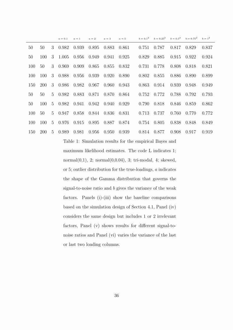
In the second scenario, we modify the fraction of the variance that is captured by the

common component relative to the total variance. In Section 4.1 we follow Doz, Giannone

& Reichlin (2012) and control the signal-to-noise ratio using di = βi/(1− βi), see equation

(16), with βi ∼ U(0.1, 0.9). This specification can be approximated by having a gamma

distribution with shape parameter a = 2 and scale parameter 1 for di. We consider this

approximation and vary the shape parameter for a = 0.1, 1, 2, 3, 5. This corresponds to

varying Var(λ′iαt)/Var(yi,t) by 0.9, 0.7, 0.5, 0.2, 0.1, respectively. We evaluate the influence

of the signal-to-noise ratio for the case where the loadings are drawn from the standard

normal distribution. Other sampling schemes for the loadings show the same results.

The results for the common components MSE comparison for different N, T combina-

tions are presented in Panel (v) of Table 1. We find that the relative gain of the empirical

Bayes estimates increases when the signal-to-noise ratio becomes lower, that is when a

increases. When the common component captures on average 90% of the variance, the

empirical Bayes estimates only provide modest relative gains. For N = 50 and T = 100,

there is even a small loss for the empirical Bayes estimates. When the signal-to-noise ratio

becomes smaller, the relative gain of the empirical Bayes estimates increases.

In the third and last scenario we modify the variance of some of the loading columns.

This has the effect that different factors explain different portions of the total variance.

In particular, when the true number of factors is r = 3 we take the variance of the third

loading column as b = 0.12, 0.252, 0.52, 0.752, or 12. The loadings in the other columns are

drawn from the standard normal distribution and all other features of the simulation design

are as in Section 4.1. For r = 5 we modify the variances of the fourth and fifth columns

23

using the same values for b. The results for the common components MSE comparison for

different N, T combinations are presented in Panel (vi) of Table 1. Notice that for b = 12,

the results correspond to those in the first column of panel (iii).

For this experiment we also find that the empirical Bayes estimates outperform the

maximum likelihood estimates, even when the strength of selected factors decreases from

equally strong to weak. For example, the difference in relative accuracy of the common

components estimates can vary up to 10% for a model with r = 3, when the variance of one

factor changes from b = 0.12 to b = 1. It shows to some extent that the empirical Bayes

methods are more able to empirically identify weak factors. Based on these results from

panels (iv), (v) and (vi), we carefully conjecture that empirical Bayes methods can perform

well in applications where the factors are weak or when irrelevant factors are included.

4.4 Additional simulation results

We briefly discuss several findings that are presented in detail in the web-appendix. First,

we have compared the empirical Bayes and maximum likelihood estimates to the principal

components estimates. Comparisons were based on the common components and showed

that both the empirical Bayes and maximum likelihood estimates outperform the principal

components estimates. This was already documented for maximum likelihood estimation

by Doz, Giannone & Reichlin (2012) and Bai & Li (2012) using trace statistics. We confirm

their conclusions using rMSE statistics.

Second, we complement the results in Table 1 for observation disturbances with only

serial correlation, only cross-sectional correlation, or neither serial correlation and cross-

sectional correlation. These results are very similar to those presented in Panels (i), (ii)

and (iii) of Table 1. This should not be surprising since the empirical Bayes and the

maximum likelihood estimates are affected to the same extent by misspecification. Hence

the relative statistics should remain the same overall, when the signal-to-noise ratio is kept

constant.

24

5 Macroeconomic forecasting

Our empirical study is concerned with the comparison of the empirical Bayes and maximum

likelihood approaches for dynamic factor models based on a quarterly U.S. macroeconomic

dataset. The key question is whether and to what extent the empirical Bayes methods

improve out-of-sample forecasts when compared to the maximum likelihood methods. We

consider the data set of Stock & Watson (2012), which includes N = 144 macro economic

and financial time series. These series capture a large part of the available disaggregated

macroeconomic and financial time series. Table 2 summarizes the categories for which the

time series are included. There are 13 different blocks including large blocks for employment

series and prices. Each block is indexed by a letter. From this data set we construct

stationary quarterly time series following the guidelines in the web-appendix of Stock &

Watson (2012). The resulting panel ranges from 1959-1 until 2008-4, with T = 200. The

panel is unbalanced and the estimation methods of Section 3 are adjusted accordingly as

discussed in the web-appendix.

We consider the dynamic factor model (2) with stochastic loadings and with conditions

of Assumption 1. The loadings and factors are identified up to an orthonormal rotation

matrix which is sufficient for forecasting applications. We follow Stock & Watson (2012)

and Jungbacker & Koopman (2015) and consider dynamic factor models with r = 5 and

r = 7 factors. We first discuss the full sample parameter estimation results, then we discuss

the details of our forecasting exercise and, finally, we present the results.

INSERT TABLE 2 AROUND HERE

5.1 Estimation results

In Table 3 we present the parameter estimates that define the the distributions of the

loadings and the factors. The methods of Section 3 are used to obtain the estimates. Prior

25

to estimation we have demeaned each time series. In the top panel of Table 3 we present

the estimates of the autoregressive matrix H . From the eigenvalues it follows that all the

factors are estimated as stationary processes. The factors are persistent since the largest

eigenvalues for both r = 5 and r = 7 are above 0.9. Additionally, we find some evidence

for persistent cyclical behavior in the factors. For the five factor model one conjugate pair

of complex eigenvalues is obtained with its real part equal to 0.809. The remaining two

eigenvalues are relatively small. For the seven factor model we have two conjugate pairs

with real parts equal to 0.775 and 0.102. Since the vector autoregressive (VAR) process of

the factors impose a zero mean and an identity variance matrix, we can relate the individual

coefficients in H to each other. However, as for any VAR analysis, individual coefficients

in H do not have a clear interpretation.

In the bottom panel of Table 3 we report the estimates for the means and variances

of the loading matrices. The mean coefficients are small and typically close to zero. The

diagonal elements of the variance matrices indicate that the variance in the loadings is

small. However, the variances of the different loading columns are not equivalent indicating

that some of the factors are stronger relative to others.

In Figure 1 we show the empirical density function and histograms of the estimates for

the columns of the loading matrix. The third and fourth loading columns show multiple

modes, whereas the first is slightly skewed to the left. All empirical distributions are

quite similar to the normal distribution, with standard deviations between 0.1 and 0.2

approximately. However, the tails of the distributions are often heavier when compared to

the normal distribution. In the lower right of Figure 1 we show the empirical distribution

for all loadings. This distribution is skewed to the right.

In the web-appendix we show the estimated factors and the correlations of the factors

with the individual time series. Since the model is identified subject to rotation, the em-

pirical Bayes and maximum likelihood methods typically identify a different rotation. This

implies that only the inner-products are comparable. For a selection of time series we show

26

the estimated inner-products. We find that the estimates are close but not identical.

INSERT TABLE 3 AROUND HERE

INSERT FIGURE 1 AROUND HERE

5.2 Forecasting study

The out-of-sample forecasting study for the panel of macroeconomic time series is designed

as follows. For the models with r = 5 and r = 7 factors we forecast each time series

1, 2 and 4 quarters ahead for 1985-1 until 2008-4. In total we compute m = 96 out-of

sample predictions for each horizon and model. In particular, let the integer n denote

the sample split point (1984-4 for h = 1, 1984-3 for h = 2 and 1984-1 for h = 4). The

forecasts are computed for n+ 1, . . . , n+m based on sequentially demeaned subsamples of

the observations y1, . . . ,yn+j−h, for j = 1, . . . ,m. We estimate the parameter vector ψ for

each subsample using the methods of Section 3.

Based on the estimated parameter vectors we compute the empirical Bayes posterior

mode and maximum likelihood forecasts by

yn+j = Λαn+j and yn+j = Λαn+j,

where αn+j = E(αn+j|y1, . . . ,yn+j−h; Λ; ψ) is the posterior mode forecast for the factors

and αn+j = E(αn+j|y1, . . . ,yn+j−h; Λ; ψ1) is the forecast for the factors based on the max-

imum likelihood estimates. These forecasts are computed for horizons h = 1, 2, 4. We add

the sample mean of the subsample to the forecasts before determining its accuracy.

As a measure of accuracy we consider the mean squared error (MSE) of the out-of-sample

27

forecasts. In particular we compute for each time series

MSEPEBi = m−1

m∑j=1

(yi,n+j − yi,n+j)2 and MSEMLEi = m−1

m∑j=1

(yi,n+j − yi,n+j)2, (18)

where yi,n+j and yi,n+j are the ith elements of yn+j and yn+j, respectively. In this way we

compute mean squared error statistics for 144 time series for all forecasting horizons.

5.3 Forecasting results

In Table 4 we present summary statistics for the relative mean squared error statistics, that

is MSEPEBi /MSEMLE

i for i = 1, . . . , 144. For the model with r = 5 factors the one quarter

ahead forecasts of the empirical Bayes estimates are on average 8% more accurate, this

decreases to 3% for the two quarters ahead forecasts and to 1% for the four quarters ahead

forecasts. For the model with r = 7 factors the relative gains are larger. In particular,

for one quarter ahead the gain is 12% which decreases to 5% and 2% for the two and

four quarter ahead forecasts, respectively. We have obtained some substantial forecasting

gains for shorter forecast horizons. The relative improvement in accuracy of empirical

Bayes forecasts declines as we forecast further into the future. This is not surprising since

both the empirical Bayes and maximum likelihood estimates are based on the same vector

autoregressive process for the factors. The out-of sample forecasting variance for a larger

forecast horizon is dominated by the contribution of the factors given that the loadings are

time-invariant.

We further present a selection of quantiles of the distributions. For the 0.05 quantile,

we find gains between 30% and 15% depending on the forecast horizon. This indicates

that for a modest number of time series the gains are very large. On the other side of the

distribution, the relative accuracy is somewhat more in favor of the maximum likelihood

estimates. Here we can even lose 18% for some time series.

Finally, we summarize the relative mean squared error statistics per category. We find

28

that the largest gains are obtained for the real economic categories such as Housing (this

includes series related to housing starts), Inventories and Employment. For the category of

Wages, Prices and Money we do not obtain improvements for the empirical Bayes methods.

The largest gains are found for the time series that load strongly on the factors.

INSERT TABLE 4 AROUND HERE

6 Conclusion

We have developed parametric empirical Bayes methods for the estimation of the dynamic

factor model. The loadings, factors and disturbances of the model are treated as latent

stochastic variables, which follow Gaussian distributions. For the estimation of the load-

ings and factors we have developed a posterior mode algorithm which relies on standard

methods for linear time series and regression models. The parameter vector is estimated

by likelihood-based methods using a simple two-step implementation. The posterior means

and variances of the loadings are estimated by standard simulations methods. We circum-

vent the infinite variance problem by calculating the integral over the factors analytically.

We emphasize that the computational effort for the empirical Bayes methods is only mod-

estly larger when compared to standard maximum likelihood methods; see Doz, Giannone

& Reichlin (2012) and Jungbacker & Koopman (2015).

The methods are evaluated in a Monte Carlo study for dynamic factor models with

different dimensions and different numbers of factors. For the common components the

empirical Bayes estimates always outperform the maximum likelihood estimates for the

data generating processes considered. The relative gains increase when the data generating

process includes irrelevant or weak factors. We have further illustrated our methods in

an empirical application for forecasting macroeconomic time series. The empirical Bayes

approach again dominates the maximum likelihood approach.

29

References

Aguilar, Omar & Mike West. 2000. “Bayesian Dynamic Factor Models and Portfolio

Allocation.” Journal of Business and Economic Statistics 18:338–357.

Anderson, Brian D. O. & John B. Moore. 1979. Optimal Filtering. Englewood Cliffs:

Prentice-Hall.

Bai, Jushan & Kunpeng Li. 2012. “Statistical Analysis of Factor Models of High

Dimension.” The Annals of Statistics 40:436–465.

Bai, Jushan & Kunpeng Li. 2015. “Maximum Likelihood Estimation and Inference for

Approximate Factor Models of High Dimension.” Review of Economics and Statistics

. forthcoming.

Bai, Jushan & Serena Ng. 2002. “Determining the Number of Factors in Approximate

Factor Models.” Econometrica 70:191–221.

Bai, Jushan & Serena Ng. 2008. “Large Dimensional Factor Analysis.” Foundations and

Trends in Econometrics 3:89–163.

Banbura, Martha & Michele Modugno. 2014. “Maximum Likelihood Estimation of Factor

Models on Datasets with Arbitrary Pattern of Missing Data.” Journal of Applied

Econometrics 29:133–160.

Bernanke, Ben S., Jean Boivin & Piotr Eliasz. 2005. “Measuring the Effects of Monetary

Policy: A Factor-Augmented Vector Autoregressive (FAVAR) Approach.” Quarterly

Journal of Economics 120:387–422.

Besag, Julian. E. 1986. “On the Statistical Analysis of Dirty Pictures.” Journal of the

Royal Statistical Society, Series B 48:259–302.

30

Bhattacharya, Anirban & David B. Dunson. 2011. “Sparse Bayesian infinite factor

models.” Biometrika 98:291–306.

Bishop, Christopher M. 2006. Pattern Recognition and Machine Learning. New York:

Springer.

Chan, J. & I. Jeliazkov. 2009. “Efficient Simulation and Integrated Likelihood Estimation

in State Space Models.” International Journal of Mathematical Modelling and

Numerical Optimisation 1:101–120.

Chan, J., R. Leon-Gonzalez & R. W. Strachan. 2013. “Invariant Inference and Efficient

Computation in the Static Factor Model.”. Working Paper.

Doornik, Jurgen A. 2007. Object-Oriented Matrix Programming Using Ox. London:

Timberlake Consultants Press.

Doucet, Arnaud N., Nando de Freitas & Neil J. Gordon. 2001. Sequential Monte Carlo

Methods in Practice. New York: Springer Verlag.

Doz, Catherine, Domenico Giannone & Lucrezia Reichlin. 2012. “A Quasi Maximum

Likelihood Approach for Large Approximate Dynamic Factor Models.” Review of

Economics and Statistics 94:1014–1024.

Durbin, James & Siem Jan Koopman. 2012. Time Series Analysis by State Space

Methods. Oxford: Oxford University Press.

Efron, Brad. 2010. Large Scale Inference, Empirical Bayes Methods for Estimation,

Testing, and Prediction. Cambridge: Cambridge University Press.

Efron, Brad & Carl Morris. 1973. “Stein’s Estimation Rule and Its Competitors.” Journal

of the American Statistical Association 68:117–130.

31

Geweke, John F. 1989. “Bayesian Inference in Econometric Models Using Monte Carlo

Integration.” Econometrica 57:1317–1339.

James, Willard & Charles Stein. 1961. Estimation with Quadratic Loss. In Proceedings of

the Third Berkeley Symposium on Mathematical Statistics and Probability, ed. J.

Neyman. Berkeley: University of California Press pp. 361–379.

Julier, Simon J. & Jeffrey K. Uhlmann. 1997. A new extension of the Kalman filter to

nonlinear systems. In Signal Processing, Sensor Fusion, and Target Recognition VI,

ed. I. Kadar. Vol. 3068 SPIE pp. 182–193.

Jungbacker, Boris & Siem Jan Koopman. 2007. “Monte Carlo Estimation for Nonlinear

Non-Gaussian State Space Models.” Biometrika 94:827–839.

Jungbacker, Boris & Siem Jan Koopman. 2015. “Likelihood-based Analysis for Dynamic

Factor Analysis for Measurement and Forecasting.” Econometrics Journal

18:C1–C21.

Kaufmann, Sylvia & Christian Schumacher. 2013. “Bayesian estimation of sparse dynamic

factor model with order-independent identification.”. Working paper.

Kim, H. H. & N. R. Swanson. 2014. “Forecasting financial and macroeconomic variables

using data reduction methods: New empirical evidence.” Journal of Econometrics

178:352–367.

Knox, Thomas, James H. Stock & Mark W. Watson. 2004. “Empirical Bayes Regression

With Many Regressors.”. Working paper.

Koopman, Siem Jan, Andre Lucas & Marcel Scharth. 2014. “Numerically Accelerated

Importance Sampling for Nonlinear Non-Gaussian State Space Models.” Journal of

Business and Economic Statistics 32:forthcoming.

32

Koopman, Siem Jan & Neil Shephard. 1992. “Exact score for time series models in state

space form.” Biometrika 79:823–826.

Marron, J. Steve & Matt P. Wand. 1992. “Exact Mean Integrated Squared Error.” The

Annals of Statistics 20:712–736.

McCausland, W. J., S. Miller & D. Pelletier. 2011. “Simulation smoothing for state-space

models: a computational efficiency analysis.” Computational Statistics and Data

Analysis 55:199–212.

Meng, Xiao-Li & Donald B. Rubin. 1993. “Maximum Likelihood Estimation via the ECM

Algorithm: A General Framework.” Biometrika 80:267–278.

Mesters, Geert & Siem Jan Koopman. 2014. “Generalized Dynamic Panel Data Models

with Random Effects for Cross-Section and Time.” Journal of Econometrics

154:127–140.

Nakajima, Jouchi & Mike West. 2013. “Bayesian Analysis of Latent Threshold Dynamic

Models.” Journal of Business and Economic Statistics 31:151–164.

Newey, Whitney K. & Daniel L. McFadden. 1994. Large sample estimation and

hypothesis testing. In Handbook of Econometrics, ed. R. F. Engle & D. L. McFadden.

Amsterdam: Elsevier pp. 2111–2245.

Onatski, A. 2009. “Testing Hypotheses About the Number of Factors in Large Factor

Models.” Econometrica 77:1447–1479.

Onatski, A. 2012. “Asymptotics of the principal components estimator of large factor

models with weakly influential factors.” Journal of Econometrics 168:244–258.

Onatski, A. 2015. “Asymptotic Analysis of the Squared Estimation Error in Misspecified

Factor Models.” Journal of Econometrics 186:388–406.

33

So, Mike K. P. 2003. “Posterior mode estimation for nonlinear and non-Gaussian state

space models.” Statistica Sinica 13:255–274.

Stock, James H. & Mark W. Watson. 2002a. “Forecasting Using Principal Components

From a Large Number of Predictors.” Journal of the American Statistical Association

97:1167–1179.

Stock, James H. & Mark W. Watson. 2002b. “Macroeconomic Forecasting Using Diffusion

Indexes.” Journal of Business and Economic Statistics 220:147–162.

Stock, James H. & Mark W. Watson. 2005. “Implications of Dynamic Factor Models for

VAR Analysis.”. manuscript.

Stock, James H. & Mark W. Watson. 2011. Dynamic Factor Models. In Oxford Handbook

of Economic Forecasting, ed. M. P. Clements & D. F. Hendry. Oxford: Oxford

University Press.

Stock, James H. & Mark W. Watson. 2012. “Generalized Shrinkage Methods for

Forecasting Using Many Predictors.” Journal of Business and Economic Statistics

30:481–493.

34

Panel (i): rMSE(λ) Panel (ii): rMSE(α)

N T r L=1 L=2 L=3 L=4 L=5 L=1 L=2 L=3 L=4 L=5

50 50 3 0.885 0.911 0.896 0.863 0.886 0.975 0.976 0.986 0.979 0.963

50 100 3 1.123 1.094 1.125 1.073 1.119 0.981 0.979 0.967 0.953 0.980

100 50 3 0.836 0.858 0.840 0.783 0.843 1.295 1.293 1.327 1.233 1.269

100 100 3 0.929 0.939 0.934 0.882 0.929 0.987 0.985 0.998 0.983 0.976

150 200 3 1.038 1.033 1.042 1.008 1.041 0.999 0.993 0.995 0.981 1.000

50 50 5 0.866 0.902 0.872 0.871 0.860 0.979 0.979 0.986 0.989 0.974

50 100 5 1.082 1.063 1.076 1.047 1.049 0.915 0.912 0.912 0.903 0.908

100 50 5 0.772 0.804 0.777 0.745 0.764 1.229 1.227 1.253 1.204 1.214

100 100 5 0.897 0.911 0.902 0.865 0.889 0.984 0.983 0.989 0.984 0.976

150 200 5 1.002 1.002 1.006 0.962 1.002 0.956 0.955 0.954 0.948 0.958

Panel (iii): rMSE(λ′α) Panel (iv): rMSE(λ′α)

L=1 L=2 L=3 L=4 L=5 L=1 L=2 L=3 L=4 L=5

50 50 3 0.837 0.884 0.855 0.778 0.841 0.720 0.786 0.761 0.727 0.686

50 100 3 0.924 0.955 0.914 0.856 0.941 0.777 0.820 0.808 0.786 0.734

100 50 3 0.821 0.909 0.839 0.754 0.819 0.689 0.792 0.730 0.687 0.655

100 100 3 0.899 0.917 0.903 0.837 0.899 0.714 0.756 0.753 0.730 0.668

150 200 3 0.949 0.958 0.949 0.909 0.962 0.724 0.743 0.760 0.732 0.666

50 50 5 0.793 0.857 0.800 0.758 0.784 0.723 0.807 0.748 0.737 0.695

50 100 5 0.862 0.894 0.869 0.815 0.848 0.770 0.800 0.800 0.798 0.733

100 50 5 0.773 0.856 0.786 0.713 0.758 0.673 0.772 0.698 0.679 0.634

100 100 5 0.849 0.876 0.855 0.780 0.839 0.684 0.734 0.716 0.703 0.643

150 200 5 0.919 0.927 0.919 0.866 0.926 0.684 0.706 0.710 0.699 0.642

Panel (v): rMSE(λ′α) Panel (vi): rMSE(λ′α)

35

a = 0.1 a = 1 a = 2 a = 3 a = 5 b = 0.12 b = 0.252 b = 0.52 b = 0.752 b = 12

50 50 3 0.982 0.939 0.895 0.883 0.861 0.751 0.787 0.817 0.829 0.837

50 100 3 1.005 0.956 0.949 0.941 0.925 0.829 0.885 0.915 0.922 0.924

100 50 3 0.969 0.909 0.865 0.855 0.832 0.731 0.778 0.808 0.818 0.821

100 100 3 0.988 0.956 0.939 0.920 0.890 0.802 0.855 0.886 0.890 0.899

150 200 3 0.986 0.982 0.967 0.960 0.943 0.863 0.914 0.939 0.948 0.949

50 50 5 0.982 0.883 0.871 0.870 0.864 0.752 0.772 0.788 0.792 0.793

50 100 5 0.982 0.941 0.942 0.940 0.929 0.790 0.818 0.846 0.859 0.862

100 50 5 0.947 0.858 0.844 0.836 0.831 0.713 0.737 0.760 0.770 0.772

100 100 5 0.976 0.915 0.895 0.887 0.874 0.754 0.805 0.838 0.848 0.849

150 200 5 0.989 0.981 0.956 0.950 0.939 0.814 0.877 0.908 0.917 0.919

Table 1: Simulation results for the empirical Bayes and

maximum likelihood estimates. The code L indicates 1;

normal(0,1), 2; normal(0,0.04), 3; tri-modal, 4; skewed,

or 5; outlier distribution for the true-loadings, a indicates

the shape of the Gamma distribution that governs the

signal-to-noise ratio and b gives the variance of the weak

factors. Panels (i)-(iii) show the baseline comparisons

based on the simulation design of Section 4.1, Panel (iv)

considers the same design but includes 1 or 2 irrelevant

factors, Panel (v) shows results for different signal-to-

noise ratios and Panel (vi) varies the variance of the last

or last two loading columns.

36

Category number of series (144)

A GDP components 16

B Industrial production 14

C Employment 20

D Unemployment rate 7

E Housing starts 6

F Inventories 6

G Prices 37

H Wages 6

I Interest rates 13

J Money 8

K Exchange rates 5

L Stock prices 5

M Consumer expectations 1

Table 2: Summary of the time series that are included in

the empirical application

37

Eigenvalues

Autoregressive coefficients H real img

5 factors

0.911 0.065 -0.161 -0.287 -0.094 0.945 0.000

0.049 0.656 0.364 0.103 -0.183 0.811 0.110

0.014 0.278 0.555 0.090 0.048 0.811 -0.110

0.064 -0.331 -0.056 0.454 -0.532 0.445 0.000

0.016 0.009 -0.059 -0.103 0.700 0.264 0.000

7 factors

0.628 0.280 0.036 -0.174 0.199 0.084 -0.103 0.935 0.000

0.173 0.624 -0.207 -0.211 -0.023 0.287 0.062 0.775 0.116

0.201 -0.123 0.671 0.203 -0.284 0.041 0.016 0.775 -0.116

-0.095 -0.010 0.073 0.261 0.074 0.012 -0.062 0.774 0.000

0.120 -0.252 -0.195 -0.046 0.585 -0.389 -0.358 0.255 0.000

-0.138 0.043 0.085 -0.023 0.008 0.353 -0.280 0.102 0.120

-0.287 0.182 -0.164 -0.046 0.035 -0.229 0.597 0.102 0.120

Distribution loadings Σλ δ

5 factors

0.034 -0.054 -0.025 -0.015 -0.072 -0.038

-0.054 0.231 -0.015 -0.036 0.202 0.105

-0.025 -0.015 0.065 0.080 0.043 0.028

-0.015 -0.037 0.080 0.145 0.040 0.023

-0.072 0.202 0.043 0.040 0.235 0.125

38

7 factors

0.055 0.018 0.011 0.047 -0.060 -0.001 0.087 0.027

0.018 0.070 0.006 0.000 -0.016 0.098 0.107 0.065

0.011 0.006 0.047 0.034 -0.026 -0.030 0.061 0.010

0.047 0.000 0.034 0.073 -0.061 -0.045 0.092 0.012

-0.060 -0.016 -0.026 -0.061 0.077 0.020 -0.105 -0.030

-0.001 0.098 -0.030 -0.045 0.020 0.186 0.097 0.088

0.087 0.107 0.061 0.092 -0.105 0.097 0.306 0.124

Table 3: Parameter estimates for the vector autoregres-

sive coefficients and the mean and variance of the load-

ings for the factor models with r = 5 and r = 7 factors.

The full sample of observations is used (N = 144 and

T = 200) and we estimate the model parameters using

the methods developed in Section 3. The columns indi-

cated by Eigen summarize the real and imaginary eigen-

values of the matrix H in decreasing order.

39

Loading #1

-0.4 -0.2 0.0 0.2 0.4

2

4

6Loading #1 Loading #2

-0.75 -0.50 -0.25 0.00 0.25 0.50

1

2

3

4Loading #2

Loading #3

-0.50 -0.25 0.00 0.25 0.50 0.75

1

2Loading #3 Loading #4

-0.2 0.0 0.2 0.4

2

4Loading #4

Loading #5

-0.5 0.0 0.5 1.0

1

2

3Loading #5 All Loadings

-0.5 0.0 0.5 1.0

1

2

3 All Loadings

Figure 1: Empirical density function (solid line) and histograms for the posterior modes ofthe columns of the loading matrix. We present the results per column and for all columnscombined.

r = 5 Factors r = 7 Factors

h = 1 h = 2 h = 4 h = 1 h = 2 h = 4

All series

Mean 0.912 0.979 0.994 0.874 0.951 0.978

Quantiles

0.05 0.762 0.828 0.861 0.696 0.766 0.819

0.25 0.893 0.930 0.940 0.847 0.915 0.931

0.50 0.979 0.984 0.992 0.932 0.993 0.993

0.75 1.028 1.025 1.024 1.023 1.026 1.033

0.95 1.176 1.123 1.142 1.129 1.102 1.187

40

Components (Mean)

GDP components 0.901 0.925 0.932 0.832 0.966 0.950

Industrial Production 0.958 0.973 0.981 0.838 0.894 0.911

Employment 0.829 0.829 0.876 0.838 0.857 0.866

Unemployment rate 0.988 0.969 0.975 1.031 0.994 0.989

Housing 0.853 0.943 0.992 0.727 0.844 0.940

Inventories 0.701 0.869 0.906 0.661 0.868 0.901

Prices 1.063 1.069 1.065 1.041 1.021 1.054

Wages 1.010 0.992 0.989 0.961 0.958 0.982

Interest rates 0.973 1.004 1.006 0.915 0.937 0.957

Money 1.302 0.997 1.001 1.458 1.004 1.006

Exchanges rates 1.032 1.011 1.011 1.053 1.034 1.022

Stock prices 1.046 0.973 1.011 1.096 0.985 1.023

Consumer Expectations 0.930 0.976 0.999 0.921 0.981 0.996

Table 4: Relative mean squared error statistics for out-of-

sample forecasting using the empirical Bayes method and

the maximum likelihood method. The results summarize

the distribution of the statistics MSEPEBi /MSEMLE

i , for

i = 1, . . . , 144 and forecast horizons h = 1, 2, 4.

41