Advances in Pure Mathematics, 2019, 9, 619-628 http://www.scirp.org/journal/apm

ISSN Online: 2160-0384 ISSN Print: 2160-0368

DOI: 10.4236/apm.2019.97031 Jul. 31, 2019 619 Advances in Pure Mathematics

Empirical Analysis of Gross Domestic Product and Coal Import Based on VAR Model

Shichang Shen, Chao Feng

School of Mathematics and Statistics, Qinghai Nationalities University, Xining, China

Abstract The speed of China’s economic development is gradually accelerating, and the demand for energy is also constantly increasing, especially the demand for coal. In order to reveal whether the coal imports have an impact on China’s economic development, this paper constructs the VAR(6) model by selecting the quarterly data of coal imports (CIV) and gross domestic product (GDP) from 2002 to 2017, performing ADF (Augmented Dickey-Fuller) stationarity test and Johansen cointegration test. It shows that there is a long-term stable equilibrium relationship between coal imports and GDP. Then the impulse response function is used to obtain the relationship between coal imports and GDP. It is found that the impact of coal imports on GDP is greater than the impact of GDP on coal imports.

Keywords Coal Imports, Gross Domestic Product, VAR Model, Impulse Response Function

1. Introduction

China’s economy has developed rapidly, and the total amount of GDP has in-creased year by year. China has become the largest developing country. At the same time of economic development, the problem of energy consumption has become increasingly prominent, especially the amount of coal used. China is a big country in coal use, especially using coal for power generation. Therefore, most of the coal used in China at this stage is imported, so it is particularly im-portant to explore the relationship between coal imports and GDP. Chang Jun-feng [1] used the relevant regression analysis method to predict and discuss GDP and coal consumption (price).

Ma Yuanxin [2] dynamically described the long-term equilibrium relationship

How to cite this paper: Shen, S.C. and Feng, C. (2019) Empirical Analysis of Gross Domestic Product and Coal Import Based on VAR Model. Advances in Pure Mathe-matics, 9, 619-628. https://doi.org/10.4236/apm.2019.97031 Received: July 3, 2019

Accepted: July 28, 2019 Published: July 31, 2019 Copyright © 2019 by author(s) and Scientific Research Publishing Inc. This work is licensed under the Creative Commons Attribution International License (CC BY 4.0). http://creativecommons.org/licenses/by/4.0/

Open Access

S. C. Shen, C. Feng

DOI: 10.4236/apm.2019.97031 620 Advances in Pure Mathematics

between coal consumption and economic growth in Shanxi Province through cointegration analysis and Granger causality test. Wu Yongping [3] also described the relationship between coal consumption and economic growth in the world’s major coal-consuming countries through cointegration analysis and Granger cau-sality test. Chen Weidong [4] mainly adopts quantitative analysis to establish a VAR model of coal price and GDP, and dynamically analyzes the long-term im-pact of coal price on economic growth. Zhou Aiqian [5] analyzed the long-term impact of China’s coal price on economic growth. Xie Changfeng [6] used the panel data model and VAR model to analyze the energy consumption and eco-nomic growth in Jiangsu, Zhejiang and Shanghai. In the past, scholars mainly analyzed the relationship between coal prices and economic growth. This paper establishes a VAR model for coal imports and economic growth(GDP), and de-termines the long-term stable equilibrium relationship between the two through Johansen cointegration test. The impulse response function is used to further ex-plain the dynamics relationship between coal imports and GDP.

2. Theoretical Basis 2.1. VAR Model

The VAR model, also known as the vector auto-regressive model, is commonly used to predict multivariate time series systems and to describe the dynamic ef-fects of random perturbation terms on variable systems. The general form of the VAR(p) model is as follows:

1 1 1t t p t p t r t r ty A y A y B x B x ε− − −= + + + + + + (1)

where, ty is a m-dimensional endogenous variable vector, tx is a d-dimensional endogenous variable vector. 1, , pA A and 1, , rB B are the parameter ma-trices to be estimated, p is the lag period of the endogenous variable, r is the lag period of the exogenous variable. tε is a random disturbance term, which can be related to the same period, but not autocorrelation.

2.2. Johansen Cointegration Test

The Johansen cointegration test includes a trace test and a maximum eigen value test.

The assumption of the trace test is: H0: at most r cointergration relations H1: m cointergration relations (full rank) The test statistic is:

( ) ( )1

| ln 1m

tr ii r

LR r m T λ= +

= − −∑ (2)

where iλ is the eigenvalue of row i of the size row, T is the total number of ob-servation periods.

The assumption of the maximum eigenvalue test is: H0r: there are r cointegration relations H1r: at least r + 1 cointegration relations The test statistic is:

S. C. Shen, C. Feng

DOI: 10.4236/apm.2019.97031 621 Advances in Pure Mathematics

( ) ( )( ) ( )

max 1| 1 ln 1

| 1 | , 0,1, , 1r

tr

LR r r T

LR r m LR r m r m

λ ++ = − −

= − + = −

(3)

2.3. Impulse Response Function

According to the VAM(p) form of the VAR(∞) model, the generalized impulse response function of the VAR model is represented by a matrix as:

( ) 1 2 , 0qj jj q j qσ −Ψ = Θ Σ = (4)

2.4. LR Test Statistic

Likelihood ratio test is divided into two models: unconstrained and constrained. The likelihood ratio statistic refers to the difference between the maximum like-lihood of the unconstrained model and the constraint model, that is:

( ) ( )22 ~u rLR l l kχ= − (5)

where ul and represent the maximum likelihood estimates of the uncon-strained model and the constrained model for an observed sample condition. k is a positive integer, indicating the degree of freedom of the chi-square distribution, equal to the number of constrains.

2.5. Final Prediction Error

The final prediction error takes the minimum value of p in the formula as the best order of the VAR model.

( ) ( )( )

2ˆFPE p

n kp

n kσ

+=

− (6)

where 2ˆ pσ is the variance estimate of the residual at the time of the lag p period, n is the sample size, and k is the number of parameters to be estimated.

2.6. Information Guidelines

In order to find a balance between the lag period and the degree of freedom, the order is generally determined according to the criteria for the minimum value of AIC (Akaike info criterion), SC (Schwarz criterion) and HQ (Hannan-Quinn criterion) information. The formula is as follows:

AIC 2 2l n k n= − + (7)

SC 2 lnl n k n n= − + (8)

( )HQ 2 2 ln lnl n k n n= − + (9)

where ( )k m rd pm= + is the number estimated parameters, n is the number of observations.

3. Empirical Analysis 3.1. Data Selection and Processing

This paper selects the most representative economic indicator GDP (gross do-

S. C. Shen, C. Feng

DOI: 10.4236/apm.2019.97031 622 Advances in Pure Mathematics

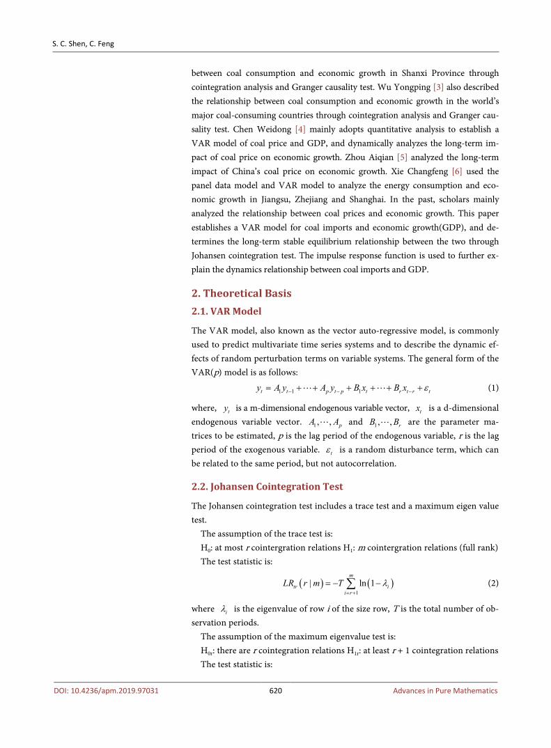
mestic product) to represent the status quo of economic development, and uses the index of coal imports to measures the dynamic relationship with GDP. Therefore, this paper takes the GDP and coal import data from the first quarter of 2002 to the fourth quarter of 2017 as the sample time series, and records them as GDP and CIV. Figure 1 shows the trend of GDP and CIV. The data comes from the China Statistical Yearbook and the Energy Comprehensive Database. In order to avoid the influence of the heteroscedasticity of the time series data on the empirical analysis, the original sequence is logarithmized, and the new se-quence is recorded as LnGDP and LnCIV.

This paper uses Eviews 7.2 [7] [8] to perform corresponding data analysis. It can be seen from Figure 1 that the sequence GDP and CIV have obvious

trends and are not stable.

3.2. Stationarity Test

The establishment of VAR model theoretically requires time series data to be stable. In this paper, the ADF (Augmented Dickey-Fuller) unit root test is used to test the stationarity of the original sequence and the logarithmized new se-quence. The lag order P is selected by SC criterion. The test results are shown in Table 1. From the results of Table 1, it can be seen that the sequence GDP, CIV and the logarithmized new sequence LnGDP and LnCIV did not pass the statio-narity test.

In order to make the sequence stable, the logarithmized sequence is first-order differential, and the differenced sequence is recorded as DLnGDP, DLnCIV, and then the ADF unit root test is performed on the two sequences. The test results are shown in Table 2.

Table 1. ADF test of GDP, CIV, LnGDP and LnCIV sequences.

Variable Inspection

type ADF test

value 1% level

threshold 5% level

threshold 10% level threshold

Conclusion

GDP (0, 0, 5) 2.71515 −2.61606 −1.94665 −1.61312 Unstable

CIV (0, 0, 3) −0.00299 −2.60279 −1.94616 −1.61340 Unstable

LnGDP (0, 0, 5) 2.38193 −2.60616 −1.94665 −1.61312 Unstable

LnCIV (0, 0, 3) 1.21909 −2.60279 −1.94616 −1.61340 Unstable

Note: The three items in the test type represent the constant term, the time trend term, and the lag order in the stationarity test, respectively. Table 2. ADF test of DLnGDP and DLnCIV sequences.

Variable Inspection

type ADF test

value 1% level

threshold 5% level

threshold 10% level threshold

Conclusion

DLnGDP (0, 0, 2) −7.75932 −2.60475 −1.94645 −1.61324 Smooth

DLnCIV (0, 0, 3) −8.27376 −2.60342 −1.94625 −1.61335 Smooth

S. C. Shen, C. Feng

DOI: 10.4236/apm.2019.97031 623 Advances in Pure Mathematics

Figure 1. Time series diagram of GDP and CIV.

It can be seen from the results of Table 2 that the sequence after the

first-order difference is stable, and both the DLnGDP and the DLnCIV se-quences are first-order single-order sequences.

3.3. Recognition of VAR Model

The determination of the lag order is a very important issue when building a VAR model. In general, it is desirable that the lag order is large enough to effec-tively and completely reflect the dynamic characteristics of the model. However, the larger the lag order becomes, the more the estimated parameters in the mod-el will be. At the same time, it can reduce the freedom of the model. Therefore, we should consider the problem of lag order and degree of freedom at the same time, and find a state of equilibrium. Commonly used methods are LR (likelih-ood ratio) test, final prediction error (FPE), AIC information criterion, SC in-formation criterion, HQ information criterion, and the optimal lag order is de-termined by the above method, as shown in Table 3.

It can be seen from the results in Table 3 that among the LR, FPE, AIC, SC and HQ values of the lag order from 0 to 7 orders, there are four criteria that se-lect the lag 6th order, so the order of the model is determined to be 6, and the VAR is established. The estimated results of the model are as follows:

S. C. Shen, C. Feng

DOI: 10.4236/apm.2019.97031 624 Advances in Pure Mathematics

Table 3. Judgment of lag order of VAR model.

Log LogL LR FPE AIC SC HQ

0 51.98333 NA 0.00056 −1.81758 −1.74459 −1.78935

1 60.69260 16.46843 0.00047 −1.98882 −1.76984 −1.90414

2 64.23896 6.447931 0.00048 −1.97233 −1.60736 −1.83119

3 106.1393 73.13513 0.00012 −3.35052 −2.83956 −3.15293

4 162.5236 94.31558 1.80e-05 −5.25540 −4.59846 −5.00136

5 178.9730 26.31909 1.15e-05 −5.70811 −4.90518* −5.39761

6 185.5256 10.00749* 1.06e-05* −5.80093* −4.85201 −5.43397*

7 187.2930 2.570825 1.16e-05 −5.71975 −4.62484 −5.29634

Note: “*” indicates the optimal order of choice.

1

1

2

2

3

DLnGDP DLnGDP0.518934 0.016185DLnCIV DLnCIV3.468739 0.052525

DLnGDP0.278057 0.010328DLnCIV1.305472 0.016166

DLnGDP0.146547 0.015008D0.087103 0.122838

t t

t t

t

t

t

−

−

−

−

−

= −

− + −

− + − 3

4

4

5

5

6

6

LnCIV

DLnGDP0.818583 0.001951DLnCIV0.251994 0.006464

DLnGDP0.662573 0.010260DLnCIV3.167198 0.017452

DLnGDP0.148278 0.021889DLnCIV1.283247 0.050427

t

t

t

t

t

t

t

−

−

−

−

−

−

−

− + −

+ −

+

0.0143160.044476

+

(10)

3.4. Stability Test of VAR Model

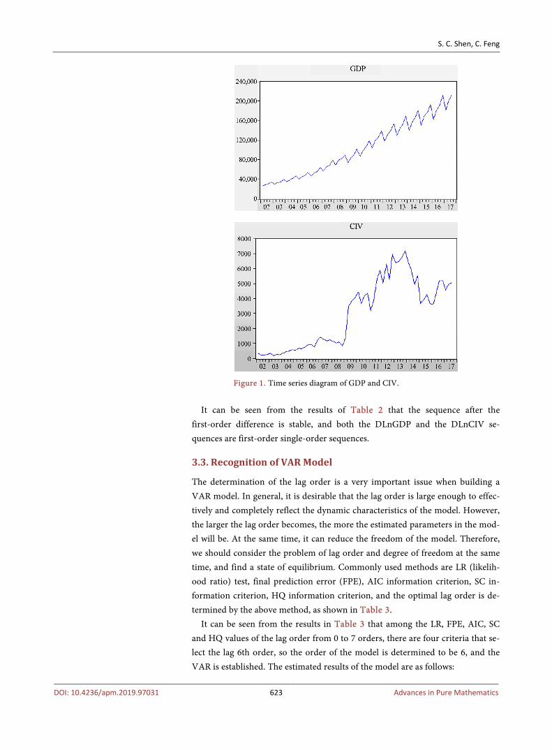
After estimating the parameters of the VAR model, it is necessary to perform an adaptive test on the model to ensure that the model meets the expected results. The most commonly used method is the reciprocal test of the root of the AR (auto-regressive) characteristic polynomial. The results are shown in Figure 2 and Table 4.

It can be seen from the results of Figure 2 and Table 4 that the reciprocal of all characteristic polynomial roots is less than 1, and within the unit circle, it in-dicates that the VAR(6) model is stable. The X and Y axes of Figure 2 represent the coefficients of the eigenvalues, respectively.

3.5. Johansen Cointegration Test

Since the logarithmic sequence LnGDP and LnCIV are not stable, the VAR model cannot be directly established. However, in the stationarity test of 3.1, the two sequences are known to be first-order single-sequences, so it can be tested by Johansen cointegration. To determine if there is a long-term stable equili-

S. C. Shen, C. Feng

DOI: 10.4236/apm.2019.97031 625 Advances in Pure Mathematics

brium relationship between variables, it is assumed that there is cointegration relationship between variables, indicating that the established VAR(6) model is reasonable. The lag of the cointegration test is 5, and the lag order of the VAR model is 6. The Johansen cointegration test is performed on the sequences LnGDP and LnCIV, and the results are shown in Table 5 and Table 6.

It can be seen from the results of Table 5 and Table 6 that Johansen cointe-gration rank test and maximum eigenvalue test show that there is a cointegra-tion relationship between variable GDP and CIV, and there is a cointegration vector with long-term stable equilibrium relationship. Therefore, the established VAR(6) model is reasonable.

Figure 2. VAR model adaptability test.

Table 4. AR root of VAR model.

Root Modulus

−0.997734 0.997734

−0.000536-0.994724i 0.994725

−0.000536+0.994724i 0.994725

0.890484 0.890484

0.775665-0.449389i 0.879192

0.755655+0.499389i 0.879192

0.318943-0.686363i 0.756848

0.318943+0.686363i 0.756848

−0.353061-0.635243i 0.726764

−0.353061+0.635243i 0.726764

−0.590099 0.590099

−0.169214 0.169214

S. C. Shen, C. Feng

DOI: 10.4236/apm.2019.97031 626 Advances in Pure Mathematics

Table 5. Johansen cointegration rank test results.

Hypothesized Eigenvalue Trace 0.05 Prob.**

None* 0.346778 26.64030 15.49471 0.0007

At most 1 0.048657 2.793336 3.841466 0.0947

Table 6. Johansen cointegration maximum eigenvalue test results.

Hypothesized Eigenvalue Max − Eigen 0.05 Prob.**

None* 0.346778 23.84697 14.26460 0.0012

At most 1 0.048657 2.793336 3.841466 0.0947

3.6. Impulse Response Function

In the VAR model, the impulse response function reflects the impact of the model on the dynamic impact of the entire system. This paper changes the two variables of GDP and coal imports to observe the impact on itself and other va-riables. When giving a one-unit standard deviation of GDP and coal imports, the impulse response function is shown in Figure 3.

As can be seen from the results of the impulse response function of Figure 3, the impact of coal imports on itself reached a maximum of 0.21 in the first phase, then fell to 0.02 in the second phase, and then began to stabilize, reaching a minimum in the fifth phase. Coal imports will interfere with themselves in the

Figure 3. VAR(6) model impulse response diagram.

S. C. Shen, C. Feng

DOI: 10.4236/apm.2019.97031 627 Advances in Pure Mathematics

short term, and in the long run, they cannot ignore their own influence. The impact of coal imports on GDP reached a minimum in the second period, while the adjacent third period was also relatively small. Then it rises slowly, reaches a maximum of 0.26 in the sixth period, and then remains stable. Therefore, re-gardless of long-term or short-term, the impact of coal imports on GDP is not significant. The impact of GDP on itself reached its maximum in the first period, and then began to decline rapidly, but in the fifth and ninth phases, it quickly rebounded to a larger value, reaching a minimum in the eighth period. On the whole, GDP has a very strong impact on itself, and the change is very large. The impact of GDP on coal imports was relatively stable in the first seven periods, reaching a maximum in the seventh period, followed by a small decline, reaching a minimum in the ninth period. In the long run, GDP has a positive effect on coal imports. Although there are small fluctuations, the overall situation is positive.

In summary, the mutual influence between GDP and coal imports is relatively positive in the long run.

4. Conclusion

This paper mainly studies the relationship between coal imports and GDP and draws the following conclusions: In the Johansen cointegration test, there is a cointegration relationship between gross domestic product (GDP) and coal im-ports, and it has a long-term stable and balanced development trend. Therefore, the VAR(6) model is established and tested by the stationarity test. It can be seen from the reference impulse response image that the increase in coal imports has a positive effect on GDP. In other words, the total value of GDP can be increased by importing coal. In turn, the increase in GDP has also weakly led to an in-crease in coal imports. It can also be seen that the impact of GDP on coal im-ports or the impact of coal imports on GDP has a certain time lag effect. As time goes by, this effect will gradually weaken. Through the empirical analysis be-tween coal import volume and GDP, the following suggestions can be made: While increasing coal imports, it is also necessary to increase the utilization rate of coal, which can accelerate GDP growth. As the impact of imported coal on GDP becomes smaller as time goes by, it is necessary to increase efforts to de-velop new energy sources such as solar energy, nuclear energy and wind energy, transform industrial structure, improve the efficiency of economic development, and make the level of economic development steadily.

Funds

This work is supported by the National Natural Science Foundation of China (No. 11561056) and Natural Science Foundation of Qinghai (No. 2016-ZJ-914).

Conflicts of Interest

The authors declare no conflicts of interest regarding the publication of this pa-per.

S. C. Shen, C. Feng

DOI: 10.4236/apm.2019.97031 628 Advances in Pure Mathematics

References [1] Chang, J.F. (2015) Prediction and Discussion of Coal Consumption Based on GDP

Growth. Journal of Gansu Sciences, No. 27, 104-107.

[2] Ma, Y.X. (2009) Study on the Impact of Energy Consumption and Composition of Shanxi Province on Economic Growth. Northwest University Press, Xi’an.

[3] Wu, Y.H., Wen, G.F. and Song, H.L. (2008) Analysis of the Relationship between the World’s Major Coal Consuming Countries and Their National Economic Growth GDP. China Mining Industry, No. 17, 21-25.

[4] Chen, W.D. and Dai, D.X. (2014) Analysis of Dynamic Reaction of China’s Coal Price and GDP Based on Eviews Software. Electronic Design Engineering, No. 22, 18-20+24.

[5] Zhou, A.Q. (2009) The Impact of Coal Price on China’s Economic Growth. Nanjing Aerospace University Press, Nanjing.

[6] Xie, C.F. (2014) Research on the Relationship between Energy Consumption and Economic Growth in Jiangsu, Zhejiang and Shanghai—An Empirical Analysis Based on Panel Data. Nanjing Aerospace University Press, Nanjing.

[7] Gao, T.M. (2009) Econometric Analysis Methods and Modeling—EViews Applica-tions and Examples. 2nd Edition, Tsinghua University Press, Beijing.

[8] Yi, D.H. (2008) Data Analysis and Application of Eviews. China Renmin University Press, Beijing.