Embracing covariation in brain evolution: : Large brains

International Journal of Computer Vision 32(1), 45–61 (1999)c© 1999 Kluwer Academic Publishers. Manufactured in The Netherlands.

Stereo Matching with Transparency and Matting

RICHARD SZELISKIMicrosoft Reasearch, One Microsoft Way, Redmond, WA 98052-6399

[email protected]

POLINA GOLLANDArtificial Intelligence Laboratory, 545 Technology Square #810, Massachusetts Institute of Technology,

Cambridge, Massachusetts [email protected]

Abstract. This paper formulates and solves a new variant of the stereo correspondence problem: simultaneouslyrecovering the disparities, true colors, and opacities of visible surface elements. This problem arises in newerapplications of stereo reconstruction, such as view interpolation and the layering of real imagery with syntheticgraphics for special effects and virtual studio applications. While this problem is intrinsically more difficult thantraditional stereo correspondence, where only the disparities are being recovered, it provides a principled way ofdealing with commonly occurring problems such as occlusions and the handling of mixed (foreground/background)pixels near depth discontinuities. It also provides a novel means for separating foreground and background objects(matting), without the use of a special blue screen. We formulate the problem as the recovery of colors and opacities ina generalized 3D(x, y, d) disparity space, and solve the problem using a combination of initial evidence aggregationfollowed by iterative energy minimization.

Keywords: stereo correspondence, 3D reconstruction, 3D representations, matting problem, occlusions, trans-parency

1. Introduction

Stereo matching has long been one of the central re-search problems in computer vision. Early work wasmotivated by the desire to recover depth maps andshape models for robotics and object recognition ap-plications. More recently, depth maps obtained fromstereo have been painted withtexture mapsextractedfrom input images in order to create realistic 3D scenesand environments for virtual reality and virtual studioapplications (McMillan and Bishop, 1995; Szeliski andKang, 1995; Kanade et al., 1996; Blonde et al., 1996).Unfortunately, the quality and resolution of most stereoalgorithms falls quite short of that demanded by thesenew applications, where even isolated errors in thedepth map become readily visible when compositedwith synthetic graphical elements.

One of the most common errors made by most stereoalgorithms is a systematic “fattening” of depth layersnear occlusion boundaries. Algorithms based on vari-able window sizes (Kanade and Okutomi, 1994) or it-erative evidence aggregation (Scharstein and Szeliski,1996) can sometimes mitigate such errors. Anothercommon problem is that disparities are only estimatedto the nearest pixel, which is typically not sufficientlyaccurate for tasks such as view interpolation. Differenttechniques have been developed for computing sub-pixel estimates, such as using a finer set of disparityhypotheses or finding the the analytic minimum of thelocal error surface (Tian and Huhns, 1986; Matthieset al., 1989).

Unfortunately, for challenging applications such asz-keying(the insertion of graphics between differentdepth layers in video) (Paker and Wilbur, 1994; Kanade

46 Szeliski and Golland

et al., 1996; Blonde et al., 1996), even this is not goodenough. Pixels lying near or on occlusion boundarieswill typically be mixed, i.e., they will contain blends ofboth foreground and background colors. When suchpixels are composited with other images or graphi-cal elements, objectionable “halos” or “color bleeding”may be visible.

The computer graphics and special effects industriesfaced a similar problem when extracting foregroundobjects usingblue screentechniques (Smith and Blinn,1996). A variety of techniques were developed forthismatting problem, all of which model mixed pixelsas combinations of foreground and background colors(the latter of which is usually assumed to be known).Practitioners in these fields quickly discovered that itis insufficient to merely label pixels as foreground andbackground: It is necessary to simultaneously recoverboth the true color of each pixel and itstransparencyor opacity(Porter and Duff, 1984; Blinn, 1994a). Inthe usual case of opaque objects, pixels are only par-tially opaque at the boundaries of objects—this is thecase we focus on in this paper. True transparency (actu-ally, translucency) has also been studied (Adelson andAnandan, 1990, 1993), but usually only for very simplestimuli.

In this paper, we develop a new, multiframe stereoalgorithm which simultaneously recovers depth, color,and transparency estimates at each pixel. Unlike tra-ditional blue-screen matting, we cannot use a knownbackground color to perform the color and matte re-covery. Instead, we explicitly model a 3D(x, y, d)disparity space, where each cell has an associated colorand opacity value. Our task is to estimate the color andopacity values which best predict the appearance ofeach input image, using prior assumptions about the(piecewise-) continuity of depths, colors, and opacitiesto make the problem well posed. To our knowledge,this is the first time that the simultaneous recovery ofdepth, color, and opacity from stereo images has beenattempted.

We begin this paper with a review of previouswork in stereo matching. In Section 3, we discussour novel representation for accumulating color sam-ples in a generalized disparity space. We then describehow to compute an initial estimate of the disparities(Section 4), and how to refine this estimate by tak-ing into account occlusions (Section 5). In Section 6,we develop a novel energy minimization algorithm forestimating disparities, colors and opacities. We present

some experiments on both synthetic and real images inSection 7. We conclude the paper with a discussion ofour results, and a list of topics for future research.

2. Previous Work

Stereo matching and stereo-based 3D reconstructionare fields with very rich histories (Barnard and Fischler,1982; Dhond and Aggarwal, 1989). In this section, wefocus only on previous work related to our central top-ics of interest: pixel-accurate matching with sub-pixelprecision, the handling of occlusion boundaries, andthe use of more than two images. We also mention tech-niques used in computer graphics to composite imageswith transparencies and to recover matte (transparency)values using traditional blue-screen techniques.

We find it useful to subdivide the stereo matchingprocess into three tasks: the initial computation ofmatching costs, the aggregation of local evidence, andthe selection or computation of a disparity value foreach pixel (Scharstein and Szeliski, 1996).

The most fundamental element of any correspon-dence algorithm is a matching cost that measures thesimilarity of two or more corresponding pixels in dif-ferent images. Matching costs can be defined locally(at the pixel level), e.g., as absolute (Kanade et al.,1996) or squared intensity differences (Matthies et al.,1989), using edges (Baker, 1980) or filtered images(Jenkin et al., 1991; Jones and Malik, 1992). Alter-natively, matching costs may be defined over an area,e.g., using correlation (Ryan et al., 1980; Wood, 1983)(this can be viewed as a combination of the matchingand aggregation stages). In this paper, we use squaredintensity differences.

Support aggregation is necessary to disambiguatepotential matches. A support region can either betwo-dimensional at a fixed disparity (favoring fronto-parallel surfaces), or three-dimensional in(x, y, d)space (allowing slanted surfaces). Two-dimensionalevidence aggregation has been done using both fixedsquare windows (traditional) and windows with adap-tive sizes (Arnold, 1983; Kanade and Okutomi, 1994).Three-dimensional support functions include limiteddisparity gradient (Pollard et al., 1985), Prazdny’scoherence principle (Prazdny, 1985) (which can beimplemented using two diffusion processes (Szeliskiand Hinton, 1985)), local winner-take-all (Yang et al.,1993), and iterative (nonlinear) evidence aggregation

Stereo Matching with Transparency and Matting 47

(Scharstein and Szeliski, 1996). In this paper, our ini-tial evidence aggregation uses an iterative technique,with estimates being refined later through a predic-tion/adjustment mechanism which explicitly modelsocclusions.

The easiest way of choosing the best disparity is toselect at each pixel the minimum aggregated cost acrossall disparities under consideration (“winner-take-all”).A problem with this is that uniqueness of matches isonly enforced for one image (thereference image),while points in the other image might get matchedto multiple points. Cooperative algorithms employingsymmetric uniqueness constraints are one attempt tosolve this problem (Marr and Poggio, 1976). In thispaper, we introduce the concept of avirtual camerawhich is used for the initial winner-take-all stage.

Occlusion is another very important issue in gener-ating high-quality stereo maps. Many approaches ig-nore the effects of occlusion. Others try to minimizethem by using a cyclopean disparity representation(Barnard, 1989), or try to recover occluded regionsafter the matching by cross-checking (Fua, 1993).Several authors have addressed occlusions explicitly,using Bayesian models and dynamic programming(Arnold, 1983; Ohta and Kanade, 1985; Belhumeurand Mumford, 1992; Cox, 1994; Geiger et al., 1992;Intille and Bobick, 1994). However, such techniquesrequire the strict enforcement ofordering constraints(Yuille and Poggio, 1984). In this paper, we handle oc-clusion by re-projecting the disparity space into eachinput image using traditional back-to-front composit-ing operations (Porter and Duff, 1984), and eliminatingfrom consideration pixels which are known to be oc-cluded. (A related technique, developed concurrentlywith ours, traverses the disparity space from front toback (Seitz and Dyer, 1997).)

Sub-pixel (fractional) disparity estimates, which areessential for applications such as view interpolation,can be computed by fitting a curve to the matchingcosts at the discrete disparity levels (Lucas and Kanade,1981; Tian and Huhns, 1986; Matthies et al., 1989;Kanade and Okutomi, 1994). This provides an easyway to increase the resolution of a stereo algorithm withlittle additional computation. However, to work well,the intensities being matched must vary smoothly.

Multiframe stereo algorithms use more than two im-ages to increase the stability of the algorithm (Bolleset al., 1987; Matthies et al., 1989; Kang et al.,1995; Collins, 1996). In this paper, we present a new

framework for formulating the multiframe stereo prob-lem based on the concept of avirtual cameraand aprojectivegeneralized disparity space, which includesas special cases themultiple baseline stereomodels of(Okutomi and Kanade, 1993; Kang et al., 1995; Collins,1996).

Finally, the topic of transparent surfaces has notreceived much study in the context of computationalstereo (Prazdny, 1985; Szeliski and Hinton, 1985;Weinshall, 1989). Relatively more work has beendone in the context of transparent motion estimation(Shizawa and Mase, 1991a, 1991b; Darrell andPentland, 1991; Bergen et al., 1992; Ju et al., 1996).However, these techniques are limited to extracting asmall number of dominant motions or planar surfaces.None of these techniques explicitly recover a per-pixeltransparency value along with a corrected color value,as we do in this paper.

Our stereo algorithm has also been inspired by workin computer graphics, especially in image composit-ing (Porter and Duff, 1984; Blinn, 1994a) and bluescreen techniques (Vlahos and Taylor, 1993; Smith andBlinn, 1996). While traditional blue-screen techniquesassume that the background is of a known color, wesolve for the more difficult case of each partially trans-parent surface pixel being the combination of two (ormore) unknown colors.

3. Disparity Space Representation

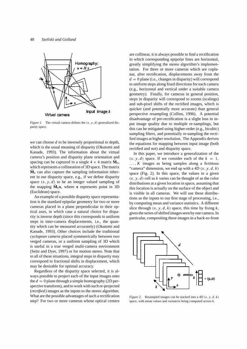
To formulate our (potentially multiframe) stereo prob-lem, we use ageneralized disparity spacewhich canbe any projective sampling of 3D space (Fig. 1). Moreconcretely, we first choose avirtual camerapositionand orientation. This virtual camera may be coincidentwith one of the input images, or it can be chosen basedon the application demands and the desired accuracy ofthe results. For instance, if we wish to regularly sam-ple a volume of 3D space, we can make the cameraorthographic, with the camera’s(x, y, d) axes beingorthogonal and evenly sampled (as in (Seitz and Dyer,1997)). As another example, we may wish to use askewed camera modelfor constructing a Lumigraph(Gortler et al., 1996).

Having chosen a virtual camera position, we canalso choose the orientation and spacing of thedispa-rity planes, i.e., the constantd planes. The relationshipbetweend and 3D space can be projective. For example,


Figure 1. The virtual camera defines the(x, y, d) generalized dis-parity space.

we can choosed to be inversely proportional to depth,which is the usual meaning of disparity (Okutomi andKanade, 1993). The information about the virtualcamera’s position and disparity plane orientation andspacing can be captured in a single 4× 4 matrix M0,which represents a collineation of 3D space. The matrixM0 can also capture the sampling information inher-ent in our disparity space, e.g., if we define disparityspace(x, y, d) to be an integer valued sampling ofthe mappingM0x, where x represents point in 3D(Euclidean) space.

An example of a possible disparity space representa-tion is the standard epipolar geometry for two or morecameras placed in a plane perpendicular to their op-tical axes, in which case a natural choice for dispa-rity is inverse depth (since this corresponds to uniformsteps in inter-camera displacements, i.e., the quan-tity which can be measured accurately) (Okutomi andKanade, 1993). Other choices include the traditionalcyclopean cameraplaced symmetrically between twoverged cameras, or a uniform sampling of 3D whichis useful in a true verged multi-camera environment(Seitz and Dyer, 1997) or for motion stereo. Note thatin all of these situations, integral steps in disparity maycorrespond to fractional shifts in displacement, whichmay be desirable for optimal accuracy.

Regardless of the disparity space selected, it is al-ways possible to project each of the input images ontothed = 0 plane through a simple homography (2D per-spective transform), and to work with such re-projected(rectified) images as the inputs to the stereo algorithm.What are the possible advantages of such a rectificationstep? For two or more cameras whose optical centers

are collinear, it is always possible to find a rectificationin which corresponding epipolar lines are horizontal,greatly simplifying the stereo algorithm’s implemen-tation. For three or more cameras which are copla-nar, after rectification, displacements away from thed = 0 plane (i.e., changes in disparity) will correspondto uniform steps along fixed directions for each camera(e.g., horizontal and vertical under a suitable camerageometry). Finally, for cameras in general position,steps in disparity will correspond to zooms (scalings)and sub-pixel shifts of the rectified images, which isquicker (and potentially more accurate) than generalperspective resampling (Collins, 1996). A potentialdisadvantage of pre-rectification is a slight loss in in-put image quality due to multiple re-samplings, butthis can be mitigated using higher-order (e.g., bicubic)sampling filters, and potentially re-sampling the recti-fied images at higher resolution. The Appendix derivesthe equations for mapping between input image (bothrectified and not) and disparity space.

In this paper, we introduce a generalization of the(x, y, d) space. If we consider each of thek = 1,. . . , K images as being samples along a fictitious“camera” dimension, we end up with a 4D(x, y, d, k)space (Fig. 2). In this space, the values in a given(x, y, d) cell ask varies can be thought of as the colordistributions at a given location in space, assuming thatthis location is actually on the surface of the object andis visible in all cameras. We will use these distribu-tions as the inputs to our first stage of processing, i.e.,by computing mean and variance statistics. A differentslice through(x, y, d, k) space, this time by fixingk,gives the series of shifted images seen by one camera. Inparticular, compositing these images in a back-to-front

Figure 2. Resampled images can be stacked into a 4D(x, y, d, k)space, with mean values and variances being computed acrossk.


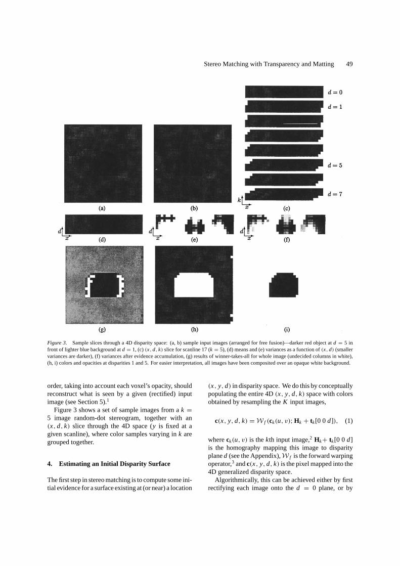
Figure 3. Sample slices through a 4D disparity space: (a, b) sample input images (arranged for free fusion)—darker red object atd = 5 infront of lighter blue background atd = 1, (c)(x, d, k) slice for scanline 17 (k = 5), (d) means and (e) variances as a function of(x, d) (smallervariances are darker), (f) variances after evidence accumulation, (g) results of winner-takes-all for whole image (undecided columns in white),(h, i) colors and opacities at disparities 1 and 5. For easier interpretation, all images have been composited over an opaque white background.

order, taking into account each voxel’s opacity, shouldreconstruct what is seen by a given (rectified) inputimage (see Section 5).1

Figure 3 shows a set of sample images from ak =5 image random-dot stereogram, together with an(x, d, k) slice through the 4D space (y is fixed at agiven scanline), where color samples varying ink aregrouped together.

4. Estimating an Initial Disparity Surface

The first step in stereo matching is to compute some ini-tial evidence for a surface existing at (or near) a location

(x, y, d) in disparity space. We do this by conceptuallypopulating the entire 4D(x, y, d, k) space with colorsobtained by resampling theK input images,

c(x, y, d, k) =W f (ck(u, v);Hk + tk[0 0 d]), (1)

whereck(u, v) is thekth input image,2 Hk+ tk[0 0 d]is the homography mapping this image to disparityplaned (see the Appendix),W f is the forward warpingoperator,3 andc(x, y, d, k) is the pixel mapped into the4D generalized disparity space.

Algorithmically, this can be achieved either by firstrectifying each image onto thed = 0 plane, or by


directly using a homography (planar perspective trans-form) to compute each(d, k) slice.4 Note that at thisstage, not all(x, y, d, k) cells will be populated, assome of these may map to pixels which are outsidesome of the input images.

Once we have a collection of color (or luminance)values at a given(x, y, d) cell, we can compute someinitial statistics over theK (or fewer) colors, e.g., thesample meanµ and varianceσ 2.5 Robust estimatesof sample mean and variance are also possible (e.g.,Scharstein and Szeliski (1996). Examples of the meanand variance values for our sample image are shown inFigs. 3(d) and (e), where darker values indicate smallervariances.

After accumulating the local evidence, we usually donot have enough information to determine the correctdisparities in the scene (unless each pixel has a uniquecolor). While pixels at the correct disparity should intheory have zero variance, this is not true in the presenceof image noise, fractional disparity shifts, and pho-tometric variations (e.g., specularities). The variancemay also be arbitrarily high in occluded regions, wherepixels which actually belong to a different disparitylevel will nevertheless vote, often leading to gross er-rors. For example, in Fig. 3(c), the middle (red) groupof pixels atd = 5 should all have the same color in anygiven column, but they do not because of resamplingerrors. This effect is especially pronounced near theedge of the red square, where the red color has beenseverely contaminated by the background blue. Thiscontamination is one of the reasons why most stereo al-gorithm make systematic errors in the vicinity of depthdiscontinuities.

To help disambiguate matches, we can use local evi-dence aggregation. The most common form is aver-aging using square windows, which results in the tra-ditional sum of squared difference (SSD and SSSD)algorithms (Okutomi and Kanade, 1993). To obtain re-sults with better quality near discontinuities, it is prefer-able to use adaptive windows (Kanade and Okutomi,1994) or iterative evidence accumulation (Scharsteinand Szeliski, 1996). In the latter case, we may wish toaccumulate an evidence measure which is not simplysummed error (e.g., the probability of a correct match(Scharstein and Szeliski, 1996)). Continuing our sim-ple example, Fig. 3(f) shows the results of an evi-dence accumulation stage, where more certain depthsare darker. To generate these results, we aggregate evi-dence using a variant of the algorithm described in

(Scharstein and Szeliski, 1996),

σ t+1i ← aσ t

i + b∑

j∈N4(i )

σ tj + cσ 0

i . (2)

Here,σ 0i is the original variance at pixeli computed

by comparing all sampled colors from thek images,σ t

i is the variance at iterationt , σ ti = min(σ t

i , σmax)

is a robustified (limited) version of the variance, andN4 are the usual four nearest neighbors. The effect ofthis updating rule is todiffusevariance values to theirneighbors, while preventing the diffusion from totallyaveraging out the variances. For the results in Fig. 3,we use(a, b, c) = (0.1, 0.15, 0.3) andσmax= 16.

At this stage, most stereo matching algorithms picka winning disparity in each(x, y) column, and call thisthe final correspondence map. Optionally, they mayalso compute a fractional disparity value by fitting ananalytic curve to the error surface around the winningdisparity and then finding its minimum (Matthies et al.,1989; Okutomi and Kanade, 1993). Unfortunately, thisdoes nothing to resolve several problems: occludedpixels may not be handled correctly (since they have“inconsistent” color values at the correct disparity), andit is difficult to recover the true (unmixed) color valuesof surface elements (or their opacities, in the case ofpixels near discontinuities).

Our solution to this problem is to use the initial dis-parity map as the input to a refinement stage whichsimultaneously estimates the disparities, colors, andopacities which best match the input images while con-forming to some prior expectations on smoothness. Tostart this procedure, we initially pick only winners ineach column where the answer is fairly certain, i.e.,where the variance (“scatter” in color values) is belowa threshold and is a clear winner with respect to theother candidate disparities.6 A new(x, y, d) volume iscreated, where each cell now contains a color value, ini-tially set to the mean color computed in the first stage,and the opacity is set to 1 for cells which are winners,and 0 otherwise.7

5. Computing Visibilities Through Re-Projection

Once we have an initial(x, y, d) volume containingestimated RGBA (color and 0/1 opacity) values, we canre-project this volume into each of the input camerasusing the known transformation

xk = M kM−10 x0 (3)


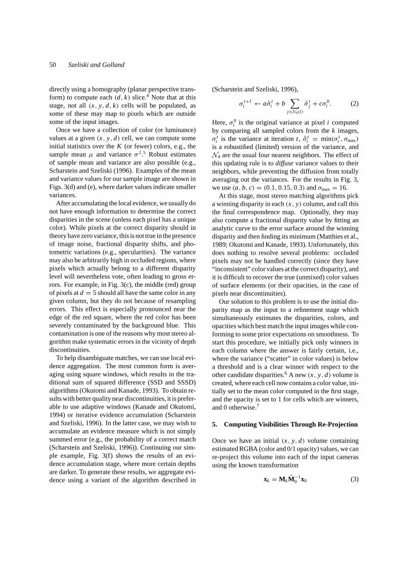
Figure 4. “Stack of acetates” model for image formation from(x, y, d) RGBA color/opacity volume.

(see (A1) in the Appendix), wherex0 is a (homoge-neous) coordinate in(x, y, d) space,M0 is the com-plete camera matrix corresponding to the virtualcamera,M k is thekth camera matrix, andxk are theimage coordinates in thekth image. There are severaltechniques possible for performing this projection, in-cluding classicalvolume renderingtechniques (Levoy,1990; Lacroute and Levoy, 1994). In our approach,we interpret the(x, y, d) volume as a set of (poten-tially) transparent acetates stacked at differentd levels(Fig. 4). Each acetate is first warped into a given inputcamera’s frame using the known homography

xk = Hkx0+ tkd = (Hk + tk[0 0 d]) x0 (4)

wherex0 = (x, y, 1), and the layers are then compo-sited back-to-front (this is called a shear-warp algo-rithm (Lacroute and Levoy, 1994)).8

The resampling procedure for a given layerd intothe coordinate system of camerak can be written as

ck(u, v,d) =Wb(c(x, y, d);Hk + tk[0 0 d]), (5)

wherec = [r g b α]T is the current color and opacityestimate at a given location(x, y, d), ck is the resam-pled layerd in camerak’s coordinate system, andWb isthe resampling operation induced by the homography(4).9 The opacity valueα is 0 for transparent pixels,1 for opaque pixels, and in between for border pixels.Note that the warping function islinear in the colorsand opacities being resampled, i.e., theck(u, v,d) canbe expressed as a linear function of thec(x, y, d), e.g.,through a sparse matrix multiplication.

Once the layers have been resampled, they are thencomposited using the standardover operator (Porterand Duff, 1984),

f ¯ b ≡ f + (1− α f )b,

where f and b are the premultiplied foreground andbackground colors, andα f is the opacity of the fore-ground (Porter and Duff, 1984; Blinn, 1994a). Notethat for α f = 0 (transparent foreground), the back-ground is selected, whereas forα f = 1 (opaque fore-ground), the foreground is returned. Using the overoperator, we can form a composite image

ck(u, v)=dmin⊙

d=dmax

ck(u, v,d)

= ck(u, v,dmax)¯ · · · ¯ ck(u, v,dmin) (6)

(note that the over operator is associative but not com-mutative, and thatdmax is the layer closest to thecamera).

After the re-projection step, we refine the disparityestimates by preventing visible surface pixels from vot-ing for potential disparities in the regions they occlude.More precisely, we build an(x, y, d, k) visibility map,which indicates whether a given camerak can see avoxel at location(x, y, d). A simple way to constructsuch a visibility map is to record the disparity valuedtop

for each(u, v) pixel which corresponds to the topmostopaque pixel seen during the compositing step.10 Thevisibility value can then be defined as

Vk(u, v,d) = if d ≥ dtop(u, v) then 1 else 0.

The visibility and opacity (alpha) values taken togethercan be interpreted as follows:

Vk = 1, ak = 0: free spaceVk = 1, ak = 1: surface voxel visible in imagekVk = 0, ak = ?: voxel not visible in imagek

whereak is the opacity ofck in (5).A more principled way of defining visibility, which

takes into account partially opaque voxels, uses a re-cursive front-to-back algorithm

Vk(u, v,d − 1)=Vk(u, v,d) (1− ak(u, v,d))

=dmax∏d′=d

(1− ak(u, v,d′)), (7)


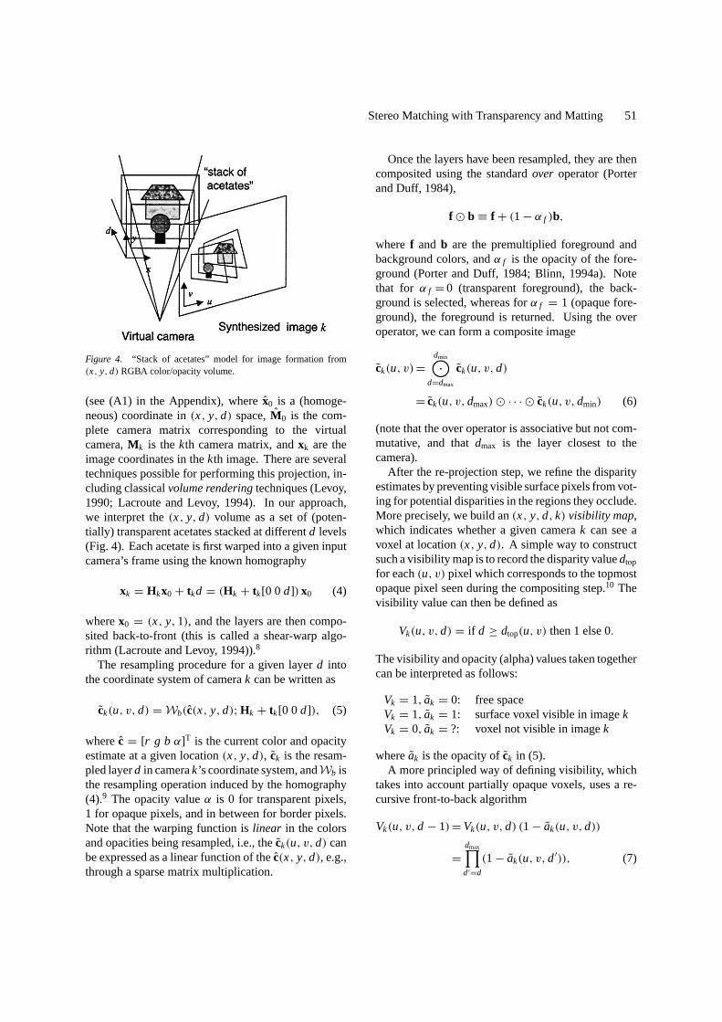
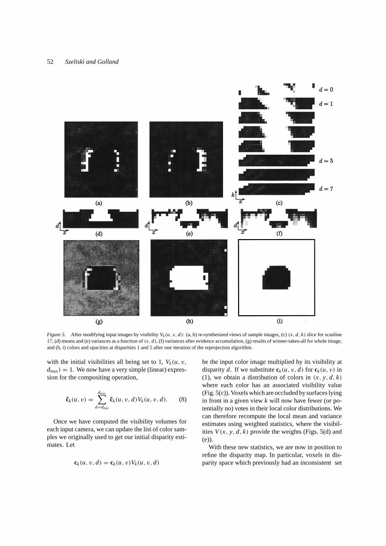
Figure 5. After modifying input images by visibilityVk(u, v,d): (a, b) re-synthesized views of sample images, (c)(x, d, k) slice for scanline17, (d) means and (e) variances as a function of(x, d), (f) variances after evidence accumulation, (g) results of winner-takes-all for whole image,and (h, i) colors and opacities at disparities 1 and 5 after one iteration of the reprojection algorithm.

with the initial visibilities all being set to 1,Vk(u, v,dmax) = 1. We now have a very simple (linear) expres-sion for the compositing operation,

ck(u, v) =dmax∑

d=dmin

ck(u, v,d)Vk(u, v,d). (8)

Once we have computed the visibility volumes foreach input camera, we can update the list of color sam-ples we originally used to get our initial disparity esti-mates. Let

ck(u, v,d) = ck(u, v)Vk(u, v,d)

be the input color image multiplied by its visibility atdisparityd. If we substituteck(u, v,d) for ck(u, v) in(1), we obtain a distribution of colors in(x, y, d, k)where each color has an associated visibility value(Fig. 5(c)). Voxels which are occluded by surfaces lyingin front in a given viewk will now have fewer (or po-tentially no) votes in their local color distributions. Wecan therefore recompute the local mean and varianceestimates using weighted statistics, where the visibil-ities V(x, y, d, k) provide the weights (Figs. 5(d) and(e)).

With these new statistics, we are now in position torefine the disparity map. In particular, voxels in dis-parity space which previously had an inconsistent set


of color votes (large variance) may now have a con-sistent set of votes, because voxels in (partially oc-cluded) regions will now only receive votes from inputpixels which are not already assigned to nearer surfaces(Figs. 5(c)–(f)). Figure 5(g)–(i) show the results afterone iteration of this algorithm.

6. Refining Color and Transparency Estimates

While the above process of computing visibilities andrefining disparity estimates will in general lead to ahigher quality disparity map (and better quality meancolors, i.e., texture maps), it will not recover the truecolors and transparencies inmixed pixels, e.g., neardepth discontinuities, which is one of the main goalsof this research.

A simple way to approach this problem is to take thebinary opacity maps produced by our stereo matchingalgorithm, and to make them real-valued using a low-pass filter. Another possibility might be to recover thetransparency information by looking at the magnitudeof the intensity gradient (Mitsunaga et al., 1995), as-suming that we can isolate regions which belong todifferent disparity levels.

In our work, we have chosen instead to adjust theopacity and color valuesc(x, y, d) to match the inputimages (after re-projection), while favoring continuityin the color and opacity values. This can be formulatedas a non-linear minimization problem, where the costfunction has three parts:

1. a weighted error norm on the difference betweenthe re-projected imagesck(u, v)and the original (orrectified) input imagesck(u, v)

C1 =∑(u,v)

wk(u, v)ρ1(ck(u, v)− ck(u, v)), (9)

where the weightswk(u, v) may depend on theposition of camerak relative to the virtual cam-era;11

2. a (weak) smoothness constraint on the colors andopacities,

C2=∑(x,y,d)

∑(x′,y′,d′)∈N (x,y,d)

ρ2(c(x′, y′, d′)− c(x, y, d));

(10)

3. a prior distribution on the opacities,

C3 =∑(x,y,d)

φ(α(x, y, d)). (11)

In the above equations,ρ1 andρ2 are either quadraticfunctions or robust penalty functions (Huber, 1981),andφ is a function which encourages opacities to be 0or 1, e.g.,φ(x) = x(1− x).12

The smoothness constraint on colors makes moresense with non-premultiplied colors. For example, avoxel lying on a depth discontinuity will be partiallytransparent, and yet should have the same non-premu-ltiplied color as its neighbors. An alternative, whichallows us to work with premultiplied colors, is to use asmoothness constraint of the form

C ′2 =∑(x,y,d)

∑(x′,y′,d′)∈N (x,y,d)

ρ2(D) (12)

where

D = α(x, y, d)c(x′, y′, d′)− α(x′, y′, d′)c(x, y, d).

To minimize the total cost function

C = λ1C1+ λ2C2+ λ3C3, (13)

we use a preconditioned gradient descent algorithm.The Appendix contains details on how to compute therequired gradients and Hessians.

7. Experiments

To study the properties of our new stereo correspon-dence algorithm, we ran a small set of experiments onsome synthetic stereo datasets, both to evaluate the ba-sic behavior of the algorithm (aggregation, visibility-based refinement, and energy minimization), and tostudy its performance on mixed (boundary) pixels. Be-ing able to visualize opacities/transparencies is veryimportant for understanding and validating our algo-rithm. For this reason, we chose color stimuli (the back-ground is blue-green, and the foreground is red). Pixelswhich are partially transparent will show up as “pale”colors, while fully transparent pixels will be white. Weshould emphasize that our algorithm does not requirecolored images as inputs (see Fig. 8), nor does it requirethe use of standard epipolar geometries.


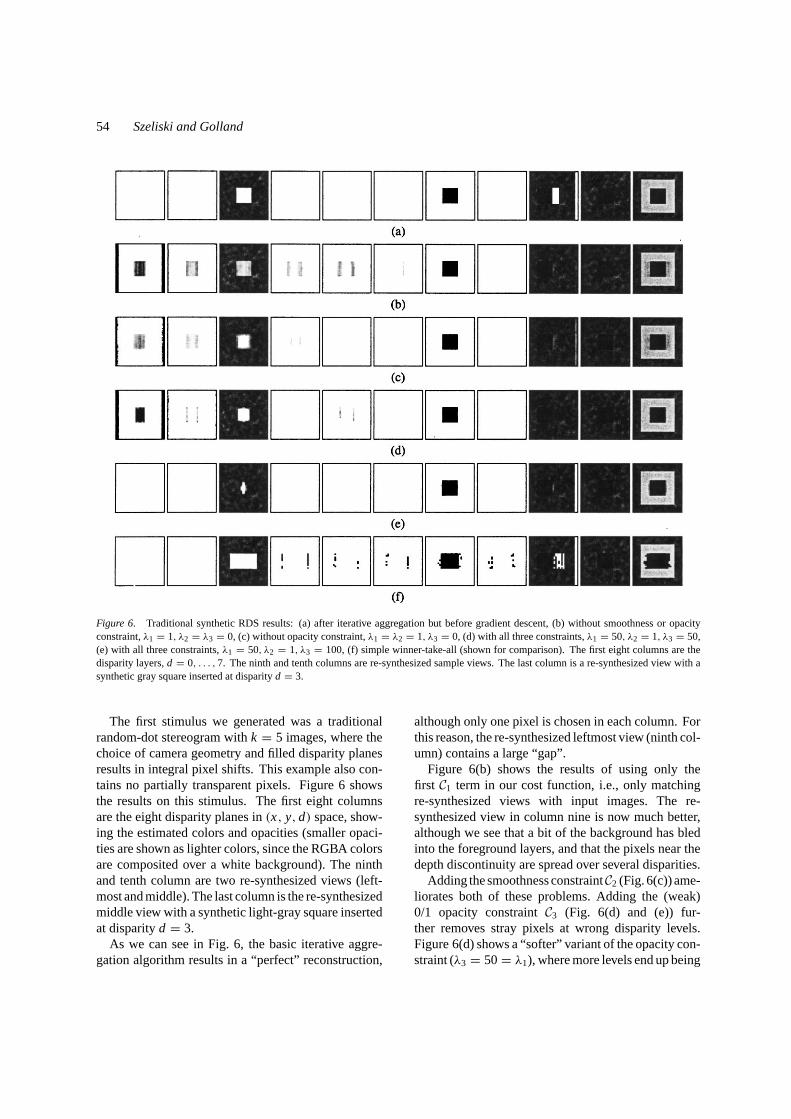
Figure 6. Traditional synthetic RDS results: (a) after iterative aggregation but before gradient descent, (b) without smoothness or opacityconstraint,λ1 = 1, λ2 = λ3 = 0, (c) without opacity constraint,λ1 = λ2 = 1, λ3 = 0, (d) with all three constraints,λ1 = 50, λ2 = 1, λ3 = 50,(e) with all three constraints,λ1 = 50, λ2 = 1, λ3 = 100, (f) simple winner-take-all (shown for comparison). The first eight columns are thedisparity layers,d = 0, . . . ,7. The ninth and tenth columns are re-synthesized sample views. The last column is a re-synthesized view with asynthetic gray square inserted at disparityd = 3.

The first stimulus we generated was a traditionalrandom-dot stereogram withk = 5 images, where thechoice of camera geometry and filled disparity planesresults in integral pixel shifts. This example also con-tains no partially transparent pixels. Figure 6 showsthe results on this stimulus. The first eight columnsare the eight disparity planes in(x, y, d) space, show-ing the estimated colors and opacities (smaller opaci-ties are shown as lighter colors, since the RGBA colorsare composited over a white background). The ninthand tenth column are two re-synthesized views (left-most and middle). The last column is the re-synthesizedmiddle view with a synthetic light-gray square insertedat disparityd = 3.

As we can see in Fig. 6, the basic iterative aggre-gation algorithm results in a “perfect” reconstruction,

although only one pixel is chosen in each column. Forthis reason, the re-synthesized leftmost view (ninth col-umn) contains a large “gap”.

Figure 6(b) shows the results of using only thefirst C1 term in our cost function, i.e., only matchingre-synthesized views with input images. The re-synthesized view in column nine is now much better,although we see that a bit of the background has bledinto the foreground layers, and that the pixels near thedepth discontinuity are spread over several disparities.

Adding the smoothness constraintC2 (Fig. 6(c)) ame-liorates both of these problems. Adding the (weak)0/1 opacity constraintC3 (Fig. 6(d) and (e)) fur-ther removes stray pixels at wrong disparity levels.Figure 6(d) shows a “softer” variant of the opacity con-straint (λ3 = 50= λ1), where more levels end up being


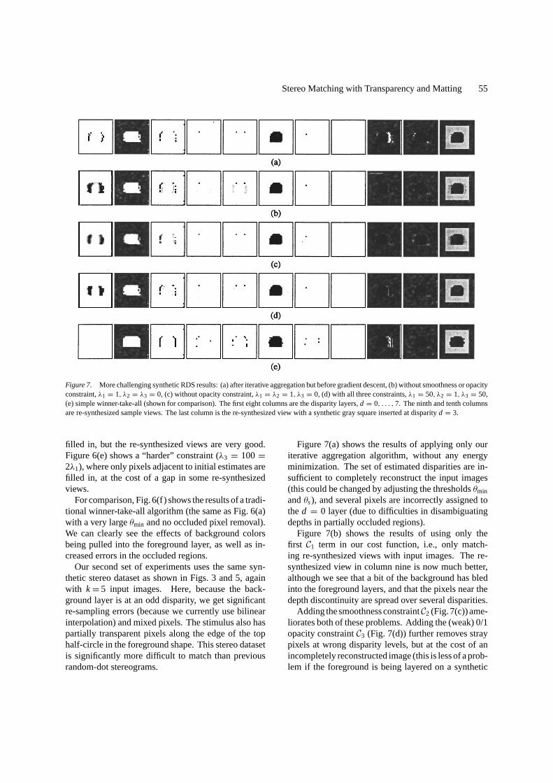
Figure 7. More challenging synthetic RDS results: (a) after iterative aggregation but before gradient descent, (b) without smoothness or opacityconstraint,λ1 = 1, λ2 = λ3 = 0, (c) without opacity constraint,λ1 = λ2 = 1, λ3 = 0, (d) with all three constraints,λ1 = 50, λ2 = 1, λ3 = 50,(e) simple winner-take-all (shown for comparison). The first eight columns are the disparity layers,d = 0, . . . ,7. The ninth and tenth columnsare re-synthesized sample views. The last column is the re-synthesized view with a synthetic gray square inserted at disparityd = 3.

filled in, but the re-synthesized views are very good.Figure 6(e) shows a “harder” constraint (λ3 = 100=2λ1), where only pixels adjacent to initial estimates arefilled in, at the cost of a gap in some re-synthesizedviews.

For comparison, Fig. 6(f) shows the results of a tradi-tional winner-take-all algorithm (the same as Fig. 6(a)with a very largeθmin and no occluded pixel removal).We can clearly see the effects of background colorsbeing pulled into the foreground layer, as well as in-creased errors in the occluded regions.

Our second set of experiments uses the same syn-thetic stereo dataset as shown in Figs. 3 and 5, againwith k= 5 input images. Here, because the back-ground layer is at an odd disparity, we get significantre-sampling errors (because we currently use bilinearinterpolation) and mixed pixels. The stimulus also haspartially transparent pixels along the edge of the tophalf-circle in the foreground shape. This stereo datasetis significantly more difficult to match than previousrandom-dot stereograms.

Figure 7(a) shows the results of applying only ouriterative aggregation algorithm, without any energyminimization. The set of estimated disparities are in-sufficient to completely reconstruct the input images(this could be changed by adjusting the thresholdsθmin

andθs), and several pixels are incorrectly assigned tothed = 0 layer (due to difficulties in disambiguatingdepths in partially occluded regions).

Figure 7(b) shows the results of using only thefirst C1 term in our cost function, i.e., only match-ing re-synthesized views with input images. The re-synthesized view in column nine is now much better,although we see that a bit of the background has bledinto the foreground layers, and that the pixels near thedepth discontinuity are spread over several disparities.

Adding the smoothness constraintC2 (Fig. 7(c)) ame-liorates both of these problems. Adding the (weak) 0/1opacity constraintC3 (Fig. 7(d)) further removes straypixels at wrong disparity levels, but at the cost of anincompletely reconstructed image (this is less of a prob-lem if the foreground is being layered on a synthetic


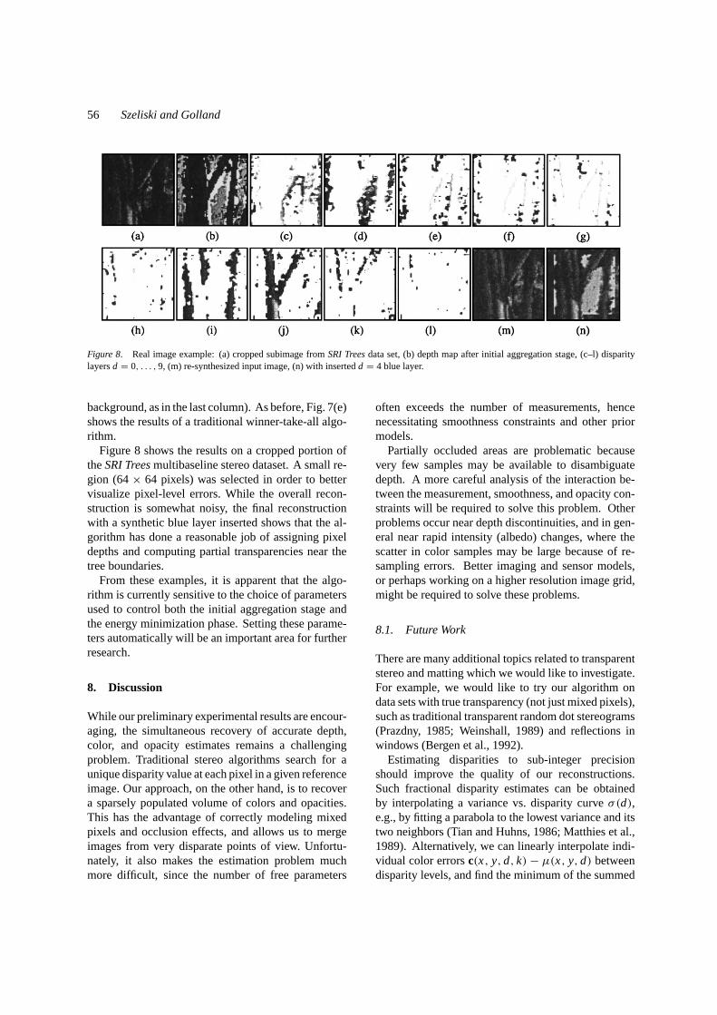
Figure 8. Real image example: (a) cropped subimage fromSRI Treesdata set, (b) depth map after initial aggregation stage, (c–l) disparitylayersd = 0, . . . ,9, (m) re-synthesized input image, (n) with insertedd = 4 blue layer.

background, as in the last column). As before, Fig. 7(e)shows the results of a traditional winner-take-all algo-rithm.

Figure 8 shows the results on a cropped portion oftheSRI Treesmultibaseline stereo dataset. A small re-gion (64× 64 pixels) was selected in order to bettervisualize pixel-level errors. While the overall recon-struction is somewhat noisy, the final reconstructionwith a synthetic blue layer inserted shows that the al-gorithm has done a reasonable job of assigning pixeldepths and computing partial transparencies near thetree boundaries.

From these examples, it is apparent that the algo-rithm is currently sensitive to the choice of parametersused to control both the initial aggregation stage andthe energy minimization phase. Setting these parame-ters automatically will be an important area for furtherresearch.

8. Discussion

While our preliminary experimental results are encour-aging, the simultaneous recovery of accurate depth,color, and opacity estimates remains a challengingproblem. Traditional stereo algorithms search for aunique disparity value at each pixel in a given referenceimage. Our approach, on the other hand, is to recovera sparsely populated volume of colors and opacities.This has the advantage of correctly modeling mixedpixels and occlusion effects, and allows us to mergeimages from very disparate points of view. Unfortu-nately, it also makes the estimation problem muchmore difficult, since the number of free parameters

often exceeds the number of measurements, hencenecessitating smoothness constraints and other priormodels.

Partially occluded areas are problematic becausevery few samples may be available to disambiguatedepth. A more careful analysis of the interaction be-tween the measurement, smoothness, and opacity con-straints will be required to solve this problem. Otherproblems occur near depth discontinuities, and in gen-eral near rapid intensity (albedo) changes, where thescatter in color samples may be large because of re-sampling errors. Better imaging and sensor models,or perhaps working on a higher resolution image grid,might be required to solve these problems.

8.1. Future Work

There are many additional topics related to transparentstereo and matting which we would like to investigate.For example, we would like to try our algorithm ondata sets with true transparency (not just mixed pixels),such as traditional transparent random dot stereograms(Prazdny, 1985; Weinshall, 1989) and reflections inwindows (Bergen et al., 1992).

Estimating disparities to sub-integer precisionshould improve the quality of our reconstructions.Such fractional disparity estimates can be obtainedby interpolating a variance vs. disparity curveσ(d),e.g., by fitting a parabola to the lowest variance and itstwo neighbors (Tian and Huhns, 1986; Matthies et al.,1989). Alternatively, we can linearly interpolate indi-vidual color errorsc(x, y, d, k) − µ(x, y, d) betweendisparity levels, and find the minimum of the summed


squared error (which will be a quadratic function of thefractional disparity).

Instead of representing our color volumec(x, y, d)using colors pre-multiplied by their opacities (Blinn,1994a), we could keep these quantities separate. Thus,colors could “bleed” into areas which are transparent,which may be a more natural representation for colorsmoothness (e.g., for surfaces with small holes). Dif-ferent color representations such as hue, saturation, in-tensity (HSV) may also be more suitable for performingcorrespondence (Golland and Bruckstein, 1995), andthey would permit us to reason more directly about un-derlying physical processes (shadows, shading, etc.).

In recent work, we have extended our stack of ace-tates model to use a smaller number of tilted acetateswith arbitrary plane equations (Baker et al., 1998). Thiswork is closely related to more traditional layered mo-tion models (Wang and Adelson, 1993; Ju et al., 1996;Sawhney and Ayer, 1996; Weiss and Adelson, 1996),but focuses on recovering 3D descriptions instead of2D motion estimates. Each layer can also have an ar-bitrary out-of plane parallax component (Baker et al.,1998). The layers are thus used to represent the grossshape and occlusion relationships, while the parallaxencodes the fine shape variation. We are also inves-tigating efficient rendering algorithm for doing viewsynthesis from suchsprites with depth(Shade et al.,1998).

9. Conclusions

In this paper, we have developed a new frameworkfor simultaneously recovering disparities, colors, andopacities from multiple images. This framework en-ables us to deal with many commonly occurringproblems in stereo matching, such as partially oc-cluded regions and pixels which contain mixtures offoreground and background colors. Furthermore, itpromises to deliver better quality (sub-pixel accurate)color and opacity estimates, which can be used for fore-ground object extraction and mixing live and syntheticimagery.

To set the problem in as general a framework as pos-sible, we have introduced the notion of a virtual camerawhich defines a generalized disparity space, which canbe any regular projective sampling of 3D. We representthe output of our algorithm as a collection of color andopacity values lying on this sampled grid. Any inputimage can (in principle) be re-synthesized by warp-ing each disparity layer using a simple homography

and compositing the images. This representation cansupport a much wider range of synthetic viewpoints inview interpolation applications than a single texture-mapped depth image.

To solve the correspondence problem, we first com-pute mean and variance estimates at each cell in our(x, y, d) grid. We then pick a subset of the cells whichare likely to lie on the reconstructed surface usinga thresholded winner-take-all scheme. The mean andvariance estimates are then refined by removing fromconsideration cells which are in the occluded (shadow)region of each current surface element, and this processis repeated.

Starting from this rough estimate, we formulate anenergy minimization problem consisting of an inputmatching criterion, a smoothness criterion, and a prioron likely opacities. This criterion is then minimizedusing an iterative preconditioned gradient descent al-gorithm.

While our preliminary experimental results look en-couraging, there remains much work to be done indeveloping truly accurate and robust correspondencealgorithms. We believe that the development of suchalgorithms will be crucial in promoting a wider use ofstereo-based imaging in novel applications such as spe-cial effects, virtual reality modeling, and virtual studioproductions.

Appendix

Camera Models, Disparity Space,and Induced Homographies

The homographies mapping input images (rectified ornot) to planes in disparity space can be derived directlyfrom the camera matrices involved. Throughout thisappendix, we use projective coordinates, i.e., equalityis defined only up to a scale factor.

Let M k be the 3× 4 camera matrixwhich mapsreal-world coordinatesx = [X Y Z 1]T into a cam-era’s screen coordinatesxk = [u v 1]T, xk = M kx.Similarly, letM0 be the 4× 4 collineation which mapsworld coordinatesx into disparity space coordinatesx0 = [x y 1 d]T, x0 = M0x.

We can write the mapping between a pixel in thedthdisparity plane,x0 = [x y 1]T, and its correspondingcoordinatexk in thekth input image as

xk = M kM−10 x0 = Hkx0+ tkd

= (Hk + tk[0 0 d]) x0, (A1)


whereHk is the homography relating the rectified andnon-rectified version of input imagek (i.e., the homo-graphy ford= 0), andtk is the image of the virtualcamera’s center of projection in imagek, i.e., theepipole (this can be seen by settingd→∞).

If we first rectify an input image, we can re-projectit into a new disparity planed using

xk = Hkx′0 = Hkx0+ tkd

wherex′0 is the new coordinate corresponding tox0 atd = 0. From this,

x′0 = x0+ tkd = (I + tk[0 0 d])x0 = Hkx0,

wheretk = H−1k tk is the focus of expansion, and the

new homographyHk = I + tk[0 0 d] represents a sim-ple shift and scale. It can be shown (Collins, 1996) thatthe first two elements oftk depend on the horizontaland vertical displacements between the virtual cameraand thekth camera, whereas the third element is pro-portional to the displacement in depth (perpendicularto thed plane). Thus, if all of the cameras are coplanar(regardless of their vergence), and if thed planes areparallel to this common plane, then the re-mappings ofrectified images to a new disparity correspond to pureshifts.

Note that in the body of the paper, when we speak ofthe homography (A1) parameterized byHk andtk, wecan replaceHk and tk by I and tk if the input imageshave been pre-rectified.

Gradient Descent Algorithm

To implement our gradient descent algorithm, we needto compute the partial derivatives of the cost functionsC1, . . . , C3 with respect to all of the unknowns, i.e., thecolors and opacitiesc(x, y, d). In this section, we willusec= [r g bα]T to indicate the four-element vector ofcolors and opacities, andα to indicate just the opacitychannel. In addition to computing the partial deriva-tives, we will compute the diagonal of the approximateHessian matrix (Press et al., 1992, pp. 681–685), i.e.,the square of the derivative of the term inside theρfunction.

The derivative ofC1 given in (9) can be computed byfirst expressingck(u, v) in terms ofck(u, v,d),

ck(u, v) =dmax∑

d=dmin

ck(u, v,d)Vk(u, v,d)

=dmax∑d′=d

ck(u, v,d′)Vk(u, v,d

′)

+ (1− αk(u, v,d))ak(u, v,d − 1),

where

ak(u, v,d) =d∑

d′=dmin

ck(u, v,d′)Vk(u, v,d

′)

is the accumulated color/opacityin layer d, withck(u, v) = ak(u, v,dmax). We obtain

∂rk(u, v)

∂rk(u, v,d)= ∂gk(u, v)

∂gk(u, v,d)= ∂bk(u, v)

∂bk(u, v,d)

= Vk(u, v,d)

and

∂ ck(u, v)

∂αk(u, v,d)= [0 0 0 Vk(u, v,d)]

T − ak(u, v,d− 1).

Let ek(u, v) = ck(u, v)− ck(u, v) be the color error inimagek, and assume for now thatwk = 1 andρ1(ek) =‖ek‖2 in (9). The gradient ofC1 w.r.t. ck(u, v,d) is thus

gk(u, v,d) = Vk(u, v,d)(ek(u, v)

− [0 0 0ek(u, v) · ak(u, v,d − 1)]T)

while the diagonal of the Hessian is

hk(u, v,d) = Vk(u, v,d)

× [1 1 1 1− ‖ak(u, v,d − 1)‖2]T.

Once we have computed the derivatives w.r.t. thewarpedpredicted color valuesck(u, v,d), we need toconvert this to the gradient w.r.t. the disparity spacecolorsc(x, y, d). This can be done using the transposeof the linear mapping induced by the backward warpWb used in (5). For certain cases (pure shifts), this is thesame as warping the gradientgk(u, v,d) and Hessianhk(u, v,d) through the forward warpW f ,

g1(x, y, d, k) = W f (gk(u, v,d);Hk + tk[0 0 d]),

h1(x, y, d, k) = W f ( hk(u, v,d);Hk + tk[0 0 d]).

For many other cases (moderate scaling and shear), thisis still a good approximation, so it is the approach wecurrently use.


Computing the gradient ofC2 w.r.t. c(x, y, d) ismuch more straightforward,

g2(x, y, d) =∑

(x′,y′,d′)∈N4(x,y,d)

ρ2(c(x′, y′, d′)− c(x, y, d)),

whereρ2 is applied to each color component separately.The Hessian will be a constant for a quadratic penaltyfunction; for a non-quadratic function, the secant ap-proximationρ(r )/r can be used (Sawhney and Ayer,1996).

Finally, the derivative of the opacity penalty functionC3 can easily be computed forφ = x(1− x),

g3(x, y, d) = [0 0 0 (1− 2α(x, y, d))]T.

To ensure that the Hessian is positive, we seth3(x,y, d) = [0 0 0 1]T.

The gradients for the three cost functions can nowbe combined

g(x, y, d) = λ1

K∑k=1

g1(x, y, d, k)+ λ2g2(x, y, d)

+ λ3g3(x, y, d),

h(x, y, d) = λ1

K∑k=1

h1(x, y, d, k)+ λ2 h2(x, y, d)

+ λ3 h3(x, y, d),

and a gradient descent step can be performed,

c(x, y, d)← c(x, y, d)+ ε1g(x, y, d)/

( h(x, y, d)+ ε2). (A2)

In our current experiments, we useε1 = ε2 = 0.5.13

Notes

1. Note that this 4D space isnot the same as that used in the Lumi-graph (Gortler et al., 1996), where the description is one of raysin 3D, as opposed to color distributions across multiple camerasin 3D. It is also not the same as an epipolar-plane image (EPI)volume (Bolles et al., 1987), which is a simple concatenation ofwarped input images.

2. The color valuesc can be replaced with gray-level intensityvalues without affecting the validity of our analysis.

3. In our current implementation, the warping (resampling) algo-rithm uses bi-linear interpolation of the pixel colors and opaci-ties.

4. For certain epipolar geometries, even more efficient algorithmsare possible, e.g., by simply shifting along epipolar lines(Kanade et al., 1996).

5. In many traditional stereo algorithms, it is common to effectivelyset the mean to be just the value in one image, which makes thesealgorithms not truly multiframe (Collins, 1996). The samplevariance then corresponds to the squared difference or sum ofsquared differences (Okutomi and Kanade, 1993).

6. To account for resampling errors which occur near rapid coloror luminance changes, we set the threshold proportional to thelocal image variation within a 3× 3 window, Var3×3. In ourexperiments, the threshold is set toθ = θmin + θsVar3×3, withθmin = 10 andθs = 0.02.

7. We may, for computational reasons, choose to represent thisvolume using colors premultiplied by their opacities (associatedcolors (Porter and Duff, 1984; Blinn, 1994a)), in which casevoxels for which alpha (opacity) is 0 should have their coloror intensity values set to 0. See Blinn (1994a, 1994b) for adiscussion of the advantages of using premultiplied colors.

8. If the input images have been rectified, or under certain imaginggeometries, this homography will be a simple scale and/or shift(see the Appendix).

9. This is the inverse of the warp specified in (1).10. Note that it is not possible to compute visibility in(x, y, d)

disparity space, as several opaque pixels in disparity space maypotentially project to the same input camera pixel.

11. More precisely, we may wish to measure the angle betweenthe viewing ray corresponding to(u, v) in the two cameras.However, the ray corresponding to(u, v) in the virtual cameradepends on the disparityd.

12. All color and opacity values are, of course, constrained to lie inthe range [0, 1], making this a constrained optimization prob-lem.

13. A more sophisticated Levenberg-Marquardt minimizationtechnique could also be implemented by adding an extrastabilization parameter (Press et al., 1992). However, imple-menting a full Levenberg-Marquardt with off-diagonal Hessianelements would greatly complicate the implementation.

References

Adelson, E.H. and Anandan, P. 1990. Ordinal characteristics oftransparency. InAAAI-90 Workshop on Qualitative Vision, AAAI:Boston, MA, pp. 77–81.

Adelson, E.H. and Anandan, P. 1993. Perceptual organization andthe judgement of brightness.Science, 262:2042–2044.

Arnold, R.D. 1983. Automated stereo perception. Technical ReportAIM-351, Artificial Intelligence Laboratory, Stanford University.

Baker, H.H. 1980. Edge based stereo correlation. InImage Under-standing Workshop, L.S. Baumann (Ed.), Science ApplicationsInternational Corporation, pp. 168–175.

Baker, S., Szeliski, R., and Anandan, P. 1998. A layered approachto stereo reconstruction. InIEEE Computer Society Conferenceon Computer Vision and Pattern Recognition (CVPR’98), SantaBarbara.

Barnard, S.T. 1989. Stochastic stereo matching over scale.Interna-tional Journal of Computer Vision, 3(1):17–32.

Barnard, S.T. and Fischler, M.A. 1982. Computational stereo.Com-puting Surveys, 14(4):553–572.


Belhumeur, P.N. and Mumford, D. 1992. A Bayesian treatment ofthe stereo correspondence problem using half-occluded regions.In Computer Vision and Pattern Recognition, Champaign-Urbana,Illinois, pp. 506–512.

Bergen, J.R., Burt, P.J., Hingorani, R., and Peleg, S. 1992. A three-frame algorithm for estimating two-component image motion.IEEE Transactions on Pattern Analysis and Machine Intelligence,14(9):886–896.

Blinn, J.F. 1994a. Jim Blinn’s corner: Compositing, part 1: Theory.IEEE Computer Graphics and Applications, 14(5):83–87.

Blinn, J.F. 1994b. Jim Blinn’s corner: Compositing, part 2: Practice.IEEE Computer Graphics and Applications, 14(6):78–82.

Blonde, L. et al. 1996. A virtual studio for live broadcasting: TheMona Lisa project.IEEE Multimedia, 3(2):18–29.

Bolles, R.C., Baker, H.H., and Marimont, D.H. 1987. Epipolar-planeimage analysis: An approach to determining structure from mo-tion. International Journal of Computer Vision, 1:7–55.

Collins, R.T. 1996. A space-sweep approach to true multi-imagematching. InIEEE Computer Society Conference on ComputerVision and Pattern Recognition (CVPR’96), San Francisco, Cali-fornia, pp. 358–363.

Cox, I.J. 1994. A maximum likelihood n-camera stereo algorithm.In IEEE Computer Society Conference on Computer Vision andPattern Recognition (CVPR’94), IEEE Computer Society: Seattle,Washington, pp. 733–739.

Darrell, T. and Pentland, A. 1991. Robust estimation of a multi-layered motion representation. InIEEE Workshop on VisualMotion, IEEE Computer Society Press: Princeton, New Jersey,pp. 173–178.

Dhond, U.R. and Aggarwal, J.K. 1989. Structure from stereo—Areview. IEEE Transactions on Systems, Man, and Cybernetics,19(6):1489–1510.

Fua, P. 1993. A parallel stereo algorithm that produces dense depthmaps and preserves image features.Machine Vision and Applica-tions, 6:35–49.

Geiger, D., Ladendorf, B., and Yuille, A. 1992. Occlusions andbinocular stereo. InSecond European Conference on ComputerVision (ECCV’92), Springer-Verlag: Santa Margherita Liguere,Italy, pp. 425–433.

Golland, P. and Bruckstein, A. 1995. Motion from color. TechnicalReport 9513, IS Lab, CS Department, Technion, Haifa, Israel.

Gortler, S.J., Grzeszczuk, R., Szeliski, R., and Cohen, M.F. 1996.The lumigraph. InComputer Graphics Proceedings, Annual Con-ference Series, ACM SIGGRAPH, Proc. SIGGRAPH’96 (NewOrleans), pp. 43–54.

Huber, P.J. 1981.Robust Statistics. John Wiley & Sons: New York.Intille, S.S. and Bobick, A.F. 1994. Disparity-space images and large

occlusion stereo. InProc. Third European Conference on Com-puter Vision (ECCV’94), Springer-Verlag: Stockholm, Sweden.

Jenkin, M.R.M., Jepson, A.D., and Tsotsos, J.K. 1991. Tech-niques for disparity measurement.CVGIP: Image Understanding,53(1):14–30.

Jones, D.G. and Malik, J. 1992. A computational framework for de-termining stereo correspondence from a set of linear spatial filters.In Second European Conference on Computer Vision (ECCV’92),Springer-Verlag: Santa Margherita Liguere, Italy, pp. 397–410.

Ju, S.X., Black, M.J., and Jepson, A.D. 1996. Skin and bones:Multi-layer, locally affine, optical flow and regularization withtransparency. InIEEE Computer Society Conference on Com-

puter Vision and Pattern Recognition (CVPR’96), San Francisco,California, pp. 307–314.

Kanade, T. and Okutomi, M. 1994. A stereo matching algorithm withan adaptive window: Theory and experiment.IEEE Transactionson Pattern Analysis and Machine Intelligence, 16(9):920–932.

Kanade, T., Yoshida, A., Oda, K., Kano, H., and Tanaka, M. 1996.A stereo machine for video-rate dense depth mapping and its newapplications. InIEEE Computer Society Conference on ComputerVision and Pattern Recognition (CVPR’96), San Francisco, Cali-fornia, pp. 196–202.

Kang, S.B., Webb, J., Zitnick, L., and Kanade, T. 1995. A multi-baseline stereo system with active illumination and real-time im-age acquisition. InFifth International Conference on ComputerVision (ICCV’95), Cambridge, Massachusetts, pp. 88–93.

Lacroute, P. and Levoy, M. 1994. Fast volume rendering using ashear-warp factorization of the viewing transformation.ComputerGraphics (SIGGRAPH’94), 451–457.

Levoy, M. 1990. Efficient ray tracing of volume data.ACM Trans-actions on Graphics, 9(3):245–261.

Lucas, B.D. and Kanade, T. 1981. An iterative image registrationtechnique with an application in stereo vision. InSeventh Inter-national Joint Conference on Artificial Intelligence (IJCAI-81),Vancouver, pp. 674–679.

Marr, D. and Poggio, T. 1976. Cooperative computation of stereodisparity.Science, 194:283–287.

Matthies, L.H., Szeliski, R., and Kanade, T. 1989. Kalman filter-based algorithms for estimating depth from image sequences.In-ternational Journal of Computer Vision, 3:209–236.

McMillan, L. and Bishop, G. 1995. Plenoptic modeling: An image-based rendering system.Computer Graphics (SIGGRAPH’95),39–46.

Mitsunaga, T., Yokoyama, T., and Totsuka, T. 1995. Autokey:Human assisted key extraction. InComputer Graphics Proceed-ings, Annual Conference Series, ACM SIGGRAPH, Proc. SIG-GRAPH’95 (Los Angeles), pp. 265–272.

Ohta, Y. and Kanade, T. 1985. Stereo by intra- and inter-scanlinesearch using dynamic programming.IEEE Transactions on Pat-tern Analysis and Machine Intelligence, PAMI-7(2):139–154.

Okutomi, M. and Kanade, T. 1993. A multiple baseline stereo.IEEE Transactions on Pattern Analysis and Machine Intelligence,15(4):353–363.

Paker, Y. and Wilbur, S. (Eds.) 1994. Image Processing for Broad-cast and Video Production, Hamburg, 1994, Springer, Hamburg.Proceedings of the European Workshop on Combined Real andSynthetic Image Processing for Broadcast and Video Production,Hamburg, 23–24 November, 1994.

Pollard, S.B., Mayhew, J.E.W., and Frisby, J.P. 1985. PMF: A stereocorrespondence algorithm using a disparity gradient limit.Percep-tion, 14:449–470.

Porter, T. and Duff, T. 1984. Compositing digital images.ComputerGraphics (SIGGRAPH’84), 18(3):253–259.

Prazdny, K. 1985. Detection of binocular disparities.Biological Cy-bernetics, 52:93–99.

Press, W.H., Flannery, B.P., Teukolsky, S.A., and Vetterling, W.T.1992.Numerical Recipes in C: The Art of Scientific Computing,Cambridge University Press: Cambridge, England.

Ryan, T.W., Gray, R.T., and Hunt, B.R. 1980. Prediction of correla-tion errors in stereo-pair images.Optical Engineering, 19(3):312–322.


Sawhney, H.S. and Ayer, S. 1996. Compact representation of videosthrough dominant multiple motion estimation.IEEE Transac-tions on Pattern Analysis and Machine Intelligence, 18(8):814–830.

Scharstein, D. and Szeliski, R. 1996. Stereo matching with non-linear diffusion. InIEEE Computer Society Conference on Com-puter Vision and Pattern Recognition (CVPR’96), San Francisco,California, pp. 343–350.

Seitz, S.M. and Dyer, C.M. 1997. Photorealistic scene reconstrcu-tion by space coloring. InIEEE Computer Society Conference onComputer Vision and Pattern Recognition (CVPR’97), San Juan,Puerto Rico, pp. 1067–1073.

Shade, J., Gortler, S., He, L.-W., and Szeliski, R. 1998. Layereddepth images. InComputer Graphics (SIGGRAPH’98) Proceed-ings, ACM SIGGRAPH, Orlando.

Shizawa, M. and Mase, K. 1991a. Principle of superposition: A com-mon computational framework for analysis of multiple motion. InIEEE Workshop on Visual Motion, IEEE Computer Society Press:Princeton, New Jersey, pp. 164–172.

Shizawa, M. and Mase, K. 1991b. A unified computational theory ofmotion transparency and motion boundaries based on eigenenergyanalysis. InIEEE Computer Society Conference on Computer Vi-sion and Pattern Recognition (CVPR’91), IEEE Computer SocietyPress: Maui, Hawaii, pp. 289–295.

Smith, A.R. and Blinn, J.F. 1996. Blue screen matting. InCom-puter Graphics Proceedings, Annual Conference Series, ACMSIGGRAPH, Proc. SIGGRAPH’96 (New Orleans), pp. 259–268.

Szeliski, R. and Hinton, G. 1985. Solving random-dot stereogramsusing the heat equation. InIEEE Computer Society Conference

on Computer Vision and Pattern Recognition (CVPR’85), IEEEComputer Society Press: San Francisco, California, pp. 284–288.

Szeliski, R. and Kang, S.B. 1995. Direct methods for visual scenereconstruction. InIEEE Workshop on Representations of VisualScenes, Cambridge, Massachusetts, pp. 26–33.

Tian, Q. and Huhns, M.N. 1986. Algorithms for subpixel registration.Computer Vision, Graphics, and Image Processing, 35:220–233.

Vlahos, P. and Taylor, B. 1993. Traveling matte composite photo-graphy. InAmerican Cinematographer Manual, American Societyof Cinematographers, Hollywood, pp. 430–445.

Wang, J.Y.A. and Adelson, E.H. 1993. Layered representation formotion analysis. InIEEE Computer Society Conference on Com-puter Vision and Pattern Recognition (CVPR’93), New York,pp. 361–366.

Weinshall, D. 1989. Perception of multiple transparent planes instereo vision.Nature, 341:737–739.

Weiss, Y. and Adelson, E.H. 1996. A unified mixture framework formotion segmentation: Incorporating spatial coherence and esti-mating the number of models. InIEEE Computer Society Con-ference on Computer Vision and Pattern Recognition (CVPR’96),San Francisco, California, pp. 321–326.

Wood, G.A. 1983. Realities of automatic correlation problems.Pho-togrammetric Engineering and Remote Sensing, 49(4):537–538.

Yang, Y., Yuille, A., and Lu, J. 1993. Local, global, and multilevelstereo matching. InIEEE Computer Society Conference on Com-puter Vision and Pattern Recognition (CVPR’93), IEEE ComputerSociety: New York, pp. 274–279.

Yuille, A.L. and Poggio, T. 1984. A generalized ordering constraintfor stereo correspondence. A.I. Memo 777, Artificial IntelligenceLaboratory, Massachusetts Institute of Technology.

Embracing covariation in brain evolution: : Large brains

Documents

Transcript of Embracing covariation in brain evolution: : Large brains