Embedded Systems - react.uni-saarland.de · CS - ES-4-Embedded Processors in FPGAs Hard Core EP is...
67
- 1- CS - ES Embedded Systems
Transcript of Embedded Systems - react.uni-saarland.de · CS - ES-4-Embedded Processors in FPGAs Hard Core EP is...
- 1 -CS - ES
Embedded Systems

- 2 -CS - ES
TMS320C6x Datapath
Cross Paths40-bit Write Paths (8 MSBs)40-bit Read Paths/Store Paths
M2
Registers B0 - B15
L2S2
DDATA_I2(load data)
S2D
DL
SLSL D DLS2
S1
S1
S2D2
DS1
S2
D
M1
Registers A0 - A15
L1 S1S1 S2
DDL
SL SLDDL S2
S1
S1
S2 D1
D S1
S2
D
DDATA_O2(store data)DADR2
(address)DADR1
(address)
DDATA_I1(load data)
DDATA_O1(store data)
2X1X
2 Data Paths 8 Functional Units
Orthogonal/Independent 6 Arithmetic Units 2 Multipliers
Control Independent Up to 8 32-bit Instructions in parallel
Registers 2 Files 32, 32-bit Registers Total
Cross paths (1X, 2X)
L-Unit (L1, L2) 40-bit Integer ALU Comparisons Bit Counting Normalization
S-Unit (S1, S2) 32-bit ALU 40-bit Shifter Bitfield Operations Branching
M-Unit (M1, M2) 16 x 16 -> 32
D-Unit (D1, D2) 32-bit Add/Subtract Address Calculations
S1
REVIEW
- 3 -CS - ES
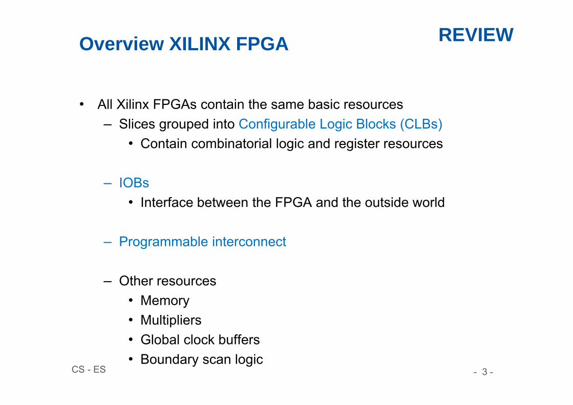
Overview XILINX FPGA
• All Xilinx FPGAs contain the same basic resources– Slices grouped into Configurable Logic Blocks (CLBs)
• Contain combinatorial logic and register resources
– IOBs• Interface between the FPGA and the outside world
– Programmable interconnect
– Other resources• Memory• Multipliers• Global clock buffers• Boundary scan logic
REVIEW

- 4 -CS - ES
Embedded Processors in FPGAs
Hard Core EP is a dedicated physical component of the chip
separate from the programmable logic E.g. Xilinx Virtex families (PowerPC 405)
Soft Core Embedded processor is also a synthesized to the FPGA to th
programmable logic on the chip E.g. Altera (NIOS), Xilinx (MicroBlaze)
REVIEW

- 5 -CS - ES
Partial Reconfiguration Technology and Benefits
Partial Reconfiguration enables: System Flexibility
• Perform more functions while maintaining communication links
Size and Cost Reduction• Time-multiplex the hardware
to require a smaller FPGA
Power Reduction• Shut down power-hungry tasks
when not needed
REVIEW

- 6 -CS - ES
Embedded System Hardware
Embedded system hardware is frequently used in a loop(“hardware in a loop“):
cyber-physical systems
REVIEW
- 7 -CS - ES
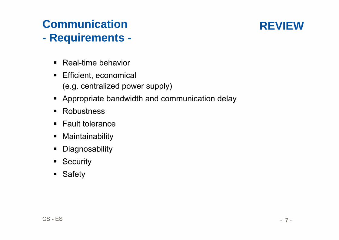
Communication- Requirements -
Real-time behavior Efficient, economical
(e.g. centralized power supply) Appropriate bandwidth and communication delay Robustness Fault tolerance Maintainability Diagnosability Security Safety
REVIEW
- 8 -CS - ES
Memory
For the memory, efficiency is again a concern: speed (latency and throughput); predictable timing energy efficiency size cost other attributes (volatile vs. persistent, etc)
REVIEW
- 9 -CS - ES
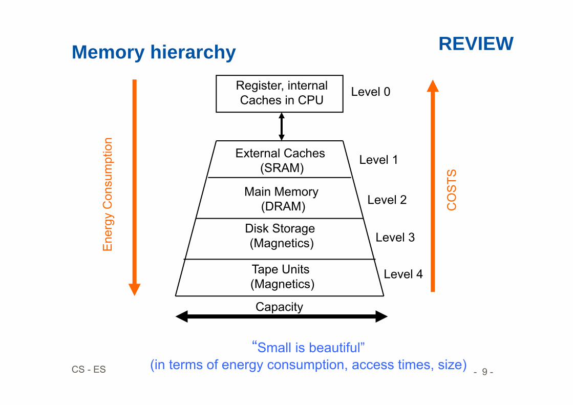
Memory hierarchyRegister, internalCaches in CPU
External Caches (SRAM)
Main Memory (DRAM)
Disk Storage (Magnetics)
Tape Units (Magnetics)
Ene
rgy
Con
sum
ptio
n
CO
STS
Level 0
Level 1
Level 2
Level 3
Level 4
Capacity
“Small is beautiful”(in terms of energy consumption, access times, size)
REVIEW
- 10 -CS - ES
REVIEW
- 11 -CS - ES
REVIEW
- 12 -CS - ES
Architecture Synthesis
HW/SW Codesign
Power Aware Computing
3.2.2011 Lecture by Bernd Finkbeiner, Head of Reactive Systems Group at Saarland University(http://react.cs.uni-sb.de/
- 13 -CS - ES
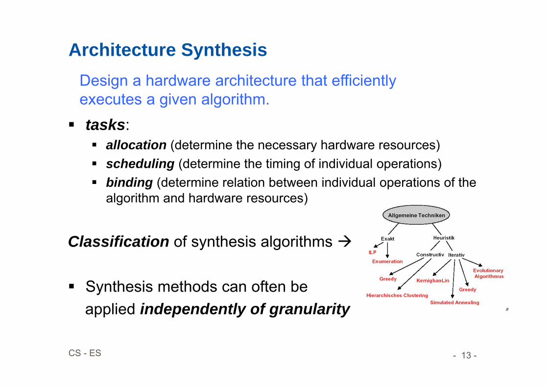
Architecture Synthesis
tasks: allocation (determine the necessary hardware resources) scheduling (determine the timing of individual operations) binding (determine relation between individual operations of the
algorithm and hardware resources)
Classification of synthesis algorithms
Synthesis methods can often be applied independently of granularity
Design a hardware architecture that efficientlyexecutes a given algorithm.

- 14 -CS - ES
Synthesis in Temporal Domain
Scheduling and binding can be done in different orders or together
Schedule: Mapping of operations to time slots (cycles) A scheduled sequencing graph is a labeled graph
[©Gupta]
+
NOP
+ <-
-NOP
1
23
4
+
NOP
+
<-
-
NOP
1
23
4
- 15 -CS - ES
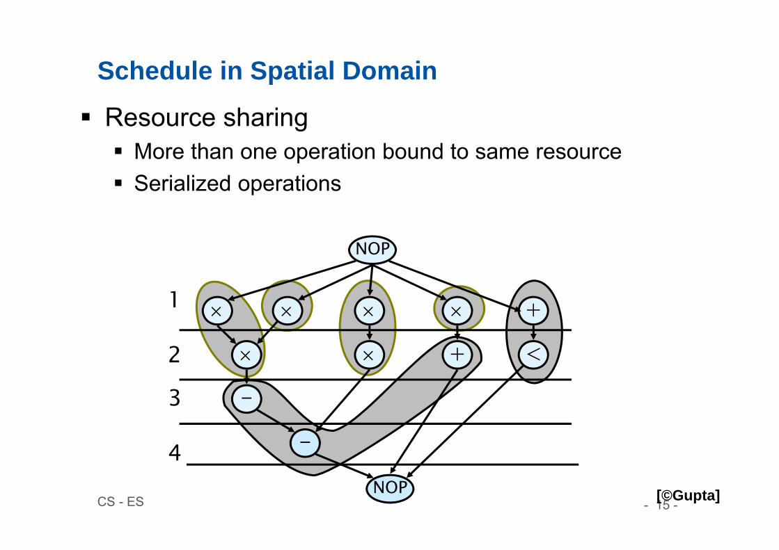
Schedule in Spatial Domain
Resource sharing More than one operation bound to same resource Serialized operations
[©Gupta]
+
NOP
+ <
-
-
NOP
1
2
3
4

- 16 -CS - ES
BASICS
Source: Teich: Dig. HW/SW Systeme;Thiele ETHZ

- 17 -CS - ES
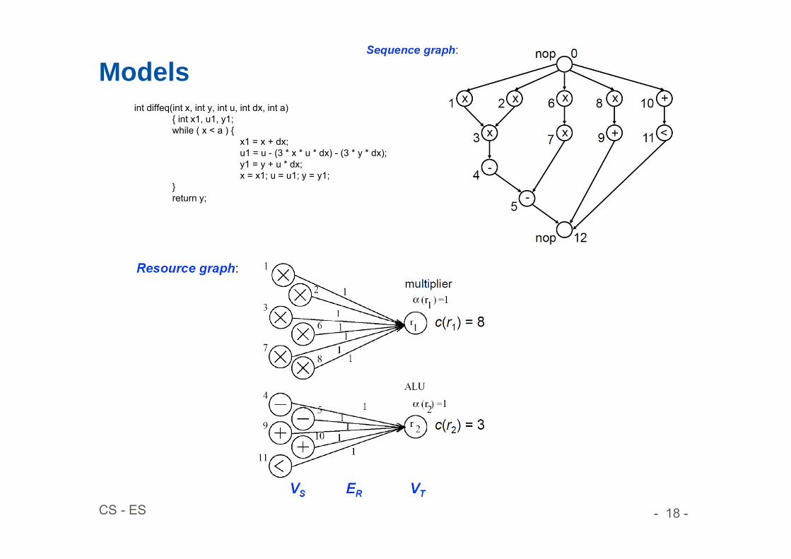
Models
- 18 -CS - ES
Modelsint diffeq(int x, int y, int u, int dx, int a)
{ int x1, u1, y1;while ( x < a ) {
x1 = x + dx;u1 = u - (3 * x * u * dx) - (3 * y * dx);y1 = y + u * dx;x = x1; u = u1; y = y1;
}return y;

- 19 -CS - ES
Allocation and Binding
- 20 -CS - ES
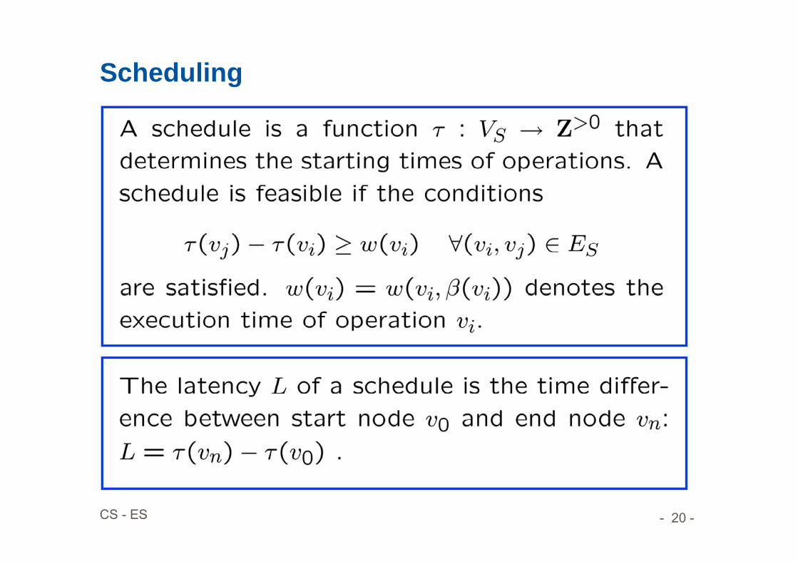
Scheduling

- 21 -CS - ES
Schedule
+
NOP
+ <-
-NOP
1
23
4
v2v1
v3
v4
v5
vn
v6
v7
v8
v9
v10
v11
L = (vn) - (v0) = 4
(v1) = (v2) … = 1
(v0) =
(v5) = 4
(vn) = 5

- 22 -CS - ES
+
NOP
+ <
-
-
NOP
1
2
3
4
Binding
Example ((r1) = 4, (r2) = 2):(v1) = r1, (v1) = 1
v2v1
v3
v4
v5
vn
v6
v7
v8
v9
v10
v11
(v2) = r2, (v2) = 1
(v3) = r1, (v3) = 2
(v6) = r1, (v3) = 3

- 23 -CS - ES
As soon as possible (ASAP) scheduling
ASAP: All tasks are scheduled as early as possible
Loop over (integer) time steps: Compute the set of unscheduled tasks for which all
predecessors have finished their computation
Schedule these tasks to start at the current time step.

- 24 -CS - ES
ASAP Schedules
+
NOP
+ <-
-NOP
1
23
4
- 25 -CS - ES
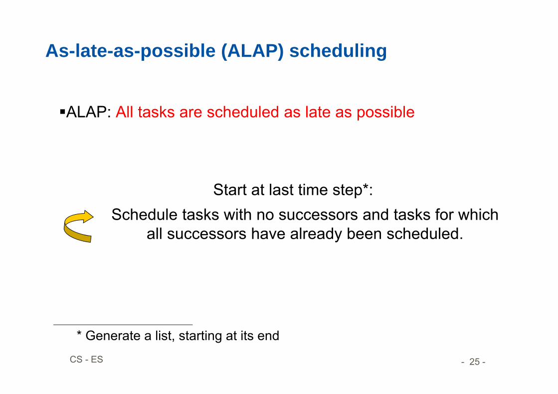
As-late-as-possible (ALAP) scheduling
ALAP: All tasks are scheduled as late as possible
Start at last time step*:Schedule tasks with no successors and tasks for which
all successors have already been scheduled.
* Generate a list, starting at its end

- 26 -CS - ES
ALAP Schedules
+
NOP
+ <-
-NOP
1
23
4

- 27 -CS - ES
Motivation Interface design. Control over operation start time.
Constraints Upper/lower bounds on start-time difference of any operation pair.
Minimum timing constraints between two operations An operation follows another by at least a number of prescribed time
steps
Maximum timing constraints between two operations An operation follows another by at most a number of prescribed time
steps
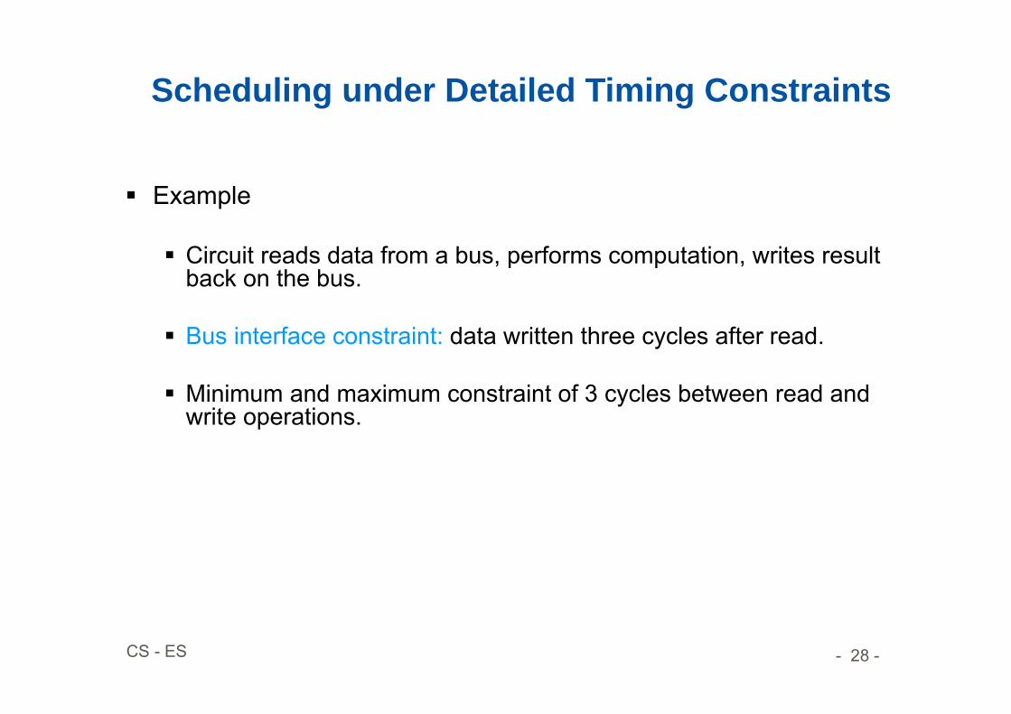
Scheduling under Detailed Timing Constraints
- 28 -CS - ES
Example
Circuit reads data from a bus, performs computation, writes result back on the bus.
Bus interface constraint: data written three cycles after read.
Minimum and maximum constraint of 3 cycles between read and write operations.
Scheduling under Detailed Timing Constraints
- 29 -CS - ES
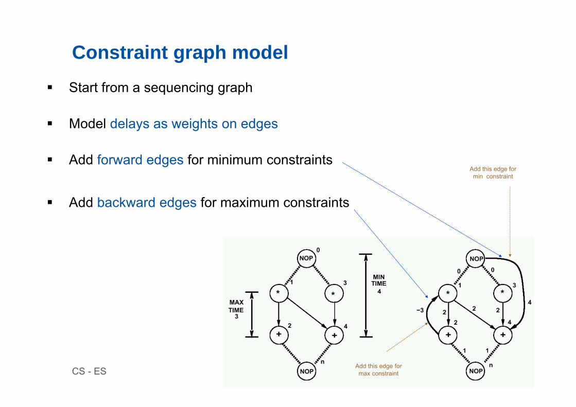
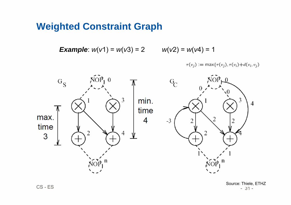
Constraint graph model Start from a sequencing graph
Model delays as weights on edges
Add forward edges for minimum constraints
Add backward edges for maximum constraints
Add this edge for max constraint
Add this edge for min constraint

- 30 -CS - ES
Weighted Constraint Graph
Source: Thiele, ETHZ
- 31 -CS - ES
Weighted Constraint Graph
Example: w(v1) = w(v3) = 2 w(v2) = w(v4) = 1
Source: Thiele, ETHZ
- 32 -CS - ES
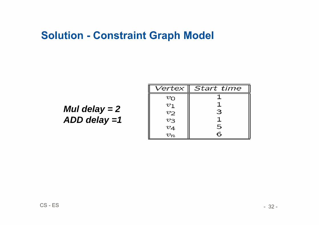
Mul delay = 2ADD delay =1

- 33 -CS - ES
(Resource constrained)List Scheduling
List scheduling: extension of ALAP/ASAP methodPreparation:
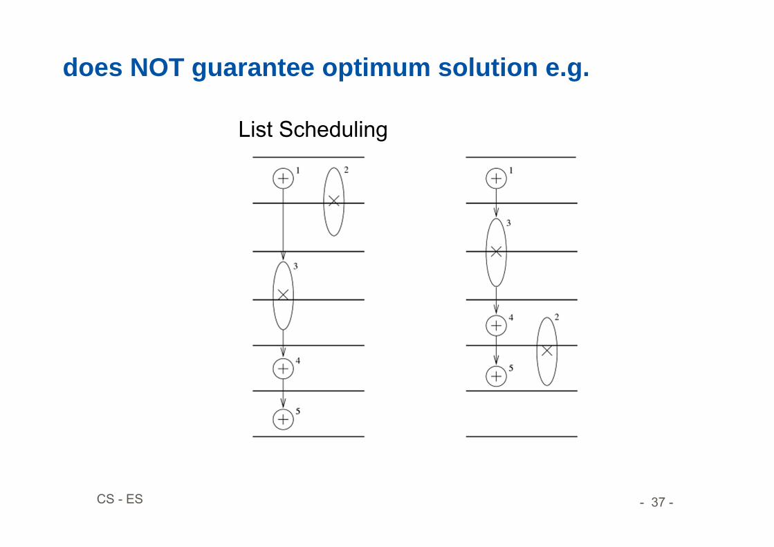
Greedy strategy (does NOT guarantee optimum solution) Topological sort of task graph G=(V,E) Computation of priority of each task:
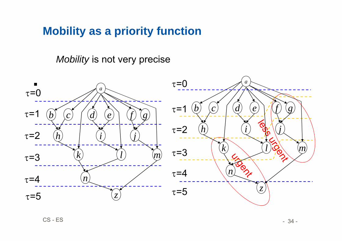
Possible priorities u:• Number of successors• Longest path• Mobility = (ALAP schedule)- (ASAP schedule)
– Defined for each operation– Zero mobility implies that an operation can be started only
at one given time step– Mobility greater than 0 measures span of time interval in
which an operation may start Slack on the start time.
Source: Teich: Dig. HW/SW Systeme
- 34 -CS - ES
Mobility as a priority function
Mobility is not very precise
=1
=2
=3
=4
=5
=1
=2
=3
=4
=5
a
b c d e f g
h i j
k l m
n
z
=0a
b c d e f g
h i j
k l m
n
z
=0

- 35 -CS - ES
Algorithm
List(G(V,E), B, u){i :=0;
repeat {Compute set of candidate tasks Ai ;Compute set of not terminated tasks Gi ;Select Si Ai of maximum priority r such that| Si | + | Gi | ≤ B (*resource constraint*)
foreach (vj Si): (vj):=i; (*set start time*)i := i +1;
}until (all nodes are scheduled);return ();
} Complexity: O(|V|)
may be repeated
for different
task/ processor classes
- 36 -CS - ES
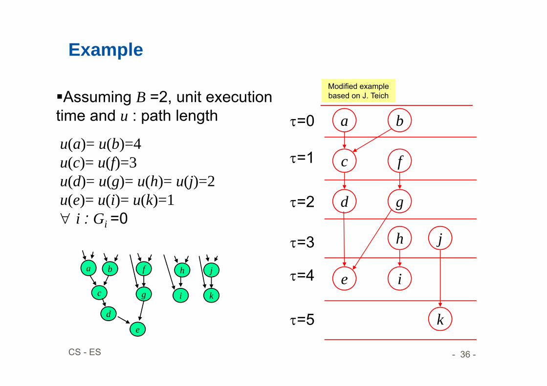
Example
Assuming B =2, unit execution time and u : path length
u(a)= u(b)=4u(c)= u(f)=3u(d)= u(g)= u(h)= u(j)=2u(e)= u(i)= u(k)=1 i : Gi =0
a b
i
c f
g
h j
k
d
ea b
c
f
g
d
e
h
i
j
k
=0
=1
=2
=3
=4
=5
Modified example based on J. Teich
- 37 -CS - ES
does NOT guarantee optimum solution e.g.
List Scheduling
- 38 -CS - ES
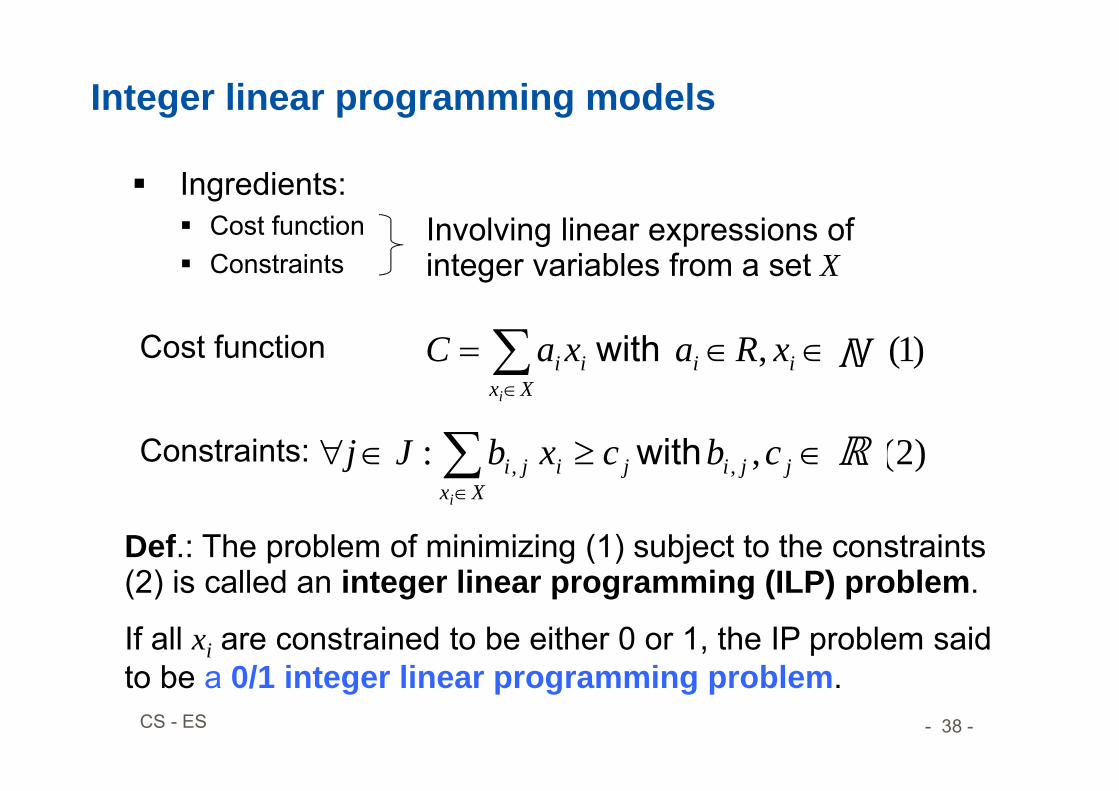
Integer linear programming models
Ingredients: Cost function Constraints
Involving linear expressions of integer variables from a set X
Def.: The problem of minimizing (1) subject to the constraints (2) is called an integer linear programming (ILP) problem.
If all xi are constrained to be either 0 or 1, the IP problem said to be a 0/1 integer linear programming problem.
Cost function )1(, NxRaxaC iXx
iiii
with
Constraints: )2(,: ,, RcbcxbJjXx
jjijijii
with
- 39 -CS - ES
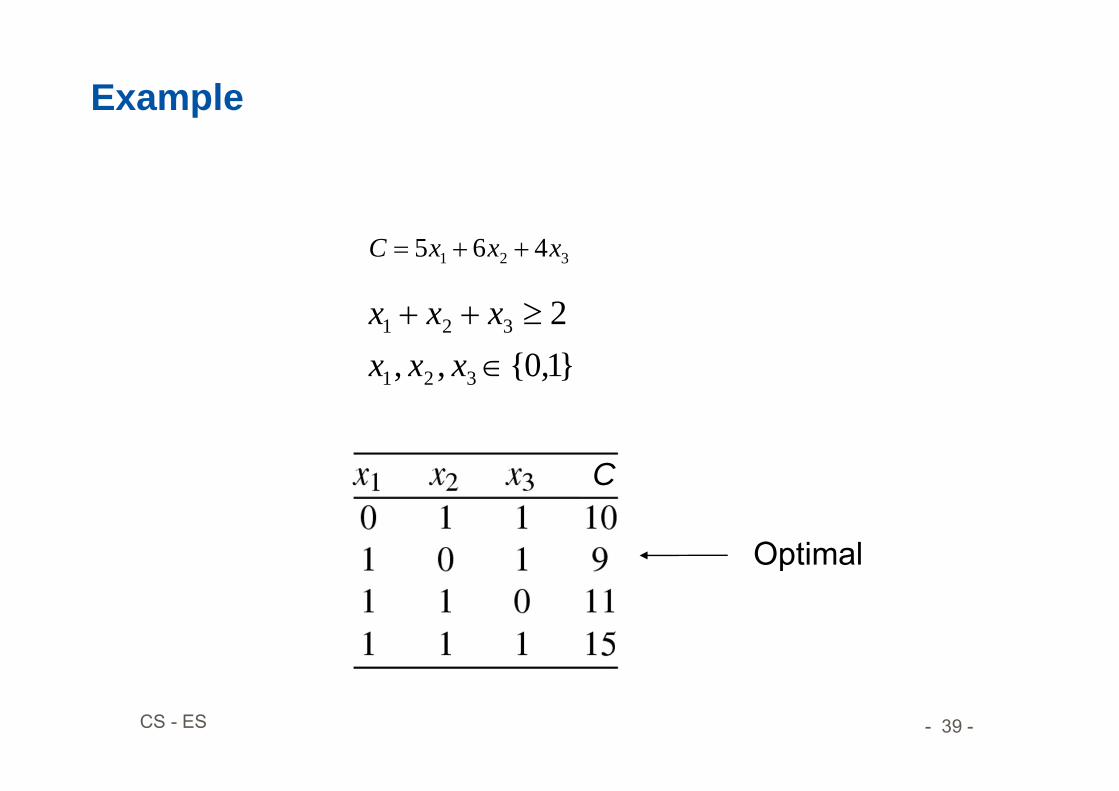
Example
321 465 xxxC
}1,0{,,2
321
321
xxxxxx
Optimal
C
- 40 -CS - ES
Remarks on integer programming
Integer programming is NP-complete
Running times depend exponentially on problem size,but problems of >1000 vars solvable with good solver (depending on the size and structure of the problem)
ILP/LP models good starting point for modeling, even if heuristics are used in the end.
Solvers: lp_solve (public), CPLEX (commercial), …

- 41 -CS - ES
Minimize latency given constraints on area orthe resources (ML-RCS)
Use binary decision variables i = 0, 1, ..., n l = 1, 2, ..., ’+1 ’ given upper-bound on latency xil = 1 if operation i starts at step l, 0 otherwise.
Set of linear inequalities (constraints),and an objective function (min latency)
ILP Formulation of ML-RCS[Mic94] p.198, Kastner, UC S. Barbara
- 42 -CS - ES
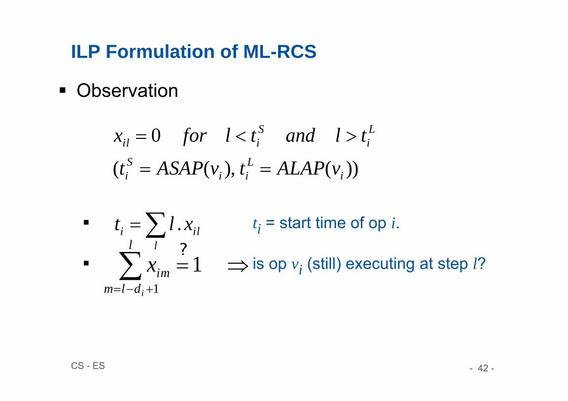
Observation
ti = start time of op i.
is op vi (still) executing at step l?
ILP Formulation of ML-RCS
))(),((
0
iLii
Si
Li
Siil
vALAPtvASAPt
tlandtlforx
ill
i xlt .
11
l
dlmim
i
x?
- 43 -CS - ES
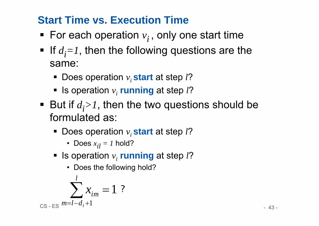
Start Time vs. Execution Time For each operation vi , only one start time If di=1, then the following questions are the
same: Does operation vi start at step l? Is operation vi running at step l?
But if di>1, then the two questions should be formulated as: Does operation vi start at step l?
• Does xil = 1 hold?
Is operation vi running at step l?• Does the following hold?
11
l
dlmim
i
x ?

- 44 -CS - ES
Operation vi Still Running at Step l ? Is v9 running at step 6? Is x9,6 + x9,5 + x9,4 = 1 ?
Note: Only one (if any) of the above three cases can happen To meet resource constraints, we have to ask the
same question for ALL steps, and ALL operations of that type
v9
456
x9,4=1
v9
456
x9,5=1
v9
456
x9,6=1

- 45 -CS - ES
Operation vi Still Running at Step l ?
Is vi running at step l ? Is xi,l + xi,l-1 + ... + xi,l-di+1 = 1 ?
vi
ll-1
l-di+1...
xi,l-di+1=1
vill-1
l-di+1
...
xi,l-1=1
vill-1
l-di+1
...
xi,l=1
. . .

- 46 -CS - ES
Constraints: Unique start times:
Sequencing (dependency) relations must be satisfied
Resource constraints
Objective: min cTt. t =start times vector, c =cost weight
ILP Formulation of ML-RCS (cont.)
l
il nix ,,1,0,1
jl
jll
ilijjji dxlxlEvvdtt ..),(
1,,1,,,1,)(: 1
lnkax reskkvTi
l
dlmim
i i
- 47 -CS - ES
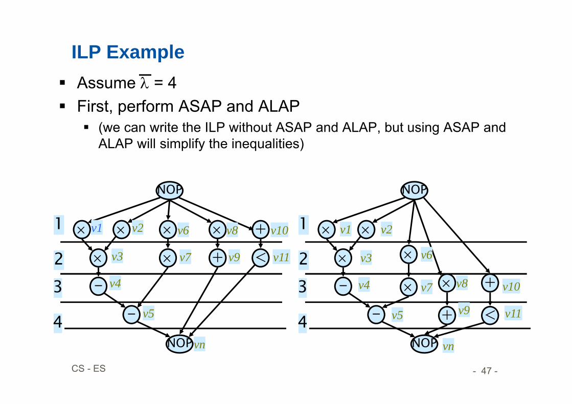
ILP Example Assume = 4 First, perform ASAP and ALAP
(we can write the ILP without ASAP and ALAP, but using ASAP and ALAP will simplify the inequalities)
+
NOP
+ <-
-NOP
1
23
4
+
NOP
+ <-
-NOP
1
23
4
v2v1
v3
v4
v5
vn
v6
v7
v8
v9
v10
v11
v2v1
v3
v4
v5
vn
v6
v7 v8
v9
v10
v11

- 48 -CS - ES
ILP Example: Unique Start Times Constraint Without using ASAP
and ALAP values: Using ASAP and
ALAP:
...1
1
4,23,22,21,2
4,13,12,11,1
xxxxxxxx
....11
11
11111
4,93,92,9
3,82,81,8
3,72,7
2,61,6
4,5
3,4
2,3
1,2
1,1
xxxxxx
xxxx
xxxxx

- 49 -CS - ES
ILP Example: Dependency Constraints Using ASAP and ALAP, the non-trivial inequalities are:
(assuming unit delay for + and *)
...01.3.2.401.3.2.4.3.201.3.2.4.3.201.2.3.2
3,72,74,5
3,102,101,104,113,112,11
3,82,81,84,93,92,9
2,61,63,72,7
xxxxxxxxxxxxxxxxxxx
- 50 -CS - ES
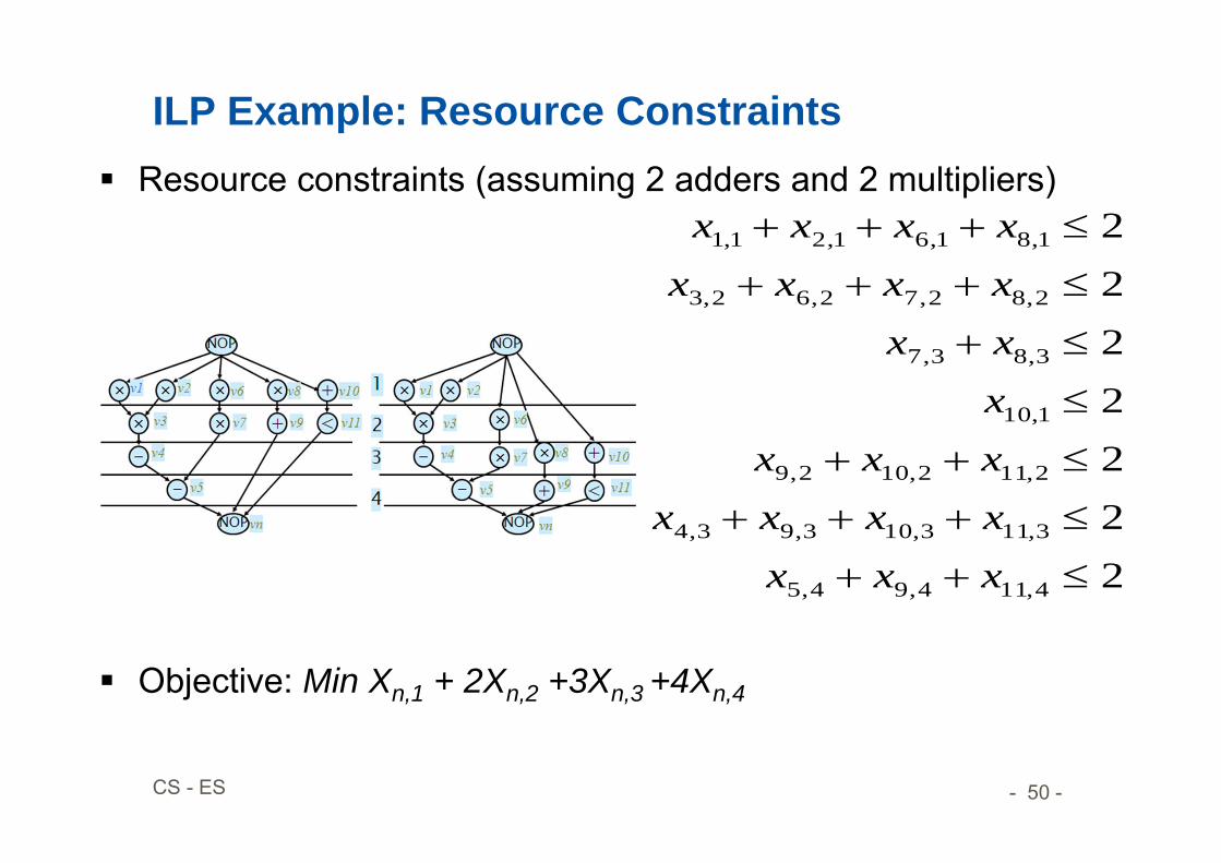
ILP Example: Resource Constraints Resource constraints (assuming 2 adders and 2 multipliers)
Objective: Min Xn,1 + 2Xn,2 +3Xn,3 +4Xn,4
2222222
4,114,94,5
3,113,103,93,4
2,112,102,9
1,10
3,83,7
2,82,72,62,3
1,81,61,21,1
xxxxxxxxxxxxxxxxxxxxx
- 51 -CS - ES
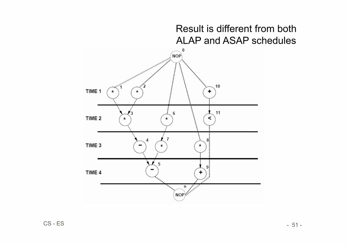
Result is different from both ALAP and ASAP schedules

- 52 -CS - ES
(Time constrained)Force-directed scheduling
Goal: balanced utilization of resourcesBased on spring modelOriginally proposed for high-level synthesisForce Used as a priority function Related to concurrency – sort operations for least
force Mechanical analogy: Force = constant x displacement
• Constant = operation-type distribution• Displacement = change in probability
* [Pierre G. Paulin, J.P. Knight, Force-directed scheduling in automatic data path synthesis, Design Automation Conference (DAC), 1987, S. 195-202]
© ACM

- 53 -CS - ES
Force-Directed Scheduling
The Force-Directed Scheduling approach reduces the amount of:
• Functional Units• Registers• Interconnect
This is achieved by balancing the concurrency of operations to ensure a high utilization of each unit.
- 54 -CS - ES
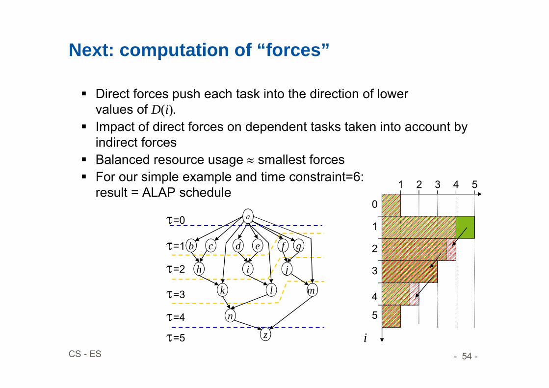
Next: computation of “forces”
Direct forces push each task into the direction of lowervalues of D(i).
Impact of direct forces on dependent tasks taken into account by indirect forces
Balanced resource usage smallest forces For our simple example and time constraint=6:
result = ALAP schedule0
1
2
3
4
5
2 31 4 5
i
=1
=2
=3
=4
=5
a
b c d e f g
h i j
k l m
n
z
=0
- 55 -CS - ES
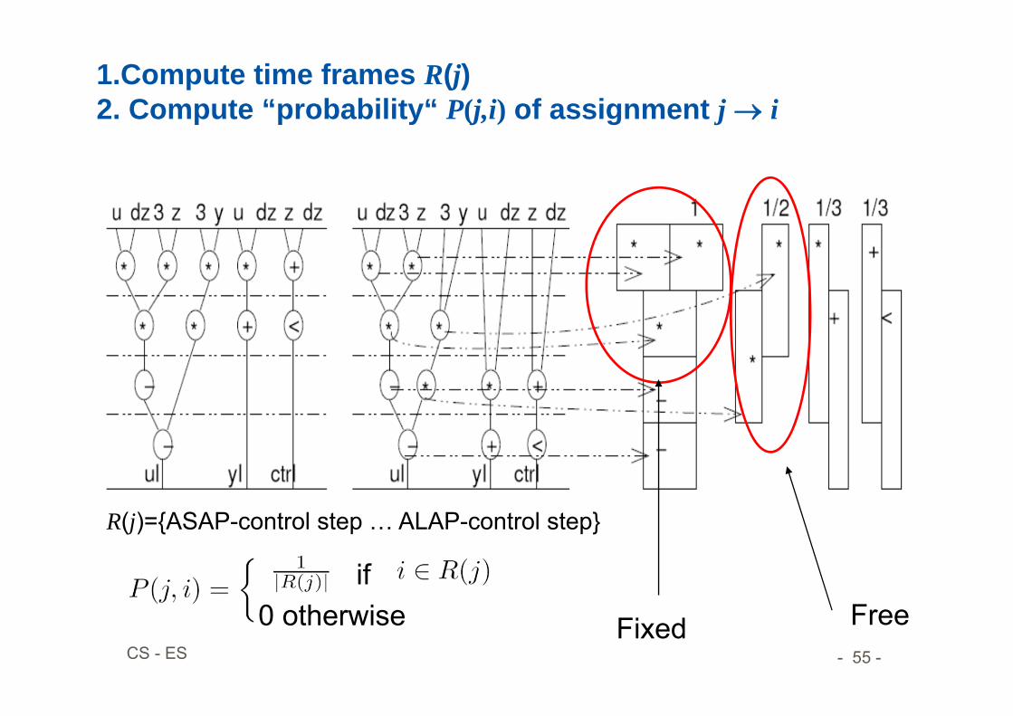
1.Compute time frames R(j)2. Compute “probability“ P(j,i) of assignment j i
R(j)={ASAP-control step … ALAP-control step}
if0 otherwise Fixed Free

- 56 -CS - ES
3. Compute “distribution” D(i)(# Operations in control step i)
P(j,i) D(i)
- 57 -CS - ES
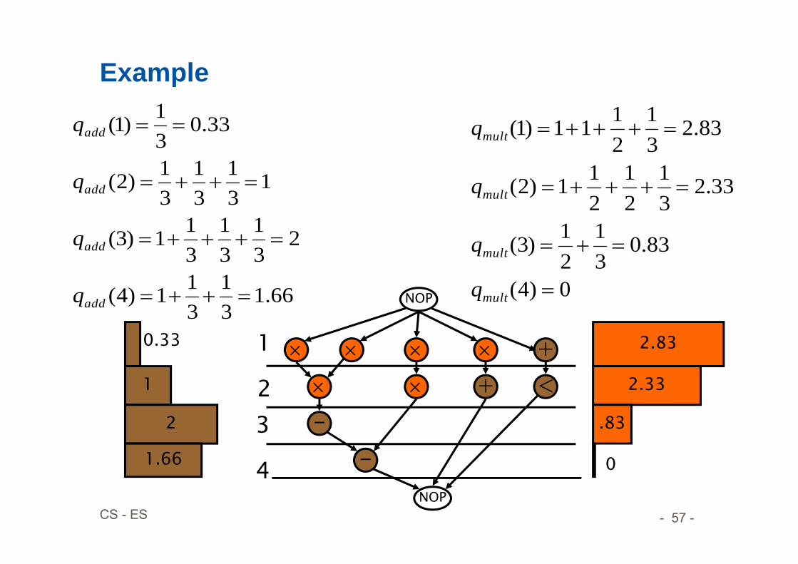
Example
+
NOP
+ <-
-NOP
1
23
4
0)4(
83.031
21)3(
33.231
21
211)2(
83.231
2111)1(
mult
mult
mult
mult
q
q
q
q
2.83
2.33
.83
66.131
311)4(
231
31
311)3(
131
31
31)2(
33.031)1(
add
add
add
add
q
q
q
q
0
1
2
1.66
0.33
- 58 -CS - ES
Scheduling – An example
b
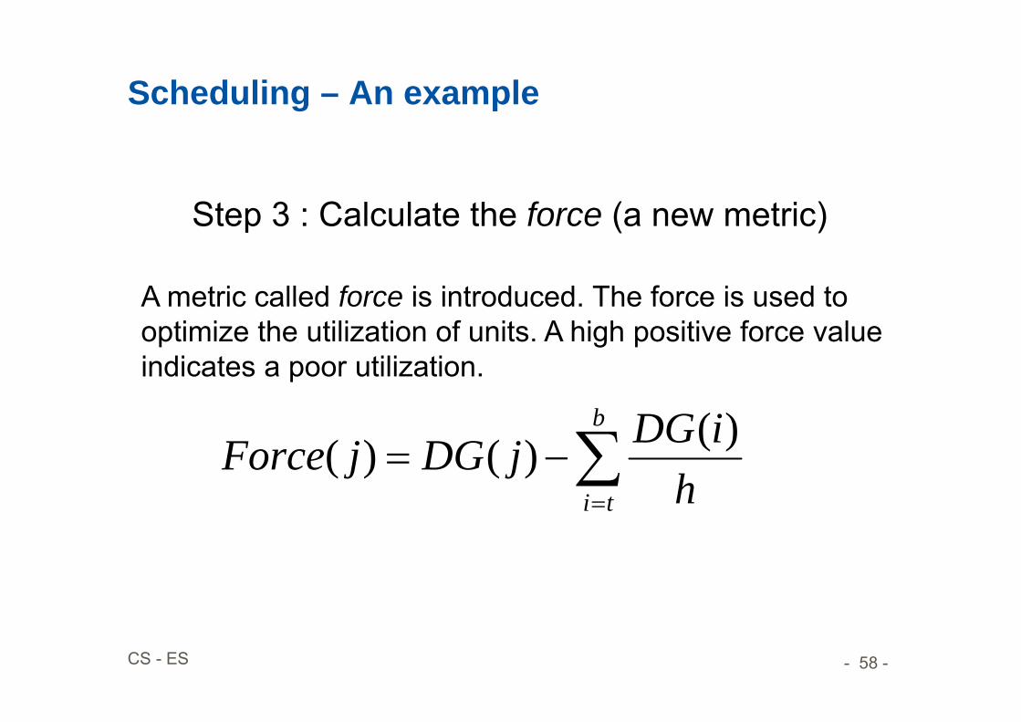
ti hiDGjDGjForce )()()(
A metric called force is introduced. The force is used to optimize the utilization of units. A high positive force value indicates a poor utilization.
Step 3 : Calculate the force (a new metric)
- 59 -CS - ES
Scheduling – An example
2
1 2)()1()1(
i
iDGDGForce
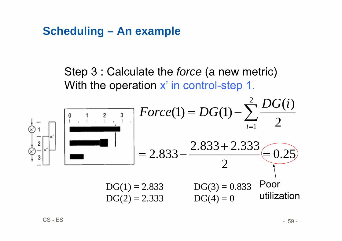
Step 3 : Calculate the force (a new metric)With the operation x’ in control-step 1.
DG(1) = 2.833 DG(3) = 0.833DG(2) = 2.333 DG(4) = 0
25.02
333.2833.2833.2
Poor utilization
- 60 -CS - ES
Scheduling – An example
3
2
2
1 2)()3(
2)()2()2(
ii
iDGDGiDGDGForce
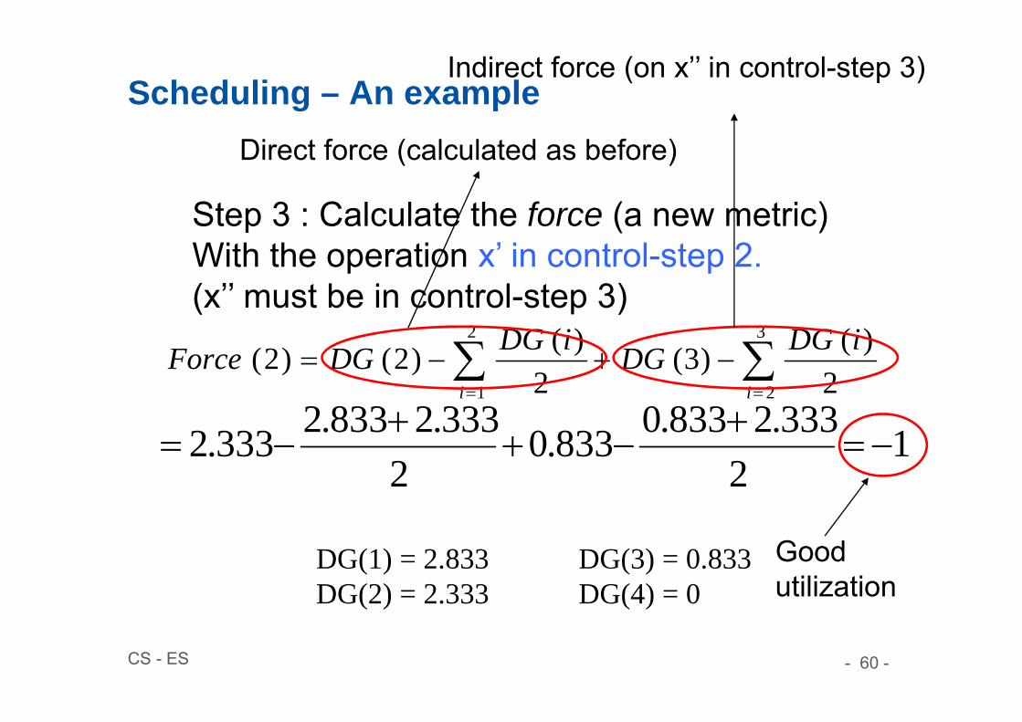
Step 3 : Calculate the force (a new metric)With the operation x’ in control-step 2. (x’’ must be in control-step 3)
DG(1) = 2.833 DG(3) = 0.833DG(2) = 2.333 DG(4) = 0
12
333.2833.0833.02
333.2833.2333.2
Good utilization
Direct force (calculated as before)
Indirect force (on x’’ in control-step 3)
- 61 -CS - ES
Scheduling – An example
By repeatedly assigning operations to various control-steps and calculating the force associated with the choice several force values will be available.
The Force-directed scheduling algorithm chooses the assignment with the lowest force value, which also balances the concurrency of operations most efficiently.
- 62 -CS - ES
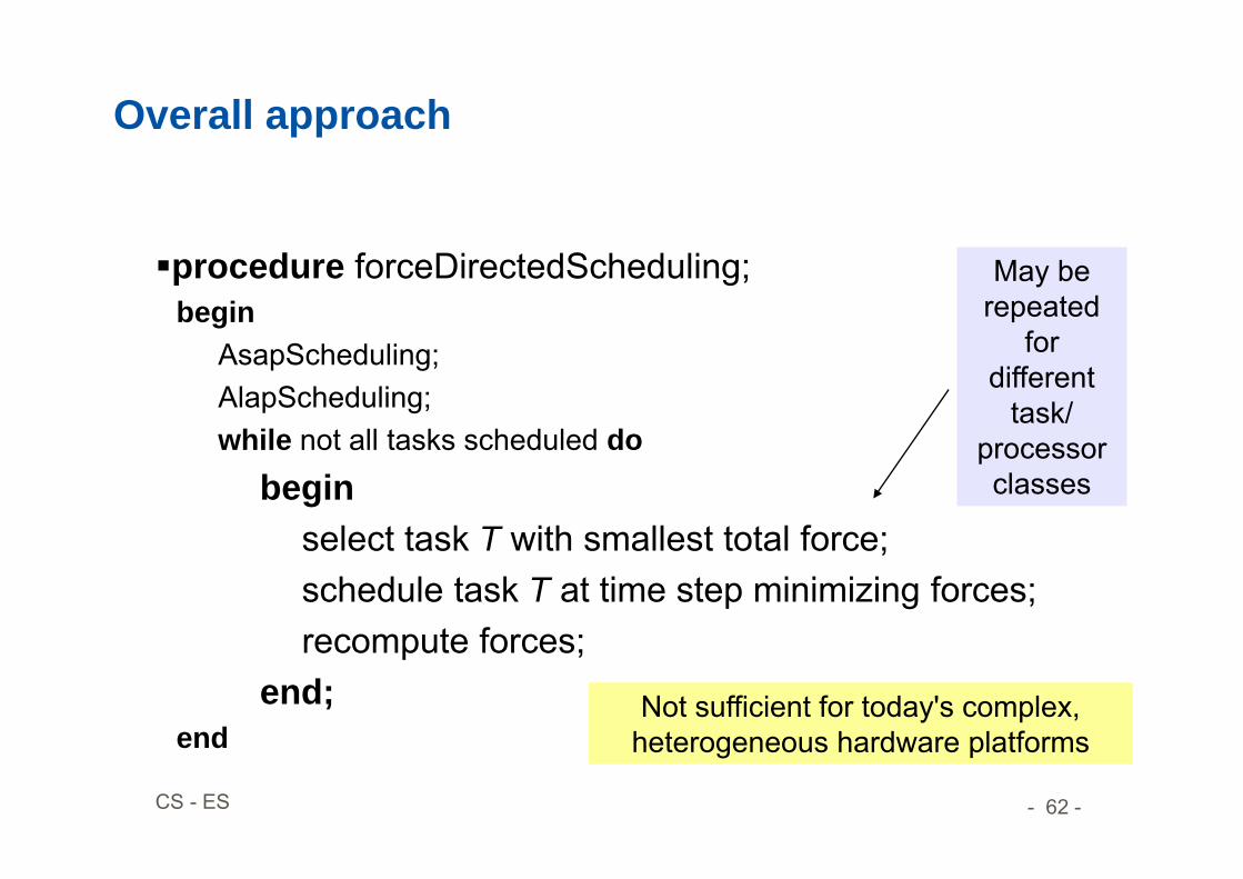
Overall approach
procedure forceDirectedScheduling;begin
AsapScheduling;AlapScheduling;while not all tasks scheduled do
beginselect task T with smallest total force;schedule task T at time step minimizing forces;recompute forces;
end;end
May be repeated
for different
task/ processor classes
Not sufficient for today's complex, heterogeneous hardware platforms
- 63 -CS - ES
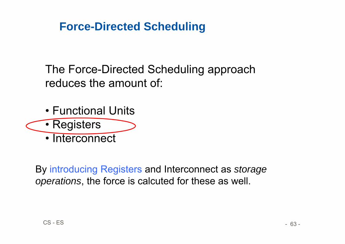
Force-Directed Scheduling
The Force-Directed Scheduling approach reduces the amount of:
• Functional Units• Registers• Interconnect
By introducing Registers and Interconnect as storage operations, the force is calcuted for these as well.

- 64 -CS - ES
Force-Directed Scheduling

- 65 -CS - ES
Architecture Synthesis
HW/SW Codesign
Power Aware Computing
3.2.2011 Lecture by Bernd Finkbeiner, Head of Reactive Systems Group at Saarland University (http://react.cs.uni-sb.de/
- 66 -CS - ES
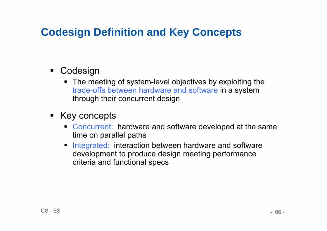
Codesign Definition and Key Concepts
Codesign The meeting of system-level objectives by exploiting the
trade-offs between hardware and software in a system through their concurrent design
Key concepts Concurrent: hardware and software developed at the same
time on parallel paths Integrated: interaction between hardware and software
development to produce design meeting performance criteria and functional specs
- 67 -CS - ES
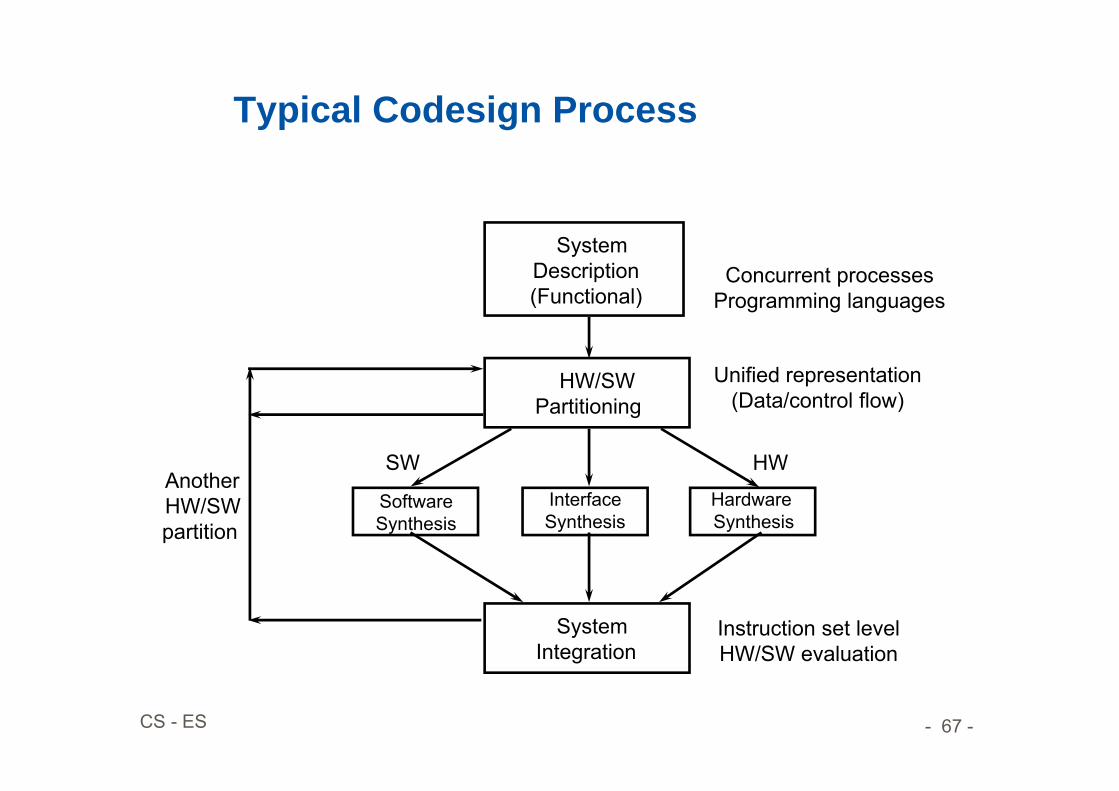
Typical Codesign Process
System Description(Functional)
HW/SWPartitioning
Software Synthesis
Interface Synthesis
Hardware Synthesis
SystemIntegration
Concurrent processesProgramming languages
Unified representation(Data/control flow)
Instruction set levelHW/SW evaluation
SW HWAnotherHW/SWpartition