
Troubleshoot your hotmail account with hotmail contact phone number

1
The impact of trade liberalization on the environment in some East Asian countries:
An empirical study
Loi Nguyen Duy, PhD candidate
CARE 2260 EMR, Faculty of Laws, Economics and Management
University of Rouen
Email: [email protected]
4.1 Abstract
We examine a cross- country data set of 6 East Asian countries1 for the period of 1980-
2006 with the aim to study the interrelationship between trade liberalization and
environmental degradation. On the basis of the parametric econometric model, we investigate
trade liberalization’s impact on the environment quality2. We take two environmental
indicators for analyses that are carbon dioxide (CO2) emissions from the consumption of energy
and primary energy consumption for analysis. The parametric model with linearity,
heteroscedasticity and autocorrelation is examined for the environmental degradation. We also
try to investigate the existence of an Environment Kuznets Curve (EKC) to describe the
interrelation between per capita income and the environment quality, and then determinants
influence the environment in the process of trade liberalization and globalization.
There is no evidence for the existence of an EKC for the relation between per capita
income and environmental indicators of carbon dioxide and energy consumption. It has an
evidence to support the pollution heaven hypothesis. This hypothesis indicates that the more
liberalization in trade would increase the level of carbon dioxide emissions and energy
consumption in these East Asian countries. There is also an evidence for the monotonically
increasing linear trend between per capita income and both pollutants. Further insightful
1 They include China, Indonesia, Malaysia, Philippines, Thailand and Vietnam
2 Environmental quality is a term of wide comprehension that relates to natural environment and built
environment, such as air and water pollution, noise, hazardous waste, solid waste, recycling, deforestation, climate
change, energy consumption, etc. In particular, air pollution consists of many pollutants, such as sulfur dioxide
(SO2), nitrogen oxides (NOx), carbon monoxide (CO), carbon dioxide (CO2), volatile organic compounds (VOCs),
chlorofluorocarbons (CFCs), ammonia NH3), etc.
2
studies on the relation between trade liberalization and environmental quality are needed in
order to make sound environmental policies for developing countries.
JEL classification: F18, Q56, C33, O11, O13
Keywords: EKC, trade liberalization, pollution, economic growth, income
4.2 Introduction
The growing literature has been investigated the relationship between economic
development and the environment quality. The relations between economic development and
the environment become more important to economic and environmental policy- making for
sustainable development. Debates have been widely taken place with regards to some
environmental problems such as the existence of an Environmental Kuznets Curve (EKC), the
pollution heaven hypothesis, the “race to the bottom” hypothesis, the factors endowment
hypothesis, etc. The EKC hypothesis, which describes a reduced form or an inverted–U shape
relationship between environmental degradation and income, indicating that the pollution level
rises as a country develops, the environment becomes cleaner on average as the economy
develops further, and increasing income passes beyond a turning point. Under the EKC
hypothesis, environmental policy plays a vital role in reducing the negative impacts of economic
activities on the environmental quality.
Since the early 1990s, many empirical studies have been examined the relationship
between income, trade liberalization and pollution in different development stages, using
cross- country and time series data. Different econometric methods have been applied to
investigate this relationship, including nonlinear and linear parametric models, semi parametric
and non parametric models, etc. However, evidences on the relationship between income,
trade liberalization and environment are mixed, particularly for developing countries. There are
quite few empirical evidences for the effects of trade liberalization on sustainable
development. The existence of an EKC depends mainly on types of pollutants, countries and
time studies, types of data - time series or cross-country data. We try to estimate and provide a

3
robust empirical evidence for the interrelations between income, trade liberalization and
environmental degradation. This study also tries to examine whether or not trade liberalization
would improve environmental quality in East Asian developing countries.
Trade liberalization is considered as removal of trade barriers3. As removal of trade
barriers could make trade grows rapidly, the environmental problems can be either alleviated
or exacerbated. It depends on the comparative advantages and efficient environmental policy.
If environmental policy is considered as an endogenous factor, then increasing liberalization
could reduce emission.
4.3 Trade liberalization and the environment: A theoretical overview
Many empirical studies have been examined the relationship between income, trade
liberalization and pollution in different development stages, using cross- country and time
series data. It possibly exist an inverted U- shaped relationship between income and pollution -
namely an EKC, which has been attracted much attention4. Some authors argued that the EKC
should be interpreted with care because of the fragile EKC and weakness of its concept (Arrow
et al., 1995, Ekins 1997, Stern and Common 2001).
The skepticisms for most empirical studies concentrate on few pollutants such as sulfur
dioxide (SO2), nitrogen oxides (NOx), carbon monoxide (CO), energy consumption, etc, and the
other pollutants have their own relations with income, not the same for all. The empirical
results can be influenced significantly by research methods, time of studies, samples, cross-
country or time series data. The impacts of economic growth on the pollutions depend on the
source of economic growth. Evidences for the impact of trade liberalization on pollution are
mixed. Antweiler et al (2001) find that trade liberalization reduces pollution. Whereas
3 Prior to trade liberalization, there are two kinds of distortions, namely trade barriers and inefficient
environmental regulations.
4 Many authors found the existence of an EKC. They are Grossman and Krueger 1993 and 1995, Shafik and
Bandyopadhyay 1992, Shafik 1994, Selden and Song 1994, Suri and Chapman 1998, Jean Agras and Nuane
Chapman 1999, and Matthew A. Cole 2004; Theophile Azomahou, Francois Laisney and Phu Nguyen Van 2006; Phu
Nguyen Van and Theophile Azomahou 2007.

4
Dasgupta et al (2002) find that trade liberalization does not affect positively on the
environment in the developing countries.
The pollution heaven hypothesis (PHH), which was supported by the studies of some
authors (Suri and Chapman 1998, Mani and Wheeler 1998). The PHH bases on the differences
in environmental stringent regulations between the North and the South5, therefore the South
has a comparative advantage in pollution intensive production while the North specializes in
clean production. The South provides pollution intensive products for the North via trade. This
is the channel that pollution transfers from the North to the South. Whereas some authors,
such as Grossman and Krueger (1993), Gale and Mendez (1998) find evidences against the PHH,
and support the factor endowment hypothesis (FEH).
The findings of evidences consistent with the PHH are quite mixed. A number of studies
investigate the environmental consequences of trade liberalization, or the impacts of income
and economic growth on the environment (Janicke et al 1997; Mani and Wheeler 1998, A. Cole
2004). However, few studies assess the net trade effects on environment or on an indicator of
sustainable development. UNEP (1999) finds evidences support trade liberalization having a
negative impact on sustainable development in several developing countries. Whereas the
UNEP’s study (2001) shows that trade has a positive effect on sustainable development in some
developing countries.
Several authors have investigated potential interactions between international trade
and the environment quality6. Trade liberalization makes countries cope with greater
competitive pressures, thus they will use resources more efficient, and as a result, pollution
emissions decrease. Trade liberalization through free trade agreements (FTA) and WTO
promote technical and environmental standards so that countries may restraint imports of
damaged environmental goods.
5 The North implies developed countries while the South refers to developing countries
6 These authors are Grossman and Krueger 1992, 1995; Shafik and Boandyopadhyay 1992; Copeland and Taylor
1994; Cole 2000 and 2004; Copeland and Taylor 2003

5
Grossman and Krueger (1995), and Copeland and Taylor (1994 and 2003) denoted three
different channels through which economic growth influences the environmental quality7 and
shapes the EKC, they are the scale effect, the composition and technique effects. The scale
effect indicates the increase of pollution resulting from economic growth and growing market
access. The composition effect implies changes in structure of an economy, as a consequence
of trade liberalization, the economy specializes growingly in activities that it has a comparative
advantage. The technique effect refers to the use of cleaner technique of production that goes
with trade liberalization. As income growth, the income- induced demand leads to cleaner
environmental regulations, higher environmental standards and environmental protection, and
access to friendly environment techniques of production. The composition effect is the channel
through which the pollution heaven hypothesis would have impacts on pollution. However, to
what extent the composition effect on pollution depends on the comparative advantages of a
country.
Most empirical studies used parametric specification such as cubic or quadratic
polynomials to examine the relations between environmental quality and per capita income,
and to test an inverted U- shape8 hypothesis of the EKC. Some studies investigated both the
inverted U- shape hypothesis and the N- shape hypothesis for developed countries9. The effect
of trade liberalization on the environment has been discussed in a number of papers10
. The
evidences are mixed, whether trade liberalization having positive or negative effects on the
7 Grossman and Krueger (1993) also decomposed the effects of trade and foreign investment liberalization on the
environment into three different channels: scale, composition and technique effects, the same the growth-
environment relation.
8 Authors such as Grossman and Krueger (1995), Shafik (1994) found evidence for the N-shape of EKC which
implies that as economic activities enlarge rapidly, the negative impact of the scale effect is always larger than the
positive impact of the other two effects- composition and technique.
9 These authors are Bruyn, Van den Bergh and Opschoor 1998; Angela Canas, Paulo Ferrao and Pedro Conceicao
2003
10 They are Suri and Chapman 1998; Antweiler et al 2001; Copeland and Taylor 2003; Cole 2004

6
environment depend on sources of comparative advantage, environmental regulations, and the
pattern of trade11
.
An empirical study applied parametric and semi parametric models to examine the
relationship between the deforestation process and per capita income, and the level of
openness. However, the study does not provide an evidence for the existence of the EKC. Trade
liberalization did not affect positively to the deforestation process (Phu Nguyen Van and
Theophile Azomahou 2007).
The pollution heaven hypothesis (PHH) states that if a country has comparative
advantages in weak environmental regulations, then the trade- composition effect will affect
negatively to the environment12
, because it will shift to the most pollution intensive production.
The PHH also indicate that poor countries may specialize in the most pollution intensive sectors
because of their comparative advantages. In other words, suppose all countries having the
similar relative factor endowment, richer countries will enforce stricter environmental
regulations that will make them specialize in clean goods.
By contrast, the factor endowments hypothesis states that the source of comparative
advantage lies in factor abundance and technology, environmental regulation does not affect or
affect little on the trade pattern. Following this view, capital abundant countries have a
comparative advantage in capital intensive production which is considered as more polluting
than labor intensive production (Mani and Wheeler 1998; Antweiler et al 2001). If this is the
case, developing countries should specialize in labor intensive sectors while developed
countries specialize in capital intensive sectors. Therefore, in practice, specialization is not
necessarily consistent with the factor abundance.
The “race to the bottom” hypothesis indicates that coping with the pressure of
international competition for foreign direct investment (FDI), countries tend to lower
environmental standards and regulations. This race would lead countries to a lowest common
11
The standard Heckscher-Ohlin model indicates that free trade makes a country with environment abundance
specialize increasingly in pollution intensive goods. However, Stolper- Samuelson theorem shows that as the price
for the use of environment is more expensive, techniques of friendly environment production can be used.
12 In this hypothesis, countries with weak environmental regulations are low-income ones.
7
environmental standard. Being affected by the international trade and competition pressures,
imports of goods from abroad, which is considered as an alternative abatement mechanism,
make pollution demand become more elastic and responsive to policy’s changes.
4.3.1 Data and Variables
4.3.1.1 Dependent environmental variables: carbon dioxide emissions from the
consumption of energy and primary energy consumption
We tested the cross- country sample of 6 countries in East Asian13
, for the period of
1980- 2006. Two distinct pollutants have been chosen as environmental variables: per capita
carbon dioxide emissions from the consumption of energy (hereafter carbon dioxide, CO2) and
per capita primary energy consumption (hereinafter energy consumption). These countries are
the newly- industrialized economies and rapid growing, consuming a large amount of energy
and generating a large amount of pollutions, including carbon dioxide and other toxic gas. We
chose these six countries in East Asian for this study because they took a large amount of
energy consumption (about 60% energy consumption by all non- OECD Asian countries, EIA
data 2008). Primary energy consumption is produced air pollutions which lead to polluting
environment, the depletion of natural resources and climate change. Moreover, energy
consumption plays an important role to keep these countries a rapid growth.
Per capita primary energy consumption is measured in quadrillion (1015
) British thermal
units (Btu), from the source of the Energy Information Administration (EIA), 2008. Per capita
primary energy consumption is considered as a pollutant. Per capita carbon dioxide emissions
from the consumption of energy are calculated in metric tons of carbon dioxide per person,
from the Energy Information Administration (EIA), 2008. Table 4.1 shows descriptive statistics
for dependent and explanatory variables.
4.3.1.2 Explanatory variables
13
They include China, Indonesia, Malaysia, Philippines, Thailand and Vietnam. Indonesia, Malaysia, Philippines,
Thailand and China are the second generation of newly industrialized economies (NIEs2). Vietnam, to some extent,
is considered as NIEs3.

8
The interactions between the quality of environment and economic variables may be
very dimensional. Many studies tried to capture these dimensions and to do comprehensive
studies on the relation between economic growth and the environment. However, due to the
lack of data on environmental pollution in developing countries, therefore this study aims at
capturing impacts of economic growth, trade liberalization and some other variables on the
environment.
4.3.1.3 Per capita GDP
Per capita GDP is measured in constant 2000 US Dollars as income measure, and the
data comes from the World Development Indicators (WDI) 2008. This variable is used to
measure interactions between incomes and pollutions. We used a quadratic functional form for
the per capita income variable because the quadratic functional form permits to check an
inverted- U shape relationship between the dependent and explanatory variables. The cubic
term, which allows us to examine the second turning point, may not be appropriated for the
newly industrialized and developing economies. Figure 4.1 presents the relation between
carbon dioxide and per capita GDP; Figure 4.4 depicts the relation between energy
consumption and per capita GDP.
Many debates on the relationship between environmental quality and per capita
income have been taken recently. The results, to some extent, aided to fill up the literature gap
concerning the role of economic and environmental policies in order to improve the quality of
life. These debates also emphasize in finding evidences for the existence of an EKC for
environmental quality. Indeed, the EKC has been found for some environmental pollutants such
as sulfur dioxide (SO2), carbon monoxide (CO), nitrogen oxides (NOx), primary energy
consumption, suspended particles, deforestation, etc.
The existence of an EKC is a necessary condition for improving environmental quality.
The important sufficient condition is to implement appropriated economic and environmental
policies for the protection of environment and sustainable development. An EKC would differ
and exist for some incomes ranges.
4.3.1.4 The growth rate of GDP
9
GDP growth rate is calculated in percentage changes and coming from the WDI 2008.
This variable is used for measuring impacts of economic growth on pollutions. The rapid growth
is necessary to improve human well-being on a sustainable basis. However, rapid growth itself
is not sufficient for the improvement of environmental quality. Environmental protection policy
and economic policies need to be coordinated for rapid growth, the improvement of well- being
and environmental quality.
4.3.1.5 Level of openness
Trade intensity or the level of openness as a percentage of GDP is measured as a share
of the sum of exports (X) and imports (M) of goods and services in GDP ((X+M)/GDP). It is
calculated on the basis of data coming from the WDI 2008. Level of openness is considered as
an indicator to measure the level of trade liberalization, trade openness and integration’s level
to the World economy. This variable aims at capturing effects of trade liberalization on the
environmental quality. Some authors14
used this indicator to estimate the impact of trade
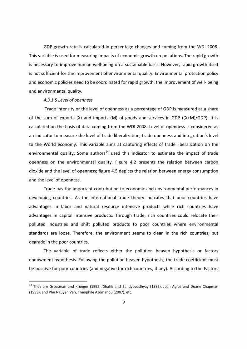
openness on the environmental quality. Figure 4.2 presents the relation between carbon
dioxide and the level of openness; figure 4.5 depicts the relation between energy consumption
and the level of openness.
Trade has the important contribution to economic and environmental performances in
developing countries. As the international trade theory indicates that poor countries have
advantages in labor and natural resource intensive products while rich countries have
advantages in capital intensive products. Through trade, rich countries could relocate their
polluted industries and shift polluted products to poor countries where environmental
standards are loose. Therefore, the environment seems to clean in the rich countries, but
degrade in the poor countries.
The variable of trade reflects either the pollution heaven hypothesis or factors
endowment hypothesis. Following the pollution heaven hypothesis, the trade coefficient must
be positive for poor countries (and negative for rich countries, if any). According to the Factors
14
They are Grossman and Krueger (1992), Shafik and Bandyopadhyay (1992), Jean Agras and Duane Chapman
(1999), and Phu Nguyen Van, Theophile Azomahou (2007), etc.

10
endowment hypothesis, if dirty industries are capital intensive and rich countries are regarded
as capital abundant, then the trade coefficient must be negative for poor countries (and
positive for rich countries, if any).
4.3.1.6 Foreign direct investment (FDI)
FDI data comes from the WDI 2008 and is measured in percentage as the total net
foreign direct investment (FDI) in current US dollars in a year divided by the GDP in current US
dollars in that same year (net FDI/ GDP). We used data on net FDI for the purpose of decrease
in autocorrelation and disturbance for this variable15
. This variable tries to estimate FDI’s
impacts on pollutions in the context of trade liberalization. Figure 4.3 depicts the relation
between carbon dioxide and foreign direct investment; figure 4.6 presents the relation
between energy consumption and foreign direct investment.
As environmental theory indicates that rich countries would shift their polluting
industries to poor countries because governments of rich countries impose stricter
environmental standards and as a result, rich countries lost the advantages in these industries.
Poor countries, which have low environmental standards, are destinations for polluted
industries from rich countries through FDI. Moreover, poor countries compete with each others
to attract FDI to meet the capital demands for economic development. The intensive
competition of FDI attraction would make poor countries lower environmental standards and
as a consequence, lead to the “race to the bottom” in environmental standards. Therefore, we
also take a test of the “race to the bottom” hypothesis.
4.3.1.7 Population density
Population density is estimated on the basis of data from the WDI 2008 and measured
in people per square kilometer. This variable is computed as the total numbers of population at
year t divided by the surface area at year t (Pop/ S). In reality, an increase in population density
would make environment degrade. The higher population density would make the environment
15
If data on accumulated FDI is made use, the probability of autocorrelation for this variable is high.

11
become more polluting. Therefore, we chose the population density as an explanatory variable
in order to measure impacts of an increase in population on pollutions.
4.3.2 Econometric model
The environmental Kuznets curves (EKC) is a “reduced- form” relationship, in which the
level of pollution is estimated as a function of per capita income. The advantage of the reduced-
form approach is that it provides the net effect of income per capita on pollution. The
econometric specification is based on the following model. Trade and FDI are included in this
EKC framework, and then the modifier model is estimated for two environmental variables.
Yit = bo + b1xit + b2xit2 + azit + μi + εit , (1)
Where y is the level of pollution being tested; x is per capita income; z is a matrix of
explanatory variables including GDP growth rate, trade intensity or level of openness, FDI, and
population density; b0 is the intercept, μi is country- specific effects and would be fixed or
random, and εit is error term. Subscripts i and t represent country and year respectively. Data
for this model is balanced cross- country panel16
.
Equation (1) allows us to test for various forms of economic and environmental
relationships. If b1 > 0 and b2 = 0, it presents a monotonically increasing linear trend, meaning
that rising income accompanies by rising level of pollution and energy consumption. If b1 < 0
and b2 = 0, it presents a monotonically decreasing linear trend, indicating the reversal
relationship between income and environmental indicators. If b1 > 0 and b2 < 0, it indicates an
EKC; If b1 > 0 and b2 > 0 present an U- shape relation that we do not expect.
Grossman and Krueger (1995) mention three different channels where economic growth
affects the environmental quality: the scale effect, the composition and technique effects. As
income grows, income elasticity toward the environment also increases. Therefore, the public
requires stricter governmental regulations and firms tend to use cleaner technique for
16
On the basis of earlier studies, aspects of a country that either do not change or change very slowly over time
are controlled for by including country specific fixed effects. Random effect is calculated for time- varying omitted
variables and stochastic shocks that are common to all countries.

12
production. Reaching a threshold income level, countries tend to give more priority for the
protection of environment.
The basic EKC models is a simple reduced-form quadratic function, recently studies
seem to deal with a cubic function17
. For having the inverted- U shape from the above
mentioned function, it needs b1 to be positive and b2 to be negative. In the standard Heckscher
- Ohlin model, the overall use of the environment does not change, and trade liberalization is
neutral for the environment.
However, Trade liberalization, association with the environmental externalities, makes
countries specialize in pollution- intensive goods in environment- abundant countries.
According to the Stolper- Samuelson theorem, the price to be paid for the use of environment
tends to increase as externalities internalized, firms adjust to less pollution- intensive
techniques for production. For the wealthier countries, 75% of all technology transfers come
from foreign trade (OECD 1995). For the developing countries, if trade liberalization raises real
income, the effects of income will reduce pollution because citizens may demand for a cleaner
environment. Thus, the technique effect would be positive for the environment.
4.3.3 The environmental Kuznets curve (EKC)
We suppose yit be the dependent pollutant variable (carbon dioxide and energy
consumption) of country i, i= 1,…,N in year t, t=1,…,T; xit is the level of real per capita GDP of
country i at year t; and zit is the matrix (p×1) vector of the other explanatory variables. Firstly,
we test the existence of an environmental Kuznets curve (EKC). Secondly, we study
determinants for pollutants through examining the functional forms and testing the statistical
hypothesis. The nonlinear and linear functional forms are checked for the purpose of finding
the most fitted functional form for the data. For simplicity, we investigate a general parametric
model below:
Yit = bo + b1xit + b2x2
it + μi + εit , (2)
17
Grossman and Krueger 1995, Shafik 1994 found evidence of an N-shape curve. This means that the negative
scale effect is bigger than the positive composition and technique effects because the economic activity enlarges.

13
Where μi, which is country- specific effects, would be fixed or random18
; εit is the error
term, and b0, b1 and b2 are parameters that are needed to be estimated.
The quadratic functional form in X is taken to test some nonlinearity in the relationship
between pollutants and per capita GDP. For the existence of an EKC, the necessary condition is
to have the nonlinear functional form for the pollutants-per capita GDP relations. The sufficient
condition is that the parameter of the equation (1): b1 > 0 and b2 < 0. If the necessary and
sufficient conditions are met, an EKC exists.
We apply the Fisher test for both pollutants: carbon dioxide and energy consumption.
For carbon dioxide, the hypothesis Ho is that the quadratic term is null, resulted in F (1, 154) =
1.99, greater than the critical value of F (0.1602), but not statistical significance at 10% level.
Therefore, we cannot reject the null hypothesis of the quadratic term. For energy consumption,
we took the same F test as for carbon dioxide, results were similar to the F test for carbon
dioxide: F (1, 154) = 1.99, higher than the critical value of F (0.1607), but not statistical
significance at the 10% level. Hence, we accept the null hypothesis of the quadratic term.
We take the test for the hypothesis of linearity in the function form, which represents
the positive results at 5% statistic significant level. For carbon dioxide, the F test for the
hypothesis that the linear term is null, resulted in F (1, 151) =887.92, far greater than the critical
value of statistic F (0.00) at the 1% significant level, thus we can reject the null hypothesis. For
energy consumption, we take the F test for the hypothesis of the null linear term, resulted in F
(1, 151) = 981.17, far greater than the critical value of F (0.00) at the 1% significant level. Hence,
we can conclude that our data for carbon dioxide and energy consumption is most fitted for the
linear functional form.
The fixed and random effect specification for carbon dioxide resulted in b1 > 0 and b2 <
0, meeting the necessary condition for the existence of an EKC. However, the data does not fit
the nonlinear functional form. The data for energy consumption does not meet the necessary
condition with the results of b1 > 0 and b2 > 0. Therefore, we can conclude that there is no
18
We estimate the fixed effect models by the fixed effect within regression and random effect by the generalized
least square (GLS) regression.

14
evidence for the existence of an EKC for pollutants of carbon dioxide and energy consumption,
and our data is most fitted the linear functional form.
4.3.4 Determinants of pollutants
As indicate above, the linear functional form is most fitted for our data, thus we have a
modified version of the equation (1)
Yit = bo + b1xit + azit + μi + εit , (3)
Where zit is a matrix (p×1) vector of the other explanatory variables, including the
growth rate of GDP, trade intensity, foreign direct investment (FDI) and population density
Firstly, We estimate the Fisher test for the null hypothesis of non significant conjoint
explanatory variables in the presence of significant conjoin explanatory variables for carbon
dioxide and energy consumption respectively, resulted in F (5, 151) = 548.32, and F (5, 151) =
699.87, far greater than the critical values of F (0.00) at 1% significant level. Thus, we reject the
null hypothesis and conclude that the explanatory variables are significant conjoint.
Secondly, we compute the F test for the null hypothesis of homogeneity in the presence
of heterogeneity. The results indicate that we can reject the null hypothesis because the
statistic F (5, 151) =284.49 for carbon dioxide and F (5, 151) = 204.93 for energy consumption,
higher than the critical values (0.00) at the 1% significant level. Thus, our data is in favor of
heterogeneous model. In other words, the fixed country effect model is preferred.
Thirdly, we compute the F test for the null hypothesis of random country effect
specification against the alternative fixed country effect specification for carbon dioxide. The
Hausman value of χ2 (4) = 14.19 is higher than the critical value of Hausman statistic test
(0.0067) at the 5% significant level. The probability of test is lower than 10% significant level.
Therefore, we can reject the null hypothesis. The fixed country effect model is preferable to the
random country effect model for carbon dioxide. Estimation for the fixed country effect for
carbon dioxide is reported in table 4.2. Estimate results indicate that per capita GDP, GDP
growth and trade are significant statistics and have significant positive impact on carbon
dioxide. However, we need to test heteroscedasticity and autocorrelation of errors before
accepting these results.

15
For energy consumption, the Hausman statistic test19
result with χ2 (4) = -33.47. This
can be interpreted as a strong evidence to indicate that we can accept the null hypothesis.
Hence, the random effect model is preferable for energy consumption. Specification for
random country effect is reported in table 4.3. Estimate results show that per capita GDP, GDP
growth and FDI are significant statistics. However, we also need to check heteroscedasticity and
autocorrelation before confirming these results.
Fourthly, we also take some necessary tests to find models that are most fitted our data.
We test the normality of residual. As presents in most econometric works, the error is supposed
to follow the law of normal distribution N (0, σ2). The results for the tests of normality in
residual are that χ2(2) = 12.37, higher than the critical value (0.0021) at the 5% significant level
for carbon dioxide and energy consumption. Thus, we can conclude that the error term follow
the law of normal distribution.
We take the test of Breusch- Pagan for the null hypothesis of homoscedasticity20
,
resulted in χ2(1) = 630.56 for carbon dioxide and χ
2(1) = 603.72 for energy consumption, both
larger than the critical value (0.00) at the 1% significant level. The Breusch- Pagan test indicates
that we can reject the null hypothesis and accept the alternative heteroscedasticity21
. It also
shows that the random effects are totally significant at the 1% significant level.
Now we take the test of autocorrelation of errors with AR (1) disturbance. The statistic
value for the F-test is that F (5, 145) = 37.60, higher than the critical value (0.00) at the 5%
significant level. Thus, we can reject the hypothesis Ho of absent autocorrelation errors for
carbon dioxide. We take a further test of Durbin- Watson for the absent autocorrelation. The
19
In case the probability of the Hausman test is greater than the critical value at the over 10% significant level. The
Hausman test cannot differentiate between the fixed effect model and the random effect model.
20 In statistic, a sequence or a vector of random variables is homoscedastic if all random variables in the sequence
or vector have the same finite variance. This is also known as homogeneity of variance. The complementary notion
is called heteroscedasticity. (Wikipedia)
21 In statistic, a sequence or a vector of random variables is heteroscedastic, if the random variables have different
variances. In contrast, a sequence of random variables is called homoscedastic if it has constant variance.
(Wikipedia)

16
observed value of Durbin- Watson = 0.46, lower than the value22
tabulated lower bound
(1.458). Hence, we can reject the null hypothesis of absent autocorrelation errors in favor of
the hypothesis positive first- order autocorrelation for carbon dioxide.
For energy consumption, the value of statistic F (5, 145) = 17.66, higher than the critical
value (0.00) at the 5% significant. The Durbin- Watson statistic value = 0.5802, lower than the
value tabulated lower bound (1.458) in the table23
at the 1% significant level. Therefore, we can
conclude that there exists the positive first- order autocorrelation for energy consumption.
In summary, we have taken the different tests for different model for determining the
best estimators and the most fitted functional form for our data. On the basis of these tests, we
can conclude that the fixed country effect model with autocorrelation and heteroscedasticity
across panels is determinant for carbon dioxide; for energy consumption, the random effect
model with autocorrelation and heteroscedasticity is determinant. We also correct the
autocorrelation of errors in these two models. In order to fit the panel data linear model with
autocorrelation and heteroscedasticity, we apply the feasible generalized least squares (FGLS)
to correct heteroscedasticity and autocorrelation structure. This method allows us to estimate
an adjust matrix of variance- covariance of errors in the presence of heteroscedasticity and
autocorrelation.
4.3.5 Empirical results
Estimation results for carbon dioxide with the correction of heteroscedasticity and
autocorrelation (table 4) indicate that the variables of per capita GDP, trade intensity and
population density are statistical significant, while the variables of GDP growth rate and FDI and
the intercept are not significant. The results imply that per capita GDP, trade and population
density have positive significant effects on carbon dioxide. The positive effect of population
density is not consistent with our arguments. The choice of population density in urban area as
an explanatory variable would be more appropriate.
22
The value in the table of Durbin- Watson is that the lower bound dL = 1.458 and the upper bound dU = 1.799
23 See 3

17
Per capita GDP and trade have significant impacts on carbon dioxide. The coefficient of
per capita GDP is greater than zero, indicating a monotonically increasing linear trend which
implies that a rise in income accompanies by an increase in the level of carbon dioxide. This
would cause concerns for the governments in developing countries for the improvement of
human well- being and the protection of environment. Thus, it needs further in- depth studies
on the income – carbon dioxide relations for making this relation more clear.
The positive trade coefficient implies the increasing linear trend between the level of
openness and carbon dioxide. This is an evidence support the pollution heaven hypothesis,
implying the poor countries are destinations for polluted industries from rich countries, and the
more liberalization in trade would make carbon dioxide increase more. Therefore, further in-
depth studies on the trade liberalization’s impacts on carbon dioxide and the role of economic
and environmental policies should be conducted.
Estimation results for energy consumption with the correction of heteroscedasticity and
autocorrelation (table 4.5) also indicate that three variables of per capita GDP, trade and
population density are statistical significant. Similar to the case of carbon dioxide, the positive
coefficient of per capita GDP supports a monotonically increasing linear trend between energy
consumption and per capita GDP. This is consistent with arguments support the linear trend for
the relation between energy consumption and per capita income (Suri and Chapman 1998). The
negative coefficient of population density is inconsistent with our arguments which state the
higher population density would make the environment more polluting.
The same as the case of carbon dioxide, the positive coefficient of trade also supports
the pollution heaven hypothesis. The evidence indicates that trade liberalization has negative
impacts on energy consumption, and an increase in the level of openness would lead to a rise in
energy consumption. There is no evidence support the factor endowment hypothesis. The
coefficients of GDP growth and FDI are insignificant and ambiguous in the regression for both
pollutants of carbon dioxide and energy consumption. Some effects may work against each
other.
Trade liberalization has resulted in increases in environmental pollutions in these
countries. Therefore, trade openness does not tend to improve environment due to the

18
efficiency use of resources and the increasing competitiveness. The use of technological
advances leading to an increase in efficiency, reduction in the cost of abatement or increases in
awareness of pollution issues raise demand for environmental regulations. In the presence of
environmental externalities, trade liberalization would harm the environmental quality and
sustainable development in these East Asian countries. Therefore, these countries should take
into account the important role of environmental policy.
4.3.6 Conclusion and policy implications
The paper provides a comprehensive picture of possible effects of trade liberalization
and per capita income on the environment quality. The evidence indicates the monotonically
increasing linear trend for the relation between per capita income and pollutants of both
carbon dioxide and energy consumption. There is no evidence for the existence of an EKC for
both environmental pollutants of carbon dioxide and energy consumption. No evidence
supports the factor endowment hypothesis (FEH) that trade liberalization is good for the
developing countries in East Asia. However, there is an evidence support the pollution heaven
hypothesis that considers the link between trade and environment. Some criteria such as
capital- labor endowment, endowment with natural resources or strictness of environment
policies could help to have better insights.
The econometric model applied in the paper can be considered as a useful tool to
examine linear, heteroscedasticity and autocorrelation data for other pollutants such as water,
industrial waste, toxic gas, etc. The application of environmental policies should be paid
attention to and consistent with specific characteristics and development stages in each
country.
There is an evidence that trade liberalization is harmful for the environment in
developing and poor countries. This indicates that economic and environmental policies need
to be coordinated to play a greater role for the reduction of negative effects of trade
liberalization on the environment.
Some global pollution issues such as CO2 and global warming require international
cooperation and need to be paid special attention to. The efforts of international cooperation

19
on the environment may avoid a “free ride problem”. The awareness and pressure of the
population could play an important role on the perceived benefits of environmental change and
a strong driving force for policy makers.
In developing countries, solving environmental problems are not necessarily hurt
economic growth (Grossman and Krueger 1995). However, developing countries always have ill
institutional capacity for making sound and strict environmental protection policies. The more
open economies to trade and foreign direct investment would increase more the pollution
levels as suggested by this study. The evidence also raises concerns for the “race to the
bottom” in developing countries because of the intensive competition of FDI attraction.
Developed countries should help developing countries to build their capacity for making sound
environmental policy, to assist techniques and finances, and to make environment friendly
methods of production.
This study may have some limitations as such the incomplete and unreliable data
availability, particularly for developing countries and the limited information gaining from the
model because of the high level of aggregation. This model would be significant increasingly if it
was broadened and included more other developing economies and explanatory variables.
Some of the empirical results are consistent with the previous studies. However, they indicate
no unique relationship between trade liberalization, per capita income and the environment for
all countries and pollutants. It needs to have further in depth- studies on the trade
liberalization’s impacts on the environment and the income- environment relations.
Having an insightful analysis for the relationship between trade liberalization and the
environment plays a crucial role and is helpful for environmental policy makers in developing
countries. At higher levels of incomes, it seems to increase demand for stricter environmental
regulations and investment in abatement technologies. It is not clear whether developing
countries follow a similar pollution- income path as some developed countries. However, there
is no doubt that income elasticity of demand for pollution intensive products falls as incomes
increase. For a late comer, Vietnam needs to build up and coordinate economic and
environmental policies for the protection of environment and achieving sustainable
development.

20

21
Table 4.1: Descriptive statistics
Variables Mean Std. Dev Min Max
Energy
consumption
26.50535 23.60734 3.08748 100.6928
Carbon
dioxide
1.778828 1.511246 0.23324 6.40294
Per capita
GDP
1216.451 1028.053 186 4535
GDP
growth rate
6.092407 4.124297 -13 15
Trade
intensity
83.16049 50.23773 19 228
Foreign
Direct Investment
(FDI)
0.024487
4
0.022366
1
-
0.0032665
0.119394
8
Populatio
n density
136.377 62.93917 41.7402
8
287.5457
Number of
countries
6
Number of
years
27
Number of
observations
162
Table 4.2: Estimation results for the fixed effect model for carbon dioxide
Variables Coefficient t- statistics

22
Intercept -0.2110687***
-1.75
Per capita GDP 0.0015687* 29.80
GDP growth rate -0.0081827***
-1.90
Trade intensity 0.0023365**
2.13
Foreign Direct Investment (FDI) 0.1688006 0.19
Population density -0.0004908 -0.42
F(5,151)1
548.32**
F(5, 151)2
284.49**
Hausman χ2 (4) test 14.19
**
Number of observations 162
Estimation is made with a cross- country sample of 6 countries in East Asia for the
period of 1980- 2006 by using the within regression. The dependent variable is the carbon
dioxide. The first F test is for the significant of conjoint explanatory variables. The second F test
is for the significant of heterogeneity. The Hausman test is for differentiating between the
random effect model and the fixed effect model. Significant level: *1%, **5% and ***10%.
Table 4.3: Estimation results for the random effect model for energy consumption
Variables Coefficient z-statistics
Intercept 2.219393* 0.92
Per capita GDP 0.0194815* 13.28
GDP growth rate 0.4979969* 3.35
Trade intensity 0.0185132 0.66
Foreign Direct Investment (FDI) 55.38848***
1.78
Population density -.0391726 -3.00
Wald chi2(5) 1563.83*
Number of observations 162

23
Estimation is made with a cross- country sample of 6 countries in East Asia for the
period of 1980- 2006 by using the Generalized Least Squares (GLS) regression. The dependent
variable is the energy consumption. Significant level: *1% and ***10%
Table 4.4: Estimation results for carbon dioxide with the correction of
heteroscedasticity and autocorrelation
Variables Coefficient z-statistics
Intercept 0.1836027 1.56
Per capita GDP 0.0012385* 18.77
GDP growth rate -0.0002581 -0.11
Trade intensity 0.0014568**
2.10
Foreign Direct Investment (FDI) 0.5181289 0.88
Population density -0.0014681**
-2.18
Wald chi2(5) 551.37*
Common AR(1) coefficient for all panels 0.8415
Number of observations 162
Estimation is made with a cross- country sample of 6 countries in East Asia for the
period of 1980- 2006 by using the feasible generalized least squares (FGLS) regression and
autocorrelation structure for correcting heteroscedasticity and autocorrelation. The dependent
variable is the carbon dioxide. Significant level: *1% and **5%
Table 4.5: Estimation results for energy consumption with the correction of
heteroscedasticity and autocorrelation
Variables Coefficient z-statistics
Intercept 0.9407799 0.61
Per capita GDP 0.0191888* 21.23
GDP growth rate -0.0036318 -0.12

24
Trade intensity 0.0261686* 3.19
Foreign Direct Investment (FDI) 5.897469 0.85
Population density -
0.0143953***
-1.67
Wald chi2(5) 678.56*
Common AR(1) coefficient for all panels 0.8475
Number of observations 162
Estimation is made with a cross- country sample of 6 countries in East Asia for the
period of 1980- 2006 by using the feasible generalized least squares (FGLS) regression and
autocorrelation structure for the correction of heteroscedasticity and autocorrelation. The
dependent variable is the carbon dioxide. Significant level: *1% and ***10%
Figure 4.1: The relationship between carbon dioxide and per capita GDP
_chn_chn_chn_chn_chn_chn_chn_chn_chn_chn_chn_chn_chn_chn_chn_chn_chn_chn_chn_chn_chn_chn
_chn
_chn
_chn_chn
_chn
_ind_ind_ind_ind_ind_ind_ind_ind_ind_ind_ind_ind_ind_ind_ind_ind_ind_ind_ind_ind_ind_ind_ind_ind_ind_ind_ind_mys_mys_mys
_mys_mys_mys
_mys_mys_mys
_mys
_mys_mys_mys
_mys_mys_mys
_mys_mys_mys_mys
_mys_mys
_mys_mys_mys_mys_mys
_phl_phl_phl_phl_phl_phl_phl_phl_phl_phl_phl_phl_phl_phl_phl_phl_phl_phl_phl_phl_phl_phl_phl_phl_phl_phl_phl_tha_tha_tha_tha_tha_tha_tha_tha_tha_tha
_tha_tha_tha
_tha_tha
_tha
_tha_tha_tha_tha
_tha_tha
_tha_tha
_tha_tha_tha
_vnm_vnm_vnm_vnm_vnm_vnm_vnm_vnm_vnm_vnm_vnm_vnm_vnm_vnm_vnm_vnm_vnm_vnm_vnm_vnm_vnm_vnm_vnm_vnm_vnm_vnm_vnm
02
46
0 1000 2000 3000 4000 5000gdppc
co2 Fitted values

25
(_chn: China; _ind: Indonesia; _mys: Malaysia; _phl: Philippines; _tha: Thailand; and
_vnm: Vietnam)
Figure 4.2: The relationship between carbon dioxide and the level of openness
_chn_chn_chn_chn_chn_chn_chn_chn_chn_chn_chn_chn_chn_chn_chn_chn_chn_chn_chn_chn_chn_chn
_chn
_chn
_chn_chn_chn
_ind_ind_ind_ind_ind_ind_ind_ind_ind_ind_ind_ind_ind_ind_ind_ind_ind_ind _ind_ind_ind_ind_ind_ind_ind_ind_ind_mys_mys_mys
_mys_mys_mys_mys
_mys_mys_mys
_mys_mys_mys_mys
_mys_mys
_mys_mys _mys_mys
_mys_mys
_mys_mys_mys_mys_mys
_phl_phl_phl_phl_phl_phl_phl_phl_phl_phl_phl_phl_phl_phl_phl_phl_phl _phl_phl_phl_phl_phl_phl_phl_phl_phl_phl_tha_tha_tha_tha_tha_tha_tha_tha_tha_tha
_tha_tha_tha_tha_tha
_tha
_tha_tha_tha_tha
_tha_tha_tha_tha
_tha_tha_tha
_vnm_vnm_vnm_vnm_vnm_vnm_vnm_vnm _vnm _vnm_vnm_vnm_vnm_vnm_vnm _vnm_vnm_vnm_vnm_vnm_vnm_vnm_vnm_vnm_vnm_vnm_vnm
02
46
0 50 100 150 200 250trade
co2 Fitted values
Figure 4.3: The relationship between carbon dioxide and foreign direct investment
_chn_chn_chn_chn_chn_chn_chn_chn_chn_chn_chn_chn _chn _chn_chn_chn_chn_chn_chn_chn_chn_chn
_chn
_chn
_chn_chn
_chn
_ind_ind_ind_ind_ind_ind_ind_ind_ind_ind_ind_ind_ind_ind_ind _ind_ind_ind_ind _ind _ind_ind_ind_ind _ind _ind_ind_mys _mys_mys
_mys_mys_mys
_mys_mys_mys
_mys
_mys_mys_mys
_mys_mys_mys
_mys_mys _mys_mys
_mys_mys
_mys_mys_mys _mys_mys
_phl _phl_phl_phl_phl_phl_phl_phl _phl_phl_phl_phl_phl _phl_phl_phl_phl_phl _phl_phl _phl_phl_phl_phl_phl _phl_phl_tha_tha_tha_tha_tha_tha_tha_tha_tha_tha
_tha_tha_tha
_tha_tha
_tha
_tha _tha_tha_tha
_tha _tha_tha
_tha_tha
_tha_tha
_vnm_vnm_vnm_vnm_vnm_vnm_vnm_vnm_vnm_vnm _vnm _vnm _vnm _vnm _vnm_vnm _vnm_vnm_vnm_vnm_vnm_vnm_vnm_vnm_vnm_vnm_vnm
02
46
0 .05 .1 .15fdi
co2 Fitted values

26
Figure 4.4: The relationship between energy consumption and per capita GDP
_chn_chn_chn_chn_chn_chn_chn_chn_chn_chn_chn_chn_chn_chn_chn_chn_chn_chn_chn_chn_chn_chn_chn
_chn
_chn_chn
_chn
_ind_ind_ind_ind_ind_ind_ind_ind_ind_ind_ind_ind_ind_ind_ind_ind_ind_ind_ind_ind_ind_ind_ind_ind_ind_ind_ind
_mys_mys_mys_mys
_mys_mys_mys_mys_mys
_mys_mys
_mys_mys
_mys
_mys_mys
_mys_mys_mys_mys
_mys_mys_mys
_mys_mys_mys_mys
_phl_phl_phl_phl_phl_phl_phl_phl_phl_phl_phl_phl_phl_phl_phl_phl_phl_phl_phl_phl_phl_phl_phl_phl_phl_phl_phl_tha_tha_tha_tha_tha_tha_tha_tha_tha
_tha_tha_tha_tha
_tha_tha
_tha_tha_tha
_tha_tha_tha_tha_tha
_tha_tha
_tha_tha
_vnm_vnm_vnm_vnm_vnm_vnm_vnm_vnm_vnm_vnm_vnm_vnm_vnm_vnm_vnm_vnm_vnm_vnm_vnm_vnm_vnm_vnm_vnm_vnm_vnm_vnm_vnm
020
4060
8010
0
0 1000 2000 3000 4000 5000gdppc
ec Fitted values
Figure 4.5: The relationship between energy consumption and the level of openness
_chn_chn_chn_chn_chn_chn_chn_chn_chn_chn_chn_chn_chn_chn_chn_chn_chn_chn_chn_chn_chn_chn_chn
_chn
_chn_chn_chn
_ind_ind_ind_ind_ind_ind_ind_ind_ind_ind_ind_ind_ind_ind_ind_ind_ind_ind _ind_ind_ind_ind_ind_ind_ind_ind_ind
_mys_mys_mys_mys_mys
_mys_mys_mys_mys_mys
_mys_mys_mys
_mys
_mys_mys
_mys_mys _mys_mys
_mys_mys_mys
_mys_mys_mys_mys
_phl_phl_phl_phl_phl_phl_phl_phl_phl_phl_phl_phl_phl_phl_phl_phl_phl _phl_phl_phl_phl_phl_phl_phl_phl_phl_phl_tha_tha_tha_tha_tha_tha_tha_tha_tha
_tha_tha_tha_tha
_tha_tha
_tha_tha_tha
_tha_tha _tha_tha_tha
_tha_tha
_tha_tha
_vnm_vnm_vnm_vnm_vnm_vnm_vnm_vnm _vnm _vnm_vnm_vnm_vnm_vnm_vnm _vnm_vnm_vnm_vnm_vnm_vnm_vnm_vnm_vnm_vnm_vnm_vnm
020
4060
8010
0
0 50 100 150 200 250trade
ec Fitted values

27
Figure 4.6: The relationship between energy consumption and foreign direct
investment
_chn_chn_chn_chn_chn_chn_chn_chn_chn_chn_chn_chn _chn _chn_chn_chn_chn_chn_chn_chn_chn_chn_chn
_chn
_chn_chn
_chn
_ind_ind_ind_ind_ind_ind_ind_ind_ind_ind_ind_ind_ind_ind_ind _ind_ind_ind_ind _ind _ind_ind_ind_ind _ind _ind_ind
_mys _mys_mys_mys
_mys_mys_mys_mys_mys
_mys_mys
_mys_mys
_mys
_mys_mys
_mys_mys _mys_mys
_mys_mys_mys
_mys_mys _mys_mys
_phl _phl_phl_phl_phl_phl_phl_phl _phl_phl_phl_phl_phl _phl_phl_phl_phl_phl _phl_phl _phl_phl_phl_phl_phl _phl_phl_tha_tha_tha_tha_tha_tha_tha_tha _tha
_tha_tha_tha_tha
_tha_tha
_tha_tha _tha
_tha_tha_tha _tha_tha
_tha_tha
_tha_tha
_vnm_vnm_vnm_vnm_vnm_vnm_vnm_vnm_vnm_vnm _vnm _vnm _vnm _vnm _vnm_vnm _vnm_vnm_vnm_vnm_vnm_vnm_vnm_vnm_vnm_vnm_vnm
020
4060
8010
0
0 .05 .1 .15fdi
ec Fitted values
References
Angela Canas, Paulo Ferrao and Pedro Conceicao (2003). A new environmental
Kuznets curve? Relationship between direct material input and income per capita: evidence
from industrialized countries. Ecological Economics 46 (2003) p217- 229
Antweiler, Werner, Brian R. Copland, and M. Scott Taylor (2001). Is free trade good for
the Environment? American Economic Review 91 (4) pp 877- 908
Bandyopadhyay, subhayu, and Nemat Shafik (1992). Economic growth and
environmental quality: time- series and cross- country evidence. Background paper for the
World Development Report 1992, World Bank, Washington
Bruyn, Van Den Bergh and Opschoor (1998). Economic growth and emission:
reconsidering the empirical basis of environmental Kuznets curve. Ecological Economics 25
(1998), p161- 175
Cole, M.A., (2000). Air pollution and “dirty” industries: how and why does the
composition of manufacturing output change with economic development? Environmental and
resource Economics 17(1) 109- 123

28
Cole, Mathew A. (2004). Trade, the pollution heaven hypothesis and the environmental
Kuznets curve: examining the linkages. Ecological Economics 48, pp. 71- 81
Cole, Mathew A. (2003). Development, trade and the environment: how robust is the
environment Kuznets curve? Environment and development economics, 8, pp.557-580,
Cambridge
Cole, M.A, Eliliot, R.J.R., (2003). Determining the trade- environment composition effect:
the role of capital, labor and environmental regulations. Journal of Environmental Economics
and Management 46(3), pp. 363- 83
Cole, M.A., Rayner, A.J., Bates, J.M., (1997). The environmental Kuznets curve: an
empirical analysis. Environment and development economics 2(4), pp. 401- 16
Copland, Brian R., and M. Scott Taylor (2004). Trade, growth and the environment.
Journal of Economic Literature, 42(1), p7-71
Copeland, Brian R., and M. Scott Taylor (1995). Trade and transboundary pollution.
American Economic Review, 85, pp.716- 37
David Stern (2004). The rise and fall of the environmental Kuznets curve. World
development Vol. 32, No8, 2004, p1419- 1439
Grossman, Gene M., and alan B. Krueger (1995). Economic growth and the
environment. Quarterly Journal of economics, 110(2) pp. 353-77
Jean Agras and Duane Chapman (1999). A dynamic approach to the environmental
Kuznets curve hypothesis. Ecological Economics 28 (1999), p267- 277
Mariano Torras, James K. Boyce (1998). Income, Inequality, and pollution: a
reassessment of the environmental Kuznets Curve. Ecological Economics 25, pp.147- 60
Marzio Galeotti, Alessandro Lanza and Francesco Pauli (2006). Reassessing
environmental Kuznets curve for CO2 emissions: A robustness exercise. Ecological Economics
57 (2006) p152- 163
Matthew Clarke and Sardar Islam (2005). Diminishing and negative welfare returns of
economic growth: an index of sustainable economic welfare for Thailand. Ecological Economics
54 (2005), p81-93
Neha Khanna and Florenz Plassmann (2004). The demand for environmental quality
and the environmental Kuznets curve hypothesis. Ecological Economics 51 (2004), p225- 236
Phu Nguyen Van and Theophile Azomahou (2007). Nonlinearities and heterogeneity in
environmental quality: An empirical analysis of deforestation. Journal of Development
Economics 84 (2007), p291- 309

29
Robert Kaufmann, Brynhildur Davidsdottir, Sophie Garnham and Peter Pauly (1998).
The determinants of atmospheric SO2 concentrations: reconsidering the environmental Kuznets
curve. Ecological Economics 25 (1998), p209- 220
Soumyananda Dinda (2005). A theoretical basis for environmental Kuznets curve.
Ecological Economics 53 (2005), p403-413
Stern, DavidI., and Michael S. Common (2001). Is there an Environmental Kuznets
curve for sulfur? Journal of Environmental Economics and Management, 41(2), pp. 162-78
Theophile Azomahou, Francois Laisney and Phu Nguyen Van (2006). Economic
development and co2 emissions: a nonparametric model approach. Journal of Public
Economics 90 (2006), p1347- 1363
World Bank (2008). World Development Indicators 2008, World bank Washington
World Bank (2001). Is globalization causing a “race to the bottom” in environmental
standards? World Bank Briefing Paper, part four: Assessing Globalization, Economic policy
group and development economic group, World Bank, Washington.
www.eia.doe.gov/
www.ddp-ext.worldbank.org/ext/DDPQQ
www.earthtrends.wri.org, etc