AAMRL-TR-87-O11

OTiC FILE ctWy

eM HUMAN JOINT ARTI.CULATION ANDCO MOTION-RESISTIVE PROPERTIES

S AUI E. ENGINsI:UENN-MUH CHEN

THE OHIO STATE UNIVERSITYDEPARTMENT OF ENGINEERING MfECHANICS1314 KINNEAR ROADCOLUMBUS, 01143212

JANUARY1987

FINAL REPORT FOR PERIOD SEPTEMBER 1983 - JULY 1986RF PROJECT 763802/715689CONTRACTNO. F3361S-83-C-0510

Approved for public release; distribution is unlimnited.

HARRY G. ARMSTRONG AEROSPACE MEDICAL RESEARCH LABORATORY

HUMAN SYSTEMS DIVISION

WRIGHT-PATTERSON AIR FORCE, BASE, OHIO 45433-65 73 F

A ~ ~ M~' 87

! t )N.....-....

NOTICES

When US Government drawings, specifications, or other data are used for any purpose other than adefinitely related Government procurement operation, the Government thereby incurs no responsibilitynor any obligation whatsoever, and the fact that the Government may have formulated, furnished, orin any way supplied the said drawings, specifications, or other data, is not to be regarded byimplication or otherwise, as in any manner licensing the holder or any other person or corporation, orconveying any rights or permission to manufacture, use, or sell any patented invention that may in anyway be related thereto.

Please do not request copies of this report from the Armstrong Aerospace MedicalResearch Laboratory. Additional copies may bu purchased from:

National Technical Information Service5285 Port Royal Road"Springfield, Virginia 22161

Federal Government agencies and their contractors registered with Defense Technical InformationCenter should direct reqaests for copies of this report to:

Defense Technical Information CenterCameron StationAlexandria, Virginia 22314

TECHNICAL REVIEW AND APPROVAL

AAMRL-TR-87-011

The voluntary informed consent of the subjects used in this research was obtained as required by AirForce Regulation 169-3.

This report has been reviewed by the Office of Public Affairs (PA) and is releasabje to the NationalTechnical Information Service (NTIS). At NTIS, it will be available to the general public, includingforeign nations.

This technical report has been reviewed and is approved for publication.

FOR THE COMMANDER

HENNIN VON GIERKE, Dr IngDirectorBiodynamics and Bioengineering Division

Armstrong Aerospace Medical Research Laboratory

REPORT DOCUMENTATION PAGEis. flEPOil SECURITY CLASSIFICATION llb RISRICIV* MAKI

Unc~lauuif ied1e.SCVRI TY C%.ASS.IPICATION AUTHORITY 3. O!STRI BUTIONIAVAI LAS ILITY OF REPORT

Approved for public relesuel distributionDw ECLASIFICAIý01OIOWNt4CRAINOSCH4iaULE9 is unlimuited.,

4. praFORMING ORGANIZIATION REPORT NUMBER(S) &. MONITORING ORGANIZATION REPORT NUMBERtS)

"61NAMIE 01: PE AFORMING ORGANIZATION b. OFFICIE SYMBOL 7&. NAME OF MONITORING ORU3ANIZATIONTh %hi 1U State Univrersity OrSD, APSC.

______________________ _____________ AAI4RL/BBM

ScA0~iS~4F. si.ato l~ew 7b. A0011123 tflty. State mod 9110Code)1114 Kion-i~r Road

CoumusOil 43212 Wright-Patterson AFB OHt 45433-6~573

Sm. NAME OF FUNDINGIMP.ONSORING Sb., oprFIC SYM80L 9. PROCUREMENT INSTRUMENT IDENTIFICATION NUMBeftORGANIZAT ION Ieplebi

AAJ4RL BBM F33615-.83-C-0510We, ADDAVIS fitei,. Steh# spýd rip Coko.i .14 SOURCE *P FUNDING NOS. ___________

PROGRAM PROJECT TASK WORK UNIT

Wright-, -tte rson APB OH 45433-6573 ELK ME NT NO. NO. NO. NO.

ArticUlation A Motion-Resistive Properties______Ij01V2.PERS0NAL AUTt46R.iS

Engift:, 'Al E. i.-ind Chen, Shuenn-tMuh*13s. TYPE OF NEPORT ~131k TIME COVERED 114. OATS OF REPORT (Yr.,. Mo.. Day; 15. PAGE COUNT

C Final IFRO UB L T0O3JUJUI April. 1987 I 189it. SIPPLeMENTARiYNOTJATION

I?. COSATI Oca s Is. SUBJECT TERMS eWantinue Got ,ewrse it nescwery end identify by block number)a .GRoUP sue. to Biomechanics, elbow complex, joint kinematics, joint sinus,

joint restoring forces, joint passive forces, hip complex,shoulder cornplex, sonic digitizer, statistical data base.41

As. ABSTRACT i~ue'tnhe. an reue'rit, if necessary and identify by Maock number)

Three-dimensional joint kinematics and motion resistive properties were measuredfor tUse shioulder, hip and elbow joints on ten male volunteers. A sonic three-I1imensional spatial digititting system was used to track multiple targets on adjacertbody segmetILS while each of the segments was moved through a maximum voluntary rang~eOr motion and also while it was subsequently forced to maximum voluntarily allowableratnqs by anI external force applicator. The target data were used to reconstruct thesetiniviA kinematics, which were then related to the force required to attain a givenjoint orientation. 'rhe final data are provided, in a qIlobographic presentation inwhich equal force. viilues are depicted, as contours on a global surface. The resistive

* Ior&o40.4I' ýie xpressed as function-s oif the orien-tation angles in spherical harmoni

ý6(ontinued on reverse)

213 DIST RI RUTIONIAVAILASOLITY OF ABSTA~cr 21. ABSTRACT SECURITY CLASSIFICATION

utJNCt.A:,SIFkEC),UN1 IM11kU SAMIE AS NFT. F) OfiC USERS 0 unclassified

220. NAML OF H IW-NSIHlIL INn, ViDUAL 22b.. TELEPHONE NUMBER 122c. OFFICE SYMBOL(include Arve Code)

.INTS KAI4EPS 513/255-3608 AAMRL/8BB4

OD FORM 1473, 83 APR EDITION OF I JAN 73 IsoBSOLETE._____SECURITY CLASSIFICATION OF THIS PAGE

OMP'ITY CLAhSIFICATION OP THIS PAGE

Sexpansion form. Statistical analyses have been performed on these data to generate

Block 19 (Abstract) tinued.

both means and variances for the kinematics and resistive force properties. The datd

have direct applicability to better understanding of the kinematics of human long bonejoint.l providing preliminary limits for safe joint ranges of motions and forces;and serving as a data base for analytical and mechanical models of the human body

8iCUmrTY CLARRIFIrATION OiF T"Ig Pl•MP

PREFACE

The research work described in this report was performed for theModeling and Analysis Branch of the Armstrong Aerospace Medical ResearchLaboratory at Wright-Patterson Air Force Base under Contract No.F33615-83-C-0510. The research was monitored by Dr. Ints Kaleps, Chief ofthe Modeling and Analysis Branch, and it was administered by The Ohio StateUniversity Research Foundation under Project No. 715689.

The authors also acknowledge the utilization of some of the hardwareand software, developed by one of the former graduate students of thesenior author, namely, Dr. Richard D. Peindl, in various aspects of ther.•search work prestnted in this report.

j WAS

'-~~ -~, .'-~-~- .--. ~-~ ~&~ 1.~ A.f-%A.~31 MR . A 3 A LAM MA-,l at -I~ W, 26n UILA ALA&F XA &JUtAUO&fl Angl

TABLE or CO0TRMt8

PAGE

LIST OF FIGURES . . . . . . . . . . . . . . . . . . . . . ..... iv

LIST Or TABLES . . ......................... viii

1. INTRODUCTION . .. .. . .. 1

1.1 Background . . i . . . . . . . . 11.2 Definitions of Joinj Sinus and* lo•bograhic Representation 31.3 Scope of Research . . . . . . . . .0. . . . . . . . . . . 4

2. KINEMATICS BY MNS OF AN OVURDETRKI4NATE NUMBER OFSONIC MIUTTERS. . . 62.1 Review of the Sonic*Digitizingo Tc~hn~ique - . . *- *- *- *- *- *- 62.2 moving Rigid-Body Kinematics and Initialization of a

Baseline Data Set . .-. . . . . . . . . . .b. . . . . . . 82.3 Selection of the *Most Accurate" Axis System on the

moving Body. . . . . . . . . . . . . . .. . . . . . . ... 11

3. BIOMECHANICAL PROPERTIES OF THE HUMAN SHOULDER COMPLEX. . . . . 153.1 Introduction . . . . . . 1. 5 . . 0 . . a * . * . a 0 a i13.2 Determination of the Maximum Voluntary Shoulder

Complex Sinus . . . . . . . . * 0 0 . . 0 0 * * * * . 0 * 153.3 Passive Resistive Properties Beyond the Shoulder

Complex Sinus. .0. . . . a ..0. . . . . . . . .. ... .. 203.4 Statistical Analysis . . . . . . . . . . . . . . . . . a a 263.5 Coordinate Transformations Among the Fixed Body,

Individual Joint and Mean Joint Axis System . . . . . . . 323.6 Statistical Data Base for the Biomechanical

Properties of the Human Shoulder Complex . . . . . . . . . 35

4. BIONECHANICAL PROPERTIES OF THE HLAN HIP COMPLEX . . ..... 564.1 Introduction . . . . . ...................... 564.2 Determination of the Hip Complex Sinus . . . . * . 574.3 Determination of the Passive Resistive Properties . ... 604.4 Statistical Data Base for the Biomechanical

Properties of the Human Hip Complex. . . . . . . . 70

5. BiOMECHANICAL PROPERTIES OF THE HUMAN HUMERO-ELBOW COMPLEX... 835.1 Introduction . . . . . . . . . . . . . . . .. ... . 835.2 Determination of the Humero-elbow Complex Sinus. . . . . . 835.3 Determination of the Passive Resistive Properties

Beyond the Full Elbow Extension .............. 885.4 Statistical Data Base for the Biomechanical

Properties of the Human Humero-Elbow Complex . . . . . . . 93

6. CONCLUDING REMARKS. . . . . . . . . . . . . ........ . . . 103

APPENDIX A: SELECTED ANTHROPOMETRIC MF.JSUREMENTS OF TEN SUBJECTS . . 104

APPENDIX B: COMPUTER PROGRAMS FOR DATA ACQUISITION AND ANALYSIS. .-. 105

REF3REkNCES . . . . . . . . . . . .. . .. ... .. . . * . . . . . . 173

iii

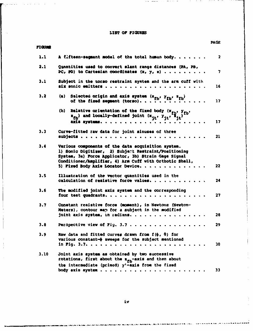
LIST OF FIGURES

PAGEFIGUR

1.1 A flfteen-segmwnt model of the total human body. . . . . . . 2

2.1 Quantities used to convert slant range distances (PA, Po,PC. PO) to Cartesian coordinates (x, y, z) . . . . . . 7

3.1 Subject in the torso restraint system and the arm cuff withsix sonic eitters ...................... 16

3.2 (a) Selected origin and axis system (xfb, Yfb' *fb)of the fixed segment (torso) .............. 17

(b) Relative orientation of the fixed body (xfv , yfbafb) and locally-dofined joint (xit* yjt -jt)axis systems . . . . . . . . . . . . . . . . . . . . . 17

3.3 Curve-fitted raw data for joint sinuses of threesubjects . . . . . . ... . .....0 0000........0. 21

3.4 Various components of the data acquisition system.1) Sonic Digitizer# 2) Subje.t Restraint/PositioningSystem, 3a) Force Applicator, 3b) Strain Gage SignalConditioner/amplifier, 4) Arm Cuff with Orthotic Shell,5) Fixed Body Axis Locator Device .............. 22

3.5 Illustration of the vector quantities used in thecalculation of resistive force values. . . . . . . . . . .. 24

3.6 The modified joint axis system and the correspondingfour test quadrants ... ......... ......... 27

3.7 Constant resistive force (moment), in Newtons (Newton-Meters): contour map for a subject in the modifiedjoint axis system, in radians . . . . . . ....... . 28

3.8 Perapective view of Fig. 3.7 . . . . . . . . . . . . . . . . 29

3.9 Raw data and fitted curves drawn from f(ý, e) forvarious constant-# sweeps for the subject mentionedin Fig. 3.7 .. .. .. .. ... . . . . ... 30

3.10 Joint axis system as obtained by two successiverotations, first about the zfb-axis and then aboutthe intermediate (primed) y'-axis from the fixedbody axis system . . . . . . . . .................. . . . .. 33

iv

Lin OF IG•flM (continued)

FIouIM PAGE

3.11 Subject-based and space-based maxmzum voluntaryshoulder complex sinuses for the first subject . . . . . . . 39

3.12 Curve-fitted data for subject-based sinuses of allsubjects (dotted curves). Solid curves are for6 and6_8 0 ..... . . . . . . . . . . . . . . . .... 40

3.13 Globographic representations of a and 6 + Re(subject-based). . . . . . . . . . . . . . . . . . . . . 41

3.14 Least-squates fitted data (dotted lines) for thespace-based sinuses for all ten subjects. The middlesolid curve is the space-based sample mean j1int sinns,5%*). The upper and lower solid curves are 9%*) + Sewand ( %) - s0 (4)# respectively . . . . . . . . . . . . . 42

3.15 Globographic representations of 6(•) and §(6 3) + S0 (4)(space-based) . . . . . . . .a % . 0 . . . 43

3.16 5(%) and &(*) + Se(C) for both space-based andsubject-based sinuses. Note that the two 6 curvescoincide with each other in this figure ........... 44

3.17 6(%) and I + So(*) for three different runsfor all subject .. . . . .. . . . .......... 45

3.18 Confidence Intervals (CI) for both the space-based andsubject-based population means. . . . . . . . . . . . . .. 46

3.19 Globographic representations for the sample mean, 6,and the 95% Confidence Interval for the subject-basedpopulation mean, • 8 .p ................... 47

3.20 The 95t Confidence Interval (CI) for the populationstandard deviation, 0e. The subject-based samplestandard deviation, S0, is also shown .......... . 48

3.21 Constant contour maps of (a) space-based and (b)subject-based sample means for the passive rri3istiveforce (moment) in Newtons (Newton-Meters). . . . . . . . .. 51

3.22 Space-based and subject-based sample means for themaximal forced sinuses ...... .... ........... 53

3.23 Globographic representations of the subject-basedmean maximal voluntary (inner curve) and mean maximalforced (outer curve) sinuses ................ 53

3.24 Subject-based sample means of the passive resistiveforce (moment), maximum voluntary sinus (inner dashed),and maximum forced sinus (outer dashed). . . . . . . . . . . 54

_ V

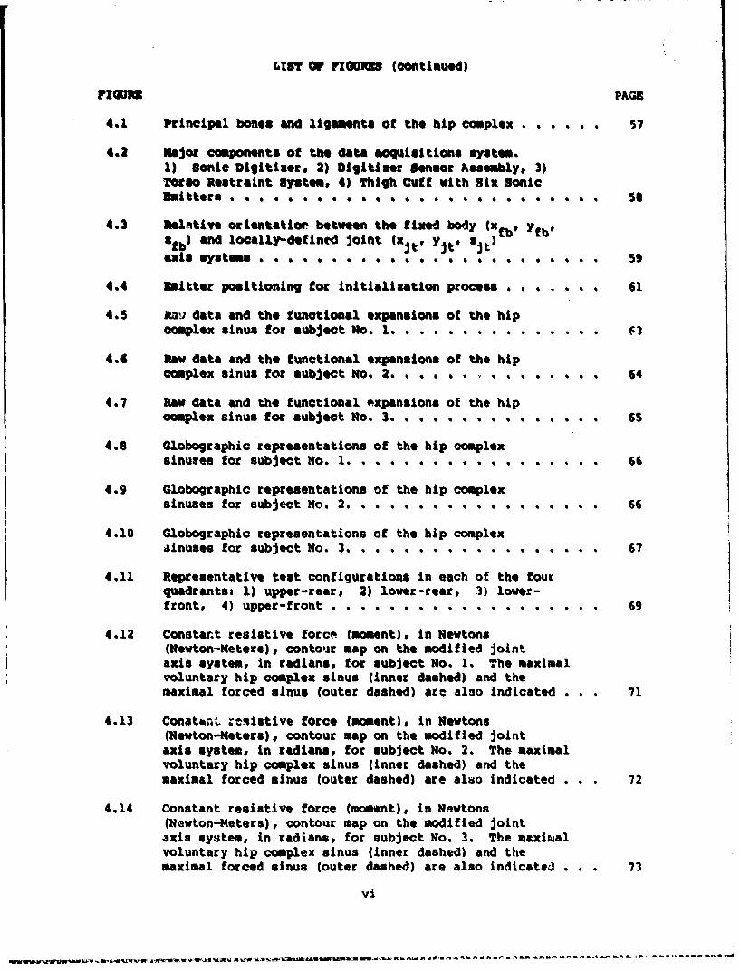
LIST OF FPIRNS (coontinued)

4.1 Principal bones and ligments of the hip complex . . . . . . S7

4.2 Major components of the data aoquisitions system.1) Sonic Digitiete, 2) Digitizer Sensor Assembly. 3)Torso Restraint System, 4) Thigh Cuff with Six Sonicftittersn a 0 a a 4 , 0 * , a , * * . . , 0. . . 50 006aI s

4.3 Relative orientatioa between the fixd body (xfb ,fb'afb) and looally-defined joint (xjt. at# 'j t)axis systems . . . . . . . . . . . . . , . . . 9 . , . . . . 59

4.4 EMitter positioning tot initialisation process . . . . . . 61

4.5 Mu data and the functional expansions of the hipcom~plex sinus for subject NoI. 1. . . . . .. .. .. . .. 63

4.6 Raw data and the functional expansions of the hipomplex sinus for subject No. 2.. .. . . . . .. .. . 64

4.7 Raw data and the functional expansions of the hipcomplex sinus for subject No. 3. .. ........... 65

4.8 Globographic representations of the hip complexsinuses for subject o. 1 . ............ ... 66

4.9 Globographic representations of the hip complexsinuses for subject No. 2. . . . . . . . . . . . . . . . . . 66

4.10 Globographic representations of the hip complexminuses for subject No. 3. . . . . . . . . . . . . . . . . . 67

4.11 Representative test configurations in each of the fourquadrantst 1) upper-rear, 2) lower-rear, 3) lower-front, 4) upper-front .............. ..... 69

4.12 Constant resistive force (moment), in Newtons(Newton-Meters), contour map on the modified jointaxis system, in radians, for subject No. 1. The maximalvoluntary hip complex sinus (inner dashed) and themaximal forced sinus (outer dashed) are also indicated . . . 71

4.13 Conatanmt rehstive force (moment), in Newtons(Newton-Meters), contour map on the modified jointaxis system, in radians, for subject No. 2. The maximalvoluntary hip complex sinus (inner dashed) and themaximal forced sinus (outer dashed) are also indicated . . . 72

4.14 Constant resistive force (moment), in Newtons(Newton-Meters), contour map on the modified jointaxis system, in radians, for subject No. 3. The maximalvoluntary hip complex sinus (inner dashed) and themaximal forced sinus (outer dashed) are also indicated . . . 73

vi

t

List aI Pi •. S (continued)

IFIGUitRE&

4.15 IMW data and the fitted-curves (dEM from Figure 4.12)for nwCeal onstant-0 s"ePs . .al.e .* . 74

4.16 Globographic nqresentations of the maximal voluntary(inner curve) a"d forced (outer curve) sinuses forsubject No. 1. . , . ., , . . , ., ., 6 , 0 . . * , , a 75

4.17 Globographic repcosentations of the maximal voluntary(inner curve) and forced (outer curve) sinuses forsubject tN. 2 . . . . . . . . . . . . . . . 4 . . . . . . . 0 75

4.18 Globographic reWesentations of the maximal voluntary(Inner curve) and forced (outer ourve) sinuses forsubject No. 3. . . . . . . . . . . . . . . . . . . . . . . . 74

4.19 Hip complex sinuses for all ten subjects (dotted curves).

solidcurves ar tfor 5 and .8. . . . . . . . .a . 76

4.20 Globographic representations of & and + Be . .a. . . . 78

4.21 5 And I + 8 a for two different runse % , . . . . . . . . . 78

4.22 Ccefidence Interval (CI) for the population mean, g . . . . 79

4.23 Globographic representation of the Confidence Intervalfor the population manm. . . .... . . . .... 79

4.24 Sample means of the passive resistive property, maximumvoluntary sinus (inner dashed), and maxim= forced sinus(outer dashed) . ....... . . ..... . .... . 82

4.25 Globographic representations of the sample means of themaximum voluntary and forced sinuses . . . . . . . 82

S.1 lKinematic and force application tests for the elbowGompl exS. . . . . . , . . . . . . . 84

5.2 Relative orientation of the mean joint axis system,or' the fixed-body axis system, (xfb Yfb' lfb) andthe torso axis system. (xtat yts* ats) . ......... 85

5.3 Relative orientation of the fixed-body (xfbe afb' fb) andthe locally-defined joint (xjk, Y¥tt st) axis systems . . 87

5.4 Raw data and the functional expansions of the hunero-elbowcomplex sinus for subject No. 1 . . . . . . . . . . . . 89

5.5 Raw data and the functional expansions of the humero-elbowcomplex sinus for subject No. 2 .............. 90

vii

muk~mmm~m•I~l2WUWa•-- ... .

LIST Of FIQIRMS (continued)

FZ=M PAGE

S.6 Raw data and the functional expansions of thehumeto-elbov complex sinus for subject No. 3 . . . . . . . . 91

5.7 Globogtaphic representation of Pig* S.4. . . . 92

5.0 Globogtaphic representation of Fig. S.5 . ..... 93

5.9 Globographic tepresentation of Fig. 5.6. . . , . . 94

5.10 Raw data and functional expansions of the passiveresistive property for subject No. I ... . . . . 95

5.11 Raw data and functional expansions of the passiveresistive property for ubjeotNo .n . .a . . .0 4 0 . 95

5.12 Raw data and functional expansions of the passiveresistive property for subject No. 3...... . . . . . 96

5.13 Numero-eObov complex sinuses for all ten subjects.

Solid curves are for & and 9 + s. a . a ... .. . . 0 . 97

5.14 Globographic representations of and + So 97

5.15 9 and & _+ S8 for two runs . . . . . ....... 98

5.16 f(Qr) for all ten subjects. Solid curves ate forSand If_+ sf . . ... . . . .,. . . .. 99

B.1 Flownhart for data acquisition and associated dataanalysis.. . . . . . . . . . ... 105

LIST OF TABLES

TABLE PAGE

3.1 Centers and radii of the best-fitted spheres ond (n 0 n)for all ten subues .... s......... ........ 19

3.2 Subject-based coefficients of the shoulder complex sinusesfor all ten subjects .................. . 37

3.3 Space-based coefficients of the shoulder complex sinusesfor all ten subjects . .................. . 38

3.4 Subject-based coefficients of the passive resistiveforce (moment) data for all ten subjects . . . . . . . . . . 49

3.5 Space-based coefficients of the passive reqiqt-ve !orce(moment) data for all ten subjects ... ........ . . 50

viii

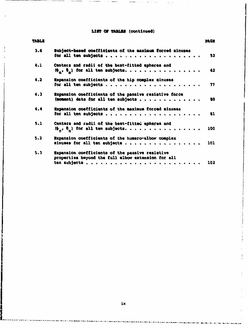
LIUT Of TAIKLS (continued)

TABUE MAE

3.6 Subjeat-based ooefficients of the maximum forced sinusesfot all ten subjets . . . . . . . . . . .... 52

4.1 Centers and radii of the bast-fitted spheres and(on. t n) for all ten subjets. . . . .* .. .,. . . . .% 62

4.2 Expansion coefficients of the hip complex sinusesfor all ten subjects . , . . . . . • . ... a.... .. • 77

4.3 Expansion coefficients of the passive resistive force(moment) data for all ten subjects . % . . . .a . . . . . to

4.4 Expansion coefficients of the maximum forced sinusesfor all ton subjects ... .. , a .6 .. .. .0 el 000000 6

3.1 Centers and radii of the best-fitte" spheres and(OnI On) for all ten subjet.... . .. ......... 100

5.2 Expansion coefficients of the humero-elbov complexsinuses for all ten subjects. . . . . . . . . . . . . . . . 101

5.3 Expansion coefficients of the passive resistiveproperties beyond the full elbow extension for allton subjects . . . . . . ................. 102

ix

1. INTRODUCTION

S~1.1 Background

Mathematical modeling and simulation of biomechanical system crash

response play an economical anA ,ersatile role in the understanding ofinjury mechanism. In quantitative gross biodynamic motion studies,

cognizant of the high coat of conducting experimental research with human

cadavers and/or anthropomorphic dummies, biomechanicians have turned

their attention to th^ utilization of computer-based mathematical models

of the total human body since the advent of high speed computer

technology. Among these models, the most popular and sophisticatedversions are articulated and multisegmented to simulate the total human

body as a linked structure made up of rigid bodies. Fig. 1.1 shows a

typical three-dimensional model consisting of fifteen segments.

Representative three-dimensional models developed in various research

* centers include six-segment model of UMTRI (formerly called HSRI)

(Robbins et al., 1972), twelve-segment models of TTI (Young, 1970) and of

UCIN (Huston et al., 1974), and fifteen-segment model of Calspan (Fleck,

1975). With some addittonal features, the Calspan model is also beingused by the U.S. Air Force under the title of Articulated Total Body

(ATB) model in aerospace related applications.

In these models, the equations of motion are formulated by usingeither the Newtonian approach or Lagrange's equations, Euler's rigid body

equations, and Lagrange's form ol d'Alembert's principle and solved byvarious methods such as Runge-Kutta or Predictor-Corrector numerical

integration scheme. Joints are modeled as either the ball-and-socket

type with three degrees of freedom or the hinge type with only one degree

of f reedom. Resistive force responses beyond the loint stop contour

(maximum range of motion) are modeled as one or a combination of the

following simple mechanical components: a linear spring, a non-linearspring, a Coulomb friction damper, and a viscous damper. Furthermore,

joint properties, i.e.,stop contours and resistive force characteristics

are estimated ar.', in some cases, even assumed. A thorough review of

both two- and t'Acee-dimensional mathematical models simulating biodynamic

response of the human body along with the associated experimental

validation studies performed, was provided by King and Chou (1976).

11

J4j ~Nl

0 J3 0

RUA UT LUA

2 14

CTJ12 2 0J 14

RLA J1 LLA13 LT 1 1i

J s 0 0 Ji

RLL LLL

7 10

J7 0 1

F JLo

Fig. 1.1 A fifteen-segment model of the total human body

Obviously, the effectiveness of these multisegmented mathematical

models in accurately predicting in-vivo biodynamic responses, depends

upon the individual segment properties such as center of gravity, moment

of inertia, geometry, etc., and more heavily upon the biomechanical joint

properties between any two linked segments. In particular, the resistive

force properties of the joints play a direct and significant role in the

understanding of injury mechanisms 'as well as in the prediction of

ianjury. Although a number of studies have supplied data for model

segment properties (Hatme, 1980; McConville et al., 1980), data on

btomechanical joint properties are comparatively sparse (Steindler, 1973)

and limited: (Enginf 1980; Engin, 1984). of course, a complete data base

for the biomechanical joint properties should undoubtedly include a

statistical analyst- to account for the intra- and inter-subjectvariations.. The more sound the joint property data base is, the more

realistically the multisegmented anthropomorphic dummies and computer-

based mathematical total-human-body models can be constructed and

formulated.

1.2 Definitions of Joint'Sinus and Globographic Representation

Throughout this dissertation, the terms joint sinus and globographic

representation (first used by Dempster, 1965) will be repeatedly used in

the discussion of joint properties. Since these two: terms are not

commonly known, let us give their definitions to avoid possible

confusion.

Joint Sinus: the maximum range of angular motion permitted by the

moving member of a joint while the other member is rigidly fixed. The

joint should possess at least two degrees of freedom such that the moving

toember sweeps out a conical concavity within which the joint structures

permit all possible movements.

Globographic representation: a graphical method of representing a

joint sinus upon the surface of a globe with meridians and parallels

which define a grid pattern of the angular spherical coordinates with

respect to a fixed axis system attached to the rigidly fixed member; the

center of the globe is positioned at the functional center of the joint.

In this study, we will also use another method to represent a joint

sinus, namely, a single-valued functional relationship between the two

3

spoer ical angles of the joint sinus. While the globographic

representation provides a physically. meaningful plot for *he joint sinus,

the single-valued functional relationship condenses the joint sinus data

.nto a functional expansion form for easy incorroration into the existing

three-dimensional multisegmented models of the total human body.

1.3 € ofResearoh

The primary goal of this research program 'is *to provide/establish

proper biomechanical joint property data/databases pertinent to the human

shoulder, hip, and humero-elbow complexes for incorporation. into the

existing three-dimensional muAltisegmenkted models. A recently developed

new kinematic data collection methodology by means of sonic emitters and

a data analysis technique based on selection of the "most accurate" axis

system from an overdeterminate number of sonic emitters on the moving

segment *(Engin et al., 1984a), were applied and extended. The passive

resistive force data were collected by utilizing a three-dimensional

multiple-axis force and moment transducer whose calibration and

application with sonic emitters was desuribed iot a previous work (Engin

et al., 1984b). System accuracy of this data acquisition technique was

also previously documented by performing:

(1) Error analysis on two types of controlled linear translational

motion; a rather high degree of accuracy was attained (Engin et al.,

1984a).

(2) Joint sinus simulation tests on a mechanical revoluto-hinge Joint;

even with high degrees of acoustic blockage, an average of 86.51% of

the calculated joint centers fell within 1.46 cm. from the true

joint center (Engin and Peindl, 1986).

(3) Forced abduction simulation tests (sweeping-type motions) on the

same mechanical revolute-hinge joint.- an average of 81.55% of the

calculated joint centers fell within less than 0.5 cm. from the true

joint center (Engin and Peindl, 1986).

The system accuracy tests described above, demonstrate that the

sonic digitizing technique can be employed to perform fairly complicated

three-dimensional rigid body kinematic analysis when used in connection

with an overdeterminate number of sonic emitters. In this study, the

performance of the data acquisition system and efficacy of the associated

4

data analysis methodology is culminatingly assessed by observing good

repeatability of the joint sinus sample means from different runs on ten

subjects.

Finally, a statistical data base for the biomechanical joint

poperties is established in a systematic way for a special population,

namely, the male population of ages 18 thru 32 possessing neither

"musculdskeietal abnormalities nor any history of trauma in the joints

studied herein. Ten, subjects were randomly chosen to form the sample

with emphasis placed on choosing subjects whose anthropomtry

approximates the average for the above-defined population. Selected

anthropometric measurements:o6f these subjects are given in Appendix A.

The sample mean and sample standard deviation as well as the confidence

intervals for the population mean,. and population standard deviation were

obtained in a systematic way and were expressed in functional expansion

form relative to a locally-defined joint axis system as well as relative

to the fixed-body axis system in the form of globographic representation.

It is believed that this is the fir•t attempt to establish a

statistically meaningful data base for the 'biomechanical properties of

the major human articulating joints for the purposes of incorporation

into the multisegmented mathematical models of 'the total human body.

2. XIMWT!CS BY MAN OF AN MOW I3UINATU •M OF SONIC EMITTERS

In this chapter, we shall fLacuss the general approach to studying

the three-dimensional kinematics of a typical joint complex# which links

two body segments, by means of an ovordeterminate number of sonic

emitters. The following chapters will apply this methodology to

deternine the maximum voluntary ranges of motion and passive resistive

properties beyond them for the shoulder* hip, and humero-elbow complexes.

2.1 Review of the Sonic Dicitilina Technique

Sonic digitizing is the process of converting information on

position via sound waves to digital values in a form suitable for data

tranamiscion, stcrage, and processing. The sound waves, which are audible

impulses of a specific frequency, are generated by an electrical arc at

the tip of the emitter powere.J by the GP6-3D Sonic Digitizer manufactured

by Science Accessories Corporation. 'Point* microphone sensors capable

of detecting this specific frequency of sonic impulses are used to receive

the sound waves. By multiplying the transit time required for a sound

wave to reach a microphone sensor with the speed of sound in still air,

the sonic digitizer converts the distance from the emitter tip to the

"point" microphone sensor (to be referred to as slant range distance)

into digital values. These digits are then transmitted to a PDP-11/34

minicomputer for data analysis and storage.

By applying this sonic digitizing principle, a rigid planar

rectangular sensor board/assembly with four "point' microphones/sensors

(A, B, C, D) arranged at the corners, as shown in Fig. 2.1, was

constructed (Engin and Peindl, 1985). Tha purpose of this set-up is to

convert the four slant range distances of a sonic emitter, which defines

a point in the 3-D space, into regular Cartesian coordinates suitable forperforming kinematic analysis. Note that only three slant range

distances are needed for the conversion. The fourth sensor is used for

spare purposes. During conversion analysis, the computer program is

designed to examine all four slant range distances, select the three

smallest, and discard the fourth. In the special case where one of the

slant range distances is zero, namely, the sonic emitter is totally

blocked from being detected by one of the four microphone sensors, the

zero reading is disregarded.

6

- SONIC EMITTER

IBy- AXIS

C SENSOR

G P11 ASSEMB3LY

"E"' * F B

A (O) H x-AXIS

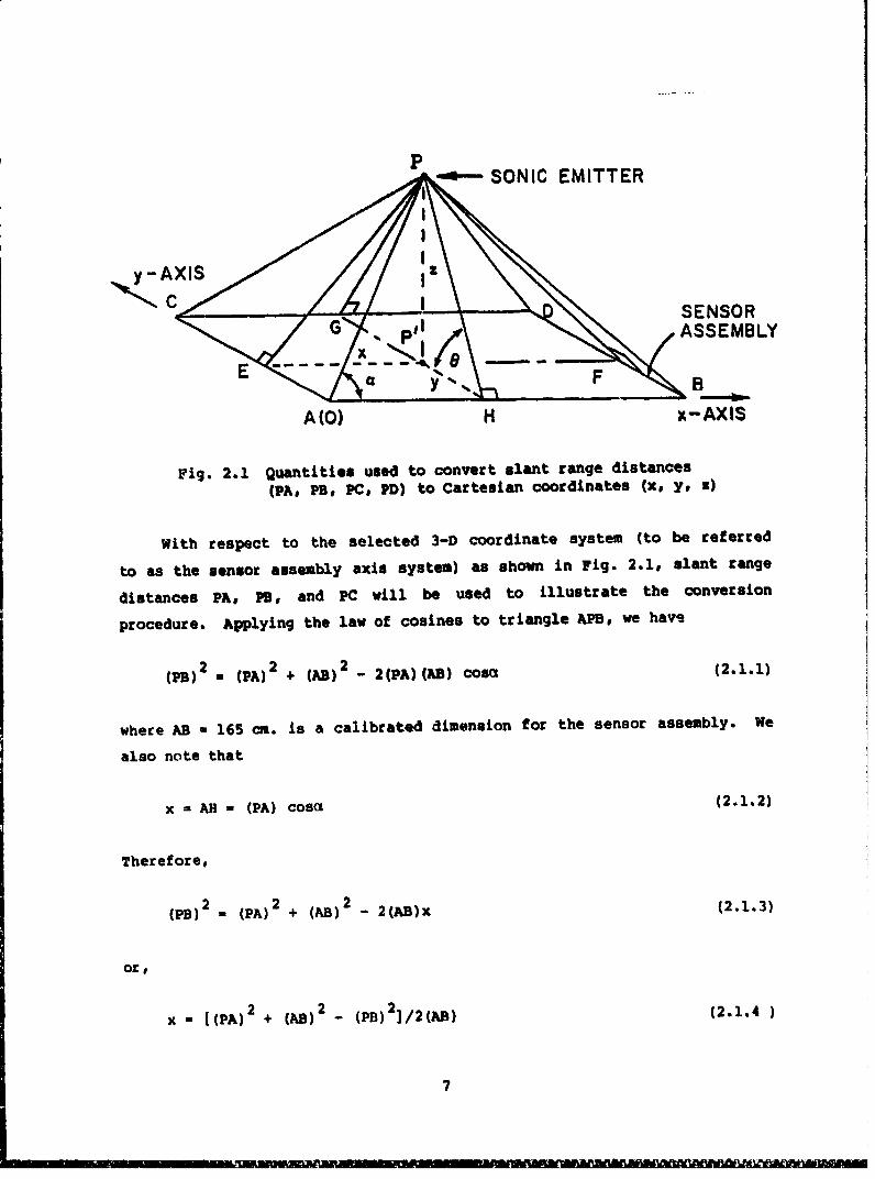
Fig. 2.1 Quantities used to convert slant range distances(pA, Ps, PC, PD) to Cartesian coordinates Nxo y, s)

With respect to the selected 3-D coordinate system (to be referred

to as the sensor assembly axis system) as shown in Fig. 2.1, slant range

distances PA# PB, and PC will be used to illustrate the conversion

procedure. Applying the law of cosines to triangle APE, we have

(PB)2 , (pA)2 + (AB) 2 _ 2(PA)(AB) cosa (2.1.1)

where AB - 165 cm. is a calibrated dimension for the sensor assembly. We

also note that

x - AH - (PA) cosa (2.1.2)

Therefore,

2 2 2(.1)(PB) . (PA) + (AB) - 2(AB)x (2.1.3)

or#

x - H(PA) 2 + (AB) 2 _ (PB) 2 ]/2(AB) (2.1.4

7

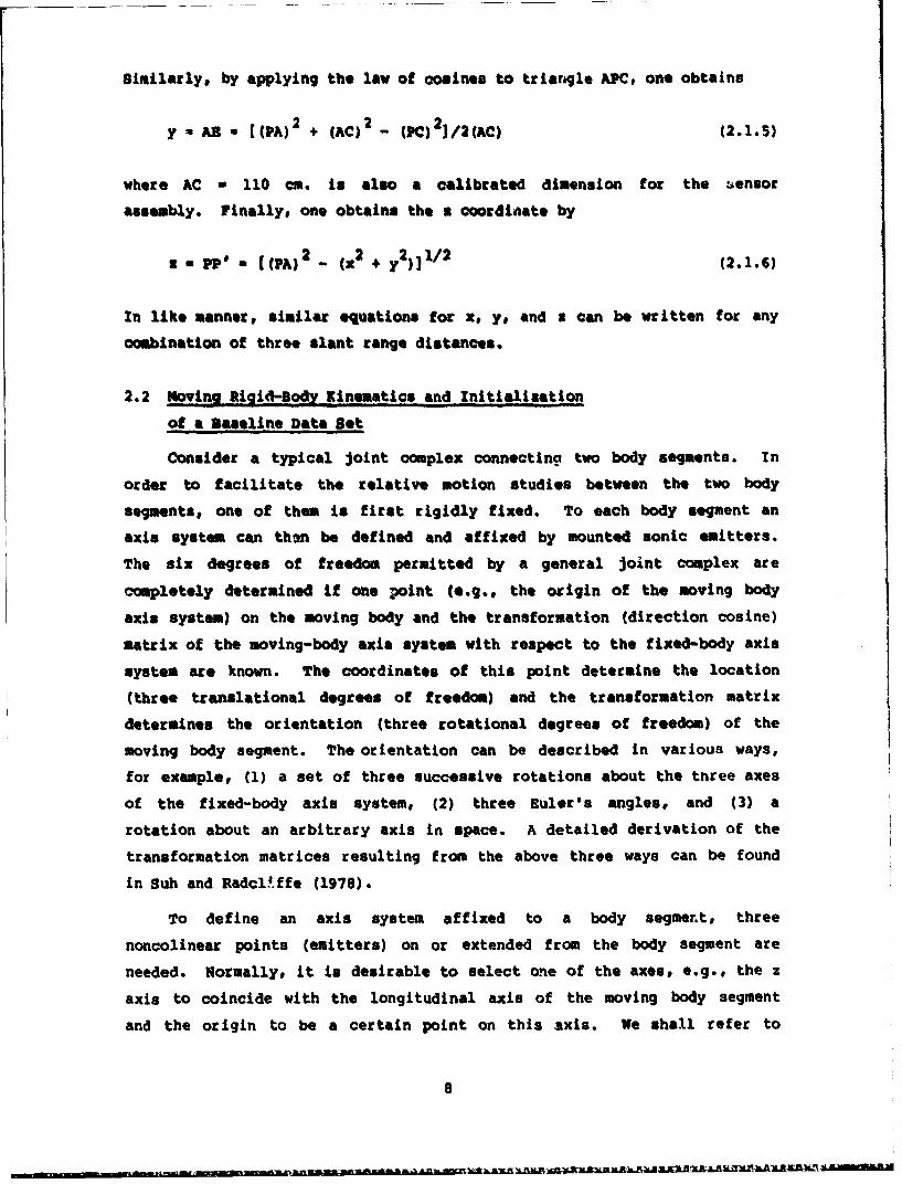
Similarly, by applying the law of cosines to triaragle ApC, one obtains

y M AR , [(PA) 2 + (AC) 2 - (PC) 21 /2(AC) (2.1.5)

where AC a 110 cm. is also a calibrated dimension for the -ensor

assembly. Finally, one obtains the a coordinate by

2 a ppOa [(PA) 2 _ (x2 + y 2 )]1/ 2 (2.1.6)

In like manner, similar equations for x, y, and x can be written for any

combination of three slant range distances.

2.2 Moving Rigid-Body Kinematics and Initialisation

of a Baseline Data Set

Consider a typical joint complex connectina two body segments. In

order to facilitate the relative motion studies between the two body

segments, one of them is first rigidly fixed. To each body segment an

axis system can thon be defined and affixed by mounted sonic emitters.

The six degrees of freedom permitted by a general joint complex are

completely determined if one point (e.g., the origin of the moving body

axis system) on the moving body and the transformation (direction cosine)

matrix of the moving-body axis system with respect to the fixed-body axis

system are known. The coordinates of this point determine the location

(three translational degrees of freedom) and the transformation matrix

determines the orientation (three rotational degrees of freedom) of the

moving body segment. The orientation can be described in various ways,

for example, (1) a set of three successive rotations about the three axes

of the fixed-body axis system, (2) three Euler's angles, and (3) a

rotation about an arbitrary axis in space. A detailed derivation of the

transformation matrices resulting from the above three ways can be found

in Sub and Radclffe (1978).

To define an axis system affixed to a body segmer.ts three

noncolinear points (emitters) on or extended from the body segment are

needed. Normally, it is desirable to select one of the axes, e.g., the z

axis to coincide with the longitudinal axis of the moving body segment

and the origin to be a certain point on this axis. We shall refer to

8

this type of axis systems as tie longitudinal (or long-bone) axis

systems, 3owever, sJnce the sonic digitizing technique is Iapplied in

this study, total and partial acoustic blockage may occur to pi:oduce zero

and inaccurate readings for one, or two, or even all three sonic emitters

used. Note that in defining the fixed-body axis syitem, this difficulty

can always be avoided by adjusting the sensor assembly to an optimal

'view' of the three emitters since these emitters are not moving. In the

case of the moving body segment, it Is desirable to continuously monitor

the moving body axis system while performing joiat property experiments.

As a result, total or partial acoustic blockage becomes in~evitable for

some *bad* positions where sound waves must travel around t:he emitters'

bases or the moving body segment itself. Therefore, it in necessary to

collect redundant data so that sero readings from individual emitters

would not affect kinematic analysis. Obviously, we would select the

"most accurate" three emitters in cases where more than three emitters

produce non-zero readings.

From experimental experience, six emitters are moat suitable for the

redundancy process. Seven or more emitters would dramatically increase

computing time without noticeable improvements In accuracy, while four or

five emitters do not provide a sufficient spare. Note that If six

emitters are used, a total of 20 (C(6, 3) a 311 ) different axis systems

can be constructedi if seven emitters are used, a total of 35

(C(7,3) - ) different axis systems can be constructed.

It is advantageous to arrange the six sonic emitters

circumferentially and more or less equally-spaced around the moving body

segment. (In reality, the six emitterv are fizst put on an orthotic cuff

which, in turn, is strapped circumferentially to the moving body

segment). The advantage is that, by doing so, we have reduced the number

of 'bad' positions to a minimum and also provided the moving body segment

with the largest amount of freedom to reach all allowable ranges of

motion. However, such an arrangement of the six emitters makes them

unsuitable for direct construction of the longitudinal axis system as

normally desired. One way of resolving this inconvenience is to

establish the relationship (to be explained later) between the six

emitters and the longitudinal axis system directly constructed by three

properly positioned emitters before performing kinematic data collection

9

and analysis. Since this rclationship is Invariant, i.e., it does not

depend upon the orientation/location of the moving body segment. or the

sensor assembly, its accuracy can be checked against pre-calibrated inter-

emitter distances to within It of error by adjusting the relative

orientation and location between the moving body segment and the sensor

assembly to an optimal "view'. This procedure to called initialisation.

The initialized data seo, which is reliably accurate, also provides a

baseline for the selection of the "most accurate" longitudinal axis

systems (will be explained in detail in the next section) for the

continaously collected kinematic data whose accuracies are uncontrollable

due to partial and/c': total acoustic blockage and motion during kinematic

data collection. This baseline contains the interrelationehips among the

six sonic emitters on the moving body. The following explains how the

interrelationships among these nine emitters (three for defining the

longitudinal axis system, six on the moving body segment) are

initialized.

First, the coordinates of the nine emitters are calculated in terms

of the sensor assembly axis system. Next, a total of 20 axis systems ik

defined by calculating the direction cosine matrices Ain (1 i < 20) with

respect to the sensor assembly axis system from all possible combinations

of any three out of the six moving-body emitters. Note that these axis

systems can always be obtained since all the six emitters are arranged In

such a way that no three of them are colinear, i..., three mutually

orthogonal unit vectors can always be found. The longitudinal axis

system is similarly defined by calculating its direction cosine matrix,

B I, with respt-t to 4he sensor assemvly axis system. Next, the

transtormation (dirertion cosine) matrix describing the ith axis system

relative to the jth axis system (1 < i < j < 20) is then calculated by-J. TAij = As A As A = A A , where A and A are theiis sj is js is js is j

t,,ansforiG.tion matrices describing the ith and jth axis systems relative

to the sc~isor assembly ax&s system, respectively. Note that these 190

(C(20,2) = d:-) transf--ranation matrices relating each of the 20 axis

systems relative to every other system are an intrinsic geometric

property Df the six moving-body emitters and are in.lependent of the

sensor assembly axis system. Second, the distances between the origins

of any two of the 20 axis systems, Dij (1 < i < j < 20) are initialized.

Obviously, these 190 scalar quantities are also Intrinsic and independent

10

of the sensor assembly axis system. Third# the coordinates (positionvactors) of the origin of the longitudinal axis systemo with respect tothe 20 moving-body axis systems art also Initialized by A is is(1 4 1 420). where in is the position vect~or fleas the origin of the ith

axis system to the origin of the longitudinal axis system expressed interm of the sensor assembly axis system. Uote, that these 20 vectors actalso intrinsic and Independent of the *seso assembly axis rtystem duringthe initialisation process. Toast# the transformation matrices of thelongitudinal axis system with respect to each of the 20 moving-body axissystems are initialized by is A T* *4 (1l < 20)'. Not*that these, 20 matrices act also independent of the sensor assembly axissystem. All the Initialized data are Stared In the computer andretrieved for the selection process and detertmination of the longitudinalaxis system aon the moot accarate3 moving-body axis system is selected.

2.3 Selection of the *Moet ficcurate* Axis System an the NOVIIN Body

The Initialised data set discussed in the previous section form abaseline for the selection criterion since these data are obtained In an

optimal view of the sensor assemudgy aid their accuracy can be wellcontrolled. nomever, fom a typical kinematic test# with the moving bodysegment In notion, the accuracy is uncontrollable. Since the Initializeddata set is independent of the sennso assembly axis system, It can beused for any position and orientation of the moving body segment inselecting the 6most acaurateg moving-body axis system for determinationof the desired longitudinal axis system which conveniently describes thecomplete kinematics of the moving body segment. The sequential firingrate of the six moving-body emitters Is set at 7 records per second, andthe motion speed of the moving body segment is maintained atapproximately 60 arc/sec. One record is defined as a complete sequentialfiring of all the six moving-body emitters from which one set ofkinematic data with respect to the fixed body axis system is determinedthrough coordinatte, transformation and vector analyses.

The choice Of the 'Met accuCateo axis system on the moving bodysegment during a kinematic test is made on a record by record basis. Foreach record of the kinematic data, the coordinates of the six moving-body

emitters (assuming that all of them give good readings, i.e.,, none, of

/

them is totally blocked from sensor view) are first used to obtain the

intrinsic matrix interrolationships between any two of the 20 cxis systema

as described in the initialisation process. if there were no errors in

the kinematic measurements# and the orthotic cuff remains rigid, then we

should obtain the equalitioes

(M.ljlkinematl€ (A Winitial or

(Aijlkinematic (ijinitial .2 (l'i•_ 20) (2.3.1!

and

(Dip)kinoatic " ) initial. or

(DiJ)kinemati." - ij)initiai * 0 ( 1 !.. i 20 (2.3.2)

where I is the 3 x 3 identity matrix. This& however#, i not the (Ase for

a typical kinematic test due to such factors as motion during data

collection, changes in the emitter's orientations vith respect to the

sensor a&sotly* or the partial acoustic blockage of Individual emitters

by the fixed body or the moving body segment itself. Therefore, we

obtain the folioving inq.ialitieas

(&Ij)kinematic (AJ) initial ij ( 1- 20 ) (2.3.3)

and

(Dij)kinematic - (Dis initial - 6 0 0 1 i J < j 20 -(2.3.4)

where Gj is a general matrix with off-diagonal terms, and 6 is anij iiapparent dislocation (translational shift) between the origins of the ith

and jth axis systems. The general matrix can be considered as a rotation

rmatrix describing an apparent rotational shift between the ith and the

jth axis systems from their initialixed interrelationship. It should be

pointed out that both the dislocation and rotational shift are a relative

measure of the errors involved. These errors are not correctable, i.e.,

we cannot pinpoint the absolute errors. Nevertheless, we have at least a

12

relative sense of how much they are so that we can always select the

"Most accuraten data met. Therefore, a good relative indication of the

magnitude of the rotational shift is to consider the amount of rotation t

YL,# introduced by 0i1. about an axis. To calculate yijt we notice that

the rotation mtrix describing a rotation of amount * about an axis

whose orientation is specified by the direction cosines of a unit vector

u- ux 0ye us) is (Uuh and Radcliffet 1976)

uSloe)4oslcok'ss (2.3.5)

Sutuing up the diagonal terms of the matrix R and noting that

u2 + u 2 + u 2 1, we obtain

a - Cos-I 1 (tiR - 1)) (2.3.6)

where trR iU the trace of R3 i.e., the sum of all the three diagonal

terms of the matrix R. Applying this equation to the general nmatrix GOO

we find

Yjj a Cos"1 tr Gij - 1)] 1 (2.3.7)

Since the orthotic cuff is made of rather rigid steel and during the

kinematic test there is essentially no force applied on it, we attribute

both the translational and rotational shifts to motion during the emitter

firing sequence and/or measurement inaccuracies due to partial acoustic

blockage.

For each kinematic data record, if one assumes the jth axis system

to be accurate, then the ith axis system has obviously introduced both

errors, i.e.. 6 and yij" If we then calculate, for each axis system,

the root mean square error, CV, by assuming all the other 19 axis systems

are accurate, as

Y = ~ (iS) + NJ 1 _< i _<20 ( 2.3.8)

JullJ1i

13

pote that, in this equation. Yj should be thought of on the arc length

obtained when yis Multiplied by a unit length), the axis system which

exhibits the smallest a has obviously undergone the least qpparent shift

(rotational and translational) with respect to all the other axis system

as initialimed. PrCo a statistical point of view, this axis system has

the highest pcobability of being the most accurate as compared to the

initialised geometry.

Por each kinematic data record# the "most accurate" axis system on

the moving bady segment to then uced to calculate the o&igin and the

direction cosine matrix of the longitudinal axis system via the

initiallsed data, i.e.. J, and B,,. Or. stating It In another manner, we

are monitoring the desired longitudinal ai's system via a versatile

medium, i.e., the six emitters on the moving body segment.

14

3. BIO•IICHRICKL PROPERTIES OF THE HUMAN SHOULDER COMPLEX

3.1 Introduction

In multisegmented mathematical models of the total human body, the

most complicated and least succesesflly modeled joint has been the

shoulder complex mainly due to the lack of an appropriate biomechanical

data base as well as the anatomical complexity of the shoulder region.

The term "shoulder complex" refers to the combination of the shoulder

joint (the gl.enohuueral joint) and the shoulder girdle which includes the

clavicle and scapula and their articulations. Therefore, in discussing

the joint sinus of the shoulder complex, it is more appropriate to use

the term *shoulder complex sinus" to designate the range of extreme

allowable motion of the humerus with respect to torso. It is important

to make this distinction since it is possible to define joint sinuses for

various skeletal components of the shoulder complex. An anatomical

description and a brief account of studies on the shoulder complex was

provided by Engin (1980) and more details can be found in standard text

books (Steindler, 1973; Gray's Anatomy, 1973; Norkin and Levangie, 1983)1

thus they will not be repeated here.

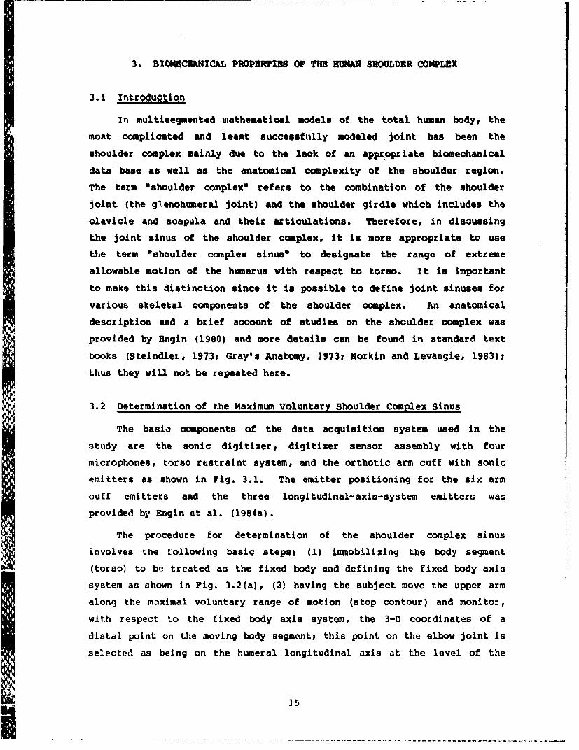
3.2 Determination of the Maximum Voluntary Shoulder Complex Sinus

The basic components of the data acquisition system used in the

study are the sonic digitizer, digitizer sensor assembly with four

microphones, torso restraint system, and the orthotic arm cuff with sonic

emitters as shown in Fig. 3.1. The emitter positioning for the six arm

cuff emitters and the three longitudinal-axis-system emitters was

provided by Engin et al. (1984a).

The procedure for determination of the shoulder complex sinus

involves the following basic stepst (1) imnobilizing the body segment

(torso) to be treated as the fixed body and defining the fixed body axis

system as shown in Fig. 3.2(a), (2) having the subject move the upper arm

along the maximal voluntary range of motion (stop contour) and monitor,

with respect to the fixed body axis system, the 3-D coordinates of a

distal point on the moving body segment; this point on the elbow joint is

selected as being on the humeral longitudinal axis at the level of the

! ].5

Fig. 3.1 Subject in the torso restraint system and the armcuff with six sonic emitters

humeral conrdylar maximal width, (3) fitting the 3-D coordinates to a

sphere using a least-squares technique, thus establishing a center for

the best-fitted sphere and an idealized link length (radius of the

sphere), (4) fitting a plane to the same 3-D coordinates using a least-

squares Lechnique; the normal to this plane (specified by the spherical

coordinates (n , en) as shown in Fig. 3.2(b)) establishes the pole of an nlocal joint ax.' s system (zit-axis) about which the shoulder complex

sinus, designated by the spherical coordinates (ý, 0) of the vector

connecting the center of the sphere with the dis•al elbow point, can be

ezpressed as a single-valued functional relationship, i.e., 0 =e().

16

since the origin of the fixed body axis system in inaccessible, a

relative axis locator device (RALD) (Engin et al., 1984) is used to

Low

-- (0)

Xjt

TI 0 .VtWR

Ypm

SItZfb Xfb

Zfb(b)Zb

Fig. 3.2 (a) Selected origin and axis system (Xfb' Yfb' zfb]of the fixed segment (torso).

(b) Relative orientation of the fixed body (xfbW Yfb'

zfb) and locally-defined joint (xjte Yjt' z~t)axis systems.

17

locate the origin and define the transformation matrix of the fixed body

axis- system in terms of the miorophone/sensor assembly axis system. The

accuracy of these data can always be maintained within It of error

against pre-calibrated dimensions by adjusting the orientation and

location of the microphone/sensor assembly. Of course, this adjustment

should also take into account the orientation and/or position of the arm

cuff in order to obtain the best kinematic data even though an

overdeterminate number of sonic emitters and a "most accurate" selection

criterion are used.

Table 3.1 lists the centers and radii of the best-fitted spheres and

(n' ,n) as well as their ample means and sample standard deviations for

all ten subjects. The mean values for (0 n en) shall be designated as

i0' am) and the corresponding joint axis system shall be referred to as

the mean joint axis system.

Before the test, each subject was instructed to move his upper arm

along its maximum range of motion boundary in a counterclockwise motion

as viewed from the sensor assembly. He was also instructed to displace

the arm distally along its longitudinal axis as far as possible at all

times while circumscribing the joint sinus. Preferred rotation of the

upper arm about its longitudinal axis was left up to the discretion jf

subjects in obtaining the maximal contour. Several sweeps of this type

were performed before data were collected so that the subjects could

experiment with obtaining the largest possible range of motion. In order

to help maintain a constant rate of motion, a large clock with an easily

visible second hand was placed in front of the subject. The subjer C was

instructed to imagine his humerus as the second hand, and to synchronize

his joint sinus circumscription with the clock's 60 second sweep. In

this manner, three test runs (sweeps) were collected for each subject.

To consolidate the enormous volume of experimental raw data into a

form readily usable by the multisegmented total-human-body models

currently in use, functional expansions for the shoulder complex sinuses

are desirable. This is also the reacon why we want to represent the

shoulder complex sinus in a single-valued functional relationship, i.e.,

e = e(-), with respect to the locally-defined joint axis system. It will

be shown in Section 3A4 that the functional expansions also greatly

facilitate the statistical. analysis.

18

Table 3.1 Centers and radii of the best-fitted spheres and (@n )for all ten subjects n n

SUBJWc CMNTER (ce) PADIUS en onNO. Xfb Yfb 4fb (N) (deg.) (deg.)

1 8.85 14.92 -26.91 36.75 57.37 72.24

2 3.30 10.01 -25.25 35.37 56.52 77.32

3 5.45 15.50 -25.76 34.19 55.51 •1.61

4 9.67 16.75 -33.67 36.28 59.72 83.20

5 2.53 13.78 -24.77 32.09 58.82 79.53

6 3.78 15.48 -25.39 32.83 62.58 77.86

7 7.10 16.51 -24.68 32.18 59.43 78.87

8 4.51 12.59 -24.94 35.25 57.12 77.90

9 6.88 17.27 -24.62 31.77 60.98 84.31

10 1.88 16.25 -25.85 33.96 64.87 77.93

Sample 5.40 14.91 -26.19 34.07 59.29 79.08Mean

Sample 2.66 2.23 2.72 1.81 2.90 3.42St. Dev.

19

N A SJ

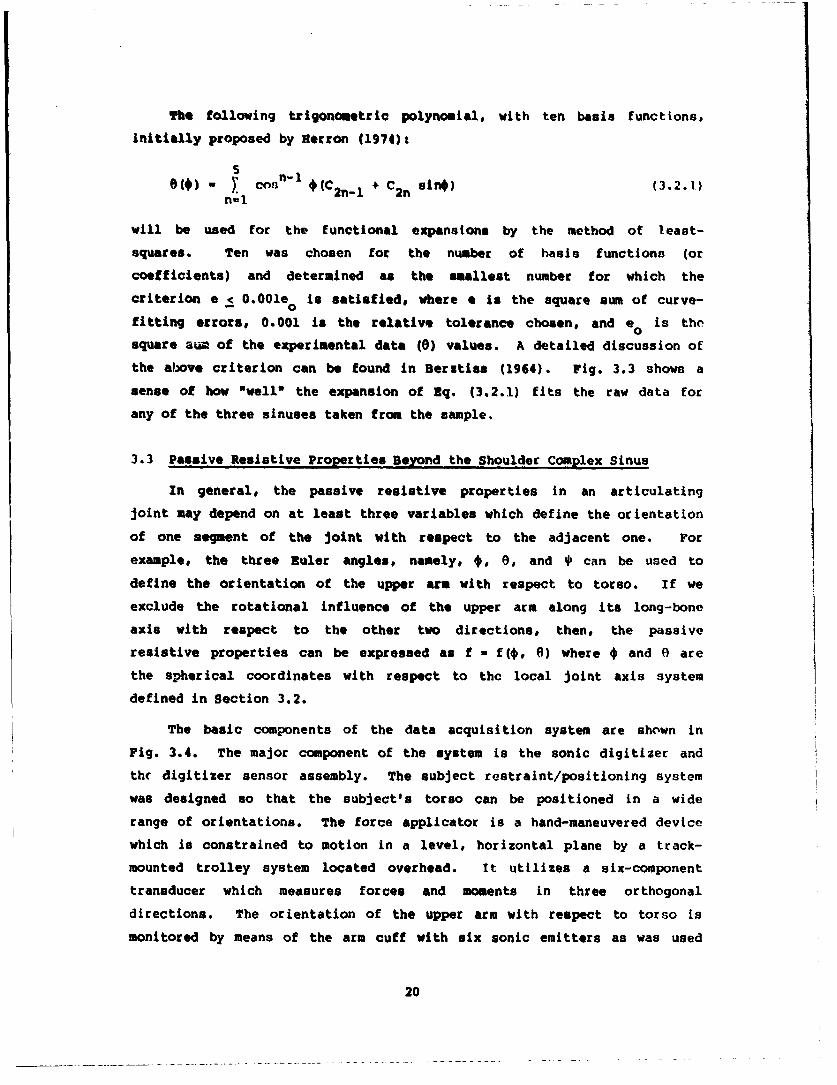
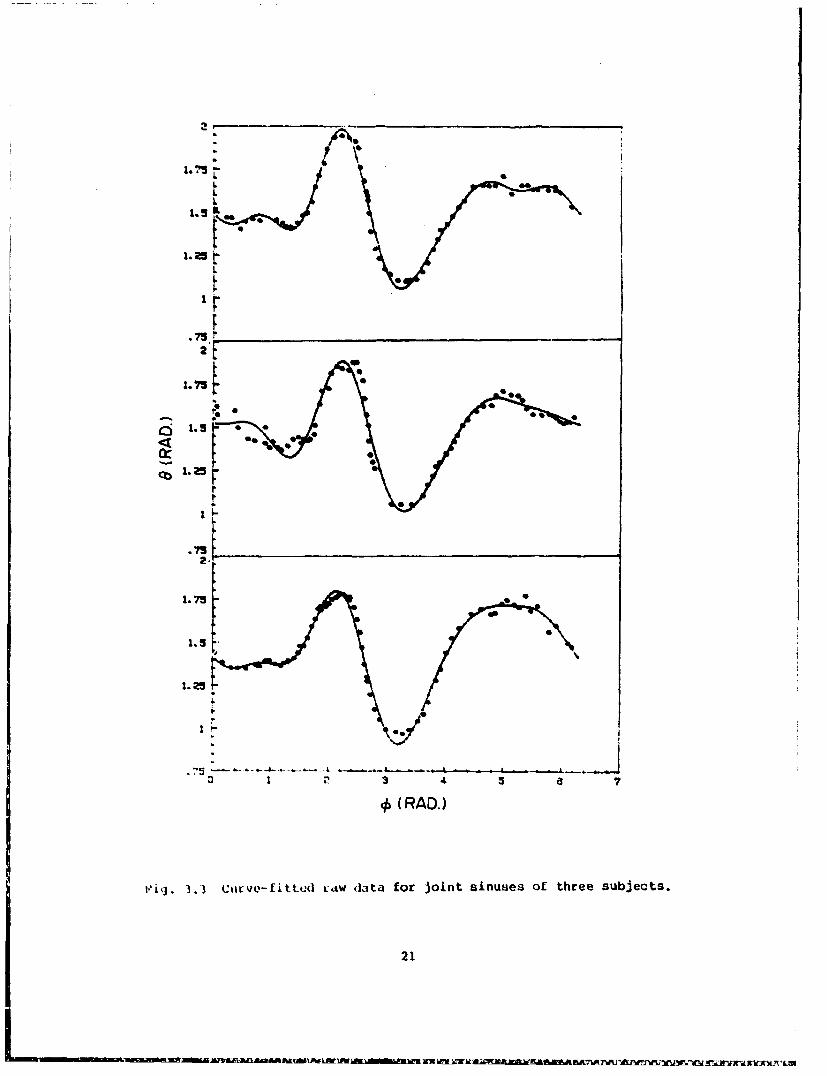
The following trigonometric polynomial, with ten basis functions,

Initially proposed by Herron (1974):

0 -) coo #(C 2 1 + C2 s4) (3.2.1)n-2

will be used for the functional expansions by the method of least-

squares. Ten was chosen for the number of basis functions (or

coefficients) and determined as the smallest number for which the

criterion e < 0.001e° is satisfied, where e is the square sum of curve-

fitting errors, 0.001 is the relative tolerance chosen, and e is the

square sum of the experimental data (r) values. A detailed discussion of

the above criterion can be found in Berstiss (1964). Fig. 3.3 shows a

sense of how "well* the expansion of Eq. (3.2.1) fits the raw data for

any of the three sinuses taken from the sample.

3.3 Passive Resistive Properties Beyond the Shoulder Complex Sinus

In general, the passive resistive properties in an articulating

joint may depend on at least three variables which define the orientation

of one segment of the joint with respect to the adjacent one. For

example, the three Ruler angles, namely, *, 0, and * can be used to

define the orientation of the upper arm with respect to torso. If we

exclude the rotational influence of the upper arm along its long-bone

axis with respect to the other two directions, then, the passive

resistive properties can be expressed as f - f(*, 8) where * and 0 are

the spherical coordinates with respect to the local joint axis system

defined in Section 3.2.

The basic components of the data acquisition system are shown in

Fig. 3.4. The major component of the system is the sonic digitizer and

thr digitizer sensor assembly. The subject restraint/positioning system

was designed so that the subject's torso can be positioned in a wide

range of orientations. The force applicator is a hand-maneuvered device

which is constrained to motion in a level, horizontal plane by a track-

mounted trolley system located overhead. It utilizes a six-component

transducer which measures forces and moments in three orthogonal

directions. The orientation of the upper arm with respect to torso is

monitored by means of the arm cuff with six sonic emitters as was used

20

tI.

L

Zr

1.75 •

.5

.713

1.5J

S(RAD.)

I"gj. 3.) Cturv.-fitted kLdw data for joint sinuues of three subjects.

21

IZ

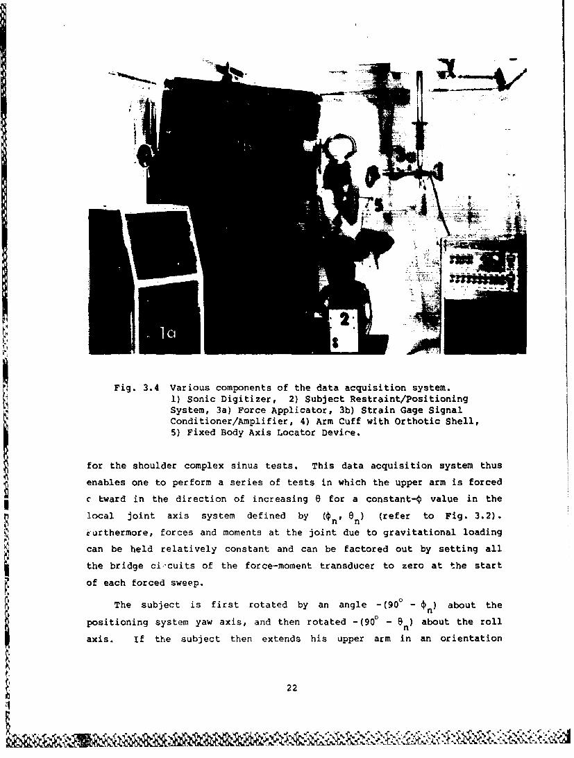
IIFig. 3.4 Various components of the data acquisition system.

1) Sonic Digitizer, 2) Subject Restraint/PositioningSystem, 3a) Force Applicator, 3b) Strain Gage Signal

Conditioner/Amplifier, 4) Arm Cuff with Orthotic Shell,5) Fixed Body Axis Locator Device.

for the shoulder complex sinus tests. This data acquisition system thus

enables one to perform a series of tests in which the upper arm is forced

c tward in the direction of increasing 6 for a constant-4 value in the

local joint axis system defined by (n' 1 ) (refer to Fig. 3.2).

eurthermore, forces and moments at the joint due to gravitational loading

can be held relatively constant and can be factored out by setting allthe bridge ci.-cuits of the force-moment transducer to zero at the startof each forced sweep.

The subject is first rotated by an angle -(90 - 'n) about the

positioning system yaw axis, and then rotated -( 900 - 0 ) about the roll

axis. If the subject then extends his upper arm in an orientation

22

parallel to the pitch axis of the positioning system, his humeral

longitudinal axis will be at (# n I ) with respect to the torso fixed body

axis system. The force applicator is then positioned vertically at the

samae level as the subject's upper arm, and the front of the force

transducer is strapped to the subject's arm near the elbow joint. The

subject is then asked to move his arm to its maximal position in the

constrained plane of motion of the force applicator. The arm is "backed-

off" from this position, and this then is the starting location of the

forced sweep. The subject's upper arm is then abducted or adducted in a

quasi-static manner until the subject experiences discomfort or the upper

arm can no longer be displaced (i.e.,adduction into the torso occurs).

The forced angular velocity, which is the same as the circumscription

"speed in obtaining the shoulder complex sinus described in Section 3.2,

is set at an average of 6I of arc/sec for these tests. During the entire

course of each test, the subject is instructed to let his arm hang limply

and not to actively (muscularly) resist the motion of the test. The

bridge circuits of the force-moment transducer are all set to zero at the

start of each test, so that the recorded values during the sweep are

departures from this "neutral" force orientation, or stating it in a

different manner, they are the passive resistive force values.

With respect to the joint axis system, these forced sweeps take

place in a direction of increasing 0, and at an approximately constant-4p

value. By then rotating the positioning system dDout its pitch axis, a

3eries of constant-ý sweeps are obtained. Each time, the force

applicator is vertically positioned at the proper level with the humeral

long]itudinal axis in a level horizontal plane. In this way the tests are

performed as four sub-series with each sub-series discernible by its own

oxperimental set-up configuration. The groupings consist of constant-€

:,w.'lp: In: 1) the upper-rear quadrant (00, * < 900), 2) the lower-rear

lIqadi~int (900 - 1800), 3) lower-front quadrant (1800 . < 2700) and

4) tfl, upper-front jua~drant (270'0 3600)

The ,•tik obtained according to the procedure outlined above were

analyzed an follows. First, the force and moment vectors obtained from

the force applicator ilat.a were used to calculate a total moment vector

with respect to the ln:.tantaiieous joint center which is chosen to be the

glcnohumeral joint center location. Next, a moment arm vector was

cdl(:ilated from the centor of the best-fitted sphere (described in

23

Nr

Section 3.2) to the point of force application. Next, the intersection

of this vector with a sphere of radius equal to one meter was selected an

a Onormalized' point of force application. The total moment vector wan.

then resolved into components along the moment arm i, perpendicular to

the moment arm vector. The component along the pon|tion vector (moment

arm vector) was then discarded, since it does not serve to restore the

moving segment to an orientation within the voluntary shoulder complex

sinus. From the remaining moment component and the normalized position

vector the resistive force vector was then calculated. Since the moment

arm is normalized to one meter, the magnitude of the resistive force

vector is the same as that of the resistive moment vector. we shall

refer to this magnitude as the passive resistive force (moment) property.

Note that this force vector is always tangent to the surface of the

selected normal sphere. Fig. 3.5 depicts the vectors and coordinates

specified in the analysis.

MOMENT VECTOR ' MOMENT VECTOR

""T lT CENTER OF THE

I TBEST FITTEDJOINT CENTER SPHERE

lob

ACTUAL POINT OF ZtbFORCE APPLICATION

ACTUAL APPLIED FORCE

CALCULATED RESTORING NORMALIZED" POINT OFFORCE FORCE APPLICATION

Fig. 3.5 Illustration of the vector quantities used in the

calculation of resistive force values.

24

Finally, to consolidate the vast amount of passive reasistive force

(moment) data and to facilite'"e the statistical analysis, the functional

expansion f(4. 8) must be c. .ablinbeds a variety of basis functions has

been investigate4 by utilizing the MM (General Linear Nodel) progrm of

the SAS (Statistical Analysis System) computer package (SAS User's Guide,

1912) of the Instruction and Research computer Center at The Ohio State

University. It wans found that the functional expansion

f(4, 8) a (C¢ + C2 cO4 + C3 rIini)0 + (C4cona # cs0°osint+ C6.sin 2 )e 2 + (C*co. 3* +coa5il*

+ Cgcosa$sn 2 * + C1 0 sin 34)0 3 (3.3.1)

provides the best fit. Ten was used for the number of basis functions

(or coefficients) and determined as the smallest number for which the

following criterion chosen

R2 - I - SMA . > 901 (3.3.2)

is satisfied, where

R2 (0 < R2 < 1) which is called the coefficient of multiple

determination and measures the proportionate reduction of total variation

in f associated with the use of the set of (%, 0) independent variables.

SSE is the error (residual) num of squares or

nS )Y t(r4I f ) - zi(4l, 0l)I2 and

55110 is- the total qum (4[ ý.tuarce. or

n -);) IZl(1. Oi) _ 2, where

n total number of experimental force (moment) daita points collected,

z• l l4 i) H -) the experimental force (moment) value collected at the ith

point (+j. 0 ) and

n I"- n Y ' (+ l it

i2 5

2'.

A detailed discussion of the R2 and relates r,•irv-sitm analysis can ho

found in Neter, et al. (193g).

Since 0(0 > 0) measures how fat the upper arm depaits from Lhit

a-axis of the local joint axis system, and # goes from 0 to 2w, we can

treat 0 &a the radial coordinate and # as the angular coordinate in the

polar caoidinate system (0, #). The pole is then the a-axis of the local

joint axis system . Therefore, it we introduce the following coordinate

transformation

p - $c00q - Osit* (3.1..1)

then (p, q' can be rearded as the corresponding rectangular coordinate

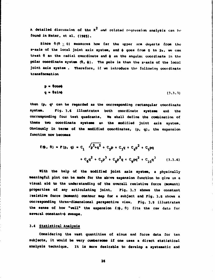
system. Fig. 3.6 illustrates both coordinate systems and the

corresponding four test quadrants. We shall define the combination of

these two coordinate systm an the modified joint axis system.

Obviously in term of the modified coordinates, (p, q), the expansion

function now becomes

f4* B) a F(p, q) - C1 /p2*q2 , p + C ÷ CCp2 + C pq

+ C6 q2 + C7 p3 + C 8plq 4 C9pq 2 + C10q3 13.3.4)

With the help of the modified Joint axis system, a physically

meaningful plot can be made for the above expansion function to give us a

visual aid to the understanding of the overall resistive force (moment)

properties of any articulating joint. Fig. 3.7 shows the constant

:esistive force (moaent) contour map for a subject and Fig. 3.8 shows a

corresponding three-dimensional perspective view. Fig. 3.9 illustrates

the sense of how *well* the expansion f(#, 0) fits the raw data for

several constant-4 sweeps.

3.4 Statistical Analysis

Considering the vast quantities of sinus and force data for ten

subjects, it would be very cumbersome if one uses a direct statistical

analysis technique. It is more desirable to develop a systematic and

26

QUAUNmT

((3rw/2c2,)

Fig. 3.6 The modified joint axls system and the correspondingfour test quadcants.

easily manageable approach to deal with the extensive data. Therefore,

Eqs. (3.2.1) and (3.3.1) will be utilized in an appropriate manner to

seek for a sample mean, sample varlance, and the confidence intervals for

the population mean and variance. In this section we shall derive the

method in a general sense.N

Let f(l) = • Ci gi (A) be a functional expansion (by the method ofi-1

least squarvas in this stuly) for the experimental measurenent of a"-0.certain quartity f having n independent variables, i.e., x a (x 1 , x 2 , x3 ,

0... xn), where {gij() Ii - 1. 2, 3. .... N) Is a set of mutually

independent basis functions, (Ci ii - 1, 2# 3 ... , NM) is the

27

(-2.5,2.5)(2525)

(-2.5,-2.5) (2.5, -2.5)

Fig. 3.7 Constant resiltive force (moment), in Newtons (Newton-Meters)# contour sap for a subject in the modified jointaxis system, in radians.

corresponding set of independent expansion coefficients, and H is thenumber of basis functions or coefficients. Consider now the statisticsof the quantity f for a chosen population from which we have a randomample of alse N. Then, obviously, the coefficients, Ci, becomestatistically independent random variables, and the non-random basisfunctions become statistically constant. Furthermore, f is now a linearcombination of random variables, and, so, is itself a random variable.

From probability theory, for each x, the population mean, p f(x), is

C() - 0[f(.)] . [ Ci )i-1

N 4.= gi(x) a[Ci] gi(W) itc (3.4.1)

28

(2512.5 (2.5,2.5)

(-2.59-2.5 1 I' (2 "..51-2.5)

Fig. 3.8 Perspective view of Fig. 3.7.

and the population variance, af(X)D is

2M

a f .X VAR[f(X)] - VAR[ C i gi W)i-i

N"2"jgilx) VAR[CC]1-1

a X gi() Y2 (3.4.2)

29

Z% - 2 4

l-

Z LIJZW

z t.

0"" 12

L4)W

z_D00•IO-

9U)

-12 . . . . . . . ...

0 .44 .06 1.32 1.76 2.2

8 (RAD.)

Fig. 3.9 Raw data and fitted curves drawn from f(o, e) forvarious constant-# sweeps for the subject mentioned inFig. 3.7.

where we have utilized

COV[C., Cj] - 0 for all 1 < i < J < I (3.4.3)

since all the coefficients are mutually independent. Note that in Eq.

(3.4.1) the operator X stands for the mathematical expectation and in Eq.

(3.4.2) the operator VAR for the variance. Therefore, if we know the

30

2population meant, IA and the population variances, a , for all the Kci ci

coefficLente, we can evaluate the population mean and variance for f(x).

Sample Meant i(x). and Sample Variance, S

Sinc* the population means and variances of the coeffic-ents can

rarely be obtained, we seek for statistical estimates, namely, the sample2means, Ci, and sample variances, S ci, from the given random sample of

size N. From statistical theory, an estimate for lic is

C N (Clo (3.4.4)i N Jul.i

where (C 1) stands for the ith coefficient of the Jth sample outcome, and

an unbiased estimate for 2 isci

S2 { j (C ) 2 1 [i (Ci) } (3.4.5)

Thus, an estimate for p f(x) from Eq. (3.4.1) is

(X ia' (3.4.6)

and an unbiased estimate for Of(x) from Eq. (3.4.2) is

s1i Sc (3.4.7)

Confidence Interval for .f() - tJf(X)

From statistical theory, the random variable (*)/

has a t-distribution with N-1 degrees of freedom, regardless of the

parameter values p (x) and Gf(X). Therefore, the confidence interval of

U (x) can be obtained by.. 4.

Pr (I < <() < - (3.4.8)- sf ()/ -IT

where Pr is the probability, y is the confidence level to be chosen, and

31

t•( >) is the solution of the equationY

iN.1 (P) dz - (3.4.9)

where ti.lis the probability density function of the t-distribution with

N-1 degrees of freedom. Rearranging the inequalities, we obtain the

confidence interval for uf(x), at the confidence level y,

OM. Wx - < V x) < lx + f (3.4.10)

Confidence interval for for(N-l) Sf(x)

The fact that the random variable 2 4 has a X2 -distributionof (x)

with N-1 degrees of freedom enables us to have

24

Y Yf(x)

where aY is the solution of the equation

2 (x)dz - 1 (3.4.12)

and B. is the solution of the equation

22

2N_1 (Wd - ,- (3.4,.13)

where X 2 is the probability density £anction of the x -distribution

with N-1 degrees of freedom. Rearranging the inequalities, we obtain the

confidence interval for O2(x), at the confidence level y,f

(N-1) 2 (N-1I) Sf(x)<GH '1 f (3.4.14)

cow f~(x) < 0

Y Y

3.5 Coordinate Transformations AmnzOg the Fixed Body, Individual Joint

and Mean Joint Axis Systems

Since we shall utilize the functional expansion forms, Eqs. (3.2.1)

and (3.3.1), to perform statistical analysis for the shoulder complex

32

sinuses and passive resistive properties beyond them, appropriate

coordinate systems should be consistently used for the purposes of

statistically comparing the coefficients of the data sets for ten

subjects. In representing the joint property data in functional

expansion form, different coordinate systems used will result in

different coefficients although the same basis functions are used.

Therefore, it is necessary to perform coordinate transformations for the

spherical angles, * and B, among the fixed body, individual local joint

and mean joint axis systems.

The local joint axis system, as bhown in Fig. 3.10 is uniquely

xit

y-." I I /

fb

fb 1 0

Fig. 3.10 Joint axis system as obtained by two successiverotations, first about the zfb-axis and then about

the intermediate (primed) y'-axis from the fixedbody axis system.

obtained in this study by first rotating the fixed body axis system by anangle *n about the zfb-axis and then rotating the intermediate (primed)

axis system by an angle n about the y'-axis. The mean joint axis system

is obtained in a similar manner with (n' On ) replaced by (m, ema)"

Since the joint sinus with spherical coordinates (ý, e) implies a unit

vector with rectangular coordinates (sinO coso, sinO si•, coae), the

Qoordinate transformation from (ýf, Gf), relative to the fixed body

33

axis system, to (t Oj) relative to the joint axis system, can be

obtained in the following manner:

$in[uCoisnOf coost [X

sine* id$in Njt/fb sinef abr]f 5

oe ij t % onef (3.5)jt

cose n 0 -inon ro n 1iowhere Vjt/fb 0 1 0 -s1* n Coon 0

nosin 0 coasen 00 1Loson cs0e n con saisn -sinen

"n -sn n COO n 0

sinOn Coon nsion sin cosO ni

is the transformation matrix defining the joint axis system relative tothe fixed body axis system, and x, y# a can be numerically calculated

with (*n, on) and the joint sinus (Cf, Of) specified. Comparing the left

and right hand sides of Eq. (3.5.1), we have

- tan-1 X and.x

e Cos-1 X (3.5.2)

The coordinate transformation from (*f, ef) to ( e * 9 ), where mjMj mj

stands for the mean joint axis system, can be obtained in the same way as

above with (* 1 9 ) replaced by ( , 1 0) so that the transformationn n m m

matrix defining the mean joint axis system relative to the fixed body

axis system now becomes

coae, coC m cosem mio m -sine

"Mjf " -sis, cos4. omJ/fb inr, a mlm

sinem cosm sinem aios coso9

34

It the joint sinus is given relative to the individual local joint

axis system, then the spherical coordinate transformation from (,4e O1)

to (4 j, eOJ can be achieved by noting that

sinO~ COO* sine1 COj

sinS U1 sin., mj * 4 J/fb Ltb/jt aminej s ir* Jcoenj J L comej j

LB ]1 (3.5.3)

-1 Twhere Lfb/jt " Njt/fb Jt/fb sinca jt/fb is a proper orthogonalmatrix, i.e.,

NTN jt/fb Nt/fb (3.5.4)

and X, Y, 2 can be numerically calculated with (% *m). (*n' *0 n) and the

joint sinus (it, 0 ) specified. Comparing the left and right hand sides

of Eq. (3.5.3), we have

-1Y

ýsJ = tan i and

e = COS -Z . (3.5.5)

3.6 Statistical Data Base for the Biomechanical Properties of the Human

Shoulder Complex

Since each subject has an individual local joint axis systemspecified by (n1 0) in statistically comparing the functional

expansion coefficients of the joint property data, two different sets of

sample means and sample variances can be envisioned and obtained from

different points of view:

1. Subject-Based Mean and Variance

Here, we consider each individual local joint axis system, defined

35

by (#no On)# as an Index attributable to the individual anatomical

variations in overall joint articulating structure as well as

muscle/ligament orientations, and subjective kinematic behavioral

variations in the circumscription mannerism. Then, not to be biased,

each individual Joint sinus and the resistive force (moment) data should

be described by (oil 04) with respect to the joint axis system of each

subject, namely,

0J a e%(* ) for the shoulder complex sinus, and

F 0 F(*j* ej) for the resistive force (moment).

The f unctional expansion coefficients obtained from these data are

called subiect-based coefficients. Furthermore, the population/sample

means and variances obtained from the subject-based coefficients will be

called subject-based population/sample means and variances, respectively.

Obviously, from a statistical point of view, the most appropriate axis

system for the subject-based population/sample means and variances is the

population/sample mean joint axis system.

2. * pce-Based Mean and Variance

In this case, the shoulder complex sinuses and the resistive force

(moment) data are described by (* d e, ) with respect to a common mean

joint axis system for all subjects, namely,

em - Omj) for the shoulder complex sinus, and

F a F(O , 0 ) for the resistive force (moment).mj isi

The functional expansion coefficients obtained from these data are

now called space-based coefficients. In addition, the population/sample

means and variances obtained from the space-based coefficients will be

called space-based r ,ilation/sample means and variances, respectively.

Maximum Voluntary Shoulder Complex Sinus

Table 3.2 lists L. ten subject-based coefficients of the shoulder

complex sinuses for *' ten subjects. Table 3.3 lists the corresponding

36

I- r4 0 P-1 f- %D P- s-4 1- 40 %DIl. qw wa IA P% 0 %D n 0 40 to '0 0 In m% PI 0o %D %D 0co

o N ' N V% 4 %D 0 at C% N P 0- 0 %D co go P. ma 0- CD4

F- S S 4 %D t- en co S

%D o% rI I I a% N I4 I IN w N- - - 1" - - -A a

4N N o- %a N at P. 0 m . 0% N%D N 0 P r4 MD N %D %D 4' p40

C; C; C; N; C; C; C; IA 4' 0

40 N -N n qv "r N In N% %D4% 04) ca 4 4 0 r4 %D "I N e CD

t2 I4 qv 4I I% I in I- Ir Ip44

%0 'a 04 t' p n4ro 0 o (a4 a m% at tA N0. 4 a

U C (1N m 4 4' al ND p4 N in 0

* In %b 4 N 4 en asua at an m 'a en a en a00

or m f" V- %_c_%_ýn I*i

'a P. N' Nn a0 04 (4n M .pA 0m %4 %D P.(4P In I'n cc Nn a

P. 4 at r4 m a -4% u (4 C41 t- IA'In ( r41 N' qn on % LN an P. am cA

V) mA ar 1 Na C% N r N% P. N %Dm co a, 4%a 0r at% %0 f' ( In 0i0044 Co w4 in 0% 4 N 'a pa 0 in 'a

0) w4 LA C4' P. % to% 0% 00 4 0% N4r4 en mS S~ N 4 40

0 0- 0o fn N'N P a a(%%D 'a 'a C4 .4v IA 0 N D4 00 ' 4

NA 40 94 N4 P. M4 fn N4 N P. P.N

IA in p %0 N4 r4 m In A P 0040 CD p4 N a at (% p 41 N' N- t an

m- w m 0 M M 40 5 tA Sq CD.0a a4 a o a al a% a0 N a a a% a

:I U I4 ID P 4 rI 0

N4 4' " 0 N P.1 ' 0% 'a No 'a 'at' (4% 0% a% ' % Na co V4 I IA r4N N en 0Iqv t N Go Ch 0 0-I441'

H' o% co NA N P. P. in m4 m 4 0n P4 Wo N' (% 4' in in aND

P4 I I II I 4 .4 c I

IV -- - - - - ------ ------ -----o ~ ~~~~~~ 'a P ' a 4 aP 4

U~~~ ~ ~~~~ 'a S . ' 0% 4 4'a 04

4' P. (4% 4 0 . p4 P. P '37

'A CN 0 M~' P4 40 C4 n N 4h M -orIn n Mj n4~ to a

C ~ ~ ~ 1 0

a I. V

41 w 4 en4 t 0% N0 f-4 0 40%~4 Woli I- % N 4 N a0%r~ 40 6M % a N P4 0% (v 4 liU v a N N M4 r. N In %D S 4

M N at 0A 0 0 0 0 0 0

v4 %a Nn lob 0% 'a S a N 0 4'0to 0 04 f-4 0 % 04' 0 N

to N0 4n m n F4 In N n N,a t- in w% ' P P4 in a m 4' 0

ov u N a% li 4'o n N4 a 0- P4 n F4

0 N 0o N

%D. -t-- - a% SO -In - -mI0 P P1 6 4'Co n 0 4 in 6 0 N%u 04 64 ID .0% fnS n 0h IV InnuI N% An C" 0 % 0a 040 64 In qv1 0

in N t qv wtS nN % in Chin am %') i' n in ea n r4 ao %'

*4 0 0 mS in 5% M1 04 Nn 6 n 04o U 0% 0% 5% 'a4 t- 6 1 0 4 n04o1 N N1 P % ' % ' % S ' S

4- N cc co a N N a%C2C %-4 CO -

m% q% 0% 0 0 at 0 qv0 lvqn m 0% 4' 5% '0 5 r4' S C' Sn 0%avi 04 m4 0n Ch %4S0 n P1 5 464 ~ " 64 N 0 W46 ~ i 4 1 -

o ~ ~ C n rI Ib% CO wr4 m l % 0 n m% P1 0 Sn2 P'a~~. 04 Sn 64CD1 6 N P 40% In Sn In r1' % tn tN %N5

or-i 4' %' Go at 64l a ' N 0 00

.9-I -so

m 1 ' % N 0 P 0 ' 1 0S4- N 4' 4 0 0 N N '0 P10%0

O 'a 5% 0 0% S 64 4 0 ' 4''a38

ten space-based coefficients. These two tables also list the sample

means and vatiances for all ten coefficients. Fig. 3.11 ohmes the best

1.75

1.5

SUBJECT-BASED

1.25

SPACE-BASED

.75

0 I 2 3 4 5 6 7*(RAD.)

Fig. 3.11 Subject-based and space-based maximum voluntaryshoulder complex sinuses for the first subject

fitted curves for both space-based and subject-based sinuses for the

first subject who has the (4 On) "(570@37, 720.24) which depart then n

most irom the mean values (*.' On) (590.29, 79°.08). The swore the

individual joint axis system deviates from the mean joint axis system,

the bigger is the diffqrence between the space-based and the subject-

based sinuses.

Now let us apply the results obtained from the statistical analysis

developed in Section 3.4 to establish a statistical lata base for the

shoulder complex sinus. In this case, the functional expansion,

39

Eq. (3.2.1), has only one independent variable# Loop *

Ftom Eq. (3.4.6) one obtains the sample mean

1 0 o n -lfl1( ý2n-1 * 2, i*) 361

and from Eq. (3.4.7) the unbiased sample variance

81 (s) I oo (8Zn- + S C sini~ (3.6.2)

Fig. 3.12 displays the least-squares fitted data for the subject-based

sinuses of all, ten subjects. This figure. also shows curves for the

sample meamo I(#*) and those corresponding to 9(*) g S(0). Fig. 3.13

2.25

1.77

.............. ............ .

**....... .. .. ~ *.

.75

01 2 48 7

S(RADW

Fig. 3.12 Curve-fitted data for subject-based sinuses of allsubjects (dotted curves). Solid curves are forSand 9 + 8e'*

40

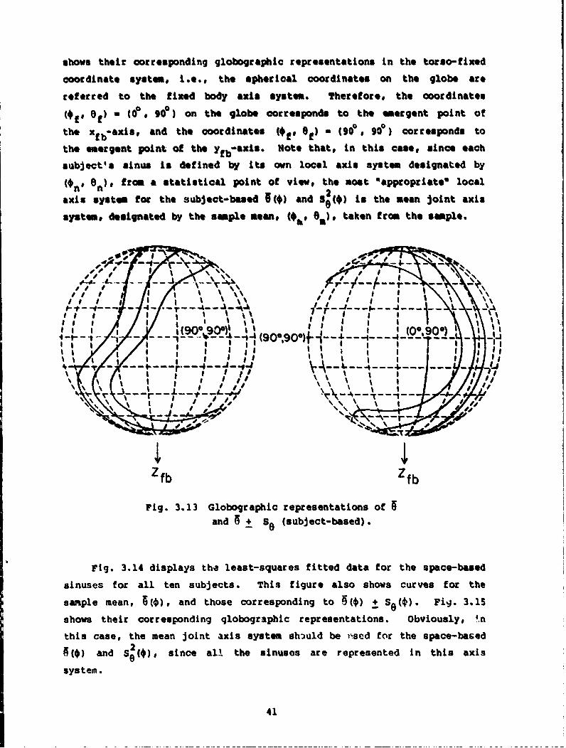
shows their corresponding globographic representations in the torso-fixed

coordinate system, i.e., the spherical coordinates on the globe are

referred to the fixed body axli system. Therefore, the coordinates

(#I. Of) - (0, 901) on the globe corresponds to the emergent point of

the xfb-axis, and the coordinates (%te Of) w (90P, 90e) corresponds to

the emergent point of the yfb-axie. Note that, in this case, since each

subject's sinus is defined by its own local axis system designated by

4n 0 8 ,n), from a statistical point of view, the most "appropriateO local

axis system for the subject-based 5(4) and S(0) Is the mean joint axis

systm, designated by the sample mean. #hA* ) taken from the sample.

A#!" N-SW-_J I

I I g oo) 00)"I 'I a i

'a a ' ,(9°e- 'Io'•,• ___

an 9 + 8 (sujet-asd)

sampl men 94, an ths corsodn ,"o "(• +" S q) - Fig-,-.15

4' ig --.---.---- ,1(9O O)H A ---._---__ ----...

i cae the i Is ," 't s

,,,

4, 441Zfb Zfb

Fig. 3.13 Globographic representations of

and • +_ SO (subject-based).

Fig. 3.14 displays the least-squares fitted data for the space-based

sinuses for all ten subjects. This figure also shows curves for the

sample mean, •(4), and those corresponding to 9(4) ± SO¢) Fi 3.15

shows their corresponding globographic representations. Obviously, 4.n

this case, the mean joint axis system should be ,•sed for the space-based

§(4) and 2•€) since e15. the sinuses are represented in this axis

systemn.

41

2.25 -

2.00

1.75

.50 .

1225 .•

,.ooo0.75

0.50 . . . ' . . . . . " . . - - - - - - • , - • , -0 I2 34567

S(RAD.)

Fig. 3.14 Least-squares fitted data (dotted lines) for thespace-based sinuses for all ten subj*cts. The middlesolid curve Is the space-based sample sean joint sinus,•(*). The upper and lower solid curves are

( + 8, (#) and 8(,) 98 e) • respectively.

For the purposes of comparison, rig. 3.16 displays the sample mean,

6W@, and those corresponding to 5(0) + S0 (*) for both apace based and

subject-based sinuses. It should be remarked that, while the space-based

and subject-based sinuses may differ significantly for an individual

subject, their sample means and# §(*) + S6(f)l may be indiscernible as

indicatIed in Fig. 3.16.

One of the most important ways of testing the ultimate overall

performance of the data acquisition system and efficacy of the associated

data analysis methodology is good repeatability of sample means and

sample standard deviations from different runs made on the same sample.

Fig. 3.17 displays the subject-based sample means# and B + S from three

42

different runs for all subjects. Rather good repeatability obviously

exists if one realizes that most of the deviations arise from the

variations during circumscription type of motion by the subjects.

4P

j I e' io

.I I II I I(o° o°

"\ ,J4 -(-724-0,900) A,

Zfb Zfb

Fig. 3.15 Globographic representations of •(€)and 64() + so (0) (space-based).

For the confidence level of 95%, utilizing Eq. (3.4.8), we obtain

from statistical table (Kreyszig, 1972) that,

Pr - 2.26 < __ /---,_-_ < 2.26 95% (3.6.3)

Rearranging the inequalities, we obtain

PrI , - 0.715 Se(t)1 <_ A() e < [6(•) + 0.715 Se(f)]} :F 95%(3.6.4)

In other words, we are 95% confident that the populati.)n mean Ve(0) is

within the interval [6(ý) - 0715S8 (@), O(@) + 0.715S (f)] at each value

of *.

Fig. 3.18 shows the confidence intervals for both the space-based

and subject-based population means for comparison. Fig. 3.19 displays

the globographic representation of the confidence interval for the

43

2 .1 t - - - '•

•+Se

1.8

< 1.5

+1 1.2

0.9

0 1 2 3 4 5 6 716 (RAD.)

Fig. 3.16 §(•) and +(*) + S (ý) for both space-based andsubject-based ainises. Note that the two 9 curvescoincide with each other in this figure.

subject-based population mean, U().

For the confidence interval of the population variance, from

Eq. (3.4.11), we have

9 92 I

Pr 2.70 < -21) < 19.02 -950 (3.6.5)

20 e

with 2.5% of probability on both tails of the x 2-distribution curve.

Rearranging the inequalities, we have

Pr 0.473 S2 2 < 3 2 M 95 (3.6.6)

44

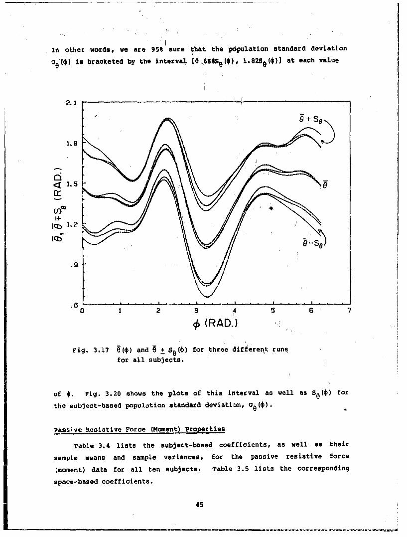
In other words, we are 95% sure that the population standard deviation

is bracketed by the interval 10.,688S 0(€), 1.82Se(€)) at each value

2.1 ~

1.8S

< , 1.5

1+I~1.2

.9"

0 1 2 3 4 5 6 7#(RAD.)

Fig. 3.17 O(€) and 6 + Se(f) for three different runs

for all subjects.

of F. Pig. 3.20 shows the plots of this interval as well as S (f) for

the subject-based population standard deviation, ae(0).

Passive Resistive Force (Moment) Properties

Table 3.4 lists the subject-based coefficients, as well as their

sample means and sample variances, for the passive resistive force

(moment) data for all ten subjects. Table 3.5 lists the corresponding

space-based coefficients.

45

2.1 -_ _ _ _ _ _ _

< 1.5

too 1.5

0.

0.9

f(RAD.)

Fig. 3.18 Confidence intervals (CI) for both the space-basedand subject-based population means.*

From Eq. (3.4.6) one obtains the sample mean

f(, )* C+ C2 OOt + a sit4)8 + (aCo 20

+Ccossiai4~ + d 6 sin2 6 7 (Cvos 3 + Ccoo2 sInf

+C 9cozosin 0 + C 10sin f)e (3-r7)

46

IT,. / ,, ,, I t • / # i l , \ \ .i i i I /! ' . t r f, t , mean,,t-+--, ----- -4 -- t, ----'-- -'.--'- -, -/ -

II I , I 1(9 ,9 1 I.,,ro,,.,,L • - - - -'• -. 'L IIL I.

i mean U..

and fro Eq.,v (3..7 th sapl variance0

f I; C 2 3 C 4I

Zfb Zfb

Slobographic representations for the sample mean, C ,Fi.3.9and the 95% Confidence Interval for the subject-based

population mean, "

and from E.q. (3.4.7) the sample variance

22 2 2 2 2 2 2 4 42

+ S cos sint + S i osn sin + (s ,COBC C C C

C8 9 C1 0

(3.6.8)

Note that, in this case, the functional expansion for the force (moment)

properties, i.e. Eq. (3.3.1), has two independent variables, ý and e.

Fig. 3.21 shown both the space-based and the subject-based sample

means tor the passive resistive force (moment) property in the form of a

constant contour map. Since the difference between these two contour

maps is imperceptible they are shown in two separate figures rather than

in a superimposed format.

47

2

1.5

<So

O .2 aSe56

I--4

.5

.• • 0.688 S9

0 1 2 #(RA 4 5 67(RAD.)

rig. 3.20 The 95% Confidence Interval (CI) for thepopulation standard deviation, 07 . Thesubject-based sample standard deliation,see Is also shown.

It should be mentioned that the force (moment) data were collected

beyond the maximum voluntary sinus up to the point, which will be

referred to as the maximum forced sinus, where the subject starts

experiencing discomfort or the upper arm can no longer be moved (i.e.

adduction into the torso occurs). The raw data for the maximal forced

sinus are curve fitted by the sae functional expansion used for the

maximal voluntary sinus. Table 3.6 lists the subject-based coefficients

as well as their sample means and sample variances for the ten subjects'

maximal forced sinuses. The statistical analysis procedure is also

applied to the maximum forced sinuses. Fig. 3.22, for comparison,

displays the space-based as well an the subject-based sample means for

the maximal forced sinuses. With the exception of the region 0 < $ < E,

48

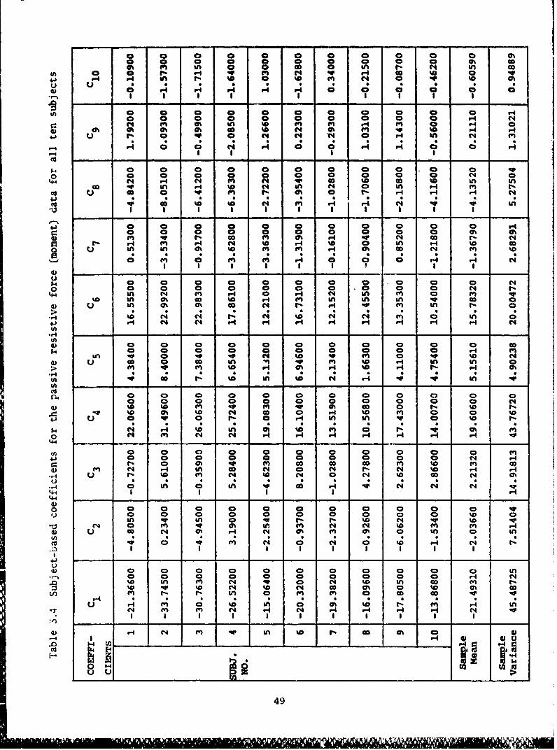
0 a a 0 0 0 0 a 0 0 ata I 0 0 0 4 0 In 0% con

4" n 0 0 co 0 in .4 4 &n co+j r- r- In f% %D 0 %D m C a op D

U 0r4 A - .4 4 ; c; ; a ; a; aa

* 1 01 @ 01 0 'a N 01 Q' 'a 0 H-9:~ a4 m a% In w en C" N- " 0

-, m m 0C 0% N2 ID C1 at en qw a-4I a I1 HI - - 00r

a 0 a a a a2 a0 a CD a vo a a a0 a a0 a 0 N 0

4 H4 N CD N 0r CD % 0 Go %Dn kn

0r r4 N 'a N A N 0 In HM3

o 0 0 0 3 .0 0 CD H H 0 N4

0 a a a 0 a ao a aq* r% O0 4'n 0m H- 4 N co I- N

r- H- ('" r N %D H- %D 0 In H1 %0 cc

o 0 IA A 0) 'a 0' a' Q CO 0 N0 0' 44

a C a a D 0 4 a a 4 H N%D an 0% c a 4 I" in 0 an qwC

In 0 0 -o - - - - - - - - - - - - - - - - - - - - - - -

>- %Z a4 a a A a A A a4 aý M;

o a 40 a a 0 a ) 0 a 0 4 a a Go3U) C 1-1 H2 0 H0 N CD V4 ')

'a 1* 0 0 qv Hr N ' %D IV Wi a " D4) coI 01 co n In "r Hn to H' kA k a

> m N0 f" % H H H H H H N%

W- - a;en

0)a a a a0 a a 0 a) a a a%a a an av a a a% ao a al %a t-%a at %D 4 cc a r4 %a mN0CD %

4- a0w 0 C- 0 IA I in Hn v A C1 %U') A 4') Wa H; 01 A 'a H: 3% H

.5- q N C4 q 5- S- r- r4 P-4

a a 0 a a 40 a a0 a C) a4- CD C a a a aD a aD a 0 q N4

r- cl 1 a a% R'ao O c omG

'a 'aU) M 044'i c 4 C r- N %V H'aw% fn N In In C 04 to'N

0 *0 0 0

fja 01 4' 0' 0 0 a 4)'a010 N4 H IV P in fn N C4 ND ma m H

d) 3% CD 0 N0 aC N a N0 'a a N40 Q a C) 0 C 0 H ý 4' N 0 NNw in I" N Hr 4 4 % n c n

oV -W a o 4 %a a1 ao a% 0 aD M oV) (n - a- LM 3 'a c" fn 'a) OD CDIV

04 m M N r4 N 01 i FCl 0 n

4 J4

U3UlI8 a a a a a i

a a a a a a a o a a 49

LWI ') N 4 a N aa3

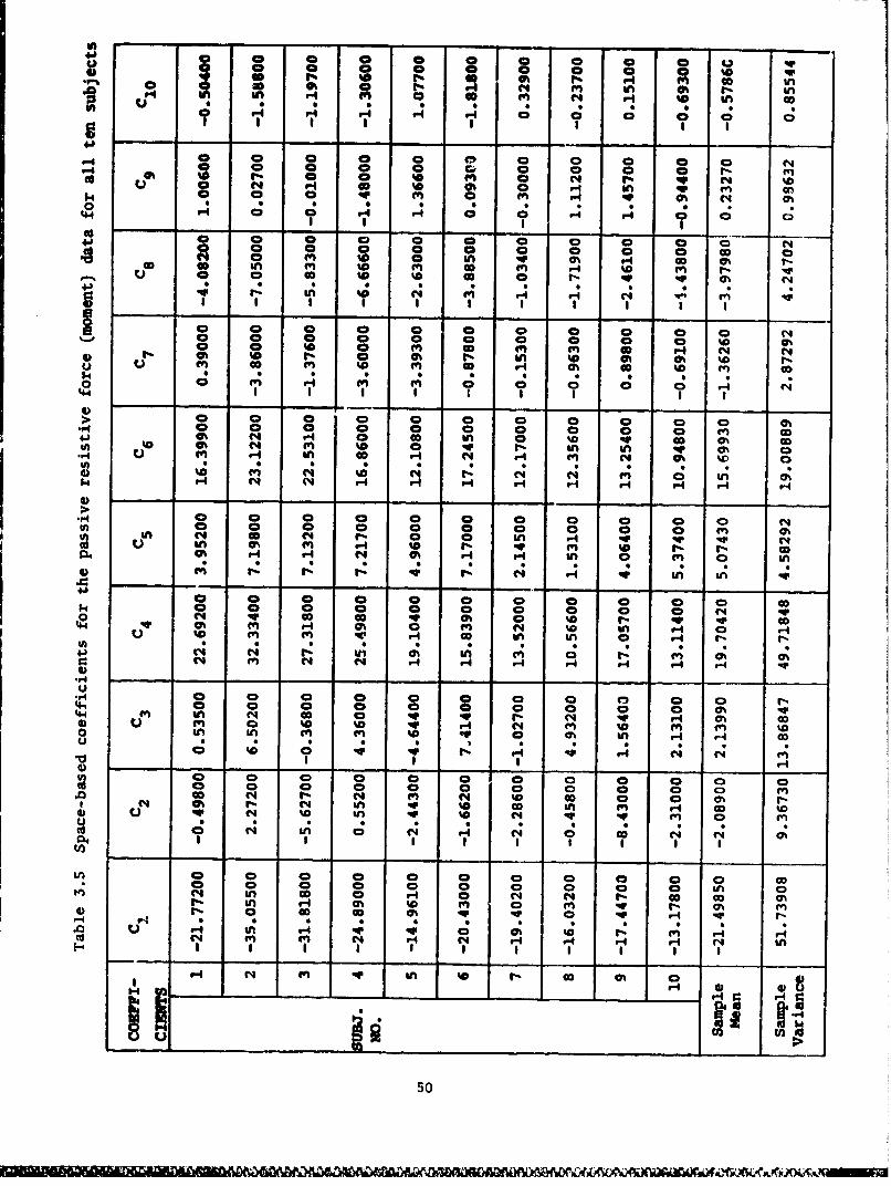
-R - -r- - - ' - - - to

0 0 0 0 0 0 a 0 0 0. C4a 0 0 0 0 0 0 0 40 to (q4" a t 04 Ch

N 0 m. w a in a r-o o 10 0n M %a M t 0 0 in~ IMlu 0 C2 -o %0 %D 40 0 1-I Vi

42 0 0 0 0 0 0 0 0 0N0 0 0 0 0 0 0 40 0 CD %D 0

>0 CO 0 a 0 a 0 0 8 40 CD at.r 0 Pt t 0 0f '9 0% 0 0 M% cc01 0% IN t4 0 t i 0 Pt 10 40 Pt ODUl % a Ch 04 to %0 0 av r. In In IV'"l It" UI an o C4 v-4 en 04 M %V 0

r-4 ~ ~ C4 ( 4" Il r -

0 Q 0 0 a a a a a 40 t 0 Pt 0 Pt Pt a en N

9 in 0%, fn 3%l to r- q% ui %o0% r t- CO

0 t 0 P o P 0 C at 0 to C Goo 0 Pt 40 0, a a 0 0 0 C4 q

44 0 w qa Ch 0 f'.9 40 0% 0010 Ch en 4 WM to a n C4 IWO in .l Cr-tn o

C4 N c4 w; u; N t fl0 40 0 Vt 0 0 Q 0 nt 01 at tr H H H

a a a a 0 a a a a a 0% qVIn a 4 a o 0 a e r a l a 4 qa a a h O

00~ 0% 4' IV tor I- r-4 to f-4 C4 0

'90 0 C) 0 0% a o 6- 9 m CDC31 0% Pt 0% 0 Pt N to 0 Utcc) N t- 44 rn Nt kD D a P 0% 1,,

C4 at a% a a a a in In r-4 c%

40 4nN 0 aD '9 C2 3% N .9 H 0 Gn C4 In OD to Ho . N C4 t- cc CID t

f0 in 0% %D en t0 a " q% Sn H fn0S ; 0 999to a4 9n en C %4 C H 4-4 H N &n

en 7 II r H

4 )-8--

o a a a a a a a a a so

a a a a a a a a

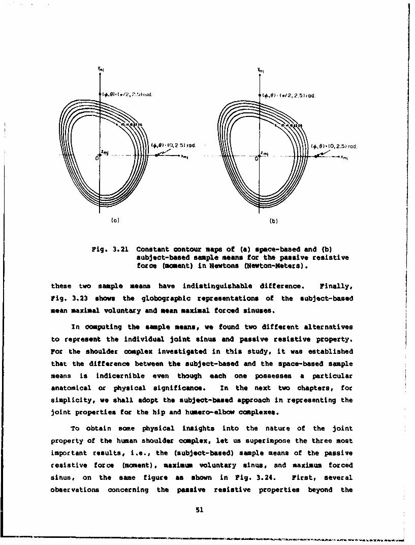
(0,2 5).rod. (4, •8e,) (O , 2.5) rod.

(a) (b)

Fig. 3.21 Constant contour maps of (a) space-based and (b)subject-based sample means for the passive resistiveforce (moment) in Newtons (Newton-etters).

these two sample means have indistinguishable difference. Finally,

Fig. 3.23 shown the globographic representations of the subject-based

mean maximal voluntary and mean maximal forced sinuses.

in computing the sample means, we found two different alternatives

to represent the individual joint sinus and passive resistive property.

For the shoulder complex investigated in this study, it was established

that the difference between the subject-based and the space-based sample

means is indicernible even though each one possesses a particular

anatomical or physical significance. In the next two chapters, for

simplicity, we shall adopt the subject-based approach in representing the

Joint properties for the hip and humero-elbow complexes.

To obtain some physical insights into the nature of the joint

property of the human shoulder complex, let us superimpose the three most

important results, i.e., the (subject-based) sample means of the passive

resistive force (moment), maximum voluntary sinus, and maximum forced

sinus, on the same figure as shown in Fig. 3.24. First, several

observations concerning the passive resistive properties beyond the

51

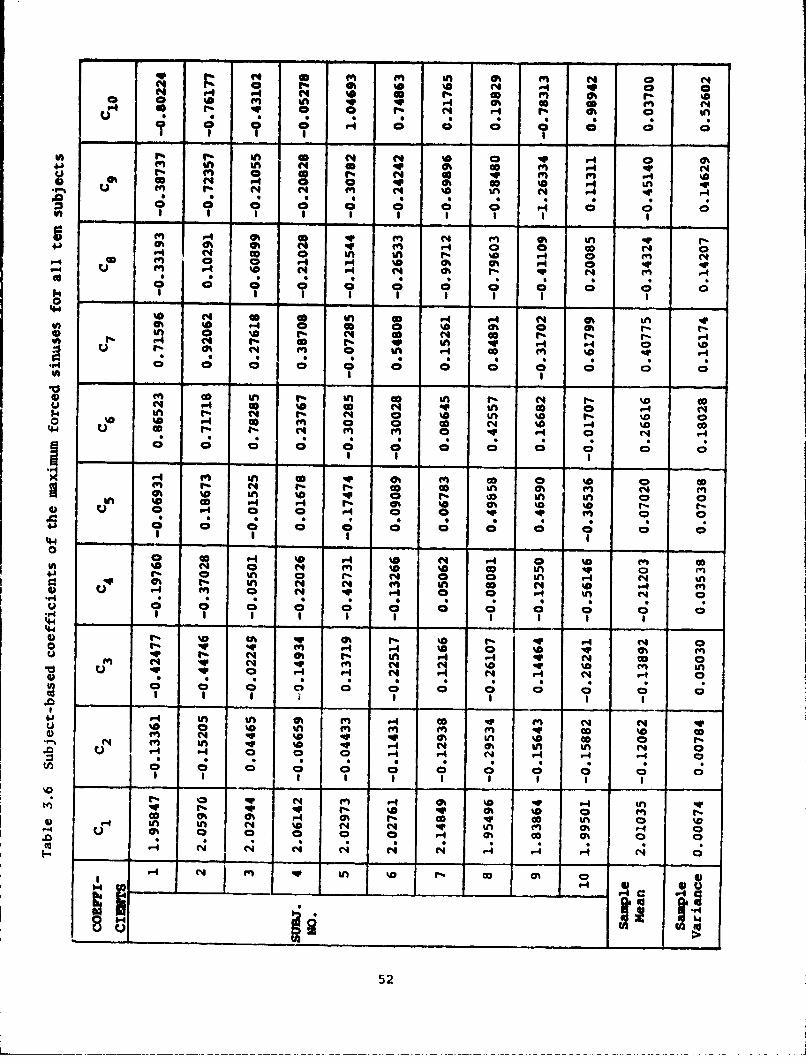
C4 N 0 aA 0N% r4 P4 is r- %D4a aa %D% M P4 ch co C

r4 X % N " % 0 0 kA

oi in 0 " 04 %D P4 0 0h

4-6 %n 10 P4 M a 0 4 "40 Ch C4 00 CO %D P499%~~ M % % N M

Ch Ch 0t N M9 0 co N % 0 ' 9I

cc m 0 4 P0 0a 0h 0n r 0 0 0- -- %-N P- r 0 N1

M~c "4 P4 0qv % A49vi at 0% -.4 V, w at at 0 0N""9f N A IA co 'a. "9 0M0 a t- r- in 'a r-4 9-4 %9 0Ul m C4 Aa N in N - co m% %D

0 -- -2 %D -w-% a w r4 0 IA 0 "o N9 Nco

H a in 0o qv 0 wa 0 04m %0 'a 9% No go Nin% %"

In 9% co N M % A "9 0'a4"9 a V a a2

P4 %D~ P4 %DIA 0 I N 9% MD o0 "9 0 % N 4 I 0 0 -.4 9%NCh NA cl m co N4 a0 InI 0 %L7 'a 'a %n 0C4 ' 9'

0 fn P4 w% Nat " N

M 9% N N% in00 IA 0

IA 'a 0 w %9 "9 0% 0% %a w% 'a ' 0*0 lu V- P4 "4 9 a 0

co. -h o% r4 a - cc 4o t0 0- "9 'a N9 ' N v 9 0 'a 04at 0% Go 0%a 9 a I 9NI

N "9 M N 4 "9 a4 a 9C4aq aW in aD a, aw

I I I I I I 52

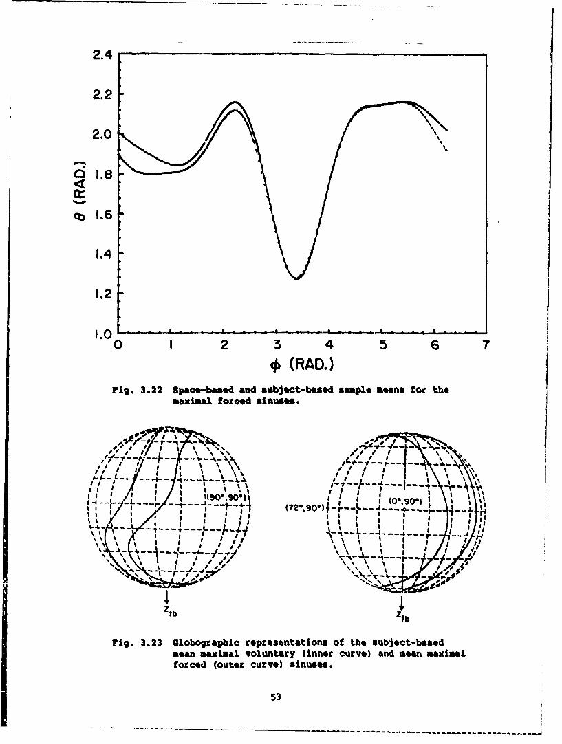
2 .4 ...

2.2

2.0

01.6

1.4

1,2

1.0 - -

0 I 2 3 4 5 6 7

4 (RAD.)

Fig. 3.22 Space-based and subject-based sample means for themaximal forced sinuses.

X .

I I

5 a *' I a,*.-4--L. iL'•a O¶0,,---•-a- --'-- --- t'---- a.9 .• . . . .. .I I - ii~1r, a- --- -- --

Nj NA

,Ip

Ztb Zfb

Fig. 3.23 Globographic representations of the subject-basedmean maximal voluntary (inner curve) and mean maximalforced (outer curve) sinuses.

53

-----------------------------------------/.n,

(-2.5, 2.5)1 '(2,5, 25~)

(-2.59 -25)-

isp

asonFig.h.4S~t-d surmise andn aopt tohue psin curentyeistivgfotrcgened tmontal-hman-body modlunays. ns(nerdse)

2.xma voutare shoulder complex sins least resilienti: h ora

quadrants (0 < < r) *in this region, more or less constant

54

%" ~ ~ '~

foace (moment) values [between 14 and 1.0 Newtons (Newton-

M4ters)] were observed to initiate discomfort.

3. The lover front portion (,w < I V) of the plot exhibits the

most resilient behavior due to adduction of the upVper arm into

the torso. no real disomfort was observed and the maximal

forced sinus in this region in based on the 9 values reached as

far as possible during the constant-* sweeps for the force

(moment) levels which were applied.

4. The upper front region (3v < 0 < 2w) exhibits an intermediate

(transitional) characteristic in terms of resilience. In this

region, discomfort initiates at the force (moment) level of

about 26 Newtons (Newton-Meters).

Second, the maximum voluntary and forced sinuses specify the

applicable domain of the passive resistive property. The resistive

forces (moments) below the maximal voluntary sinus are appreciably lower

in magnitude and thus can be neglected. Therefore, the maximal voluntary

sinus can be considered as the lower limit of the applicable range for

the expansion function f(•. 6). In fact, Fig. 3.9 shows that in the

neighborhood of the origin (pole), dashed curves indicate both lacking

good fit and being outside the applicable domain. In the strict sense.

the upper limit is the maximal forced sinus for the applicability

of H(ow e). However, the extrapolated values by 1(%, 0) beyond this

upper limit are most likely predictions and can be used up to the point

of impending injury for the simulation studies of multisegmented

mathematical models.

55

0.1% W6AU~A4A a.. R-f PU AMkRMýlk~A~M ABAM

4. BIONBCRIH CAL PROPI•MU8 or TUa mWum HIP COMPLAX

4.1 introduction

This chapter deals with the in-vivo blonechanical properties of the

human hip complex in the sitting position with the torso being fixed.

The data so obtained are suitable for simulating a seated pilot an well

as an occupant in a car.

The term *hip complex" refers to the combination.of the hip joint,

pelvis, lumbar spinet and their articulations. 11:ig. 4.1 shows the

principal bones and ligaments of the hip complex" Since the femoral

notion, while sitting with torso being fixed, is ,rmally accompanied by

lumbar flexion and pelvic tilting, it is more ari-*tpriate to use the

tern Ohip complex sinus,. rather than "hip Joint sinus,' to designate the

range of extreme allowable notion of the femur with respect to torso.

The human hip has been normally modeled as a three-degree-of-freedom ball

and socket joint by most researchers (Dempster, 1955; Johnston and Smidt,

19691 Chao et al., 19701 Lamoreuxt 1971), although in some cases it has

also been simplified by neglecting the axial rotation (Saunders et al.,

19531 Paul, 1965). In planar motion studies, it is even assumed as a

one-degree-of-freedom revolute (or hinge) Joint (Clayson et al., 19661

Beckett and Chang, 1968).

Functionally, unlike the shoulder which has sacrificed stability in

favor of mobility, the hip provides essential stability for support of

the body as well as a certain degree of mobility. Structurally, the

pelvis is more rigid than the rather freely movable scapula. The

interplay among the hip joint, pelvis, and lumbar spine is similar to

that between the shoulder joint (the glenohumeral joint) and the shoulder

girdle which includes the clavicle and the scapula. However, the

articulations of the sacroiliac joint and symphysis pubis provide much

less mobility than those of the shoulder girdle. Furthermore, the joint

capsule, the ligaments, and the muscles have reduced the freedom of the

hip joint whose bony structure permits almost as much mobility as is

found in the glenohumeral Joint. For example, hip hyperextension is

practically insignificant mainly due to the ligamentous check of the

iliofemoral (Y) ligament. Finally, it should be noted that hip flexion

is also dependent upon the amount of knee flexion due to the interaction

56

- - - - - -- - - - - - - - -.. . . . . . .. . . ..... ..

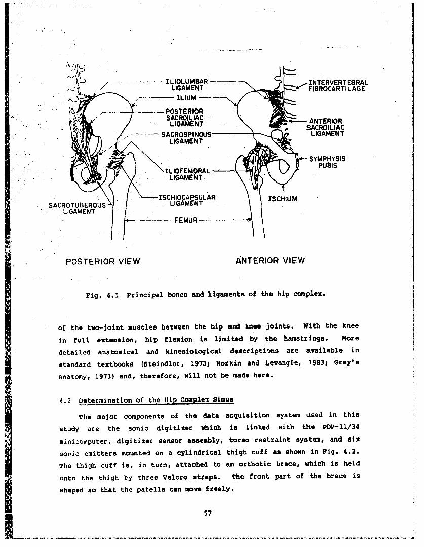
ILIOLUMBAR C .,INTERVERTEBRAL

LIGAMENT FIBROCARTILAGE

1< / ILIUM-

Q\" -. '" - POSTERIOR

LIGAMENT ANTERIORt• , • SACROILIAC

SACROSPINOUS LIGAMENTLIGAMENT

-- SYMPHYSIS,: ;. ..... :} • ., +L ; PUBIS

ILIOFEhMORALPUS

rSC HIOCAPSULAR SIUSACROTUBEROUSr LIGAMENT

LIGAMENT,FEMUR

POSTERIOR VIEW ANTERIOR VIEW

Fig. 4.1 Principal bones and ligaments of the hip complex.

of the two-joint muscles between the hip and knee joints. With the knee

in full extension, hip flexion is limited by the hamstrings. More

detailed anatomical and kinesiological descriptions are available in

standard textbooks (Steindler, 19731 Norkin and Levangie, 1983; Gray's

Anatomy, 1973) and, therefore, will not be made here.

4.2 Determination of the Hip Complex Sinus

The major components of the data acquisition system used in this

study are the sonic digitizer which is linked with the PDP-11/34

minicomputer, digitizer sensor assembly, torso restraint system, and six

sonic emitters mounted on a cylindrical thigh cuff as shown in Fig. 4.2.

The thigh cuff is, in turn, attached to an orthotic brace, which is held

onto the thigh by three Velcro straps. The front part of the brace is

shaped so that the patella can move freely.

57

Fig. 4.2 Major components of the data acquisitions system.1) Sbnic: Digitizer, 2) Digitizer Sensor Assembly,Torso Restraint System, 4) Thigh Cuff with SixSonic Emitters.

"The quantitative determination of the hip complex sinus involves thefollowing basic steps: (1) immobilizing the torso to be treated as the"fixed body and defining the fixed body axis system aa shown inFig. 3.2(a), (2) having the subject move the upper leg along the maximalvoluntary range of motion and monitor, with respect to the fixed bodyaxis system, the 3-D coordinatee of a distal point on the moving bodysegment; this point (to be referred to as the knee joint reference point)is selected as being on the mechanical axis of the femur at the level ofthe femoral lateral epicondyle, (3) fitting the knee joint referencepoint coordinates to a sphere using the least-squares method, thusestablishing a center for the best-fitted sphere and an idealized link

58

length. (adius of the sphere), (4) fitting a plane to the same knee joint

reference point coordinates to a sphere using the least-squares method;

the normal to this plane "(specified by the spherical coordinates n Oen nas shown in Fig. 4.3) establishes the. pole (z -axis) of a local joint

axis system with' respect tO which the hip complex sinus, designated by

the spherical coordinates (1, e) of the vector connecting the center of

the best--fitted sphere with the knee joint reference point, can be

expressed as a single-valued functional relationship, i.e., e 00).

• X

F ,eibhb

Fig. 4.3 and loientatoydeinte jint body (

.fb z, fb)adlclydfne on.xiY

Zjt ) axis systems.

59

., ',Q. " /

since only the knee joint reference Point is monitored in this

study# only the relationAshipe between this point and the six sonic

emitters on the thigh cuff need to be initialized. The calculations are

the same as those used for the origin of tle, longitudinal axis system

thoroughly diScUssed in Section 2.2. .However, since the knee joint

reference point is inaccessiblep two emitters are needed to interpolate

it as being located at the center. The eraitter positioning for this,

initialization jrocess Is schematically shown in Fig. 4.4.

Before the hip complex ainus test, the subject ,eas -instructed to

move his upper leg along its maximal voluntary rarige of. motion, in a

counterclockwise motion as viewed from the sensor assembly. He lrap, also

instructed to displace the upper leg' istally along its longitildinal axis..

as far as possible at all tiuiGi' whilc .,Jrcumscribing top hip complex

sinus. Preferred rotation of the upper leg about its longitudinel' axis

as well as preferred knee Ilexiot were left, up to the discretion of the,

subject in obtaining the maximal contour. Several sweeps of this type

were practiced before' data' were collected so, that the subject could

experiment with obtaining the largest possible range of motion. in order

to help maintain a constant rate of motion during data collection, a

.large clock with an easily visible second hand was placed in front of the

subject. The subject was instructed to imagine his upper leg as"',the

second hand, and to synchronize his hip complex sinus circumscription

.with the clock's 60 second sweep.

Table 4.1 lists the centers and radii of the best-fitted spheres. and

On' en) values of the best-fitted planes ,,for all ten subjects. With

respect to each individual local joint axis system, Figs. 4.5-4.7 show

the hip complex sinuses for three subjects and their corresponding least-

squares fitted functional expansions of Eq. (3.2.1). Figs. 4.8-4.10

display the corresponding globographic representations of these three

subjects' functional expansion sinuses with respect to the fixed body

axis system.

4.3 Determination of the Passive Resistive Properties

As is the case for the forced tests on the shoulder complex, it is

also desirable to perform a series of forced tests in which the upper leg

is forced outward in the direction of increasing 0 for a constant-ý value

60

.di

LATERAL VIEW ANTERIOR VIEW

Fig. 4.4 Emitter positioning for initialization process.

61

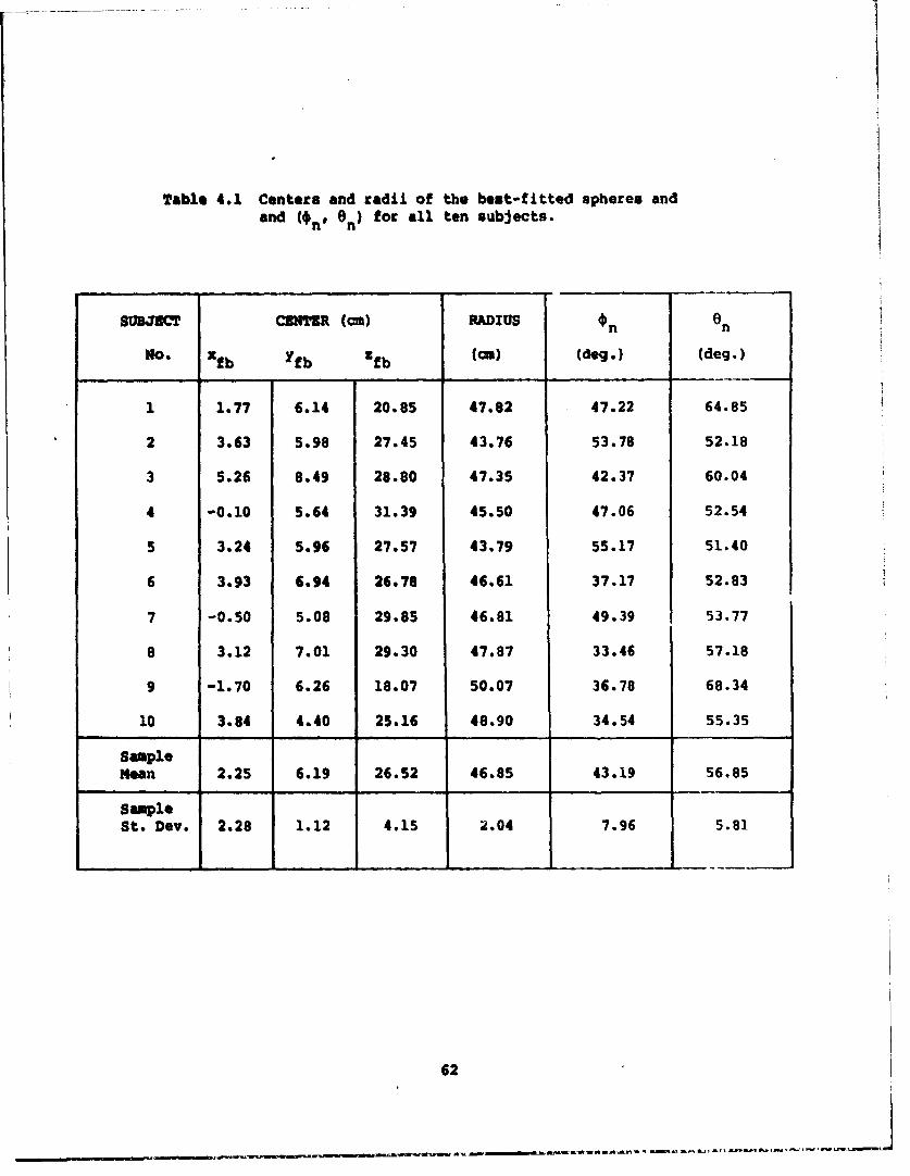
Table 4.1 Centers and radii of the best-fitted spheres andand (*n' On) for all ten subjects.

SUBJ3•CT CBEMR (cm) RADIUS 0nn

No. * fb Yfb Zfb (am) (deg.) (deg.)

1 1.77 6.14 20.85 47.82 47.22 64.85

2 3.63 5.98 27.45 43.76 53.78 52.18

3 5.26 8.49 28.80 47.35 42.37 60.04

4 -0.10 5.64 31.39 45.50 47.06 52.54

5 3.24 5.96 27.57 43.79 55.17 51.40

6 3.93 6.94 26.78 46.61 37.17 52.83

7 -0.50 5.08 29.85 46.81 49.39 53.77

8 3.12 7.01 29.30 47.87 33.46 57.18

9 -1.70 6.26 18.07 50.07 36.78 68.34

10 3.84 4.40 25.16 48.90 34.54 55.35

SampleMean 2.25 6.19 26.52 46.85 43.19 56.85

SampleSt. Dev. 2.28 1.12 4.15 2.04 7.96 5.81

62

rflt~~fl .,ar ..... - ---- --- -nalnl, l

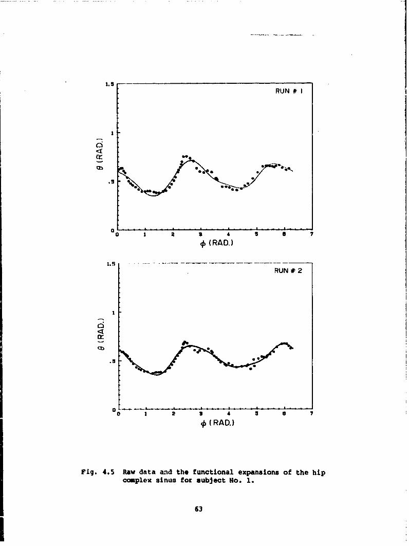
1.5'-

RUN # I

1

a:

- 0-

• 4 .. .. . .4. 54

RUN 2

0 *04e.A

a

0 1 2 3 4 5 7 7

S (RAD.)

Fig. 4.5 Raw data and the functional expansions of the hipcomplex sinus for subject No. 1.

63

RI

.rS~RUN # I

.S

.5

0a 24 - 4 £

0 1 2 3 4 5 a 7

S(RAW)

RUN # 2

CrQ

00

2 I I 4 3 !1

*(RAD.)

Fig. 4.6 Raw data and the functional expansion& of the hip

complex sinus for subject No. 2.

64

n ins~s~~atr ..3S .. tS~f fl~, ffl a, -

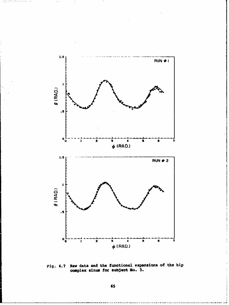
RUN #I

11

'5•

3 2 3 4 5 a ?

4, (RAD.)

RUN 2

.5

a a a 4 5 a 7

, (RAD.)

Fig. 4.7 Raw data and the functional expansions of the hip

caumplex sinus fot subject No. 3.

65

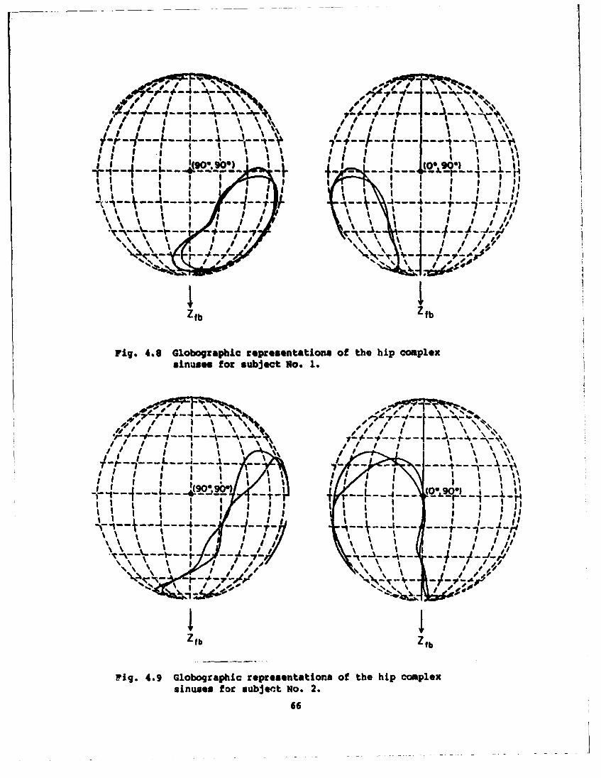
S, i ,, eo 4 .44

I I 4 I I '' •. p I I I ' '

0 I I I I!

' I a I I . . • . I•

. '- I---F'-4 -/F' - Io , ,II

Si! Dt- : I I i •;

Zfb Z lb

Fig. 4.8 Globograpbic :epcesentations of the hip complexsinuses for subject No. 1.

*1 I I I i J ' d/ / 4f"'

"�"- - -

% .7

Zib Zfb

Fig. 4.9 Glolbographic relpresentatitons of the hip complex

sinuses flor subject~l No. 2.

I6 \ I_

o i \2l! II ;", I I "', •

I /..'. i/ ,/Il! i l \ ' * i

II! , ,~d -/i.,1 •/-,'--'-'-'--' Ip 4 "•"-'---'-'--,

lbl

F ig. 4.9 Globographic representations of the hip complex

sinuses for subjec~t No. 2.

66

•- '~7 ' ' \" _g SSI *I I I'4- -'... I-.•-••

1(000 (00.o*O"900)

-I A- -4 --+-

i /l i t I I, _, s I g ,

Z~

Zf Z fb

Fig. 4.10 Globographic representation* of the hip complex,inuses for subject no. 3.

with respect to the local joint axis system.

"For a typical forced kinematic test the subject'a torso is f irst

rotated by an angle - (900 n about the positioning system yaw axis,

and then rotated - MCP - n ) about the roll axis. if the subject then

extends his upper leg in an orientation parallel to the horizontal pitch

axis of the positioning system, the mechanical axis of the femur will be

at (0 I.e., coincide with the a -axis with respect to the torson n itfixed body axis system. To factor out the gravitational loading of the

leg, an adjustable pulley-cable system in used to hold the leg with the

pulley positioned directly above the hip joint so that the horizontalI component of the cable force passes through the hip joint and does notserve to either abduct or adduct the upper leg. The subject is first

instructed to move his leg to its maximal voluntary position in the

constrained plane of motion of the upper leg. The leg is backed-off from

its maximal voluntary position, and this then is the starting orientation

of the forced sweep. The force applicator is then positioned vertically

67

at the ams level as the subject's ver lIg" and the transducer front is

pointed mat the knee joint. The subject's upper lg Is next abducted or

adducted in a quasi-static manner until the subject starts experiencing4isoaeo~rt o~r the upper I"g can no Iloner be displaced (e.g.# adduction

into the torso occurs). During the entire course of each teat, the

subject Is instructed to let his leg hang limply and not to actively

(Muscularly) resist the motion of the test. The bridge circuits of the

foroe-mament transducer are all set to sete at the start of each test, so

that recorded values during the sweep are departures from this Oneutral*

force-moment orientation, or stating it in a different manner, they are

the passive resistive force-moment values.

With respect to the joint axis system. as mentioned earlier, these

force sweeps take place in a direction of increasing 0, and at an

approximately constant-4 value. By then rotating the restraint

positioning system about Its pitch axis, a series of constant-l sweeps

are obtained. In this way the tests are performed as four sub-series

with each sub-series discernible by Its own experimental set-up

configuration as shown in Pig. 4.11. The groupings consist of constant-4

sweeps Ins 1) the upper-rear quadrant (0'< < go*0)), 2) the lower-rear

quadrant (90e < < 180#). 3) the lover-f ront quadrant (130" < 0 < 270',

and 4) the upper-front quadrant (270' - # < 36066).

The data obtained according to the procedure outlined above are

analyzed as follows. First, the force (f) and moment (4) vectors

obtained from the force applicator transducer are used to calculate a

total moment vector with respect to the center of the best-fitted sphere

Ntotal

where r in the moment arm vector from the center of the best-fitted

sphere to the point of force application. Next, the total moment vector

is resolved into components along and perpendicular to the moment arm

vector. The component along the moment arm vector is then discarded,

since it does not serve to restore the moving segment to an orientation

within the maximal voluntary hip complex sinus. Finally, a "normalized"

momant arm vector of unit length, i.e., one meter, along the soment arm

vector in used together with the remaining moment component (the passive

resistive moment vector) to calculate the passive resistive force vector.

68

.~~.rnrflmwr~~r ~~ rr'rr -~w nw w wn ---- --- ..- -

F"4

(44

41 1

04

69

69C

Si•Ne the wment arm it normalised to one meter, the magnitude of the

resistive force vector in the same as that of the resistive moment

vector. We shall refer to this magnitude as the passive resistive force

(Osment) ptopertyp which is assumed to be a function of # and f0 in this

study with respect to the local joint axis system.

Figs. 4.12-4.14 show the constant resistive force (moment) contour

maps for three subjects on the modified joint axis system. Fig. 4.15

displays the *goodness" of the curt fitting for the raw data of several

constant-4 sweeps for the first subject. In Figs. 4.12-4.14, the

respective maximal voluatary hip complex sinuses end maximal forced

sinuses are also indicated. Finally, Figs. 4.16-4.18 show the

globographic representations of the maximal forced sinuses together with

the maximal voluntary sinuses (run No. 1) for the three subjects.

4.4 Statistical Data Base for the Bionechanical Properties of

the Hunan Hip C•mplex

Since the functional expansions used herein are the same as those

used for the shoulder complex, the statistical analysis is the same as

presented in Section 3.61 thus it will not be repeated here.

Table 4.2 lists the expansion coefficients of the hip complex

sinuses for all ten subjects. This table also lists the sample means and

sample variances of the ten coefficients. Fig. 4.19 displays these ten

sinuses as well as their sample mean, G(O), and 6(%) ± S Fig. 4.20

shows the globcographic representations of the latter three. Fig. 4.21

shows the I and 9_+ ±S curves for two different runs. Again, this figure

reveals good repeatability of the hip complex sinus tests.

For the confidence level of 95, Fig. 4.22 shows the confidence

interval of the population mean, and Fig. 4.23 its corresponding

globographic representation.

Table 4.3 lists the expansion coefficients as well as their sample

means and sample variances of the passive resistive force (moment) data

for all ten subjects. Table 4.4 lists the expansion coefficients of the

maximum forced sinuses for all ten subjects. Fig. 4.24 superimposes the

sample means of the passive resistive property, the maximum voluntary and

forced sinuses. Finally, Fig. 4.25 shows the globographic representations

of the sample means of the maximum voluntary and forced sinuses.

70

q

,• (-2.5, 2.5) (2.5, 2.5)

(-4

__ _ _ _ _ _ _ . ___ __ __ __ _p_

(-2.b,- 2.5.•1., 25

(2.5,-2.5)

Fig. 4.12 C-ýstant resistive force (moment), in Newtons(Newton-Meters), contour map on the modified jointaxis system, in radians, for subject No. i. The maximalvoluntary hip complex sinus (inner dashed) and themaximal forced sinus (outer dashed) are also indicated.

Based on the numerical results shown in Fig. 4.24, several

observations and remarks concerning the passive resittive properties of

the h ,man hip complex beyond the maximal voluntary sinuses can be made:

I. The constant resistive force (moment) contours are not simply

un out,,.ard conformal expansion of the maximal voluntary sinus

as one might surmise and adopt to use in currently existing

multisegmented total-human-body models.

71

. , .,,

(-2.5,1- 2.5)L--- (2.51-2.5t

Fig. 413 constant resistive force (moment) in Newtons(Newton-Meters),, contour map on the modified jointaxis system, in radians, for subject No. 2. Themaximal voluntary hip complex sinus (inner dashed)and the maximal forced sinus (outer dashed) arealso indicated.

2. The two rear quadrants (0 < 0< Tr) are the most important-7egions in terms of pain threshold and injury potential. Inthis region, discomfort was observed at the force (moment)levels of approximately 60 to 80 Newtons (Newton-Meters), whichare about 4.5 times those found on the shoulder complex.

72

(2.5,2.5) -_ _ -(2.5, 2.5)

(-2.5, -2.5) 6(2.5, -2.5)

Fig. 4.14 Constant resistive force (moment), in Newtons(Newton-Meters), contour map on the modified jointaxis system, in radians, for subject No. 3. Themaximal voluntary hip complex sinus (inner dashed)and the maximal forced sinus (outer dashed) are alsoindicated.

3. In the two front quadrants (nr < < 2r) , no real discomfort was

observed due to adduction of the upper leg into the opposite

leg or the torso. in this region, the maximal forced sinus is

based on the 6 values reached as far as possible during

constant-4 sweeps for the force (moment) levels which were

applied.

73

40

II

II.,, I .W'

00r

W474

- . ., . . . .

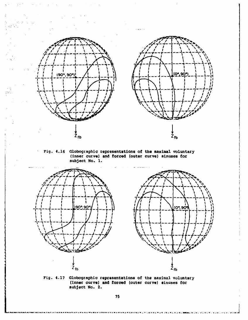
(90l - I I L--)--

.... cI o.- 1. ,

T•I ,'-' ' - ' - - -•• ;- ill t4• - - ,\ -- -• -• - -,zi ; :\ I • • ,,

' a o€*l I, ' • I \[OjO*

I A/\ '-* -- -'- ------------

I ' • : - - " - N-- . . ..

Zfb Zfb

Fig. 4.16 Globographic representations of the maximal voluntary(inner curve) and forced (outer curve) sinuses forsubject No. 1.

/" / _/ ' 7 \,

-" / ' , l, , .,,' , /• .. .I- - • ._ _

/ l : i ;/I\• ,i , ,I; 9. _ I(900,90o)/ I L............. - (O,9-' ' - ---i- -' --, , i /i ,, -- , - - -- "---, ,- -,' ., ,,

kk 21 /- ig ' ' '/7 :, -, -, -----.- /--,•---J , 3 .....j------ ----- 4

I I

Z fb Z fb

Fig. 4.1"7 Globographic representati ons of the maximal vol.untary

subject No. 2.

75

4 ~MW f~. a 4 * *~ V. t- £2 - J.~ W~J

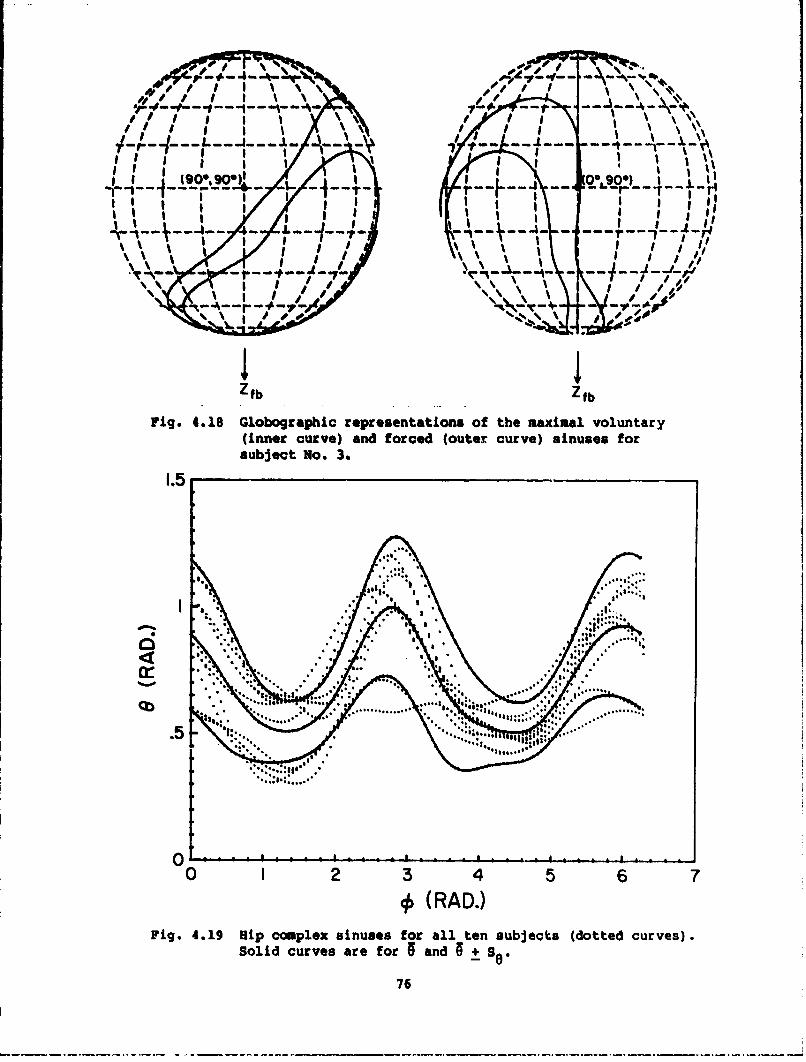
I I P

~I I I I

4 44

Z lb Zf

Fig. 4.18 Globographic representations of the maximal voluntary(inner curve) and forced (outer curve) sinuses forsubject No. 3.

'.3"

.. .. . ...

...........

*(RAD.)Fig. 4.19 Hip complex sinuses for all ten subjects (dotted curves).

Solid curves are for 9 and 9 + see

76

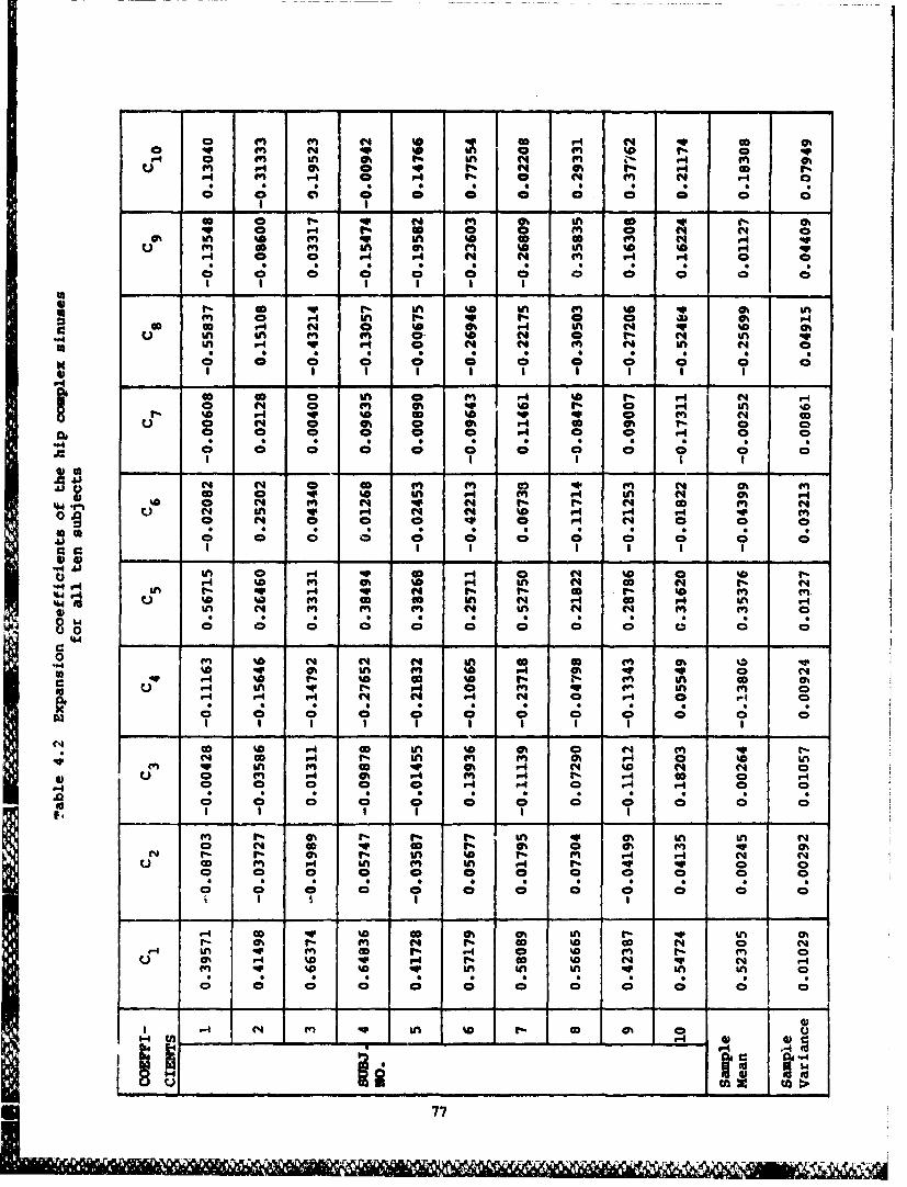
-n - - - - - -a% -

m 1% No S M V% P. OD r oH %

00 qv 04 eP n 0N InI co io f% co 0 0 r" N N% P. Hn (q 44 in % a co m M N 4

0 0 0m CD 0 0 0 0

o a a~C C',C C C

oo Go P. N 0 %D n N qr %D-w4C %n P. m 0q C % 0 M ý C4 %N N

cc Qn L sn r. 0 %0 1-FM N H-

* 0 0 C" 0 0 1 %0 r 0 5q M- %D r4 V % 0 0 %D V 0 C" 0

M~ ~~~~ CD n P.P 00

N 0to 0% HD SnM m N Mo M0 eq f" eq qv N V. P.4 N cc n

in H r4 Hr N Na N n

%S w 0 0 0 go Sl N 1- w04

inC C Ci A i e! C Ci C C 19

0 0 a S 0 M H to 40 H 0 H

0. en % N N k% to P 0 H" mSnoIin mo %D P4 0% toV

I I N i I 1%0 0 0 0%I P. 0k C; 0 C H C 0

.9o %0 r4 co Ln %D m N 0n

r in q cc 0 m 4 C0 %0 01 C4 a

NC N; C ; N0

D4 c t- In in qv S 0% 0Hn

o N4 CD qv CO r 0 H N% C r a%.I4 t-C C h r- %C %a t- en C C 04

OI m "4 in C In m f% 1 I

o- Ho qv %a HI 0% Np %o r- t P.fl. a%0 % C D c N P. N&M.I -0 Mo (a r% r 0 Mn N- H 0 I

0 80 0 0 )

-4 C4 M% Sn kn Wo H- a, 0 C0. M n U . H C P nP

H 1N HN-4K 0 5 5 0 S Su

C C a a a C C 0 0 C 77

\ . ..% .. . . ,1

71

! I I i ~ ~(90 4,90 .) / . !, ) .\ l , , '

S,~ , I ' ~ / l II/ q\I

4 - -- - J

~r

NI,-

I .I ---I- - -/ + ->-lI ji- -- - • - -+ . . . . .. -..

, I \g / ' / , I '••[ ' l I l

1 1

Zfb Zfb

rig. 4.20 G].obogra~phic repr'eserntations of 0 and S + S *

1.5

•O+Sq

F 'ig . 4 1.20 .Glnbographic r oepre I Eeenttuo B and ±S 0.+1lcb

4)(RAD.)

Fig. 4.21 and 0 + S 0 for two different runs.

78

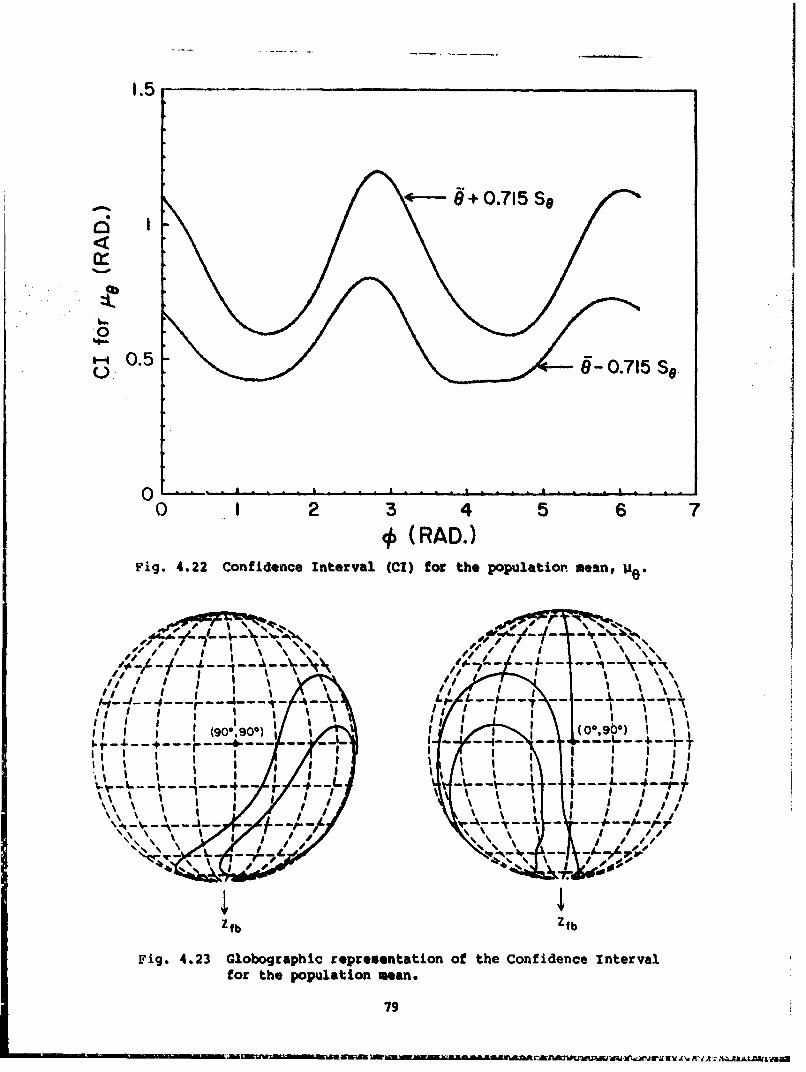
1.5

..-. '08+ 0.715 S&

-0.58-0.715S9

0 ! 2 3 4 5 ý6 7S (RAD.)

Fig. 4.22 confidence interval (CI) for the population mean, )y"

6' O

ItI0*0

'-S_

-(__ g..o • -- '• go 90) ,,

(00

.- --, - ---

0._.__4_ r__• _ 2 3.4.. 6.

Fig. 4.22 lbgahcrprsnaino h Confidence Interval RA.fCor foe poplaeo mean.ir~fl

, ,, ii ,;,, -•~~~--i-. ..-- •-r

/ I I Is

eo th ipOL]a.o Iean

79

I,~~K AN g-L (90190) XI (09

0 4 in C 0P-4 C4 P4A a 0 fn.4 r4 e-4 e4 P 4 '. 4'4

to N a N'0 4 fn N 4 0 N -4 4n

'0 0 ~~~ 0% 4-4 N 0 Sn 'N

P4 (.4 0 n 0 0 (-4 0DC*~~~4 Co n ' n M .4 0 044 N q

U 40 on*I 9014 co m0 0 0 S 0!%.-

4 Ln

at f-4 C) C4 co* % N 0o fr 0%n .4 N

%4 Sn cl N " 4 qN N4 NO4a

CDr- 4

4441 C" w- in 0% 0 % 4% 0 -

at --4 v-4 44 Ow ccOn G-~~C - - - - -

0% ~ ~ f LA '0C40 0N Sn*l

co ND N0 tN t0

0 n S 0 % ,4I.,40% P4 0% en cc N C45 ~ 0

"Sn tN N4 m0 0ý C4 .- NSn~~C .4 uI IrN 4 C44 .-I4

(.4

CI 0 n '0 n '0 0 N 0%

M tM co "V '0% cc %De0u- 0

Nw .-o Ch 0p '4 C4 .-4

II OT C

80 - -4

Ul ~ M ~ T & MFAhX z ~ A v ~

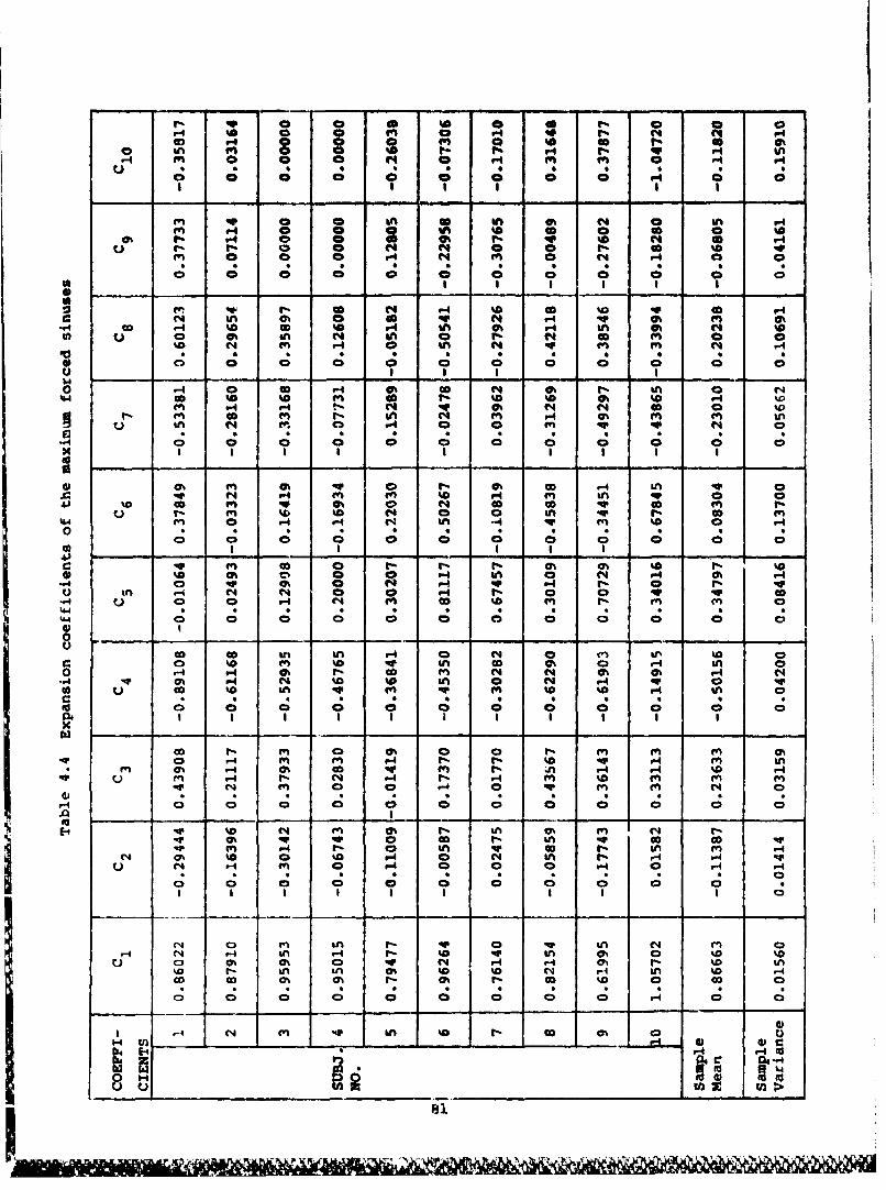
f" c ES~o F4 v t 0-

NP4

0 0 Im C; C; 9 0 0

mo * 0 a in % to0 0 p4 0 %a

r. fl o V 0 VI 0 N 0 f% %D q

a1~- 0 a aI 0 CD 0 0

C4 in 0 0 0 1.4 aNou 0 at in N 4 0 o M 0

kv 0 0 p N P1 m c" C4 04

0 ~ -10 0 to 0- at 0o C4 0 04

*0 -D --0 r D D

A m t-4 A qv10t4 ( 40 0 pM to m% %A 0 4 m 0-4 (q Pl in

in e4 M. i -4 0 VI Nw 49 eq C*0 0 0 0 0 0 0 0

o 0 a Q

o* '-4 0% 0- 0% 0 qVI 0t4 0 n UP %D Co 0 LC qC 0% % co C"

P1 4 en 0 4 N- LM - N a P4 I00 P I N P 4 0 1P

o0 %D N o 0 0- 0 0A a1 4 4' C% P040 9r 0 0 0i r4 90 04 0 9ý v

-4i 0 4 N 0 0 -0 0 0 0 0r r 0o0 "4 4 aO %a m rI a fn 2

44

o 0% P1 In 4 Co N% 0 V)I VIA w: %P en %0 v1 %n coI ( CD r4 in 00B 0- V4 0% r- to N N N 0% M PI N

.. v1 Ch N4 N D % 0 NI V4' 0 Cto. P1 0D p4 u-I f" VI %a4 4' M9 C

00 0- 0 Q 0% 0 CD I- fn (n m

m ai P4 C% 0o qv M- VI 0n N- u %0 r-4M r4 N - N P4 r* r-4 m %D t" m

-' Ui 00 0! uI N P1 01 fi 491 0'90 10 CD 0 0l o 0 0 0D C 0 0

0m__- e - -- - - I- -n f r-

Q -4

C~ 0 0 0 0 09 9 99

0 0 0 0ý 0 0 0 0m 02 0 0 0

0 ) M% P1 0 - RV 0 I' in C4 m 0%U4 04 P1 &n p.4 r- IC 4' tm0%D%

C3 M- a% Nk qvI C4 r-I P Im fl- %D%D Nl P1 0 0% to 0D N P %a Nr0C) C? 9 ~ 0: 9ý 9ý 9 99

u- 0 0 0 0 0 0o 0 0_ _ _ Ir_

0U--------------------------------------- _ _

u- to N n 0% 4 V vE' 0% 4'> 0 0 4% V 4 i04' P1 r4 4 0 V 4' 0 4% V8P1

q

(-2.5, 2.5), - (;, , <',')

(-2.5, -2.5) (2,5,-?. )

Fig. 4.24 Sample means of the passive resistive property,mlauni voiuntary sinus (inner dashed), andmaximum forced sinus (outer dashed).

P

(-, -25 2.!))) i

I J/ I I - ,- /"

Fig 4.2 Sapl means oftepsiersitv rpry

Ile/

--- - -i. . -- -/-i-- L .4--!I" 'T I - - -I .. .1 - - ' "-/ - . . .i

I- - -. I-- I .*. .. L. . .. ,,

I 1

Zfb Zfb

Pig. 4.25 Globographic representations of the sample '.eans of

'-he maximum voluntary and forced sinuses.

82

5, SIOINAM ICAL PROPRRTIES OF THE HlUM HRUERO-ELSOW COMPLEX

5.1 Introduction

Wao types of data are considered in this chapters (1) the maximum

voluntary humero-elbow complex &inus, or, the angular range of the

extreme allowable motion of the lower arm with respect to the upper arm

whose axial rotation is permitted, dnd (2) the passive resistive

properties beyond the full elbow extension with the lower arm in

pronation.

The elbow complex is composed of three articulations: the

humeroradial, the humeroulnar, and the superior radioulnar; it has been

modeled as a trochoginglymus Joint possessing two rotational degrees of

freedom (flexion-extension and pronation-supination) by most

investigators (Dempster, 1955; Steindler, 19731 Youm et al., 1979). By

utilizing the inserted Kirschner wires for defining coordinate axes and

biplanar radiographs, Chao and. Morrey (19791 were able to accurately

isolate the three-dimensional rotation of cadaver forearms under passive

elbow motion; the translatory components of the joint motion were ignored

by assuming that the tight ligamentous constraints would limit such

motion to small magnitudes. The additional component of rotation is

referred to as the carrying angle (or abduction-adduction). Chao et al.

(1980) also developed a device similar to the electrogoniometer for

determining the three-dimensional angular motion occurring at livingnormal subject's elbow joint while performing different daily functions.The carrying angle normally disappears when the lower arm is pronated

with the elbow in full extension. Due to the articular check (between

the olecranon process and fossa) and the ligamentous constraints,

excessive elbow extension beyond the maximum voluntary range may cause

serious injuries.

5.2 Determination of the Hlumero-Elbow Complex Sinus

Both kinematic and force application tests for the elbow joint are

shown in Fig. 5.1. This figure also shows the upper arm restraint

fixture. The fixed longitudinal axis of the upper arm with respect to

the torso Is chosen to coincide with the z-axis of the statistical mean

joint axis system established frr the shoulder complex in Section 3.2.

83

,I%

_ _ 1.6

i%'

Fig. 5.1 Kinematic and force application tests for theelbow complex.

In the author 's opinion, by positioning the upper arm in this

orientation, the shoulder complex is in a state of maximum laxity. As

shown in Fig. 5.2, the mean joint axis system is uniquely obtained by.4 first rotating the torso axis system by the mean angle ) (= 590) about

the zts-axis and then rotating the intermediate (primed) axis system by

the mean angle e (= 790) about the v'-axis. In this study, this meanm

joint axis system is also naturally selected as the fixed reference frame

(fixed-body axis system) for performing the kinematic analyses of the

forearm; the origin of this fixed-body axis system is conveniently chosen

S. to be the center of the humeial head.

84

~~M;SIMN

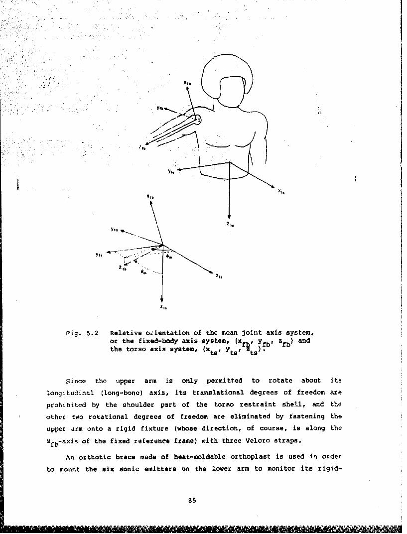
X~I

zt,

,t -,i-n

Z xts

ZIS,

rig. 5.2 Relative orientation of the mean joint axis system,or the fixed-body axis system, (xfb f'zb and

!i.'~fb .Y b ,'..." .', ,,

the torso axis system, (x, t' ,. . z,

since the Lipper arm is only permitted to rotate about its

longitudinal (long-bon~e) axis., its translational degrees of freedom are

prohibited by the shoulder part of the torso restraint shell, an~d the

other two rotational degrees of freedom are eliminated by fastening the

upper airm onto a rigid fixture (whose direction, of course, is along the

z fb- axi of the fixed reference frame) with three Velcro straps.

An orthotic brace made of heat-moldable orthoplast is used in order

to mount the six sonic emitters on the lower arm to monitor its rigid-

85

boiy kinematicsi. iw ecosrp r sd to,ý hold the br~ace oil the

lower arm* .In addition, by letting the hand hold a pole which extends

from the brace, the wrist aomplex is fixed so that the forearm muscles

are held in a stable configuration.. This orthotic device. thus eliminates.

tht relative shifting motion between the forearm and the brace. The

forearm cuff with six eMitters-affixed to it is then rigidly attached to

the brace by two screwsý 'The forearm cuff ie made of a rA,6id,

cylindrical, rlastic shell which extends about three-quarters of the way

around the lower arm. It is believed that this orthotic configuration

comes as close as possible to rigid body conditions, and, provides for

accurate measurement of forearm kinematics,

The procedure for quantitative determination of the humero-elbow

complex sinus consists of the following steps% (1) immobilizing the torso

and upper arm, and defining the fixed body axis system as described

before (also refer to Fig. 5.2), (2) having the subject move his forearm

along the maximum voluntary range of motion and continuously monitoring,

with respect to the fixed-body axis system, the 3-D coordinates of a

distal point on the moving body segment; this point (to be referred to as

the wrist joint reference point) is selected as being on the longitudinal

axis of the forearm at the level of the styloid process, (3) fitting the

wrist joint reference point coordinates to a sphere using the le3st-

squares method, thus establishing a center for the best-fitted sphere and

an idealized link length (radius of the sphere), (4) fitting a plane to

the same wrist joint reference point coordinates using, the least-squares

method; the normal to this plane (specified by the sphe:ical coordinates

1•n ) as shown in Fig. 5.3) establishes the pole (x -axis) of a localn n it

joint axis system (for the humero-elbow 'complex) with raspect to which

the humero-elbow complex sinus, designated by the spherical coordinates

($, 8) of the vector connecting the center of the best-fitted sphere with

the wrist joint reference point, can be expressed as a single-valued

functional relationship, i.e., 8 %(OW.

Since only the wrist joint reference point is monitored, the same

initialization procedure as that used for the hip comlex is employed.

Before the humero-elbov complex sinus test, the subject was

instructed to move his forearm along its maximum voluntary range of

motion in a counter-clockwise direction as viewed from the sensor

86

Xit

yj,

Yfb6

Z~Zfh

Fig. 5.3 Reld~~ltieoinaino th fie-oy(b fb

Figmh~. 5.3Relative orietaton of the foiear d-bout (x5 it longtudnlai

was l1-ft~ up to the ditscretion of the subject in obtaining the maximum

sinus~. Several swe.eps o~f this type were practiced before data were

co~llected so that the subject could experiment with obtaining the largest

possible range of motion. In order to help maintain a constant

07

rate of motion during data collection, a large clock with an easily

visible second hand was placed in front of the subject. The subject was

instructed to imagine his forearm as the second hand, and to synchroniz'

his circumscription with the clock's 60 second sweep. The firing rate of

the sonic emitters was set at seven data records per second (as used for

the shoulder and hip complexes) so that a total of 420 wrist joint

reference points was collected for each complete humero-elbow complex

sinus.

Table 5.1 lists the centers and radii of the best-fitted spheres and

(On 1 8) values of the best-fitted planes for all ten subjects. With

respect to each individual local joint axis system designated by

(On I )e n Figs. 5.4-5.6 show both the raw data and least-squares fitted

values of the single-valued functional relationship, i.e., 0 = 9(f) of

the humero-elbow complex sinus for three subjects. In these figures,

only 72 raw data points (approximately equally spaced, were plotted and

used for curve-fitting of the functional expansion, Eq. (3.2.1).

Figs. 5.7-5.9 display the globographic representations of these three

functional expansion sinuses with respect to the fixed-body axis system.

5.3 Determination of the Passive Reaistive Properties

Beyond the Full Elbow Extension

Since the force applicator is constrained to motion in a levelhorizontal plane by a track-mounted trolley system located overhead, it

is necessary to tilt the torso, while sitting, 110 (= 900 - em) about

x -axis so that the upper arm is also parallel to the ground. Thetisubject was first instructed to pronate his forearm to face the ground

and to fully extend it. The force applicator was then positioned

vertically at the same level as the subject's forearm, and the transducer

front was positioned near the wrist joint. The subject's forearm was

next forced beyond its full extension in a quasi-static manner until the

subject started experiencing discomfort. During the entire course of the

test, the subject was instructed to let his forearm hang limply and not

to actively (muscularly) resist the motion of the test.

The data collected according to the foregoing procedure were

analyzed as follows. First, the force (P) and moment (A) vectors

obtained from the force applicator transducer were used to calculate a

88

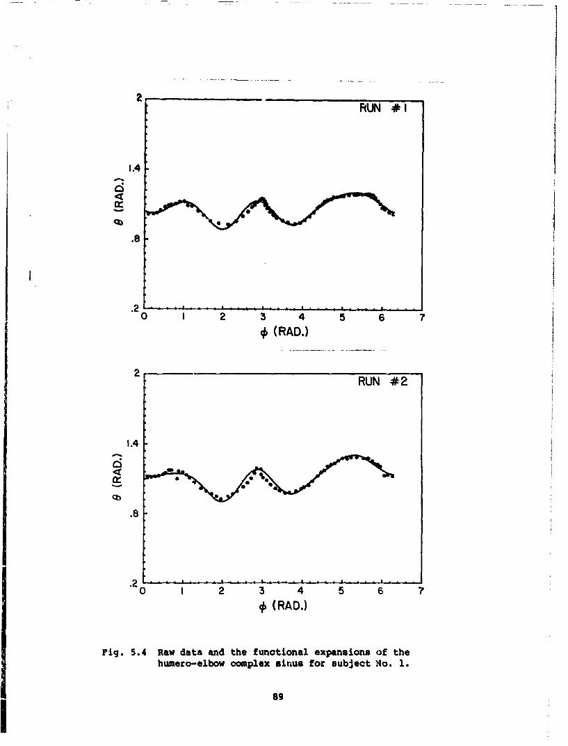
2 RUN *I

1.4

.8

0 I 2 3 4 5 6 7* (RAD.)

RUN #2

1.4

i q• .8

• 2 o .... .........;,, . . . . . . . . .5• ".. .•0 1 2 3 4 5 6 7

* (RAD.)

Fig. 5.4 Raw data and the functional expansions of thehumero-elbow complex sinus for subject No. 1.

89

2 - -RUN * I

IA42.8

.2 -- - - - -. . . . .• 0 1. . . . 2 ' ; 3' ' - ; • • ' '": 4 5 6 . .. 7

S(RAD.)

2 RUN #2

I

0 I 2 3 4 5 6 7

(RAD.)

Fig. 5.5 Raw data and the functional expansions of thehuwero-elbov complex sinus for subject No. 2.

90

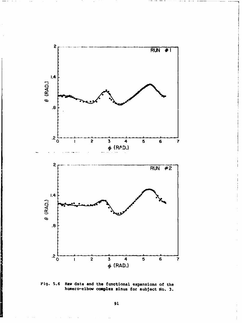
RUN I1

1.4

.8

0 I 2 3 4 5 6 7* (RA.D.)

RUN #2

1.4

.8

0 I 2 3 4 5 6 70 (RAD.)

Fig. 5.6 Raw data and the functional expansions of thehumero-elbow complex sinus for subject No. 3.

91

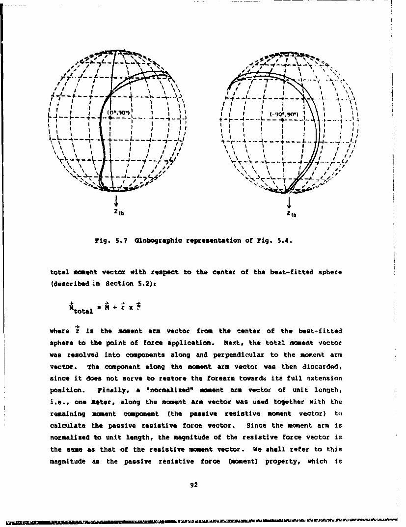
"I, , ;r' \", ,

.e4--•~4- L.2"r),,••, ' ,'II I I I \l I e ! I ! ' • I -

I ! I I I ! I I ,I II I I I IIi_ . , , ,, ,,

I+

\\r r -

,.:.6- - - ' .-- , • .

- I •. 1 . •-

Z fb tfb

Fig. 5.7 Globographic representation of Fig. 5.4.

total moent vector with respect to th. center of the best-fitted sphere

41J

(decrbe den Setin5.)

where r is the moment arm vector from the c enter of the best-fitted

sphere to the point of force application. Next, the totel moment vector

was resolved into components along and perpendicular to the moment arm

vector. The component along the moment arm vector was then discarded,

since it does not serve to restore the forearm towards its full extension

position. Finally, a "normalized" moment arm vector of unit length,

i.e., one meter, along the moment arm vector was used together with the

remaining moment component (the passive resistive moment vector) to

calculate the passive resistive force vector. Since the moment arm is

normalized to unit length, the magnitude of the resistive force vector is

the same as that of the resistive moment vector. We shall refer to this

magnitude as the passive resistive force (moment) property, which is

92

(0 . o . . . ... "

1 L- '- --i 4--- AV_•, __-" -- -"'--•- - •--"

I ! \

, .6,0

expressed as aI func o, a ' • a i f telbow extension In cg ts ,le, (-90,90 . ,i_ ,on..i

center .... M--e ....st-fte -- p-h-., e and t -h -disalwrstjontreernc

Figs'. 5.0-.1 sho tw run of', both th rawdat,,.,hcuve

I., \ \, I l s s s,", I 1 •

"".'.-, , I /,_/

Zfb Zfb

Fig. 5.8 Globographic representation of Fig. 5.5.

expressed af a function of th, or the angular displacement frop the full

elbow extension. In calculating this angle the line connecting thecenter of the best-flitted sphere and the distal wrist joint reference

point is used as the longitudinal axis of the forearm.

Figs. 5.10-5.12 show two runs of both the raw data and the curve-

fitted function values of the passive resistive force (moment) properties

for three subjects. The expansion function used is of the following

polynomial form:

f(Mx) - C 1 t C2 a + C3 a 2 + C o43 (5.3..)

5.4 Statistical Data Base for the Biomechanical Properties of

the Human Uumwero-Elbow Complex

Since the functional expansion used for the humero-elbow complex

sinus is the same as that used for the shoulder complex sinus, the

statistical procedure is the same as discussed in Section 3.6. Table 5.2

93

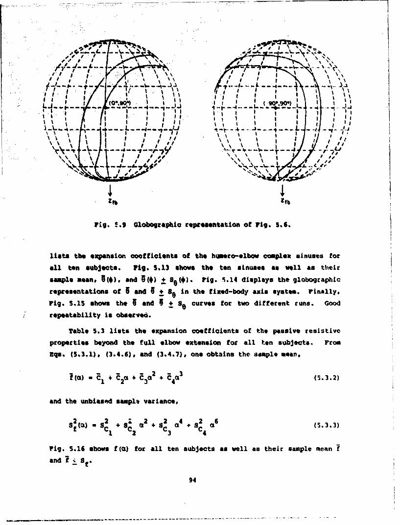
• W.W " \ W%,

i I I I I,•i ' X , '

A S.. .l , -1 ! , !' i • , ! ! i I i\ , 4• . I I • ! .. .I I t I.I 1 i _ . r l ! i I I I ,

ii iI t I " Ii- ! . IIII ! ! I i !

t ! I I i I I I g I , I

\ \ * -!

' ,'' ,' \ ', ! I ' ',X', It I1 / ,,, , ,-,

IF OF

PLg. S.9 Globographic representation of rig. 5.6.

lists the expansion oeofficients of the himero-elbow complex sinuses for

all ten subjects. Fig. 5.31 shown the ten sinuses a4 well as their

sample mean. §(t), and so() ± ) Fig. 5.14 displays the globographic

representations of I and + 8 in the fixed-body axis system. Finally.

rig. 5.15 shows the 6 and • ± S. curves for two different runs. Good

repeatability is observev.

Table 5.3 lists the expansion coefficients of the passive resistive

properties beyond the full elbow extension for all ten subjects. From

Rqs. (5.3.1), (3.4.6), and (3.4.7), one obtains the sample mean,

() - aC1 + C2ai + Ca2 + C 4 a3 (5.3.2)

and the unbiased samplu variance,

S 2 ) a S 2 + 2 ;a 2 + 12 a 4 +2 a6 (5.3.3)3f ~C I ~C 2 C 3 C 4

rig. 5.16 shows f (a) for all ten subjects an well as their sample mean

and Sf.

94

30 soS RUt #1 RIN *2

t.o t.oz

10 I0

0 0t 15 20 25 0 5 10 1S 2 25a (DEG) a (DEG.)

Fig. i,.10 Raw data and functional expansions of the passiveresistive property for subject No. 1.

30 r- 30,RUN #1 RUN #2

20 .20

z zz z

10 10

5 to 15 20 25 0 5 1I 20 25

a (DEG.) a (DEG.)

Fig. 5.11 Raw data and functional expansions of thepassive resistive property for subject No. 2.

95

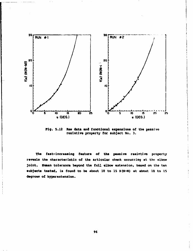
30 30UN # eRUN #2 2

_20 20

10 10,"025 00 5 10 IS 20 25

2 (DEG.) * (DEG.)

rig. 5.12 Paw data and functional expansions of the passiveresistive property for subject No. 3.

The fast-increasing feature of the passive resietive property

reveals the characteristic of the articular check occurring at the elbow

joint. Human tolerance beyond the full elbow extension, based on the ten

subjects tested, is found to be about 10 to 15 N(N-N) at about 10 to 15

degrees of hyperoextension.

96

1.4† † I .. ...........

C..

Fig.8 5.3Hmr .lo cmlxsnssfr l e ujcs

Solid curves are for Band + See8

.1 td L.

(0-10-) -go.900ii 4 JJL 4

I f '

II -~-4=-------~---L - - J

0.~~ I"~&nnW P(/17/ f W0 n - VIfn,.m~UM- wM:A"X40L -n J~ "/I ,'-IU 7'fn&RR LA~ & - tf~ nfnAIAAf~

1 .4 O+..8-,

.2 '0 I 2 3 4 5 6 7

S(RAD.)

Fig. 5.15 e and B + S9 for two runs.

98

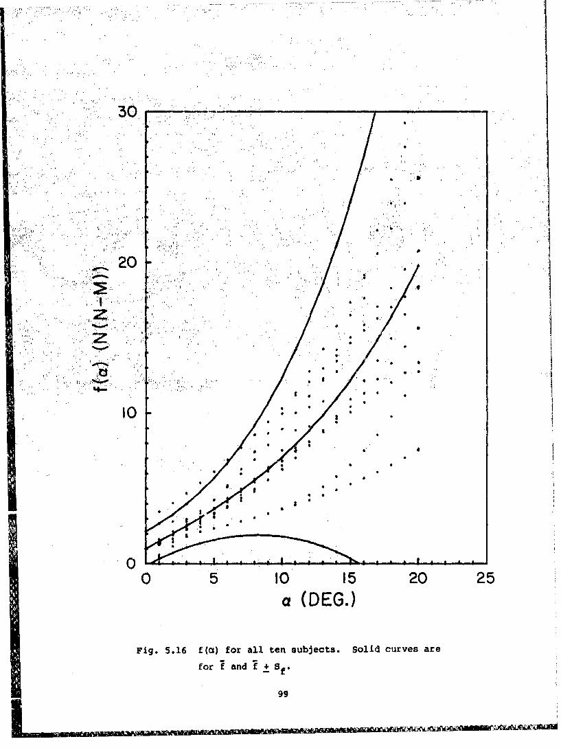
30

.-. 20

10I.

999

Table 5.1 Centers and radii of the best-fitted spheres~and 0~ for all ten subjects.ý

n

SUJCT 'CENTER (ct) RDU

No. xf f f (cmt) (deg.) '(deg.)

1 -0.06 0.19 28.76 29.58 -57.25747

2' 0.43 0.12 25.90 29.62 -40. 57 71.42

3 0.69 0.96 27.11 29.72 -57.51 70.92

4 1.62 -0.20 28.14 31.12 -43.44 70.21

5 -1.22 -0.30 22.09 28.38 -67.33 58.75

6 -0.72, -1.51, 25.00 29.93 -55.06 66.69

7 -0.77 0.88 26.79 30.96 -42.73 7r.45

a -0.43 0.66 27.73 30.24. -53.74 68.01

9 -1.27 1.01 26.90 29.39 -37.92 71.99

10 -1.10 0.21 26.51 28.69 -55.70 59.94

Sample

Mean -0.42 0.20 126.49 29.76 --51.14 68.98

SampleSt. Dev. 0.89 0.76 1188 0.87 9.460.7

100

0 C4 rn 0o % H r-4 0a N 0 Nýoý WD r- Ný 0% C 0 H r- r- %D In Nl

r,4 0 ch (~4 km 0% in 00 9- mC. 0 H t-40 H P4 to 9. In

on CD H- Ho ONN H ~ 40

o4 0ý 04 H Q 0 0 0 0

-4 %0 4 0o N 0 LA a t-

oE CID0 cl 04 (4 en Co N In %D

a% C3 C) v% C)' '40 Q C)

U0% Htr -0 % No %n C) to W4 HcH0 ~ ~ m O %0 o %D H H %0 %D 04 0 %D

o4 0ý. 1 1 0% 0 r4 V %0 0 0 0 0D 1 0

4) M0 N 0H H N (n 0CN

c; l CO ' t) 40 C) c; H I

.C o 4 0 l CO Hn Hn 0n H0 H HH

M o" CA 0 0 N 0% 0% 0 0r 0l 0% 0

0O N U, I 0 4 C3 0

41) j C) H> ClN C) CO:1H Cl )C

0o %0 40 4 -W r4 m i I- %a%

0- 0 00 0W AM 0- 0 N 0o 0 0t0

X.4 44 CD Ql IAo C0' VH 00 N 3 COý Ql N0

0 ) c0 m. 00 40 0 -1 In %D . 0% 0 eC Oin U) mn OD fn 0D %D M Nt

OC 0 H- CLh (= c 0 Cl Hn Hn m %00 Ctoj 01 0> 4 0 0 ) 0 m C 0 04 0 0

0D .H N 0% 4 0 ( % ,tO3 (A 0I m 0n H 0 0 0 HD 0o 0

1ýI Il I i *l r tC

6wp 0 C~p C3 0D ý 0 '0 0 0n 0

-W in H n 0 co 0n H0 Do %ON CY% CIS H C0 0~ 05 0 r Go

a) Hr in 0- C" IA co Go -04 Cc4 : (n 0C -4 a. 4 m

C' C73 0 C2 0 t0 0 0 0;

CD4 Io CI I4 VI ko L 1Uim

k* '.0 () 1 "% Cl 0l Cl C> D mI-Ae(;4 %D 0 00 C'. C4 0% q 0 mn 0or 1

IA U) l C" CT 0 H- CO mO co NHH C:) N DD eq -4 D Cl

r- 4 c; r! * IK - *--- _ I.. __7

-r4 M -t-(") %D 0- co n 40 04wD E-l r4 m N44 CO t- -4I C

o CO l L 0 z mO H>I I S I 01

am= III I _

Table 5.3 Expansion coefficients of the pussiveresistive properties beyond the full elbow

extension for all ten subjects.

005FF- C 1 C 2C 3CI-M

1 -0.29505 0.97641 -0.04239 0.00167

2 2.62520 0.12251 -0.01258 0.00397

3 1.21570 0.41974 0.04335 -0.00077

4 0.99568 0.36091 0.06439 -0.00104

SUB3. 5 0.97960 0.40776 -0.03570 0.00224NO.

6 2.99000 0.47401 0.03703 -0.00111

7 -0.38531 0.81571 -0.01229 0.00029

8 1.00290 0.48261 -0.00950 0.00143

9 -0.28201 0.81601 -0.04942 0.00465

10 1.25800 0.22501 -0.00158 0.00031

SampleMean 1.01047 0.51007 -0.00187 0.00116

SampleVariance 1.32818 0.07543 0.00148 0.00000

102

6. JCONCLIVDING REM&RK

In biomechanics research, many random variables associated with the

human body are either normally distributed or have approximately normal

distributions. Therefore, a sample of size ten utilized in this research

is expected to provide reasonably good statistical estimations from the

analyses presented herein. All the results were presented in a compact

format and can thus be easily incorporated into the joint complex regions

of the currently existing multisegmented models of the total human body.

From a safety design point of view, the maximal forced sinus data

presented in this work can be considered as a prelude towards

establishment of a criterion for the impending injury on the joint

complexes studied. Any support/restraint or protective device should

have the capability of restricting the range of motion of the moving body

segment below the maximal forced sinus under most types of external

loading conditions.

In conclusion, it is important to point out that biological

materials, especially soft tissues, display nonlinear viscoelastic

behavior. If we assume that the passive resistive response of the soft

tissues in the joint complexes can be modeled similar to the Kelvin

viscoelastic material, i.e., elastic and viscous forces are additive,

results presented in this work can lead one to the determination of the

elastic component of the passive resistive force (moment) on a particular

soft tis:-ue. Thus, the next important research endeavor should be the

determination of the velocity-dependent viscous component of the passive

resistive force (moment) properties.

103

A~PPSMX At SUL2CTD AWU 0TIRZC MMAURUUNYS CW T3M SUBJKC!I'S

seeqb $69tgs via11 63 Is 3 734 set 114 714 f.9a3

statute 1.2 16 1.2 S) 13 12 6 160 0lt 1117.11

Ibsm.dr t~ufeses 365 2 13. 1 IN2.6 114.3 Lit.% O. 106. 1I 104.t

ftlot eireamftre~m 93 It 6 73.7 94 71 He 63.8 111 71.

ia lmeree16.6 16.4 16.9 17.6 1. 17.0 17. 6 17.6e I?.K 17.Lear arm ciomfo.Iresou 31.2 29.9 31.3 26.7 29.6 27.9 25.5 27.9 .141. 1 2a.t.-

ftoo" altumigmeW16 311.4 34.3 34.1 26.7 34.9 30.5 IQ.% 27a U.1 1 i.. 4j

'ftii. qpeg altSommfttUI .1 soSO 61.3 W-5 3. 64 S3.3 so S6.6 sa II)a

f1isih. lower circuiftueome 41.1 42 44 36.1 43.2 43.2 41 36.1 It 31.4

Colt ClrOUmfaegw39. 3? 39.5 34.9 46.6 40.6 42 11.4

Ankle aleirafotenoe 33.4 26.3 26.1 26.7 25.4 26.7 27 211.4 211 211.4

ltoner. -Wist length WS. 23 20.9 25.4 24.1 24 25. 4 27. 9 2%.4 22.9

Shoulder -elbow lsength I6 46 35.3 33 27.9 34 37 Is6. 1 MIS P

Shoulder m hight. sitting so 63 59.11 Of 62 60 70 Nt . . i

Shoulder breadth SO so 5 44 46 45 44 42 4h. 4

Chant bzeedth 32 34.5 31 31 33 32 34 JI 14 11

Chest depth 26 27 26 24 as 14 26 at 21 t

"Meit deptha2 24.% 25 20 24 is 24 21 11 IR

Buttock - kaselength 6 55 6 6 5 0 N S ~~Buttock - p"pliteal length 49 54 so 55 so so %a i0 %6 S7

Knee beight, sitting 54 67 55.7 57 53 S6 55 so .'

El1bow-telobget 47 46 50.5 44 51 45 4S 43 44 I19

NlIP breadth, sitting 39 37 36 37 39 35 41 is ai Ht--

KnaeII-to..knae breadth, sitting 25 22.5 23 20 23 Is A) a) al L9

1.04

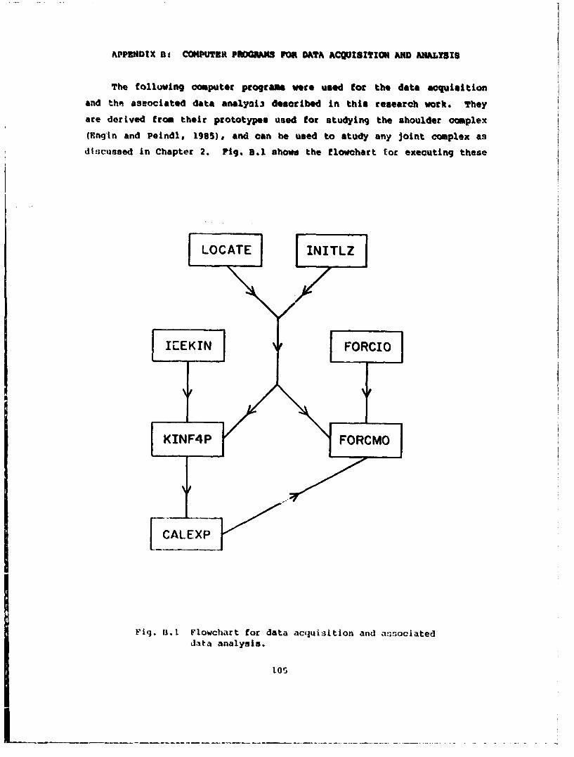
APPENDIX Bt CO0PUTSE PROGRAMS FOR DATA ACQUJISITIO AND ANALYSIS

The following computer program were used fot the data awcuisLtion

and tht associated data analyoi3 described in this research work. They

are derived from their prototypes used fot studying the shoulder complex

(Rngtin and Peindl, 1985), and can be used to study any joint complex as

dincussed in Chapter 2. Pig. B.1 shove the flowchart [or executing these

LOCATE INITLZ

KIEKIN) FORci''

KIN4 FFORCMO

FPig. B.1 Flowchart for data acquisition and associateddata analysis.

1O5

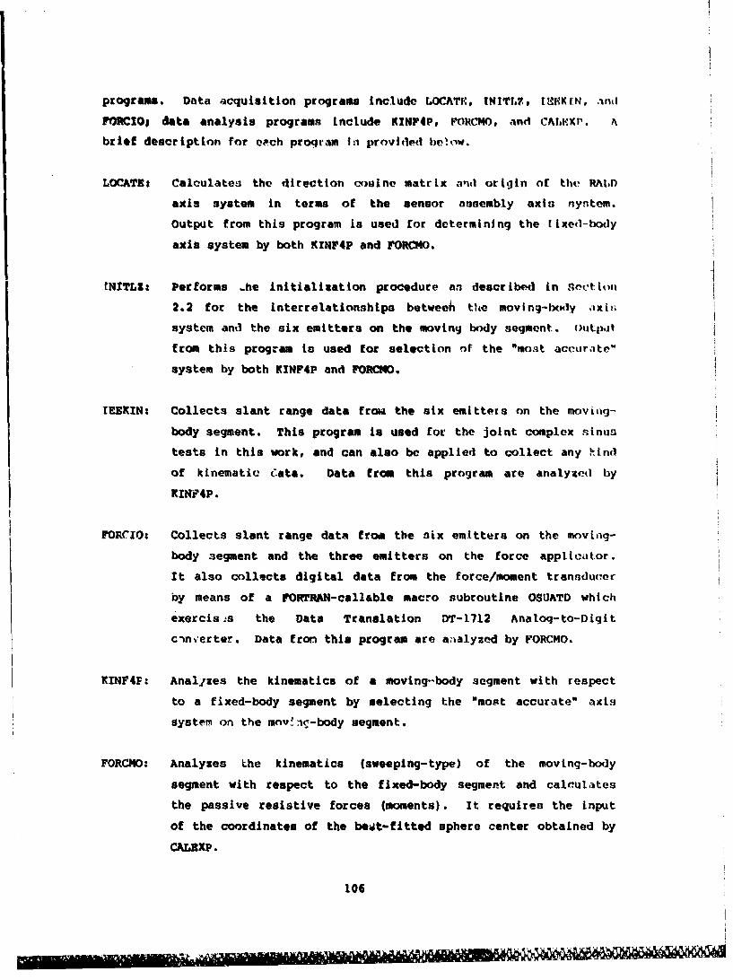
programs. Data acquisition programs include tOCATr., t~tTf.s, INHKMN, .knd

FOMCIOJ data analysis programs include KxNF4P, PORCHO, and C1I0,'X. A

brief description for epch program In provided belo.w.

LOCATEr Calculates the direction cou1ne matrix and origin or the RAIWf

axis system in terms of the sensor assembly axis nyntem.

Output from this program is used for determining the [ixed-body

axis system by both KINF4P and FORCeO.

INITLgt Performs .he Initialisation procedure an described in Sectioti

2.2 for the interrelationships betweeh the moving-boidy ,xin

system and the six emitters on the moving body segment. Outpat

from this program ti used for selection of the "most accura'te"

system by both KINF4P and POROMO.

TEEKINt Collects slant range data from the six emitters on the moving-

body segment. This program is used for the joint complex sinus

tests in this work, and can also be applied to collect any hind

of kinematic Cata. Data froam this program are analyzed by

KIN?4P.

FORC.IOa Collects slant range data from the six emitters on the moving-

body aegment and the three emitters on the force appliciltor.

It also collects digital data from the force/moment transducer

by means of a rORTRAR-callable macro subroutine OSUATD which

exercis -s the Data Translation DT-1712 Analoq-to-Digit

cin'0erter. Data from this program are aialyzed by FORCMO.

KINF4F: Analyzes the kinematics of a moving-body segment with respect

to a fixed-body segment by selecting the "most accurate" axis

System on the mnv _it-body segment.

FORCMO: Analyzes Lhe kinematics (sweeping-type) of the moving-body

segment with respect to the fixed-body segment and calculates

the passive resistive forces (moments). It requires the input

of the coordinates of the best-fitted sphere center obtained by

CALMXP.

106

I'lr'r'lA W _- ... . . . . . .

CALEXP: Calculates the center and radius of the best-fitted sphere to

the joint complex sinus by least-equares method. it also

calculates the best-fitted plane to the sinus and then

transforms the sinus data into functional relationship with

respect to the local joint axis system. Finally# the

functional expan,•ion of sq. (3,2.A) is used to obtain the

expansioin coefficients for the joint complex sinus.

I10

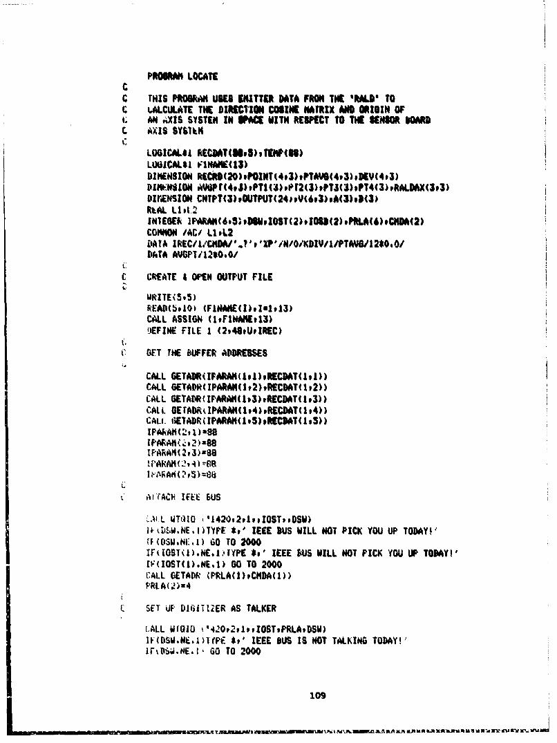
PROGRAM LOCATE

CTHIS PROGRAM MUSES MuTR. DATA FROM THE ORALDITt ALCULATE THE DIRECTION COSINE N~fRIX AND ORIGIN OF

t. AN .,XIS SYSTEM IN IPACE WITH REIPECT TO THE SENSOR WARDC AXIS sysiN"

L0GICAL*A RECOAT(Hi5),TERP(SS)LUUICAL*I FI1NANE(13)DIMIENSION RE[CRD(20),POINT(4,3).PTAVS(4,3),DE(4.3)PM.*081ON AYGPt14tS)9PTI(3S),i'2(3)#PTI(3)oPT4(3)PRALDAX(3#3)DIr1ENSION CNTPT(3),OUTPUT(24.,Y(6,3h*A(3).5(3)Rt.AL LIP.t.INTEGER IPARMe(6.53.DSWI0ST(2).IOSD(2),PRLA(6).CNDA(2)COMMNO 1ACi L1.L2DIATA IREC/I/CNDAD.?,'XP'/~N/0/KDIV/1/PTAVGI2*0.0/DATA A9GPT112*0*0/

C CREATE & OPEN OUTPUT FILE

WRIE D(5ol)(FNAE0*893

CALL ASSIGN (.v~lNAhE,13)44EFIHE FILE I (2948#UPIREC)

G3ET THE BUFFER ADDRESSES

CALL GETADlR(IFARAM(lt1)vRlEC9AT(1Iv))CALL GETAOR(IPA RAM (I.2)9RECbATll*2))CALL 6ETADR(IPFIARM4(I3)tRECIDAT(193))CALL OErADRtIPARAH(1v4)vftECfATl.4))CALL. (ETADR(IPARAN(1w5),RECDAT(1.5))

[PAFRAN(2v 1)288

1.PAJRAM(2w4) r(R

c AiACH IEEE EIUS

.A'll WT010I 0142092p1..IOSTopDSM)4tiUISW.NEJl)TYPF 1.' IEEE BUS WILL HOT PICK YOU UP TODAY!'

rF(su41:I)GO TO 2000IFUOGST~l)NEs.-t*YPE *s' IEEE 141S WILL HOT PICK YOU UP TODAYI#IF(I0ST(L)s*Eol) 00 TO 2000CALL GETADR (PRLA(1)PCIIDA(1))PRLAt.2)n4

c SET UP DMI1TIZER AS TALKER

(.ALL WI010 kl4.102v2IvvIOSTvPRLA9DSW)IH(DSWHI.E.11(PE *t' IEEE BUS IS NOT TALKING TODAY!'

1r~D~.NEt G TO 2000

1jl~tmm mts mlmm h~ufth~~tU m b~f~ru~dIXxUAi~.nd~~I 3 5i i 1. .9.U~\~iDLRM M R UMAMAM MAM ~M~10WVL M2

IfINGT(1),E-)TYPt W, ;ssi IWS 1 NOT TALIKIN6 TODAY'IP(@ST(l).NEol) 0O TO 2000

CC "AD IVIW SETS OF POINT VAI.0ESC

20 CALL VAITFRAl0)SO* CALL 010000.O~2.101.IOSDj~IPARANAKPJT),DW)

IM(OUNT.E*..) so TO 50W1 10 20

Si0 CALL WAITFRUO0)CALL WreI0(42000vlvS,,IlT,,s$W)CML CLRfF%10)

C CAtCULATE THE AVERAGE VALUK6 FOR THE FOUR POINTS

t53 60 100 KNTaI.5KDIOI .T-000 60 Il1.IseTEMP(Ma)RECOAT(HoMKT)

61) CONTINUEflECOSE (88400MHEP) (RECU(Kb).Keu120)IMAMS1) 60 TO 45TYPE W*SLAMT RANUE VALUES FOR FIRST NMIOAWRITEM5POG) (RECRD(WL-K) .K'20)

45 CALL COORDNRECR9#POINTvKNT)

IF(POINT(.JK,).NE*0,0)O0 TO 70WRITE(59560)KNT

TF(N*EQ*2) TYPE tv' TWO RECORDS CONTAIN ZERO VALUES.9 9'.101 FAILEDIF(N*EQ.2)60 TO 24M0so TO 100

;0 CONTINUEDO 90 .1.,4DtO 80 111.3F'TAVG(JI )aPTAV6(J.I)4POINT(JI)AVGPT(JI)aPTAVO(JtI)/KDIY

IF(DEY(Jol).LT.o.25) GO TO 90WRITEM(5540)

80 CONTINUIE"ZO CONTINUE100 CONTINUE

DtO 110 JJnI,3PT1 (JJ)aAVSPT~ .JJ)PT2(JJ)=AYgPT(2pJ~J)PT3(JJ)aAIJWTi3tJJ)Pi4(JJ)aAWOT(4pJJ)

110 CONTINUE

110

t-0 111 18113

00 1'12 V1*1)*2V96**4(.)*

..ALGULATE THE AXIS SYSTIN (RMLDAX) AND ORIGIN (CNTPT)DJO 120 1.1,3

At 1~uPT4(I)-PT2(I)9(1)=PT3(J)+1T2(I)

120 CONMTI"U'-ALL DftCIAT(ApbsRALDAX)

1101 130 Jjai#t.NrPT(J)*TI (J)-8,4914RADAX(IPJ)

130. CONTI"U10 140 Kmj,3

k-lITr"!(K43)mRALDAX( uK)3W1PU1 tKf6)aCHTUT(K)OUTFU[tTK+9 )-PT2(K)

cJrPUT(K+18)uRALDAX(3pK)ud!Fur(K+21 )=PT4(K)

ItALl. INFORMiATION IN DATA FILE

I*rE459600) (OUTPUT(I)v1m1.9)

~JPITE(5#800) (OUIPUT(I), 1=22v24)

WRITE (1'1REC) (OUTPUT(I).I91#24)

;'"i.L CLREFIO)l,.AAI('$,t'Ent~er the name to be siven to the data

',40 t'JqA~f('0v,'1NACCU&ATE COORDINATE--DEV* EXCEEDS .2SCI')'> -,Fmk4('OWsRECORD NUHI45f'pR 'vl5s' CONTAINED ZERO VALUES ANI)

ltt H., BEEN4 DELETED.')

390 F0TV*;'Ti49'POINT OgWftINATES'PtI52o'PLATFOAN AXES worot.

600 FOWAT(' ',TIO,3cr5,2),T5o,3cF9,4)~T92,3(FS.2))700 FORNAT40f' 'Tl03(FS.2)vtSO3(F9*4))600 FORMAW( ItT10,3(F32))820 F0WMTeO','T14. 'DIMENWNQAI CNECK'//V5''LSTH (1-2,1-3,l-4)a4,

11B3ch'tT409'LGTH (2-3p3-4t4-2)-7#67gg'v/)840 FORMAT' '.TIO. LGTH12atTlSF5,2,T45,'LOTM23s',T53,F5,?/I

It1O, 'LOTH13=' ,TIS.PS,2.T45.'L6TH34m' .tS3.P'52/ItlO. 'LGtH14u',T1S.F5.2,T45b 'L8TH42a',t533P5,2)

900 FORhAT(0'O'4(F3#0y4F'7.2t4X))2000 STOP

ENDC,C

SLMWTINE DRCMlAT(A.R.C)CC THIS SUBROUTINE CALCULATES THE DIRECTION MOINE MATRIXC FOR AN AXIS SYSTEM DAME ON rWO COPLANAR VECTORS (A and 3),C THE RESULTING MATRIXt* C, IS ORTHOGONAL AND UNITARY.c

DIMENSION A(3) .3(3) .C(3t3)AMAGuBGRT(A( 1)**2+AC2)**2+A(3)**2)BMAG-SQRT(S(1 )**2+3(2)**2+3(3)**2)C (2pl ) mA(1) /AMAGC (2p2)uA( 2) /AMAG

C(23,)aD(3)/AMAGC(3v2)u3(2)/8MlAGC(3p3)=B(3;/BMAGC(1,1)-(C(2,2)*C(3,3) )-(C(392)*C(2.3))CU ,2)a(C(3,1)*C(2.3))-(C(2.1)*C(3,3))

C(3,2)=(C(2,1 )*C(1,3))-(C(1e1)*C(2.3))C (3,3)a(C (11) *C (2.2))- (C (21) *C (1.2))DO 10 J21P3CMAGsSGRT(C(Jp1)**2+CCJt2)$*24C(JP3)**2)DO 5 7&w,3C(JtI)=C(JI)/CNAG

5 CONTINUE10 CONTINUE

RETURNEND

SUBROUTINE COORD(RCZD)ATuPOINTPKNT)cc THIS SUBROUTINE COM4PUTES THE XtYtZ COORDINATES FOR THE SPARKc OAPS IN THE BOARD REFERENCE SYSTEM DY PERFORMING CALCULATIONSC ON THE SLANT RANGE DATA FROM THE FOUR CORNER MICROPHONESC

DIMENSION RC2DAT(20) .POINT(4t3)

112

DATA Lli'167,75/t UL2/1116ip KIi/3.90t*LASE;.0J: 1lit 11', 1=1,16,5

Rc.d:bA (I )WI#0 kk

IF~kC211eAT( I*2 *EQ. 0.0) INKxKKt

lftRC2DAT(1*4) .EQ. 0.0, EKm~l1tI%,(M.T,2) GO Its 11IPAwkC2IAT( 1*1r~tbIkC2DAT ( 1+2)vc:-RLDA r in)

IF(PC.E,bE.Aoei4i..FCGE.FB.AND.FC.GE.PD) CASEz2IF(PD.GE.PA.AN0L-P.CE.FC.AND.PE4.6E.P[D) CASE43IF(Fii.GE.FP'.AND.FA.GE.PC,A14D.PF.,,E,PD) CASEm4IF(PLI WE. 0.0. CASL-1IHFPC .EQ. 0.0.. CASE=21I:(FLl .EG. 0,0) CASE.:3

IFPiu X0. 0,0). CASE4

uF~)G1.A'bFA~1 0 TO 114

f I -to ~I II AWI j *MI2"Ai442)I

uu rU. 100;0 XCi(F-A*K1)442-(%F1b~i*Id)44)+L1442)/(2.0$L1)

IF(AbS(XC)*GT.ASiPf'*l~)) GO TO 114

FP~a3RT( (PdIKI )**2-XCIk*2)irNAbsyc,.GT.dpi 60 TO 114Z(.=SGRI( (F Fi42YI(j0 TO 10)

0 lXf ýk K.1 )44 21 iC*I%1j44)**:)L.**2)/(2,0*L2)

1iA1'~~(CAIf S0' .I.'I .1 F£iO o 114

ZC~iiOM((Fb~t -Xt'Oi442)

14) IT) 100

IFAbS(XC).GT.AIbS(FCftK1)) G' 10 114

PPzSQfiT' (PC+K1,442-XC**t2)YCC0tiP=L2-fC

113

lF(AS($lCCO*,6.T.PP):8O6 TO 114

100 P~OINT (J1`04C

..POINT (io3h)Zt'

At44 $bI=-WRTE( ,200) JpKHT

~ FOnAT~o',~fA~t.EV&I4,'IN Ec'3.INAD)115 POINT(.Jtl)=QO,

P02U4T(4o,'*Px00

ftF(W .Etlo -146 TO 110

13' FOTO',FAEf,1 I 0.'I3' IS EF1'

110 CO1NTINUER~ETURNENDa

114

PROGR'AM INITLZ

C mH1s PROGRAMI SPECIFIES THE INITIAL POSITIONING CI' THE ARIIC CUFF WITH RESPECT TO THE HUI4ERUSe IT CALCULATES THE JOINTC CENTER. LONG bONE; AXISP AND HUMERAL. AXIS SYSTENl WITH RFSPECTC TO All THE AXIS .SYSTEBIS WHICH CAN BE OBTAINED BY WHE VARIOUSt COMIBINATIONS OF THREE CUFF EMITTERS, IT ALSO ESTABLISHES AC CRITERION FOR.INC CHOICE OF THE THREE POINTSBY MEANS OFC INTER-EIIITTER DaISTANCES AND AXIS SYSTEM SKEW ANGLES,

LOCI(.AL4I RECbtAh9Sv5 ,TEfl?%l98;LO6ICAL*1 ,FlNAtE (13,111eAENSION NECPb(45).POINr'(9,?#SPTAVGii.3).I'EV(9,3)

Ii1hENSION DRCO~it 31 p3 *V IEr20)4)91.BV[*C(3)9JNTVEC( 2003)

REAL LiiVECpJ1VECrJNilVLCvLbMiaoL1,L2INTEGER FIA~~)Ibu3(hOs2,R~6,NA2

Ililr Ati NI/274ci.,CJ'. ,ECk,/40/ý/I /PTVG27**O

COhilON /AC/ VEC(15#3)CC C.EA.El I OPEN oUrUrfU FILE.

*k:I.10) (F 1NAA¶E I),I2, iv 3'04.1. ASSIGN (1,F1NME,1l3)

* i'.FINE FILE I (87v2UPIREC)

GE LiE 1h1C E.UITFER ADDRESSES

CLL. GE1AL*C(IFARiit~iw2),RECDAT(1,2le>CA~LL 6TAti'IF'ARhMIHP3)tRECDATU1,3))CALL1. GETADR(lFiiRAh4(1.4),REC~i'T(l,4))CALL, UETAtDH(IPARAiI(195)PRECDAT(IPS))

1 4'h j(203) z19d

L 1I F.if"iIEEE t 0 U)19

li-([S14.NE.1)TYPE to' IEEE bUS IS NOT ATTACHED!'II(LISW.NE.I) 00 TO 2000I~i IbST(1),NE.1)TYFE 4,` IEEE BUS IS NOT ATTACH4ED!'

*FQ~(1)WE1)GO.TO 24CALL GPMA IR LAUMtCOM )

c SET L* DLlGITIZER 'AS-TALlmE

CALL 414O '2O2,,OTRA06~IFiDSW,.NE.1)(YPE 4,' 0161TITZFR I8 NOT TALIKj0OI'IF(I4SW.E.l) 60 TO 2000)IF(IO6T(lD.NE.1)TYPE *P' D161TIZER~ IS HOT TALKIJNG!'

Ir(OST1).E.I GOTO 2000

L READ FIVE 49TS OF'NIr4E FOINT VALUkS

GO TO 3020 CALL WAITFR(10)30 CALL I(10,,0,sB),PrAtAUTDS)

KDMNToKOUNT+lIF(KMOUT.EQ.o, 6O TO 50,

60o TO 20)50Q CALL WAITFfCi0'

CALL CLREF(lv)c

LCALCtLATý THE AVEIRAG VALUES FOR~ THE NINE POINTS

0DIV4NT-0DaO *4) II=l9I98TEriPtII)=RECDAT(II PKNT)

a0 CONTINUEOFCODE (19OP30OPTENP) (RECR1,(KK)vKKzlv45IdRITE(StI003) ~NTv(RECRD(kK~)irKK(.2O)WRITh(5diO04)(RECRD(KN) .K=2l,45)CALL COORD(RECROPPOINTSW,1KT)DO 70) Jhal#9IF(FOIN7(JKp1)fNE.0,0) GO TO 70UFRITE(5o560) iý NT

IF(NEw..2)T'iPE *t, T~u SWEEPS GONTAIN ZERO YALUESP JOlt FAILEDB'IF(N.EQ.2) GO 70 2000GO TO 100

70 CONTINUE11090 ' Jult?DO 80 1:1,3F'TAVG(JeI)4PTAVG'J.I )+POINT(Jp l)AVOPT(J, I)zPTAVJGiJ, )/KDIV

IF(DEV(JpI).LT#0#25) GO TO 80WRITEi.5,5'0)

8o CONTINUE?0 CONITINUE

I FORnhT017 )VIFE it' AVEWAE COORDINATES WsR*T. SENSOR BOARD*"TYPE. W, x YrYPE so ? '

DO 101 Im1,9TYPE W. SPA&I(ER *'tIi(AVGPT(IpJ)p J=lt3)

101 CONTINUE[aO i00OI&1*13V.), I)AVGPT(2pI)-AVGjPTtItI)V(2tIzAVGPT(4oIi-AVGPT(3o,1

V(49I)&AVGPT(GoI)-AVGPT(7#I)V{S.I i-AVOPT(9vI)-AVGFT iS,)

1001 cui"rIrUEDO0 1002 I:1,S

1002 CONTINUE

CC CALCULIJiE THE 20 POSSIBLE VECTOR TRIADiS FOR THEC VARIOUS COMBtINATIONS OF 3 CUFF FNITTERSC 151t. CALCULATE ALL THlE VECTORS

('0 104 M'=JJ#6

VEC(IKK92)aAVGPT(li,2)-AVGPT(Ly2)VECiKt~K3)=AVGPT(ii,3)-AVGPT(L#3)

104 CONTINUEL=L*1

iFLo.LT.6)GO W 0 t2

C

V1*ChAfi( I )SQR1(VEChAG I )IC0S C(JNIINUC

W)fC-.LJ)-'ECe.IvJ)/VELhiA6(I)100 CON INUE109 CWITINUC

CC' CVLUAETEFSIEAI YTM

ji10 15V jzj9 120

L'NVEC(M#2)CALL DRCPAY(KoLL.DRC0S)00 140 JuIP3DO 130 H~lv3

130) CONTIoUE140 CONTINUE

150 CONTINUEcC CALCULATE THE JOINT CENTEFI WHNICH IS LOCATED ATC T1HE CkNTER OF SPARKF.R 7 1 So AND STORE IT IN AVOFT(7v1)

DO 145 JajP3145 AVOPT(7pI)a(AVGFII(7,I)4AVGPT(8,1))i'2,0

C CALCULATE THE VECTORS FROM THE ORIGINS OF THE VARIOUSC AXIS SYSTEMS TO MHE JOINT CENTER

DC) 190 1-2,5JTVEC(I,1)-AVGPT(7,k).,AVGPT(Ipi,JTVEC(1P2)tAVGPT(7#2p-AvGPT( 1,2:JTVEC(1 ,3) 4AVGPT(7.3)-AVu3PT( 1,3)

180 CONTINUE

c CALCULATE THE HUflLKAL AAIý SYSrEN

DO 161 1=103

H2Q)xAVGPT(8v1)-AVOPT(7oI)181 CONTINUE

CALL CROS(PH3PHI4)DO 182 Isl#3

HUN4X (2, I) H2 (I)182 HUHiAX(3vlhH3(l)CC Ch.LCULATE EACH JOINT CENTER ANDg HUMERAL AXIS SYISTEMi IN TERMSc OF EACH LOCAL AXIS SYSTEMlc

CALL uiINV(HUtAXt3vLa.Fl#G1)[DO 190 I-l120['0 185 Jmj,3llRCOS(Jv1)%CObhATed+J,1,[IRCOS(JP2)aCOSlIAT(K+J,2)DRCOS(jp3)zcos"iAr(KjtJ3,

185 CONTINUEL-NVEC (14)JNTVEC(I,1)=DRCOS(1,1)4JTVEC(L,1 )+DRCOS(1.2)*JTVEC(Ls2..+IDRCOS( 1 3)$JTVEC(LP3)JNTVEC(:I,').DRCOS(2,1).JTVEC(Lvl)+DRCOS(2.2)4JTVEC(L,2)+

&DRCOS(293)*JtVEC(L93)JNTVEC( I,3)aDIRCOS(3, I)tJTVEC(L, I +bRCOS(392)4JTVEC(Lo2)*&DRCO8(3t2)*JTVEC(L#3)

CALL GWDbCSHh~Th~333

HUnhBAC(K*2vj)-T~hP2(Jt2)HMhbfiC(K+t2jaTEhF'2(J#3)

Ito CONT INUECC UkdTE DATA To DATA FILE

DO 749 J:1,3bIRITE( 1'IREC)AVGPT(IJ)

749 'CONTINUE/5v 11A101INUE

till !59 JZ-111UkITEI d'IREC)JNShT(EIrJ)

/Oioti CNTINUE61 790 I1&112100D 779 JaI,3

7ý9 C, N TI NUE

790~ LONTINUEc

iUhtE (ON I T I

Ci.lL CLREF(IO)t, N1MiAT('1i'v'Ers-ser the riaike to be 2iver. to the data

10 rORflAT(13A1)300. FORIIAT(9(FI.0t4F5o2,1o))540 FORMAT(Wo',INACCURATE COORDINATE--KEV, EXCEEDS *25CM1)560 FOF:IiAr('0'P'RECORD' NUItFRt 'tI59' CONTAINED ZERO VALUES AND

4 HAS BEEN DELETEDa.')d.)0 FORKAT(W'','D~hENSIONAL CHECN--LOTH(1-2)=9.48cm'.T50, LGTH

I(4-4)s9,58ci.' TBO, 'LGT4(5-6)-9.52eb' ,T1IO.'LOTI4(7-8)=21 .92C14'i

U01 FOFRiAW( 'sTbt-CALCULATED LENGTH$,''T3oF5ý,tT59,F5.2,T89,

1003 FOA(O 1 ~~.l(UE)NG.'v12/IXv4tF3.0#4F7,2p2X))

1004 FORMICA~ '*5(F3*0v4F7,2v2X())

ENDC

L:THIS WAJROU1TiN 0WUOiU THE Atiti COURDNMATES FOR THE $PARKC GAPS IN 7HE Ittametl REFLREWCE SISTERI DY PVRFORMING CALCULATIONSC ON THE SLANT RANGE DATA FROH THE FOUR CORNER MICROPNONESc

bIaIHFSION RCZDAT(45) iPO1NT(9v3)INTEGIR CASEibKOUNTPOWREAL LIPL2pK1DATA 111j67#751*9 L2Z111.BO/t Mi'M/3.0CASEa0JullDO 110 1zlo41,5

1FIRC420AT(Mtl *EQ, 0.0) 1KuK1(41IF(RC2bAT(1+2) .EQ6 0.0) KKu1(1+1IF(C2AlMi3) EDm 0.0) KKaKk+IIF(RC2bAT%1+4) .EQ. 0.0, Ma.1($IF(KK1.IiT.2) 60 TO 115PAaRCd'I'AT( If1P8-fiC2bAT( i+2pPCxRC2DATt 1+3)1I'aRCWHATI 1 +4

IF(1CGE.PA.ANO.PC.GE.FD.AND.PC,GE.PD) CASEx2IF(FIP.GIF'A.ANPe.Ft.GEF'C.AND.Pt.GE.PD) CASEa3It (FA.GEPb.At41J.P4.6EPC.AND.PA.GE.PD) CASE=4

IFtPC .E~o 0.0) CASEz2IF(F4 .EQ. 0.0) CASEz3

60 TO io0p70,S0,90)OCASE60 XCa((PA+1(1,*$2-((PD+K1)U*2)*L1442)/(2.0*Ll)

IF(AIPS(XC).GTABS(PA+Kl)) GO TO 114YC=( (PA+Kl )**2-( (PC4+Kl)$*$2)*L2**2)/(2.04L2)P~xSQRT( (FA+t<1 *42-XC**2)1F(APS(YC),GT.FPi 60 TO 114ZCx6QRT( IPF)**2-'vC**2)60 TO ICO

IF4Ab(XC).GT.H14,(PA+N1), GO TO 114

PP&S0kT( (FA+Kl1**24-XC4**2IF(A9S(YC).Gr.FP) 6O TO 114

00 TO 1C008(0 )c~k)4-+()42+14)(.41

120

------------------------

IFiAliXC).GT.ABS(PC441) 00 TO 114

PP=SGRT( (PC*11)$42-XC*42)YCCOeW z-1.2-lF(ABwS(YCCOeIP).6T.PF) 60 TO 1142ci;:.QT( (PP)**2-'WCcOmP**2)b0 To 100

1F(A98(XC),OT.AB8(PC+KM1 00 TO 114YCx( (P&aSKI)M42-( (PF+lA)4*2)tL2**2)/(2.04L2)PPwS~f(T ((PC4IK1) &42-XC**2)YCCOMF*aL2--YCJF(."IkS(YCCOftP)-GTFF) 60 TO 114zC*S&iT 4(FPp)**2-yCCohp**2.)

100 POI"TiJ.1,'xc

b~)i~l 117114 iw- I

UR I Il (5 200 RIC21.M1 ( I PKOUNT'-001 0%o I:,~T i0 SPFAKjF RIF3., 0p IN REC.'P13*' INVALID')

POINT(J92)4C.0h)INI(Jv3k0.ooIFISU F,Ei -0)60 TO 117WkITE(5, 130)RC2DAT(I) aKOUNT

13u FORhATQ'O's'SPARI(ER'sF3s0.' IN REC6'1o3o' IS ZERO')117 J=J+1110 CONTINUE

kF TURN

C IIIS UBRUTIN CACULTESA UNIT VECTOR (C) WHICH IS PERFEN-

C DICULAR TO THE PLANE CONTAIWING THE VECTORS it AND Be NOTEC THAT THE VECTORS A ArN' L ARE RETURNED AS UNIT VECTORS!9C

111hENSION A(3hvbt3)PC(3,

A(2)=A(2)/AhAG

A(3)=A(3)/AhA6

11i () 4-M 2)i B"AG

M-11 B -I~~() ibA43) -eb24(

I;0 I;da .M

SUbMOUTIK l)RC&MTNvvC)

C~ THIS SUMOUTINE CALCULATES THE *ZRECTIOM COMIE IIAUIXC FORt AN AXIS SYST~h DMAS ON TUO COPLAWA VICTOR$ (UPECIFIEDC DY K arid Llo THEl RESULTING6 lATRIXP C. IS UlORTOOOk~ AMOC WUMTARY,C

0INENSION A3,i,~,IMTEGFR Ki..

COMMNO /AC/ VEC415#3)C

110 2 IaI,3

2 CONTINUANA~aSORT(A(1 )**2tA(2)**24A(3*42)beA~aSOasQ(rdb)**24S(2)**245C3)4*2)

C(P2.)aA(2)/MAG

C(,2v2)D(2)/lhA6

0O 1(i JmsChA6xSORT(CJ, I)h*2iC(J,,)*h24C(J,3)**2)

S CON) 114UEto CONTINUE

RETURNEND

122

i wur~fl IEEIKIN

C THIS PfioWRI COLLECTS THE SLANT &ANO VALUES FROM THE SONICC DIGITIZta FOR six falTTES USille THE 111-4" INTERFACE. THISC DATA IS USED FOR KINEWAIC ANALYSIS OF TNI NOVING SOY SEGMENTC

DIMENSION OUTPUT(5#30) PRECORN 24)DINENSION ONEREC(30VIRTUAL *IGDUF(IOOO4#)

IO~ICAslTRAMS(o60)LO61CAL41 Dt~b)~LOGICAL&I FWMR(13)

INfLGi~k COLUIhN.TES1(I),CNECK.SW.KOUT.IOST(2)Dwita IEST I -U1CHECK1'OOLU/MAMOWTAPI

t. 114PUI DATA FILEt4kInE AND # OF RECORDS

WR~fi 5. 4)URITIE(S95)1

REAb (5120))tC

11: E w tji IWnir&Aw 1641A ý1 iE FOR INCO14iNG SLANT RANGE DATA

C 6ET THE WJFER AtDDRESSES

LALL OETAbi1dFARAh(oI.i*RECbAT(k11))CALL GETADRQlPARAh(I92)RECbAT~l,2.)

CAL

C ATIAtM IEEE ILUS

LV(IDS&D.E.1) TYPE *o' IEEE WUS MILL NO0T PICk tOU) UP TMAY!IF(DSNJ.NE.Z) GO TO :'000)lt(IOST(d).NE.I) TePE 49' IEEE 6US WILL NOT PICK YOU UP TODAY'IFtIOSr'1).NE*,) 60 TO 2NAOtCALL GETA1* (PRLA(t),CI~AQI))PkLA(.!)=4

c 'jL7 0i tiIbIIIZEk AS IALKEIh

.C.:

4"L WTQIO 04~20*21i#eMT~tRLA.M6)IFfmaUsiE. MEP 4,' IC5UV II 1 NOT TAkING IOMY1IF(MS~e.Ibl 60 TO W00IFPfIOSTMb.N1.I TYP $s' IKEE WUS 19 NOT TALkING T06AVIllVI1OTf1).NE~l) G0 TO 2M0

c

C INITIALIZE THE NWIE OF RECORD6 TRANIFEM&IC£00 N*30[OM

C OhlIf FOR THE bUFFEIC TO FILLC

CALL VAITVR(10)CALL OQ0.,,@,ObaeE)IM U O iS)IF(CHECK *EO NDIY)GO TO 1200

CC IMCRENENT THE MINE OF RECORDSC

COLUMNOGMUNN+I

BOTO too3200 CHECK2umcNCsb*

WRITE (59 45)CHECk' .

C READ SLANT RWGNE DATA FROA DISk AND CONWJERT TOC XPYPZ COORDINATES

REWIND I

00 980 Ka1.CW.Clý

DECODE 4" 3tTAS (UPT(tk ka 0 - 5IF(IK.NECNECt) 6O TO 901TYPE *#'6LANT RA06E DATA FOR F1INAL RECORD:WRITE(5, 1010) (OUJPUT(SPLL) ,LL&1,15)URITE(pu1015) (OUTPUT(5sLL) vLL~liv30)

901 1(K.BT.) GO TO 902TYPE *P*SLANT RAWG DA~TA FOR FIRST RECORDIVWRITE(5 1010) (OUTPUT(ILL. .LLzil.5)&IRITE(5. 1015) (OUTPUT(1IoLL) ,LL:I.,30)

902 D0 960 IIx1,5D0 910 JJ'1.00ONEREC(JJ)eOUIFUT( I tjj)'

910 CONTINUECALL C0R[Sb(ONERECPRECOkbv6WPKOUHT)IF(KOU14T -6T, 0) GOTO 920

t2~4

NkWdffov5,5) MRCMlJIW4Z14,4)020 U 4UJal.24

930 IOIhbe 940 a,.

DO0 950 1-1124RECOR&M()=0.0

966 ONTNUENW

lid) 970 Ia1.46. AiTRA4S(1)&

97%) COMTIe"U9900Ll CW1MUE1500) CLOSC& (UdITal,

C. W LN DtATA FILE FOR' COINVERTED DATA MD WRITEL LIIITTER COORDIIMIE DATA TO DISK

CALASS160 (19FOAiE,1[IFVINE VILE I (MRECv4SsU.&KREC)DO0 1550 lulNREC

15~U .iNTINtUECLOSE (UNITal)CALL Tl(0.,l.OT.S&IRITE(54555' fFNWh(I)vIn1.13)tKOUMTCALL CLREF00)

4 FOIRPAT4'0.#NOTE!, hda-mm allowable I of records is 100)0!& (ipproi~s 101 second%) '*/, Records must be allocated inat Inracements of 51',4/)

5 FORMIAT (16 *Enter the nam~e to tv siveva to Owe data file ES-133 ')10 FORMAT(13A1)15 FORI4AT06$.'Enter the number of records (disitizer sweeps) to b

So allocated to the data fil EM-53:20 F0IRNATU S)45 FORMAT(0Os'SUCCESS. v169' SWEEPS RECORDED IN TENPORARY FILE.')530 FORMA7(30(F1.0v4F5.2v1X)ý535 F0FRIAT('0'v'PR0CESSE1. DATA FOR FILE: ,13A1'540 FORUIAT( '0'v5(F3.0p33I'.2,)

4h5 5 WhA(',a~A IdF111N 1U uId. &3eCTANI5'RFCORDIS.1)

560 FO~ihidt * 1i(.h4 NUAE*k' #14o.' LUNI1AINED ZERO VALUES ANDS HAS PEEN DELETED.')

1010 VFORnAT( ','3(F3.0,4fi-.2,'4A)s

2000, SiTGIN I.

125

SU&NROUT INEC UOIkb$RC2LIsT.RC3DAT. SWvI(OUNT)

c THIS SUBROUTIOE COMPUTES THE XpYoZ COORDINATES, FOR THE SPARKC GAPS IN THE bOARD.RFIFERINCE SYSTEN BY PERFORMING CALCULATIONS3C ON THE SLANT RANGE DATA FROMi THE FOUP CORNER MIICROP'HONESC

[DIMENSION RCa'bAih30) RC3DAT(24)INTEGER CASE VKOUNTISWREAL L1,L2#NIDATA L1jI67.7b/p L2/t11.o0io Kli/3.9#)/CASE=O

DO 110 I1=e26f,)

IF(RC2DAT(It2i .EQ. 0.0) kh-kkM+1IF(RC20AT(J*3) EQ. 0*0) KhzKK+lIF(RC2DAT(1t4) .EO. O~, KE-KK41IF(eKK.GTo.2, GO rO 115iPA*RC2DAT( 1+1)Fb=RC2DAT (1 *ZPc=RC2DATBI+3,FPi4RC2DAT(I+4lFi1aDt3E.PA.ANL'.F*LI.GE.PD.AND.FPD.GE.FC) CA5E~IIF(PC.GE.PA..AND.,PC,OEFht.AND.PC.6E.PD) CASE-1IF (Pl.s CE PA. AND.14%.ILGE.PCCAND.FIb. 6E, PD) CASE=3IF(PA.GE.FL.AND.FA.GE.PC.AND.PA.G6E.PD) CASEx4

I(FiC *EQ. 0.0) CASE=i

GO TO (6e,0,7(,..s90)9CASE

lFDAS(XC).G.T.ABS(PA+Kl)) GO TO 114

lF(ASc(YC~).ilP) 6U TO 114

60 TO 10070 AC(P+l*.,%P+I42+l*ý(.*l

IF(AbS(XC;,GTAI4S(PA+hl)) 00 TO 114

FPP=5RT( (Ph~i )**2-XC**2)lF(AI4S(YC).OTFF) GO TO 114ZC=SOr( (flF)**2-rC4*2)Go To 1oo

IF.A9S(XC).Gr...,DPC+KI)) GO TO 114

PPxSQRT( tPCl'lJ'-t*2-XC**2). CCD~iPz2-'VCIF(AbiS(YCCOMP).GT.PP) 60 TO 114

1 26

------ _ _ _ _ -_ _ _ --. ---

60f To 100

lF(AbtS(XC).6T,ftbi'(Cthl)Y 00 TO'11,4

FP=SONT ( (C* )4~-C*VCCOII~zL26-YClF(AbtS(YCCCMF),,iT.IFP) 00 TO 114ZCmS~kT( (PP)**2-YCCO0Al~2)

100, kC31'AT( I-K)uRC2L1ATMIRC3tAT( I-Ktl )=XCRC3I.AT( I-K*2h r(:RC3[iAT( I-K+3)*ZC60 TO 117

114 SU=-lkjPlTE5P200))IC2[eAT(I )#KOUNT

200 FORhiAT('0'v'SPARKER'tF3.O.' 114 REC.'9139' IWVALID')115 kC3AM(-K)ARCMAT(I

RCSLJAT( I-K*1 ):0.6R.C3DAT( I-K+2)=0.i)

iIAý .k,0E. -1-GOi TO 117uIMIE ,1o30)RC3DAT(I-IK)PKOUWT

130 Ful~hAfC('v','SARIKER'#F3.O,' IM RFCo'tl3t' IS ZERO')117 K44*1110 CON4TINUE

RETURNEND

127

PROGRAM FORC 1O

C THIS PR0tiRAN' COLLECTS THE. SLANT RAISE VALUES FROMI THE SONICC DIGITIZER AND SIX CHAN$NELS FRON ITHE A-TO-b BOARD AND USESC THE IEEE-4188 INTERFACE, THIS DATA IS USED FOR FORCEDiC. KINkIHATIC ANALYSIS OF MHE MOVING BODY SEGIhEHT.C

DIMENSION OUTPUT(45) iRECORD%33VIRTUAL 9IO3UF(l9981S6)ATD0AT(6tI56)LOGICAL41 BIGbUFtTRANS(198bLOGICAL* RECDATCMP2h,LOIIICAL4I FNA#IE(13.)INTEGER IPARMh(o,2)PSb(.*6, 2jFRLt6)pCHihMN1INTEGER AMo)ISO(),Sb(2IIhEIfb1ON 5UHi(oZ) ATDOUTt.6)INTEGFR COLUhrITEST(1) ,CHECIKPSWdeIOUNTuIOST(?)DIATA TEST/*- I /CNECK/O/COLIJnN/ I /KOUNT/O/

DATA AU!IE/1 /Ltit; DE,'2/

C CREATE i OPEN~ i3UTPLT FILEC

TYPE *, 'NOTE: The~ uaximum number of records allowable is 155.'TYPE *P' this is sp-roxo 19.5 seconds,'

bIRITE(Ssl5)READa (ý#i20) NRECHREC=NREC*2CALL AS31GO %.FWAIhEP13)LI'TINE FILE 1 nARECp66tU#IRE0i

LL GoEl THE bUFFER ADDIRESSESG

C..LL uEFTADR(IF'AhiAM(Io),RECCIAT(1,A))4:kLL GETADRIPARMh(1,2)PRECDAM(12))IPARAh(2,± );98

IF'ARM(2'=1CC ArT~kH IEEE BUSC

CALL WTOJO ('I420y2,i,,IOST,,[iSW)IF(OSW.NE.1) IYPE 4,' IEEE BUS WILL NOT PICK~ YOU UP TODAY!IF(ZiSIJNE#1) G0 TO 2000IF(IOSTC11.NE,1) TYPE *v' IEEE BUS WILL NOT F ICK' YOU UP TODAYIIF(IOST(1)-NE.1)GO0 TO 2000CALL GETADR (PRLA(l),CMDA(i))PRLA(2)=4

CC iE1 UP 1116111ZER AS TALK~ERC

120

IFLISNt.EA TYPE 4i' IEEE BUS IS NOT TALKING TODAY!:1F' (11sJ.ME 01 )0G 10 .2000IF(1STII).NE.4) TYP~E W. IEEE BUS IS NOT TALKING TODAY!IV(WOMTINdE'ek). G TO 2000

c QU'EUE THE FIRST I/O

.CALDOA2L OtIIO~W,2,OO~~,)IAA(,)D

DO0 2t j=32937K=J-31CALL 0SUATUMJ90PIDATAtISTAT)DATA I ATA*0P0003057157a

25 CONTINUE SU(KI)*AT

c IdlifIALIZE MNE OU$MEI OF h-ECORID TRANSFERRED

1I00 01t4A[EnhOD[E

LMObE-LIODE *

C &AI I FOR THiE *UFFER TO FILL

CALL bAIATFF~i0..

CALL. 0[O( mtOOO,2,I0,,IOSbi(IIIDE),IPARAII(lNODE)PDSbI)I [D0 90 I1=1198

I'IGbUFL ICOLUNN)=RECDAT(ILi4ODE)90) LNTINUE

IA0 50 1-1912110 30 J=32#37

CALL OSUATD(JP09 [DATAPISTAT)DATA= IDATA*0. 00030571578SUW( . ODE) :SUl ( K, ODE ) +[ATA

30 CONTINUEŽ [' 35 Im- t6

ATDbAf(I C6LUHW"SUh(I vLMODE)SUM( I.LhODE )=:0.0

35 CONTIUEirCHECK .EQ. N1iEG+1,GTO 1200

c INkIM IiN1 THL. tihb~ik OF KEOIRDS

t*OLI~rlN .CGLIJHN* ICHECK=COLUMN- Ibolo 100

1200 C14KM141 z.CHECK -IWf1TEU5v43i)CIHdiWDIU 99(; t=1.CHECK

00 998 1=19198TRAN5( I)=W'G&UF(IpK)

ANN'

998 CONTIN4UE

C DELETE 1ST RECORD FOR SETTLINGI PURPOSES

IF(t(.EQI)GQ TO 3C

I'ECOPsE (198P53OiTRANS) (OUTPUT(J)oJ41#45)DO 997 IJal,6

ATDOUT( 1)=ATDZ'AT(1,K)RECOR-D(27*I kATLIOUT(Z )40,0833J3

997 CONT1NUECALL COORI,(OUTFUTvREC~kDvSWe1OU1NT)IM(OUNT .G.0) QOTO 993

994 *WJE53 (FNAIIE(1)vI'1i13)

URITE(5i 0 (RECORD(J)uIx16t25)bVRI1 P5~50) (RECORDUl) P1a1;8P7)

9R 9(5,30 (RECORD(1I)t4-29,3$3)

0UrPUT( J)=0.O8199 CONTIUE'

DO SSGI1~ATDOUT(1)aO.0

866 CONT'i.4UEDO 30%) 1-633REC00 QiN wo 0

300 COH1NUEt

TRANS(Iaz~87 CaNTIi4UE

IKOUhid4KDUNTt13 CONTI04E999 CONTINUE1500 CLOSE cUNITlI)

CmLt W1GIO('20Q002,1,PIOSTDS$d)URITE(SYS55) (FN~h(I),I=1I13)jIKOUNTCA~LL CLREF(10)

5 Fa)RMAT('SV,'Enter the name to be siven to the data file ES-13] '

10 FORIIAT(13A1)15 FORHAT('S'P'Enter the number of records (disitizer sweeps) to b,

$e allocated to the data. file IN-51:'20 FORNAT(15)45 FORNAT('0'P'SICCE5Ss''169' SWEEPS RECORDED.')530 FORNAT(9(F1,0'4F5,2,1X))535 FORMAT('0,P'PROCESSED DATA FOR FILE: 'tl3A1)540 FORMAT('O,5(37,2))545 FORhAT('O',4(3F7,2))550 FORMAT(-0' 6F17t9)555 FORNAT( '0's'DATA WRITTEN TO [DISK. 'P13Al#'CONTAINSiI15v' RECORD

560 FORMAT(' 'tIRECORD NUMBER:' 'PI5,' CONTAINED ZERO V..LUEL- AND6 HAS BELN DELETED*')

130

2000 STOPENDSIJSFOUT INE COO~t' RC2I.AT .RC3bAT, S~tKOUMT)

CC THIS SUBROUTINE CONFUTES THE XvYiZ COORDINATES FOR THE SPARK~C GAPS IN THE BOARD REFERNCE SYSTEMI BY PFRFOAI4ING CALCULATIONSC ON THE SLANT RANGE DATA FROM THE FOUR CORNER MIICROPHONESC

['IWNSION RUDIAT ,45) .RCUiA103)INTEGERf CASEPKOUr4T eSkEAL LI.L2oKI

CASE=0J8:O

~10 11

lf(F&C2[uAT(I+3, Ed7L. 0.0) khahk+lIF(RUIDAT1.I*3 .[U. 0.0) KhuhKd1

ir(MI.GT.2) 60 TO 115,PAmRC2DAT( IllFb=RUUIAT( 12'FC.-kC2DAr( 13)

D~Ft'AT t 14 4)

iF(ý't.GE.PA.AN0.PC.GE.Pt.AND.PC.GE.PD) CASEz21Ftf(i.6E.PA.ANII.FL4,t.E.FCAND.PD.GE.PD) CASE-3

II P.~GEP~aN'.F.GEPCANDFAGE.D)CASE=41I'%PD .EO. 0.0,j CASE::IF(PC .EQ. 0.0) CASE12If(&b .EQ. 0).0) CASE-3[HI-A 40~. 6.0) CASI?. 41-0J 1*0 (60,?OOu,~i'('vCASE

ir~als(xc).LiI,ALbsIA+KD)) GO TO 114

lF(A1B(YC).GT.F') 60 TO 114:b(4INT( (PF)*42- IC442)

tio IL 100

1F~A(XC.6Tti~tI~1) 0 TO 1144wF*I(1**2-( (F'L'*Kl )*2)tL2'**2)/(2s0*L2)

lF(AI4S(YC'l.tT.PP) GO TO 114zC=soRfrTk (PP) 402-YCt*4)(it) TOl 1-10

i~d'C).G.SdCh1))60 TO 114

0" =shr(f (FC*I1) **2 -XC*42)

131

'(CCOhP=L&-YClF(A9SiYCCOhP).GiT,PP) 60 TO 114ZCaSOMT( (PP,**2-VCCOHP**2)60 TO 100

90 XCx((PC4K1)**2-i(PbDt1)**2)tLA4*2)/(2,04L1)IF(A&S(XC).6T.ADS(PCK1)) GO TO 114YCa((PD*K1)*42--((PD*KI)**2)4L24*2)/(2.0*L2)PPxSORT( iPKIK)*#2-XC**2)YCCOflPuL2-YCIF(A&S(YCC WF'.GT.PP) 60 TO 114ZC=SORT( PP)e*2-YCCOW*4*2

100 RcaDA!(Ji1)RXCRcuohm(J2)=YcRC3IAAT( ,J13)aZC00 TO 117

11 IE(,0OFC2mT I) iOUN114 SI T 5920)R -1 ON

200 FOR&t~TV'O'lsP4,RiKER'PF3.0,' IN REC,'F139' INVALID')115i RC3DAT(J+1)0.O

RC3AT(JI21)aO.OIWC3IgATqJf3)=O,(IFtSkI *EQ. -0)60 TO 117bIRI E(5tl30)RC2DAT(Dt)KIOUNT

130 FORNAT('0'v'SPARKER'vF3,0v' IN REC*'oI3p' IS ZERO')117 JuJI.3110 CONTINUE

RETURNEND

132

PR~OGRAM IKINF41'

c MIlS PROGRAM' ANALIZES THE KNINEATICS OF A hOVIN6 BODY RELATIVEC TO A FIXED BODY, IT REQUIRES T14E INPUT OF A LOCATOR FILE (FOR~C THE FIXED DODY)p AN INITIAL!ZNG FILE (FOR THE MIOVING BODY) ANDC A KINEMATIC DATA FILE.CC DECLARE i TYPE VAR1A&LESI rIhENSION ARRAYSI INITIALIZE CONSTANTS

CDCIME.NSION SHtLJ0T(4)pEb0WJfi4)pAN6OUT%4)

DlhiINSION C1'LOC(3)9RC2I1AT(24).PNTK(6v3)DIMIENSION RCIbAT(24htVLCI(3)tVEC2(3)eVEC3(3)D'IMENSION F1(3).ERR~rOT(2'.'3)iELLJNT(3PELLDCN1(3)iCshATt3i3)DIMIENSION BI(3) tlhAI(3.3),CVEC(3)PHUItbRC(aOh3),HUtI(3,3)DlhFNSION LOVEC(3).CNI4VEC(3,T2(3t3),TI(3.3).T2l(393).FDCNT(3)DIMENSION LOCOGNCS),JTCNTF(JiPANGS(3),LGI'VEC(3),JNTCNT(3)DMMSHN4SN LOVECI(3t.LbVECLI(3),IAGVECI(3).LOVEC2ý(3)10111 AL *I J1 NAME (10) 9SNAlE ( "5) AE SS (8u#j tF INAME( 13) rF NAMlE( 13)LOG3ICALAI FSNAI*Ali3',LItp)PHOURta'IF4NAAiE(13),ISHANE(13)

R'EAL JN1VECILBIýYC ,LOL0tiJ (LNI .LO$VEC

LUOiMUN /AC/ FNtTI~o,3,,CujSrATt6Oq3),COSTRN(6O,3),DRCOS(6093),

L Vhunl,) FUR~ ['InhJMUWýW .p &ATA FILES AND OUTPUT INFORMATIONc

50S. WRIU ii .,3

Ii3 Lotf1rE5v) JTsi1p31)v9tp :Il,43,FIo4NN

Kf)ALW"i

Lin~i

550 URITE(5.OO)

Doi 602 J*l.3603 IIRITES.#604)IPJ

kEAD(3et66vFRRA6Q3)T2( I J)602 CONTINUE601 CONTINUE~55 URITE(50885)

kEAb(5v40#ERRv557) (F5MAME (1) ,1-1 .13)566 WiITE(5.006)

READ(5t40oERR=568)(F6NAE~lI) .1*,l3)

C LOCATE. IDENTIFY AND ACCESS THE LOCATOR DATA FILEC,

CALL ASSI6N (ivF2NAAEt13)DEF1INE FILE 1 (1948PUPIREC)

C READ LOCATOR DATA FILEC

READ (1'IRECERR=3000)(RC2DAT(I),Ia1,24)

C ASSIGN DATA 10 VARIABLES

DtO 87 1-193TI (It)aRC2DAT(3+1)T1(2tl)aRC2DAT(12+1)Ti (3.1 iaRC2DAT(18+I)LOCO6M( I) RC2bAT (6*1)

87 CONTINUECLOSE (UNITm1)

La.. LOCIATEP IDENTIFY AND ACCESS THE INITIALIZING W'oA FILEc

CALL ASSIGN (1,F3NAMEP13)DEFINE FILE 1 (876p29UpJRECiDO 90 111,6Du 89 J=1,3k'EAD(1 'JRECEFkj=3500)F'N4TI(1,J)

89 CONTINUE90 CONTINUE

DO 93 IslP60DO 92 J=1P3IREAD(1 'JRECERR=3500)COShiAT(IPJ)

92 CONTINUE93 CONTINUE

Do 96 I1=120[10 94 J=1,3READ(1'JRECPERR-350O)tJNTVEC(I.J))

94 CONTINUEM' CONTINUE

DO 9a I=1,60DaO 97 JuI.3

134

97 CONTINUE98 CONTINUE

CLOSE CUNITAI)CC CAL.CULATE THE TRANSPOSES FORt THE VARIOUS AAIS SYSTEM DIRtECTIONC COSINE MATRICES.

DO 152 NalIf20

DO 151 JUlI9

COSTRN(MiJs3)&COSN'ATI*3oJ)151 CONTINUE152 L)0141I AwUCc (ALLULATF THE LOCATION OF THE FIXED bODY CENTERt U.R.T THEC WOARD.

CAlL GiftFkDT2tTIT21,3v3s3)CALL IIINV(I1,3vbvF1,G1)CALL 6iiPRL'(T1,CTLOCoFbCN1.3t39A)DO1 920 1.1,3FIBCNT0I)aF&CNT( 1 *L0CDGN(Ip

920 CONTINUECC OUIFUt HEADERt 1tFORKiATIONc2000 CALL W'AE ([AY)

CALL TIAE(it0U~aURIIE (59200)

U I TE (5005)

c LE)CAlEP IDENTIFY AN~I ACCESS THE hAIN DATA FILE

C;ALL ASSIGN (19FINAhELrI3DEFINE FILE 1 (NREC946PUsKREC)CALL ASSIGN (3pF5NAhCP13)tiFIINE FILE 3 (N1*ECvbvU.NkfL)COLL A5SI60 (4t.'SNAhCvl3p[iFFINE FILE 4 (NPCi8pU#Lnm'EC)

C

C

W'L 499 I1.I,3

FNTK(39 ACASMT(I9)PNTK(4 1) W4C1AI(1413i

49 CONTINU501 M~~ao

00 gouj lJilIF'N~bJ,1.N~~).) 60 TO 805

805 CONTINUEIF(KK.6E.4) (40 It) 3700

DaO i~ ~JmI.4DaO 83(o ka A t',#DO K0 I L-kilob

90.0) 00 TO 0501I8(iN-j )43)*I00 845 JJ41P3I*COS( II jj)ao, 0DACOMMIfJJaQ.0DMCO(1t2#J~J)*0.0DRCTRN(IItJJ)a0.0t*CIMN(11+1,JJ).t).0ORCTRN(11I2#JJ)=.0.

845 CUNTINUE

60 TO 020850 00 800 Iiu1.3

tIECI (M)xPNTK(ktM)-PMTKdJsM)

80 CONTINUE

CALL b*CAAT(VECAVEC2#CSfAAI,

00 810 J.JRA3DRCOS(K*1pJJ)-CSMAT(1,JJ)IaRCOSCI+2vJJ)zCSNAT(2, JJ)DRCOS(1+39JJ)=CSIIAT(3oJJ)WRCTRW( IiJJeI )CS.'aT(1JJ)IIRCTRN( I+JJ92,aCShAT(29JJ)DWCTR( I+JJv3)zC5HAT(3vJJ)

810 CONTINUENwu+ I

820 CON4TINUE.030 CONTINU840 CONTINUE

CALL LOCAXS(FNTKtCASEPERRTOT)

136

C CiALCULATE THE JOIN] CENTER &I.RoT, THE F'IXED NOIY CENTER

D~o too Ja 103

rUEc (J)*JNTVfc(CASElJ)900 CONTIdUE

It4 339 is Is 3

LbeVEt *J)*HU(3.J)

L %WEC (IM~s&VE~h(2,J)e1

CACI GtPRI( %RAT#LIIVEC2*LGYEC2s393s I)CALL UN1TYW(LfuVEC)CALL UM#TYR(LGVEC1)CALL UMITVR(LIKC-2IK2IPT(CASE)

LDO 930 I4*b3LLbtJNT(I ELiJWT1 -FbCNT(I)

930. CONTINWECALL kM*kb'T219ELbUNTELKNTv3#3#1)Ito 931 IZ103EE'OWJ1( Il )=ELk4CrT( I)

931 CONTINUECALL GetkD~(T21vLibVEC#.LbVEC93t3p1)CALL GMPRb(T21L6UVEC1pL8VEC1#3s3v1)CALL. GeiFAtT21,LcaVEC2,LI.VEC2i3.3.1)

c CALCULATE IHE THETA AND PHI ANGLES OF THE LONG ONE AXISC Wi. R. to THlE FIXED' MtY AXIS SYSTEN

IHETA0.0O0ePHIS(,.OeCALL UNIITkLbIi.&YCALL UNITUR(LOVECI)CALL UNI! R(LbVEC2)CALL SPHERE(LbsVECPTHETAPPHI)ItQ 338 J=193HUh(~1pj)=LbVECItJ,IlUh¶UtJ)=LbVF12(J)HUn4 3vJ)=LbVE(AJ.#

137

334 CONTINUEIF(AN.E,82) 60 TO 399CALL kR10MM.ANGO)

Go to 699m9 CALI ft.ER2(mmfAAN

r NWftTk D'ASTAL JOINT CUNT[& CM, -6. Me iLkLI &INLIE W. It. T.THE FIXO mUy Axis systHI Tv DISK Fu tw NOYING buy

INUWT I )aLOAT(KOUNT)URITE(3'NK0C(EbOWJT(J) .1.1.4)04BOT(1)uFLOAT(KOLVIT)WRtITE( 4 LOREC) g0wgaUT(J) #Jul # 4

C WRITE OUT 1K~ DATA

IF(KW.GLJ60TO 710

710 URITE($v?20)e(OUNT*TKTA~PFH$*ANSOT(2),OANBT(3),AIOUT(4) .TfIAD(CAge,1).TRlAb(CASE.2),

btLKVT(2) .ELKfTf3)IF(ERRTfOT(CAS~,1).NEs9.9,99 coo TO 318IaTftIAB CAUE.I)JTR1ADfCASEp2)KaTRIAD(CASE93)DKhB~lS6fT(fwNT~ite,-PNTtK(Jd ) )**2+(F'NTN(I,)-pNTK(J,2))442+9(P"TK Iv3)-P14fl(Jv3))**2)[IKIIO"aSQR( (FiTK(Ju)-P'NTh(K,1 ) )*24PT(J.2)-PNTkik,2 )442+8(PNTK(Jv3)-PHTh(Kv3) )**2)

DKNOI-SORT((FNhI4,ol-PNTI(Jila))**2*(PNTN(Il.2)-PNtTI(J,2)),.2*9(PHTK(K,3)-PHThI 13) )**2)

DlNh2aSORT~((NTI(J,1)-PNTI(Kox))4a2*(PNTI(J,2)-PNTz(K,,)).,2f

URITE(5#926)

C IF rHERE AIRE MtY MiORE RECORDIS# 60 GET THEN!'

318 lKOUTaKOUNT+JIV(KOUNLE.N4REC) 6O TU SWA

C FOM STMM$,FORMOWSAND ULTC

5) FORAAr( ''s'Enter ramse of joant tested (6-931'10 FORMAT (VA I15 P0RMAtc4$.1:,,Wr aejbjeck, lme at number ES-233: 1)20 FORIIA (21SAI)25 rORIA4r('01 0 'nter a dweito of the test cs-aol30 FORM~T(OOA1)35 FORHATUI.oEiitvr 4iLo file rose CS-13311'40 FOkMNT413A1l)45 FORIIATCI,'Frster num"er af records to be read CN-51150 FORhAT(15)51 FORHATQS's*Enter the carrespondins fixed body locator tiAle na

low It-133: ¼55 FORMAWt0¼'E~nter the distances in werisseters alans the lace

%tta.;nO*% to the desired fix~ed bodya center 11160 FORNiTii$,Tl5#'Erster the X-COORDINATE EN-83 ¼65 FORMIT(F10,S)64 FORIIAT(FS,4)10 FORAT($¼T15vEitter Wee Y-(.OORDINATE 1N-81o'75 VWukMT(VsTl5PEriter the Z-COORDINATE (W-63 !80 FOWhAT('snput. s 313 ikatraa4 %b tows) that defines the body

I ax is *ustwo worst, the locator axis swstes05 FORttAT($.Erter the carresu'ondirns initilillins file nose I

IS-133:'100 FORlNATW O1 VS plAI JOINT'i105 FV.ýKh.T('O.#T5o'W.TF; 'ohols/TSP'TIIE: ¼SBAlo/T5v'SUJJECT

lowN AND NUMERI `125A1)110 FORMATV *T~s'DATA FILE NAOE,' 'vl3A1,iTS,'N1WAhR OF RFCORDS1

VvI5v/ivThvDE6CRIPTIOH*: ¼80OA1200 FtWIIAT('0's165('-')/)205 FOfthA1(0'0.65( - ¼i/i206 FORhAW .1I65( -

207 FORIIAr(Wo'165C.¼.ý75 ItsRftAt( i)ERROR ON ATTEMPT TO READ LOCATOR FILE280( FORh.HTV0¼'ERROR 0.4 ATTEhPT TO READ INITIALIZING FILE285 FORAAWf '. FOUR EhITTERS ON CUFF READ ZERO-PROCEEDING TO NEXT

IRECORD 1)300 FORiiAW('sli13u Lk'ON' (ON ATTEg*T TO READ NEXT RECORD*)311 F0RhiAIW0'T20#,NUflIAL JOINT C1NTER AS INITIALIZED'i)340 1OkgiA10'#*-6`v'Av* thetre otnetr files to be Processed?

$CY/N]Z 1345 FhNAAFA4)4210 FORMAT('i,-'to ý.evu wa toj rrirsL out the oulur aftlei for the

I humserus? EYiNl;431 I-ORhAT(6't'ba -Ojo wiý.h tua-t- I -- ) or type 2 (--:

i vulvr gilalzil uUti-'a 11 Or '432 Wko I. (I.ý)433 Wh~Ihi 0',1143t iUl&it A146LES FOR HUhERUS'v//.T5#.REC, *',T15.

k PRCESAiONsoT34.tNUI.ATION,1lilp'SPIN's/,T20.'(PHI)',T34i'(THETA1) ?,Tj01i,¾FSI)'i

431 f~kMAWC '.T6,13,ilitd7.29134.i7,2.T49tF7.2)

139

700 FORPtAT('O',T2p'REC.#*uT13,THFTA,1o23,PHPI'tT32#V'IEWER W4GLEi5 FOR INOVINO AObY~pT639'1R1AD USED'PT78F'SKEW-DEY'1,193plKIST-DE') oTI10iDISIAL JOINT7 CENTER'#/vT35v'PREC.'t4Xvs'NUT.',F4Xv,SrI',p/)

7260 FORAWA( ,~T1F..2m72T33B2T21313.T7BF7.3,T92tF7.3m1 1O5.3F9.3,

881 FORN'AT(4F863)

8815 FORMAT('p,'Enter the outpvt data fianarme for 'tI& 'IRE DISTAL JOINT CENTER COORDINATES I CS-13J')

896 FORMAWS'll,'Erster the oustput data filenalme for EULER~I hNOLES OF )HE NOVING BDO~Y IS-133: ')

926 FORhAT(' '#TS, INITIALIZED DISTANCISVPT63itDISTANCESt CUR(%EXI'

C CLOSE UP DATA FILE I THAi'S ALL FOLKS!

2001 CLOSE (UNIT=I)CLOSE (UNIT=3)CLOSE (UNIT=4)URITE(5P207)WRITE(SP340)IREAWI5P345,ANSIr(AOS .0O. 'N p6O TO 5000WRITE(Sll35)

WRdTE(545)REAWS(550) NRECWRITE(5925)

I(REC1I

LbkEC~I

~WkwhiEi5p885)

NoO WRITE(5,896)REAO(5,40,ERR=560, iV6NAD1E(l),IzlrA3)6O TO 2000

300)0 WRI1E(51205)WRI FE(SP1675.

60o S035UOWRI (I5(v 205,

IJRITE(6Y2B0)60O 10 5000

3700 WRI1[tSP285)KdJUNTsK0UNT +1)F~OUNTGT,NREC) GO TO 2001

6u 10 Soo4000 fRI[E(SP205)

140

WRITE(StJOO)60,10 2001

b~oo Wk'ITE(SP205)Sl OF'L Oil

..U~kkOUTINE SPHERL( VECYTHETAFHI)

1 u hOUrIW INE TO CALCULATE THE SPHERICAL COORDINATES (THETAPPHI)C 0F THE VECTOR 'VEC'.

D'IMENSION I.(3)oVEC(3.)DATA PI/3.141592654/VECMiA~zSQRT(VECt1)4*2*VEC(2,)4*.2+VEC(3)t42)IF(VEChAG*LTol.00I) GO TO 10bt1)=VEC(I)/VECMA68( '2)=VEC(2)/VEChAGI.ý3) L.-VEC (3) tYECIIA6

it. QA1 "EL(2TD1)48t~2~2

IF(IHETA.LT.179.99.OR.THETA.GT,0.01, 6O TO 20I-HIZ0.0,6u To 30

SUBROU11HE UNITVR(VEC)

C SUi~kOU[INE CALCULATES Ai UNIT VECTOR FOR ANY GIVEN VECTORC

[DIMENSION VEC(3)VECiiAG=(VEC(1 )*42ý)+(VEC(2i*42)+(VECi3)442)VEChA6=S0RT (VECMAG)Ir(VECeiAt3EQ.0.0) VEChAG=1.0

V[Ci I)=VEC( Iu/VEChiAG10 C0141 I RUE

F4 TUkN

'1IiAkOU1INE LULAXs(INw~pCA~l.pEkRTOr)

111 SUbk0~UfINE VL.ECrb fiHE *MOST ACLURATEI LOCAL AXIS SYSTEMC BtASED' ON INTRA-AXIS SYSTLM DI1STANCES AND RWlATIVE SKLW ANOLES.

I'IhE'NS1ON F-NI ~ 3)Fl3)Gl3

INTEGEFk TRIAL'.CASEkEAL JNTVECPJTIS11G

14 1

COW"IO /AC/SDRCTRN4(60p3),TRIADs(20,t3) FjNTVEC(2(O,3)

ERrSksO ,0.EIRRDLT=0 .0

C

J1=TRIAb(NII.2'1Kh4ITRAJ'1N",3)

6 so TO 19C

C

DO 3 JawjP3TIS(1,J)=COStMAT(KK+It4J)TIS(29J,=COSIVAT(KIK+2rJ)TlS(3tJ)sCOSIMATq(K43vJ)

TISK(2pJ)=DRCOS(KKt2.PJs

3 CON71NUE

MINT14~

DO0 it> N=,2012=TRIAD(N-P IJ24RI1AM~2.)K2=TRIAD(N. 3>1F(PNTK(12I1).EO.0.0.0ORPNTKJ2,1P)sEO.0.0,0ORF'NTKit%,A),EGO,.0)$100 TO 10

IF(N.EOhM) GO TO 10

D'O 5 JX103TJS(1 'J)=COSTRN~th+1,J)TJS(2,J)SCOSTF(N(ii42,J,TJS(3,J)=COSTRN(Ii*3pJ)

CTJSK( )PJ)=6RCIRN(4+1,J)TJSIK(2#J)=DRCTRN(M+2tJ)rjsx(3tJ)=DkCTRi4(M+3tJ)

5. CONTINUECC

CALL GtIPIkI(Tl5.TJSvTIJ1.i,3,3)CALL GPFRDMTSf.vTJSKvTIJI~.3p3p3,CALL h1NV(`TlJK,3,1~,F1,61)

142

CAtLL GfP1(lt~j#Esf~31FACEn(GEN(1 t1'**2*GEN4(2,2)i*42*GEN(393)**2)GAr~ioS*(TRhCE-1 .O)IF W3AN, GT.1.0O.Ar4I'.i3A.LT, 1 05) GAIMc1*0

JTDSMG=SflFT4 NVCNl*"-)ýNVCN2$*)(NVCN3

VLIt AS-DELTAW*2ERRSK-ERFRSKO[ELTASI*Nr=mKNrI+i

IHIII.EG.JJJ) 00 TO 10)

I'D 7 L::1tp3VECI'.L)=PN1 I(JJJPL)-PNThIIIL)VECIk'L)=NTK(JJJPI. ,-PNTK(11 lýe

i COIINUE

yLLCIgju$0FIT( VELId,)*4.')hYECI(2)442)t(VECI(3)~42))VEC~dhGzSGRT( QJECt\(1)t*2)*(VECK(2)*42)*(VECK(3)tb2))L'ELTib=ADS(VECI~hG-YECIN8)[ILLTAD=DELTihb**2)ERRIlLTzEIRRDL1+['EL1 AlHIhMT2mmNkT24 1

10 CONTINUE

RhKH1N2,4LOA7 (hIkNTF2)

DI V ~~I z-khKNT A0 ID .

G) Ilii ULI~ I'Lli'k-.3;) EfSksk Div Ii:' I~e~NT.NE0,6u fo 13

UdM101 (MM2) =DEkkL~hhIIJI(Mhi3)z-SUbT( (SKEF-k42t42ELFR**2)/2.,)

ERRLgII=0).060G 1 u 20

143

20 CONT11U

CASE21IERTOTL-ERRTOT (1.3).liýu 2 Iz1,19I(fRTOTL&LEsEkfiJOT(I*1p3)) 60. TO 25

VCASE-I+1tRTOTL&ERRTOT(Ilf,3)

25 CONTINUERETURN

C

C THIS SUBROUTINE CALCULATES THE EULER ANGLES (Z-X-Z) WHICH,C DESCRIBE THE NUMERAL. AXIS SYSTFhA RELATIVE TO THE FIXED BODYC SYSTE1. 'C

DIMENSIONI 004.) 9ANS(3)DATA PI/3,141592654/

ANGS(2)=(ACOS(D (3p3)') )*1B0.O/PZ-IF(ANGS(2).LT.0.01) GO TO 20IF(A0GS(2)*GT*179.99) GO TO 30ANOS(3,u(ATAN2(Ki(1e3) .(2,3)) )*1400.PIANGS(1 )u(AIAN2([I(3,1 ) -D(3.2)) )*180.O/PI60 TO,40

20 1PSIF4I*t(ATAi42((D 1,2)-D(2,1) ),iD( 11)10(2.2))) )*IO.O'/PIAHOS( 1)-PSIPHIANGS3)=0*060 TO 40

30 PSIFHI=(ATAN2(cD( ,2)+II2.1) ).(D~1.1)-D(2.2)) ))4180.0/F1ANGS( 1)=PSIPHI

40 RETURNEND

CC

SUBROUTINE EULER2(DPANGS)CC THIS SUBROUTINE CALCULATES THE EULER ANGLES (Z-Y-Z) WHICHC DESCRIBE IHE HUIIERAL AXIS SYSTEMI RELATIVE TO THE FIXED BODYC SYSTEM,.C

CIIhFNSLON Dt(3p3)yANGS(3)VATA PI/3,141592654/

ANI3S(2,*(ACOS([I(3,3)) )4180.0'f'IIF(ANGS(2).LT.0,01) 6O TO 20IF(ANGS(2).GTs179.99) GO TO 30ANGS(3)a(ATAN2%L'( 23.e -['( 13)) )41B8i0/PII

144

GO TO 40

ANGS(1 jaPSIPHIANGS43)=O.O6O TO 40

ANGS( 1 )PSIPHIANbS( 3):0 .0

4(p RETURNEND

:;UbIkuuriNE i'RCnMI AiAvC)

c I~ 111SSUROUTINE LALCULATES THE DIRECTION COSINE MATRIX

C FOR AN AXIS SYSTEM BASED ON TWO COPLANAR VECTORS (A ared 0).c THE RESULTING MATRIXP Co IS ORTHOGONAL AND UNITARY.

LiImENSION A(3)pb(3)pL(3p3iAhAG=SORT(A( 1)**2+A(2)4t2+A(3)tt2)BMAt3;SQRT(B(I )442H6(2)*42*B(3)4*2)C(1#1)=A(1)/AhAG

C(1,3)=A(3)/AhAG

3(.)=bC(3) 24( .3 i(C1.)t(33)

10i 10 J=jP3CMAG-SflkI(C(Jti )*42fCtJ,2)4*2+C(J,3)**2)DOt ch I-L1,3

s CONTI4Uf'

I Nil

145

FROG.AH FORCdIO

C THIS PROGRAM ANALIZES THE IKINEhATICS OF A MIOVING QBOY RELATIVEC TO A FIXFD BODY FOR SlIUATXONS WITH APPLIED LOADING*C THIS PROGRAMI REQUIRES THE INPUT OF A LOCATOR FILE (FORC TH4E FIXFrO DODY)p AN INITIALIZNG FILE (FOR THE MOVING BODY) ANDC A KINEM~ATIC DATA FILE.CC WIECLARE I TYPE VAikIA&OLESi DIMENSION ARRAYSi INITIALIZE CONSTANTSC

['INENSION SHJT4PBWT4PN0T()CL66P26o4f6DIMENSION CILOC(3).R(3)PRC'[.AI(24),PNTh(6,3),FXJTCT(3),RCHTR(3)D~IMENSION RC1DA1'(33),VECI(3)e0U7PU1(22)sVEC2(3)PVEC3(3)['IhkNSION Fl(3),ERRTOT(20,3)eLLBJNI(3).ELBCNT(3)iCSNAT(393)DIMIENSION GI(3),TNAT(3,3),CVEC(3),HUNDRC(6093iHUN(393)DIMENSION LDECt3)PCN1VEC(3)PT2(3,jgT1(3,3),T21(3t3)eFBCNT(3)DIHMENSWNM L0LOGN(3),JTCNT(3),ANGS(3),LG1.VEC(3),JNTCNT(3)DIMENSION4 LOVECI(3),PNTG(3,3),LBVEC2(3),LOVECI(3),LOVEC2(3)DIMENSION PTAXIF(4,3),PTAPP(3),PFTAXIS(393),F'TAPI'(3),OUTPT2'.I26)['IhENSION iRNXT(3r3,,X(6)UJT(3,3)lOGICAL*1 JTNAnE(9),$NAnE(2b) ,'ESSiB0),FINAhE( l3)PF2NANE(l3)LOGICAL*1 F3NAhE(.25),be.Y(9),HOUR(8).F4NANE(13)INlE6EFI AtIJSY.NIPTI2O),TRIAL'.CASEANS2,GUNSbREA~L JNIVECLiiVECLOCO3G~tJTCNTLISBVECREAL iNTCNItLLVEC1 DLIVEL2,LGVLCI ,L6VEC2COMMION le:l PNTI(6,3).COStIAT(6093)PCOSTRN(60,3)eDFCOS(8Oe3),$DRCTF.N(6Ot3ý TRIAD( 20,3 eJNIVEC(20.3)COANOt4 /BC/ FRCTRN(6)vrRwAx(~3p)

CC PROMPT W&R DI'IMENWEI'3N DATA FILES AND OUTP'UT iNFORMATIONC505 WRFITE(565)

tJ10 WRITE(5i,25i

READ' (5oJ0,E~dk-5I5) (ESIi-i0

READ i5p4O,ERR-520~) (F1NAME(I)9I~lv13)h25 WRITE(SP45)

READ (595OPERk=525) NIREC

READ(5,4OERR=5217) (F2NAME(I)tlI=13)555 WRITE(545S

READ(5,20,EWR=55)(F3NAHE( I I==I25)537 WRITEtS,88)

READ(C5,345,EIkR=37 )GUNSI'530 bIRITE(5p55)535 Wk!JTE(5p60)

REA~i(5#65pERF.=535)CTLOC( 1)540 WRITE(5,00

146

IkEAI'(l..6bpERA*(540)CTLOC(2)t,44J WRITE(5.75)

kEADI(5p65#ERRa44S)CTLOC (3)

546 URITE5,77)kEAbtbv65vERRz546)FXJTCT(1)

541 WITEI(5,78)fPLAbk5#65PERR=547 FXJTCT (2)

548 kIRITE(5#79)REAbN5v65vERI(.540)FXJTCT(3)

WRITIE(5,734)REAI'(bo,65PERRx721 )THAIU

122 UklfE(5t732)kFAI'(5t65pERR-722,PHl0

t550 WIJ~TE(5980)

1,0 602 JZL,3603 WRITE(SPS04)IvJ

RCAPi(S#6d9EIRR=603)T2(li J)602 CONTINUE601 CONTINUE625 WRIUECS#626)

kEADa(S,65vERR=625)HHDIS630 WRITE(5#631)

REAbi(5, 65iERft630)HY[I, S627 URITE(SP626)

REAIA(5v65#ERFz627)EJL'IS556 WRIITE(5,864)

REAUe(5t40tERR-556) (F4NAMIE( 1)9litl3)CC LOCATEs IDiENTIFY ANDi ACCESS THE INITIALIZING WeTA FILEL

CALL ASSIGN (1IF30Ae1EP25)IIFFINE FIL.E 1 (8:'6#2rUPJVECLDO 90 11,t6LDO 89 .:1213

89 CONTINUE90 CONTINUE

[D0 93 Iz1.60DOi i.'; .1=1,3READI'('JREC.Ekkh'IO-3~O0)LOSMT(I.J)

92 CONTINUE93 CONTINUE

V4 CONTINUE96 ( IJN]INUE

[Do 98 14,060III) Y7 J- 13

14.1

9? CONTINUE98 CONTINUt

CLOSE (UMIT-1)CC CALCULATE THE TRANSPOSES FOR THE VARIOUS AXIS SYSTEM ItIRECI IONC COSINE NATRICES.C

D0 152 Nx#412O

00 151 J-193COSTRN(N4J.1 )uCOSM~T(fl+1J)CQSTRN(MfJo2)mCOShAT(N+2, J)COSTfMN(+Jt3)=C0Sh~AT(9q43wJ)

151 CONTINUE15i2 CON4TINUE

C FILL THE TRANSDUCER CALIBIRATION MATRIX

CALL ASSIGN (IP'(7pl]CAL.IeAT*)DEFINE FILE I (29?2tUpLRECiREAD(V'LRECERRa3800)((CAL(IJ),Ja1,6),I=1,6)CLOSE (UNIT-1)CALL MI1NVCAL,6,D,2M8)

C LOCATEs IDENTIFY A.4D ACCESS THE LOCATOR DATA FILEC2000 CALL ASSIGN (IvF2NAftEv3)

OFFINE FILE I (1948PUtIREC)CC READ' LOCATOR MI.~A VILEC

READ (1'IRECERRS3000)(RC2DATcI),lImA24)

C ASSIGN DATA TO VARIAbLESC

[W 87 I-It,T1(1It)=RC2DAT(3+1I1 1(2sI)zRC2DAT I2+1)T1(3qI)=RC2DAjI (18*)LOCOGN 1 )=kd:2bT &+I)

87 CONTVi4UCLOSE (UNIF-l,

C CALCULATE FHE LOCATION OF THE FixEib bolY cENrLIk w.k.l. THEC BOARD.,

CALL GIIPRD(T2sTIvT2d,3v3s3)CALL MINV(T1,3tDtF1,G1)CALL 6MPRD(TIpCTLOCrFbCNT#393vI)DO 920 IaI93FI'CNT(I)=Fl'CNT(I .-+LOCOGN(I)

920 CONTINUEcI OUTPUT HEADER INFORMAT ION

148

cCALL. bArE(DAt)CALL TIeME(HOUI)WIRITE (5P200)

WRITE(5v205)WRITE(SP1O5) [eAitHOURs (SNAKU4(l) v I I 25)

Uf'dTE(S205)11 IIRITE(59700)

L~ LOUATEP IDENTIFY AND ACCESS THE KAIM DATA FILEc UPEN ANY OUTPUT bATA FILESL

CALL ASSIGN (ItFINAht v 1.OIVINE FILE 1 tNRf06t9UtLKiCALL AiSIGN (2d4t40ANE3)

c READ' ONI IhELiOfti

L

L ASSIGN DATA I'D VARIABLES

DO~ 499 I1=10

PN1K(2tI):;ClDAT(I+3)PNrK(3vI) :RCIDAT(I+6)IPNTK(4tI )=RClDATQI*9*

PNi(..Ih) :.$zC1[gAj I I5)

c CuiMVI~dRhT e'~u FORCE ANDI4110MdENT DIATA TOL NEUTOOS kNOI OLUTON-hEMVS

FRC1fENt I IDCLA1 (268*,44.44FkCTRNt2FkClDAT(29)*44.44I:KCTRN(3)=RClI)AT(30)*4.448FRCTIkN(4)zRCIDATi31 )*0,11?98Fk'CThN(5)4RCIIaAI'(32)*0. 11298FIRCTRN(6)xRCIDAT(33)*0. 1129

4 99 ( UN IINIJE.tit' 6L69 I--I.3

iui I u 3900.ýJY CAINI I Ndl

K.1 I\IA

bfj~ 14')0

U305 CONTINUEIFU(K~GEs4) 60 10 3700NalDO 040 5J&14

Do 030 KAJ+1,0i14) 820 L-4+i,6TRIAD(Ne 1)aJTRIAO(Nt2)uKTAIA11tI~)aLI

10.0)) 00 To 850

bO B45 JJU193

IeRCtiS( IIf J.J)2o).b1RCUS6I01.JJ0Mos

BACTRN(tIJJ)0.0OtikcTRN( 11+1 ,JJ)aQQDkrCTRr4tlI+2ijJ)mu.0

045 COrETIOMJIPT(H)mI(

G0 TO 820650 00 800 "'M113

VEC (At) aPNTK(K v ) -PTl((JPM)t4C2 (WaN .TK( IN) -PHTh (KvH

B00 CONTINUEIPT(N)a4CALL DRCNAT(VEC1.VEC29CSNAT)

110 910 JJXI,3

[IRCOS(lf&2.JJ)=CSNAT(29JJ)DRCO$(1+39JJ)rnCSNAT(3oJJ)DRCTRt4(IiJJP1 =CSrIAT(1,JJ)DRCTRN( I4JJ92)=CSu1AT(2tJJ)[IRTRH( I+JJP3)-CSIIAT(3oJJ)

81) CONTINUE

820) CONTINUE.030 CONTINIUE840 COI4TIrUECC SF~tCT INOSI-ACCURATE% TRIAD OF EMITTERSC

CALL LOCAXS (PNTK sCASE, ERkTOT)cc iIULTIPLY THE TRANSDUCER VALUES BY THE CALIBRATION hAIRIXC TO GET THE FORCES.C

CALL GNPRD(CALvFRCTRHXv,6t.,)DO0 492 -lt,6

150

FftCrftt4U*X(1492 CONTINUE

c C'ALCULATE IHE PO(INT OF FORCE APPLICATION AND THE AXIS SYSTE14C OF THE FORCE t~etNSDUCFR Wd.R.T. [HE FIXLD 300VY CEOTERc IN AuDITION.9 CHECK THE ACCURACY OF THE F-A EAiITTERSc

CALL FORPT(P~riGUNSlD.PTA$F.F'TAXIS)

t)103 CONHTINUECALL UIWRL'4121,FlAigkfit''Afl,,3,3,1,

PFAK IP(I 2RI.S4tAIS( 2 11

5ov UONTINUEC:ALL Ghfak(Ta.'IýTAXT'.1FlrNAXT.3.3.3)

1kiAx(l,2)gdRNAXT(2pI)1kNAA !,3,zTRrAXf(3v1)

5nI CoorINUE

L (ALLULAIE MHE JUINI CENTER U.R.-T, T14E FIXED BODY CENTER

I uJH( 3 01 J aHU141RC ( 1+Q,4J)9;VEC(Ji ~J N1 VEC (CASE J)

900 CONTINUE1D0 339 j-I,3LOVE%-'J)HUfh(3pJ)

.Win fCI (J)mHUh (I IJ)L~VEC2tJ.=HUht(2vJ)

339 C0141 INUEca 1!. 6hfRD(TflATvCVECpCNTVECo3939I)00. 1 6MFRD(ThAI.LL'YECpLG1IECv3#3t1)kLAt hI dIM II (IMAT vLI4WE C1,LbiVEC I1,3 93 9I1CA(LL. InF'RD(ThtAriLkVEC2,LGVEC2.3,3,1)I.A.I. LI NIIVk (LtIGIMVCCALL UNIIVR(IGVLLI)kA1.1 [iN rvR(LGvk:c2'

Nlb.INIaIl)=JNICN41tls*EJDIStLGDVEC(I)

(LFT IIElW()4CM1

610 f~ jdsJ9

0UTCNT(6I)aJNTCMT( I)-C(1(LbJNPT(X9 ) EL5JL( )-CNT( I

930 COMTMUCALL OIbfT(1vtlC#JNIVCvIJTCT3dwa)

CALL GNM4~T21 ,LRJNI~tLIIfCIET3v3v1)

CALL UNITRI(LTD 16WEC) t C ,,CALL GhNfTY(TLOVECILVCI,.CALL OhfNI 421L6g2,DW3,,31

CALL UWtiEV(L9%tVEC) vNI

1W0 M3 Jwlv3HUN( 1 J)*LIVLCA (J)

ItMg(3,J)aLIIEC(J)RCAIR(J)sELDCNT(J)-FXJTCT(J)

330 CONTINECAl L 5F'HEREiRCNTRtTNA2vPH12)OUTPUfl2)mERRTOT(CASEvl)OUTPUJr3)=ERRTOT(CASEv2)OUTPUT(4iaTHA2

WJTPUT(5)=PVII2

C AMUTIPLY RxF ANti CALCULATE THE FORCES AND MMOENTS AT THEC JOINT CENTERC

R( 1)m(PTAP0(l1)-FXJTCT(A) )/100.oR(2)m(PTAP&(2)-FXJTCT(Q ,/100.0R(3P=(PTAPO(3)-FXJTCT(3) )A*OOvCAML RESULT (Ri OUTPUT)(IUTPUI7i0uFLOATMOUMT)OUTP12(1 FLOA)M(OUNT)

CC IRANSFORiN THEI.~A & PHI COORDINATES OF R VECTOR INTOc JOINT SISTEII CO)ORDINATESc

VWHTA2*I,'lw).0

l4C=PHIO*P1/18o, 0

152

Ik'(HT.bT.O.O) 00 TO 33i7#if n '0*1 -Ab5NIT)

c PEikl`Ok AN~ALYSIS OF FORCES AND. ftONETS 1N THE JOINTC AXIS SYSTEI'S

C IMUUt4T.firauI M TO 608

Ph~1URPHIOU1118G00

ua~f 11,1)&COS(PHIX)*SIN(THA*)

U.JtId3)&COS(THiAX)

UJT(1.2)aSIH( THA1Zi4SIH(PHIZ)1lltiS.3)mCOS( TIATZ)

UJT(2,2)a-(UJf(391)*UJT( 1.3)-UJT(1s1)*UJT(393))

606i~t CALL hOAHAL(OUTPUT9VTtNTvUJTvOIJTPT2)

C

WRITE(5t702) (0UJF'U1j)vI=i t~b)URITh(5.?%,3)(0U11'UT( I),Iý17o22),(OUTPT2(J)eJ-2,12)

1116 II'IITI I )zqUE

ift 01 CA~1.N~9.Vv~)60 TO 318

L'hPN=S0#T((fNTKdJ,1 )-F*2~,))*FNKJ)-NhI.)42

L LrL-AM~mL.% Ibi A AW A AnLV M

IiJ1=SQRT(II (PNTI~1J.)owP#T1 4J,.I))**2+(PF14T l,o2;-PHT1 JK2))*42+Ir(P*T.! (113),. 0T.1(Je3) )'4412)

C

C

5 FORMtAT( 'E''nter name' of joint, tested ES-93:

20 FOROAT(25AA)25 FORMATCO0¼'Enter a description of the -test (6-80J '

30 FORhiAT(80A1),,35 FORKAWS'$¼'Enter data. rile name ES-133:40 FO9IAT(3Al)45 FORMIAT( 'S' 'En~ter number of records to be reed IN-53J:50 FORdIAT(15)

51 FORHIAT','Erster the corresP'ormIn fixed bodue locator filenia

J5 FORlIATC('P''Enter the. dis.tanaces inm centimeters along the locaStop axes to the desired fixed bodu center V)

60 FORNAW(S'PT159'Enter the X-COORD'INATE EN-83:65 FORiIATCFIO.5)66 FORHAT(F6.4)70 FORMAT(S'$¼T1~'Entep the Y-COORDINATE ZN-83:75 FORI4AT('$¼TI~'Erater the Z-COORDINATE IN-8.U76 FORIIATC('P',Erter the coordinates of the. fixed joint center

& w.r,to the fixed-bodw svstem:')77 FORMIAT( 'Co 'Enter, the joint~ ;:-coordinaate:¼78 FORIIAT 'VP',Etit~el the Joinat ~-A-coordinaate ¼79 FORMATCVP''Eimtgr the joint z-coordinate: ¼80 FORMAT( '0'P,'Inpi'ut a 1J3 istrix (bw rows) that drtinaes, the L'odw

k axis s'iLem w.rL. the locator ax~is system8S FORMT('i','Erde.e tike curresoonadira irsitializrss filIe name I

&S-253: ';88 FOMT '$q ukrwimjtii side of the force drpplcattir

I faced the se,,%or duseabiv durins the. test (A or B3<,100 FORIIAT('0,PT78P9Ali 'JOINT')105 FORI4AT('0'tTS,"DATE: 'P9A1v/iTS,'TINE: ¼s8A1P/tr5P'SUbJECT

INAME ANDI NUMBER:* 'P25A1)110 FORIAT( 'tTSY'DATA FILE NAME: ¼t13A1v/t159'NUhibER OF RECORD)S:

$',I5P//PT5y'DESCR1PTION: 'P80A1)200 FORllAT('O'y165('-)')/

154

206 FORhAT(' ',165('-'i)207 FORhAT('0',16S(,

.275 FORMAI('('V'tkROR ON ATTEnFPT TO RFAD LOCATOR FILE ')

280 FORhAT'O't'ERROR ON ATTEMPT TO READ INITIALIZING FILE )285 'FOGMA1('O't'FOUR EhITTERS ON CUFF READ ZERO-PROCEEDING TO NEXT

I RECORD )287 FORhAT('0','ERROR ON AILhP1 I'0 rRAD TRANSDUCER CALIBRATION

D ARXLATA FILE:'U0 FuRHAT( 0',130t'EkRRO ON ATTEMFT TO READ NEXT RECORD')311 FORMA1('0'oT20,"NONINAL JOINT CENTER AS INITIALIZED'/)340 FORtiAl('',/$','Are there other tiles to be Processed?

,$. , C:SY/NJ; ') 4

345 FORnA1(W4)432 FORMAT(T2) I604 I0RnAT('S',Tb,'T.(,IlA.,' I1p'):LN-8]: ')62o FORhAT('$','Erter the distance from the acromion-based emitter

L tu the center of the humeral head CN-8]:')628 FOkHAT('$','Enter the distance fro& the center of the humeral

t head to the center of the elbow Joint EN-8]')631 FORjhATW'','Efiter tie Idteral distaice to the Ions bone axis

& [N-B):")

702 FORiiA1(IF9.,t4F9.2.11F1O.21,/)7071 1:Ok~h 1(9OF Y, 2 # F 10.,2,/ v: i

104 FORWlAI(12F 10.2)731 FOkHAT(' ','Enter values for the nomiaal humeral axisforierstation:')734 FORhAT('V','Theta Nominal: ')732 FI0hAT('6','Fhi Nominal: ')733 FORhAT('$','Eriter the 'best-Fit' sphere radius: ')

750 FORhAT '0','F-A EmITTER IS ZERO, PROCEEDING TO NEXT RECORD!')881 FORhAT(4F8,3)804 FORlMAT(' ','EeLtr thL, o•ta-ut dLat filename for restorirs

I forces bid momentr.. [S-13]: ')92o FORMAT(' ',TS,'INITIALIZED DISTANCES: ',T63,'DISTANCES, CURRENT

I RECORD:')927 FORMAT(' , '),T6O,3(I1,'-',I1,'.",

IFS.2,' '))CC CLOSE UP DATA FILE S 1HA]"5 ALL FOLKS!C2001 CLOSE (UNIT=:

CLOSE (UNIr.2)WkI•fI (5,207)WRITE(ti,340),'Fk[, % tpv345 ) A16:

I VANS ,EU. 'N')W O 61 !OuvWVI, I|i (b t35)1ýIAl,1•5,40) (F I WOW I I •, . ip13)

WRI I. 05,25i)

1.1.AD. %5,30) (MESS 1 J• V: ,1O8)IREL1I

155

5v WRTg 50 5:

-3090*10%20~5B)(NAEIii3

60 TO 5000

350(1 WRTh(50205).

~d~TO(5,600,

G0 TO 2001

3600 WRITkE(5t287)

00 TO 500

KOUNT4-OUHT+1

60 TO 500

4000 WiRITE(59205)

8010 20'5Iý,00 URITE(59205)

STOP

C

DIINENSION Ii(3)tVEC(3JDATA PI/3.141592654/

IF(VECKAG*LT.1.O,01) GO TO 109(I )-VEM(I)/VECt"A6b(2)u'JE02)/VEChAGb(3)=VEC(3uVITCiAGGO lu is

10 b(1)cVEC(I)0(2)*VEC(Z)[4(3)=VEC(3)

15 A1BR(()*t(2*2rHEfAx(ATAN2(AltD(3) ))*180O/~F'IIF(TNETA.LT,179,99.Ok.THETA.6T.O.01) GO TO 20

60 TO 30

30 RETURW

-1.56

FNII

SbR1iOUTINE UN! TVIR(VEC)

SUbROUlINE CALCULATES A UNIT VECNR OR W'I~ E1R

-DIMENSION VECM3

* * VEChA~aSQIRT(VECh~A6)iF(VI:CflAGd.OQ.0.) VECIA6 1.6IOU Iio IZ1e3VkC I )-VEC( I)/VLCIIAt

10, COWNrtUE

'' ENDi

C.

c THIS SUBROW IN E,SELECTS TI4E''GOST-ACCURATE' LOCAL 'AXIS *SYSTEh:C IiASED ON INfFRA-AX[S SYSTEMl DISTANCES AND# RELA-TIVE SKpM A06LE.S.

[DIMENSION PNTh(;o,3) ,Tlib(p3),TISK(3,3),iTJS(3,3)tTJSK(3,3)DIMENSION TIJ(3.3svlJýw3o3PG~N(3D3),VECI(3),-oVECk(3)

IlIUENSION fft2o3,I)G13INrEI3ER 140A `AEki'AL JNTVCL,' rJ1 'SgibiýCOidlm4 AC PNTU(o o )9iCUSMEAY6)t w3) tCos ThR(6O 3.) 0DRCOs(60P.3)P*[*CTRN(6.~O3) ,TRIADe(2O,3ý,JNITEC(2C.,3)

C

Klr-RIA['(hjgj3t~rNT 111 *ELIO. h~kJN{ I).!)*EQ .0.0.OR.PNTK(It( (N ,EQ. 0.0)

G O TO 19

DO0 3 JZI13

1* ')(3 vJ) zCOSHAT (K*213tJ)

I I SK QpJ) 7ICOShAT0%h +2 J)

3 L.0141 141k

1:5

12TR IAD iN 3)

6:,*10,10

'if (N 'EQ. Mht, GO TO* 10c

TA(.,J COSTIRM.(.M+3J)

5 CO#NTIRUE

C

CALL GHP~b(TISKPTJStXuTIJ~3l3#l)CALL ":NV(-T1JKvlvbdIF1GI)CALL. GIPbT~9ljlsh33jTh*C =(GEN(1d )4*2+GEN(2#2)*-*2+6EN(3p3)**2)(i4a i $TWAE -1. .0)IF(64N.GT,1*.0.ANWIBGA1.LT,1,05) GAII=1,0

JTDSiiGsSQRT( (JNTVEC(NtlI)**2)4(JNTUEC(WP2)4*2)+(Jk7VEL(.Nv,3)

DELTAS-JTDSMG*GAiS INIIELTAS=DELTASS*2ERRSK=ERRSK+DELTAShKNTIxMKNTIH1III=TRIAD(Mhp,2)JJJzTR1A[I(Nv2)IF(I1I,.EQJJJ) GO TO 10

DBO 7 LziP3VECI(IjuFPNTI(JJJL)-PNTI(1IivL)VECHL)xPNTN(JJJvL)-PNTK(1IJ ii)

7 COaHINUEC

VEC)MG=SQRT((VECIk(1)**2ý(VECIK(2)U$2)+(VECK(3'442))I'ELTWAKNI~~ECUMG-VEC ING)UILTADaDELTAWI42

9~KKT2*?IhNTI+ 1

158

... .. .... .... .... -----

10 CO~NTINUE

khKI2%FL0ATfIhKNT2)Is IV I 4UiKNT I *I. 0

il'ii*X1.Nr4.0) GO F0 11

bO Illi 12

121 IFýMNeN2NAE.0) 60 10 13

it4' fli 1413 1ERR=SQRT(ER~FbLT/bIV4')

14 I'kk)'0T(hhpI)=ShrEkR

L

LEkbL TQ * 01,0 TO 20

fKwlak(~r1m,1)=20.0

L.1L h Ptt.0 1 0

.U C;ON I NUE

l:lC~01LzERRTOT( 1,3)

IlI :krO1L.LE.1RFkTOT~ii1,3)) GO TO 215

L'ihENSION OIJIFUT(212) 'OUTP'T2.12) tUJT(3,3)tMhFlt(3),IiJTT(3),UFRJT(3)W'hENSION FJTRt3...MJiR(3,REAL tiFBIiJTTPMJTRPMJTRNGthUkMAGD'ATA P1/3. 1415Y2694/'

C CALCLATe~E 70TAL kt~IOk'1N6 m~hENTv IRANSFORDI INTO JOINT 5'vSlEhoL ANI' I-NCIWk our COWI1NLN'l ALONG k VLCTtII

m :., hi )-,Oi tvJ (i i0)+utJ~i! ktr 13)mf b (2):OUI PuI ( II ) fiullIP 1(4)

Imt, M.4 UMi 1,111(jJ -1) Dill I tjI 1.,J)

winRJ i )-SI(4(Vf I4LOWHI)

CALL u~i41FY6~Ur)NURPAGa(NJt1(.I)uf:JFUI)+gtJTI(2i*URJT(2.NJTT(3.URJB3))OllTPl Z (4) =AURMAGNJYR(I)1iJr1 tl)-(DiURflAG*URJT(l))ftJTk(2)flJTT(2)-(MURIIA6*URJT(2))f~lJ1R3)-nJ1Tt3)-(DiUR~tAOeIRJt(3))DiJ~kM=SQRT(eIJTR(1)**2ý+OJTR(2)**2+flJTR(3)4*2)OUJTPTZ'(9)a=I¶JTR%'I)(JU)PT2( 10)2DiJTR-(2)

L:ALL UITYUR(Nii7k)1FJTRI1)f(JTR(2)*URJT3)-URJT241*eJTR(3')sOIJTRI'I/1.4))FJýTRU2)=--(i4JTh(1 )*UUTt3)-URJT(1)*MJTR(3))*(MJTRhft/l .0)FJTR(.!)=(NJ7R(1 )4URJT(2)-URJT( 1)*DUTR(2))4(IIJTRhiG/1 .0)FTASOT(FaOTJTR(1.)s*2tFJTR(2)**2tFJTR(3)$4*!)OUTP72(5)=FJTR( 1)OUTPT2(6pxFJT~t2)OUTPT2( ?)=FJTR(3)OUTPT2 8) =FJTRhORETURNEND

C

C SUBROUTINE IlRCeAT4AEBC)

C THIS SUBROUTINE CALCULATES THE D~IRECTION COSINE M1ATR~IXC FOR AN AXIS SYSTEMI BASED ON TWO COPLAN4AR VECTORS (A and 6).C THE RESULTING NATRIXP Ct IS ORTHOGONAL AND UNITARY,C

ANAG=SGRT(A(1 ,t*2+Aý"6;**2fA(3)4*2)D9IAO=SQRT(B(1I)4*2+BC2)**2+B(3ui*2).

C(1,3)=A(3u/AhAGi

C' 293)=(C(3,.:)*C(1,3))-(C(1,2),C(3,3))

DO0 10 J=lt3CiIAG=SORT(CJti :.-2+CrtJ,2).42+C(J,3)**2)DO 5 I1,P3

5 CONTINUE

160

EIClURN

.MUkuItUT INE RESULT (ftUTPUT)

cC

D.IMlENSION R(3) PX(3itY(3)iZ(3),I4ONXTR(3).hONYTR(3) iItiZTR(3)['IKFMSIOW FRC~B(3) tPIIOAiD(3) PhOM9D (3) vONTBD (3) POUTPUT (22)REAL h~OTi~YRMNZRMM~MMSCOMtON /BC/ FRCTRH(6)pTRNAX(3v3)110 7 JQ1t3X(J)=FFRCTRN( I)*TFkNAX(1 ,J)Y(J)=FRCTRW(2)*TRWAX(2pJ)Z(J)=FiRCTRN(3)*TRNAX(3#J)I1OhXTR(J)=FRCTkN(4)*TRNAk(1 ,JiIiOth'VlFJ) jFkCfF-WNO*TRNAXi2,J)li~hZTk(J)4FRCTRA4(i*T'RNAX(3eJ'

/ IIINII HUE

fa Riiti 1) M.3Z(

UIFU1 (biI )zIRhbL' I)MO M )OM l

iJUIPUTi(9+1 ,-PMOhbDI( I)u CUNI INUE

CALL. SRU.4Beiib)110 9 1I-1v3

IuuTFUT( 12+1 )=hONbD( Ii LONTINUE

OU IFPU (1 )-SQRT((F% k~il( 1) 42) +(FRCE'D -442) +(FRCIB[(3)442~)'OU1FPUT(16)=SORT((hOhigteI)**2)*(hONTBD(2*4*2)+(hQhThD(3)**2))RETURN

L

OUT( 1)=(R(2)*F(3) -(Fk(3)*F(2))

RFTUkNt

c

tI.4LIU II NE FL)&I 11 IrJ lu. UNSI..F'TAPF',Fi.~'tX IS

C; bUWWU(IL 1U L.4LILUATE 111L POINT OF FOR~CE APPLICATIONC .4NIL THE AXIS SYST4li OF MEI FOkCE APPLICA10k

1'nFINSION

REAL NOReiALaoRWLENINTEV.R GUINSD140 10 Ii'v3

10 CONTIhIJP12MAG=,SORT(PTFT1F12t1)4#2*PITI.I(2)**2+PT1F'T2(3)**2)P23M0=SQR1 (PT2PT3( 1)**A6PT2PT3(2)*$2*PT2PT3(3)**2)P120IFmADS(Pi2hAG-12. 90P23DlF=AbS(F23hAG-9. 10.DOTI 23=P71PT2 (I )*FPhpFT3(1i+FTPTFT2(2i)APT2PT3(" .) +PTIT2(3)*

1I~~=(COSDO13/P12lAGP23lA) )*57.2958THADIFmASS (90-TI4A)lF(P12DIFGT,0.30) Wk1rE(5v40)P12DlFlF(P23DIFdGF,0.30) bWRITE(5p4S)42301FIF(rI4ADLF.GT.,O) WRITE'(505)IMADIFCAL.L CRSPRD (PT P12. PT2F1P3 vNOkhAL)1IWUNSD .EU. A, )IOTO 15NI0kMAL(1)=-1.v*MURIIAL(1

NORIIAL(3)z-1 .0*NOeMAL(2)

15 NORLEN= SWQd (d2',1'3(1I)**2+PT2FIT3(2)**2+PT2PT3(3)t*2)*0.5CALL UHITVF( HL*CAL.'DO0 20 1=193

NORnhAe (1 NORIIAL(I $ORLENfT:ýPT3(1)uPTPT3( I)*O.5tPNTG(2tI)PTAPP(1)zN0RmAL41)*PT2Pf3(I)X)=I)WTG(2pl)-PTAF'P( I)Y0)4'NTGO3I)-PTAfl( 1)

20i L.NTINLJECAII. UNITYM(TIer2)CAILL UNITVR(X)CALL uNiIVroc)lF(GUr4SL'EU.'i.'i GU TU 25too 23 1=193

.1J CONTINUE25 [00 3o =p

PTAPt( I)=PTAPP I )+PTF'T.1F'21)*30.0PTAXlS(1.I)=-X(I)PTAXISU(2pI)='( I).FrAXIS(3Fli -PTIPT2t I

30( CONTINUE40 FORMiATi'*O'P'P12 dis~crep~ariew~ is:,'F6.3)45 FORMWAT's',P23 discrerarocul is:' F6.3)bO FORhAWi'0,'Crob- r-rodJuc diicreparicu is:'~.p'cjv!.

RETURNEND

c

14 12:

PROGRAMI CALEXP,CC THIS PROGRAM~ USES JOINT ENVELOPE DATA TO CALCULATE THF. JOINTC SINUS EXPANSION IN THlE SAMIE FOFRA AS FOUND IM THE CALIPAN ATIC HODEL. THE SAMIE PROCEDURE IS FOLLOWED AS IN THE BAYLOR 110-C STEREOMETRIC LABORATORY REPORT-

ExIERNAL FFCTDIMUENSION J1WNANE),UUIbAeT~il2.(2).bATA(?2e4)DIMENSION PTNIAT(?2,j3),UI(4)iU2(3).PTS(72.3).ANO(72.2)DIMNEISION4 UURh(66o)P(1),vLATh(72,2),COEF(I0))INTEGIR 'tEStANS1 .AN529A063pANS4iA0S510ii1(;AL4I~Nt5,E!(0.tAE(S,2ll~3.3~1(3

LOGICAL*1 F4NAhE(25)DOUSLE PRECIS1Ot4 bf'Itf UORhi,FIFUGT.NlhAED.VTRAD.COEFDOUBLE PRECISIUN 0ARQ1 eDAk62b2,ARG3#bMkO4lh*TA IREC/l/PI '3.141l#924535897931DO/COEF/10O*O.OO/

515 UIRITE(SP25)

320 UftITE~5v3b)

521 WNdTE(ti2ll0.

ii (EPS.EO.0,0) EP~S-0.0005i

I&ALISPi221 To's~) hI-LlA.EQ,O.0) ETA :4.0005*k11E(591)I-0RnAl('SENI1R X-Th.ANSLATION FOR THE F. Do C,. Fo3'READ(h2.21) TRN

2 UMMNAW( IETiE V-ikANSLATION FOR THE F. 9. C. 1 EF9.62:)READ(5.,221) YTRANS

3 F)UiAT'SENTElR Z'TRANSLATION FOR THE F. B, C. 1 CF9,63,')RFAD(5p221) ZIRANS

ti23 tJIdTE(S.241)KEA['(59242pERRz523 )ANSl

60O URITE(5#300)READ (5pm242tERR=600 )AH32IH(ANS2,NE.YES) 60 TO 6.20

610 WIIE(5#,40,E) 1)4 N~L ),~~3

620.' URITE(5#32O)

00163SNE,YES) 60 TO 640

163

.444 FOR AV 't '['0 YWU 41516 TO CREATE A DATA FILE CONTAINING EXPANSIG+" COEFFICIENTS? ny/mj:'.kEM (504240t~440) ANS4If(N#4$S4,NEES) SO0TO 42

650 URITE:59350)350 FdWI4Tf 'S'p'E#IILF THE OUTPUT FILE NAME FOR EXPANSION COEFFICIENTS

+1 ts-Inlil)REA(WOPERR650) 404NWh()181#25)

CC LOCATEP IDENTIFYs ANDe ACCESS ]HE 1DATA FILL.C42 CALL ASS16N(1,FNAMjE,5)

AO 50 11.o72READ(1t,82OEt4II:5IERR.525)(DATA(IPJ),JaIt4)IF(DATA(pI.)E.EO,0O) GO TO 50)K*UKNtIPThAT(KN.1)=DATA( I .2i-TRANSPTIIAT(KNv2)=DATA( I 3)-YTRANSPTHAT(KlN,314'ATA( 1s4)-ZTRANS

50 CONTINUE51 CLOSE (UNIT=I)

60 TO 52525 URITE(5p2000)

GO TO 2001

C FIT THE DATdA TU -A 'BiEST-FIT' SPHERE IN SPACE.C52 CALL SPHFlT(FThATU1,ANGpPTShN)CC USE THE JOINT SINUS OUTLINE ON THE SPHERE TO CALCULATE THEC NORMiAL (DEFINED BY THETA AND PHI) OF THE *BEST-FIT' PLAN4E TO)C THESE POINTS*C

CALL PLAFIBFTh.TU2.IKNvTHETA#PHI)CC FROM THIS NORIIALP CALCULATE RELATIVE THETA AND PHI ANGLES FORC THE SINUS OUTLINE POINTS.C

VC=4HETAHC=P'41VCRAIeI'JC* I / 1 00OHCRADZHC*PI/flao. o110 100O I=IIKNVO0ANG(IIl)HU=RNG(I ,2)IF(Hfi.1.To-170.0) HOzHO+360.O0VORAD=VO*PI/1S0.0,HORAOaHOPFI/18O .00ARGI1(SIN(VORAF)SSIN(HORAD-HCRAII)iARG24(SIN(YORAI(,*COS(VCRAF,ý*COS(HORAD-HCiRAI)-COS(VORAL')#ISIN(VCRADi)AR63=COS(YO*OS(V)RAD)+VLRA(VSIVRAD)*SINtVCRAiI)4COS(HORAHL

16b4

BAR62"sBILE(AM02)

IITRAD.ATAN2 4 ARGI DMAR2)

VTRAbuATAN2(bAR64vDARG31i

IF(HMADmL..0,0*O60 11TRAII'HTRAa102,0[.OPI

100 CUNIHeIE

C tumiUTE THE.EXPAt4SIcUM COEFFILILNTS.FOR THE JOINT SINUS,

CALL h'APLL(FFCT.iN, 10sP.WORh.1AT1, IER)CALL [IAPFS(W0MKI0,IRES,-IEPSiETAIEk)

1'1 1D0 104 Ijc1tKM

hh=IRES- I

110 105 I.;49lRlS105 uofFcI)=WORl~th+I,

C WkIdTL tINC OtJI'(PJ1 IATA TO DISK~c

iFANbi2shE.YkS)6O Tit 109CALL ASSIGN h1.V'AIIEP13)C:ALL ou'uTPCUTE COU UT DAT, KN)

10O 106 frINIJ

CWkIlkr IdI#7-OUnlADTfA 10 LvUTA1SI#

C

107 CUNII~NUE

146 FORhAT('0'PISP' FRECOMD OF (PHI.THETA) RAW DATAtI 'WER~E OMlfUT TO FILE'tSX913AI)

III IF(ANS4.NE.YES) GOTO 108(AIll ASSIGNtII`401ME92S)

101 F UhiAr T(2C 20. 10)

L W1`11 U111 vi Ili[ 11-4,L LI'tAM .

08WR1TIE(5911S)Ii"SWRITE(St.W118)

118 FORgPAT0'o' F. 0. Co rRACSLATIONsI')MA! TE(5. 125) XTRAMSPYTRANSOZ74ANSWRIf!TE0(51420)

WRITE45. 130) C ,HCWRITE45PI33)1ER

WRITL(5,140)tCOEF(1 )PIzj1 l01FtANSl*NE.1FS) 60 TO 2001WRITE(5#145)

C FORMAT STATEhEWTS FOR~ PROMPTS A14 RESULTSC5 FORMT('4','Enter the-name* of the joint tested, CS-93,'.*10 FORiIATC9A1)15 FORI4AT('$P'Enter the subject. name or~ number. ES-25W:)20 FORNAT(25A1)25 FORflAT$'v''Comments ont or de'seriptioti of test. CS-803J130 FORMAT(BOAI)35 FORIIAT('P''Entor the input dat~a file name. CS-25J3')40 FORHAT(1A1)241 FOR14AT(*'v*,Do touU udrit iinuu data in terms of theta-phi and

I rho-mamma coordinates issued as output.? EY/N]2U)242 FORMAT(A4)110 FOfNAW('P'~Shu.o1der Joint $inus Analwsis for Subject:'P25A1)115 FORMtAT( 'v'Comments:'s8OA1//l65('..'))120 FOA41AT('0 Joint. Cent~v Coordinates:'PT50P'Sphere Avs. Radius')125 FORNAT(1~.F7.3.2-F9.3ptrs4-PF8.3)130 FORNAT('0'vOrieatot~ion of Norsal fur 'Best-Fit' F1aiw&/T16v

135 FflRhAT('0'v'F,.rar~sion Coeffiienirts for '1res'='v138PI3,£148,'EPS='tT53,E9.2pT6S.'ETA;-,iT73tE9.2i'Tlli'AI',1T298 'A2 uT44. A3' ,Tb0''A4' ,T7i, 'AS' ,T92, 'A6' vT1OB. 'A7' PT124t'A16'vT140, 'A9'vT158, 'A1O'/)

140 FORMAT(10E16,S)145 FORMAT('v''Situsu D'ata in tarm% of Theta-Phi Coordinates drnd

&2-D Coordinates:'/T1(*,'lheta-Phi W.RsT. Podus'pI T60P'Jaint. Sustem Coords,'/)

150 FORMAT(T11.2F8.2PT60#2F8,2,220 FORMAW(S't'Select EPS (between I.E-3 and 1.E-6) EF9.6J:')221 FORhAT(F9o6)230 FORKAT('t''Se.1ecL ETA (between I.EO arnd I*E-6) EF9.6J:')300 FORAWAS'o'ki'o vou wish to ci-vate arm output data file 'P

+ 'FOR THE K~ST-FIT FUNCTION VALUES? WYNW')310 FORKAT(3'o'Enter the output data file name! 15-133:')320 FORhATI'$'P'Do ýioo wish to create a data file coistaiiiinsa

Irho-ga&&a cuorchrnates.' EV/N]J

3:10 witATmitgL, ., uL.t fihw twiam frt ro-una" datal

100 r"I*TEFI0.6;.'99 I$I IAWOP

2000 WOMT$.FhI ~AtIUP ~liT O RFAbi bATA FILE!')200, WRITE(5.9V99 FOeiAV'$AU TUL ufo~ FILES TO bE P'ROCESSED I EY/MN2"

kEAD(S,242) A4NSIF(I.WS5,16YU,) 60 iu 51i)itapI

[N!c

L ILIUS. Zbk140U1Lt*f (ALLIJ4AiL6 THL. 'BEST PIV SPHER~E 10 A Z.ETr tit' MIIA POINIS Mb[ M1.0 i)UIPUfS INFOkfhATI0f 0UN THE SPW4RFC ANtI ON4 THE PRLVIcTli I#AiA SEToL

1)uOWNWlN Knl '.1,,.i f(K1ou4)oh,?13j

DAT V/724L(1.0/j

fI (M)AI't~ti~ I pI p u

A) P F hAT % 192) ~ 1

M1 AIti-(1hi (PISU1s~~T(.)4)(T(.)*

lt)~ 6.80 1 z1 .0)/All

tI I I .JA.Is (~ I LiI )V00,MV12

4v i WWI' IN #4

o~~~~~ ~~ 41 N/ :btXIM

i CitINT 1UE

I M(1IUEi:ALL iIINVIC.I(.i4s[',FI,61'00 130 1:1,4lfu 120 h=I1IKN

110 110 J=104

120, COWL..130 CONTINUE

DO 230 I=1,41J1,=0,0UHZ0 .0['0 220 J=IPKNUN=66(IJ)*P(J)LIJ( I)U(I)+UN

220 CONTINUE310 CONTINUE

D' TYPE *P'R='FRDO0 80 I=IKNN

PTS(Ip2)=PTS(!?I )-LI(t)

f'TS(lh3),:PTS(I ,3) -11(3)VTiiA6zSORT ( (PTS (1t I.) **-'+(T I (I ,i12) **2))+ (H 1 ,3,4)PVEC( 1)=PTS( I 1h/PTMA6aPVEC,'i)=PTS(1p2,2iPTMAGI-VEC(3)=MS(I ,i)/FThAtbCALL SPHERE(F'VECtTHETA9F'HIANG(,1l)=TIIETAANGkl t 2)F'HI

80 LUUIINIJE

WS' CONTINUE

U(4):R

RETURN~

I:

14R~OUTIN f~:P P i W TP

C THIS SUBROUTINE"; CACULATC'S THE'-*bE5TI F1 P FLANE to A 61 J OFS l~ATA. POU1NTS.At1[' TMkIOUIP 4O~AINtf iEOTAC NORMIAL -TO THAT LN:

DIMhENS.ION PIS(72i,2 t66(393) W.0) fP(02)

DIATA P/72*1.40/ ~.

xh IN T11 (1,31

L'u I vu I I ogiN

IOU, cut4 I HUE

wJ9IJ,.::FS(Jv I)+Ab5(AM1N)tl .0

til (1 ,io I(J,1

30 1 it 1IU

"11i 130 1 1 3

I t* I o,H G(Ir )I

0114'1 I i''-1U ( I)+iJ

it o 1 v t-10

2,i Z20 J=1 .ihN.

ti(-3'=U(3.)/DIV2

CALL SPJHER(UT HETAPHI)RETIURNENDi

c

SUBIROUTINE Fk J.(,I PN? IPP vLIAT I's WT PIER)

c THIS SUBROUTINE fiLVINES THE 149'SIS FUNCTIONS FOR THlEJOINIC SINUS IXPANSIONo AND CALCULATES THEIR VALUES FOR~ GIVENc VALUES OF '6A~tthWc

[MFfNSION P(II)ybATI(721,2)#IEk~i)DOUBLE PkECISION L'ATIvW6TpPPGAh

cC CHECK FUR FORMAL ERRORh IN SPECIFIED' DIMENSIONS

IF(N)Ol~jIrlI IF(N.&T.72) 60 1L) 10

2 IF(IF',GT,IO) 60 16 10c

IWuT--.DO

P(5)=IDCOS(u^AM) )**2Pz(6FQSIN(GAM) )*( (i'LOS(GAM))**i2)

F(9)=(DC0S(GAMi :*44

fPlO(DSIN(6Al 4 COS(GAh) )444

P(11 ,=bATl(C I2j6O TO 15

15b RETURNI

1,70

'IJBW~UJTINE SPI4AER~tITHETAvPHI)

C. SUVROUT IE -T0 'CALCULATE, IME SPWER;MA COORDIH'ATE.S (TNETA.IPHI),C OF THt UNIT IJECTOV D.

C

DATA P1/3.614159uso4

TWEIA-(ATAN2NA14(3)))4180 D/PI II j. *IF(FNETA.LT.1*9.9,O.NtETAM.6T.O1) 60 TO 10PHIMMitiO I~j 20

26 REEIURN

btJDROUTINE OU.TPUT(COE~tOUTDiATit44)

INTEGEk EX(10e2)'DIOUBLE PRECIS1ON L'OEFvFLvhE62vR#GANRTPRXtl.f6ATA, PI/3..14159.2d65159793iP0/[iAlA EX/0,1p~t0,1,t0tit~tO,10l 0Oti.102,2,3.l,4,4/DEi3= 6 066 PII00 0

116 35 J=#2

-0 b~ I~1t.

N.I )COEF( 1)*(DSJN(GAji)4**N)*(DCOS(GAh)**d)itb tANTINIJE

uUTliAT(Jp 1)zSNGL(GAWj0lUTDAI (Jv2)=SNGL(kT)

35 COM IINUERE. fUkN

LN~J

tflwI VVNNV."U u f mAp vIlýy ili

REFERENCES

Ueckett, R. and Chang, K. (196) An 3'Saltion of the Kinematics of Gait

_; by Energy. Journal of Biomechanics* Vol. 1, pp. 147-159.

Beriteiss,. A.T. (1964) *Least-Squares Fii'ting of Polynomials toItregularly Spaced Data, SIAM Review, Vol. 6, No. 3, pp. 203-227.

Chao, EaY.S., et 'Al. (1970)he Appicaton of 4 x 4 Matrix Methods tothe Correction of the Measurements of Hip Joint Rotations. Journal of

. I.iomechanics, Vol. 2, pp.ý459-471.

Chao, LE.Y and Morrey, B.F. (1978) Three-Dimensional Rotation of the

SEl1bow. Journal of Biomechanics, Vol. 11, pp. 57-73.

'Chao, E.Y., An, K.N., Askew, L.J., and Morrey, B.F. (1980)Electrogonlometer for the Measurement of Human Elbow Joint Rotation.•ournal of Biomechanical Engineerin 2 , Vol. 102, pp. 301-310.

"Clayson, S.J., et al. (1966) Goniometer Adaptation for Measuring HipExtension. Archives of Physical Medicine, Vol. 47, pp. 255-261.

Dempster, S.T. (1955) The Anthropometry of Body Motion. Annals New YorkAcademy of Sciences, Vol. 63, pp. 559-585.

Dempster, S.T. (1965) Mechanism of Shoulder Movement. Arch. Phys. Ned.Rehab. (46), pp. 49-70.

Engin, A.E. (1980) On the Biomechanics of the Shoulder Complex. Journalof Biomechanics, Vol. 13, No. 7, pp. 575-590.

Engin, A.E. (1984) On the Damping Properties of the Shoulder Complex.Journal of Biomechanical Engineering, Vol. 106, pp. 360-363.

Enain, A.E., Peindl, R.D., Berme, N., and Kaleps, I. (1984a) Kinematic'I iand Force Data Collection in Biomechanics by Means of Sonic Emitters - I:Winematic Data Collection Methodology. Journal of BiomechanicalEngineering, Vol. 106, pp. 204-211.

E-gin, A.E., Peindl, R.D., Berme, N., and Kaleps, I. (1984b) Kinematicand Force Data Collection in Biomechanicn by Means of SonicEmitters - II: Force Data Collection and Application to the HumanShoulder Complex. Journal of Biomechanical Engineering, Vol. 106, pp.212-219.

Engin, A.E. and kIeindl, R.D. (1985) "Passive Resistive and DampingProperties of Human Shoulder Complex," AFAMRL-TR-84-051.

Engin, A.E. and Peindl, R.D. (1986) On the Biomechanics of Human ShoulderComplex - I: Kinematics for Determination of the Shoulder Complex Sinus.Journal of Biomechanics, Vol. 19, (in print).

Fleck, J.T. (1975) Calspan 3-D Crash Victim Simulation Program.Proceedings Symposium on Aircraft Crashworthiness, University Press ofVirginia, Charlottesville.

173

Or (1973) 35th British edition (edited by Warwick, (t. andW a W.B. Saunders, Philadelphia.

atrne, H. (1980) A Mathematical Model for the Computational Determinationof Parameter Values of Anthropomorphic Segments. Journal of Diomechanics,Vol. 13, No. 10, pp. 833-843.

Herron, R.!. (1974) Experimental Determination of Mechanical Features ofChildren and Adults. D.O.T. Report, NO. DOT-fS-231-2-397.

Huston, R.L., Hessel, R.E., and Passerello, C.E. (1974) A Three-Dimensional Vehicle-Man Model for Collision and High AccelerationStudies. SEA Paper No. 740275.

Johnston, R.C. and Smidt, G.L. (1969) Measurement of Hip Joint Motionduring Notion Walking. The Journal of Bone and Joint Surgery, Vol.51-A, pp. 1083-1094.

King, A.I. and Chou, C.C. (1976) Mathematical Modeling, Simulation andExperimental Testing of Biomechanical System Crash Response. Journal ofBiomechanics, Vol. 9, pp. 301-317.

Kreyszig, E., (1972) Advanced Engineering Mathematics, 3rd Edition, JohnWiley and Sons, Inc.

Lamoreux, L.W. (1971) Kinematic Measurements in the Study of HumanWalking. Bulletin of Prosthetics Research, pp. 3-84.

McConville, J.T., Churchill, T.D., Kaleps, I., Clauser, C.E., and Cuzzi,J., (1980) OAnthropometric Relationships of Body Segments and BodySegment Moments of Inertia.0 AFAMRL Report, No. TR-80-119, December1980.

Neter, J., Wasserman, W., and Kutner, N.H. (1985) Applied LinearStatistical Models. Second Edition, Richard D. Irwin, Inc., Homewood,Illinois.

Norkin, C.C. and Levangie, P.K. (1983) Joint Structure and Function: AComprehensive Analysis, F.A. Davis Company, Philadelphia.

Paul, J.P. (1965) Forces Transmitted by Joints in the Human Body.Proceedings of the Institution of Mechanical Engineers, Vol. 181, pp.369-380.

Robbins, D.H., Bennett, R.O., and Bowman, B.M. (1972) User-OrientedMathematical Crash Victim Simulator. Proceedings of the 16th Strapp CarCrash Conference, pp. 128-148.

SAS User's Guide, 1982 Edition. SAS Institute Inc., Cary, NorthCarolina.

Saunders, J.B., Inman, V.T., and Eberhart, H.D., (1953) The MajorDetermination in Normal and Pathological Gait. The Journal of Bone andJoint Surgery, Vol. 35-A, pp. 75-96.

174

Steindler, A. (1973) Kinesiolojy of the Human Body. PublishertCharles C. Thomas, Springfield, Illinois.

Sub, C.H. and Radcliffe, C.W. (1976) Kinematics and Mechanisma Design.John Wiley and Sons, Inc.

Youm, Y., Dryer, R.F., Thambyrajah, K., Platt, A.E., and Sprague, B.L.(1979) Blomechanical Analyses of Forearm Pronation - Supination and ElbowFlexion-axtenuion. Journal of .iomechanics, Vol. 12, pp. 245-255.

Young, R.D. (1970) A Three-Dimensional Mathematical Model of anAutomobile Passenger. Texas Transportation Institute Research Report140-2.

175