EM Algorithms for Nonparametric Estimation

of Mixing Distributions

Kenneth Train

Department of Economics

University of California, Berkeley

Forthcoming, Journal of Choice Modeling

Version dated: January 11, 2008

Abstract

This paper describes and implements three computationally attrac-

tive procedures for nonparametric estimation of mixing distributions in

discrete choice models. The procedures are specific types of the well-

known Expectation-Maximization (EM) algorithm based on three differ-

ent ways of approximating the mixing distribution nonparametrically:

(1) a discrete distribution with mass points and frequencies treated as

parameters, (2) a discrete mixture of continuous distributions, with the

moments and weight for each distribution treated as parameters, and

(3) a discrete distribution with fixed mass points whose frequencies are

treated as parameters. The methods are illustrated with a mixed logit

model of households’ choices among alternative-fueled vehicles.

Acknowledgment: I am deeply grateful to Andrew Goett, PA Con-

sulting, and Cory Welch, National Renewable Energy Laboratory, for

providing me with the data that they developed on households’ choices

among alternative-fueled vehicles.

Keywords: Mixed logit, probit, random coefficients, EM algorithm,

nonparametric estimation.

1

1 Introduction

Unobserved preference heterogeneity is usually represented in discrete choice

models by treating preferences as random and estimating the parameters of

their distribution. The choice probability takes the form P (θ) =∫

K(β)f(β |θ)dβ, where the kernel K(β) is the choice probability conditional on preferences

β, and mixing distribution f(β | θ) is the distribution of preferences in the

population, which depends on parameters θ, such as the mean and covariance

of the distribution. Mixed logit is a prominent example, where the kernel

is the logit formula for a single choice of the agent, or a product of logits for

repeated choices by the agent (Revelt and Train, 1998; Train, 1998). McFadden

and Train (2000) have demonstrated that any random utility model can be

approximated to any degree of accuracy by a mixed logit with the appropriate

specification of variables and, importantly, mixing distribution. As they point

out, this generality is also exhibited by other models, such as mixed probit

where the iid extreme value error that generates the logit formula is replaced

with an iid standard normal.

Unfortunately, McFadden and Train’s theorem is an existence proof only

and does not provide guidance for finding the mixing distribution that attains

an arbitrarily close approximation. In practice, researchers have tended to

specify a parametric distribution and estimate its parameters, with testing of

alternative distributions. However, whatever distribution is used, dissatisfac-

tion with the properties of the distribution soon surface. The normal distribu-

tion is probably the most widely used; however, its support on both sides of zero

makes it problematic for coefficients that are necessarily signed, such as price

coefficients and coefficients of desirable attributes that are at worst ignored

by the agent. Lognormals have been used in many applications because they

avoid wrong signs (e.g., Bhat 1998, 2000; Revelt and Train, 1998.) However

lognormals have relatively thick tails extending without bound, which implies

that a share of the population has implausibly large values for the relevant

attributes. Triangular distributions with the spread constrained to equal the

mean have been used to assure the correct sign while also avoiding unbound-

edly large values (e.g., Hensher and Greene, 2003, Hensher, 2006). However,

2

this specification uses one parameter for two purposes which can be overly

restrictive.

Nonparametric methods have been developed that offer the possibility of

not being as constrained by distributional assumptions. In nonparametric esti-

mation, an approximating family of distributions is used, where the family has

the property that the accuracy of the approximation rises with the number of

parameters. By allowing the number of parameters to rise with sample size,

nonparametric estimators are consistent for any true distribution. In a sense,

the term “nonparametric” is a misnomer: “super-parametric’ would more ap-

propriate, since the number of parameters is larger than in most parametric

specifications and, by definition, rises with sample size.

Fosgerau and Hess (2007) and Bajari et al. (2007) have proposed nonpara-

metric estimators for mixing distributions in discrete choice models. Fosgerau

and Hess utilize two methods: (1) an extension of a continuous base distribu-

tion with a series expansion, where the number of terms in the expansion rises

with sample size, and (2) a discrete mixture of normals, with the number of

normals rising with sample size. Bajari et al. utilize a discrete distribution with

fixed mass points (i.e., grid points) and estimated frequencies at each point,

where the number of points rises with sample size. The authors illustrate their

methods with Monte Carlo data on models with one (Fosgerau and Hess) or

two (Bajarai et al.) random coefficients. To our knowledge there have been no

applications of these methods on real-world data.

The primary difficulty with nonparametric methods is computational rather

than conceptual. The flexibility of nonparametric methods arises from their use

of an increasing number of parameters, and yet standard maximum likelihood

estimation becomes more difficult numerically as the number of parameters

rises. The numerical difficulty is attributable in part to the nature of gradient-

based optimization. With more parameters, the calculation of the gradient

requires more time; inversion of the hessian becomes more difficult numeri-

cally, with the possibility of empirical singularity at some iteration; and the

optimization routine can become “stuck” in areas of the likelihood function

that are not well approximated by a quadratic.

The Expectation-Maximization (EM) algorithm is a procedure for maxi-

3

mizing a likelihood function when direct maximization is difficult (e.g., Demp-

ster et al., 1977.) It involves repeated maximization of a function (namely,

an expectation) that is related to the likelihood function but is far easier to

maximize. It has been applied extensively in various fields; see, e.g., McLach-

lan and T. Krishnan (1997) for a review of applications and Bhat(1997) for

an application in discrete choice. The attractiveness of an EM algorithm in

general depends on how well a given model can be re-characterized in a com-

putationally convenient manner. In this paper we describe EM algorithms that

are computationally attractive for nonparametric estimation of mixing distri-

butions in discrete choice models. Three nonparametric estimation methods

are described that are particularly amenable to an EM algorithm. They differ

in how the mixing distribution is approximated. The approximation, and the

implementation in the context of a mixed logit, can be summarized as follows:

1. A discrete distribution whose parameters are obtained by repeated esti-

mation of standard (non-mixed) logit models on weighted observations.

This approximation constitutes a latent class model with numerous classes

to represent the true underlying distribution. The EM algorithm is sim-

ilar to that applied by Bhat (1997) for his latent class model with up to

four classes. We extend his analysis by showing that the procedure can

be used with a large number of classes as a form of nonparametrics.

2. A discrete mixture of normals whose means and covariances are estimated

by repeatedly taking draws from each normal, weighting them in a par-

ticular way, and calculating the mean and covariance of the weighted

draws.

3. A discrete distribution with fixed points (such as a grid on the parameter

space), where the share at each point is estimated by calculating the

logit formula at each point and then repeatedly calculating weights and

the share of weights at each point. For a given number of points, this

third specification is a restriction on the first, with the locations of the

points being fixed instead of estimated. However, the restriction speeds

estimation sufficiently that far more points can be used in this third

approach than the first.

4

To illustrate the methods, we apply them to data on consumers’ choice among

alternative-fueled vehicles in stated-preference (SP) experiments.

Sections 2 describes the EM algorithm in general. Section 3 provides the

setup for a mixed logit model. Sections 4-6 present EM algorithms for three

nonparametric methods of estimating the mixing distribution. Section 7 applies

the algorithms to SP data on vehicle choice, discussing issues that arise in

implementation.

2 EM Algorithm

The EM algorithm was developed as a procedure for dealing with missing data

(Dempster et al., 1977). For continuous missing data z, discrete observed

sample outcomes (dependent variables) y, and parameters θ, the log-likelihood

function is LL = log∫

P (y | z, θ)f(z | θ)dz, where P (·) is the probability of the

outcomes conditional on z, and f(·) is the density of the missing data which in

general depends on parameters to be estimated. This LL can be maximized by

standard gradient-based methods. It can alternatively be maximized through

a recursion defined as follows, with i denoting the iteration. Starting with

initial values of the parameters, labeled θ i for i = 0, the parameter values are

updated repeatedly by the formula:

θ i+1 = argmaxθ

∫h(z | y, θ i)log[P (y | z, θ)f(z | θ)]dz (1)

where h(z | y, θ i) is the density of the missing data conditional on y and the

previous value of θ. Note that θ i enters the weights h while the maximization

to find θ i+1 is over the θ in the joint probability P (y | z, θ)f(z | θ). This is

the key distinction in an EM algorithm: that the weights are calculated using

the prior value of the parameters and then are fixed in the maximization for

the new value. Under conditions given by Bolyes (1983) and Wu(1983), this

recursion converges to a local maximum of LL. As with standard gradient-

based maximization, it is advisable to check for whether the local maximum is

global, e.g., by using different starting values.

Label the term being maximized in each iteration as E(θ | θ i) such that the

recursion is more succinctly described as θ i+1 = argmaxθ E(θ | θ i). In many

5

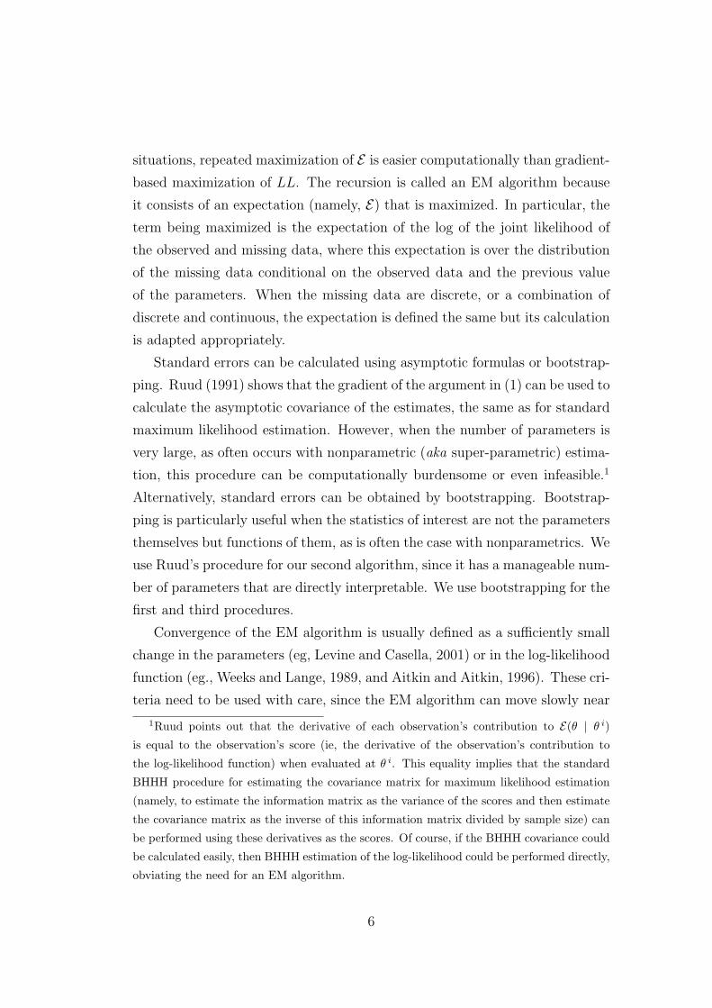
situations, repeated maximization of E is easier computationally than gradient-

based maximization of LL. The recursion is called an EM algorithm because

it consists of an expectation (namely, E) that is maximized. In particular, the

term being maximized is the expectation of the log of the joint likelihood of

the observed and missing data, where this expectation is over the distribution

of the missing data conditional on the observed data and the previous value

of the parameters. When the missing data are discrete, or a combination of

discrete and continuous, the expectation is defined the same but its calculation

is adapted appropriately.

Standard errors can be calculated using asymptotic formulas or bootstrap-

ping. Ruud (1991) shows that the gradient of the argument in (1) can be used to

calculate the asymptotic covariance of the estimates, the same as for standard

maximum likelihood estimation. However, when the number of parameters is

very large, as often occurs with nonparametric (aka super-parametric) estima-

tion, this procedure can be computationally burdensome or even infeasible.1

Alternatively, standard errors can be obtained by bootstrapping. Bootstrap-

ping is particularly useful when the statistics of interest are not the parameters

themselves but functions of them, as is often the case with nonparametrics. We

use Ruud’s procedure for our second algorithm, since it has a manageable num-

ber of parameters that are directly interpretable. We use bootstrapping for the

first and third procedures.

Convergence of the EM algorithm is usually defined as a sufficiently small

change in the parameters (eg, Levine and Casella, 2001) or in the log-likelihood

function (eg., Weeks and Lange, 1989, and Aitkin and Aitkin, 1996). These cri-

teria need to be used with care, since the EM algorithm can move slowly near

1Ruud points out that the derivative of each observation’s contribution to E(θ | θ i)

is equal to the observation’s score (ie, the derivative of the observation’s contribution to

the log-likelihood function) when evaluated at θ i. This equality implies that the standard

BHHH procedure for estimating the covariance matrix for maximum likelihood estimation

(namely, to estimate the information matrix as the variance of the scores and then estimate

the covariance matrix as the inverse of this information matrix divided by sample size) can

be performed using these derivatives as the scores. Of course, if the BHHH covariance could

be calculated easily, then BHHH estimation of the log-likelihood could be performed directly,

obviating the need for an EM algorithm.

6

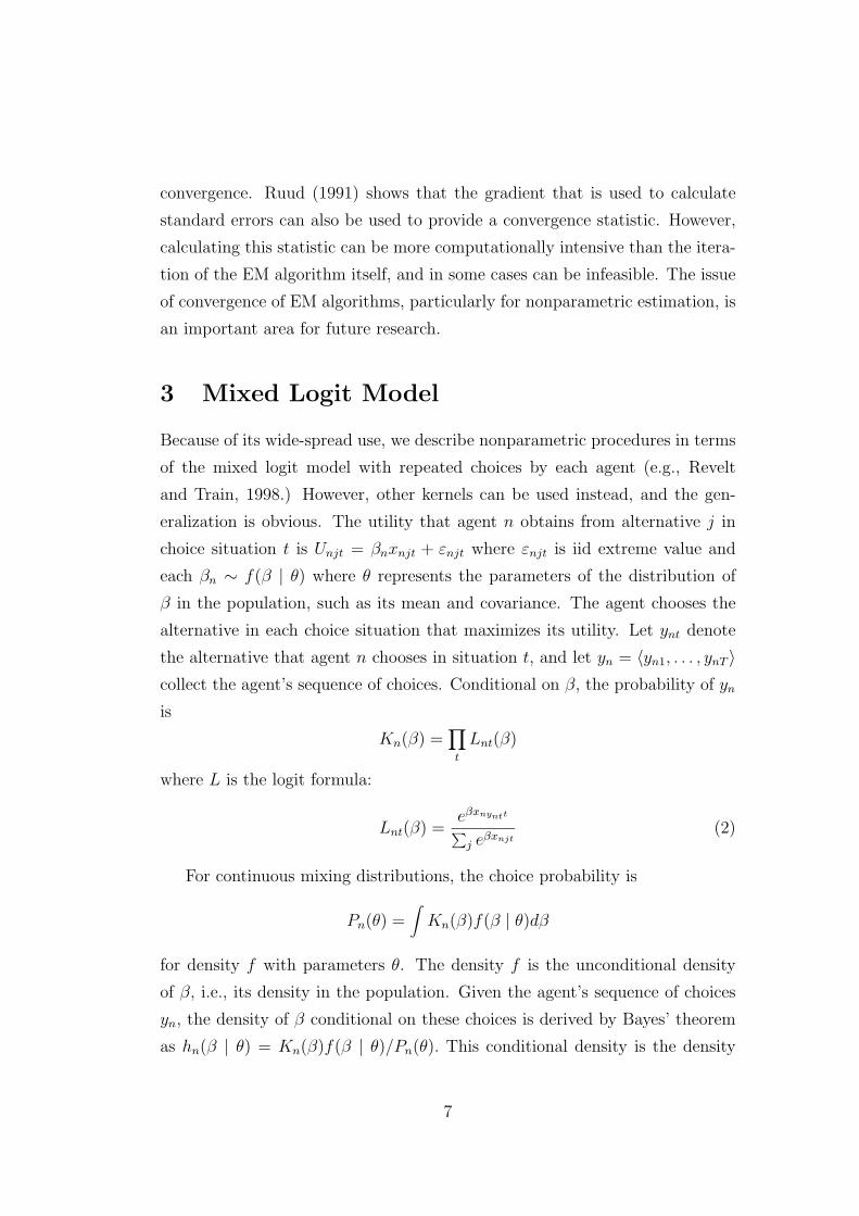
convergence. Ruud (1991) shows that the gradient that is used to calculate

standard errors can also be used to provide a convergence statistic. However,

calculating this statistic can be more computationally intensive than the itera-

tion of the EM algorithm itself, and in some cases can be infeasible. The issue

of convergence of EM algorithms, particularly for nonparametric estimation, is

an important area for future research.

3 Mixed Logit Model

Because of its wide-spread use, we describe nonparametric procedures in terms

of the mixed logit model with repeated choices by each agent (e.g., Revelt

and Train, 1998.) However, other kernels can be used instead, and the gen-

eralization is obvious. The utility that agent n obtains from alternative j in

choice situation t is Unjt = βnxnjt + εnjt where εnjt is iid extreme value and

each βn ∼ f(β | θ) where θ represents the parameters of the distribution of

β in the population, such as its mean and covariance. The agent chooses the

alternative in each choice situation that maximizes its utility. Let ynt denote

the alternative that agent n chooses in situation t, and let yn = 〈yn1, . . . , ynT 〉collect the agent’s sequence of choices. Conditional on β, the probability of yn

is

Kn(β) =∏t

Lnt(β)

where L is the logit formula:

Lnt(β) =eβxnyntt

∑j eβxnjt

(2)

For continuous mixing distributions, the choice probability is

Pn(θ) =∫

Kn(β)f(β | θ)dβ

for density f with parameters θ. The density f is the unconditional density

of β, i.e., its density in the population. Given the agent’s sequence of choices

yn, the density of β conditional on these choices is derived by Bayes’ theorem

as hn(β | θ) = Kn(β)f(β | θ)/Pn(θ). This conditional density is the density

7

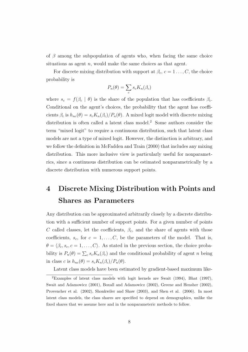
of β among the subpopulation of agents who, when facing the same choice

situations as agent n, would make the same choices as that agent.

For discrete mixing distribution with support at βc, c = 1 . . . , C, the choice

probability is

Pn(θ) =∑

c

scKn(βc)

where sc = f(βc | θ) is the share of the population that has coefficients βc.

Conditional on the agent’s choices, the probability that the agent has coeffi-

cients βc is hnc(θ) = scKn(βc)/Pn(θ). A mixed logit model with discrete mixing

distribution is often called a latent class model.2 Some authors consider the

term “mixed logit” to require a continuous distribution, such that latent class

models are not a type of mixed logit. However, the distinction is arbitrary, and

we follow the definition in McFadden and Train (2000) that includes any mixing

distribution. This more inclusive view is particularly useful for nonparamet-

rics, since a continuous distribution can be estimated nonparametrically by a

discrete distribution with numerous support points.

4 Discrete Mixing Distribution with Points and

Shares as Parameters

Any distribution can be approximated arbitrarily closely by a discrete distribu-

tion with a sufficient number of support points. For a given number of points

C called classes, let the coefficients, βc, and the share of agents with those

coefficients, sc, for c = 1, . . . , C, be the parameters of the model. That is,

θ = 〈βc, sc, c = 1, . . . , C〉. As stated in the previous section, the choice proba-

bility is Pn(θ) =∑

c scKn(βc) and the conditional probability of agent n being

in class c is hnc(θ) = scKn(βc)/Pn(θ).

Latent class models have been estimated by gradient-based maximum like-

2Examples of latent class models with logit kernels are Swait (1994), Bhat (1997),

Swait and Adamowicz (2001), Boxall and Adamowicz (2002), Greene and Hensher (2002),

Provencher et al. (2002), Shonkwiler and Shaw (2003), and Shen et al. (2006). In most

latent class models, the class shares are specified to depend on demographics, unlike the

fixed shares that we assume here and in the nonparameteric methods to follow.

8

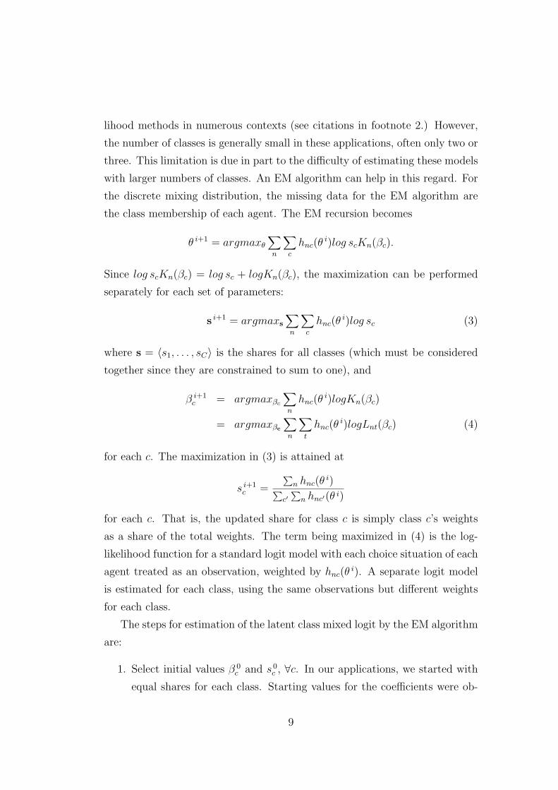
lihood methods in numerous contexts (see citations in footnote 2.) However,

the number of classes is generally small in these applications, often only two or

three. This limitation is due in part to the difficulty of estimating these models

with larger numbers of classes. An EM algorithm can help in this regard. For

the discrete mixing distribution, the missing data for the EM algorithm are

the class membership of each agent. The EM recursion becomes

θ i+1 = argmaxθ

∑n

∑c

hnc(θi)log scKn(βc).

Since log scKn(βc) = log sc + logKn(βc), the maximization can be performed

separately for each set of parameters:

s i+1 = argmaxs

∑n

∑c

hnc(θi)log sc (3)

where s = 〈s1, . . . , sC〉 is the shares for all classes (which must be considered

together since they are constrained to sum to one), and

β i+1c = argmaxβc

∑n

hnc(θi)logKn(βc)

= argmaxβc

∑n

∑t

hnc(θi)logLnt(βc) (4)

for each c. The maximization in (3) is attained at

s i+1c =

∑n hnc(θ

i)∑c′

∑n hnc′(θ i)

for each c. That is, the updated share for class c is simply class c’s weights

as a share of the total weights. The term being maximized in (4) is the log-

likelihood function for a standard logit model with each choice situation of each

agent treated as an observation, weighted by hnc(θi). A separate logit model

is estimated for each class, using the same observations but different weights

for each class.

The steps for estimation of the latent class mixed logit by the EM algorithm

are:

1. Select initial values β 0c and s 0

c , ∀c. In our applications, we started with

equal shares for each class. Starting values for the coefficients were ob-

9

tained by partitioning the sample into C subsamples and estimating a

separate logit on each subsample.3

2. Calculate the weights as

h 0nc ≡ hnc(θ

0) =s 0

c Kn(β 0c )∑

c′ s0c′Kn(β 0

c′).

Note that the denominator is Pn(θ 0).

3. Update the shares as

s 1c =

∑n h 0

nc∑c′

∑n h 0

nc′.

4. Run C standard logits on the data for all choice situations, using weights

h 0nc in the c-th run. Note that these weights are the same for all choice

situations by a given agent. The estimates for run c are the updated

values β 1c .

5. Repeat steps 2-4 to convergence, using the updated parameter values in

lieu of the initial values.

This procedure can be implemented in high-level statistical software pack-

ages, such as stata, that have standard logit estimation routines. An advantage

of this approach is that researchers can estimate a nonparametric mixed logit

using only standard statistical packages. In our application with nearly 10,000

choice situations and seven variables, a model with 20 classes and 159 param-

eters required less than 30 minutes to run using stata. Of course, run times

would be much shorter if the researcher codes the algorithm in matlab or gauss

or, even more-so, Fortran or C.

Standard errors can be calculated by Ruud’s procedure, discussed in section

2 above, using the gradients in (3) and (4). Such calculation is difficult when

3Note that these subsamples do not represent a partitioning of the sample into classes.

The classes are latent and so such partitioning is not possible. Rather, the goal is to obtain

C sets of starting values for the coefficients of the C classes. These starting values must

not be the same for all classes since, if they were the same, the algorithm would perform

the same calculations for each class and return for all classes the same shares and up-dated

estimates in each iteration. An easy way to obtain C different sets of starting values is to

divide the sample into C groups and estimate a logit on each group.

10

using high-level packages, since these packages do not output the gradients that

are utilized internally. Alternatively, the standard errors can be calculated by

bootstrap. If the model contains a large number of classes, then summary

statistics can be more relevant than each sc and βc. Bootstrapping allows

the standard errors for these summary statistics to be calculated straightfor-

wardly. By contrast, if standard errors are calculated for the parameters using

asymptotic formulas, the application of derivative formulas is required to ob-

tain standard errors for the summary statistics. Stata contains a bootstrap

command.

5 Discrete Mixture of Continous Distributions

Any continuous distribution can be approximated by a discrete mixture of nor-

mal distributions. This approximation is used by Fosgerau and Hess (2007) for

one of their nonparametric mixed logits. With C normals, the parameters are

the share sc, mean bc, and covariance Vc of each normal. To provide greater

structure in the approximating distribution, the utility coefficients can be speci-

fied as transformations of underlying latent normal terms, as Train and Sonnier

(2005) utilized in Bayesians estimation with normals. For example, exponen-

tiating the normal terms gives log-normally distributed coefficients. However,

since the generalization is obvious and yet notationally cumbersome, we main-

tain in the current description that the coefficients are normally distributed

without transformation.

The choice probability is

Pn(θ) =∑

c

sc

∫Kn(β)φ(β | bc, Vc)dβ.

where φ(β | bc, Vc) is the normal density with mean bc and variance Vc. This

probability is simulated by taking R draws from each normal distribution for

each agent, labeled βncr for draw r from normal c for agent n, and averaging

over the draws and classes:

Pn(θ) =∑

c

sc

∑r

Kn(βncr)/R

11

The missing data for the EM algorithm are the class membership and value

of β for each agent. Conditional on the agent’s choices, the probability-density

of β and class c is

hnc(β | θ) = scφ(β | bc, Vc)Kn(β)/Pn(θ). (5)

The expectation in the EM algorithm is

E(θ | θ i) =∑n

∑c

∫hnc(β | θ i)log [sc φ(β | bc, Vc)Kn(β)]dβ.

Substituting (5) and rearranging gives

E(θ | θ i) =∑n

∑c

∫[scKn(β)/Pn(θ i)]log [sc φ(β | bc, Vc)Kn(β)]φ(β | bc, Vc)dβ.

The integrals over densities φ(·) are approximated by simulation using the same

draws as for P above. The simulated expectation is:

E(θ | θ i) =∑n

∑c

∑r

h incr log [sc φ(βncr | bc, Vc)Kn(βncr)]/R

where the weights are defined by h inrc = scK(βnrc)/Pn(θ i). Note that Kn(βncr)

does not depend on the parameters: a change in the parameters changes the

density of βncr, which is captured in φ(βncr | bc, Vc), but does not change the

evaluation of Kn(βncr) for any particular value of βncr. Kn(βncr) therefore drops

out of the log (but not the weights) for maximization of E with respect to the

parameters. The recursion becomes

s i+1 = argmaxs

∑n

∑c

∑r

h incr log sc (6)

and

〈bc, Vc〉 i+1 = argmaxbc,Vc

∑n

∑r

h incr log φ(βncr | bc, Vc) (7)

for each c. The maximization in (6) is satisfied by

s i+1c =

∑n

∑r h i

ncr∑c′

∑n

∑r h i

nc′r

which is just the share of weights in class c. Recursion (7) is the maximum

likelihood estimator for a sample of weighted draws from a normal distribution.

12

The ML estimator of the mean and covariance of a normal distribution based on

weighted draws from that distribution is, of course, the mean and covariance of

the weighted draws. The mean and covariance of the c-th normal distribution

is updated simply by taking the mean and covariance of the N · R draws βncr

with weights h incr ∀n, r. No logit estimation is required for this algorithm, only

the calculation of logit probabilities for the weights.

The steps are as follows:

1. Select initial values s 0c , b 0

c , V 0c , c = 1, . . . , C. In our application with

two normals, we started with equal shares, a vector of zeros and ones,

respectively, for the means, and covariances with large diagonal elements

and zero off-diagonal elements.

2. Take R draws from each normal for each agent, using mean b 0c and co-

variance V 0c for the c-th normal. Label the r-th draw for agent n from

normal c as β 0ncr.

3. Calculate the weight for each draw from each normal for each agent as

h 0ncr = scK(β 0

nrc)/Pn(θ 0).

4. Update the shares as

s 1c =

∑n

∑r h 0

ncr∑c′

∑n

∑r h 0

nc′r.

5. Update the mean and covariances as

b 1c =

∑n

∑r h 0

ncrβ0ncr∑

n

∑r h 0

ncr

and

V 1c =

∑n

∑r h 0

ncr[(β0ncr − b 1

c )(β 0ncr − b 1

c )′]∑n

∑r h 0

ncr

.

6. Repeat steps 2-5 until convergence, using the updated values in each

iteration.

Standard errors are readily calculated using the gradient of (6) and (7), as

described by Ruud (1991). Train (2007) adapts Ruud’s formulas for application

to a normal mixing distribution.

13

As mentioned above, the procedure can be readily generalized to allow the

coefficients that enter utility to be transformations of β, such that the distribu-

tion of coefficients is, e.g., a discrete mixture of lognormal or truncated normal

distributions. Utility is expressed as Unjt = T (βn)xnjt +εnjt for transformation

T (·) that depends only on the value of βn, which is itself distributed as a dis-

crete mixture of normals with mean bc and covariance Vc in class c. The logit

formula in equation 2 is adapted appropriately as:

Lnt(β) =eT (β)xnyntt

∑j eT (β)xnjt

All other formulas remain the same. In the iterative process, the transformation

affects only the weights h inrc ∀n, r, c since these weights depend on the logit

formula. However, given the weights, the recursion still calculates the weighted

mean and covariance of the draws of (untransformed) β from each normal to

update bc and Vc ∀c.

6 Discrete Distribution with Fixed Points and

Shares Treated as Parameters

The procedure in section 4 requires repeated estimation of standard logits. The

procedure in section 5 does not require logit estimation, but requires repeated

calculation of the logit formula. The procedure in this section requires neither.

The logit probabilities are calculated once for the fixed points, and then all

iterations use these calculated values. As a result, a very large number of fixed

points (e.g, hundreds of thousands) can be specified while still maintaining

relatively fast estimation. The drawback of this procedure, which we explain

more in discussion of the applications, is that we have found summary statistics,

such as mean coefficients, to be highly sensitive to the specification of the range

of fixed points.

Let the mixing distribution be approximated by a discrete distribution with

share sc at point βc for c = 1, . . . , C, as in section 4. However, we now consider

βc∀c to be specified by the researcher instead of estimated. The parameters of

the model are the shares sc,∀c. Bajari et al. (2007) utilize this specification

14

for their nonparametric estimation of a mixed logit. The fixed points can be

specified as a full grid over the parameter space, a sparse grid, a Halton or

other sequence of points, or drawn randomly from a generating distribution.

To maintain the same nomenclature as in section 4, each point is called a class,

with C classes in total. The choice probabilities and conditional probabilities

of class membership are the same as in section 4. The EM recursion is also the

same, except that now the parameters θ = s do not include the βc’s:

s i+1 = argmaxs

∑n

∑c

hnc(si)log scKn(βc).

However, since the βc’s are fixed rather than parameters, Kn(βc) drops out.

The recursion becomes simply

s i+1 = argmaxs

∑n

∑c

hnc(si)log sc,

which is satisfied by

s i+1c =

∑n hnc(s

i)∑c′

∑n hnc′(s i)

.

The algorithm is implemented by the following steps:

1. Select the fixed points βc,∀c.

2. Calculate the logit kernel, Kn(βc), for each agent at each point.

3. Specify initial shares s 0c ,∀c. In applications, we have used equal shares

as starting values.

4. Calculate weights for each agent at each point:

h 0nc =

s 0c Kn(βc)∑

c′ s 0c′Kn(βc′)

.

5. Update the share at each point as:

s 1c =

∑n h 0

nc∑c′

∑n h 0

nc′.

6. Repeat steps 4 and 5 until convergence, using the updated shares.

As with the method in section 4, standard errors for the parameters and sum-

mary statistics are most readily obtained by bootstrap.

15

7 Application

We apply the methods to data on consumer’s choice among alternative-fueled

vehicles in stated-preference experiments. The data were developed in a project

for the National Renewable Energy Laboratory and are described in detail by

Baumgartner et al. (2007). The sample consists of people who live in the 10-

county area of Southern California, are at least 18 years old, and had purchased

a new vehicle in the last three years. Each respondent was presented with 10

choice experiments. In each experiment, the respondent was offered a choice

among three alternatives: the conventional-fuel vehicle (CV) that the respon-

dent had recently purchased and two alternative-fueled vehicles (AV’s) with

specified attributes. The attributes represent relevant features of hydrogen ve-

hicles, but the respondents were not told that the alternative fuel was hydrogen

so as to avoid any preconceptions that respondents might have developed with

respect to hydrogen vehicles. The attributes included in the experiments are:

• Fuel cost (FC), expressed as percent difference from the CV. In estima-

tion, the attribute is scaled as a share, such that fuel costs of 50 percent

less than the conventional vehicle enters as -0.5, and 50 percent more

enters as 0.5.

• Purchase price (PP), expressed as percent difference from the CV, scaled

analogously to fuel cost when entering the model.

• Driving radius (DR): the farthest distance from home that one is able to

travel and then return, starting on a full tank of fuel. As defined, driving

radius is one-half of the vehicle’s range. In the estimated models, DR is

scaled in hundreds of miles.

• Convenient medium distance destinations (CMDD): the percent of des-

tinations within the driving radius that “require no advanced planning

because you can refuel along the way or at your destination” as opposed

to destinations that “require refueling (or at least estimating whether

you have enough fuel) before you leave to be sure you can make the

round-trip.” This attribute reflects the distribution of potential destina-

tions and refueling stations within the driving radius, recognizing that

16

the tank will not always be full when starting. In the estimated models,

it is entered as a share, such that, e.g., 50 percent enters as 0.50.

• Possible long distance destinations (PLDD): the percent of destinations

beyond the driving radius that are possible to reach because refueling

is possible, as opposed to destinations that cannot be reached due to

limited station coverage. This attribute reflects the extent of refueling

stations outside the driving radius and their proximity to potential driv-

ing destinations. It enters the models scaled analogously to CMDD.

• Extra time to local stations (ETLS): additional one-way travel time be-

yond the time typically required to find a conventional fuel station re-

quired to get to an alternative fuel station in the local area. ETLS was

defined as having values of 0, 3 and 10 minutes in the experiments; how-

ever, in preliminary analysis, it was found that respondents considered

3 minutes to be no inconvenience (i.e., equivalent to 0 minutes). In the

estimated models therefore, we enter a dummy variable for ETLS being

10 or not, rather than ETLS itself.

In the experiments, the CV that the respondent had purchased was described

as having a driving radius of 200 miles, CMDD and PLDD equal to 100 percent,

and, by definition, ETLS, FC and PP of 0. For the AV’s, several levels were

specified for each attribute4 and 480 distinct experiments (i.e., combination of

levels) were generated based on the efficient choice designs of Zwerina et al.

(2005). The 480 experiments were combined randomly into 48 sets with 10

experiments in each. Each respondent was randomly assigned to one of the 48

sets.

In each experiment, the respondent was asked to identify the best and

worst of the three alternatives, thereby providing a ranking of the three. In

estimation, the ranking probabilities were specified in the standard way, using

the “exploded logit” formula conditional on the coefficients (Luce and Suppes,

1965, as discussed in Train, 2003, section 7.3.1). That is, the probability of the

4As follows: FC: -0.5, 0, 0.5. PP: -0.15, 0. 0.15. DR: 200, 150, 100. CMDD: 1, 0.9, 0.5,

0. PLDD: 1, 0.9, 0.5, 0. ETLS: 0, 3, 10.

17

ranking is the logit probability of the first choice from the three alternatives

in the experiment, times the logit probability for the second choice from the

two remaining alternatives. With random coefficients, this kernel probability

is mixed over the distribution of coefficients. The specification is equivalent to

the mixed logit model described in section 4 above, with the repeated choices

being the first and second choice of the respondent in each of the ten choice

situations (for T = 20 total choices per respondent, if the respondent answered

all of them.) A total of 510 respondents completed the survey, of which 508

answered at least some of the choice experiments. These 508 respondents are

used in our estimation, generating a total of 9844 choices including first and

second choices.

Table 1 presents the results of a standard logit model estimated on these

data. All coefficients take the expected signs and are highly significant. The

estimates indicate that respondents consider a percent increase in purchase

price to be equivalent to about a half-percent increase in fuel cost. An increase

in the percent of long distance locations that can be reached is estimated to

be more valuable than an increase in the percent of medium distant locations

that can be reached without needing to think about refueling. The last variable

is a dummy identifying the CV that the respondent purchased. Its negative

coefficient indicates that respondents would prefer an AV over a CV if the AV

had the same price, fuel cost, 200 mile radius, 100 percent of medium distance

locations accessible without needing to thinking about refueling, 100 percent of

long distance destinations accessible, and equivalent time to a local refueling

station. This preference can reflect respondents’ value of the reduced emis-

sions of the AV’s, which were described to respondents as part of the general

description of the choice experiments (and held constant over the experiments.)

Alternatively, the estimated coefficient could reflect a tendency for respondents

to choose the AV’s because they thought they were supposed to.

Table 2 gives the results of a mixed logit with independent, normally dis-

tributed coefficients, using 100 standard Halton draws for simulation. The

estimated means have the same signs and similar relative magnitudes as in

the standard logit. The standard deviations are large relative to the means

and highly significant, indicating considerable differences in preferences over

18

respondents. Of course, the normal distribution implies that a portion of re-

spondents dislike positive attributes and like positive attributes.

Alternative models were estimated (not shown) that allowed the normally

distributed coefficients to be correlated. The estimated correlations were found

to be significant, with reasonable patterns. For example, the coefficients for

fuel cost and purchase price are positively correlated, as are the coefficients of

CMPP and PLDD. However, the shares with wrong signs was higher than in

the models without correlation. Models were also estimated with lognormal

coefficients and truncated normal distributions for the signed coefficients (i.e.,

for all the coefficients except that on the CV dummy which could logically take

either sign.) These specifications fit considerably worse than the model with a

normal distribution.

We applied each of the three nonparametric methods described above. We

discuss each in turn.

7.1 Discrete Distribution with estimated shares and co-

efficients

For the latent class model in section 4, the researcher specifies the number of

classes C and estimates the share sc and coefficients βc for each class. We coded

the EM algorithm into stata, which has a logit estimation procedure (clogit).

In each iteration, a logit model is estimated for each of the C classes using the

same observations but different weights for each class. We utilized 50 iterations

in each run. Fewer iterations would have probably been sufficient, since the

log-likelihood function rose less than one-twentieth of one percent during the

last ten iterations combined for all the models that we estimated with this

method. However, as mentioned in section 2, it is advisable to be cautious in

assessing convergence since EM algorithms can move slowly near convergence.

Run time is proportional to the number of classes, requiring about 1.5 minutes

per class (for all 50 iterations) on our standard-issue PC. For example, the

model with 10 classes took about 15 minutes to run. As stated in section 4,

run times would be lower if the procedure were coded into lower-level languages

than stata.

19

The selection of C can be based on information criteria, such as the AIC

or BIC,5 and on examination of the reasonableness of the results with different

numbers of classes. Table 3 gives the log-likelihood value, AIC, and BIC for

the model using various numbers of classes. The AIC is lowest (best) with 25

classes and the BIC, which penalizes extra parameters more heavily than the

AIC, is lowest with 8 classes.

Table 4 gives the estimated model with 8 classes. The estimates for the

model with 25 classes, which is best by the AIC, are not given for the sake

of brevity. The largest of the 8 classes is the last one with 25 percent. Inter-

estingly, this class has a large, positive coefficient for CV, unlike all the other

classes. This class consists of people who prefer their CV over AV’s even when

the AV has the same attributes – perhaps because of the uncertainty associated

with new technologies. Other distinguishing features of classes are evident. For

example, class 3 cares far more about purchase price than the other classes,

while class 1 places more importance on fuel cost than the other classes.

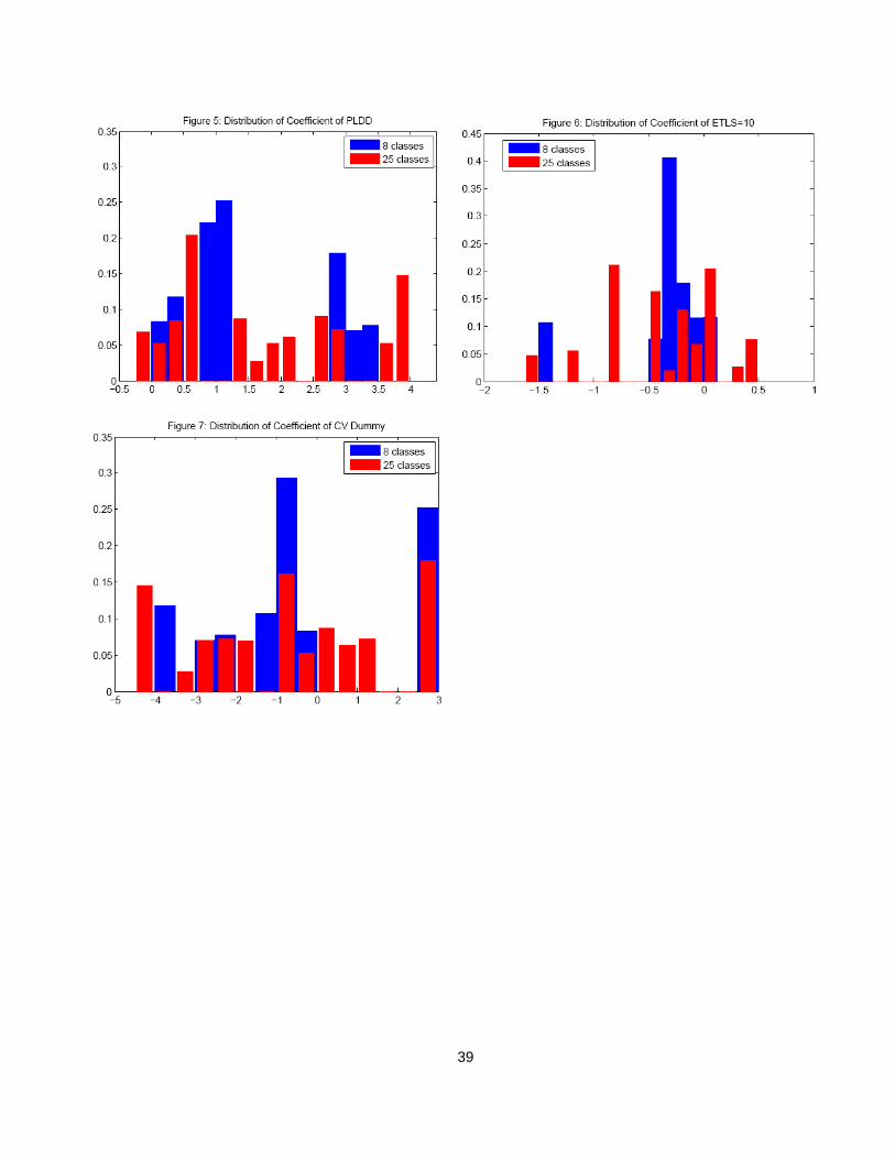
Figures 1-7 give the histogram for each of the seven coefficients for the

models with 8 and 25 classes. There are fewer bars than classes in these

histograms because the histograms place the values in bins, and more than one

class can fall into a bin. The distributions are fairly similar, with the 25-class

distribution being less “peaked” than that from the 8-class model, as expected.

Standard errors were calculated by bootstrap, using 20 bootstrap samples.

As expected, the standard errors for sc and βc ∀c are fairly large, while the

standard errors for relevant summary statistics, such as means, are relatively

small. Table 5 gives estimates and standard errors for class 1’s share and

coefficients, which is exemplary of all classes, and for the mean and standard

deviations of the coefficients over all classes, based on the model with 8 classes.

As the table shows, the standard errors for the class 1 parameters are large. It

is not clear, however, what exactly is meant by a standard error for class “1”,

since the class labeling is arbitrary. Suppose, as an extreme but illustrative

example, that two different bootstrap samples give the same estimates for two

5The Akaike Information Criterion (AIC) is −2LL+2K where LL is the value of the log-

likelihood and K is the number of parameters. The Bayesian, also called Schwartz, criterion

(BIC) is −2LL + log(N)K where N is sample size, in our case 508.

20

classes but with their order changed (i.e., the estimates for class 1 becoming the

estimates for class 2, and vice versa). In this case, the bootstrapped standard

errors for the parameters for both classes rise even though the model for these

two classes together is exactly the same. Summary statistics of course avoid

this issue. All but one of the means are statistically significant, with the CV

dummy obtaining the only insignificant mean. All of the standard deviations

are significantly different from zero.

The means and standard deviations are somewhat smaller in magnitude

than those obtained with normal mixing distribution (Table 2). However, this

difference disappears for the the model with 25 classes, which gives means and

standard devaitions that are somewhat larger than the model with 8 classes

and similar to the model with normal mixing distribution. The similarity indi-

cates, as we find below for the other procedures as well, that the nonparametric

methods provide greater flexibility in the shape of the distribution while main-

taining about the same means and standard deviations.

With unconstrained latent class estimation, estimated coefficients can take

the wrong sign due, if nothing else, to sampling variance. In the model with

8 classes, three of the 56 coefficients have the wrong sign. Each of these three

is relatively small in magnitude and is not significantly different from zero.

With more classes, the number of wrong signs increases, as one would expect.

With 25 classes, 22 of the 175 coefficients had the wrong sign. There are

two ways that incorrect signs could be avoided. First, the model could be

reestimated with the variables with wrong signs for a given class removed

for that class. Alternatively, the logit estimation in each iteration for each

class could incorporate inequality constraints on the signed coefficients. Such

constraints cannot be specified within the clogit proc in stata; however, they

are feasible in matlab or gauss using their constrained optimization routines.

This issue is a potentially fruitful area for further analysis.

7.2 Discrete Mixture of Continuous Distributions

We estimated a model using the method in section 5, with a discrete mixture of

two multivariate normal distributions. The results are given in Table 6, using

21

for simulation 100 standard Halton draws for each normal for each respondent.

Standard errors are calculated by the method in Train (2007) which is easier

than bootstrapping for this type of model. Recall that each iteration consists

of taking draws from the two normals using the previous values of their mean

and covariance, calculating weights for each draw, and calculating the mean

and covariance of the weighted draws, which then become the new values. We

coded the procedure in matlab since the iterations consist only of arithmetic,

for which stata is particularly slow. In matlab, estimation of the model with

two normals and 71 parameters (7 means, 7 variances, and 21 off-diagonal

covariances for each normal, plus one share, with the other share being 1 minus

the first) took only 2 minutes and 42 seconds, including the calculation of the

standard errors.

The two classes are essentially the same size. We used equal shares for

starting values; however, the share for class 1 dropped to 37 percent during

iteration before rising back to its estimated value of 49.6 percent. Class 2 has a

positive coefficient for the CV dummy, while class 1 has a negative coefficient.

This result mirrors the finding in subsection 7.1 that a share of the population

prefer a CV over an AV even when the AV has the same attributes as the CV.

Class 2 has much larger (in magnitude) coefficients than class 1 for purchase

price and the dummy for 10 minutes extra to drive to a refueling station. Class

2 can be characterized as people who are very unlikely to buy an AV (at least

in the early stages of AV introduction), because of their positive CV dummy

as well as the fact that AV’s will initially cost more than CV’s and will require

longer drives to refueling stations, both of which attributes these people have

strong preferences against. In contrast, class 1 consists of people who prefer

AV’s, all else equal, place far less weight on purchase price and time spent

driving to a refueling station, and place far greater positive value on driving

radius, CMDD, and PMDD.

The off-diagonal covariance terms are not given in Table 6 for the sake of

brevity. For class 1, the largest correlations are between:

• driving radius and CMDD. The correlation is -0.80, indicating that peo-

ple in this class who place a greater-than-average importance on driving

radius tend to place a less-than-average importance on the share of des-

22

tinations within that radius that can be reached without thinking about

refueling.

• fuel cost and purchase price, 0.65, indicating that people who care greatly

about one of these costs also tend to care greatly about the other.

• the dummies for CV and 10 minutes extra time to a refueling station,

-0.60, indicating that people who tend to like AV’s more than average

(i.e. have a more negative coefficient for the CV dummy) also tend to

place less importance on extra refueling time (i.e, have a less negative

coefficient for the extra time dummy.)

For class two, the largest correlations are between:

• extra driving time and fuel cost, 0.72, indicating that respondents in

this class who have greater-than-average dislike for driving time 10 extra

minutes to a refueling station also tend to have a greater-than-average

dislike of higher fuel costs.

• extra driving time and driving radius, -0.68, indicating that respondents

who dislike the extra driving time more than average also tend to place

a greater-than-average importance on driving radius.

• extra driving time and CMDD, 0.54, indicating that respondents who

have a greater-than average dislike for extra driving time also tend to

put a smaller-than-average value on CMDD.

• driving radius and fuel cost, -0.54, indicating that people with greater-

than-average value of a wider driving radius also tend to have greater-

than-average concern about fuel cost.

The estimates for each class can be used to calculate the oveall means and

standard deviations for the population. The means are very similar to those in

Table 2 for a model with one normal distribution. The standard deviations are

also similar, except for CDDD which obtains a considerably larger standard

deviation in the model with two normals than one.

23

We estimated models with the utility coefficients being transformations of

β, such that the distribution of coefficients is a discrete mixture of lognor-

mal, and truncated normal, distributions. These models obtained a lower LL

than that in Table 6 but had the advantage, of course, of correctly signed util-

ity coefficients for the entire population. The relative fit is case-specific. In

Train and Sonnier’s (2005) application, for example, lognormals and truncated

normals gave a considerably higher LL than normals. Such transformations

are, therefore, worth examining when approximating the mixing distribution

nonparametrically through a discrete mixture of normals.

7.3 Discrete Distribution with Fixed Coefficients

This third nonparametric procedure is the easiest conceptually and compu-

tationally. As with the previous procedure, we coded it into matlab since it

requires only arithmetic. The key element of this procedure, which we discuss

in more detail below, is the specification of the fixed points. We determined the

maximum and minimum for each coefficient, using the estimation results from

section 7.1 above combined with sign constraints. (That is, we set the maxi-

mum of the price coefficient at 0, even though the latent class models in 7.1

contained some classes with positive price coefficients.) One advantage of this

approach is that sign constraints are easy to implement, simply by maintaining

the constraints in the specification of the fixed points. We then estimated mod-

els with two alternative ways of defining the points between the minimum and

maximum for each coefficient: (1) complete grids, and (2) Halton sequences.

The complete grids were created from equally spaced points in each dimension

between the minimum and maximum for that dimension (with the endpoints

included as points.)6 We specified two complete grids and estimated the model

on each. For one of the complete grids, we used 5 values for each of the 7

coefficients, for a total of 57 = 78, 125 values of β in the complete grid. For

6We included zero as a possible value for each signed coefficients because in SP experi-

ments, each respondent might ignore one or more attributes, which is equivalent to giving

them utility coefficients of zero. As the results given below indicate, each of the signed coef-

ficients is estimated to have a non-neglible share at zero, indicating that some respondents

are estimated to have ignored each attribute.

24

another grid, we used 6 values for 6 of the coefficients and 5 for the remaining

coefficient (the CV coefficient), for 233,280 points in total. Estimation was fast

with both of these grids: taking 11 minutes for the grid of 78,125 points and

31 minutes for the grid with 233,280 points. We did not attempt any finer

grids because of memory constraints, which we could have, but did not, code

around.7 A Halton sequence of 10,000 points was created in the standard way

(Halton, 1960; as described by Bhat, 2001, and Train, 2003, section 9.3.3),

using the seven primes between 2 and 17, inclusive, for the 7 dimensions.8 Run

time with 10,000 Halton points as commensurately faster that the complete

grids with more points, clocking in at 2 minutes, 9 seconds.

Table 7 gives summary statistics for the models estimated on the three

different set of points, using the same maximum and minimum values for each

set. The means and standard deviations are very similar across the three

models. The complete grids provide considerably better fit than the Halton

sequence, which might be expected since the complete grids have many more

points. The complete grid with 233,280 points obtains only a very slightly

better fit than the complete grid with 78,125 points. The means and standard

deviations are also fairly similar to those obtained for the model with a normal

mixing distribution (Table 2). The one main difference is a larger standard

deviation for the CMDD coefficient, which was also found for the model with

two normals, discussed above. Again, this similarity implies that the procedure

provides greater flexibility in the shape of the distribution while obtaining

similar over-all means and standard deviations.

Figures 8-14 give the frequency distribution for each coefficient based on

7The capacity of matlab’s memory map was reached with 233,280 points, which translated

into about 120 million double-precision numbers since the logit kernel is calculated and held

for each agent at each point. More points can be used in estimation by writing these values

to a file and reading them into memory in blocks at each iteration.8In maximum simulated likelihood, usually a much smaller number of Halton points are

used for each observation, since simulation noise cancels out when averaging over obser-

vations. For the current use, the same Halton points are used for each person, and the

points are intended to “cover” the parameter space. An potentially interesting extension

is to examine the implications of using a different set of points for each person within the

nonparametric EM algorithm.

25

the finer grid. Figures 15 and 16 show the joint distribution for selected pairs

of coefficients, namely, fuel cost and driving radius, and CMDD and PLDD.

An advantage of the full grid is that is it very easy to obtain any specific

marginal and/or conditional distribution implied by the joint distribution over

the grid points. For example, Figure 17 shows the distribution of the fuel

cost coefficient conditional on the CV coefficient being positive (i.e., prefer

an CV to a comparable AV) and the price coefficients being less than -4.8

(indicating more-than-average concern about price), and marginal over all the

other coefficients.

Given the wealth of information that is obtained with this procedure, and

the speed of its estimation, this form of nonparametric estimation seems partic-

ularly attractive. There is, however, an important issue that requires attention.

In particular, we found that the summary statistics changed considerably when

the range of the parameter space was changed. Table 8 illustrates the issue,

giving the estimated means and standard deviations of the coefficients under

alternative ranges for the coefficients (but the same number of points within

the range.) The first column is the model already presented in Table 7, using

the ranges that we originally specified. The second column gives results for

a model with the maxima and minima doubled. Note that for all the signed

coefficients (i.e., all except the coefficient of the CV dummy), this change in-

creased the range in one direction only. In all cases, the estimated means and

standard deviations rose in magnitude (though less than double.) This result

would perhaps not be a problem if ratios remained stable. However, column

3 gives results for a model in which the range of the fuel cost coefficient is

doubled and the other coefficients retain their original ranges. The mean of

the fuel cost coefficient rises, while the others do not (or not nearly as much.)9

There are several ways that this issue could be addressed. One procedure

is to select the range that provides the highest LL. By this criterion, our

9A referee suggested that these discrepancies might have arisen because the range was

originally set by the maxima and minima from the latent class models in section 7.1, which

contained relatively few classes and consequently might have under-represented the true

spread of the coefficients. This explanation is consistent with our finding, stated in the next

paragraph, that increasing the range raised the log-likelihood.

26

original ranges would be doubled for all coefficients, since the LL is slightly

higher with the wider ranges. A second procedure is to specify ranges in the

way we originally did, namely, by first estimating a latent class model and then

using the ranges implied by the estimated classes in a model with fixed points.

A third procedure is for the researcher to place a prior distribution on the

parameter values, and incorporate this prior in estimation. Of course, choosing

a range is equivalent to placing a prior that is constant within the range and

zero outside the range. Specifying a prior involves the same decisions and

possible arbitrariness, though stated differently and with greater generality,

as specifying the range. In any case, this form of nonparametrics based on

fixed points seems sufficiently promising to warrant further research on the

appropriate specification of the points.

27

References

Aitkin, M. and I. Aitkin (1996), ‘A hybrid EM/Gauss-Newton algorithm for

maximum likelihood in mixture distributions’, Statistics and Computing

6, 127–130.

Bajari, P., J. Fox and S. Ryan (2007), ‘Linear regression estimation of discrete

choice models with nonparametric distributions of random coefficients’,

American Economic Review 97(2), 459–463.

Baumgartner, R., E. Rambo and A. Goett (2007), ‘Discrete choice analysis for

hydrogen vehicles’, Report to the National Renewable Eenergy Labora-

tory, PA Consulting Group, Madison WI.

Bhat, C. (1997), ‘An endogenous segmentation mode choice model with an

application to intercity travel’, Transportation Science 31, 34–48.

Bhat, C. (1998), ‘Accommodating variations in responsiveness to level-of-

service variables in travel mode choice models’, Transportation Research

A 32, 455–507.

Bhat, C. (2000), ‘Incorporating observed and unobserved heterogeneity in ur-

ban work mode choice modeling’, Transportation Science 34, 228–238.

Bhat, C. (2001), ‘Quasi-random maximum simulated likelihood estimation of

the mixed multinomial logit model’, Transportation Research B 35, 677–

693.

Boxall, P. and W. Adamowicz (2002), ‘Understanding heterogeneous prefer-

ences in random utility models: A latent class approach’, Environmental

and Resource Economics 23, 421–446.

Boyles, R. (1983), ‘On the convergence of the EM algorithm’, Journal of the

Royal Statistical Society B 45, 47–50.

Dempster, A., N. Laird and D. Rubin (1977), ‘Maximum likelihood from in-

complete data via the EM algorithm’, Journal of the Royal Statistical

Society B 39, 1–38.

28

Fosgerau, F. and S. Hess (2007), ‘Competing methods for representing ran-

dom taste heterogeneity in discrete choice models’, Working paper, Danish

Transport Research Institute, Copenhagen.

Greene, W. and D. Hensher (2002), ‘A latent class model for discrete choice

analysis: Contrasts with mixed logit’, working paper ITS-WP-02-08, In-

stitute of Transport Studies, University of Sydney and Monash University.

Halton, J. (1960), ‘On the efficiency of evaluating certian quasi-random se-

quences of points in evaluating multi-dimensional integrals’, Numerische

Mathematik 2, 84–90.

Hensher, D. (2006), ‘Joint estimation of process and outcome in choice experi-

ments involving attribute framing’, working paper, Institute of Transport

and Logistic Studies, University of Sydney.

Hensher, D. and W. Greeene (2003), ‘Mixed logit models: State of practice’,

Transportation 30(2), 133–176.

Levine, R. and G. Casella (2001), ‘Implementation of the monte carlo EM

algorithm’, Journal of Computational and Graphical Statistics 10, 422–

439.

Luce, R. D. and P. Suppes (1965), Preferences, utility, and subjective proba-

bility, in R. D.Luce, R.Bush and E.Galanter, eds, ‘Handbook of Mathe-

matical Psychology’, John Wiley and Sons, New York, pp. 249–410.

McFadden, D. and K. Train (2000), ‘Mixed MNL models of discrete response’,

Journal of Applied Econometrics 15, 447–470.

McLachlan, G. and T. Krishnan (1997), The EM Algorithm and Extensions,

Wiley, New York.

Provencher, B., K. Baerenklau and R. Bishop (2002), ‘A finite mixture logit

model of recreational angling with serially correlated random utility’,

American Journal of Agricultural Economics 84(4), 1066–1075.

29

Revelt, D. and K. Train (1998), ‘Mixed logit with repeated choices’, Review of

Economics and Statistics 80, 647–657.

Ruud, P. (1991), ‘Extensions of estimation methods using the em algorithm’,

Journal of Econometrics 49, 305–341.

Shen, J., Y. Sakata and Y. Hashimoto (2006), ‘A comparison between latent

class model and mixed logit model for transport mode choice: Evidences

from two datasets of japan’, discussion paper 06-05, Graduate School of

Economics, Osaka University.

Shonkwiler, J. and D. Shaw (2003), A finite mixture approach to analyzing

income effects in random utility models, in N.Hanley, ed., ‘The New Eco-

nomics of Outdoor Recreation’, Edward Elgar, pp. 268–279.

Swait, J. (1994), ‘A structural equation model of latent segmentation and prod-

uct choice for cross-sectional revealed preference choice data’, Journal of

Retailing and Consumer Services 1(2), 77–89.

Swait, J. and W. Adamowicz (2001), ‘The influence of task complexity on

consumer choice: A latent class model of decision strategy switching’,

Journal of Consumer Research 28, 135–148.

Train, K. (1998), ‘Recreation demand models with taste variation’, Land Eco-

nomics 74, 230–239.

Train, K. (2003), Discrete Choice Methods with Simulation, Cambridge Uni-

versity Press, New York.

Train, K. (2007), ‘A recursive estimator for random coefficient models’, working

paper, Department of Economics, U. of California, Berkeley.

Train, K. and G. Sonnier (2005), Mixed logit with bounded distributions of cor-

related partworths, in R.Scarpa and A.Alberini, eds, ‘Applications of Sim-

ulation Methods in Environmental and Resource Economics’, Springer,

Dordrecht, pp. 117–134.

30

Weeks, D. and K. Lange (1989), ‘Trials, tribulations, and triumphs of the

EM algorithm in pegigree analysis’, Journal of Mathematics Applied in

Medicine and Biology 6, 209–232.

Wu, C. (1983), ‘On the convergence properties of the EM algorithm’, Annals

of Statistics 11, 95–103.

Zwerina, K., J. Huber and W. Kuhfeld (2005), ‘A general method

for constructing efficient choice designs’, SAS Institute report at

http://support.sas.com/techsup/technote/ts722e.pdf.

31

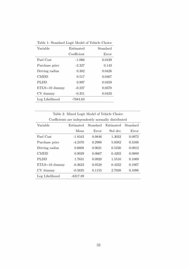
Table 1: Standard Logit Model of Vehicle Choice

Variable Estimated Standard

Coefficient Error

Fuel Cost -1.066 0.0439

Purchase price -2.327 0.143

Driving radius 0.382 0.0426

CMDD 0.517 0.0467

PLDD 0.997 0.0459

ETLS=10 dummy -0.227 0.0370

CV dummy -0.351 0.0433

Log Likelihood -7884.63

Table 2: Mixed Logit Model of Vehicle Choice

Coefficients are independently normally distributed

Variable Estimated Standard Estimated Standard

Mean Error Std dev Error

Fuel Cost -1.8342 0.0846 1.3033 0.0972

Purchase price -4.2476 0.2900 5.0382 0.3166

Driving radius 0.6608 0.0621 0.5230 0.0912

CMDD 0.9029 0.0667 0.4202 0.0989

PLDD 1.7631 0.0920 1.5510 0.1009

ETLS=10 dummy -0.3623 0.0528 0.4232 0.1007

CV dummy -0.5635 0.1155 2.7038 0.1098

Log Likelihood -6317.89

32

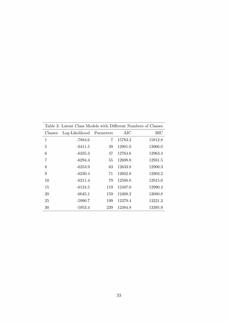
Table 3: Latent Class Models with Different Numbers of Classes

Classes Log-Likelihood Parmeters AIC BIC

1 -7884.6 7 15783.2 15812.8

5 -6411.5 39 12901.0 13066.0

6 -6335.3 47 12764.6 12963.4

7 -6294.4 55 12698.8 12931.5

8 -6253.9 63 12633.8 12900.3

9 -6230.4 71 12602.8 12903.2

10 -6211.4 79 12580.8 12915.0

15 -6124.5 119 12487.0 12990.4

20 -6045.1 159 12408.2 13080.8

25 -5990.7 199 12379.4 13221.3

30 -5953.4 239 12384.8 13395.9

33

Table 4: Latent Class Model with Eight Classes

Class: 1 2 3 4

Shares: 0.107 0.179 0.115 0.0699

Coefficients:

Fuel cost -3.546 -2.576 -1.893 -1.665

Purchase price -2.389 -5.318 -12.13 0.480

Driving radius 0.718 0.952 0.199 0.472

CMDD 0.662 1.156 0.327 1.332

PLPP 0.952 2.869 0.910 3.136

ETLS=10 dummy -1.469 -0.206 -0.113 -0.278

CV dummy -1.136 -0.553 -0.693 -2.961

Class: 5 6 7 8

Shares: 0.117 0.077 0.083 0.252

Coefficients:

Fuel cost -1.547 -0.560 -0.309 -0.889

Purchase price -2.741 -1.237 -1.397 -2.385

Driving radius 0.878 0.853 0.637 0.369

CMDD 0.514 3.400 -0.022 0.611

PLPP 0.409 3.473 0.104 1.244

ETLS=10 dummy 0.086 -0.379 -0.298 -0.265

CV dummy -3.916 -2.181 -0.007 2.656

Table 5: Standard Errrors for Latent Class Model

Class 1 Means Std devs

Est. SE Est. SE Est. SE

Share: 0.107 0.0566

Coefficients:

Fuel cost -3.546 2.473 -1.648 0.141 0.966 0.200

Purchase price -2.389 6.974 -3.698 0.487 3.388 0.568

Driving radius 0.718 0.404 0.617 0.078 0.270 0.092

CMDD 0.662 1.713 0.882 0.140 0.811 0.126

PLPP 0.952 1.701 1.575 0.240 1.098 0.178

ETLS=10 dummy -1.469 0.956 -0.338 0.102 0.411 0.089

CV dummy -1.136 3.294 -0.463 1.181 2.142 0.216

34

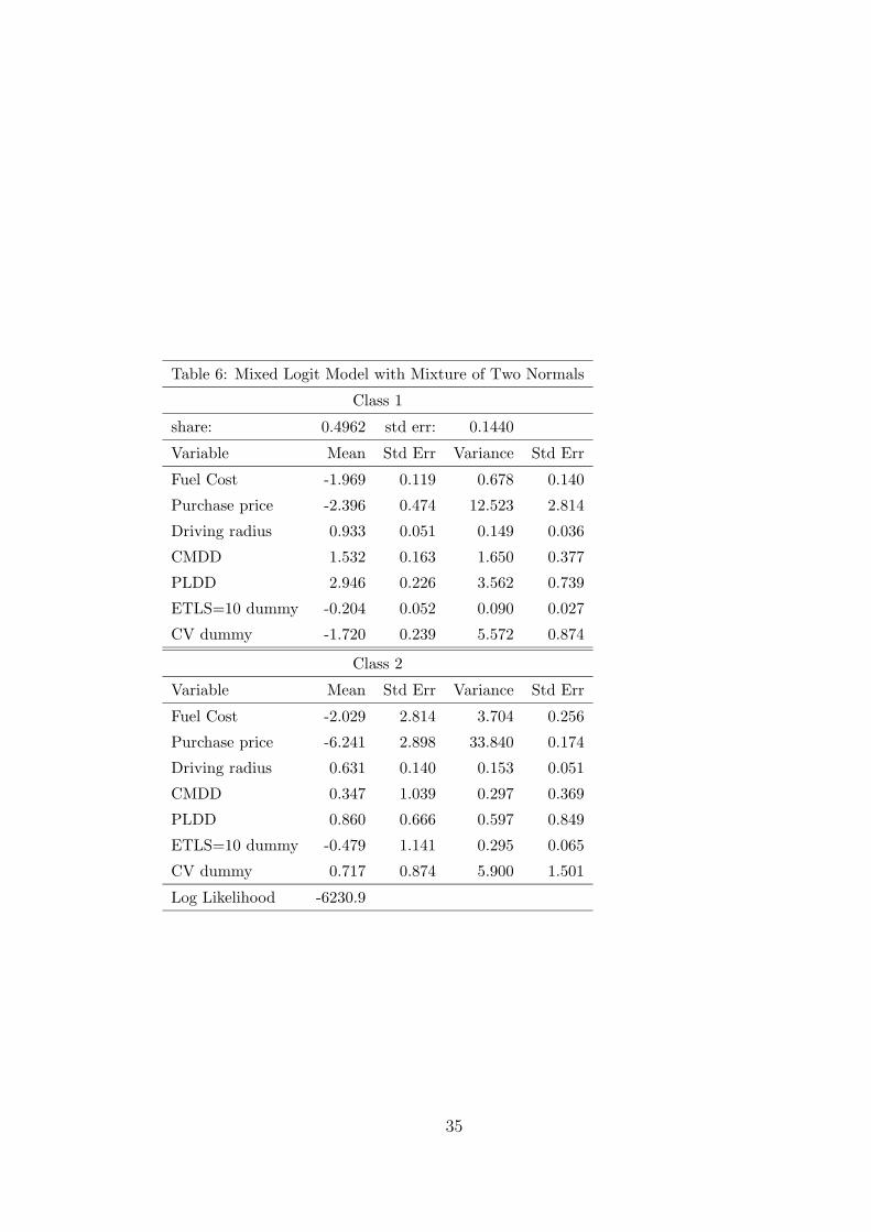
Table 6: Mixed Logit Model with Mixture of Two Normals

Class 1

share: 0.4962 std err: 0.1440

Variable Mean Std Err Variance Std Err

Fuel Cost -1.969 0.119 0.678 0.140

Purchase price -2.396 0.474 12.523 2.814

Driving radius 0.933 0.051 0.149 0.036

CMDD 1.532 0.163 1.650 0.377

PLDD 2.946 0.226 3.562 0.739

ETLS=10 dummy -0.204 0.052 0.090 0.027

CV dummy -1.720 0.239 5.572 0.874

Class 2

Variable Mean Std Err Variance Std Err

Fuel Cost -2.029 2.814 3.704 0.256

Purchase price -6.241 2.898 33.840 0.174

Driving radius 0.631 0.140 0.153 0.051

CMDD 0.347 1.039 0.297 0.369

PLDD 0.860 0.666 0.597 0.849

ETLS=10 dummy -0.479 1.141 0.295 0.065

CV dummy 0.717 0.874 5.900 1.501

Log Likelihood -6230.9

35

Table 7: Mixed Logit with Fixed Points

Halton Grid 1 Grid 2

Points: 10,000 78,125 233,280

Coefficients:

Fuel cost mean -1.869 -1.943 -1.938

stdev 1.304 1.478 1.462

Purchase price mean -4.639 -4.753 -4.762

stdev 4.586 5.163 5.125

Driving radius mean 0.591 0.638 0.634

stdev 0.306 0.438 0.434

CMDD mean 1.121 1.113 1.119

stdev 1.103 1.263 1.254

PLPP mean 1.852 1.919 1.919

stdev 1.449 1.588 1.572

ETLS=10 dummy mean -0.486 -0.476 -0.481

stdev 0.442 0.575 0.575

CV dummy mean -0.595 -0.614 -0.610

stdev 2.341 2.486 2.484

LL -6089.1 -6021.8 -6019.1

36

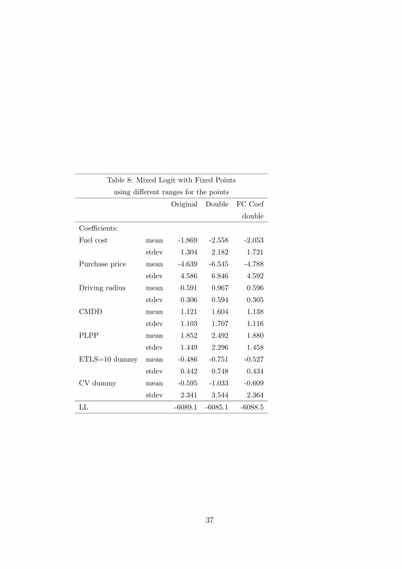
Table 8: Mixed Logit with Fixed Points

using different ranges for the points

Original Double FC Coef

double

Coefficients:

Fuel cost mean -1.869 -2.558 -2.053

stdev 1.304 2.182 1.721

Purchase price mean -4.639 -6.545 -4.788

stdev 4.586 6.846 4.592

Driving radius mean 0.591 0.967 0.596

stdev 0.306 0.594 0.305

CMDD mean 1.121 1.604 1.138

stdev 1.103 1.707 1.116

PLPP mean 1.852 2.492 1.880

stdev 1.449 2.296 1.458

ETLS=10 dummy mean -0.486 -0.751 -0.527

stdev 0.442 0.748 0.434

CV dummy mean -0.595 -1.033 -0.609

stdev 2.341 3.544 2.364

LL -6089.1 -6085.1 -6088.5

37

38

39

40

41

42

43