Ellipsoidal Geometry and Conformal Mapping KAI BORRE
58
Ellipsoidal Geometry and Conformal Mapping by KAI BORRE Preliminary version March 2001
Transcript of Ellipsoidal Geometry and Conformal Mapping KAI BORRE
Ellipsoidal Geometry
and
Conformal Mapping
by
KAI BORRE
Preliminary version March 2001
Foreword
Most geodetically oriented textbooks on ellipsoidal geometry and conformal mapping arewritten in the German language. This has motivated me to compile a useful English textfor students who follow the English M.Sc. programme in “GPS Technology” at AalborgUniversity.
The main bulk of the present text is taken from my Danish textbook “Landmåling”.However the Gauss mid-latitude formulas for solving the geodetic problems have beensubstituted by Bessel’s solution. The latter is a little more evolved but we arrive at formulasvalid for points thousands of kilometers apart.
A good textbook of differential geometry that supports and augments the presenttext is Struik (1988). I also expect some students will be happy with Guggenheimer (1977)when dealing with specialized topics.
Fjellerad, March 2001
Kai Borre
Copyright c© 2001 by Kai Borre
All rights reserved. No part of this work may be reproduced or stored or transmittedby any means, including photocopying, without the written permission of the publisher.Translation in any language is strictly prohibited—authorized translations are arranged.
Contents
Foreword ii
1 Geometry of the Ellipsoid 11.1 The Ellipsoid of Revolution 11.2 Principal Curvatures 41.3 Length of a Meridional Arc 71.4 Normal Section and the Geodesic 81.5 Frenet’s Formulas for a Geodesic 101.6 Clairaut’s Equation 131.7 The Behaviour of the Geodesic 171.8 The Direct and the Inverse Geodetic Problems 18
1.8.1 Basic differential equations fords anddσ , dλ anddω 181.8.2 The formulas for transformation ofσ to s 201.8.3 The formulas for transformation ofω to λ 221.8.4 Algorithms 24
1.9 The Ellipsoidal System Extended to Outer Space 26
2 Conformal Mappings of the Ellipsoid 292.1 Conformality 292.2 The Gaussian Mapping of the Ellipsoid onto the Plane 302.3 Transformation of Cartesian to Geographical Coordinates 332.4 Meridian Convergence and Scale 352.5 Multiplication of the Mapping 382.6 Universal Transverse Mercator 392.7 The Gaussian Conformal Mapping of the Sphere into the Plane 412.8 Arc-to-Chord Correction 452.9 Correction of Distance 472.10 Summary of Corrections 482.11 Best PossibleConformal Mapping 48
References 51
Index 53
iii

iv Contents
1Geometry of the Ellipsoid
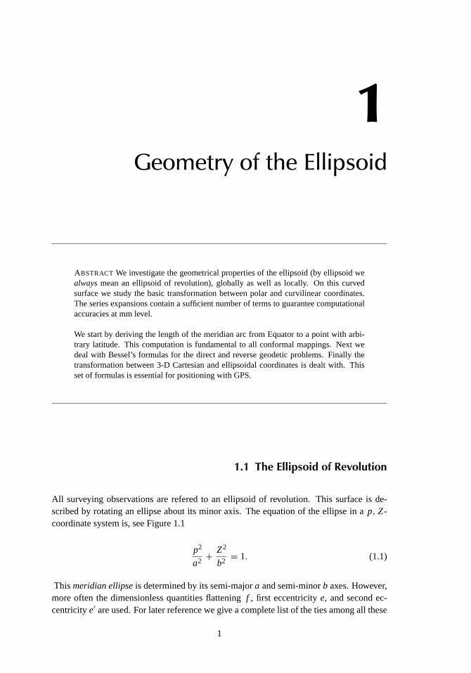
ABSTRACT We investigate the geometrical properties of the ellipsoid (by ellipsoid wealwaysmean an ellipsoid of revolution), globally as well as locally. On this curvedsurface we study the basic transformation between polar and curvilinear coordinates.The series expansions contain a sufficient number of terms to guarantee computationalaccuracies at mm level.
We start by deriving the length of the meridian arc from Equator to a point with arbi-trary latitude. This computation is fundamental to all conformal mappings. Next wedeal with Bessel’s formulas for the direct and reverse geodetic problems. Finally thetransformation between 3-D Cartesian and ellipsoidal coordinates is dealt with. Thisset of formulas is essential for positioning with GPS.
1.1 The Ellipsoid of Revolution
All surveying observations are refered to an ellipsoid of revolution. This surface is de-scribed by rotating an ellipse about its minor axis. The equation of the ellipse in ap, Z-coordinate system is, see Figure 1.1
p2
a2+ Z2
b2= 1. (1.1)
Thismeridian ellipseis determined by its semi-majora and semi-minorb axes. However,more often the dimensionless quantities flatteningf , first eccentricitye, and second ec-centricitye′ are used. For later reference we give a complete list of the ties among all these
1
2 1 Geometry of the Ellipsoid
Z
p
Equator
a
bp Q = (p, Z)
P
SouthPole
ϕ
F
G
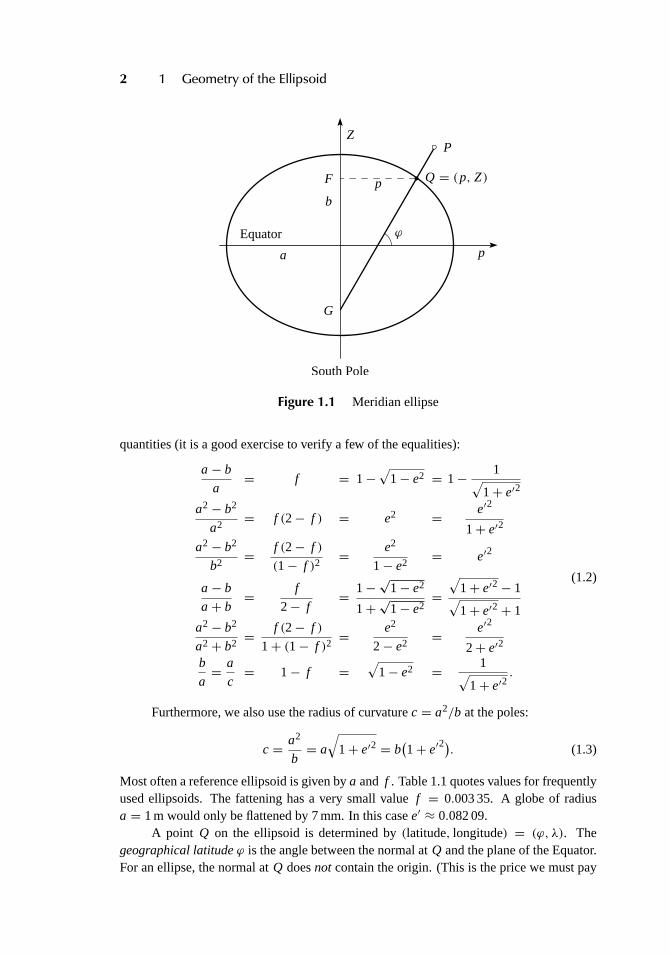
Figure 1.1 Meridian ellipse
quantities (it is a good exercise to verify a few of the equalities):
a− b
a= f = 1−
√1− e2 = 1− 1√
1+ e′2
a2− b2
a2= f (2− f ) = e2 = e′2
1+ e′2
a2− b2
b2= f (2− f )
(1− f )2= e2
1− e2= e′2
a− b
a+ b= f
2− f= 1−
√1− e2
1+√
1− e2=√
1+ e′2− 1√1+ e′2+ 1
a2− b2
a2+ b2= f (2− f )
1+ (1− f )2= e2
2− e2= e′2
2+ e′2b
a= a
c= 1− f =
√1− e2 = 1√
1+ e′2.
(1.2)
Furthermore, we also use the radius of curvaturec = a2/b at the poles:
c = a2
b= a
√1+ e′2 = b
(1+ e′2
). (1.3)
Most often a reference ellipsoid is given bya and f . Table 1.1 quotes values for frequentlyused ellipsoids. The fattening has a very small valuef = 0.003 35. A globe of radiusa = 1 m would only be flattened by 7 mm. In this casee′ ≈ 0.082 09.
A point Q on the ellipsoid is determined by(latitude, longitude) = (ϕ, λ). Thegeographical latitudeϕ is the angle between the normal atQ and the plane of the Equator.For an ellipse, the normal atQ doesnot contain the origin. (This is the price we must pay
1.1 The Ellipsoid of Revolution 3
Table 1.1 Parameters for reference ellipsoids
Name a f = (a− b)/a[m]
International 1924 6 378 388 1/297Krassovsky 1948 6 378 245 1/298.3International 1980 6 378 137 1/298.257World Geodetic System 1984 6 378 137.0 1/298.257 223 563
for flattening;ϕ is not the angle from the center of the ellipse.) Thegeographical longitudeλ is the angle between the plane of the meridian ofQ and the plane of a reference meridian(through Greenwich).
λϕ
λ = 0
Q = (ϕ, λ)
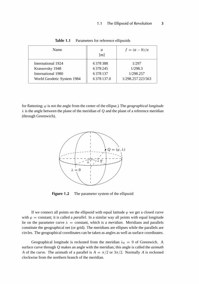
Figure 1.2 The parameter system of the ellipsoid
If we connect all points on the ellipsoid with equal latitudeϕ we get a closed curvewith ϕ = constant; it is called aparallel. In a similar way all points with equal longitudelie on the parameter curveλ = constant, which is ameridian. Meridians and parallelsconstitute the geographical net (or grid). The meridians are ellipses while the parallels arecircles. The geographical coordinates can be taken as angles as well as surface coordinates.
Geographical longitude is reckoned from the meridianλ0 = 0 of Greenwich. Asurface curve throughQ makes an angle with the meridian; this angle is called theazimuthA of the curve. The azimuth of a parallel isA = π/2 or 3π/2. Normally A is reckonedclockwise from the northern branch of the meridian.
4 1 Geometry of the Ellipsoid
1.2 Principal Curvatures
Planes that contain the surface normal atP are callednormal planes. In order to investigatethe curvature of a surface at a pointP we intersect the surface with normal planes withvarious azimuths.
Next the radius of curvatureR of the intersecting curves, normal sections, betweenthe surface and the normal planes can be determined. The two normal sections having thelargestR1 and the smallestR2 values are of special interest. Those normal sections areorthogonal.
The socalledGaussian curvatureK = (R1R2)−1 is often used to define theGaussian
osculating spherewith radiusR= √R1R2.Thecurvatureκ of a normal section making the angleα with the principal curvature
plane belonging toR1 is given byEuler’s formula
κ = cos2 α
Rmin+ sin2 α
Rmax. (1.4)
A plane that does not contain the surface normal is inclined. The radius of curvaturefor an inclined plane equals the radius of curvature in the corresponding normal sectionRtimes cosine of the angleθ between the planes. This is calledMeusnier’s theorem
ρ = Rcosθ. (1.5)
To determine the principal curvature for the normal sections of the ellipsoid we only needa few simple geometrical considerations. Any meridian plane is a plane of symmetry, sothe direction of the meridian is a direction of principal curvature. We call the radius ofcurvatureM in this direction and the radius of curvature in the orthogonal direction iscalledN. The ellipsoid is flattened at the poles and accordingly the curvature at any pointis larger in the direction of the meridian soM is smaller thanN. N is also called theprimevertical radius of curvature.
Euler’s and Meusnier’s formulas give full information concerning the curvature ofany curve throughQ on the surface.
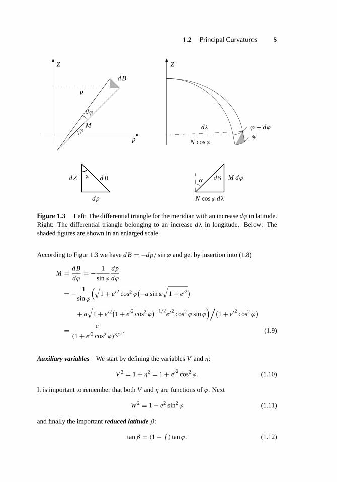
From Figure 1.3 we haved B = M dϕ or M = d B/dϕ. We want to express thelength of arcd B as a function of latitudeϕ and start from equation (1.1) for the ellipse.The relation between latitudeϕ and the Cartesian coordinates(p, Z) of a point of theellipse is given as
tanϕ = − dp
d Z. (1.6)
From (1.1) we may expressp explicitly as a function ofZ. We differentiate and insert into(1.6)
tanϕ =(a
b
)2 Z
p. (1.7)
We want to eliminateZ from (1.7) and insert from (1.1) and use (1.2) and get
p = a cosϕ√cos2 ϕ + b2
a2 sin2 ϕ
= a√
1+ e′2 cosϕ√1+ e′2 cos2 ϕ
. (1.8)
1.2 Principal Curvatures 5
p
Z
M
p
dB
ϕ
dϕ
dZ dB
dp
ϕ
ϕ + dϕϕ
dλ
Z
N cosϕ
M dϕdS
N cosϕ dλ
α
Figure 1.3 Left: The differential triangle for the meridian with an increasedϕ in latitude.Right: The differential triangle belonging to an increasedλ in longitude. Below: Theshaded figures are shown in an enlarged scale
According to Figur 1.3 we haved B= −dp/ sinϕ and get by insertion into (1.8)
M = d B
dϕ= − 1
sinϕ
dp
dϕ
= − 1
sinϕ
(√1+ e′2 cos2 ϕ
(−a sinϕ√
1+ e′2)
+ a√
1+ e′2(1+ e′2 cos2 ϕ
)−1/2e′2 cos2 ϕ sinϕ
)/(1+ e′2 cos2 ϕ
)
= c
(1+ e′2 cos2 ϕ)3/2. (1.9)
Auxiliary variables We start by defining the variablesV andη:
V2 = 1+ η2 = 1+ e′2 cos2 ϕ. (1.10)
It is important to remember that bothV andη are functions ofϕ. Next
W2 = 1− e2 sin2 ϕ (1.11)
and finally the importantreduced latitudeβ:
tanβ = (1− f ) tanϕ. (1.12)
6 1 Geometry of the Ellipsoid
This can be rewritten assinϕ = V sinβ
cosϕ = W cosβ
}. (1.13)
We collect many useful relations:
cosϕ
cosβ=
√1− e2 sin2 ϕ = 1√
1+ e′2 sin2 β
= W = V√1+ e′2
sinϕ
sinβ=√
1+ e′2 cos2 ϕ = 1√1− e2 cos2 β
= W√1− e2
= V
dϕ
dβ= W2
1− e2= V2
√1+ e′2
tanβ
tanϕ= b
a= 1− f =
√1− e2 = 1√
1+ e′2.
(1.14)
Now (1.9) can be expressed as
M = c
V3or M = a(1− e2)
(1− e2 sin2 ϕ)3/2. (1.15)
In order to calculateN we consider at pointQ both the circle of the parallel and thecircle of curvature. They lie in different planes the traces of which in Figure 1.1 are thelinesQGandQF. The line sectionQF= p is radius for the parallel andN is the radius ofcurvature in the normal section atQ; they make the angleϕ and according to the theoremof Meusnier (1.5) we get
p = N cosϕ. (1.16)
Comparing with (1.8) we get
N = a√
1+ e′2√1+ e′2 cosϕ
= c
V
and using (1.14) once again we get
N = c
V= c
√1+ e′2 sin2 β. (1.17)
Eliminatingc from (1.15) and (1.17) yields
V2 = N
M. (1.18)
TheGaussian curvatureK for the ellipsoidis
K = 1√M N= V2
c.
1.3 Length of a Meridional Arc 7
The radius of curvature at the poles areM90 = N90 = c = a2/b. The radius of curvatureat Equator isM0 = b2/a andN0 = a. The radius of curvature in a direction of azimuthαis according to (1.4)
1
RA= cos2 α
M+ sin2 α
N= 1+ η2 cos2 α
N. (1.19)
In subsequent sections we often need derivatives ofV andη2 as defined in (1.10).Once and for all we calculate their derivatives with respect toϕ:
dη2
dϕ= e′22 cosϕ(− sinϕ) = −2η2 tanϕ. (1.20)
Following geodetic tradition, we introduce
t = tanϕ (1.21)
and get
dη2
dϕ= −2η2t (1.22)
d2η2
dϕ2= −2η2(1− t2) (1.23)
d3η2
dϕ3= 8η2t. (1.24)
Similarly starting from (1.10) we get
dV
dϕ= −η
2t
V(1.25)
d2V
dϕ2= − η
2
V3
(1− t2+ η2) (1.26)
d3V
dϕ3= η2t
V5
(4+ 5η2+ 3η2t2+ η4). (1.27)
1.3 Length of a Meridional Arc
When dealing with conformal mapping equations we often need to compute the length ofthe arc of a meridian between two points with latitudesϕ1 andϕ2. From (1.15) we have
B12 =∫ ϕ2
ϕ1
M dϕ = c∫ ϕ2
ϕ1
dϕ
V3.
This integration leads to an elliptic integral of the second kind; from a computational pointof view this is no useful path to follow. Instead we develop the denominator into a series
V−3 = 1− 3
2e′2 cos2 ϕ + 15
8e′4 cos4 ϕ − 35
16e′6 cos6 ϕ +− · · ·
8 1 Geometry of the Ellipsoid
B
A
B1A1
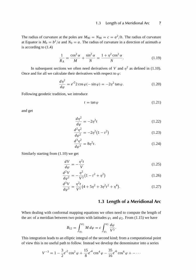
Figure 1.4 Forward and reverse normal sections
and integrate term-wise. For the international ellipsoid 1924 withc = 6 399 936.608 1 mande′2 = 0.006 768 170 the arc lengthB in meters from Equatorϕ1 = 0 to the latitudeϕ2 = ϕ, in radians, becomes
B = 6 367 654.500ϕ − 32 282.118 64 sinϕ cosϕ
× (1− 0.004 228 875 cos2 ϕ + 0.000 022 402 cos4 ϕ). (1.28)
Example 1.1 Givenϕ = 56◦, find B.
B = 6 223 646.055− 14 965.729 60(1− 0.001 322 355+ 0.000 002 190)
= 6 208 700.083 m.
1.4 Normal Section and the Geodesic
All normals to the surface of a sphere contain the center of the sphere. A normal plane atpoint A containing pointB also contains the surface normal atB. However on the ellipsoidthe surface normals atA andB only intersect ifA andB lie on the same meridian or thesame parallel. In all other cases the surface normals are skew to each other.
A normal plane at pointA containing pointB does not contain the surface normal atB and the normal plane atB containing pointA does not contain the surface normal atA.Both planes incline to each other. They cut the surface of the ellipsoid in different curves.This fact is illustrated in Figure 1.4. The pointsAA1B define the normal plane ofA andthe pointsBB1A define the normal plane atB. The forward and the reverse sight over thesame side do not coincide and we have to define which curve shall make the basis for ourcomputations.
It would be natural to choose one of thenormal sections; but the formulas becomecomplicated. In the 1700-years one often used the secantAB. But since the publicationGauss (1827) appeared one only uses thegeodesicwhich is a curve lying between theforward and the reverse normal sections, see Figure 1.5.
1.4 Normal Section and the Geodesic 9
A
B
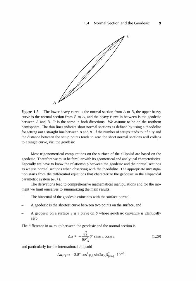
Figure 1.5 The lower heavy curve is the normal section fromA to B, the upper heavycurve is the normal section fromB to A, and the heavy curve in between is the geodesicbetweenA and B. It is the same in both directions. We assume to be on the northernhemisphere. The thin lines indicate short normal sections as defined by using a theodolitefor setting out a straight line betweenA andB. If the number of setups tends to infinity andthe distance between the setup points tends to zero the short normal sections will collapsto a single curve, viz. the geodesic
Most trigonometrical computations on the surface of the ellipoisd are based on thegeodesic. Therefore we must be familiar with its geometrical and analytical characteristics.Espcially we have to know the relationship between the geodesic and the normal sectionsas we use normal sections when observing with the theodolite. The appropriate investiga-tion starts from the differential equations that characterize the geodesic in the ellipsoidalparametric system(ϕ, λ).
The derivations lead to comprehensive mathematical manipulations and for the mo-ment we limit ourselves to summarizing the main results:
– The binormal of the geodesic coincides with the surface normal
– A geodesic is the shortest curve between two points on the surface, and
– A geodesic on a surfaceS is a curve onS whose geodesic curvature is identicallyzero.
The difference in azimuth between the geodesic and the normal section is
1α ≈ − η2A
6N2A
S2 sinαA cosαA (1.29)
and particularly for the international ellipsoid
1α[′′] ≈ −2.8′′ cos2 ϕA sin 2αAS2[km] · 10−6.
10 1 Geometry of the Ellipsoid
t
b
n
normalplane
rectifyingplane
osculatingplane
curve
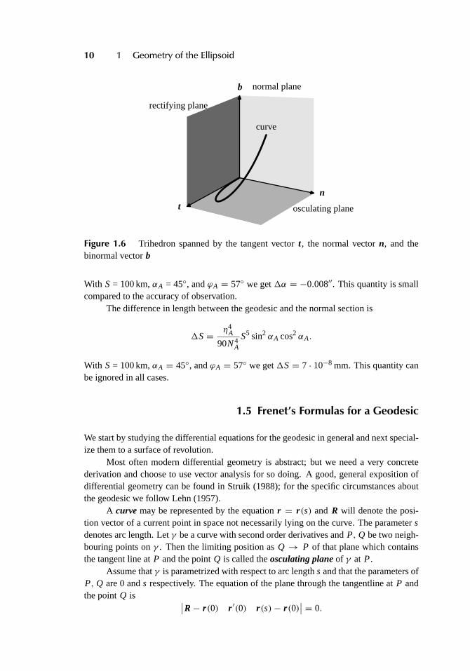
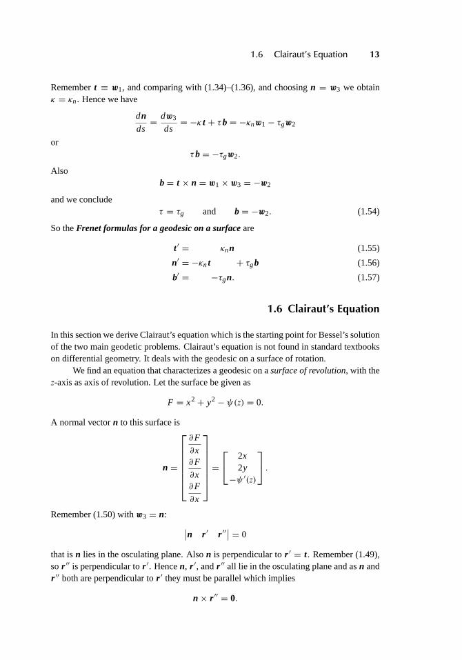
Figure 1.6 Trihedron spanned by the tangent vectort, the normal vectorn, and thebinormal vectorb
With S = 100 km,αA = 45◦, andϕA = 57◦ we get1α = −0.008′′. This quantity is smallcompared to the accuracy of observation.
The difference in length between the geodesic and the normal section is
1S= η4A
90N4A
S5 sin2 αA cos2 αA.
With S= 100 km,αA = 45◦, andϕA = 57◦ we get1S= 7 · 10−8 mm. This quantity canbe ignored in all cases.
1.5 Frenet’s Formulas for a Geodesic
We start by studying the differential equations for the geodesic in general and next special-ize them to a surface of revolution.
Most often modern differential geometry is abstract; but we need a very concretederivation and choose to use vector analysis for so doing. A good, general exposition ofdifferential geometry can be found in Struik (1988); for the specific circumstances aboutthe geodesic we follow Lehn (1957).
A curvemay be represented by the equationr = r (s) and R will denote the posi-tion vector of a current point in space not necessarily lying on the curve. The parametersdenotes arc length. Letγ be a curve with second order derivatives andP, Q be two neigh-bouring points onγ . Then the limiting position asQ → P of that plane which containsthe tangent line atP and the pointQ is called theosculating planeof γ at P.
Assume thatγ is parametrized with respect to arc lengths and that the parameters ofP, Q are 0 ands respectively. The equation of the plane through the tangentline atP andthe pointQ is ∣∣R− r (0) r ′(0) r (s)− r (0)
∣∣ = 0.
1.5 Frenet’s Formulas for a Geodesic 11
It is convenient to denote differentiation with respect to arc lengths by a prime; with thisconvention we get
r (s)− r (0) = sr ′(0)+ 12s2r ′′(0)+ o(s2)
and the equation of the osculating plane is∣∣R− r (0) r ′(0) r ′′(0)
∣∣ = 0.
The unit tangent vectort becomest = r ′. (1.30)
The vectort ′ = r ′′ (1.31)
lies in the osculating plane and is also normal tot. A unit vector along the principal normalis denoted byn and thecurvatureby κ and we have
t ′ = κn. (1.32)
Thebinormal lineat P is the normal in a direction orthogonal to the osculating plane. Thesense of the unit vectorb along the binormal is chosen so that the triadt, n, andb forms aright-handed system of axes:
b= t × n. (1.33)
The relations
t ′ = κn (1.34)
n′ = −κ t + τb (1.35)
b′ = −τn (1.36)
are known as theFrenet formulasand they underlie many investigations in the theory ofcurves and surfaces. The reader is well advised to commit them to memory.
The first and the third relations have already been obtained. The second relationfollows from differentiating the identityn = b× t to get
n′ = −τn× t + b× κn = τb− κ t.
Thecurvatureκ isκ = ∣∣r ′ × r ′′
∣∣. (1.37)
Thetorsion τ is
τ =∣∣r ′ r ′′ r ′′′
∣∣κ2
. (1.38)
Let the curver lie on a sufficiently smoothsurfacein space. The surface is given by twoindependent parametersu andv:
x = f (u, v)
y = g(u, v)
z = h(u, v).
12 1 Geometry of the Ellipsoid
A point P on the surface may then be represented by the vector equation
r = r (u, v). (1.39)
For thecurve on the surfacewe may define another moving rigt-handed triad of unitvectors. We call the unit tangent vector to the curvew1. The unit vectorw3 normal to thesurface is given as
w3 =r ′u × r ′v∣∣r ′u × r ′v
∣∣ . (1.40)
The direction ofw3 can be chosen freely. Finallyw2 is defined by the vector equation
w3 = w1× w2. (1.41)
Hence this vector lies in the tangent plane for the surface and is perpendicular to the tan-gent. Setting(tangent,normal, binormal) = (w1,w2,w3) we have
w′1 = κgw2+ κnw3 (1.42)
w′2 = −κgw1 + τgw3 (1.43)
w′3 = −κnw1−τgw2. (1.44)
The curvatureκn of the normal section is
κn = w3 · r ′′. (1.45)
The geodetic curvatureκg isκg =
∣∣w3 r ′ r ′′∣∣. (1.46)
The geodetic torsionτg isτg =
∣∣w1 w3 w′3∣∣. (1.47)
For any curve we haver ′ ≡ t ≡ w1. (1.48)
It follows that r ′ · r ′ = 1 and by differentiation
r ′ · r ′′ = 0. (1.49)
Next we specialize thecurve to be a geodesic, i.e. the curve has zero geodetic curvature
κg =∣∣w3 r ′ r ′′
∣∣ = 0. (1.50)
Then the Frenet formulas reduce to
w′1 = κnw3 (1.51)
w′2 = τgw3 (1.52)
w′3 = −κnw1−τgw2. (1.53)
1.6 Clairaut’s Equation 13
Remembert ≡ w1, and comparing with (1.34)–(1.36), and choosingn = w3 we obtainκ = κn. Hence we have
dnds= dw3
ds= −κ t + τb= −κnw1− τgw2
orτb= −τgw2.
Alsob= t × n = w1× w3 = −w2
and we concludeτ = τg and b= −w2. (1.54)
So theFrenet formulas for a geodesic on a surfaceare
t ′ = κnn (1.55)
n′ = −κn t + τgb (1.56)
b′ = −τgn. (1.57)
1.6 Clairaut’s Equation
In this section we derive Clairaut’s equation which is the starting point for Bessel’s solutionof the two main geodetic problems. Clairaut’s equation is not found in standard textbookson differential geometry. It deals with the geodesic on a surface of rotation.
We find an equation that characterizes a geodesic on asurface of revolution, with thez-axis as axis of revolution. Let the surface be given as
F = x2+ y2− ψ(z) = 0.
A normal vectorn to this surface is
n =
∂F
∂x∂F
∂x∂F
∂x
=
2x2y−ψ ′(z)
.
Remember (1.50) withw3 = n:∣∣n r ′ r ′′
∣∣ = 0
that isn lies in the osculating plane. Alson is perpendicular tor ′ = t. Remember (1.49),so r ′′ is perpendicular tor ′. Hencen, r ′, andr ′′ all lie in the osculating plane and asn andr ′′ both are perpendicular tor ′ they must be parallel which implies
n× r ′′ = 0.
14 1 Geometry of the Ellipsoid
We focus on the third component of this equation:∣∣∣∣
x yx′′ y′′
∣∣∣∣ = 0
orxy′′ − yx′′ = 0
or after integrationxy′ − yx′ = constant. (1.58)
We repeat the formulas (1.118)–(1.120):
r =
xyz
=
N cosϕ cosλN cosϕ sinλ
(1+ e′2)−1N sinϕ
. (1.59)
In the last line we have made a small rewriting using (1.2). Recall the basic equation (1.16):p = N cosϕ and we have
x = p cosλ, x′ = dp
dscosλ− p sinλ
dλ
ds(1.60)
y = p sinλ, y′ = dp
dssinλ+ p cosλ
dλ
ds. (1.61)
Insertion into (1.58) yields
p2 dλ
ds= constant. (1.62)
Our next big derivation is to determinen, t, b from r . We start by bringing some usefulformulas together. From the lower right part of Figure 1.3 and (1.18) we get
dϕ
ds= cosα
M= V2 cosα
N(1.63)
dλ
ds= sinα
N cosϕ. (1.64)
Now we insert (1.64) into (1.62) and get
N cosϕ sinα = constant (1.65)
which is Clairaut’s equation: On a surface of revolution the product of the sine of theangle of the geodesic and meridian with the distance from the axis of revolution is constant.Using geographical latitudeϕ this is
a sinα0 = N cosϕ sinα = constant (1.66)
or using reduced latitudeβ on the unit sphere
sinα0 = cosβ sinα = cosβmax= constant. (1.67)
1.6 Clairaut’s Equation 15
A
B
Cψ
a
bc
α
β
γ
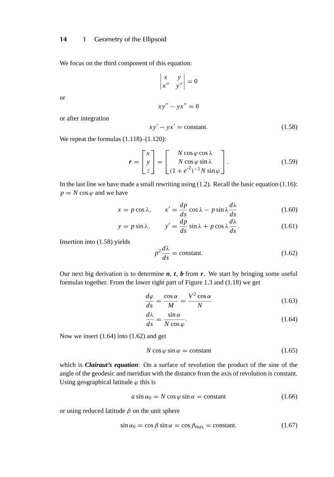
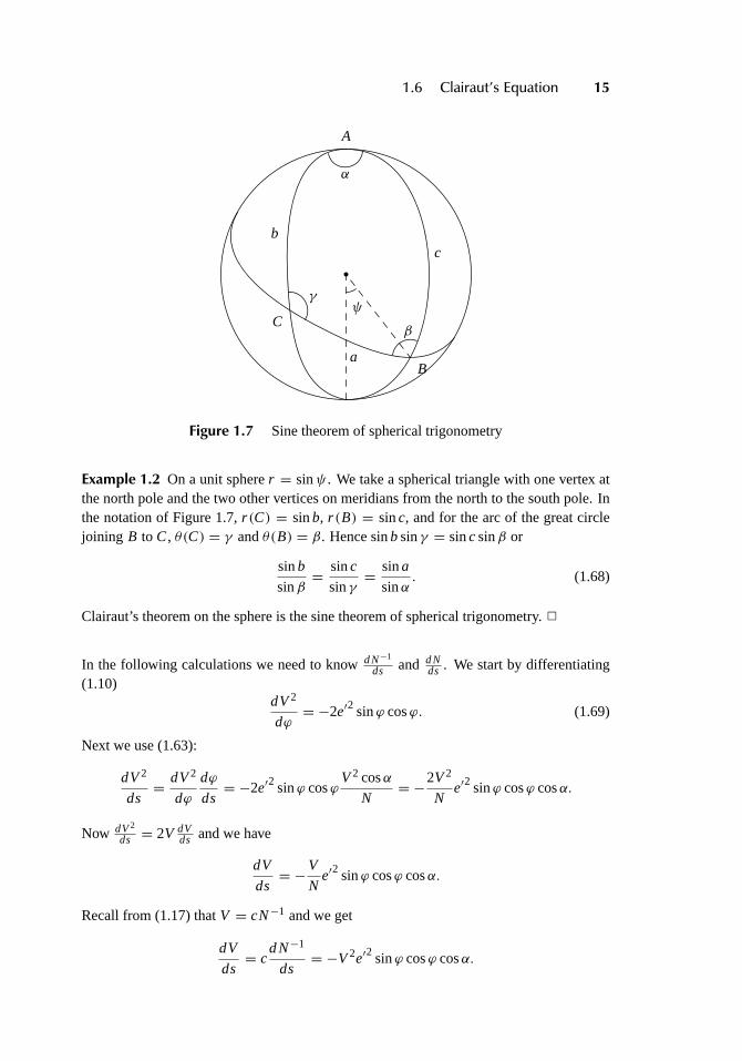
Figure 1.7 Sine theorem of spherical trigonometry
Example 1.2 On a unit spherer = sinψ . We take a spherical triangle with one vertex atthe north pole and the two other vertices on meridians from the north to the south pole. Inthe notation of Figure 1.7,r (C) = sinb, r (B) = sinc, and for the arc of the great circlejoining B to C, θ(C) = γ andθ(B) = β. Hence sinbsinγ = sincsinβ or
sinb
sinβ= sinc
sinγ= sina
sinα. (1.68)
Clairaut’s theorem on the sphere is the sine theorem of spherical trigonometry.2
In the following calculations we need to knowd N−1
ds and d Nds . We start by differentiating
(1.10)dV2
dϕ= −2e′2 sinϕ cosϕ. (1.69)
Next we use (1.63):
dV2
ds= dV2
dϕ
dϕ
ds= −2e′2 sinϕ cosϕ
V2 cosα
N= −2V2
Ne′2 sinϕ cosϕ cosα.
Now dV2
ds = 2V dVds and we have
dV
ds= −V
Ne′2 sinϕ cosϕ cosα.
Recall from (1.17) thatV = cN−1 and we get
dV
ds= c
d N−1
ds= −V2e′2 sinϕ cosϕ cosα.
16 1 Geometry of the Ellipsoid
Again d Nds = −N2 d N−1
ds and
d N
ds= e′2 sinϕ cosϕ cosα. (1.70)
In the subsequent derivations we need (1.59) and (1.63) and (1.64) and (1.70). We indicatethe calculation forx′:
x′ = dx
ds= cosϕ cosλ
d N
ds− N sinϕ cosλ
dϕ
ds− N cosϕ sinλ
dλ
ds= − cosα sinϕ cosλ− sinα sinλ.
The total result is
r ′ =
x′
y′
z′
=
− cosα sinϕ cosλ− sinα sinλ− cosα sinϕ sinλ+ sinα cosλ
cosα cosϕ
. (1.71)
Evidently
n =− cosϕ cosλ− cosϕ sinλ− sinϕ
and t = r ′ =
− cosα sinϕ cosλ− sinα sinλ− cosα sinϕ sinλ+ sinα cosλ
cosα cosϕ
and
b= t × n =− sinα sinϕ cosλ+ cosα sinλ− sinα sinϕ sinλ− cosα cosλ
sinα cosϕ
.
We return to Clairaut’s equation (1.65) and differentiate with respect to arc lengths:
d(N cosϕ sinα)
ds= d N
dscosϕ sinα − N sinϕ sinα
dϕ
ds− N cosϕ cosα
dα
ds= 0.
Inserting (1.70) and (1.63) yields
dα
ds= 1
Ntanϕ sinα. (1.72)
Using (1.63), (1.64), and (1.72) we get
n′ =
dn1
dϕ
dϕ
ds+ dn1
dλ
dλ
dsdn2
dϕ
dϕ
ds+ dn2
dλ
dλ
dsdn3
dϕ
dϕ
ds+ dn3
dλ
dλ
ds
= 1
N
V2 sinϕ cosλ cosα + sinλ sinαV2 sinϕ sinλ cosα − cosλ sinα
−V2 cosϕ cosα
.
From (1.47) we have
τg = |w1 w3 w′3| = |t n n′| = n′ · (t × n) = n′ · b
= 1
N(sinα cosα − V2 sinα cosα) = −e′ cos2 ϕ cosα sinα
N. (1.73)
1.7 The Behaviour of the Geodesic 17
βmax
−βmax
s= 0
s≈ π(1− f cosβmax)
180◦ − α0 Equator
α0
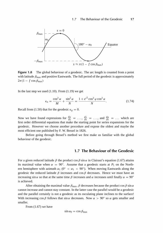
Figure 1.8 The global behaviour of a geodesic. The arc length is counted from a pointwith latitudeβmax and positive Eastwards. The full period of the geodesic is approximately2π(1− f cosβmax)
In the last step we used (1.10). From (1.19) we get
κn =cos2 α
M+ sin2 α
N= 1+ e′2 cos2 ϕ cos2 α
N. (1.74)
Recall from (1.50) that for the geodesicκg = 0.
Now we have found expressions fordϕds = . . . , dλ
ds = . . . , and dαds = . . . which are
first order differential equations that make the starting point for series expansions for thegeodesic. However we choose another procedure and expose the oldest and maybe themost efficient one published by F. W. Bessel in 1826.
Before going through Bessel’s method we first make us familiar with the globalbehaviour of the geodesic.
1.7 The Behaviour of the Geodesic
For a given reduced latitudeβ the product cosβ sinα in Clairaut’s equation (1.67) attainsits maximal value whenα = 90◦. Assume that a geodesic starts atP1 on the North-ern hemisphere with azimuthα1 (0◦ < α1 < 90◦). When moving Eastwards along thegeodesic the reduced latitudeβ increases and cosβ decreases. Hence we must have anincreasing sinα so that at the same timeβ increases andα increases until finallyα = 90◦
is achieved.After obtaining the maximal valueβmax, β decreases because the product cosβ sinα
cannot increase and cannot stay constant. In the latter case the parallel would be a geodesicand the parallel certainly is not a geodesic as its osculating plane inclines to the surface!With increasing cosβ follows that sinα decreases. Nowα > 90◦ soα gets smaller andsmaller.
From (1.67) we have
sinα0 = cosβmax
18 1 Geometry of the Ellipsoid
orα0+ βmax= 90◦. (1.75)
After crossing the Equator cosβ decreases and sinα decreases and this continues untilagainα = 90◦ andβ attains its maximal negative value. Next again sinα decreases andcosβ increases until a new crossing of Equator happens and the geodesic is on the Northernhemisphere. Forαmin andαmax we have
αmin+ αmax= 180◦. (1.76)
The geodesic continues forward with azimuths between these extremal values, that appearwhen crossing the Equator.
Any geodesic runs between a Northern and a Southern parallel of equal latitude. Thislatitude depends on the constant cosβ sinα. For a zero constant eitherα = 0◦ or β = 90◦.The first case is the meridian, the second case gives no line. If the constant is±1 we getα = 90◦ or 270◦ andβ = 0. This corresponds to the Equator.
1.8 The Direct and the Inverse Geodetic Problems
We present Bessel’s method for solving the direct and inverse geodetic problems on theellipsoid. We use Bessel’s auxiliary sphere and form differential equations similar to thoseapplied in Bessel’s original method. However, they are integrated in a different way thanthe original one. The coefficients resulting from the multiplications of the series expansionand the power functions themselves are stored and used later in the development. Thecoefficients of the expansion and the powers are all transformed to three nested coefficientsK1, K2, andK3, and two ellipsoidal corrections1σ and1ω including terms up toe8 ore′8. Therefore the accuracy of the method is higher than that of others. The following isbased on Xue-Lian (1985).
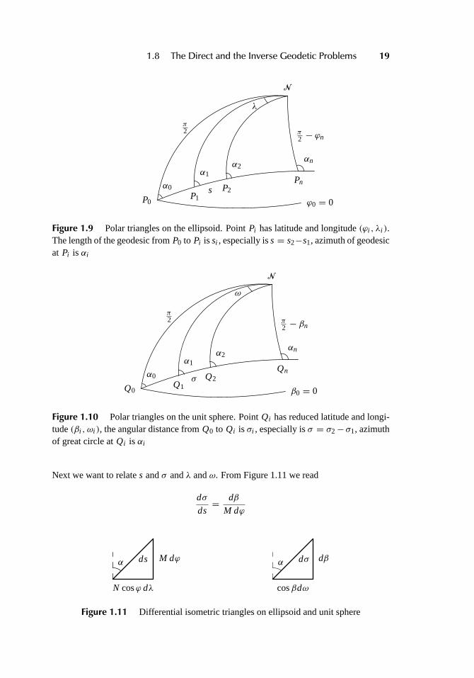
Figure 1.9 shows the geodesic elements on the ellipsoid. Figure 1.10 shows thecorresponding elements transformed on the unit auxiliary sphere one by one. The NorthPole is designated byN .
1.8.1 Basic differential equations for dsand dσ , dλ and dω
From (1.63) and (1.64) we get the differential equations of a geodesic on an ellipsoid
ds= M
cosαdϕ
dλ = M tanα
N cosϕdϕ
. (1.77)
On the unit sphere this is
dσ = 1
cosαdβ
dω = tanα
cosβdβ
. (1.78)
1.8 The Direct and the Inverse Geodetic Problems 19
N
P0P1
P2Pn
π2 π
2 − ϕn
α0
α1α2
αn
ϕ0 = 0
λ
s
Figure 1.9 Polar triangles on the ellipsoid. PointPi has latitude and longitude(ϕi , λi ).The length of the geodesic fromP0 to Pi is si , especially iss= s2−s1, azimuth of geodesicat Pi is αi
N
Q0Q1
Q2Qn
π2 π
2 − βn
α0
α1α2
αn
β0 = 0
ω
σ
Figure 1.10 Polar triangles on the unit sphere. PointQi has reduced latitude and longi-tude(βi , ωi ), the angular distance fromQ0 to Qi is σi , especially isσ = σ2− σ1, azimuthof great circle atQi is αi
Next we want to relates andσ andλ andω. From Figure 1.11 we read
dσ
ds= dβ
M dϕ
M dϕds
N cosϕ dλ
α dβdσ
cosβdω
α
Figure 1.11 Differential isometric triangles on ellipsoid and unit sphere
20 1 Geometry of the Ellipsoid
or
ds= Mdϕ
dβdσ. (1.79)
We also readM dϕ
dβ= N cosϕ dλ
dωor
dλ = M cosβ
N cosϕ
dϕ
dβdω. (1.80)
We differentiate (1.12): tanβ = (1− f ) tanϕ and remember (1.14):cosϕcosβ = W. From
(1.14) and (1.2) we get 1− f = WV and finally
dϕ
dβ= V W. (1.81)
Hence by (1.79) and (1.80), consideringM = bV W2 and from (1.18):MN = 1
V2 , we have
ds= b
Wdσ
dλ = 1
Vdω
. (1.82)
Substituting (1.14) we obtain the important equations
ds= b√
1+ e′2 sin2 β dσ (1.83)
dλ =√
1− e2 cos2 β dω. (1.84)
1.8.2 The formulas for transformation of σ to s
Using spherical trigonometric formulas for the right angled triangleQQnN in Figure 1.10,we obtain
sinβ = sinβn sinσ. (1.85)
Substituting (1.85) into (1.83), the function ofβ in (1.83) is reduced to one ofσ . We
expand√
1+ e′2 sin2 β to include the term contininge′8 and introduce the abbreviation
t = 14e′2 sin2 βn (1.86)
and get
ds= b(1+ 2t sin2 σ − 2t2 sin4 σ + 4t3 sin6 σ − 10t4 sin8 σ)dσ. (1.87)
We substitute the sine power functions ofσ in (1.87) by the cosine functions of multipleangles:
sin2 σ = 12(1− cos 2σ)
sin4 σ = 18(3− 4 cos 2σ + cos 4σ)
sin6 σ = 132(10− 15 cos 2σ + 6 cos 4σ − cos 6σ)
sin8 σ = 1128(35− 56 cos 2σ + 28 cos 4σ − 8 cos 6σ + cos 8σ)
(1.88)
1.8 The Direct and the Inverse Geodetic Problems 21
and get
ds= b((1+ t − 3
4t2+ 54t3− 175
64 t4)− t (1− t + 158 t2− 35
8 t3) cos 2σ
− 14t2(1− 3t + 35
4 t2) cos 4σ − 18t3(1− 5t) cos 6σ − 5
64t4 cos 8σ)
dσ. (1.89)
Let
K1 = 1+ t(1− 1
4t (3− t (5− 11t)))
(1.90)
K2 = t(1− t (2− 1
8t (37− 94t)))
= 1K1
t (1− t + 158 t2− 35
8 t3). (1.91)
Then
14 K 2
2 + 116t4 = 1
K1
14t2(1− 3t + 35
4 t2)
18 K 3
2 = 1K1
18t3(1− 5t).
By this (1.89) can be written as
ds= K1b(1− K2(cos 2σ + 1
4 K2(cos 4σ + 12 K2 cos 6σ))
+ 164t4(1− 4 cos 4σ − 5 cos 8σ)
)dσ. (1.92)
Now we use the integral formula∫ σ2
σ1
cosnσ dσ = 2n sin n
2(σ2− σ1) cosn2(σ2+ σ1) (1.93)
and introduce the abbreviations
s= s2− s1, σ = σ2− σ1, σm = σ2+ σ1 (1.94)
and by integrating (1.92) we have
s= K1b(σ − K2 sinσ(cosσm+ 1
4 K2(cosσ cos 2σm+ 16 K2(1+ 2 cos 2σ) cos 3σm))
+ 164t4(σ sinσ cosσ(4 cos 2σm+ 5 cos 2σ cos 4σm))
). (1.95)
Finally we introduce the abbreviations
1σ = K2 sinσ(cosσm+ 1
4 K2(cosσ cos 2σm+ 16 K2(1+ 2 cos 2σ) cos 3σm)
)(1.96)
δs= K1b 164t4(σ − sinσ cosσ(4 cos 2σm+ 5 cos 2σ cos 4σm)
)(1.97)
and gets= K1b(σ −1σ)+ δs. (1.98)
For the longests we always haveδs< 3 · 10−3 mm. So we neglectδs and solve forσ :
σ = s
K1b+1σ. (1.99)
K1 andK2 are called thenested coefficients, and1σ is called theellipsoidal reduction forthe distanceand is computed by iteration. The accuracy for the geodetic lengths will bebetter than 0.01 mm when the approximate value of1σ is sufficiently small.
22 1 Geometry of the Ellipsoid
1.8.3 The formulas for transformation of ω to λ
We expand equation (1.84) into a series containing the term ofe8:
dλ = dω − (12e2 cos2 β + 1
8e4 cos4 β + 116e6 cos6 β + 5
128e8 cos8 β)
dω. (1.100)
By (1.67)
sinα = cosβn
cosβ. (1.101)
From (1.78) we get the differential equation of a geodesic on a sphere
dω = sinα
cosβdσ.
Substituting (1.101) into above, then
dω = cosβn
cos2 βdσ. (1.102)
Substituting the above into the second term on the right side of (1.100)
dλ = dω − cosβn(1
2e2+ 18e4 cos2 β + 1
16e6 cos4 β + 5128e8 cos6 β
)dβ. (1.103)
Reducing the function ofβ to σ with (1.85)
cos2 β = 1− sin2 βn sin2 σ
cos4 β = 1− 2 sin2 βn sin2 σ + sin4 βn sin4 σ
cos6 β = 1− 3 sin2 βn sin2 σ + 3 sin4 βn sin4 σ − sin6 βn sin6 σ
. (1.104)
Hence by (1.103)
dλ = dω − cosβn((1
2e2+ 18e4+ 1
16e6+ 5128e8)− (1
8e4+ 18e6+ 15
128e8) sin2 βn sin2 σ
+ ( 116e6+ 15
128e8) sin4 βn sin4 σ − 5128e8 sin6 βn sin6 σ
)dσ. (1.105)
Using the expression off by e2
f = 12e2+ 1
8e4+ 116e6+ 5
128e8 (1.106)
as a substitute for the series ofe2 in (1.105) we have
18e4+ 1
8e6+ 5128e8 = 1
2 f 2(1+ f + f 2)
116e6+ 15
128e8 = 18 f 3(4+ 9 f )
5128e8 = 5
8 f 4.
Letv = 1
4 f sin2 βn. (1.107)
1.8 The Direct and the Inverse Geodetic Problems 23
Then (1.105) becomes
dλ=dω − f cosβn(1− 2v(1+ f + f 2) sin2 σ + 2v2(4+ 9 f ) sin4 σ − 40v3 sin6 σ
)dσ.
(1.108)Transforming the sine power functions to the cosine functions of multiple angle with (1.88)we may write
dλ = dω − f cosβn(1− v(1+ f + f 2− v(3+ 27
4 f − 252 v))
+ v(1+ f + f 2− v(4+ 9 f − 754 v)) cos 2σ + v2(1+ 9
4 f − 152 v) cos 4σ
+ 54v
3 cos 6σ)
dσ. (1.109)
Letλ = λ2− λ1, ω = ω2− ω1. (1.110)
Using (1.93) and considering (1.94) and (1.110), equation (1.109) is integrated to be theform
λ = ω − f cosβn((1− v(1+ f + f 2− v(3+ 27
4 f − 252 v)))σ
+ v(1+ f + f 2− v(4+ 9 f − 754 v)) sinσ cosσm
+ v2(1+ 94 f − 15
2 v) sinσ cosσ cos 2σ
+ 512v
3 sinσ(1+ 2 cos 2σ)) cos 3σm). (1.111)
LetK3 = v
(1+ f + f 2− v(3+ 7 f − 13v)
). (1.112)
Changing
(1− K3)− (14 f − 1
2v)v2 = 1− v(1+ f + f 2− v(3+ 27
4 f − 254 v)
)
(1− K3)K3− 14v
3 = v(1+ f + f 2− v(4+ 9 f − 754 v)
)
(1− K3)K33 − (1
4 f − 12v)v
2 = v2(1+ 94 f − 15
2 v).
Substituting into (1.111) then
λ = ω − (1− K3) f cosβn(σ + K3 sinσ(cosσm+ K3 cosσ cos 2σm)
)
− 18v
2 f 2 cosβn((1+ cos2 un)(σ − cosσ cos 2σm)
+ 16 sin2 βn(3 sinσ cosσm− 5(1+ 2 cos 2σ) cos 3σm)
). (1.113)
Let
1ω = (1− K3) f cosβn(σ + K3 sinσ(cosσm+ K3 cosσ cos 2σm)
)(1.114)
δλ = 18v
2 f 2 cosβn((1+ cos2 un)(σ − cosσ cos 2σm)
+ 16 sin2 βn(3 sinσ cosσm− 5(1+ 2 cos 2σ) cos 3σm)
). (1.115)
Thenλ = ω −1ω − δλ. (1.116)
24 1 Geometry of the Ellipsoid
The estimated maximum ofδλ for the largestλ is always less than 10−6 arcsec. Similarlyfor δSso it can be omitted. Henceλ = ω −1ω or
ω = λ+1ω. (1.117)
K3 is called a nested coefficient too, and1ω is called theellipsoid reduction for the differ-ence of longitude. It is also only found by iteration like1σ . The accuracy for the longitudedifference will be better than 10−5 arcsec when the change of the approximate value of1ω
is sufficiently small.The nested method is based on equations (1.99) and (1.117).
1.8.4 Algorithms
Direct model
1 tanβ1 = (1− f ) tanϕ1
2 tanσ1 =tanβ1
cosα1
3 cosβn = cosβ1 sinα1
4 (1) t = 14e′2 sin2 βn
(2) K1 = 1+ t(1− 1
4t (3− t (5− 11t)))
(3) K2 = t(1− t (2− 1
8t (37− 94t)))
5 (1) v = 14 f sin2 βn
(2) K3 = v(1+ f + f 2− v(3+ 7 f − 13v)
)
1σ = 0
6 (1) σ = sK1b +1σ
(2) σm = 2σ1+ σ7 1σ = K2 sinσ
(cosσm+ 1
4 K2(cosσ cos 2σm+ 16 K2(1+ 2 cos 2σ) cos 3σm)
)
Steps6 and7 are iterated until the change in1σ becomes less than a specifiedthreshold value. The initial approximation of1σ is zero.
8 (1) tanβ2 =sinβ1 cosσ + cosβ1 sinσ cosα1√
1− sin2 βn sin2(σ1+ σ)
(2) tanϕ2 =tanβ2
1− f
9 1ω = (1− K3) f cosβn(σ + K3 sinσ(cosσm+ K3 cosσ cos 2σm)
)
10 (1) tanω = sinσ sinα1
cosβ1 cosσ − sinβ1 sinσ cosα1
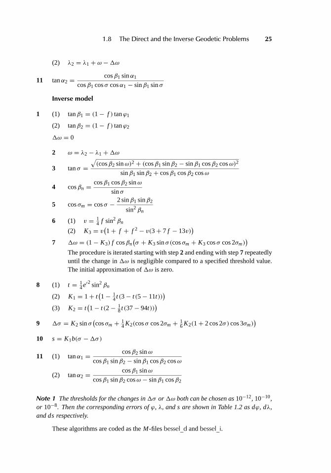
1.8 The Direct and the Inverse Geodetic Problems 25
(2) λ2 = λ1+ ω −1ω
11 tanα2 =cosβ1 sinα1
cosβ1 cosσ cosα1− sinβ1 sinσ
Inverse model
1 (1) tanβ1 = (1− f ) tanϕ1
(2) tanβ2 = (1− f ) tanϕ2
1ω = 0
2 ω = λ2− λ1+1ω
3 tanσ =√(cosβ2 sinω)2+ (cosβ1 sinβ2− sinβ1 cosβ2 cosω)2
sinβ1 sinβ2+ cosβ1 cosβ2 cosω
4 cosβn =cosβ1 cosβ2 sinω
sinσ
5 cosσm = cosσ − 2 sinβ1 sinβ2
sin2 βn
6 (1) v = 14 f sin2 βn
(2) K3 = v(1+ f + f 2− v(3+ 7 f − 13v)
)
7 1ω = (1− K3) f cosβn(σ + K3 sinσ(cosσm+ K3 cosσ cos 2σm)
)
The procedure is iterated starting with step2 and ending with step7 repeatedlyuntil the change in1ω is negligible compared to a specified threshold value.The initial approximation of1ω is zero.
8 (1) t = 14e′2 sin2 βn
(2) K1 = 1+ t(1− 1
4t (3− t (5− 11t)))
(3) K2 = t(1− t (2− 1
8t (37− 94t)))
9 1σ = K2 sinσ(cosσm+ 1
4 K2(cosσ cos 2σm+ 16 K2(1+ 2 cos 2σ) cos 3σm)
)
10 s= K1b(σ −1σ)
11 (1) tanα1 =cosβ2 sinω
cosβ1 sinβ2− sinβ1 cosβ2 cosω
(2) tanα2 =cosβ1 sinω
cosβ1 sinβ2 cosω − sinβ1 cosβ2
Note 1 The thresholds for the changes in1σ or1ω both can be chosen as10−12, 10−10,or 10−8. Then the corresponding errors ofϕ, λ, ands are shown in Table 1.2 asdϕ, dλ,andds respectively.
These algorithms are coded as theM-files bessel_d andbessel_i.
26 1 Geometry of the Ellipsoid
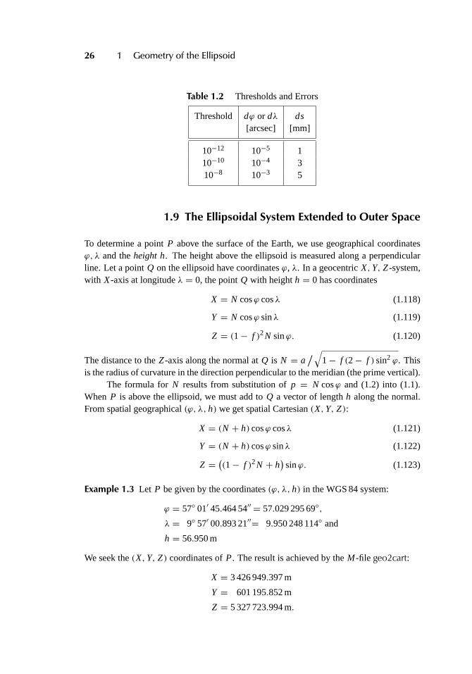
Table 1.2 Thresholds and Errors
Threshold dϕ or dλ ds[arcsec] [mm]
10−12 10−5 110−10 10−4 310−8 10−3 5
1.9 The Ellipsoidal System Extended to Outer Space
To determine a pointP above the surface of the Earth, we use geographical coordinatesϕ, λ and theheighth. The height above the ellipsoid is measured along a perpendicularline. Let a pointQ on the ellipsoid have coordinatesϕ, λ. In a geocentricX,Y, Z-system,with X-axis at longitudeλ = 0, the pointQ with heighth = 0 has coordinates
X = N cosϕ cosλ (1.118)
Y = N cosϕ sinλ (1.119)
Z = (1− f )2N sinϕ. (1.120)
The distance to theZ-axis along the normal atQ is N = a/√
1− f (2− f ) sin2 ϕ. Thisis the radius of curvature in the direction perpendicular to the meridian (the prime vertical).
The formula forN results from substitution ofp = N cosϕ and (1.2) into (1.1).When P is above the ellipsoid, we must add toQ a vector of lengthh along the normal.From spatial geographical(ϕ, λ, h) we get spatial Cartesian(X,Y, Z):
X = (N + h) cosϕ cosλ (1.121)
Y = (N + h) cosϕ sinλ (1.122)
Z = ((1− f )2N + h)
sinϕ. (1.123)
Example 1.3 Let P be given by the coordinates(ϕ, λ, h) in the WGS 84 system:
ϕ = 57◦ 01′ 45.464 54′′= 57.029 295 69◦,λ = 9◦ 57′ 00.893 21′′= 9.950 248 114◦ and
h = 56.950 m
We seek the(X,Y, Z) coordinates ofP. The result is achieved by theM-file geo2cart:
X = 3 426 949.397 m
Y = 601 195.852 m
Z = 5 327 723.994 m.
1.9 The Ellipsoidal System Extended to Outer Space 27
Z
X,Y
Q
Ph
ϕ
N
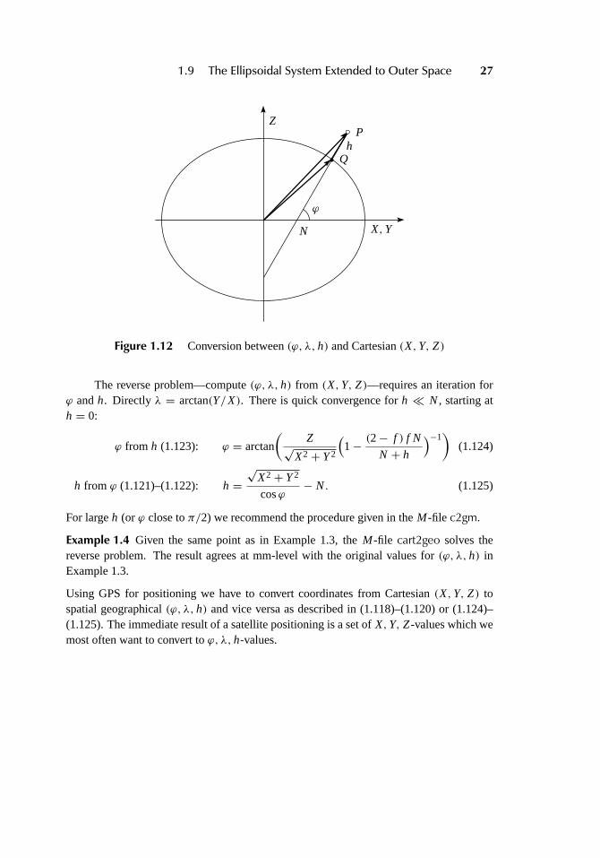
Figure 1.12 Conversion between(ϕ, λ, h) and Cartesian(X,Y, Z)
The reverse problem—compute(ϕ, λ, h) from (X,Y, Z)—requires an iteration forϕ andh. Directly λ = arctan(Y/X). There is quick convergence forh � N, starting ath = 0:
ϕ from h (1.123): ϕ = arctan
(Z√
X2+ Y2
(1− (2− f ) f N
N + h
)−1)
(1.124)
h from ϕ (1.121)–(1.122): h =√
X2+ Y2
cosϕ− N. (1.125)
For largeh (or ϕ close toπ/2) we recommend the procedure given in theM-file c2gm.
Example 1.4 Given the same point as in Example 1.3, theM-file cart2geo solves thereverse problem. The result agrees at mm-level with the original values for(ϕ, λ, h) inExample 1.3.
Using GPS for positioning we have to convert coordinates from Cartesian(X,Y, Z) tospatial geographical(ϕ, λ, h) and vice versa as described in (1.118)–(1.120) or (1.124)–(1.125). The immediate result of a satellite positioning is a set ofX,Y, Z-values which wemost often want to convert toϕ, λ, h-values.
28 1 Geometry of the Ellipsoid
2Conformal Mappings of the
Ellipsoid
ABSTRACT All mappings used in geodesy are conformal. This implies that dicrctionsonly need a second order correction while distances need a noteable correction thatcannot be neglected.
We establish the necessary theory for understanding the characteristics of the mappings.We derive the explicit formulas for the transformations(ϕ, λ)→ (x, y) and(x, y)→(ϕ, λ) as well as formulas for the meridian convergence and the scale.
These formulas are adopted for the Universal Transverse Mercator mapping (UTM).
Finally we add comments on the issue of defining the best possible mapping.
2.1 Conformality
Globally the Universal Transverse Mercator mapping (UTM) is by far the most used one.To a lesser extent conformal conical and stereographic mappings are in use.
For UTM the variation of scale is of the order of 4·10−4. Conformal mappings havesmall the corrections for directions. The image of an infinitesimal figure fits—conformsto—the original figure in the sense that they have approximately the same form. Howeverm varies from point to point, so a large figure may have an image the form of which deviatesmarkedly from the original figure. This fact is very desirable as small figures in the fieldhence become similar to the mapped ones. Any conformal mapping can be conceived as ageneralisation of a similarity transformation.
The scalem is a scalar function of position which is described by the two parameters(x, y). In casem is constant the mapping becomes a proper similarity transformation. Ifespeciallym= 1 the mapping is isometric.
UTM is based on a conformal mapping theory described by C. F. Gauss and we wantto give a detailed exposition of just this method. In doing so we follow Großmann (1976).
29
30 2 Conformal Mappings of the Ellipsoid
Equator
y
xB
B
λλ0
l
PϕPf
P
P0
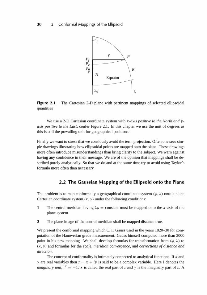
Figure 2.1 The Cartesian 2-D plane with pertinent mappings of selected ellipsoidalquantities
We use a 2-D Cartesian coordinate system withx-axis positive to the North andy-axis positive to the East, confer Figure 2.1. In this chapter we use the unit of degrees asthis is still the prevailing unit for geographical positions.
Finally we want to stress that we consiously avoid the term projection. Often one sees sim-ple drawings illustrating how ellipsoidal points are mapped onto the plane. These drawingsmore often introduce misunderstandings than bring clarity to the subject. We warn againsthaving any confidence in their message. We are of the opinion that mappings shall be de-scribed purely analytically. So that we do and at the same time try to avoid using Taylor’sformula more often than necessary.
2.2 The Gaussian Mapping of the Ellipsoid onto the Plane
The problem is to map conformally a geographical coordinate system(ϕ, λ) onto a planeCartesian coordinate system(x, y) under the following conditions:
1 The central meridian havingλ0 = constant must be mapped onto thex-axis of theplane system.
2 The plane image of the central meridian shall be mapped distance true.
We present the conformal mapping which C. F. Gauss used in the years 1820–30 for com-putation of the Hanoverian grade measurement. Gauss himself computed more than 3000point in his new mapping. We shall develop formulas for transformation from(ϕ, λ) to(x, y) and formulas for thescale, meridian convergence, andcorrections of distance anddirection.
The concept of conformality is intimately connected to analytical functions. Ifx andy are real variables thenz = x + iy is said to be a complex variable. Herei denotes theimaginary unit, i 2 = −1. x is called the real part ofz andy is the imaginary part ofz. A
2.2 The Gaussian Mapping of the Ellipsoid onto the Plane 31
function f (z) is called analytical at a pointz = z0 if f is defined and has a derivative atany point in a neighbourhood ofz0. The function is called analytical in a regionD if it isanalytical at any point inD. Polynomials with complex constantsc0, . . . , cn of the form
f (z) = c0+ c1z+ c2z2+ · · · + cnzn (2.1)
are analytical in the whole plane.The length differentialdScan be expressed in geographical coordinates(ϕ, λ):
dS2 = M2 dϕ2+ (N cosϕ)2 dλ2.
We want to use complex function theory. This is only possible ifdϕ anddλ have a factorin common. To obtain this, we introduce the following substitution:
dq = M
N cosϕdϕ. (2.2)
The new variableq is called isometric latitude. Let e denote the eccentricity, then theexplicit expression forq is
q =∫ ϕ
0
M
N cosξdξ = ln
(tan(π4 + ϕ
2
)(1− esinϕ
1+ esinϕ
)e/2). (2.3)
Substitutingdq we getdS2 = N2 cos2 ϕ(dq2+ dλ2).
Now let l be the difference in longitude between the meridian containing the arbitrary pointP and the central meridianλ0. We describe a conformal mapping through the analyticalfunction F :
x + iy = F(q + i l ). (2.4)
The origin at the ellipsoid of revolution is taken as the intersection between the centralmeridian and Equator. This gives the first boundary condition (l = 0 for y = 0), condition1 above:
xy=0 = F(q).
The second boundary condition tells that the meridian arc from Equator to the point withisometric latitudeq (corresponding to the geographical latitudeϕ) equalsB, condition2above:
xy=0 = B = F(q). (2.5)
Consequently the analytical functionF measuress the meridional arc as a function of iso-metric latitude. We are not interested inF itself, but rather its derivatives:
dx = d B= Mdϕ = N cosϕ dq.
The last equality follows from (2.2). We divide byq:
dx
dq= d B
dq= d F(q)
dq= F ′(q) = N cosϕ.
32 2 Conformal Mappings of the Ellipsoid
According to the assumptionsl = λ − λ0 is small (a few degrees), butϕ andq can takeon any value between 0◦ og 90◦. In order to work with small values both forl andq weintroduce an auxillary pointP0 on the central meridian. (In case of DenmarkP0 often hasthe value of 56◦ north latitude.) In all further computations we work withdifferences ingeographic and isometric latitude:
ϕ − ϕ0 = 1ϕ, q − q0 = 1q.
We insert these differences into (2.4)
x + iy = F(q0+1q + i l ).
Next we expandF into a Taylor series around the pointP0:
x + iy = F(q)0+ F ′(q)0(1q + i l )+ 1
2F ′′(q)0(1q + i l )2
+ 1
6F ′′′(q)0(1q + i l )3+ · · · . (2.6)
Remember from (2.5) thatF(q)0 = B so
x + iy = B+(
d B
dq
)
0(1q + i l )+ 1
2
(d2B
dq2
)
0(1q + i l )2
+ 1
6
(d3B
dq3
)
0(1q + i l )3+ · · · . (2.7)
Let the coefficients in the series bea1, a2, . . . and we putx − B = 1x. Then the approxi-mated mapping equation is
1x + iy = a1(1q + i l )+ a2(1q + i l )2+ a3(1q + i l )3+ · · · (2.8)
with
a1 =(
d B
dq
)
0=(
d B
dϕ
dϕ
dq
)
0=(
MN cosϕ
M
)
0= N0 cosϕ0
a2 =1
2
(d2B
dq2
)
0= 1
2
(d
dϕ
d B
dq
dϕ
dq
)
0= −1
2N0 cos2 ϕ0 t0
a3 =1
6
(d3B
dq3
)
0= 1
6
(d
dϕ
d2B
dq2
dϕ
dq
)
0= −1
6N0 cos3 ϕ0(1− t2
0 + η20)
a4 =1
24
(d4B
dq4
)
0= 1
24
(d
dϕ
d3B
dq3
dϕ
dq
)
0= 1
24N0 cos4 ϕ0 t0(5− t2
0
+ 9η20 + 4η4
0)
a5 =1
120
(d5B
dq5
)
0= 1
120
(d
dϕ
d4B
dq4
dϕ
dq
)
0= 1
120N0 cos5 ϕ0(5− 18t2
0
+ t40 + · · · )
. (2.9)
2.3 Transformation of Cartesian to Geographical Coordinates 33
Separating the real and the imaginary parts in (2.8) we obtain the series for1x and1y.On the right side we have powers of1q andl .
Still looking for simple formulas we introduce a trick: In stead of using the auxiliarypoint P0 on the central meridian as expansion point we introduce another point of expan-sion, namelyPϕ which also is on the central meridian and having the same latitudeϕ asthe point to be mapped. Then follows that1ϕ = 1q = 0 and in the parenteses in (2.8) isonly left i l . Separation into the real and the imaginary parts yields
x = B− a2l 2+ a4l 4+ · · ·y = a1l − a3l 3+ a5l 5− · · ·
, (2.10)
The coefficientsai shall be computed for latitudeϕ. The final mapping equations read
x = B+ 1
2N cos2 ϕ tl 2+ 1
24N cos4 ϕ t (5− t2+ 9η2)l 4+ · · ·
y = N cosϕ l + 1
6N cos3 ϕ(1− t2+ η2)l 3
+ 1
120N cos5 ϕ(5− 18t2+ t4)l 5+ · · ·
. (2.11)
2.3 Transformation of Cartesian to Geographical Coordinates
The transformation consists of two steps. First we compute the isometric ellipsoidal co-ordinates from the Cartesian coordinates. Next the isometric latitude is converted to geo-graphical latitude. We change from Cartesian to isometric coordinates by using the inversefunction f of F :
q + i l = f (x + iy). (2.12)
The boundary conditions forF are
q l=0 = f (x) = f (B) and f ′(x) = dq
d B= 1
N cosϕ.
The right side of (2.12) can again be developed at the pointP0 and withq − q0 = 1q andx − B0 = 1x, we get
1q + i l =(
dq
d B
)
0(1x + iy)+ 1
2
(d2q
d B2
)
0(1x + iy)2
+ 1
6
(d3q
d B3
)
0(1x + iy)3+ · · · (2.13)
or introducing a set of coefficientsbi :
1q + i l = b1(1x + iy)+ b2(1x + iy)2+ b3(1x + iy)3
+ b4(1x + iy)4+ b5(1x + iy)5+ · · · . (2.14)
34 2 Conformal Mappings of the Ellipsoid
Explicitly the coefficientsbi are
b1 =(
dq
d B
)
0= 1
N0 cosϕ0
b2 =1
2
(d2q
d B2
)
0= t0
2N20 cosϕ0
b3 =1
6
(d3q
d B3
)
0= 1+ 2t2
0 + η20
6N30 cosϕ0
b4 =1
24
(d4q
d B4
)
0= t0(5+ 6t2
0 + η20 − 4η4
0)
24N40 cosϕ0
b5 =1
120
(d5q
d B5
)
0= 5+ 28t2
0 + 24t40 + · · ·
120N50 cosϕ0
. (2.15)
Again the series expansion takes place at the footpointPf = (ϕ f , 0) of P0. So1x = 0and the separation into the real and the imaginary parts yields
1q = −b2y2+ b4y4− · · ·l = b1y− b3y3+ b5y5− · · ·
. (2.16)
The coefficientsbi must be computed forϕ f .We do not seek1q but rather1ϕ. The transition from1q to1ϕ also happens by
means of a series in which we introduce1ϕ = ϕ − ϕ f and1q = q − qf
ϕ − ϕ f = d11q + d2(1q)2+ · · ·
with
d1 =(
dϕ
dq
)
f= cosϕ f (1+ η2
f ); d2 =1
2
(d2ϕ
dq2
)
f= −1
2cos2 ϕ f t f (1+ 4η2
f ).
Insertion of1q yields
ϕ − ϕ f = −b2d1y2+ (b4d1+ b22d2)y
4+ · · · .
Finally, by inserting the coefficientsbi anddi we get
ϕ = ϕ f −t f
2N2f
(1+ η2f )y
2+ t f
24N4f
(5+ 3t2f + 6η2
f − 6η2f t2
f )y4+ · · ·
l = 1
Nf cosϕ fy−
1+ 2t2f + η2
f
6N3f cosϕ f
y3+5+ 28t2
f + 24t4f
120N5f cosϕ f
y5+ · · ·
. (2.17)
For |l | < 3◦ these series guarantee an accuracy at the mm-level when the latitudeϕ is nottoo large because thent increases rapidly.
2.4 Meridian Convergence and Scale 35
Pϕ
Pf
q = const.
x = const.
P
l = const.y = const.
γ
γ
dy
dx m√
E dqm√
E dl
x
Figure 2.2 Meridian convergence
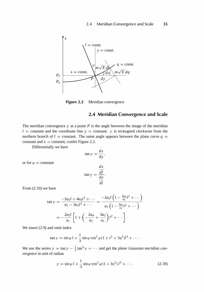
2.4 Meridian Convergence and Scale
The meridian convergenceγ at a pointP is the angle between the image of the meridianl = constant and the coordinate liney = constant.γ is reckogned clockwise from thenorthern branch ofl = constant. The same angle appears between the plane curveq =constant andx = constant, confer Figure 2.2.
Differentially we have
tanγ = dx
dy,
or for ϕ = constant
tanγ =dx
dldy
dl
.
From (2.10) we have
tanγ = −2a2l + 4a4l 3+ · · ·a1− 3a3l 2+ · · · =
−2a2l(1− 2a4
a2l 2+ · · ·
)
a1
(1− 3a3
a1l 2+ · · ·
)
= −2a2l
a1
[1+
(−2a4
a2+ 3a3
a1
)l 2+ · · ·
].
We insert (2.9) and omit index
tanγ = sinϕ l + 1
3sinϕ cos2 ϕ(1+ t2+ 3η2)l 3+ · · · .
We use the seriesγ = tanγ − 13 tan3 γ + · · · and get theplane Gaussian meridian con-
vergencein unit of radian
γ = sinϕ l + 1
3sinϕ cos2 ϕ(1+ 3η2) l 3+ · · · . (2.18)
36 2 Conformal Mappings of the Ellipsoid
From Figure 2.2 we also get forx = constant:
tanγ = m√
E dq
m√
E dl=
∂q
∂y∂l∂y
An expansion similar to above yields
tanγ = −2b2y+ 4b4y3+ · · ·b1− 3b3y3+ · · · =
2b2y
b1
[1+
(−2b4
b2+ 3b3
b1
)y2+ · · ·
]
eller med koefficienterne fra (2.15) og tanγ = γ + · · ·
γ = t f
Nfy− t f
3N3f
(1+ t2f − η2
f )y3+ · · · .
For conformal mapping there exists a close relationship between scalem and meridianconvergenceγ . However, this connection only can be demonstrated to its full extent andbeauty by using analytical functions. Here we limit ourselves to quote the following result:
msinγ = − ∂y
∂B; mcosγ = ∂x
∂B.
These equations can be checked by insertion into (2.19) below.
Scalem as function ofϕ and l Thescalem is defined at the ratio between the elementaryarc element on the ellipsoiddSand its plane imageds in the Cartesian coordinate system:
m2 = ds2
dS2= E
E
dx2+ dy2
dq2+ dl2= 1
N2 cos2 ϕ
[(∂x
∂q
)2
+(∂y
∂q
)2]
= 1
N2 cos2 ϕ
[(∂x
∂B
)2
+(∂y
∂B
)2](
d B
dq
)2
.
Remember thatd B/dq = N cosϕ and consequently
m2 =(∂x
∂B
)2
+(∂y
∂B
)2
. (2.19)
From (2.9) and (2.10) we get
∂x
∂B= 1− da2
dq
dq
d Bl 2+ da4
dq
dq
d Bl 4+ · · ·
∂y
∂B= da1
dq
dq
d Bl − da3
dq
dq
d Bl 3+ · · · ,
da1
dq= 2a2,
da2
dq= 3a3,
da3
dq= 4a4,
da4
dq= 5a5,
dq
d B= a−1
1 ,
2.4 Meridian Convergence and Scale 37
∂x
∂B= 1+ 1
2cos2 ϕ(1− t2+ η2)l 2+ 1
24cos4 ϕ(5− 18t2+ t4)l 4+ · · ·
∂y
∂B= − cosϕ t l − 1
6cos3 ϕ t (5− t2+ · · · )l 3+ · · · .
Insertion into (2.19) gives
m2 = 1+ cos2 ϕ(1+ η2)l 2+ 1
3cos4 ϕ(2− t2+ · · · )l 4+ · · ·
or taking the square root
m= 1+ 1
2cos2 ϕ(1+ η2)l 2+ 1
24cos4 ϕ(5− 4t2+ · · · )l 4+ · · · .
Scalem as function of y A similar expression form as function ofy can be detrmnedthrough the following derivation. We start from the inverse expression of (2.19):
1
m2=(∂B
∂x
)2
+(∂B
∂y
)2
.
So we have to calculate the partial derivatives ofB with respect tox andy. Therefore wemust find expressions forB that are functions of those variables. This can be achieved byexpandingf (B) = f
(x + (B− x)
)into a Taylor series:
f (B) = f (x)+ f ′(x)(B− x)+ 12 f ′′(x)(B− x)2+ · · · . (2.20)
By insertion of
f (B) = q, f (x) = qf , f ′(x) =(
dq
d B
)
f, etc.
and (2.15), equation (2.20) becomes:
q − qf = 1q = b1(B− x)+ b2(B− x)2+ · · · .
But from (2.16) we also have
1q = −b2y2+ b4y4+ · · · .
Equating the two expressions and solving for(B− x) we get
B− x = −b2
b1y2+ b4
b1y4− b2
b1(B− x)2+ · · · .
We approximate(B− x) by the first term on the right side:
B = x − b2
b1y2+
(b4
b1− b3
2
b31
)y4+ · · · .
38 2 Conformal Mappings of the Ellipsoid
From (2.15) we insertbi
B = x − t f
2Nfy2+ t f
24N3f
(5+ 3t2f + · · · )y4+ · · · . (2.21)
Now we differentiate at the pointPf
∂B
∂x= − t f
Nfy+ 1
6N3f
(5t f + 3t3f + · · · )y3+ · · · .
When we want to derive with respect tox we explicitly have to go via geographical latitudeϕ:
∂B
∂x= ∂B
∂ϕ
∂ϕ
∂x= ∂B
∂ϕ
∂ϕ
∂B= ∂B
∂ϕ
V2
N.
We differentiate (2.21) with respect tox and use
dt
dϕ= 1+ t2,
d N−1
dϕ= − η2t
N V2
∂B
∂x= 1− 1
2N2f
(1+ t2f + η2
f )y2+ 1
24N4f
(5+ 14t2f + 9t4
f + · · · )y4+ · · · .
Insertion into (2.4) yields
1
m2= 1−
1+ η2f
N2f
y2+ 2
3N4f
y4+ · · ·
or finally from the binomial formula
m= 1+1+ η2
f
2N2f
y2+ 1
24N4f
y4+ · · · .
As (1+ η2)/N = 1/M this expression becomes inspherical approximation
m= 1+ 1
2R2y2+ 1
24R4y4+ · · · .
2.5 Multiplication of the Mapping
On page 30 under2 we asked that the central meridian should be mapped one-to-one(distance true). This condition can generalize so that a distance at the central meridian ismapped into a distance on thex-axis so that the two distances make a constant proportionm0 6= 1. By this (2.5) changes to
F(q) = m0B. (2.22)
Repeating earlier derivations we find thatx and y in (2.11) and (2.17) likewise shall bemultiplied bym0. If we designate coordinates defined by (2.22) withx and y we have
x = m0x and y = m0y.
2.6 Universal Transverse Mercator 39
Choosing an appropriate value form0 we can keep the scale within certain limits. Bychoosingm0 < 1 we may suppress a too large value for the scale at distances far from thecentral meridian. A guideline may be to fixm0 to a value at the central meridian that isexactly as much less than unity as the scale becomes larger than unity at the boundary ofthe mapping area. However, a reasonable “round value” is to be preferred.
2.6 Universal Transverse Mercator
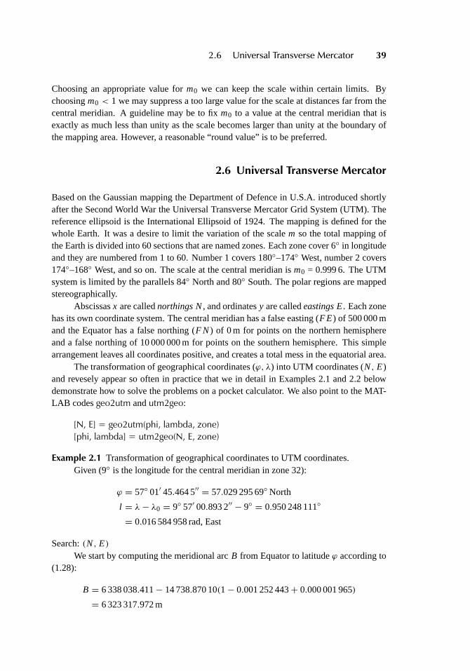
Based on the Gaussian mapping the Department of Defence in U.S.A. introduced shortlyafter the Second World War the Universal Transverse Mercator Grid System (UTM). Thereference ellipsoid is the International Ellipsoid of 1924. The mapping is defined for thewhole Earth. It was a desire to limit the variation of the scalem so the total mapping ofthe Earth is divided into 60 sections that are named zones. Each zone cover 6◦ in longitudeand they are numbered from 1 to 60. Number 1 covers 180◦–174◦ West, number 2 covers174◦–168◦ West, and so on. The scale at the central meridian ism0 = 0.999 6. The UTMsystem is limited by the parallels 84◦ North and 80◦ South. The polar regions are mappedstereographically.
Abscissasx are callednorthingsN, and ordinatesy are calledeastingsE. Each zonehas its own coordinate system. The central meridian has a false easting (F E) of 500 000 mand the Equator has a false northing (F N) of 0 m for points on the northern hemisphereand a false northing of 10 000 000 m for points on the southern hemisphere. This simplearrangement leaves all coordinates positive, and creates a total mess in the equatorial area.
The transformation of geographical coordinates (ϕ, λ) into UTM coordinates (N, E)and revesely appear so often in practice that we in detail in Examples 2.1 and 2.2 belowdemonstrate how to solve the problems on a pocket calculator. We also point to the MAT-LAB codesgeo2utm andutm2geo:
[N, E] = geo2utm(phi, lambda, zone)[phi, lambda] = utm2geo(N, E, zone)
Example 2.1 Transformation of geographical coordinates to UTM coordinates.Given (9◦ is the longitude for the central meridian in zone 32):
ϕ = 57◦ 01′ 45.464 5′′ = 57.029 295 69◦North
l = λ− λ0 = 9◦ 57′ 00.893 2′′ − 9◦ = 0.950 248 111◦
= 0.016 584 958 rad, East
Search:(N, E)We start by computing the meridional arcB from Equator to latitudeϕ according to
(1.28):
B = 6 338 038.411− 14 738.870 10(1− 0.001 252 443+ 0.000 001 965)
= 6 323 317.972 m
40 2 Conformal Mappings of the Ellipsoid
The further computations run according to (2.11):
t = 1.541 590 030
η2 = e′2 cos2 ϕ = 0.006 768 170 cos2 ϕ = 0.002 004 493
N = c
V= c√
1+ η2= 6 393 531.919 m
x = B+ N
2cos2 ϕ tl 2+ N
24cos4 ϕ t (5− t2+ 9η2)l 4
= 6 323 317.972+ 401.459+ 0.007= 6 323 719.439 m
y = N cosϕ
[1+ 1
6cos2 ϕ(1− t2+ η2)l 2
+ 1
120cos4 ϕ(5− 18t2+ t4)l 4
]l
= 57 706.116 48(1− 0.000 018 662− 0.000 000 002)
= 57 705.039 m.
Finally we get in zone 32
N = FN+m0x = 0+ 0.999 6· 6 323 719.439= 6 321 189.95 m
E = FE+m0y = 500 000+ 0.999 6· 57 705.039= 557 681.96 m
Example 2.2 Transformation of UTM coordinates to geographical coordinates.
Given: (N,E) = (6 321 189.95, 557 681.96) in zone 32.
Search:(ϕ, λ)
The first step is to compute the latitudeϕ f for the footpoint, see Figure 1.1. Thecomputation occurs iteratively according to (1.28). The first approximation is
ϕ(1)f =
Nm0
0.994 955 869c.
With the approximate valueϕ(1)f we computeB(1) from (1.28) and the next approximationis
ϕ(2)f =
Nm0− B(1)
0.994 955 869c.
The procedure is as follows
ϕ(i+1)f = ϕ(i )f +
Nm0− B(i )
0.994 955 869c
and the result
ϕ f = ϕ(n)f , whenN
m0− B(n) = 0.
2.7 The Gaussian Conformal Mapping of the Sphere into the Plane 41
Note that anyB(i ) must be computed directly from (1.28). The computation now runs asfollows
ϕ(1)f =
6 323 719.438
6 367 654.496= 0.993 100 276
B(1) = 6 308 969.718 m
ϕ(2)f = 0.993 100 276+ 6 323 719.438− 6 308 969.718
6 367 654.496= 0.995 416 627
B(2) = 6 323 749.608 m
ϕ(3)f = 0.995 416 627+ 6 323 719.438− 6 323 749.608
6 367 654.496= 0.995 411 889
B(4) = 6 323 719.378 m
ϕ(4)f = 0.995 411 889+ 6 323 719.438− 6 323 719.378
6 367 654.496= 0.995 411 898
B(4) = 6 323 719.438 m
So N/m0 − B(4) ≈ 0 and henceϕ f = 0.995 411 898 rad. The subsequent computationsare
t f = 1.541 802 493, η2f = 0.002 004 104
Nf =c√
1+ η2f
= 6 393 533.165 m
y = E − FE
m0= 557 681.96− 500 000
0.999 6= 57 705.040 m
We insert into (2.17) and get
ϕ = 0.995 411 898− 0.000 062 924+ 0.000 000 005
= 0.995 348 979 rad
l = 0.016 586 254(1− 0.000 078 152+ 0.000 000 011)
= 0.016 584 958 rad
λ = 9◦ + l .
Finally
ϕ = 57◦ 01′ 45.464 4′′
λ = 9◦ 57′ 00.893 1′′
which result is in agreement with the starting values in Example 2.1—except for the influ-ence of rounding errors.
2.7 The Gaussian Conformal Mapping of the Sphere into the Plane
In practical surveying we must know how measured directions and distances shall be cor-rected when mapped conformally from the ellipsoid into the plane. As mentioned earlier
42 2 Conformal Mappings of the Ellipsoid
π2 − A1
π2 − Y1
R
X2−X1R π
2 − Y2RS
R
P2
P1
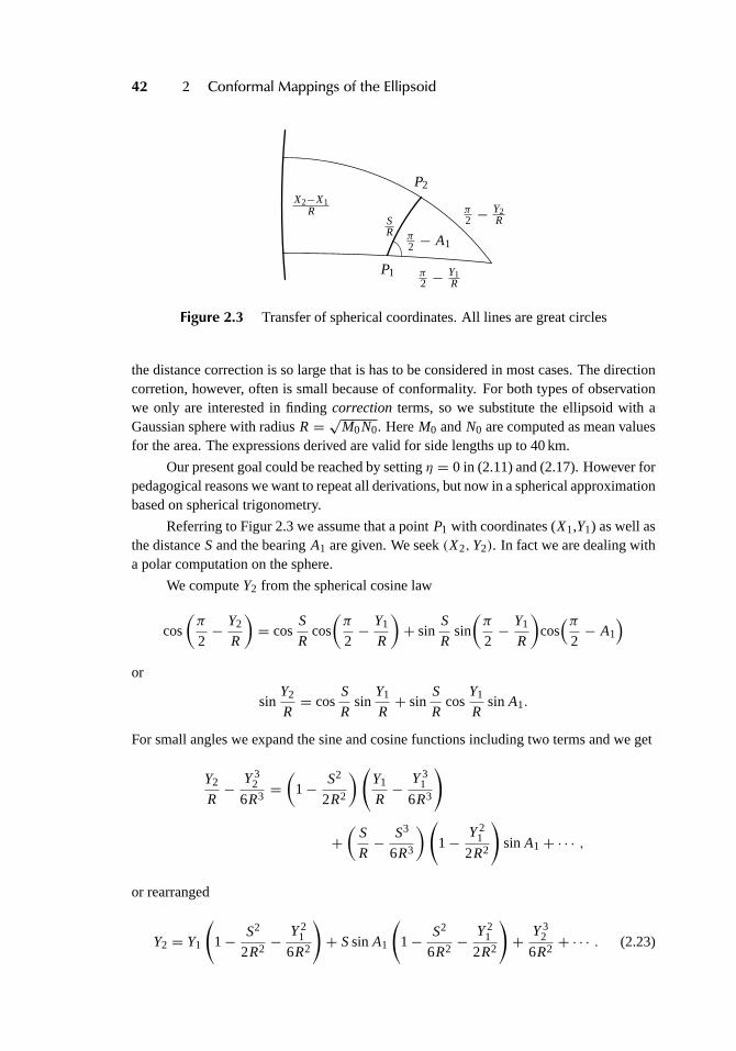
Figure 2.3 Transfer of spherical coordinates. All lines are great circles
the distance correction is so large that is has to be considered in most cases. The directioncorretion, however, often is small because of conformality. For both types of observationwe only are interested in findingcorrection terms, so we substitute the ellipsoid with aGaussian sphere with radiusR= √M0N0. HereM0 andN0 are computed as mean valuesfor the area. The expressions derived are valid for side lengths up to 40 km.
Our present goal could be reached by settingη = 0 in (2.11) and (2.17). However forpedagogical reasons we want to repeat all derivations, but now in a spherical approximationbased on spherical trigonometry.
Referring to Figur 2.3 we assume that a pointP1 with coordinates (X1,Y1) as well asthe distanceSand the bearingA1 are given. We seek(X2,Y2). In fact we are dealing witha polar computation on the sphere.
We computeY2 from the spherical cosine law
cos
(π
2− Y2
R
)= cos
S
Rcos
(π
2− Y1
R
)+ sin
S
Rsin
(π
2− Y1
R
)cos(π
2− A1
)
or
sinY2
R= cos
S
Rsin
Y1
R+ sin
S
Rcos
Y1
Rsin A1.
For small angles we expand the sine and cosine functions including two terms and we get
Y2
R− Y3
2
6R3=(
1− S2
2R2
)(Y1
R− Y3
1
6R3
)
+(
S
R− S3
6R3
)(1− Y2
1
2R2
)sin A1+ · · · ,
or rearranged
Y2 = Y1
(1− S2
2R2− Y2
1
6R2
)+ Ssin A1
(1− S2
6R2− Y2
1
2R2
)+ Y3
2
6R2+ · · · . (2.23)
2.7 The Gaussian Conformal Mapping of the Sphere into the Plane 43
The last right side term is rewritten in the following manner
Y32
6R2=(Y1+ Ssin A1
)36R2
= Y31
6R2+ Y2
1 Ssin A1
2R2+ Y1S2 sin2 A1
2R2+ S3 sin3 A1
6R2+ · · ·
and is inserted into (2.23)
Y2 = Y1+ Ssin A1−Y1S2 cos2 A1
2R2− S3 sin A1 cos2 A1
6R2− · · · .
With the new variables
ScosA1 = 1X and Ssin A1 = 1Y, (2.24)
the ordinate formula becomes
Y2 = Y1+ Ssin A1−Y1(1X)2
2R2− (1X)21Y
6R2− · · · . (2.25)
Forcomputation ofX2 we use the spherical sine law
sinX2− X1
R= sin
S
R
sin(π2 − A1
)
sin(π2 − Y2
) = sin SR
cosY2R
cosA1.
All small angles are substituted by their series expansions
X2− X1
R− (X2− X1)
3
6R3=(
S
R− S3
6R3
)(1+ Y2
2
2R2
)cosA1+ · · · (2.26)
X2− X1 = ScosA1
(1− S2
6R2+ Y2
2
2R2
)+ (X2− X1)
3
6R2+ · · · . (2.27)
We get(X2 − X1)3/6R2 = S3 cos3 A1/6R2 + · · · . By this the formula for the transfer of
the abscissa is
X2 = X1+ ScosA1+Y2
2 ScosA1
2R2− S3 sin2 A1 cosA1
6R2+ · · ·
or by using (2.24)
X2 = X1+ ScosA1+Y2
21X
2R2− 1X(1Y)2
6R2+ · · · . (2.28)
If you want to work with explicit formulasY2 can be substituted byY1+1Y+· · · . The for-mulas (2.25) and (2.28) forY2 andX2 are analogue to the plane formulas for computationof a traverse; now two correction terms are added; they vanish in the plane case(R= ∞).
By this we have derived explicit series for the computation of the coordinates for anew point based on the coordinates of a given point and a direction leaving from this givenpoint and with a known distance. In geodesy this setup also is namedthe direct problem.
44 2 Conformal Mappings of the Ellipsoid
dX dX′
Y
dY
Y = const.
X = const.
dSAdx dx
y
dy
Y = const.
X = const.
t ds
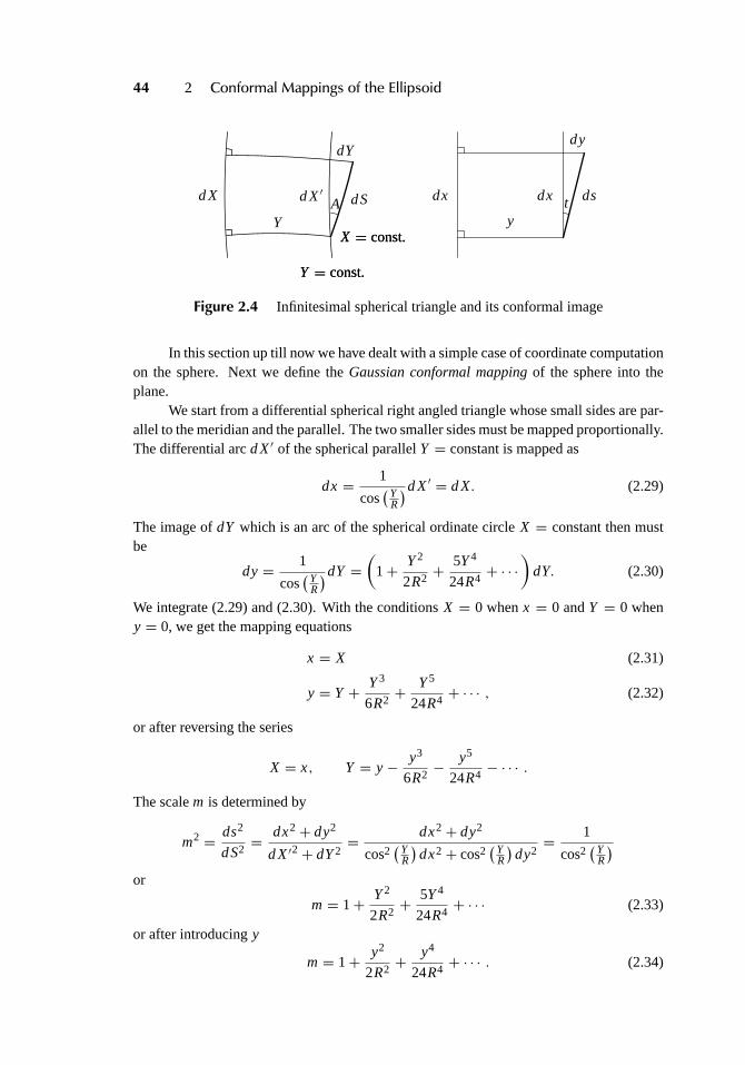
Figure 2.4 Infinitesimal spherical triangle and its conformal image
In this section up till now we have dealt with a simple case of coordinate computationon the sphere. Next we define theGaussian conformal mappingof the sphere into theplane.
We start from a differential spherical right angled triangle whose small sides are par-allel to the meridian and the parallel. The two smaller sides must be mapped proportionally.The differential arcd X′ of the spherical parallelY = constant is mapped as
dx = 1
cos(Y
R
)d X′ = d X. (2.29)
The image ofdY which is an arc of the spherical ordinate circleX = constant then mustbe
dy= 1
cos(Y
R
)dY =(
1+ Y2
2R2+ 5Y4
24R4+ · · ·
)dY. (2.30)
We integrate (2.29) and (2.30). With the conditionsX = 0 whenx = 0 andY = 0 wheny = 0, we get the mapping equations
x = X (2.31)
y = Y + Y3
6R2+ Y5
24R4+ · · · , (2.32)
or after reversing the series
X = x, Y = y− y3
6R2− y5
24R4− · · · .
The scalem is determined by
m2 = ds2
dS2= dx2+ dy2
d X′2+ dY2= dx2+ dy2
cos2(Y
R
)dx2+ cos2
(YR
)dy2= 1
cos2(Y
R
)
or
m= 1+ Y2
2R2+ 5Y4
24R4+ · · · (2.33)
or after introducingy
m= 1+ y2
2R2+ y4
24R4+ · · · . (2.34)
2.8 Arc-to-Chord Correction 45
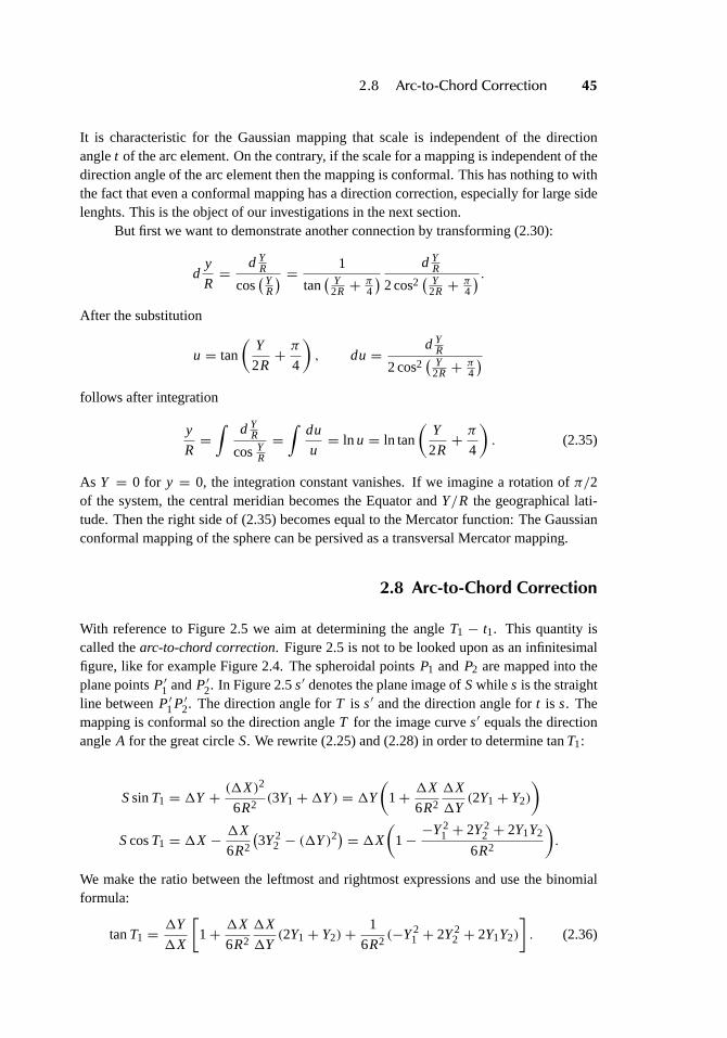
It is characteristic for the Gaussian mapping that scale is independent of the directionanglet of the arc element. On the contrary, if the scale for a mapping is independent of thedirection angle of the arc element then the mapping is conformal. This has nothing to withthe fact that even a conformal mapping has a direction correction, especially for large sidelenghts. This is the object of our investigations in the next section.
But first we want to demonstrate another connection by transforming (2.30):
dy
R= d Y
R
cos(Y
R
) = 1
tan( Y
2R + π4
) d YR
2 cos2( Y
2R + π4
) .
After the substitution
u = tan
(Y
2R+ π
4
), du= d Y
R
2 cos2( Y
2R + π4
)
follows after integration
y
R=∫
d YR
cosYR
=∫
du
u= ln u = ln tan
(Y
2R+ π
4
). (2.35)
As Y = 0 for y = 0, the integration constant vanishes. If we imagine a rotation ofπ/2of the system, the central meridian becomes the Equator andY/R the geographical lati-tude. Then the right side of (2.35) becomes equal to the Mercator function: The Gaussianconformal mapping of the sphere can be persived as a transversal Mercator mapping.
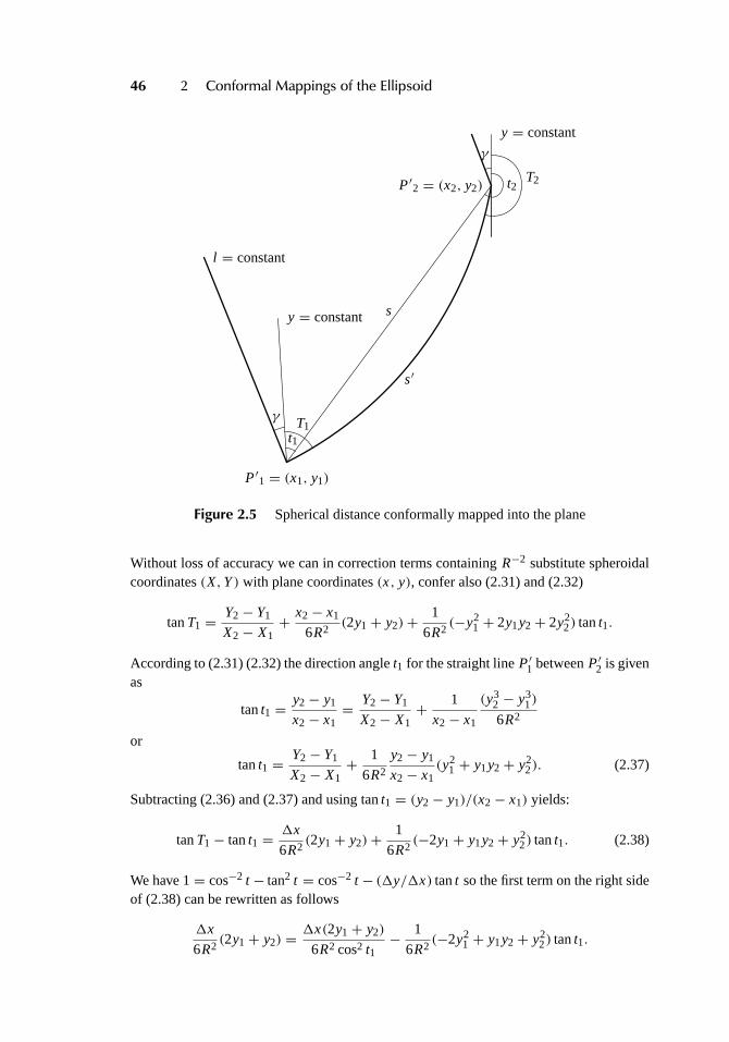
2.8 Arc-to-Chord Correction
With reference to Figure 2.5 we aim at determining the angleT1 − t1. This quantity iscalled thearc-to-chord correction. Figure 2.5 is not to be looked upon as an infinitesimalfigure, like for example Figure 2.4. The spheroidal pointsP1 and P2 are mapped into theplane pointsP′1 andP′2. In Figure 2.5s′ denotes the plane image ofSwhile s is the straightline betweenP′1P′2. The direction angle forT is s′ and the direction angle fort is s. Themapping is conformal so the direction angleT for the image curves′ equals the directionangleA for the great circleS. We rewrite (2.25) and (2.28) in order to determine tanT1:
SsinT1 = 1Y + (1X)2
6R2(3Y1+1Y) = 1Y
(1+ 1X
6R2
1X
1Y(2Y1+ Y2)
)
ScosT1 = 1X − 1X
6R2
(3Y2
2 − (1Y)2) = 1X
(1− −Y2
1 + 2Y22 + 2Y1Y2
6R2
).
We make the ratio between the leftmost and rightmost expressions and use the binomialformula:
tanT1 =1Y
1X
[1+ 1X
6R2
1X
1Y(2Y1+ Y2)+
1
6R2(−Y2
1 + 2Y22 + 2Y1Y2)
]. (2.36)
46 2 Conformal Mappings of the Ellipsoid
P′1 = (x1, y1)
l = constant
y = constant s
s′
y = constant
P′2 = (x2, y2)
γ
t1T1
γ
t2T2
Figure 2.5 Spherical distance conformally mapped into the plane
Without loss of accuracy we can in correction terms containingR−2 substitute spheroidalcoordinates(X,Y) with plane coordinates(x, y), confer also (2.31) and (2.32)
tanT1 =Y2− Y1
X2− X1+ x2− x1
6R2(2y1+ y2)+
1
6R2(−y2
1 + 2y1y2+ 2y22) tant1.
According to (2.31) (2.32) the direction anglet1 for the straight lineP′1 betweenP′2 is givenas
tant1 =y2− y1
x2− x1= Y2− Y1
X2− X1+ 1
x2− x1
(y32 − y3
1)
6R2
or
tant1 =Y2− Y1
X2− X1+ 1
6R2
y2− y1
x2− x1(y2
1 + y1y2+ y22). (2.37)
Subtracting (2.36) and (2.37) and using tant1 = (y2− y1)/(x2− x1) yields:
tanT1− tant1 =1x
6R2(2y1+ y2)+
1
6R2(−2y1+ y1y2+ y2
2) tant1. (2.38)
We have 1= cos−2 t − tan2 t = cos−2 t − (1y/1x) tant so the first term on the right sideof (2.38) can be rewritten as follows
1x
6R2(2y1+ y2) =
1x(2y1+ y2)
6R2 cos2 t1− 1
6R2(−2y2
1 + y1y2+ y22) tant1.
2.9 Correction of Distance 47
We insert this into (2.38) and the last terms vanish and we get
tanT1− tant1 =1x(2y1+ y2)
6R2 cos2 t1.
A Taylor expansion yields
tant1 = tan(T1+ (t1− T1)
) = tanT1+t1− T1
cos2 T1+ sinT1
cos3 T1(t1− T1)
2+ · · ·
or
tanT1− tant1 =T1− t1cos2 T1
.
By this thearc-to-chord correctionat the spheroidal pointP1 for the Gaussian mapping ofthe sphere into the plane
T1− t1 =(x2− x1)(2y1+ y2)
6R2. (2.39)
We emphasize that in formula (2.39)(x2−x1) denotes a difference of coordinates in north-south direction andy is the ordinate in east-west direction relative to the central meridian,confer Figure 2.5.
Example 2.3 Let x2 − x1 = 10 km, y1 = 95 km, y2 = 105 km theny13
= 98.3 km andwe obtainT1 − t1 = 0.77 mgon. The direction correction atP2 is given asT2 − t2 =(x1− x2)y1
3/2R2 with y1
3= 101.6 km. The numerical result is−0.79 mgon.
2.9 Correction of Distance
The correction of distance is easy to determine by integration of the expression for thescale. By using the binomial formula for (2.34) the result becomes
dS=(
1− y2
2R2
)ds+ · · · .
Ignoring fourth order terms we can setds= dy/ sint and get by integration
S= s−∫ y2
y1
y2
2R2
dy
sint= s− y3
2 − y31
6R2 sint= s− 1
6R2
y2− y1
sint
y32 − y3
1
y2− y1
= s− s
6R2(y2
1 + y1y2+ y22).
Accordingly thecorrection of distancefor the Gaussian mapping of the sphere onto theplane for the distance between pointsP1 andP2 is
σ = S− s= − s
6R2(y2
1 + y1y2+ y22). (2.40)
48 2 Conformal Mappings of the Ellipsoid
2.10 Summary of Corrections
We study the mapped meridian and the mapped geodesic through the pointPi . The mappedazimuthαm between the tangent to the mapped meridian and the tangent to the mappedgeodesic is identical to the ellipsoidal azimuthαe since the mapping is conformal.
The grid azimuthT of the mapped geodesic is the angle between grid northxm andthe tangent to the mapped geodesic. The grid azimuth of the chordt is the angle betweengrid north and the chordPi Pj .
To keep computations simple we utilize chords and quantites related to them as fol-lows:
– An ellipsoidal azimuth is reduced to the grid azimuth by first subtracting the meridianconvergence
Ti j = αe,i j − γi .
The grid azimuth is further reduced by the arc-to-chord correction to give the gridazimuth of the chord
ti j = Ti j − (T − t)i j .
– An ellipsodal directionde is reduced to the plane directiondm by the same direction
dm,i j = de,i j − (T − t)i j .
– An ellipsoidal angleae,i jk between dirctionsi j andik is reduced by
am,i jk = ae,i jk + (T − t)i j − (T − t)ik .
– A length of the geodesic on the ellipsoidse is transformed to the length of the mappedgeodesic by the line scalek∗ and we get
l i j = sm,i j = k∗se,i j
where the line scalek∗ is the average point scale over the line.
The expressions forγ , T − t , andk vary from one conformal mapping to another.The reader is referred to Lee (1976).
2.11 Best Possible Conformal Mapping
If one were to design a new mapping with a given purpose one might ask if certain valuesfor the scale are to be preferred to others. We then must stress that it is no quality in itselfthat the scale deviates less possible from unity. And we already have seen an examplewhere we simply change the scale by multiplying by a constant, see Section 2.5.
The basic problem was investigated by Milnor (1969). He wanted to find the bestpossible conformal mapping of a given area that must be simply connected and have a
2.11 Best Possible Conformal Mapping 49
twice differentiable boundary. “Best possible” is to be understood in the sense that the ratiommax/mmin is minimum. The problem has one solution that is derived form a boundarycurve having constant scale. This result is due to Chebyshev and has been known for morethan hundred years.
Throughout this chapter our starting point always has been how the mapping fromthe ellipsoid to the plane is defined. The description has been given in form of the explicitmapping functionF or as necessary geometrical descriptions of the mapping. From thiswe have derived—someone will maybe call it tediously—expressions for the mapping ofcoordinates, meridian convergence, scale, etc.
However, based on a lemma by Milnor we could have started in the following way:“We considertheconformal mapping whosescaleis given as . . . .”
M ILNOR’ S LEMMA : The saclem for a conformal mappingF of the elliposoid determineF up to a rotation and two translations in the plane. A positive functionm given onthe ellipsoid is connected by a conformal mapping functionF if and only if m is twicedifferentiable and satisfy the differential equation
m21 ln m= Gaussian curvature of the ellipsoid= 1
M N.
In 2-D the Laplace operator1 is1 = ∂2
∂x2 + ∂2
∂y2 . To demonstrate a use of the lemma bychecking if the UTM mapping really is conformal
m= c0+ c2y2+ c4y4+ · · · .
In casem only depends ony then1 shall be interpreted as1 = d2
dy2 . As m varies sym-metrically around the central meridian the power series only can contain even powers. Weget
d ln m
dy= 1
m
dm
dy
andd2 ln m
dy2=(
md2m
dy2−(
dm
dy
)2)/
m2
or according to Milnor
m2 d2 ln m
dy2= m
d2m
dy2−(
dm
dy
)2
= 1
M N.
We have
dm
dy= y
R2+ 4y3
24R4+ · · ·
d2m
dy2= 1
R+ 12y2
23R4+ · · ·
50 2 Conformal Mappings of the Ellipsoid
and inserting up to and including the fourth power we get
1
M N= (c0+ c2y2+ c4y4)(2c2+ 12c4y2)− (2c2y+ 4c4y3)2
= 2c0c2+ (12c0c4− 2c22)y
2− 2c2c4y4+ · · · .
For y = 0 we getc2 = 1/2c0M N. The coefficient toy2 must be zero as the expression forM N is independent ofy; hencec4 = c2
2/6c0.
m= c0+1
2c0M Ny2+ 1
24c30M2N2
y4+ · · · , (2.41)
which in spherical approximation is identical to (2.34) forc0 = 1.
Mapping freaks may find much pleasure in reading König & Weise (1951).
References
Bodemüller, H. (1954). Die geodätischen Linien des Rotationsellipsoides und die Lösungder geodätischen Hauptaufgaben für große Strecken unter besonderer Berücksichtigungder Bessel-Helmertschen Lösungsmethode, volume 13 ofDeutsche Geodätische Kommis-sion, Reihe B. Deutsches Geodätisches Forschungsinstitut, Abteilung I, München.
Gauss, Carl Frierich (1827). Disquisitiones generales circa superficies curvas. A. Wan-gerin, Leipzig.
Großmann, Walter (1976). Geodätische Rechnungen und Abbildungen in der Landesver-messung. Konrad Wittwer, Stuttgart, 3rd edition.
Guggenheimer, Heinrich W. (1977). Differential Geometry. Dover Publications, NewYork.
König, R. & Weise, K. (1951). Mathematische Grundlagen der höheren Geodäsie undKartographie. Springer, Berlin Göttingen Heidelberg.
Lee, L. P. (1976). Conformal Projections Based on Elliptic Functions, volume 16 ofCar-tographica Monograph. B. V. Gutsell, Toronto, Canada.
Lehn, C. J. (1957). The Main Problem of Geodesy and the Inverse Problem Solved by Vec-tor Methods, volume XXVI of Geodætisk Instituts Skrifter, 3. række. Geodætisk Institut,København.
Milnor, John (1969). A problem in cartography.The American Mathematical Monthly,76:1101–1112.
Struik, Dirk J. (1988). Lectures on Classical Differential Geometry. Dover Publications,New York, second edition.
Willmore, T. J. (1959). An Introduction to Differential Geometry. Clarendon Press, Ox-ford.
Xue-Lian, Zhan (1985). The nested coefficient method for accurate solutions of direct andreverse geodetic problems with any length. In7th International Symposium on GeodeticComputations, Cracow, June 18–21, pages 747–763, Institute of Geodesy and Cartogra-phy. Warsow, Poland, ul. Jasna 2/4.
51
52 References
Index
arc element, 45elementary, 31, 36
arc-to-chord correction, 45, 47arc-tochord correction, 45azimuth, 3
boundary condition, 33
central meridian, 30, 38, 45, 47, 49Chebyshev, P. L., 49conversion of coordinates
ellipsoidal and 3-D, 27coordinate system
Cartesian, 30coordinates
geographical computed from Carte-sian, 34
isometric, 33spherical, 42
correctionof direction, 41of distance, 41
correction of distance, 47cosine law
spherical, 42curvature, 4
Gaussian, 6, 49
easting, 39ellipsoid
international 1924, 9ellipsoidal coordinates
3-D, 26Euler’s formula, 4
footpoint, 34function
analytical, 30, 36
Gauss,C. F., 30Gaussian curvature, 4Gaussian sphere, 4, 42geodesic, 8–10geodesic curvature, 9great circle, 42
imaginary unit, 30
Laplace operator, 49latitude
footpoint, 40isometric, 31
latitude differenceisometric, 32
mappingconformal, 30, 41, 45, 49distance true, 30Gaussian, 29, 44, 47multiplication of, 38stereographic, 39
mapping equation, 44Mercator function, 45Mercator mapping
transversal, 45meridian, 3
central, 31meridian arc
length of, 7meridian convergence, 35, 36
plane Gaussian, 35meridian ellipse, 4Meusnier’s theorem, 4, 6Milnor, J., 48
53
54 Index
normal plane, 4, 8normal section, 4, 6, 8, 10northing, 39
parallel, 3polar computation on the sphere, 42polynomial
complex, 31
radius of curvature at Equator, 7radius of curvature at poles, 7
scale, 36, 39, 44scale as function of length, 38sine law
spherical, 43spherical trigonometry, 42surface normal, 8
transformation of geographical to UTMcoordinates, 39
transformation of UTM to geographicalcoordinates, 40, 41
traversespherical, 43
trianglespherical, 44
UTM, 29, 39zone, 39
variablecomplex, 30