Elimination Structures in Scienti c Computingpothen/Papers/ds.pdf · 2005-01-11 · Elimination...

1Elimination Structures in Scientific

Computing

Alex PothenOld Dominion University

Sivan ToledoTel-Aviv University

1.1 The elimination tree . . . . . . . . . . . . . . . . . . . . . . . . . . . . . . . . . . 1-2The elimination game • The elimination tree datastructure • An algorithm • A skeleton graph •

Supernodes

1.2 Applications of etrees . . . . . . . . . . . . . . . . . . . . . . . . . . . . . . . . . 1-8Efficient symbolic factorization • Predicting row andcolumn nonzero counts • Three classes of factorizationalgorithms • Scheduling parallel factorizations •

Scheduling out-of-core factorizations

1.3 The clique tree . . . . . . . . . . . . . . . . . . . . . . . . . . . . . . . . . . . . . . . . . 1-12Chordal graphs and clique trees • Design of efficientalgorithms with clique trees • Compact clique trees

1.4 Clique covers and quotient graphs . . . . . . . . . . . . . . . . . . 1-17Clique covers • Quotient graphs • The problem ofdegree updates • Covering the column-intersectiongraph and biclique covers

1.5 Column elimination trees and elimination DAGS 1-20The column elimination tree • Elimination DAGS •

Elimination structures for the unsymmetricmultifrontal algorithm

The most fundamental computation in numerical linear algebra is the factorization of amatrix as a product of two or more matrices with simpler structure. An important exampleis Gaussian elimination, in which a matrix is written as a product of a lower triangularmatrix and an upper triangular matrix. The factorization is accomplished by elementaryoperations in which two or more rows (columns) are combined together to transform thematrix to the desired form. In Gaussian elimination, the desired form is an upper triangularmatrix, in which nonzero elements below the diagonal have been transformed to be equalto zero. We say that the subdiagonal elements have been eliminated. (The transformationsthat accomplish the elimination yield a lower triangular matrix.)

The input matrix is usually sparse, i.e., only a few of the matrix elements are nonzeroto begin with; in this situation, row operations constructed to eliminate nonzero elementsin some locations might create new nonzero elements, called fill, in other locations, as aside-effect. Data structures that predict fill from graph models of the numerical algorithm,and algorithms that attempt to minimize fill, are key ingredients of efficient sparse matrixalgorithms.

This chapter surveys these data structures, known as elimination structures, and the al-gorithms that construct and use them. We begin with the elimination tree, a data structure

0-8493-8597-0/01/$0.00+$1.50

c© 2001 by CRC Press, LLC 1-1

1-2

associated with symmetric Gaussian elimination, and we then describe its most importantapplications. Next we describe other data structures associated with symmetric Gaussianelimination, the clique tree, the clique cover, and the quotient graph. We then considerdata structures that are associated with unsymmetric Gaussian elimination, the columnelimination tree and the elimination directed acyclic graph.

This survey has been written with two purposes in mind. First, we introduce the al-gorithms community to these data structures and algorithms from combinatorial scientificcomputing; the initial subsections should be accessible to the non-expert. Second, we wishto briefly survey the current state of the art, and the subsections dealing with the advancedtopics move rapidly. A collection of articles describing developments in the field circa 1991may be found in [24]; Duff provides a survey as of 1996 in [19].

1.1 The elimination tree

1.1.1 The elimination game

Gaussian elimination of a symmetric positive definite matrix A, which factors the matrixA into the product of a lower triangular matrix L and its transpose LT , A = LLT , isone of the fundamental algorithms in scientific computing. It is also known as Choleskyfactorization. We begin by considering the graph model of this computation performed on asymmetric matrix A that is sparse, i.e., few of its matrix elements are nonzero. The numberof nonzeros in L and the work needed to compute L depend strongly on the (symmetric)ordering of the rows and columns of A. The graph model of sparse Gaussian eliminationwas introduced by Parter [58], and has been called the elimination game by Tarjan [70].The goal of the elimination game is to symmetrically order the rows and columns of A tominimize the number of nonzeros in the factor L.

We consider a sparse, symmetric positive definite matrix A with n rows and n columns,and its adjacency graph G(A) = (V, E) on n vertices. Each vertex in v ∈ V correspondsto the v-th row of A (and by symmetry, the v-th column); an edge (v, w) ∈ E correspondsto the nonzero avw (and by symmetry, the nonzero awv). Since A is positive definite, itsdiagonal elements are positive; however, by convention, we do not explicitly represent adiagonal element avv by a loop (v, v) in the graph G(A). (We use v, w, . . . to indicateunnumbered vertices, and i, j, k, . . . to indicate numbered vertices in a graph.)

We view the vertices of the graph G(A) as being initially unnumbered, and number themfrom 1 to n, as a consequence of the elimination game. To number a vertex v with the nextavailable number, add new fill edges to the current graph to make all currently unnumberedneighbors of v pairwise adjacent. (Note that the vertex v itself does not acquire any newneighbors in this step, and that v plays no further role in generating fill edges in futurenumbering steps.)

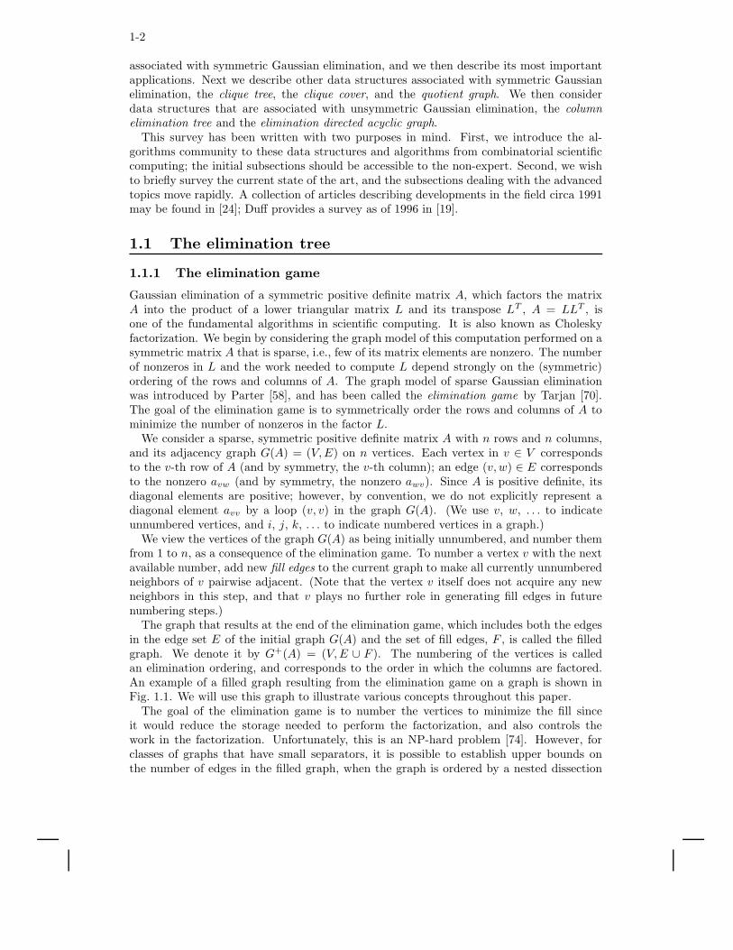
The graph that results at the end of the elimination game, which includes both the edgesin the edge set E of the initial graph G(A) and the set of fill edges, F , is called the filledgraph. We denote it by G+(A) = (V, E ∪ F ). The numbering of the vertices is calledan elimination ordering, and corresponds to the order in which the columns are factored.An example of a filled graph resulting from the elimination game on a graph is shown inFig. 1.1. We will use this graph to illustrate various concepts throughout this paper.

The goal of the elimination game is to number the vertices to minimize the fill sinceit would reduce the storage needed to perform the factorization, and also controls thework in the factorization. Unfortunately, this is an NP-hard problem [74]. However, forclasses of graphs that have small separators, it is possible to establish upper bounds onthe number of edges in the filled graph, when the graph is ordered by a nested dissection

Elimination Structures in Scientific Computing 1-3

1

25

4 3

6

1110

897

FIGURE 1.1: A filled graph G+(A) resulting from the elimination game on a graph G(A).The solid edges belong to G(A), and the broken edges are filled edges generated by theelimination game when vertices are eliminated in the order shown.

algorithm that recursively computes separators. Planar graphs, graphs of ‘well-shaped’finite element meshes (aspect ratios bounded away from small values), and overlap graphspossess elimination orderings with bounded fill. Conversely, the fill is large for graphs thatdo not have good separators.

Approximation algorithms that incur fill within a polylog factor of the optimum fill havebeen designed by Agrawal, Klein and Ravi [1]; but since it involves finding approximateconcurrent flows with uniform capacities, it is an impractical approach for large problems.A more recent approximation algorithm, due to Natanzon, Shamir and Sharan [57], limitsfill to within the square of the optimal value; this approximation ratio is better than thatof the former algorithm only for dense graphs.

The elimination game produces sets of cliques in the graph. Let hadj+(v) (ladj+(v))denote the higher-numbered (lower-numbered) neighbors of a vertex v in the graph G+(A);in the elimination game, hadj+(v) is the set of unnumbered neighbors of v immediatelyprior to the step in which v is numbered. When a vertex v is numbered, the set {v} ∪hadj+(v) becomes a clique by the rules of the elimination game. Future numbering stepsand consequent fill edges added do not change the adjacency set (in the filled graph) of thevertex v. (We will use hadj(v) and ladj(v) to refer to higher and lower adjacency sets of avertex v in the original graph G(A).)

1.1.2 The elimination tree data structure

We define a forest from the filled graph by defining the parent of a vertex v to be thelowest numbered vertex in hadj+(v). It is clear that this definition of parent yields a forestsince the parent of each vertex is numbered higher than itself. If the initial graph G(A) isconnected, then indeed we have a tree, the elimination tree; if not we have an eliminationforest.

In terms of the Cholesky factor L, the elimination tree is obtained by looking down each

1-4

11

10

6 9

8

7

5

42

31

FIGURE 1.2: The elimination tree of the example graph.

column below the diagonal element, and choosing the row index of the first subdiagonalnonzero to be the parent of a column. It will turn out that we can compute the eliminationtree corresponding to a matrix and a given ordering without first computing the filled graphor the Cholesky factor.

The elimination tree of the graph in Fig. 1.1 with the elimination ordering given there isshown in Fig. 1.2.

A fill path joining vertices i and j is a path in the original graph G(A) between verticesi and j, all of whose interior vertices are numbered lower than both i and j. The followingtheorem offers a static characterization of what causes fill in the elimination game.

THEOREM 1.1 [64] The edge (i, j) is an edge in the filled graph if and only if a fill pathjoins the vertices i and j in the original graph G(A).

In the example graph in Fig. 1.1, vertices 9 and 10 are joined a fill path consisting of theinterior vertices 7 and 8; thus (9, 10) is a fill edge. The next theorem shows that an edge inthe filled graph represents a dependence relation between its end points.

THEOREM 1.2 [69] If (i, j) is an edge in the filled graph and i < j, then j is an ancestorof the vertex i in the elimination tree T (A).

This theorem suggests that the elimination tree represents the information flow in theelimination game (and hence sparse symmetric Gaussian elimination). Each vertex i in-fluences only its higher numbered neighbors (the numerical values in the column i affectonly those columns in hadj+(i)). The elimination tree represents the information flow in aminimal way in that we need consider only how the information flows from i to its parentin the elimination tree. If j is the parent of i and ` is another higher neighbor of i, thensince the higher neighbors of i form a clique, we have an edge (j, `) that joins j and `; sinceby Theorem 1.2, ` is an ancestor of j, the information from i that affects ` can be viewedas being passed from i first to j, and then indirectly from j through its ancestors on thepath in the elimination tree to `.

An immediate consequence of the Theorem 1.2 is the following result.


COROLLARY 1.1 If vertices i and j belong to vertex-disjoint subtrees of the eliminationtree, then no edge can join i and j in the filled graph.

Viewing the dependence relationships in sparse Cholesky factorization by means of theelimination tree, we see that any topological reordering of the elimination tree would be anelimination ordering with the same fill, since it would not violate the dependence relation-ships. Such reorderings would not change the fill or arithmetic operations needed in thefactorization, but would change the schedule of operations in the factorization (i.e., whena specific operation is performed). This observation has been used in sparse matrix factor-izations to schedule the computations for optimal performance on various computationalplatforms: multiprocessors, hierarchical memory machines, external memory algorithms,etc. A postordering of the elimination tree is typically used to improve the spatial andtemporal data locality, and thereby the cache performance of sparse matrix factorizations.

There are two other perspectives from which we can view the elimination tree.Consider directing each edge of the filled graph from its lower numbered endpoint to

its higher numbered endpoint to obtain a directed acyclic graph (DAG). Now form thetransitive reduction of the directed filled graph; i.e., delete an edge (i, k) whenever there isa directed path from i to k that does not use the edge (i, k) (this path necessarily consistsof at least two edges since we do not admit multiple edges in the elimination game). Theminimal graph that remains when all such edges have been deleted is unique, and is theelimination tree.

One could also obtain the elimination tree by performing a depth-first search (DFS) inthe filled graph with the vertex numbered n as the initial vertex for the DFS, and choosingthe highest numbered vertex in ladj+(i) as the next vertex to search from a vertex i.

1.1.3 An algorithm

We begin with a consequence of the repeated application of the following fact: If a vertex iis adjacent to a higher numbered neighbor k in the filled graph, and k is not the parent ofi, pi, in the elimination tree, then i is adjacent to both k and pi in the filled graph; when iis eliminated, by the rules of the elimination game, a fill edge joins pi and k.

THEOREM 1.3 If (i, k) is an edge in the filled graph and i < k, then for every vertex jon an elimination tree path from i to k, (j, k) is also an edge in the filled graph.

This theorem leads to a characterization of ladj+(k), the set of lower numbered neighborsof a vertex k in the filled graph, which will be useful in designing an efficient algorithmfor computing the elimination tree. The set ladj+(k) corresponds to the column indices ofnonzeros in the k-th row of the Cholesky factor L, and ladj(k) corresponds to the columnindices of nonzeros in the lower triangle of the k-th row of the initial matrix A.

THEOREM 1.4 [51] Every vertex in the set ladj+(k) is a vertex reachable by paths inthe elimination tree from a set of leaves to k; each leaf l corresponds to a vertex in theset ladj(k) such that no proper descendant d of l in the elimination tree belongs to the setladj(k).

Theorem 1.4 characterizes the k-th row of the Cholesky factor L as a row subtree Tr(k)of the elimination subtree rooted at the vertex k, and pruned at each leaf l. The leavesof the pruned subtree are contained among ladj(k), the column indices of the nonzeros in(the lower triangle of) the k-th row of A. In the elimination tree in Fig. 1.2, the prunedelimination subtree corresponding to row 11 has two leaves, vertices 5 and 7; it includes allvertices on the etree path from these leaves to the vertex 11.

1-6

for k := 1 to n →pk := 0;for j ∈ ladj(k) (in increasing order) →

find the root r of the tree containing j;if (k 6= r) then k := pr; fi

rof

rof

FIGURE 1.3: An algorithm for computing an elimination tree. Initially each vertex is in asubtree with it as the root.

The observation above leads to an algorithm, shown in Fig. 1.3, for computing the elim-ination tree from the row structures of A, due to Liu [51].

This algorithm can be implemented efficiently using the union-find data structure fordisjoint sets. A height compressed version of the p. array, ancestor, makes it possible tocompute the root fast; and union by rank in merging subtrees helps to keep the merged treeshallow. The time complexity of the algorithm is O(eα(e, n) + n), where n is the numberof vertices and e is the number of edges in G(A), and α(e, n) is a functional inverse ofAckermann’s function. Liu [54] shows experimentally that path compression alone is moreefficient than path compression and union by rank, although the asymptotic complexityof the former is higher. Zmijewski and Gilbert [75] have designed a parallel algorithm forcomputing the elimination tree on distributed memory multiprocessors.

The concept of the elimination tree was implicit in many papers before it was formallyidentified. The term elimination tree was first used by Duff [17], although he studied aslightly different data structure; Schreiber [69] first formally defined the elimination tree,and its properties were established and used in several articles by Liu. Liu [54] also wrotean influential survey that delineated its importance in sparse matrix computations; we referthe reader to this survey for a more detailed discussion of the elimination tree current as of1990.

1.1.4 A skeleton graph

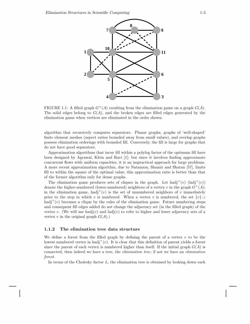
The filled graph represents a supergraph of the initial graph G(A), and a skeleton graphrepresents a subgraph of the latter. Many sparse matrix algorithms can be made moreefficient by implicitly identifying the edges of a skeleton graph G−(A) from the graphG(A) and an elimination ordering, and performing computations only on these edges. Askeleton graph includes only the edges that correspond to the leaves in each row subtree inTheorem 1.4. The other edges in the initial graph G(A) can be discarded, since they willbe generated as fill edges during the elimination game. Since each leaf of a row subtreecorresponds to an edge in G(A), the skeleton graph G−(A) is indeed a subgraph of theformer. The skeleton graph of the example graph is shown in Fig. 1.4.

The leaves in a row subtree can be identified from the set ladj(j) when the eliminationtree is numbered in a postordering. The subtree T (i) is the subtree of the elimination treerooted at a vertex i, and |T (i)| is the number of vertices in that subtree. (It should not beconfused with the row subtree Tr(i), which is a pruned subtree of the elimination tree.)

THEOREM 1.5 [51] Let ladj(j) = {i1 < i2 < . . . < is}, and let the vertices of a filledgraph be numbered in a postordering of its elimination tree T . Then vertex iq is a leaf of


1

25

4 3

6

1110

897

FIGURE 1.4: The skeleton graph G−(A) of the example graph.

the row subtree Tr(j) if and only if either q = 1, or for q ≥ 2, iq−1 < iq − |T (iq)| + 1.

1.1.5 Supernodes

A supernode is a subset of vertices S of the filled graph that form a clique and have the samehigher neighbors outside S. Supernodes play an important role in numerical algorithms sinceloops corresponding to columns in a supernode can be blocked to obtain high performanceon modern computer architectures. We now proceed to define a supernode formally.

A maximal clique in a graph is a set of vertices that induces a complete subgraph, butadding any other vertex to the set does not induce a complete subgraph. A supernode is amaximal clique {is, is+1, . . . , is+t−1} in a filled graph G+(A) such that for each 1 ≤ j ≤ t−1,

hadj+(is) = {is+1, . . . , is+j} ∪ hadj+(is+j).

Let hd+(is) ≡ |hadj+(is)|; since hadj+(is) ⊆ {is+1, . . . , is+j}∪hadj+(is+j), the relationshipbetween the higher adjacency sets can be replaced by the equivalent test on higher degrees:hd+(is) = hd+(is+j) + j.

In practice, fundamental supernodes, rather than the maximal supernodes defined above,are used, since the former are easier to work with in the numerical factorization. A fun-damental supernode is a clique but not necessarily a maximal clique, and satisfies twoadditional conditions: (1) is+j−1 is the only child of the vertex is+j in the elimination tree,for each 1 ≤ j ≤ t− 1; (2) the vertices in a supernode are ordered consecutively, usually bypost-ordering the elimination tree. Thus vertices in a fundamental supernode form a pathin the elimination tree; each of the non-terminal vertices in this path has only one child,and the child belongs to the supernode.

The fundamental supernodes corresponding to the example graph are: {1, 2}; {3, 4};{5, 6}; {7, 8, 9}; and {10, 11}.

Just as we could compute the elimination tree directly from G(A) without first computingG+(A), we can compute fundamental supernodes without computing the latter graph, usingthe theorem given below. Once the elimination tree is computed, this algorithm can be

1-8

implemented in O(n + e) time, where e ≡ |E| is the number of edges in the original graphG(A).

THEOREM 1.6 [56] A vertex i is the first node of a fundamental supernode if and onlyif i has two or more children in the elimination tree T , or i is a leaf of some row subtree ofT .

1.2 Applications of etrees

1.2.1 Efficient symbolic factorization

Symbolic factorization (or symbolic elimination) is a process that computes the nonzerostructure of the factors of a matrix without computing the numerical values of the nonzeros.

The symbolic Cholesky factor of a matrix has several uses. It is used to allocate the datastructure for the numeric factor and annotate it with all the row/column indices, whichenables the removal of most of the non-numeric operations from the inner-most loop of thesubsequent numeric factorization [20, 29]. It is also used to compute relaxed supernode (oramalgamated node) partitions, which group columns into supernodes even if they only haveapproximately the same structure [4, 21]. Symbolic factors can also be used in algorithmsthat construct approximate Cholesky factors by dropping nonzeros from a matrix A andfactoring the resulting, sparser matrix B [6, 72]. In such algorithms, elements of A thatare dropped from B but which appear in the symbolic factor of B can can be added to thematrix B; this improves the approximation without increasing the cost of factoring B. Inall of these applications a supernodal symbolic factor (but not a relaxed one) is sufficient;there is no reason to explicitly represent columns that are known to be identical.

The following algorithm for symbolically factoring a symmetric matrix A is due to Georgeand Liu [28] (and in a more graph-oriented form due to [64]; see also [29, Section 5.4.3]and [54, Section 8]).

The algorithm uses the elimination tree implicitly, but does not require it as input; thealgorithm can actually compute the elimination tree on the fly. The algorithm uses theobservation that

hadj+(j) = hadj(j)⋃

∪i,pi=j hadj+(i) .

That is, the structure of a column of L is the union of the structure of its children in theelimination tree and the structure of the same column in the lower triangular part of A.Identifying the children can be done using a given elimination tree, or the elimination treecan be constructed on the fly by adding column i to the list of children of pi when thestructure of i is computed (pi is the row index of the first subdiagonal nonzero in columni of L). The union of a set of column structures is computed using a boolean array P ofsize n (whose elements are all initialized to false), and an integer stack to hold the newlycreated structure. A row index k from a child column or from the column of A is added tothe stack only if P[k] = false. When row index k is added to the stack, P[k] is set to true tosignal that k is already in the stack. When the computation of hadj+(j) is completed, thestack is used to clear P so that it is ready for the next union operation. The total work inthe algorithm is Θ(|L|), since each nonzero requires constant work to create and constantwork to merge into the parent column, if there is a parent. (Here |L| denotes the number ofnonzeros in L, or equivalently the number of edges in the filled graph G+(A); similarly |A|denotes the number of nonzeros in A, or the number of edges in the initial graph G(A).)

The symbolic structure of the factor can usually be represented more compactly andcomputed more quickly by exploiting supernodes, since we essentially only need to represent


the identity of each supernode (the constituent columns) and the structure of the first (lowestnumbered) column in each supernode. The structure of any column can be computed fromthis information in time proportional to the size of the column. The George-Liu column-merge algorithm presented above can compute a supernodal symbolic factorization if it isgiven as input a supernodal elimination tree; such a tree can be computed in O(|A|) timeby the Liu-Ng-Peyton algorithm [56]. In practice, this approach saves a significant amountof work and storage.

Clearly, column-oriented symbolic factorization algorithms can also generate the structureof rows in the same asymptotic work and storage. But a direct symbolic factorizationby rows is less obvious. Whitten [73], in an unpublished manuscript cited by Tarjan andYannakakis [71], proposed a row-oriented symbolic factorization algorithm (see also [51] and[54, Sections 3.2 and 8.2]). The algorithm uses the characterization of the structure of rowi in L as the row subtree Tr(i). Given the elimination tree and the structure of A by rows,it is trivial to traverse the ith row subtree in time proportional to the number of nonzerosin row i of L. Hence, the elimination tree along with a row-oriented representation of A isan effective implicit symbolic row-oriented representation of L; an explicit representationis usually not needed, but it can be generated in work and space O(|L|) from this implicitrepresentation.

1.2.2 Predicting row and column nonzero counts

In some applications the explicit structure of columns of L is not required, only the numberof nonzeros in each column or each row. Gilbert, Ng, and Peyton [38] describe an almost-linear-time algorithm for determining the number of nonzeros in each row and column of L.Applications for computing these counts fast include comparisons of fill in alternative matrixorderings, preallocation of storage for a symbolic factorization, finding relaxed supernodepartitions quickly, determining the load balance in parallel factorizations, and determiningsynchronization events in parallel factorizations.

The algorithm to compute row counts is based on Whitten’s characterization [73]. Weare trying to compute |Li∗| = |Tr(i)|. The column indices j < i in row i of A define asubset of the vertices in the subtree of the elimination tree rooted at the vertex i, T [i].The difficulty, of course, is counting the vertices in Tr(i) without enumerating them. TheGilbert-Ng-Peyton algorithm counts these vertices using three relatively simple mechanisms:(1) processing the column indices j < i in row i of A in postorder of the etree, (2) computingthe distance of each vertex in the etree from the root, and (3) setting up a data structureto compute the least-common ancestor (LCA) of pairs of etree vertices. It is not hard toshow that the once these preprocessing steps are completed, |Tr(i)| can be computed using|Ai∗| LCA computations. The total cost of the preprocessing and the LCA computationsis almost linear in |A|.

Gilbert, Ng, and Peyton show how to further reduce the number of LCA computations.They exploit the fact that the leaves of Tr(i) are exactly the indices j that cause thecreation of new supernodes in the Liu-Ng-Peyton supernode-finding algorithm [56]. Thisobservation limits the LCA computations to leaves of row subtrees, i.e., edges in the skeletongraph G−(A). This significantly reduces the running time in practice.

Efficiently computing the column counts in L is more difficult. The Gilbert-Ng-Peytonalgorithm assigns a weight w(j) to each etree vertex j, such that |L∗j | =

∑

k∈T [j] w(k).Therefore, the column-count of a vertex is the sum of the column counts of its children, plusits own weight. Hence, wj must compensate for (1) the diagonal elements of the children,which are not included in the column count for j, (2) for rows that are nonzero in columnj but not in its children, and (3) for duplicate counting stemming from rows that appear

1-10

in more than one child. The main difficulty lies in accounting for duplicates, which is doneusing least-common-ancestor computations, as in the row-counts algorithm. This algorithm,too, benefits from handling only skeleton-graph edges.

Gilbert, Ng, and Peyton [38] also show in their paper how to optimize these algorithms,so that a single pass over the nonzero structure of A suffices to compute the row counts,the column counts, and the fundamental supernodes.

1.2.3 Three classes of factorization algorithms

There are three classes of algorithms used to implement sparse direct solvers: left-looking,right-looking, and multifrontal; all of them use the elimination tree to guide the compu-tation of the factors. The major difference between the first two of these algorithms isin how they schedule the computations they perform; the multifrontal algorithm organizescomputations differently from the other two, and we explain this after introducing someconcepts.

The computations on the sparse matrix are decomposed into subtasks involving compu-tations among dense submatrices (supernodes), and the precedence relations among themare captured by the supernodal elimination tree. The computation at each node of the elim-ination tree (subtask) involves the partial factorization of the dense submatrix associatedwith it.

The right-looking algorithm is an eager updating scheme: Updates generated by thesubmatrix of the current subtask are applied immediately to future subtasks that it islinked to by edges in the filled graph of the sparse matrix. The left-looking algorithm isa lazy updating scheme: Updates generated by previous subtasks linked to the currentsubtask by edges in the filled adjacency graph of the sparse matrix are applied just prior tothe factorization of the current submatrix. In both cases, updates always join a subtask tosome ancestor subtask in the elimination tree. In the multifrontal scheme, updates alwaysgo from a child task to its parent in the elimination tree; an update that needs to be appliedto some ancestor subtask is passed incrementally through a succession of vertices on theelimination tree path from the subtask to the ancestor.

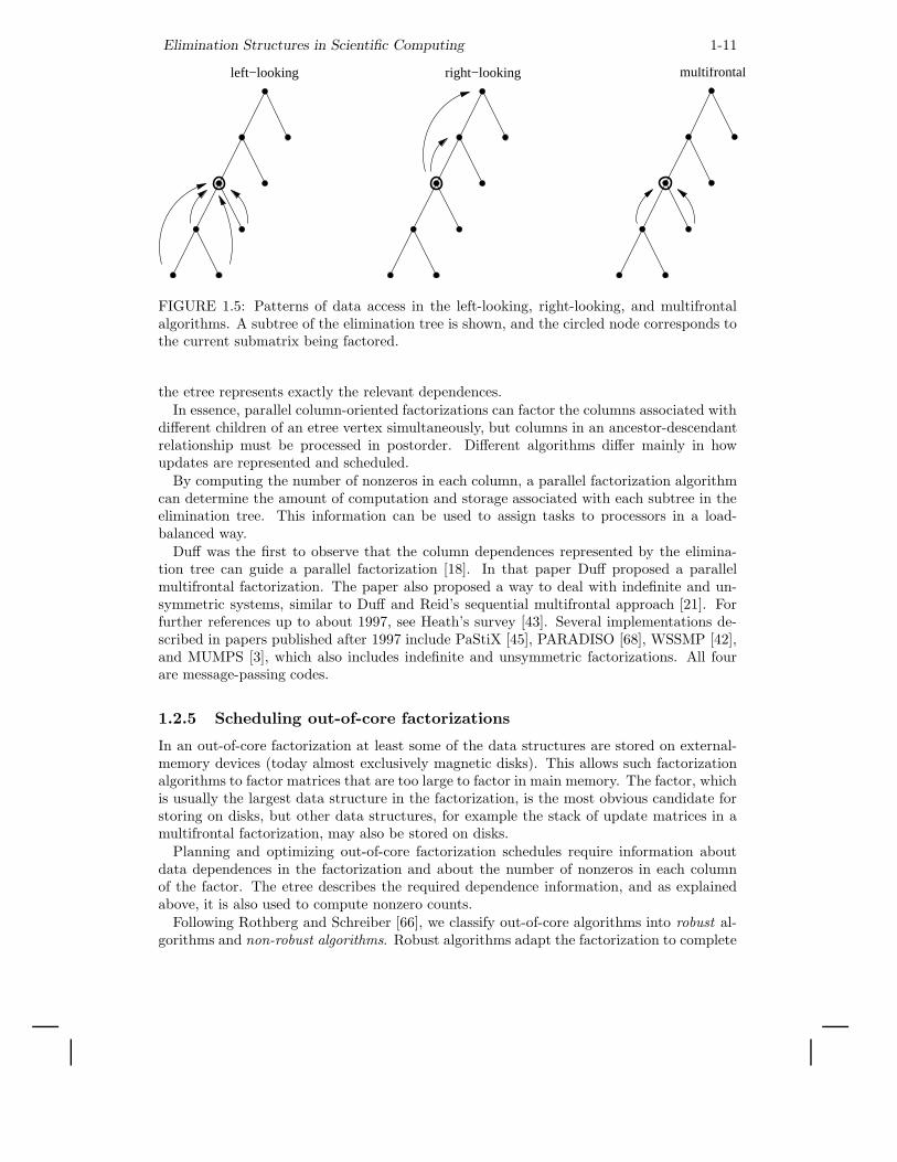
Thus the major difference among these three algorithms is how the data accesses andthe computations are organized and scheduled, while satisfying the precedence relationscaptured by the elimination tree. An illustration of these is shown in Fig. 1.5.

1.2.4 Scheduling parallel factorizations

In a parallel factorization algorithm, dependences between nonzeros in L determine the setof admissible schedules. A diagonal nonzero can only be factored after all updates to itfrom previous columns have been applied, a subdiagonal nonzero can be scaled only afterupdates to it have been applied (and after the diagonal element has been factored), andtwo subdiagonal nonzeros can update elements in the reduced system only after they havebeen scaled.

The elimination tree represents very compactly and conveniently a superset of thesedependences. More specifically, the etree represents dependences between columns of L. Acolumn can be completely factored only after all its descendants have been factored, and twocolumns that are not in an ancestor-descendant relationship can be factored in any order.Note that this is a superset of the element dependences, since a partially factored columncan already perform some of the updates to its ancestors. But most sparse eliminationalgorithms treat column operations (or row operations) as atomic operations that are alwaysperformed by a single processor sequentially and with no interruption. For such algorithms,


left−looking right−looking multifrontal

FIGURE 1.5: Patterns of data access in the left-looking, right-looking, and multifrontalalgorithms. A subtree of the elimination tree is shown, and the circled node corresponds tothe current submatrix being factored.

the etree represents exactly the relevant dependences.In essence, parallel column-oriented factorizations can factor the columns associated with

different children of an etree vertex simultaneously, but columns in an ancestor-descendantrelationship must be processed in postorder. Different algorithms differ mainly in howupdates are represented and scheduled.

By computing the number of nonzeros in each column, a parallel factorization algorithmcan determine the amount of computation and storage associated with each subtree in theelimination tree. This information can be used to assign tasks to processors in a load-balanced way.

Duff was the first to observe that the column dependences represented by the elimina-tion tree can guide a parallel factorization [18]. In that paper Duff proposed a parallelmultifrontal factorization. The paper also proposed a way to deal with indefinite and un-symmetric systems, similar to Duff and Reid’s sequential multifrontal approach [21]. Forfurther references up to about 1997, see Heath’s survey [43]. Several implementations de-scribed in papers published after 1997 include PaStiX [45], PARADISO [68], WSSMP [42],and MUMPS [3], which also includes indefinite and unsymmetric factorizations. All fourare message-passing codes.

1.2.5 Scheduling out-of-core factorizations

In an out-of-core factorization at least some of the data structures are stored on external-memory devices (today almost exclusively magnetic disks). This allows such factorizationalgorithms to factor matrices that are too large to factor in main memory. The factor, whichis usually the largest data structure in the factorization, is the most obvious candidate forstoring on disks, but other data structures, for example the stack of update matrices in amultifrontal factorization, may also be stored on disks.

Planning and optimizing out-of-core factorization schedules require information aboutdata dependences in the factorization and about the number of nonzeros in each columnof the factor. The etree describes the required dependence information, and as explainedabove, it is also used to compute nonzero counts.

Following Rothberg and Schreiber [66], we classify out-of-core algorithms into robust al-gorithms and non-robust algorithms. Robust algorithms adapt the factorization to complete

1-12

with the core memory available by performing the data movement and computations at asmaller granularity when necessary. They partition the submatrices corresponding to thesupernodes and stacks used in the factorization into smaller units called panels to ensurethat the factorization completes with the available memory. Non-robust algorithms assumethat the stack or a submatrix corresponding to a supernode fits within the core memoryprovided. In general, non-robust algorithms read elements of the input matrix only once,read from disk nothing else, and they only write the factor elements to disk; Dobrian andPothen refer to such algorithms as read-once-write-once, and to robust ones as read-many-write-many [15].

Liu proposed [53] a non-robust method that works as long as for all j = 1, . . . , n, all thenonzeros in the submatrix Lj:n,1:j of the factor fit simultaneously in main memory. Liu alsoshows in that paper how to reduce the amount of main memory required to factor a givenmatrix using this technique by reordering the children of vertices in the etree.

Rothberg and Schreiber [65, 66] proposed a number of robust out-of-core factorizationalgorithms. They proposed multifrontal, left-looking, and hybrid multifrontal/left-lookingmethods. Rotkin and Toledo [67] proposed two additional robust methods, a more efficientleft-looking method, and a hybrid right/left-looking method. All of these methods use theetree together with column-nonzero counts to organize the out-of-core factorization process.

Dobrian and Pothen [15] analyzed the amount of main memory required for read-once-write-once factorizations of matrices with several regular etree structures, and the amountof I/O that read-many-write-many factorizations perform on these matrices. They alsoprovided simulations on problems with irregular elimination tree structures. These studiesled them to conclude that an external memory sparse solver library needs to provide atleast two of the factorization methods, since each method can out-perform the others onproblems with different characteristics. They have provided implementations of out-of-core algorithms for all three of the multifrontal, left-looking, and right-looking factorizationmethods; these algorithms are included in the direct solver library OBLIO [16].

In addition to out-of-core techniques, there exist techniques that reduce the amount ofmain memory required to factor a matrix without using disks. Liu [52] showed how to min-imize the size of the stack of update matrices in the multifrontal method by reordering thechildren of vertices in the etree; this method is closely related to [53]. Another approach,first proposed by Eisenstat, Schultz and Sherman [23] uses a block factorization of the coef-ficient matrix, but drops some of the off-diagonal blocks. Dropping these blocks reduces theamount of main memory required for storing the partial factor, but requires recomputationof these blocks when linear systems are solved using the partial factor. George and Liu [29,Chapter 6] proposed a general algorithm to partition matrices into blocks for this technique.Their algorithm uses quotient graphs, data structures that we describe later in this chapter.

1.3 The clique tree

1.3.1 Chordal graphs and clique trees

The filled graph G+(A) that results from the elimination game on the matrix A (the adja-cency graph of the Cholesky factor L) is a chordal graph, i.e., a graph in which every cycleon four or more vertices has an edge joining two non-consecutive vertices on the cycle [63].(The latter edge is called a chord, whence the name chordal graph. This class of graphs hasalso been called triangulated or rigid circuit graphs.)

A vertex v in a graph G is simplicial if its neighbors adj(v) form a clique. Every chordalgraph is either a clique, or it has two non-adjacent simplicial vertices. (The simplicialvertices in the filled graph in Fig. 1.1 are 1, 2, 3, 4, 7, 8, and 9.) We can eliminate a simplicial


vertex v without causing any fill by the rules of the elimination game, since adj(v) is alreadya clique, and no fill edge needs to be added. A chordal graph from which a simplicial vertexis eliminated continues to be a chordal graph. A perfect elimination ordering of a chordalgraph is an ordering in which simplicial vertices are eliminated successively without causingany fill during the elimination game. A graph is chordal if and only if it has a perfectelimination ordering.

Suppose that the vertices of the adjacency graph G(A) of a sparse, symmetric matrixA have been re-numbered in an elimination ordering, and that G+(A) corresponds to thefilled graph obtained by the elimination game on G(A) with that ordering. This eliminationordering is a perfect elimination ordering of the filled graph G+(A). Many other perfectelimination orderings possible for G+(A), since there are at least two simplicial vertices thatcan be chosen for elimination at each step, until the graph has one uneliminated vertex.

It is possible to design efficient algorithms on chordal graphs whose time complexity ismuch less than O(|E ∪F |), where E ∪F denotes the set of edges in the chordal filled graph.This is accomplished by representing chordal graphs by tree data structures defined on themaximal cliques of the graph. (Recall that a clique K is maximal if K ∪ {v} is not a cliquefor any vertex v 6∈ K.)

THEOREM 1.7 Every maximal clique of a chordal filled graph G+(A) is of the formK(v) = {v} ∪ hadj+(v), with the vertices ordered in a perfect elimination ordering.

The vertex v is the lowest-numbered vertex in the maximal clique K(v), and is calledthe representative vertex of the clique. Since there can be at most n ≡ |V | representativevertices, a chordal graph can have at most n maximal cliques. The maximal cliques of thefilled graph in Fig. 1.1 are: K1 = {1, 2, 5, 10}; K2 = {3, 4, 5, 6}; K3 = {5, 6, 10, 11}; andK4 = {7, 8, 9, 10, 11}. The lowest-numbered vertex in each maximal clique is its represen-tative; note that in our notation K2 = K(3), K1 = K(1), K3 = K(5), and K4 = K(7).

Let KG = {K1, K2, . . . , Km} denote the set of maximal cliques of a chordal graph G.Define a clique intersection graph with the maximal cliques as its vertices, with two maximalcliques Ki and Kj joined by an edge (Ki, Kj) of weight |Ki∩Kj |. A clique tree correspondsto a maximum weight spanning tree (MST) of the clique intersection graph. Since the MSTof a weighted graph need not be unique, a clique tree of a chordal graph is not necessarilyunique either.

In practice, a rooted clique tree is used in sparse matrix computations. Lewis, Peyton,and Pothen [48] and Pothen and Sun [62] have designed algorithms for computing rootedclique trees. The former algorithm uses the adjacency lists of the filled graph as input,while the latter uses the elimination tree. Both algorithms identify representative verticesby a simple degree test. We will discuss the latter algorithm.

First, to define the concepts needed for the algorithm, consider that the the maximalcliques are ordered according to their representative vertices. This ordering partitions eachmaximal clique K(v) with representative vertex v into two subsets: new(K(v)) consists ofvertices in the clique K(v) whose higher adjacency sets are contained in it but not in anyearlier ordered maximal clique. The residual vertices in K(v)\new(K(v)) form the ancestorset anc(K(v)). If a vertex w ∈ anc(K(v)), by definition of the ancestor set, w has a higherneighbor that is not adjacent to v; then by the rules of the elimination game, any higher-numbered vertex x ∈ K(v) also belongs to anc(K(v)). Thus the partition of a maximalclique into new and ancestor sets is an ordered partition: vertices in new(K(v)) are orderedbefore vertices in anc(K(v)). We denote the lowest numbered vertex f in anc(K(v)) thefirst ancestor of the clique K(v). A rooted clique tree may be defined as follows: the parentof a clique K(v) is the clique P in which the first ancestor vertex f of K appears as a vertex

1-14

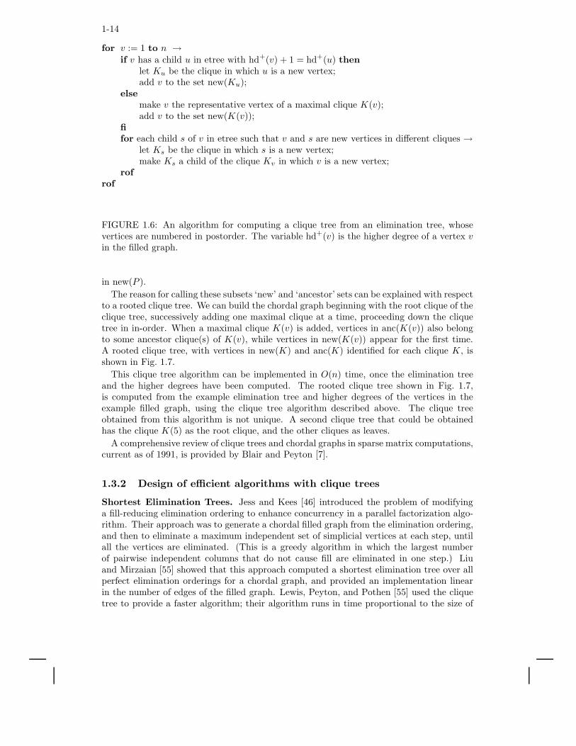
for v := 1 to n →if v has a child u in etree with hd+(v) + 1 = hd+(u) then

let Ku be the clique in which u is a new vertex;add v to the set new(Ku);

else

make v the representative vertex of a maximal clique K(v);add v to the set new(K(v));

fi

for each child s of v in etree such that v and s are new vertices in different cliques →let Ks be the clique in which s is a new vertex;make Ks a child of the clique Kv in which v is a new vertex;

rof

rof

FIGURE 1.6: An algorithm for computing a clique tree from an elimination tree, whosevertices are numbered in postorder. The variable hd+(v) is the higher degree of a vertex vin the filled graph.

in new(P ).

The reason for calling these subsets ‘new’ and ‘ancestor’ sets can be explained with respectto a rooted clique tree. We can build the chordal graph beginning with the root clique of theclique tree, successively adding one maximal clique at a time, proceeding down the cliquetree in in-order. When a maximal clique K(v) is added, vertices in anc(K(v)) also belongto some ancestor clique(s) of K(v), while vertices in new(K(v)) appear for the first time.A rooted clique tree, with vertices in new(K) and anc(K) identified for each clique K, isshown in Fig. 1.7.

This clique tree algorithm can be implemented in O(n) time, once the elimination treeand the higher degrees have been computed. The rooted clique tree shown in Fig. 1.7,is computed from the example elimination tree and higher degrees of the vertices in theexample filled graph, using the clique tree algorithm described above. The clique treeobtained from this algorithm is not unique. A second clique tree that could be obtainedhas the clique K(5) as the root clique, and the other cliques as leaves.

A comprehensive review of clique trees and chordal graphs in sparse matrix computations,current as of 1991, is provided by Blair and Peyton [7].

1.3.2 Design of efficient algorithms with clique trees

Shortest Elimination Trees. Jess and Kees [46] introduced the problem of modifyinga fill-reducing elimination ordering to enhance concurrency in a parallel factorization algo-rithm. Their approach was to generate a chordal filled graph from the elimination ordering,and then to eliminate a maximum independent set of simplicial vertices at each step, untilall the vertices are eliminated. (This is a greedy algorithm in which the largest numberof pairwise independent columns that do not cause fill are eliminated in one step.) Liuand Mirzaian [55] showed that this approach computed a shortest elimination tree over allperfect elimination orderings for a chordal graph, and provided an implementation linearin the number of edges of the filled graph. Lewis, Peyton, and Pothen [55] used the cliquetree to provide a faster algorithm; their algorithm runs in time proportional to the size of


�

7,8,9,10,11

10,11�

5,6

5,6�

3,4

5,10�

1,2

FIGURE 1.7: A clique tree of the example filled graph, computed from its elimination tree.Within each clique K in the clique tree, the vertices in new(K) are listed below the bar,and the vertices in anc(K) are listed above the bar.

the clique tree: the sum of the sizes of the maximal cliques of the chordal graph.

A vertex is simplicial if and only if it belongs to exactly one maximal clique in the chordalgraph; a maximum independent set of simplicial vertices is obtained by choosing one suchvertex from each maximal clique that contains simplicial vertices, and thus the clique treeis a natural data structure for this problem. The challenging aspect of the algorithm isto update the rooted clique tree when simplicial vertices are eliminated and cliques thatbecome non-maximal are absorbed by other maximal cliques.

Parallel Triangular Solution. In solving systems of linear equations by factorizationmethods, usually the work involved in the factorization step dominates the work involvedin the triangular solution step (although the communication costs and synchronizationoverheads of both steps are comparable). However, in some situations, many linear systemswith the same coefficient matrix but with different right-hand-side vectors need to be solved.In such situations, it is tempting to replace the triangular solution step involving the factormatrix L by explicitly computing an inverse L−1 of the factor. Unfortunately L−1 can bemuch less sparse than the factor, and so a more space efficient ‘product-form inverse’ needsto be employed. In this latter form, the inverse is represented as a product of triangularmatrices such that all the matrices in the product together require exactly as much spaceas the original factor.

The computation of the product form inverse leads to some interesting chordal graphpartitioning problems that can be solved efficiently by using a clique tree data structure.

We begin by directing each edge in the chordal filled graph G+(A) from its lower to itshigher numbered end point to obtain a directed acyclic graph (DAG). We will denote thisDAG by G(L). Given an edge (i, j) directed from i to j, we will call i the predecessor of j,and j the successor of i. The elimination ordering must eliminate vertices in a topological

1-16

ordering of the DAG such that all predecessors of a vertex must be eliminated before it canbe eliminated. The requirement that each matrix in the product form of the inverse musthave the same nonzero structure as the corresponding columns in the factor is expressed bythe fact that the subgraph corresponding to the matrix should be transitively closed. (Adirected graph is transitively closed if whenever there is a directed path from a vertex i toa vertex j, there is an edge directed from i to j in the graph.) Given a set of vertices Pi,the column subgraph of Pi includes all the vertices in Pi and vertices reached by directededges leaving vertices in Pi; the edges in this subgraph include all edges with one or bothendpoints in Pi.

The simpler of the graph partitioning problems is the following:Find an ordered partition P1 ≺ P2 ≺ . . . Pm of the vertices of a directed acyclic filled graphG(L) such that1. every v ∈ Pi has all of its predecessors included in P1, . . ., Pi;2. the column subgraph of Pi is transitively closed; and3. the number of subgraphs m is minimum over all topological orderings of G(L).

Pothen and Alvarado [61] designed a greedy algorithm that runs in O(n) time to solvethis partitioning problem by using the elimination tree.

A more challenging variant of the problem minimizes the number of transitively closedsubgraphs in G(L) over all perfect elimination orderings of the undirected chordal filledgraph G+(A). This variant could change the edges in the DAG G(L), (but not the edgesin G+(A)) since the initial ordering of the vertices is changed by the perfect eliminationordering, and after the reordering, edges are directed from the lower numbered end pointto its higher numbered end point.

This is quite a difficult problem, but two surprisingly simple greedy algorithms solveit. Peyton, Pothen, and Yuan provide two different algorithms for this problem; the firstalgorithm uses the elimination tree and runs in time linear in the number of edges in thefilled graph [59]. The second makes use of the clique tree, and computes the partition intime linear in the size of the clique tree [60]. Proving the correctness of these algorithmsrequires a careful study of the properties of the minimal vertex separators (these are verticesin the intersections of the maximal cliques) in the chordal filled graph.

1.3.3 Compact clique trees

In analogy with skeleton graphs, we can define a space-efficient version of a clique treerepresentation of a chordal graph, called the compact clique tree. If K is the parent cliqueof a clique C in a clique tree, then it can be shown that anc(C) ⊂ K. Thus trading spacefor computation, we can delete the vertices in K that belong to the ancestor sets of itschildren, since we can recompute them when necessary by unioning the ancestor sets of thechildren. The partition into new and ancestor sets can be obtained by storing the lowestnumbered ancestor vertex for each clique. A compact clique Kc corresponding to a cliqueK is:

Kc = K \ ∪C∈child(K)anc(C).

Note that the compact clique depends on the specific clique tree from which it is computed.A compact clique tree is obtained from a clique tree by replacing cliques by compact

cliques for vertices. In the example clique tree, the compact cliques of the leaves are un-changed from the corresponding cliques; and the compact cliques of the interior cliques areKc(5) = {11}, and Kc(7) = {7, 8, 9}.

The compact clique tree is potentially sparser (asymptotically O(n) instead of O(n2)even) than the skeleton graph on pathological examples, but on “practical” examples, the


size difference between them is small. Compact clique trees were introduced by Pothen andSun [62].

1.4 Clique covers and quotient graphs

Clique covers and quotient graphs are data structures that were developed for the efficientimplementation of minimum-degree reordering heuristics for sparse matrices. In Gaussianelimination, an elimination step that uses aij as a pivot (the elimination of the jth un-known using the ith equation) modifies every coefficient akl for which akj 6= 0 and ail 6= 0.Minimum-degree heuristics attempt to select pivots for which the number of modified coef-ficients is small.

1.4.1 Clique covers

Recall the graph model of symmetric Gaussian elimination discussed in subsection 1.1.1.The adjacency graph of the matrix to be factored is an undirected graph G = (V, E),V = {1, 2, . . . , n}, E = {(i, j) : aij 6= 0}. The elimination of a row/column j correspondsto eliminating vertex j and adding edges to the remaining graph so that the neighbors ofj become a clique. If we represent the edge set E using a clique cover, a set of cliquesK = {K : K ⊆ V } such that E = ∪K∈K{(i, j) : i, j ∈ K}, the vertex elimination processbecomes a process of merging cliques [63]: The elimination of vertex j corresponds tomerging all the cliques that j belongs to into one clique and removing j from all the cliques.Clearly, all the old cliques that j used to belong to are now covered by the new clique, sothey can be removed from the cover. The clique-cover can be initialized by representingevery nonzero of A by a clique of size 2. This process corresponds exactly to symbolicelimination, which we have discussed in Section 1.2, and which costs Θ(|L|) work. Thecliques correspond exactly to frontal matrices in the multifrontal factorization method.

In the sparse-matrix literature, this model of Gaussian elimination has been sometimescalled the generalized-element model or the super-element model, due to its relationship tofinite-element models and matrices.

The significance of clique covers is due to the fact that in minimum-degree ordering codes,there is no need to store the structure of the partially computed factor, so when one cliqueis merged into another, it can indeed be removed from the cover. This implies that the totalsize

∑

K∈K |K| of the representation of the clique cover, which starts at exactly |A| − n,shrinks in every elimination step, so it is always bounded by |A| − n. Since exactly oneclique is formed in every elimination step, the total number of cliques is also bounded, byn + (|A| − n) = |A|. In contrast, the storage required to explicitly represent the symbolicfactor, or even to just explicitly represent the edges in the reduced matrix, can grow inevery elimination step and is not bounded by O(|A|).

Some minimum-degree codes represent cliques fully explicitly [8, 36]. This representationuses an array of cliques and an array of vertices; each clique is represented by a linked listof vertex indices, and each vertex is represented by a linked list of clique indices to which itbelongs. The size of this data structure never grows—linked-list elements are moved fromone list to another or are deleted during elimination steps, but new elements never need tobe allocated once the data structure is initialized.

Most codes, however, use a different representation for clique covers, which we describenext.

1-18

1.4.2 Quotient graphs

Most minimum-degree codes represent the graphs of reduced matrices during the eliminationprocess using quotient graphs [25]. Given a graph G = (V, E) and a partition S of Vinto disjoint sets Sj ∈ S, the quotient graph G/S is the undirected graph (S, E) whereE = {(Si,Sj) : adj(Si) ∩ Sj 6= ∅}.

The representation of a graph G after the elimination of vertices 1, 2, . . . , j − 1, butbefore the elimination of vertex j, uses a quotient graph G/S, where S consists of sets Sk

of eliminated vertices that form maximal connected components in G, and sets Si = {i} ofuneliminated vertices i ≥ j. We denote a set Sk of eliminated vertices by the index k of thehighest-numbered vertex in it.

This quotient graph representation of an elimination graph corresponds to a clique coverrepresentation as follows. Each edge in the quotient graph between uneliminated verticesS{i1} and S{i2} corresponds to a clique of size 2; all the neighbors of an eliminated set Sk

correspond to a clique, the clique that was created when vertex k was eliminated. Note thatall the neighbors of an uneliminated set Sk are uneliminated vertices, since uneliminatedsets are maximal with respect to connectivity in G.

The elimination of vertex j in the quotient-graph representation corresponds to markingSj as eliminated and merging it with its eliminated neighbors, to maintain the maximalconnectivity invariant.

Clearly, a representation of the initial graph G using adjacency lists is also a representationof the corresponding quotient graph. George and Liu [26] show how to maintain the quotientgraph efficiently using this representation without allocating more storage through a seriesof elimination steps.

Most of the codes that implement minimum-degree ordering heuristics, such as GEN-MMD [50], AMD [2], and Spindle [14, 47], use quotient graphs to represent eliminationgraphs.

It appears that the only advantage of a quotient graph over an explicit clique cover inthe context of minimum-degree algorithms is a reduction by a small constant factor inthe storage requirement, and possibly in the amount of work required. Quotient graphs,however, can also represent symmetric partitions of symmetric matrices in applications thatare not directly related to elimination graphs. For example, George and Liu use quotientgraphs to represent partitions of symmetric matrices into block matrices that can be factoredwithout fill in blocks that only contain zeros [29, Chapter 6].

In [27], George and Liu showed how to implement the minimum degree algorithm withoutmodifying the representation of the input graph at all. In essence, this approach representsthe quotient graph implicitly using the input graph and the indices of the eliminated vertices.The obvious drawback of this approach is that vertex elimination (as well as other requiredoperations) are expensive.

1.4.3 The problem of degree updates

The minimum-degree algorithm works by repeatedly eliminating the vertex with the min-imum degree and turning its neighbors into a clique. If the reduced graph is representedby a clique cover or a quotient graph, then the representation does not reveal the degreeof vertices. Therefore, when a vertex is eliminated from a graph represented by a cliquecover or a quotient graph, the degrees of its neighbors must be recomputed. These degreeupdates can consume much of the running time of minimum-degree algorithms.

Practical minimum-degree codes use several techniques to address this issue. Some tech-niques reduce the running time while preserving the invariant that the vertex that is elim-


inated always has the minimum degree. For example, mass elimination, the elimination ofall the vertices of a supernode consecutively without recomputing degrees, can reduce therunning time significantly without violating this invariant. Other techniques, such as mul-tiple elimination and the use of approximate degrees, do not preserve the minimum-degreeinvariant. This does not imply that the elimination orderings that such technique produceare inferior to true minimum-degree orderings. They are often superior to them. This is nota contradiction since the minimum-degree rule is just a heuristic which is rarely optimal.For further details, we refer the reader to George and Liu’s survey [30], to Amestoy, Davis,and Duff’s paper on approximate minimum-degree rules [2], and to Kumfert and Pothen’swork on minimum-degree variants [14, 47]. Heggernes, Eisenstat, Kumfert and Pothenprove upper bounds on the running time of space-efficient minimum-degree variants [44].

1.4.4 Covering the column-intersection graph and biclique covers

Column orderings for minimizing fill in Gaussian elimination with partial pivoting and in theorthogonal-triangular (QR, where Q is an orthogonal matrix, and R is an upper triangularmatrix) factorization are often based on symmetric fill minimization in the symmetric factorof AT A, whose graph is known as the the column intersection graph G∩(A) (we ignore thepossibility of numerical cancellation in AT A). To run a minimum-degree algorithm on thecolumn intersection graph, a clique cover or quotient graph of it must be constructed. Oneobvious solution is to explicitly compute the edge-set of G∩(A), but this is inefficient, sinceG∩(A) can be much denser than G(A).

A better solution is to initialize the clique cover using a clique for every row of A; thevertices of the clique are the indices of the nonzeros in that row [30]. It is easy to seethat each row in A indeed corresponds to a clique in G∩(A). This approach is used in theCOLMMD routine in Matlab [36] and in COLAMD [11].

A space-efficient quotient-graph representation for G∩(A) can be constructed by creatingan adjacency-list representation of the symmetric 2-by-2 block matrix

(

I AAT 0

)

and eliminating vertices 1 through n. The graph of the Schur complement matrix

G(0 − AT I(−1)A) = G(AT A) = G∩(A).

If we maintain a quotient-graph representation of the reduced graph through the first nelimination steps, we obtain a space-efficient quotient graph representation of the column-intersection graph. This is likely to be more expensive, however, than constructing theclique-cover representation from the rows of A. We learned of this idea from John Gilbert;we are not aware of any practical code that uses it.

The nonzero structure of the Cholesky factor of AT A is only an upper bound on thestructure of the LU factors in Gaussian elimination with partial pivoting. If the identitiesof the pivots are known, the nonzero structure of the reduced matrices can be representedusing biclique covers. The nonzero structure of A is represented by a bipartite graph({1, 2, . . . , n} ∪ {1′, 2′, . . . , n′}, {(i, j′) : aij 6= 0}). A biclique is a complete bipartite graphon a subset of the vertices. Each elimination step corresponds to a removal of two connectedvertices from the bipartite graph, and an addition of a new biclique. The vertices of the newbiclique are the neighbors of the two eliminated vertices, but they are not the union of a setof bicliques. Hence, the storage requirement of this representation may exceed the storagerequired for the initial representation. Still, the storage requirement is always smaller

1-20

than the storage required to represent each edge of the reduced matrix explicitly. Thisrepresentation poses the same degree update problem that symmetric clique covers pose,and the same techniques can be used to address it. Version 4 of UMFPACK, an unsymmetricmultifrontal LU factorization code, uses this idea together with a degree approximationtechnique to select pivots corresponding to relatively sparse rows in the reduced matrix [9].

1.5 Column elimination trees and elimination DAGS

Elimination structures for unsymmetric Gaussian elimination are somewhat more complexthan the equivalent structures for symmetric elimination. The additional complexity arisesbecause of two issues. First, the factorization of a sparse unsymmetric matrix A, where Ais factored into a lower triangular factor L and an upper triangular factor U , A = LU is lessstructured than the sparse symmetric factorization process. In particular, the relationshipbetween the nonzero structure of A and the nonzero structure of the factors is much morecomplex. Consequently, data structures for predicting fill and representing data-flow andcontrol-flow dependences in elimination algorithms are more complex and more diverse.

Second, factoring an unsymmetric matrix often requires pivoting, row and/or columnexchanges, to ensure existence of the factors and numerical stability. For example, the2-by-2 matrix A = [0 1; 1 0] does not have an LU factorization, because there is no wayto eliminate the first variable from the first equation: that variable does not appear inthe equation at all. But the permuted matrix PA does have a factorization, if P is apermutation matrix that exchanges the two rows of A. In finite precision arithmetic, rowand/or column exchanges are necessary even when a nonzero but small diagonal element isencountered. Some sparse LU algorithms perform either row or column exchanges, but notboth. The two cases are essentially equivalent (we can view one as a factorization of AT ),so we focus on row exchanges (partial pivoting). Other algorithms, primarily multifrontalalgorithms, perform both row and column exchanges; these are discussed toward the end ofthis section.

For completeness, we note that pivoting is also required in the factorization of sparsesymmetric indefinite matrices. Such matrices are usually factored into a product LDLT ,where L is lower triangular and D is a block diagonal matrix with 1-by-1 and 2-by-2 blocks.There has not been much research about specialized elimination structures for these fac-torization algorithms; such codes invariably use the symmetric elimination tree of A torepresent dependences for structure prediction and for scheduling the factorization.

The complexity and diversity of unsymmetric elimination arises not only due to pivoting,but also because unsymmetric factorizations are less structured than symmetric ones, soa rooted tree can no longer represent the factors. Instead, directed acyclic graphs (dags)are used to represent the factors and dependences in the elimination process. We discusselimination dags (edags) in Section 1.5.2.

Surprisingly, dealing with partial pivoting turns out to be simpler than dealing with theunsymmetry, so we focus next on the column elimination tree, an elimination structure forLU factorization with partial pivoting.

1.5.1 The column elimination tree

The column elimination tree (col-etree) is the elimination tree of AT A, under the assumptionthat no numerical cancelation occurs in the formation of AT A. The significance of this treeto LU with partial pivoting stems from a series of results that relate the structure of theLU factors of PA, where P is some permutation matrix, to the structure of the Cholesky


1

25

4 3

6

1110

897

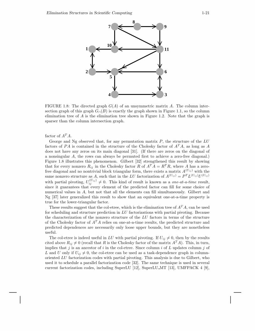
FIGURE 1.8: The directed graph G(A) of an unsymmetric matrix A. The column inter-section graph of this graph G∩(B) is exactly the graph shown in Figure 1.1, so the columnelimination tree of A is the elimination tree shown in Figure 1.2. Note that the graph issparser than the column intersection graph.

factor of AT A.

George and Ng observed that, for any permutation matrix P , the structure of the LUfactors of PA is contained in the structure of the Cholesky factor of AT A, as long as Adoes not have any zeros on its main diagonal [31]. (If there are zeros on the diagonal ofa nonsingular A, the rows can always be permuted first to achieve a zero-free diagonal.)Figure 1.8 illustrates this phenomenon. Gilbert [32] strengthened this result by showingthat for every nonzero Rij in the Cholesky factor R of AT A = RT R, where A has a zero-free diagonal and no nontrivial block triangular form, there exists a matrix A(Uij ) with thesame nonzero structure as A, such that in the LU factorization of A(Uij ) = P T L(Uij)U (Uij)

with partial pivoting, U(Uij)ij 6= 0. This kind of result is known as a one-at-a-time result,

since it guarantees that every element of the predicted factor can fill for some choice ofnumerical values in A, but not that all the elements can fill simultaneously. Gilbert andNg [37] later generalized this result to show that an equivalent one-at-a-time property istrue for the lower-triangular factor.

These results suggest that the col-etree, which is the elimination tree of AT A, can be usedfor scheduling and structure prediction in LU factorizations with partial pivoting. Becausethe characterization of the nonzero structure of the LU factors in terms of the structureof the Cholesky factor of AT A relies on one-at-a-time results, the predicted structure andpredicted dependences are necessarily only loose upper bounds, but they are nonethelessuseful.

The col-etree is indeed useful in LU with partial pivoting. If Uij 6= 0, then by the resultscited above Rij 6= 0 (recall that R is the Cholesky factor of the matrix AT A). This, in turn,implies that j is an ancestor of i in the col-etree. Since column i of L updates column j ofL and U only if Uij 6= 0, the col-etree can be used as a task-dependence graph in column-oriented LU factorization codes with partial pivoting. This analysis is due to Gilbert, whoused it to schedule a parallel factorization code [32]. The same technique is used in severalcurrent factorization codes, including SuperLU [12], SuperLU MT [13], UMFPACK 4 [9],

1-22

and TAUCS [40, 5]. Gilbert and Grigori [33] recently showed that this characterization istight in a strong all-at-once sense: for every strong Hall matrix A (i.e., A has no nontrivialblock-triangular form), there exists a permutation matrix P such that every edge of thecol-etree corresponds to a nonzero in the upper-triangular factor of PA. This implies thatthe a-priori symbolic column-dependence structure predicted by the col-etree is as tight aspossible.

Like the etree of a symmetric matrix, the col-etree can be computed in time almost linearin the number of nonzeros in A [34]. This is done by an adaptation of the symmetric etreealgorithm, an adaptation that does not compute explicitly the structure of AT A. Insteadof constructing G(AT A), the algorithm constructs a much sparser graph G′ with the sameelimination tree. The main idea is that each row of A contributes a clique to G(AT A); thismeans that each nonzero index in the row must be an ancestor of the preceding nonzeroindex. A graph in which this row-clique is replaced by a path has the same eliminationtree, and it has only as many edges as there are nonzeros in A. The same paper showsnot only how to compute the col-etree in almost linear time, but also how to bound thenumber of nonzeros in each row and column of the factors L and U , using again an extensionof the symmetric algorithm to compute the number of nonzeros in the Cholesky factor ofAT A. The decomposition of this Cholesky factor into fundamental supernodes, which thealgorithm also computes, can be used to bound the extent of fundamental supernodes thatwill arise in L.

1.5.2 Elimination DAGS

The col-etree represents all possible column dependences for any sequence of pivot rows. Fora specific sequence of pivots, the col-etree includes dependences that do not occur duringthe factorization with these pivots. There are two typical situations in which the pivotingsequence is known. The first is when the matrix is known to have a stable LU factorizationwithout pivoting. The most common case is when AT is strictly diagonally dominant. Evenif A is not diagonally dominant, its rows can be pre-permuted to bring large elements to thediagonal. The permuted matrix, even if its transpose is not diagonally dominant, is fairlylikely to have a relatively stable LU factorization that can be used to accurately solve linearsystems of equations. This strategy is known as static pivoting [49]. The other situation inwhich the pivoting sequence is known is when the matrix, or part of it, has already beenfactored. Since virtually all sparse factorization algorithms need to collect information fromthe already-factored portion of the matrix before they factor the next row and column, acompact representation of the structure of this portion is useful.

Elimination dags (edags) are directed acyclic graphs that capture a minimal or nearminimal set of dependences in the factors. Several edags have been proposed in the liter-ature. There are two reasons for this diversity. First, edags are not always as sparse andeasy to compute as elimination trees, so researchers have tried to find edags that are easy tocompute, even if they represent a superset of the actual dependences. Second, edags oftencontains information only about a specific structure in the factors or a specific dependencein a specific elimination algorithm (e.g., data dependence in a multifrontal algorithm), sodifferent edags are used for different applications. In other words, edags are not as universalas etrees in their applications.

The simplest edag is the graph G(LT ) of the transpose of the lower triangular factor, ifwe view every edge in this graph as directed from the lower-numbered vertex to a higher-numbered vertex. This corresponds to orienting edges from a row index to a column indexin L. For example, if L6,3 6= 0, we view the edge (6, 3) as a directed edge 3 → 6 in G(LT ).Let us denote by G((L(j−1))T ) the partial lower triangular factor after j − 1 columns have


1

25

4 3

6

1110

897

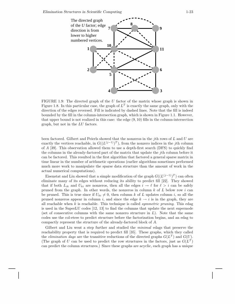
The directed graph of the U factor; edge direction is from lower to higher numbered vertices.

FIGURE 1.9: The directed graph of the U factor of the matrix whose graph is shown inFigure 1.8. In this particular case, the graph of LT is exactly the same graph, only with thedirection of the edges reversed. Fill is indicated by dashed lines. Note that the fill is indeedbounded by the fill in the column-intersection graph, which is shown in Figure 1.1. However,that upper bound is not realized in this case: the edge (9, 10) fills in the column-intersectiongraph, but not in the LU factors.

been factored. Gilbert and Peierls showed that the nonzeros in the jth rows of L and U areexactly the vertices reachable, in G((L(j−1))T ), from the nonzero indices in the jth columnof A [39]. This observation allowed them to use a depth-first search (DFS) to quickly findthe columns in the already-factored part of the matrix that update the jth column before itcan be factored. This resulted in the first algorithm that factored a general sparse matrix intime linear in the number of arithmetic operations (earlier algorithms sometimes performedmuch more work to manipulate the sparse data structure than the amount of work in theactual numerical computations).

Eisenstat and Liu showed that a simple modification of the graph G((L(j−1))T ) can ofteneliminate many of its edges without reducing its ability to predict fill [22]. They showedthat if both Lik and Uki are nonzeros, then all the edges i → ` for ` > i can be safelypruned from the graph. In other words, the nonzeros in column k of L below row i canbe pruned. This is true since if Uki 6= 0, then column k of L updates column i, so all thepruned nonzeros appear in column i, and since the edge k → i is in the graph, they areall reachable when k is reachable. This technique is called symmetric pruning. This edagis used in the SuperLU codes [12, 13] to find the columns that update the next supernode(set of consecutive columns with the same nonzero structure in L). Note that the samecodes use the col-etree to predict structure before the factorization begins, and an edag tocompactly represent the structure of the already-factored block of A.

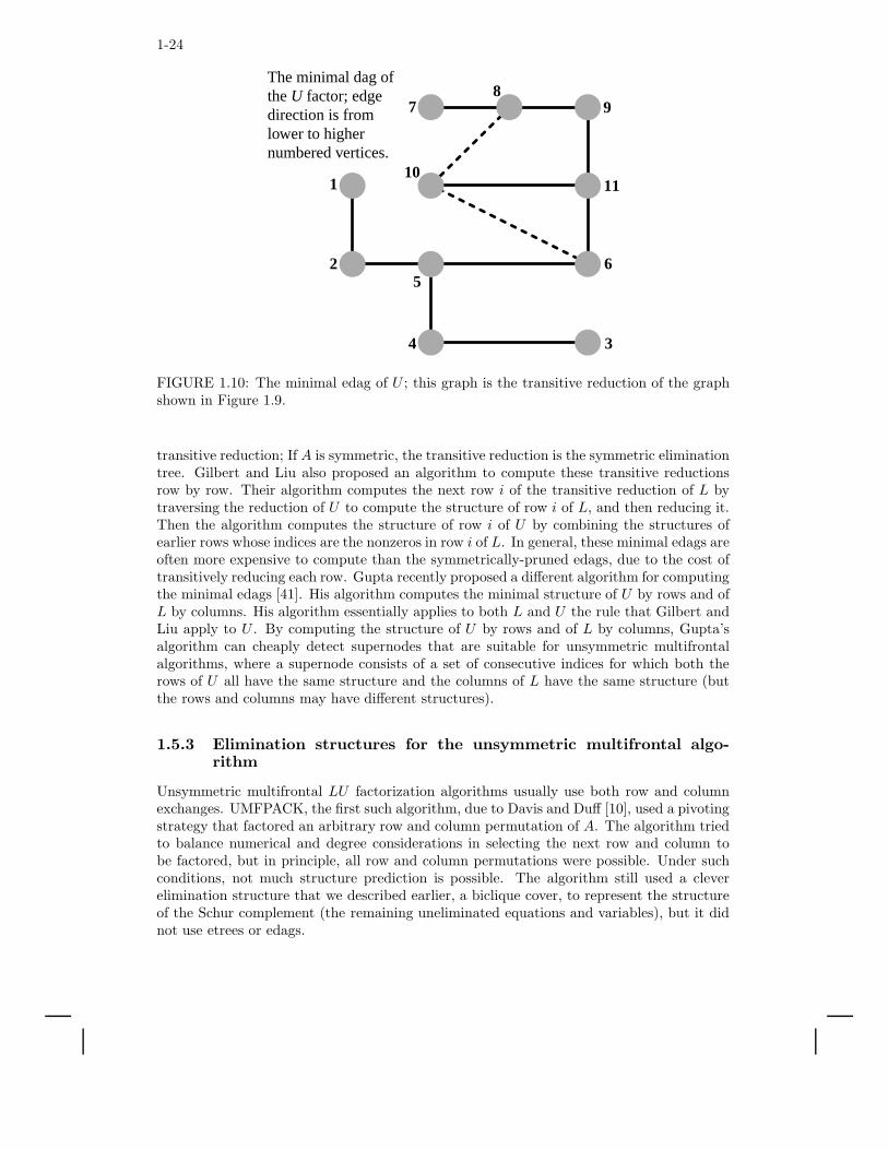
Gilbert and Liu went a step further and studied the minimal edags that preserve thereachability property that is required to predict fill [35]. These graphs, which they calledthe elimination dags are the transitive reductions of the directed graphs G(LT ) and G(U).(The graph of U can be used to predict the row structures in the factors, just as G(LT )can predict the column structures.) Since these graphs are acyclic, each graph has a unique

1-24

1

25

4 3

6

1110

897

The minimal dag of the U factor; edge direction is from lower to higher numbered vertices.

FIGURE 1.10: The minimal edag of U ; this graph is the transitive reduction of the graphshown in Figure 1.9.

transitive reduction; If A is symmetric, the transitive reduction is the symmetric eliminationtree. Gilbert and Liu also proposed an algorithm to compute these transitive reductionsrow by row. Their algorithm computes the next row i of the transitive reduction of L bytraversing the reduction of U to compute the structure of row i of L, and then reducing it.Then the algorithm computes the structure of row i of U by combining the structures ofearlier rows whose indices are the nonzeros in row i of L. In general, these minimal edags areoften more expensive to compute than the symmetrically-pruned edags, due to the cost oftransitively reducing each row. Gupta recently proposed a different algorithm for computingthe minimal edags [41]. His algorithm computes the minimal structure of U by rows and ofL by columns. His algorithm essentially applies to both L and U the rule that Gilbert andLiu apply to U . By computing the structure of U by rows and of L by columns, Gupta’salgorithm can cheaply detect supernodes that are suitable for unsymmetric multifrontalalgorithms, where a supernode consists of a set of consecutive indices for which both therows of U all have the same structure and the columns of L have the same structure (butthe rows and columns may have different structures).

1.5.3 Elimination structures for the unsymmetric multifrontal algo-rithm

Unsymmetric multifrontal LU factorization algorithms usually use both row and columnexchanges. UMFPACK, the first such algorithm, due to Davis and Duff [10], used a pivotingstrategy that factored an arbitrary row and column permutation of A. The algorithm triedto balance numerical and degree considerations in selecting the next row and column tobe factored, but in principle, all row and column permutations were possible. Under suchconditions, not much structure prediction is possible. The algorithm still used a cleverelimination structure that we described earlier, a biclique cover, to represent the structureof the Schur complement (the remaining uneliminated equations and variables), but it didnot use etrees or edags.


Recent unsymmetric multifrontal algorithms still use pivoting strategies that allow bothrow and column exchanges, but the pivoting strategies are restricted enough that struc-ture prediction is possible. These pivoting strategies are based on delayed pivoting, whichwas originally invented for symmetric indefinite factorizations. One such code, Davis’sUMFPACK 4, uses the column elimination tree to represent control-flow dependences, anda biclique cover to represent data dependences [9]. Another code, Gupta’s WSMP, usesconventional minimal edags to represent control-flow dependences, and specialized dags torepresent data dependences [41]. More specifically, Gupta shows how to modify the min-imal edags so they exactly represent data dependences in the unsymmetric multifrontalalgorithm with no pivoting, and how to modify the edags to represent dependences in anunsymmetric multifrontal algorithm that employs delayed pivoting.

Acknowledgment

Alex Pothen was supported, in part, by the National Science Foundation under grant CCR-0306334, and by the Department of Energy under subcontract DE-FC02-01ER25476. SivanToledo was supported in part by an IBM Faculty Partnership Award, by grant 572/00 fromthe Israel Science Foundation (founded by the Israel Academy of Sciences and Humanities),and by Grant 2002261 from the US-Israeli Binational Science Foundation.

References

References

[1] Ajit Agrawal, Philip Klein, and R. Ravi. Cutting down on fill using nested dissection:

Provably good elimination orderings. In [24], pages 31–55, 1993.

[2] Patrick R. Amestoy, Timothy A. Davis, and Iain S. Duff. An approximate minimum

degree ordering algorithm. SIAM Journal on Matrix Analysis and Applications,17(4):886–905, 1996.

[3] Patrick R. Amestoy, Iain S. Duff, Jean-Yves L’Excellent, and Jacko Koster. A fully

asynchronous multifrontal solver using distributed dynamic scheduling. SIAM Journalon Matrix Analysis and Applications, 23(1):15–41, 2001.

[4] Cleve Ashcraft and Roger Grimes. The influence of relaxed supernode partitions on the

multifrontal method. ACM Transactions on Mathematical Software, 15(4):291–309,

1989.

[5] Haim Avron and Sivan Toledo. A new parallel unsymmetric multifrontal sparse LU

factorization. In preparation; presented at the 11th SIAM Conference on Parallel

Processing for Scientific Computing, San Francisco, February 2004.

[6] Marshall Bern, John R. Gilbert, Bruce Hendrickson, Nhat Nguyen, and Sivan Toledo.

Support-graph preconditioners. Submitted to the SIAM Journal on Matrix Analysisand Applications, 29 pages, January 2001.

[7] Jean R. S. Blair and Barry W. Peyton. An introduction to chordal graphs and clique

trees. In [24], pages 1–30, 1993.

[8] Tzu-Yi Chen, John R. Gilbert, and Sivan Toledo. Toward an efficient column min-

imum degree code for symmetric multiprocessors. In Proceedings of the 9th SIAMConference on Parallel Processing for Scientific Computing, San Antonio, Texas,

1999. 11 pp. on CDROM.

[9] Timothy A. Davis. A column pre-ordering strategy for the unsymmetric-pattern mul-

1-26

tifrontal method. Technical Report TR-03-006, Department of Computer and Infor-

mation Science and Engineering, University of Florida, May 2003.

[10] Timothy A. Davis and Iain S. Duff. An unsymmetric-pattern multifrontal method

for sparse LU factorization. SIAM Journal on Matrix Analysis and Applications,18:140–158, 1997.

[11] Timothy A. Davis, John R. Gilbert, Stefan I. Larimore, and Esmond G. Ng. A column

approximate minimum degree ordering algorithm. Technical Report TR-00-005, De-

partment of Computer and Information Science and Engineering, University of Florida,

2000.

[12] James W. Demmel, Stanley C. Eisenstat, John R. Gilbert, Xiaoye S. Li, and Joseph

W. H. Liu. A supernodal approach to sparse partial pivoting. SIAM Journal onMatrix Analysis and Applications, 20:720–755, 1999.

[13] James W. Demmel, John R. Gilbert, and Xiaoye S. Li. An asynchronous parallel

supernodal algorithm for sparse Gaussian elimination. SIAM Journal on MatrixAnalysis and Applications, 20:915–952, 1999.

[14] Florin Dobrian, Gary Kumfert, and Alex Pothen. The design of a sparse direct solver

library using object-oriented techniques. In A. M. Bruaset, H. P. Langtangen, and

E. Quak, editors, Modern Software Tools in Scientific Computing, pages 89–131.

Springer-Verlag, 2000.

[15] Florin Dobrian and Alex Pothen. The design of I/O-efficient sparse direct solvers. In

Proceedings of the 2001 ACM/IEEE conference on Supercomputing. ACM Press,

2001. 21 pp. on CDROM.

[16] Florin Dobrian and Alex Pothen. A comparison of three external memory algorithms

for factoring sparse matrices. In Proceedings of the SIAM Conference on AppliedLinear Algebra, 11 pages, SIAM, 2003.

[17] Iain S. Duff. Full matrix techniques in sparse matrix factorizations. In G. A. Watson,

editor, Lecture Notes in Mathematics, pages 71–84. Springer Verlag, 1982.

[18] Iain S. Duff. Parallel implementation of multifrontal schemes. Parallel Computing,3:193–204, 1986.

[19] Iain S. Duff. Sparse numerical linear algebra: direct methods and precondition-

ing. Technical Report RAL-TR-96-047, Department of Computation and Information,

Rutherford Appleton Laboratory, Oxon OX11 0QX England, 1996.

[20] Iain S. Duff, Albert M. Erisman, and John K. Reid. Direct Methods for SparseMatrices. Oxford University Press, 1986.

[21] Iain S. Duff and John K. Reid. The multifrontal solution of indefinite sparse symmetric

linear equations. ACM Transactions on Mathematical Software, 9:302–325, 1983.

[22] Stanley C. Eisenstat and Joseph W. H. Liu. Exploiting structural symmetry in un-

symmetric sparse symbolic factorization. SIAM Journal on Matrix Analysis andApplications, 13:202–211, January 1992.

[23] Stanley C. Eisenstat, Martin H. Schultz, and Andrew H. Sherman. Software for sparse

Gaussian elimination with limited core memory. In Ian. S. Duff and C. W. Stewart,

editors, Sparse Matrix Proceedings, pages 135–153. SIAM, Philadelphia, 1978.

[24] Alan George, John R. Gilbert, and Joseph W. H. Liu, editors. Graph Theory andSparse Matrix Computation. Springer-Verlag, 1993. IMA Volumes in Applied Math-

ematics, Volume 56.

[25] Alan George and Joseph W. H. Liu. A quotient graph model for symmetric factoriza-

tion. In Iain S. Duff and G. W. Stewart, editors, Sparse Matrix Proceedings, pages

154–175. SIAM, Philadelphia, 1978.

[26] Alan George and Joseph W. H. Liu. A fast implementation of the minimum degree

algorithm using quotient graphs. ACM Transactions on Mathematical Software,


6(3):337–358, 1980.

[27] Alan George and Joseph W. H. Liu. A minimal storage implementation of the minimum

degree algorithm. SIAM Journal on Numerical Analysis, 17:283–299, 1980.

[28] Alan George and Joseph W. H. Liu. An optimal algorithm for symbolic factorization

of symmetric matrices. SIAM Journal on Computing, 9:583–593, 1980.

[29] Alan George and Joseph W. H. Liu. Computer Solution of Large Sparse PositiveDefinite Systems. Prentice-Hall, 1981.

[30] Alan George and Joseph W. H. Liu. The evolution of the minimum-degree ordering

algorithm. SIAM Review, 31:1–19, 1989.

[31] Alan George and Esmond G. Ng. An implementation of Gaussian elimination with

partial pivoting for sparse systems. SIAM Journal on Scientific and Statistical Com-puting, 6:390–409, 1985.

[32] John R. Gilbert. An efficient parallel sparse partial pivoting algorithm. Technical

Report 88/45052-1, Christian Michelsen Institute, Bergen, Norway, 1988.

[33] John R. Gilbert and Laura Grigori. A note on the column elimination tree. SIAMJournal on Matrix Analysis and Applications, 25:143–151, 2003.

[34] John R. Gilbert, Xiaoye S. Li, Esmond G. Ng, and Barry W. Peyton. Computing row

and column counts for sparse QR and LU factorization. BIT, 41:693–710, 2001.

[35] John R. Gilbert and Joseph W. H. Liu. Elimination structures for unsymmetric sparse

LU factors. SIAM Journal on Matrix Analysis and Applications, 14:334–352, 1993.

[36] John R. Gilbert, Cleve Moler, and Robert S. Schreiber. Sparse matrices in MATLAB:

Design and implementation. SIAM Journal on Matrix Analysis and Applications,13(1):333–356, 1992.

[37] John R. Gilbert and Esmond G. Ng. Predicting structure in nonsymmetric sparse

matrix factorizations. In [24], pages 107–139, 1993.

[38] John R. Gilbert, Esmond G. Ng, and Barry W. Peyton. An efficient algorithm to

compute row and column counts for sparse Cholesky factorization. SIAM Journal onMatrix Analysis and Applications, 15(4):1075–1091, 1994.

[39] John R. Gilbert and Tim Peierls. Sparse partial pivoting in time proportional to arith-

metic operations. SIAM Journal on Scientific and Statistical Computing, 9:862–874,

1988.

[40] John R. Gilbert and Sivan Toledo. High-performance out-of-core sparse LU factor-

ization. In Proceedings of the 9th SIAM Conference on Parallel Processing forScientific Computing, San Antonio, Texas, 1999. 10 pp. on CDROM.

[41] Anshul Gupta. Improved symbolic and numerical factorization algorithms for un-

symmetric sparse matrices. SIAM Journal on Matrix Analysis and Applications,24:529–552, 2002.

[42] Anshul Gupta, Mahesh V. Joshi, and Vipin Kumar. WSSMP: A high-performance

serial and parallel symmetric sparse linear solver. In Bo Kagstrom, Jack Dongarra,

Erik Elmroth, and Jerzy Wasniewski, editors, Proceedings of the 4th InternationalWorkshop on Applied Parallel Computing, Large Scale Scientific and IndustrialProblems (PARA ’98), volume 1541 of Lecture Notes in Computer Science, pages

182–194, Umea, Sweden, June 1998. Springer.

[43] Michael T. Heath. Parallel direct methods for sparse linear systems. In David E. Keyes,

Ahmed Sameh, and V. Venkatakrishnan, editors, Parallel Numerical Algorithms,pages 55–90. Kluwer, 1997.

[44] Pinar Heggernes, Stanley C. Eisenstat, Gary Kumfert, and Alex Pothen. The com-

putational complexity of the minimum degree algorithm. In Proceedings of the 14thNorwegian Computer Science Conference (NIK 2001), Tromso, Norway, November

2001, 12 pages. Also available as ICASE Report 2001-42, NASA/CR-2001-211421,

1-28

NASA Langley Research Center.

[45] Pascal Henon, Pierre Ramet, and Jean Roman. PaStiX: A high-performance parallel

direct solver for sparse symmetric definite systems. Parallel Computing, 28(2):301–

321, 2002.

[46] J. Jess and H. Kees. A data structure for parallel LU decomposition. IEEE Transac-tions on Computers, C-31:231–239, 1982.

[47] Gary Karl Kumfert. An object-oriented algorithmic laboratory for ordering sparsematrices. PhD thesis, Old Dominion University, December 2000.

[48] John G. Lewis, Barry W. Peyton, and Alex Pothen. A fast algorithm for reordering

sparse matrices for parallel factorization. SIAM Journal on Scientific Computing,6:1147–1173, 1989.

[49] Xiaoye S. Li and James W. Demmel. SuperLU DIST: A scalable distributed memory

sparse direct solver for unsymmetric linear systems. ACM Transactions on Mathe-matical Software, 29:110–140, 2003.

[50] Joseph W. H. Liu. Modification of the minimum-degree algorithm by multiple elimi-

nation. ACM Transactions on Mathematical Software, 11(2):141–153, 1985.

[51] Joseph W. H. Liu. A compact row storage scheme for Cholesky factors using elimina-

tion trees. ACM Transactions on Mathematical Software, 12(2):127–148, 1986.

[52] Joseph W. H. Liu. On the storage requirement in the out-of-core multifrontal method

for sparse factorization. ACM Transactions on Mathematical Software, 12(3):249–

264, 1986.

[53] Joseph W. H. Liu. An adaptive general sparse out-of-core Cholesky factorization

scheme. SIAM Journal on Scientific and Statistical Computing, 8(4):585–599, 1987.

[54] Joseph W. H. Liu. The role of elimination trees in sparse factorization. SIAM Journalon Matrix Analysis and Applications, 11:134–172, 1990.

[55] Joseph W. H. Liu and Andrew Mirzaian. A linear reordering algorithm for parallel

pivoting of chordal graphs. SIAM Journal on Discrete Mathematics, 2:100–107,

1989.

[56] Joseph W. H. Liu, Esmond G. Ng, and Barry W. Peyton. On finding supernodes for

sparse matrix computations. SIAM Journal on Matrix Analysis and Applications,14:242–252, 1993.

[57] Assaf Natanzon, Ron Shamir, and Roded Sharan. A polynomial approximation al-

gorithm for the minimum fill-in problem. In Proceedings of the 30th Annual ACMSymposium on the Theory of Computing (STOC 98), pages 41–47, 1998.

[58] Seymour V. Parter. The use of linear graphs in Gaussian elimination. SIAM Review,

3:119–130, 1961.

[59] Barry W. Peyton, Alex Pothen, and Xiaoqing Yuan. Partitioning a chordal graph into

transitive subgraphs for parallel sparse triangular solution. Linear Algebra and itsApplications, 192:329–354, 1993.

[60] Barry W. Peyton, Alex Pothen, and Xiaoqing Yuan. A clique tree algorithm for

partitioning a chordal graph into transitive subgraphs. Linear Algebra and its Appli-cations, 223:553–588, 1995.

[61] Alex Pothen and Fernando Alvarado. A fast reordering algorithm for parallel sparse tri-

angular solution. SIAM Journal on Scientific and Statistical Computation, 13:645–

653, 1992.

[62] Alex Pothen and Chunguang Sun. Compact clique tree data structures for sparse

matrix factorizations. In Thomas F. Coleman and Yuying Li, editors, Large ScaleNumerical Optimization, pages 180–204. SIAM, Philadelphia, 1990.

[63] Donald J. Rose. A graph-theoretic study of the numerical solution of sparse posi-

tive definite systems of linear equations. In R. C. Read, editor, Graph Theory and


Computing, pages 183–217. Academic Press, New York, 1972.

[64] Donald J. Rose, Robert E. Tarjan, and George S. Lueker. Algorithmic aspects of vertex

elimination on graphs. SIAM Journal on Computing, 5:266–283, 1976.

[65] Edward Rothberg and Robert S. Schreiber. An alternative approach to sparse out-of-

core factorization. presented at the 2nd SIAM Conference on Sparse Matrices, Coeur

d’Alene, Idaho, October 1996.

[66] Edward Rothberg and Robert S. Schreiber. Efficient methods for out-of-core sparse

Cholesky factorization. SIAM Journal on Scientific Computing, 21:129–144, 1999.

[67] Vladimir Rotkin and Sivan Toledo. The design and implementation of a new out-

of-core sparse Cholesky factorization method. ACM Transactions on MathematicalSoftware, 30(1), March 2004. In press.

[68] Olaf Schenk and Klaus Gartner. Sparse factorization with two-level scheduling in

PARADISO. In Proceedings of the 10th SIAM Conference on Parallel Processingfor Scientific Computing, Portsmouth, Virginia, March 2001. 10 pp. on CDROM.

[69] Robert S. Schreiber. A new implementation of sparse Gaussian elimination. ACMTransactions on Mathematical Software, 8:256–276, 1982.

[70] Robert E. Tarjan. Unpublished lecture notes. 1975.

[71] Robert E. Tarjan and Mihalis Yannakakis. Simple linear-time algorithms to test

chordality of graphs, test acyclicity of hypergraphs and selectively reduce acyclic hy-

pergraphs. SIAM Journal of Computing, 13:566–579, 1984. Addendum in 14:254–255,

1985.

[72] Pravin M. Vaidya. Solving linear equations with symmetric diagonally dominant ma-

trices by constructing good preconditioners. Unpublished manuscript. A talk based

on the manuscript was presented at the IMA Workshop on Graph Theory and Sparse

Matrix Computation, October 1991, Minneapolis.

[73] G. F. Whitten. Computation of fill-in for sparse symmetric positive definite matrices.

Technical report, Computer Science Department, Vanderbilt University, Nashville, TN,

1978.

[74] Mihalis Yannakakis. Computing the minimum fill-in is NP-complete. SIAM Journalon Algebraic and Discrete Methods, 2:77–79, 1981.

[75] Earl Zmijewski and John R. Gilbert. A parallel algorithm for sparse symbolic Cholesky

factorization on a multiprocessor. Parallel Computing, 7:199–210, 1988.

Elimination Structures in Scienti c Computingpothen/Papers/ds.pdf · 2005-01-11 · Elimination...

Documents

Transcript of Elimination Structures in Scienti c Computingpothen/Papers/ds.pdf · 2005-01-11 · Elimination...