
Eliezer de Souza da Silva - dca.fee.unicamp.brdovalle/recod/works/eliezerDaSilva2014msc... ·...
82
Eliezer de Souza da Silva “Metric space indexing for nearest neighbor search in multimedia context” “Indexac ¸˜ ao de espac ¸os m´ etricos para busca de vizinho mais pr´ oximo em contexto multim´ ıdia” CAMPINAS 2014 i
Transcript of Eliezer de Souza da Silva - dca.fee.unicamp.brdovalle/recod/works/eliezerDaSilva2014msc... ·...
Eliezer de Souza da Silva
“Metric space indexing for nearest neighbor search inmultimedia context”
“Indexacao de espacos metricos para busca de vizinho maisproximo em contexto multimıdia”
CAMPINAS2014
i

ii
University of CampinasSchool of Electrical and Computer
Engineering
Universidade Estadual de CampinasFaculdade de Engenharia Eletrica e de
Computacao
Eliezer de Souza da Silva
“Metric space indexing for nearest neighbor search inmultimedia context”
Supervisor:Orientador(a):
Prof. Dr. Eduardo Alves do Valle Junior
“Indexacao de espacos metricos para busca de vizinho maisproximo em contexto multimıdia”
Master Thesis presented to the Post Graduate Pro-gram of the School of Electrical and ComputerEngineering of the University of Campinas toobtain a MSc degree in Electrical Engineering inthe concentration area of Computer Engineering.
Dissertacao de Mestrado apresentada ao Programade Pos-Graduacao em Engenharia Eletrica da Fac-uldade de Engenharia Eletrica e de Computacao daUniversidade Estadual de Campinas para obtencao dotıtulo de Mestre em Engenharia Eletrica na area deconcentracao Engenharia de Computacao
THIS VOLUME CORRESPONDS TO THE FI-NAL VERSION OF THE THESIS DEFENDED BY
ELIEZER DE SOUZA DA SILVA, UNDER THE SU-PERVISION OF PROF. DR. EDUARDO ALVES
DO VALLE JUNIOR.
Este exemplar corresponde a versao final daDissertacao defendida por Eliezer de Souza da Silva,sob orientacao de Prof. Dr. Eduardo Alves do ValleJunior.
Supervisor’s signature / Assinatura do Orientador(a)
CAMPINAS2014
iii

Ficha catalográficaUniversidade Estadual de Campinas
Biblioteca da Área de Engenharia e ArquiteturaRose Meire da Silva - CRB 8/5974
Silva, Eliezer de Souza da, 1988- Si38m SilMetric space indexing for nearest neighbor search in multimedia context /
Eliezer de Souza da Silva. – Campinas, SP : [s.n.], 2014.
SilOrientador: Eduardo Alves do Valle Junior. SilDissertação (mestrado) – Universidade Estadual de Campinas, Faculdade de
Engenharia Elétrica e de Computação.
Sil1. Método k-vizinho mais próximo. 2. Hashing (Computação). 3. Estruturas de
dados (Computação). I. Valle Junior, Eduardo Alves do. II. Universidade Estadualde Campinas. Faculdade de Engenharia Elétrica e de Computação. III. Título.
Informações para Biblioteca Digital
Título em outro idioma: Indexação de espaços métricos para busca de vizinho mais próximoem contexto multimídiaPalavras-chave em inglês:k-nearest neighborHashing (Computer science)Data structures (Computer)Área de concentração: Engenharia de ComputaçãoTitulação: Mestre em Engenharia ElétricaBanca examinadora:Eduardo Alves do Valle Junior [Orientador]Agma Juci Machado TrainaRomis Ribeiro de Faissol AttuxData de defesa: 26-08-2014Programa de Pós-Graduação: Engenharia Elétrica
Powered by TCPDF (www.tcpdf.org)
iv

v

vi

Abstract
The increasing availability of multimedia content poses a challenge for information retrievalresearchers. Users want not only have access to multimedia documents, but also make sense of them— the ability of finding specific content in extremely large collections of textual and non-textualdocuments is paramount. At such large scales, Multimedia Information Retrieval systems mustrely on the ability to perform search by similarity efficiently. However, Multimedia Documentsare often represented by high-dimensional feature vectors, or by other complex representations inmetric spaces. Providing efficient similarity search for that kind of data is extremely challenging.In this project, we explore one of the most cited family of solutions for similarity search, theLocality-Sensitive Hashing (LSH), which is based upon the creation of hashing functions whichassign, with higher probability, the same key for data that are similar. LSH is available only fora handful distance functions, but, where available, it has been found to be extremely efficient forarchitectures with uniform access cost to the data. Most existing LSH functions are restrictedto vector spaces. We propose two novel LSH methods (VoronoiLSH and VoronoiPlex LSH) forgeneric metric spaces based on metric hyperplane partitioning (random centroids and K-medoids).We present a comparison with well-established LSH methods in vector spaces and with recentcompeting new methods for metric spaces. We develop a theoretical probabilistic modeling of thebehavior of the proposed algorithms and show some relations and bounds for the probability of hashcollision. Among the algorithms proposed for generalizing LSH for metric spaces, this theoreticaldevelopment is new. Although the problem is very challenging, our results demonstrate that it canbe successfully tackled. This dissertation will present the developments of the method, theoreticaland experimental discussion and reasoning of the methods performance.
Keywords: Similarity Search; Nearest-neighbor Search; Locality-sensitive Hashing; Quantiza-tion; Metric Space Indexing; Geometric Data Structure; Content-Based Multimedia InformationRetrieval.
vii

viii
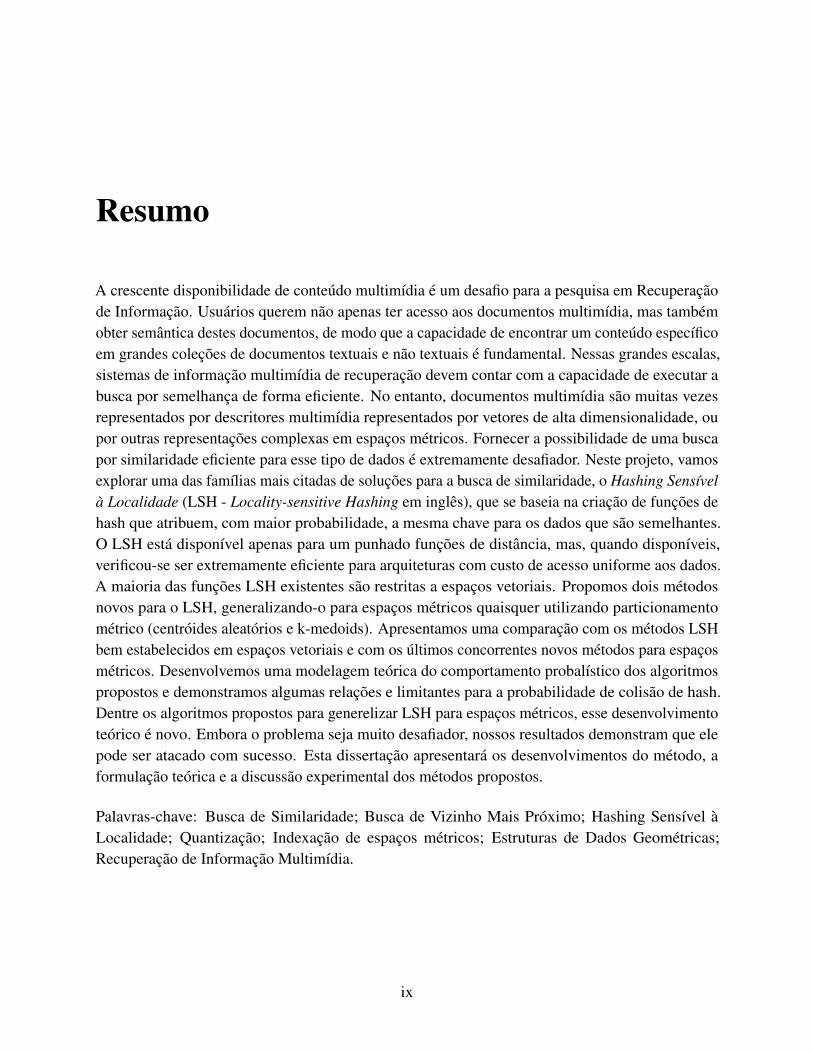
Resumo
A crescente disponibilidade de conteudo multimıdia e um desafio para a pesquisa em Recuperacaode Informacao. Usuarios querem nao apenas ter acesso aos documentos multimıdia, mas tambemobter semantica destes documentos, de modo que a capacidade de encontrar um conteudo especıficoem grandes colecoes de documentos textuais e nao textuais e fundamental. Nessas grandes escalas,sistemas de informacao multimıdia de recuperacao devem contar com a capacidade de executar abusca por semelhanca de forma eficiente. No entanto, documentos multimıdia sao muitas vezesrepresentados por descritores multimıdia representados por vetores de alta dimensionalidade, oupor outras representacoes complexas em espacos metricos. Fornecer a possibilidade de uma buscapor similaridade eficiente para esse tipo de dados e extremamente desafiador. Neste projeto, vamosexplorar uma das famılias mais citadas de solucoes para a busca de similaridade, o Hashing Sensıvela Localidade (LSH - Locality-sensitive Hashing em ingles), que se baseia na criacao de funcoes dehash que atribuem, com maior probabilidade, a mesma chave para os dados que sao semelhantes.O LSH esta disponıvel apenas para um punhado funcoes de distancia, mas, quando disponıveis,verificou-se ser extremamente eficiente para arquiteturas com custo de acesso uniforme aos dados.A maioria das funcoes LSH existentes sao restritas a espacos vetoriais. Propomos dois metodosnovos para o LSH, generalizando-o para espacos metricos quaisquer utilizando particionamentometrico (centroides aleatorios e k-medoids). Apresentamos uma comparacao com os metodos LSHbem estabelecidos em espacos vetoriais e com os ultimos concorrentes novos metodos para espacosmetricos. Desenvolvemos uma modelagem teorica do comportamento probalıstico dos algoritmospropostos e demonstramos algumas relacoes e limitantes para a probabilidade de colisao de hash.Dentre os algoritmos propostos para generelizar LSH para espacos metricos, esse desenvolvimentoteorico e novo. Embora o problema seja muito desafiador, nossos resultados demonstram que elepode ser atacado com sucesso. Esta dissertacao apresentara os desenvolvimentos do metodo, aformulacao teorica e a discussao experimental dos metodos propostos.
Palavras-chave: Busca de Similaridade; Busca de Vizinho Mais Proximo; Hashing Sensıvel aLocalidade; Quantizacao; Indexacao de espacos metricos; Estruturas de Dados Geometricas;Recuperacao de Informacao Multimıdia.
ix

x

Contents
Abstract vii
Resumo ix
Dedication xiii
Acknowledgements xv
1 Introduction 11.1 Defining the Problem . . . . . . . . . . . . . . . . . . . . . . . . . . . . . . . . . 21.2 Applications . . . . . . . . . . . . . . . . . . . . . . . . . . . . . . . . . . . . . . 21.3 Our Approach and Contributions . . . . . . . . . . . . . . . . . . . . . . . . . . . 3
1.3.1 Publications . . . . . . . . . . . . . . . . . . . . . . . . . . . . . . . . . . 4
2 Theoretical Background and Literature Review 52.1 Geometric Notions . . . . . . . . . . . . . . . . . . . . . . . . . . . . . . . . . . 5
2.1.1 Vector and Metric Space . . . . . . . . . . . . . . . . . . . . . . . . . . . 52.1.2 Distances . . . . . . . . . . . . . . . . . . . . . . . . . . . . . . . . . . . 72.1.3 Curse of Dimensionality . . . . . . . . . . . . . . . . . . . . . . . . . . . 82.1.4 Embeddings . . . . . . . . . . . . . . . . . . . . . . . . . . . . . . . . . 10
2.2 Indexing Metric Data . . . . . . . . . . . . . . . . . . . . . . . . . . . . . . . . . 102.3 Locality-Sensitive Hashing . . . . . . . . . . . . . . . . . . . . . . . . . . . . . . 13
2.3.1 Basic Method in Hamming Space . . . . . . . . . . . . . . . . . . . . . . 152.3.2 Extensions in Vector Spaces . . . . . . . . . . . . . . . . . . . . . . . . . 162.3.3 Structured or Unstructured Quantization? . . . . . . . . . . . . . . . . . . 182.3.4 Extensions in General Metric Spaces . . . . . . . . . . . . . . . . . . . . 18
2.4 Final Remarks . . . . . . . . . . . . . . . . . . . . . . . . . . . . . . . . . . . . . 19
3 Towards a Locality-Sensitive Hashing in General Metric Spaces 203.1 VoronoiLSH . . . . . . . . . . . . . . . . . . . . . . . . . . . . . . . . . . . . . . 20
3.1.1 Basic Intuition . . . . . . . . . . . . . . . . . . . . . . . . . . . . . . . . 203.1.2 Algorithms . . . . . . . . . . . . . . . . . . . . . . . . . . . . . . . . . . 223.1.3 Cost models and Complexity Aspects . . . . . . . . . . . . . . . . . . . . 24
xi

3.1.4 Hashing Probabilities Bounds . . . . . . . . . . . . . . . . . . . . . . . . 273.2 VoronoiPlex LSH . . . . . . . . . . . . . . . . . . . . . . . . . . . . . . . . . . . 31
3.2.1 Basic Intuition . . . . . . . . . . . . . . . . . . . . . . . . . . . . . . . . 323.2.2 Algorithms . . . . . . . . . . . . . . . . . . . . . . . . . . . . . . . . . . 333.2.3 Theoretical characterization . . . . . . . . . . . . . . . . . . . . . . . . . 34
3.3 Parallel VoronoiLSH . . . . . . . . . . . . . . . . . . . . . . . . . . . . . . . . . 353.4 Final remarks . . . . . . . . . . . . . . . . . . . . . . . . . . . . . . . . . . . . . 37
4 Experiments 384.1 Datasets . . . . . . . . . . . . . . . . . . . . . . . . . . . . . . . . . . . . . . . . 384.2 Techniques Evaluated . . . . . . . . . . . . . . . . . . . . . . . . . . . . . . . . . 394.3 Evaluation Metrics . . . . . . . . . . . . . . . . . . . . . . . . . . . . . . . . . . 404.4 Results . . . . . . . . . . . . . . . . . . . . . . . . . . . . . . . . . . . . . . . . . 41
4.4.1 APM Dataset: comparison with K-Means LSH . . . . . . . . . . . . . . . 424.4.2 Dictionary Dataset: Comparison of Voronoi LSH and BPI-LSH . . . . . . 454.4.3 Listeria Dataset: DFLSH and VoronoiPlex LSH . . . . . . . . . . . . . . . 474.4.4 BigANN Dataset: Large-Scale Distributed Voronoi LSH . . . . . . . . . . 49
5 Conclusion 515.1 Open questions and future work . . . . . . . . . . . . . . . . . . . . . . . . . . . 525.2 Concluding Remarks . . . . . . . . . . . . . . . . . . . . . . . . . . . . . . . . . 52
Bibliography 54
A Implementation 63
xii

In the memory of what we yet have to see
xiii

xiv

Acknowledgements
I would like to thank all the support I have received during this years of study. The support we needand receive are multivariate and changes over time and I must acknowledge that I would never comethis far without all the help and love and have received over these years.
I thank my supervisor, Prof. Dr. Eduardo Valle, for the patience, the trust and the lessons taughtabout a wide range of aspects in academic and professional life.
I thank and appreciate all the love my family has given me. Thank you dad (Jose), mom (Marta)and little brother (Elienai). Thank my love Juliana Vita. You have endured with me the hard timesand always given me encouragement to keep walking in the right track.
I thank this wide extended family of good friends and colleagues that I have around the world.A special thank to friends from Unicamp (specially people at APOGEEU, LCA, IEEE-CIS):Alan Godoy, David Kurka, Rafael Figueiredo, Raul Rosa, Paul Hidalgo, Micael Carvalho, CarlosAzevedo, Michel Fornacielli, Roberto Medeiros, Ricardo Righetto, and many others. I thank myfriends from ABU-Campinas, residents at Casa Douglas and visitors: Lois McKinney Douglas,Marcos Bacon, Jonas Kienitz, Tiago Bember, Carla Bueno, Esther Alves, Daniel Franzolin, PedroIvo, Maria (Maue), Edu Oliveira, Nathan Maciel, Micael Poget, Gabriel Dolara, Patrick Timmer,Paulo Castro, Fernanda Longo, and many others. I thank you all for the warm welcome in Campinas,for the friendly environment, the good and bad times spend together. It was really nice to sharesome of my time in Campinas with you all.
I thank the University of Campinas and the School of Electrical and Computer Engineeringfor being a high-level educational and research environment. A special thank to Prof. Dr. GeorgeTeodoro and Thiago Teixeira for the opportunity of excellent collaborative work. A special thank toCAPES for the financial support.
I thank God for guiding me and being the lenses through-with I see everything.
xv

xvi

List of Figures
1.1 Schematics of a CMIR system . . . . . . . . . . . . . . . . . . . . . . . . . . . . 3
2.1 Illustration of a hypothetical situation where the distance distribution gets moreconcentrated as the dimensionality increases and the filtered portion of the datasetusing a distance bound r0 ≤ d(p, q) ≤ r1 . If in a low dimensional space this boundimplied in searching over 10% of the dataset, in a higher dimensional space thisbound could lead to approximately 50% of the dataset being evaluated. . . . . . . . 9
2.2 Domination mechanism and range queries: which range queries can be answeredusing the upper and lower bounding distance functions? . . . . . . . . . . . . . . 11
2.3 LSH and (R, c)-NN: probability of reporting points inside closed ball BX(q, r) asR-Near of q is high. Probability of reporting points outside closed ball BX(q, cr)as cr-near neighbor of q is lower. Points in the middle may be wrongly reported asR-Near with some probability . . . . . . . . . . . . . . . . . . . . . . . . . . . . 14
2.4 E2LSH: projection on a random line and quantization . . . . . . . . . . . . . . . . 16
3.1 Each hash table of Voronoi LSH employs a hash function induced by a Voronoidiagram over the data space. Differences between the diagrams due to the datasample used and the initialization seeds employed allow for diversity among thehash functions. . . . . . . . . . . . . . . . . . . . . . . . . . . . . . . . . . . . . 21
3.2 Voronoi LSH: a toy example with points C = c1, c2, c3 as centroids, query pointp, relevant nearest neighbor q, irrelevant nearest neighbor p′, radii of search r andcr and random variables Zq, Zp and Zp′ . . . . . . . . . . . . . . . . . . . . . . . 27
3.3 Closed Balls centered at point q and p, illustrating the case where events withZq + Zp ≤ d(p, q), which implies that NNC(p) 6= NNc(q) . . . . . . . . . . . . . . 29
3.4 VoronoiPlex LSH: a toy example with points C = c1, c2, c3, c4, c5 as sharedcentroids between partitioning, choosing three centroids for each partitioning andconcatenating four partitioning in the final hash-value . . . . . . . . . . . . . . . . 32
4.1 (a) Listeria Gene Dataset string length distribution (b) English Dataset string lengthdistribution . . . . . . . . . . . . . . . . . . . . . . . . . . . . . . . . . . . . . . 39
4.2 APM Dataset: Comparison of VoronoiLSH with three centroids selections strategyK-means, K-medoids and Random for 10-NN . . . . . . . . . . . . . . . . . . . . 42
xvii

4.3 APM Dataset: Comparison of the impact of the number of cluster center in theextensivity metric and the correlation between extensivity and the recall for K-meansLSH, Voronoi LSH and DFLSH (10-NN) . . . . . . . . . . . . . . . . . . . . . . 43
4.4 Effect of the initialization procedure for the K-medoids clustering in the quality ofnearest-neighbors search . . . . . . . . . . . . . . . . . . . . . . . . . . . . . . . 45
4.5 Voronoi LSH recall–cost compromises are competitive with those of BPI (error barsare the imprecision of our interpretation of BPI original numbers). To make theresults commensurable, time is reported as a fraction of brute-force linear scan. . . 46
4.6 Different choices for the seeds of Voronoi LSH: K-medoids with different initial-izations (K-means++, Park & Jun, random), and using random seeds (DFLSH).Experiments on the English dictionary dataset. . . . . . . . . . . . . . . . . . . . . 46
4.7 Indexing time (ms) varying with the number of centroids. Experiments on theEnglish dictionary dataset. . . . . . . . . . . . . . . . . . . . . . . . . . . . . . . 47
4.8 Recall metric of VoronoiLSH using random centroids (DFLSH) for the Listeriagene dataset using L=2 and L=3 hash-tables and varying the number of centroids(obtaining varying extensivity) . . . . . . . . . . . . . . . . . . . . . . . . . . . . 48
4.9 Recall metric of VoronoiPlex LSH using random centroids (10 centroids selectedfrom a 4000 point sample set) for the Listeria gene dataset using L=1 and L=8hash-tables and varying the size w of the key-length . . . . . . . . . . . . . . . . 49
4.10 Random seeds vs. K-means++ centroids on Parallel Voronoi LSH (BigAnn). Well-chosen seeds have little effect on recall, but occasionally lower query times. . . . . 49
4.11 Efficiency of Parallel Voronoi LSH parallelization as the number of nodes usedand the reference dataset size increase proportionally. The results show that theparallelism scheme scales-up well even for a very large dataset, with modest overhead. 50
A.1 Class diagram of the system . . . . . . . . . . . . . . . . . . . . . . . . . . . . . 64
xviii

Chapter 1
Introduction
The success of the Internet and the popularization of personal digital multimedia devices (digitalcameras, mobile phones, etc.) has spurred the availability of online multimedia content. Meanwhile,the need to make sense from ever growing data collections has also increased. We face the challengeof processing very large collections, in many media (photos, videos, text and sound), geographicallydispersed, with assorted appearance and semantics, available instantaneously at the fingertips of theusers. Information Retrieval, Data Mining and Knowledge Management must attend to the needs ofthe “new wave” of multimedia data [Datta et al., 2008].
Scientific interest in Multimedia Information Retrieval has been steadily increasing, with theconvergence of various disciplines (Databases, Statistics, Computational Geometry, InformationSystems, Data Structures, etc.), and the appearance of a wide range of potential applications, forboth private and public sectors. As an example of this interest we refer to the Multimedia GrandChallenge1), opened in the ACM Multimedia conference of 2009, which consists of a competitionwith a set of problems and issues brought by the industry to the scientific community. Amongstothers, Datta et al. [2008] present results showing an exponential growth in the number of articlescontaining the keyword “Image Retrieval” as indicative of the growing interest in the area.
Similarity search is a key step in most of these systems (Information Retrieval, Machine Learningand Pattern Recognition Systems) and there is the need for supporting different distance functionsand data formats, as well as designing fast and scalable algorithms, specially for achieving thepossibility of processing billions or more multimedia items in a tractable time. The strategy forthis task may be twofold: improving data-structure and algorithms for sequential processing andadapting algorithms and data structure for parallel and distributed processing.
The idea of comparing the similarity of two (or more) abstract objects can be formally specifiedand intuitively comprehended using the concept of distance between points in some generic space.Thus, if we entertain the possibility of representing our abstract objects as points in some genericspace equipped with a distance measure, we may follow the intuition that the closer the distancebetween the points, the more similar the objects. This has been established as a standard theoreticaland applied framework in Content-based Multimedia Retrieval, Data Mining, Pattern Recognition,
1http://www.acmmm12.org/call-for-multimedia-grand-challenge-solutions/
1

1.1. Defining the Problem 2
Computer Vision and Machine Learning. Although such approach requires a certain level ofabstraction and approximation, it is very practical and appropriate for the task.
However, since there are many possible distance measures for different types of data (strings,text documents, image, video, sounds, etc.), solutions that are effective and efficient only for specificdistances measures are useful, but limited. Our purpose is to study existing specific solutions inorder to generalize them to generic metric space without loosing efficiency and effectiveness.
In this chapter we will define formally similarity search, discuss the available solutions andpresent its most common applications.
1.1 Defining the Problem
A definition of Metric Access Methods (MAM) is given by Skopal [2010]:
Set of algorithms and data structure(s) providing efficient (fast) similarity search underthe metric space model.
The metric space model assumes that the domain of the problem is captured by a metric spaceand that the measure of similarity between the objects of that domain can be represented using somedistance function in the metric space. Thus, the problem of finding, classifying or grouping similarobjects from a given domain is translated to a geometric problem of finding nearest-neighbor pointsin a metric space. The challenge is to provide data structures and algorithms that can accomplishthis task efficiently and effectively in a context of large scale search.
The obvious approach for the nearest neighbor search is a linear sequential algorithm that scanthe whole dataset. However this approach is not scalable in realistic set-ups with large datasetand large query sets. It would be an interesting result that using some refined data structure andalgorithm we achieve a much more efficient query performance.
Another challenge for the naive approach is the case of dataset with high-dimensionality,meaning, concentrated histogram of distances, sparsity of points and various other non-trivialphenomena related to high dimensionality. Exact algorithms has failed to tackle with this challengeand approximate methods has showed to be the most promising approach.
Finally we can enunciate our specific problem statement:
The development of effective and efficient methods (data structures and algorithms) forapproximate similarity search in generic metric space. The question is whether it wouldbe possible to offer better efficiency/effectiveness trade-off than available methods onthe literature and the condition that this improvement could be achieved.
1.2 Applications
Content-based multimedia information retrieval (CBMIR) is an alternative to keyword-based or tag-based retrieval, which works by extracting features based on distinctive properties of the multimedia
1.3. Our Approach and Contributions 3
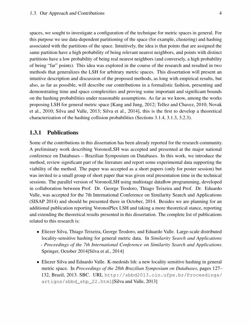
Multimedia DocumentsCollection Multimedia descriptors Store of descriptors
Query Query descriptors Most similar document
Search for stored descriptorsclose to query descriptor
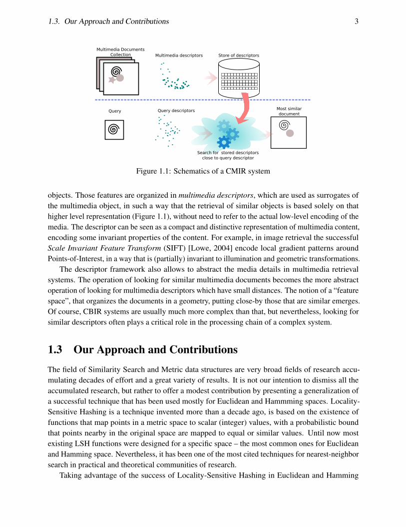
Figure 1.1: Schematics of a CMIR system
objects. Those features are organized in multimedia descriptors, which are used as surrogates ofthe multimedia object, in such a way that the retrieval of similar objects is based solely on thathigher level representation (Figure 1.1), without need to refer to the actual low-level encoding of themedia. The descriptor can be seen as a compact and distinctive representation of multimedia content,encoding some invariant properties of the content. For example, in image retrieval the successfulScale Invariant Feature Transform (SIFT) [Lowe, 2004] encode local gradient patterns aroundPoints-of-Interest, in a way that is (partially) invariant to illumination and geometric transformations.
The descriptor framework also allows to abstract the media details in multimedia retrievalsystems. The operation of looking for similar multimedia documents becomes the more abstractoperation of looking for multimedia descriptors which have small distances. The notion of a “featurespace”, that organizes the documents in a geometry, putting close-by those that are similar emerges.Of course, CBIR systems are usually much more complex than that, but nevertheless, looking forsimilar descriptors often plays a critical role in the processing chain of a complex system.
1.3 Our Approach and Contributions
The field of Similarity Search and Metric data structures are very broad fields of research accu-mulating decades of effort and a great variety of results. It is not our intention to dismiss all theaccumulated research, but rather to offer a modest contribution by presenting a generalization ofa successful technique that has been used mostly for Euclidean and Hammming spaces. Locality-Sensitive Hashing is a technique invented more than a decade ago, is based on the existence offunctions that map points in a metric space to scalar (integer) values, with a probabilistic boundthat points nearby in the original space are mapped to equal or similar values. Until now mostexisting LSH functions were designed for a specific space – the most common ones for Euclideanand Hamming space. Nevertheless, it has been one of the most cited techniques for nearest-neighborsearch in practical and theoretical communities of research.
Taking advantage of the success of Locality-Sensitive Hashing in Euclidean and Hamming
1.3. Our Approach and Contributions 4
spaces, we sought to investigate a configuration of the technique for metric spaces in general. Forthis purpose we use data-dependent partitioning of the space (for example, clustering) and hashingassociated with the partitions of the space. Intuitively, the idea is that points that are assigned thesame partition have a high probability of being relevant nearest neighbors, and points with distinctpartitions have a low probability of being real nearest neighbors (and conversely, a high probabilityof being “far” points). This idea was explored in the course of the research and resulted in twomethods that generalizes the LSH for arbitrary metric spaces. This dissertation will present anintuitive description and discussion of the proposed methods, as long with empirical results, butalso, as far as possible, will describe our contributions in a formalistic fashion, presenting anddemonstrating time and space complexities and proving some important and significant boundson the hashing probabilities under reasonable assumptions. As far as we know, among the worksproposing LSH for general metric space [Kang and Jung, 2012; Tellez and Chavez, 2010; Novaket al., 2010; Silva and Valle, 2013; Silva et al., 2014], this is the first to develop a theoreticalcharacterization of the hashing collision probabilities (Sections 3.1.4, 3.1.3, 3.2.3).
1.3.1 Publications
Some of the contributions in this dissertation has been already reported for the research community.A preliminary work describing VoronoiLSH was accepted and presented at the major nationalconference on Databases – Brazilian Symposium on Databases. In this work, we introduce themethod, review significant part of the literature and report some experimental data supporting theviability of the method. The paper was accepted as a short papers (only for poster session) butwas invited to a small group of short paper that was given oral presentation time in the technicalsessions. The parallel version of VoronoiLSH using multistage dataflow programming, developedin collaboration between Prof. Dr. George Teodoro, Thiago Teixeira and Prof. Dr. EduardoValle, was accepted for the 7th International Conference on Similarity Search and Applications(SISAP 2014) and should be presented there in October, 2014. Besides we are planning for anadditional publication reporting VoronoiPlex LSH and taking a more theoretical stance, reportingand extending the theoretical results presented in this dissertation. The complete list of publicationsrelated to this research is:
• Eliezer Silva, Thiago Teixeira, George Teodoro, and Eduardo Valle. Large-scale distributedlocality-sensitive hashing for general metric data. In Similarity Search and Applications- Proceedings of the 7th International Conference on Similarity Search and Applications.Springer, October 2014[Silva et al., 2014]
• Eliezer Silva and Eduardo Valle. K-medoids lsh: a new locality sensitive hashing in generalmetric space. In Proceedings of the 28th Brazilian Symposium on Databases, pages 127–132, Brazil, 2013. SBC. URL http://sbbd2013.cin.ufpe.br/Proceedings/
artigos/sbbd_shp_22.html[Silva and Valle, 2013]
Chapter 2
Theoretical Background and LiteratureReview
In this chapter we will present and discuss extensively the concepts necessary to understand ourcontributions and the state-of-art on the subject. At first, we will introduce the basic mathematicaland algorithmic notions and notations. In the sequence, we will discuss how the broader problemof Similarity Search in Metric Spaces has been approached in the specialized literature, howevernot diving deeply in each specific method references. We will focus the discussion on the mainideas applied to metric indexing and refer the reader to detailed surveys of the algorithms. Further,Locality-Sensitive Hashing is addressed and discussed in details, including a formal presentation ofthe algorithms and a mathematical demonstrations of selected properties.
2.1 Geometric Notions
In this dissertation we will use the framework of Metric Space to address the problem of SimilaritySearch. We adopt this model because of it generality and versatility. Any collection of objectsequipped with a function measuring the similarity of the objects and obeying a small sets of axioms(the metric axioms) are enabled to be analyzed and processed using the tools developed for metricspaces.
Another advantage is the possibility of using geometric reasoning and intuition in the analysisof objects that are not trivially thought as geometric (for example, strings, or text documents). So,in this setting, it is possible to speak of a “ball” around a string using Edit distances, for example.In this section we will develop some of these intuitions, formalizing geometric notions as balls andtriangular inequality over generic metric space.
2.1.1 Vector and Metric Space
We will briefly present the definition and axioms of metric space and the fundamental operationswe are interested in metric spaces.
5

2.1. Geometric Notions 6
Metric space are general sets equipped with a metric (or distance), which is a real-valuedpositive function between pairs of points. Given that we have a definition of sets of objects and adefinition of a function comparing pairs of objects (obeying certain properties), we have a metricspace. The distance function must obey basically four axioms: the image of the distance function ofnon-negative, the function is symmetric in relation to the order of the points, points with distancezero are equals, and the triangle inequality.
Definition 2.1 (Metric space properties). Metric space: given a set U (domain) and a functiond : U × U → R (distance or dissimilarity function), a pair (U, d) is a metric space if the distancefunction d have the following properties [Chavez et al., 2001]:
• ∀x, y ∈ U , d(x, y) ≥ 0 (non-negativeness)
• ∀x, y ∈ U , d(x, y) = d(y, x) (symmetry)
• ∀x, y ∈ U , d(x, y) = 0⇔ x = y (identity of indiscernibles)
• ∀x, y, z ∈ U , d(x, y) ≤ d(x, z) + d(z, y) (triangle inequality)
If we want to build a notion of neighborhood for points in metric space there is only one tool touse: the distance information between pairs of points. A natural way of accomplish that is to definea distance range around of a point and analyze the region of the space in that range; this idea issimilar to looking to an interval with a central point in the real line, using distance between points,generalized to metric space. This definition is useful for a set of indexing method that partition thespace using metric balls.
Definition 2.2 (Open and Closed ball). Given a set X in a metric space (U ,d) and a point p ∈ Xwe define the Open Ball of radius r around p as the set BX(p, r) = x|d(x, p) < r, x ∈ X and theClosed Ball of radius r around p as BX [p, r] = x|d(x, p) ≤ r, x ∈ X.
Definition 2.3 (Finite Vector Spaces). A given metric space (U, d) is a finite-dimensional vectorspace (which for the sake of briefness we will refer simply as a vector space) with dimension D ifeach x ∈ U can be represented as a tuple of D real values, x = (x1, . . . , xD). The most commondistance for vector space are the Lp distances [Chavez et al., 2001; Skopal, 2010].
• ∀x, y ∈ U , where x = (x1, . . . , xD) and y = (y1, . . . , yD),Lp(x, y) = p
√∑Di=1 |xi − yi|p
Now we define three fundamental search problems central for similarity search in metric spaces:Range Search, K-Nearest Neighbor Search and (R, c)-Nearest Neighbor Search. Given a subset ofmetric space and a subset of queries, the Range Search problem is of finding efficiently a metricball of data points around query points given radius as parameter (called range).
Definition 2.4 (Range search). Given the metric space (U, d), a dataset X ⊂ U , a query pointq ∈ U and a range r, find the set R(q, r) = x ∈ X|d(q, x) ≤ r [Clarkson, 2006].

2.1. Geometric Notions 7
Definition 2.5 (K-Nearest Neighbors (kNN) search). Given the metric space (U, d), a datasetX ⊂ U , a query point q ∈ U and an integer k, find the set NNX(q, k), defined as |NNX(q, k)| =k and (∀x ∈ X\NNX(q, k))(∀y ∈ NNX(q, k)) : d(y, q) ≥ d(x, q) (the k closest points toq) [Clarkson, 2006].
A related problem is the (c, R)-Nearest Neighbor, defined as the approximate nearest neighborfor a given radium.
Definition 2.6 (c-approximate R-near neighbor, or (c, R)-NN [Andoni and Indyk, 2006]).Given a set X of points in a metric space (U, d) , and parameters R > 0, δ > 0, construct adata structure such that, given any query point q ∈ U , if there is p ∈ X with d(p, q) ≤ R (p is aR-near point of q), it reports some point p∗ ∈ X with d(p∗, q) ≤ cR (p∗ is a cR-near neighbor of qin X) with probability at least 1− δ.
Given many challenges for large scale search in metric spaces, the choice for approximateand random algorithms is justified because of the possibility of quality/time (efficiency/efficacy)trade-off which may be favorable for a scaling of the algorithms under acceptable error rates.Patella and Ciaccia [2009] presents a survey of approximate methods and the major challenges ofapproximate search in spatial (vector) and metric data.
2.1.2 Distances
There are a variety of possible distance definitions over a variety of objects. We will restrainourselves to present just a small sample of the population of metric distances. Our aim is just toillustrate and contextualize our discussion of Similarity Search presenting some distances that areuseful in applications, specially in Content-Based Multimedia Retrieval, Machine Learning, PatternRecognition, Databases and Data Mining.
The usual distances functions in coordinate spaces (in special Euclidean) are Lp distance, knownalso as Minkowski distance. Lp distances are related to our most elementary geometric intuitionsand are widely applied in models of similarity and distance-based algorithms; for example, Skopal[2010] says that more than 80% of relevant literature in metric indexing apply Lp distances.
Definition 2.7 (Lp distances on finite dimensional coordinate spaces). Given a coordinate metricspace (U, d), of dimensionality D, the Lp distance of two points p = (p1, · · · , pD),q = (q1, · · · , qD)is defined as
Lp(p, q) =(
D∑i=1|pi − qi|p
)1/p
Euclidean metric space with D dimensions equipped with a Lp metric may be referred as LDpspace.
Three Lp distances with widespread use are the Euclidean (p = 2), Manhattan (p = 1, alsoknown as Taxicab metric), and the Chebyshev (p =∞, also known as the maximum metric). The

2.1. Geometric Notions 8
Euclidean distance is related with common analytic geometry, and is the generalization for higherdimensions of the Pythagorean distance of two points in the plane – the square root of a sum ofsquares.
Another import definition is the distance from a point to a set, a composite of distance toindividual points in the set. This concept will be applied in the analysis of our proposed methods
Definition 2.8 (Point distance to sets). Given a metric space (U, d), a point x ∈ U and set C ⊆ U ,d(x,C) is defined as the distance from x to the nearest point in C.
• d(x,C) = mind(x, c)|c ∈ C
These are restricted examples of a long and diverse set of distances; we choose to define hereonly the ones that are necessary for the understanding of concepts and algorithms described in thisdissertation. Deza and Deza [2009] has done a compendious work of cataloging an exhaustivecollection of distance and metric; that is proper reference for the reader interested in further detailsand more examples of distances and metric.
2.1.3 Curse of Dimensionality
The “Curse of Dimensionality” (CoD) is a generic term associated with intractability and challengeswith growing dimensionality of the search space in algorithms for statistical analysis, mathematicaloptimization, geometric operations and other areas. It is related to the fact that the geometricintuition in lower dimensionality sometimes are totally changed in higher dimensionality, and manytimes in a way that undermines the strategies that worked in lower dimensions. However not allproperties associated with the curse are always negative: depending on the subject area the cursecan be a blessing [Donoho et al., 2000]. It was first coined by Bellman [1961] as an argumentagainst the strategy that use a discretization and a brute force over the search space, in the contextof optimization and dynamic programming. The argument is simple: the number of partition growsexponentially with the dimensionality, meaning, to approximately optimize of function over a spacewith dimensionality D using grid search, to achieve a error ε we would need search over (1/ε)Dgrids [Donoho et al., 2000].
In Similarity Search (Metric Access Methods and Spatial Access Methods) the curse has beenrelated to the difficulty to prune the search space as the (intrinsic) dimensionality grows – theperformance of many methods in high-dimensions are no better than linear scan. Also the verynotion of nearest-neighbor in high-dimensional space becomes blurred, specially when the distanceto the nearest point and the distance to the farthest point in the dataset becomes indistinguishable: ithas been demonstrated general conditions over the distance distribution, covering a wide class ofdata and query workload, implying with high probability that as the dimensionality increases thedistance to farthest point and to the closest point are practically the same [Aggarwal et al., 2001;Shaft and Ramakrishnan, 2006; Beyer et al., 1999]. This effect has been related to concentration ofdistance and the intrinsic dimensionality of the dataset [Chavez et al., 2001; Shaft and Ramakrishnan,2006; Pestov, 2000, 2008], but it is still an open question what is the formulation that explains how

2.1. Geometric Notions 9
- 3 - 2 - 1
0.8
0.6
0.4
0.2
0.0
−5 −3 1 3 5x
1.0
−1 0 2 4−2−4
pdf(x)
[r0,r1]
Figure 2.1: Illustration of a hypothetical situation where the distance distribution gets more concen-trated as the dimensionality increases and the filtered portion of the dataset using a distance boundr0 ≤ d(p, q) ≤ r1 . If in a low dimensional space this bound implied in searching over 10% of thedataset, in a higher dimensional space this bound could lead to approximately 50% of the datasetbeing evaluated.
the difficulties for similarity search emerges. In fact Volnyansky and Pestov [2009] demonstratesthat, under several general workloads and appropriate assumptions, pivot-based methods presentsconcentration of measure using the fact that these methods can be seen as a 1-Lipschitz embedding(the mapping to pivot space) and this can degenerate the performance of a large class of metricindexing methods. Intuitively is possible to see that if we are using bounds on the distancedistribution to perform a fast similarity search, a sharp concentrated distribution can be much moredifficult to search: as the distribution get concentrated around some value, a larger portion of thedataset is not going to be filtered by the bounds – in the limit we would have a full scan of thedataset. If in a low dimensional space, a distance bound [r0, r1] (r0 ≤ d(p, q) ≤ r1) can be appliedto filter out a huge portion of the dataset, in a higher space with concentrated distance distribution,this same bound could filter out very few points; in order to achieve an equivalent selectivity, wewould need a more sharper bound, a process that could lead to very unstable query processing,where a small numerical perturbation on the distances would imply large performance loss (seeFigure 2.1 for a illustration).
Recently the hubness phenomenon has been studied and associated with high-dimensionalityand the CoD. Hubs are points that consistently appear in the kNN set of many other points in thedataset. Although hubness and concentration of measure are distinct phenomena, both emergeswith increasing dimensionality. However, this property can also be exploited positively to avoidproblem of high-dimensionality. In fact, if there is natural clusters in the dataset, and the hubnessproperty holds, it is expected that with increasing dimensionality the clusters become more well-defined [Radovanovic et al., 2009, 2010], in this situation metrics based on shared nearest-neighborscan offer good potential results [Flexer and Schnitzer, 2013].
2.2. Indexing Metric Data 10
2.1.4 Embeddings
Since there is long standing solutions for proximity search in more specific space (for exampleEuclidean or Vector spaces), a possible general approach to the problem is the mapping from generalmetric space to those space where a solution already exists – a general technique in ComputerScience, reduction of an unsolved problem to another problem with a known solution. In order forthose mappings to be useful, some properties of the original space must be preserved, specificallythe distance information for any pairs of points in the original space. There are also techniquesfocusing on preserving volume (or content) information between spaces [Rao, 1999], but we willnot discuss them.
Our theoretical and practical interest for approximate similarity search relies over a class ofembedding that preserve distances between pairs to a certain degree of distortion from the originaldistance. In special we are interested in Lipschitz embedding with a fixed maximum distortion.
Definition 2.9 (c-Lipschitz mapping [Deza and Deza, 2009]). Given a positive scalar c, a c-Lipschitzmapping is a mapping f : U → S such that dS(f(p), f(q)) ≤ cd(p, q), for p, q ∈ U .
Definition 2.10 (Bi-Lipschitz mapping [Deza and Deza, 2009]). Given a positive scalar c, metricspaces (U, dU) and (S, dS), a funtion f : U → S is a c-bi-Lipschitz mapping if exists a scalar c > 0such that: 1/cdU(p, q) ≤ dS(f(p), f(q)) ≤ cdU(p, q), for p, q ∈ U .
A simple example of 1-Lipschitz embedding is the pivot-space (as we will see later, this is thebasis for a whole family of metric indexing methods): given metric space (M,d), take k points asthe pivot set P = p1, · · · , pk, and build the mapping gP (x) = (d(x, p1), · · · , d(x, pk)). Calcu-lating the maximum metric over two embedded points x, y ∈ M we obtain L∞(gP (x), gP (y)) =maxi∈1,···k|d(x, pi)−d(y, pi)| and by triangle inequality |d(x, pi)−d(y, pi)| ≤ d(x, y),∀pi ∈M 1.
In general there are results indicating that an n−points metric can be embedded in Euclideanspace with log(n) distortion [Matousek, 1996; Bourgain, 1985; Matousek, 2002]. The readerinterested in further details about metric space embeddings should refer to the works of Deza andLaurent [1997] and Matousek [2002].
By relying on the general theory of embedding, one can advance the theoretical and practicalunderstanding of a great number of similarity search algorithms in metric space. Although notalways explicitly stated, many times embeddings are essential components of those algorithms. Inthe next section we will discuss how this is accomplished in some classes of algorithms.
2.2 Indexing Metric Data
The basic purpose of indexing metric data is to avoid a full sequential search, decreasing thenumber of distance computations and points processed. We may think of it as a data structurepartitioning the data space in such a way that the query processing is computationally efficient and
1d(x, y) + d(y, pi) ≥ d(x, pi) ⇒ d(x, y) ≥ d(x, pi) − d(y, pi) and d(x, y) + d(x, pi) ≥ d(y, pi) ⇒ d(x, y) ≥d(y, pi)− d(x, pi), meaning that |d(y, pi)− d(x, pi)| ≤ d(x, y)

2.2. Indexing Metric Data 11
qdL(q,x)
dU(q,x)
Yes
No
Maybe
d(q,x)<R?
Figure 2.2: Domination mechanism and range queries: which range queries can be answered usingthe upper and lower bounding distance functions?
effective. Even if we increase the amount of pre-processing, in the long run, in a scenario withmultiples queries arriving, the whole process is much more efficient than sequential search. So agood indexing structure should display a polynomial complexity in the pre-processing phase and asub-linear complexity in the query search phase. We may also understand the index structure as theimplementation of some sort of metric filtering strategy.
Hetland [2009], in a more recent survey of metric indexing methods, tries to uncover themost essential principles and mechanisms from the vast literature of metric methods, synthesizingprevious surveys and reference work on metric indexing [Chavez et al., 2001; Hjaltason and Samet,2003; Zezula et al., 2006]. Leaving aside detailed algorithm description and thorough literaturediscussion, the author focus on the metric properties, distance bounds and index constructionmechanisms constituting the building blocks of widespread metric indexing methods. In general,before taking into account specific metric properties, the author highlights three mechanisms fordistance index construction: domination, signature and aggregation. Domination is the adoptionof computationally cheaper distances, lower and upper bound of the original distance, in orderto avoid distance calculation (if the distance function dU is always greater or equal to anotherdistance d, than dU dominates d). Applying domination mechanisms to range queries is usefulfor avoiding expensive distance computation. For example, given two distance function boundingthe original distance such that for any pairs of points p and q, dL(p, q) ≤ d(p, q) ≤ dU(p, q), ifrange R is greater than dU(p, q) the query “d(p, q) < R?” can be positively answered without thecalculation of d(p, q). Symmetrically, distance computation can be avoided when range R is lessthan dL(p, q) ( Figure 2.2 illustrates both situation). For instance, if distance functions dL and dU iscomputationally cheaper than distance d, we obtain a mechanism for improving the index efficient.Another lower bounding mechanism is a mapping that take points from the original space to asignature space. The signature of a point is a new representation of the object in distinct spacesuch that the distance computed using the signature is a lower bound to the distance in the original

2.2. Indexing Metric Data 12
space. Take two points p and q in the original space U , a non-expansive mapping (also known as1-Lipschitz mapping, Definition 2.9) is a function from the original space U to the signature space S,σ : U → S, such that dS(σ(p), σ(q)) ≤ d(p, q); a non-expensive mapping is an example of lowerbound in the signature space. It is possible to see that any Lipschitz or Bi-Lipschitz (Definition 2.10)mapping could be used as a signature mapping. The aggregation mechanism, used more often inconjunction with signature or dominance mechanism, consists in partitioning the search space inregions such that the distance bounds are applied on the aggregate rather than in individual pointsof the dataset. Those principles are used in specific metric mechanism for indexing:
• Pivoting and Pivot Scheme: a selected set of points P = p1, · · · , pk and the dataset isstored with precomputed distance information that later is used to lower-bound the distancefrom queries to points in the dataset. Given a point q in the dataset, a query q and the pivot set,there is a lower-bound to the query to points in the dataset given by maxi∈1,···k|d(p, pi)−d(q, pi)| ≤ d(p, q).
• Metric balls and shells: pivot and search spaces are organized in ball and shell partitions inorder to avoid distances calculations (aggregation). Generally some information regardingthe radius of the aggregate region must be stored with the index in order to apply metricdistance bound using a representative point of the region, but taking into consideration all theother points. Most metric tree methods apply this technique, but also methods like List-of-Clusters (a hierarchical list of metric balls inside metric shells) [Chavez and Navarro, 2005;Fredriksson, 2007].
• Metric Hyperplanes and Dirichlet Domains: in this case the regions are not of a particularshape, but are the result of dividing the metric dataset using metric hyperplanes. Taking twopoint p1 and p2, we can divide the space using the distance to these points; points closer to p1
form a region, and points closer to p2 is another region – the separating metric hyperplaneis the set of points with d(x, p1) = d(x, p2). This idea can be generalized if we use manyreference points, or hierarchical organization of the partitions. Chavez et al. [2001] use thecompact partition relation to analyze different techniques relying on metric hyperplanes.
The survey by Chavez et al. [2001], despite being dated and not covering a considerable numberof new relevant techniques, is still very relevant since many challenges for similarity search are stillnot solved and open to new methods and approaches. However, Chavez et al. [2001] shows thatthose different views of metric indexing are equivalent and can be comprehensively understoodusing the unifying model of equivalent relations, equivalent classes and partitioning. This unifiedmodel is applied to the development of a rigorous algorithmic analysis of metric indexing methods,specifically methods based on pivot-spaces and metric hyperplanes (denominated compact partitionsalso), where lower-bound on the probability of discarding whole partition classes are given and arerelated to a specific measure of intrinsic dimensionality (square of the mean over the square of thevariance of the distance histogram).
2.3. Locality-Sensitive Hashing 13
Metric trees: Burkhard and Keller [1973] (BK-Tree), in their seminal work, introduced a treestructure for searching with discrete metric distances. More recently, Uhlmann [1991] introducedthe concept of a “metric tree”, which can be seen as a generalization of the BK-Tree for generalmetric distances. The Vantage-Point Tree (VPT), by Yianilos [1993] is a binary metric tree thatstarts with a random root point, and then separates the dataset into left and right subtrees usingthe median distance as separating criterion. The M-tree [Ciaccia et al., 1997] is a balanced treeconstructed using only distance information: at search phase, it used the triangle-inequality propertyto prune the nodes to be visited. Slim-tree [Traina et al., 2000, 2002] is a dynamic metric tree withenhanced feature including the minimizing the overlap between nodes of the metric tree using aMinimum Spanning Tree algorithm.
Permutation-based Indexing: a recent family of MAM is the permutation-based indexing meth-ods. This methods are based on the idea of taking a reference set (permutants), and using theperspective of any point to the permutants, the distance ordering from a point in the dataset to thepermutants, as a relevant information for approximate search [Chavez et al., 2005; Gonzalez et al.,2008; Amato and Savino, 2008]. This ordering is very interesting because it is mapping from ageneral metric space to a permutation space, which a potentially cheaper distance function that canbe exploited to render new bound and offer better performance. In fact, this mapping can be usedwith a inverted-file and compared using Spearman Rho, Kendall Tau or Spearman Footrule measureto perform approximate search in an effective procedure [Gonzalez et al., 2008; Amato and Savino,2008].
For a comprehensive survey of Metric Access Methods the reader may refer to existing sur-veys [Chavez et al., 2001; Hjaltason and Samet, 2003; Zezula et al., 2006; Samet, 2005; Hetland,2009; Clarkson, 2006]. Skopal [2010] and Zezula [2012] offer a critical review of the evolution ofthe area, and an evaluation of possible future directions, making explicit claims about the necessityof even more scalable algorithms for the future of the area. The PhD thesis of Batko [2006] is alsoa good recent reference and survey for Metric Access Methods and general principles of metricindexing.
2.3 Locality-Sensitive Hashing
The LSH indexing method relies on a family of locality-sensitive hashing function H [Indyk andMotwani, 1998] to map objects from a metric domain X in a D-dimensional space (usually Rd)to a countable set C (usually Z), with the following property: nearby points in the metric spaceare hashed to the same value with high probability. It is presented in the seminal article [Indykand Motwani, 1998] as an efficient and theoretically interesting approach to the ApproximateNearest-Neighbors problem and later also as a solution for the (R, c)-NN problem [Datar et al.,2004; Andoni and Indyk, 2006] (Figure 2.3). A parallel line of work by Broder et al. [2000]developed the idea of MinHash (Min-Wise Independent Permutations) for fast estimation of set anddocuments similarity and later SimHash [Charikar, 2002] for cosine distance in vectors, using a

2.3. Locality-Sensitive Hashing 14
qr
crp
p'
Figure 2.3: LSH and (R, c)-NN: probability of reporting points inside closed ball BX(q, r) as R-Near of q is high. Probability of reporting points outside closed ball BX(q, cr) as cr-near neighborof q is lower. Points in the middle may be wrongly reported as R-Near with some probability
(slightly) distinct formulation of LSH. However, both formulations relied on a definition that relatedsimilarities (and distances) between objects and hash probabilities. We will follow the formulationof Indyk and Motwani [1998]2.
Definition 2.11. Given a distance function d : X×X → R+, a function family H = h : X → Cis (r, cr, p1, p2)-sensitive for a given data set S ⊆ X if, for any points p, q ∈ S, h ∈ H:
• If d(p, q) ≤ r then PrH [h(q) = h(p)] ≥ p1 (probability of colliding within the ball of radiusr),
• If d(p, q) > cr then PrH [h(q) = h(p)] ≤ p2 (probability of colliding outside the ball ofradius cr)
• c > 1 and p1 > p2
A function family G is constructed by concatenating M randomly sampled functions hi ∈ H ,such that each gj ∈ G has the following form: gj(v) = (h1(v), ..., hM(v)). The use of multiple hi
2It is worth noting that the authors of these articles, Andrei Broder, Moses Charikar and Piotr Indyk, werenamed recipients of the prestigious Paris Kanellakis Theory And Practice Award in 2012 for their contribution in thedevelopment of LSH. ACM Awards Page: The Paris Kanellakis Theory and Practice Award, http://awards.acm.org/kanellakis/, acessed in June, 7, 2014.

2.3. Locality-Sensitive Hashing 15
functions reduces the probability of false positives, since two objects will have the same key for gjonly if their value coincide for all hi component functions. Each object v from the input dataset isindexed by hashing it against L hash functions g1, . . . , gL. At the search phase a query object q ishashed using the same L hash functions and the objects stored in the given buckets are used as thecandidate set. Then, a ranking is performed among the candidate set according to their distance tothe query, and the k closest objects are returned.
LSH works by boosting the locality sensitiveness of the hash functions. As M grows, theprobability of a false positive (points that are far away having the same value on a given gj) dropssharply, but so grows the probability of a false negative (points that are close having differentvalues). But as L grows and we check all hash tables, the probability of false negatives falls, and theprobability of false positives grows. LSH theory shows that it is possible to set M and L so to havea small probability of false negatives, with an acceptable number of false positives. This allows thecorrect points to be found among a small number of candidates, dramatically reducing the numberof distance computations needed to answer the queries.
The need to maintain and query L independent hash tables is the main weak point of LSH. Inthe effort to keep both false positives and false negatives low, there is an “arms race” between Mand L, and the technique tends to favor large values for those parameters. The large number ofhash tables results in excessive storage overheads. Referential locality also suffers, due to the needto random-access a bucket in each of the large number of tables. More importantly, it becomesunfeasible to replicate the data on so many tables, so each table has to store only pointers to thedata. Once the index retrieves a bucket of pointers on one hash table, a cascade of random accessesensues to retrieve the actual data.
2.3.1 Basic Method in Hamming Space
The basic scheme [Indyk and Motwani, 1998] (Hamming LSH) provided locality-sensitive familiesfor the Hamming distance on Hamming spaces, and the Jacquard distance in spaces of sets.
The original [Indyk and Motwani, 1998] method is limited to Hamming space (bit-vectors offixed size) using Hamming distance (dH , which is the number of different bits at corresponding po-sitions, a sum of exclusive-or operation) and point-set space using Jaccard similarities. Equation 2.1describes the hash functions family for Hamming distance. The idea is to choose one position of thehamming point coordinate as representative of the point.
H = hi : 0, 1D → 0, 1 ∈ Zhi((b1, · · · , bD)) = bi, 1 ≤ i ≤ D
(2.1)
Because the distance between two hamming points is bounded and the number of different hashingfunction also is bounded, it is easy to see that the probabilities p1 and p2 are bounded and obeyingthe restriction of the LSH definition. Indeed, there are D possible functions hi for a given Hammingspace of dimensionality D and the hamming distance between two points measures the number oftimes (over the D possible) that the hashing of the two points are supposed to have distinct values.
2.3. Locality-Sensitive Hashing 16
Figure 2.4: E2LSH: projection on a random line and quantization
Thus, the probability of not colliding is given by:
Phi∼H [hi(q) 6= hi(p)] = dH(q, p)|H|
= dH(p, q)D
Considering the case of dH(q, p) > cr, we obtain
Phi∼H [hi(q) 6= hi(p)] = dH(p, q)D
>cr
D
⇒ Phi∼H [hi(q) = hi(p)] = 1− Phi∼H [hi(q) 6= hi(p)] < 1− cr
D
And if dH(q, p) ≤ r,Phi∼H [hi(q) 6= hi(p)] ≤
r
D
⇒ Phi∼H [hi(q) = hi(p)] ≥ 1− r
D
So it is clear that H is a (r, cr, 1− rD, 1− cr
D)-sensitive hashing function for Hamming metric
space.
2.3.2 Extensions in Vector Spaces
For several years those were the only families available, although extensions for L1-normed(Manhattan) and L2-normed (Euclidean) spaces were proposed by embedding those spaces intoHamming spaces [Gionis et al., 1999].
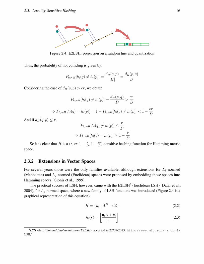
The practical success of LSH, however, came with the E2LSH3 (Euclidean LSH) [Datar et al.,2004], for Lp-normed space, where a new family of LSH functions was introduced (Figure 2.4 is agraphical representation of this equation):
H = hi : RD → Z (2.2)
hi(v) =⌊
ai.v + biw
⌋(2.3)
3LSH Algorithm and Implementation (E2LSH), accessed in 22/09/2013. http://www.mit.edu/˜andoni/LSH/

2.3. Locality-Sensitive Hashing 17
ai ∈ RD is a random vector with each coordinate picked independently from a Gaussiandistribution N(0, 1), bi is an offset value sampled from uniform distribution in the range [0, . . . , w]and w is a fixed scalar that determines quantization width. Applying hi to a point or object vcorresponds to the composition of a projection to a random line and a quantization operation, givenby the quantization width w and the floor operation.
Andoni and Indyk [2006] extends LSH using geometric ball hashing and lattices. This approachachieves a complexity near the lower bound established by Motwani et al. [2006] and O’Donnellet al. [2014] for LSH-based algorithms. Instead of projecting the high-dimensional points to aline, as in Datar et al. [2004] and Indyk and Motwani [1998], it is done a projection to a lower-dimensional space with dimension k D greater than one (D is the original space dimension) and“ball partitioning” quantization on the low-dimensional space. Nevertheless, for practical purposes(fast encoding and decoding) Leech lattices quantizer is used as alternative to “ball partitioning”quantizer. The Leech lattice is a dense lattice in the 24-dimensional space introduced by Leech[1964] for the problem of ball packing.
Query adaptive LSH [Jegou et al., 2008] introduces a dynamic bucket filtering scheme basedon the relative position of the hashed (but not quantized) value of the query point to the quantizercell frontier. Suppose the hashing function h(x) may be seen as the composition of a functionf : M → R, mapping the point to a scalar value, and a quantizer g : x→ bxc. The cell frontier ofh(x) is bf(x)c and bf(x)c+ 1, and distance to the center of the cell given by |bf(x)c− f(x) + 1/2|can be seen as a relevance criterion for the quality of the bucket. The further from the cell frontier(or closer to the cell center), the better the quality of the bucket. Using this as a relevance criteria,the “best” buckets are selected without using any point-wise distance calculation.
Panigrahy [2006] proposes entropy based LSH, an alternative approach to LSH in high-dimensional nearest neighbor search that employs very few hash tables (often just one), andfor the search phase, probes multiple randomly “perturbed” buckets around the query bucket in eachtable, in order to maintain the probabilistic response guarantees. Theoretical analysis support theassertion that this approach renders similar performance to the basic LSH. Although the numberof probes is very large, increasing the query costs, the trade-off might still be interesting for someapplications, specially in very large-scale databases, since main memory might be a system-wideconstraint, while processing time might be available.
Multiprobe LSH [Lv et al., 2007] follows the approach of Panigrahy, that, instead of using theexpensive random probes, generates a carefully probing sequence, visiting first the buckets mostlikely to contain the results. The probing sequence follows a success likelihood estimation, whichgenerates an optimal probing sequence, whose quality can be controlled by setting the number ofprobes. Joly and Buisson’s a posteriori multi-probe LSH [Joly and Buisson, 2008] extends thatwork by turning the likelihoods into probabilities by incorporating a Gaussian prior estimated fromtraining data, into a scheme aptly called a posteriori LSH. They employ an “estimated accuracyprobability” stop criterion instead of a number of probes.
Other contributions approach the problem of parameter tuning and the dynamic adaptation of theLSH method. LSH Forest [Bawa et al., 2005] uses variable-length hashes and a prefix-tree structurefor self-tuning of the LSH parameters. Ocsa and Sousa [2010] propose a similar adaptive multilevel

2.3. Locality-Sensitive Hashing 18
LSH index for dynamic index construction, changing the hash length parameter in each level of thestructure. A more recent work by Slaney et al. [2012] focus on the optimization of the parametersusing prior knowledge of the distance distribution of the base to achieve a desired quality level ofthe nearest neighbor method.
2.3.3 Structured or Unstructured Quantization?
In original LSH formulation [Indyk and Motwani, 1998; Gionis et al., 1999; Datar et al., 2004;Andoni and Indyk, 2006], the hashing schemes are based on structured random quantization of thedata space and this regularity is useful for the bounds on the hash collision probability. However,the question could be raised whether this structure is really necessary for locality-sensitiveness andif other non-regular partitioning could be applied. This discussion concerns how distinct space ordata partitioning be useful in the LSH framework.
Indeed, early proposals, Hamming LSH and E2LSH for example, used exclusively regularquantizers of the space independent with the data. However, K-means LSH [Pauleve et al., 2010]presents a comparison between structured (random projections, lattice) and unstructured (K-meansand hierarchical K-means) quantizers in the task of searching high dimensional SIFT descriptors,resulting on the proposal of a new LSH family based on the latter (Equation 3.2). Experimentalresults indicate that the LSH functions based on unstructured quantizers perform better, as theinduced Voronoi partitioning adapts to the data distribution, generating more uniform hash cellspopulation than the structured LSH quantizers. A drawback of this work is the reliance solely onempirical evidence and the lack of theoretical results demonstrating, for example, how the collisionprobabilities in K-means LSH could offer better results than the previous version based on structuredquantization.
Advancing the theoretical analysis in the direction of unstructured quantization, Andoni et al.[2014] developed an adapted version of LSH using two-level data-dependent hashing. Two referenceworks [Andoni and Indyk, 2006; Andoni, 2009] demonstrate lower bounds for approximate nearest-neighbor search with locality-sensitive hashing (lower bound on ρ, given that the query complexityis dnρ+o(1)); also an LSH family based on lattices and ball partitioning achieving near-optimalperformance is presented. Further more, relying on the same ideas, a two-level data-dependenthashing may be constructed and perform (theoretically) even better [Andoni et al., 2014].
Finally, K-means and hierarchical K-means are clustering algorithms for vector spaces, restrict-ing the application of this approach to metric data. In order to overcome this limitation we turn to aclustering and data-dependent partitioning algorithms designed to work in generic metric spaces asK-medoids clustering and random Voronoi partitioning.
2.3.4 Extensions in General Metric Spaces
As far as we know, there are only three works that tackles the problem of designing LSH indexingschemes using only distance information, both of them exploiting the idea of Voronoi partitioningof the space.

2.4. Final Remarks 19
M-Index M-Index [Novak and Batko, 2009] is a Metric Access Method for exact and approximatesimilarity search based on universal mapping from the original metric space to scalar values in [0, 1].The values of the mapping are affected by the permutation order of a set of reference points andthe distance to these points. It uses a broad range of metric filtering when performing the queryprocessing. In a follow-up work [Novak et al., 2010], this indexing scheme is analyzed empiricallyas a locality-sensitive hashing for general metric spaces.
Permutation-based Hashing Tellez and Chavez [2010] presents a general metric space LSHmethod using permutation based indexing, combining a technique of mapping and hashing. In thepermutation index approach the similarity is inferred by the perspective on a group of points calledpermutants (if point p sees the permutants in the same order as point q, so p and q are likely to beclose to each other). In a way, this is similar to embedding the data to a proper space for LSH andthen applying a built-in (in this proper space) LSH function. Indeed the method consists in twosteps: first it creates a permutation index (designed to be compared using Hamming distance); andthen it hashes the permutation indexes using Hamming LSH [Indyk and Motwani, 1998].
DFLSH The DFLSH (Distribution Free Locality-Sensitive Hashing) is introduced in a recentpaper by Kang and Jung [Kang and Jung, 2012]. The idea is to randomly choose t points from theoriginal dataset (with n > t points) as centroids and index the dataset using the nearest centroid ashash key — this construction yields an approximately uniform number of points-per-bucket: O(n/t).Repeating this procedure L times it is possible to generate L hash tables. A theoretical analysis isprovided, and with some simplifications, it shows that this approach follows the locality-sensitiveproperty.
2.4 Final Remarks
We presented the fundamental mathematical and algorithmic concepts essential for this work, withemphasis on the definition of metric space and different type of similarity search over metric spaces.Despite the large number of metric indexing methods, we relied on the general techniques andprinciples in the literature to give a wide description of the intuition behind most of the metricindexing methods. Nevertheless it is still an open challenge to scaling up of the algorithms in termsof size of the dataset and dimensionality. Given the flexibility of permutation-based methods for apossible family of LSH methods, and taking in consideration the idea of data-based quantizer forEuclidean spaces, we will present in next chapter two algorithms for Similarity Search in generalmetric spaces using a family of LSH functions in metric spaces.

Chapter 3
Towards a Locality-Sensitive Hashing inGeneral Metric Spaces
This chapter introduces our main contribution. We present two methods for Locality-SensitiveHashing in general metric spaces and a theoretical characterization of the proposed methods aslocality-sensitive. In general metric spaces, all structural and local information is encoded in thedistance between the points, forcing us to somehow use this in the design of hashing functions. Ourpractical solution is partitioning the metric space using clustering or simple induced Voronoi dia-grams (or Dirichlet Domains) by a subset of points (generalized hyperplane partitioning), assigningnumbers to the partitions and using this to build hashing functions. We present VoronoiLSH inSection 3.1 and VoronoiPlex LSH in Section 3.2, using an initial intuitive presentation and then atheoretical discussion of the methods. Section 3.3 introduces the work regarding parallelization ofVoronoiLSH using dataflow programming.
3.1 VoronoiLSH
We propose a novel method for locality-sensitive hashing in the metric search framework andcompare them with other similar methods in the literature. Our method is rooted on the idea ofpartitioning the data space with a distance-based clustering algorithm (K-medoids) as an initialquantization step and constructing a hash table with the quantization results. Voronoi LSH follows adirect approach taken from [Pauleve et al., 2010]: each partition cell is a hash table bucket, thereforethe hashing is the index number of the partition cell.
3.1.1 Basic Intuition
Each hash table of Voronoi LSH employs a hash function induced by a Voronoi diagram over thedata space. If the space is known to be Euclidean (or at least coordinate) the Voronoi diagram canuse as seeds the centroids learned by a Euclidean clustering algorithm, like K-means (in whichcase Voronoi LSH coincides with K-means LSH). However, if nothing is known about the space,
20

3.1. VoronoiLSH 21
points from the dataset must be used as seeds, in order to make as few assumptions as possibleabout the structure of the space. In the latter case, randomly sampled points can be used (in whichcase Voronoi LSH coincides with DFLSH). However, it is also possible to try select the seedsby employing a distance-based clustering algorithm, like K-medoids, and using the medoids asseeds. Take note that the Voronoi partitioning is implicit and only the centroids of the partitionsand pointers to the points of the dataset should be stored, which is needed in order to avoid anexponential space usage.
Neither K-means nor K-medoids are guaranteed to converge to a global optimum, due todependencies on the initialization. For Voronoi LSH, however, obtaining the best clustering is nota necessity. Moreover, when it is used with several hash tables, the differences between runs ofthe clustering are employed in its favor, as one of the sources of diversity among the hash tables( Figure 3.1). We further explore the problem of optimizing clustering initialization below.
Generate L induced Voronoi
Partitioning
L hash tables
h1 hL...[ ]
L associated hash functions ...
Figure 3.1: Each hash table of Voronoi LSH employs a hash function induced by a Voronoidiagram over the data space. Differences between the diagrams due to the data sample used and theinitialization seeds employed allow for diversity among the hash functions.
PAM (Partitioning Around Medoids) [Kaufman and Rousseeuw, 1990] is the basic algorithm forK-medoids clustering. A medoid is defined as the most centrally located object within a cluster. Thealgorithm initially selects a group of medoids at random or using some heuristics, then iterativelyassigns each non-medoid point to the nearest medoid and update the medoids set looking for theoptimal set of points that minimize the quadratic sum of distance f(C), with C = c1, . . . , ckbeing the set of centroids (Equation 3.1, refer to Definition 2.7 for d(x,C) ).
f(C) =∑
x∈X\Cd(x,C)2 (3.1)
PAM features a prohibitive computational cost, since it performs O(k(n − k)2) distance cal-culation for each iteration. There are a few methods designed to cope with those complexities,such as CLARA [Kaufman and Rousseeuw, 1990], CLARANS [Ng, 2002], CLATIN [Zhang andCouloigner, 2005], the algorithm by Park and Jun [2009] and FAMES [Paterlini et al., 2011].Park and Jun [2009] proposes a simple approximate algorithm based on PAM with significantperformance improvements. Instead of searching the entire dataset for a new optimal medoid, themethod restricts the search for points within the cluster. We choose to apply this method for itssimplicity as an initial attempt and baseline formulation, further exploration of other metric spaceclustering algorithm is performed and results are reported.
3.1. VoronoiLSH 22
3.1.2 Algorithms
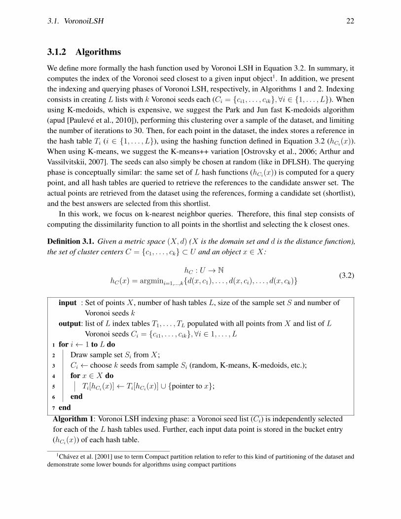
We define more formally the hash function used by Voronoi LSH in Equation 3.2. In summary, itcomputes the index of the Voronoi seed closest to a given input object1. In addition, we presentthe indexing and querying phases of Voronoi LSH, respectively, in Algorithms 1 and 2. Indexingconsists in creating L lists with k Voronoi seeds each (Ci = ci1, . . . , cik, ∀i ∈ 1, . . . , L). Whenusing K-medoids, which is expensive, we suggest the Park and Jun fast K-medoids algorithm(apud [Pauleve et al., 2010]), performing this clustering over a sample of the dataset, and limitingthe number of iterations to 30. Then, for each point in the dataset, the index stores a reference inthe hash table Ti (i ∈ 1, . . . , L), using the hashing function defined in Equation 3.2 (hCi
(x)).When using K-means, we suggest the K-means++ variation [Ostrovsky et al., 2006; Arthur andVassilvitskii, 2007]. The seeds can also simply be chosen at random (like in DFLSH). The queryingphase is conceptually similar: the same set of L hash functions (hCi
(x)) is computed for a querypoint, and all hash tables are queried to retrieve the references to the candidate answer set. Theactual points are retrieved from the dataset using the references, forming a candidate set (shortlist),and the best answers are selected from this shortlist.
In this work, we focus on k-nearest neighbor queries. Therefore, this final step consists ofcomputing the dissimilarity function to all points in the shortlist and selecting the k closest ones.
Definition 3.1. Given a metric space (X, d) (X is the domain set and d is the distance function),the set of cluster centers C = c1, . . . , ck ⊂ U and an object x ∈ X:
hC : U → NhC(x) = argmini=1,...,kd(x, c1), . . . , d(x, ci), . . . , d(x, ck)
(3.2)
input : Set of points X , number of hash tables L, size of the sample set S and number ofVoronoi seeds k
output: list of L index tables T1, . . . , TL populated with all points from X and list of LVoronoi seeds Ci = ci1, . . . , cik,∀i ∈ 1, . . . , L
for i← 1 to L do1
Draw sample set Si from X;2
Ci ← choose k seeds from sample Si (random, K-means, K-medoids, etc.);3
for x ∈ X do4
Ti[hCi(x)]← Ti[hCi
(x)] ∪ pointer to x;5
end6
end7
Algorithm 1: Voronoi LSH indexing phase: a Voronoi seed list (Ci) is independently selectedfor each of the L hash tables used. Further, each input data point is stored in the bucket entry(hCi
(x)) of each hash table.
1Chavez et al. [2001] use to term Compact partition relation to refer to this kind of partitioning of the dataset anddemonstrate some lower bounds for algorithms using compact partitions
3.1. VoronoiLSH 23
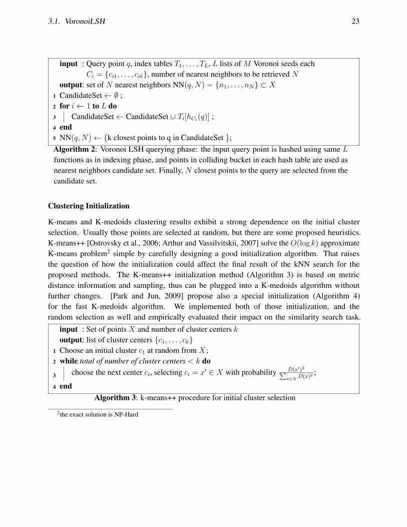
input : Query point q, index tables T1, . . . , TL, L lists of M Voronoi seeds eachCi = ci1, . . . , cik, number of nearest neighbors to be retrieved N
output: set of N nearest neighbors NN(q,N) = n1, . . . , nN ⊂ X
CandidateSet← ∅ ;1
for i← 1 to L do2
CandidateSet← CandidateSet ∪ Ti[hCi(q)] ;3
end4
NN(q,N)← k closest points to q in CandidateSet ;5
Algorithm 2: Voronoi LSH querying phase: the input query point is hashed using same Lfunctions as in indexing phase, and points in colliding bucket in each hash table are used asnearest neighbors candidate set. Finally, N closest points to the query are selected from thecandidate set.
Clustering Initialization
K-means and K-medoids clustering results exhibit a strong dependence on the initial clusterselection. Usually those points are selected at random, but there are some proposed heuristics.K-means++ [Ostrovsky et al., 2006; Arthur and Vassilvitskii, 2007] solve the O(log k) approximateK-means problem2 simple by carefully designing a good initialization algorithm. That raisesthe question of how the initialization could affect the final result of the kNN search for theproposed methods. The K-means++ initialization method (Algorithm 3) is based on metricdistance information and sampling, thus can be plugged into a K-medoids algorithm withoutfurther changes. [Park and Jun, 2009] propose also a special initialization (Algorithm 4)for the fast K-medoids algorithm. We implemented both of those initialization, and therandom selection as well and empirically evaluated their impact on the similarity search task.
input : Set of points X and number of cluster centers koutput: list of cluster centers c1, . . . , ckChoose an initial cluster c1 at random from X;1
while total of number of cluster centers < k do2
choose the next center ci, selecting ci = x′ ∈ X with probability D(x′)2∑x∈X
D(x)2 ;3
end4
Algorithm 3: k-means++ procedure for initial cluster selection
2the exact solution is NP-Hard

3.1. VoronoiLSH 24
input : Set of points X = x1, . . . , xn and expected number of cluster centers koutput: list of cluster centers c1, . . . , ckCalculate distance matrix with dij = d(xi, xj)n×n;1
for j ← 1 to n do2
vj ←∑ni=1 dij/
∑nl=1 dil ;3
end4
Sort v1, . . . , vn in ascending order;5
Select the k points with smallest vj value as initial cluster centers;6
Algorithm 4: Park and Jun procedure for initial cluster selection
3.1.3 Cost models and Complexity Aspects
We will consider two models for query cost, a more simplistic looking only to distance computationand another one taking into account other costs. We must remember that there is two basiccomponent of the query cost: the cost to find the appropriate bucket (called internal cost) and thecost to sequentially process and rank the points in the bucket (called external cost). The basicsupposition is that the number of points in a bucket can be approximated by its mean when weevaluate the average query cost.
Given a dataset X of n points and k centroids ci associated to a bucket Xi (which forms apartition of the dataset, implying that ∪Ki=1Xi = X and ∩Ki=1Xi = ∅), the average number of pointin a bucket (n) is given by:
n =∑Ki=1 |Xi|k
= n
k
For the fist model let us consider that the distance function evaluation is computationally muchmore expensive than any other computation in the algorithm, so the complexity is dominated bythe number of distance function evaluations. We denominate this cost model the Range SearchCost Model because it does not differentiate between range queries and k-nearest neighbor queriesin terms of cost. The internal cost is the number of distance computation in the linear scan forthe nearest centroid to the query and is fixed on k. The external cost is the number of distancecomputations for the final ranking. In the average case we will approximate this cost by the averagenumber of points n in each bucket. So the final cost is given by:
RC(n, k) = n
k+ k
Another possibility is to jointly analyze the final ranking cost, which does not depend solelyon the number of distance computations. For that matter, we assume that any basic operation(mathematical operators,numbers comparisons, memory transfer) has unit cost and that a givendistance has a constant cost of d > 1. We will denominate this model as Nearest-Neighbors CostModel. The final ranking operation has the complexity of a sorting algorithm, which is O(nlogn),

3.1. VoronoiLSH 25
over the average number of points in each bucket. Taking all into account the final cost is:
NNC(n, k, d) = n
klog(n
k) + d
n
k+ dk
Optimizing the parameters: VoronoiLSH has basically two parameters, the number of tablesL and number of centroids k. For the sake of simplicity we will look only for the parameter k(supposing a fixed L, and given that this parameter has a fixed multiplicative positive impact overthe query time complexity and a non-obvious multiplicative positive impact over the quality of thesearch).
Let us start with Range Search Model; Note that 1 ≤ k ≤ n and that in practical setups k n.
∂RC(n, k)∂k
= − n
k2 + 1 = 0
So the optimal number of centroids k is
⇒ k =√n
⇒ RC(n) = 2√n
For the Nearest-Neighbor Model we proceed in the same way, using the same assumptions:
∂NNC(n, k, d)∂k
= − n
k2 [log(nk
) + 1]− d nk2 + d = 0
⇒ n
k2 [log(nk
) + 1 + d] = d
So the optimal number of centroids k is implicit given by
k2 = n
d[log(n
k) + 1 + d]
Knowing that log(n/k) > 0 we conclude that
k2 >n
d(d+ 1)
⇒ n2
k2 <d
d+ 1n
⇒ log(nk
) < 12 log( d
d+ 1n)
⇒ n
d(d+ 1) < k2 = n
d[log(n
k) + 1 + d] < n
d[12 log( d
d+ 1n) + 1 + d]
⇒√n(1d
+ 1) < k <
√n[ 1
2d log( d
d+ 1n) + 1d
+ 1]

3.1. VoronoiLSH 26
⇒ d
√n(1d
+ 1) < dk < d
√n[ 1
2d log( d
d+ 1n) + 1d
+ 1]
⇒√n(d+ 1) < dk <
√n[12 log( d
d+ 1n) + d+ 1]
⇒ 1/√n[ 1
2d log( d
d+ 1n) + 1d
+ 1] < 1/k < 1/√n(1d
+ 1)
⇒ n√n[ 1
2d log( dd+1n) + 1
d+ 1]
< n/k <n√
n(1d
+ 1)
⇒√√√√ dn
12 log( d
d+1n) + d+ 1< n/k <
√dn
d+ 1
Knowing that the optimal k must satisfy
kd = n
klog n
k+ d
n
k+ n
k
⇒ kd− n
k= n
klog n
k+ d
n
k
We conclude that the optimal cost NNCopt(n, d) = NNC(n, k, d) may be simplified to
NNCopt(n, d) = 2dk + (d− 1)nk
Implying that
√nd[2√d+ 1+
√√√√√ (d− 1)2
log(√
dnd+1) + d+ 1
] < NNCopt(n, d) <√nd[2
√√√√log(√
dn
d+ 1) + d+ 1+√
(d− 1)2
d+ 1 ]
⇒ NNCopt(n, d) = O(√nd(log(
√n) + d+ 1) = O(d
√n(log(
√n) + 1
d+ 1)
In the Nearest-Neighbor cost model the dimensionality information is built-in the distance costd, for instance, if we consider Lp distance in a D dimensional Euclidean space, the distance costd may be approximated by dimensionality D. It is interesting to note that, although we did notachieve a logarithm query cost, we obtained a sub-linear cost on the number of points (and linearon the distance cost) which does not hide exponential costs on the dimensionality. Comparingto standard LSH in Euclidean space which solves the (c, r)-approximate nearest-neighbors withO(dnρ) query complexity, where d is the dimensionality (and the approximate cost of evaluating thedistance function) and ρ is a fractional power (depending on the approximation factor c) [Indyk andMotwani, 1998; Andoni and Indyk, 2006; Datar et al., 2004], we may conclude that the expectedquery complexity (under reasonable assumptions) are very close to the Euclidean LSH. However
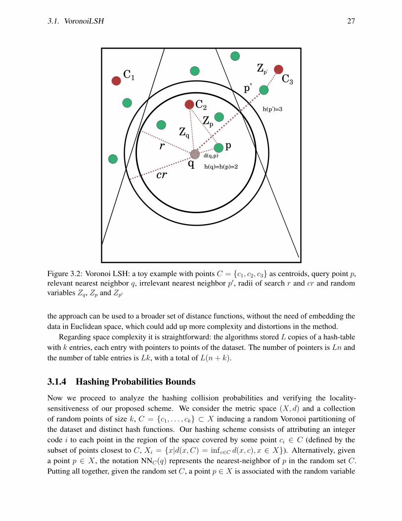
3.1. VoronoiLSH 27
C1
C2
C3
qr
cr
Zqp
Zp
d(q,p)
h(q)=h(p)=2
p'
h(p')=3
Zp'
Figure 3.2: Voronoi LSH: a toy example with points C = c1, c2, c3 as centroids, query point p,relevant nearest neighbor q, irrelevant nearest neighbor p′, radii of search r and cr and randomvariables Zq, Zp and Zp′
the approach can be used to a broader set of distance functions, without the need of embedding thedata in Euclidean space, which could add up more complexity and distortions in the method.
Regarding space complexity it is straightforward: the algorithms stored L copies of a hash-tablewith k entries, each entry with pointers to points of the dataset. The number of pointers is Ln andthe number of table entries is Lk, with a total of L(n+ k).
3.1.4 Hashing Probabilities Bounds
Now we proceed to analyze the hashing collision probabilities and verifying the locality-sensitiveness of our proposed scheme. We consider the metric space (X, d) and a collectionof random points of size k, C = c1, . . . , ck ⊂ X inducing a random Voronoi partitioning ofthe dataset and distinct hash functions. Our hashing scheme consists of attributing an integercode i to each point in the region of the space covered by some point ci ∈ C (defined by thesubset of points closest to C, Xi = x|d(x,C) = infc∈C d(x, c), x ∈ X). Alternatively, givena point p ∈ X , the notation NNC(q) represents the nearest-neighbor of p in the random set C.Putting all together, given the random set C, a point p ∈ X is associated with the random variable
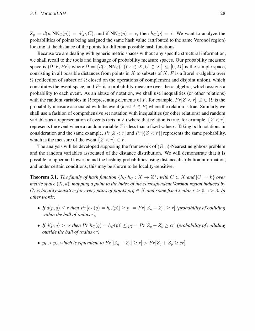
3.1. VoronoiLSH 28
Zp = d(p,NNC(p)) = d(p, C), and if NNC(p) = ci then hC(p) = i. We want to analyze theprobabilities of points being assigned the same hash value (attributed to the same Voronoi region)looking at the distance of the points for different possible hash functions.
Because we are dealing with generic metric spaces without any specific structural information,we shall recall to the tools and language of probability measure spaces. Our probability measurespace is (Ω, F, Pr), where Ω = d(x,NNC(x))|x ∈ X,C ⊂ X ⊆ [0,M ] is the sample space,consisting in all possible distances from points in X to subsets of X , F is a Borel σ-algebra overΩ (collection of subset of Ω closed on the operations of complement and disjoint union), whichconstitutes the event space, and Pr is a probability measure over the σ-algebra, which assigns aprobability to each event. As an abuse of notation, we shall use inequalities (or other relations)with the random variables in Ω representing elements of F , for example, Pr[Z < r], Z ∈ Ω, is theprobability measure associated with the event (a set A ∈ F ) where the relation is true. Similarly weshall use a fashion of comprehensive set notation with inequalities (or other relations) and randomvariables as a representation of events (sets in F ) where that relation is true, for example, Z < rrepresents the event where a random variable Z is less than a fixed value r. Taking both notations inconsideration and the same example, Pr[Z < r] and Pr[Z < r] represents the same probability,which is the measure of the event Z < r ∈ F .
The analysis will be developed supposing the framework of (R, c)-Nearest neighbors problemand the random variables associated of the distance distribution. We will demonstrate that it ispossible to upper and lower bound the hashing probabilities using distance distribution information,and under certain conditions, this may be shown to be locality-sensitive.
Theorem 3.1. The family of hash function hC |hC : X → Z+, with C ⊂ X and |C| = k overmetric space (X, d), mapping a point to the index of the correspondent Voronoi region induced byC, is locality-sensitive for every pairs of points p, q ∈ X and some fixed scalar r > 0, c > 3. Inother words:
• If d(p, q) ≤ r then Pr[hC(q) = hC(p)] ≥ p1 = Pr[|Zq − Zp| ≥ r] (probability of collidingwithin the ball of radius r),
• If d(p, q) > cr then Pr[hC(q) = hC(p)] ≤ p2 = Pr[Zq + Zp ≥ cr] (probability of collidingoutside the ball of radius cr)
• p1 > p2, which is equivalent to Pr[|Zq − Zp| ≥ r] > Pr[Zq + Zp ≥ cr]
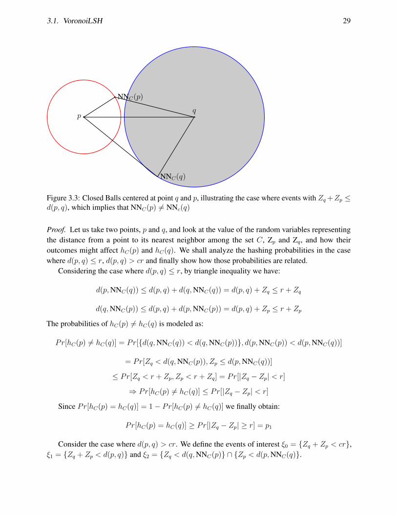
3.1. VoronoiLSH 29
pq
NNC(p)
NNC(q)
Figure 3.3: Closed Balls centered at point q and p, illustrating the case where events with Zq +Zp ≤d(p, q), which implies that NNC(p) 6= NNc(q)
Proof. Let us take two points, p and q, and look at the value of the random variables representingthe distance from a point to its nearest neighbor among the set C, Zp and Zq, and how theiroutcomes might affect hC(p) and hC(q). We shall analyze the hashing probabilities in the casewhere d(p, q) ≤ r, d(p, q) > cr and finally show how those probabilities are related.
Considering the case where d(p, q) ≤ r, by triangle inequality we have:
d(p,NNC(q)) ≤ d(p, q) + d(q,NNC(q)) = d(p, q) + Zq ≤ r + Zq
d(q,NNC(p)) ≤ d(p, q) + d(p,NNC(p)) = d(p, q) + Zp ≤ r + Zp
The probabilities of hC(p) 6= hC(q) is modeled as:
Pr[hC(p) 6= hC(q)] = Pr[d(q,NNC(q)) < d(q,NNC(p)), d(p,NNC(p)) < d(p,NNC(q))]
= Pr[Zq < d(q,NNC(p)), Zp ≤ d(p,NNC(q))]
≤ Pr[Zq < r + Zp, Zp < r + Zq] = Pr[|Zq − Zp| < r]
⇒ Pr[hC(p) 6= hC(q)] ≤ Pr[|Zq − Zp| < r]
Since Pr[hC(p) = hC(q)] = 1− Pr[hC(p) 6= hC(q)] we finally obtain:
Pr[hC(p) = hC(q)] ≥ Pr[|Zq − Zp| ≥ r] = p1
Consider the case where d(p, q) > cr. We define the events of interest ξ0 = Zq + Zp < cr,ξ1 = Zq + Zp < d(p, q) and ξ2 = Zq < d(q,NNC(p) ∩ Zp < d(p,NNC(q).
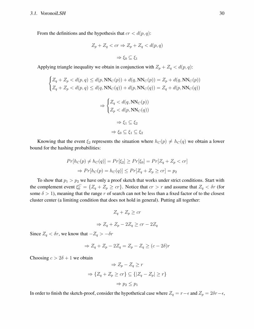
3.1. VoronoiLSH 30
From the definitions and the hypothesis that cr < d(p, q):
Zp + Zq < cr ⇒ Zp + Zq < d(p, q)
⇒ ξ0 ⊆ ξ1
Applying triangle inequality we obtain in conjunction with Zp + Zq < d(p, q):
Zq + Zp < d(p, q) ≤ d(p,NNC(p)) + d(q,NNC(p)) = Zp + d(q,NNC(p))Zq + Zp < d(p, q) ≤ d(q,NNC(q)) + d(p,NNC(q)) = Zq + d(p,NNC(q))
⇒
Zq < d(q,NNC(p))Zp < d(p,NNC(q))
⇒ ξ1 ⊆ ξ2
⇒ ξ0 ⊆ ξ1 ⊆ ξ2
Knowing that the event ξ2 represents the situation where hC(p) 6= hC(q) we obtain a lowerbound for the hashing probabilities:
Pr[hC(p) 6= hC(q)] = Pr[ξ2] ≥ Pr[ξ0] = Pr[Zq + Zp < cr]
⇒ Pr[hC(p) = hC(q)] ≤ Pr[Zq + Zp ≥ cr] = p2
To show that p1 > p2 we have only a proof sketch that works under strict conditions. Start withthe complement event ξC0 = Zq + Zp ≥ cr. Notice that cr > r and assume that Zq < δr (forsome δ > 1), meaning that the range r of search can not be less than a fixed factor of to the closestcluster center (a limiting condition that does not hold in general). Putting all together:
Zq + Zp ≥ cr
⇒ Zq + Zp − 2Zq ≥ cr − 2Zq
Since Zq < δr, we know that −Zq > −δr
⇒ Zq + Zp − 2Zq = Zp − Zq ≥ (c− 2δ)r
Choosing c > 2δ + 1 we obtain⇒ Zp − Zq ≥ r
⇒ Zq + Zp ≥ cr ⊆ |Zq − Zp| ≥ r
⇒ p2 ≤ p1
In order to finish the sketch-proof, consider the hypothetical case where Zq = r−ε and Zp = 2δr−ε,

3.2. VoronoiPlex LSH 31
for an arbitrary ε > 0 (and maintaining the previous assumptions on δ and c). Taking Zp − Zq, weobtain 2δr − ε − r + ε = (2δ − 1)r, meaning that |Zq − Zp| > r (Zp and Zq are elements of theevent |Zq−Zp| ≥ r). Computing Zp +Zq = 2δr− ε+ r− ε, we obtain (2δ+ 1)r− 2ε, implyingthat Zq + Zp < (2δ + 1)r; Since (2δ + 1) < c (an assumption from the previous step of the proof),we obtain Zq + Zp < cr , and conclude that Zq + Zp ≥ cr is a proper subset of |Zq − Zp| ≥ runder the conditions we are analyzing.
⇒ p2 < p1
This is a generic result depending on some assumptions of the metric structure of the space anda somehow reasonable workload of the (r, c)-ANN, but does not elucidate relationships betweenthe choice of variable (namely k and L) and the probabilistic guarantees of the method. Furtherdevelopment in this line of argument is possible by observing that the distribution of the randomvariables Zq and Zp may be understood as an order statistics over the distribution of distances inthe dataset. Indeed if we define the (unordered) sequence of random variable Zq(1), · · · , Zq(k) asdistances from q ∈ X to a each point c1, · · · , ck from a random sample C ⊆ X (|C| = k), therandom variable Zq correspond to the order statistics min(Zq(1), · · · , Zq(k)). We may compute thecumulative distribution function (cdf) Fmin of the minimum order statistics using the hypothesisthat the random variables Zq(1), · · · , Zq(k) are i.i.d. (a not unrealistic one, given that the sample C israndomly chosen from the original dataset) and are distributed according to a cdf F :
Fmin(x) = P (Zq ≤ x) = P (min(Zq(1), · · · , Zq(k)) ≤ x) = 1− P (min(Zq(1), · · · , Zq(k)) > x)
= 1− P (Zq(1) > x, · · · , Zq(k) > x) = 1−i=k∏i=1
P (Zq(i) > x) = 1−i=k∏i=1
(1− F (x))
⇒ Fmin(x) = 1− (1− F (x))k
The interesting fact about this relation is that somehow, without using the “concatenation”trick (building a composite LSH hash using the concatenation of multiple LSH, implying in themultiplication of the hashing probabilities), we achieved a similar exponential probability for thenearest-neighbor distance probability from the distance distribution.
3.2 VoronoiPlex LSH
VoronoiLSH was our first attempt to develop a LSH family for general metric space, seeking goodtrade-off between effectiveness, efficiency and generalization. We took a very simplistic design,and as we have presented in the theoretical characterization of the method, despite the minimalisticapproach (in relation the other methods that directly apply various metric space properties forfiltering and pruning) the method achieves competitive average query time performance and can be
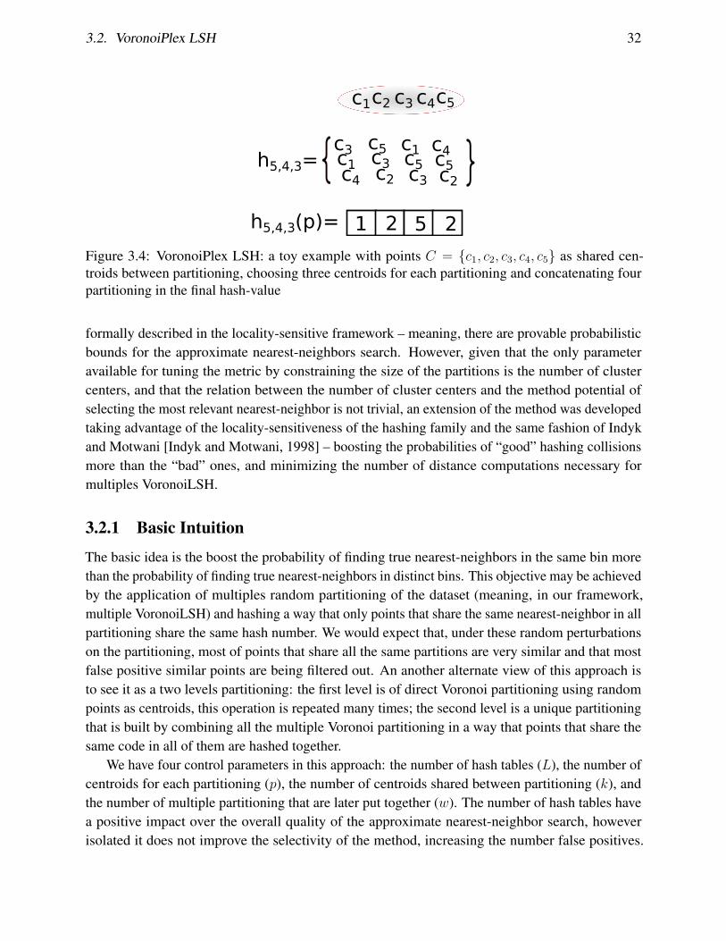
3.2. VoronoiPlex LSH 32
1 2 5 2
c1c2 c3 c4c5
c1c3c4
c3c5c2
c5c1c3
c5c4c2
h5,4,3=
h5,4,3(p)=
Figure 3.4: VoronoiPlex LSH: a toy example with points C = c1, c2, c3, c4, c5 as shared cen-troids between partitioning, choosing three centroids for each partitioning and concatenating fourpartitioning in the final hash-value
formally described in the locality-sensitive framework – meaning, there are provable probabilisticbounds for the approximate nearest-neighbors search. However, given that the only parameteravailable for tuning the metric by constraining the size of the partitions is the number of clustercenters, and that the relation between the number of cluster centers and the method potential ofselecting the most relevant nearest-neighbor is not trivial, an extension of the method was developedtaking advantage of the locality-sensitiveness of the hashing family and the same fashion of Indykand Motwani [Indyk and Motwani, 1998] – boosting the probabilities of “good” hashing collisionsmore than the “bad” ones, and minimizing the number of distance computations necessary formultiples VoronoiLSH.
3.2.1 Basic Intuition
The basic idea is the boost the probability of finding true nearest-neighbors in the same bin morethan the probability of finding true nearest-neighbors in distinct bins. This objective may be achievedby the application of multiples random partitioning of the dataset (meaning, in our framework,multiple VoronoiLSH) and hashing a way that only points that share the same nearest-neighbor in allpartitioning share the same hash number. We would expect that, under these random perturbationson the partitioning, most of points that share all the same partitions are very similar and that mostfalse positive similar points are being filtered out. An another alternate view of this approach isto see it as a two levels partitioning: the first level is of direct Voronoi partitioning using randompoints as centroids, this operation is repeated many times; the second level is a unique partitioningthat is built by combining all the multiple Voronoi partitioning in a way that points that share thesame code in all of them are hashed together.
We have four control parameters in this approach: the number of hash tables (L), the number ofcentroids for each partitioning (p), the number of centroids shared between partitioning (k), andthe number of multiple partitioning that are later put together (w). The number of hash tables havea positive impact over the overall quality of the approximate nearest-neighbor search, howeverisolated it does not improve the selectivity of the method, increasing the number false positives.

3.2. VoronoiPlex LSH 33
The other three parameters have a non-trivial impact in selectivity and quality of the search thatwe still need to further investigate. In the following sections, we will present a brief theoreticalcharacterization of this impact. Figure 3.4 presents an example with five shared centroids (k = 5),four partitioning concatenated (w = 4) and three centroids in each partitioning (p = 3).
3.2.2 Algorithms
The algorithms for indexing and kNN searching are essentially the same described in Algorithm 1and Algorithm 2, with the exception of the hash function. Hence, we will present the algorithm forthe construction of the hash function and for the application of the hashing to a point in the metricspace. We will assume that functions/methods are first class objects with the possibility of beingreturned from a method, encapsulating data and computation.
Algorithm 5 performs a multiple selection of index and stores the selected indexes in a datastructure that represents the hashing function. The indexes selected are used as sub-samples of agiven sample of the dataset, and each group of selected indexes forms a set of centroid points thatspans a Voronoi partitioning of the space. Those k partitioning forms a product space of hash-vectorsof size k. The intuitive idea is to build up on the VoronoiLSH intuition, using the compact closestcenter relation as a hashing function, and with a bounded number of distance computation, constructa product space of hash function. The idea is to boost the single hash probabilities with a controllednumber of distance of computation.
input : Integer size k of the sample C = c1, . . . , ck ⊂ X , integer number of distinctpartitioning w, and integer number of centroids for each partitioning p < k
output: A hash function hk,w,p object with two arrays indicating the random choice ofcentroids made by the method
selected← new binary array of size k;1
subsample← new integer multi-array of size w × p;2
for j ← 1 to w do3
Random sample S = s1, · · · , sp from 1, · · · , k;4
for i← 1 to p do5
subsample[j, i]← si;6
selected[si]← 1;7
end8
end9
hk,w,p ← (selected,subsample) ;10
Algorithm 5: Hash function building

3.2. VoronoiPlex LSH 34
input : Hash function object hk,w,p,Sample C = c1, . . . , ck ⊂ X (|C| = k) and a pointq ∈ X
output: Integer value hk,w,p(q)(selected,subsample)← retrieved from hk,w,p distances← new floating-point array of size k;1
for j ← 1 to k do2
if selected[j] == 1 then3
distances[j]← d(q, cj) ;4
end5
end6
hasharray← new integer array of size w;7
for i← 1 to w do8
hasharray[i]← element in subsample[i] that minimize distances[j] (varying j) ;9
end10
hk,w,p(q)← hash(hasharray) ;11
Algorithm 6: Hash function Application
3.2.3 Theoretical characterization
First, we must note that the hash function build procedure (Algorithm 5) is blind to the actualdata. It is a random selection of indexes of the arrays that store the sampled points. So in firstsight we can see that it could be precomputed, or at least re-used in various distinct settings of thealgorithm (for example, in a distributed memory system, there could be strong re-utilization of thehash functions). The algorithm consist of two “for” loops and a simple random sample in a set ofk elements, resulting in a time complexity of O(w(p+ k)) and a space complexity of O(k + wp)(with size k of the sample C = c1, . . . , ck ⊂ X , integer number of distinct partitioning w, andinteger number of centroids for each partitioning p < k).
For the time complexity we will continue with the focus on expensive computation bottlenecks –distance computation. The discussion will be focused on the expected number of positions in theselected array that are set to one – IEi=1,··· ,k[selected[i] = 1].
Proposition 3.1. After w rounds of the outer “for” loop in Algorithm 5, the expected number ofposition of the array selected set to one is IEi=1,··· ,k[selected[i] = 1] = k − k(1− p
k)w.
Proof. Start with the probability of a specific position being assigned 1 in a single iteration of the
for loop. There are(k
p
)possible ways of sampling p values from k. There are
(k − 1p
)ways of
sampling p values of k excluding some value of the set with size k. So, the number of ways of

3.3. Parallel VoronoiLSH 35
sampling p and not assigning selected[i] one of them is(k − 1p
). Putting all together:
Prsingle iteration[selected[i] = 1] = 1−
(k − 1p
)(k
p
) = p
k
After w iteration, the probability of the position i not being assigned to 1 is multiplication of theprobabilities of not being assigned at each iteration.
Prafter w iteration[selected[i] 6= 1] =w∏n=1
Prsingle iteration[selected[i] 6= 1]
Prafter w iteration[selected[i] 6= 1] = (1− p
k)w
⇒ Prafter w iteration[selected[i] = 1] = 1− (1− p
k)w
Using the probability of being assigned after w iterations of the for loop, we calculate the finalexpectation of the number of elements in the array selected that are assigned to 1.
IEi=1,··· ,k[selected[i] = 1] = kPrafter w iteration[selected[i] = 1]
IEi=1,··· ,k[selected[i] = 1] = k − k(1− p
k)w
This result is important because it helps us understand how the number of distance computation(and the internal cost) of the hashing algorithm is bounded using the parameters that the hashfunction is build and taking into account the randomness of the building algorithm. So in generalthe internal cost, looking only for the number of distance computation is O(k − kε) where this εfactor is well related with the effectiveness of the search.
3.3 Parallel VoronoiLSH
The design and adaptation of the original sequential algorithm for a distributed and parallel frame-work was developed through a collaborative work of the author, Prof. Eduardo Valle, Prof. GeorgeTeodoro and Thiago Teixeira. George Teodoro and Thiago Teixeira work is specialized in distributedsystems and they developed substantial part of the parallelization, specially the implementation us-ing dataflow programming paradigm and performance test in a distributed cluster. This collaborationresulted in an conference paper accepted at SISAP2014.
The parallelization strategy we employ is based on the dataflow programming paradigm [Arpaci-Dusseau et al., 1999; Beynon et al., 2001; Teodoro et al., 2008]. Dataflow applications are typically
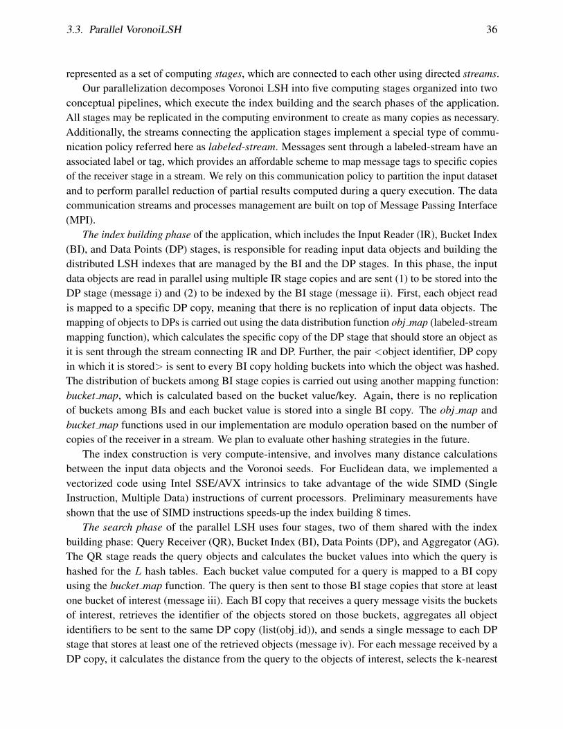
3.3. Parallel VoronoiLSH 36
represented as a set of computing stages, which are connected to each other using directed streams.Our parallelization decomposes Voronoi LSH into five computing stages organized into two
conceptual pipelines, which execute the index building and the search phases of the application.All stages may be replicated in the computing environment to create as many copies as necessary.Additionally, the streams connecting the application stages implement a special type of commu-nication policy referred here as labeled-stream. Messages sent through a labeled-stream have anassociated label or tag, which provides an affordable scheme to map message tags to specific copiesof the receiver stage in a stream. We rely on this communication policy to partition the input datasetand to perform parallel reduction of partial results computed during a query execution. The datacommunication streams and processes management are built on top of Message Passing Interface(MPI).
The index building phase of the application, which includes the Input Reader (IR), Bucket Index(BI), and Data Points (DP) stages, is responsible for reading input data objects and building thedistributed LSH indexes that are managed by the BI and the DP stages. In this phase, the inputdata objects are read in parallel using multiple IR stage copies and are sent (1) to be stored into theDP stage (message i) and (2) to be indexed by the BI stage (message ii). First, each object readis mapped to a specific DP copy, meaning that there is no replication of input data objects. Themapping of objects to DPs is carried out using the data distribution function obj map (labeled-streammapping function), which calculates the specific copy of the DP stage that should store an object asit is sent through the stream connecting IR and DP. Further, the pair <object identifier, DP copyin which it is stored> is sent to every BI copy holding buckets into which the object was hashed.The distribution of buckets among BI stage copies is carried out using another mapping function:bucket map, which is calculated based on the bucket value/key. Again, there is no replicationof buckets among BIs and each bucket value is stored into a single BI copy. The obj map andbucket map functions used in our implementation are modulo operation based on the number ofcopies of the receiver in a stream. We plan to evaluate other hashing strategies in the future.
The index construction is very compute-intensive, and involves many distance calculationsbetween the input data objects and the Voronoi seeds. For Euclidean data, we implemented avectorized code using Intel SSE/AVX intrinsics to take advantage of the wide SIMD (SingleInstruction, Multiple Data) instructions of current processors. Preliminary measurements haveshown that the use of SIMD instructions speeds-up the index building 8 times.
The search phase of the parallel LSH uses four stages, two of them shared with the indexbuilding phase: Query Receiver (QR), Bucket Index (BI), Data Points (DP), and Aggregator (AG).The QR stage reads the query objects and calculates the bucket values into which the query ishashed for the L hash tables. Each bucket value computed for a query is mapped to a BI copyusing the bucket map function. The query is then sent to those BI stage copies that store at leastone bucket of interest (message iii). Each BI copy that receives a query message visits the bucketsof interest, retrieves the identifier of the objects stored on those buckets, aggregates all objectidentifiers to be sent to the same DP copy (list(obj id)), and sends a single message to each DPstage that stores at least one of the retrieved objects (message iv). For each message received by aDP copy, it calculates the distance from the query to the objects of interest, selects the k-nearest

3.4. Final remarks 37
neighbor objects to the query, and sends those local NN objects to the AG stage. Finally, the AGstage receives the message containing the DPs local NN objects from all DPs involved in that querycomputation and performs a reduction operation to compute the global NN objects. The DP copies(message v) use the query id as a label to the message, guaranteeing that the same AG copy willprocess all messages related to a specific query. As a consequence, multiple AG copies may becreated to execute different queries in parallel. Although we have presented the index building andthe search as sequential phases for sake of simplicity, their executions may overlap.
The parallelization approach we have proposed exploits task, pipeline, replicated and intra-stageparallelism. Task parallelism results from concurrent execution that allows indexing and searchingphases to overlap, e.g. during an update of the index. Pipeline parallelism occurs as the searchstages, for instance, execute different queries in parallel in a pipeline fashion. Replicated parallelismis available in all stages of the application, which may have an arbitrary number of copies. Finally,intra-stage parallelism results of the application’s ability to use multiple cores within a stage copy.This parallelism has the advantages of sharing the same memory space among computing cores in astage copy, and a reduced number of messages exchanged, since a smaller number of state partitionsmay be used.
3.4 Final remarks
We have demonstrated that using only metric space properties it is possible to design a LSH familyof function over general metric space, using a form of compact partition relation (inducing apartitioning of the space in Dirichlet domains). Our mathematical proof is an original contributionand one of the main contribution of this dissertation. However we should see experimentally howthis approach is comparable to other similar methods in the literature. We will accomplish thiscomparison in the next chapter.

Chapter 4
Experiments
In this chapter the experimental data generated during this research is reported and discussed. Thisis a recollection of at least four distinct groups of experiments performed in two years of research.Since the development of the algorithms, and specially the parameters of the algorithms was donein a cycle of theories, hypothesis and tests, the experimental data reported here is not homogeneousnor along the datasets, neither along the methods. So for the case of Euclidean data, we compare theperformance of our proposed methods with the performance of K-Means LSH. When we are dealingwith metric data, K-Means LSH can not be directly applied (only with an additional embedding,which is not the intent of this work), so we compare with another version of LSH for metric space(BPI). In the large scale experiment our intent was not to compare with other methods, but evaluateif the effectiveness and efficiency reported in the sequential small scale setup would scale-up in adistributed framework.
4.1 Datasets
For the experiments regarding Euclidean Spaces and Image Retrieval we resorted to the APMdataset (Arquivo Publico Mineiro – The Public Archives in Minas Gerais) which was created fromthe application of various transformation (15 transformation of scale, rotation, etc) to 100 antiquephotographs of the Public Archives of Minas Gerais. The SIFT descriptors of each transformedimage were calculated, resulting in a dataset of 2.871.300 feature vectors (SIFT descriptor is a 128dimensional vector). The queries dataset is build from the SIFT descriptors of the original images (atotal of 263.968 feature vectors). Each query point is equipped with its set of true nearest neighbors– the ground-truth. For these experiments we used 5000 points uniformly sampled from the querydataset and performed a 10-NN search.
In order to evaluate the case of general metric space we resorted to English dictionary of stringsand Listeria Genes string datasets with Levenshtein distance from SISAP Metric Library [Figueroaet al., 2007]. The English dataset has 69,069 strings, 500 strings are randomly removed from theset to serve as query dataset. In Figure 4.1 there are summarized information and graph regardingstring length distribution in those metric datasets. String length distribution affects directly for the
38

4.2. Techniques Evaluated 39
Levenshtein distance calculation (quadratic on the string length).We used BigAnn [Jegou et al., 2011] dataset for the large scale experiment. The BigAnn contains
a thousand million (109) 128-dimensional SIFT local feature vectors extracted from images, and10,000 query feature vectors. Euclidean distance is used for SIFT. We perform kNN searches, withk=5, 10, and 30 for the Dictionary and Listeria dataset, and k=10 for the BigAnn dataset.
0 1000 2000 3000 4000 5000 6000 7000
string length
0.00
0.02
0.04
0.06
0.08
0.10
0.12
norm
alize
d f
req
uen
cy
Listeria genesMean word len = 902.220958374Var word len = 402821.134285
(a)
0 5 10 15 20 25
string length
0.0
0.1
0.2
0.3
0.4
0.5
norm
alize
d f
req
uen
cy
English dictionaryMean word len = 8.40022296544
Var word len = 6.4408292659
(b)
Figure 4.1: (a) Listeria Gene Dataset string length distribution (b) English Dataset string lengthdistribution
4.2 Techniques Evaluated
K-means LSH, Voronoi LSH and DFLSH: In order to evaluate the feasibility of Voronoi LSH(using K-Medoids) we compared it with the K-means LSH et al. [Pauleve et al., 2010] and theDFLSH [Kang and Jung, 2012]. Although all three methods may be described as Voronoi LSH, butwith distinct centroid selection heuristics, the distinction we are making here (between Voronoi,K-Means and DFLSH) serve the purpose of investigating the trade-offs present in the choice ofclustering k
We implemented all the methods in the same framework, namely Java and The ApacheCommonsTM Mathematics Library1. K-means LSH is used as a baseline method, since its per-formance and behavior are well studied and presented in the literature and DFLSH is an alternativemethod for the same problem.
VoronoiLSH and Brief-Permutation Index LSH : In order to allow the comparison with BPILSH, we followed an experiment protocol as close as possible to the one described in their paper,and used the recall and query runtime reported there. In order to remove the effects of differencesin implementation details and execution environment, we normalize both methods runtime by the
1 Commons Math: The Apache Commons Mathematics Library, accessed in 22/09/2013. http://commons.apache.org/proper/commons-math/

4.3. Evaluation Metrics 40
respective brute-force linear scan runtime. Because the authors report their numbers graphically, weadded error bars to indicate the imprecision of our reading of their results.
Large-scale experiment : in this case the most important aspect to evaluate is the algorithmspeed up in the distributed configuration scaling-up the number of nodes and processors.
4.3 Evaluation Metrics
Given a query point q, we denote N(q, k) the set of true relevant k-nearest neighbors, A(q) the setof candidate nearest neighbors (shortlist) and R(q, k) the set of k-nearest neighbors returned by thealgorithm. We are concerned especially with the relations between the recall and extensivenessmetric given the variation in the parametric space of the methods. The recall metric is the fractionof total correct answers over the number of true relevant answers (Equation 4.1). The extensivenessmetric is the fraction of the dataset selected for the shortlist processing (Equation 4.2). The relatedselectivity metric (Equation 4.3) has distinct (and sometimes conflicting) use in the database andimage communities.
We employ the recall as a metric of quality, and the extensiveness as metric of cost for thetechniques. The recall is defined as usual for information retrieval, as the fraction of relevant answersthat was effectively retrieved. The extensiveness metric is the fraction of the dataset selected into theshortlist for linear scan. As the indexes work by selecting a (hopefully small) fraction of the datasetas candidates, and then computing the actual distance to the query for those candidates, the size ofthe shortlist corresponds to the number of distances computed for that query. The related selectivitymetric (selectivity = 1− extensivity) has distinct (and sometimes conflicting) use in the databaseand image retrieval research communities: some authors used it as a synonymous for extensiveness,while others and we use it as a complementary notion (as selectivity grows, extensivity drops).We also employ the query runtime as metric of cost. Runtime metrics are difficult to compareacross the literature, due to differences in code optimization, programming language, and executionenvironment, but in controlled experiments like ours they can offer a perspective on the cost ofdifferent techniques.
Given a query point q, we denote N(q, k) the set of true relevant k-nearest neighbors, A(q) theset of candidate nearest neighbors (shortlist) and R(q, k) the set of k-nearest neighbors returned bythe algorithm we define the recall, extensivity and selectivity metrics in Equation 4.1, Equation 4.2and Equation 4.3.
recall(q) = |R(q, k)||N(q, k)| (4.1)
extensiveness(q) = |A(q)|n
(4.2)
selectivity(q) = 1− |A(q)|n
(4.3)

4.4. Results 41
4.4 Results
In the next section we will present our experimental results separated by datasets and methods. Inthe Section 4.4.1 we will present the results using the APM dataset (Euclidean) which permits us acomparison with K-Means LSH, since K-Means algorithm depends and uses specific coordinateinformation that are not always available in generic metric spaces. In Section 4.4.2 the metricdataset of words in English is used. Since the same dataset is used for reporting the results ofBrief-Permutation Index LSH, we use it for comparison of this alternative formulation of LSHin metric spaces. It was shown in Figure 4.1 that the English dictionary is more easily processedbecause of the limited and low length of the words, in the Listeria dataset the situation is muchmore complicated because of the large variability and average lengths of words. We report resultsof DFLSH and VoronoiPlex-LSH in this settings in Section 4.4.3. Finally in Section 4.4.4 theresults of the distributed large scale experiment using BigANN dataset (One billion of points of124-dimensional euclidean points) are reported.

4.4. Results 42
4.4.1 APM Dataset: comparison with K-Means LSH
0.62
0.64
0.66
0.68
0.7
0.72
0.74
0.76
0.78
0.8
0.82
0.001 0.01 0.1 1
recall
extensiveness
DFLSHK-MedoidsLSHK-MeansLSH
(a) Recall x Extensiveness (log scale)
0.6
0.65
0.7
0.75
0.8
0.85
0.9
0.95
1
0 0.005 0.01 0.015 0.02 0.025 0.03
recall
extensiveness
DFLSHK-MedoidsLSHK-MeansLSH
L=1
L=5
L=8
(b) Recall x Number of hash functions L, Extensiveness (for 5000 cluster centers)
Figure 4.2: APM Dataset: Comparison of VoronoiLSH with three centroids selections strategyK-means, K-medoids and Random for 10-NN

4.4. Results 43
0
0.02
0.04
0.06
0.08
0.1
0.12
0.14
0.16
0.18
0 1000 2000 3000 4000 5000 6000 7000 8000 9000 10000
extensive
nes
s
#of cluster centers
DFLSHK-MedoidsLSHK-MeansLSH
(a) Extensiveness x Number of cluster centers
-0.01
0
0.01
0.02
0.03
0.04
0.05
0.06
0 0.02 0.04 0.06 0.08 0.1 0.12 0.14 0.16
differenceofrecall
extensiveness
K-means LSH-DFLSHK-medoids LSH-DFLSH
(b) Difference of Recall (Using DFLSH as a baseline) x Extensiveness
Figure 4.3: APM Dataset: Comparison of the impact of the number of cluster center in theextensivity metric and the correlation between extensivity and the recall for K-means LSH, VoronoiLSH and DFLSH (10-NN)
Figure 4.2a presents results relating recall with extensiveness. Notice that high extensivenessmeans that a large part of the dataset is being processed in the final sequential ranking – that isnot a desirable point of operation, since the main performance bottleneck on the query processingtime is located at that stage. For an extensiveness as low as 0.3%, both methods’ recall metric isapproximately 65% and with 1% extensiveness the recall grows up to a 80%. These results could be

4.4. Results 44
improved by using more than one hash function (Figure 4.2b) . Clearly K-means LSH presents thebest result on the recall metric, however it is important to notice that both DFLSH and Voronoi LSHare not exploiting any vector coordinate properties, relying solely on distance information, and aretherefore more general.
There seems to be a trade-off between number of cluster centers, number of hash functions andselectivity. In Figure 4.2b we see a comparison of recall and extensiveness for a varying number ofhash functions. We observe results indicating that in some setups Voronoi LSH and DFLSH mayoffer a better trade-off between quality of the response and selectivity than K-means LSH. It is notclear what specific feature of those methods may trigger this improvement, but nonetheless it isa very interesting result and may offer some precious intuition on the design of metric indexingmethods and choice of parameters.
Although K-means LSH attained the best results with a single hash table, the performance ofVoronoi LSH and DFLSH is comparatively better as the number of hash tables used increase (SeeFigure 4.2b). As shown, in some setups Voronoi LSH and DFLSH may offer a better trade-offbetween recall and selectivity than K-means LSH. For instance, for a recall of about 95% (L=5)Voronoi LSH and K-means have extensiveness of nearly 0.013 and 0.018, respectively. In otherwords, our method has to evaluate about 28% less elements in the final ranking phase. A similarlevel of comparative performance is attained when with a recall of about 97% (L=8). In comparisonto DFLSH, our method attained better performance in all setups. The extensiveness results are veryimportant because the final ranking phase represents one of the bottlenecks of searching algorithms.
There is a strong linear correlation between query time and selectivity. Fitting this to a linearmodel we obtain a very significant and well-adjusted linear model (R2 = 0.9985, p-value <2.2×10⁻¹⁵), with a linear coefficient of 17756.205 for the extensiveness and an intercept coefficientof −2.274. Other noticeable strong correlation appears between selectivity and number of clustercenters (Figure 4.3a). Theoretically it is possible to show that, given an approximate uniformpopulation of points in the hash buckets, the selectivity for a k number of cluster centers is O(k−1).The plot shows that the experimental data follows a power law curve. As presented, the extensivenessof Voronoi LSH and DFLSH are higher than that of K-means LSH for small number of Voronoiseeds. However, as the number of Voronoi seeds increase, the extensiveness of Voronoi LSH andDFLSH reduce quickly and these methods outperform K-means LSH for a number of Voronoi seedshigher than 1,000. It is important to highlight that small extensiveness are desirable and methods allmethods would attain better performance with Voronoi seed sets with more than 1,000 elements.Therefore, the configuration in which Voronoi LSH and DFLSH are superior correspond to theconfiguration used in practice.
Using DFLSH as a baseline, we plot the difference on the recall from K-means LSH and VoronoiLSH to DFLSH (Figure 4.3b). The recall difference can be up to +0.05 for K-means LSH and+0.015 for Voronoi LSH. The trend on the differences is sustained along the curves for differentvalues of extensiveness. There is a clear indication that Voronoi LSH is a viable approach withequivalent performance to K-means LSH and DFLSH.

4.4. Results 45
-0.06
-0.05
-0.04
-0.03
-0.02
-0.01
0
0.01
0.02
0.03
0.04
100 1000 10000
dif
fere
nc
e o
f re
ca
ll
# of cluster centers
K-means++ - Random
Park and Jun - Random
Figure 4.4: Effect of the initialization procedure for the K-medoids clustering in the quality ofnearest-neighbors search
Initialization effect: First of all it is important to notice that the initial segment of the curves inFigure 4.4 is not much informative - those points corresponds to a number of clusters up to 100,implying in an almost brute-force search over the dataset (notice the explosion on the extensivenessin Figure 4.3a). Figure 4.4 depicts the difference on the recall metric for the two initializationalgorithms, using the random selection as a baseline. The K-means++ initialization affects positivelythe results with average gain of 1%. On the other hand, the Park and Jun initialization does notpresent considerable gain over the random baseline (in fact, the average gain is negative). Ouranalysis indicates that the K-means++ initialization can contribute to better results in the recallmetric, while the Park and Jun method presents a null effect (or negative). This graph is averagedover 16 runs of the algorithm and the error bars depicts the standard deviation.
4.4.2 Dictionary Dataset: Comparison of Voronoi LSH and BPI-LSH
We compared our Voronoi LSH with Brief Permutation Indexing (BPI) LSH [Tellez and Chavez,2010] in a sequential (non-distributed) environment. We implemented our Voronoi LSH on Javawith The Apache Commons Mathematics Library2. Also included is Distribution-Free LSH(DFLSH) [Kang and Jung, 2012], which we evaluate as a specific configuration of our imple-mentation of Voronoi LSH with the seeds of the Voronoi diagram chosen at random.
2 Commons Math: The Apache Commons Mathematics Library. http://commons.apache.org/proper/commons-math/

4.4. Results 46
0.00 0.05 0.10 0.15 0.20 0.25 0.30 0.35 0.40
fraction of query time of linear scan
0.70
0.75
0.80
0.85
0.90
0.95
1.00
recall
Voronoi LSH with K-means++, L=5
DFLSH, L=5
Voronoi LSH with K-means++, L=8
DFLSH, L=8
Brief Proximity Index (BPI) LSH
Figure 4.5: Voronoi LSH recall–cost compromises are competitive with those of BPI (error bars arethe imprecision of our interpretation of BPI original numbers). To make the results commensurable,time is reported as a fraction of brute-force linear scan.
0.00 0.02 0.04 0.06 0.08 0.10 0.12 0.14
extensivity
0.92
0.93
0.94
0.95
0.96
0.97
0.98
recall
K=500.0
K=300.0
K=200.0
K=100.0
K=80.0
K=300.0
K=200.0
K=100.0
K=80.0
K-means++, L=5
Park and Jun, L=5
Random, L=5
DFLSH, L=5
Figure 4.6: Different choices for the seeds of Voronoi LSH: K-medoids with different initializations(K-means++, Park & Jun, random), and using random seeds (DFLSH). Experiments on the Englishdictionary dataset.

4.4. Results 47
50 100 150 200 250 300 350 400 450 500
number of centroids
0
20000
40000
60000
80000
100000
120000
140000
indexingtime(ms)
K-means++, L=5
Park and Jun, L=5
Random, L=5
DFLSH, L=5
Figure 4.7: Indexing time (ms) varying with the number of centroids. Experiments on the Englishdictionary dataset.
The experiments used the English Dictionary dataset. Figure 4.5 and Figure 4.6 summarizesthe results. We compare the impact of the Clustering algorithm initialization to the search qualityof the K-medoids nearest neighbor results. For the sake of this analysis, the initialization strategyproposed in K-means++ and in the work of “Park and Jun” and the naive random initialization areconsidered. Figure 4.6 presents the recall and query time for varying number of centroids. As shown,the K-means++ initialization and the random initialization performance are not very distinguishable.On the other hand, the initialization of Park and Jun is clearly poorer than the others.
In Figure 4.5 the comparison with BPI-LSH is presented using varying number of centroidsfor Voronoi LSH (80,100,200,300 and 500, as is reported in Figure 4.6) and scaling the averagequery time of the method with the average time of linear scan. Under this conditions Voronoi LSHapproach offers better trade-off than BPI-LSH, achieving better recall for the same scaled timemeasure. Besides, it is worth noting that the “knee” of the recall curve is more smooth for VoronoiLSH than for BPI-LSH, or at least is closer to zero, which is a great advantage, since it indicatesthat as the time factor is decreased, the method keeps its good recall performance longer (in theparametric space) indicating robustness of the method.
4.4.3 Listeria Dataset: DFLSH and VoronoiPlex LSH
As long as it is in our knowledge, there is no comparable reported experimental data for theApproximate Nearest Neighbor problem using the Listeria dataset. However since this is a morechallenging dataset for strings then the English dictionary, for its average long string sequence,we wanted to test the performance of our methods in this more difficult conditions. Hence, ourobjective was to advance and understand the empirical performance of the proposed methods in asetup where the distance functions are much harder to calculate.
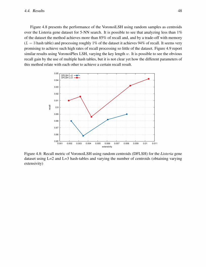
4.4. Results 48
Figure 4.8 presents the performance of the VoronoiLSH using random samples as centroidsover the Listeria gene dataset for 5-NN search. It is possible to see that analyzing less than 1%of the dataset the method achieves more than 85% of recall and, and by a trade-off with memory(L = 3 hash table) and processing roughly 1% of the dataset it achieves 94% of recall. It seems verypromising to achieve such high rates of recall processing so little of the dataset. Figure 4.9 reportsimilar results using VoronoiPlex LSH, varying the key length w. It is possible to see the obviousrecall gain by the use of multiple hash tables, but it is not clear yet how the different parameters ofthis method relate with each other to achieve a certain recall result.
0.85
0.86
0.87
0.88
0.89
0.9
0.91
0.92
0.93
0.94
0.95
0.001 0.002 0.003 0.004 0.005 0.006 0.007 0.008 0.009 0.01 0.011
recall
extensivity
DFLSH L=2DFLSH L=3
Figure 4.8: Recall metric of VoronoiLSH using random centroids (DFLSH) for the Listeria genedataset using L=2 and L=3 hash-tables and varying the number of centroids (obtaining varyingextensivity)

4.4. Results 49
0.00 0.05 0.10 0.15 0.20 0.25
extensivity
0.55
0.60
0.65
0.70
0.75
0.80
0.85
0.90
0.95
1.00
reca
ll
w=2
w=5
w=10
W=2W=5
W=10
VoronoiPlex LSH for L=1,nCluster=10
VoronoiPlex LSH for L=8,nCluster=10
Figure 4.9: Recall metric of VoronoiPlex LSH using random centroids (10 centroids selected from a4000 point sample set) for the Listeria gene dataset using L=1 and L=8 hash-tables and varying thesize w of the key-length
4.4.4 BigANN Dataset: Large-Scale Distributed Voronoi LSH
The large-scale evaluation used a distributed-memory machine with 70 nodes interconnectedthrough a FDR Infiniband switch. Each computation node was equipped with a dual-socket Intel E52.60 GHz Sandy Bridge processor with a total of 16 CPU cores, 32 GB of DDR3 RAM, runningLinux OS kernel version 2.6.32. Parallel Voronoi LSH was implemented on C++ and MPI.
Figure 4.10: Random seeds vs. K-means++ centroids on Parallel Voronoi LSH (BigAnn). Well-chosen seeds have little effect on recall, but occasionally lower query times.
The Figure 4.10 shows the query phase execution time and recall of parallel Voronoi LSHusing BigANN dataset with Voronoi seeds chosen at random, and by using K-means++ centroids.Although the difference in recall is negligible, using K-means++ centroids in general resulted in

4.4. Results 50
better query times than using random seeds. The best execution time in both cases was with 10,000Voronoi seeds. For minimizing the distance computations, there is an expected compromise betweentoo few seeds (cheap hash functions, large shortlists due to more points in buckets) and too many(costly hash functions, smaller shortlists). The theoretical sweet spot is obtained with
√n seeds,
where n is the dataset size (around 30,000 for BigAnn). However, in our tests, the empirical bestvalue was always much smaller than that, favoring, thus, the retrieval of fewer buckets with manypoints in them, instead of many buckets with fewer points. That suggests that the cost of accessingthe data is overcoming the cost of computing the distances.
Our parallelism efficiency analysis employs a scale-up (weak scaling) experiment in whichthe reference dataset and the number of computing cores used increase proportionally. A scale-upevaluation was selected because we expect to obtain an abundant volume of data for indexing, whichwould only fit in a distributed system. For each CPU core allocated to the BI stage 4 CPU cores areassigned to the DP stage, resulting in a ratio of computing cores by BI:DP of 1:4. A single core isused for the AG stage.
Figure 4.11: Efficiency of Parallel Voronoi LSH parallelization as the number of nodes used andthe reference dataset size increase proportionally. The results show that the parallelism schemescales-up well even for a very large dataset, with modest overhead.
The efficiency of the parallel Voronoi LSH is presented in Figure 4.11. As the number ofCPU cores and nodes used increase, the application achieves a very good parallel efficiencyof 0.9 when 801 computing cores are used (10 nodes for BI and 40 nodes for DP), indicatingvery modest parallelism overheads. The high efficiency attained is a result of (i) the applicationasynchronous design that decouples communication from computation tasks and of (ii) the intra-stage parallelization that allows for a single multi-threaded copy of the DP stage to be instantiatedper computing node. As a consequence, a smaller number of partitions of the reference dataset arecreated, which reduces the number of messages exchanged by the parallel version (using 51 nodes)in more than 6× as compared to an application version that instantiates a single process per CPUcomputing core.

Chapter 5
Conclusion
Efficient large-scale similarity search is a crucial operation for Content-based Multimedia Infor-mation Retrieval (CMIR) systems. But because those systems employ high-dimensional featurevectors, or other complex representations in metric spaces, providing fast similarity search forthem has been a persistent research challenge. LSH, a very successful family of methods, has beenadvanced as a solution to the problem, but it is available only for a few distance functions.
Voronoi diagrams has been long established as one of the top method for solving nearest-neighbor queries in two dimensional Euclidean spaces. However, difficult to generalize due to thenecessity of an exponential amount of space to maintain the polygons that represent the Voronoiregion. Nevertheless there has been a variety of methods in high-dimensional Euclidean spaces usingK-Means (or other Vector Quantization methods) for Nearest-Neighbor queries, and after someanalysis, it is possible to see the k-means partitioning and Vector Quantization as a form of Voronoipartitioning of the data, but dropping the need to store the partition polygons, maintaining only acentral element as a representative of the partition. We pursue this same idea for general metricspace and use it to address the limitation of possible distance and space for hashing, by extendingLSH to general metric spaces, using a Voronoi diagram as basis for a LSH family of functionsusing “central” points to represent the partitioning. We have proposed a method that follows amore directly the application of this general idea of partitioning (VoronoiLSH) and another onethat builds up on this idea in order to create a more selective hash (VoronoiPlex LSH). The centraltheoretical development is a proof that VoronoiLSH is (r, cr, p1, p2)-locality sensitive hashing familyunder some limited assumptions and that the average performance of the method is sub-linear. Theextension of the analysis for VoronoiPlex is natural and is similar to the concatenation “trick” usedon the original formulation of LSH, nevertheless a follow-up work should be done in order to beobtained a more complete theoretical characterization of VoronoiPlex. In the algorithm design,to avoid repetitive distance calculations, we added a structure maintained the index of the pointsselected for a group of hash functions and also presented results characterizing the expected numberof points shared by the group of hash functions – it remains open to investigation how this additionalstructure can affect the final quality.
Our experiments show our partitioning strategy to index the data works well both for metric and
51

5.1. Open questions and future work 52
for Euclidean data. The experiments do not show any clear advantage in learning the seeds of theVoronoi diagram by clustering: a random choice seems to work just as well. Further experimentalevaluation and theoretical analysis should be pursued in order to confirm or discard the advantagesof learning the centroids. If learning does not play a key role in quality of the search, it will alsobe an important hint for scalability, since clustering is expensive. On the other hand, clusteringmight in some cases affect query times, which is surprising. This seems to be due to a more uniformpartition of the data, since random seeds tend to create an unbalanced distribution of the dataset onthe buckets of the hash tables. The large-scale experiments show that our proposed parallelizationhas very modest overhead and scales-up well even for a very large collection.
5.1 Open questions and future work
This work is certainly not exhaustive and there is many opened doors to pursue. One of the morecentral problems is related to the probabilistic bounds of the hashing methods. The question ishow can we integrate our analysis, with other in the similarity metric space framework that usesconcentration of measures [Pestov, 2000, 2008; Volnyansky and Pestov, 2009] and unveil the roleof intrinsic dimensionality in the case of hashing-based methods for metric indexing, following,for example, interesting relationship between intrinsic dimensionality and discriminability [Houle,2013]. Another possible fruitful direction would be to follow recent developments in the area ofPtolemaic Indexing, which assumes a more specific inequality axiom (more specific compared tothe triangle inequality), and analyze how the proposed methods would work under those differentassumptions and design possible adaptations of the method for this different setup.
5.2 Concluding Remarks
This work present two randomized hashing methods designed to approach the problem of similaritysearch in general metric spaces: VoronoiLSH and VoronoiPlex LSH. Those methods are naturalextension to the metric space framework of the established Locality-Sensitive Hashing designed forHamming, Vector (Angular) and Euclidean Spaces. We offered theoretical characterization of themethods using limiting bounds on the hashing collision probabilities, and average case performanceof the search algorithms. Experimental validation and performance comparison with other methodsin the literature were presented and the results are good.
We developed, in a collaboration work, a parallelization of the VoronoiLSH algorithms andperformed weak scaling experiments on the a thousand million high dimensional points dataset andconclude that the parallel algorithm presented very modest parallelization overhead.
All evidences suggest that using metric partitioning techniques for designing hashing functionsfor metric space is an effective technique and should be further explored and developed.
We reported to the community two of these results: an initial article presenting VoronoiLSH ina national event (SBBD 2013) and an article describing the parallelization of VoronoiLSH to bepresented in an international event (SISAP 2014):

5.2. Concluding Remarks 53
• Eliezer Silva, Thiago Teixeira, George Teodoro, and Eduardo Valle. Large-scale distributedlocality-sensitive hashing for general metric data. In Similarity Search and Applications- Proceedings of the 7th International Conference on Similarity Search and Applications.Springer, October 2014
• Eliezer Silva and Eduardo Valle. K-medoids lsh: a new locality sensitive hashing in generalmetric space. In Proceedings of the 28th Brazilian Symposium on Databases, pages 127–132, Brazil, 2013. SBC. URL http://sbbd2013.cin.ufpe.br/Proceedings/
artigos/sbbd_shp_22.html

Bibliography
Charu C. Aggarwal, Alexander Hinneburg, and DanielA. Keim. On the surprising behaviorof distance metrics in high dimensional space. In Jan Van den Bussche and Victor Vianu,editors, Database Theory — ICDT 2001, volume 1973 of Lecture Notes in Computer Science,pages 420–434. Springer Berlin Heidelberg, 2001. ISBN 978-3-540-41456-8. doi: 10.1007/3-540-44503-X 27. URL http://dx.doi.org/10.1007/3-540-44503-X_27.
Giuseppe Amato and Pasquale Savino. Approximate similarity search in metric spaces using invertedfiles. In Proceedings of the 3rd International Conference on Scalable Information Systems,InfoScale ’08, pages 28:1–28:10, ICST, Brussels, Belgium, Belgium, 2008. ICST (Institute forComputer Sciences, Social-Informatics and Telecommunications Engineering). ISBN 978-963-9799-28-8. URL http://dl.acm.org/citation.cfm?id=1459693.1459731.
Alexandr Andoni. Nearest neighbor search: the old, the new, and the impossible. PhD thesis,Massachusetts Institute of Technology, 2009.
Alexandr Andoni and Piotr Indyk. Near-Optimal Hashing Algorithms for Approximate Near-est Neighbor in High Dimensions. In focs, pages 459–468. Ieee, 2006. ISBN 0-7695-2720-5. doi: 10.1109/FOCS.2006.49. URL http://ieeexplore.ieee.org/lpdocs/
epic03/wrapper.htm?arnumber=4031381.
Alexandr Andoni, Piotr Indyk, Huy L. Nguyen, and Ilya Razenshteyn. Beyond locality-sensitivehashing. In Chandra Chekuri, editor, SODA, pages 1018–1028. SIAM, 2014. ISBN 978-1-61197-338-9, 978-1-61197-340-2.
Remzi H. Arpaci-Dusseau, Eric Anderson, Noah Treuhaft, David E. Culler, Joseph M. Hellerstein,David A. Patterson, and Katherine Yelick. Cluster I/O with River: Making the Fast Case Common.In IOPADS ’99: Input/Output for Parallel and Distributed Systems, Atlanta, GA, May 1999.
David Arthur and Sergei Vassilvitskii. k-means++: the advantages of careful seeding. In Proceedingsof the eighteenth annual ACM-SIAM symposium on Discrete algorithms, SODA ’07, pages 1027–1035, Philadelphia, PA, USA, 2007. Society for Industrial and Applied Mathematics. ISBN 978-0-898716-24-5. URL http://dl.acm.org/citation.cfm?id=1283383.1283494.
Michal Batko. Scalable and Distributed Similarity Search. PhD thesis, Masarykova univerzita,Fakulta informatiky, 2006. URL <http://is.muni.cz/th/2907/fi_d/>.
54

BIBLIOGRAPHY 55
Mayank Bawa, Tyson Condie, and Prasanna Ganesan. LSH forest. In Proceedings ofthe 14th international conference on World Wide Web - WWW ’05, page 651, NewYork, New York, USA, 2005. ACM Press. ISBN 1595930469. doi: 10.1145/1060745.1060840. URL http://dl.acm.org/citation.cfm?id=1060840http:
//portal.acm.org/citation.cfm?doid=1060745.1060840.
Richard Ernest Bellman. Adaptive control processes: a guided tour, volume 4 of ’Rand Corporation.Research studies. Princeton University Press, 1961.
Kevin S. Beyer, Jonathan Goldstein, Raghu Ramakrishnan, and Uri Shaft. When is ”nearestneighbor” meaningful? In Proceedings of the 7th International Conference on Database Theory,ICDT ’99, pages 217–235, London, UK, UK, 1999. Springer-Verlag. ISBN 3-540-65452-6. URLhttp://dl.acm.org/citation.cfm?id=645503.656271.
Michael D. Beynon, Tahsin Kurc, Umit Catalyurek, Chialin Chang, Alan Sussman, and JoelSaltz. Distributed processing of very large datasets with DataCutter. Parallel Comput., 27(11):1457–1478, 2001. ISSN 0167-8191. doi: http://dx.doi.org/10.1016/S0167-8191(01)00099-0.
J. Bourgain. On lipschitz embedding of finite metric spaces in hilbert space. Israel Journalof Mathematics, 52(1-2):46–52, 1985. ISSN 0021-2172. doi: 10.1007/BF02776078. URLhttp://dx.doi.org/10.1007/BF02776078.
Andrei Z Broder, Moses Charikar, Alan M Frieze, and Michael Mitzenmacher. Min-wise indepen-dent permutations. Journal of Computer and System Sciences, 60(3):630–659, 2000.
W. A. Burkhard and R. M. Keller. Some approaches to best-match file searching. Commun.ACM, 16(4):230–236, April 1973. ISSN 0001-0782. doi: 10.1145/362003.362025. URLhttp://doi.acm.org/10.1145/362003.362025.
Moses S Charikar. Similarity estimation techniques from rounding algorithms. In Proceedings ofthe thiry-fourth annual ACM symposium on Theory of computing, pages 380–388. ACM, 2002.
Edgar Chavez and Gonzalo Navarro. A compact space decomposition for effective metric indexing.Pattern Recognition Letters, 26(9):1363–1376, 2005.
Edgar Chavez, Gonzalo Navarro, Ricardo Baeza-Yates, and Jose Luis Marroquın. Searching inmetric spaces. ACM Computing Surveys, 33(3):273–321, September 2001. ISSN 03600300.doi: 10.1145/502807.502808. URL http://portal.acm.org/citation.cfm?doid=
502807.502808.
Edgar Chavez, Karina Figueroa, and Gonzalo Navarro. Proximity searching in high dimensionalspaces with a proximity preserving order. In Alexander Gelbukh, Alvaro de Albornoz, and HugoTerashima-Marın, editors, MICAI 2005: Advances in Artificial Intelligence, volume 3789 ofLecture Notes in Computer Science, pages 405–414. Springer Berlin Heidelberg, 2005. ISBN

BIBLIOGRAPHY 56
978-3-540-29896-0. doi: 10.1007/11579427 41. URL http://dx.doi.org/10.1007/
11579427_41.
Paolo Ciaccia, Marco Patella, and Pavel Zezula. M-tree: An efficient access method for similaritysearch in metric spaces. In Proceedings of the 23rd International Conference on Very LargeData Bases, VLDB ’97, pages 426–435, San Francisco, CA, USA, 1997. Morgan KaufmannPublishers Inc. ISBN 1-55860-470-7. URL http://dl.acm.org/citation.cfm?id=
645923.671005.
Kenneth L Clarkson. Nearest-Neighbor Searching and Metric Space Dimensions. In Gre-gory Shakhnarovich, Trevor Darrell, and Piotr Indyk, editors, Nearest-Neighbor Methods inLearning and Vision: Theory and Practice (Neural Information Processing), Advances inNeural Information Processing Systems. The MIT Press, 2006. ISBN 026219547X. URLhttp://books.google.com.br/books?id=5FIZAQAAIAAJ.
Mayur Datar, Nicole Immorlica, Piotr Indyk, and Vahab S. Mirrokni. Locality-sensitive hashingscheme based on p-stable distributions. In Proceedings of the twentieth annual symposiumon Computational geometry - SCG ’04, page 253, New York, New York, USA, 2004. ACMPress. ISBN 1581138857. doi: 10.1145/997817.997857. URL http://portal.acm.org/
citation.cfm?doid=997817.997857.
Ritendra Datta, Dhiraj Joshi, Jia Li, and James Z. Wang. Image retrieval. ACM ComputingSurveys, 40(2):1–60, April 2008. ISSN 03600300. doi: 10.1145/1348246.1348248. URLhttp://portal.acm.org/citation.cfm?doid=1348246.1348248.
M Deza and M Laurent. Geometry of cuts and metrics. Algorithms and Combinatorics, 15:1–587,1997.
Michel Marie Deza and Elena Deza. Encyclopedia of distances. Springer, 2009.
David L Donoho et al. High-dimensional data analysis: The curses and blessings of dimensionality.AMS Math Challenges Lecture, pages 1–32, 2000.
K. Figueroa, G. Navarro, and E. Chavez. Metric spaces library, 2007. Available athttp://www.sisap.org/Metric Space Library.html .
A Flexer and D. Schnitzer. Can shared nearest neighbors reduce hubness in high-dimensionalspaces? In Data Mining Workshops (ICDMW), 2013 IEEE 13th International Conference on,pages 460–467, Dec 2013. doi: 10.1109/ICDMW.2013.101.
Kimmo Fredriksson. Engineering efficient metric indexes. Pattern Recognition Letters, 28(1):75–84, 2007.
Aristides Gionis, Piotr Indyk, and Rajeev Motwani. Similarity search in high dimensions viahashing. In Proceedings of the 25th International Conference on Very Large Data Bases, VLDB

BIBLIOGRAPHY 57
’99, pages 518–529, San Francisco, CA, USA, 1999. Morgan Kaufmann Publishers Inc. ISBN1-55860-615-7. URL http://dl.acm.org/citation.cfm?id=645925.671516.
Edgar Chavez Gonzalez, Karina Figueroa, and Gonzalo Navarro. Effective proximity retrieval byordering permutations. Pattern Analysis and Machine Intelligence, IEEE Transactions on, 30(9):1647–1658, 2008.
Magnus Lie Hetland. The basic principles of metric indexing. In Swarm intelligence for multi-objective problems in data mining, pages 199–232. Springer Berlin Heidelberg, 2009.
Gisli R. Hjaltason and Hanan Samet. Index-driven similarity search in metric spaces (surveyarticle). ACM Trans. Database Syst., 28(4):517–580, December 2003. ISSN 0362-5915. doi:10.1145/958942.958948. URL http://doi.acm.org/10.1145/958942.958948.
Michael E Houle. Dimensionality, discriminability, density and distance distributions. In DataMining Workshops (ICDMW), 2013 IEEE 13th International Conference on, pages 468–473.IEEE, 2013.
Piotr Indyk and Rajeev Motwani. Approximate nearest neighbors. In Proceedings of the thir-tieth annual ACM symposium on Theory of computing - STOC ’98, pages 604–613, NewYork, New York, USA, 1998. ACM Press. ISBN 0897919629. doi: 10.1145/276698.276876. URL http://dl.acm.org/citation.cfm?id=276876http://portal.
acm.org/citation.cfm?doid=276698.276876.
Herve Jegou, Laurent Amsaleg, Cordelia Schmid, and Patrick Gros. Query adaptative localitysensitive hashing. In 2008 IEEE International Conference on Acoustics, Speech and SignalProcessing, pages 825–828. IEEE, March 2008. ISBN 978-1-4244-1483-3. doi: 10.1109/ICASSP.2008.4517737. URL http://ieeexplore.ieee.org/lpdocs/epic03/wrapper.
htm?arnumber=4517737.
Herve Jegou, Romain Tavenard, Matthijs Douze, and Laurent Amsaleg. Searching in one billionvectors: Re-rank with source coding. In ICASSP, pages 861–864. IEEE, 2011. ISBN 978-1-4577-0539-7.
Alexis Joly and Olivier Buisson. A posteriori multi-probe locality sensitive hashing. In Proceedingsof the 16th ACM International Conference on Multimedia, MM ’08, pages 209–218, New York,NY, USA, 2008. ACM. ISBN 978-1-60558-303-7. doi: 10.1145/1459359.1459388. URLhttp://doi.acm.org/10.1145/1459359.1459388.
Byungkon Kang and Kyomin Jung. Robust and Efficient Locality Sensitive Hashing for NearestNeighbor Search in Large Data Sets. In NIPS Workshop on Big Learning (BigLearn), pages1–8, Lake Tahoe, Nevada, 2012. URL http://biglearn.org/2012/files/papers/
biglearning2012_submission_5.pdf.

BIBLIOGRAPHY 58
Leonard Kaufman and Peter J. Rousseeuw. Finding Groups in Data: An Introductionto Cluster Analysis. Wiley-Interscience, New York, USA, 9th edition, March 1990.ISBN 0471878766. URL http://www.amazon.com/exec/obidos/redirect?tag=citeulike07-20&path=ASIN/0471878766.
John Leech. Some sphere packings in higher space. Canadian Journal of Mathematics, 16:657–682, January 1964. ISSN 1496-4279. doi: 10.4153/CJM-1964-065-1. URL http:
//www.cms.math.ca/10.4153/CJM-1964-065-1.
David G. Lowe. Distinctive Image Features from Scale-Invariant Keypoints. International Journalof Computer Vision, 60(2):91–110, November 2004. ISSN 0920-5691. doi: 10.1023/B:VISI.0000029664.99615.94. URL http://www.springerlink.com/openurl.asp?id=
doi:10.1023/B:VISI.0000029664.99615.94.
Qin Lv, William Josephson, Zhe Wang, Moses Charikar, and Kai Li. Multi-probe LSH: efficientindexing for high-dimensional similarity search. In Proceedings of the 33rd internationalconference on Very large data bases, VLDB ’07, pages 950–961. VLDB Endowment, 2007.ISBN 978-1-59593-649-3. URL http://dl.acm.org/citation.cfm?id=1325851.
1325958.
Jirı Matousek. Lectures on discrete geometry, volume 108. Springer New York, 2002.
Jirı Matousek. On the distortion required for embedding finite metric spaces into normed spaces. Is-rael Journal of Mathematics, 93(1):333–344, 1996. ISSN 0021-2172. doi: 10.1007/BF02761110.URL http://dx.doi.org/10.1007/BF02761110.
Rajeev Motwani, Assaf Naor, and Rina Panigrahy. Lower bounds on locality sensitive hashing. InProceedings of the twenty-second annual symposium on Computational geometry - SCG ’06,page 154, New York, New York, USA, 2006. ACM Press. ISBN 1595933409. doi: 10.1145/1137856.1137881. URL http://portal.acm.org/citation.cfm?doid=1137856.
1137881.
RT Ng. CLARANS: a method for clustering objects for spatial data mining. IEEETransactions on Knowledge and Data Engineering, 14(5):1003–1016, Septem-ber 2002. ISSN 1041-4347. doi: 10.1109/TKDE.2002.1033770. URL http:
//ieeexplore.ieee.org/xpls/abs_all.jsp?arnumber=1033770http://
ieeexplore.ieee.org/lpdocs/epic03/wrapper.htm?arnumber=1033770.
David Novak and Michal Batko. Metric Index: An Efficient and Scalable Solution for SimilaritySearch. In 2009 Second International Workshop on Similarity Search and Applications, pages65–73. IEEE Computer Society, August 2009. ISBN 978-0-7695-3765-8. doi: 10.1109/SISAP.2009.26. URL http://ieeexplore.ieee.org/lpdocs/epic03/wrapper.htm?
arnumber=5272384.
BIBLIOGRAPHY 59
David Novak, Martin Kyselak, and Pavel Zezula. On locality-sensitive indexing in genericmetric spaces. In Proceedings of the Third International Conference on SImilarity Searchand APplications - SISAP ’10, pages 59–66, New York, New York, USA, 2010. ACM Press.ISBN 9781450304207. doi: 10.1145/1862344.1862354. URL http://portal.acm.org/
citation.cfm?doid=1862344.1862354.
Alexander Ocsa and Elaine P M De Sousa. An Adaptive Multi-level Hashing Structure for FastApproximate Similarity Search. Journal of Information and Data Management, 1(3):359–374,2010.
Ryan O’Donnell, Yi Wu, and Yuan Zhou. Optimal lower bounds for locality-sensitive hashing(except when q is tiny). ACM Trans. Comput. Theory, 6(1):5:1–5:13, March 2014. ISSN1942-3454. doi: 10.1145/2578221. URL http://doi.acm.org/10.1145/2578221.
Rafail Ostrovsky, Yuval Rabani, Leonard Schulman, and Chaitanya Swamy. The Effec-tiveness of Lloyd-Type Methods for the k-Means Problem. In focs, pages 165–176.IEEE, December 2006. ISBN 0-7695-2720-5. doi: 10.1109/FOCS.2006.75. URLhttp://dl.acm.org/citation.cfm?doid=2395116.2395117http://
ieeexplore.ieee.org/lpdocs/epic03/wrapper.htm?arnumber=4031353.
Rina Panigrahy. Entropy based nearest neighbor search in high dimensions. In Proceedings of theseventeenth annual ACM-SIAM symposium on Discrete algorithm, SODA ’06, pages 1186–1195,New York, NY, USA, 2006. ACM. ISBN 0-89871-605-5. doi: 10.1145/1109557.1109688. URLhttp://doi.acm.org/10.1145/1109557.1109688.
Hae-Sang Park and Chi-Hyuck Jun. A simple and fast algorithm for K-medoids cluster-ing. Expert Systems with Applications, 36(2):3336–3341, 2009. ISSN 09574174. doi:10.1016/j.eswa.2008.01.039. URL http://linkinghub.elsevier.com/retrieve/
pii/S095741740800081X.
Marco Patella and Paolo Ciaccia. Approximate similarity search: A multi-faceted problem.Journal of Discrete Algorithms, 7(1):36 – 48, 2009. ISSN 1570-8667. doi: http://dx.doi.org/10.1016/j.jda.2008.09.014. URL http://www.sciencedirect.com/science/
article/pii/S1570866708000762. Selected papers from the 1st International Work-shop on Similarity Search and Applications (SISAP) 1st International Workshop on SimilaritySearch and Applications (SISAP).
Adriano Arantes Paterlini, Mario A Nascimento, and Caetano Traina Junior. Using Pivots to Speed-Up k-Medoids Clustering. Journal of Information and Data Management, 2(2):221–236, June2011. URL http://seer.lcc.ufmg.br/index.php/jidm/article/view/99.
Loıc Pauleve, Herve Jegou, and Laurent Amsaleg. Locality sensitive hashing: A comparisonof hash function types and querying mechanisms. Pattern Recognition Letters, 31(11):1348–1358, August 2010. ISSN 01678655. doi: 10.1016/j.patrec.2010.04.004. URL http://
linkinghub.elsevier.com/retrieve/pii/S0167865510001169.

BIBLIOGRAPHY 60
Vladimir Pestov. On the geometry of similarity search: Dimensionality curse and concentrationof measure. Information Processing Letters, 73(1–2):47 – 51, 2000. ISSN 0020-0190. doi:http://dx.doi.org/10.1016/S0020-0190(99)00156-8. URL http://www.sciencedirect.
com/science/article/pii/S0020019099001568.
Vladimir Pestov. An axiomatic approach to intrinsic dimension of a dataset. Neural Networks, 21(2):204–213, 2008.
Milos Radovanovic, Alexandros Nanopoulos, and Mirjana Ivanovic. Nearest neighbors in high-dimensional data: The emergence and influence of hubs. In Proceedings of the 26th AnnualInternational Conference on Machine Learning, ICML ’09, pages 865–872, New York, NY,USA, 2009. ACM. ISBN 978-1-60558-516-1. doi: 10.1145/1553374.1553485. URL http:
//doi.acm.org/10.1145/1553374.1553485.
Milos Radovanovic, Alexandros Nanopoulos, and Mirjana Ivanovic. Hubs in space: Popular nearestneighbors in high-dimensional data. J. Mach. Learn. Res., 11:2487–2531, December 2010. ISSN1532-4435. URL http://dl.acm.org/citation.cfm?id=1756006.1953015.
Satish Rao. Small distortion and volume preserving embeddings for planar and euclidean metrics.In Proceedings of the fifteenth annual symposium on Computational geometry, pages 300–306.ACM, 1999.
Hanan Samet. Foundations of Multidimensional and Metric Data Structures. Morgan KaufmannPublishers Inc., San Francisco, CA, USA, 2005. ISBN 0123694469.
Uri Shaft and Raghu Ramakrishnan. Theory of nearest neighbors indexability. ACM Trans. DatabaseSyst., 31(3):814–838, September 2006. ISSN 0362-5915. doi: 10.1145/1166074.1166077. URLhttp://doi.acm.org/10.1145/1166074.1166077.
Eliezer Silva and Eduardo Valle. K-medoids lsh: a new locality sensitive hashing in gen-eral metric space. In Proceedings of the 28th Brazilian Symposium on Databases, pages127–132, Brazil, 2013. SBC. URL http://sbbd2013.cin.ufpe.br/Proceedings/
artigos/sbbd_shp_22.html.
Eliezer Silva, Thiago Teixeira, George Teodoro, and Eduardo Valle. Large-scale distributed locality-sensitive hashing for general metric data. In Similarity Search and Applications - Proceedings ofthe 7th International Conference on Similarity Search and Applications. Springer, October 2014.
Tomas Skopal. Where are you heading, metric access methods?: a provocative survey. In Pro-ceedings of the Third International Conference on SImilarity Search and APplications, SISAP’10, pages 13–21, New York, NY, USA, 2010. ACM. ISBN 978-1-4503-0420-7. doi: 10.1145/1862344.1862347. URL http://doi.acm.org/10.1145/1862344.1862347.
Malcolm Slaney, Yury Lifshits, and Junfeng He. Optimal Parameters for Locality-Sensitive Hashing.Proceedings of the IEEE, 100(9):2604–2623, 2012.

BIBLIOGRAPHY 61
Eric Sadit Tellez and Edgar Chavez. On locality sensitive hashing in metric spaces. In Proceedings ofthe Third International Conference on SImilarity Search and APplications, SISAP ’10, pages 67–74, New York, NY, USA, 2010. ACM. ISBN 978-1-4503-0420-7. doi: 10.1145/1862344.1862355.URL http://doi.acm.org/10.1145/1862344.1862355.
George Teodoro, Daniel Fireman, Dorgival Guedes, Wagner Meira Jr., and Renato Ferreira.Achieving multi-level parallelism in the filter-labeled stream programming model. Paral-lel Processing, International Conference on, 0:287–294, 2008. ISSN 0190-3918. doi:http://doi.ieeecomputersociety.org/10.1109/ICPP.2008.72.
A.J.M. Traina, A. Traina, C. Faloutsos, and B. Seeger. Fast indexing and visualization of metric datasets using slim-trees. Knowledge and Data Engineering, IEEE Transactions on, 14(2):244–260,2002. ISSN 1041-4347. doi: 10.1109/69.991715.
Caetano Traina, Jr., Agma J. M. Traina, Bernhard Seeger, and Christos Faloutsos. Slim-trees:High performance metric trees minimizing overlap between nodes. In Proceedings of the 7thInternational Conference on Extending Database Technology: Advances in Database Technology,EDBT ’00, pages 51–65, London, UK, UK, 2000. Springer-Verlag. ISBN 3-540-67227-3. URLhttp://dl.acm.org/citation.cfm?id=645339.650146.
Jeffrey K. Uhlmann. Satisfying general proximity / similarity queries with metric trees. Infor-mation Processing Letters, 40(4):175 – 179, 1991. ISSN 0020-0190. doi: http://dx.doi.org/10.1016/0020-0190(91)90074-R. URL http://www.sciencedirect.com/science/
article/pii/002001909190074R.
Ilya Volnyansky and Vladimir Pestov. Curse of dimensionality in pivot based indexes. In Proceed-ings of the 2009 Second International Workshop on Similarity Search and Applications, pages39–46. IEEE Computer Society, 2009.
Peter N. Yianilos. Data structures and algorithms for nearest neighbor search in general metricspaces. In Proceedings of the fourth annual ACM-SIAM Symposium on Discrete algorithms,SODA ’93, pages 311–321, Philadelphia, PA, USA, 1993. Society for Industrial and AppliedMathematics. ISBN 0-89871-313-7. URL http://dl.acm.org/citation.cfm?id=
313559.313789.
Pavel Zezula. Future trends in similarity searching. In Proceedings of the 5th internationalconference on Similarity Search and Applications, SISAP’12, pages 8–24, Berlin, Heidelberg,2012. Springer-Verlag. ISBN 978-3-642-32152-8. doi: 10.1007/978-3-642-32153-5 2. URLhttp://dx.doi.org/10.1007/978-3-642-32153-5_2.
Pavel Zezula, Giuseppe Amato, Vlastislav Dohnal, and Michal Batko. Similarity Search - TheMetric Space Approach, volume 32 of Advances in Database Systems. Kluwer AcademicPublishers, Boston, 2006. ISBN 0-387-29146-6. doi: 10.1007/0-387-29151-2. URL http:
//www.springerlink.com/index/10.1007/0-387-29151-2.

BIBLIOGRAPHY 62
Qiaoping Zhang and Isabelle Couloigner. A new and efficient k-medoid algorithm for spatialclustering. In Osvaldo Gervasi, MarinaL. Gavrilova, Vipin Kumar, Antonio Lagana, HeowPuehLee, Youngsong Mun, David Taniar, and ChihJengKenneth Tan, editors, Computational Scienceand Its Applications (ICCSA), volume 3482 of Lecture Notes in Computer Science, pages 181–189. Springer Berlin Heidelberg, Singapore, 2005. ISBN 978-3-540-25862-9. doi: 10.1007/11424857 20. URL http://dx.doi.org/10.1007/11424857_20.

Appendix A
Implementation
63

64
Figu
reA
.1:C
lass
diag
ram
ofth
esy
stem