ELF/VLF wave generation using simultaneous CW and modulatedHF heating of the ionosphere

R. C. Moore1 and D. Agrawal1

Received 2 July 2010; revised 11 January 2011; accepted 14 January 2011; published 19 April 2011.

[1] Experimental observations of ELF/VLF waves generated using the dual‐beam heatingcapability of the High frequency Active Auroral Research Program (HAARP) HFtransmitter in Gakona, Alaska, are compared with the predictions of an ionospheric HFheating model that accounts for the simultaneous propagation and absorption of multipleHF beams. The model output is used to assess three properties of the ELF/VLF wavesobserved on the ground: the ELF/VLF signal magnitude, the ELF/VLF harmonic ratio,and the ELF/VLF power law exponent. Ground‐based experimental observations indicatethat simultaneous heating of the ionosphere by a CW HF wave and a modulated HFwave generates significantly lower ELF/VLF magnitudes than during periods without CWheating, consistent with model predictions. Further modeling predictions demonstratethe sensitive dependence of ELF/VLF magnitude on the frequency and power of theCW signal. The ratio of ELF/VLF harmonic magnitudes is also shown to be a sensitiveindicator of ionospheric modification, although it is somewhat less sensitive than theELF/VLF magnitude. Last, the peak power level of the modulated HF beam was variedin order to assess the power dependence of ELF/VLF wave generation under both single‐and dual‐beam heating conditions. Experimental and theoretical results indicate thataccurate evaluation of the ELF/VLF power law index requires high signal‐to‐noise ratio;it is thus a less sensitive indicator of ionospheric modification than either ELF/VLFmagnitude or the ELF/VLF harmonic ratio.

Citation: Moore, R. C., and D. Agrawal (2011), ELF/VLF wave generation using simultaneous CW and modulated HF heatingof the ionosphere, J. Geophys. Res., 116, A04217, doi:10.1029/2010JA015902.

1. Introduction

[2] It is by now well known that modulated HF heating ofthe lower ionosphere in the presence of auroral electrojetcurrents can be used as an effective means for generatingelectromagnetic waves with frequencies varying from lessthan several hertz to greater than several kilohertz (i.e., theELF/VLF frequency band) [e.g., Getmantsev et al., 1974;Stubbe et al., 1982; Barr et al., 1991; Villaseñor et al.,1996; Papadopoulos et al., 2003; Moore et al., 2006;Cohen et al., 2010]. Recent experimental and theoreticalefforts have focused on methods to improve the efficiencyof ELF/VLF wave generation. For instance, Cohen et al.[2010] explored the use of a creative technique that mod-ulates the direction of the HF beam rather than the power ofthe HF beam to generate ELF/VLF waves, and Milikh andPapadopoulos [2007] theoretically analyzed the effect oflong periods of CW heating prior to modulated heating.Recent hardware upgrades at the High frequency ActiveAuroral Research Program (HAARP) HF transmitter in

Gakona, Alaska have provided an incredibly useful andversatile tool for probing and understanding the dynamicsof high‐power HF heating of the ionosphere. In particular,this paper will focus on the dual‐beam transmission capa-bility now available at HAARP to assess the veracity of amultiple‐beam ionospheric heating model, noting that themanipulation of multiple HF beams may possibly lead toan improvement in ELF/VLF wave generation efficiency inthe future.[3] In this paper, we compare numerical modeling pre-

dictions with experimental observations in order to validatea multiple‐beam ionospheric heating model. Each of thedual‐beam transmissions in this experiment use the combi-nation of a modulated HF wave and an unmodulated (CW)HF wave, including periods with the CW beam turned OFF(i.e., single‐beam heating). We compare the relative ELF/VLF magnitudes during CW‐ON and CW‐OFF periods andshow that the addition of a CW beam decreases the mag-nitude of the ELF/VLF wave observed on the ground. Weexplore this relationship theoretically as a function of thefrequency and power of the CW beam. We identify theharmonic ratio as an additional sensitive indicator of iono-spheric modification. Last, we demonstrate that although themagnitude of the ELF/VLF signal received on the grounddecreases under CW‐heated conditions, the rate of ELF/

1Department of Electrical and Computer Engineering, University ofFlorida, Gainesville, Florida, USA.

Copyright 2011 by the American Geophysical Union.0148‐0227/11/2010JA015902

JOURNAL OF GEOPHYSICAL RESEARCH, VOL. 116, A04217, doi:10.1029/2010JA015902, 2011

A04217 1 of 15

VLF magnitude change with the peak power of the modu-lated HF beam does not change significantly.

2. Description of the Experiment

[4] During a 30 min period between 0830 and 0900 UTon 2 August 2007, the 12 × 15 HAARP HF transmitter arraywas divided into two 6 × 15 subarrays, each with a peakpower of 1800 kW. One subarray was used to generate ELF/VLF waves in the ionosphere by transmitting a sinusoidalamplitude modulated (at 1215 Hz and 2430 Hz) beam at4.5 MHz (X mode polarization), stepping the peak HFpower in 15 distinct log‐based steps (from −12.5 dB to 0 dBwith 1 s at each power level). Simultaneously, the secondbeam of the HAARP HF transmitter continually heated thesame patch of ionosphere at peak power at 3.25 MHz (CW,X mode) for a period of 8 min. A lower HF frequency wasselected for the CW beam so that the CW beam patternwould be broader than that of the modulated 4.5 MHz HFbeam. The 8 min CW transmission block was followed by a7 min period without CW heating (that is, the first beamcontinued to modulate at 4.5 MHz while the second beamwas OFF). A cartoon depiction of the HF beam configura-tion can be seen in Figure 1, and a diagram of the mod-ulation frequency and HF power format can be seen inFigure 2. The gains of the two subarrays depend on thefrequencies transmitted. For the purposes of modeling, wehave approximated the peak effective radiated power (ERP)levels (using 6 × 15 subarrays) to be 78.9 dBW at 3.25 MHzand 84.2 dBW at 4.5 MHz. The 15 min experiment wasrepeated twice during the 30 min window, and the KP indexwas 2 at this time.[5] ELF/VLF wave observations were performed at a

ground‐based receiver located at the HAARP observatory,approximately 1.5 km from the HF transmitter. The radialand azimuthal components of the magnetic field weremonitored continually. The receiver is sensitive to magneticfields with frequencies between ∼500 Hz and ∼45 kHz. Datawere sampled at 100 kHz with 16‐bit resolution. In post-processing, the narrowband ELF/VLF amplitudes and pha-ses at the modulation frequencies and their harmonics weredetermined using 1 s long discrete Fourier transforms.

[6] The ELF/VLF receiver used at HAARP has beenrigorously tested to determine whether the observed ELF/VLF signals could be artificially created by nonlineardemodulation of the HF wave arriving at the receiver. If thiswere the case, one would expect to observe nonlinear effectson other ELF and VLF signals recorded in the data at thetime of transmission, and these effects are not observed. Forinstance, modulation sidebands are not observed on VLFtransmitter signals (in the 20–25 kHz range), and naturalVLF signals do not exhibit evidence of receiver saturationor other nonlinearities, despite the fact that these signals aretypically many times stronger than the ELF/VLF signalsgenerated by modulated heating of auroral electrojet cur-rents. Additionally, direct measurements of common‐modeand differential‐mode signal coupling also suggest that theobserved ELF/VLF signals are generated by modulatedheating of the auroral electrojet currents, rather than bynonlinear demodulation of the HF wave in the receiverelectronics. Injected common‐mode signals at 1.6 MHzwere reduced by 40 dB compared to signals at 1 kHz, andcommon‐mode signals at higher frequencies were too smallto be measured. Injected differential‐mode signals measuredat 1 MHz were reduced by 40 dB from the 1 kHz value.Higher‐frequency differential‐mode signals were also toosmall to measure accurately.

3. Experimental Observations

[7] Figure 3 shows the magnitude of the ELF/VLF signalobserved at HAARP at 1215 Hz and 2430 Hz for the entire

Figure 1. A cartoon diagram of the dual‐beam HF heatingexperiment. The 3.25 MHz CW beam is broader than the4.5 MHz modulated beam.

Figure 2. The transmission schedule for the 4.5 MHz mod-ulated HF beam. (top) The modulation frequency (sinusoidalAM) as a function of time. (bottom) The peak poweremployed as a function of time. A modulation depth of100% was used for all cases. Both panels share the same timeaxis. This 30 s schedule repeated continually for 30 min.

MOORE AND AGRAWAL: MODULATED AND CW HEATING A04217A04217

2 of 15

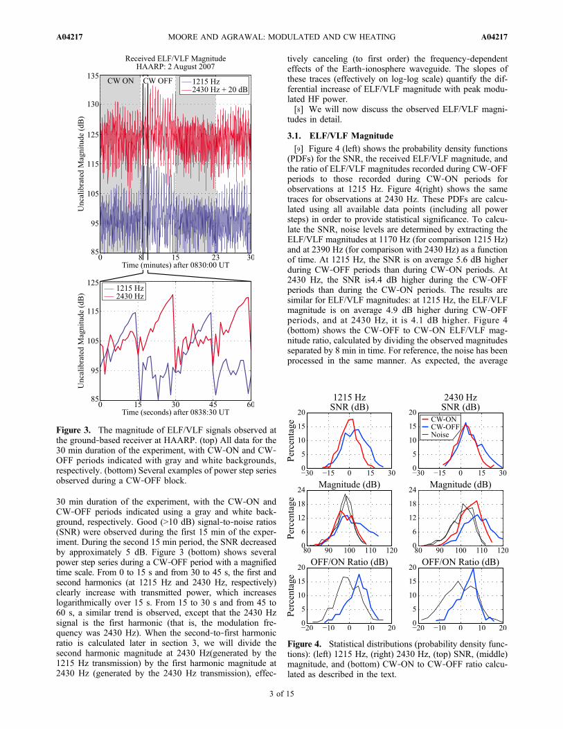
30 min duration of the experiment, with the CW‐ON andCW‐OFF periods indicated using a gray and white back-ground, respectively. Good (>10 dB) signal‐to‐noise ratios(SNR) were observed during the first 15 min of the exper-iment. During the second 15 min period, the SNR decreasedby approximately 5 dB. Figure 3 (bottom) shows severalpower step series during a CW‐OFF period with a magnifiedtime scale. From 0 to 15 s and from 30 to 45 s, the first andsecond harmonics (at 1215 Hz and 2430 Hz, respectively)clearly increase with transmitted power, which increaseslogarithmically over 15 s. From 15 to 30 s and from 45 to60 s, a similar trend is observed, except that the 2430 Hzsignal is the first harmonic (that is, the modulation fre-quency was 2430 Hz). When the second‐to‐first harmonicratio is calculated later in section 3, we will divide thesecond harmonic magnitude at 2430 Hz(generated by the1215 Hz transmission) by the first harmonic magnitude at2430 Hz (generated by the 2430 Hz transmission), effec-

tively canceling (to first order) the frequency‐dependenteffects of the Earth‐ionosphere waveguide. The slopes ofthese traces (effectively on log‐log scale) quantify the dif-ferential increase of ELF/VLF magnitude with peak modu-lated HF power.[8] We will now discuss the observed ELF/VLF magni-

tudes in detail.

3.1. ELF/VLF Magnitude

[9] Figure 4 (left) shows the probability density functions(PDFs) for the SNR, the received ELF/VLF magnitude, andthe ratio of ELF/VLF magnitudes recorded during CW‐OFFperiods to those recorded during CW‐ON periods forobservations at 1215 Hz. Figure 4(right) shows the sametraces for observations at 2430 Hz. These PDFs are calcu-lated using all available data points (including all powersteps) in order to provide statistical significance. To calcu-late the SNR, noise levels are determined by extracting theELF/VLF magnitudes at 1170 Hz (for comparison 1215 Hz)and at 2390 Hz (for comparison with 2430 Hz) as a functionof time. At 1215 Hz, the SNR is on average 5.6 dB higherduring CW‐OFF periods than during CW‐ON periods. At2430 Hz, the SNR is4.4 dB higher during the CW‐OFFperiods than during the CW‐ON periods. The results aresimilar for ELF/VLF magnitudes: at 1215 Hz, the ELF/VLFmagnitude is on average 4.9 dB higher during CW‐OFFperiods, and at 2430 Hz, it is 4.1 dB higher. Figure 4(bottom) shows the CW‐OFF to CW‐ON ELF/VLF mag-nitude ratio, calculated by dividing the observed magnitudesseparated by 8 min in time. For reference, the noise has beenprocessed in the same manner. As expected, the average

Figure 4. Statistical distributions (probability density func-tions): (left) 1215 Hz, (right) 2430 Hz, (top) SNR, (middle)magnitude, and (bottom) CW‐ON to CW‐OFF ratio calcu-lated as described in the text.

Figure 3. The magnitude of ELF/VLF signals observed atthe ground‐based receiver at HAARP. (top) All data for the30 min duration of the experiment, with CW‐ON and CW‐OFF periods indicated with gray and white backgrounds,respectively. (bottom) Several examples of power step seriesobserved during a CW‐OFF block.

MOORE AND AGRAWAL: MODULATED AND CW HEATING A04217A04217

3 of 15

results are similar: a 4.9 dB ratio is observed at 1215 Hz,and a 4.5 dB ratio is observed at 2430 Hz. The fact thatthese distributions are very similar to each other supports thestatement that the ELF/VLF magnitude is significantlyreduced by additional CW heating.[10] In order to assess the effects of CW heating on the

magnitude of the received ELF/VLF signal as a function oftime, we select the magnitude of the first harmonic at thepeak power transmission (i.e., the 15th power step). Thisselection supplies observations with the highest SNR. Thesemagnitudes are available once every 30 s, and they areshown in Figure 5 for both 1215 Hz and 2430 Hz. Themagnitudes exhibit a natural variation on the order of sev-eral dB over the 30 min experiment. This variation is likelydominated by the varying strength of the auroral electrojetcurrents, but also may be due to variations in electrondensity and electron temperature in the D region ionosphere.On the one hand, the variations in ionospheric parametersmay be produced directly by HF heating; on the other handthey may also occur naturally, produced, for instance, byenergetic electron precipitation or other natural phenomena.The observed change in ELF/VLF magnitude between CW‐ON and CW‐OFF periods, however, can be directly attrib-uted to HF heating. At 1215 Hz and 2430 Hz, the magni-tudes of the ELF/VLF signals increase by 8.6 and 8.1 dB,respectively, when the CW beam is turned off. The SNR atthis point in time was 16.6 dB at1225 Hz and 22.2 dB at2130 Hz. When the CW beam is turned on again 7 min later,the 1215 Hz and 2430 Hz magnitudes decrease by 7.4and 9.1 dB, respectively. The SNR at this point in time was16.7 dB at 1225 Hz and 17.8 dB at 2130 Hz. Observationsduring the second half of the experiment suffer from lowSNR, although the data are not inconsistent with observa-tions performed during the first 15 min of the experiment:the ELF/VLF field magnitudes are still higher during theCW‐OFF period than during the CW‐ON period.[11] The large (7–9 dB) changes in ELF/VLF magnitude

between CW‐ON and CW‐OFF periods indicate that theELF/VLF magnitude may be used as a very sensitive indi-cator of ionospheric modification and that more detailed

experiments may be performed. By alternating betweenCW‐ON and CW‐OFF periods once per second (or faster),the change in ELF/VLF magnitude may be tracked as afunction of time, yielding insight into the variation of iono-spheric parameters with much higher time resolution thanavailable in the presented experiment. Additionally, the powerand frequency of the CW signal may be varied, resulting indifferent changes in ELF/VLF magnitude between CW‐ONand CW‐OFF periods. Based on the large (7–9 dB) changes inELF/VLF magnitude presented in this work, it is likely thatthese suggested experiments would yield measurable distinctchanges ELF/VLF magnitude, and we directly assess thispossibility in section 4.[12] We now move on to discuss another sensitive exper-

imental method to detect changes in ionospheric properties.

3.2. ELF/VLF Harmonic Ratio

[13] In this work, the ELF/VLF harmonic ratio is the ratioof the second harmonic magnitude to the first harmonicmagnitude. For the presented experiment, ELF/VLF waveswere generated using sinusoidal amplitude modulation, andthe power envelope of the HF transmission thus consists ofa first and second harmonic. If square wave amplitudemodulation had been used, for instance, an equivalent mea-sure would be the third harmonic to first harmonic ratio.In any case, the ratio of these two magnitudes generated atthe same time essentially cancels strength of the auroralelectrojet currents (to first order). Propagation within theEarth‐ionosphere waveguide is strongly frequency depen-dent, however. In order to cancel the effects of the Earth‐ionosphere waveguide (to first order), we require that thetwo magnitudes be measured at the same frequency. It isimpossible to discern first and second harmonics generatedat the same frequency at the same time, however. As a rea-sonable approximation, we generate the second harmonicat 2430 Hz using a 1215 Hz tone, and the first harmonic ashort time later using a 2430 Hz tone. Barr and Stubbe [1993]used this method for evaluating harmonic ratios with greatsuccess to cancel (to first order) the frequency‐dependenteffects of the Earth‐ionosphere waveguide.[14] Because the SNR of the second harmonic is not

particularly high throughout each of the 15 power steps, weuse the second harmonic magnitude during only the peakpower step (with ∼5–10 dB SNR) to analyze the second‐to‐first harmonic ratio. The SNR of the first harmonic (at2430 Hz) was ∼20–25 dB during this time. Figure 6 showsthe variation of the harmonic ratio over the course of the30 min experiment. During the first CW‐ON period, theharmonic ratio is essentially constant at −14.05 ± 0.4 dB.We attribute the two sharp, but temporary, deviations fromthis level to lightning‐generated sferics coupling into theband rather than to changes in the properties of the iono-sphere. When the CW beam turns off, however, the har-monic ratio immediately decreases by 3.75 dB to −17.8 ±0.7 dB. During the CW‐OFF period, the ratio again remainsrelatively constant, with two sharp deviations that likelyresult from lightning. During the second 15 min period ofthe experiment, observations suffer from low SNR. Despitethis fact, some comparisons can be made. Upon turning theCW beam ON for the second time, the harmonic ratioimmediately increases by 4.5 dB. During the second CW‐ONperiod, the harmonic ratio fluctuates rapidly between −12 and

Figure 5. The magnitude of the first harmonic observed dur-ing only the peak power transmissions throughout the 30 minexperiment. For each trace, there is one sample every 30 s.

MOORE AND AGRAWAL: MODULATED AND CW HEATING A04217A04217

4 of 15

−15 dB due to low SNR, although we note that the −12 to−15 dB range includes the −14 dB level observed during thefirst CW‐ON period. Approximately 1 min into the secondCW‐OFF period, the SNR increases somewhat, and theharmonic ratio remains close to −18 dB for the remainder ofthe period, similar to the first CW‐OFF period.[15] The assumption that the harmonic ratio is a sensitive

indicator of ionospheric change under good SNR conditionswill be evaluated numerically in section 4. Because theharmonic ratio is evaluated only once every 30 s, theimmediacy of the −3.75 dB change and the +4.5 dB changeat CW‐ON/CW‐OFF boundaries can only be stated with30 s resolution. This may easily be improved during futureexperiments, however, by omitting the power stepping fea-ture of the presented experiment.[16] We will now discuss the observed dependence of

ELF/VLF magnitude on HF power.

3.3. ELF/VLF Power Law Exponent

[17] In the early 1990s, Papadopoulos et al. [1990] andBarr and Stubbe [1991] suggested that the ELF/VLF mag-nitude depends on the peak input HF power as a power lawwith index n: AELF / PHF

n . In this context, we will refer tothe index n as the ELF/VLF Power Law Exponent (EPLE),which should in principle depend on the ambient propertiesof the D region ionosphere. For each power step seriesperformed in our experiment, the EPLE is calculated using aweighted least squares fit to the observed ELF/VLF mag-nitude (in dB) as a function of HF power (in dB): n =(PHF

T WTWPHF)−1 PHF

T WTWAELF, with the weights of thematrix W determined by the SNR of the data points.[18] Figure 7 shows the EPLE calculated for both 1215 Hz

and 2430 Hz over the course of the experiment with 30 sresolution. During the first 15 min period, the EPLE mea-sured at 1215 Hz is 0.63 ± 0.15 during the CW‐ON periodand 0.68 ± 0.11 during the CW‐OFF period. No significanttrends are observed during either the CW‐ON or CW‐OFFperiod, although they may be obscured by the noise. TheEPLE exhibits a very subtle increase coincidentally with(within 30 s of) the change from CW‐ON to CW‐OFF. At

2430 Hz, the EPLE is measured to be 0.69 ± 0.16 during theCW‐ON period and 0.78 ± 0.07 during the CW‐OFF period.Again, no significant trends are observed during eitherperiod, although small trends may be obscured by the noiseof the measurement. In this case, the EPLE appears toincrease coincidentally (within 30 s) with the change fromCW‐ON to CW‐OFF. During the second 15 min period, theSNR is too low for a reliable calculation of the EPLE. Thiseffect is evident in the marked increase in measurementvariability during the second 15 min period.[19] The appearance of slight increases in EPLE at both

1215 Hz and 2430 Hz during CW‐OFF periods may bemisleading, however. Based on this data set, turning off theCW beam increases the EPLE by 0.05 ± 0.26 at 1215 Hzand by 0.09 ± 0.23 at 2430 Hz. The large uncertainties in theEPLE measurements indicate that it is not as well suited forevaluating changes in ionospheric properties as the ELF/VLF magnitude or the ELF/VLF harmonic ratio. Further-more, it would be difficult to properly evaluate the EPLEwith high time resolution. These conclusions will be eval-uated in section 4.[20] Having presented our experimental observations, we

now turn our attention to the theoretical modeling of thedual‐beam HF heating experiment.

4. Numerical Analysis

[21] The ELF/VLF wave generation model presentedherein is implemented using two distinct calculations: (1) a

Figure 6. Ratio of the second harmonic magnitude to thefirst harmonic magnitude, calculated as discussed in the text,observed during only the peak power transmissions through-out the 30 min experiment. There is one sample every 30 s.

Figure 7. The power law exponent at 1215 and 2430 Hzfor each power step series, calculated as discussed in thetext. The two traces are separated for clarity. For each trace,there is one sample every 30 s.

MOORE AND AGRAWAL: MODULATED AND CW HEATING A04217A04217

5 of 15

dual‐HF‐beam ionospheric heating model is used to calcu-late the full time evolution of the ionospheric conductivitymodulation as a function of space, and (2) a simple radiationmodel is employed to calculate the electromagnetic fields atthe receiver. Here we discuss each of these calculations inturn, and then compare model predictions with the experi-mental results presented earlier in this paper.

4.1. Description of the Model

[22] The multiple HF beam ionospheric heating model isbased on the single‐beam HF heating model provided byMoore [2007]. The single‐beam version has been used tosuccessfully model ground‐based ELF/VLF observations ina number of works [e.g., Moore, 2007; Payne et al., 2007;Lehtinen and Inan, 2008]. Given a set of ionospheric pro-files, including electron density and electron temperatureheight profiles, and given the parameters of the HF heatingbeam, such as the HF frequency, HF polarization, HF beampattern, modulation frequency, and HF power, it predicts thetime variation in electron temperature as a function of alti-tude within the highly collisional D region ionosphere. Themodel accounts for the self‐absorption of the HF wave [e.g.,Tomko, 1981] as well as for nonlinear electron energy losses[e.g., Rodriguez, 1994]. It neglects a number of ionosphericprocesses that are important at higher altitudes (but thatare presumably less important in the D region), such aselectron density changes that may result from long‐term HFheating. The resulting variation in electron temperature isused to calculate the full time evolution of the so‐calledHall, Pedersen, and Parallel conductivities, from which theamplitudes and phases of conductivity modulation at themodulation frequency and its harmonics are extracted.[23] The model is ray based, meaning that a large number

of rays are used to calculate the spatial extent of conduc-tivity modulation. With a large enough number of runs, anyHF radiation pattern may be modeled, including sidelobes,for instance. Typically, we reduce the total number of modelevaluations by casting the system as cylindrically symmet-ric, although it is not necessary to do so, as has beendemonstrated [Payne et al., 2007]. In a cylindrically sym-metric system, the Earth’s magnetic field is oriented per-pendicular to the Earth’s surface at HAARP (∼15° zenithangle in reality), and this is a good approximation for Dregion ohmic heating. The HAARP HF heating array is notcylindrically symmetric, however, particularly when 6 × 15subarrays are utilized, as is the case in this paper. In order toapproximate the system as cylindrically symmetric, thewidths of the HF beam in the North–South and East–Westdirections are used to define a solid angle, and an effectivecylindrically symmetric beam width is chosen such thatit produces the same solid angle. This choice has the effectof producing approximately the same total volume of mod-ulated currents.[24] Here we describe the modifications made to the sin-

gle‐beam HF heating model to create a new multiple‐beamheating model and evaluate the validity of the new assump-tions. While the implemented analysis accounts for only twoHF beams, the assumptions built in to this system are iden-tical to those needed for a system consisting of more than twoHF beams. This analysis, therefore, may be easily expandedto accommodate any larger number of HF beams.

[25] We begin with the well‐known electron energy bal-ance equation [e.g., Huxley and Ratcliffe, 1949;Maslin, 1974;Stubbe and Kopka, 1977; Tomko et al., 1980; Rietveld et al.,1986; Rodriguez, 1994]. For a single HF beam, the energybalance equation may be stated

3

2Ne�B

dTedt

¼ 2k� Teð ÞS � L Te; T0ð Þ ð1Þ

where Ne is the altitude‐dependent electron density, �B isBoltzmann’s constant, Te is the time‐varying local electrontemperature, k is the HF free space wave number, c(Te) is thetemperature‐dependent rate of absorption in the plasma (theimaginary part of the refractive index, n), S is the time‐varyingpower density of the HF wave, and L is the sum total of allelectron energy loss rates, which depend in general on both theambient electron temperature T0 and the time‐varying electrontemperature Te. The model accounts for energy losses dueto elastic collisions with [Banks, 1966], rotational excitationof [Mentzoni and Row, 1963; Dalgarno et al., 1968], andvibrational excitation of [Stubbe and Varnum, 1972; Prasadand Furman, 1973] molecular nitrogen and oxygen. Thisequation neglects any time variation in the electron density(as mentioned above), and also neglects heat conduction aswell as convection, as is typical for ELF/VLF wave generationmodels. Conduction and convection are typically neglected inD region modeling due to the fact that the characteristic timescales for electron heating and cooling are much smaller thanparcel traversal time scales and heat conduction time scales.The long time scale (8 min) heating that is considered in thiswork may benefit by accounting for external drivers of con-vection, however. For instance, neutral wind speeds in the Dregion ionosphere can reach as high a 100 m/s [e.g., Jancheset al., 2009]. At this rate, a parcel of ionospheric plasma cantraverse more than the entire width of the HF beam in an 8 minperiod. We expect that the primary effect of long‐term con-vection is the limiting of electron density changes, however.Thus, for the purposes of this paper, convection is neglected.[26] When accounting for two HF beams, the electron

energy balance equation requires an additional term:

3

2Ne�B

dTedt

¼ 2k1�1 Teð ÞS1 þ 2k2�2 Teð ÞS2 � L Te; T0ð Þ ð2Þ

where the subscripts, 1 and 2, identify quantities that dependon the HF beam. This additional term represents the energyabsorbed by the local medium from a second HF wave.Similarly, if the number of HF beams is M, the electronenergy balance equation may be written

3

2Ne�B

dTedt

¼XM

m

2km�m Teð ÞSm � L Te; T0ð Þ ð3Þ

where the energy locally absorbed by the plasma from eachof the M waves is contained within the summation term.[27] The HF heating model simultaneously and self‐

consistently accounts for wave absorption as it calculates thetrajectory of the HF ray paths (i.e., as it performs ray trac-ing). When accounting for multiple HF ray paths, it becomesclear that the frequency‐dependent refraction and groupvelocity of the waves within the ionosphere will cause HFrays at different frequencies to become both spatially and

MOORE AND AGRAWAL: MODULATED AND CW HEATING A04217A04217

6 of 15

temporally separated. It is thus the case that any two HFwaves at different frequencies that are transmitted at thesame time and with the same initial trajectory will in generalseparate in both space and time as a function of propagationdistance. We will assume that these effects are negligible forHF propagation below 100 km altitude.[28] In order to evaluate this assumption, we use the

twelve possible combinations of electron density and elec-tron temperature profiles shown in Figure 8 and evaluate thetemporal and spatial separation of HF beams at 3.25 and4.5 MHz at an altitude of 100 km for initial HF ray anglesvarying from 0–30° zenith angle. The electron densityprofiles have been used in previous ELF/VLF wave gener-ation analyses [e.g., Moore et al., 2007] to represent tenuous(I) to dense (III) ionospheric conditions, and the electrontemperature profiles are representative of a year‐long surveyof electron temperature profiles provided by the MSISE‐90Atmosphere Model hosted by NASA at http://ccmc.gsfc.nasa.gov/modelweb/. These same electron density and tem-perature profiles will be used throughout this work. Amongall of the various combinations of electron density andelectron temperature profiles, the maximum lateral spatialseparation at 100 km altitude is calculated to be 72 meters,and the maximum temporal separation is calculated to be0.8 ms. For the purposes of evaluating the generation of ELF/VLF conductivity modulation within the D region iono-sphere, these separation values are not likely to be significant.For this reason, the multiple HF beam ionospheric heatingmodel calculates the trajectory and timing of each ray path

independently, but assumes the rays to be colocated forthe purposes of evaluating ionospheric heating and HFwave absorption.[29] It is notable that the dual‐beam HF heating model

does not automatically account for long‐term changes inelectron density. These changes are expected to occur ontime scales much larger (by a factor >∼1000) than theapproximately millisecond timescales of ELF/VLF waves ofimportance to this work (1–3 kHz). Nevertheless, the longperiods of CW heating in our experiment were designed inan attempt to induce these relatively slow electron densitychanges. In this paper, we evaluate the possibility of heater‐induced electron density change using predictions calculatedseparately for the three electron density profiles shown inFigure 8, which represent electron density changes by afactor 1, 10, and 100 at 80 km altitude. For reference, thetheoretical work presented by Milikh and Papadopoulos[2007] predicts an electron density change by a factor of∼2 under long‐term HF heating conditions.[30] In order to calculate the magnitude of the electro-

magnetic wave at the receiver, we first calculate the Hall,Pedersen, and Parallel currents in the ionosphere. Theamplitudes and phases of the conductivity modulation cal-culated using the dual‐beam HF heating model are inter-polated onto a regular rectangular grid with 1 km spacingand multiplied by the electric field of the auroral electrojet,which is assumed to be 25 mV/m parallel to the ground,consistent with past theoretical work and experimentalobservations [e.g., Banks and Doupnik, 1975; Stubbe andKopka, 1977; Papadopoulos et al., 2003; Payne, 2007].Because the experimental observations performed are allrelative observations, the actual magnitude of the electrojetfield strength does not matter in our case. We assume,however, that the spatial distribution of the electrojet fieldis uniform throughout the D region ionosphere.[31] Using the Hall, Pedersen, and Parallel currents, we

then calculate the electromagnetic field at the receiver usinga formulation that accounts for a spatially distributed set ofdipoles over a ground plane. Although this formulation doesnot account for the effects of the Earth‐ionosphere wave-guide, Payne [2007] demonstrated that for receiver locationswithin ∼70 km of HAARP it closely matches a solutionaccounting for Earth‐ionosphere waveguide effects. It shouldbe noted, however, that the effects of the Earth‐ionospherewaveguide are important. For instance, pronounced wave-guide resonances at multiples of ∼2 kHz have been observedin ELF/VLF amplitude data [e.g., Stubbe et al., 1982; Barrand Stubbe, 1984; Rietveld et al., 1989], and multiple iono-spheric reflections have been directly observed during ELF/VLF pulsed heating experiments [e.g., Papadopoulos et al.,2005]. It is very clearly the case that the Earth‐ionospherewaveguide affects the amplitude and phase of the ELF/VLFsignal received on the ground. The primary focus of this worktherefore lies in evaluating the dual‐beam heating portionof the model, with less of an emphasis placed upon evalu-ating the wave propagation model employed.[32] As an illustrative example, Figure 9 shows altitude

profiles of electron temperature and the amplitude of hallconductivity modulation. The maximum and minimum valuesof electron temperature over one steady state modulationperiod are shown for CW‐ON and CW‐OFF transmissions in

Figure 8. (top) Electron density profiles and (bottom) elec-tron temperature profiles used in this work.

MOORE AND AGRAWAL: MODULATED AND CW HEATING A04217A04217

7 of 15

Figure 9 (left). CW heating increases the maximum electrontemperature achieved during the heating cycle, but increasesthe minimum electron temperature achieved to a greaterextent. As a result, the modulation of the Hall conductivity issignificantly reduced by CW heating (shown in Figure 9,right). The overall effect is a decrease in Hall conductivity

modulation at lower altitudes, effectively increasing the alti-tude of the peak conductivity modulation from that for theCW‐OFF case.

4.2. ELF/VLF Magnitude

[33] The magnitude of the predicted ELF/VLF B field onthe ground is

ffiffiffiffiffiffiffiffiffiffiffiffiffiffiffiffiffiB2H þ B2

P

p, where KH and BP are the ampli-

tudes of the B fields generated by the Hall and Pedersencurrents, respectively. The assumption that the Earth’smagnetic field is perpendicular to the ground means that theparallel conductivity is also perpendicular to the ground. Asa result, the radial and azimuthal components of the directpath and ground‐reflected B fields generated by the parallelconductivity cancel, and the parallel B field does not play arole in the predicted ELF/VLF magnitude. The quantity isconveniently independent of the orientations of the receiverantennas. It is useful to inspect the effect of CW heatingon the generation of the Hall and Pedersen B fields inde-pendently, however. Figures 10 and 11 show the first har-monic amplitudes of the B fields generated by the Hall andPedersen currents as a function of space within the lowerionosphere with a 1 km grid spacing. The colors representthe amplitude (in dB) of the ELF/VLF wave observed at thereceiver and generated by a dipole at the plotted location.Figures 10 (left) and 11 (left) show the field amplitudesgenerated under modulated single‐beam heating conditions

Figure 9. (left) Maximum and minimum electron tempera-tures achieved at sinusoidal steady state using electron den-sity profile III and electron temperature profile D. CW‐ONand CW‐OFF periods are shown. (right) The amplitude ofHall conductivity modulation for CW‐ON and CW‐OFF.

Figure 10. Numerical predictions. First harmonic (1215 Hz) Hall current B field amplitudes as a func-tion of source location. CW‐ON and CW‐OFF periods are shown as a function of electron density profile.

MOORE AND AGRAWAL: MODULATED AND CW HEATING A04217A04217

8 of 15

(CW‐OFF; sinusoidal AM at 4.5 MHz, X mode), andFigures 10 (right) and 11 (right) show the field amplitudesgenerated under dual‐beam heating conditions (CW‐ONat 3.25 MHz, X mode; sinusoidal AM at 4.5 MHz, X mode).Results are shown as a function of electron density, fromProfile I (top) to Profile III (bottom), for a single electrontemperature profile (Profile B). Figures depicting the depen-dence on the electron temperature profile (not shown) dem-onstrate essentially the same spatial distribution of fieldsshown here, although the absolute magnitudes are different.We note that the spatial distribution of the B fields shown isessentially cylindrically symmetric. In this case, the symmetryresults from the fact that the receiver is located very closeto (1.5 km from) the origin, in addition to the fact that we haveforced cylindrical symmetry in the calculation of the con-ductivity modulation. For instance, plots calculated for areceiver distant from HAARP would show higher amplitudesin the direction of the receiver.[34] Figures 10 and 11 demonstrate a pronounced depen-

dence on the electron density profile. Under both CW‐OFFand CW‐ON conditions, the spatial distribution of both Halland Pedersen currents becomes more compact in altitude asthe electron density varies from Profile I to Profile III.Additionally, the altitude of the peak amplitude decreasessignificantly (by ∼5 km per profile) and the peak amplitude

itself increases sharply (by ∼15 dB per profile) as the electrondensity varies from Profile I to Profile III. These effects maybe due to an increase in electron density or may be due to anincrease in the change in electron density with altitude, as thetwo are not differentiated in this work.[35] The dependence on CW heating is also very clearly

depicted in Figures 10 and 11. In all cases, the addition of ahigh‐power CW heating beam “pushes” the wave generat-ing currents upward and outward. The average altitude ofwave generation increases, and the volume of radiatingcurrents decreases at lower altitudes while at the same timeincreases at higher altitudes. The B field amplitudes aredramatically reduced at lower altitudes, but in some casesthey increase slightly at higheraltitudes. In all cases, thepeak amplitude decreases under CW‐ON conditions.Figures 10 and 11 demonstrate that under a variety ofelectron density and electron temperature (not shown) con-ditions, additional CW heating will tend to reduce themagnitude of the ELF/VLF B field received on the ground.[36] Figure 12, which shows the total B field magnitude

received on the ground at 1215 and 2430 Hz as a function ofelectron density and electron temperature profile, quantifiesthis effect. At both modulation frequencies, the magni-tude of the B field at the receiver increases with increas-ing (80 km) electron density at a rate of about 10 dB per

Figure 11. Numerical predictions. First harmonic (1215 Hz) Pedersen current B field amplitudes asa function of source location. CW‐ON and CW‐OFF periods are shown as a function of electron den-sity profile.

MOORE AND AGRAWAL: MODULATED AND CW HEATING A04217A04217

9 of 15

profile. Because the electron density increases by a factor of10 between each profile, the x axis of these plots have anessentially logarithmic scale. Thus, a factor of 2 change inelectron density at 80 km, as suggested by Milikh andPapadopoulos [2007], would produce ∼3 dB increase inELF/VLF magnitude on the ground by these estimates. Thisvalue is about half as large as the 7 dB increase in magni-tude predicted by Milikh and Papadopoulos [2007]. Theeffect of ambient electron temperature is also important, asthey may produce a 2–5 dB change in ELF/VLF magnitude.In most cases, the ELF/VLF B field magnitude increaseswith decreasing ambient electron temperature. The oneexception is the combination of electron density Profile Iwith electron temperature Profile D. Together, these plotsindicate that the ELF/VLF B field magnitude observed onthe ground could be more effectively enhanced by theintroduction of a chemical process that both increases theelectron density and simultaneously decreases the electrontemperature in the D region. The two effects are typicallycompeting effects, however, as an increase in electrondensity also produces an increase in electron‐neutral colli-sion frequency.[37] Figure 13 shows the change in ELF/VLF magnitude

received on the ground during CW‐ON and CW‐OFF per-iods. Positive dB values on this plot indicate that the ELF/VLF magnitude is higher during CW‐OFF periods thanduring CW‐ON periods. We note that this model predicts

that the B field on the ground is always higher during CW‐OFF periods than during CW‐ON periods, consistent withobservations at these power levels. The observed 7–9 dBchanges in ELF/VLF magnitude (shown in Figure 5) areslightly (∼2 dB) higher than the predicted values shown inFigure 13. Nevertheless, the predicted values are reasonablyclose to the observed values. Considering that the additionalCW heating tends to increase the altitude of the dominantELF/VLF source currents, it may be the case that Earth‐ionosphere waveguide effects, which depend upon both thealtitude and frequency of the source and which are notaccounted for in our wave propagation model, may accountfor the remaining residual (2 dB) between observed andmodeled ELF/VLF magnitude.[38] Considering the changes predicted for both modula-

tion frequencies, the model predicts that the change in ELF/VLF magnitude on the ground is about 1 dB lower at 2430 Hzthan at 1215 Hz. This was the case observed during the firstCW‐ON/CW‐OFF transition, which is very encouraging, butit was not the case during the second CW‐ON/CW‐OFFtransition, when the change in 2430 Hz magnitude wasobserved to change by 1 dBmore than at 1215 Hz. Whether ornot this is the typical observational case will not be resolvedin this paper, but may easily be resolved by additionalexperimental studies. The frequency‐dependent effects of theEarth‐ionosphere waveguide may contribute to the discrep-ancy, which may also be affected by the assumption that theconductivity modulation is cylindrically symmetric. Despitethese shortcomings, the model captures in a general sensethe effects of simultaneous CW and modulated HF heating,in that it consistently predicts lower ELF/VLF magnitudes onthe ground during CW‐ON periods, and in that the predictedchanges in magnitude are within ∼2 dB of observations.[39] The observed large 7–9 dB changes in ELF/VLF

magnitude indicate that the ELF/VLF magnitude may besensitive to the frequency and power of the CW beam. Figure 9demonstrated that CW heating in addition to modulatedHF heating increases the minimum electron temperature toa greater extent than the maximum electron temperatureachieved at sinusoidal steady state. Thus, as the ERP ofthe CW beam increases from 0 to full power, we expect theminimum and maximum temperatures to increase from the

Figure 12. Numerical predictions. Total B field magnitudeat the receiver as a function of electron density profile andelectron temperature profile: (top) 1215 Hz and (bottom)2430 Hz.

Figure 13. Numerical predictions. The change in totalB field magnitude at the receiver from CW‐OFF to CW‐ON conditions.

MOORE AND AGRAWAL: MODULATED AND CW HEATING A04217A04217

10 of 15

CW‐OFF traces to the CW‐ON traces shown in Figure 9(left). We also expect the amplitude of the Hall conductiv-ity modulation (shown in Figure 9, right) to decrease grad-ually from the CW‐OFF trace to the CW‐ON trace, resulting

in a gradual decrease in the ELF/VLF B field received on theground. Figure 14 quantifies this effect and shows the modelpredictions for ELF/VLF magnitude as a function of thefrequency and ERP of the CW beam. The ELF/VLF mag-nitudes shown are relative to the magnitude of the CW‐OFFcase. For Figure 14, the modulated HF frequency employedis 6.9 MHz, and the frequency of the CW beams are 3.25and 4.5 MHz. For a given ERP, the lower CW frequency(3.25 MHz) suppresses the ELF/VLF magnitude to a greaterextent than the higher CW frequency (4.5 MHz). At both CWfrequencies, an increase in ERP further suppresses the ELF/VLF magnitude with nearly a power law relationship, and thepower law exponents are only slightly different.[40] Having discussed the predicted ELF/VLF magnitudes

in great depth, we now proceed to consider the theoreticalpredictions for the ELF/VLF harmonic ratio.

4.3. ELF/VLF Harmonic Ratio

[41] As described earlier in this paper, the ELF/VLFharmonic ratio cancels frequency‐dependent propagationeffects to first order. The second‐order effect depends on thespatial distribution of the source currents that generate thefirst and second harmonics. We now consider the spatialdistribution of the second harmonic components of theHall and Pedersen currents for comparison with the firstharmonic components, shown in Figures 10 and 11. The

Figure 14. Numerical predictions. ELF/VLF amplitudesfor modulated HF heating at 6.9 MHz and CW heating at3.25 and 4.5 MHz (dB relative to CW‐OFF) as a functionof CW ERP.

Figure 15. Numerical predictions. Second harmonic (2430 Hz) Hall current B field amplitudes as a func-tion of source location. CW‐ON and CW‐OFF periods are shown as a function of electron density profile.

MOORE AND AGRAWAL: MODULATED AND CW HEATING A04217A04217

11 of 15

spatial distribution of the B fields associated with the secondharmonic of the Hall and Pedersen currents are shown inFigures 15 and 16. We point out that during CW‐OFFperiods, the spatial distribution of the second harmonic ofthe Hall B field is very similar to that of the first harmonic,although the second harmonic of the Pedersen B field issomewhat lower in altitude than the first harmonic. DuringCW‐ON periods, however, the second harmonic of the HallB field is “pushed” higher in altitude than the first harmonic,whereas the spatial distribution of the second harmonic ofthe Pedersen B field is very similar to that of the first har-monic. It is thus the case that during both CW‐ON and CW‐OFF periods, there is at least one major component of theELF/VLF magnitudes that has a very similar spatial distri-bution for both the first and second harmonic, indicating thatthe ELF/VLF harmonic ratio naturally minimizes second‐order effects as well as first‐order effects. Figures 15 and16 demonstrate that this is the case for a variety electrondensity profiles.[42] Figure 17 (top) shows the ELF/VLF harmonic ratio

as a function of electron density profile and electron tem-perature profile during CW‐OFF periods, and Figure 17(bottom) shows the dB change in harmonic ratio betweenCW‐ON and CW‐OFF periods. The negative changes shownin Figure 17 (bottom) indicate that the harmonic ratio is

modeled to be higher during CW‐ON periods than dur-ing CW‐OFF periods, consistent with observations. Severalcombinations of electron density profiles and electron tem-perature profiles match our observations, both in termsof the CW‐OFF harmonic ratio (−16.6 to −19.0 dB) andin terms of the change in harmonic ratio between CW‐ONand CW‐OFF periods (−2.0 to 5.5 dB): electron densityProfiles II and III, together with electron temperature Pro-files C and D. The harmonic ratios calculated using theseprofiles span our observations better than the calculatedELF/VLF magnitudes. We attribute the closeness of thismatch to the effective cancellation of both first‐ and second‐order propagation effects, which were not conveniently can-celed by other measurement techniques. Interestingly, modelresults (not shown) indicate that the ELF/VLF harmonic ratiois a relatively stable value in terms of observation location,varying by less than ∼1 dB within 100 km of the HAARPtransmitter.[43] The harmonic ratio is very sensitive to both the

electron density profile and the electron temperature profileused, varying by several dB in both cases. The change inharmonic amplitude at CW‐ON/CW‐OFF boundaries is alsoeasily detectable and quick to evaluate (only two ELF/VLFfrequencies needed). It thus appears that the ELF/VLFharmonic ratio is ideally suited to evaluate HAARP‐induced

Figure 16. Numerical predictions. Second harmonic (2430 Hz) Pedersen current B field amplitudes asa function of source location. CW‐ON and CW‐OFF periods are shown as a function of electron den-sity profile.

MOORE AND AGRAWAL: MODULATED AND CW HEATING A04217A04217

12 of 15

electron density changes at the altitude of wave generation.Figure 17 (bottom) indicates that (for Profile D) a factor of2 increase in electron density would result in an additional∼0.25 dB change in the harmonic ratio between CW‐ONand CW‐OFF periods. In the observations from the currentexperiment this is not observable above the noise. We canlimit the maximum change in electron density to a factorof ∼5, based on the ±0.7 dB uncertainty of the measure-ment, however. The relatively weak ELF/VLF wave gen-eration during the experiment, however, indicates that futureexperiments may have more success applying this techniqueto further limit the possible heater‐induced change in theelectron density with time.[44] Here we point out that electron density Profiles II and

III, together with electron temperature Profiles C and D havemost closely matched the change in ELF/VLF magnitudes atCW‐ON/CW‐OFF boundaries and they also closely repro-duce changes in ELF/VLF harmonic ratios that very closelymatch the observations presented earlier in this paper.Although we have not presented an exhaustive set of electrondensity and temperature profiles, it is reasonable to concludethat some combination of electron temperature Profiles C andD and some combination of electron density Profiles II and IIIare reasonable estimates of the physical properties of the Dregion ionosphere during the presented experiment.[45] Having now discussed the numerical modeling results

for both the ELF/VLF wave magnitude and the ELF/VLF

harmonic ratio, we continue by addressing the numericalmodeling of the ELF/VLF power law exponent.

4.4. ELF/VLF Power Law Exponent

[46] The EPLE values as a function of electron densityand electron temperature are shown in Figure 18 (top andmiddle). Two important results are immediately evidentfrom Figure 18. For the high HF power levels for whichthese results were calculated, the EPLE decreases signifi-cantly as the electron density varies from Profile I to ProfileIII (i.e., as the electron density increases). This result standsin stark contrast to the simulation results for the ELF/VLFmagnitude, which increases sharply between Profiles I andIII. Together, these simulation results support the conclusion

Figure 17. (top) ELF/VLF harmonic ratio (as described inthe text) as a function of electron density profile and elec-tron temperature profile. (bottom) The change in ELF/VLFharmonic ratio from CW‐OFF to CW‐ON conditions.

Figure 18. Numerical predictions. (top and middle) Valuesof n at 1215 and 2430 Hz. (bottom) The change in n fromCW‐OFF to CW‐ON conditions.

MOORE AND AGRAWAL: MODULATED AND CW HEATING A04217A04217

13 of 15

that the EPLE does not represent the overall efficiency ofELF/VLF wave generation. A second result that is clearlydepicted in Figure 18 is the tempering effect of additionalCW heating on the EPLE. Although the EPLE varies sig-nificantly as a function of electron density profile underCW‐OFF conditions, it is relatively constant under CW‐ONconditions. This effect yields the general result that theEPLE may be either higher or lower during CW‐ON orCW‐OFF periods, depending on the electron density profileand the electron temperature profile employed.[47] Further conclusions may be drawn by closely inspect-

ing the dependence of EPLE on electron density and electrontemperature. A factor of two increase in electron density at80 km altitude would decrease n by approximately 0.05–0.07.Milikh and Papadopoulos [2007] predict this change mayoccur with a time scale on the order of 1 min (althoughat ∼85 km altitude). The level of noise in our experimentalobservations of EPLE, however, is much too large to detectthis small modification. The ELF/VLF harmonic ratio clearlyconstitutes a much better measurement for providing limitsfor possible changes in electron density. The electron tem-perature is also an important factor in determining the EPLE.Similar to the dependence on electron density, n typicallydecreases as the electron temperature decreases, despite theindication that the total ELF/VLF magnitude tends to increasewith decreasing electron temperature.[48] The large uncertainty in our experimentally observed

EPLEs makes our observations consistent with almost all ofour modeling runs. While the ELF/VLF magnitude and theELF/VLF harmonic ratio appear to be sensitive to iono-spheric changes even under low SNR conditions, the EPLEderived from low SNR observations is clearly not a goodindicator for ionospheric modification.

5. Discussion and Summary

[49] We have presented experimental evidence indicatingthat the magnitudes of ELF/VLF waves observed on theground are significantly reduced when generated togetherwith a broader CW heating beam, and we introduced a newdual‐beam HF heating model that similarly reproducedthese results. We demonstrated that the ELF/VLF harmonicratio is also very sensitive to the presence of the CW heatingbeam and that numerical predictions of the harmonic ratioclosely simulated the observed effects. Last, the ELF/VLFpower law exponent was shown to be too sensitive to SNRto provide accurate experimental observations relating toionospheric modification. While the immediate effects ofCW heating were apparent in our data set, no significantvariations resulting from long‐term CW heating wereobserved. It is possible that long‐term heating effects wereobscured by noise, however, and theoretical modeling wasused to limit the possible long‐term electron density changesto a factor of approximately 5 at 80 km altitude.

[50] Acknowledgments. This work is supported by ONR grantN000141010909 to the University of Florida. This project is also supportedby BAE Systems contract 709372 to the University of Florida. We thankthe Polar Aeronomy and Radio Science (PARS) Summer School, whichenabled the performance of this experiment.[51] Robert Lysak thanks reviewers Morris Cohen and Björn Gustavsson

for their assistance in evaluating this paper.

ReferencesBanks, P. (1966), Collision frequencies and energy transfer: Electrons,Planet. Space Sci., 14, 1085–1103.

Banks, P. M., and J. R. Doupnik (1975), A review of auroral zone electro-dynamics deduced from incoherent scatter radar observations, J. Atmos.Terr. Phys., 37, 951–972.

Barr, R., and P. Stubbe (1984), ELF and VLF radiation from the “polarelectrojet antenna,” Radio Sci., 19, 1111–1122.

Barr, R., and P. Stubbe (1991), ELF radiation from the Tromsø “SuperHeater” facility, Geophys. Res. Lett., 18, 1035–1038.

Barr, R., and P. Stubbe (1993), ELF harmonic radiation from the Tromsøheating facility, Geophys. Res. Lett., 20, 2243–2246.

Barr, R., P. Stubbe, and H. Kopka (1991), Long‐range detection of VLFradiation produced by heating the auroral electrojet, Radio Sci., 26,871–879.

Cohen, M. B., U. S. Inan, M. Gołkowski, and M. J. McCarrick (2010),ELF/VLF wave generation via ionospheric HF heating: Experimentalcomparison of amplitude modulation, beam painting, and geometric mod-ulation, J. Geophys. Res., 115, A02302, doi:10.1029/2009JA014410.

Dalgarno, A., M. B. McElroy, M. H. Rees, and J. C. G. Walker (1968), Theeffect of oxygen cooling on ionospheric electron temperatures, Planet.Space Sci., 16, 1371–1380.

Getmantsev, C. G., N. A. Zuikov, D. S. Kotik, L. F. Mironenko, N. A.Mityakov, V. O. Rapoport, Y. A. Sazonov, V. Y. Trakhtengerts, andV. Y. Eidman (1974), Combination frequencies in the interactionbetween high‐power short‐wave radiation and ionospheric plasma, Sov.Phys. JETP, Engl. Transl., 20, 101–102.

Huxley, L. G. H., and J. A. Ratcliffe (1949), A survey of ionospheric cross‐modulation, Proc. Inst. Electr. Eng., 96, 433–440.

Janches, D., D. C. Fritts, M. J. Nicolls, and C. J. Heinselman (2009),Observations of D‐region structure and atmospheric tides with PFISRduring active aurora, J. Atmos. Sol. Terr. Phys., 71, 688–696, doi:10.1016/j.jastp.2008.08.015.

Lehtinen, N. G., and U. S. Inan (2008), Radiation of ELF/VLF waves byharmonically varying currents into a stratified ionosphere with applica-tion to radiation by a modulated electrojet, J. Geophys. Res., 113,A06301, doi:10.1029/2007JA012911.

Maslin, N. M. (1974), Theory of energy flux and polarization changes of aradio wave with two magnetoionic components undergoing self demod-ulation in the ionosphere, Proc. R. Soc. London, Ser. A, 341, 361–381.

Mentzoni, M. H., and R. V. Row (1963), Rotational excitation and electronrelaxation in nitrogen, Phys. Rev., 130, 2312–2316.

Milikh, G. M., and K. Papadopoulos (2007), Enhanced ionospheric ELF/VLF generation efficiency by multiple timescale modulated heating,Geophys. Res. Lett., 34, L20804, doi:10.1029/2007GL031518.

Moore, R. C. (2007), ELF/VLF wave generation by modulated HF heatingof the auroral electrojet, Ph.D. thesis, Stanford Univ., Stanford, Calif.

Moore, R. C., U. S. Inan, and T. F. Bell (2006), Observations of amplitudesaturation in ELF/VLF wave generation by modulated HF heating of theauroral electrojet, Geophys. Res. Lett., 33, L12106, doi:10.1029/2006GL025934.

Moore, R. C., U. S. Inan, T. F. Bell, and E. J. Kennedy (2007), ELF wavesgenerated by modulated HF heating of the auroral electrojet and observedat a ground distance of 4400 km, J. Geophys. Res., 112, A05309,doi:10.1029/2006JA012063.

Papadopoulos, K., C. L. Chang, P. Vitello, and A. Drobot (1990), On theefficiency of ionospheric ELF generation, Radio Sci., 25, 1311–1320.

Papadopoulos, K., T. Wallace, M. McCarrick, G. M. Milikh, and X. Yang(2003), On the efficiency of ELF/VLF generation using HF heating of theauroral electrojet, Plasma Phys. Rep., 29, 561–565.

Papadopoulos, K., T. Wallace, G. M. Milikh, W. Peter, and M. McCarrick(2005), The magnetic response of the ionosphere to pulsed HF heating,Geophys. Res. Lett., 32, L13101, doi:10.1029/2005GL023185.

Payne, J. A. (2007), Spatial structure of very low frequency modulatedionospheric currents, Ph.D. thesis, Stanford Univ., Stanford, Calif.

Payne, J. A., U. S. Inan, F. R. Foust, T. W. Chevalier, and T. F. Bell (2007),HF modulated ionospheric currents, Geophys. Res. Lett., 34, L23101,doi:10.1029/2007GL031724.

Prasad, S. S., and D. R. Furman (1973), Electron cooling by molecularoxygen, J. Geophys. Res., 78, 6701–6707.

Rietveld, M. T., H. Kopka, and P. Stubbe (1986), D‐region characteristicsdeduced from pulsed ionospheric heating under auroral electrojet condi-tions, J. Atmos. Terr. Phys., 48, 311–326.

Rietveld, M. T., P. Stubbe, and H. Kopka (1989), On the frequency depen-dence of ELF/VLF waves produced by modulated ionospheric heating,Radio Sci., 24, 270–278.

Rodriguez, J. V. (1994), Modification of the Earth’s ionosphere by very‐low‐frequency transmitters, Ph.D. thesis, Stanford Univ., Stanford, Calif.

MOORE AND AGRAWAL: MODULATED AND CW HEATING A04217A04217

14 of 15

Stubbe, P., and H. Kopka (1977), Modulation of polar electrojet by power-ful HF waves, J. Geophys. Res., 82, 2319–2325.

Stubbe, P., and W. S. Varnum (1972), Electron energy transfer rates in theionosphere, Planet. Space Sci., 20, 1121–1126.

Stubbe, P., H. Kopka, M. T. Rietveld, and R. L. Dowden (1982), ELF andVLF generation by modulated HF heating of the current carrying lowerionosphere, J. Atmos. Terr. Phys., 44, 1123–1135.

Tomko, A. A. (1981), Nonlinear phenomena arising from radio wave heat-ing of the lower ionosphere, Tech. Rep. PSU‐IRL‐SCI‐470, Ionos. Res.Lab., Pa. State Univ., University Park, Pa.

Tomko, A. A., A. J. Ferraro, and H. S. Lee (1980), D region absorptioneffects during high‐power radio wave heating, Radio Sci., 15, 675–682.

Villaseñor, J., A. Y. Wong, B. Song, J. Pau, M. McCarrick, and D. Sentman(1996), Comparison of ELF/VLF generation modes in the ionosphere bythe HIPAS heater array, Radio Sci., 31, 211–226.

D. Agrawal and R. C. Moore, Department of Electrical and ComputerEngineering, University of Florida, PO Box 116200, 319 Benton Hall,Gainesville, FL 32611, USA. (moore@ece.ufl.edu)

MOORE AND AGRAWAL: MODULATED AND CW HEATING A04217A04217

15 of 15