Design and Analysis of Embedded Real-Time

Systems:

An Elevator Case Study

Ying Zhang and Alan K. Mackworth�

Department of Computer Science

University of British Columbia

Vancouver, B.C., Canada, V6T 1Z2E-mail: zhang@cs.ubc.ca, mack@cs.ubc.ca

Abstract

Constraint Nets have been developed as an algebraic on-line computational model of

robotic systems. Timed 8-automata have been studied as a logical speci�cation language

of real-time behaviors. A general veri�cation method has been proposed for checking

whether a constraint net model satis�es a timed 8-automaton speci�cation. In this paper,

we illustrate constraint net modeling and timed 8-automata analysis using an elevator

example. We start with a description of the functions and user interfaces of a simple

elevator system, and then model the complete system in Constraint Nets. The analysis of

a well-designed elevator system should guarantee that any request will be served within

some bounded time. We specify such requirements in timed 8-automata, and show that the

constraint net model of the elevator system satis�es the timed 8-automaton speci�cation.

1 Introduction

We present here a methodology for specifying, designing, modeling, simulating, controlling, ana-

lyzing and verifying complex artifacts that interact with a changing environment. Since elevator

systems have been used in various communities as a benchmark example of such methodologies

[6, 9, 5, 1, 2, 3], we use them here to demonstrate the use of our framework.

�Shell Canada Fellow, Canadian Institute for Advanced Research

1

Floor Buttons

(inside elevator)

1

2

3 Floor 3

Floor 2

Floor 1

(outside elevator)

Direction Buttons

Figure 1: The user interface of a simple 3- oor elevator

2 A Simple Elevator System

A simple elevator system for an n- oor building consists of one elevator. Inside the elevator

there is a board of n oor buttons each of which indicates a destination oor. Outside the

elevator there are two direction buttons on each oor which call for service, one for up and the

other for down (except the �rst oor and the top oor on which only one button is needed, see

Fig. 1). Any button can be pushed at any time. Any oor button will be on from the time it is

pushed until the elevator stops at the oor. Any direction button will be on from the time it is

pushed until the elevator stops at the oor with the same direction. A more complex elevator

might have open and close door buttons, and alarm or emergency buttons which, for simplicity,

we will not model here. The atomic actions of an elevator at our �rst level of analysis consist

of move-up or move-down one oor, serve-a- oor (stop at the oor, open and close the door)

and stay-idle. The reason we initially consider serve-a- oor an atomic action is that the actions

of stop, open and close do not interleave with any other atomic actions. For example, it is not

possible to have the action sequence \open, move-up, close, : : :". The complete elevator system

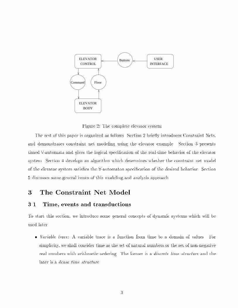
consists of ELEVATOR BODY, ELEVATOR CONTROL and USER INTERFACE as shown

in Fig. 2.

2

Command Floor

Buttons

ELEVATOR

BODY

ELEVATOR

CONTROL

USER

INTERFACE

Figure 2: The complete elevator system

The rest of this paper is organized as follows. Section 2 brie y introduces Constraint Nets,

and demonstrates constraint net modeling using the elevator example. Section 3 presents

timed 8-automata and gives the logical speci�cation of the real-time behavior of the elevator

system. Section 4 develops an algorithm which determines whether the constraint net model

of the elevator system satis�es the 8-automaton speci�cation of the desired behavior. Section

5 discusses some general issues of this modeling and analysis approach.

3 The Constraint Net Model

3.1 Time, events and transductions

To start this section, we introduce some general concepts of dynamic systems which will be

used later.

� Variable trace: A variable trace is a function from time to a domain of values. For

simplicity, we shall consider time as the set of natural numbers or the set of non-negative

real numbers with arithmetic ordering. The former is a discrete time structure and the

later is a dense time structure.

3

� Event trace: An event trace is a variable trace whose domain is boolean. An event in any

event trace is a transition from 0 to 1 or 1 to 0.

� Transduction: A transduction is a mapping from a tuple of input traces to an output

trace which is causal, viz. the output value at any time is determined by the input values

prior to or at that time. Transductions can be considered as transformational processes.

For example, a temporal integration is a transduction. We will see that any deterministic

automaton de�nes a transduction. Clearly, transductions are closed under composition.

Transductions are the basic concept in on-line models, analogous to functions in o�-line

models. Transliterations and delays are two elementary types of transductions for dynamic

systems.

� Transliteration: A transliteration fT is a pointwise extension of function f , that is, the

output value at any time is the function applied to the input value at that time. Let v

be the input variable trace then we have fT (v) = �t:f(v(t)).

� Unit delay: A unit delay �(init) is a transduction de�ned on discrete time structures. Let

v be the input variable trace then we have

�(init)(v) = �k:

(init if k = 0

v(k � 1) otherwise:

� Transport delay: A transport delay �(�)(init), where � � 0 is a real number, is a trans-

duction de�ned on dense time structures. Let v be the input variable trace then we

have

�(�)(init)(v) = �t:

(init if t < �

v(t� �) otherwise:

� Event-driven transductions: any transduction de�ned on a discrete time structure can

be extended to an event-driven transduction with an additional input of an event trace.

The set of events in the event trace becomes the time structure of the transduction. The

output value of the transduction holds between events.

4

� Dynamics of robotic system: A robotic system consists of a robot coupled to its environ-

ment. A robot is composed of a plant coupled to a controller. In Fig. 2, ELEVATOR

BODY is the plant, ELEVATOR CONTROL is the controller and USER INTERFACE

is the environment. A robotic system can be modeled as a set of transductions. For the

elevator example we have

FloorTrace = Elevator (CommandTrace)

CommandTrace = Control (ButtonsTrace; F loorTrace)

ButtonsTrace = Interface ()

The overall behavior of the system is not determined by any one of the transduction alone,

but emerges from the coupling of the interactions among all the transductions. Formally,

the trajectory of the system is the solution of the set of equations.

3.2 Constraint nets

A constraint net is a triple CN � hLc; Td;Cni, where Lc is a set of locations, Td is a set of

transductions, each of which is associated with a tuple of input ports and an output port ; Cn

is a set of directed connections between locations and ports of transductions. Topologically, a

constraint net is a bipartite directed graph where locations are represented by circles, trans-

ductions are represented by boxes and connections are represented by arcs, each from a port

of a transduction to a location or vice versa. A location is an input i� there is no connection

pointing to it otherwise it is an output . For a constraint net CN , the set of input locations is

denoted by I(CN), the set of output locations is denoted by O(CN). A constraint net is closed

i� there are no input locations otherwise it is open.

Semantically, a constraint net is a set of equations on a set of variables corresponding to

Lc, where each left-hand side is an individual output location and each right-hand side is an

expression composed of transductions and locations. The semantics of a constraint net is de�ned

to be the least �xpoint of the set of equations [12].

5

Amodule is a tripleCN(I;O) where CN is a constraint net, I � I(CN) (resp. O � O(CN))

is a subset of the input (resp. output) locations of CN ; I[O de�nes the interface of the module.

Complex modules can be hierarchically constructed from simple ones using three operations:

composition, coalescence and hiding [12].

4 A Discrete Model of the Elevator System

We can model dynamic systems at any level of abstraction in constraint nets. For the elevator

example, we shall �rst design a control strategy where discrete modeling is appropriate. In this

example, each atomic action of the elevator takes one time unit.

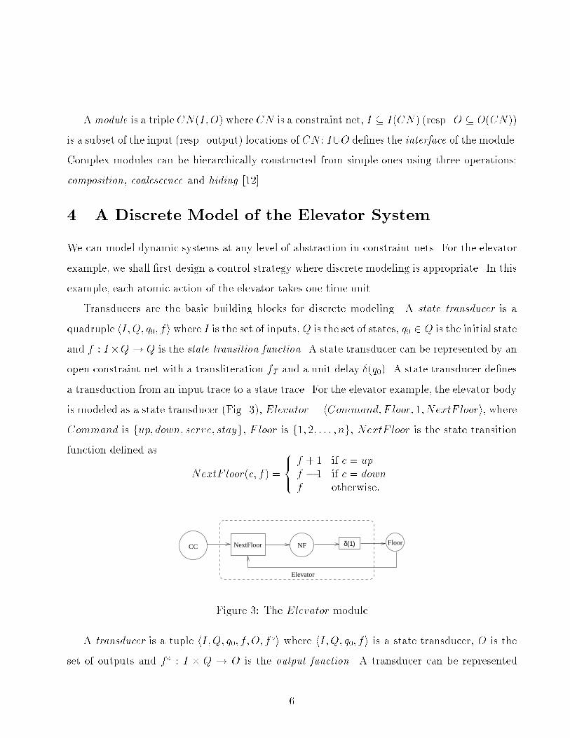
Transducers are the basic building blocks for discrete modeling. A state transducer is a

quadruple hI;Q; q0; fi where I is the set of inputs, Q is the set of states, q0 2 Q is the initial state

and f : I�Q! Q is the state transition function. A state transducer can be represented by an

open constraint net with a transliteration fT and a unit delay �(q0). A state transducer de�nes

a transduction from an input trace to a state trace. For the elevator example, the elevator body

is modeled as a state transducer (Fig. 3), Elevator = hCommand; F loor; 1; NextF loori; where

Command is fup; down; serve; stayg, Floor is f1; 2; : : : ; ng, NextF loor is the state transition

function de�ned as

NextF loor(c; f) =

8><>:f + 1 if c = up

f � 1 if c = down

f otherwise:

Floorδ(1)NF

Elevator

NextFloorCC

Figure 3: The Elevator module

A transducer is a tuple hI;Q; q0; f;O; foi where hI;Q; q0; fi is a state transducer, O is the

set of outputs and fo : I � Q ! O is the output function. A transducer can be represented

6

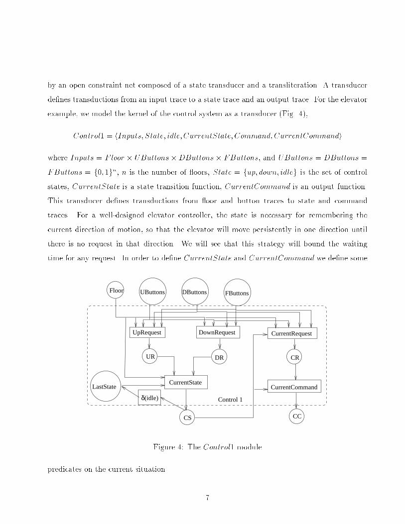
by an open constraint net composed of a state transducer and a transliteration. A transducer

de�nes transductions from an input trace to a state trace and an output trace. For the elevator

example, we model the kernel of the control system as a transducer (Fig. 4),

Control1 = hInputs; State; idle;CurrentState; Command;CurrentCommandi

where Inputs = Floor � UButtons�DButtons � FButtons, and UButtons = DButtons =

FButtons = f0; 1gn, n is the number of oors, State = fup; down; idleg is the set of control

states, CurrentState is a state transition function, CurrentCommand is an output function.

This transducer de�nes transductions from oor and button traces to state and command

traces. For a well-designed elevator controller, the state is necessary for remembering the

current direction of motion, so that the elevator will move persistently in one direction until

there is no request in that direction. We will see that this strategy will bound the waiting

time for any request. In order to de�ne CurrentState and CurrentCommand we de�ne some

Floor UButtons DButtons FButtons

UR CRDR

CS CC

δ(idle) Control 1

LastState CurrentCommand

CurrentRequestDownRequestUpRequest

CurrentState

Figure 4: The Control1 module

predicates on the current situation.

7

� UR indicates whether or not there is any request for the elevator to go up:

UR = UpRequest(f; ub; db; fb)

= ub(f)_i>f

(ub(i) _ db(i) _ fb(i)):

� DR indicates whether or not there is any request for the elevator to go down:

DR = DownRequest(f; ub; db; fb)

= db(f)_i<f

(ub(i) _ db(i) _ fb(i)):

The state transition function can be de�ned as follows:

CS = CurrentState(f; ub; db; fb; ls)

=

8><>:up if UR ^ (ls 6= down _ :DR)

down if (:UR ^ f > 1) _ (DR ^ ls = down)

idle otherwise:

In English, if there is a request for the elevator to go up and either the last state is up or there

is no request to go down, the elevator will be in the up state; if there is no request to go up

and the elevator is not at the �rst oor, or the last state is down and there is a request to go

down, then the elevator will be in the down state; otherwise the elevator will be idle, that is,

the elevator will be parked at the �rst oor if there are no more requests.

Let CR indicates whether or not there is any request for the elevator to stop and serve the

current oor:

CR = CurrentRequest(f; ub; db; fb; ls)

=

(db(f) _ fb(f) if CS = down

ub(f) _ fb(f) otherwise:

In English, if there is an internal request to arrive at this oor or there is an external request

to go in the same direction as the elevator, there is a request at this oor.

The output function can be de�ned as follows:

CC = CurrentCommand(f; ub; db; fb; ls)

=

(serve if CR

CS otherwise:

8

In English, if there is a request at this oor, the elevator will stop to serve the oor (open the

door, let passagers to go in and out, then close the door), otherwise the elevator will pass this

oor without stopping.

Generalizing, we can model a discrete dynamic system in a constraint net composed only of

transliterations and unit delays. Any output location of a unit delay is called a state location.

To model the complete control of the elevator system, we need to de�ne another two modules

which turn o� the corresponding button when the request is served. We use a tuple of ip- ops

for this purpose. A ip- op is a transducer with the �rst input as set and the second input as

reset. Formally,

FlipF lop(set; reset; state) =

8><>:

0 if reset

1 otherwise if set

state otherwise:

A unit delay is added to form the transducer (Fig. 5(a)). This ip op is designed so that

reset has higher priority than set. For the elevator example, this means that the elevator can

not stop for more than one unit time.

The reset signals are created by the ClearBoard module (Fig. 5(b)) which sets the corre-

sponding bit when the request is served.

Summarizing, the elevator system is a constraint net composed of four modules: Elevator,

Control1, FlipF lop and ClearBoard (Fig. 6). We have implemented the discrete model of the

elevator system in Strand88 [4], a concurrent logic programming language (Appendix A.1). It

is easy to simulate discrete constraint nets in Strand88 where a variable trace is an in�nite list,

and both transliterations and unit delays can be represented.

%f(+in, -out) is a function. fT(+in_trace, -out_trace) is a transliteration.

fT([I|Is], OS) :- f(I, O), OS := [O|Os], fT(Is, Os).

%delay(+init, +in_trace, -out_trace)

delay(Init, In, Out) :- Out := [Init|In].

9

Floor CS CC

Clear

δ(0)

CButtons

IButtons

δ(0)SButtons

Buttons CButtons

(b)(a)

ClearBoard

FlipFlop

FlipFlop

Figure 5: (a) The FlipF lop module (b) The ClearBoard module

CButtons

CC

IButtons CS

Floor

Buttons

Control

ClearBoard

FlipFlop

Elevator

Control 1

Figure 6: The constraint net of the elevator system

10

5 A More Realistic Model in Constraint Nets

More details should be considered for designing a real elevator system. In the previous modeling

of the elevator system, atomic actions are primitives. Now we shall model how these actions

are carried out by the lower level control system, which is modeled as an analog controller.

Many physical systems and analog control systems are better modeled as di�erential equations

in dense time structures. Now we shall model how the discrete event-driven controller interacts

with the continuous dynamic system.

A dynamic system in a dense time structure can be modeled by constraint nets composed

of transliterations, transport delays and event-driven transductions. In continuous modeling,

we always consider integration as a basic transduction, even though it can be de�ned in terms

of a limiting behavior generated by an in�nitesimal transport delay.

We have implemented this more realistic model of the elevator system in ALERT, A Labora-

tory of Embedded Real-Time systems, developed in Simulink. ALERT is a visual programming

and simulation environment based on the semantics of constraint nets. ALERT consists of var-

ious building blocks, from simple modules of event logics, linear and nonlinear transductions to

complex constraint solvers. ALERT provides hierarchical structures for constructing complex

modules from simple ones.

The overall structure of the elevator system modeled in ALERT is shown in Fig. 7.

For this more realistic modeling, the Elevator module is further decomposed into two mod-

ules. One is the body of the elevator described by Newton's Law F �KV_h = �h where F is the

motor force, KV is the friction coe�cient and h is the current height of the elevator (Fig. 8).

(We assume the mass is 1 since it can be scaled by F and KV . We ignore the constant force of

gravity since it can be added to F to compensate.) This module de�nes a transduction from

the force trace to the height trace.

The other module is the lower level controller of the elevator. Control0 transforms com-

mands from the higher level controller Control1 into forces to drive the elevator and sends back

the state of the elevator, which are the current oor number and whether or not the elevator

11

Figure 7: The elevator system in ALERT (Locations are not explicitly represented here; how-

ever, any wire is interpreted as a location. Scopes are display devices.)

12

Figure 8: The dynamics of the elevator body

is close to the oor (within 15 cm), to the higher level controller and the event generator. Fig.

9 shows the lower level controller where commands up, down and stop are 1, �1 and 0 respec-

tively. For up and down, a constant force is applied; for stop, proportional control is applied

where KP is the gain. (KP should be chosen so that the elevator can stop at the oor within a

speci�ed error.) An arbitration is used to combine the two according to the current command.

This controller can be implemented in analog circuits.

Control1, ClearBoard and FlipF lops function in the same way as in the discrete model.

However, ClearBoard and FlipF lops are digital circuits implemented at a fast sampling rate

(0.1 sec.) so that any input signal can be responded to quickly. Control1 is now an event-driven

transduction where events are generated by the event module in Fig. 10.

There are three basic types of events: (1) someone pushes a button in the elevator's idle

state, (2) the elevator becomes close to a oor (within 15 cm) and (3) the elevator has served

the oor for a certain time; the time of the transport delay (say 4 sec.) is the time for serving

the oor. The \event or" of these three events excites the Control1 module to produce a new

output.

13

Figure 9: The lower level analog control

6 The Timed 8-Automaton Speci�cation

While modeling focuses on the underlying structure of a system, the organization and coordina-

tion of components or subsystems, the overall behavior of the modeled system is not explicitly

expressed. However, for many situations, it is important to specify some global properties

and guarantee that these properties hold in this design. For example, a well-designed elevator

system should service any request within a bounded waiting time.

A logical speci�cation can serve this purpose. In this section, we shall present timed 8-

automata for specifying behaviors in discrete time structures, and demonstrate how to use this

logical speci�cation to state desired properties of an elevator system.

6.1 State formulas

A state formula Fs is a �rst-order formula:

Fs � false j T1 = T2 j p(T1; : : : ; Tn) j Fs1 ! Fs2 j9xFs

14

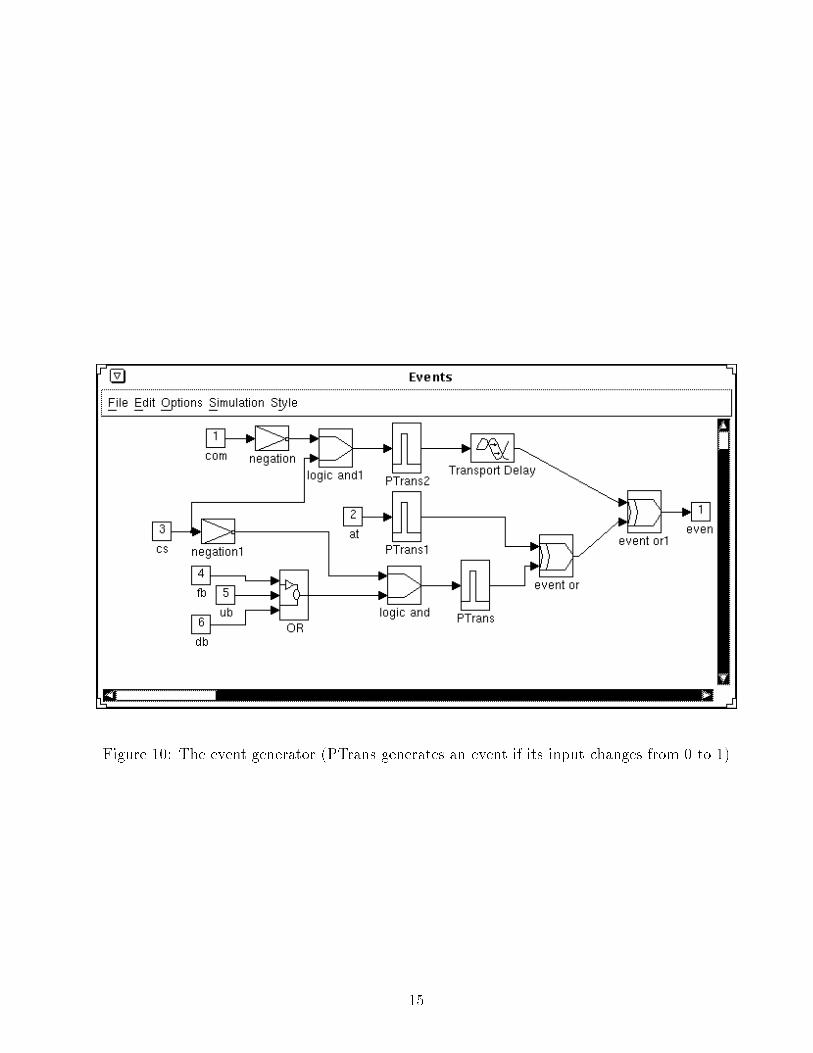
Figure 10: The event generator (PTrans generates an event if its input changes from 0 to 1)

15

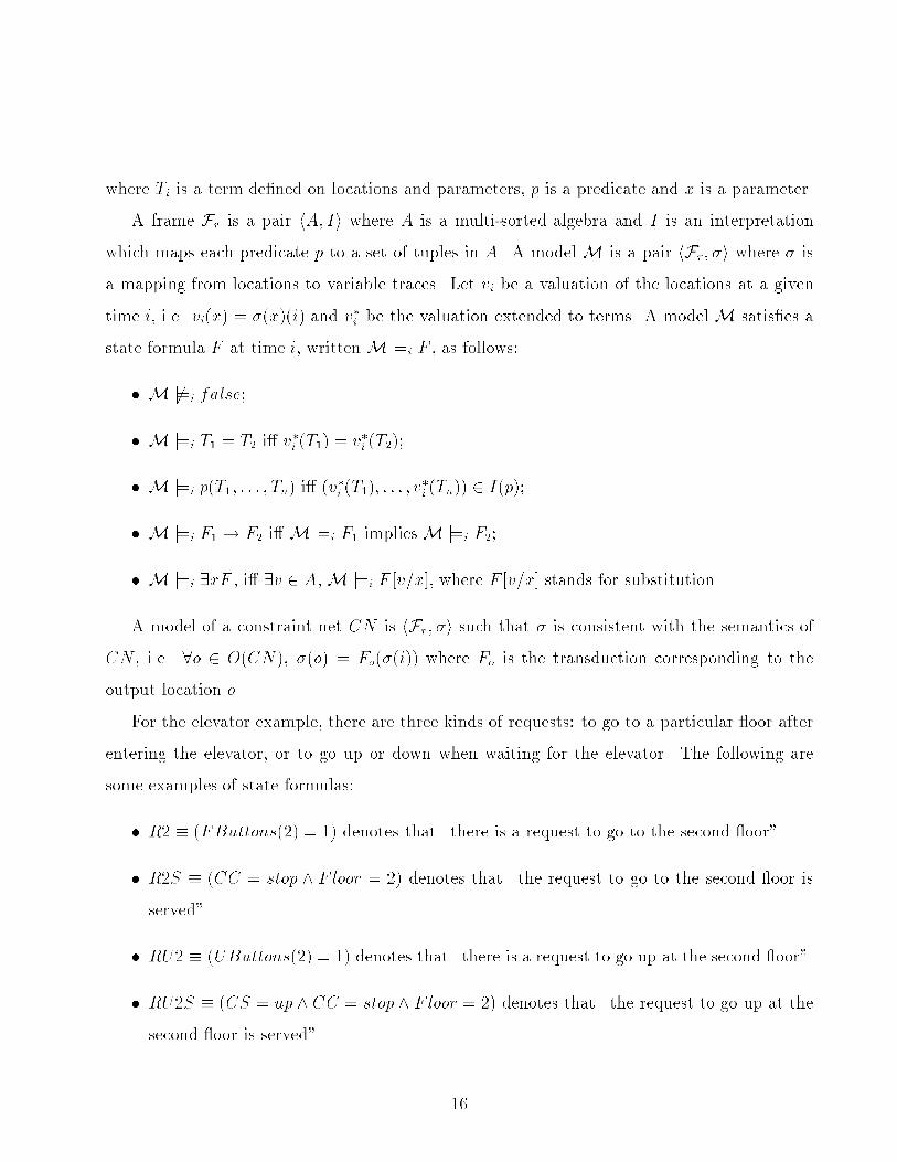
where Ti is a term de�ned on locations and parameters, p is a predicate and x is a parameter.

A frame Fr is a pair hA; Ii where A is a multi-sorted algebra and I is an interpretation

which maps each predicate p to a set of tuples in A. A model M is a pair hFr; �i where � is

a mapping from locations to variable traces. Let vi be a valuation of the locations at a given

time i, i.e. vi(x) = �(x)(i) and v�ibe the valuation extended to terms. A model M satis�es a

state formula F at time i, written M j=i F , as follows:

� M 6j=i false;

� M j=i T1 = T2 i� v�i(T1) = v

�i(T2);

� M j=i p(T1; : : : ; Tn) i� (v�i(T1); : : : ; v

�i(Tn)) 2 I(p);

� M j=i F1 ! F2 i� M j=i F1 impliesM j=i F2;

� M j=i 9xF , i� 9v 2 A,M j=i F [v=x], where F [v=x] stands for substitution.

A model of a constraint net CN is hFr; �i such that � is consistent with the semantics of

CN , i.e. 8o 2 O(CN), �(o) = Fo(�(i)) where Fo is the transduction corresponding to the

output location o.

For the elevator example, there are three kinds of requests: to go to a particular oor after

entering the elevator, or to go up or down when waiting for the elevator. The following are

some examples of state formulas:

� R2 � (FButtons(2) = 1) denotes that \there is a request to go to the second oor".

� R2S � (CC = stop ^ Floor = 2) denotes that \the request to go to the second oor is

served".

� RU2 � (UButtons(2) = 1) denotes that \there is a request to go up at the second oor".

� RU2S � (CS = up ^ CC = stop ^ Floor = 2) denotes that \the request to go up at the

second oor is served".

16

6.2 Timed 8-automaton

A 8-automaton [8] A is a quintuple hQ;R; S; e; ci where Q is a �nite set of automaton states,

R � Q is a set of recurrent states and S � Q is a set of stable states. Let Fs be the set of

state formulas, e : Q ! Fs is an entry condition function such thatWq2Q e(q) = true, and

c : Q�Q! Fs is a transition condition function such that 8q 2 Q;Wq02Q c(q; q

0) = true. A run

of A over a modelM on a discrete time structure is a sequence of states q0; q1; q2; : : : such that

(1) M j=0 e(q0); and (2) for all time points i > 0, M j=i c(qi�1; qi). Let Inf(r) � Q denote

the set of automaton states that appear in�nitely many times in r. A run r is de�ned to be

accepting i�: (a) Inf(r) \ R 6= ;; or (b) Inf(r) � S. A 8-automaton A accepts a model M,

writtenM j= A, i� all possible runs ofA overM are accepting. A accepts a constraint net CN ,

written CN j= A, i� A accepts all models of CN . It has been shown [8] that the speci�cation

power of 8-automata is identical to that of ETL, an extended linear discrete temporal logic

[11].

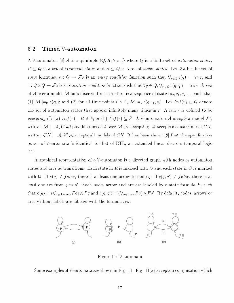
A graphical representation of a 8-automaton is a directed graph with nodes as automaton

states and arcs as transitions. Each state in R is marked with 3 and each state in S is marked

with 2. If e(q) 6= false, there is at least one arrow to node q. If c(q; q0) 6= false, there is at

least one arc from q to q0. Each node, arrow and arc are labeled by a state formula F , such

that e(q) = (Wa2Arrows Fa)^Fq and c(q; q

0) = (Wa2Arcs Fa)^Fq

0. By default, nodes, arrows or

arcs without labels are labeled with the formula true.

P

R

E

E

P

(a) (b) (c)

E

R

E

P P

P

Figure 11: 8-automata

Some examples of 8-automata are shown in Fig. 11. Fig. 11(a) accepts a computation which

17

satis�es :P only �nitely many times, Fig. 11(b) accepts a computation which never satis�es

P and Fig. 11(c) accepts a computation which will satisfy R in the �nite future whenever it

satis�es E.

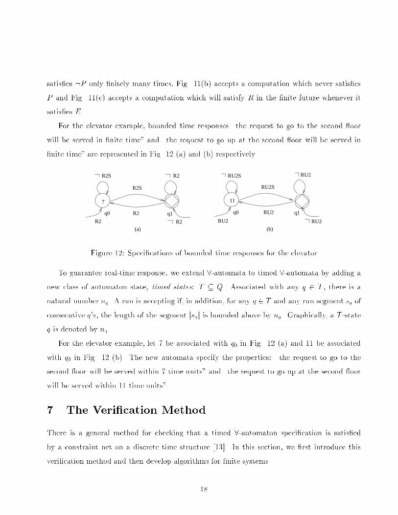
For the elevator example, bounded time responses \the request to go to the second oor

will be served in �nite time" and \the request to go up at the second oor will be served in

�nite time" are represented in Fig. 12 (a) and (b) respectively.

R2S R2

R2 RU2

RU2

RU2S

RU2

RU2S

(a) (b)

q1q0 q0 q1

R2

R2S

R2 RU2

7 11

Figure 12: Speci�cations of bounded time responses for the elevator

To guarantee real-time response, we extend 8-automata to timed 8-automata by adding a

new class of automaton state, timed states: T � Q. Associated with any q 2 T , there is a

natural number nq. A run is accepting if, in addition, for any q 2 T and any run segment sq of

consecutive q's, the length of the segment jsqj is bounded above by nq. Graphically, a T -state

q is denoted by nq.

For the elevator example, let 7 be associated with q0 in Fig. 12 (a) and 11 be associated

with q0 in Fig. 12 (b). The new automata specify the properties: \the request to go to the

second oor will be served within 7 time units" and \the request to go up at the second oor

will be served within 11 time units".

7 The Veri�cation Method

There is a general method for checking that a timed 8-automaton speci�cation is satis�ed

by a constraint net on a discrete time structure [13]. In this section, we �rst introduce this

veri�cation method and then develop algorithms for �nite systems.

18

7.1 The general method

Let S be the set of state locations, O = O(CN)nS be the set of the other output locations,

I = I(CN) be the set of input locations and A be the domain of values. Generally, a constraint

net on a discrete time structure can be written as two sets of equations: s0 = fs(i; s); o = fo(i; s)

where s,s0 : S ! A is a state tuple, i : I ! A is an input tuple, fs is a tuple of state transition

functions, o : O ! A is an output tuple, and fo is a tuple of output functions. Therefore, such

a constraint net is globally a transducer hI;S; s0; fs;O; foi where I = fiji : I ! Ag is the set

of inputs, S = fsjs : S ! Ag is the set of states, s0 is the initial state, fs is the state transition

function, O = fojo : O ! Ag is the set of outputs and fo is the output function.

We write f'gCNf g to denote the veri�cation condition:

'[fo(i; s)=o]^s0 = fs(i; s)! [i0=i; s0=s; fo(i

0; s

0)=o]

where ' and are state formulas; ' characterizes pre-conditions and indicates post-conditions.

For example, if ES is the elevator system in Fig. 6, we have

fFButton(2) = 1 ^ CC = down ^ Floor = 3gESfFButton(2) = 0g

Model checking of a constraint net CN against its speci�cation A involves three phases:

Phase 1: Associate with each automaton state q 2 Q an assertion �q 2 Ls, called the invariant

at q, such that the following requirements are satis�ed:

� Initiality: [s0 ^ e(q)]! �q;8q 2 Q.

� Consecution: f�qgCNfc(q; q0)! �q0g, 8q; q0 2 Q.

Phase 2: Associate with each automaton state q 2 Q a ranking function �q : I �S !W, where

W is a well-founded set, i.e., 8w0 2 W, any decreasing sequence w0 > w1 > : : : is �nite, such

that the following requirements are satis�ed:

� De�nedness: �q ! 9w:�q = w;8q 2 Q.

19

� Non-increase: f�q ^ �q = wgCNfc(q; q0)! �q0 � wg;8q0 2 S.

� Decrease: f�q ^ �q = wgCNfc(q; q0)! �q0 < wg;8q0 2 Qn(R [ S).

Phase 3: Associate with each q 2 T a timing function, q : I � S ! N where N is the set of

natural numbers, such that the following requirements are satis�ed:

� Boundedness: �q ! 1 � q � nq, 8q 2 T ;

� Decrease: f�q ^ q = wgCNfc(q; q)! q < wg;8q 2 T .

The veri�cation rule is sound and complete, that is, if we succeed in �nding invariants �q, a

well-founded setW, ranking functions �q and timing functions q, such that all the requirements

are satis�ed, then this establishes the validity of A over CN ; on the other hand, if A is valid

over CN , then there are invariants �q, a well-founded set W, ranking functions �q and timing

functions q, such that all the requirements are satis�ed [8].

7.2 The algorithm

A constraint net is �nite i� the domain of values is �nite. For example, �nite state transducers

are represented by �nite constraint nets. Digital sequential circuits can be represented by

�nite constraint nets since the domain of values, boolean, is �nite. We can automate the model

checking process for �nite constraint nets as long as f�qg is known as a priori. A �nite constraint

net is a transducer of �nite input-state pairs. For each q 2 Q, e(q) and �q corresponds to a set

of input-state pairs of the constraint net. For each q; q0 2 Q, c(q; q0) corresponds to a binary

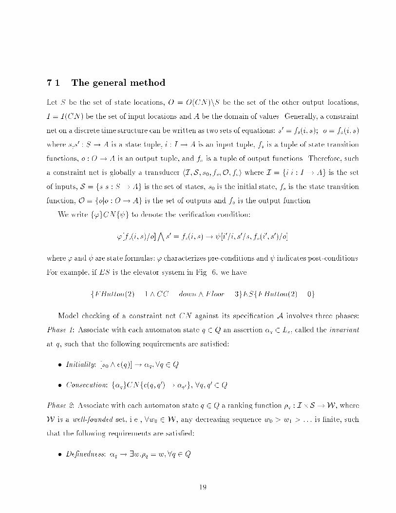
relation of the input-state pairs. The algorithm consists of three phases: (1) Initiality and

Consecution, (2) Ranking and (3) Timing.

The algorithm for the �rst phase is a direct translation of the veri�cation rules (Fig. 13).

The algorithm of the second phase consists of two steps. The �rst step of this algorithm

is to generate a state transition graph. An input-state pair (i; s) is in the graph i� �q(i; s)

for some stable or bad automaton state q. There is a transition between (i; s) and (i0; s0) i�

20

||||||||||||||||||||||||||

Algorithm: Initiality and Consecution

for all q in Q do

if not itest(q) return false

for all q, q' in Q do

if not ctest(q, q') return false

itest(q):

for all input i and initial state s0 do

if e(q)(i,s0) and not a(q)(i,s0)

return false

return true

ctest(q, q'):

for all (i,s) and (i',s') do

if a(q)(i,s) and s'=fs(i,s) and c(q,q')(i,s,i',s') and

not a(q')(i',s') return false

return true

||||||||||||||||||||||||||-

Figure 13: The algorithm for initiality and consecution

21

�q(i; s) ^ �q0(i0; s0) ^ c(q; q0)(i; s; i0; s0). An input-state pair (i; s) is called bad i� �q(i; s) for

some bad automaton-state q. The property of the graph we want to check is: there is no loop

consisting of any bad input-state pairs (Fig. 14).

||||||||||||||||||||||||||-

Algorithm: Ranking

1. /* Generate a state transition graph <V,E> */

for all q in B = Q \ R do

for all (i,s) do

if a(q)(i,s) put (i,s) in V

for all q, q' in Q \ R do

for all (i,s) and (i',s') do

if a(q)(i,s) and s' = fs(i,s) and c(q,q')(i,s,i',s')

put (i,s,i',s') in E

2. /* Check the acyclicity of bad states in <V,E> */

for all (i,s) in V with a(q)(i,s) for some bad state q do

for all path p from (i,s) do

if p ends at (i,s) return false

return true

||||||||||||||||||||||||||-

Figure 14: The algorithm for ranking

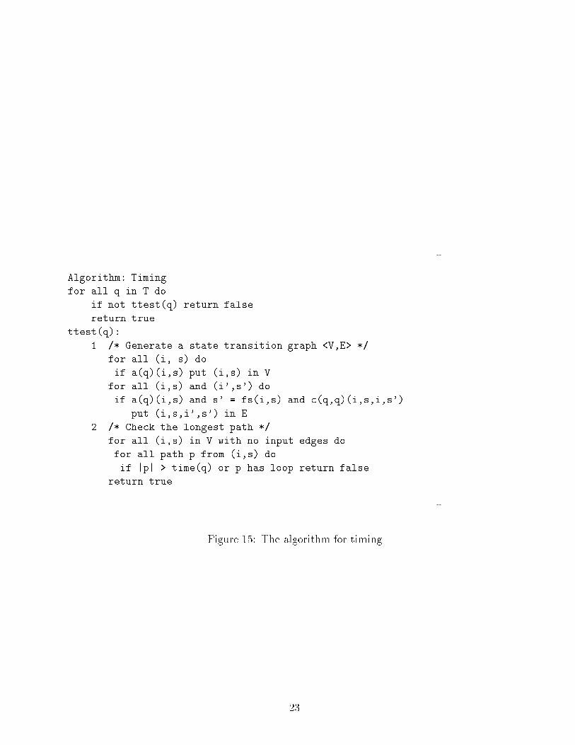
The algorithm of the third phase is similar to the second phase except that we need to check

the maximum length of each timed state in all the transition paths in the graph (Fig. 15).

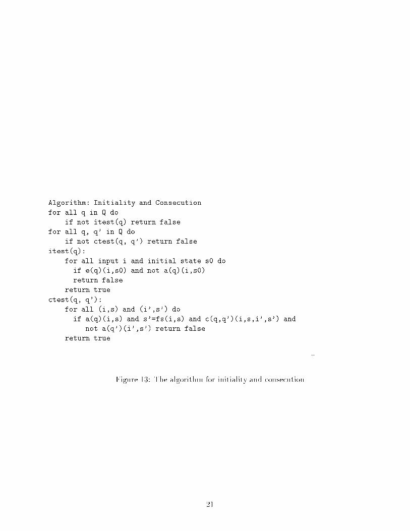
We have implemented this model checking algorithm in Quintus Prolog (Appendix A.2).

The speci�cations in the previous section are checked out using this algorithm by letting �q0 =

R2 (resp. RU2) and �q1 = R2S (resp. RU2S). The discrete constraint net model of the

elevator system is given in \liftimp.pl" (Appendix A.3); the timed 8-automata are speci�ed

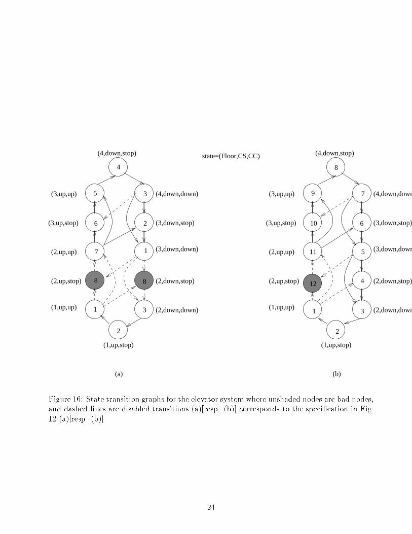
in \liftspe1.pl" and \liftspe2.pl" respectively (Appendix A.4). If n = 4, the state transition

graphs for the elevator controller are shown in Fig. 16 (a) and (b) respectively, where dashed

transitions are disabled in our control strategy. For simplicity, a state in the graph is a cluster

of input-state pairs.

22

||||||||||||||||||||||||||-

Algorithm: Timing

for all q in T do

if not ttest(q) return false

return true

ttest(q):

1. /* Generate a state transition graph <V,E> */

for all (i, s) do

if a(q)(i,s) put (i,s) in V

for all (i,s) and (i',s') do

if a(q)(i,s) and s' = fs(i,s) and c(q,q)(i,s,i,s')

put (i,s,i',s') in E

2. /* Check the longest path */

for all (i,s) in V with no input edges do

for all path p from (i,s) do

if |p| > time(q) or p has loop return false

return true

||||||||||||||||||||||||||-

Figure 15: The algorithm for timing

23

(1,up,up)

(2,up,stop)

(2,up,up)

(3,up,stop)

(3,up,up)

(1,up,stop)

(4,down,down)

(3,down,stop)

(3,down,down)

(2,down,stop)

(2,down,down) (1,up,up)

(2,up,stop)

(2,up,up)

(3,up,stop)

(3,up,up)

(1,up,stop)

(4,down,down

(3,down,stop)

(3,down,down

(2,down,stop)

(2,down,down

state=(Floor,CS,CC)

(a) (b)

7

2

1 3

8

1

2

3

4

5

6

8

2

1 3

4

5

6

7

8

9

10

11

12

(4,down,stop) (4,down,stop)

Figure 16: State transition graphs for the elevator system where unshaded nodes are bad nodes,

and dashed lines are disabled transitions (a)[resp. (b)] corresponds to the speci�cation in Fig.

12 (a)[resp. (b)].

24

8 Conclusions

We have discussed modeling and analysis in the context of an elevator system. Now we shall

make some general comments on this approach and draw some conclusions.

8.1 Modeling

An appropriate model of behavioral dynamics in robotic systems should satisfy the following

properties (modi�ed from [7, 10]):

� it is a real-time model where time can be represented explicitly;

A robot coupled to its environment is a complex dynamic system. The interaction between

the robot and the environment is often constrained by time.

� it can model the dynamics of the environment as well as the the dynamics of the plant

and the dynamics of the control;

A robot is an open system. The behavior of the system is meaningless without considering

the dynamics of its environment. It is important to represent the structural congruence

between the dynamics of the system and the dynamics of its external environment, i.e.

to model the environment as a machine.

� it can represent dense, as well as discrete, dynamic systems, asynchronous processes, and

the coordination of processes with di�erent dynamics;

The control system of a robot may consist of multiple components with both analog and

digital circuits. The communication between di�erent counterparts may incorporate both

time-driven and event-driven conventions.

� it can provide multiple levels of abstraction.

Like most complex systems, the organization of control systems should be modular and

hierarchical. With this organization, a system can be incrementally designed, debugged

and veri�ed.

25

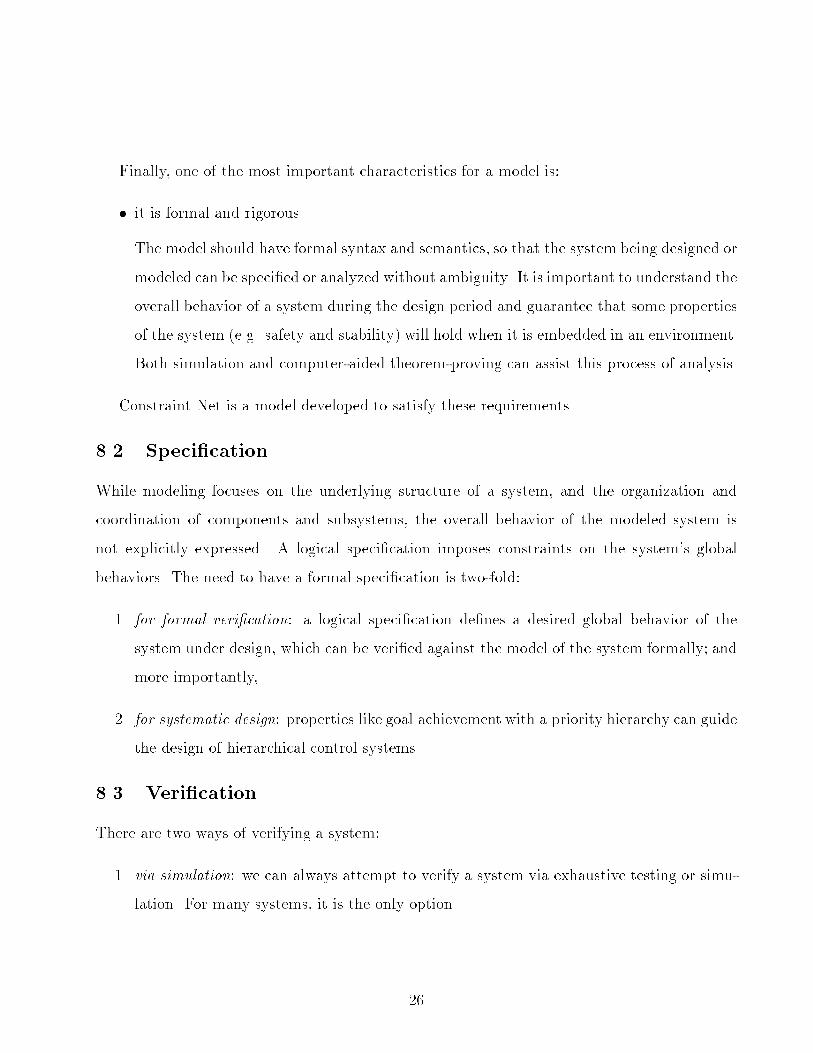
Finally, one of the most important characteristics for a model is:

� it is formal and rigorous.

The model should have formal syntax and semantics, so that the system being designed or

modeled can be speci�ed or analyzed without ambiguity. It is important to understand the

overall behavior of a system during the design period and guarantee that some properties

of the system (e.g. safety and stability) will hold when it is embedded in an environment.

Both simulation and computer-aided theorem-proving can assist this process of analysis.

Constraint Net is a model developed to satisfy these requirements.

8.2 Speci�cation

While modeling focuses on the underlying structure of a system, and the organization and

coordination of components and subsystems, the overall behavior of the modeled system is

not explicitly expressed. A logical speci�cation imposes constraints on the system's global

behaviors. The need to have a formal speci�cation is two-fold:

1. for formal veri�cation: a logical speci�cation de�nes a desired global behavior of the

system under design, which can be veri�ed against the model of the system formally; and

more importantly,

2. for systematic design: properties like goal achievement with a priority hierarchy can guide

the design of hierarchical control systems.

8.3 Veri�cation

There are two ways of verifying a system:

1. via simulation: we can always attempt to verify a system via exhaustive testing or simu-

lation. For many systems, it is the only option.

26

2. via formal veri�cation: for discrete time systems, computer-aided model checking or the-

orem proving is possible. Furthermore, for �nite systems automatic veri�cation can be

achieved.

However, neither simulation nor formal veri�cation is su�cient to guarantee well-behavedness.

First, the model is only an abstraction of the real system, the real system probably has unmod-

eled aspects which may cause problems. Second, the speci�cation maybe incomplete: it is hard

to enumerate all the desired properties, and there maybe properties which are not expressible

in the given speci�cation language.

Even though veri�cation is not su�cient, it will decrease run-time problems for the designed

system. Proper system design is based on an appropriate level of abstraction and a su�cient

set of desired properties.

Acknowledgements: Thanks to Peter Caines, Hector Levesque, Ray Reiter and Maarten

van Emden for stimulating us to work on this problem. This work was supported in part by the

Natural Sciences and Engineering Research Council, the Institute for Robotics and Intelligent

Systems and the Canadian Institute for Advanced Research.

References

[1] H. Barringer. Up and down the temporal way. Technical report, University of Manchester,

England, September 1985.

[2] P.E. Caines, T. Mackling, and Y.J. Wei. A logical controller for CIAR1 elevator system

by cocolog, 1992. Unpublished.

[3] D.N. Dyck and P.E. Caines. The logical control of an elevator, 1992. Unpublished.

[4] I. Foster and S. Taylor. Strand: New Concepts in Parallel Programming. Prentice Hall,

1989.

[5] R. Hale. Using temporal logic for prototyping: The design of a lift controller. In H.S.M.

Zedan, editor, Real-Time Systems, Theory and Applications. Elsvier Science Publishers

B.V. (North-Holland), 1990.

27

[6] M.A. Jackson. System Development. Prentice-Hall, Englewood Cli�s, 1983.

[7] J. Lavignon and Y. Shoham. Temporal automata. Technical Report STAN-CS-90-1325,

Robotics Laboratory, Computer Science Department, Stanford University, Stanford, CA

94305, 1990.

[8] Z. Manna and A. Pnueli. Speci�cation and veri�cation of concurrent programs by 8-

automata. In Proc. 14th Ann. ACM Symp. on Principles of Programming Languages,

pages 1{12, 1987.

[9] B. Sanden. An entity-life modeling approach to the design of concurrent software. Com-

munication of the ACM, 32(3):230 { 243, March 1989.

[10] Y. Shoham. Agent-oriented programming. Technical Report STAN-CS-1335-90, Computer

Science Department, Stanford University, 1990.

[11] P. Wolper. Temporal logic can be more expressive. Information and Control, 56:72 { 99,

1983.

[12] Y. Zhang and A. K. Mackworth. Constraint Nets: A semantic model of real-time embedded

systems. Technical Report 92-10, Department of Computer Science, University of British

Columbia, 1992.

[13] Y. Zhang and A. K. Mackworth. Will the robot do the right thing? Technical Report

92-31, Department of Computer Science, University of British Columbia, 1992.

28

A Appendix

A.1 Strand88 Implementation

-compile(free).

-exports([commTd/6, clearT/6, floorTd/2, board/4, boardTd/3, system/6]).

%%%%%%%%%%%%%%%%%%%%%%%%%%%%%%%%%%%%%%%%%%%%%%%%%%%%%%%%%%%%%

% Functions %

%%%%%%%%%%%%%%%%%%%%%%%%%%%%%%%%%%%%%%%%%%%%%%%%%%%%%%%%%%%%%

comm(F, LCS, UP, DOWN, OUT, COM, CS) :-

urequest(F, UP, DOWN, OUT, UR),

drequest(F, UP, DOWN, OUT, DR),

currents(F, LCS, UR, DR, CS),

crequest(F, CS, UP, DOWN, OUT, CR),

command(CS, CR, COM).

currents(_, idle, 1, _, CS) :- CS := up.

currents(_, up, 1, _, CS) :- CS := up.

currents(_, down, 1, 0, CS) :- CS := up.

currents(F, _, 0, _, CS) :- F > 1|CS := down.

currents(_, down, _, 1, CS) :- CS := down.

currents(1, _, 0, 0, CS) :- CS := idle.

command(_CS, 1, COM) :- COM := serve.

command(CS, 0, COM) :- COM := CS.

floor(F, down, NF) :- NF is F - 1.

floor(F, up, NF) :- NF is F + 1.

floor(F, serve, NF) :- NF := F.

floor(F, idle, NF) :- NF := F.

clear(F, up, serve, CUP, CDOWN, COUT) :-

reset(4, CDOWN),

clear1(F, COUT),

clear1(F, CUP).

clear(F, down, serve, CUP, CDOWN, COUT) :-

reset(4, CUP),

clear1(F, COUT),

clear1(F, CDOWN).

29

clear(_, _, _, CUP, CDOWN, COUT) :- otherwise|

reset(4, CUP),

reset(4, CDOWN),

reset(4, COUT).

reset(0, X) :- X := [].

reset(I, X) :- I > 0| I1 is I - 1, X := [0|X1], reset(I1, X1).

clear1(F, X) :-

reset(4, X0),

set(F, X0, X).

set(1, [_|X0], X) :- X := [1|X0].

set(N, [0|X0], X) :- N > 1| N1 is N - 1, X := [0|X1], set(N1, X0, X1).

crequest(F, down, _, DOWN, OUT, CR) :-

element(F, DOWN, E1),

element(F, OUT, E2),

or(E1, E2, CR).

crequest(F, _, UP, _, OUT, CR) :- otherwise |

element(F, UP, E1),

element(F, OUT, E2),

or(E1, E2, CR).

urequest(4, _, _, _, UR) :- UR := 0.

urequest(F, UP, DOWN, OUT, UR) :- otherwise |

F1 is F + 1,

element(F, UP, E0),

elements(F1, UP, Es1),

elements(F1, DOWN, Es2),

elements(F1, OUT, Es3),

or(Es1, E1),

or(Es2, E2),

or(Es3, E3),

or([E0, E1, E2, E3], UR).

drequest(1, _, _, _, DR) :- DR := 0.

drequest(F, UP, DOWN, OUT, DR) :- otherwise |

F1 is F - 1,

30

element(F, DOWN, E0),

elemente(F1, UP, Es1),

elemente(F1, DOWN, Es2),

elemente(F1, OUT, Es3),

or(Es1, E1),

or(Es2, E2),

or(Es3, E3),

or([E0, E1, E2, E3], DR).

element(1, [X|_], E) :- E := X.

element(N, [_|Xs], E) :- N > 1| N1 is N - 1, element(N1, Xs, E).

elements(1, X, Es) :- Es := X.

elements(N, [_|Xs], Es) :- N > 1| N1 is N - 1, elements(N1, Xs, Es).

elemente(1, [X|_], Es) :- Es := [X].

elemente(N, [X|Xs], Es) :- N > 1| Es := [X|Es1], N1 is N - 1,

elemente(N1, Xs, Es1).

or(1, _, X) :- X := 1.

or(0, 1, X) :- X := 1.

or(_, _, X) :- otherwise | X := 0.

or([], X) :- X := 0.

or([E|Es], X) :- or(Es, X1), or(E, X1, X).

board([], [], [], NB) :- NB := [].

board([C|Cs], [U|Us], [B|Bs], NBS) :-

ff(C, U, B, NB),

NBS := [NB|NBs],

board(Cs, Us, Bs, NBs).

ff(1, 0, _, NB) :- NB := 0.

ff(_, 1, _, NB) :- NB := 1.

ff(0, 0, B, NB) :- NB := B.

%%%%%%%%%%%%%%%%%%%%%%%%%%%%%%%%%%%%%%%%%%%%%%%%%%%%%%%%%%%%%%%

% Transliterations %

%%%%%%%%%%%%%%%%%%%%%%%%%%%%%%%%%%%%%%%%%%%%%%%%%%%%%%%%%%%%%%%

commT([], [], [], [], [], COMS, NCSS) :- COMS := [], NCSS := [].

commT([F|Fs], [CS|CSs], [UP|UPs], [DOWN|DOWNs], [OUT|OUTs], COMS, NCSS) :-

31

comm(F, CS, UP, DOWN, OUT, COM, NCS),

COMS := [COM|COMs], NCSS := [NCS|NCSs],

commT(Fs, CSs, UPs, DOWNs, OUTs, COMs, NCSs).

floorT([], [], NFS) :- NFS := [].

floorT([F|Fs], [Com|Coms], NFS) :-

floor(F, Com, NF),

NFS := [NF|NFs],

floorT(Fs, Coms, NFs).

clearT([], [], [], CUPS, CDOWNS, COUTS) :-

CUPS := [], CDOWNS := [], COUTS := [].

clearT([F|Fs], [Cs|Css], [Com|Coms], CUPS, CDOWNS, COUTS) :-

clear(F, Cs, Com, CUP, CDOWN, COUT),

CUPS := [CUP|CUPs],

CDOWNS := [CDOWN|CDOWNs],

COUTS := [COUT|COUTs],

clearT(Fs, Css, Coms, CUPs, CDOWNs, COUTs).

boardT([], [], [], NBS) :- NBS := [].

boardT([C|Cs], [U|Us], [B|Bs], NBS) :-

board(C, U, B, NB),

NBS := [NB|NBs],

boardT(Cs, Us, Bs, NBs).

%%%%%%%%%%%%%%%%%%%%%%%%%%%%%%%%%%%%%%%%%%%%%%%%%%%%%%%%%%%%%%%%%%%

% Unit Delay %

%%%%%%%%%%%%%%%%%%%%%%%%%%%%%%%%%%%%%%%%%%%%%%%%%%%%%%%%%%%%%%%%%%%

delay(I, NS, S) :- S := [I|NS].

%%%%%%%%%%%%%%%%%%%%%%%%%%%%%%%%%%%%%%%%%%%%%%%%%%%%%%%%%%%%%%%%%%%

% Transducers %

%%%%%%%%%%%%%%%%%%%%%%%%%%%%%%%%%%%%%%%%%%%%%%%%%%%%%%%%%%%%%%%%%%%

floorTd(Coms, Fs) :-

delay(1, NFs, Fs),

floorT(Fs, Coms, NFs).

commTd(Fs, UPs, DOWNs, OUTs, COMs, CSs) :-

delay(idle, CSs, PCSs),

commT(Fs, PCSs, UPs, DOWNs, OUTs, COMs, CSs).

32

boardTd(Cs, Us, Bs) :-

reset(4, I),

delay(I, Bs, PBs),

boardT(Cs, Us, PBs, Bs).

clearTd(FS, CS, COMS, CUPS, CDOWNS, COUTS) :-

reset(4, IUPS),

reset(4, IDOWNS),

reset(4, IOUTS),

delay(IUPS, NUPS, CUPS),

delay(IDOWNS, NDOWNS, CDOWNS),

delay(IOUTS, NOUTS, COUTS),

clearT(FS, CS, COMS, NUPS, NDOWNS, NOUTS).

%%%%%%%%%%%%%%%%%%%%%%%%%%%%%%%%%%%%%%%%%%%%%%%%%%%%%%%%%%%%%%%%%%%

% Elevator System %

%%%%%%%%%%%%%%%%%%%%%%%%%%%%%%%%%%%%%%%%%%%%%%%%%%%%%%%%%%%%%%%%%%%

system(UUPS, UDOWNS, UOUTS, FS, COMS, CS) :-

boardTd(CUPS, UUPS, UPS),

boardTd(CDOWNS, UDOWNS, DOWNS),

boardTd(COUTS, UOUTS, OUTS),

clearTd(FS, CS, COMS, CUPS, CDOWNS, COUTS),

floorTd(COMS, FS),

commTd(FS, UPS, DOWNS, OUTS, COMS, CS).

A.2 Model Checker in Quintus Prolog (rtmc.pl)

:- dynamic bstate/2, sstate/2, bstrans/4, tstate/2, ttrans/4.

:- ensure_loaded(library(basics)).

%%%%%%%%%%%%%%%%%%%%%%%%%%%%%%%%%%%%%%%%%%%%%%%%%%%%%%%%%%%%%%%%%%%%

% Model Checker %

%%%%%%%%%%%%%%%%%%%%%%%%%%%%%%%%%%%%%%%%%%%%%%%%%%%%%%%%%%%%%%%%%%%%

model_checker :-

initiality,

consecution,

ranking, !,

33

timing.

%%%%%%%%%%%%%%%%%%%%%%%%%%%%%%%%%%%%%%%%%%%%%%%%%%%%%%%%%%%%%%%%%%%%

% Initiality %

%%%%%%%%%%%%%%%%%%%%%%%%%%%%%%%%%%%%%%%%%%%%%%%%%%%%%%%%%%%%%%%%%%%%

initiality :-

setof(Q, isa(Q), Qs),

initiality(Qs).

isa(Q) :-

a(Q, _).

initiality([Q|Qs]) :-

itest(Q),

initiality(Qs).

initiality([]).

itest(Q) :-

e(Q, Pe), !,

a(Q, Pa),

itest(Pe, Pa).

itest(_).

itest(Pe, Pa) :-

ifail(Pe, Pa), !, fail.

itest(_, _).

ifail(P, P) :- !, fail.

ifail(Pe, Pa) :-

start(S),

callP(Pe, [I, S]),

\+ callP(Pa, [I, S]).

%%%%%%%%%%%%%%%%%%%%%%%%%%%%%%%%%%%%%%%%%%%%%%%%%%%%%%%%%%%%%%%%%%%%%%

% Consecution %

%%%%%%%%%%%%%%%%%%%%%%%%%%%%%%%%%%%%%%%%%%%%%%%%%%%%%%%%%%%%%%%%%%%%%%

34

consecution :-

setof((Q, Q1), isc(Q, Q1), Ts),

consecution(Ts).

isc(Q, Q1) :-

c(Q, Q1, _).

consecution([(Q, Q1)|Ts]) :-

ctest(Q, Q1),

consecution(Ts).

consecution([]).

ctest(Q, Q1) :-

c(Q, Q1, Pc),

a(Q, Pa),

a(Q1, Pa1),

ctest(Pa, Pc, Pa1).

ctest(Pa, Pc, Pa1) :-

cfail(Pa, Pc, Pa1), !, fail.

ctest(_, _, _).

cfail(_, P, P) :- !, fail.

cfail(Pa, Pc, Pa1) :-

callP(Pa, [I, S]),

trans(I, S, S1),

callP(Pc, [I, S, I1, S1]),

\+ callP(Pa1, [I1, S1]).

%%%%%%%%%%%%%%%%%%%%%%%%%%%%%%%%%%%%%%%%%%%%%%%%%%%%%%%%%%%%%%%%%%%%

% Ranking %

%%%%%%%%%%%%%%%%%%%%%%%%%%%%%%%%%%%%%%%%%%%%%%%%%%%%%%%%%%%%%%%%%%%%

ranking :-

rinit,

bad(Bq, T),

states(bstate, Bq),

35

stable(Sq),

states(sstate, Sq),

append(Bq, Sq, Qq),

ptrans(bstrans, Qq, Qq),

rtest(T).

rinit :-

retractall(bstate(_,_)),

retractall(sstate(_,_)),

retractall(bstrans(_,_,_,_)).

states(_, []).

states(P, [Q|Qs]) :-

a(Q, Pa),

setof1([I,S], callP(Pa, [I, S]), ISs),

asserts(P, ISs),

states(P, Qs).

asserts(_, []).

asserts(P, [S|Ss]) :-

P1 =.. [P|S],

assert1(P1),

asserts(P, Ss).

assert1(P) :- P, !.

assert1(P) :- assert(P).

ptrans(_, [], _).

ptrans(P, [Q|Qs], Q1s) :-

ptrans1(P, Q, Q1s),

ptrans(P, Qs, Q1s).

ptrans1(_, _, []).

ptrans1(P, Q, [Q1|Q1s]) :-

ptrans2(P, Q, Q1),

ptrans1(P, Q, Q1s).

ptrans2(P, Q, Q1) :-

setof1([I,S,I1,S1],

36

consistent(Q,Q1,I,S,I1,S1), Ts),

asserts(P, Ts).

consistent(Q, Q1, I, S, I1, S1) :-

a(Q, Pa),

c(Q, Q1, Pc),

callP(Pa, [I,S]),

trans(I, S, S1),

callP(Pc, [I,S,I1,S1]).

rtest(T) :-

setof1([I,S], bstate(I,S), ISs),

rtest(ISs, T).

rtest(ISs, -1) :- noloops(ISs).

rtest(ISs, T) :- bdtimes(ISs, T).

noloops([]).

noloops([S|Ss]) :-

noloop(S),

noloops(Ss).

noloop(IS) :- loop_path(IS), !, fail.

noloop(_) :- !.

loop_path(IS) :- loop_path(IS, [IS]).

loop_path([I,S], [[I1,S1]|Path]) :-

bstrans(I1,S1,I,S),

write([[I,S],[I1,S1]|Path]), nl.

loop_path(IS, [[I1,S1]|Path]) :-

bstrans(I1,S1,I2,S2),

\+ member([I2,S2], [[I1,S1]|Path]),

loop_path(IS, [[I2,S2],[I1,S1]|Path]).

bdtimes([], _).

bdtimes([S|Ss], T) :-

bdtime(S, T),

bdtimes(Ss, T).

37

bdtime(S, T) :- btime(S, T), !, fail.

bdtime(_, _) :- !.

btime(IS, T) :- btime(IS, ([IS], 0), T).

btime(_, ([[I1,S1]|Path], T1), T2) :-

T1 >= T2, !,

write([[I1,S1]|Path]), nl.

btime([I,S], ([[I1,S1]|Path], _), _) :-

bstrans(I1,S1,I,S), !,

write([[I,S],[I1,S1]|Path]), nl.

btime(IS, ([[I1,S1]|Path], T1), T) :-

% write([[I1,S1]|Path]), nl,

% write(T1),nl,

bstrans(I1,S1,I2,S2),

\+ member([I2,S2], [[I1,S1]|Path]),

(bstate(I2,S2), T2 is T1 + 1;

sstate(I2,S2), T2 is T1),

btime(IS, ([[I2,S2],[I1,S1]|Path],T2), T).

%%%%%%%%%%%%%%%%%%%%%%%%%%%%%%%%%%%%%%%%%%%%%%%%%%%%%%%%%%%%%%%%%%%%%%

% Timing %

%%%%%%%%%%%%%%%%%%%%%%%%%%%%%%%%%%%%%%%%%%%%%%%%%%%%%%%%%%%%%%%%%%%%%%

timing :-

time(TQs),

timing(TQs).

timing([]).

timing([Tq|TQs]) :-

ttest(Tq),

timing(TQs).

ttest((Q, N)) :-

tinit,

states(tstate, [Q]),

ptrans2(ttrans, Q, Q),

maxt(N).

38

tinit :-

retractall(tstate(_,_)),

retractall(ttrans(_,_,_,_)).

maxt(N) :-

setof1([I,S], beginstate(I,S), Ss),

longtime(Ss, N).

beginstate(I,S) :- tstate(I,S), \+ ttrans(_,_,I,S).

longtime([], _).

longtime([S|Ss], N) :-

lt(S, N),

longtime(Ss, N).

lt(IS, N) :- bad_path(IS, N), !, fail.

lt(_, _) :- !.

bad_path(IS, N) :- bad_path(IS, N, ([IS], 0)).

bad_path([I,S], N, (Path, Tc)) :-

ttrans(I,S,I1,S1),

(member([I1,S1],Path); (T1 is Tc + 1, T1 >= N)),

write([[I1,S1]|Path]), nl.

bad_path([I,S], N, (Path, Tc)) :-

ttrans(I,S,I1,S1),

T1 is Tc + 1,

bad_path([I1,S1], N, ([[I1,S1]|Path], T1)).

callP(true, _) :- !.

callP(false, _) :- !, fail.

callP([], _) :- !.

callP([P|Ps], L) :- !,

callP(P, L),

callP(Ps, L).

callP(-P, L) :- !,

39

Pd =.. [P|L],

\+ call(Pd).

callP(P, L) :- !,

Pd =.. [P|L],

call(Pd).

setof1(X, Y, Z) :-

setof(X, Y, Z), !.

setof1(_X, _Y, []).

A.3 Prolog Implementation (liftimp.pl)

:- dynamic floor/1, on/2.

%%%%%%%%%%%%%%%%%%%%%%%%%%%%%%%%%%%%%%%%%%%%%%%%%%%%%%%%

% Initial Condition %

%%%%%%%%%%%%%%%%%%%%%%%%%%%%%%%%%%%%%%%%%%%%%%%%%%%%%%%%

start([_,_,_,_]).

%%%%%%%%%%%%%%%%%%%%%%%%%%%%%%%%%%%%%%%%%%%%%%%%%%%%%%%%

% State Transitions %

%%%%%%%%%%%%%%%%%%%%%%%%%%%%%%%%%%%%%%%%%%%%%%%%%%%%%%%%

trans(_, [F, LS, CS, CS1], [F1, LS1, CS1,CS2]) :-

nextf(F, LS, F1),

curcs(F, CS, CS1),

curcs(F1, CS1, CS2),

nextls(F, LS, CS1, LS1).

nextf(F, up, F1) :- F1 is F + 1.

nextf(F, down, F1) :- F1 is F - 1.

nextf(F, stop, F).

curcs(F, up, up) :- \+ height(F).

curcs(F, up, down) :- \+ up_request(F), F > 1.

curcs(F, down, down) :- F > 1.

40

curcs(F, down, up) :- \+ down_request(F), \+height(F).

nextls(_F, LS, _, stop) :- \+ LS == stop.

nextls(_F, stop, up, up).

nextls(_F, stop, down, down).

nextls(F, up, up, up) :- F1 is F + 1, \+ request(F1,up).

nextls(F, down, down, down) :- F1 is F - 1, \+ request(F1,down).

up_request(F) :-

(on(F1, _), F1 > F); on(F, up).

down_request(F) :-

(on(F1, _), F1 < F); on(F, down).

request(F,S) :-

on(F,floor); on(F,S).

%%%%%%%%%%%%%%%%%%%%%%%%%%%%%%%%%%%%%%%%%%%%%%%%%%%%%%%%%%%%%

% Set the Number of Floors %

%%%%%%%%%%%%%%%%%%%%%%%%%%%%%%%%%%%%%%%%%%%%%%%%%%%%%%%%%%%%%

nfloors(N) :- assert(height(N)), nfloor(N).

nfloor(1) :-

assert(floor(1)).

nfloor(N) :-

assert(floor(N)),

N1 is N - 1,

nfloor(N1).

%%%%%%%%%%%%%%%%%%%%%%%%%%%%%%%%%%%%%%%%%%%%%%%%%%%%%%%%%%%%%

% Elevator States %

%%%%%%%%%%%%%%%%%%%%%%%%%%%%%%%%%%%%%%%%%%%%%%%%%%%%%%%%%%%%%

lift_state(up).

lift_state(down).

lift_state(stop).

%%%%%%%%%%%%%%%%%%%%%%%%%%%%%%%%%%%%%%%%%%%%%%%%%%%%%%%%%%%%%

41

% Control States %

%%%%%%%%%%%%%%%%%%%%%%%%%%%%%%%%%%%%%%%%%%%%%%%%%%%%%%%%%%%%%

control_state(up).

control_state(down).

%%%%%%%%%%%%%%%%%%%%%%%%%%%%%%%%%%%%%%%%%%%%%%%%%%%%%%%%%%%%%

% Predicates a(q) %

%%%%%%%%%%%%%%%%%%%%%%%%%%%%%%%%%%%%%%%%%%%%%%%%%%%%%%%%%%%%%

ru2(_, [F, LS, CS, CS1]) :-

floor(F),

lift_state(LS),

control_state(CS),

control_state(CS1),

constraint(F, LS, CS1),

\+ [F, LS, CS1] == [2, stop, up],

assert(on(2,up)).

r2(_, [F, LS, CS, CS1]) :-

floor(F),

lift_state(LS),

control_state(CS),

constraint(F, LS, CS1),

\+ [F, LS] == [2, stop],

assert(on(2,floor)).

constraint(F, stop, down) :- height(F).

constraint(1, stop, up).

constraint(F, stop, _) :- \+height(F), F > 1.

constraint(F, down, down) :- F > 1.

constraint(F, up, up) :- height(H), F < H.

nru2(_, [2, stop, CS, up]) :- control_state(CS).

nr2(_, [2, stop, CS, CS1]) :- control_state(CS), control_state(CS1).

%%%%%%%%%%%%%%%%%%%%%%%%%%%%%%%%%%%%%%%%%%%%%%%%%%%%%%%%%%%%%%%%%

% Predicates c(q,q') %

%%%%%%%%%%%%%%%%%%%%%%%%%%%%%%%%%%%%%%%%%%%%%%%%%%%%%%%%%%%%%%%%%

ru2(_,_, I, S) :- ru2(I, S).

42

r2(_,_,I,S) :- r2(I,S).

nru2(_,_,I,S) :- nru2(I, S).

nr2(_,_,I,S) :- nr2(I, S).

A.4 Behavioral Speci�cations

The following is the speci�cation \liftspe1.pl" corresponding to Fig.12 (a).

(q0, r2).

a(q1, nr2).

e(q0, [r2]).

e(q1, [nr2]).

c(q0, q0, [r2]).

c(q0, q1, [nr2]).

c(q1, q1, [nr2]).

c(q1, q0, [r2]).

stable([]).

bad([q0], -1).

time([(q0, 7)]).

The following is the speci�cation \liftspe2.pl" corresponding to Fig. 12 (b).

a(q0, ru2).

a(q1, nru2).

e(q0, [ru2]).

e(q1, [nru2]).

c(q0, q0, [ru2]).

c(q0, q1, [nru2]).

c(q1, q1, [nru2]).

c(q1, q0, [ru2]).

stable([]).

bad([q0], -1).

time([(q0,11)]).

The following is an example of model checking.

43

?- [rtmc].

?- [liftimp].

?- nfloors(4).

?- [liftspe1].

?- model_checker.

yes

?-

44