Wood Image Classification Initial Results

Elena Ranguelova

1. 2. 3.

4. 5. 6.

7. 8. 9.

Research questions The main problem is: given annotated (or labelled) microscopy images of section(s) from different,

mostly CITES listed, wood species, can a new unlabeled microscopy image be automatically classified to

which species it belongs? To tackle the main problem we defined a sub-problem to be solved first: given

a set of annotated microscopy images of wood species, can we define and automatically compute a

(dis)similarity score between every pair of images? The magnitude of the score should reflect correctly

the degree of similarity within the pair - large for images of the same species and small if the images are

from different species.

Data A very small annotated dataset was available – 27 images in TIF format. Of these images only 19 could be

used, because were of species with more than 1 image. Those 19 images were converted to PNG (to

make usage of existing software easier). They corresponded to 9 species, each specie was represented

by 2 images and only 1 - by 3.

Species list (unused) Only single images were available for some of the species: Anodendron rubescens, Carini decr, Crater

letest, Dregia volubilis, Gymnema tingens, Napol vog, Ocinotis gracilis, and Periploca laevigata. These

images were not used in the experiments.

Species list (used) The list of species, represented by more than 1 image, sometimes of different microscopy resolution is

given below along with the number of images | and resolutions in brackets:

1. Argania spinosa (3| 200 m)

2. Brazzeia congo (2| 500m)

3. Brazzeia soyaux (2| 500m)

4. Chrys afr (2| 200m)

5. Citronella sylvatica (2| 1 x 500m & 1 x 200m)

6. Desmostachys vogelii (2| 1 x 500m & 1 x 200m)

7. Gluema ivor (2| 200m)

8. Rhaptop beguei (2| 500m)

9. Stemonurus celebicus (2|500m)

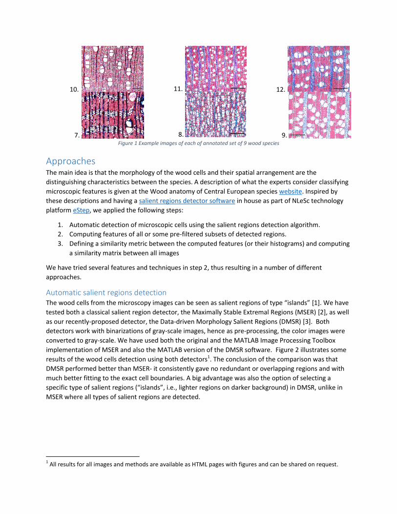
On Figure 1 the first image per specie are illustrated.

7. 8. 9.

10. 11. 12.

7. 8. 9. Figure 1 Example images of each of annotated set of 9 wood species

Approaches The main idea is that the morphology of the wood cells and their spatial arrangement are the

distinguishing characteristics between the species. A description of what the experts consider classifying

microscopic features is given at the Wood anatomy of Central European species website. Inspired by

these descriptions and having a salient regions detector software in house as part of NLeSc technology

platform eStep, we applied the following steps:

1. Automatic detection of microscopic cells using the salient regions detection algorithm.

2. Computing features of all or some pre-filtered subsets of detected regions.

3. Defining a similarity metric between the computed features (or their histograms) and computing

a similarity matrix between all images

We have tried several features and techniques in step 2, thus resulting in a number of different

approaches.

Automatic salient regions detection The wood cells from the microscopy images can be seen as salient regions of type “islands” [1]. We have

tested both a classical salient region detector, the Maximally Stable Extremal Regions (MSER) [2], as well

as our recently-proposed detector, the Data-driven Morphology Salient Regions (DMSR) [3]. Both

detectors work with binarizations of gray-scale images, hence as pre-processing, the color images were

converted to gray-scale. We have used both the original and the MATLAB Image Processing Toolbox

implementation of MSER and also the MATLAB version of the DMSR software. Figure 2 illustrates some

results of the wood cells detection using both detectors1. The conclusion of the comparison was that

DMSR performed better than MSER- it consistently gave no redundant or overlapping regions and with

much better fitting to the exact cell boundaries. A big advantage was also the option of selecting a

specific type of salient regions (“islands”, i.e., lighter regions on darker background) in DMSR, unlike in

MSER where all types of salient regions are detected.

1 All results for all images and methods are available as HTML pages with figures and can be shared on request.

Figure 2 Salient regions detection on the same wood images. The regions are shown by their equivalent ellipse representation.

Left: MSER original code (only every 3rd

region is shown); middle: MATLAB MSER implementation; right: DMSR

We have opted in using only DMSR regions for the rest of the experiments. An example of the exact

shaped regions (no their elliptic approximations) detected by DMSER is given on Figure 3.

Figure 3 Exact shape of the detected DMSR regions of type "islands" from a wood microscopy image.

Region features After the detection steps, we have computed various features of the individual salient regions.

Generic features for all regions

Basic region properties

The following properties were computed for all individual DMSR regions using the MATLAB Image

Processing Toolbox command regionprops: Area, Convex Area, Eccentricity, and Equivalent diameter,

Minor Axis Length, Major Axis Length and Orientation. For the exact definition of these properties,

please visit the regionprops web documentation. Histograms of the distribution of these properties for

all regions per image and for all images have been computed (see Figure 4).

Figure 4 Histograms of 7 properties of the detected DMSR regions from a wood microscopy image.

By inspecting these histograms, we concluded that not all of these basic properties are discriminative

enough across species and we opted for some derived and other more discriminative region properties.

Derived region properties

The selected 5 derived (or more discriminative basic) properties were:

1. Relative Area – the regions area divided by the image area and taking into account the

microscopy resolution (manually).

2. Eccentricity (as above) - the eccentricity of the ellipse that has the same second-moments as the

region. The eccentricity is the ratio of the distance between the foci of the ellipse and its major

axis length. (The value is between 0 and 1. An ellipse whose eccentricity is 0 is actually a circle,

while an ellipse whose eccentricity is 1 is a line segment.)

3. Orientation (as above) - the angle between the x-axis and the major axis of the ellipse that has

the same second-moments as the region. (The value is ranging from -90 to 90 degrees.)

4. RatioAxesLength- the ration of the Minor and Major Axis lengths (see above) of the ellipse that

has the same second-moments as the region.

5. Solidity - the proportion of the pixels in the convex hull that are also in the region. (Computed as

Area/ConvexArea. For details see regionprops web documentation).

As before, histograms of the distribution of these properties for all regions per image and for all images

have been computed (see Figure 5).

Figure 5 Histograms of 5 basic or derived properties of the detected DMSR regions from a wood microscopy image.

Features from groups of similar regions While the distributions of the generic features of all regions reflect the individual cell properties, one can

observe that the grouping of regions with certain properties into constellations is also characteristic of

some species. For instance, we can observe that the large round-shaped cells in Stemonurus celeb. are

evenly distributed across the tissue, while such regions come in clusters of 2 or 3 with Chrys afr. (see 9.

and 4. on Figure 1). Other examples are the elongated cells grouped in vertical “bands” for many species,

e.g. # 5, 6 and 9, while small round-shaped cells are grouped in vertical “ribbons” in Gluema ivor (7. on

Figure 1). These constellations (groups) are harder to automatically detect and describe in comparison

with the individual cell properties. We have opted for a 2 stage approach: firstly we filter similar regions

based on their individual properties (like Area, Eccentricity and Solidity) and next, we try to describe

their constellations.

Filtering of similar regions

We have defined 4 groups of regions, we would like to detect and have (manually) defined a filtering

criteria:

Regions description Filtering condition

Large Big Relative Area ([0.2, 1]) AND big Solidity ([0.85, 1])

Small Small Relative Area ([0, 0.199]) AND big Solidity ([0.85, 1])

Small round-shaped horizontally oriented

Small Eccentricity ([0, 0.85]) AND big Solidity ([0.85, 1]) AND small Relative Area ([0, 0.199])

Small elongated vertically oriented

Vertical Orientation ([-90,-55] OR [55, 90]) AND big Eccentricity ([0.75,1]) AND small Relative Area ([0,0.2])

We have filtered the above 4 types of regions for every image using the binary masks of all salient

regions obtained by the DMSR detector. An illustration of the filtering of the large round-shaped regions

can be seen on Figure 6 and of the small elongated vertically oriented ones - on Figure 7.

Figure 6 Large DMSR regions filtered from all regions from a wood microscopy image.

Figure 7 Small vertical elongated DMSR regions filtered from all regions from a wood microscopy image.

Features for regions groups After obtaining the 4 types of regions by filtering we have tried 2 approaches for constructing

discriminating features of the constellation of the filtered regions.

DBSCAN clustering

The Density-based spatial clustering of applications with noise (DBSCAN) is one of the most common

clustering algorithms and also most cited in scientific literature. Given a set of points in some space, it

groups together points that are grouped together (points with many nearby neighbors), marking as noise

(outliers) points that lie alone in low-density regions (whose nearest neighbors are too far away). In our

problem we considered the centroids of each region as the set of points to be clustered. DBSCAN

requires two parameters: ε - the distance between 2 points to be considered neighbors and minPts -the

minimum number of points required to form a dense region. We have used the open-source MATLAB

implementation of DBSCAN from yarpiz on the set of centroids of each filtered image using minPts = 2

and 3 different distances , where , l is the image diagonal length

and is the microscopic resolution. The DBSCAN algorithm on the Chrys afr image from Figure 6 is

shown on Figure 8.

Figure 8 DBSCAN clusters of large salient regions’ centroids with increasing distance between neighboring points .

To describe the constellations of regions via these clusters we have constructed a vector of elements per

cluster vector (EPCV) and have defined a number of quantitative features:

1. Total number of clusters

2. Number of elements in cluster ‘noise’

3. Maximum of the EPCV

4. Minimum of the EPCV

5. Mean of the EPCV

6. Standard deviation of the EPCV

Therefore, we obtain an 18 (3*6)-dimensional feature vector per filtered version of every image (e.g.

would sum up to 4 features vectors per wood image in total). The graphs on Figure 9 illustrate these

features for the filtered large salient regions masks for 2 species (2 images per specie). We can see that

these vectors are very similar for species that have more clusters of large regions (e.g. 8. Rhaptop), while

are not so useful for species that don’t (e.g. 7.Gluema). Therefore we decided to abandon this approach.

Figure 9 Features of DBSCAN clusters of large salient regions' centroids for 2 species of wood.

Successive morphological dilations

Another approach for describing the constellations of regions is to use successive dilations. The

morphological dilation operation with a structuring element (SE) "expands" the boundaries of a region

with pixels determined by the geometry of the SE we used a disk with radius r. Successive dilations of a

binary mask is given on Figure 10.

Figure 10 Successive morphological dilations (3 iterations) of the binary mask of large salient regions for Argania.

Since the number of regions after each dilation will be the same or smaller, a vector with all iteration

number of regions counts is the feature to describe the successive dilations. We have experimented with

two options for the SE radius:

Fixed:

Adaptive: , where is the mean equivalent diameter (diameter of a circle with the

same area as the region) for all regions.

The vector of counts for the number of regions dilated with an adaptive SE for the 2 images of

Stemonurus celebicus are illustrated on Figure 11.

Figure 11 Number of regions for 10 iterations of successive dilations on the 4 types of filtered regions for Stemonurus celebicus.

We have observed that these vectors look similar for the same species and different for images of different species.

Similarity metrics The final step after the automatic region detection and constructing features describing the spatial

arrangement (constellation) of the regions is the similarity between the features. We have considered

similarity for 2 types of features: histograms of individual derived region properties (see Derived region

properties) and constellation features obtained via successive dilations (see Successive morphological

dilations).

Similarity metrics on derived properties for all regions As described in Derived region properties we have considered the histograms of 4 (Solidity was not used)

derived properties of all regions: RelativeArea, Eccentricity, Orientation and RatioAxesLength. We have

tested 7 distance metrics between these histograms:

1. Chi-squared statistics

2. Histogram intersection

3. Kolmogorov- Smirnov distance

4. Kullback-Leibler divergence

5. Jeffrey divergence

6. Jensen-Shannon divergence

7. Match distance

The experiments showed that metrics 4, 5 and 6 were not suitable to measure similarity (1 – distance)

for these data. The match distance achieved the best similarity matrix, but none of the features alone

seem to provide the proper classification, though correct patterns emerge (see Figure 12).

Figure 12 Similarity matrix between histograms of derived features for all data using match distance metric.

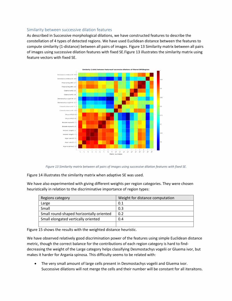
Similarity between successive dilation features As described in Successive morphological dilations, we have constructed features to describe the

constellation of 4 types of detected regions. We have used Euclidean distance between the features to

compute similarity (1-distance) between all pairs of images. Figure 13 Similarity matrix between all pairs

of images using successive dilation features with fixed SE.Figure 13 illustrates the similarity matrix using

feature vectors with fixed SE.

Figure 13 Similarity matrix between all pairs of images using successive dilation features with fixed SE.

Figure 14 illustrates the similarity matrix when adaptive SE was used.

We have also experimented with giving different weights per region categories. They were chosen

heuristically in relation to the discriminative importance of region types:

Regions category Weight for distance computation

Large 0.1

Small 0.3

Small round-shaped horizontally oriented 0.2

Small elongated vertically oriented 0.4

Figure 15 shows the results with the weighted distance heuristic.

We have observed relatively good discrimination power of the features using simple Euclidean distance

metric, though the correct balance for the contributions of each region category is hard to find-

decreasing the weight of the Large category helps classifying Desmostachys vogelii or Gluema ivor, but

makes it harder for Argania spinosa. This difficulty seems to be related with:

The very small amount of large cells present in Desmostachys vogelii and Gluema ivor.

Successive dilations will not merge the cells and their number will be constant for all iteraitons.

The difference in resolution in Desm. vog. images results in different Large cell counts and hence

smaller impact of that category.

Figure 14 Similarity matrix between all pairs of images using successive dilation features with adaptive SE.

Figure 15 Similarity matrix between all pairs of images using successive dilation features with adaptive SE and weighted distance metric.

Conclusions We have demonstrated on a small annotated dataset of wood microscopy images that it is possible to:

1. Automatically extract the cells using our generic salient regions software.

2. Filter the cells based on their individual properties such as RelativeArea, Eccentricity, Orientation

and Solidity.

3. Construct region features from the extracted regions both based on individual characteristics as

well as on constellations of the regions.

4. Define similarity metric on the features which are able to distinguish between most of the

present species. It is sometimes hard to find the best balance of the generic features due to the

different nature of the wood cells and their distribution for the different species.

This document describes the methods and presents some promising initial results. Much more

annotated data and more research is needed to answer the research questions.

References

[1] E. Ranguelova and E. Pauwels, "Morphology-based Stable Salient Regions Detector," in International

conference on Image and Vision Computing New Zealand (IVCNZ’06), 2006.

[2] J. Matas, O. Chum, M. Urban and T. Pajdla, "Robust Wide Baseline Stereo from Maximally Stable

Extremal Regions," in British Machine Vision Conference (BMVC), 2002.

[3] E. Ranguelova, "A Data-driven Region Detector for Structured Image Scenes," in International

Conference on Image Processing (ICIP'16), submitted, under revision, 2016.