Elena Pavelescu- Braids and Open Book Decompositions
66
BRAIDS AND OPEN BOOK DECOMPOSITIONS Elena Pavelescu A Dissertation in Mathematics Presented to the Faculties of the University of Pennsylvania in Partial Fulfillment of the Requirements for the Degree of Doctor of Philosophy 2008 John Etnyre Supervisor of Dissertation Tony Pantev Graduate Group Chairperson
Transcript of Elena Pavelescu- Braids and Open Book Decompositions

8/3/2019 Elena Pavelescu- Braids and Open Book Decompositions
http://slidepdf.com/reader/full/elena-pavelescu-braids-and-open-book-decompositions 1/66
BRAIDS AND OPEN BOOK DECOMPOSITIONS
Elena Pavelescu
A Dissertation
in
Mathematics
Presented to the Faculties of the University of Pennsylvania in Partial
Fulfillment of the Requirements for the Degree of Doctor of Philosophy
2008
John EtnyreSupervisor of Dissertation
Tony PantevGraduate Group Chairperson

8/3/2019 Elena Pavelescu- Braids and Open Book Decompositions
http://slidepdf.com/reader/full/elena-pavelescu-braids-and-open-book-decompositions 2/66
To Andrei and my parents
ii

8/3/2019 Elena Pavelescu- Braids and Open Book Decompositions
http://slidepdf.com/reader/full/elena-pavelescu-braids-and-open-book-decompositions 3/66
Acknowledgments
First and foremost I would like to thank my advisor, John Etnyre, for all his support
during the last years. Your constant encouragements and contagious optimism kept
me going. Thank you for everything!
I would also like to thank Herman Gluck, Paul Melvin and Rafal Komedarczyk
for their time and interest in my work and Florian Pop for being part of my thesis
defense committee.
A special thanks to the four persons who keep the mathematics department run-
ning: Janet Burns, Monica Pallanti, Paula Scarborough and Robin Toney. Thank
you for always being available and kind.
I want to thank Alina Badus. and John Parejko, Sarah Carr, Enka Lakuriqi and
Jimmy Dillies, Vittorio Perduca, John Olsen, Tomoko Shibuya and Meesue Yoo for
their friendship and for all the great postcards.
I am most grateful to my parents, Elena and Mircea Bogdan, and to the rest of
my family who have always believed in me and offered me their constant support.
My thoughts go to Cri, whom I miss terribly.
iii

8/3/2019 Elena Pavelescu- Braids and Open Book Decompositions
http://slidepdf.com/reader/full/elena-pavelescu-braids-and-open-book-decompositions 4/66
Finally, I want to thank my husband, Andrei Pavelescu. Thank you for all your
love and kindness, I couldn’t have made it without you.
iv

8/3/2019 Elena Pavelescu- Braids and Open Book Decompositions
http://slidepdf.com/reader/full/elena-pavelescu-braids-and-open-book-decompositions 5/66
ABSTRACT
BRAIDS AND OPEN BOOK DECOMPOSITIONS
Elena Pavelescu
John Etnyre, Advisor
In this thesis we generalize Alexander’s and Bennequin’s work on braiding knots
and Markov’s theorem about when two braids represent isotopic knots. We also
reprove Eliashberg’s theorem on the transversal simplicity of the unknot in a tight
contact structure using braid theoretical techniques. Finally, we look at possible
changes in braid foliations induced on a surface.
v

8/3/2019 Elena Pavelescu- Braids and Open Book Decompositions
http://slidepdf.com/reader/full/elena-pavelescu-braids-and-open-book-decompositions 6/66
Contents
1 Introduction 3
2 Background 5
2.1 Contact structures . . . . . . . . . . . . . . . . . . . . . . . . . . . 5
2.2 Gray’s theorem . . . . . . . . . . . . . . . . . . . . . . . . . . . . . 7
2.3 Transverse and Legendrian arcs . . . . . . . . . . . . . . . . . . . . 9
2.4 Open book decompositions . . . . . . . . . . . . . . . . . . . . . . . 10
3 The generalized Alexander theorem 16
3.1 Preliminaries . . . . . . . . . . . . . . . . . . . . . . . . . . . . . . 16
3.2 The generalized Alexander theorem . . . . . . . . . . . . . . . . . . 18
4 The generalized Markov theorem 24
4.1 Geometric Markov theorem in an open book decomposition . . . . . 24
4.2 The standard braid group and Markov moves . . . . . . . . . . . . 27
4.3 Braids in an open book decomposition . . . . . . . . . . . . . . . . 28
vi
8/3/2019 Elena Pavelescu- Braids and Open Book Decompositions
http://slidepdf.com/reader/full/elena-pavelescu-braids-and-open-book-decompositions 7/66
4.4 Algebraic interpretation of the Markov theorem in an open book
decomposition . . . . . . . . . . . . . . . . . . . . . . . . . . . . . . 31
5 On the transversal simplicity of the unknot 36
5.1 Braid foliations . . . . . . . . . . . . . . . . . . . . . . . . . . . . . 37
5.2 Transverse stabilizations and braid destabilizations . . . . . . . . . 43
5.3 In a tight contact structure the unknot is transversely simple . . . . 47
6 Surface changes 52
6.1 Few preliminaries . . . . . . . . . . . . . . . . . . . . . . . . . . . . 52
6.2 Changing order of adjacent saddle points . . . . . . . . . . . . . . . 53
vii

8/3/2019 Elena Pavelescu- Braids and Open Book Decompositions
http://slidepdf.com/reader/full/elena-pavelescu-braids-and-open-book-decompositions 8/66
List of Figures
2.1 (a) h function (b) g function . . . . . . . . . . . . . . . . . . . . . . . 14
3.1 Wrinkling along a bad arc γ . . . . . . . . . . . . . . . . . . . . . . . . 17
3.2 Transforming a non-shadowed bad arc into a good arc. . . . . . . . . . 18
3.3 Wrinkling K in order to avoid intersections with S . . . . . . . . . . . 23
4.1 Wrinkling in order to avoid intersections between B and S . . . . . . . 26
4.2 (a) Braids representing σi and σ−1i (b) Positive Markov move . . . . . . 28
4.3 Generators of the braid group of a surface. . . . . . . . . . . . . . . . . 30
4.4 Stabilization about a second binding component . . . . . . . . . . . . . 34
5.1 (a) Homotopically trivial γ (b) Homologically trivial γ not bounding a
disk (c) Homologically essential γ . . . . . . . . . . . . . . . . . . . . 40
5.2 (a,b)Positive and negative elliptic singularities (c,d) Positive and negative
hyperbolic singularities . . . . . . . . . . . . . . . . . . . . . . . . . . 41
5.3 Induced braid foliation on D. . . . . . . . . . . . . . . . . . . . . . . 42
1

8/3/2019 Elena Pavelescu- Braids and Open Book Decompositions
http://slidepdf.com/reader/full/elena-pavelescu-braids-and-open-book-decompositions 9/66
5.4 Part of D before and after the elimination of a negative hyperbolic singu-
larity adjacent to U . . . . . . . . . . . . . . . . . . . . . . . . . . . . 45
5.5 (a) Disk foliation of complexity 1 (b) Valence 1 elements in E U (c) Stabi-
lization disk . . . . . . . . . . . . . . . . . . . . . . . . . . . . . . . 46
5.6 Isotopy between trivial unknots linking different binding components. . . 49
5.7 Arc isotopy from one binding component to another. . . . . . . . . . . 51
6.1 Possible tiles in the decompositions of S . . . . . . . . . . . . . . . . . . 53
6.2 Neighborhood of adjacent saddle points of the same sign before and after
the isotopy. . . . . . . . . . . . . . . . . . . . . . . . . . . . . . . . . 54
6.3 Traces of a neighborhood of adjacent saddle points of the same sign on
different Σθ’s. . . . . . . . . . . . . . . . . . . . . . . . . . . . . . . . 56
2

8/3/2019 Elena Pavelescu- Braids and Open Book Decompositions
http://slidepdf.com/reader/full/elena-pavelescu-braids-and-open-book-decompositions 10/66
Chapter 1
Introduction
In [2], Alexander proved that any knot in R3 can be braided about the z-axis.
In [6], a paper which marked the start of modern contact topology, leading to
the Bennequin inequality and the definition of tightness, Bennequin proved the
transverse case for (R3, ξstd). Following a review of known results and background
material, in Chapter 3 we generalize Bennequin’s result to any closed, oriented, 3-
dimensional manifold M , by looking at an open book decomposition for M together
with a supported contact structure.
In [17], Markov gave an equivalent condition for two braids in R3 to be isotopic.
This is the case if and only if the two braids differ by conjugations in the braid group
and positive and negative Markov moves. In [18] Orevkov and Shevchishin proved
the transversal case for (R3, ξstd). A different proof was independently obtained
by Wrinkle in [23]. In Chapter 4 we generalize Markov’s theorem to any closed,
3

8/3/2019 Elena Pavelescu- Braids and Open Book Decompositions
http://slidepdf.com/reader/full/elena-pavelescu-braids-and-open-book-decompositions 11/66
oriented, 3-dimensional manifold. We prove the transverse case and recover the
topological case previously proved in [20] and [21].
In [10], Birman and Wrinkle proved that exchange reducibility implies transversal
simplicity. As a consequence, Birman and Menasco’s paper [8] shows that the
m-component unlink is transversely simple. While exchange reducibility does not
seam to work in more general settings, the unknot remains transversely simple in
a tight contact structure. Eliashberg proved this fact in [11]. Later, Etnyre ([14])
proved that positive torus knots are transversely simple. In Chapter 5 we reprove
Eliashberg’s original result using braid theoretical techniques.
In Chapter 6 we look closer at foliations induced on an embedded surface S ⊂ M 3
by the intersection with the pages of an open book decomposition (Σ, φ) for M 3 and
we show how adjacent saddle points can be changed with respect to the coordinate
on S 1, generalizing a result of Birman and Menasco ([8]). .
4
8/3/2019 Elena Pavelescu- Braids and Open Book Decompositions
http://slidepdf.com/reader/full/elena-pavelescu-braids-and-open-book-decompositions 12/66
Chapter 2
Background
In this chapter we review some of the definitions and results that we’ll be using
throughout this thesis.
2.1 Contact structures
Definition 2.1.1. Let M be a compact, oriented 3-manifold and ξ a subbundle of
the tangent bundle of M such that ξ p = T pM ∩ ξ is a two dimensional subspace of
T pM for all p ∈ M . Locally, ξ can be written as ξ = ker α for some non-degenerate
1-form α. The plane field ξ is called a contact structure if α ∧ dα = 0.
Such a plane field is completely non-integrable, that is ξ is not tangent to any
surface along an open set. If ξ is orientable, then it can be written as ξ = ker α for
a global 1-form α. Depending on whether α ∧ dα > 0 or α ∧ dα < 0, ξ is called
a positive or a negative contact structure. The contact structures we are working
5

8/3/2019 Elena Pavelescu- Braids and Open Book Decompositions
http://slidepdf.com/reader/full/elena-pavelescu-braids-and-open-book-decompositions 13/66
with throughout this paper are assumed to be oriented and positive.
Definition 2.1.2. A contactomorphism between two contact manifolds (M 1, ξ1)
and (M 2, ξ2) is a diffeomorphism φ : M 1 → M 2 such that φ∗ξ1 = ξ2.
Definition 2.1.3. An embedded disk D in (M, ξ) is called an overtwisted disk if
T p∂D ⊂ ξ for all p ∈ ∂D and D is transverse to ξ along ∂D. If there exists such a
disk in (M, ξ) then ξ is called overtwisted . If it is not overtwisted a contact structure
is called tight .
On R3, consider the two contact structures ξ1 and ξ2 given by the 1-forms
α1 = dz − ydx and α2 = dz + r2dθ (given in cylindrical coordinates). These two
contact structures are contactomorphic and we are going to refer to them as the
standard contact structure, ξstd.
Unlike Riemannian geometry, contact geometry doesn’t exhibit any special local
behavior, as we can see from the following theorem.
Theorem 2.1.4. (Darboux) Let (M, ξ) be a contact manifold. Every point p ∈
M has a neighborhood that is contactomorphic to a neighborhood of the origin in
(R3, ξstd).
A proof of this theorem can be found in [1].
Definition 2.1.5. The Reeb vector field of α is the unique vector field vα on M
such that
i) α(vα) = 1
6
8/3/2019 Elena Pavelescu- Braids and Open Book Decompositions
http://slidepdf.com/reader/full/elena-pavelescu-braids-and-open-book-decompositions 14/66
ii) dα(vα, ·) = 0
Definition 2.1.6. Let Σ ⊂ (M, ξ) be an embedded surface. From the non-integrability
condition of ξ it follows that lx = T xΣ ∩ ξx is a line for most points x ∈ Σ. The
singular foliation on Σ whose leaves are tangent to the line field l = ∪lx is called
the characteristic foliation of Σ.
The characteristic foliation of a surface Σ determines a whole neighborhood of
Σ as follows from the next theorem.
Theorem 2.1.7. If Σi ⊂ (M i, ξi), for i = 1, 2 are two embedded surfaces and there
exists a diffeomorphism f : Σ1 → Σ2 which preserves the characteristic foliations
then f may be isotoped to be a contactomorphism in a neighborhood of Σ1.
2.2 Gray’s theorem
The following theorem is of vital importance in proving the generalization of Alexan-
der’s theorem on braiding links (Chapter 3).
Theorem 2.2.1. ( Gray ) Let ξtt∈[0,1] be a family of contact structures on a
manifold M that differ on a compact set C ⊂ int (M ). Then there exists an isotopy
ψt : M → M such that
i) (ψt)∗ξ0=ξt
ii) ψt is the identity outside of an open neighborhood of C .
7
8/3/2019 Elena Pavelescu- Braids and Open Book Decompositions
http://slidepdf.com/reader/full/elena-pavelescu-braids-and-open-book-decompositions 15/66
Proof. We are going to look for ψt as the flow of a vector field X t. If ξt = ker αt,
then ψt has to satisfy
ψ∗
t αt = λtα0, (2.2.1)
for some non-vanishing function λt : M → R3. By taking the derivative with re-
spect to t on both sides the equality will still hold. Thus,
d
dt(ψ∗
t αt) = limh→0
ψ∗t+hαt+h − ψ∗
t αt
h= lim
h→0
ψ∗t+hαt+h − ψ∗
t+hαt + ψ∗t+hαt − ψ∗
t αt
h=
= ψ∗
t (dαt
dt) + ψ∗
t LXtαt = ψ∗
t (dαt
dt+ LXtαt).
This gives
ψ∗
t (dαt
dt+ LXtαt) =
dλt
dtα0 =
dλt
dt
1
λtψ∗αt (2.2.2)
and by letting
ht =d
dt(log λt) ψ−1
t (2.2.3)
we get
ψ∗
t (dαt
dt+ d(ιXtαt) + ιXtdαt) = ψ∗
t (htαt) (2.2.4)
If X t is chosen in ξt then ιXtαt = 0 and the last equality becomes
dαt
dt+ ιXtdαt = htαt (2.2.5)
Applying (2.2.5) to the Reeb vector field of αt, vαt, we find ht = dαtdt (vαt) and have
8

8/3/2019 Elena Pavelescu- Braids and Open Book Decompositions
http://slidepdf.com/reader/full/elena-pavelescu-braids-and-open-book-decompositions 16/66
the following equation for X t
ιXtdαt = htαt −dαt
dt(2.2.6)
The form dαt gives an isomorphism
Γ(ξt) → Ω1αt
v → ιvdαt
Where Γ(ξt) = v|v ∈ ξt and Ω1αt = 1-forms β |β (vt) = 0. This implies that X t
is uniquely determined by (2.2.6) and by construction the flow of X t works.
For the subset of M where the ξt’s agree we just choose the αt’s to agree. This
implies dαtdt
= 0, ht = 0 and X t = 0 and all equalities hold.
2.3 Transverse and Legendrian arcs
Definition 2.3.1. In a contact manifold (M, ξ), an oriented arc γ ⊂ M is called
transverse if for all p ∈ γ and ξ p the contact plane at p, T pγ ξ p and T pγ points
towards the positive normal direction of the oriented plane ξ p. If γ is a closed curve
then it is called a transverse knot .
Definition 2.3.2. In a contact manifold (M, ξ), an arc γ ⊂ M is called Legendrian
if for all p ∈ γ , T pγ ⊂ ξ p, where ξ p is the contact plane at p. If γ is a closed curve
then it is called a Legendrian knot .
Around a transversal (or Legendrian) knot contact structures always look the
same. Using Theorem 2.2.1 we can prove the following two lemmas.
9
8/3/2019 Elena Pavelescu- Braids and Open Book Decompositions
http://slidepdf.com/reader/full/elena-pavelescu-braids-and-open-book-decompositions 17/66
Lemma 2.3.3. A neighborhood of a transverse knot in any contact manifold is
contactomorphic with a neighborhood of the z-axis in (R3, ξstd)/z∼z+1.
Lemma 2.3.4. A neighborhood of a Legendrian knot in any contact manifold is
contactomorphic with a neighborhood of the x-axis in (R3, ξstd)/x∼x+1.
Definition 2.3.5. Let K ⊂ (M, ξ) be a null homologous knot and Σ ⊂ M a surface
such that ∂ Σ = K . Let v ∈ ξ|∂ Σ be the restriction to K of a non-zero vector field
w ∈ ξ on Σ. Denote by K the push-off of K in the direction of v. The self-linking
number of K is sl(K ) = lk(K, K
) = K
· Σ (algebraic intersection).
2.4 Open book decompositions
Definition 2.4.1. An open book decomposition of M is a pair (L, π) where
i) L is an oriented link in M called the binding of the open book
ii) π : M L → S 1 is a fibration whose fiber, π−1(θ), is the interior of a compact
surface Σ ⊂ M such that ∂ Σ = L, ∀θ ∈ S 1. The surface Σ is called the page
of the open book.
Alternatively, an open book decomposition of a 3-manifold M consists of a
surface Σ, with boundary, together with a diffeomorphism φ : Σ → Σ, with φ=
identity near ∂ Σ, such that
M = (Σ × [0, 1]/ ∼) ∪f
i
S 1 × D2
10

8/3/2019 Elena Pavelescu- Braids and Open Book Decompositions
http://slidepdf.com/reader/full/elena-pavelescu-braids-and-open-book-decompositions 18/66
where
(x, 1) ∼ (φ(x), 0).
Note that
∂ (Σ × [0, 1]/ ∼) =
i
T 2i ,
each torus T 2i having a product structure S 1 × [0, 1]/ ∼. Let λi = pt × [0, 1]/ ∼,
λi ∈ T 2i . The gluing diffeomorphism used to construct M is defined as
f : ∂ (
i
S 1 × D2) → ∂ (
i
T 2i )
pt × ∂D2 → λi.
The map φ is called the monodromy of the open book.
Theorem 2.4.2. (Alexander, [3]) Every closed oriented 3-manifold has an open
book decomposition.
Definition 2.4.3. A contact structure ξ on M is said to be supported by an open
book decomposition (Σ, φ) of M if ξ can be isotoped through contact structures so
that there exists a 1-form α for ξ such that
i) dα is a positive area form on each page
ii) α(v) > 0 for all v ∈ T L that induce the orientation on L.
11

8/3/2019 Elena Pavelescu- Braids and Open Book Decompositions
http://slidepdf.com/reader/full/elena-pavelescu-braids-and-open-book-decompositions 19/66
Lemma 2.4.4. A contact structure ξ on M is supported by an open book decom-
position (Σ, φ) if and only if (Σ, φ) is an open book decomposition of M and ξ can
be isotoped to be arbitrarily close, as oriented plane fields, on compact subsets of
the pages, to the tangent planes to the pages of the open book in such a way that
after some point in the isotopy the contact planes are transverse to the binding and
transverse to the pages in a neighborhood of the binding.
Contact structures and open book decompositions are closely related. Thurston
and Winkelnkemper have shown how to get contact structures from open books.
Theorem 2.4.5. (Thurston, Winkelnkemper, [22]) Every open book decomposition
(Σ, φ) supports a contact structure ξφ.
Proof. Let
M = (Σ × [0, 1]/ ∼) ∪f
i
S 1 × D2
given as before. We first construct a contact structure on Σ × [0, 1]/ ∼ and then we
extended it in a neighborhood of the binding. Let (ψ,x,θ) be coordinates near each
of the binding components ((ψ, x) are coordinates on the page, with ψ being the
coordinate along the binding, while θ is the coordinate pointing out of the page)
and consider the set of forms
S = 1 − forms λ such that : dλ is a volume form on Σ
λ = (1 + x)dψ near ∂ Σ = L
To show that the set S is non-empty let λ1 be a 1-form on Σ such that λ1 = (1+x)dψ
12

8/3/2019 Elena Pavelescu- Braids and Open Book Decompositions
http://slidepdf.com/reader/full/elena-pavelescu-braids-and-open-book-decompositions 20/66
near ∂ Σ. Let ω be a volume form on Σ such that ω = dx ∧ dψ near ∂ Σ. The form
ω−dλ1 is closed and since H 2(Σ) = 0, there exists a 1-form β such that dβ = ω−dλ1
and β = 0 near ∂ Σ. Then λ = λ1 + β is an element in S .
Note that for λ ∈ S , then φ∗λ is also in S .
Let λ be an element of S and consider the 1-form
λ( p,t) = tλ p + (1 − t)(φ∗λ) p
on Σ × [0, 1] where ( p,t) ∈ Σ × [0, 1] and take
αK = λ( p,t) + Kdt.
For sufficiently large K , αK is a contact form and it descends to a contact form on
Σ × [0, 1]/ ∼. We want to extend this form on the solid tori neighborhood of the
binding. Consider coordinates (ψ,r,θ) in a neighborhood S 1 × D2 of each binding
component. The gluing map f is given by
f (ψ,r,θ) = (r − 1 + , −ψ, θ).
Pulling back the contact form αK through this map gives the 1-form
αf = Kdθ − (r + )dψ.
We are looking to extend this form on the entire S 1 × D2 to a contact form of the
form h(r)dψ + g(r)dθ. This is possible if there exist functions h, g : [0, 1] → R3 such
that:
i) h(r)g(r) − h(r)g(r) > 0 (given by the contact condition)
13

8/3/2019 Elena Pavelescu- Braids and Open Book Decompositions
http://slidepdf.com/reader/full/elena-pavelescu-braids-and-open-book-decompositions 21/66
ii) h(r) = 1 near r = 0, h(r) = −(r + ) near r = 1
iii) g(r) = r2 near r = 0, g(r) = K near r = 1.
h
δh
−1 −
1
1
r
(a)
g
δg
K
1
1
r
(b)
Figure 2.1: (a) h function (b) g function
The two functions h and g described in Figure 2.1 work for our purpose. The
conditions i) and ii) are obviously satisfied and if δh and δg are such that h < 0 on
[δh, 1] and g = 1 on [δg, 1], then iii) is satisfied as long as δh < δg.
In [15], Giroux proved there exists a correspondence between contact structures
and open book decompositions.
Theorem 2.4.6. (Giroux) Let M be a closed, oriented 3-manifold. Then there is a
one to one correspondence between oriented contact structures on M up to isotopy
and open book decompositions of M up to positive stabilizations.
Definition 2.4.7. A positive (negative) stabilization of an open book (Σ, φ) is the
open book with
14

8/3/2019 Elena Pavelescu- Braids and Open Book Decompositions
http://slidepdf.com/reader/full/elena-pavelescu-braids-and-open-book-decompositions 22/66
i) page Σ = Σ ∪ 1 − handle
ii) monodromy φ = φ τ c, where τ c is a right-(left-)handed Dehn twist along a
curve c in Σ
that runs along the added 1-handle exactly once.
15

8/3/2019 Elena Pavelescu- Braids and Open Book Decompositions
http://slidepdf.com/reader/full/elena-pavelescu-braids-and-open-book-decompositions 23/66
Chapter 3
The generalized Alexander
theorem
3.1 Preliminaries
In [2], Alexander proved that any link in R3
can be isotoped to a link braided about
the z-axis. In [6] Bennequin proved the transverse case, that is that any transverse
link in (R3, ξstd) can be transversely braided about the z-axis. The goal of this
chapter is to prove a generalization of Bennequin’s result. Throughout this section
M is a closed and oriented 3-manifold.
Definition 3.1.1. Let (L, π) be an open book decomposition for M . A link K ⊂ M
is said to be braided about L if K is disjoint from L and there exists a parametrization
of K , f :
S 1 → M such that if t is the coordinate on each S 1 then ddt
(π f ) > 0
16

8/3/2019 Elena Pavelescu- Braids and Open Book Decompositions
http://slidepdf.com/reader/full/elena-pavelescu-braids-and-open-book-decompositions 24/66
at all time.
Our proof reduces the general case to the (R3, ξstd) case proved by Bennequin.
Below we sketch the ideas he used in his proof.
Theorem 3.1.2. (Bennequin, [6]) Any transverse link Γ in (R3, ξstd) is transversely
isotopic to a link braided about the z-axis.
Proof. Let (r,θ,z) be cylindrical coordinates on R3 and let t be the parameter on
Γ. The standard contact structure is given by α = dz + r2dθ. The arcs constituting
Γ are either good (if dθdt > 0 ) or bad (if dθ
dt≤ 0). In order to arrange Γ into a braid
form, the bad arcs are moved through a transverse isotopy on the other side of the
z-axis. This requires that certain wrinklings, which we describe below, are done
along the bad arcs. Along a bad arc γ ⊂ Γ we have dθdt
< 0 and dzdt
> 0, as the
knot is transverse. The projection of γ on a large enough r−cylinder looks like the
one in Figure 3.1. The wrinkling leaves the r coordinate unchanged and modifies
the z and θ coordinates. As throughout the wrinkling dzdθ
increases and r remains
constant, the arc remains transverse to the contact planes. An arc γ ⊂ Γ is said
zz
θθ
γ
γ
Figure 3.1: Wrinkling along a bad arc γ .
17
8/3/2019 Elena Pavelescu- Braids and Open Book Decompositions
http://slidepdf.com/reader/full/elena-pavelescu-braids-and-open-book-decompositions 25/66
to be shadowed by another arc γ at (r,θ,z) ∈ γ if there exists (r, θ , z) ∈ γ with
r < r.
i) By introducing a wrinkle as in Figure 3.1 on the bad arc γ , it can be arranged
that γ doesn’t go all around the z-axis.
ii) By introducing a wrinkle as in Figure 3.1 on the bad arc γ , it can be arranged
that γ is not shadowed by any other arc.
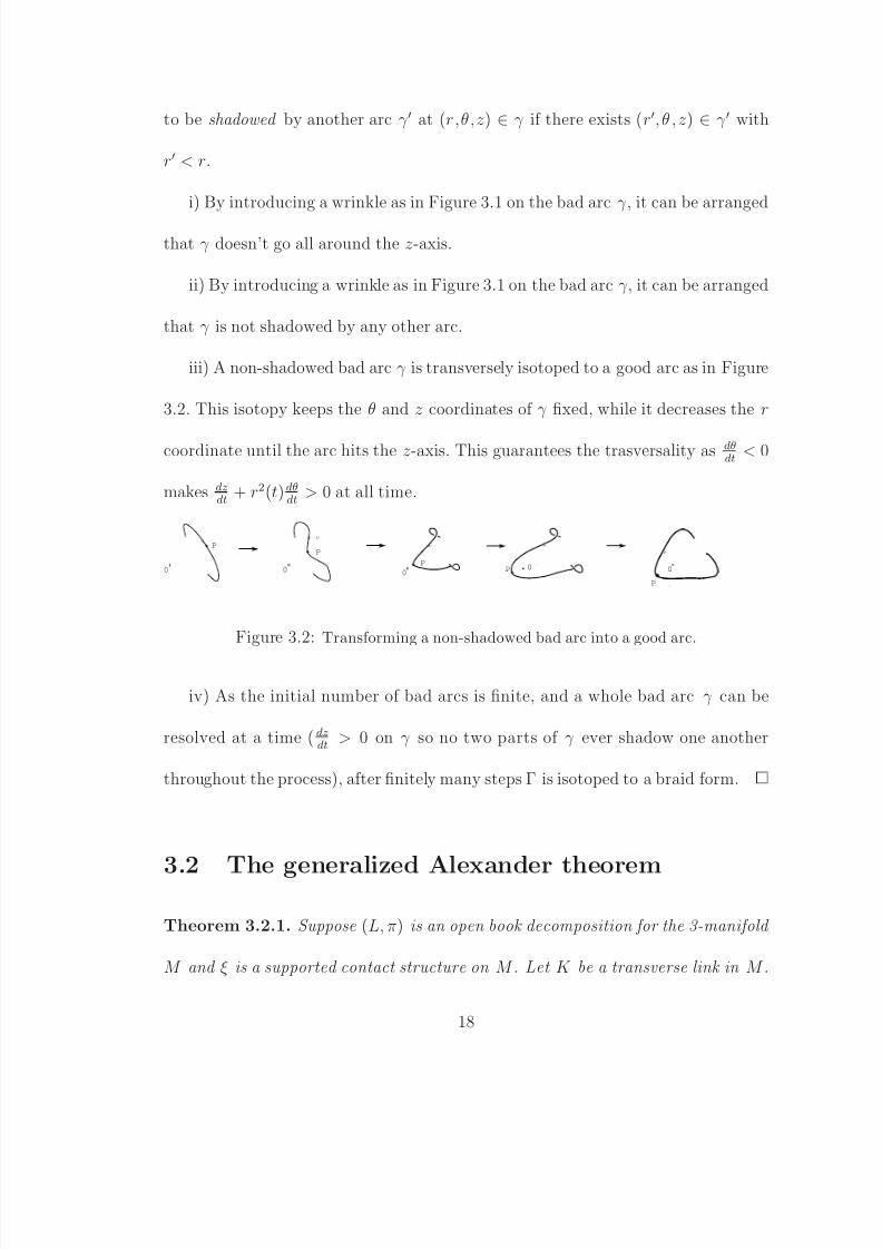
iii) A non-shadowed bad arc γ is transversely isotoped to a good arc as in Figure
3.2. This isotopy keeps the θ and z coordinates of γ fixed, while it decreases the r
coordinate until the arc hits the z-axis. This guarantees the trasversality as dθdt
< 0
makes dzdt
+ r2(t) dθdt
> 0 at all time.
0
>
P
0
>
P
P
> >
P
>
P
>
0 00
Figure 3.2: Transforming a non-shadowed bad arc into a good arc.
iv) As the initial number of bad arcs is finite, and a whole bad arc γ can be
resolved at a time ( dzdt > 0 on γ so no two parts of γ ever shadow one another
throughout the process), after finitely many steps Γ is isotoped to a braid form.
3.2 The generalized Alexander theorem
Theorem 3.2.1. Suppose (L, π) is an open book decomposition for the 3-manifold
M and ξ is a supported contact structure on M . Let K be a transverse link in M .
18

8/3/2019 Elena Pavelescu- Braids and Open Book Decompositions
http://slidepdf.com/reader/full/elena-pavelescu-braids-and-open-book-decompositions 26/66
Then K can be transversely isotoped to a braid.
Proof. The idea of the proof is to find a family of diffeomorphisms of M keeping
each page of the open book setwise fixed and taking the parts of the link where
the link is not braided in a neighborhood of the binding. A neighborhood of the
binding is contactomorphic to a neighborhood of the z-axis in (R3, ξstd)/z∼z+1 and
there the link can be braided, according to Theorem 3.1.2.
In the neighborhood N = S 1 × D2 of each component of the binding consider
coordinates (ψ,x,θ) such that dθ and π∗dθ agree, where π∗dθ is the pullback through
π : M \ L → S 1 of the coordinate on S 1.
As ξ is supported by the open book (L, π), ξ can be isotoped to a contact
structure ξ that is arbitrarily close to being tangent to the pages of the open book.
Consider a 1-form λ on Σ such as in Lemma 2.4.5. On Σ × [0, 1] take λ =
(1 − θ)λ + θ(φ∗λ) and consider the family of 1-forms given by αt = λ + K 1t
dθ, where
t ∈ (0, 1] and K is any large constant. This family of 1-forms descends to a family
of 1-forms on Σ × [0, 1]/ ∼.
Both ξ1 = ker(α1) and ξ are contact structures supported by (L, π) and so they
are isotopic. Therefore, without loosing generality, we may assume ξ = ker(α1).
Note that for t → 0, αt defines a plane field almost tangent to the pages.
For large enough K , the family of 1-forms αtt is a family of contact 1-forms
as:
αt ∧ dαt = (λ + K 1
tdθ) ∧ (dλ) = λ ∧ dλ + K
1
tdθ ∧ dλ > 0
19
8/3/2019 Elena Pavelescu- Braids and Open Book Decompositions
http://slidepdf.com/reader/full/elena-pavelescu-braids-and-open-book-decompositions 27/66
Note that dλ is an area form on the page while dθ vanishes on the page and is
positive on the positive normal to the page. This implies that the second term of
the sum is always positive and therefore αt is a contact form for sufficiently large
K . We want to extend this family to the whole M , so we need to patch in the solid
tori neighborhood of the binding. Let (ψ,r,θ) be coordinates near each binding
component. As in Theorem 2.4.5 the map f used to glue the solid tori is given by
f (ψ,r,θ) = (r − 1 + , −ψ, θ).
Pulling back the contact forms αt using this map gives the family of 1-forms
αf,t = K 1t dθ − (r + )dψ.
We are looking to extend this form on the entire S 1 × D2 to a contact form of
the form h(r, t)dψ + g(r, t)dθ. These two functions do exist, as we can take h, g :
[0, 1]×(0, 1] → R3 with h(r, t) = h(r) (as defined in the proof of Theorem 2.4.5) and
g(r, t) similar to g(r) defined in the proof of Theorem 2.4.5 except g(r, t) equalsK
t
near r = 1. Denote the extended family of forms also by αt and by ξt the family of
contact structures given by ξt = ker(αt), t ∈ (0, 1]. By Gray’s theorem there exists
a family of diffeomorphisms f t : M → M such that (f t)∗ξ = ξt. Let vt be the Reeb
vector field associated to αt, that is the unique vector field such that αt(vt) = 1 and
dαt(vt, ·) = 0.
As announced, we would like the family f tt to fix the pages setwise. Following
the proof of Gray’s theorem, f t is given as the flow of a vector field X t ∈ ξt, for
20

8/3/2019 Elena Pavelescu- Braids and Open Book Decompositions
http://slidepdf.com/reader/full/elena-pavelescu-braids-and-open-book-decompositions 28/66
which we have the following equality of 1-forms
ιXtdαt,f =dαt,f
dt(vt)αt −
dαt,f
dt(3.2.1)
We already know that such a X t exists but would need it to be tangent to the page.
First notice that dαtdt
= − 1t2
Kdθ and choose some vector v ∈ T Σ ∩ ξt. Applying
both sides of 3.2.1 to v we get
dαt,f (X t, v) =dαt,f
dt(vt)αt,f (v) −
dαt,f
dt(v) (3.2.2)
As v ∈ ξt = ker(αt) and v has no θ-component, the equality is equivalent to
dαt(X t, v) = 0 (3.2.3)
As dαt is an area form on ξt, the above equality implies that X t and v are linearly
dependent and therefore X t ∈ T Σ ∩ ξt (X t = 0 will be 0 at singular points).
We are now looking at the singularities of X t. On Σθ there are no negative elliptic
singularities away from the binding as the contact planes and the planes tangent
to the page almost coincide, as oriented plane fields (a negative elliptic singularity
e would require ξe and T eΣ to coincide but have different orientations). Thus, for
each θ, all points on Σθ, except for singularities of X t and stable submanifolds of
hyperbolic points, flow in finite time into an arbitrarily small neighborhood of the
binding. Define S θ as the set of points on Σθ that are either singularities of X t or
on stable submanifolds of hyperbolic points. Let S = ∪S θ as θ varies from 0 to 2π.
First, note that we can arrange the monodromy map φ to fix the singularities
on the cutting page, by thinking of φ as of a composition of Dehn twists away
21

8/3/2019 Elena Pavelescu- Braids and Open Book Decompositions
http://slidepdf.com/reader/full/elena-pavelescu-braids-and-open-book-decompositions 29/66
from these points. For isolated values of θ, X t might exhibit connections between
hyperbolic singularities. With these said, S has a CW structure with
1-skeleton: union of singular points and connections between hyperbolic singu-
larities
2-skeleton: union of stable submanifolds of hyperbolic singularities
If no bad arc of K intersects S then all these arcs will be eventually pushed
in a neighborhood of the binding. Before changing the contact structures through
the above described diffeomorphisms we can arrange that the arcs of the link K
where K is not braided avoid S by wrinkling as necessary (as in Figure 3.3). This
wrinkling, which we explicitly describe below, may increase the number of arcs
where the link is not braided but this is fine, as these new arcs avoid S .
By general position, we may assume K ∩ (1 − skeleton of S ) = ∅ and K
(2 − skeleton of S ) is a finite number of points. A small neighborhood in D of
a point p ∈ S θ ∩ K is foliated by intervals (−, ), in the same way as a small
disk in the xy-plane centered at (0,1,0) in (R3, ξstd). It follows from Theorem 2.1.7
that p a has a neighborhood in M which is contactomorphic to a neighborhood of
q = (0, 1, 0) in (R3, ξstd). Consider the standard (x,y,z) coordinate system in such
a neighborhood. The contact plane ξq is given by x + z = 0. To make things more
clear visually we make a change of coordinates (we also call the new coordinates
(x,y,z)) that takes this plane to the plane z = 0. As at p the contact plane and the
plane tangent to the page almost coincide, we may assume that the tangent plane
22

8/3/2019 Elena Pavelescu- Braids and Open Book Decompositions
http://slidepdf.com/reader/full/elena-pavelescu-braids-and-open-book-decompositions 30/66
to the page at q is given by z = x and that the link K is given by z = 2
, y = 1
in a δ-neighborhood of q, δ > 0. The wrinkling takes K to K with the following
properties:
i) K is given by z = 32 , y = 1 in a δ
3 -neighborhood of q
ii) K is given by z = 2 , y = 1 outside of a 2δ
3 -neighborhood of q
iii) dzdx > 0 along K in a δ-neighborhood of q.
While condition i) takes care of the K avoiding S along its bad zone, condition
iii) takes care of the link remaining transverse throughout the wrinkling.
K K
ξ x ξ x
ΣθΣθ
x ∈ Sθx ∈ Sθ
Figure 3.3: Wrinkling K in order to avoid intersections with S
After making the necessary wrinklings, f (K ) has all bad regions in a neighbor-
hood of the binding so there is a transverse isotopy K s, 0 ≤ s ≤ 1 taking f (K )
to a braid K (as described in Theorem 3.1.2). Then f −1 (K s), 0 ≤ s ≤ 1 is the
transverse isotopy we were looking for as it takes K to the braided knot f −1 (K ).
23
8/3/2019 Elena Pavelescu- Braids and Open Book Decompositions
http://slidepdf.com/reader/full/elena-pavelescu-braids-and-open-book-decompositions 31/66
Chapter 4
The generalized Markov theorem
4.1 Geometric Markov theorem in an open book
decomposition
Let M be a 3-dimensional, closed, oriented manifold and (L, π) an open book de-
composition for M . Consider K ⊂ M a knot braided about L, k ⊂ K an arc that
lies in a neighborhood N (L) of the binding, and D ⊂ N (L) a disk normal to the
binding, with ∂D oriented according to the right hand rule.
Definition 4.1.1. With the above notations, a positive (negative) geometric Markov
move is given by connecting ∂D and k through a half twisted band whose orienta-
tion coincides with (is opposite to) that of the page at their tangency point.
Theorem 4.1.2. (Orevkov, Shevchishin [18]) In (R3, ξstd) two braids represent
transversely isotopic links if and only if one can pass from one braid to the other by
24

8/3/2019 Elena Pavelescu- Braids and Open Book Decompositions
http://slidepdf.com/reader/full/elena-pavelescu-braids-and-open-book-decompositions 32/66
braid isotopies, positive Markov moves and their inverses.
Our purpose is to prove a result similar to Theorem 4.1.2 in an open book
decomposition.
Theorem 4.1.3. (topological case) Let M be a 3-dimensional, closed, oriented man-
ifold and (L, π) an open book decomposition for M . Let K 0 and K 1 be braid rep-
resentatives of the same topological link. Then K 0 and K 1 are isotopic if and only
if they differ by braid isotopies and positive and negative Markov moves and their
inverses.
This topological version has been previously proven by Skora [20] and Sundheim
[21]. Our proof for this case immediately follows from the proof of the transverse
case, as one does not need to worry about transversality throughout the isotopy
and if transversality is not required both positive and negative Markov moves are
allowed.
Theorem 4.1.4. (transverse case) Let M be a 3-dimensional, closed, oriented man-
ifold and (L, π) an open book decomposition for M together with a supported contact
structure ξ. Let K 0 and K 1 be transverse braid representatives of the same topo-
logical link. Then K 0 and K 1 are transversely isotopic if and only if they differ by
braid isotopies and positive Markov moves and their inverses.
Proof. First we should note that an isotopy through braids is done away from
the binding. As the contact planes almost coincide to the planes tangent to the
25

8/3/2019 Elena Pavelescu- Braids and Open Book Decompositions
http://slidepdf.com/reader/full/elena-pavelescu-braids-and-open-book-decompositions 33/66
pages this isotopy is also transverse with respect to the contact structure. Let K 0
and K 1 be transverse braid representatives of the same topological knot K and
Ltt∈[0,1] a transverse isotopy from K 0 to K 1. We parametrize the isotopy by
L : S 1 × [0, 1] → M , such that Lt defined by s → L(s, t) is a parametrization of
K t, where s is the positively oriented coordinate on each S 1.
Let θ be the positive coordinate normal to the page. A bad zone of L is a connected
component of the set of points in S 1 × [0, 1] for which ∂θ∂s
≤ 0. Denote by B the
union of all bad zones of L.
We would like to take all the bad zones of L in a neighborhood of the binding. Thisθθ
ss
xx
Figure 4.1: Wrinkling in order to avoid intersections between B and S
way the proof is reduced to the standard case proved by Orevkov and Shevchishin
in [18]. For this, we need a family of diffeomorphisms of M keeping each page of
the open book setwise fixed and taking the bad zones of L in a neighborhood of the
binding. We have already constructed the needed family of diffeomorphisms f tt
in the proof of Theorem 3.2.1. The f t’s are described by the flow of a family of
vector fields X tt. For each θ, all points on Σθ, except for the set S θ composed
of singularities of X t and stable submanifolds of hyperbolic points, flow in finite
26
8/3/2019 Elena Pavelescu- Braids and Open Book Decompositions
http://slidepdf.com/reader/full/elena-pavelescu-braids-and-open-book-decompositions 34/66
time into an arbitrarily small neighborhood of the binding. The isotopy L has to
be arranged in such a way that B ∩ S = ∅, where S is the union of all S θ’s as θ
varies from 0 to 2π. We are going to arrange that by wrinkling as necessary. We
describe the process below.
On B we have ∂θ∂s
≤ 0. We make the arc l ⊂ B∩S a good arc if we arrange ∂θ∂s > 0
along l. To do that, for a fixed t and x ∈ l look at the graph of θ as a function of
s. Introduce a small wrinkle around x, as in Figure 4.1. For each point x ∈ l, this
wrinkle is the same described in Theorem 3.2.1 and thus it can be arranged to be
transverse. In [18] it was shown that this wrinkle can be done continuously for all
values of t along I.
4.2 The standard braid group and Markov moves
Let S be an orientable surface and let P = p1,...,pn ⊂ S be a set of n distinct
points. A braid on S based at P is a collection of paths (α1,...,αn), αi : [0, 1] → S
such that:
i) αi(0) = pi, i = 1..n
ii) αi(1) ∈ P , i = 1..n
iii) α1(t),...,αn(t) are distinct for all t ∈ [0, 1].
The concatenation of paths defines a group structure on the set of all braids on
S based at P up to homotopy. This group, which does not depend on the choice of
P , is denoted by Bn(S ), and it is called the braid group on n strings in S .
27
8/3/2019 Elena Pavelescu- Braids and Open Book Decompositions
http://slidepdf.com/reader/full/elena-pavelescu-braids-and-open-book-decompositions 35/66
This group was first introduced by Artin in [4], for S = R2. The braid group of the
plane has the following presentation:
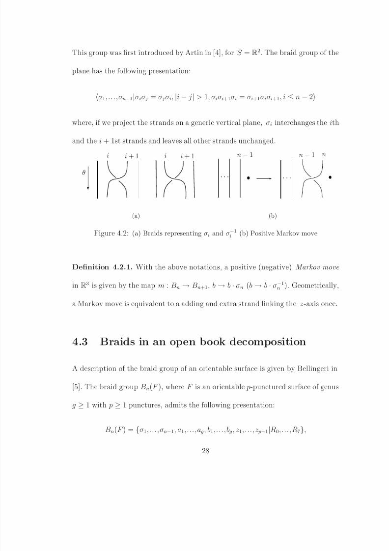
σ1,...,σn−1|σiσ j = σ j σi, |i − j| > 1, σiσi+1σi = σi+1σiσi+1, i ≤ n − 2
where, if we project the strands on a generic vertical plane, σi interchanges the ith
and the i + 1st strands and leaves all other strands unchanged.
ii i + 1i + 1
θ
(a)
n − 1 n − 1 n
· · ·· · ·
(b)
Figure 4.2: (a) Braids representing σi and σ−1i (b) Positive Markov move
Definition 4.2.1. With the above notations, a positive (negative) Markov move
in R3 is given by the mapm
:Bn → Bn+1
,b → b · σn
(b → b · σ
−1
n). Geometrically,
a Markov move is equivalent to a adding and extra strand linking the z-axis once.
4.3 Braids in an open book decomposition
A description of the braid group of an orientable surface is given by Bellingeri in
[5]. The braid group Bn(F ), where F is an orientable p-punctured surface of genus
g ≥ 1 with p ≥ 1 punctures, admits the following presentation:
Bn(F ) = σ1,...,σn−1, a1,...,ag, b1,...,bg, z1,...,z p−1|R0,...,R7,
28
8/3/2019 Elena Pavelescu- Braids and Open Book Decompositions
http://slidepdf.com/reader/full/elena-pavelescu-braids-and-open-book-decompositions 36/66
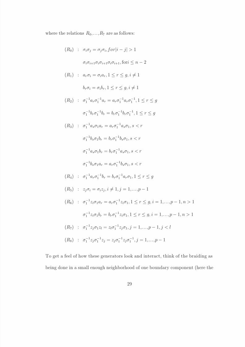
where the relations R0,...,R7 are as follows:
(R0) : σiσ j = σ jσi,for|i − j| > 1
σiσi+1σiσi+1σiσi+1, fori ≤ n − 2
(R1) : arσi = σiar, 1 ≤ r ≤ g, i = 1
brσi = σibr, 1 ≤ r ≤ g, i = 1
(R2) : σ−11 arσ−1
1 ar = arσ−11 arσ−1
1 , 1 ≤ r ≤ g
σ−11 brσ−1
1 br = brσ−11 brσ−1
1 , 1 ≤ r ≤ g
(R3) : σ−11 asσ1ar = arσ−1
1 asσ1, s < r
σ−11 bsσ1br = brσ−1
1 bsσ1, s < r
σ−11 asσ1br = brσ−1
1 asσ1, s < r
σ−11 bsσ1ar = arσ−1
1 bsσ1, s < r
(R4) : σ−11 arσ−1
1 br = brσ−11 arσ1, 1 ≤ r ≤ g
(R5) : z jσi = σiz j , i = 1, j = 1,...,p − 1
(R6) : σ−11 ziσ1ar = arσ−1
1 ziσ1, 1 ≤ r ≤ g, i = 1,...,p − 1, n > 1
σ−11 ziσ1br = brσ−1
1 ziσ1, 1 ≤ r ≤ g, i = 1,...,p − 1, n > 1
(R7) : σ−11 z jσ1zl = zlσ
−11 z jσ1, j = 1,...,p − 1, j < l
(R8) : σ−11 z jσ−1
1 z j = z jσ−11 z jσ−1
1 , j = 1,...,p − 1
To get a feel of how these generators look and interact, think of the braiding as
being done in a small enough neighborhood of one boundary component (here the
29

8/3/2019 Elena Pavelescu- Braids and Open Book Decompositions
http://slidepdf.com/reader/full/elena-pavelescu-braids-and-open-book-decompositions 37/66
monodromy map is the identity) and of the generators zi, ai and bi as being elements
in π1(page) (see Figure 4.3). These generators should not be though of as lying on
a specific page but intersecting the pages transversely between different values of
θ. A generator given by the topology of the page can be parametrized by c :
[0, 1] → Σ × [θ1, θ2], c(t) = (γ (t), δ(t)), where γ : [0, 1] → Σ and δ : [0, 1] → [θ1, θ2]
is strictly increasing. While the stabilizations given by the Markov moves will
always be assumed to be performed on the nth strand of a n-strand braid, the
loops representing the generators given by the topology of the page will always be
assumed to come out of the first strand of a braid.
z
b
a θ
Figure 4.3: Generators of the braid group of a surface.
In an open book decomposition the Markov moves are defined in the neighbor-
hood of each binding component in the same way as in the standard model. The
action corresponding to the conjugation in the standard model should take into
30

8/3/2019 Elena Pavelescu- Braids and Open Book Decompositions
http://slidepdf.com/reader/full/elena-pavelescu-braids-and-open-book-decompositions 38/66
account the monodromy map. We are going to fix the monodromy page, call it Σ0,
and we are going to read all the braid words starting at this page and moving in
the increasing θ direction.
First, there is an action given by b → σ · b · σ−1, where σ is a word in the braid
generators σi’s. This is not influenced by the monodromy map, as φ is identity near
the ∂ Σ. We are going to refer to this as to a b-conjugation .
Second, there is an action given by b → c · b · φ−1(c−1), where c is any of the ai,
bi, zi or their inverses. We are going to refer to this as to a t-conjugation . Note that
by applying the monodromy map to the loop representing φ−1(c−1) when passing
through Σ0 we get a loop representing c−1.
4.4 Algebraic interpretation of the Markov theo-
rem in an open book decomposition
In this section we make the connection between the braid isotopies mentioned in
section 4.1 and the elements of the braid group introduced in the previous section.
Theorem 4.4.1. Let M be a 3-dimensional, closed, oriented manifold and (L, π)
an open book decomposition for M . Let B0 and B1 be closures of two elements of the
braid group. Then B0 and B1 are isotopic as braids in M if and only if they differ
by b- and t-conjugations in the braid group. They represent the same topological
31

8/3/2019 Elena Pavelescu- Braids and Open Book Decompositions
http://slidepdf.com/reader/full/elena-pavelescu-braids-and-open-book-decompositions 39/66
knot type if and only if they differ by b- and t-conjugations and stabilizations in the
braid group.
Proof. Away from the binding the contact planes and the planes tangent to the
surface almost coincide, thus a braid isotopy is equivalent to a transverse isotopy.
We are going to have a look at the two different types of actions.
For a b-conjugation : If we see the braid generators in a small enough neigh-
borhood of the binding, such a conjugation will preserve the braid isotopy class.
The arcs involved in the conjugation may be assumed close enough to the circle
r = , z = 0, which is in braid form for > 0. When projected on the cylinder of
radius R, where R is large enough that all points p on the strands involved in the
conjugation are such that r( p) < R, the braid conjugation represents a sequence of
type II Reidemeister moves.
For a t-conjugation : In this case, the conjugation is a sequence of conjugations
with the a, b and z generators or their inverses. Let ( p,θ1) ∈ Σθ1 be the starting
point of a loop lc representing the element c and ( p,θ2) ∈ Σ2 be its ending point.
Let ( p,θ2) ∈ Σθ2 be the starting point of a loop lφ−1(c−1) representing φ−1(c−1)
and ( p,θ3) ∈ Σθ3 be its ending point. We want to isotop lc · lφ−1(c−1) to the curve
p × [θ1, θ3]. The cutting page Σ0 interposes itself between lc and lφ−1(c−1). As we
move lφ−1(c−1) through Σ0 and apply the monodromy map φ to it we get a new curve
lc−1 representing c−1. We want to isotop lc · lc−1 to the curve p × [θ1, θ3]. This is
certainly possible, as the the arc lc · lc−1 is disjoint form Σ0 and can be isotoped in
32

8/3/2019 Elena Pavelescu- Braids and Open Book Decompositions
http://slidepdf.com/reader/full/elena-pavelescu-braids-and-open-book-decompositions 40/66
Σ × [θ1, θ3] around the topology of the page to p × [θ1, θ3]. This isotopy can be
realized so that the θ coordinate is left unchanged and thus it is an isotopy through
braids.
We now look at the converse. We assume that two braids are isotopic in the
complement of the binding and want to see that they are related by b- and t-
conjugations. Fix again the cutting page Σ0 and consider a braid β which may be
assumed to intersect Σ0 in a small neighborhood of L1. We want to arrange that
the isotopy fixes the endpoints of β on the cutting page. If this is the case, the
isotopy can be seen in Σ × [0, 1] and the and the problem is reduced to the product
case discussed in Section 4.3 and thus are represented by the same word in the braid
group.
If the endpoints of β on the cutting page are not fixed, we can modify the
isotopy in such a way that they remain fixed. Given an isotopy β t from β 0 = β
to β 1 we construct a new isotopy β t where β 0 = β 0 and β 1 is β 1 after some b-
and t-conjugations and such that the intersection of β t with Σ0 is fixed. Say that
the endpoint of one of the strands of β , describes a curve γ ⊂ Σ0 troughout the
isotopy. First, modify the isotopy such that right at the endpoint of γ , the strand
strand looks like p × [0, ]. Then, slide p × 2
along Σ × 2
back in a small
neighborhood of L1 such that p × [0, ] is replaced by γ 1 · γ −1
1⊂ Σ × [0, ]. Now, by
shifting the whole isotopy by in the negative θ direction we find that the endpoint
of the given strand on Σ0 is left unchanged by the new isotopy. The isotopy β t is
33
8/3/2019 Elena Pavelescu- Braids and Open Book Decompositions
http://slidepdf.com/reader/full/elena-pavelescu-braids-and-open-book-decompositions 41/66
left unchanged on the other strands. We repeat the process for all other strands.
Notice that we can do this without having the corresponding γ strands interfere
one with the other, by nesting them with respect to the θ direction.
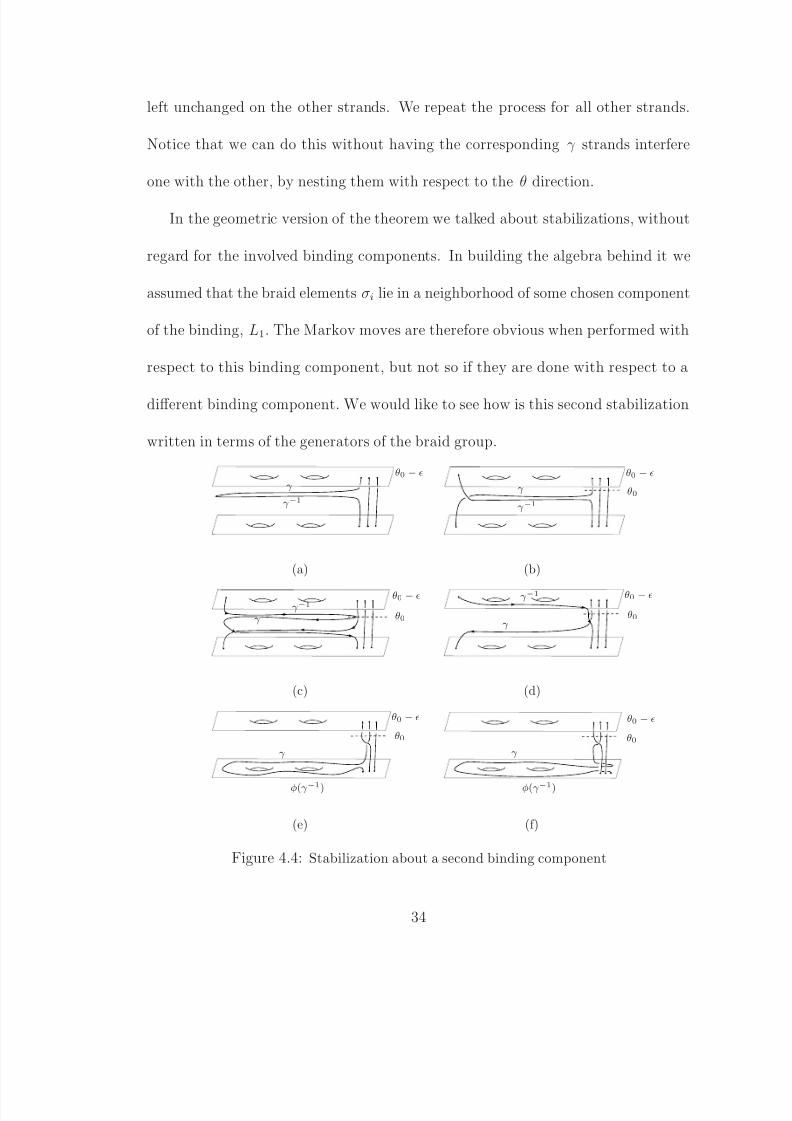
In the geometric version of the theorem we talked about stabilizations, without
regard for the involved binding components. In building the algebra behind it we
assumed that the braid elements σi lie in a neighborhood of some chosen component
of the binding, L1. The Markov moves are therefore obvious when performed with
respect to this binding component, but not so if they are done with respect to a
different binding component. We would like to see how is this second stabilization
written in terms of the generators of the braid group.
γ
γ −1
θ0 −
(a)
γ
γ −1θ0
θ0 −
(b)
γ γ −1
θ0
θ0 −
(c)
γ
γ −1
θ0
θ0 −
(d)
φ(γ −1)
γ
θ0
θ0 −
(e)
φ(γ −1)
γ
θ0
θ0 −
(f)
Figure 4.4: Stabilization about a second binding component
34
8/3/2019 Elena Pavelescu- Braids and Open Book Decompositions
http://slidepdf.com/reader/full/elena-pavelescu-braids-and-open-book-decompositions 42/66
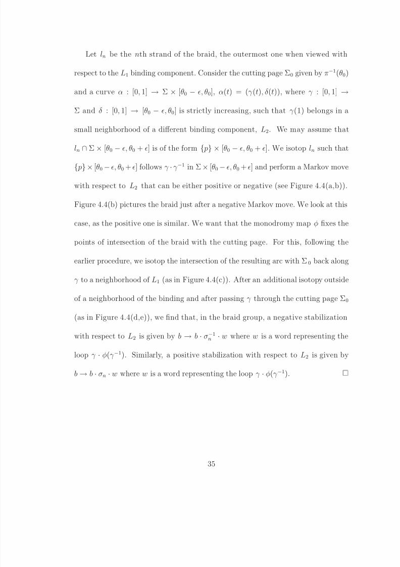
Let ln be the nth strand of the braid, the outermost one when viewed with
respect to the L1 binding component. Consider the cutting page Σ0 given by π−1(θ0)
and a curve α : [0, 1] → Σ × [θ0 − , θ0], α(t) = (γ (t), δ(t)), where γ : [0, 1] →
Σ and δ : [0, 1] → [θ0 − , θ0] is strictly increasing, such that γ (1) belongs in a
small neighborhood of a different binding component, L2. We may assume that
ln ∩ Σ × [θ0 − , θ0 + ] is of the form p × [θ0 − , θ0 + ]. We isotop ln such that
p × [θ0 − , θ0 + ] follows γ · γ −1 in Σ × [θ0 − , θ0 + ] and perform a Markov move
with respect to L2 that can be either positive or negative (see Figure 4.4(a,b)).
Figure 4.4(b) pictures the braid just after a negative Markov move. We look at this
case, as the positive one is similar. We want that the monodromy map φ fixes the
points of intersection of the braid with the cutting page. For this, following the
earlier procedure, we isotop the intersection of the resulting arc with Σ0 back along
γ to a neighborhood of L1 (as in Figure 4.4(c)). After an additional isotopy outside
of a neighborhood of the binding and after passing γ through the cutting page Σ0
(as in Figure 4.4(d,e)), we find that, in the braid group, a negative stabilization
with respect to L2 is given by b → b · σ−1n · w where w is a word representing the
loop γ · φ(γ −1). Similarly, a positive stabilization with respect to L2 is given by
b → b · σn · w where w is a word representing the loop γ · φ(γ −1).
35
8/3/2019 Elena Pavelescu- Braids and Open Book Decompositions
http://slidepdf.com/reader/full/elena-pavelescu-braids-and-open-book-decompositions 43/66
Chapter 5
On the transversal simplicity of
the unknot
In [10], Birman and Wrinkle proved that exchange reducibility implies transver-
sal simplicity. As a consequence, Birman and Menasco’s paper [8] shows that the
m-component unlink is transversely simple. While exchange reducibility does not
seem to work in more general settings, the unknot remains transversely simple in
a tight contact structure. Eliashberg proved this fact in [11]. Later, Etnyre proved
in [14] that positive torus knots are transversely simple. In this chapter we reprove
Eliashberg’s original theorem using braid theoretical techniques.
36

8/3/2019 Elena Pavelescu- Braids and Open Book Decompositions
http://slidepdf.com/reader/full/elena-pavelescu-braids-and-open-book-decompositions 44/66
5.1 Braid foliations
Definition 5.1.1. Let (M, ξ) be a 3-dimensional contact manifold. A topological
class of knots T is called transversely simple if any two transverse representatives
of T having the same self-linking number are transversely isotopic.
Further, we are looking at how an embedded surface in M may sit with respect
to an open book decomposition (Σ, φ) for M . This ideas were first introduced and
studied by Birman and Menasco. Let U ⊂ M be an embedded unknot together with
an embedded disk D such that ∂D = U . By Theorem 3.2.1, U may be assumed to
be braided about the binding of (Σ, φ). The intersection of D with the pages of the
open book induce a foliation on D, the braid foliation .
We may assume that D is in general position in the following sense:
i) D intersects the binding L transversely, finitely many times in such a way that
up to orientation the binding and the normal direction to the disk coincide
ii) In a neighborhood of such an intersection point D is radially foliated (as in
Figure 5.5(a))
iii) All but finitely many pages Σθ meet D transversely and those which do not
are tangent to Σθ at points which are either saddle points or local extremes
with respect to the parameter θ.
iv) The tangency points described in iii) are all on different pages
37

8/3/2019 Elena Pavelescu- Braids and Open Book Decompositions
http://slidepdf.com/reader/full/elena-pavelescu-braids-and-open-book-decompositions 45/66
v) U has a neighborhood N (U ) in M such that N (U ) ∩ D is foliated by arcs
transverse to U . Also, the oriented foliation lines go from inside D transversely
towards U in this neighborhood.
We would like to isotop D such that there are no singularities given by local extremes
with respect to the parameter θ. This requires few more definitions and results.
Definition 5.1.2. Let F be an oriented singular foliation on Σ. Let Γ ⊂ Σ be a
properly embedded 1-manifold. We say that Γ divides F if
1) Γ F
2) Σ \ Γ = Σ+ Σ−, Σ± = ∅
3) ∃ a vector field −→w on Σ and a volume form ω on Σ such that
i) −→w directs F
ii) −→w is expanding ω on Σ+ and contracting ω on Σ−
iii) −→w points out of Σ+(and into Σ−).
Definition 5.1.3. A vector field −→v on a contact manifold (M, ξ) is called a contact
vector field −→v if its flow preserves ξ.
Definition 5.1.4. A surface Σ ⊂ (M, ξ) is said to be convex if there exists a contact
vector field −→v transverse to Σ.
Theorem 5.1.5. For a convex surface Σ as above there exists a dividing set Γ given
by the points on Σ where −→v ∈ ξ.
38
8/3/2019 Elena Pavelescu- Braids and Open Book Decompositions
http://slidepdf.com/reader/full/elena-pavelescu-braids-and-open-book-decompositions 46/66
Lemma 5.1.6. (Legendrian Realization Principle) Let γ be an embedded 1-manifold
on a convex surface Σ such that each component of Σ \ γ intersects a dividing set
Γ. Then Σ can be isotoped through convex surfaces such that γ is Legendrian.
Lemma 5.1.7. Let (Σ, φ) be an open book decomposition for M and ξ a supported
tight contact structure. Let S ⊂ M be an embedded surface. Then S can be isotoped
in such a way that its braid foliation has no tangency points given by local extremes
with respect to the parameter θ.
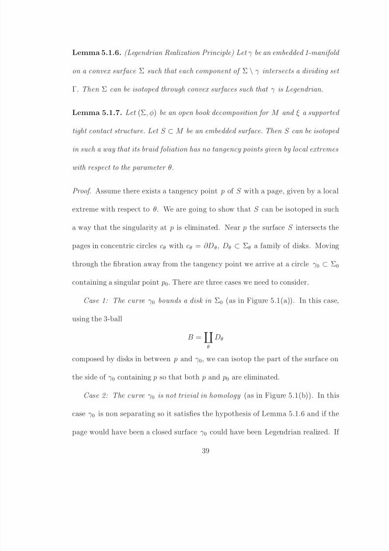
Proof. Assume there exists a tangency point p of S with a page, given by a local
extreme with respect to θ. We are going to show that S can be isotoped in such
a way that the singularity at p is eliminated. Near p the surface S intersects the
pages in concentric circles cθ with cθ = ∂Dθ, Dθ ⊂ Σθ a family of disks. Moving
through the fibration away from the tangency point we arrive at a circle γ 0 ⊂ Σ0
containing a singular point p0. There are three cases we need to consider.
Case 1: The curve γ 0 bounds a disk in Σ0 (as in Figure 5.1(a)). In this case,
using the 3-ball
B =
θ
Dθ
composed by disks in between p and γ 0, we can isotop the part of the surface on
the side of γ 0 containing p so that both p and p0 are eliminated.
Case 2: The curve γ 0 is not trivial in homology (as in Figure 5.1(b)). In this
case γ 0 is non separating so it satisfies the hypothesis of Lemma 5.1.6 and if the
page would have been a closed surface γ 0 could have been Legendrian realized. If
39
8/3/2019 Elena Pavelescu- Braids and Open Book Decompositions
http://slidepdf.com/reader/full/elena-pavelescu-braids-and-open-book-decompositions 47/66
so, the disk bounded by the Legendrain curve γ 0 on S would be an overtwisted
disk, contradicting the hypothesis. We can still apply Lemma 5.1.6, by taking
Σ = Σ0 ∪idL Σ 1
2
and looking at γ 0 ⊂ Σ. The surface Σ is closed, with dividing
curve Γ = L.
γ0
(a)
γ0
(b)
γ0
δδ1 δ2
(c)
Figure 5.1: (a) Homotopically trivial γ (b) Homologically trivial γ not bounding a disk
(c) Homologically essential γ
Case 3: The curve γ 0 is trivial in homology but does not bound a disk in Σ0 (as
in Figure 5.1(c)). Consider Σ as defined above. The curve γ 0 ⊂ Σ may not satisfy
the hypothesis of Lemma 5.1.6, as there might be a component of Σ \ γ 0 which
does not intersect the dividing set, Γ. If so, then consider a non-separating curve δ
in this component. The curve δ can be Legendrian realized. This can be done by
looking at an annulus neighborhood of δ. This annulus has a neighborhood contac-
tomorphic to a neighborhood N of the annulus in the xy-plane in (R3, ξstd)/x∼x+1.
The neighborhood N can be replaced with a new neighborhood which introduces
two new singularity lines and two new components to the dividing set. The new
surface has a dividing set Γ = Γ ∪ δ1, δ2, where δ1 and δ2 are curves parallel to δ,
in a small neighborhood of δ (as in Figure 5.1(c)). With respect to Γ, γ 0 satisfies
the hypothesis of Lemma 5.1.6 and therefore can be Legendrian realized. This trick
40

8/3/2019 Elena Pavelescu- Braids and Open Book Decompositions
http://slidepdf.com/reader/full/elena-pavelescu-braids-and-open-book-decompositions 48/66
was used by Honda in [16] and is called super Legendrian realization. As in Case 2
this gives rise to an overtwisted disk.
In Chapter 2 we have introduced the notion of a characteristic foliation for an
embedded surface S ⊂ M . This foliation and the braid foliation described above
have the same distribution of singularities along S . In a neighborhood of the binding
L the contact structure looks like the standard one, dz+r2dθ and by perturbing S we
can make the normal to S and the binding align at the intersection points, having a
small disk around the intersection point radially foliated, as in Figure 5.5(a). Away
from the binding the contact planes almost coincide with the planes tangent to
the pages and thus, modulo a small perturbation the two foliations also coincide
here. The two foliations are topologically conjugate by a homeomorphism closed
to the identity. This means that from the perspective of the pictures they are the
same. Consider D a spanning disk for an unknot in M . It follows from the general
L
N
D
(a)
L
N
D
(b)
page
N N
D
(c)
page
N
N
D
(d)
Figure 5.2: (a,b)Positive and negative elliptic singularities (c,d) Positive and negative
hyperbolic singularities
position requirements and Lemma 5.1.7 that D can be isotoped in such a way that
the singularities of its braid foliation are either elliptic, given by the intersections
41

8/3/2019 Elena Pavelescu- Braids and Open Book Decompositions
http://slidepdf.com/reader/full/elena-pavelescu-braids-and-open-book-decompositions 49/66
with the binding (as in Figure 5.2(a,b)), or hyperbolic, given by saddle points of D
(as in Figure 5.2(c,d)).
Further, condition iv) satisfied by a disk in general position, implies that there
are no foliation lines connecting two hyperbolic singularities in the braid foliation of
D. A generic braid foliation for D looks like the one in Figure 5.3. In this picture,
the elliptic singularities are denoted by filled dots while the hyperbolic singularities
are denoted by empty dots.
Figure 5.3: Induced braid foliation on D.
A sign can be assigned to each elliptic or hyperbolic singularity in the following
way. An elliptic singularity is positive (negative) if the binding intersects the disk
D in the direction consistent with (opposite to) N , the normal direction to D (as
in Figure 5.2(a,b)). Define e+ (e−) to be the number of positive (negative) elliptic
singularities.
A hyperbolic singularity is positive (negative) if the normal N to D at the
42
8/3/2019 Elena Pavelescu- Braids and Open Book Decompositions
http://slidepdf.com/reader/full/elena-pavelescu-braids-and-open-book-decompositions 50/66
intersection point, is consistent with (opposite to) the normal direction to the page
at that point, N (as in Figure 5.2(c,d)). Define h+ (h−) to be the number of
positive (negative) hyperbolic singularities.
Definition 5.1.8. Let e be an elliptic singularity in the braid foliation of D, as
above. The valence of e, v(e), is defined as the number of hyperbolic singularities
adjacent to e.
In [6], Bennequin found a way of writing the self-linking number in terms of the
singularities in a foliation.
Lemma 5.1.9. Let U be an unknot spanning the embedded disk D and consider the
braid foliation of D as described above. Then sl(U ) = (e− − h−) − (e+ − h+).
Definition 5.1.10. Associate to a foliation F of D the number
c(F ) = e+
+ e− + h+
+ h−,
that is the number of its singularities, and call c(F ) the complexity of F .
5.2 Transverse stabilizations and braid destabi-
lizations
Lemma 5.2.1. Let e be a negative elliptic singularity in the braid foliation of the
disk D, ∂D = U , and let h be an adjacent negative hyperbolic singularity that is
43
8/3/2019 Elena Pavelescu- Braids and Open Book Decompositions
http://slidepdf.com/reader/full/elena-pavelescu-braids-and-open-book-decompositions 51/66
also adjacent to U . Then U can be transversely isotoped (as in Figure 5.4(a)) so
that both e and h are eliminated.
Proof. The foliation we see on the disk V is the braid foliation. By slightly per-
turbing it we get the characteristic foliation on V . This foliation determines how
the contact structure looks like in a neighborhood of V in M . Using Theorem 2.1.7,
we look for a disk V 0 embedded in (R3, ξstd), with the same characteristic foliation.
Consider the disc V 0 ⊂ (R3, ξstd) traced by the isotopy
(s, t) → (t − 3s2
, st − s3
, 18s), t ∈ [−1, 1], s ∈ [−1.1, 1.1]
The disk V 0 has the same characteristic foliation as V and for each fixed value of t,
the curve s → (t−3s2, st−s3, 18s), s ∈ [−1.1, 1.1] remains transverse to the contact
planes, as the form dz − ydx evaluates to 18 + 6s2(t − s2) > 0 on the tangent vector
−6s, t − 3s2, 18.
Lemma 5.2.2. Let e be an elliptic singularity in the braid foliation of the disk D,
∂D = U , such that v(e) = 1 and let h be its only adjacent hyperbolic singularity. If
h and e are of the same sign then U can be transversely isotoped so that both e and
h are eliminated. We are going to refer to this isotopy as to a braid destabilization.
Proof. As the foliation is oriented in such a way that the flowlines go towards U
from inside D, e can only be a positive singularity. Up to choice of orientation
on the disk D the situation is identical to that of the previous lemma, except the
t-parameter should be chosen with the opposite orientation.
44

8/3/2019 Elena Pavelescu- Braids and Open Book Decompositions
http://slidepdf.com/reader/full/elena-pavelescu-braids-and-open-book-decompositions 52/66
Definition 5.2.3. A knot K is said to be obtained through a transverse stabilization
of a transverse knot K
if K = δ ∪ β and K
= δ ∪ β
and β ∪ β
bounds a disk with
one positive elliptic and one negative hyperbolic singularity (as in Figure 5.5(b)).
Here the term transverse refers to the position with respect to the characteristic
foliation.
_
_+ +
U
(a)
+ +
U
(b)
Figure 5.4: Part of D before and after the elimination of a negative hyperbolic singularity
adjacent to U .
Note that through a transverse stabilization the self-linking number is decreased
by 2. The following is a well known lemma, but it’s only sketched in the present
literature. We give a more detailed proof.
Lemma 5.2.4. If K 1 and K 2 are obtained through a transverse stabilization from
two transversely isotopic knots K 1 and K 2, then K 1 and K 2 are themselves trans-
versely isotopic.
45

8/3/2019 Elena Pavelescu- Braids and Open Book Decompositions
http://slidepdf.com/reader/full/elena-pavelescu-braids-and-open-book-decompositions 53/66
Proof. Since K 1 and K 2 are transversely isotopic we may assume K 1 = K 2 = K .
Let D1 and D2 be the disks given by the two stabilizations (as the shaded disk in
Figure 5.5(c)). Let e1, h1 and e2, h2 be the pairs of singularities on D1 and D2 and
α1, α2 the two Legendrian arcs formed by the stable manifolds of h1 and h2. We
may transversely isotop K so that K 1 \ K lies arbitrarily close to α1 and similarly
for K 2 and α2. We can see this in Figure 5.5(c). The pictured part of the knot can
be brought towards the α-arc, as indicated by arrows as in Figure 5.5(b), remaining
transverse to the characterstic foliation. The claim in the lemma follows from the
following three additional lemmas.
+
(a)
+
(b)
+
α
h
(c)
Figure 5.5: (a) Disk foliation of complexity 1 (b) Valence 1 elements in E U (c) Stabiliza-
tion disk
Lemma 5.2.5. There exists a contact isotopy preserving K taking the endpoint of
α1 in D1 to the endpoint of α2 in D2.
Lemma 5.2.6. There exists a contact isotopy preserving K taking α1 to α2.
Proof. Consider p1 the common starting point of α1 and α2 together with a neigh-
borhood N ( p1) contactomorphic to a neighborhood of the origin in (R3, ξstd), N (0).
46
8/3/2019 Elena Pavelescu- Braids and Open Book Decompositions
http://slidepdf.com/reader/full/elena-pavelescu-braids-and-open-book-decompositions 54/66
Consider ξstd given by the 1-form dz + r2dθ. We identify α1 ∩ N ( p1) with the arc
N (0) ∩ (θ = θ1) ∩ (z = 0) and α2 ∩ N ( p1) with the arc N (0) ∩ (θ = θ2) ∩ (z = 0),
for θ1 = θ2. There is an isotopy given by ψt(r,θ,z) = (r, (1 − t)θ1 + tθ2, z), t ∈ [0, 1],
that takes N (0) ∩ (θ = θ1) ∩ (z = 0) to N (0) ∩ (θ = θ2) ∩ (z = 0). Pulling this back
through the contactomorphism gives an isotopy between α1 ∩ N ( p1) and α2 ∩ N ( p1).
A compactness argument completes the proof.
Lemma 5.2.7. Any two stabilizations of K along a fixed Legendrian arc are
transversally isotopic.
Proof. Consider D1 and D2 the two stabilization disks that coincide along the Leg-
endrian arc α. By a small deformation we can assume they coincide in a small
neighborhood of the α arc. As described above, the knot of can be transversely
isotoped to such a neighborhood.
5.3 In a tight contact structure the unknot is
transversely simple
Theorem 5.3.1. Let (M, ξ) be a 3-dimensional contact manifold supported by the
open book decomposition (L, π). If (M, ξ) is tight then the unknot is transversely
simple.
Proof. Considering an arbitrary representative of the unknot, U ⊂ M , and D ⊂ M
47
8/3/2019 Elena Pavelescu- Braids and Open Book Decompositions
http://slidepdf.com/reader/full/elena-pavelescu-braids-and-open-book-decompositions 55/66
an embedded disk with ∂D = U . Using Lemma 5.2.1, the braid foliation on D may
be assumed to have no couples consisting of a negative hyperbolic singularity and
a negative elliptic singularity adjacent to U .
First, we show that any transverse representative of the unknot of maximal self-
linking number can be transversally isotoped to the trivial braid, that is a braid
bounding a disk foliated as in Figure 5.5(a). This proves the theorem in the maximal
self-linking number case. Second, we prove the theorem for arbitrary self-linking
number.
Assume now that U is a transverse representative of the unknot of maximal
self-linking number. The goal is to show that the foliation can be changed into one
of minimal complexity, i.e. such that c(F ) = 1. We are going to see that due to
the maximality of sl(U ), the foliation on D has no negative hyperbolic singularity
with both unstable manifolds going towards U . Having already eliminated the
negative hyperbolic singularities adjacent to U (as in Lemma 5.2.1), all singular
points adjacent to U have positive sign.
Denote by E U the set of elliptic singularities adjacent to U . The elements of
E U are connected in between them through stable manifolds of positive elliptic
singularities. For e ∈ E U define v+(e) to be the number of such connections. If for
all e ∈ E U , v+(e) ≥ 2, then the graph with vertices the elements of E U and edges
the above connections exhibits a cycle. This cycle is the boundary of an overtwisted
disk. As ξ is tight, there must exist an element e ∈ E U with v+(e) ∈ 0, 1.
48
8/3/2019 Elena Pavelescu- Braids and Open Book Decompositions
http://slidepdf.com/reader/full/elena-pavelescu-braids-and-open-book-decompositions 56/66
If E U contains e with v+(e) = 0, then the disk D is foliated as in Figure 5.5(a)
(as it has only one connected component) and therefore c(F ) = 1.
If E U contains e with v+(e) = 1, then a neighborhood of e is foliated like in
Figure 5.5(b). In this case the complexity of the foliation can be reduced by 2
through a braid destabilization as in Lemma 5.2.2.
L1L1L1
L1L1L1L1
L2L2L2
L2L2L2L2
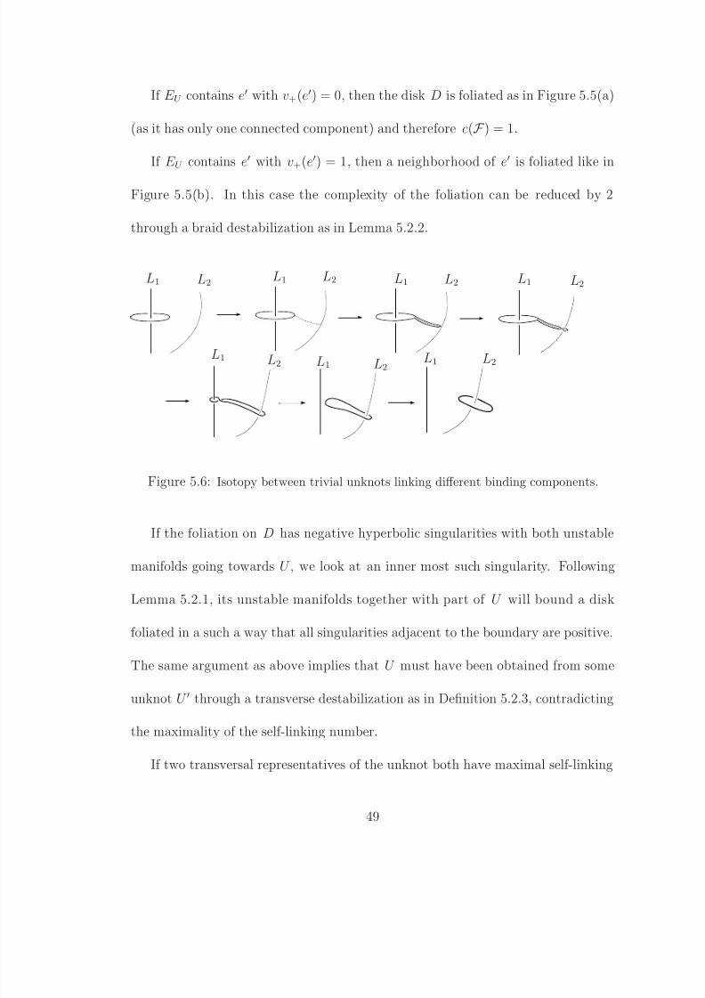
Figure 5.6: Isotopy between trivial unknots linking different binding components.
If the foliation on D has negative hyperbolic singularities with both unstable
manifolds going towards U , we look at an inner most such singularity. Following
Lemma 5.2.1, its unstable manifolds together with part of U will bound a disk
foliated in a such a way that all singularities adjacent to the boundary are positive.
The same argument as above implies that U must have been obtained from some
unknot U
through a transverse destabilization as in Definition 5.2.3, contradicting
the maximality of the self-linking number.
If two transversal representatives of the unknot both have maximal self-linking
49

8/3/2019 Elena Pavelescu- Braids and Open Book Decompositions
http://slidepdf.com/reader/full/elena-pavelescu-braids-and-open-book-decompositions 57/66
number, they are transversely isotopic, as by the above process can be both braid
destabilized by transverse isotopies to a trivial representative, with induced braid
foliation as the on in Figure 5.5(a). If the two trivial unknots are linking the same
binding component then one can isotop one to the other by first shrinking both
in a small enough neighborhood of the respective component, that looks like the a
neighborhood of the z-axis in (R3, ξstd)/z∼z+1. But what if through the destabiliza-
tion process the two unknots end up linking two different binding components, L1
and L2? In this case one of the unknots can be first dragged towards the opposite
binding component, linked through a braid stabilization (the reversed process de-
scribed by Lemma 5.2.2) with this and then freed from linking the initial binding
component through a braid destabilization. This isotopy is described in Figure 5.6.
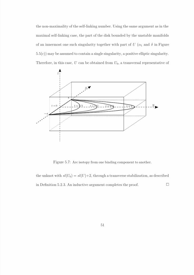
To guarantee that the unknot remains transverse throughout the process the part
of the unknot used to link L1 is dragged towards L2 so that it remains in a small
neighborhood of an arc between U ∩ Σ0 and L2 in a chosen page Σ0. Using the
(x,y,z) coordinates for this neighborhood (where (x, y) are coordinates on the page
and z is the coordinate normal to the page) the actual isotopy can be described by:
f t(x,y,z) = (x, t(1 − ( x )2), z), for t ∈ [0, 1] (see Figure 5.7)
Assume now that U is a transverse unknot which does not have maximal self linking.
In the braid foliation of D there must exist negative hyperbolic singularities having
both unstable manifolds going towards U . Otherwise, as above, after a transverse
isotopy, D can be assumed to be foliated as in Figure 5.5(a), thus contradicting
50
8/3/2019 Elena Pavelescu- Braids and Open Book Decompositions
http://slidepdf.com/reader/full/elena-pavelescu-braids-and-open-book-decompositions 58/66
the non-maximality of the self-linking number. Using the same argument as in the
maximal self-linking case, the part of the disk bounded by the unstable manifolds
of an innermost one such singularity together with part of U (α1 and δ in Figure
5.5(c)) may be assumed to contain a single singularity, a positive elliptic singularity.
Therefore, in this case, U can be obtained from U 0, a transversal representative of
x
y
z
−
t = 1/4 t = 1/2 t = 3/4 t = 1t = 0
Figure 5.7: Arc isotopy from one binding component to another.
the unknot with sl(U 0) = sl(U )+2, through a transverse stabilization, as described
in Definition 5.2.3. An inductive argument completes the proof.
51

8/3/2019 Elena Pavelescu- Braids and Open Book Decompositions
http://slidepdf.com/reader/full/elena-pavelescu-braids-and-open-book-decompositions 59/66
Chapter 6
Surface changes
In the beginning of Chapter 5 we described a generic braid foliation induced on a disk
D bounding the unknot U . We also described ways of changing this foliation through
certain stabilizations and destabilizations. In this chapter we are concerned with a
different type of changes in a foliation, involving adjacent hyperbolic singularities
of the same sign. Originally studied by Birman and Menasco in [8] for (R3
, ξstd) ,
this change in foliation is a key ingredient in proving that the unknot is exchange
reducible in (R3, ξstd).
6.1 Few preliminaries
Consider an open book decomposition (Σ, φ) for the 3-manifold M , a null-homologous
knot K ⊂ M , and a surface S such that ∂S = K . We are going to look at the
braid foliation on S , induced by the intersection with the pages. Following a general
52

8/3/2019 Elena Pavelescu- Braids and Open Book Decompositions
http://slidepdf.com/reader/full/elena-pavelescu-braids-and-open-book-decompositions 60/66
position argument as the one on Chapter 5 and Lemma 5.1.7, there is a natural
way of decomposing S into tiles, according to the singularities of this foliation. This
decomposition was studied by Birman and Menasco in the standard case. The tiles
we are considering are either neighborhoods of a hyperbolic singularity (as in Figure
6.1(a − c)) or foliated disks as in Figure 6.1(d, e). To each tile of type (a), (b) or
(a)
K
(b)
K
K
(c) (d)
K
(e)
Figure 6.1: Possible tiles in the decompositions of S .
(c) we will associate a sign, the same as the one of its singularity.
6.2 Changing order of adjacent saddle points
Theorem 6.2.1. With the above notations, assume a decomposition for S contains
tiles T 1 and T 2 of the same sign which are adjacent at an arc going between two
elliptic points. Let h1 and h2 be the two hyperbolic singularities contained in T 1 and
T 2 and θ1, θ2 ∈ S 1 such that h1 ∈ S ∩ Σθ1 and h2 ∈ S ∩ Σθ2 Then there is an isotopy
F taking S to a surface S such that:
i) F (T 1) and F (T 2) are adjacent regions of the same sign in the decomposition
of S
53

8/3/2019 Elena Pavelescu- Braids and Open Book Decompositions
http://slidepdf.com/reader/full/elena-pavelescu-braids-and-open-book-decompositions 61/66
ii) The decomposition of S outside of a small neighborhood of T 1 ∪ T 2 coincides
with that of S outside of a small neighborhood of F (T 1) ∪ F (T 2)
iii) F (h1) ∈ S ∩ Σθ2 and F (h2) ∈ S ∩ Σθ1
Proof. Roughly, this theorem says that given two adjacent hyperbolic singularities,
of the same sign (as in Figure 6.2(a)) their order with respect to the θ coordinate can
be changed (as in Figure 6.2(b)). In Figure 6.2 the pages are viewed as horizontal
planes. We are going to show that the two singularities can be moved past one
another by showing the existence of a family of disks that can be used to isotop the
surface. The proof of the existence of such disks relies on observing that in a small
neighborhood of the two tiles, T 1 and T 2, the picture can always be standardized,
independent of the open book decomposition.
Consider the two hyperbolic points h1 and h2 as in the hypothesis and without
α
a
a
b
b
c
c
d
d
e
ef
(a)
θ
a
a
b
b
c
c
d
d
e
e
f
f
(b)
Figure 6.2: Neighborhood of adjacent saddle points of the same sign before and after the
isotopy.
loss of generality assume they are both positive. As we proceed in the fibration
54
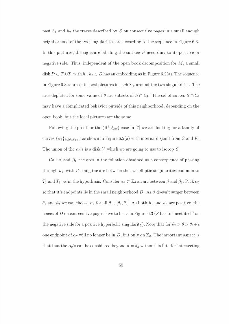
8/3/2019 Elena Pavelescu- Braids and Open Book Decompositions
http://slidepdf.com/reader/full/elena-pavelescu-braids-and-open-book-decompositions 62/66
past h1 and h2 the traces described by S on consecutive pages in a small enough
neighborhood of the two singularities are according to the sequence in Figure 6.3.
In this pictures, the signs are labeling the surface S according to its positive or
negative side. Thus, independent of the open book decomposition for M , a small
disk D ⊂ T 1∪T 2 with h1, h2 ∈ D has an embedding as in Figure 6.2(a). The sequence
in Figure 6.3 represents local pictures in each Σθ around the two singularities. The
arcs depicted for some value of θ are subsets of S ∩ Σθ. The set of curves S ∩ Σθ
may have a complicated behavior outside of this neighborhood, depending on the
open book, but the local pictures are the same.
Following the proof for the (R3, ξstd) case in [7] we are looking for a family of
curves αθθ∈[θ1,θ2+] as shown in Figure 6.2(a) with interior disjoint from S and K .
The union of the αθ’s is a disk V which we are going to use to isotop S .
Call β and β 1 the arcs in the foliation obtained as a consequence of passing
through h1, with β being the arc between the two elliptic singularities common to
T 1 and T 2, as in the hypothesis. Consider αθ ⊂ Σθ an arc between β and β 1. Pick αθ
so that it’s endpoints lie in the small neighborhood D. As β doesn’t surger between
θ1 and θ2 we can choose αθ for all θ ∈ [θ1, θ2]. As both h1 and h2 are positive, the
traces of D on consecutive pages have to be as in Figure 6.3 (S has to meet itself on
the negative side for a positive hyperbolic singularity). Note that for θ2 > θ > θ2 +
one endpoint of αθ will no longer be in D, but only on Σθ. The important aspect is
that that the αθ’s can be considered beyond θ = θ3 without its interior intersecting
55

8/3/2019 Elena Pavelescu- Braids and Open Book Decompositions
http://slidepdf.com/reader/full/elena-pavelescu-braids-and-open-book-decompositions 63/66
D. This means that the αθ arc may be considered for θ ∈ [θ2, θ2 + ].
For the family of arcs αθθ∈[θ1,θ2+], consider the family of disk neighborhoods
V θ parametrized by Lθ : [0, 1] × (−δ, δ) such that αθ = Lθ([0, 1] × 0). Consider
the 3-ball given by the union
V =
V θ, where θ ∈ [θ1, θ2 + ].
Then int(V )
D = ∅. If V has interior disjoint from S and K , we can use V to
+
_
+ _
_
+
θ = θ0 θ = θ1 θ = θint θ = θ2 θ = θ3
α α
β
a a a a a
b b b b bc c c c c
d d d d d
e e e e ef f f f f
Figure 6.3: Traces of a neighborhood of adjacent saddle points of the same sign on
different Σθ’s.
isotop D and change the order of h1 and h2. If there are parts of K or S intersecting
V , we can first isotop these forward in the fibration, outside of V =
V θ, where
θ ∈ [θ1, θ2 + 2
] and then isotop D and change the order of h1 and h2.
56

8/3/2019 Elena Pavelescu- Braids and Open Book Decompositions
http://slidepdf.com/reader/full/elena-pavelescu-braids-and-open-book-decompositions 64/66
Bibliography
[1] B.Aebisher, et all., Symplectic Geometry , Progress in Math., 124, Birkhauser,
Basel, Boston and Berlin, 1994
[2] J.W.Alexander, A lemma on systems of knotted curves, Proc. Nat. Acad. Sci.
USA, 9 (1923), 93-95
[3] J.W. Alexander, Note on Riemann spaces, Bull. Amer. Math. Soc., 26 (1920),
370-372
[4] E.Artin, Theorie der zopfe, Hamburg Abh. 4 (1925), 47-72
[5] P. Bellingeri, On presentations of surface braid groups, Journal of Algebra 274
(2004), 543-563
[6] D.Bennequin, Entrelacements et equations de Pfaff , Asterisque 107-108
(1983), 87-161
[7] J.Birman, E.Finkelstein, Studying surfaces via closed braids, J.of Knot Theory
and its Ramifications, Volume 7, No.3 (1998), 267-334
57

8/3/2019 Elena Pavelescu- Braids and Open Book Decompositions
http://slidepdf.com/reader/full/elena-pavelescu-braids-and-open-book-decompositions 65/66
[8] J.Birman, W.Menasco, Studying Links via Closed Braids V: The Unlink , Trans.
Amer. Math. Soc., 329 (1992), 585-606
[9] J.Birman, W.Menasco, Stabilization in braid groups II: transversal simplicity
of knots , Geometry and Topology, Volume 10 (2006), 1425-1452
[10] J.Birman, N.Wrinkle, On transversally simple knots, J. Differential Geometry,
Volume 55, No. 2 (2000), 325-354
[11] Y.Eliashberg, Legendrian and Transversal Knots in Tight Contact 3-manifolds,
Topological Methods in Modern Mathematics (1991), 171-193
[12] Y.Eliashberg, M.Fraser, Classification of Topologically Trivial Legendrian
Knots, Geometry, Topology and Dynamics, CRM Proceedings and Lecture
Notes, Volume 15 (1998), 17-51
[13] J.Etnyre, Lectures on open book decompositions and contact structures, Clay
Mathematics Proceedings, Volume 5 (2006), 103-142
[14] J.Etnyre, Transversal torus knots, Geometry and Topology, 3 (1999), 253-268
[15] E.Giroux, Geometrie de contact: de la dimension trois vers les dimensions
supeeures, Proceedings of the International Congress of Mathematicians, Vol.
II, 405-414, Higher Ed. Press, Beijing, (2002)
[16] K.Honda, On the classification of tight contact structures, II , J. Differential
Geom., 55(1) (2000), 83-143
58
8/3/2019 Elena Pavelescu- Braids and Open Book Decompositions
http://slidepdf.com/reader/full/elena-pavelescu-braids-and-open-book-decompositions 66/66
[17] A.A. Markov, ¨ Uber die freie ¨ Aquivalenz der geschlossenen Z¨ opfe, Mat. Sobornik
43 (1936), 73-78
[18] S.Yu.Orevkov, V.V.Shevchishin, Markov theorem for transversal links, preprint
2003, math.GT/0112207
[19] P.Ozsvath, Z.Szabo, Heegaard Floer homologies and contact structures, Duke
Math. J. Volume 129, Number 1 (2005), 39-61
[20] R.Skora, Closed braids in 3-manifolds, Mathematische Zeitschrift, Volume 211,
No.1 (1992), 173-187
[21] P.Sundheim, The Alexander and Markov Theorems via Diagrams for Links in
3-Manifolds, Trans. Amer. Math. Soc., 2 (1993), 591-607
[22] W.P.Thurston, H.Winkelnkemper, On the Existence of Contact Forms, Proc.
Amer. Math. Soc. 52 (1975), 345-347
[23] N. Wrinkle, The Markov theorem for transverse knots, arXiv:math/0202055v1