Elements of Topological M-Theory

(with R. Dijkgraaf, S. Gukov, C. Vafa)

Andrew Neitzke

March 2005

Preface

The topological string on a Calabi-Yau threefold X is (looselyspeaking) an “integrable spine” of the Type II string theory onX × R

3,1. Calabi-Yau spaces are the natural target space becausethey preserve some supersymmetry.

The full Type II theory in 10 dimensions is known to develop an11-dimensional Poincare invariance at strong coupling — leadingto the conjecture that there is an M-theory in 11 dimensions whoselow energy limit is 11-dimensional supergravity.

Could something similar happen for the topological string — couldthe Calabi-Yau space X grow an extra dimension? The naturaltarget spaces in this case would be G2 holonomy manifolds. Butwhat is the appropriate low energy action?

Outline

Stable forms and Hitchin’s functionals

Relation to the topological string

Topological M-theory?

Geometric structures and forms

Hitchin introduced new action functionals for which the criticalpoints are geometric structures on a manifold X — e.g. symplecticstructure, complex structure, G2 holonomy metric.

The construction is based on the idea that geometric structures areoften characterized by the existence of particular differential formson X — e.g. presymplectic form ω, holomorphic volume form Ω,associative 3-form Φ — obeying some integrability conditions —e.g. dω = 0, dΩ = 0, dΦ = d ∗ Φ = 0.

Stable forms

A form ω on an n-dimensional manifold X can give rise to ageometric structure because it defines a reduction of the groupGL(n,R) of coordinate changes (structure group of TX ) to thesubgroup that preserves ω.

In order to get the same structure at every point of X ,independent of small perturbations of ω, want ω to benondegenerate and generic in an appropriate sense. What does thismean for a general p-form?

Stable 2-forms

If p = 2, we know how to define a nondegenerate form: it isω = M ijdxi ∧ dxj with detM 6= 0.

A nondegenerate real 2-form in dimension n = 2m can alwayslocally be written

ω = e1 ∧ f1 + · · · + em ∧ fm,

for some choice of basis e1, . . . , em, f1, . . . , fm for T ∗X , varyingover X (“vielbein”). So ω defines a presymplectic structure:reduces GL(2m,R) → Sp(2m,R) at each point.

If dω = 0, then there exist local coordinates(p1, . . . , pm, q1, . . . , qm) such that

ω = dp1 ∧ dq1 + · · · + dpm ∧ dqm.

Then ω defines a symplectic structure.

Stable forms

Another way of expressing the statement that a 2-form ω isnondegenerate is to say that any small perturbation ω → ω + δω

can be undone by a local GL(n,R) transformation. In this sense ωis stable.

This formulation can be generalized to other p-forms: we sayω ∈ Ωp(X ,R) is stable if it lies in an open orbit of the localGL(n,R) action, i.e. if any small perturbation can be undone by alocal GL(n,R) action.

So e.g. there are no stable 0-forms; any 1-form that is everywherenonvanishing is stable; for 2-forms stability is equivalent tonondegeneracy (when n is even!)

Stable 3-forms

What about p = 3? The dimension of ∧3(Rn) grows like n3, butthe dimension of GL(n,R) grows like n2 ⇒ for large enough n,there cannot be stable 3-forms!

In large enough dimensions, every 3-form is different.

Stable 3-forms in dimension 6

But some exceptional examples exist — e.g. n = 6.

dim∧3(R6) = 20

dimGL(6,R) = 36

So consider a stable real 3-form ρ in dimension 6. The stabilizer ofρ inside GL(6,R) has real dimension 36 − 20 = 16; in fact it iseither SL(3,R) × SL(3,R) or SL(3,C) ∪ SL(3,C).

We’re interested in the case of SL(3,C) ∪ SL(3,C).

Stable 3-forms in dimension 6

If ρ has stabilizer SL(3,C) ∪ SL(3,C) it can be written locally inthe form

ρ =1

2

(

ζ1 ∧ ζ2 ∧ ζ3 + ζ1 ∧ ζ2 ∧ ζ3)

where ζ1 = e1 + ie2, ζ2 = e3 + ie4, ζ3 = e5 + ie6, and the ei are abasis for T ∗X , varying over X . The ζi determine an almostcomplex structure on X . If we are lucky, there exist local complexcoordinates (z1, z2, z3) such that ζi = dzi ; in that case we say thealmost complex structure is integrable, i.e. it is an honest complexstructure.

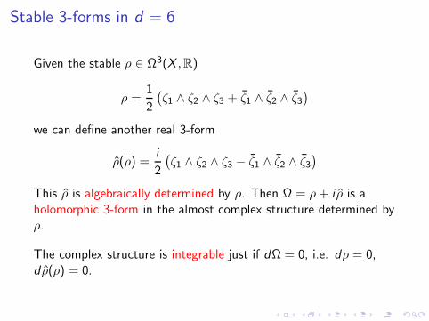
Stable 3-forms in d = 6

Given the stable ρ ∈ Ω3(X ,R)

ρ =1

2

(

ζ1 ∧ ζ2 ∧ ζ3 + ζ1 ∧ ζ2 ∧ ζ3)

we can define another real 3-form

ρ(ρ) =i

2

(

ζ1 ∧ ζ2 ∧ ζ3 − ζ1 ∧ ζ2 ∧ ζ3)

This ρ is algebraically determined by ρ. Then Ω = ρ+ i ρ is aholomorphic 3-form in the almost complex structure determined byρ.

The complex structure is integrable just if dΩ = 0, i.e. dρ = 0,d ρ(ρ) = 0.

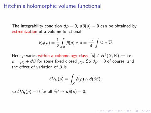
Hitchin’s holomorphic volume functional

The integrability condition dρ = 0, d ρ(ρ) = 0 can be obtained byextremization of a volume functional:

VH(ρ) =1

2

∫

X

ρ(ρ) ∧ ρ =−i

4

∫

Ω ∧ Ω.

Here ρ varies within a cohomology class, [ρ] ∈ H 3(X ,R) — i.e.ρ = ρ0 + dβ for some fixed closed ρ0. So dρ = 0 of course; andthe effect of variation of β is

δVH(ρ) =

∫

X

ρ(ρ) ∧ d(δβ),

so δVH(ρ) = 0 for all δβ ⇒ d ρ(ρ) = 0.

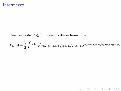
Intermezzo

One can write VH(ρ) more explicitly in terms of ρ:

VH(ρ) =1

2

∫

d6x√

ρa1a2a3ρa4a5a6ρa7a8a9ρa10a11a12εa2a3a4a5a6a7εa8a9a10a11a12a1

Hitchin’s holomorphic volume functional

So extremization of VH , with a fixed [ρ] ∈ H3(X ,R), leads tointegrable complex structures on X , equipped with holomorphic3-forms Ω, such that the real parts of the periods are fixed by[Re Ω] = [ρ]. (Almost “Calabi-Yau structures” on X , except thatwe didn’t say X was Kahler. No Ricci flat metrics here!)

Complex geometry emerges from real 3-forms! A peculiarity ofd = 6.

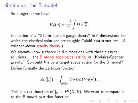
Hitchin vs. the B model

So altogether we have

VH(ρ) =−i

4

∫

Ω ∧ Ω,

the action of a “2-form abelian gauge theory” in 6 dimensions, forwhich the classical solutions are roughly Calabi-Yau structures. (Astripped-down gravity theory.)

We already know a theory in 6 dimensions with these classicalsolutions — the B model topological string, or “Kodaira-Spencergravity.” So could VH be a target space action for the B model?

Define formally the partition function,

ZH([ρ]) =

∫

ρ∈[ρ]Dρ exp (VH(ρ)) .

This is a real function of [ρ] ∈ H3(X ,R). We want to compare itto the B model partition function.

The B model and background dependence

The B model partition function is naively a holomorphic functionof the complex moduli of X , ZB(t). But more precisely, it has abackground dependence: depends on choice of base-pointΩ0 ∈ H3(X ,R), so it should be written ZΩ0

B (t). Here t

parameterizes tangent vectors to the extended Teichmuller space(complex structures together with a choice of holomorphic 3-form):t ∈ H3,0(XΩ0

,C) ⊕ H2,1(XΩ0,C). [Bershadsky-Cecotti-Ooguri-Vafa]

The various ZΩ0B are related by a holomorphic anomaly equation

which gives the parallel transport from one Ω0 to another Ω′0. This

equation has an elegant interpretation. [Witten]

Background dependence as the wavefunction property

Consider H3(X ,R) as a symplectic vector space; then we canquantize it. (Think of R

2 with ω = dp ∧ dq.) The Hilbert spaceconsists of functions ψ which depend on “half the coordinates,”e.g. functions on a Lagrangian subspace (choice of polarization).Different polarizations are related by Fourier-like transforms.

So we can have real polarizations (like ψ(q) orψ(p) =

∫

dq e ipqψ(q)), obtained by splitting H3(X ,Z) into “Aand B cycles” — symplectic marking,H3(X ,Z) = H3(X ,Z)A ⊕ H3(X ,Z)B .

Can also have holomorphic polarizations (like ψ(q + ip) orψ(q + τp)) obtained by splitting H3(X ,C), e.g. Hodge splittingH3(X ,C) =

(

H3,0 ⊕ H2,1)

⊕(

H0,3 ⊕ H1,2)

.

The various ZΩ0B are expressions of the same wavefunction in

different polarizations of H3(X ,R) — polarization given by theHodge splitting determined by Ω0.

Hitchin vs. the B model

So we’ve seen that ZB depends on only half the coordinates ofH3(X ,R) (Lagrangian subspace) and requires a choice ofpolarization. These features are visible already classically (genuszero).

On the other hand, ZH is a function on all of H3(X ,R), anddoesn’t seem to require any choice.

So we can’t say ZH = ZB . Instead, propose that ZH = ZB ⊗ ZB ,or more precisely, ZH is the Wigner function associated to ZB : thisis the phase-space density,

(ZB ⊗ ZB)([ρ]) =

∫

dΦ e−〈Φ,ρB 〉 |ZB(ρA + iΦ)|2.

Here we wrote ZB in the real polarization determined by a choiceof A and B cycles (symplectic marking): ρA = ρ|H3(X ,R)A ,ρB = ρ|H3(X ,R)B .

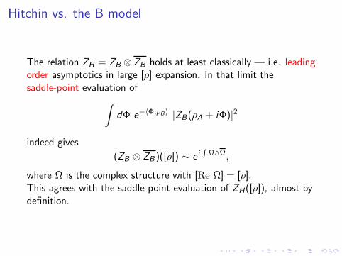
Hitchin vs. the B model

The relation ZH = ZB ⊗ ZB holds at least classically — i.e. leadingorder asymptotics in large [ρ] expansion. In that limit thesaddle-point evaluation of

∫

dΦ e−〈Φ,ρB 〉 |ZB(ρA + iΦ)|2

indeed gives

(ZB ⊗ ZB)([ρ]) ∼ e iR

Ω∧Ω,

where Ω is the complex structure with [Re Ω] = [ρ].This agrees with the saddle-point evaluation of ZH([ρ]), almost bydefinition.

Hitchin vs. the B model

At one-loop the situation is subtler: careful BV quantization showsthat, in order to agree with the known one-loop ZB ⊗ ZB , oneneeds to replace ZH by an extended ZH . [Pestun-Witten]

The extended ZH includes fields describing variations ofgeneralized complex structures. [Hitchin]

Hitchin B model and black holes

The Wigner function of the B model (which we have nowidentified as ZH([ρ])) has appeared recently in another context: itwas conjectured that ZH([ρ]) computes the number of states of ablack hole.

Motivation from the attractor mechanism: suppose we considerType IIB superstring on X × R

3,1. Then we can construct acharged black hole by wrapping a D3-brane on a 3-cycleQ ∈ H3(X ,Z). The complex moduli of X near the horizon thenget fixed to an Ω satisfying [Re Ω] = Q∗.

This is exactly the Ω that Hitchin’s gauge theory constructs if wefix the class [ρ] = Q∗. And ZH([ρ]) is exactly the number of statesof the black hole! [Ooguri-Strominger-Vafa]

So ZH reformulates the B model in a way naturally adapted to thecounting of black hole states.

Hitchin’s symplectic volume functional

What about the A model? This has to do with variations ofsymplectic structures.

Hitchin introduced a functional which produces at its criticalpoints symplectic structures in d = 6.

A stable 4-form σ in d = 6 may be written σ = 12k ∧ k . Then k

gives a presymplectic structure. Define

VS(σ) =1

6

∫

k ∧ k ∧ k =1

3

∫

k ∧ σ.

Varying VS(σ) with [σ] ∈ H4(X ,R) fixed, i.e. σ = σ0 + dγ forsome closed σ0, get

δVS =1

2

∫

k ∧ dδγ,

so δVS = 0 ⇒ dk = 0, i.e. k defines a symplectic structure.

So VS has the same classical solutions as the A model.

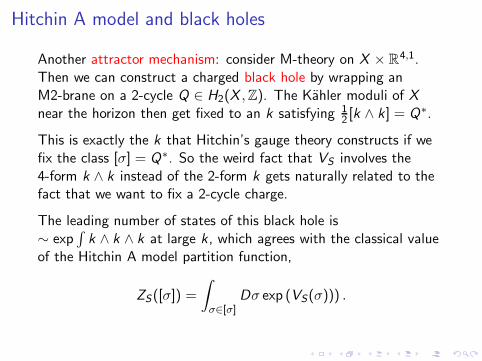
Hitchin A model and black holes

Another attractor mechanism: consider M-theory on X × R4,1.

Then we can construct a charged black hole by wrapping anM2-brane on a 2-cycle Q ∈ H2(X ,Z). The Kahler moduli of X

near the horizon then get fixed to an k satisfying 12 [k ∧ k ] = Q∗.

This is exactly the k that Hitchin’s gauge theory constructs if wefix the class [σ] = Q∗. So the weird fact that VS involves the4-form k ∧ k instead of the 2-form k gets naturally related to thefact that we want to fix a 2-cycle charge.

The leading number of states of this black hole is∼ exp

∫

k ∧ k ∧ k at large k , which agrees with the classical valueof the Hitchin A model partition function,

ZS([σ]) =

∫

σ∈[σ]Dσ exp (VS(σ))) .

Hitchin A model and black holes

It was known before that one can extract counts of BPS states ofwrapped M2-branes in five dimensions from the perturbative Amodel. [Gopakumar-Vafa]

Here we are finding that the Hitchin version of the A model isorganized differently — its partition function seems to be directlycounting the number of states.

Hitchin and topological strings

So Hitchin’s functionals VH and VS in 6 dimensions seem to givereformulations of the target space dynamics of the B model and Amodel topological string theories, naturally adapted to the problemof counting black holes.

We only argued for this classically; it remains to be seen how muchVH and VS can capture about the quantum theories.

These reformulations may be of interest in their own right. Theyare also naturally related to Hitchin’s functional in 7 dimensions.

Stable 3-forms in dimension 7

Another exceptional example — n = 7.

dim∧3(R7) = 35

dimGL(7,R) = 49

So consider a stable real 3-form Φ in dimension 7. The stabilizer ofΦ inside GL(7,R) has dimension 49 − 35 = 14; in one open subsetit is the compact form of G2.

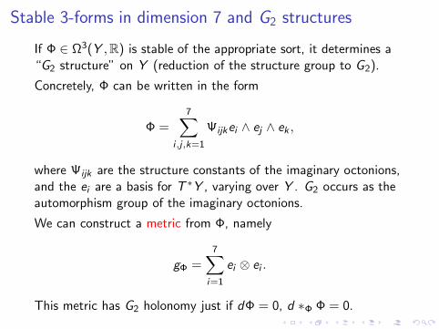
Stable 3-forms in dimension 7 and G2 structures

If Φ ∈ Ω3(Y ,R) is stable of the appropriate sort, it determines a“G2 structure” on Y (reduction of the structure group to G2).

Concretely, Φ can be written in the form

Φ =

7∑

i ,j ,k=1

Ψijkei ∧ ej ∧ ek ,

where Ψijk are the structure constants of the imaginary octonions,and the ei are a basis for T ∗Y , varying over Y . G2 occurs as theautomorphism group of the imaginary octonions.

We can construct a metric from Φ, namely

gΦ =

7∑

i=1

ei ⊗ ei .

This metric has G2 holonomy just if dΦ = 0, d ∗Φ Φ = 0.

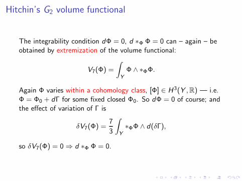
Hitchin’s G2 volume functional

The integrability condition dΦ = 0, d ∗Φ Φ = 0 can – again – beobtained by extremization of the volume functional:

V7(Φ) =

∫

Y

Φ ∧ ∗ΦΦ.

Again Φ varies within a cohomology class, [Φ] ∈ H 3(Y ,R) — i.e.Φ = Φ0 + dΓ for some fixed closed Φ0. So dΦ = 0 of course; andthe effect of variation of Γ is

δV7(Φ) =7

3

∫

Y

∗ΦΦ ∧ d(δΓ),

so δV7(Φ) = 0 ⇒ d ∗Φ Φ = 0.

Hitchin’s G2 volume functional and topological M-theory

So

V7(Φ) =

∫

Y

Φ ∧ ∗ΦΦ

generates G2 holonomy metrics at its critical points. In this senseit is a candidate action for topological M-theory.

By analogy with physical M-theory, one would expect thattopological M-theory on X × S1 should be related to topologicalstring theory on X . Indeed, this V7 can be connected to the A andB models.

Hitchin’s G2 volume functional and topological M-theory

Namely, letting t be the coordinate along S 1 in Y = X × S1, andsplitting

Φ = kdt + ρ

one gets (assuming the constraints k ∧ ρ = 0,2VS (σ) − VH(ρ) = 0)

∗ΦΦ = ρdt + σ

which impliesV7(Φ) = 2VH(ρ) + 3VS(σ)

So topological M-theory seems to reduce to the sum of the A andB models at least in this formal sense.

Hamiltonian reduction

Another perspective on this relation: consider canonicalquantization of topological M-theory on X × R. The phase spaceis then Ω3

exact(X ,R) × Ω4exact(X ,R) (omitting zero modes), with

the symplectic pairing determined by

〈δρ, δσ〉 =

∫

δρ ∧1

dδσ (1)

and the Hamiltonian

H = 2VS(σ) − VH(ρ). (2)

The conditions k ∧ ρ = 0, 2VS(σ) −VH(ρ) = 0 then (should) showup as the diffeomorphism and Hamiltonian constraints, as usual forquantization of a diffeomorphism invariant theory.

The A model and B model appear as conjugate degrees of freedom!

Open questions

There are many open questions:

I How does topological M-theory embed into the physicalstring/M-theory (what quantities does it compute?)

I Can it be used to give a nonperturbative definition of thetopological string? The splitting between A and B models isnot covariant in 7 dimensions — does this mean the A and Bmodels have to be mixed together nonperturbatively? Howshould the 6-dimensional couplings gA, gB be identified?

I What is the meaning of the fact that the A and B modelappear as conjugate variables? (S-duality?) [Nekrasov-Ooguri-Vafa]

I Should the theory be augmented to one which describesgeneralized G2 structures? [Pestun-Witten, Hitchin, Witt]

I Is there a lift to 8 dimensions? [Anguelova-de Medeiros-Sinkovics]