Elements of Matlab and Simulink

Lecture 7

Emanuele Ruffaldi

12th May 2009

Copyright 2009,Emanuele Ruffaldi. This work is licensed under the Creative Commons Attribution-ShareAlike

License.

PARTIAL DIFFERENTIAL EQUATIONS

Introducing PDE

Ordinary Differential Equation

• Derivatives respect a single independent variable

• Solution is a function with arbitrary constants

Partial Differential Equation

• Differential relationship of multiple variables

• Solution is an arbitrary function

• Solution determined by fixing boundary conditions

Notation

Elements of a PDE

Equation Domain

Boundary Conditions

Heat Equation

Heat (or diffusion) equation: models the diffusion of temperature from an initially concentrated distribution

u_t = u_xx

Example of solution is:

u(x,t) = 1/sqrt(t) exp(-x^2/4*t)

Verify using MATLAB Symbolic Toolbox

>> Example lecture7_diffuse

Boundary Problem

The Dirichlet problem is the general problem of finding a function u which solves a PDE for which the values are known on the boundary of a given region

• Given a PDE over RN

• Given a function f that has values over a boundary region of Ω

• Find a function u solving PDE that is differentiable twice in the interior and once on the boundary and assumes the values of f on the boundary

The Neumann problem involves a boundary condition relative to a derivative of the target function

Expressed as u_n

Heat Equation 2D

Heat Equation 2D: diffusion of a quantity along the space and time

u_t = u_xx + u_yy

The general formulation is

u_t = div grad u

Example

Metal block with a rectangular crack. The left side is heated at 100 degrees, the right side heat is flowing to air at constant rate. The others sides are insulated

u = 100 (Dirichlet condition)

u_n = -10 on the right side (Neumann condition)

u_n = 0 on the other boundaries (Neumann condition)

Linear Advection Equation

Linear advection equation: models the constant movement of an initial distribution of u with a speed of –c along x axis. Shape is preserved

u_t = c u_x

For any function q a solution is q(w) where w = x+ct

u(x,t) = q(w) = q(x+ct)

>> Example lecture7_advection

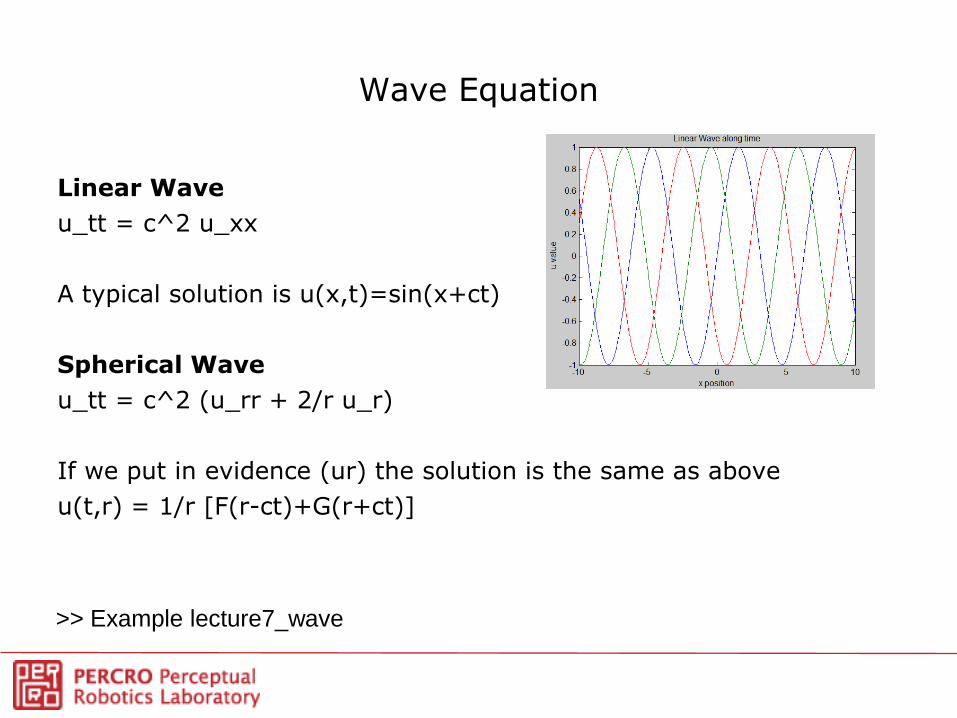
Wave Equation

Linear Wave

u_tt = c^2 u_xx

A typical solution is u(x,t)=sin(x+ct)

Spherical Wave

u_tt = c^2 (u_rr + 2/r u_r)

If we put in evidence (ur) the solution is the same as above

u(t,r) = 1/r [F(r-ct)+G(r+ct)]

>> Example lecture7_wave

Laplace Equation

Laplace Equation

u_xx + u_yy = 0

Poisson Equation

u_xx + u_yy = g(x,y,z)

Helmholt’s Equation

u_xx + u_yy + f(x,y) u = g(x,y,z)

Require boundary conditions for resolution

Basics of FEM

How we can solve PDE numerically when no analytical solution is available?

The Finite Element Method is the most common solution

1. Decompose the Domain in subspaces

2. Approximate the Function with piecewise linear function defined inside each subspace

3. Find the numerical solution for every subspace given the conditions

FDM is the Finite Difference Method is possible but it works better with rectangular domains

FEM 1D

Space discretization

Interpolation Function Linear Combination (Basis)

FEM 2D

Air

Silicon

Generalized approach by decomposing

the domain in unit elements

Families of PDE and use

• Elliptic and Parabolic

• Steady and unsteady heat transfer in solids

• Flows in porous media and diffusion problems

• Electrostatics of dielectric and conductive media

• Potential flow

• Hyperbolic

• Transient and harmonic wave propagation in acoustics and electromagnetics

• Transverse motions of membranes

• Eigenvalue

• Determining natural vibration states in membranes and structural mechanics problems

MATLAB Partial Differential Equation Toolbox

Solves some families of PDE: elliptics, parabolic, hyperbolic and eigenvalue

PDE Toolbox works in the easiest way with 2D Boundary

User Interface (pdetool) and Command line

Steps

1. Define the Domain

2. Define the Boundary function

3. Solve

4. Plot results

Expressing the Geometry

The boundary is expressed by Constructive Solid Geometry

Set composition of fundamental entities

The CSG allows to compose basic entities

1 32 4

-Graphical editing (pdetool)

-initmesh and decsg

-Understand CSG expression

Geometry as Mesh

• The FEM resolution uses a triangular mesh for the spatial discretization of the problem

• The Constructive Geometry produces a closed surface that is later transformed in Mesh

• Refine mesh for improving details on borders or surface features (number of triangles increases)

• Jiggle mesh (quality improves)

Draw Mode

Mesh Mode

Expressing the Boundary Conditions

• Two types of Boundary Conditions

• Dirichlet

• h u=r

• Neumann

• n c grad(u) + qu = g

• e.g. n c grad(u) = 0 means no flux

• Coefficients in bold can be specified with PDE tool

• Export Decomposed geometry and Boundary into Workspace variables

Resolution of PDE

• Solver function depend on the type of problem

• u1=parabolic(u0,tlist,b,p,e,t,c,a,f,d)

• u0 is the initial condition (sized as size(p,2))

• tlist is the time in which let system evolve

• b boundary

• p,e,t geometry

• [c,a,f,d] parameters of

• Automatic Refinement of problem

• [u,p,e,t]=adaptmesh(g,b,c,a,f,options)

• The parabolic equation can be solved keeping time fixed and starting at given condition

• Time Discretization (stages)

• Method of lines

• Allows PDEs in Simulink

Heat Equation 2D

Example

Metal block with a rectangular crack. The left side is heated at 100 degrees, the right side heat is flowing to air at constant rate. The others sides are insulated

u = 100 (left side)

u_n = -10 on the right side

u_n = 0 on the other boundaries

u_t = u_xx + u_yy Create Domain

Set Boundary conditions

Set PDE

Solve

Test

>> Example lecture7_heat2d_pde.m with pdetool

PDE for Simulink

• Simulink Solves ODE equations

• Use Method of Line for making the PDE an ODE problem

• We are interested in using the dynamic resolution of a PDE as part of our simulation

• Update the PDE parameters and inputs along time

• Integration performed by Simulink

• If using Discrete simulation we can let MATLAB do the math

PDE

Problem

Simulink

Block

States

Input

Outputs

One for every node

Time depending

Statitsics (max/min)

Value at node

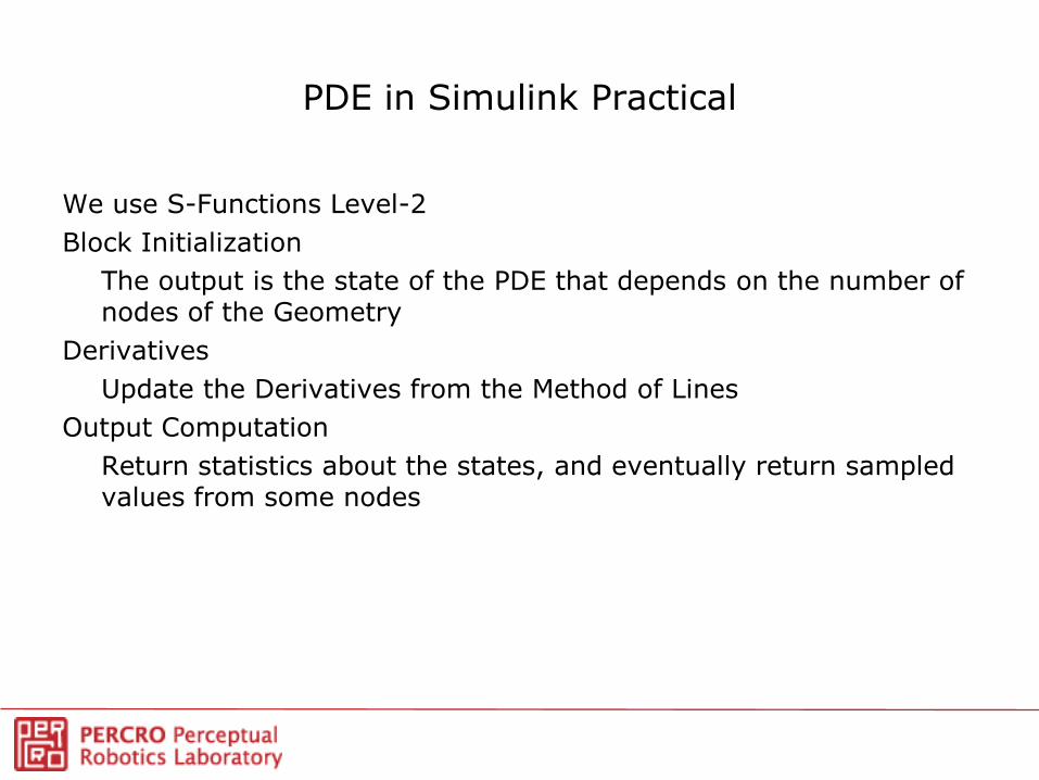
PDE in Simulink Practical

We use S-Functions Level-2

Block Initialization

The output is the state of the PDE that depends on the number of nodes of the Geometry

Derivatives

Update the Derivatives from the Method of Lines

Output Computation

Return statistics about the states, and eventually return sampled values from some nodes

Matrix Form of the FEM

Basic Matrix Formulation

Dirichlet Neumann

Integrated Equation

Thermal Regulation Problem

• If the diffusion is fast there is no

need for space information

• What if we want to use the exact

position of the Thermostat?

PDE is Parabolic

Simulink just needs the Elliptic

Thermal Regulation PDE

• Geometry

• Boundary

• Walls: n grad(T)=0

• Glass: n grad(T)=q (u(1)-T)

• Where u(1) is exterior temperature, T is the internal temperature and q is the thermal conductivity

• Equation

• T' = div( K grad(T) ) + Th u(2)

• u(2) is the heater on or off

• Th is the function of heat flow from the heater based on its position

Thermal Regulation Simulink

The solution for this integration is an S-Function written as M-file

Parameters

• Coordinates of Heater xh,yh and Radius

• Node of the Thermostat

• Initial Temperature T0

• Heater Temperature Th

Input

• State of the Heater

• External Temperature

Output

• State of the Heater

• Maximum Temperature in Room

• Temperature at Thermostat

References

• Books

• An Introduction to Partial Differential Equations with MATLAB,Coleman M., CRC Press, 2005

• Introduction to Partial Differential Equations with MATLAB, Cooper J.M., Birkhause, 1998

• Beginners Guide to Simulation for Physical Engineering: Practical Usage of MATLAB and PDEase, Yutaka Abe, 1999

• Courses

• Introduction to Partial Differential Equations, Doug Moore, 2003

• Introduction to Partial Differential Equations, Showalter, Oregon State University

• MAE502 Partial Differential Equations in Engineering, ASU,2009