Elements in Fruits and Vegetables from Areas of … · Elements in Fruits and Vegetables from Areas...
156
Elements in Fruits and Vegetables from Areas of Commercial Production in the Conterminous United States
Transcript of Elements in Fruits and Vegetables from Areas of … · Elements in Fruits and Vegetables from Areas...

Elements in Fruits and Vegetables from Areas of Commercial Production in the Conterminous United States

Elements in Fruits and Vegetables from Areas of Commercial Production in the Conterminous United States
By HANSFORD T. SHACKLETTE
GEOLOGICAL SURVEY PROFESSIONAL PAPER 1178
A biogeochemical study of selected food plants based on field sampling of plant material and soil
UNITED STATES GOVERNMENT PRINTING OFFICE, WASHINGTON: 1980
UNITED STATES DEPARTMENT OF THE INTERIOR
CECIL D. ANDRUS, Secretary
GEOLOGICAL SURVEY
H. William Menard, Director
Library of Congress Cataloging in Publication DataShacklette, Hansford T.Elements in fruits and vegetables from areas of commercial production in the conterminous
United States.(Geological Survey Professional Paper 1178)Bibliography: p. 28Supt. of Docs, no.: I 19.16:11781. Vegetables—United States—Composition. 2. Fruit—United States—Composition. 3. Vegetables-
United States—Soils—Composition. 4. Fruit—United States—Soils—Composition. 5. Biogeochemistry- United States. 6. Fruit-culture-United States. 7. Truck farming-United States. 8. Soils-United States-Composition. I. Title. II. Series: United States Geological Survey Professional Paper 1178.
SB320.6.S52 641.3's'0973 80-607141
For sale by the Superintendent of Documents, U.S. Government Printing Office Washington, D.C. 20402
CONTENTS
j. II trouuc tion -—••-••—™--™—-—-----——-—---—-™--—™Sampling localities ——————————————
Berrien County, Michigan —————Wayne County, New York ———————Cumberland County, New Jersey Palm Beach County, Florida — Hidalgo County, Texas ———————Imperial County, California ——————Yuma County, Arizona —--—————Twin Falls County, Idaho ———————Yakima County, Washington -----———San Joaquin County, California Mesa County, Colorado ———————
Methods of sampling plants and soils —-— Sampling design ——————————Sampling techniques ————————
Species of plants sampled ————f ru.it s ------—-•—- --—-—-—................Vegetables
Collection and preparation of samplesFruits ——————————— .....x i UILO ......Vegetables ———————— —— —Soils _ — _ - _ • __ — —— • -----
Analytical methods used —————————Plants--— ————— —————— ————— ——
Statistical procedures used in evaluating data
Concentrations of elements in fruits and vegetables Bases for reporting concentrations of elements -----
Page
99
101010111112121213131313171717
Results— ContinuedConcentrations of elements in fruits and vegetables— Continued
Mean concentrations in samples - —— - —— - — - — - —Compositional variation among areas, among fields
within areas, and within fields —— - — — — - ——Analysis of variance -- — — —— - ———— - —— - — —Significant differences in mean element concentra
tions among areas of commercial production ——Concentrations of elements and pH of soils that sup
ported the fruits and vegetables — - —— - — - — -- —Compositional variation among areas and among
fields within areas — — - —— — — -— ——— - — — -Analysis of variance - ——— — - —— — — - — - — -—Significant differences in mean element concen
tration and pH among areas of commercialproduction — -- —— — —— —— — —— -- — — — - ——
Discussion of results — — — ~ — -- —— — — — —— -- — - —— - — - —Trends in element concentrations in fruits and vege-
Among kinds of produce
Among areas of commercial production — - ——— - —Trends in element concentrations in soils supporting
fruits and vegetables — ~ — — - — — —— — — ~ — -— — -Among kinds of produce — — — - — — —— — — — - — —Among areas of commercial production — — —— - ——
Relationships of the element concentrations in fruits andvegetables and the concentrations in soils — - — — — - ——
t-ITVM-MQflr „. _________ __ „„ __________ummary ———— —————— - ———— — — ———— — —Conclusions — — — — — - — — — — — ..———.—— —— .._.... — .. —References cited - — - — ----- -- — — — — — — - —— — —— — -- — —
ILLUSTRATION
Page
19
1919
20
20
2020
2 12 1
2 1
23
242424
2597& t 28 28
Page
FIGURE 1. Map showing locations of counties where fruits and vegetables weresampled ———--—————————————————— —*--—— —-— —-- o
TABLES
TABLE 1. Summary of methods used for analysis of plants and plant ashes and ap proximate lower limits of determination - — -- —— - — - —— — — — — -
2. Summary of methods used for analysis of soils and approximate lower limits oi determination — - — • —— ..... ————— ...... —— ........ —— .... — .... —
3. Components of variance in composition between samples from within a sampling site and between analyses of the same sample -— —— - ——
Page
14
17ill

IV CONTENTS
TABLES 4-20. Elements in ash or dried material, percent ash yield of dried material, Pase and percent dried material yield of fresh fruits and vegetables from areas of commercial production:-I. ^-&iud. &i,ciu gia|JG0 — ~ — — — c AfvrVlpQ' ppD« HjuropGsn gr&p&s -«-— «»-—«— ---««—— --—»--— -»—««•»—«
8. Oranges —— — —— — — -_——__.___ — .--.-—
1 ft Poaro ....... .................... ......... .... . ...__...«..
U Pin me __ ______ _ __ __ _ _ __ __
1 9 /^oKKorrA . ..... ........ . .... . ... ........ ......
13. Carrots ———— - ————————————————————14. Cucumbers ——————————— - ———————————15. Dry beans ———— - ———————— - ——————————
n Pnf nf-rma . ____ ... __ _ . --—-—- ...... __ __ ___ _
lo, &nap Deans ------ ----- — — ——-—«--— .......... «..«._.........
9O TWnatrioQ - — —— - ————— —— —— — — ———— ——
. .. .. .. 34_.... ..... 35—— —— 36
00
„.. .... 40... _ - 42.. .... ... 44. ..... .... 46__ —— 48
4Q.... — 50
CO
.. —— ... 54cc
—— —— 58—— .... 60
21-37. Summary statistics of element concentrations expressed on fresh-, dry-, and ash-weight bases, ash yield of dry material, and dry-material yield of fresh material for each kind of fruit and vegetable col lected in more than one area:21. American grapes ————-——————-—————————————- 6222. Apples ——--———————————————-———————————— 6323. European grapes -——————-———-—————————————— 64*)A dvanofwilt _ _ „ .__ . ..„__ _.........-_......_.-..........-- RK,£ti± t urrcipciruit ---—————————-—-———-—-—-—————-----———---•• uu
Oft J)aaf»VlAa __ ... -MM........................_................_......................... fi7£t\J, i CUCIlCO ——-—————-————————-——-" ——™ -—— U i
28. Plums - ————29. Cabbage ———^Ift P'nrrntc .... .......
31. Cucumbers —— 32. Dry beans —— 33. Lettuce- ————^ A. Pnfr Q t noo ....—.„
35. Snap beans ——
37 Tmrmtnoo ..
ftQ
..... ... —— .... .. —— —— ——— .. —— —— 70717273ri A
7C
in______ _ ___________________ _ _____ ___ 7 7 .... ——— . __ . ..... _ .. „ __ . . __ . 7fi
38-45. Summary statistics of element concentrations expressed on fresh-, dry-, and ash-weight bases, ash yield of dry material, and dry-material yield of fresh material for each kind of fruit and vegetable col lected in only one area:
QB Aanoromio ... _............................................._.....__....„........... 7QOO. /\o£Jclrei££Uo -———•—-—.•—---— — — — -- .......... .....««.. . .......... i jjQQ Oonf almmaa — _ ...... _ ____ ,, ______ _____ ____ _____ , Q(\O«7. V/ClllbCUUUpcO ——.—..——......——........-•.........—— .-.«.——-— ........... ............ Q^J
4i/. v/nmese caDbage -™-—-*"— --—-—— --———— -——-—— —---—— ——™- oi.41. Eggplant —————————— - ——————————————————— 8242. Endive — - ————————— -- —— - ——— - ———————————— 8343. Onions ——————— - —————— - —————————————————— 84A A Paralov ___ ............. __ _______ ____________ . ____________ ftC,•±*±. i cu aiXs y ..-«........«........-...-...----.- ........... ......... ............ ............ ow
46-62. Estimates of logarithmic variance for fruits and vegetables from areas of commercial production in the conterminous United States:46. American grapes ————————————————————————— 8747. Apples ————— - ——————————————————————————— 874o.ACk r^*»OT%af»*nif "v. xJII CILICJ.! \JLLv
C Auu.51. Peaches —————————————————————————————— 8852. Pears ———————————————————————————————— 88
CONTENTS
TABLES 46-62. Estimates of logarithmic variance for fruits and vegetables— Continued Page53. Plums—-- —— - — -- — -- —— -——————- ———— - —— --..—-—— 8854. Cabbage —— - — --— -— —— — — ~ — - — - — - —— - —— ----- — - — 89
..... ... . ... CQ---— ----—— --— -—--......_...........---— -—---.....-...— ™-™-—--.—-.... OI7
____________________________ . .... .._._.._.____....._..........____________... QQ-.--.—..........-- ............. . o </
57. Dry beans -— —— -- — -- — ----- — - — - — -— — - —— - —— -- — — — 89CQ OO.
fin Qri a r* Han n c .......................-.—. ........... ......__..._____._ onW. kjiid^J ucdiio -«««---««--—•-—-•- - .—-—--.-— ---—...... . ................ .... . i/v/
fil Qwmof r*rvrn --.—.-...--—.--.—..--... . ............-.--....-.............-..-—.--......._ QO\j j. . o w cc L i»ui 11 ................ .......... - <y\j
R9 Tnmflfnp« ____________ • _____________________________ Q1U__. J. UllldvUCC) i/ J.
63. Areas having significantly different concentrations of elements in fruits and.
64-80. Element concentrations and pH of soils that supported fruit trees and vines and vegetable plants in areas of commercial production:64. American-grape-vine soils —— - — - —— - —— - — -- ——— - — — - 95oo. /\ppie-i>r ee sous ""•"""•••"•"™--~"™--------—-"""™— ™— -—«—-—«-———— yo66. European-grape-vine soils ——————— — ——— — - ............... 97ft7 (T-rarwafniif-f roo oni1o ................ ... ............................................. QC\J t • VJTl d^JCll U1L Ll \?C oUllO .-——...-....... ....... .. _ I/O
fiQ /"Yr>£) in or__.f T*O£> Qnilo .................... ................................................... 1 0OvvJ. V/l ClllgC^Ll CC OUlio -——.--.-...-.—.- ..... .. . J. V/V
69. Peach-tree soils — - — — - — - — - — - —— — — — — — - —— — — — - 10270. Pear-tree soils — — - —— — — - — — — - —— - —— - —— — —— -- — — - 10471. Plum-tree soils - —— - — -- — - — - — - —— -- —— - — — —— - — — - 10679 PloWKocro-nlanf crnlc ........... .............................. .................. ....—.... 1 ORI £*• VdJUJUClgjC^'.I.ClULi oUJ-iO J.V/O
7Q fa-mvit-rilarit coilo .. ......... ....... .... ........ 1 0QI O. VCU 1U Li ^JlcUlLi oUllo ------"•--••••"••• ............ .............. ......................... .. J.V/I7
74. f^tt 1*11 TnVn3T".nlji Tit" crtilc .................................................................... 1 1 OI *I. VCl^UllllJCl ^JlClllLi Oi^llO .............. .... ^ ^^j
75. Dry bean-plant soils - — - — - —— — — - —— -- —— — - — -- ——— - — — - 1117fi T off nr»o-rkl«*nf ooilo .......... _ ...... — . ............ 1 1 OI U» XJCbvUl-C ^lldllw oUllo ---"--•"•••""••"•""--"™™™™"™""-™™™™™«™""«™™"™™ _£_ 1.&
77 Pr^f of rt-r*1«*nf ooilo ...... ....... ........... 114I I • JT UvdLL/^^JldllLi oUilO ™-™™™« ---»—— ............ ........................................ ^ ^tj
/ o. onap" oean-piant soils •••••••••••••-•••""••""•••••••"•"••— ~«™— «-««™™-— ^ J^Q79. Sweet-corn-plant soils - — — — - — - — — - —— - —— -- —— ----- — - — 118oU. i. onia Lo~piant sous ---------"""-«••»-«"•""••-"-------••—••••-••"— ..-....-.»»«—«- ^ £\j
81-97. Summary statistics of element concentrations and pH of soils that sup ported fruit trees and vines and vegetable plants in two or more areas:81. American-grape-vine soils — — — — — — —— - —— — —— ----- — - — - 122R9 Annlo-troo-onilc . ___ ........... _ .......... _____ ....... ______ . _ ........... _ . 1 99vj£t. Ji^J^JlC^ Ul CC CtUJIO ...... l.£i£i
83. European-grape-vine soils — — — — — — — — - —— - —— « —— - — - 12304 • vjrrapeiruit- tree sous ------"-•-•""•"—-«-«-••—--------••"«•»•—-----------"••-«""'•• i^ ^ooo. v^ran^e- tree sous -"--""••••™™--*™™™™-— «-«« -——————....——————— 1.^4Rfi Poar*Vi-froo cnilo __________ ....................... _________ ......... _______ ............. 1 9 A\J\J, X Cdlxll L1CC OvllO ............. .. J..i(-r
ftR Plnm.f -rckCk coilc ................. — — . ......... __ . ...... ____________ 1 ORCJO, JT 1U111 Ll CC 3WJJ.O --«-««---«-« ..................... . ............... . l.£i<J
QQ f^aViKaoi--.t~ilanf crtilc ....................................................................... 1 OftCJi/. VdUUdgC ^JldllL> OU119 ............. . . .... . . ifi\J
90. Carrot-plant soils — ~ —— »——-—- — - —— - —— - — ----- — — — 12691. Cucumber-plant soils - — — — — ——— - — — —— — —— — -- — -- — - 12792. Dry-bean-plant soils — — — — — - — — — - —— — —— — —— - —— — — - 127QO T of f iis»a.n1«anf coilc ................. . . ............... ......................... 1 OCC/O. XJCLLUlsC ^JldllL oUllo "•"" "" .————.—.-..-... ............... . ^ __O
... ___________ .. ... ....„ ___________ .......... ____________ ..... 1 952--- ................. ........... . 1. £iO
QC Qnan.Konn-nlsanf crtilc __ . _ .................. — — - ......... ________________ ......... 1 9QC/W* k_Tlld£J JUCdll ^JldllL OUJJ.O ............... .... J.__</
96. Sweet-corn-plant soils — - — - — - — - —— - — — —— — • —— - — — - 129Q7 T^maf rh.nlanf coilc .. .............. „.......,...-. ... ............... 1 QO& I . JL WllldHT^^JldllL oUJJ.9 ——«•---" .................... .— ................ .. . iij\J
98-99. Summary statistics of element concentrations and pH of soils that sup ported vegetable plants from only one area of commercial pro duction: yo. /Ysparagus-pianL sous ------"---•"«---—«"-—-----"--«•*»——----"----"--"---••- lou99. Onion-plant soils — — — ~ — ------ ——— — -- — - —— — —— -- — ----- 131
100-116. Estimates of logarithmic variance for soils that supported fruits and vegetables from areas of commercial production in the conterminous United States:
100. American-grape-vine soils — — — — — — — - — - —— « —— — - — — - 131101. Apple-tree soils — ~ —— - —— - — - ———— -- —— — —— - —— — - — — - 132
VI CONTENTS
TABLES 100-116. Estimates of logarithmic variance for soils—Continued Page 102. European-grape-vine soils —————————-———————. 132Ifl^l flrariofrnit froo cnilc __ .................. ________ ________ 1 QQ-LVSO. VJ1 Cl^Jdl U1L L1CC OVJllO ——— ...... ...... J.tltl
1 ft4 Orantro-troQ ertilc ——..—.......—........—..-....—..—_——————..———— 1 QQ•Lv/^* v/1 Clllge LI CC OUllO , 1.1)1)
1.1/0. x^eacii-tree sous --———««««™™.«..————————.-—......................... io41 OR Pear-trap «nil« ————————————————————————————————— 1 Q4IvU. J. Cell L1CC OU11O 1.0^
107. Plum-tree soils -------------------------- 135lUo. V'9.DD9.^6"pl9.rit SOUS ™—™-™™™—•—"-«----------•—•—-————«—•*«———_ louJ-U*7. v/cirrot'-pi&nt sous ™---—*-——-————-———.———————.—_........................ IOD110. Cucumber-plant soils ————————————————————— 136111. Dry-bean-plant soils ————————————————————— 13711^. lj6ttU.C6"pl9.Ht SOllS ™—---—«--—-—----.—....................—..................._... Io7
m- Pr*f of rt-r»1onf crtilc . . 1 Qft . JT UUdUU JJlCtllL OU11& .....——••...««......-...»««——«....«——-——•....«...««-«.*-»... ±OO
J. 14. OH8.p~D68.Il~pl8.Ilt SOllS "~"™-™—«*-™-"-™-™——«~———————«««»——. loo115. Sweet-corn-plant soils —————————————————————— 139116. Tomato-plant soils —»—————-—-—————————•———-—» 139
117. Areas having significantly different concentrations in soils ——————— 140118. Mean concentrations and high-to-low ratios of elements and water in
fruits ————— _ ——... _____ _______ __ ____ 1 AC.11 UlLo ........... .. ............ ....... ....... . . ...... J."tu
119. Mean concentrations and high-to-low ratios of elements and water invegetables ————————————————————"—-———————— 147
120. Mean concentrations and high-to-low ratios of elements and pH of soilsthat supported fruits ——————————————————————— 143
121. Mean concentrations and high-to-low ratios of elements and pH of soilsthat supported vegetables ——————————————————— 149
ELEMENTS IN FRUITS AND VEGETABLES FROM AREAS OF COMMERCIAL PRODUCTION IN THE CONTERMINOUS UNITED STATES
By HANSFORD T. SHACKLETTE
ABSTRACT
The mean concentrations of 27 chemical elements in eight kinds of fruits and nine kinds of vegetables were estimated from field col lections within 11 areas of commercial production. Water-content and ash-yield measurements permitted the element concentrations to be expressed on fresh-, dry-, and ash-weight bases. A three-level sampling design was used; and estimates were made of the chemical variation in the produce from among the areas, among fields within each area, and between sites within fields. Most significant varia tion was found to be among areas: concentrations of some elements in some kinds of produce were found to vary tenfold. Soils in which the produce grew were sampled also, and analysis revealed strong differences among areas that are attributed, from place to place, to cultivation practices, contamination by pesticides, or pollution, as well as to climate and underlying geology. In general, little relation ship was found between total element concentration in the soil and in the produce that could be assigned to natural causes, but where the soils are highly contaminated the levels of the contaminating element were found to be high in the produce.
The concentrations of elements in fruits and vegetables generally differ least in the macronutrients potassium, phosphorus, magnesium, and sulfur that are essential for plant growth. Trends in concentrations of the micronutrients boron, copper, iron, and zinc are similar but not as pronounced as those of the macronutrients. The concentrations of the nonnutritive nontoxic elements barium, cobalt, lithium, titanium, and zirconium tend to have greater ranges than do those of the nutritive elements. Concentrations of elements generally considered toxic to organisms exhibit erratic distribu tions among areas and kinds of produce, and a wide range of values is indicated.
INTRODUCTION
The chemical elements in food plants are of interest primarily because these plants constitute the major source of essential elements (excluding oxygen and hydrogen) in human nutrition (Underwood, 1971); lesser amounts of these elements are derived from water, soil and rocks, and air. The elements contained in the plants may be consumed directly in vegetables and fruits, or indirectly in meat and milk from animals that have eaten the plants. Numerous studies have been made of the elements in man's total diet, and analyses of many food plants are given in the reports of the studies. A lack of uniformity among these studies exists, however, in sampling techniques,
methods of analyses, kinds of plants sampled, and bases used for reporting element concentrations. In adequate, or no, descriptions of the origins of the samples further reduce the usefulness of many reports.A National Research Council report (Morrison and others, 1974, p. 92) stated, "no systematic study has been made of sampling of fruits and vegetables for trace elements. More attention has been paid to food processing and its effect on changes in trace element composition of fruits and vegetables."
The effects of processing on the element content of food plants cannot be determined unless reliable bases are available for estimating the typical concentrations of the elements that are in the edible portion of the plants as they grow in the field. Regulations governing allowable increases or decreases of element content caused by processing food should take into account not only the concentrations of elements of interest char acteristic of the different food plants, but also the variation in chemical composition of the plants among the areas of commercial production throughout the country.
Some fruits and vegetables are consumed that have had little or no processing; therefore, the introduction of extraneous elements is minimal, and only the elements acquired by the plants while growing in the field are generally present. Yet the sources and concen trations of elements in these, as well as in other, food plants may be greatly different among areas where the plants are grown, as influenced by factors of soil chemistry, agricultural practices, climate, and the ex tent to which environmental pollution affects the pro duce. Plant species react differently to these influences on element content because of their genetic control of growth processes and characteristics. If the edible parts of the plant are leaves and stems, atmospheric pollution may considerably influence the kinds and concentrations of elements in these parts. If roots or tubers are used for food, the elements in the soil may exert the greatest effect, whereas if fruits are the edible portion, only the elements that can be readily
ELEMENTS IN FRUITS AND VEGETABLES, CONTERMINOUS UNITED STATES
transported from the roots to the fruit are likely to be greatly influenced by differences in geochemical environments.
Quarter-man (1973, p. 171) stated, "The amount of a particular trace element in a plant food can depend on the species of plant, the breed or strain, and which part of the plant is eaten. It can also depend on the season of the year and the climate, on the soil type and pH, the proximity of other plants, manuring and various forms of contamination." These factors may differ greatly among regions of foodplant production; there fore their influence creates an interest in determining the presence and extent of regional variation in the elemental composition of fruits and vegetables.
The chemical composition of fruits and vegetables is of interest to the growers of produce because it can be used as an index of the nutritional status of the plants. Some large-scale commercial operations make frequent analyses of the plants during the growing season for as many as eight elements; deficiencies in elements that may affect yield or market quality are determined and are promptly corrected by soil or foliar applications of the deficient elements. Analyses are commonly made of leaf or stem tissue, but may also use fruit tissue. In addition, visible symptoms of specific element defi ciencies may be used to initiate corrective measures. The data on elemental composition of food plants given in reports of these practices are of limited usefulness in establishing baseline values to be applied to problems of human nutrition, because the emphasis in these reports is on plant nutrition or pathology. These reports include, however, maximum concentra tions of certain elements in the plants, concentrations that are potentially toxic to humans. Examples of com prehensive studies of this type include those of Goodall and Gregory (1947), Chapman (1966), and Ken- worthy (1967).
The emphasis in fruit and vegetable growing is on an adequate yield of produce that is of acceptable market quality to return a profit to the grower. Quality in this context is measured by the ability of the produce to withstand harvesting, processing, and marketing operations, and to be adequate in such factors as color, flavor, and texture. The nutritional value of the pro duce generally is given only minor, or no, considera tion, although Beeson (1957, p. 258) pointed out, "The term 'crop quality' means both marketable quality and nutritional quality of a crop* * *. Nature has not always combined two aspects of crop quality in one package, and man has seldom improved matters in his efforts to breed plants and manage soil so as to pro duce crops that are both attractive and high yielding." A task force of the Food and Drug Administration (Miller, 1974) proposed monitoring the content of two
elements, magnesium and calcium (along with protein; vitamins A, B6, and C; thiamin; riboflavin; and niacin) in nine food crops. It would seem to be of equal or greater importance to monitor some other elements that, for man, are obtained principally from food plants—copper, for example.
In a paper giving quantitative data on the occur rence in plant tissue of 71 of the 94 naturally occurring elements, 46 elements were reported in measurable concentrations in the edible portion of food plants (Shacklette and others, 1978). The mean concentra tions, deviations, and observed ranges of 30 elements in many vegetables were reported by Connor and Shacklette (1975), who gave element values for the material actually analyzed, whether it consisted of plant ash or dry plant material. Extensive tables giving element concentrations in many food plants were published by Beeson (1941), Monier-Williams (1949), and Diem (1962); and although the data in these reports generally based the concentrations on dry weight of the plant material, values based on fresh weight occur at places. Only the report by Diem gave the water content of the material that was analyzed.
The absence of clearly stated bases for calculating element concentrations in samples of foods and other biological materials is a deficiency in many published reports, and for these one can only assume which bases were used (that is, fresh weight, dry weight, or ash weight) by judging the kind of material analyzed and the magnitude of the concentrations that were reported. The use of various bases for expressing element concentrations in organic materials was discussed by Goodall and Gregory (1947) and is also discussed later in this report.
The elemental composition of a variety of foods from tropical plants was given by Duke (1970) in an ethnobotanical report on some Central American In dians. Many reports of the elements in foods have been published by U.S. Government agencies, including the Department of Agriculture handbooks (for example, see Watt and Merrill, 1950, which gives both water and ash contents of the food plants that were analyzed). Most of these reports include only the major and minor nutritive elements.
The concern with environmental contamination has resulted in many publications which include food-plant analyses for toxic elements. In a report on toxicants occurring naturally in foods, Underwood (1973) pro vided some background ranges in values for the trace elements aluminum, arsenic, iron, copper, molyb denum, zinc, manganese, selenium, lead, tin, cadmium, mercury, chromium, fluorine, and iodine in a variety of foods of plant origin. Other reports consider fewer elements, often only one, as illustrated by those of
INTRODUCTION
Williams and Whetstone (1940), for arsenic; Warren (1967) and Egan (1972), for lead; Kropf and Geldmacher-v.Mallinckrodt (1968) and Shacklette (1972), for cadmium; and Garber (1968), for fluorine. An outline of element toxicities to plants, animals, and man (Gough and Shacklette, 1979) reported poisonous levels of 23 elements that are of general environmental concern, although food plants were not specifically emphasized.
D. J. Wagstaff, J. F. Brown, and J. R. McDowell stated in a paper presented at the Fourth Biennial Veterinary Toxicology Workshop held at Logan, Utah, June 22, 1978, "Ubiquitous natural elements such as arsenic could never have been fully prevented from oc curring in foods at low concentrations. The total quan tity of toxic metal in a food can be viewed as being composed of three portions which originate from dif ferent sources. First, that which is the natural background, second, that originating from environ mental pollution, and third, that which is added during food processing or marketing. The most significant en vironmental and food processing contamination sources have been identified and are being controlled. However, present information is neither sufficiently detailed nor accurate to support definitive apportion ment of all toxic metals in food into these three source groups." One objective of the present report is to pro vide background or baseline levels of element concen trations in the edible parts of certain food plants as they are commercially grown in this country.
One approach to evaluating the elemental composi tion of foods, including those of plant origin, is the "market basket" method of obtaining samples for analysis. In this method samples of the desired prod ucts are obtained by purchase from retail food stores at different locations throughout the country without particular consideration of the origin of the produce. The U.S. Food and Drug Administration (1972) has carried out such a program in which selected chemical elements as well as other constituents of the samples were determined. Another study (Shacklette and others, 1978) used similar methods of sampling, but limited the analyses to determining the concentrations of arsenic, cadmium, chromium, cobalt, copper, fluorine, lead, mercury, molybdenum, nickel, selenium, and zinc in apples, bulb onions, cabbage, carrots, cucumbers, dry beans, head lettuce, oranges, potatoes, snap beans, and sweet corn. The mean concentrations and ranges of concentrations that were reported pro vide an estimation of the levels of these elements in the produce obtained from retail stores in the states of Arizona, California, Colorado, Georgia, Illinois, Louisiana, Maine, North Dakota, Virginia, and Washington.
Relatively few comprehensive reports are available in which the concentrations of elements in fruits and vegetables are related to those of associated soils. Beeson (1941) gave an extensive account of the effects of different soils on the mineral content of cultivated plants. Most of these comparisons considered only the major plant nutrient elements in field crops, not in fruits and vegetables, although the concentrations of many elements in food plants were listed. Each of the many agricultural studies of the soil supply of essen tial and toxic elements generally considered one, or a few, of the elements in relation only to crop yield—not to the chemical composition of the crop.
A study of home gardens in Georgia revealed few or no consistent correlations of concentrations of 16 elements in blackeyed peas, cabbage, corn, green beans, and tomatoes with the total (not the "available") concentrations of the same elements in the soils where the vegetables grew (Shacklette and others, 1970). The problems of determining the availaility to plants of the elements in soils are in herent in the complex relationships of soil chemistry and the physiological processes characteristic of dif ferent plants. Quarterman (1973, p. 175) stated, "No simple relationship has been found between the amount of a particular element in the soil and the amount which is absorbed by plants." Alia way (1968) reviewed methods by which agricultural technology can modify the routes and extent of trace element movements. He pointed out that plants will grow nor mally when they contain levels of some elements that are too low for the growth or health of the animals eating the plants. The elements he reported were chromium, cobalt, copper, iodine, manganese, selenium, and zinc. At the other extreme, the plants will grow despite levels of cadmium, lead, molyb denum, and selenium that are toxic to animals. Con versely, plants will die with levels of arsenic, beryllium, fluorine, iodine, nickel, and zinc that are tolerated by animals. In general, and certainly for some elements, the best measure of the availability of soil elements to plants is obtained by chemical analysis of the plant as it is grown in the field.
The principal objective of the present study was to evaluate the concentrations of elements having par ticular nutritional or environmental significance that occur in fruits and vegetables entering major commer cial channels and, therefore, are widely available in retail outlets. The samples were collected from plants as they grew in the fields before they had been com mercially harvested and processed for sale; they were prepared for analysis in a manner that enabled their element concentrations to be expressed on the fresh- weight, dry-weight, and ash-weight bases. The sam-
ELEMENTS IN FRUITS AND VEGETABLES, CONTERMINOUS UNITED STATES
pling design permitted comparisons of element con tents to be made between kinds of produce, regions of production, fields within regions, and samples within fields, and also allowed the extent of variance at tributable to combined sample preparation and laboratory analysis to be estimated. The elemental compositions of the soils that supported the food plants were also determined. Cereal grains, soybeans, sugarcane, and sugar beets were not sampled, for although they contribute greatly to the diet, they are so extensively altered by processing prior to consump tion that the food product derived from them was ex pected to be greatly different in chemical composition from field collections of the original produce.
All fruits and vegetables considered in this report are cultivated varieties (properly termed "cultivars," abbreviated "cv.") of species that have been long in cultivation. The wild progenitors of some cultivars are not know for certain; and the problems of taxonomy, origin, and evolution of many food plants are complex (Pickersgill, 1977). Some of the herbaceous cultivars in commercial use are called "hybrids," generally mean ing that the cultivar is the F\ (first filial) generation resulting from the crossing of two inbred cultivars of the same species. Other hybrids are only selected prod ucts of crosses between two cultivars that are suffi ciently homozygous ("pure") to be economically prop agated from seed. A few hybrids result from crosses between natural (that is, "wild") species. Other cultivars, especially among fruit trees, shrubs, and vines, originate spontaneously as natural somatic ("sports") or genetic mutations and are heterozygous for the desired characteristics; they, therefore, must be vegetatively propagated by rooting cuttings or by grafting.
The complexities of nomenclature resulting from the diverse origins of fruit and vegetable cultivars, and the continual introduction of new cultivars developed by plant-breeding institutions, have made the identifica tion of some cultivars very difficult, therefore imprac tical, in field studies of the kind reported herein.
The terminology used in this report follows that in general use in this country, which does not always cor respond to scientific usage. The two major categories of food plants that were sampled, fruits and vege tables, are distinguished on the basis of long- established custom. For example, the edible product of a tomato plant is ordinarily considered to be a vegetable, but technically it is a fruit—moreover, it is a berry. The sweet and juicy products of trees, shrubs, and vines are designated as fruits, but there are some exceptions to this definition of fruits, as, for example, strawberries and olives. Another pecularity of ver nacular usage is that some dry beans, such as lima
beans, are called vegetables and are considered hor ticultural products, whereas soybeans are referred to as a field crop and are, therefore, considered to be agronomic products. In some published crop reports, potatoes and dry beans are classified as field crops, and cantaloupes and watermelons are listed as vegetables rather than as fruits. In this report the food plants are classified rather arbitrarily as either fruits or vegetables, and their common and scientific names are given in a later section. The term "produce" refers principally to fresh fruits and vegetables that are of fered for sale.
A. T. Miesch suggested this study, and his assistance in sampling design and statistical treat ment of data is greatly appreciated. I acknowledge with gratitude the invaluable assistance of Josephine G. Boerngen in processsing the large amount of data generated in the study. Jessie M. Bowles is thanked for help with sample preparation and sorting. Thanks also are expressed to R. J. Ebens, J. R. Keith, and James Scott, who assisted in the field work, and to the following County Agricultural Agents of the Cooper ative Extension Service, who provided suggestions for selecting areas where the desired produce was grown: Harvey Beltner, Donald A. Chaplin, A. H. Karcher, Jr., Keith S. Mayberry, Raymond C. Nichols, Robert S. Pryor, and Norman J. Smith. The cooperation of the many growers who gave permission to sample produce and soils on their property is also appreciated. This study could not have been accomplished without the U.S. Geological Survey chemists who analyzed the samples; their names follow: James W. Baker, D. A. Bickford, Willis P. Doering, Johnnie Gardner, Patricia Guest, Thelma F. Harms, Claude Huffman, Jr., Lor raine Lee, Violet Merritt, H. T. Millard, Jr., Harriet G. Neiman, Clara C. S. Papp, James A. Thomas, Michele L. Tuttle, J. S. Wahlberg, and William J. Walz.
SAMPLING LOCALITIES
Counties were chosen as the largest sampling units because information on agricultural production is based on political units, and because agricultural agents of the Cooperative Extension Service, U.S. Department of Agriculture, are assigned to counties. The criteria used for selecting counties in which to sample fruits or vegetables were (1) production of significant quantities of produce that entered commer cial distribution as fresh, dried, canned, or frozen food; (2) production of a wide range of food plants, as ap propriate for the climatic zone in which located; and (3) wide geographic distribution of counties. As a starting point in this selection, the National Atlas (U.S. Geolog ical Survey, 1970) was consulted to locate counties
SAMPLING LOCALITIES
having high production of fruits and vegetables. The selection was narrowed to counties for which pro duction data indicated that sampling several kinds of produce was possible. Letters of inquiry were then sent to the county agricultural agents in each of these coun ties, briefly outlining the proposed study and asking for information on the present status of horticultural production in the county. Most agents responded to the inquiry, and the final selection of counties in which to sample was influenced by their replies.
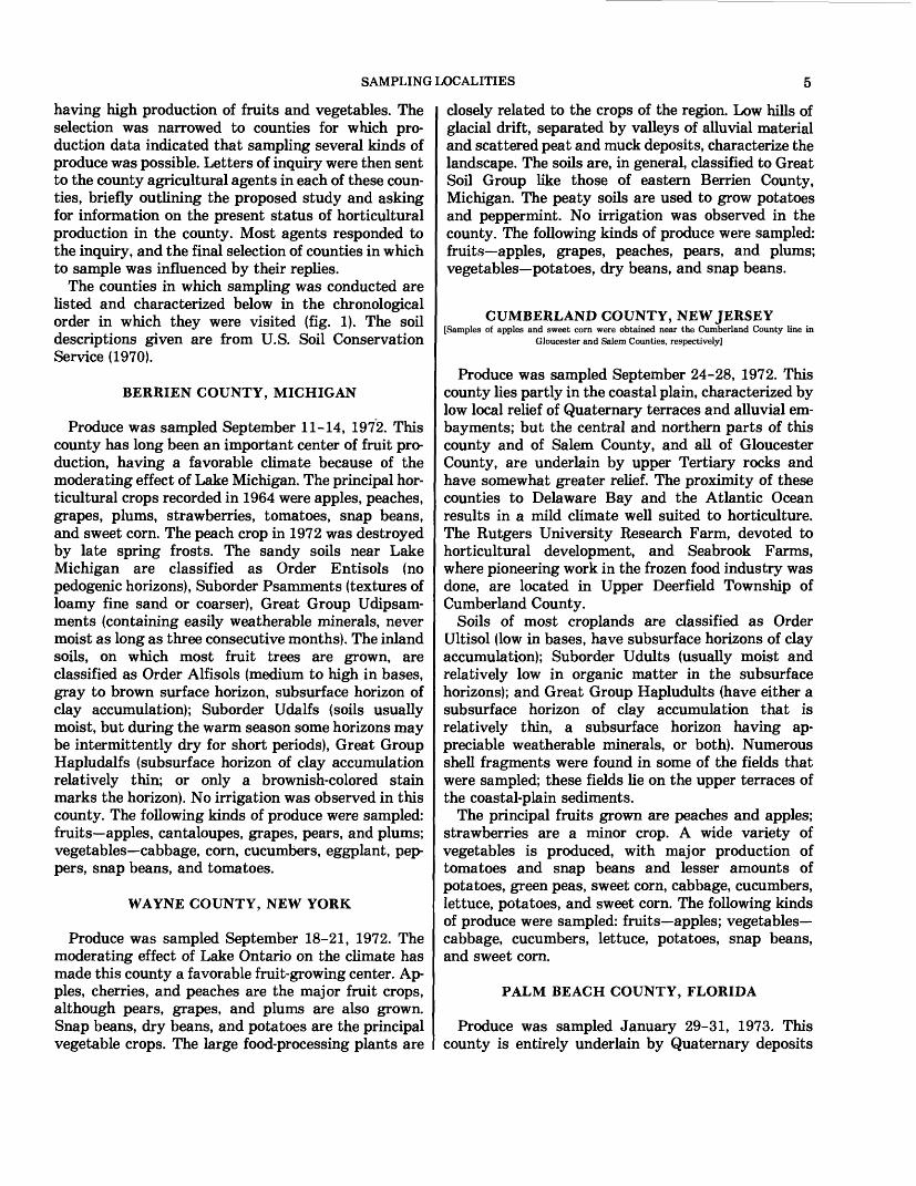
The counties in which sampling was conducted are listed and characterized below in the chronological order in which they were visited (fig. 1). The soil descriptions given are from U.S. Soil Conservation Service (1970).
BERRIEN COUNTY, MICHIGAN
Produce was sampled September 11-14, 1972. This county has long been an important center of fruit pro duction, having a favorable climate because of the moderating effect of Lake Michigan. The principal hor ticultural crops recorded in 1964 were apples, peaches, grapes, plums, strawberries, tomatoes, snap beans, and sweet corn. The peach crop in 1972 was destroyed by late spring frosts. The sandy soils near Lake Michigan are classified as Order Entisols (no pedogenic horizons), Suborder Psamments (textures of loamy fine sand or coarser), Great Group Udipsam- ments (containing easily weatherable minerals, never moist as long as three consecutive months). The inland soils, on which most fruit trees are grown, are classified as Order Alfisols (medium to high in bases, gray to brown surface horizon, subsurface horizon of clay accumulation); Suborder Udalfs (soils usually moist, but during the warm season some horizons may be intermittently dry for short periods), Great Group Hapludalfs (subsurface horizon of clay accumulation relatively thin; or only a brownish-colored stain marks the horizon). No irrigation was observed in this county. The following kinds of produce were sampled: fruits—apples, cantaloupes, grapes, pears, and plums; vegetables—cabbage, corn, cucumbers, eggplant, pep pers, snap beans, and tomatoes.
WAYNE COUNTY, NEW YORK
Produce was sampled September 18-21, 1972. The moderating effect of Lake Ontario on the climate has made this county a favorable fruit-growing center. Ap ples, cherries, and peaches are the major fruit crops, although pears, grapes, and plums are also grown. Snap beans, dry beans, and potatoes are the principal vegetable crops. The large food-processing plants are
closely related to the crops of the region. Low hills of glacial drift, separated by valleys of alluvial material and scattered peat and muck deposits, characterize the landscape. The soils are, in general, classified to Great Soil Group like those of eastern Berrien County, Michigan. The peaty soils are used to grow potatoes and peppermint. No irrigation was observed in the county. The following kinds of produce were sampled: fruits—apples, grapes, peaches, pears, and plums; vegetables—potatoes, dry beans, and snap beans.
CUMBERLAND COUNTY, NEW JERSEY[Samples of apples and sweet corn were obtained near the Cumberland County line in
Gloucester and Salem Counties, respectively]
Produce was sampled September 24-28, 1972. This county lies partly in the coastal plain, characterized by low local relief of Quaternary terraces and alluvial em- bayments; but the central and northern parts of this county and of Salem County, and all of Gloucester County, are underlain by upper Tertiary rocks and have somewhat greater relief. The proximity of these counties to Delaware Bay and the Atlantic Ocean results in a mild climate well suited to horticulture. The Rutgers University Research Farm, devoted to horticultural development, and Seabrook Farms, where pioneering work in the frozen food industry was done, are located in Upper Deerfield Township of Cumberland County.
Soils of most croplands are classified as Order Ultisol (low in bases, have subsurface horizons of clay accumulation); Suborder Udults (usually moist and relatively low in organic matter in the subsurface horizons); and Great Group Hapludults (have either a subsurface horizon of clay accumulation that is relatively thin, a subsurface horizon having ap preciable weatherable minerals, or both). Numerous shell fragments were found in some of the fields that were sampled; these fields lie on the upper terraces of the coastal-plain sediments.
The principal fruits grown are peaches and apples; strawberries are a minor crop. A wide variety of vegetables is produced, with major production of tomatoes and snap beans and lesser amounts of potatoes, green peas, sweet corn, cabbage, cucumbers, lettuce, potatoes, and sweet corn. The following kinds of produce were sampled: fruits—apples; vegetables- cabbage, cucumbers, lettuce, potatoes, snap beans, and sweet corn.
PALM BEACH COUNTY, FLORIDA
Produce was sampled January 29-31, 1973. This county is entirely underlain by Quaternary deposits

ELEMENTS IN FRUITS AND VEGETABLES, CONTERMINOUS UNITED STATES
.COLORADO j i Mesa :
' County
EXPLANATION
• Autumn-harvested produce
D Winter-harvested produce \ n Hidalgo 0 KILOMETERS 400 '"-• County |——,—"—,——rj——,—i____i,——,——,-——j
0 MILES 400
FIGURE 1.—Location of counties where fruits and vegetables were sampled.
(Vernon and Puri, 1964) composed of limestones, shells, clays, and sands. The coastal part is marked by beach terraces of sand and has low relief, whereas most of the county is nearly level and is part of the vast Everglades swamp. Parts of this swamp have been drained, and the deep, highly organic soil now con stitutes excellent land for vegetable production. Numerous drainage canals and ditches divide the land into large flat fields, some of which are planted in sugarcane. No irrigation was observed in this county.
The soils of the sandy terraces are classified as Order Entisols (soils without pedogenic horizons); Suborder Aquents (soils either permanently wet or seasonally wet, have mottled or gray colors); Great Group Psam- maquents (textures of loamy fine sand, or coarser). The soils of the flat lands south and east of Lake Okee- chobee are classified as Order Histosols (wet peat and muck soils). Further classification is based only on the degree of organic-matter decomposition; the soils here have plant residues that are moderately to highly decomposed. The deep organic deposits shake or "vi brate" when walked on; and, since they were drained, oxidation of the organic material has caused a gradual lowering of the land surface.
Citrus fruits (oranges, grapefruit, and lemons) are the only fruits grown commercially. A very large varie ty of vegetables is produced, including beans, cabbage, celery, Chinese cabbage, corn, endive, escarole, lettuce, parsley, peppers, potatoes, radishes, squash, and tomatoes. The three vegetables produced in greatest quantity in 1971-72 were yellow sweet corn, 10,156 carloads; celery, 8,372 carloads; and tomatoes, 3,510 carloads (Robert S. Pryor, County Extension Director, written commun., 1973). The produce of this county is shipped mostly as fresh fruit and vegetables, proc essed foods being limited to citrus concentrates. The following kinds of produce were sampled: fruits- grapefruit and oranges; vegetables—Chinese cabbage, endive, lettuce, parsley, snap beans, sweet corn, and tomatoes.
HIDALGO COUNTY, TEXAS
Produce was sampled February 6-7, 1973. This county generally has a mild winter climate and frosts are uncommon, but a January frost had killed the less resistant vegetables such as tomatoes, peppers, and
SAMPLING LOCALITIES
cucumbers just before this area was sampled. Irriga tion is required for the culture of all fruits and vegetables. The county is underlain by Quaternary deposits of the Lower Rio Grande Valley and the Gulf Coastal Plain. The soils of the lowland near the Rio Grande River are classified as Order Mollisols (black, friable, organic-rich surface horizons high in bases); Suborder Ustolls (Mollisols of semiarid regions; inter mittently dry for a long period, or have subsurface horizons of salt or carbonate accumulation); Great Group Haplustolls (subsurface horizon high in bases but without large accumulations of clay, calcium car bonate, or gypsum). Soils of the northern one third of the county are classified as Order Entisols (without pedogenic horizons), Suborder Psamments (Entisols that have textures of loamy fine sand or coarser), Great Group Ustipsamments (contain easily weather- able minerals; intermittently dry for long periods during the warm season).
The county leads Texas counties in the production of cabbage, cantaloupes, carrots, citrus, cucumbers, broc coli, lettuce, onions, and sweet corn, having 63,900 acres in vegetables alone (A. H. Karcher, Jr., County Agricultural Agent, written commun., 1971). In addi tion to the production listed above, lettuce, potatoes, spinach, tomatoes, and watermelons are also commer cially grown. The following kinds of fruits and vege tables were sampled: fruits—grapefruit and oranges; vegetables—cabbage, carrots, lettuce, and onions.
IMPERIAL COUNTY, CALIFORNIA
Produce was sampled March 2-4, 1973. Most crops of this county are grown on the large plain of Imperial Valley that is below sea level and is irrigated with water from the Colorado River. The climate is warm and dry, and crops are grown in all months of the year. Soils in the valley are composed of silt and clay deposited by flooding of the Colorado River, and soils fringing the valley were largely derived from eolian sands. The valley soils are classified as order Entisols (soils without pedogenic horizons); Suborder Orthents (loamy or clayey, with a regular decrease in organic matter content with depth); Great Group Torrior- thents (Orthents that are never moist as long as three consecutive months).
Imperial County is among the most productive agri cultural counties in the United States. The major vege table crops in 1970-71 were asparagus, cabbage, can taloupes, carrots, cucumbers, lettuce, onions, squash, tomatoes, and watermelons. Of these crops, lettuce was greatest in quantity (444,000 tons) and had a value of $44,795,000 (Imperial County Board of Supervisors, 1971). Citrus crops are limited to relatively few acres
in this county, and the agricultural agent advised sam pling these crops in the Coachella Valley of adjacent Riverside County. The following produce was sampled: fruits—grapefruit and oranges; vegetables—aspara gus, cabbage, lettuce, and carrots.
YUMA COUNTY, ARIZONA
Produce was sampled March 6, 1973. The area from which samples were collected is recently reclaimed desert land in the general vicinity of Hyder. The cultivated land surface is nearly level, is generally free of stones, and is irrigated with ground water. The water is warm as it comes from the wells and, by flowing through ditches in the citrus groves, gives some protection from the occasional frosts. When sam pled, however, the groves showed some frost damage to lemon and orange trees, but little or no damage to grapefruit trees. Anhydrous ammonia is injected into the irrigation water at the wellhead.
The soils are classified as Order Aridisols (with pedogenic horizons low in organic matter and never moist as long as three consecutive months), Suborder Argids (with a horizon of clay accumulation), Great Group Haplargids (with a loamy horizon of clay ac cumulation and with or without alkali). Many citrus groves have been planted recently, and trees in these groves had not reached fruiting age when the area was sampled. Grapefruit and oranges are the principal fruits grown and were the only fruits sampled, although lemons, tangerines, and plums are also grown. No vegetable crops were observed in the area.
TWIN FALLS COUNTY, IDAHO
Produce was sampled September 3-5, 1973. The deep canyon of the Snake River marks the northern boundary of this county, and water from the river enables crops to be grown in this desert area that is underlain by volcanic rocks. Along the river, calcic soils low in organic matter form a narrow band on a plateau that widens to the west and south until ter minated by an abrupt higher plateau having soils richer in organic material. The calcic soils are classified as Order Aridisols (usually dry soils with pedogenic horizons, low in organic matter); Suborder Orthids (Aridisols with accumulations of calcium carbonate, gypsum, or other salts more soluble than gypsum, but having no horizon of clay accumulation); Great Group Calciorthids (Orthids with a horizon in which large amounts of calcium carbonate or gypsum have ac cumulated). The more organic soils of the higher plateau are classified as Order Mollisols (soils with nearly black, organic-rich surface horizons and high
8 ELEMENTS IN FRUITS AND VEGETABLES, CONTERMINOUS UNITED STATES
base supply); suborder Xerols (Mollisols found in climates with rainy winters but dry summers; soils continually dry for long periods in summer), Great Group Agerixerolls (having a relatively thin subsur face horizon of clay accumulation or only a brownish- colored stain to mark this horizon).
The plateau along the river formerly produced apples and other fruits, but most of these orchards have been abandoned. Sweet corn, dry beans, snap beans, and potatoes are now produced in this area. Extensive plantings of potatoes have been developed on the plateau to the south as irrigation was extended to his very dry area. The vegetables sampled were dry beans, snap beans, sweet corn, and potatoes.
YAKIMA COUNTY, WASHINGTON
Produce was sampled September 7-10, 1973. This county was reported to rank first among counties of the State in value of all agricultural products, and was also first in fruit and vegetable production. It led all counties in the United States in apple and pear produc tion (Washington State Department of Agriculture, 1964). The horticultural crops are produced on the broad alluvial plains and terraces that lie adjacent to the Yakima River and its tributaries and are irrigated with water from these streams. The county has a con tinental climate which is hot and dry in the summer and relatively mild and moist in the winter. The prin cipal soils used for fruit and vegetable growing are alluvial soils of fine silty and sandy loams mixed with fine volcanic ash. Fruit production is centered on the higher terraces where spring frost damage is reduced, whereas vegetables and some specialized crops (hops and mint) are grown on the lower lands.
Soils of the Yakima Valley are classified as Aridisols (soils with pedogenic horizons, low in organic matter, usually dry), Suborder Orthids (having a horizon of clay accumulation with or without alkali); Great Group Haplargids (having a loamy horizon of clay accumula tion). The principal fruits grown are apples, apricots, berries, cherries, grapes, peaches, and plums. Vege tables, ranked in order of number of acres in produc tion, are sweet corn, asparagus, green peas, tomatoes, cantaloupes, rutabagas and turnips, watermelons, onions, carrots, lettuce, cucumbers, and spinach. Food processing constitutes an important industry in the county, and some crops are sold both as fresh and as canned or frozen produce. The following kinds of produce were sampled: fruits—apples, American and European grapes, peaches, pears, and plums; vege tables—potatoes and tomatoes.
SAN JOAQUIN COUNTY, CALIFORNIA
Produce was sampled September 14-17, 1973. The principal agricultural lands lie in the alluvial plain of the San Joaquin River, where a large variety of fruits and vegetables, as well as other crops and livestock, is produced. The horticultual crops are sold both as fresh and as processed foods. Rainfall amounts are usually low, occurring mostly in winter; therefore, irrigation is necessary for most crops. Azonal loamy or clayey alluvial soils predominate along the river; these soils are classified as Order Entisols (soils having no pedogenic horizons); Suborder Orthents (loamy or clayey, and having a regular decrease in organic- matter content with depth); Great Group Xerorthents (Orthents in climates with rainy winters but dry sum mers; continually dry for long periods during the warm season). Adjacent, but higher, areas have soils that are high in bases and have clayey horizons. These soils are classified as Order Alfisols (medium to high in bases, with gray to brown surface horizons and subsurface horizons of clay accumulation); Suborder Udalfs (soils usually moist, but may be intermittently dry in some horizons); Great Group Hapludalfs (soils with subsur face horizon of clay accumulations that is relatively thin, or having only a brownish-colored stain to mark this horizon). A small area at the northwestern tip of the county has wet organic soils; this area was not sampled.
The fruits that are grown include apples, apricots, cherries, grapes, nectarines, olives, peaches, pears, plums, and strawberries. Of these fruits, grapes and cherries are among the county's 10 leading crops in value. Tomatoes and asparagus are also among these leading crops; and, in addition, snap beans, lima beans, cabbage, carrots, cauliflower, sweet corn, cucumbers, lettuce, melons, onions, peas, peppers, potatoes, pump kins, squash, sweet potatoes, beets, and spinach, listed in order of quantity that is produced, are commercially grown (Stipe and Jones, 1972). The following kinds of produce were sampled: fruits—European grapes, peaches, and pears; vegetables—cucumbers, dry beans, and tomatoes.
MESA COUNTY, COLORADO
Produce was sampled September 22-24, 1973. This area is one of the few in the Rocky Mountain region in which occurs significant production of fruits and some vegetables; total production here, however, is small compared to that of other areas that were sampled. The cultivated lands lie along the Colorado and Gun- nison Rivers and tributary streams where water is
METHODS OF SAMPLING PLANTS AND SOILS
available for irrigation. Field crops and vegetables are grown in the low alluvial soils, and fruits are mostly on higher ground. The soils are classified as Order En- tisols (soils without pedogenic horizons) but fall into two Suborders, Fluvents and Orthents. The Fluvents (Entisols having organic-matter content decreasing ir regularly with depth; formed in loamy or clayey alluvial deposits) are further classified to Great Group Torrifluvents (never moist as long as three consecutive months). Soils of Suborder Orthents (loamy or clayey Entisols that have a regular decrease in organic-matter content with depth) are further classified as Tor- riorthents (never moist as long as three consecutive months). The following produce was sampled: fruits- apples, peaches, pears, and plums; vegetable—dry beans.
METHODS OF SAMPLING PLANTS AND SOILS
SAMPLING DESIGN
Only one trip to each area of food-plant production was practical because of restrictions of time and resources. Organization of the sampling plan, there fore, required first an estimate of the major harvest times for the several areas to be sampled in order to maximize the opportunity of obtaining different kinds of produce during the one visit to each area. Autumn harvest was selected as the most important harvest for the northern localities, the spring and early summer crops being generally less important. This selection, however, eliminated the berry crops, cherries, and some early summer vegetables from the sampling targets in the northern areas. In the southern localities the harvest is spread more uniformly throughout the year, particularly in areas where several crops of a vegetable can be grown in a single year. The tree fruit crops are more seasonal, being generally harvested during the winter months; therefore the winter harvest season was selected for the southern localities (fig. 1), although the hazard of frost damage occurs at this season.
Counties in eleven areas of fruit and vegetable pro duction were selected for sampling (fig. 1). Within each area the sampling plan required the selection of five fields in which a particular crop was grown. This selec tion was based on a general reconnaissance of the area before sampling was begun, often with the recommen dations of the county agricultural agent as guides, in order to locate potential sampling targets for each kind of produce. Formal random selection of fields was seldom possible: some fields had already been har
vested; some were not yet mature; and, for some, permission to sample could not be obtained, generally because the owner of the land could not be located. Fields were sampled, therefore, as the opportunity arose.
Within each field (or grove, orchard, vineyard, or plot), two sites were selected for sampling produce by quartering the field into successively smaller units by drawing lots until a sampling site (variously defined as a single tree, a vine, a clump, or a row) was chosen. At this site an adequate sample of the fruit or vegetable was collected. Duplicate samples of produce were col lected at about 10 percent of the sites, as dictated by a randomization procedure developed before field work was begun by generating a block of random numbers from 1 to 1,000 and ordering them into numerical se quence by a computer program. As sites were sampled they were numbered consecutively, and at the site whose sequential number corresponded to the next se quential random number a duplicate sample of plant material was obtained. These duplicate samples were collected in order to determine the variance in geochemical properties within a site. Soil was sampled at only one field within each area for each type of produce.
After all samples had been dried and pulverized, about 10 percent of the samples (45) were split (divided into approximate halves), again selecting by random numbers generated similarly, but not identically, to the random numbers described above. This procedure enabled an estimation of laboratory and analytical error to be made by a comparison of the analytical values reported for each pair of samples.
All prepared samples of plant material and soils, in cluding field duplicates and laboratory splits, were ar ranged in a randomized order that was unknown to the analysts and were then submitted to the analytical laboratories. This procedure minimizes the effects of variable operator bias and analytical drift on inter pretation of the data.
The hierarchical organization of sampling the kinds of produce can be outlined as follows:Two to five areas, depending on the produce (counties in 10 different
States)Five fields per area
Two randomly selected sites per field Duplicate samples at 45 randomly selected sites
Laboratory splits of 45 randomly selected samples.The duplicate samples at 45 sites and the 45
laboratory splits did not include all kinds of produce that were studied because of their random selection from the entire lot of sites and samples. Analyses of these samples, therefore, provide general estimates of chemical variation and sampling error within sites, and laboratory error in sample preparation and analysis.
10 ELEMENTS IN FRUITS AND VEGETABLES, CONTERMINOUS UNITED STATES
SAMPLING TECHNIQUES
SPECIES OF PLANTS SAMPLED
It was not possible to sample the cultivar of a species at all sampling localties where the species was cultivated, because the cultivars that are grown com mercially in a particular area are those that are especially adapted to the climate, cultivation prac tices, and market preferences of the area. Although some studies have shown that different cultivars of certain species differ in concentrations of particular elements in edible parts of the plants, other studies have found only slight, or no, differences among cultivars of other species. (See discussion by Beeson, 1941.) If differences do exist among some cultivars sampled in this study, the summary data given for cer tain elements in a fruit or vegetable in a locality and in the United States will be biased to an unknown extent. From an overall dietary viewpoint, however, if these differences exist they probably are of minor impor tance, assuming that the produce actually sampled is representative of these foods as consumed by a large percentage of the population.
The common and scientific names of species, and the names (if known) and numbers of cultivars (cv.) that were sampled, are given for each locality in the list that follows. Field replicate samples, if collected, are in cluded. The areas are listed in order of sampling.
FRUITS
American grape, Vitis labruscana Bailey. The species name is a hor ticultural name for the group of cultivars originating from a wild grape, V. labrusca L., that is native to North America. Cultivars included in this group are Concord, Catawba, Niagara, and others. These cultivars can be distinguished from those of the European grape (V. vinifera L.) by the "skin" on the berry easily slipping from the pulp within, whereas the skin adheres to the pulp in the European species. Berrien County, Mich.—cv. Concord, 12. Wayne County, N.Y.—cv. Niagara, 7; Catawba, 2. Yakima County, Wash.—cv. Concord, 10. These grapes are eaten fresh and are also processed as juice, preserves, and wine.
Apple, Pyrus malus L. Two groups are recognized, summer harvested and autumn harvested; the following samples were of autumn-harvested cultivars. Berrien County, Mich.—cv. Russet, 1; cv. Stay man (also called Stay man Winesap), 9. Wayne County, N.Y.—cv. Greening, 6; cv. Golden Delicious, 4. Gloucester County, N.J.—cv. Red Delicious, 6; cv. Greening, 2. Yakima County, Wash.—cv. Red Delicious, 6; cv. Standard Delicious, 4. Mesa County, Colo.—cv. Red Delicious, 10.
Cantaloupe, Cucumis melo L. Cantaloupe is classified in some pro duction reports as a vegetable. It was sampled only in Berrien County, Mich.—cv. unknown, 2. It was not found with mature fruits in other areas when sampling was conducted.
European grape, Vitis vinifera L. This grape has been in cultivation in Europe and Asia Minor since ancient times. Two groups are
recognized within this species, table grapes and wine grapes, de pending on the principal use of the fruit. Only cultivars com monly known as table grapes were sampled; some of these, however, are also used in wine making. The European grape is commercially grown in this country mostly in the Pacific Coast States, principally in California. Yakima County, Wash.—cv. Thompson Seedless, 5 (a very sweet grape that is also dried and used as raisins); cv. Black Mahukka, 4; cv. Palomino, 2. San Joa- quin County, Calif.—cv. Tokay, 10.
Grapefruit, Citrus parodist Sw. Two principal groups were recog nized in the trade, the red- or pink-pulp cultivars and the yellow- pulp cultivars. Fruits in both groups are eaten fresh, canned, or used as frozen juice concentrate. Palm Beach County, Fla.—cv. Marsh Seedless, 10. Hidalgo County, Tex.—cv. Ruby Red, 8; cv. unknown (yellow pulp), 10. Riverside County, Calif.—cv. unknown (yellow pulp), 10. Yuma County, Ariz.—cv. Ruby Red, 9; cv. unknown (yellow pulp), 1.
Orange, Citrus sinesis Osbeck. Most commercial oranges are cultivars of this species. The King orange (generally sold as fresh fruit) is, however, a cultivar of Citrus nobilis Lour. The Mandarin orange, usually sold as canned fruit of oriental origin, is Citrus nobilis var. deliciosa Sw. All samples are cultivars of the Citrus sinensis species, of which two groups, fresh-fruit cultivars and juice cultivars, are recognized in the trade ac cording to the predominant use of the fruit. Palm Beach Coun ty, Fla.—cv. Valencia, 11. Hidalgo County, Tex.—cv. Valencia, 10. Riverside County, Calif.— cv. Valencia, 10. Yuma County, Ariz.—cv. Valencia, 11.
Peach, Prunus persica Batsch. Two groups are recognized, freestone and clingstone, the first having flesh that separates easily from the stone, in contrast to the adhering flesh of the second. Although both kinds are canned, the clingstone with its firmer flesh is more commonly processed in this manner. Cling stone cultivars are not usually sold as fresh fruits, except some early-season kinds. Most commercial peaches are yellow-flesh cultivars, but white-flesh cultivars are grown to a limited extent for pickles or are sold as fresh fruit. Wayne County, N.Y.—cv. Early Elberta (freestone), 5; cv. Elberta (freestone), 2; cv. Hale (freestone), 2. Yakima County, Wash.—cv. Hale (freestone), 10. San Joaquin County, Calif.—cv. Halford (clingstone), 10.
Pear, Pyrus communis L. Pears are sold fresh and canned, and for both uses the fruit of the Bartlett cultivar is the most im portant. The cultivar Kieffer, generally used canned or pre served, is supposed to be a chance hybrid of the Bartlett cul tivar and the Chinese sand pear, Pyrus serotina Rehd. Berrien County, Mich.—cv. Bartlett, 7; cv. Kieffer, 3. Wayne County, N.Y.—cv. Bartlett, 7; cv. Seckel, 2; cv. Bosc, 2. Yakima County, Wash.—cv. D'Anjou, 10. San Joaquin County, Calif.—cv. Bartlett, 10. Mesa County, Colo.—cv. Bartlett, 12.
Plum, Prunus domes tica L. The large purple plums, often partly freestone, that are eaten fresh, canned, or dried as prunes, belong to this European species, as does the Green Gage cultivar that is commonly used fresh, but occasionally is canned. The yellow and red plums sold as fresh fruit generally are cultivars of an Asiatic plum, Prunus salicina L., or are hy brids of this plum and some American species such as Prunus americana Marsh, Prunus hortulana Bailey, and others. Dam son, the small purple plum used largely for preserves, is con sidered here as a Prunus domes tica cultivar, although some writers assign it to Prunus institia L. All plums reported here are cultivars of the European species. Berrien County, Mich.—cv. Stanley, 4; cv. Bluefree, 2; cv. Damson, 4. Wayne County, N.Y.—cv. Stanley, 10. Yakima County, Wash.—cv. Italian, 11. Mesa County, Colo.—cv. Italian, 10.

METHODS OF SAMPLING PLANTS AND SOILS 11
VEGETABLES
Asparagus, Asparagus officinalis L. Asparagus was sampled in only one locality, Riverside County, Calif.—cv. unknown, 10. Although it is extensively grown in Yakima County, Wash, and San Joaquin County, Cah'f., the harvest period of this vegetable generally is March to May, and these counties were not visited during this period.
Cabbage, Brassica oleracea var. capitata L. Two color types are recognized, the common green cabbage which was sampled, and the red cabbage. Cabbage cultivars are assigned to three groups on the basis of time of maturation: early (having either pointed or spheroid heads), midseason (generally having spheroid heads), and late (having spheroid or flattened-spheroid heads). Only spheroid (commonly called "round")-head cultivars were sampled. The group of cultivars having crinkled leaves that is designated savoy cabbage was not sampled. Commercially, cab bages are classified as either fresh or processing kinds, the lat ter being made up as sauerkraut. Berrien County, Mich.—cv. unknown, 3. Cumberland County, N.J.,—cv. unknown, 2. Hidalgo County, Texas—cv. unknown, 12. Imperial County, Calif.—cv. unknown (a processing kind), 11.
Carrot, Daucus carota L. Carrots are classified commercially as fresh market or processing, depending on the method of marketing. All samples were cultivars having long taproots. Hidalgo County, Texas—cv. unknown, 10. Imperial County, Calif.—cv. unknown, 11.
Chinese cabbage, Brassica pekinesis (Luor.) Ruprecht. Chinese cab bage was found only in Palm Beach County, Fla.—cv. unknown, 3.
Cucumber, Cucumis sativus L. Cultivars are grouped into slicing and pickling kinds, the former being generally longer and larger than the latter. Fruits of slicing cultivars are sometimes pickled either when young and small, or when more mature and larger. Small pickles of this species may be sold as gherkins; this name, however, is more properly applied to Cucumis anguria L., the West Indian gherkin, which has fruits that are spiny and 2-4 cm long. Berrien County, Mich.—cv. unknown, 10. Cumber land County, N.J.—cv. unknown, 2. San Joaquin County, Calif.—cv. unknown, 10.
Dry beans, Phaseolus vulgaris L. Many cultivars of beans have originated, principally by natural mutations, from this species. Those grown for their dry seeds form a group that is distinguished from the cultivars having pods that are edible when immature (snap beans), although seeds of both types can be eaten as dry beans. Most production reports classify dry beans as field crops rather than as vegetables. Wayne County, N.Y.—cv. Red Kidney, 7; cv. Yellow Eye (used in canned soups and "pork and beans"), 4. Twin Falls County, Idaho—cv. Light Red Kidney, 4; cv. Red Kidney, 2; cv. Pinto, 4. San Joaquin County, Calif.—cv. Red Kidney, 11. Mesa County, Colo.—cv. Pinto, 10.
Endive, Cichorium endivia L. Endive is a leafy salad vegetable of minor commercial importance. Palm Beach County, Fla.—cv. Green Curled, 2.
Eggplant, Solanum melongena L. Only the large, ovate, purple- fruited kinds are commonly grown in this country. Berrien County, Mich.—cv. unknown, but probably an F, hybrid of the Black Beauty type, 3.
Lettuce, Lactuca sativa var. capitata L. Head lettuce, the only kind sampled, is by far the most important kind produced com mercially, although leaf, curled, cos, and romaine cultivars are widely grown. Cumberland County, N.J.—cv. "659," 10. Palm
Beach County, Fla.—cv. Iceberg type, 10. Hidalgo County, Tex.—cv. Iceberg type, 10. Imperial County, Calif.—cv. Iceberg type, 10.
Onion, Allium cepa L. Only the type grown for bulbs was sampled, although young plants of the bulb type are at places thinned from the rows and sold as green or bunched onions, while the re maining wider spaced plants are left to produce bulbs. Some cultivars, in contrast, do not form bulbs of marketable quality and are grown for sale only as bunching onions. Hidalgo Coun ty, Tex.—cv. unknown (white skin type), 10.
Parsely, Petroselinum crispum (Mill.) Nym. Although considered a vegetable of minor commercial importance, Palm Beach County produced 331 railroad carloads in 1971-72 (R. S. Pryor, County Agricultural Agent, written commun., 1972). Palm Beach Coun ty, Fla.—cv. Curled, 2.
Pepper, Capsicum frutescens var. grossum Bailey. These peppers are the large-fruited types commonly called bell peppers, sweet peppers, and pimiento peppers that are green when young but turn bright red when mature. Berrien County, Mich.—cv. California Wonder, 2.
Potato, Solanum tuberosum L. This potato is often called Irish or white potato to distinguish it from sweet potato, Ipomea batatas(L.) Poir. Some production reports classify potatoes as a field crop rather than as a vegetable. The many commercially grown cultivars are of two kinds, russet and red. Russet cultivars that are large and elongated are designated in the trade as baking potatoes. Wayne County, N.Y.—cv. unknown (russet type), 11. Cumberland County, N.J.—cv. unknown (russet type), 11. Twin Falls County, Idaho—cv. unknown (russet baking type), 10. Yakima County, Wash.—cv. unknown (red type), 5; cv. unknown (russet type), 6.
Snap bean, Phaseolus vulgaris L. Commercial usage favors this common name rather than green bean or string bean. Cultivars are of two types, the green pod and the yellow pod or wax. Ber rien County, Mich.—cv. unknown (green type), 2. Wayne Coun ty, N.Y.—cv. unknown (green type), 11. Cumberland County, N.J.—cv. unknown (green type), 11; cv. Yellow Wax, 2. Palm Beach County, Fla.—cv. unknown (green type), 10. Twin Falls County, Idaho—cv. Sprite (green type), 10.
Sweet corn, Zea mays var. rugosa Bonaf. Most commercially grown cultivars of sweet corn are F, hybrids, and field identification of these cultivars is not practical. They are of two types, yellow and white, the former being more widely grown as hybrids related to the Golden Bantam cultivar. Berrien County, Mich.—cv. unknown (yellow), 5. Salem County, N.J.—cv. unknown (yellow), 4; cv. Silver Queen (white), 7. Palm Beach County, Fla.—cv. unknown (yellow), 10. Twin Falls County, Idaho—cv. unknown (yellow), 11.
Tomato, Lycopersicum escutentumMSi. The two commercial groups of tomatoes are shipping (for eating as fresh fruits) and proc essing. Mechanized harvesting has led to the development of fruits, especially of processing cultivars, that are thick skinned, firm, and spherical to cylindrical in shape. Berrien County, Mich.—cv. unknown (shipping), 10. Cumberland County, N.J.—cv. unknown (shipping), 3. Palm Beach County, Fla.—cv. Floridel (shipping), 10. Yakima County, Wash.—cv. unknown (processing), 12. San Joaquin County, Calif.—cv. unknown (processing), 11.
COLLECTION AND PREPARATION OF SAMPLES
Samples at a site were subjectively sampled from the tree, vine, or row of produce with the intent of ob taining samples representative of the produce as it is
12 ELEMENTS IN FRUITS AND VEGETABLES, CONTERMINOUS UNITED STATES
selected for marketing or processing. Factors used in the selection included degree of maturity, size, shape, freedom from large blemishes, and coloration, as ap propriate for the kind of produce being sampled. The fruit and vegetables were placed in plastic bags at the collection site in order to reduce loss of their field moisture content; at the end of the same day they were prepared as for eating or cooking (but were not cooked), and the prepared samples were weighed to 0.1 g. Samples were then heat-sealed in thick polyeth ylene bags, packed in ice chests to reduce spoilage, and as soon as possible shipped by air mail to the Denver laboratories where they were frozen and held until dry ing could be started.
Methods used to prepare the various kinds of samples are listed below:
FRUITS
American grape. Bunches washed and drained, berries removedfrom stems, skins and seeds included in sample.
Apple. Fruit washed and drained, fruit peeled, core removed, fruitsliced.
Cantaloupe. Fruit peeled, seeds removed, flesh sliced and cubed. European grape. Fruit washed and drained, fruit cut open, seeds
removed. Grapefruit. Fruit peeled, segments separated and cut into pieces,
seeds discarded.Orange. Fruit prepared the same as for grapefruit. Peach. Fruit peeled, seed (pit) removed, fruit sliced. Pear. Fruit peeled, core removed, fruit sliced. Plum. Fruit washed and drained, seed (pit) removed, fruit sliced.
VEGETABLES
Asparagus. Stalks washed and drained, cut into segments; toughstalks discarded.
Cabbage. Outer leaves removed and discarded; firm head washedand drained, then sliced.
Carrot. Leafy tops removed; root washed, drained, peeled, sliced. Cucumber. Fruits washed and drained, not peeled, sliced. Dry bean. Seeds removed from dry pods and winnowed to remove
foreign material; molded or imperfect seeds discarded. Endive. Leaves washed and drained, cut into pieces. Eggplant. Fruit peeled and sliced. Lettuce. Heads washed and drained, outer leaves removed to firm
head, head sliced.Onion. Tops, roots, and dry leaf bases removed; bulb sliced. Parsley. Leaves washed and drained. Pepper. Fruits washed, seeds and their supporting tissues removed,
fruit sliced.Potato. Tubers washed and drained, peeled, sliced. Snap bean. Pods washed and drained, stems and tips removed, pods
broken into pieces. Sweet corn. Shucks (husks) and silks (styles) removed, grains cut
from the cob (rachis), cob discarded. Tomato. Fruits washed and drained, sliced.
In the preparation laboratory, the plastic bags con taining the frozen individual samples were opened wide and placed in shallow aluminum pans which were put into an electric oven that had circulating air held at a temperature of 38-40° C. By following this pro cedure, the samples were prevented from contacting the aluminum pan. Several days later the samples that appeared dry were removed from the oven and weighed to 0.1 g. They were then returned to the oven where they remained 1 day, then they were weighed again. This process was continued until no further loss in weight occured; the dry samples were then sealed in polyethylene bags. Leafy samples (for example, lettuce and cabbage) and those with a high starch content (for example, potatoes and corn) dried to a constant weight in 3-5 days, whereas samples with a high sugar con tent (peaches and grapes), rich in colloids (cucumbers), or with a high water content (tomatoes) required as much as 2 weeks of drying to attain a constant weight.
The dried samples were pulverized or shredded in a Waring blender1 that had a glass canister and stainless steel blades. The blender was cleaned after grinding each sample, either by blowing it out with compressed air or by washing it, as necessary. Certain randomly selected samples, as described earlier, were divided into two parts; then all ground samples were placed in covered cardboard cartons. After grinding the plant materials the particles were of a size that would pass through a screen with apertures of 1.3 mm.
SOILS
A sample of soil was collected at each site where pro duce was sampled by digging to the lower limit (usu ally 15-20 cm from the surface) of the plow zone, then taking a composite sample of the soil that was re moved. The soil had been cultivated at all sampling sites; therefore, there had been some mixing of soil horizons in zonal soils. The samples were placed in manila soil envelopes and allowed to dry at ambient air temperatures until they were finally dried in the laboratory at 38-40° C. A Nasco-Asplin soil grinder equipped with a ceramic mortar, ceramic screw-type grinding head, and stainless steel screen was used to gently break up the soil aggregates and to separate and discard large roots and soil material (mostly gravel) larger than 2 mm. The fine material was then ground in a vertical Braun pulverizer using ceramic plates set to pass 80 mesh. The samples were then ar ranged in a random sequence and submitted to the laboratory for chemical analysis.
'Use of brand names in this report is for descriptive purposes only and does not con stitute endorsement by the U.S. Geological Survey.
STATISTICAL PROCEDURES USED IN EVALUATING DATA 13
ANALYTICAL METHODS USED
PLANTS
A part of each dried and pulverized sample of fruits and vegetables was burned to ash in a furnace which was slowly heated from room temperature to 500 ° C, and the weight percent of ash produced from the dried material was recorded. The ash was used for analysis by the emission spectrographic method (Neiman, 1976) and for the determination of cadmium, cobalt, zinc, sodium, lithium, calcium, potassium, and phosphorus using methods described by Harms (1976). Dried plant material was used for analysis of arsenic, mercury, selenium, and total sulfur. The methods of analysis us ed for determining the various elements in the plant material, and the lower limit of determination, are given in table 1.
SOILSFor analysis by emission spectroscopy, a 10-mg ali
quot of each soil sample was mixed with 20 mg of a sodium carbonate-graphite mixture (1 percent Na), then packed into a shallow crater electrode and burned for 2 minutes in a direct current arc. The resulting spectra were recorded on a photographic plate which was developed and visually compared to reference standards. The preparation of these standards and the method of reporting values were described by Neiman (1976). Procedures used for the analysis of soil samples by atomic absorption, X-ray fluorescence, and certain methods other than emission spectroscopy were de scribed by Huffman and Dinnin (1976) and Wahlberg (1976). Millard (1975) described the delayed neutron technique used for determining thorium and uranium concentrations in soils. All methods used for deter mining the various elements in soils, and the lower limits of determination, are listed in table 2.
STATISTICAL PROCEDURES USED IN EVALUATING DATA
Frequency distributions of the analytical data as received from the laboratory, in units of weight per cent or parts per million, show large positive skewness. In order to achieve frequency distributions more near ly symmetrical and closer to the normal form, the original data were transformed to logarithms. Many of the elements were analyzed by a semiquantitative spectrographic method for which the concentrations were reported in geometric brackets; log transforma tion also overcomes some of the effects of this method of reporting on evaluation of the data (Miesch, 1967).
The geometric mean is the appropriate measure of central tendency for a lognormal distribution and pro vides a "characteristic" value for the element in the sampling media. The geometric mean is estimated as the antilog of the arithmetic mean of the logs. A measure of variation is given by the geometric devia tion, which is the antilog of the standard deviation of the logs. About two thirds of the area under the log- normal distribution curve lies in the range GM+GDto GMX GD, where GM is the geometric mean and GD is the geometric deviation. The confidence interval about the geometric mean, the geometric error (GE), can be estimated from
(1)
where t is Student's t and AT is the number of values on which the geometric mean is based. Where t is selected at the 0.05 probability level, the population geometric mean has the expected range GM+GE to GMXGE, with 95 percent confidence (Shacklette and others, 1970).
Because of the insufficient sensitivity of some analytical methods, some elements were not detected in measurable concentrations in many samples of plant tissue or soil. This deficiency resulted in some values being reported as "less than" (<) a specified limit. Such data are said to be censored, and the means and deviations were computed using the procedures de vised by Cohen (1959) and applied to geochemical data by Miesch (1976). Some of the data for a particular ele ment in a plant or soil sample was so severely censored that Cohen' s technique was unreliable or impossible, and the mean is listed in the tables that follow only as "less than" a stated limiting value. The estimated means of censored data are commonly below the stated lower limit of determination, as given in tables 1 and 2.
The total chemical variation within any one type of produce has been viewed as the sum of three com ponents: (1) the variability among the widely separated areas, (2) the variability among fields within an area, and (3) the variability due to all other causes including natural variability within fields and variability that arises from sample preparation and analysis. The cor responding analysis-of-variance model is
where n is the grand mean concentration for all areas, «i is the difference between n and the mean for the ith area, fa j is the difference between n+cti and the meanfor the jth field in the ith area, and T^ is the difference between n+oii+fiij and the log analytical value for the

14 ELEMENTS IN FRUITS AND VEGETABLES, CONTERMINOUS UNITED STATES
TABLE L—Summary of methods used for analysis of plants and plant ashes and approximate lower limits ofdeterminations
Element MethodSample weight
(g)
Lower limit (ppm)
Dry material of sample
As-——— Atomic absorption (arsine generation) 1Hg—--- Flameless atomic absorption————-- 1Se-——— 2, 3-diaminonaphthalene-—— — ---— 2S, total Turbidometric-- —— ——————————— - .5
0.05.01.005
100
Ash of sample
Ag——— Emission spectroscopy-Al——— ————————————do-B———— ————————————do--Ba——— ———————————-do--Ca——— Atomic absorption——-
Cd——— ———————————do- Co——— ———————————do-Cr---— Emission spectroscopy-Cu——— ———————————do-Fe——— ——————————do—
Ga——— ————————————do-K------- Atomic absorption-----La——— Emission spectroscopy-Li——— Atomic absorption-----Mg—--- Emission spectroscopy-
Mn---— -- ——— ——— — ---do- Mo——— ———————————-do— Na-—-- Atomic absorption----- Ni——— - Emission spectroscopy- p——___ Colorimetric--- —— --•
Pb———- Emission spectroscopy-Sn------ - — - —— -_-______do--Sr——— ———————————-do—Ti——— ————.....____.. do-V——- — _—__-—_____d0"
Y——- ............. _—-do--Yb—— ——————do-Zn——-- Atomic absorption- — •Zr——— Emission spectroscopy-
1.01 .01 .01 .01 .05
.5
.5
.01
.01
.01
.01
.05
.01
.05
.01
.01
.01
.05
.01
.05
.01
.01
.01
.01
.01
.01
.01
.05
.01
1150503
100
11,1
10
10100704
20
17
2510
100
2010105
15
202
1020
From Harms (1976) and Neiman (1976).
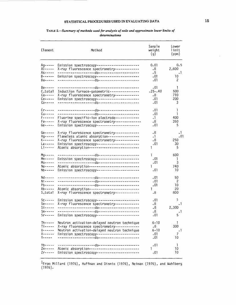
STATISTICAL PROCEDURES USED IN EVALUATING DATA 15
TABLE 2.— Summary of methods used for analysis of soils and approximate lower limits of determinations
Sample Lower Element Method weight limit
(g) (ppm)
Ag- — — Emission spectroscopy--- — -- ———— ——— --- 0.01 0.5Al — -- X-ray fluorescence spectrometry ——— --- — - .8 2,600As ——— ————————————— do —————————————— .5 .1B — — Emission spectroscopy ——— -- ———— — —— - .01 10Ba ——— ————————————— do —————————————— .01 2
Be ——— ————————————— do —————————————— .01 1C, total Induction furnace-gasometric- ——— --- — --- .25-. 40 500Ca----- X-ray fluorescence spectrometry-- ——— — — .8 710Ce----- Emission spectroscopy- — ---- ————— -- — - .01 200Co ——— ————————————— do —————————————— .01 3
Cr ——— ————————————— do —————————————— .01 1Cu ——— ————————————— do —————————————— .01 1F- ——— Fluorine specific-ion electrode- ——— ———— .1 400Fe — -- X-ray fluorescence spectrometry---- ——— — -- .8 350Ga- —— Emission spectroscopy ——— — —— —— — — - .01 5
Ge-- — X-ray fluorescence spectrometry-- ——— — --- .8 .1Hg--_-_ Flameless atomic absorption-- — —— -- — — .1 .01K —— __ X-ray fluorescence spectrometry — ——— ——— .8 250La ——— Emission spectroscopy------- —— -- — ------- .01 30Li----- Atomic absorption — ——— ———— ——— — --- 1 5
Mg ——— ————————————— do —————————————— 1 600Mn ——— Emission spectroscopy ——————— —— —— — .01 1Mo ——— ————————————— do —————————————— .01 3Na ——— Atomic absorption-- —— ———————— —— — - 1 740Nb- —— Emission spectroscopy-- — — ——— — ---- — .01 10
Nd ——— ————————————— do —————————————— .01 50Ni ——— ————— - ———— --do —————— - ——————— .01 2Pb ——— ————————————— do —————— - ——————— .01 10Rb- — - Atomic absorption- ——— -- — ------ ——— —— - 1 20S, total X-ray fluorescence spectrometry ————— — - .8 800
Sc- —— Emission spectroscopy------ — —— — — ---- .01 5Se-- — X-ray fluorescence spectrometry--- ——— - — .8 .1Si ——— ————— _-- ————— do — - —— --- —— --- —— .8 2,300Sn ——— ————————————— do —————————————— .8 .1Sr — -- Emission spectroscopy —— ----- ——— —— ---- .01 5
Th — -- Neutron activation-delayed neutron technique 6-10 1Ti- —— X-ray fluorescence spectrometry--- ——— —— - .8 300U — — Neutron activation-delayed neutron technique 6-10 .1V ——— Emission spectroscopy-------- —— -- ——— — - .01 7y ——— ———————————— -do—- ————————— - —— .01 10
Yb ——— ——————— --- — --do ——————— - ———— -- .01 1Zn----- Atomic absorption ——— ———— ___-_- ———— _ i 10Zr- —— Emission spectroscopy ————— ______ — — __ .01 10
Mil lard (1976), Huffman and Dinnin (1976), Neiman (1976), and Wahlberg (1976).
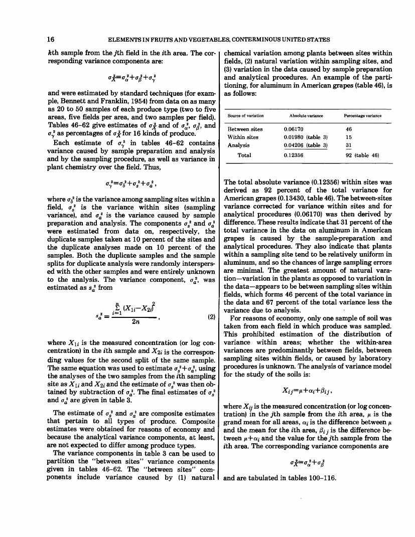
16 ELEMENTS IN FRUITS AND VEGETABLES, CONTERMINOUS UNITED STATES
fcth sample from the jth field in the ith area. The cor- | responding variance components are:
and were estimated by standard techniques (for exam ple, Bennett and Franklin, 1954) from data on as many as 20 to 50 samples of each produce type (two to five areas, five fields per area, and two samples per field). Tables 46-62 give estimates of a£ and of aa2, 0$, and aT2 as percentages of a£ for 16 kinds of produce.
Each estimate of aj in tables 46-62 contains variance caused by sample preparation and analysis and by the sampling procedure, as well as variance in plant chemistry over the field. Thus,
where a52 is the variance among sampling sites within a field, as2 is the variance within sites (sampling variance), and a02 is the variance caused by sample preparation and analysis. The components as2 and a02 were estimated from data on, respectively, the duplicate samples taken at 10 percent of the sites and the duplicate analyses made on 10 percent of the samples. Both the duplicate samples and the sample splits for duplicate analysis were randomly interspers ed with the other samples and were entirely unknown to the analysis. The variance component, a02 , wasestimated as s02 from
2n (2)
where Xu is the measured concentration (or log con centration) in the ith sample and X^i is the correspon ding values for the second split of the same sample. The same equation was used to estimate a*+o£, using the analyses of the two samples from the ith sampling site as Xu and X^i and the estimate of as2 was then ob tained by subtraction of a02 . The final estimates of a/ and a02 are given in table 3.
The estimate of a* and a02 are composite estimates that pertain to all types of produce. Composite estimates were obtained for reasons of economy and because the analytical variance components, at least, are not expected to differ among produce types.
The variance components in table 3 can be used to partition the "between sites" variance components given in tables 46-62. The "between sites" com ponents include variance caused by (1) natural
chemical variation among plants between sites within fields, (2) natural variation within sampling sites, and (3) variation in the data caused by sample preparation and analytical procedures. An example of the parti tioning, for aluminum in American grapes (table 46), is as follows:
Source of variation Absolute variance Percentage variance
Between sitesWithin sitesAnalysis
Total
0.061700.01980 (table 3)0.04206 (table 3)0.12356
46153192 (table 46)
The total absolute variance (0.12356) within sites was derived as 92 percent of the total variance for American grapes (0.13430, table 46). The between-sites variance corrected for variance within sites and for analytical procedures (0.06170) was then derived by difference. These results indicate that 31 percent of the total variance in the data on aluminum in American grapes is caused by the sample-preparation and analytical procedures. They also indicate that plants within a sampling site tend to be relatively uniform in aluminum, and so the chances of large sampling errors are minimal. The greatest amount of natural vara- tion— variation in the plants as opposed to variation in the data— appears to be between sampling sites within fields, which forms 46 percent of the total variance in the data and 67 percent of the total variance less the variance due to analysis.
For reasons of economy, only one sample of soil was taken from each field in which produce was sampled. This prohibited estimation of the distribution of variance within areas; whether the within-area variances are predominantly between fields, between sampling sites within fields, or caused by laboratory procedures is unknown. The analysis of variance model for the study of the soils is:
where X^ is the measured concentration (or log concen tration) in the jth sample from the ith area, /* is the grand mean for all areas, a; is the difference between /* and the mean for the ith area, ft 7- is the difference be tween n+ai and the value for theyth sample from the ith area. The corresponding variance components are
and are tabulated in tables 100-116.
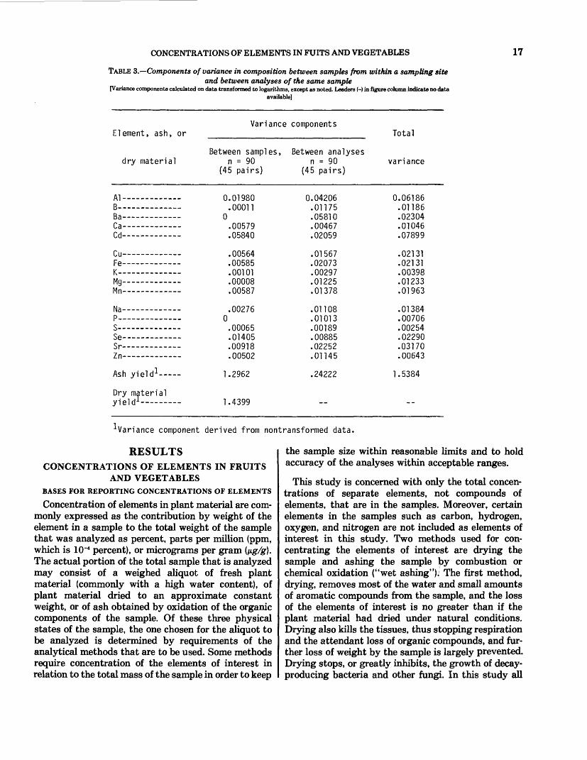
CONCENTRATIONS OF ELEMENTS IN FUITS AND VEGETABLES 17
TABLE 3.—Components of variance in composition between samples from within a sampling site and between analyses of the same sample
[Variance components calculated on data transformed to logarithms, except as noted. Leaders (-) in figure column indicate no dataavailable]
Element, ash, or
dry material
Variance components
Between samples,n = 90
(45 pairs)
Between analysesn = 90
(45 pairs)
Total
variance
B- Ba- Ca- Cd-
Cu- Fe- K- Mg- Mn-
0.01980.00011
0.00579
0.04206.01175.05810.00467
0.06186.01186
.01046
Na- P- S« Se- Sr- Zn-
0
Ash yield
Dry material yield 1 ———
.00564
.00585
.00101
.00008
.00587
.00276 ).00065 .01405 .00918 .00502
1.2962
1.4399
.01567
.02073
.00297
.01225
.01378
.01108
.01013
.00189
.00885
.02252
.01145
.24222
.02131
.02131
.00398
.01233
.01963
.01384
.00706
.00254
.02290
.03170
.00643
1.5384
Variance component derived from nontransformed data.
RESULTSCONCENTRATIONS OF ELEMENTS IN FRUITS
AND VEGETABLESBASES FOR REPORTING CONCENTRATIONS OF ELEMENTS
Concentration of elements in plant material are com monly expressed as the contribution by weight of the element in a sample to the total weight of the sample that was analyzed as percent, parts per million (ppm, which is 10~4 percent), or micrograms per gram (fig/g). The actual portion of the total sample that is analyzed may consist of a weighed aliquot of fresh plant material (commonly with a high water content), of plant material dried to an approximate constant weight, or of ash obtained by oxidation of the organic components of the sample. Of these three physical states of the sample, the one chosen for the aliquot to be analyzed is determined by requirements of the analytical methods that are to be used. Some methods require concentration of the elements of interest in relation to the total mass of the sample in order to keep
the sample size within reasonable limits and to hold accuracy of the analyses within acceptable ranges.
This study is concerned with only the total concen trations of separate elements, not compounds of elements, that are in the samples. Moreover, certain elements in the samples such as carbon, hydrogen, oxygen, and nitrogen are not included as elements of interest in this study. Two methods used for con centrating the elements of interest are drying the sample and ashing the sample ^>y combustion or chemical oxidation ("wet ashing"); The first method, drying, removes most of the water and small amounts of aromatic compounds from the sample, and the loss of the elements of interest is no greater than if the plant material had dried under natural conditions. Drying also kills the tissues, thus stopping respiration and the attendant loss of organic compounds, and fur ther loss of weight by the sample is largely prevented. Drying stops, or greatly inhibits, the growth of decay- producing bacteria and other fungi. In this study all
18 ELEMENTS IN FRUITS AND VEGETABLES, CONTERMINOUS UNITED STATES
plant samples were dried, after having determined their fresh weight, as soon as practical.
Ashing further concentrates most of the elements of interest by oxidizing organic compounds in the sam ple, thus removing much of the carbon, hydrogen, and some other elements from the sample. For analyzing the many elements that are relatively stable at com bustion temperatures, ash produced by burning is com monly used. Other elements such as arsenic, mercury, selenium, and sulfur are volatilized and lost from the sample at combustion temperatures; therefore, for their determination, samples are "ashed" by the use of strongly oxidizing reagents (hydrogen peroxide, per chloric acid).
Although the physical state of the material to be analyzed may be determined by requirements of par ticular analytical methods, the basis used for reporting element concentrations may be the weight percent (or parts per million) that the element constitutes of the fresh material, the dry material, or the ash if in the stages of sample preparation the weight lost by drying the sample and ashing the sample was recorded. Then the choice of the basis for reporting element concentra tions can be determined by the intended use of the data. If the data are expected to be used principally to evaluate dietary requirements or toxicities, either the fresh basis or the dry-weight basis is most appropriate. If the concentrations of elements are to be used for correlating plant and soil chemistry, values expressed on an ash-weight basis are commonly used.
For samples taken over a wide range of locations and physical conditions, data on element concentrations based on analysis of ash are more nearly stable (reproducible) than are those based on dry or fresh weight because two kinds of variation not directly related to the elements of interest, the water and the organic-matter contents, are eliminated. The fluctua tion in water content of a plant during a 24-hour period, from the wilted state to the fully turgid condi tion, can be very great. Likewise, but to a lesser extent, daily fluctuations in the amount of organic compounds in a plant or plant part may be appreciable owing to changes in relative rates of photosynthesis and respiration and to the movement of organic com pounds from one part of the plant to another part while the amounts of the elements of interest may remain relatively constant. Because the concentrations of elements are reported as proportions of total-sample aliquot weights, the weight fluctuations of the sample caused by loss of water and organic compounds may greatly affect the concentration of elements that is reported.
The parts of most plants (except the salad vegetables) used for human food are storage organs of
the plants such as seeds, fruits, stems, tubers, or roots. Whereas the elements obtained from the soil probably are largely deposited early in the formation of these organs and their amounts are only slowly increased during the maturation of these organs, the synthesis and deposition of sugars, fats, and starches increase rapidly toward the time of maturity of the storage organs. Therefore, if dried material is analyzed, the degree of maturity (ripeness, in fruits) of these tissues can greatly influence the reported concentrations of the soil-derived elements. If these dried samples are burned to ash, thereby eliminating the organic consti tuents, and the ash is analyzed, the effects of different degrees of maturity of the produce on the concentra tions of elements of interest are greatly reduced or removed. For these reasons it is important to specify the basis used for reporting element concentrations in plants and, particularly for food plants, the data re quired for conversion to other bases.
This report gives summaries of element concentra tions for each kind of fruit and vegetable on the basis of fresh weight, dry weight, and ash weight (except for the volatile elements), with the material used for analysis specified for each element as given in table 1. If the material actually analyzed was ash, the values obtained were converted to a dry weight basis using the following formula:
Md=(Mfl XMpa)/LOO, (3)
where Md approximates the mean in dry weight, Ma is the mean of the element in ash weight, and Mpa is the mean percent ash measured for the particular kind of fruit or vegetable.
If the material analyzed was dried fruits or vegetables and the analyst reported element concen trations on the dry-weight basis (in this study arsenic, mercury, selenium, and total sulfur were so reported), these values can be converted to approximate values in ash by using the following formula:
(4)Mpfl/ioo
where Ma approximates the mean in ash weight, is the mean of the element in dry material, and Mpa is the mean percent ash measured for the particular kind of fruit or vegetable.
The concentrations of elements reported on a dry- weight basis can be converted to approximate concen trations in fresh material by using the formula:
Mf=(MdXMpd)llQQ, (5)

CONCENTRATIONS OF ELEMENTS IN FRUITS AND VEGETABLES 19
where My approximates the mean in fresh material, is the mean of the element in dry material, and Mpd is the mean percent dry material in fresh material.
To convert concentrations of elements reported in ash to concentrations in fresh material, first convert ash-weight values to dry-weight values by using for mula 3 above; then convert the dry-weight values to fresh-weight values by using formula 5.
The mean percentage of water in the fresh fruits and vegetables can be calculated by subtracting the mean percent dry-material yield of fresh material (given in the last row of each table) from 100.
MEAN CONCENTRATIONS IN SAMPLES
The chemical composition of the ash of fruits and vegetables is first presented by grouping the data by areas of commercial production and giving the detec tion ratios, mean concentrations, deviations, and observed ranges for all elements studied for each kind of fruit or vegetable (tables 4-20). These data can be converted, if desired, to values based on dry material or fresh material by using formulas 3 and 5, respectively.
The analytical data for kinds of produce were sum marized by combining all county data into one matrix for a fruit or vegetable that was collected in more than one area of commercial production, and determining ratios, means, deviations, and ranges in element con centration for each kind of produce. The resulting means, deviations, and ranges were converted, as ap propriate, to three bases (fresh, dry, and ash weights) and are presented in tables 2 1 to 37. Data in these tables can be used as baseline values for these kinds of produce as grown in areas of commercial production in the United States.
Some kinds of fruits and vegetables were collected at a few sites in only one county, although they are widely grown commercially in this country. The data on these samples are given on fresh-, dry-, and ash—weight bases in tables 38 to 45. These data are not purported to represent the chemical characteristics of these fruits or vegetables as grown throughout this country in areas of commercial production but, nevertheless, sug gest general ranges in values that may be expected.
Some elements were determined infrequently in the plant samples and, therefore, were not entered in the tables of element concentrations. These elements, the fruit or vegetable in which found, the sampling localities, and the concentrations found, follow:
Gallium—Two samples of lettuce, CumberlandCounty, N.J., 10 and 15 ppm.
Lanthanum—One sample of plums, Berrien County,
Mich., 70 ppm; one sample of lettuce, CumberlandCounty, N.J., 70 ppm; and one sample of cabbage,Hidalgo County, Tex., 70 ppm.
Tin—One sample of grapefruit, Hidalgo County,Tex., 30 ppm.
Vanadium—One sample of pears, Berrien County,Mich., 15 ppm; nine samples of lettuce,Cumberland County, N.J., 17-70 ppm.
Ytterbium—Three samples of lettuce, CumberlandCounty, N.J., 2-3 ppm.
Yttrium—Three samples of lettuce, CumberlandCounty, N.J., 20-30 ppm.
Although looked for in the samples, the following elements, with their stated lower limits of deter mination in parts per million by multielement spec- trographic analysis, were not found: antimony, 300; beryllium, 4; bismuth, 20; cerium, 300; europium (looked for if lanthanum or cerium was found), 200; ger manium, 20; hafnium, 200; indium, 20; neodymium (looked for if lanthanum or cerium was found), 70; niobium, 20; palladium, 2; praseodymium (looked for if lanthanum or cerium was found), 200; rhenium, 70; samarium (looked for if yttrium value was greater than 50 ppm), 200; scandium, 5; tantalum, 500; tellurium, 5,000; thallium, 500; thorium, 500; tungsten, 300; and uranium, 1,000.
COMPOSITIONAL VARIATION AMONG AREAS, AMONG FIELDS WITHIN AREAS, AND WITHIN FIELDS
ANALYSIS OF VARIANCE
The variance components given in tables 46-62 reflect the amount and nature of the compositional variation within each type of produce. The total variance indicates the amount of variance present at all levels of the experimental design, including sample preparation and analysis. If the total variance is small, the concentration of the element in the specified type of produce tends to be uniform and somewhat indepen dent of its source, and the variance components may be of little or no interest. However, if the total variance is moderate or large, the variance components ex pressed as percentages of the total variance will serve to indicate the nature and origin of the variance pre sent and can be used as a basis for accumulating addi tional data more efficiently than would be possible otherwise. For example, if a large percentage of the total variance is between areas, there is a strong in dication that the accumulation of the element by the plant in question is environmentally controlled to some large extent. On the other hand, if a large percentage of the variance is at the lowest level, be tween sampling sites within fields, the indication is

20 ELEMENTS IN FRUITS AND VEGETABLES, CONTERMINOUS UNITED STATES
that most of the variance is erratic and caused by either very local environmental differences, laboratory procedures, chance, or a combination of these. The percentage variance at the lowest level can be taken as the maximum percentage of the variance in the data that can be ascribed to sample preparation and analysis, as pointed out in the previous section on statistical methods.
If further sampling is to be carried out for the purpose of estimating more precise compositional averages, the variance components can be used to design efficient sampling programs. For example, if little or no variance is present between areas, it is theoretically possible to obtain as good an average by taking all samples from one area as would be obtained by sampling many areas. If all the variance were at the lowest level, between sites within field, it would be efficient to collect all the samples from a single field. Caution would have to be exercised here, however, because the variance components tabulated in tables 46-62, like all variance components, are only estimates and are subject to errors that can be considerable. The components should be taken only as general indicators of the gross nature of compositional variability within each produce type.
SIGNIFICANT DIFFERENCES IN MEAN ELEMENTCONCENTRATIONS AMONG AREAS OF COMMERCIAL
PRODUCTION
The main purpose of the analysis-of-variance com putations which led to the results summarized in tables 46-62 was to identify compositional differences in produce grown in different areas. The differences found to be statistically significant are summarized in table 63. Individual means are from tables 4-37.
CONCENTRATIONS OF ELEMENTS AND pH OFSOILS THAT SUPPORTED THE FRUITS AND
VEGETABLES
In the tables of element concentrations and pH that follow, the geometric mean values and the ranges in values are given as parts per million for the minor elements and as percent for the major elements, based on the total weight of the sample aliquot (tables 64-99). No attempt was made to estimate the concen tration of the elements in soil that occurred in a form available to plants; the best measure of the availability of soil elements is the concentration of elements in the plant itself. The pH values are reported in standard units, using arithmetic means and standard devia tions.
COMPOSITIONAL VARIATION AMONG AREAS AND AMONG FIELDS WITHIN AREAS
ANALYSIS OF VARIANCE
Tables 100-116 give estimates of variance com ponents for the geochemistry of the soils between and within the same areas in which the produce was sam pled. The sampling design and analysis-of-variance model have been described in previous sections of this report.
The chemical compositions of the soil samples are given by grouping the data for the soils that supported each kind of fruit or vegetable in each area of commer cial production and giving the detection ratios, means, deviations, and observed ranges. By this grouping the chemical characteristics of soils from these areas can be readily compared. The extremes in concentration of an element provide an estimate of the ranges within which these crops are being profitably produced but, of course, do not necessarily define the maximum or minimum concentrations that each plant species can tolerate. The concentrations given represent the total concentrations of an element without consideration of the compounds in which the element occurs. This fact is emphasized in the data tables for carbon, iron, and sulfur, because analyses of these elements are often given separately for total amounts of organic or in organic compounds, or for different oxidation states of the elements. These data are given in tables 64-80.
Summaries of the analytical data for soils from all sampling areas were prepared by combining the data for each sampling area grouped according to the kind of fruit or vegetable plants that the soils supported. These summaries provide mean concentrations and ex tremes in ranges in soils for each kind of produce in major commercial production areas in the United States, as given in tables 81-97.
The summary statistics on the element concentra tions in soils that supported vegetable plants from only one area of commercial production are given in tables 98 and 99.
Some elements were determined infrequently in the soil samples, and, therefore, were not entered in the tables of element concentrations. These elements, the fruit or vegetable supported by the soil, the concentra tions found, and the sampling localities, follow: Cerium—One sample of apple soil, 200 ppm, Wayne
County, N.Y. One sample of potato soil, 700 ppm, and one sample of tomato soil, 150 ppm, Cumberland County, N.J. Two samples of asparagus soils, 150 and 200 ppm, Imperial Coun ty, Calif. Three samples of orange soils, 100, 150, and 200 ppm, Riverside County, Calif. One sample
TRENDS IN ELEMENT CONCENTRATIONS IN FRUITS AND VEGETABLES 21
of grapefruit soil, 150 ppm, Yuma County, Ariz. One sample of American grape soil, 100 ppm, Yakima County, Wash. One sample of dry bean soil, 150 ppm, Mesa County, Colo.
Molybdenum—One sample of orange soil, 10 ppm, Riverside County, Calif. One sample of snap bean soil, 2 ppm, Imperial County, Calif. One sample of snap bean soil, 2 ppm, and one sample of potato soil, 10 ppm, Twin Falls County, Idaho. One sam ple of potato soil, 50 ppm, Yakima County, Wash. One sample of dry bean soil, 3 ppm, Mesa County, Colo.
Neodymium—One sample of apple soil, 150 ppm, and one sample of snap bean soil, 70 ppm, Wayne County, N.Y. Five samples of potato soils, 50, 70, 70, 70, and 300 ppm, and one sample of tomato soil, 70 ppm, Cumberland County, N.J. Two samples of asparagus soils, 70 and 150 ppm, Im perial County, Calif. One sample of grapefruit soil, 70 ppm, and three samples of orange soils, 70, 70, and 100 ppm, Riverside County, Calif. One sample of American grape soil, 70 ppm, and one sample of European grape soil, 70 ppm, Yakima County, Wash. One sample of dry bean soil, 70 ppm, Mesa County, Colo.
Silver—One sample of American grape soil, 0.7 ppm, Berrien County, Mich. One sample of plum soil, 30 ppm, Wayne County, N.Y. One sample of tomato soil, 10 ppm, San Joaquin County, Calif.
SIGNIFICANT DIFFERENCES IN MEAN ELEMENTCONCENTRATION AND pH AMONG AREAS OF
COMMERCIAL PRODUCTION
These differences were compiled from the mean con centrations given by area in tables 64-80, and from the between-area significant variances given in tables 100-116. Mean concentrations of each element in all samples of soil that supported each kind of produce were obtained from tables 81-97. By examining these tables, the highest and lowest mean concentrations for areas were determined for each element and soil sup porting each kind of produce where significant dif ferences in element concentrations were found. From this examination, the areas having the extremes in ele ment concentrations in soils supporting the different fruit and vegetable plants were identified, and the results are given in table 117.
DISCUSSION OF RESULTS
TRENDS IN ELEMENT CONCENTRATIONS IN FRUITS AND VEGETABLES
Differences in the reported concentrations of an ele ment between kinds of produce or areas of production may be due to the relative abilities of the species to ab sorb the element in preference to other elements and to differences in the abundance and availability of the ele ment in the plant's environment.
The hydrogen and oxygen of water and the carbon of organic compounds are not elements of interest in this study, and their presence in the weighed aliquot of a sample that is analyzed affects the concentrations of other elements that are determined in the sample. The amounts of water and organic carbon in produce are subject to wide fluctuations, as was explained earlier; therefore, they were removed from the sample aliquots by drying and combustion to provide a more stable basis, concentrations in ash, for reporting concentra tions of most other elements in the sample. The more volatile elements that would be lost by combustion were determined by analyzing dry plant material, and concentrations of these elements are reported on a dry- weight basis. The differences in mean element concen trations that were found in this study reflect in some measure the element absorption capabilities of the plants as well as their geochemical environments.
AMONG KINDS OF PRODUCE
The trends in fruit and vegetable element concentra tions are discussed separately. The fruit samples con stitute a more homogeneous group than do the vegetable samples, because the kinds of tissue in fruits are less diverse than those of vegetable samples in that different plant organs, including roots, stems, leaves, fruits, and seeds, are included in the range of edible tissues in vegetables.
FRUITS
For convenience in distinguishing trends in the com position of fruits, the mean element compositions of the different kinds, and their percentages of water, were rearranged from tables 21-28 and are given in table 118. The means indicate clearly that certain elements vary widely in concentration among different kinds of fruits. The range in concentration is indicated by the computed high-to-low ratio for each element—the ratio of the highest mean concentration to the lowest.
Trends in the concentration of elements in these fruits, as shown by their high-to-low ratios, indicate characteristic element absorption or accumulation

22 ELEMENTS IN FRUITS AND VEGETABLES, CONTERMINOUS UNITED STATES
tendencies of the different fruit plants. The low ratios of the macronutrients potassium, phosphorus, magne sium, and sulfur may indicate a physiological control of absorption in response to metabolic requirements common to all the different fruits, or they may indicate the existence of a barrier in the translocation of the elements from the stems into the fruits. The low ratios may also be caused by a rather uniform concentration of these elements in the cultivated soils where the fruits are grown, where macronutrient fertilizers are commonly applied to the soils. The ratio of calcium, in contrast to the other macronutrients, is high, in dicating either a different genetically controlled response of the various fruit plants to calcium or, again, a difference in soils among the production areas.
The micronutrients boron, copper, iron, and zinc have low ratios (less than 3:1) similar to those of most macronutrients, but the ratio of manganese is some what higher (4.4:1). Although the ratio of, high-to-low values of molydbenum cannot be calculated, the means that are given indicate that it is very high.
The concentrations of the nonnutritive, nontoxic elements barium, cobalt, chromium, lithium, nickel, titanium, and zirconium tend to have somewhat greater ranges than do those of the nutritive elements, but aluminum has a low range and sodium and stron tium have very high ranges.
The nonnutritive elements generally considered to be toxic to plants (arsenic, cadmium, mercury, and lead) occur too erratically in measurable concentra tions for high-to-low ratios to be calculated, but a wide range in concentrations is shown by the available data. The concentrations of these elements are low in natural soils, but arsenic, mercury, and lead formerly were widely used as pesticides, and soils of many old or chards are contaminated with them. Cadmium in ab normal amounts in plants or soils may be suspected of resulting from pollution. With this group of elements, local variation in concentrations can be expected to occur. The range of selenium values is moderately wide, probably reflecting natural variation in soils among the sampling areas, but the levels of concentra tion do not suggest that plant toxicity will occur.
Some trends in mean element concentrations among species can be observed. Plums generally have low mean concentrations of the nutrient and nontoxic nonessential elements, and moderate to low values for the toxic elements. Peaches, which are closely related genetically to plums, do not show the same trends. Grapefruit and oranges are closely related species of the same genus and have quite similar mean concentra tions of most elements. Their mean lithium and sodium contents are noteworthy, but an examination of the concentrations by areas shows that this content is not
a genetic characteristic but rather an environmental ef fect. The two kinds of grapes show no close corre spondence in mean element concentrations, which may have resulted from the different methods of sample preparation used for the two species: seeds were removed from the European grape samples but were retained in the samples of American grapes. Apples and pears are closely related gentically, but exhibit little relationship in mean element concentrations. In summary, a genetic effect on element concentrations in fruits of closely related species was not conclusively demonstrated; the strongest evidence for this effect was provided by the similarities of concentrations in grapefruit and oranges.
VEGETABLES
For presenting trends in the composition of vegetables, the mean element contents of the different kinds, and their percentages of water, were rearranged from tables 29-37 and are given in table 119.
The macronutrients potassium, phosphorus, magne sium, and sulfur have relatively low ratios, with potas sium having the lowest range in concentrations (1.24:1). The macronutrient calcium has a high ratio. These trends are similar to those of fruits, although the ranges are somewhat wider, as might be expected because different organs of the vegetable plants were sampled. The ratios of the micronutrients copper, boron, iron, and zinc are also low. Molybdenum concen trations range from below the limit of determination to 84 ppm; the extremely high values occur in samples of snap beans and dry beans which, with other legumes, are known molybdenum accumulators.
The ranges in concentration of the nonnutritive non- toxic elements appear to exhibit no general pattern. Some element ratios that are extremely high are caused by very low estimates of the mean when the concentra tions were determined in only a few of the samples. For some of these elements, contamination of the sample by soil or by airborne pollutants is indicated. The con centrations of titanium, zirconium, and often aluminum and iron have been widely used to estimate contamination in plant materials, because these elements commonly are more concentrated in soil than in the ash of uncontaminated plant samples. This kind of contamination is indicated for snap beans that have high concentrations of these elements. The whole bean pod was used for the samples, and, although the pods were washed, it was difficult to remove all soil material from the pubescent, somewhat viscid, pods. In con trast to snap beans, samples of sweet corn had very low concentrations of these elements, which may be ex-

TRENDS IN ELEMENT CONCENTRATIONS IN FRUITS AND VEGETABLES 23
plained by the protection provided by the husks which envelop the grains.
Ratios for the toxic elements arsenic, cadmium, mer cury, and lead could not be calculated because some means were below the limit of determination, but ex amination of the means that were available shows a very wide range in concentrations. This wide range is attributed to airborne pollution, or contamination by pesticides, or both. Lead is a common airborne pollu tant; and lettuce, which has a large surface-to-volume ratio, has the highest lead concentration of any of the samples. Although the lettuce was washed, it is evi dent that much of the lead was not removed from the samples collected in one area. At this location the let tuce was a cultivar having heads that were more open than those of the cultivars sampled at the other loca tions. This difference in element content among cultivars probably was not caused by different root absorption characteristics but only by airborne con tamination that was not readily removable from the leaves.
The water content has a narrow range among the vegetables, except for dry beans. The measurements of water content were based on the weights of the samples soon after they were collected in the field, and, although the bean seeds appeared to be dry, they con tained about 15 percent water.
Well-known trends in element absorption among kinds of vegetables can be observed in the mean con centrations given in table 119. Cabbage is in a plant family (Cruciferae) that is characterized by the ready uptake of sulfur and selenium. Plants in the bean fam ily (Leguminosae) contain relatively large concentra tions of molybdenum. Sweet corn is known to absorb large concentrations of zinc, and potatoes contain somewhat elevated levels of potassium. Absorption characteristics of other kinds of vegetables are not as well known, or are unknown. Some apparent trends indicated in this table are worth noting. Cabbage ap pears to absorb significantly large concentrations of calcium, lithium, and sodium. The strontium content of carrots seems to be unusually high, as is barium in cucumbers. Both cultivars of beans have high iron values, in addition to molybdenum. Tomatoes are distinguished by having relatively low concentrations of all elements of this study.
AMONG AREAS OF COMMERCIAL PRODUCTION
The significant differences among areas for elements in each kind of fruit and vegetable given in the analysis-of-variance tables 46-62 were assigned to the counties having the highest and lowest concentrations, as determined from tables 4-20, and are grouped by
element and kind of produce in table 63. The counties having element concentrations in a fruit or vegetable that lie between the lowest and the highest concentra tions are not considered in this table, because their between-area significances were not tested.
Data in table 63 demonstrate that many significant differences exist in mean element concentrations among kinds of produce from the areas in which they were sampled. Area trends in element concentrations, however, cannot be readily deduced from this table because of differences in the concentration capabilities of the species for the different elements. If the data in this table are considered along with the element data for individual areas (tables 4-20) some general trends in element concentrations characteristic of certain elements and specific areas can be observed.
Large-scale trends are considered first, as distinguished for samples from the Eastern States (defined as those that lie east of the 97th meridian), and from the Western States (west of the 97th meridian).
Lithium. This element was found in only three samples of produce from the Eastern States, and these samples are suspected of being influenced by pollution, but it was found in some samples from each of the pro duction areas in the Western States. The citrus fruits illustrate this tendency. No lithium was found in samples of grapefruit and oranges from Florida, whereas the following mean concentrations (ppm in ash) were reported from the Western States: Hidalgo County, Texas, grapefruit 3.1, oranges 2.8; Riverside County, Calif., grapefruit 4.7, oranges 14; and Yuma County, Ariz., grapefruit 21, oranges 20.
Molybdenum. The concentrations of this element in produce have strong species and regional trends. All dry bean samples from all production areas contain measurable concentrations (mean ppm in ash) as follows: Wayne County, N.Y., 31; San Joaquin County, Calif., 67; Twin Falls County, Idaho, 103; and Mesa County, Colo., 180. In contrast, pears are not strong molybdenum concentrators, yet show marked dif ferences among areas as follows (mean ppm in ash): Berrien County, Mich., <7; Wayne County, N.Y., <7; Yakima County, Wash., <7; San Joaquin County, Calif., 1.4; and Mesa County, Colo., 7.3. Plums show a similar trend. This regional trend in molybdenum, with high values in Colorado, was found in all produce that was sampled in Mesa County.
Selenium. The trend in concentrations of this ele ment is very similar to that of molybdenum and may be illustrated by the mean concentrations (ppm in dry material) of oranges, as follows: Palm Beach County, Fla., <0.005; Hidalgo County, Texas, 0.0089; Yuma County, Ariz., 0.0075; and Riverside County, Calif., 0.020. This trend differs from that of molybdenum in
24 ELEMENTS IN FRUITS AND VEGETABLES, CONTERMINOUS UNITED STATES
that several kinds of produce have relatively high con centrations in New Jersey and lower concentrations in some Western States, as shown by the following exam ple of apples (mean ppm in dry material): Berrien Coun ty, Mich., below determination limit in all samples; Wayne County, N.Y., 0.0013; Gloucester County, N.J., 0.0040; Yakima County Wash., 0.0023; and Mesa County, Colo., 0.014. Selenium concentrations in all produce from Mesa County were higher by an order of magnitude than in the same produce from all other areas.
Sodium. Sodium concentrations range more widely among kinds of produce than among regions, but there is a definite trend in most produce toward higher con centrations in the Western States. This trend may be shown by lettuce as follows (mean ppm in ash): Cumberland County, N.J., 2,200; Palm Beach County, Fla., 5,500; Hidalgo County, Texas, 25,000; and Im perial County, Calif., 54,000.
Zinc. Regional trends in this micronutrient vary greatly among the kinds of produce. Some fruits have higher values in the Eastern States, as illustrated by apples (mean ppm in ash): Berrien County, Mich., 79; Wayne County, N.Y., 72; Gloucester County, N.J., 86; Yakima County, Wash., 49; and Mesa County, Colo., 50. Plums show the same regional trend, but other fruits do not. Sweet corn, a zinc accumulator, may have somewhat lower zinc values in the Western States, as suggested by the following analyses (mean ppm in ash): Berrien County, Mich., 1,200; Salem County, N.J., 920; Palm Beach County, Fla., 1,400; and Twin Falls County, Idaho, 590. Other vegetables do not show this trend.
The element concentrations in some samples of vegetables from the New Jersey counties suggest that the pollution, or contamination by agricultural prac tices, affects the amounts reported. Examples of unusually high values in produce from this area follow: Lettuce—arsenic, 1.3 ppm in dry material; chromium, 22 ppm in ash; lead, 11 ppm in ash; and titanium, 1,379 ppm in ash. Snap beans—arsenic, 0.037 ppm in dry material and mercury, 0.0057 ppm in dry material. Tomatoes—titanium, 11 ppm in ash. Moreover, the presence in vegetables from these counties of some elements that are only rarely reported in plants in dicates that pollution may be suspected as causative. The following elements, and their ppm in ash, were found only in lettuce from Cumberland County, N.J.: Gallium, two samples, 10 and 15 ppm; ytterbium, three samples, 2-3 ppm; and yttrium, three samples 20-30 ppm. One sample of lettuce contained 70 ppm lan thanum and nine samples contained 17-70 ppm vanadium—otherwise, lanthanum was found in only
one sample of plums and vanadium in one sample of pears, both from Michigan.
TRENDS IN ELEMENT CONCENTRATIONS IN SOILS SUPPORTING FRUITS AND VEGETABLES
AMONG KINDS OF PRODUCE
A comparison of the mean concentrations of elements in soils supporting each kind of produce is given in tables 120-121. The ratios of the highest values to the lowest values for each element in the soils are also given. By this means, the concentrations of an element characteristic of soils supporting the different kinds of produce can be compared, and the ratios can be used as a measure of ranges in the mean concentrations.
For fruits (table 120), soils supporting oranges are characterized by having far the greatest number of lowest element values, and European grape soils have the greatest number of highest values. General trends in soil-element characteristics are not apparent for the other kinds of produce.
In comparing the range of values for elements among soils supporting different kinds of fruits, arsenic and lead stand out as having extreme high-to- low ratios. The high concentrations for both elements occur in apple-orchard soils, and the low concentra tions for both were found in orange-grove soils. This fact suggests that these elements in soils originated principally from the use of insecticidal sprays and that some kinds of fruit trees were sprayed with lead arsenate more commonly than were other kinds. The high ratios of aluminum, iron, vanadium, and stron tium result from the low natural levels of these elements in the sandy soils of citrus groves contrasted with the high levels in soils of the West Coast grape districts. The high ratios for calcium and strontium in soils supporting vegetables probably reflect the re quirement of cabbage for basic soils high in calcium contrasted with the wide range in soil pH tolerated by sweet corn. The other ratios for produce are within low ranges for which the effects of natural soil chemistry, cultural requirements for specific crops, fertilizer prac tices, and contamination cannot be distinguished with the available data.
AMONG AREAS OF COMMERCIAL PRODUCTION
The areas having significantly different concentra tions of each element in soils supporting each kind of fruit and vegetable, as indicated by analysis of variance (tables 100-116), are listed in table 117. The extreme high and extreme low areas are given because the analysis of variance measures differences only be-

RELATIONSHIPS OF THE ELEMENT CONCENTRATIONS IN PLANTS AND THE CONCENTRATIONS IN SOILS 25
tween the extremes—the other areas fall somewhere between the two.
The most striking results shown in table 117 are the wide ranges in element and pH values that are tolerated by the different kinds of produce. Even the toxic elements in soils may have wide ranges in concen tration without preventing successful cultivation of the fruits and vegetables that were analyzed. For ex ample, soil supporting plums in Mesa County, Colo. contained a mean arsenic concentration of 37 ppm, while the soil in plum orchards in Yakima County, Wash, contained an average of 6.3 ppm. Potato-field soils in Twin Falls County, Idaho, averaged 1.1 ppm mercury, while those in Yakima County averaged only 0.032 ppm. Pear-orchard soils in Yakima County averaged 160 ppm lead, but those in Berrien County, Mich., averaged only 20 ppm. Even concentrations of the major nutrient elements calcium, potassium, and magnesium have order-of-magnitude differences in soils supporting a kind of produce. The latitude in pH values also may be wide; for example, both the acid soils of Wayne County, N.Y. (pH 4.8), and the alkaline soils of Twin Falls County, Idaho (pH 8.2), produce profitable crops of potatoes.
Some pronounced trends are shown among areas in mean element concentrations and pH in soils support ing the different kinds of produce. A large-scale trend is found in the high pH values of soils from the Western States and the lower values for those of the Eastern States that is related to similar differences in calcium and magnesium concentrations in the cultivated zone of soils. Similar trends are shown by lithium and sodium.
Less distinct differences in east-to-west soil concen trations, but for which the Western States generally have higher element values, are shown by aluminum, barium, cobalt, chromium, iron, gallium, germanium, nickel, rubidium, scandium, strontium, thorium, titanium, uranium, vanadium, yttrium, ytterbium, and zinc. Locations sampled in the Eastern States tend to have higher concentrations only of silicon, which is probably caused by leaching of soil elements that are more mobile than silicon.
No clear regional trends are shown in concentrations of arsenic, boron, carbon, copper, fluorine, mercury, potassium, manganese, lead, and tin. If regional dif ferences in concentration of these elements in soils originally existed, they have been diminished or obliterated by cultivation practices or contamination. Boron, copper, manganese, and potassium are defi cient for profitable growth of fruits and vegetables in some areas and may be added to the soil in fertilizers. Total carbon concentration in soil is influenced by the content of organic matter and carbonates in soils
which may range widely within areas and so obscure regional patterns. Arsenic, mercury, copper, and lead were formerly used as pesticides throughout the United States, and residues of these elements persist in some soils. The remaining elements fluorine and tin, as well as arsenic, mercury, and lead, may be added to the soil by industrial or vehicular pollution.
Reasons for the differences in element concentra tions in soils that support different kinds of produce within an area are not obtainable from the tables given in this report; they can be deduced only from observa tions made at the different sites. For example, soils supporting lettuce in Florida and potatoes in New York are much higher in carbon than are the soils in which some other crops are grown in the areas because in these two States lettuce and tomatoes were grown in peat or muck while the other kinds of produce were grown in less organic soils. The high lead and arsenic levels in soils at apple-orchard sites in both Washington and Michigan relate to spray residues in old orchards, whereas soils of young orchards have lower concentrations of these elements. Soils of the sampling area in Cumberland County, N.J. probably reflect effects of contamination, as indicated by the un common soil elements found and the concentrations of other elements that are often associated with local pollution.
The effects of fertilization within and among areas cannot be evaluated from the data at hand, but as a general practice labor-intensive crops, including most kinds of fruits and vegetables, are heavily fertilized with the major nutritive elements. These fertilizers may contain trace amounts of undesirable elements such as cadmium in phosphates that can remain in the plow zone of soils for long periods of time. Certain micronutrient elements, such as copper, zinc, boron, and manganese, may be applied to the soil in areas having deficiencies of these elements. Large quantities of sewage sludge or other organic wastes were ob served in vegetable fields in Imperial County, Calif., and these materials probably were also used in other areas. These wastes often contain significant amounts of undesirable heavy metals.
RELATIONSHIPS OF THE ELEMENT CONCEN TRATIONS IN FRUITS AND VEGETABLES AND
THE CONCENTRATIONS IN SOILS
Numerous studies have demonstrated that the con centration of an element in plant tissue commonly has only little correlation with the total concentration of the same element in the soil that supported the plant. This lack of correlation is caused by the fact that only certain chemical states of an element can be absorbed

26 ELEMENTS IN FRUITS AND VEGETABLES, CONTERMINOUS UNITED STATES
by plants; another reason is that inherent physio logical characteristics of plant species control the con centrations that can be absorbed. There is no universal laboratory method of determining the availability of the elements in soils to plants; therefore, this study considered only total element concentrations, not available concentrations.
If the concentrations of an element in soils exceed certain concentrations that can be considered "normal," the plants may reflect the high soil levels by their increased absorption of the element. This reac tion forms the basis for biogeochemical prospecting for mineral deposits. Agricultural soils have element con centrations that range within the requirements or tolerances of the cultivated plants; therefore, ex tremely high concentrations of toxic elements, or extremely low concentrations of nutritive elements, are not expected in these soils. Contamination or pollu tion, however, may cause local high concentrations of certain elements in agricultural soils. Moreover, natural differences in concentrations on a continental scale may be of sufficient magnitude for some elements in soils to elicit a corresponding response in plant ele ment concentrations.
An examination of the tables giving mean element values for fruits and vegetables by areas of production (tables 4-21) and corresponding tables for soils in which these plants grew (tables 64-80) reveal some large-scale examples of plant element-soil element cor relations. The following examples of correlation are
Sample No.
01AP110S01AP120S
SoilAs
9013
(ppm)Pb
20070
Sample No.
01 API 10001AP1200
FruitAs1
810
(ppm)Pb2
1,0001,500
Very few correlations of the kinds given above are evident in the data on mean element concentrations in produce and soils. Doubtless, the averaging of concen trations for areas has obscured some of the correla tions that exist at the site level.
The plant-soil relationships at some sampling sites showed a strong influence of soil element concentra tions on the abundance of some elements in the plants. Analyses of plants and soils at each sampling site are not given in this report, but were published by Boern- gen and Shacklette (1980). The following relationships of soil and plant element contents are based on site data from the latter report.
Some sites in old apple orchards in Michigan showed the influence of having been sprayed with arsenate of lead over a period of many years, as follows (paired soil-fruit samples):
'in dry material. 2In ash.
A second example follows, in which samples were collected from an old apple orchard in Washington said by the owner to be about 30 years old and to have been sprayed with arsenate of lead four to five times per year for many years.
ueneveu tu reiate tu natural sun unierences in elementconcentrations:
Area Soil Fruit
Mean lithium concentrations (ppm) in ash of grapefruit and in associated soils
Florida ................................. 0.54Texas .................................. 14California ............................... 28Arizona ................................ 27
<43.1 4.7
12
Mean lithium concentrations (ppm) in ash of oranges and in associated soils
Florida ................................. 6.3Texas .................................. 15
<4 2.8
14 20
Mean sodium concentrations (ppm) in ash of American grapes and in nssociated soils
Michigan ............................... 1,200New York .............................. 11,000Washington ............................ 17,000
220 230
1,200
Mean potassium concentrations (ppm) in ash of European grapes and in associated soils
California ............................... 2.014 29
Soil (ppm) Fruit (ppm) Sample No. As Pb Sample No. As1 Pb2
09AP410S 114 700 09AP4100 0.3 <10 09AP510S 135 1,000 09AP5100 0.3 <10
'In dry material. 2In ash.
In both examples, the soils contained unusually high concentrations of arsenic and lead, if compared to "typical" soil concentrations, but the response of the apple trees, as measured by the content of these elements in the fruits, was not consistent. The apple samples from Michigan indicated positive, but not pro portional, responses to soil concentrations, whereas the apple samples from Washington exhibited no response to even higher soil concentrations of these elements. These erratic responses probably did not reflect surface contamination of the fruits, because all apple samples were pared, and the peel was discarded. The apple trees in Washington were irrigated, whereas those in Michigan depended entirely upon rain and snow for their supply of water. It is not clear how this difference in water supply could affect the availability of the two elements to the trees.
SUMMARY 27
Analyses of paired soil-plant samples for arsenic from an area in Cumberland County, N. J., thought to be af fected by pollution follow:
Sample No.
03LH210S03LH110S03LH510S03LH310S03LH410S
SoU (ppm)
4.711.712.613.017.9
Sample No.
03LH210003LH110003LH510003LH310003LH4100
Lettuce1 (ppm)
1.01.52.02.57.0
'in dry material.
These high arsenic levels in both soil and lettuce are most likely caused by air or soil pollution, or both, but not by contamination with arsenate of lead insecticide, because the lead values for the soils in this area are within the normal range. The abnormally high ash values found in these plant samples indicate con tamination by soil that was not removed when the let tuce was washed.
Copper values for potato tubers and soils from the New Jersey sites are anomalously high. However, the high values in the potato samples were not caused by soil contamination of the samples, as may have occur red with the lettuce samples, because the potatoes were peeled and the peels were discarded. Mean copper values for potatoes and potato-field soils from all areas follow.
Area
Idaho ....................
Soil 1 (ppm)
........... 17
........... 20
........... 40
........... 140
Potato (ppm in ash)
627498
135
The high copper values for New Jersey soils and potatoes strongly suggest effects of soil pollution.
The highest and lowest mean element concentrations that are significantly different in produce and soils among areas of commercial production are given by county in tables 63 and 117. The mean concentrations for each kind of produce and its supporting soils are also given. These tables serve as a ready reference for locating strong regional trends in element concentra tions; they also delineate the predominant trends in soil element-plant element relationships. Only the areas having extreme values for each category of samples are given, as indicated by analysis-of-variance procedures. Other values by area for soils and produce fall somewhere between the extremes and can be found in summary tables given elsewhere in this report.
Striking features presented in tables 63 and 117 are the large numbers of significant differences that are identified and, for many elements, the magnitude of the differences. Another feature that is evident is the general lack of correspondence of extreme values be tween soils and produce. Very few examples can be found for which a county has the extreme values for an element in both soils and the produce grown on the same group of soils. This fact supports the general principle that ordinarily there is a low degree of cor relation between the total concentration of an element in soils and the concentration in an associated species of plant. Only when soil element concentrations exceed a certain level do plants respond with a corresponding increase in content of that element. This level of response differs widely among elements and plant species and is also influenced by many external environmental factors. These complex relationships cannot be generalized quantitatively, but must be determined on a case-by-case basis. For this reason the generally accepted principle is that the best measure of soil element availability is the amount found in the plant itself.
SUMMARY
Estimates of the mean concentrations of 27 chemical elements in eight kinds of fruits and nine kinds of vegetables, based on field collections of produce from 11 areas of commercial production in the United States, provided data that can be used as background values for these elements in produce before their con centrations have been altered by harvesting, process ing, or cooking. The water content of the samples was determined in the field and the ash yield of all dried samples was recorded; these measurements permitted the mean concentrations to be expressed on a fresh, dry, or ash basis.
The sampling design that was followed required the sampling of produce in 11 areas, in five fields in each area, and at two sites in each field. In addition, a duplicate sample of produce was collected at 45 sites that were randomly selected before sampling was begun. This procedure permitted the use of analysis of variance techniques to determine the distribution of variation in element concentrations among areas of production, among fields within areas, and between sites within fields.
Most variation in element concentrations was among areas. Variation at the site level included errors in sampling, preparation, and analysis, in addition to the natural variation that was influenced by factors of the environment at the site. The data from the 45 duplicate field collections and from 45 randomly selected laboratory sample splits were used to
28 ELEMENTS IN FRUITS AND VEGETABLES, CONTERMINOUS UNITED STATES
estimate separately the effects of these factors. As a general rule, the sampling and analytical errors were judged to be within acceptable limits.
A test to determine the differences in concentrations of elements at the 0.05 probability level among areas of fruit and vegetable production revealed many signifi cant differences in the extreme mean concentrations of elements among the different kinds of produce. The causes of these differences that could be determined with reasonable confidence were distributed on a case by case basis among natural soil differences, culti vation practices, contamination by pesticides, and pollution.
The cultivated zone of soils was sampled at each site where produce was sampled, except where duplicate field and site samples of produce were collected. Analysis of variance revealed many more significant differences in concentrations of elements in soils at the area level than were found in produce. Only the total concentrations of each element were determined in the soil samples—no attempt was made to define available concentrations by laboratory procedures, because the actual amount absorbed by the plant is the best measure of availability of elements in soils.
Correlations between the total concentration of an element in soil and in produce samples were generally absent or low. A few positive correlations at an area scale were attributed to differences in the natural con centrations of an element in the soil, but others most probably resulted from contamination or pollution ef fects on the soil or the produce.
Trends in element concentrations among kinds of produce identified the fruits and vegetables which con centrated certain elements in their tissues relative to concentrations in others and indicated either a strong species control, or an environmental control related to areas of production, or both. The trends in element con centrations in soils generally showed a pronounced geographical control, to which, at places, contamina tion and pollution effects were added.
CONCLUSIONS
1. The concentrations of elements in fruits and vegetables generally differ least in the macronutrients potassium, phosphorus, magne sium, and sulfur that are essential for plant growth. Trends in concentrations of the micro- nutrients boron, copper, iron, and zinc are similar but not as pronounced as those of the macro- nutrients. The concentrations of the nonnutritive, nontoxic elements barium, cobalt, lithium, nickel, titanium, and zirconium tend to have greater ranges than do those of the nutritive elements.
Concentrations of elements generally considered toxic to organisms exhibit erratic distributions among areas and kinds of produce, and a wide range in their concentrations is indicated.
2. The total amounts of most elements in soils have only little effect on the amounts in the produce as long as concentrations are at the levels found in soils of areas where fruits and vegetables are com mercially produced. If soil levels exceed these ill- defined or unknown levels, either from natural causes or from contamination or pollution, concen trations in produce may reflect these excessive levels in soils.
3. Regional differences in concentrations as great as tenfold were found for some elements in various kinds of produce. These trends may be useful in examining epidemiological peculiarities; dietary recommendations may also be influenced by these differences. Caution should be used, however, in applying grand mean concentrations of elements in produce to specific environmental or nutritional problems.
4. The concentrations of various elements in the produce sampled in this study, whether due to normal soil levels or to contamination or pollution, represent levels that may be found in fruits and vegetables in commercial markets insofar as the sampling adequately covered the major areas of production. These levels may be reduced or in creased by various methods of food processing and preparation. The significance of the concen trations as applied to problems of nutrition and health of humans or animals is left to the judg ment of investigators in the medical sciences.
REFERENCES CITEDAllaway, W. H., 1968, Agronomic controls over the environmental
cycling of trace elements: Advances in Agronomy, v. 20, p. 235-274.
Beeson, K. C., 1941, The mineral composition of crops with par ticular reference to the soils in which they were grown—A review and compilation: U.S. Department of Agriculture Miscellaneous Publication 369,164 p.
___1957, Soil management and crop quality, in U.S. Department of Agriculture, Soil—Yearbook of Agriculture 1957: U.S. Government Printing Office, p. 258-267.
Bennett, C. A., and Franklin, N. L., 1954, Statistical analysis in chemistry and the chemical industry: New York and London, John Wiley & Sons, Inc., 724 p.
Boerngen, J. G., and Shacklette, H. T., 1980, Chemical analysis of fruits, vegetables, and their associated soils from areas of com mercial production in the conterminous United States: U.S. Geological Survey Open-File Report 80-84,134 p.
Chapman, H. D., ed., 1966, Diagnostic criteria for plants and soils: Riverside, Calif., University of California, Division of Agricultural Science, 793 p.

REFERENCES CITED 29
Cohen, A. C., Jr., 1959, Simplified estimators for the normal distribution when samples are singly censored or truncated: Technometrics, v. 1, no. 3, p. 217-237.
Connor, J. J., and Shacklette, H. T, 1975, Background geochemistry of some rocks, soils, plants, and vegetables in the conterminous United States, with sections on Field studies by R. J. Ebens, J. A. Erdman, A. T. Miesch, R. R. Tidball, and H. A. Tourtelot: U.S. Geolological Survey Professional Paper 574-F, 168 p.
Diem, Konrad, ed., 1962, Scientific tables, 6th ed.: Ardsley, New York, Geigy Pharmaceuticals, Division of Geigy Chemical Corp., 778 p.
Duke, J. A., 1970, Ethnobotanical observations on the Choco In dians: Economic Botany, v. 24, no. 3, p. 344-366.
Egan, Harold, 1972, Trace lead in food, in Hepple, Peter, ed., Lead in the environment: London, Institute of Petroleum, p. 34 42.
Garber, K., 1968, Uber den Fluorgehalt von Pflanzen, in Deutsche Forschungsgemeinschaft, Fluor-Wirkungen—Forschung- sergebnisse bei Pflanze und Tier, Forschungsberichte 14, [The fluorine content of plants, in German Research Society, Effects of fluorine—Results of research with plants and animals, Research report 14]: Wiesbaden, Franz Steiner Verlag, p. 42-48.
Goodall, D. W., and Gregory, F. G., 1947, Chemical composition of plants as an index of their nutritional status: Imperial Bureau of Horticulture and Plantation Crops, East Mailing, Kent, England, Technical Communication 17,167 p.
Gough, L. P., and Shacklette, H. T., 1979, Element concentrations toxic to plants, animals, and man: U.S. Geological Survey Bulletin 1466,80 p.
Harms, T. F., 1976, Analysis of plants and plant ashes by methods other than emission spectroscopy, in Miesch, A. T., Geochemical survey of Missouri—Methods of sampling, laboratory analysis, and statistical reduction of data: U.S. Geological Survey Professional Paper 954-A, p. 17-18.
Huffman, Claude, Jr., and Dinnin, J. I., 1976, Analysis of rocks and soils by atomic absorption spectrometry and other methods, in Miesch, A. T., Geochemical survey of Missouri—Methods of sampling, laboratory analysis, and statistical reduction of data: U.S. Geological Survey Professional Paper 954-A, p. 12-14.
Imperial County Board of Supervisors, 1971, Imperial County Agriculture, 1971: [Sacramento, California] Office of the Agricultural Commissioner, 6 p.
Kenworthy, A. L., 1967, Plant analysis and interpretation of analysis for horticulture crops, in Plant analysis, pt. 2 o/Stelly, Matthias, ed., Soil testing and plant analysis: Madison, Wise., Soil Science Society of America Special Publication Series 2, p. 59-75.
Kropf, R., and Geldmacher-v.Mallinckrodt, M., 1968, Der Cad- miungehalt von Nahrungsmitteln und die tagliche Cadmium- aufnahme [The cadmium content of foodstuffs and the daily cadmium intake]: Archiv flir Hygiene, v. 152, no. 3, p. 218-224.
Miesch, A. T., 1967, Theory of error in geochemical data: U.S. Geological Survey Professional Paper 574-A, 17 p.
___1976, Geochemical survey of Missouri—Methods of sam pling, laboratory analysis, and statistical reduction of data: U.S. Geological Survey Professional Paper 954-A, 39 p.
Millard, H. T., Jr., 1975, Determinations of uranium and thorium in rocks and soils by the delayed neutron technique, in U.S. Geological Survey, Geochemical Survey of the western coal regions, Second Annual Progress Report, July 1975: U.S. Geological Survey Open-File Report 75-436, p. 79-81.
Miller, Judith, 1974, Agriculture—FDA seeks to regulate genetic manipulation of food crops: Science, v. 185, no. 4147, p. 240-242.
Monier-Williams, G. W., 1949, Trace elements in food: London, Chapman & Hall, Ltd., 511 p.
Morrison, G. H., Pierce, J. O., Allaway, W. H., Angino, E. E., Cannon, H. L., Jorden, Roger, Kubota, Joe, Laitinen, H. A., and Lakin, H. W., 1974, Sampling, sample preparation, and storage for analysis, chap. 11 in The relation of selected trace elements to health and disease, v. 1 of Geochemistry and the environ ment: Washington, D.C., National Academy of Science, p. 90-97.
Neiman, H. G., 1976, Analysis of rocks, soils, and plant ashes by emission spectroscopy, in Miesch, A. T., Geochemical survey of Missouri—Methods of sampling, laboratory analysis, and statistical reduction of data: U.S. Geological Survey Profes sional Paper 954- A, p. 14-15.
Pickersgill, Barbara, 1977, Taxonomy and the origin and evolution of cultivated plants in the New World: Nature, v. 268, 18 August 1977, p. 591-595.
Quarterman, John, 1973, Factors which influence the amount and availability of trace elements in human food plants: Plant Foods and Human Nutrition, v. 23, no. 1/3, p. 171-190.
Shacklette, H. T., 1972, Cadmium in plants: U.S. Geological Survey Bulletin 1314-G, 28 p.
Shacklette, H. T., Erdman, J. A., Harms, T. F., and Papp, C. S. E., 1978, Trace elements in plant foodstuffs, chap. 3 in pt. 1, Oehme, F. W., ed., Toxicity of heavy metals in the environment, of vol. 2, Hazardous and toxic substances: New York, Marcel Dekker, Inc., p. 25-68.
Shacklette, H. T., Sauer, H. I., and Miesch, A. T., 1970, Geochemical environments and cardiovascular mortality rates in Georgia: U.S. Geological Survey Professional Paper 574-C, 39 p.
Stipe, G. J., and Jones, K. W., comp., 1972, Agricultural report: [Stockton, Calif.] San Joaquin County Department of Agriculture, 20 p.
Underwood, E. J., 1971, Trace elements in human and animal nutri tion (3d ed.): New York and London, Academic Press, 543 p.
___1973, Trace elements, chap. 3 in Toxicants occurring natu rally in foods (2d ed.): Washington, D.C., National Academy of Sciences, p. 43-87.
U.S. Food and Drug Administration, 1972, General pro gram—Foods, chap. 20 in Compliance program guidance manual: Washington, D.C., U.S. Food and Drug Administra tion, 16 p. plus Attachments A, B1-B4, C, D.
U.S. Geological Survey, 1970, The national atlas of the United States of America: Washington, D.C., U.S. Department of the Interior, 417 p.
U.S. Soil Conservation Service, 1969, Distribution of principal kinds of soils—Orders, Suborders, and Great Groups, in The national atlas of the United States of America: U.S. Geological Survey, sheet 86,2 p.
Vernon, R. O., and Puri, H. S., 1964, Geologic map of Florida: U.S. Geological Survey, and Florida Board of Conservation, Division of Geology, Map Series 18,1 sheet.
Wahlberg, J. S., 1976, Analysis of rocks and soils by X-ray fluorescence, in Miesch, A. T., Geochemical survey of Missouri—Methods of sampling, laboratory analysis, and statistical reduction of data: U.S. Geological Survey Profes sional Paper 594-A, p. 11 lr 12.
Warren, H. V., 1967, Lead in potatoes: Royal College of General Practioners Journal, v. 25, p. 66-72.
Washington State Department of Agriculture, 1964, Yakima County Agriculture: Olympia, County Agriculture Data Series 1964,69 p.

30 ELEMENTS IN FRUITS AND VEGETABLES, CONTERMINOUS UNITED STATES
Watt, B. K., and Merrill, A. L., 1950, Composition of foods—Raw, processed, prepared: U.S. Department of Agriculture, Agriculture Handbook 8,147 p.
Williams, K. T., and Whetstone, R. R., 1940, Arsenic distribution in soils and its presence in certain plants: U.S. Department of Agriculture Technical Bulletin 732,20 p.

TABLES 4-121

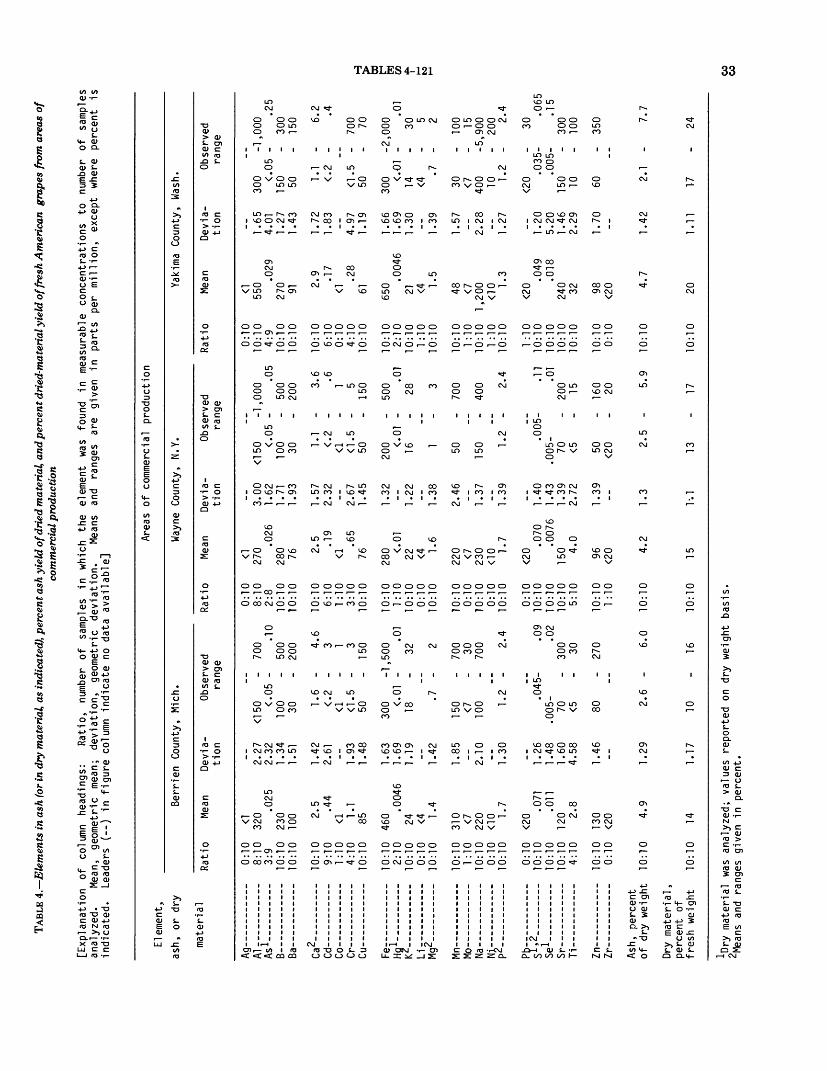
TABL
E 4.—
Ele
men
ts in
ash
(or i
n dr
y m
ater
ial,
as in
dica
ted)
, per
cent
ash
yie
ld o
f dri
ed m
ater
ial,
and p
erce
nt d
ried-
mat
eria
l yie
ld o
f fre
sh A
mer
ican
gra
pes
from
are
as o
fco
mm
erci
al p
rodu
ctio
n
[Exp
lana
tion
of
colu
mn
head
ings
: R
atio
, nu
mbe
r of
sa
mpl
es
in
whi
ch
the
elem
ent
was
foun
d in
m
easu
rabl
e co
ncen
trat
ions
to
nu
mbe
r of
sa
mpl
es
anal
yzed
. M
ean,
ge
omet
ric
mea
n;
devi
atio
n,
geom
etric
de
viat
ion.
M
eans
an
d ra
nges
ar
e gi
ven
in
part
s pe
r m
illio
n,
exce
pt
whe
re
perc
ent
is
indi
cate
d.
Lead
ers
(--)
in
fig
ure
col
umn
indi
cate
no
data
ava
ilab
le]
Elem
ent,
ash,
or
dry
mat
eria
l
An
--A
l _ _
_ _
_ _
_ttl
T —
— --------
Acl
Ra_
_
Ca2-
f\ j Co
——
- ——
o _
_ _
_ -
Cu —
- —
——
—
Fe —
——
——
——
Hnl
Hg
——
——
——
——
i/Z Li —
- —
—M
g^ —
— -
——
—
Mn —
——
——
——
Mo —
——
——
——
Ma
_
Ni—
— --
---
pZ —
— —
— —
—
Pb-- —
——
—Sl
»2__
____
___
L1—
— —
-S
r- _
-- _
-- _
Ti _
__
___
_ _
Zn —
——
——
——
7w»
Ash,
pe
rcen
t of
dry
wei
ght
Dry
mat
eria
l ,
perc
ent
of
fres
h w
eigh
t
*Dry
mat
eria
l
Area
s of
com
mer
cial
pr
oduc
tion
Ber
rien
Cou
nty,
M
ich.
Rat
io
Mean
D
evia
tio
n
0:10
<1
8:
10
320
3:9
10:1
0 23
0 10
:10
100
10:1
0 2.
9:
10
1:10
<1
4:
10
1.
10:1
0 85
10:1
0 46
0 2:
10
10:1
0 24
0:
10
<4
10:1
0 1.
10:1
0 31
0 1:
10
<7
10:1
0 22
0 0:
10
<10
10:1
0 1.
0:10
<2
0 10
:10
10:1
0 10
:10
120
4:10
2.
10:1
0 13
0 0:
10
<20
10:1
0 4.
10:1
0 14
was
anal
yzed
2.27
02
5 2.
32
1.34
1.
51
5 1.
42
44
2.61
1 1.
93
1.48
1.63
00
46
1.69
1.
19
4 1.
42
1.85
2.10
7 1.
30
071
1.26
O
il 1.
48
1.60
8
4.58
1.46
9 1.
29
1.17
Obs
erve
d ra
nge
<150
-
700
<.05
-
.10
100
- 50
0 30
-
200
1.6
- 4.
6 <.
2 -
3 <1
-
1 <1
.5
- 3
50
- 15
0
300
-1,5
00
<.01
-
.01
18
- 32
.7
- 2
150
- 70
0 <7
-
30
100
- 70
0
1.2
- 2.
4
.045
- .0
9 .0
05-
.02
70
- 30
0 <5
-
30
80
- 27
0
2.6
- 6.
0
10
- 16
; va
lues
re
po
rte
don
dry
wei
ght
Rat
io
0:10
8:
10
2:8
10:1
0 10
:10
10:1
0 6:
10
1:10
3:
10
10:1
0
10:1
0 1:
10
10:1
0 0:
10
10:1
0
10:1
0 0:
10
10:1
0 0:
10
10:1
0
0:10
10
:10
10:1
0 10
:10
5:10
10:1
0 1:
10
10:1
0
10:1
0
basi
s.
Way
ne C
ount
y
Mea
n
<1
270 .0
26
280 76 2.
5 .19
<1 .6
5 76 280 <.
01
22
<4 1.6
220 <7
230
<10 1.
7
<20
.070
.0
076
150 4.
0
96
<20 4.
2
15
Dev
ia
tio
n
3.00
1.
62
1.71
1.
93
1.57
2.
32
2.67
1.
45
1.32
1.22
1.38
2.46
1.37
1.39
1.40
1.
43
1.39
2.
72
1.39
1.3
l-.l
, N
.Y• O
bser
ved
rang
e
<150
-1
,00
0
<.05
-
.05
100
- 50
0 30
-
200
1.1
- 3.
6 <.
2 -
.6
<1
- 1
<1.5
-
5 50
-
150
200
- 50
0 <.
01
- .0
1 16
-
28
1 -
3
50
- 70
0
150
- 40
0
1.2
- 2.
4
.00
5-
.11
.005
- .0
1 70
-
200
<5
- 15
50
- 16
0 <2
0 -
20
2.5
- 5.
9
13
- 17
Rat
io
0:10
10
:10
4:9
10:1
0 10
:10
10:1
0 6:
10
0:10
4:
10
10:1
0
10:1
0 2:
10
10:1
0 1:
10
10:1
0
10:1
0 1:
10
10:1
0 1:
10
10:1
0
1:10
10
:10
10:1
0 10
:10
10:1
0
10:1
0 0:
10
10:1
0
10:1
0
Yakim
a
Mean
<1
550 .0
29
270 91 2.
9 .17
<1 .2
8 61 650
.004
6 21
<4
1.5
48
<7
1,20
0 <1
0 1.3
<20
.049
.0
18
240 32 98
<2
0 4.7
20
Cou
nty,
W
ash
Dev
ia
tion
1.65
30
0 4.
01
< 1.
27
150
1.43
50
1.72
1
1.83
<
4.97
<1
1.
19
50
1.66
30
0 1.
69
< 1.
30
14
<4
1.39
1.57
30
<7
2.
28
400 10
1.
27
1
<20
1.20
5.
20
1.46
15
0 2.
29
10
1.70
60
1.42
2
1.11
T7
• Obs
erve
d ra
nge
-1,0
00
.0
5 -
.25
- 30
0 -
150
.1
- 6.
2 .2
-
.4
.5
- 70
0 -
70
-2,0
00
.€
1 -
.01
- 30
5 .7
-
2
- 10
0 -
15
-5,9
00
-
200
.2
- 2.
4
- 30
.0
35
- .0
65
.005
- .1
5 -
300
- 10
0
- 35
0
.1
- 7.
7
- 24
1 E CO
if*. t->
to t-> CO
CO

CO
TABL
E 5,
—El
emen
ts in
ash
(or i
n dr
y m
ater
ial,
as in
dica
ted)
, per
cent
ash
yie
ld o
f dri
ed m
ater
ial,
and
perc
ent d
ried
-mat
eria
l yie
ld o
f fre
sh a
pple
s fr
om a
reas
of c
omm
erci
alpro
duct
ion
[Exp
lana
tions
of
colu
mn
head
ings
: R
atio
, nu
mbe
r o
f sa
mpl
es
in w
hich
the
el
emen
t wa
s fo
und
imm
easu
rabl
e co
ncen
trat
ions
to
r in
dic
ate
d.
Mea
n,
geom
etric
mea
n.
Dev
iatio
n,
geom
etric
de
via
tion
. Le
ader
s (-
-)
in fig
ure
col
umn
indic
ate
no
dat
a ava
ilable
]
Ele
men
t, as
h,
or
dry
mat
eria
l
Ag~
— —
—m
-- —
— --
.'
Caz_
_
Fer
— ---
---
H?l..........
u ..
....
....
si.z—
... —
Sel- —
— ... ..
.
Ash,
pe
rcen
t of
dry
wei
ght
Dry
mat
eria
l ,
perc
ent
of
fre
sh w
eigh
t
Ory
m
ater
ial
Ber
n' e
n C
ount
y
Rat
io
Mea
n
0:10
<1
9:
10
460
8:10
.4
5 10
:10
410
10:1
0 77
10:1
0 .8
7 7:
10
.18
0:10
<1
8:
10
.50
10:1
0 62
10:1
0 40
0 8:
10
.022
10
:10
29
0:10
<4
10
:10
1.3
10:1
0 84
2:
10
4.3
10:1
0 35
0 1:
10
<10
10:1
0 2.
2
3:10
54
10
:10
.025
0:
10
<.00
5 10
:10
46
9:10
16
10:1
0 79
0:
10
<20
10:1
0 1.
6
10:1
0 16
Dev
ia
tion
2.83
1.
48
1.30
1.
92
1.37
1.
50
3.00
1.
38
1.52
3.
12
1.33
1.35
1.69
1.
38
1.51
1.15
1.81
1.
12
1.96
2.
42
1.54
1.24
1.08
Area
s
, M
ich.
of
com
mer
cial
pr
oduc
tion
Obs
erve
d ra
nge
<150
-1
<.
05-
300
- 30
-
.48-
<.
2 -
<1.5
-
30
-
200
- <.
01-
17
-
.7
-
30
- <7
-
200
-
1.8
-
<20
-1
.02-
15
- <5
-
40
-
1.2
-
13.7
-
,500
10
50
0 20
0 1.3 .4 3
100
700 6.
2 40 2
150 7
650 15 2.4
,500
.03
150 70 170 2.
4
17.5
Way
n
Rat
io
Mea
n
0:10
<1
8:
10
300
8:8
.20
10:1
0 37
0 10
:10
130
10:1
0 1.
6 7:
10
.20
1:10
<1
3:
10
.57
10:1
0 70
10:1
0 33
0 1:
10
<.01
10
:10
34
0:10
<4
10
:10
1.7
10:1
0 13
0 1:
10
<7
10:1
0 36
0 0:
10
<10
10:1
0 2.
4
4:10
<2
0 10
:10
.032
2:
10
.001
3 10
:10
150
4:10
<5
10:1
0 72
0:
10
<20
10:1
0 1.
6
10:1
0 14
e C
ount
y
Dev
ia
tion
2.45
6.
02
1.61
1.
57
1.67
1.
97
4.19
1.
26
1.24
1.19
1.16
1.41
1.73
1.19
1.25
3.
31
1.52
1.30
1.24
1.09
, N
.Y.
lum
ber
of
sam
ples
an
alyz
ed.
Mea
ns
and
rang
es
are
give
nin
par
ts m
illio
n,
exce
pt w
here
per
cent
is
Area
s o
f co
mm
erci
al
prod
uctio
n (c
ontin
ued)
Glo
uces
ter
Cou
nty,
N
.J.
Obs
erve
d R
atio
ra
nge
<100
-1
, .0
5 -
150 50
.68
-
50*
300 25
1.5
-
70
<7
100 1.
8 -
<20
.025
- <.
005-
70
<5 50
-
1.1
-
12.2
-
0:10
50
0 8:
10
.7
10:1
0 70
0 10
:10
200
10:1
0
3.2
10:1
0 .6
10
:10
1 6:
10
7 4:
10
100
10:1
0
500
10:1
0 •0
1 1:
10
42
10:1
0 0:
10
2 10
:10
200
10:1
0 10
1:
10
750
10:1
0 0:
10
3.6
10:1
0
700
1:10
10
:10
•01
6:10
20
0 10
:10
30
8:10
120
10:1
0 0:
10
2.3
10:1
0
15.7
10
:10
Mea
n
250
.18
420 46
.82
.27
.81
1.1
60 415 38
<4 1.3
120 <7
1,
200 2.
3
<20 .0
34
.004
0 46
12 86
<2
0 2.0
14
Dev
ia
tion
2.04
1.
49
1.36
1.
73
1.54
1.
53
1.32
1.
99
1.39
1.49
1.06
1.35
1.49
1.45
1.31
1.29
1.
32
1.67
3.
28
1.44
1.44
1.77
<150 300
'
20 30
300 35 50
<7
700 1.
<20 20
<5 50 1,
10.O
bser
ved
rang
e
-3,0
00
10
- .3
5 -
700
- 10
0
50 -
2.
0 ,2
-
.6
1 5
- 3
- 10
0
-1,0
00
,01
- .0
1 -
40
.7
- 2
- 15
0 7 -7
,300
,8
- 3.
6
- 50
,0
25-
.055
.0
05-
.005
-
100
- 70
- 19
0
.33
- 4.
3
.4
- 16
.3
Rat
io
1:10
10
:10
7:9
10:1
0 10
:10
10:1
0 5:
10
2:10
10:1
0
10:1
0 1:
10
10:1
0 0:
10
10:1
0
10:1
0 2:
10
10:1
0 0:
10
10:1
0
0:10
10
:10
10:1
0 10
:10
10:1
0
10:1
0 0:
10
10:1
0
10:1
0
Yaki
m
Mea
n
490
.070
45
2 91 1.1 .1
5 .4
6
61
350 36
*
<4 1.6
56 4.3
590 2.
2
<20 .0
18
.002
3 13
0 16 49
<20 1.
7
16
a C
ount
y,
Was
h.
Dev
ia
tion
2.14
2.
77
1.51
1.
61
1.47
1.
39
1.69
1.19
1.28
1.14
1.25
1.38
1.
38
2.25
1.26
1.20
1.
69
1.56
1.
66
1.27
1.25
1.11
Obs
erve
d ra
nge
<1
- 2
300
-2,0
00
<.05
-
.3
300
-1,0
00
50
- 20
0
.48
- 1.
7 <.
2 -
.2
<1
- 1
50
- 70
300
- 50
0 <.
01
- .0
1 26
-
40
1 -
2
30
- 1 0
0 <7
-
7 25
0 -3
,100
1.8
- 3.
6
.015
- .0
25
<.00
5-
.005
70
-
200
7 -
30
35
- 70
1.2
- 2.
6
14.1
-
19.1
Mes
a
Rat
io
Mea
n
0:10
<1
10
:10
580
4:10
.0
24
10:1
0 68
0 10
:10
69
10:1
0 1.
2 7:
10
.19
1:10
<1
5:
10
1.2
10:1
0 62
10:1
0 25
5 2:
10
.004
6 10
:10
38
1:10
<4
10
:10
1.4
10:1
0 29
8:
10
8.3
10:1
0 89
0 0:
10
<10
10:1
0 2.
2
3:10
11
10
:10
.023
10
:10
.014
10
:10
207
7:10
6.
0
10:1
0 50
0:
10
<20
10:1
0 2.
0
10:1
0 15
Cou
nty,
Dev
ia
tion
1.89
8.
33
1.43
1.
44
1.16
2.
05
2.67
1.
44
1.23
1.
69
1.09
1.19
1.29
1.54
1.
56
1.26
2.55
1.
27
1.63
1.
33
2.47
1.37
1.26
1.07
Co1
o.
200
500 30 1 30
200 32
'
<4 1 20 7
700 1.
<20
150'
<5 35 1. 13.O
bser
ved
rang
e
-1,5
00
05 -
.3
-1
,500
-
100 1.
6 2
- .6
1
5 -
7 -
100
- 30
0 ,0
1 -
.01
- 43
4 1.5
- 50
-
15
-1,7
00
.2
- 2.
4
- 50
,0
15-
.035
.0
1 -
.04
- 30
0 -
20
- 10
0
.5
- 3.
5
.0
- 16
.8
was
anal
yzed
; va
lues
re
port
ed o
n dr
y w
eigh
t b
asi
s.
iaes
ai
ven
in o
erce
nt.
ELEMENTS
IN
FRUITS
AND
VEGETABLES, CONTERMINO
US UNITE
D STATE
S

TABLES 4-121 35
TABLE 6.—Elements in ash (or in dry material, as indicated), percent ash yield of dried material, and percent dried-material yield of freshEuropean grapes from areas of commercial production
[Explanation of column headings: Ratio, number of samples in which the element was found in measurable concentrations to number of samples analyzed. Means and ranges are given in parts per million, except where percent is indicated. Mean, geometric mean. Deviation, geometric deviation. Leaders (--) in figure column indicate no data available]
Element, ash, or dry
material
An- _ ____ __ _My----------- Al _ _ ___ __As 1
Ra
Ca2— - — —p jCd- —— --- —Co ———————rr _______Cu ———————
FP----------rer ——— H_i9 ——————K<-
Li- — .... —Mg^~~ — —
Mn ——— - ——Mo ———————N=- _--_Ni— ----- —P^ ———————
Ph. ......S 1 '^ ____ __Se 1 — — ....Sr- _ --- _ ---Ti —— — ——
Zn — -- ———7i~
Ash, percent of dry weight
Dry material , percent of fresh weight
Areas of commercial production
Yakima County, Wash.
Ratio
0:10 10:10 0:9
10:10 10:10
10:10 5:10 0:10 2:10
10:10
10:10 0:10
10:10 1:10
10:10
10:10 0:10
10:10 0:10
10:10
0:10 10:10 7:10
10:10 8:10
10:10 3:10
10:10
10:10
Mean
<1 460
<.05 310
36
1.0 .13
<1 .67
43
360 <.01
14 <4
1.1
2.4 <7
530 <10
1.4
<20 .023 .0051
130 20
50 1.0
3.1
23
Devia tion
2.04
1.36 2.09
2.85 2.76
2.09 1.54
1.51
1.68
1.51
2.00
1.52
1.66
1.29 2.14 2.47 3.86
1.72 3.20
1.39
2.3
Observed range
200 -1
200 7
.4 - <.2 -
<1.5 - 30
200
5.2 - <4
.7 -
7
250 -1
.6 -
<.015- <.005-
15 <5
20 <20
1.5 -
19
,500
500 100
3.4 1
2 100
700
34 4 1.5
70
,200
2.4
.04
.02 500 70
120 70
4.8
27
Ratio
0:10 9:10 0:10
10:10 10:10
10:10 7:10 1:10 5:10
10:10
10:10 2:10
10:10 0:10
10:10
10:10 5:10
10:10 0:10
10:10
4:10 10:10 0:10
10:10 8:10
10:10 1:10
10:10
10:10
San Joaquin County
Mean
<1 590
<.05 450 100
2.5 .20
<1 1.1
29
680 .0046
29 <4 1.2
93 1.6
1,100 <10
3.6
14 .062
<.005 470
15
87 <20
2.4
20
Devia tion
2.47
1.46 1.43
1.54 1.66
3.86 1.45
1.64 1.69 1.29
1.33
1.38 1.38 1.84
1.31
2.48 1.24
1.61 3.54
1.43
1.42
1.31
, Calif.
Observed range
<150
300 70
1. <.
<1 <1. 70
300 <.
17
1
70 <7
400
2.
<20
200 <5
40 <20
1.
11.
-2,000
- 700 - 200
5 - 4. 2 - 4
1 5 - 10
- 200
-1,500 01-
- 39
3
- 200 - 10 -4,000
4 - 6.
- 70 05-
-1,000 - 70
- 140 - 20
3 - 3.
- 24
8
01
0
10
9
material was analyzed; values reported on dry weight basis ^Means and ranges given in percent.
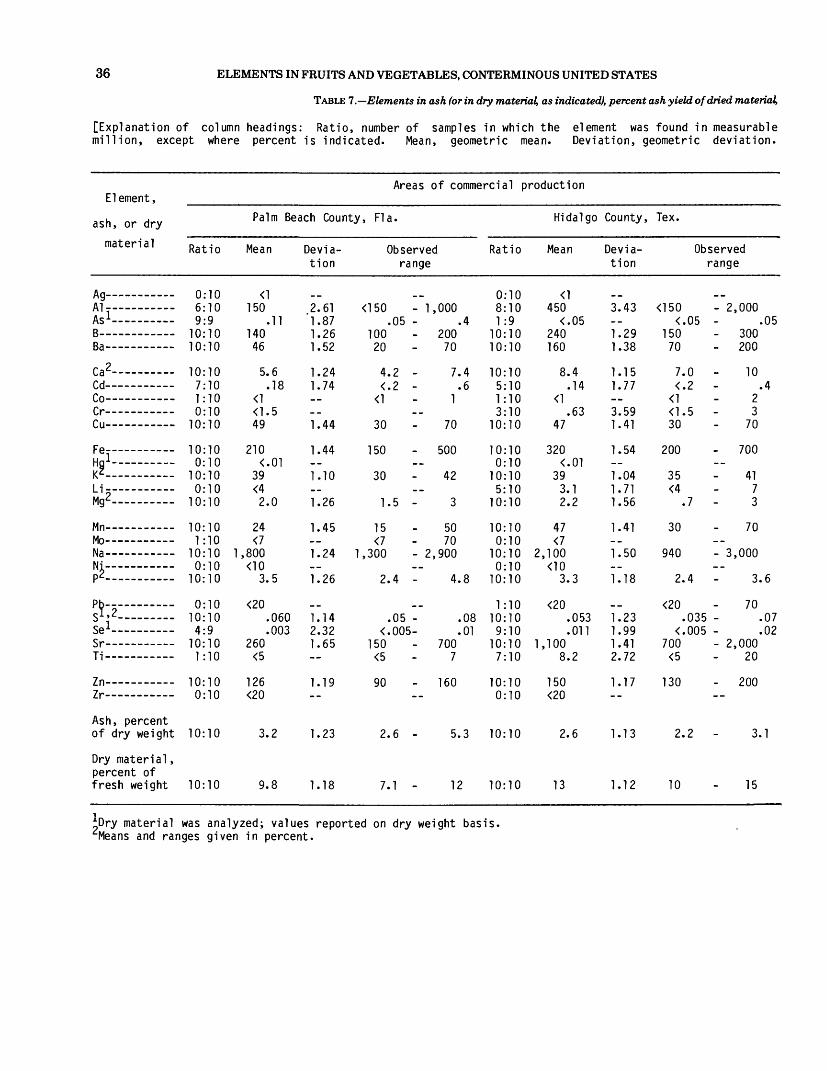
36 ELEMENTS IN FRUITS AND VEGETABLES, CONTERMINOUS UNITED STATES
TABLE 7.—Elements in ash (or in dry material, as indicated), percent ash yield of dried material,
[Explanation of column headings: Ratio, number of samples in which the element was found in measurable million, except where percent is indicated. Mean, geometric mean. Deviation, geometric deviation.
Element,
ash, or dry material
A 0_ __ ________rtg_
Al _ __ ________HI- —————
As 1 _______
Ra__ __ _______
Ca 2_______/> _iCo--— — —fr-----------Cu —————————
Fe ———————HnlH g ———————————1^2Li- — — — -Mg^ ———————
MM
Mo ———————NaNi-----------lN i ——————————p2 ————————
DK __ ___ _ _Sl,2—— — --Se 1 -— — —Sr-----------Ti ————————
Zn ———————7—
Ash, percent of dry weight
Dry material , percent of fresh weight
k)ry material
Areas of commercial production
Palm Beach County,
Ratio
0:10 6:10 9:9
10:10 10:10
10:10 7:10 1:10 0:10
10:10
10:10 0:10
10:10 0:10
10:10
10:10 1:10
10:10 0:10
10:10
0:10 10:10 4:9
10:10 1:10
10:10 0:10
10:10
10:10
Fla.
Mean Devia tion
<1 150
140 46
5.
<r<1. 49
210 <.
39 <4 2.
24 <7
1,800 <10
3.
<20
260 <5
126 <20
3.
9.
was analyzed;
2.61 <150 11 1.87
1.26 100 1.52 20
6 1.24 4 18 1.74 <
<1 5
1.44 30
1.44 150 01
1.10 30
0 1.26 1
1.45 15 <7
1.24 1,300
5 1.26 2
060 1.14 003 2.32 <
1.65 150 <5
1.19 90
2 1.23 2
8 1.18 7
values reported on
Observed range
- 1,000 .05 -
- 200 70
.2 - 7.
.2 - 1
70
- 500
42
.5 - 3
50 70
- 2,900
.4 - 4.
.05 -
.005- - 700
7
- 160
.6 - 5.
.1 - 12
dry weight
Ratio
0:10 8:10
4 1:9 10:10 10:10
4 10:10 6 5:10
1:10 3:10
10:10
10:10 0:10
10:10 5:10
10:10
10:10 0:10
10:10 0:10
8 10:10
1:10 08 10:10 01 9:10
10:10 7:10
10:10 0:10
3 10:10
10:10
basis.
Hidalgo
Mean
<1 450
<.05 240 160
8.4 .14
<1 .63
47
320 <.01
39 3.1 2.2
47 <7
2,100 <10
3.3
<20 .053 .011
1,100 8.2
150 <20
2.6
13
County,
Devia tion
3.43
1.29 1.38
1.15 1.77
3.59 1.41
1.54
1.04 1.71 1.56
1.41
1.50
1.18
1.23 1.99 1.41 2.72
1.17
1.13
1.12
Tex.
<150 <.
150 70
7. <.
<1 <1. 30
200
35 <4
30
940
2.
<20
<.700
<5
130
2.
10
Observed range
- 2,000 05 - .05
- 300 - 200
0 - 10 2 - .4
2 5 - 3
70
- 700
41 7
7 - 3
70
- 3,000
4 - 3.6
70 035 - .07 005 - .02
- 2,000 20
- 200
2 - 3.1
15

TABLES 4-121
and percent dried-material yield of fresh grapefruit from areas of commercial production
concentrations to number of samples analyzed. Means and ranges are given in parts per Leaders (--) in figure column indicate no data available]
37
Areas of commercial production
Riverside County, Calif.
Ratio
0:1010:101:8
10:1010:10
10:108:102:105:10
10:10
10:100:10
10:107:10
10:10
10:102:10
10:105:10
10:10
0:1010:109:10
10:1010:10
10:100:10
Mean
<1810
<.05150
71
6.9.22.46
1.361
560<.01
364.71.9
304.3
1,8007.53.3
<20.083.022
1,30019
150<20
Devia tion
2.35--1.21 .1.99
1.111.621.691.911.18
1.82--1.061.891.30
1.431.381.393.091.26
__1.092.301.452.11
1.18--
200<.
10030
6.<.
<1<1.50
300
34<4
1.
15<7
1,200<10
2.
.<.
7007
no
Observed range
- 3,00005 - .05
- 200- 150
0 - 8.22 - .4
15 - 3
70
- 2,000--
4011
5 - 3
507
- 3,00070
4 - 4.8
__070 - .095005 - .06
- 2,00030
- 200--
Ratio
0:109:106:10
10:1010:10
10:103:100:100:10
10:10
10:100:10
10:1010:1010:10
10:100:10
10:100:10
10:10
0:1010:1010:1010:104:10
10:100:10
(continued)
Yuma
Mean
<1350
.044180
70
3.6.11
<1<1.542
240<.01
29121.5
37<7
1,300<10
2.0
<20.069.011
4703
97<20
County,
Devia tion
2.271.991.22.08
1.891.56----1.36
1.59--1.421.511.51
1.53--1.61__1.40
__1.121.341.825.10
1.44--
Ariz.
<150<.
15020
1.<.
30
150
155
•
20
600
1.
.
.200
<7
60
Observed range
- 1,00005 - .10
- 300- 150
2 - 7.22 - 2
_---
70
- 500--
4021
7 - 3
70--- 2,200--
2 - 3.6
__055 - .0801 - .02
- 1,00030
- 170--
10:10 4.4 1.12 3.9 5.1 10:10 5.6 1.39 3.5 11
10:10 10 1.06 9.1 11 10:10 8.6 1.13 10

38 ELEMENTS IN FRUITS AND VEGETABLES, CONTERMINOUS UNITED STATES
TABLE 8.—Elements in ash (or in dry material, as indicated), percent ash yield of dried material,
[Explanation of column headings: except where percent is indicated.
Ratio, number of samples in which the element was found in measurable Mean, geometric mean. Deviation, geometric deviation. Leaders (--)
El ement , ash, or dry
material
fin ____ ___ng — -------Ai_ _ _ _____Ml - — ------ Acl _______
p 3 Ba- ————r fl ^_____ _ _/> _J
Co ——————rr ___ _ __
fu-Fe ——— ----iHgl-- —— --i/Z1 •;__ _ _ _
Mg2 —————Mn —— - ——Mo —————NaNi —————
p2_________Pb-- ————S J-.2_______Sel— — -
Sr- _ - _ _ -Ti—— —— —Zn— — —Zr- — — -
Ash, percent of dry weight
Dry material , percent of fresh weight
*Dry material
Areas of commercial
Palm Beach County,
Ratio
0:10 5:10 0:10
10:10
10:10 10:10 6:10 3:10 3:10
10:10 10:10 0:10
10:10 0:10
10:10 10:10 0:10
10:10 0:10
10:10 0:10
10:10 1:9
10:10 0:10
10:10 0:10
10:10
10:10
Mean Devia tion
<1no
<.177
40 5.
50 338
<. 39 <4
2. 51 <7
1,300 <10
3. <20
<.
200 <5
150 <20
3.
12
was analyzed;
5.42 05
1.57
1.52 8 1.16 17 3.77 57 1.56 56 4.09
1.61 1.46
01 1.05
5 1.41 1.64
1.53
3 1.19
060 1.12 005 --
2.49
1.26
3 1.09
1.12
<150
70
20 4. <.
<1 <1.
20 300
37
1. 30
700
2.
<.
20
110
2.
10
values reported
Fla.
Observed range
- 3,000
- 300
70 7 - 7.4 2 - 2.5
1 5 - 7
70 - 1,000
42
5 - 5 - 150
- 2,200
4 - 3.6
05 - .075 005 - .005
- 500
- 240
8 - 3.6
15
on dry weight
production
Hidalgo County, Tex.
Ratio
0:10 10:10
0:9 10:10
10:10 10:10 4:10 2:10 1:10
10:10 10:10 0:10
10:10 4:10
10:10 10:10 1:10
10:10 0:10
10:10 1:10
10:10 9:10
10:10 6:10
10:10 1:10
10:10
10:10
basis.
Mean
<1630
<.05 280
220 8.6
.13
.46 <1.5
47 360
<.01 38 2.8
2.2 50 <7
1,300 <10
2.9 <20
.064
.0089
1,100 5.3
140 <20
3.1
14
Devia tion
2.65
1.32
1.44 1.19 1.46 1.69
1.42 1.49
1.06 1.83
1.33 1.36
1.38
1.30
1.12 1.42
1.46 3.16 1.22
1.15
1.09
200
200
150 7. <.
<1 <1.
30 300
35 <4
1. 30 <7
700
1. <20
<.
700 <5
120 <20
2.
12
Observed range
- 3,000
- 500
- 500 2 - 12 2 -
1 5 - 3
70 - 1,000
42 6
5 - 3 70
7 - 2,600
8 - 3. 20
055 - 01 -
- 2,000 30
- 200 20
7 - 4.
16
2
6
075 01
4
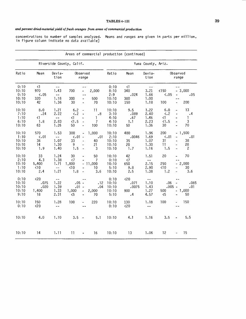
TABLES 4-121
and percent dried-material yield of fresh oranges from areas of commercial production
concentrations to number of samples analyzed. Means and ranges are given in parts per million, in figure column indicate no data available]
39
Areas of commercial production (continued)
Riverside County, Calif.
Ratio
0:1010:100:10
10:1010:10
10:107:101:106:10
10:10
10:101:10
10:1010:1010:10
10:102:10
10:101:10
10:10
0:1010:1010:1010:109:10
10:100:10
Mean
<1970
<.05320
42
8.0.24
<11.8
63
570<.01
36141.9
334.3
5,400<10
2.4
<20.075.020
1,40018
150<20
Devia tion
__1.43--
1.181.36
1.212.22--
2.831.26
1.53_-
1.071.301.40
1.241.381.71--
1.21
__1.221.391.332.31
1.28--
Observed range
700
30030
6.2<.2
<1<1.550
300<.01
3391.5
30<7
1,800<10
1.8
.05
.011,000
<5
100
__- 2,000--
50070
11.8
17
100
- 1,000.01
4021
3
507
- 11,000103.6
_ _
.12
.04- 2,000
70
220--
Ratio
0:108:102:9
10:1010:10
10:103:104:104:10
10:10
10:102:10
10:1010:1010:10
10:100:10
10:105:10
10:10
0:1010:1010:1010:10
5:10
10:100:10
Yuma
Mean
<1340
.024300150
9.5.089.67
1.150
480.0046
3520
1.7
42<7
6509.82.5
<20.071.0075
900.4
130<20
County, Ariz.
Devia tion
__3.211.661.001.18
1.222.401.462.231.36
1.961.691.071.301.16
1.51--
2.152.901.38
_ _
1.101.431.274.57
1.18--
Observed range
<150<.05
100
6.0<.2
<1<1.530
200<.01
3111
1.5
20
250<10
1.2
.06
.005500
<5
100
__
- 3,000.05
--- 200
13.4
13
70
- 1,500.01
3828
2
70--- 2,000
303.6
_ _.085.01
- 1,00050
- 150--
10:10 4.0 1.10 3.5 - 5.1 10:10 4.1 1.16 3.5 5.5
10:10 14 1.11 11 16 10:10 13 1.06 12 15

40 ELEMENTS IN FRUITS AND VEGETABLES, CONTERMINOUS UNITED STATES
TABLE 9.—Elements in ash (or in dry material, as indicated), percent ash yield of dried material,
[Explanation of column headings: Ratio, number of samples in which the element was found in measurable million except where percent is indicated. Mean, geometric mean. Deviation, geometric deviation.
Element, ash, or dry
material
An ___ _ __«yAT __ _ ____ttl-flcl ________R__ __ _ _ _r>.
Ca2— — -p_iCo—— — -rr ______ _Cu — — ——
Fer— - — H n ia --------VL.
Li- ——— —Mg2 —————
Mn — — ——Mo —— ———Ma-Ni— — —P^_
Ph._— — —s i> 2— —_Se 1 — -- -Sr- _ - _ __Ti— ————
Zn ——————7w.
Ash, percent of dry weight
Dry material, percent of fresh weight
Areas of commercial
Ratio
0:10 7:10 5:10
10:10 10:10
10:10 10:10 3:10 5:10
10:10
10:10 5:10
10:10 0:10
10:10
10:10 0:10
10:10 4:10
10:10
1:10 10:10 5:10
10:10 3:10
10:10 0:10
10:10
10:10
Wayne
Mean
<1240
.036 300
18
.30
.86
.45 1.2
83
240 .0071
18 <4 .97
61 <7
140 7.4 1.3
<20 .068 .0036
27 <5
no<20
7.2
6.9
County
Devia tion
, N.
3.39 <150 2.06 <. 1.75 150 1.52 7
1.52 2.42 2.40 <1 4.52 <1. 1.92 30
1.92 70 1.78 <. 1.50 12
1.32
1.77 20
2.00 50 1.79 <10 1.81
-- <20 1.52 1.90 <. 1.55 15
<5
1.83 50
1.55 3.
1.57 3.
Y.
Observed range
- 2,000 05 - .10
- 1,000 30
16 - .58 60 - 3.0
2 5 - 15
- 200
- 700 01 - .02
36
50 - 1.7
150
- 350 15
32 - 2.4
20 035 - .12 005 - .02
70 30
- 250
0 - 14
6 - 12
Ratio
0:10 10:10 2:10
10:10 10:10
10:10 6:10 5:10 9:10
10:10
10:10 1:10
10:10 1:10
10:10
10:10 0:10
10:10 7:10
10:10
1:10 10:10 6:10
10:10 10:10
10:10 0:10
10:10
10:10
production
Yak i ma
Mean
<11,200
.013 560
55
.49
.18
.69 3.2
70
750 <.01
20 <4 1.5
78 <7
190 15 2.4
<20 .029 .0044
82 61
122 <20
8.9
14
County
Devia tion
2.67 3.31 1.38 2.64
2.01 2.43 2.15 2.16 1.56
1.77
1.75
1.51
1.67
1.91 2.92 1.56
1.32 1.99 2.14 2.45
1.87
1.70
1.12
, Wash.
Observed range
200 - 7,000 <.05 -
300 - 1,000 15 - 200
.20 - 1. <.20 -
<1 - 1 <1.5 - 10 30 - 150
300 - 2,000 <.01 - 8.5 - 43
<4 - 4 .70 - 3.
30 - 150
100 - 450 <10 - 70
1.2 - 4.
<20 - 20 .02 -
<.005 - 30 - 300 15 - 200
<15 - 300
1.5 - 9
12 - 17
10
2 60
01
0
8
045 01
*Dry material was analyzed; values reported on dry weight basis. ^Means and ranges given in percent.
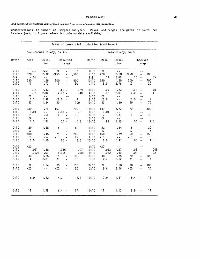
TABLES 4-121
and percent dried-material yield of fresh peaches from areas of commercial production
concentrations to number of samples analyzed. Means and ranges are given in parts per Leaders (--), in figure column indicate no data available]
41
Areas of commercial production (continued)
San Joaquin County, Calif.
Ratio
2:109:100:9
10:1010:10
10:104:100:105:10
10:10
10:101:10
10:100:10
10:10
10:100:10
10:106:10
10:10
0:1010:102:10
10:108:10
10:101:10
Mean
.36520
<.05350
17
.18
.12<1
1.353
330<.01
19<41.0
29<7
180101.5
<20.051.0023
4214
71<20
Devia tion
2.692.32--
1.281.72
1.432.01--
1.921.54
1.78--
1.51--
1.37
1.58--
1.451.571.65
__1.281.691.852.83
1.64—
Observed range
<1<150
__300
7
.10 -<.20 -
--<1.5 -30
150<.01 -
11-_
.70 -
15--
75<10
.60 -
__.035-
<.005-15<5
35<20
21,500
50030
.29
.40
3100
700.01
35
1.5
50
260153.6
.07
.005100
50
13030
Ratio
0:107:108:8
10:107:10
10:104:100:101:10
10:10
10:100:10
10:100:10
10:10
10:101:10
10:101:10
10:10
0:1010:1010:1010:103:10
10:102:10
Mesa County, Colo.
Mean
<1220
.17340
5.9
.27
.12<1<1.533
140<.01
17<4
.94
23<7
160<10
1.0
<20.033.012
482.7
719.6
Devia tion
__2.881.651.352.76
1.732.01----
1.50
1.72--
1.37_-
1.50
1.34_.
1.79--
1.47
_ _1.271.401.752.12
1.502.16
Observed range
__<150
.10 -300
<3
.12 -<.2 -
--<1.5 -20
70--
11--
.50 -
15<750
<10.60 -
_ _.02 -.01 -
20<5
30<20
700.35
70020
.70
.4
770
300
33
2.0
307
350101.8
.045
.02100
7
10030
10:10 6.0 1.22 4.3 - 8.2 10:10 7.9 1.41 5.4 15
10:10 11 1.39 6.4 - 17 10:10 11 1.13 9.9 14
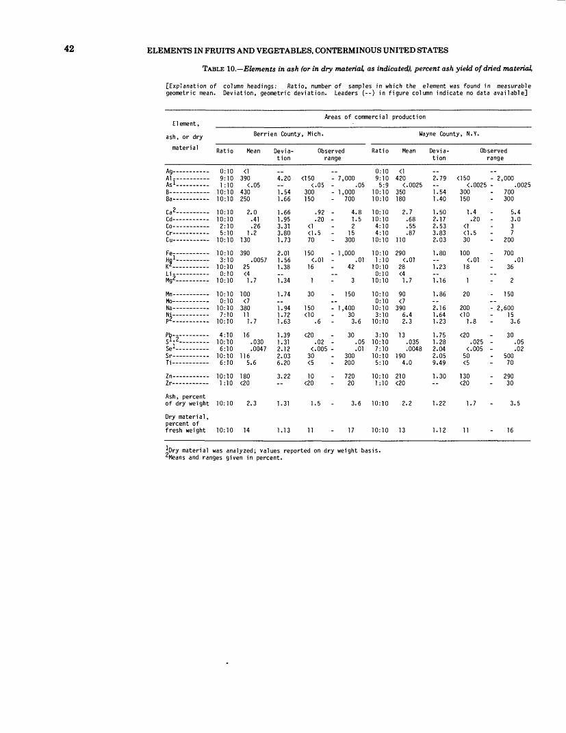
42 ELEMENTS IN FRUITS AND VEGETABLES, CONTERMINOUS UNITED STATES
TABLE 10.— Elements in ash (or in dry material, as indicated), percent ash yield of dried material,
[Explanation of column headings: Ratio, number of samples in which the element was found in measurable geometric mean. Deviation, geometric deviation. Leaders (--) in figure column indicate no data available]
Element,
ash, or dry
Areas of commercial production
Bern' en County, Mich. Wayne County, N.Y.
mater1a1 Ratio Mean
Ag ——————— 0:10 <1 Ai___ _ _ _ _ 9-10 390As 1 —————— l':10 <.05B ———————— 10:10 430p,a —————— _ in-in ?i;n
Devia- Observed Ratio Mean Devia- Observed tion range tion range
0:10 <14.20 <150 - 7,000 9:10 420 2.79 <150 - 2,000
<.05 - .05 5:9 <.0025 — <.0025 - .00251.54 300 - 1,000 10:10 350 1.54 300 - 700i fifi i«;n _ 7nn in-in ian i.an iRn _ "?nn
Ca 2—————— 10:10 2.0Cd—————— 10:10 .41Co——————— 2:10 .26Cr——————— 5:10 1.2Cu——————— 10:10 130
Fe-—————— 10:10 390Hgl—————— 3:io .0057KZ——- — 10:10 25Li-—————— 0:10 <4Mg2—————— 10:10 1.7
Mn——————— 10:10 100Mo——————— 0:10 <7Na——————— 10:10 380Ni——————— 7:10 11pt——————— 10:10 1.7
16fc ——— 4:10——— 10:10 .030
Se 1 —————— 6:10 .0047Sr——————— 10:10 116Ti——————— 6:10 5.6
Zn- Zr-
10:10 180 1:10 <20
Ash, percentof dry weight 10:10 2.3
Dry material, percent of fresh weight
1.661.953.313.801.73
2.011.561.38
1.34
1.74
1.941.721.63
1.391.312.122.036.20
.92 -
.20 -
70
150
16
30
4.81.52
15300
- 1,000.
42.01
150 - 1
.6
150
,400303.6
10:1010:104:104:10
10:10
10:10 1:10
10:10 0:10
10:10
10:10 0:10
10:10 3:10
10:10
2.7.68.55.87
110
290<.01
28 <41.7
90<7
390 6.4 2.3
<20.02 -
<.005 - 30 <5
30 3:10 13
300200
.05 10:10
.01 7:1010:10 190 5:10 4.0
.035
.0048
10:10 14
3.22 10 <20
1.31 1.5
1.13 11
720 10:10 210 20 1:10 <20
3.6 10:10 2.2
1.502.172.533.832.03
1.80
1.23
1.16
1.86
2.161.641.23
1.751.282.042.059.49
1.4.20
<1<1.5 30
100<.01
18
1
20
200 <10
1.8
<20.025
<.005 50 <5
17 10:10 13
1.30 130 <20
1.22 1.7
1.12 11
5.43.037
200
.01700
36
2
1 50
- 2,600 15 3.6
30.05 .02
50070
29030
3.5
16
*Dry material was analyzed; values reported on dry weight basis. Means and ranges given in percent.
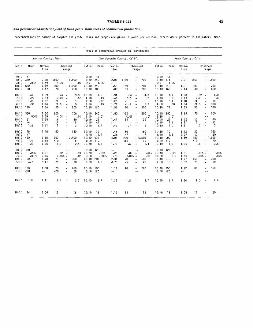
TABLES 4-121 43
and percent dried-material yield of fresh pears from areas of commercial production
concentrations to number of samples analyzed. Means and ranges are given in parts per million, except where percent is indicated. Mean,
Areas
Yakima County, Wash.
Ratio
0:108:103:10
10:1010:10
10:107:107:104:10
10:10
10:102:10
10:101:10
10:10
10:100:10
10:104:10
10:10
0:1010:107:10
10:105:10
10:101:10
Mean
<1320
.032580120
1.4.22
1.0.95
no330
.004621<41.5
79<7
4207.41.5
<20.026.0070
1504.7
120<20
Devia tion
__2.881.491.391.47
1.592.031.972.761.64
1.501.691.28—1.21
1.46—1.881.651.35
__1.212.661.709.11
1.60--
Observed range
<150<.05
30070
.74<.20
<1<1.550
200<.01
16<4
1
50
250<10
1.2
.02<.005
70<5
70<20
__- 1,500
.05- 1,000- 200
3.0.60
35
- 200
700.01
3052
- 150_-- 2,400
152.4
__.03.02
30070
- 26020
Ratio
0:108:100:9
10:1010:10
10:104:107:102:10
10:10
10:101:10
10:100:10
10:10
10:102:10
10:101:10
10:10
0:1010:105:10
10:103:10
10:100:10
of commercial production (continued)
San Joaquin County, Calif.
Mean
<1240
<.05340100
1.6.13.87.75
120
240<.01
21<41.4
791.4
970<10
1.4
<20.031.0035
2001.8
100<20
Devia tion
__2.05._1.521.83
1.941.461.251.791.55
1.50__1.44-_1.42
1.461.384.06—1.73
__1.261.782.314.78
1.77--
Observed range
<150
15030
.52<-2
<1<1.570
150<.01
15
.7
50<7
200<10
.6
.02<.005
70<5
40
__- 700..- 700- 200
4.0.2
11.5
- 300
- 500.01
35._
2
- 1507
- 6,600102.4
__.045.01
- 50020
- 220--
Ratio
0:108:100:9
10:1010:10
10:107:10
10:104:10
10:10
10:101:10
10:1010:1010:10
10:106:10
10:102:10
10:10
0:1010:1010:1010:107:10
10:100:10
Mesa County, Colo.
Mean
<1374
<.05540160
1.7.21
3.1.60
78
250<.01
217.31.0
707.3
900<10
1.3
<20.023.012
2708.9
150<20
Devia tion
__2.71—1.312.13
1.902.131.781.841.33
1.89-_1.621.471.51
1.722.071.49-.1.95
__1.311.601.773.32
1.72--
Observed range
<150
30030
.82<.2
<1<1.550
70
105
.7
30<7
400<10
.6
.015
.005150
<5
80
__- 1,500-_- 700- 500
4.0.6
10100
- 100
- 500--
4017
3
- 15020
- 1,600703.6
_..035.035
- 70030
- 350--
10:10 1.9 1.11 1.7 2.3 10:10 2.7 1.33 3.7 10:10 1.7 1.34 1.0 2.6
10:10 14 1.06 13 16 10:10 16 1.12 13 18 10:10 18 1.08 16 20

44 ELEMENTS IN FRUITS AND VEGETABLES, CONTERMINOUS UNITED STATES
TABLE II.—Elements in ash (or in dry material, as indicated), percent ash yield of dried material,
[Explanation of column headings: Ratio, number of samples in which the element was found in parts per million except where percent is indicated. Mean, geometric mean. Deviation, geometric
Element, ash, or dry
material
An-- ---Al - _--_As — — —
D-,
Ca 2 -r* jCd- — ------Co ——————(Y-- -------Cu—— ------
Fe— — —Hn 1 - __ ____l/ZLi- — - —
Mo ——————Ma
Nj— — —
Pb— ————
Sel— .....Sr- — - — - —Ti — —— — —
Zn ——————7.x.
Ash, percent of dry weight
Dry material , percent of fresh weight
Areas of commercial
Berrien County, Mich.
Ratio
1: 8: 4:
10: 10:
10: 7: 0: 4:
10:
10: 4:
10: 0:
10:
10: 0:
10: 2:
10:
2: 10: 8:
10: 5:
10: 0:
10:
10:
10 10 9 10 10
10 10 10 10 10
10 10 10 10 10
10 10 10 10 10
10 10 10 10 10
10 10
10
10
Mean
290 .025
280 54
.45
.19
1.0 77
220 .007
15 <4
.90
100 <7 95 6.6
.84
<20 .036 .0051
59 4.2
126
6.2
12
Devia tion
2.21 3.07 1.36 2.54
1.21 1.66
2.19 1.64
1.36 1.46 1.25
1.35
1.42
1.57 1.33 1.99
1.35 1.54 2.35 2.97
1.63
1.67
1.29
Observed range
<150 - 1
150 10
.35 -
30*
150
11
.5 -
50
50
.6 -
<20 .025 -
<.005 - 15 <5
65
2.6 -
8.0 -
3 ,000
.33 500 200
.66
.4
3 200
300 .01
20
1
150
200 10 2.4
70 .055 .01
150 20
280
17
16
Ratio
1:10 6:10 1:8
10:10 10:10
10:10 5:10 1:10 4:10
10:10
10:10 1:10
10:10 0:10
10:10
10:10 0:10
10:10 0:10
10:10
0:10 10:10 6:10
10:10 3:10
10:10 0:10
10:10
10:10
production
Wayne County, N.Y.
Mean
150320*
25
.65
.14
.89 92
280
15 <4
1.1
62 <7
163
1.3
<20 .037 .0042
82 <5
208
3.9
12
Devia tion
2.28
1.57 2.25
1.54 1.78
3.29 1.89
1.58
1.27
1.42
1.62
1.63
1.85
1.32 1.83 2.04
2.64
1.41
1.30
Observed range
<150150*
7
.32
30
150
9
.7
30
100
.6
.025 <.005
30 <5
30
2.2
6.7
- 1.5 - 700
.10 - 700 - 150
- 1.2 .4
- 1 - 7 - 200
- 500 .01
- 22
- 2
- 100
- 320
- 2.4
.05
.01 - 300 - 20
- 770
- 6.6
- 17
*Dry material was analyzed; values reported on dry weight basis. Means and ranges given in percent.

TABLES 4-121
and percent dried-material yield of fresh plums from areas of commercial production
measurable concentrations to number of samples analyzed. Means and ranges are given in Leaders (--) in figure column indicate no data available]
45
Areas of commercial production (continued)
Ratio
1:108:100:8
10:1010:10
10:103:101:102:10
10:10
10:100:10
10:100:10
10:10
10:100:10
10:101:10
10:10
1:1010:10
5:1010:10
7:10
10:101:10
Yakima
Mean
<1290
<.05610
60
.62
.11<1
.5133
270<.01
16<41.2
45<7
125<10
1.3
<20.029.0036
12012
100<20
County
Devia tion
__2.50--
1.513.55
1.411.56--
2.771.50
1.62--
1.30_-
1.24
1.46--
1.61--
1.64
_ _1.182.901.684.72
1.82--
, Wash.
Observed range
<-|
<150
30020
.41<.2
<1<1.520
150
10
1
30
50<10
.6
<20.025
<.00570<5
40<20
3- 1,500--- 1,500- 1,500
1.2.2
23
70
- 500--
26_-
1.5
70-_- 250
102.4
70.04.02
- 300- 150
26020
Ratio
1:106:107:7
10:1010:10
10:101:100:101:10
10:10
10:100:10
10:100:10
10:10
10:108:10
10:100:10
10:10
7:1010:1010:1010:101:10
10:100:10
Mesa
Mean
<-|
160.59
34013
.60<.2
<1<1 .529
120<.01
18<41.0
277
110<10
.85
23.027.011
110<5
65<20
County,
Devia tion
_ _2.321.321.351.36
1.42------
1.46
1.57--
1.35--
1.29
1.511.261.70--
1.44
1.401.231.551.35--
1.43--
Colo.
Observed range
<1<150
.4300
7
.30<.2
<1 .515
50
12
.7
10<750
.6
<20.02.005
70<5
40
- 1.5- 500
.9- 700- 20
.86
.2--- 1.5- 50
- 200--- 26--- 1.5
- 50- 10- 250--- 1.2
- 30.4.02
- 150- 5
- 110--
10:10 4.3 1.21 3.4 5.9 10:10 5.1 1.13 4.3 6.0
10:10 17 1.13 13 19 10:10 18 1.06 17 20

46 ELEMENTS IN FRUITS AND VEGETABLES, CONTERMINOUS UNITED STATES
TABLE 12.—Elements in ash (or in dry material, as indicated), percent ash yield of dried material
[Explanation of column headings: Ratio, number of samples in which the element was found in measurable except where percent is indicated. Mean, geometric mean. Deviation, geometric deviation. Leaders (--)
Element, ash, or dry
material
An- _ _ ____«y-Al ___-__-__Ml - ————— ---AclR____ _ __ _Ra
Ca 2 -- -f* <JCd--- — ----Co— ———O--- _ __ _C U— ———
Fe ...He, 1 -——1^2
Mg 2 —————
Mn —————Mo — — —Ma
Ni--- _ _ __9p2___ ——— _
Pb— — —S l»2_______Se 1 — ———S r _ _ ____ _Ti ——————
Zn— — —Zr —————
Ash, percent of dry weight
Dry material , percent of fresh weight
Areas of commercial production
Berrien County, Mich.
Ratio
0:2 0:2 0:2 2:2 2:2
2:2 2:2 0:2 0:2 2:2
2:2 0:2 2:2 0:2 2:2
2:2 2:2 2:2 0:2 2:2
0:2 2:2 2:2 2:2 0:2
2:2 0:2
2:2
2:2
Mean
<} <150
<.05 120 150
6.6 .80
<1 <1.5 39
390 <.01
40 <4 1.7
150 15
4,500 <10
3.6
<20 .58 .11
200 <5
273 <20
9.3
7.3
Devia- Observed tion range
1.33 100 - 150 1.00
1.09 6.2 - 7.0 1.00
1.44 30 - 50
1.44 300 - 500
1.00
1.23 1.5 - 2
1.00 1.00 1.28 3,800 - 5,400
1.00
1.09 .55 - .62 4.16 .04 - .3 1.00
1.36 220 - 340
1.10 8.7 - 10
1.02 7.2 - 7.4
Ratio
0:2 2:2 2:2 2:2 2:2
2:2 2:2 1:2 0:2 2:2
2:2 0:2 2:2 0:2 2:2
2:2 2:2 2:2 0:2 2:2
0:2 2:2 2:2 2:2 1:2
2:2 0:2
2:2
2:2
Cumberland County
Mean
<1 200
.05 122 200
7.7 1.7
<1 <1.5 24
500 <.01
38 <4 3.2
122 15
4,700 <10
3.6
<20 .82 .057
300 <5
295 <20
12
5.5
Devia tion
1.00 1.00 1.33 1.00
1.02 1.23
1.33
1.00
1.02
1.91
1.33 1.00 1.13 4,
1.00
1.00 1.63 1.00
1.02
1.13
1.14
, N.J.
Observed range
100 - 150
7.6 - 7.8 1.5 - 2
<1 - 1.
20 - 30
38 - 39
2 - 5
100 - 150
300 - 5,100
.04 - .08
<5 - 10
290 - 300
11 - 13
5.0 - 6.0
material was analyzed; values reported on dry weight basis Means and ranges given in percent.
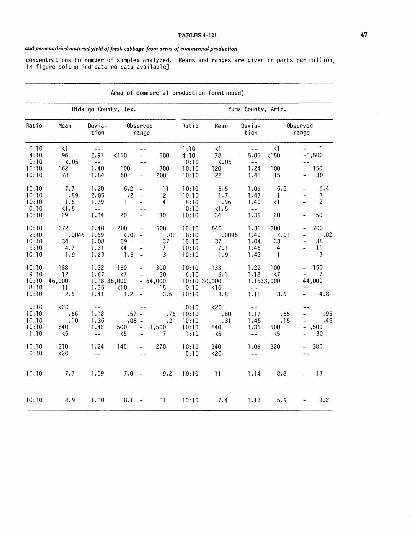
TABLES 4-121 47
and percent dried-material yield of fresh cabbage from areas of commercial production
concentrations to number of samples analyzed. Means and ranges are given in parts per million, in figure column indicate no data available]
Area of commercial production (continued)
Hidalgo County, Tex.
Ratio
0:104:100:10
10:1010:10
10:1010:1010:100:10
10:10
10:102:10
10:109:10
10:10
10:109:10
10:108:10
10:10
0:1010:1010:1010:101:10
10:100:10
Mean
<196
<.05162
78
7.7.59
1.5<1 .529
372.0046
344.71.9
18812
46,000112.6
<20.66.10
840<5
210<20
Deviation
__2.97--
1.401.54
1.202.051.79--
1.14
1.401.691.081.311.23
1.321.671.181.351.41
__1.121.361.42--
1.24--
Observedrange
__<150
--100 -50
6.2 -.2 -
1_-
20
200<.01 -
29<41.5 -
150<7
36,000 - 64<10
1.2 -
__.57 -.08 -
500 - 1<5
140--
500
300200
1124
30
500.01
3773
30030
,000153.6
.75
.2,500
7
270
Ratio
1:104:100:10
10:1010:10
10:1010:108:100:10
10:10
10:108:10
10:1010:1010:10
10:106:10
10:100:10
10:10
0:1010:1010:1010:10
1:10
10:100:10
Yuma County,
Mean
<178
<.05120
22
5.51.7.96
<1 .534
540.0096
377.11.9
1336.1
30,000<10
3.8
<20.80.31
840<5
340<20
Deviation
__5.06--
1.241.41
1.091.471.40-_
1.35
1.311.401.041.451.43
1.221.181.1533--
1.11
_ _
1.171.451.36--
1.06-_
Ariz.
<1<150
10015
5.1
<1
20
300<.
3341
100<7
,000
3.
.
.500
<5
320
Observedrange
1-1,500--- 150- 30
2 - 6.432
--- 50
- 70001 - .02
- 38- 11
3
- 1507
44,000--
6 - 4.8
_ _55 - .9515 - .45
-1,500- 30
- 380--
10:10 7.7 1.09 7.0 - 9.2 10:10 11 1.14 13
10:10 1.10 8.1 11 10:10 7.4 1.13 5.9 9.2

48 ELEMENTS IN FRUITS AND VEGETABLES, CONTERMINOUS UNITED STATES
TABLE 13.—Elements in ash (or in dry material, as indicated), percent ash yield of dried material, and percent dried-material yield of freshcarrots from areas of commercial production
[Explanation of column headings: Ratio, number of samples in which the element was found in measurable concentrations to number of samples analyzed. Means and ranges are given in parts per million, except where percent is indicated. Mean, geometric mean. Deviation, geometric deviation. Leaders (--) in figure column indicate no data available]
Element, ash, or dry
material
.Al - - Al--- ------Ac-1
D ->
Ca 2——r* -iCd- — — - —Co —— - — —Tr---------C U ——— —— —
Fe- — — —
K §Li ——————
Mn —————Mo — — —
P^Pb ———— -_
s e i— — -Ti ————— -Zn —————
Ash, percent of dry weight
Dry material , percent of fresh weight
Areas of commercial production
Ratio
0:10 7:10 7:7
10:10 10:10
10:10 10:10 2:10 0:10
10:10
10:10 2:10
10:10 0:10
10:10
10:10 0:10
10:10 10:10 0:10
10:10 10:10 10:10 2:10
10:10
10:10
10:10
Hidalgo County
Mean Devia tion
180
130 270
31
66
210
40 <4
1
164 <7
3,500 1
<20
753
7
11
2.00 .067 1.45
1.23 1.54
.6 1.14
.3 2.60
.46 1.70
1.45
1.30 .0066 1.46
1.05
.2 1.53
1.33
1.21 3 .9 1.54
.11 1.15
.032 1.40 1.25
.6 1.16
1.09
, Tex.
Observed range
<150 .05 -
100 200
3.0 - .2 -
50
150
36
.5 -
100
,000 - 4 .06 -
.09 -
.02 - 500 - 1
<5 75
6.2 -
9.3 -
700 .1
150 500
5.0 4 1
150
300 .01
42
2
300
,600 2.4
.15
.04 ,000
15
9.9
12
Ratio
0:10 2:10 2:9
10:10 10:10
10:10 10:10 3:10 0:10
10:10
10:10 2:10
10:10 6:10
10:10
10:10 0:10
10:10 10:10 0:10
10:10 10:10 10:10 0:10
10:10
10:10
10:10
Imperial
Mean
67 .024
157 50
3.5 3.4 .57
63*
230 .0046
39 3.5 1.4
94 <7
6,700 2.8
<20
.15
.13 820
<5 417
6.7
13
County,
Devia tion
2.09 1.66 1.23 1.65
1.12 1.69 1.56
1.26
1.22 1.68 1.05 1.47 1.33
1.35
1.22 i 1.23
1.17 1.50 1.42
1.10
1.08
Calif.
Observed range
<150 <.05 -
100 30
3.0 - 1
50
200
34 <4
.7 -
70
1,900 - 7, 2.4 -
.12 -
.08 - 500 - 1,
5.8 -
11
200 .05
200 100
4.4 6 1
100
300 .01
40 6 2
150
200 3.6
.19
.25 500
800
7.8
14
Dry material was analyzed; values reported on dry weight basis. Means and ranges given in percent.
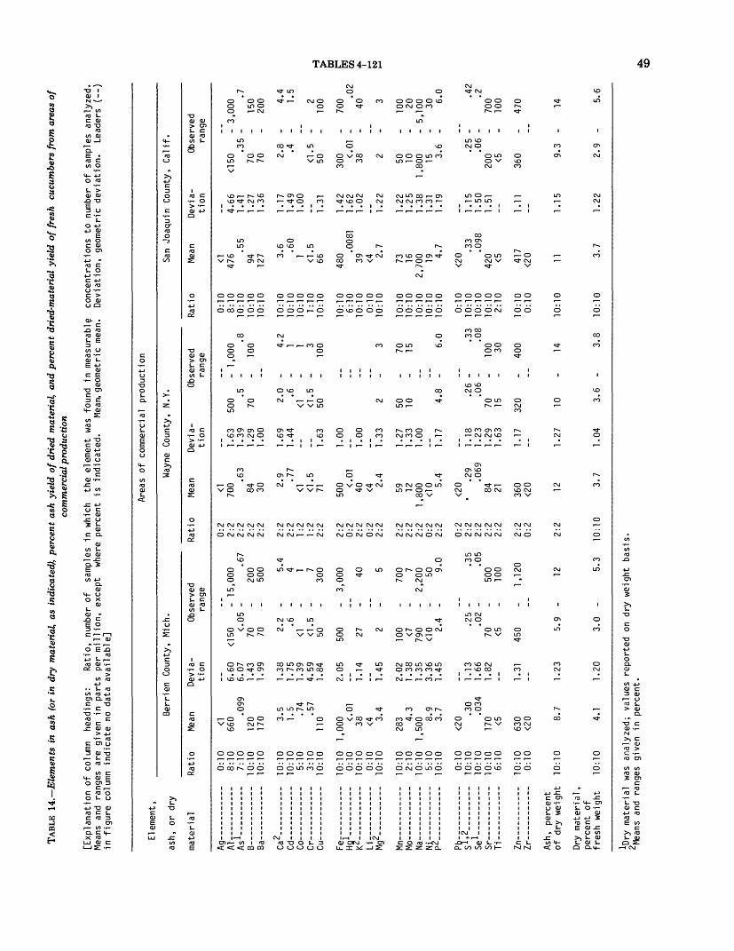
TABL
E 14
.—El
emen
ts i
n as
h (o
r in
dry
mat
eria
l, as
ind
icat
ed),
perc
ent a
sh y
ield
of d
ried
mat
eria
l, an
d pe
rcen
t dri
ed-m
ater
ial y
ield
of f
resh
cuc
umbe
rs fr
om a
reas
of
com
mer
cial
pro
duct
ion
[Exp
lana
tion
of c
olum
n he
adin
gs:
Rat
io,
num
ber
of
sam
ples
in
whi
ch
the
elem
ent
was
foun
d in
mea
sura
ble
conc
entr
atio
ns t
o nu
mbe
r of
sam
ples
an
alyz
ed.
Mea
ns a
nd r
ange
s ar
e gi
ven
in p
arts
pe
r m
illio
n,
exce
pt
whe
re p
erce
nt
is
indi
cate
d.
Mea
n, g
eom
etric
mea
n.
Dev
iatio
n,
geom
etric
dev
iatio
n.
Lead
ers
(--)
in
fig
ure
col
umn
indi
cate
no
data
ava
ilable
]
Elem
ent,
ash,
or
dry
Berr1en
Coun
ty' Mi
ch'
Areas
of c
ommercial
prod
ucti
on
Wayn
e Co
unty
, N.Y.
San
Joaquin
County,
Calif.
mat
eria
l
Ag—
— - —
Al—
——
——
— -
Ac
1-
__
__
__
__
.
R-,
r,2
Co —
——
——
— -
Cr
Cu —
——
——
-
i Hf
l1—
---
-- -
i/Z_
Li —
— _
_ —
.M
g2 —
——
——
— .
Mn —
——
——
•Mo
——
——
— •
Na —
——
——
-N
i— —
— •
P*- Pb
——
——
— .
cl,2
b
' —
——
— •
Sr —
——
——
•Ti
——
——
——
.
Zn —
— —
-7
r _
__
__
__
--.
Rat
io
--
0:10
8. i n
7:10
--
10:1
0--
10
:10
--
10:1
0--
10
:10
R-1
0--
3:
10--
10
:10
--
10:1
0--
0:
10--
10
:10
0:10
--
10:1
0
--
10:1
0--
2:
10--
10
:10
5:10
--
10:1
0
--
0:10
--
10:1
0--
10
:10
--
10:1
0--
6:
10
--
10:1
0n
-in
Mean <1 660
.099
120
170 3.
51.
5 .74
.57
110
1,00
0 <.01
QQ <4 3.
4
OQ
O 4 3
1,50
0 8.9
3 7
<20
.30 03
417
0 <5
con
<-?n
Dev
ia
tion
6.60
6.07
1.43
1.99
1 T
Q
1 7R
1 39
4 R9
Io
n
2 05
1.14
1 AR
2.02
1 ")
B
1 35
3.36
1 45
1.1
31
.66
1 Q
O
1.31
<150 <. 70 70 2. <1 <1
.50 500 27 2
100 <7 790
<10 2. *
70 <5 450
Obs
erve
d ra
nge
- 15
,000
05
- .6
720
050
0
2 -
5.4
6 -
4 15
- 7
300
- 3,
000 40 K
700 7
- 2,
200 50
4 -
9.0
25
- 35
02
- .0
550
010
0
1,12
0
Rat
io
0:2
2:2
2:2
2:2
2:2
2:2
2:2
1:2
1:2
2:2
2:2
0:2
2:2
0:2
2:2
2:2
2:2
2:2
0:2
2:2
0:2
2:2
2:2
2:2
2:2
2:2
n-?
Mea
n
<1 700
.63
Q/l 30 2.
9 .77
<1 <1.5
71 500 <.
0140 <4 2.
4
59 121,
800
<10 5
4
<20 .2
9.0
69Q
/l 21 360
<?n
Dev
ia
tion
1£Q
1 39
1.29
1.00
1.69
1.44
1/T
Q
1.00
1.00
1.33
1.27
1.33
1.00
1.17
1 1
Q
1 23
1.29
1.63
1.17
500 70 2. <1 <1
.R
fl 2 Rfl 10 4.
*
70 15
Obs
erve
d ra
nge
- 1,
000
5O
- 10
0
0 -
4.2
6 -
1 15
- 3
- 10
0 3 70 15
8r
n
9 a
o o
06
- .0
8-
100 30
- 40
0
Rat
io
0:10
8. i n
10:1
010
:10
10:1
0
10:1
010
:10
10:1
01:
1010
:10
10:1
06:
1010
:10
0:10
10:1
0
10:1
010
:10
10:1
010
:10
10:1
0
0:10
10:1
010
:10
10:1
02:
10
10:1
0n
-in
Mean
<1 476
RR94 12
7 3.6 .6
01 <1
.566 480
.008
139 <4 2.
7
73 162
,700 19 4.
7
<20 .3
3.0
9842
0 <5 417
<-?n
Dev
ia
tion
4.66
1.41
1.27
1.36
1.17
1.49
1.00
1.31
1.42
1/:o
1.02
1.22
1.22
1 ?R
1 Q
Q
1 31
1.19
1.15
1 R
fl1
Rl
1.11
<150 70 70 2 <1 R
fl
300 <
"3Q 2
Rfl 10
1,8
00 15 3
200 <R 360O
bser
ved
rang
e
- 3,
000
3R
- 7
150
- 20
0
.8
- 4.
44
- 1
R
50
100
- 70
0.0
1 -
.02
40 3
100 20
- 5,
100 30
.6
- 6.
0
r\c
o
- 70
0-
100
- 47
0Z
r
Ash,
pe
rcen
t o
f dr
y w
eigh
t
Dry
ma
teria
l ,
perc
ent
of
fre
sh
wei
ght
0:10
<2
0
10:1
0 8.
7
10:1
0 4.
1
0:2
<20
1.23
5.
9 -
12
2:2
12
1.20
3.
0 -
5.3
10:1
0 3.
7
0:10
<2
0
1.27
10
-
14
10:1
0 11
1.04
3.
6 -
3.8
10:1
0 3.
7
' *
' '
**u
w
~ i \J
1.15
9.
3 -
14
1.22
2.
9 -
5.6
k>ry m
aterial
was
analyzed;
valu
es r
eported
on d
ry w
eigh
t basis.
^Means a
nd r
ange
s gi
ven
in pe
rcen
t.
I 5 CO
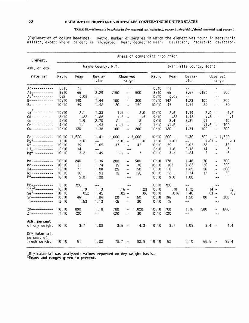
50 ELEMENTS IN FRUITS AND VEGETABLES, CONTERMINOUS UNITED STATES
TABLE 15.—Elements in ash (or in dry material, as indicated), percent ash yield of dried material, and percent
[Explanation of column headings: Ratio, number of samples in which the element was found in measurable million, except where percent is indicated. Mean, geometric mean. Deviation, geometric deviation.
Element,
ash, or dry
material
An--Al------- __
i Ac 1 - ___ __ __
Da
fa 2/"* ftCd- — --------Co——— -----O-- _ _______Cu—— — ——
Fe------ -----Ha 1
KzLi-- — — —
»j__Mn — ------- —Mo ———————
Mi— — -----P 2 __ ——— ____
s l,2_ 1sTi ———————~7«Zn-----------
Ash, percent of dry weight
Dry material , percent of fresh weight
Wayne County
Ratio
0:10 3:10 0:8
10:10 10:10
10:10 8:10 9:10 4:10
10:10
10:10 1:10
10:10 0:10
10:10
10:10 10:10 10:10 10:10 10:10
0:10 10:10 10:10 10:10 2:10
10:10 1:10
10:10
10:10
Mean
66 <.05
190 59
2.1 .22
1.9 1.1
130
1,500
39 <4 3.2
240 31 71 38 9.0
<20 .19 .022
46 .53
890
3.7
81
Devia tion
2.29
1.44 1.98
1.33 1.86 2.70 1.93 1.38
1.41
1.05
1.49
1.36 1.74 1.80 1.93 1.00
1.13 1.42 1.84 1.13
i-.io
1.08
1.02
Areas of
, N.Y.
Observed range
<150
100 20
1.5 -
100* -
1,000 - 3,
37* -
1.5 -
200 15 25 15
.16 -
.02 - 20 <5
780 - 1
3.5 -
78.7 -
commercial production
Twin Falls County, Idaho
500
300 150
3.0 .6
8 3
200
000 .01
43
7
500 70
150 150
.23
.06 150
30
,020
4.3
82.9
Ratio
0:10 3:10 0:10
10:10 10:10
10:10 9:10 9:10 1:10
10:10
10:10 1:10
10:10 2:10
10:10
10:10 10:10 10:10 10:10 10:10
0:10 10:10 10:10 10:10 0:10
10:10 0:10
10:10
10:10
Mean
65 <.05
142 47
2.5 .22
3.4120*
80039*
1.6 3.3
170 103
110 26 9.0
<20 .18 .016
196 <5
700
3.7
82
Devia tion
3.67
1.23 1.56
1.19 1.43 2.31
1.34
1.30
1.03 2.12 1.24
1.46 1.83 1.65 1.34 1.00
1.12 1.40 1.50
1.16
1.09
1.10
<150
100 20
2.
100
70038*
<4 3
70 30 50 15
100
580
3.
68.
Observed range
500
- 200 70
0 - 3.6 2 - .4
10 5 - 100
- 200
- 1,500 01 - .01
42 5 5
- 300 - 200 - 200
30
14 - .2 01 - .02
- 300
- 860
4 - 4.4
5 - 92.4
material was analyzed; values reported on dry weight basis, Means and ranges given in percent.

TABLES 4-121
dried-material yield of "fresh" (before oven drying) dry beans from areas of commercial production
concentrations to number of samples analyzed. Means and ranges are given in parts per Leaders (--) in figure column indicate no data available]
51
Areas of commercial production (continued)
San Joaquin County, Calif.
Ratio
2:105:100:8
10:1010:10
10:108:10
10:101:10
10:10
10:100:10
10:100:10
10:10
10:1010:1010:1010:1010:10
0:1010:1010:1010:104:10
10:100:10
Mean
<1<150
<.05150110
2.2.20
7.7<1.5
100
1,700<.01
39<43.5
20067837811
<20.21.020
2802.3
770<20
Devia tion
_ _----1.331.42
1.121.541.33--1.43
1.52--1.02--1.38
1.351.461.401.271.15
__1.151.001.521.89
1.06--
Observed range
<-|
<150
7070
1.8<.25
<1 .570
1,000
38
2
150505050
9
.18
150<5
700
3- 1,500--- 200- 150
2.6.4
122
- 200
- 3,000_-
40--
5
- 300- 100
150- 100
12
_ —
.28_-
500- 150
- 820--
Ratio-
0:104:100:9
10:109:10
10:1010:109:100:10
10:10
10:101:10
10:100:10
10:10
10:1010:1010:1010:1010:10
0:1010:1010:1010:101:10
10:100:10
Mesa County, Colo.
Mean
<!110
<.05137
29
4.5.45
10<1 .5
148
1,200<.01
38<43.3
180240
8354
9
<20.19.11
360<5
810<20
Devia tion
_ _1.99--1.263.27
1.151.501.40--1.58
1.36_-1.03_-1.24
1.261.352.201.461.00
_ _
1.081.651.59--
1.08--
Observed range
<150
100<3
3.8.2
6
70
700<.01
35
3
150150
2530
.17
.04200
<5
720
__- 300--- 200- 100
6.8
14--- 300
- 2,000.01
40--
5
- 300- 300- 300- 100--
_ _.22.2
- 70010
- 900--
10:10 4.0 1.04 3.7 - 4.2 10:10 4.2 1.07 4.0 4.9
10:10 1.04 80.3 - 91.5 10:10 90 1.04 82.9 - 93.7

52 ELEMENTS IN FRUITS AND VEGETABLES, CONTERMINOUS UNITED STATES
TABLE 16.—Elements in ash (or in dry material, as indicated), percent ash yield of dried material,
[Explanation of column headings: Ratio, number of samples in which the element was found in measurable except where percent is indicated. Mean, geometricic mean. Deviation, geometric deviation. Leaders (--) in
Element,
ash, or dry
material
n a _ _ _ __ ____Ay_ —— _ ——— ____
ni _ ________Ml- ---------- n<-l_ __ ____ _
D =>
fa 2P _iCo ———————r r_ _ _ _ _____Cu— — - — —
Fe--— — —H n ig —————————K z -_
Li-~~ ... —Mg^ ————————
Mn ———————Mo ———————WaNi ———————p2__-._______
Ph.. — __ ....Sl.2_________se i— — — -Sr- _ __ -.---Ti ___________
Zn ——— — —Zr ———————
Ash, percent of dry weight
Dry material, percent of fresh weight
Areas of commercial production
Cumberland County, N.J.
Ratio
0:10 10:10
6:6 10:10 10:10
10:10 10:10 4:10
10:10 10:10
10:10 7:10
10:10 3:10
10:10
10:10 1:10
10:10 5:10
10:10
2:10 10:10 10:10 10:10 10:10
10:10 10:10
10:10
10:10
Mean
<11 1 ,000
1.3 97
157
3.1 3.9
.53 22 36
4,500 .011
28 1.9 2.0
253 <7
2,200 8.8 1.5
11 .34 .078 .57
1,379
380 75
14
6.2
Devia tion
2.37 1.45 1.66 2.02
1.36 1.50 4.13 2.13 1.47
1.87 2.19 1.35 2.50 1.29
1.46
1.22 1.82 1.48
1.80 1.12 1.54 1.38 2.02
3.12 7.47
2.37
1.25
3,000
50 70
2. 1.
<1 7
20
2,000 <.
18 <4
1.
150 <7
1,600 <10
<20
100 500
150 20
18
3.
Observed range
- 30,000 5 - 2
300 500
0 - 4.6 5 - 6
4 70 50
- 15,000 01 - .04
40 8
5 - 3
500 7
- 2,900 20
6 - 2.4
30 29 - .4 04 - .2
200 - 3,000
- 3,360 300
29
7 - 8.0
Ratio
1:10 8:10 3:7
10:10 10:10
10:10 10:10 0:10 0:10
10:10
10:10 6:10
10:10 0:10
10:10
10:10 0:10
10:10 0:10
10:10
0:10 10:10 8:10
10:10 0:10
10:10 0:10
10:10
10:10
Palm
Mean
<1180
.034 85 84
5.3 .94
<1 <1.5 49
555 .0081
40 <4 1.4
255 <7
5,500 <10
3.6
<20 .22 .008
1,000 <5
680 <20
14
3.5
Beach County, Fla.
Devia tion
1.37 1.44 1.48 1.38
1.15 1.46
1.50
1.71 1.32 1.03
1.31
1.23
1.43
1.29
1.15 1.77 1.37
1.26
1.22
1.25
<1 <150
<.50 70
4.
30
300 <.
37
200
3,300
2.
<.700
460
11
2.
Observed range
2 - 300
05 - .05 - 150 - 150
5 - 6.6 6 - 2
- 100
- 2,000 01 - .01
40
7 - 2
- 300
- 9,200
4 - 4.8
16 - .25 005 - .02
- 2,000
- 920
20
9 - 5.7
Dry material was analyzed; values reported on dry weight basis. Means and ranges given in percent.

TABLES 4-121
and percent dried-material yield of fresh lettuce from areas of commercial production
concentrations to number of samples analyzed. Means and ranges are given in parts per million, figure column indicate no data available]
Areas of commercial production
53
Ratio
0:108:106:8
10:1010:10
10:1010:102:101:10
10:10
10:103:10
10:102:10
10:10
10:101:10
10:103:10
10:10
0:1010:1010:1010:104:10
10:100:10
Hidalgo County, Tex.
Mean Devia tion
<1362
.04490
113
5.02.6
.46<1.575
534.0057
391.51.8
181<7
25,0006.44.1
<20.29.077
6342.2
620<20
__2.661.221.291.30
1.121.701.70—1.16
1.411.561.042.461.47
1.57__1.22 201.641.15
__1.161.361.261.15
1.19--
<150<.
7070
3..
<1<1.70
300<.
37<4
1
70<7
,000<10
3.
.
.500
<5
420
Imperial County,
Observed range
__- 1,500
05 - .05150150
8 - 5.86 - 4
15 - 2
100
70001 - .01
4063
30015
- 36,00015
6 - 4.8
__24 - .3804 - .1
- 1,0007
800--
Ratio
0:107:101:8
10:1010:10
10:1010:104:102:10
10:10
10:108:10
10:108:10
10:10
10:100:10
10:107:10
10:10
0:1010:1010:1010:102:10
10:100:10
Mean
<1183
<.05100
13
3.98.7
.66
.5084
634.010
376.01.8
154<7
54,0009.33.9
<20.29.18
758<5
460<20
Devia tion
__1.84—1.201.61
1.171.361.463.001.21
1.261.031.051.601.26
1.10__1.11 461.131.13
__1.161.261.39—
1.13--
Calif.
Observed range
__<150
<.05 -70
7
2.8 -5
<1<1.5 -70
500 - 1<.01 -
34<41.5 -
150__
,000 - 64<10
3.6 -
__.22 -.10 -
500 - 1<5
340--
500.05
15030
4.814
13
100
,000.02
4093
200
,000104.8
.33
.2,500
20
530
10:10 13 1.22 11 19 10:10 13 1.15 10 16
10:10 3.6 1.17 2.9 - 4.8 10:10 3.8 1.17 3.3 - 5.3
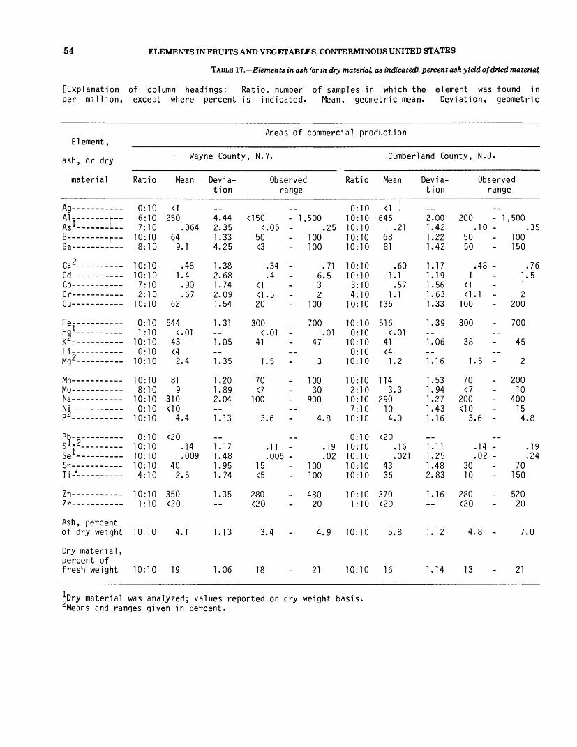
54 ELEMENTS IN FRUITS AND VEGETABLES, CONTERMINOUS UNITED STATES
TABLE 17.—Elements in ash (or in dry material, as indicated), percent ash yield of dried material,
[Explanation of column headings: Ratio, number of samples in which the element was found in per million, except where percent is indicated. Mean, geometric mean. Deviation, geometric
Element,
ash, or dry
material
.Al------- 4.
As 1 —— — L- B— — — t—
a2C" ACd- — --------Co———— ——r r_ _ ________Cu ————————
H n l
K ZLi- —— —— ——
Mn— —— -----Mo ———————
Nj— — ———
Pb ———————
s e i__________T' *
Zn ————— - —7 u%
Ash, percent of dry weight
Dry material , percent of fresh weight
Areas of commercial production
Wayne County, N.Y.
Ratio Mean Devia tion
0 6 7
10 8
10 10
7 2
10
01
10 0
10
10 8
10 0
10
0 10 10 10
4
10 1
10
10
*Dry material was Means and ranges
:10 250
:10 64 :10 9.
:10 1.
:10 62
:10 544
•10 43* :10 <4 :10 2.
:10 81 :10 9 :10 310
:10 4.
:10 <20
:10 40 :10 2.
:10 350 :10 <20
:10 4.
:10 19
analyzed given in
4.44 064 2.35
1.33 1 4.25
48 1.38 4 2.68 90 1.74 67 2.09
1.54
1.31
1.05
4 1.35
1.20 1.89 2.04
4 1.13
14 1.17 009 1.48
1.95 5 1.74
1.35
1 1.13
1.06
<150 <.
50 <3
20
300 41*
1.
70 <7
100
3.
15 <5
280 <20
3.
18
i values reported percent.
Observed range
- 1,500 05 - .25
- 100 - 100
34 - .71 4 - 6.5
3 5 2
- 100
- 700 01 - .01
47
5 - 3
- 100 30
- 900
6 - 4.8
11 - .19 005 - .02
- 100 100
- 480 20
4 - 4.9
21
on dry weight
Ratio
0:10 10:10 10:10 10:10 10:10
10:10 10:10 3:10 4:10
10:10
10:10 0:10
10:10 0:10
10:10
10:10 2:10
10:10 7:10
10:10
0:10 10:10 10:10 10:10 10:10
10:10 1:10
10:10
10:10
basis.
Cumberland County,
Mean
645 .21
68 81
.60 1.1
.57 1.1
135
51641*
<4 1.2
114 3.3
290 10 4.0
<20 .16 .021
43 36
370 <20
5.8
16
Devia tion
2.00 1.42 1.22 1.42
1.17 1.19 1.56 1.63 1.33
1.39
1.06
1.16
1.53 1.94 1.27 1.43 1.16
1.11 1.25 1.48 2.83
1.16
1.12
1.14
200
50 50
1
100
300
38
1.
70 <7
200
3.
30 10
280 <20
4.
13
N.J.
Observed range
- 1,500 10 - .35
- 100 - 150
48 - .76 1.5 1
1 - 2 - 200
700
45
5 - 2
- 200 10
- 400 15
6 - 4.8
14 - .19 02 - .24
70 - 150
520 20
8 - 7.0
21
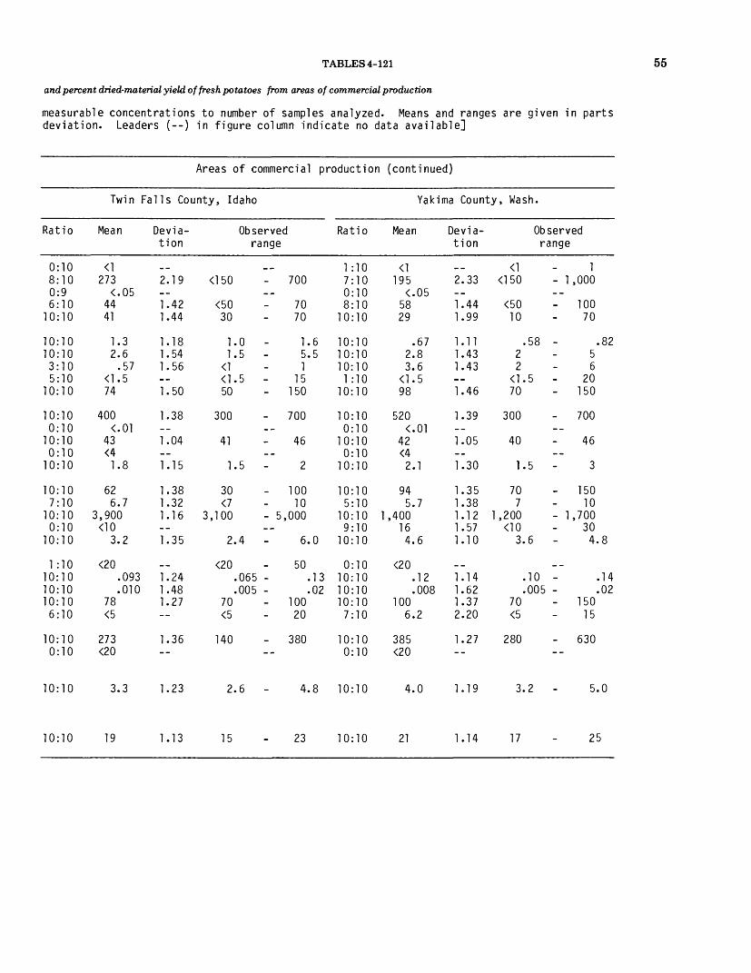
TABLES 4-121
and percent dried-material yield of fresh potatoes from areas of commercial production
measurable concentrations to number of samples analyzed. Means and ranges are given in parts deviation. Leaders (--) in figure column indicate no data available]
55
Areas of commercial production (continued)
Twin Falls County, Idaho
Ratio
0:108:100:96:10
10:10
10:1010:103:105:10
10:10
10:100:10
10:100:10
10:10
10:107:10
10:100:10
10:10
1:1010:1010:1010:106:10
10:100:10
Mean
<1273
<.054441
1.32.6
.57<1.574
400<.01
43<4
1.8
626.7
3,900<10
3.2
<20.093.010
78<5
273<20
Devia tion
__2.19--1.421.44
1.181.541.56--1.50
1.38--1.04--1.15
1.381.321.16--1.35
__1.241.481.27--
1.36--
Observed range
<150
<5030
1.01.5
<1<1.550
300
41
1.5
30<7
3,100
2.4
<20.065.005
70<5
140
_ _
- 700_-
7070
1.65.51
15- 150
- 700_-
46--
2
- 10010
- 5,000--
6.0
50.13.02
- 10020
- 380--
Ratio
1:107:100:108:10
10:10
10:1010:1010:101:10
10:10
10:100:10
10:100:10
10:10
10:105:10
10:109:10
10:10
0:1010:1010:1010:107:10
10:100:10
Yakima County, Wash.
Mean
<1195
<.055829
.672.83.6
<1.598
520<.01
42<4
2.1
945.7
1,400164.6
<20.12.008
1006.2
385<20
Devia tion
_ _2.33--1.441.99
1.111.431.43--1.46
1.39--1.05--1.30
1.351.381.121.571.10
_ _1.141.621.372.20
1.27--
Observed range
<1<150
<5010
.5822
<1.570
300
40
1.5
707
1,200<10
3.6
.10
.00570<5
280
1- 1,000--- 100
70
.8256
20- 150
- 700--
46--
3
- 15010
- 1,700304.8
_ _.14.02
- 15015
630--
10:10 3.3 1.23 2.6 4.8 10:10 4.0 1.19 3.2 5.0
10:10 19 1.13 15 23 10:10 21 1.14 17 25

56 ELEMENTS IN FRUITS AND VEGETABLES, CONTERMINOUS UNITED STATES
TABLE 18.— Elements in ash (or in dry material, as indicated), percent ash yield of dried material,
[Explanation of column headings: Ratio, number of samples, in which the element was found in indicated. Mean, geometric mean. Deviation, geometric deviation. Leaders (--) in figure column
Element,
ash, or dry
material
An___ __
Al__ _MI- ——— ———Ac 1 - _ __
D -,
fa 2Cd ————————Co ———————O- _ _ _Cu ———————
Fer— ------H ni g ————————v<-_Li-— — — -Mgt ——————————
Mn ———————Mo ———————Ma
Ni ———————pi... -._ ____
Ph.- ——— —sy~- — —Se 1 --— - ——
Ti ———————
Zn ———————Zr ———————
Ash, percent of dry weight
Dry material , percent of fresh weight
Areas of commercial production
Ratio
0:2 2:2 0:2 2:2 2:2
2:2 2:2 1:2 0:2 2:2
2:2 1 0:2 2:2 0:2 2:2
2:2 2:2 2:2 2:2 2:2
0:2 2:2 2:2 2:2 2:2
2:2 0:2
2:2
2:2
Berrien County , Mich.
Mean Devia tion
<1590
<.05 200 200
5.5 .35
<1 <1.5
170
,200 <.01
39 <4 3.9
390 14
280 46 4.8
<20 .17 .040
150 84
530 <20
5.5
22
1-Dry mateial was analyzed; values Means and ranges given in percent
1.27
1.00 1.00
1.03 2.17
2.17
2.10
1.04
1.44
1.44 1.63 1.63 1.82 1.00
1.04 1.00 2.80 1.29
1.50
1.04
1.08
500
5.
<1
100
700
38
3
300 10
200 30
70 7
400
5.
21
reported on
Observed range
700
4 - 5. 2 -
1
- 300
- 2,000
40
5
- 500 20
- 400 70
17 -
- 300 100
710
4 - 5.
23
dry-weight
Ratio
1:10 10:10 0:9
10:10 10:10
6 10:10 6 10:10
6:10 8:10
10:10
10:10 0:10
10:10 0:10
10:10
10:10 9:10
10:10 10:10 10:10
0:10 18 10:10
10:10 10:10 10:10
10:10 0:10
7 10:10
10:10
basis.
Wayne
Mean
<1980
<.05 200 210
9.6 .37
1.0 2.1
49
1,300 <.01
34 <4 5.4
460 13
170 36 3.9
<20 .15 .020
290 46
490 <20
7.0
7.3
County
Devia tion
1.95
1.41 1.89
1.10 2.20 3.91 1.71 1.23
1.63
1.05
1.25
1.78 1.84 1.38 1.84 1.15
1.16 1.25 1.58 1.66
1.15
1.13
1.07
, N.
<1500
150 100
8
<1 <130
700
31
5
200 <7
100 15
3
150 30
410
5
6
Y.
Observed range
2 - 3,000
- 300 - 700
.2 - 11
.2 - .8 7
.5 - 5 70
- 3,000
36
10
- 1,000 30
- 350 70
.6 - 4.8
.11 - .20
.02 - .04 500 100
- 670
.8 - 8.1
.4 - 8.1
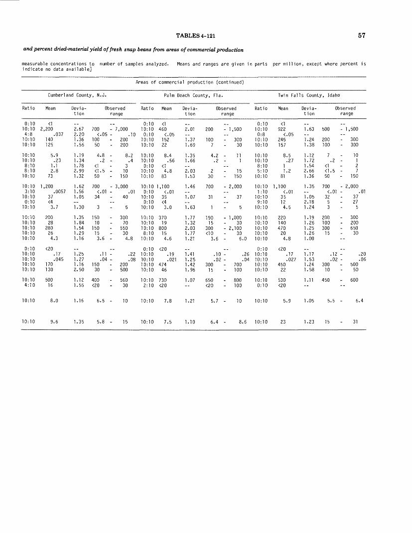
TABLES 4-121
and percent dried-material yield of fresh snap beans from areas of commercial production
57
measurable concentrations to indicate no data available]
number of samples analyzed. Means and ranges are given in parts per million, except where percent is
Areas of commercial production (continued)
10:10
Cumberland County, N.J. Palm Beach County, Fla. Twin Falls County, Idaho
Ratio
0:1010:104:8
10:1010:10
10:1010:108:108:10
10:10
10:103:10
10:100:10
10:10
10:1010:1010:1010:1010:10
0:1010:1010:1010:1010:10
10:104:10
Mean
<12,200
.037140125
5.9.23
1.12.8
73
1,200.0057
37<43.7
20028
280264.3
<20.17.045
170130
50016
Devia tion
__2.672.201.361.56
1.191.341.782.991.32
1.621.561.05—1.30
1.351.841.541.291.16
__1.251.271.162.50
1.121.55
Observed range
700<.05
10050
4.8.2
<1<1.550
700<.01
34
3
15010
150153.6
.11
.04150
30
400<20
_.- 7,000
.10- 200- 200
8.2.4
310
- 150
- 3,000.01
40_-
5
- 30070
- 550304.8
__.22.08
- 200500
- 56030
Ratio
0:1010:100:10
10:1010:10
10:1010:100:10
10:1010:10
10:100:10
10:100:10
10:10
10:1010:1010:108:10
10:10
0:1010:1010:1010:1010:10
10:102:10
Mean
<1460
<.0515222
8.4.56
<14.8
83
1,100<.01
35<43.0
37019
800154.6
<20.19.021
47446
730<20
Devia tion
__2.01__1.371.69
1.351.66__2.031.53
1.46__1.07__1.63
1.771.322.031.771.21
._1.411.251.421.96
1.07--
Observed range
200
1007
4.2.2
230
700
31
1
15015
300<10
3.6
.10
.02300
15
650<20
__- 1,500__- 300
30
111
__15
150
- 2,000__
37__
5
- 1,00030
- 2,100306.0
._.26.04
- 700- 100
- 800100
Ratio
0:1010:100:8
10:1010:10
10:1010:108:105:10
10:10
10:101:10
10:109:10
10:10
10:1010:1010:1010:1010:10
0:1010:1010:1010:1010:10
10:100:10
Mean
<1922
<.05245157
8.5.27
11.2
81
1,100<.01
35124.5
220140470
204.8
<20.17.027
45022
530<20
Devia tion
__1.63__1.241.38
1.121.721.542.661.36
1.35-_1.052.181.24
1.191.261.251.261.00
__1.171.531.241.58
1.11--
Observed range
500
200100
7.2
<1<1.550
700<.01
3253
200100300
15
.12
.02300
10
450
__- 1,500-_- 300- 300
10127
- 150
- 2,000.01
3727
5
- 300- 200- 650
30--
__.20.06
- 50050
- 600--
1.16 6.5 - 10 10:10 1.21 5.7 - 10 10:10 5.9 1.05 5.5 - 6.4
10:10 9.6 1.35 15 10:10 7.5 1.10 6.4 8.6 10:10 23 1.23 15 31
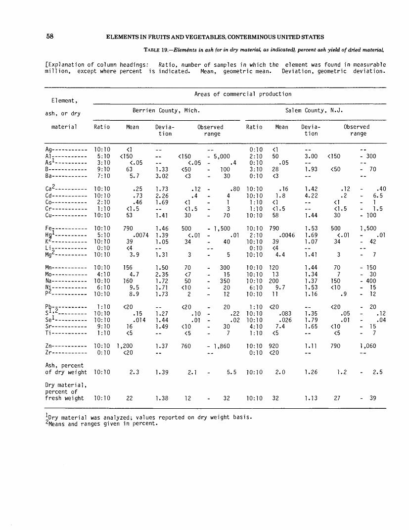
58 ELEMENTS IN FRUITS AND VEGETABLES, CONTERMINOUS UNITED STATES
TABLE 19.—Elements in ash (or in dry material, as indicated), percent ash yield of dried material,
[Explanation of column headings: Ratio, number of samples in which the element was found in measurable million, except where percent is indicated. Mean, geometric mean. Deviation, geometric deviation.
Element,
ash, or dry
material
An-rtg__ —— _ —— ____
A1-------_- -rt i_ -------Ac-1-- _ _
D -%
fa 2p jCo ———————r r _ _ _ _ _____Cu- ----------
Fp_ _ _ _ _____HQ!i/Z
Mg 2 ---------
Mn — — — —Mo— ——————NaNi— — — --p^
Ph.. ————S*> 2--Se 1 — -- —Sr — — — —Ti~— — —
Zn —..—.—Zr — — — —
Ash, percent of dry weight
Dry material , percent of fresh weight
Areas of commercial production
Berrien County, Mich.
Ratio
10:10 5:10 3:10 9:10 7:10
10:10 10:10 2:10 1:10
10:10
10:10 5:10
10:10 0:10
10:10
10:10 4:10
10:10 6:10
10:10
1:10 10:10 10:10 9:10 1:10
10:10 0:10
10:10
10:10
Mean
<1 <150
<.63
5.
<1.53
79039*
<4 3.
156 4.
160 9. 8.
<20
16 <5
1,200 <20
2.
22
05
7
25 73 46 5
0074
9
7
5 9
15 014
3
Devia tion
1.33 3.02
1.73 2.26 1.69
1.41
1.46 1.39 1.05
1.31
1.50 2.35 1.72 1.71 1.73
1.27 1.44 1.49
1.37
1.39
1.38
Observed range
<150 <.05
<50 <3
.12
.4 <1 <1.5 30
500 <.01
34
3
70 <7 50
<10 2
<20 .10 .01
<10 <5
760
2.1
12
- 5,000 .4
100 30
.80 4 1 3
70
- 1,500 .01
40
5
- 300 15
- 350 20 12
20 .22 .02
30 7
- 1,860
5.5
32
Ratio
0:10 2:10 0:10 3:10 0:10
10:10 10:10 1:10 1:10
10:10
10:10 2:10
10:10 0:10
10:10
10:10 10:10 10:10 6:10
10:10
1:10 10:10 10:10 4:10 1:10
10:10 0:10
10:10
10:10
Salem County
Mean
<1 50
.05 28 <3
.16 1.8
<1 <1.5 58
790 .0046
39 <4 4.4
120 13
200 9.7
11
<20 .083 .026
7.4 <5
920 <20
2.0
32
Devia tion
3.00
1.93
1.42 4.22
1.44
1.53 1.69 1.07
1.41
1.44 1.34 1.37 1.53 1.16
1.35 1.79 1.65
1.11
1.26
1.13
, N.J.
Observed range
<150
<50
.12
.2 <1 <1.5 30
500 <.01
34
3
70 7
150 <10
.9
<20 .05 .01
<10 <5
790
1.2
27
- 300
- 70
.40 - 6.5 - 1 - 1.5 - 100
1,500 .01
- 42
- 7
- 150 - 30 - 400 - 15 - 12
- 20 .12 .04
- 15 - 7
1,060
- 2.5
- 39
material was analyzed; values reported on dry weight basis. 2Means and ranges given in percent.
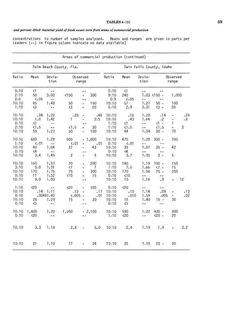
TABLES 4-121
and percent dried- material yield of fresh sweet corn from areas of commercial production
concentrations to number of samples analyzed. Means and ranges are given in parts per Leaders (--) in figure column indicate no data available]
59
Areas of commercial production (continued)
Palm Beach County, Fla.
Ratio
0:102:100:8
10:101:10
10:1010:100:102:10
10:10
10:101:10
10:100:10
10:10
10:103:10
10:108:10
10:10
1:1010:108:10
10:100:10
10:100:10
Mean Devia tion
<150 3<.05
85 1<3
.34 11.8 1
<1<1 .559 1
680 1<.01
40 1<43.4 1
160 15.0 1
170 111 19.0 1
<20.14 1.00481
26 1<5
1,400 1<20
__.00--
.48--
.20
.42----
.27
.29__
.04__
.45
.37
.31
.75
.32
.00
_ _
.11
.40.29"--
.20--
Observed range
<150
50<3
.281
<1.550
500<.01
37
2
70<775
<10
<20.13
<.00515
1,050
__- 300--- 150
20
.462.5
--30
- 100
- 1,000.01
43__
5
- 2007
- 30015
--
100.17.01
30--
- 2,100--
Ratio
0:9:
010:
5:
10:10:
1:1:
10:
10:0:
10:0:
10:
10:7:
10:0:
10:
0:10:10:10:0:
10:1:
1010:91010
1010101010
1010101010
1010101010
1010101010
1010
Twin Falls County, Idaho
Mean Devia tion
<1240
<.572.
.<1<1 .44
470<.
39<43.
1407.
170<1010
<20..
18<5
590<20
05
9
1843
5
01
7
5
i
10010
__
1.83--1.273.31
1.201.64----1.34
1.29_-1.07__1.30
1.191.661.56--1.16
_ _1.141.591.40--
1.22--
Observed range
__<150 -
--50 -<3 -
.14
.2<1 -<1 .530 -
300 -__
35 -__
3 -
100 -<7 -75 -
--.9
— —
.09
.00515 -
--
420 -<20 -
1,000
10020
.26
.81
370
700
42
5
15015350
- 12
.13
.0230
80020
10:10 3.3 1.18 5.0 10:10 2.4 1.19 1.9 3.2
10:10 21 1.10 17 24 10:10 25 1.10 23 - 30
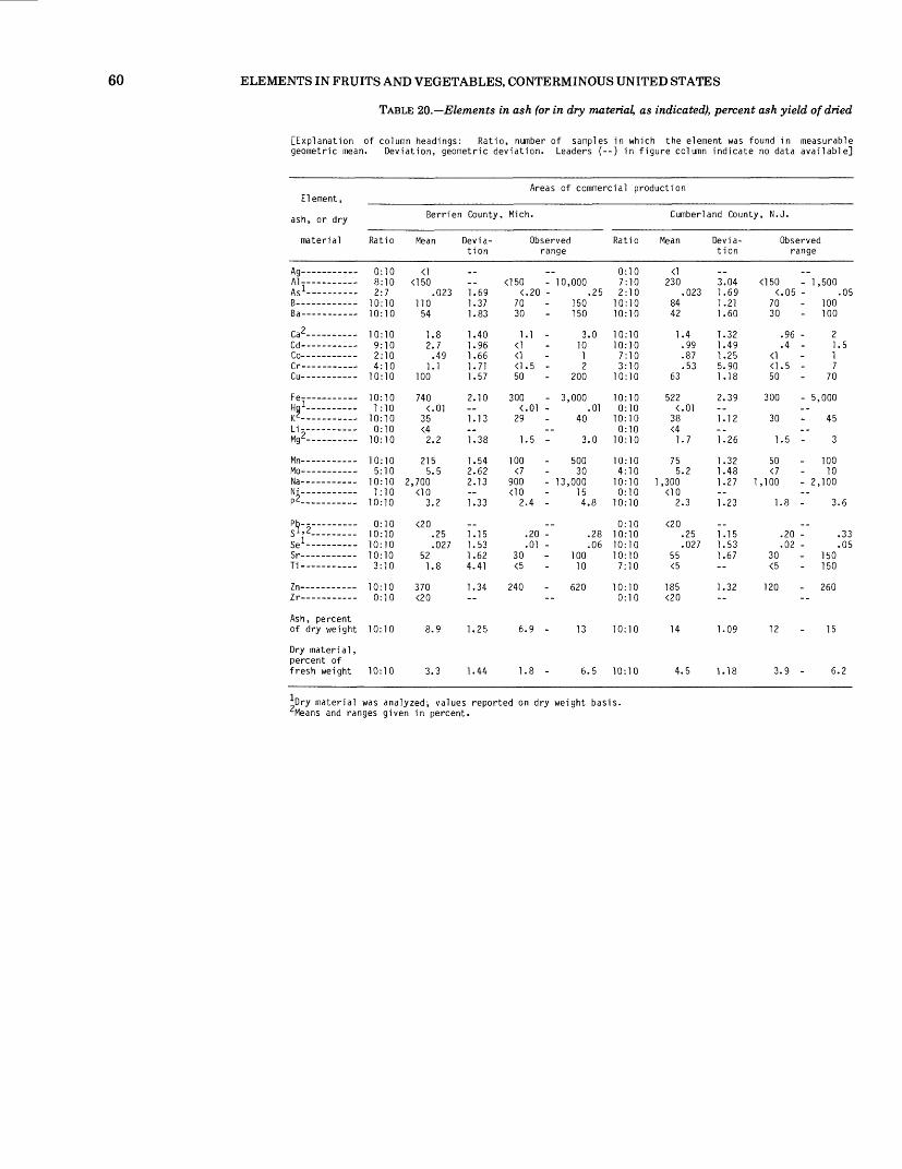
60 ELEMENTS IN FRUITS AND VEGETABLES, CONTERMINOUS UNITED STATES
TABLE 20.—Elements in ash (or in dry material, as indicated), percent ash yield of dried
[Explanation of column headings: Ratio, number of samples in which the element was found in measurable geometric mean. Deviation, geometric deviation. Leaders (--) in figure column indicate no data available]
Element,
ash, or dry
Areas of commercial production
Berrien County, Mich. Cumberland County, N.J.
material
AV— — -Ac -
D •}
Pa 2
Co —————— .rvC U —————— .
Fe ______ .iH n i
L/Z
9Mg^ —————— .
Mn ——— - —— .Mo ——————— •Na —————— -Mi
P
ph —————————— .sl. 2LI-:::::::::Qi«
Pi- _______ .
Ratio
- 0:108 . i ri
- 2:7- 10:10- 10:10
- 10:10- 9:10- 2:10- 4:10- 10:10
- 10:10- 1:10- 10:10- 0:10- 10:10
- 10:10- 5:10- 10:10- 1:10- 10:10
- 0:10- 10:10- 10:10- 10:10
T-in
Mean
<1<150
.023110
54
1 02.7
.491.1
100
740<.01
35<42.2
5.52,700
<103.2
<20.25.027
52i «
Devia tion
1.691.371 00
1.401.961.661.711.57
2.10
1.13
1 T Q
1.542.622.13
1.33
1.15
1 £O
d dl
<150<
7030
1<1<1<150
300<
29
1
100<7
900<10
2
30<-R
Observed range
- 10, .20 -
.1 -
.5 -
- 3,.01 -
.5 -
- 13,
.4 -
.20 -
.01 -
00025
150150
1012
200
000.01
40
3.0
50030
000154 Q
OQ
.06100in
Ratio
0:107:102:10
10:1010:10
10:1010:107:103:10
10:10
10:100:10
10:100:10
10:10
10:104:10
10:100:10
10:10
0:1010:1010:1010:107-in
Mean
<1230
.0238442
1.4.9907
63
522<.01
OQ
<41.7
755.2
1,300 <10
<20.25.027
55<•<;
Devia tion
3.041.691.211.60
1.321.49
1 1 Q
2.39
1.12
1 r\ r
1.321.481.27
1.23
1.151.531.67
Observed range
<150 - 1,<.05 -
7030
.96 -
.4 -<1<1.5 -50
300 - 5,
30
1.5 -
50<7
1,100 - 2,
1 0
.20 -
.02 -30<-<;
500.05
100100
21.517
70
000
3
10010
100
O r
.33
.05150i<;n
Zr ——————— 0:10 <20
Ash, percent of dry weight 10:10 8.9 1.25 6.9 -
Dry material , percent of fresh weight 10:10 3.3 1.44 1.8 -
*Dry material was analyzed; values reported on dry Means and ranges given in percent.
13
6.
weight
0:10
10:10
,5 10:10
basis.
<20
14 1.09 12 - 15
4.5 1.18 3.9 - 6.2

TABLES 4-121
material, and percent dried-material yield of fresh tomatoes from areas of commercial production
61
concentrations to number of samples analyzed. Means and ranges are given in parts per million, except where percent is indicated. Mean,
Areas of commercial production (continued)
Palm Beach County, Fla.
Ratio
D:106:101:79:100:10
10:109:101:103:10
10:10
10:101:10
10:100:10
10:10
10:109:10
10:100:10
10:10
0:1010:109:10
10:100:10
10:100:10
Mean
<i153
<.0565<3
.70
.38<1
.81121
380<.01
30<4
1.3
737.5
3,200<10
1.6
<20.19.015
55<5
210<20
Devia tion
..2.28--1.47—
1.622.46—2.331.47
1.46--1.20--1.35
1.381.351.28—1.33
__1.082.712.00--
1.34--
Observed range
_.<150 - 200
<.05 - .05<50 - 150
—
.82 - 1.5<.2 - 1.5
<1 - 1<1.5 - 370 - 200
300 - 700<.01 - .01
23 - 42--
.7 - 2
50 - 150<7 - 15
2,500 - 5,900--
1.2 - 2.4
__.18 - .23.01 - .02
30 - 150--
160 - 350--
Ratio
0:105:101:8
10:1010:10
10:1010:105:103:10
10:10
10:101:10
10:100:10
10:10
10:102:10
10:. 109:10
10:10
0:1010:1010:1010:105:10
10:100:10
Yakiman County
Mean
<!133
<.l 58113
1.02.2.74.91
73
550<.01
34<41.6
1141.7
3,600152.5
<20.21.035
924
250<20
Devia tion
__2.86--1.361.76
1.991.841.391.871.22
1.65.-1.24--1.25
1.374.121.441.461.38
_.1.202.442.142.32
1.45--
, Wash.
Observed range
_.<150
<.05 -50
5
.80 -1
<1<1 . 5 -50
500 - 1,<.01 -
23--
1.5 -
70<7
2,300 - 6,<10
1.2 -
...14 -.10 -
30<5
110--
San Joaquin County, Calif.
700.15
15030
3.25.512
100
000.01
45
2
15020
800303.6
.26
.15300
15
400
Ratio
D:104:102:10
10:1010:10
10:1010:101:100:10
10:10
10:102:10
10:100:10
10:10
10:1010:1010:100:10
10:10
0:1010:1010:1010:100:10
10:100:10
Mean
<•)
92<.023
8140
1.2.38
<1<1 .537
300.0046
31<4
1.6
8816
11,000<10
2.5
<20.16.16
280<5
130<20
Devia tion
__3.311.691.201.65
1.301.90----1.30
1.241.691.10--1.15
1.431.381.77--1.24
__1.131.781.32--
1.57--
<150<.
7020
<1
30
200<.
27
1.
5010
4,000
1.
200
80
Observed range
..700
05 - .05100
70
82 - 1.82 - 1.0
4--
50
50001 - .01
36--
5 - 2
15030
- 26,000--
8 - 3.6
__14 - .2108 - .35
500--
240--
10:10 14 9.1 10:10 13 10:10 1.20 13
10:10 5.2 1.27 3.0 - 6.9 10:10 6.4 1.18 5.4 - 8.9 10:10 7.6 1.05 7.0
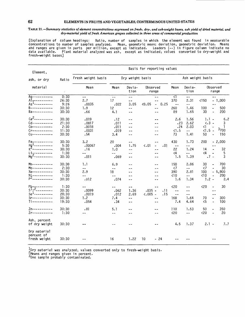
62 ELEMENTS IN FRUITS AND VEGETABLES, CONTERMINOUS UNITED STATES
TABLE 21.—Summary statistics of element concentrations expressed on fresh-, dry-, and ash-weight bases, ash yield of dried material, and dry-material yield of fresh American grapes collected in three areas of commercial production
[Explanation of column headings: Ratio, number of samples in which the element was found in measurable concentrations to number of samples analyzed. Mean, geometric mean; deviation, geometric deviation. Means and ranges are given in parts per million, except as indicated. Leaders (--) in figure column indicate no data available. Plant material analyzed was ash, except as indicated; values converted to dry-weight and fresh-weight bases]
Element,
ash, or dry
material
An--- -___--tty----------- ni _ ________Ml- ——————— -Ac-1- __ _ _ ___ _
D-»
fa 2f* jCd- — — -----Co —— — ——r>_ _ _______Cu — -- ——— -
Fe-- ____ --i Hg 1 ———————KzLi-— ... ... _Mg^ __________
Mn — — _-_ — _Mo -—__——MANi— — — ~p2___________
Ph_ _______Sl» 2— — ~Se 1— — — -Qr _ _________
Ti- —————— -
Zn — - ————"7 M
Ash, percent of dry weight
Dry material percent of fresh weight
Basis for reporting values
Ratio |rresn weight basis Dry weight basis Ash weight basis
0:30 26:30 9:26
30:30 30:30
30:30 21:30 2:30
11:30 30:30
30:30 5:30
30:30 1:30
30:30
30:30 2:30
30:30 1:30
30:30
1:30 30:30 28:30 30:30 19:30
30:30 1:30
30:30
30:30
Mean
2.7 .0035
1.9 .66
.019
.0017
.0018
.0031
.54
3.2 .00067 .16
.011
1.1
2.9
.012
.0099
.0019 1.2 .054
.81
Mean
17 .022
12 4.1
.12
.011
.011
.019 3.4
20 .004
1.0
.069
6.9
18
.074
.062
.012 7.4 .34
5.1
16
Devia- Observed Mean tion range
<1370
3.05 <0.05 - 0.25 260 89
2.6 .23 .24
<1.5 73
430 1.75 <.01 - .01
22 <4 1.5
150 <7
390 <10
1.6
<20 1.36 .035 - .11 2.69 <.005 - .15
160 7.4
110 <20
4.5
1.22 10 - 24
Devia tion
2.31
1.46 1.65
1.56 2.62 2.03
1.41
1.73
1.24
1.39
2.86
2.81
1.34
1.64 4.64
1.53
1.37
<150
100 30
1 <
<1 <150
200
14 <4
30 <7
100 <10
1
<20
70 <5
50 <20
2
Observed range
- 1,000
- 500 - 200
.1 - 6.2
.3 - 3
.5 - 3700 - 150
- 2,000
32 5
.7 - 3
- 700 30
- 5,900 - 200
.2 - 2.4
30
- 300 - 100
- 350 20
.1 - 7.7
^Dry material was analyzed; values converted only to fresh-weight basis. ^Means and ranges given in percent. '•'One sample probably contaminated.

TABLES 4-121 63
TABLE 22.—Summary statistics of element concentrations expressed on fresh-, dry-, and ash-weight bases, ash yield of dried material, and dry-material yield of fresh apples collected in five areas of commercial production
[Explanation of column headings: Ratio, number of samples in which the element was found in measurable concentrations to number of samples analyzed. Mean, geometric mean; deviation, geometric deviation. Means and ranges are given in parts per million, except as indicated. Leaders (—) in figure column indicate no data available. Plant material analyzed was ash, except as indicated; values converted to dry-weight and fresh-weight bases]
Element,
ash, or dry
material
An-----_---_-My___________
Al-----------ttl Ac 1 -- _ _ _ ___
D i
rv.2rd_ _ _ ______Co ———————o_ _ ________Cu ———— ———
Fe ———————Hn 1 Hg ————————i/£LT- —— .... ——Mg^ ——— - ————
Mn ——— - ———Mo ———————Na ———————Ni ———————p2___________
Pb ———————Sl> 2— — —se i— — — -oc
Ti ———————
Zn ———————7 «
Ash, percent of dry weight
Dry material, percent of fresh weight
Basis for reporting values
Ratio
1:50 45:50 37:48 50:50 50:50
50:50 36:50 10:50 15:50 50:50
50:50 13:50 50:50 1:50
50:50
50:50 14:50 50:50
1:50 50:50
14:50 50:50 25:50 50:50 38:50
50:50 0:50
50:50
50:50
Fresh weight basis
Mean
1.1 .20
1.2 .21
.0030
.0051
.0012
.0019
.17
.92
.094
.0040
.20
.011 1.6
.0059
.0073
.0039
.00039
.26
.027
.18
Dry weight basis
Mean Devia- Observed tion range
7.2 <.05 — <.05 - 10 8.3 1.4
.020
.034
.0083
.013 1.1
6.1 <.01 — <.01 - .12
.63
.027
1.3 .070
11
.040
.049
.026 1.35 .015 - .045
.0026 3.36 <.005 - .08 1.7
.18
1.2
14 1.09 10 - 19
Mean
<1400
455 77
1.1 .19 .46 .70
63
350
35 <4 1.5
74 3.9
600 <10
2.2
2.7
97 10
67 <20
1.6
Ash weight
Devia tion
2.34
1.52 1.81
1.56 1.76 1.69 2.98 1.33
1.41
1.21
1.29
1.94 1.92 2.03
1.23
2.71
2.19 2.92
1.47
1.24
basis
<1 <150
150 20
< <1 <1 30
200
17 <4
20 <7
100 <10
1
<20
15 <5
35
1
Observed range
2 - 3,000
- 1,500 - 200
.48- 3.2
.2 - .6 1
.5 - 7 100
- 1,000
43 4
.7 - 2
- 200 10
- 3,100 15
.2 - 3.6
- 1,000
- 300 70
190
.1 - 4.3
Dry material was analyzed; values converted only to fresh-weight basis. Means and ranges given in percent.
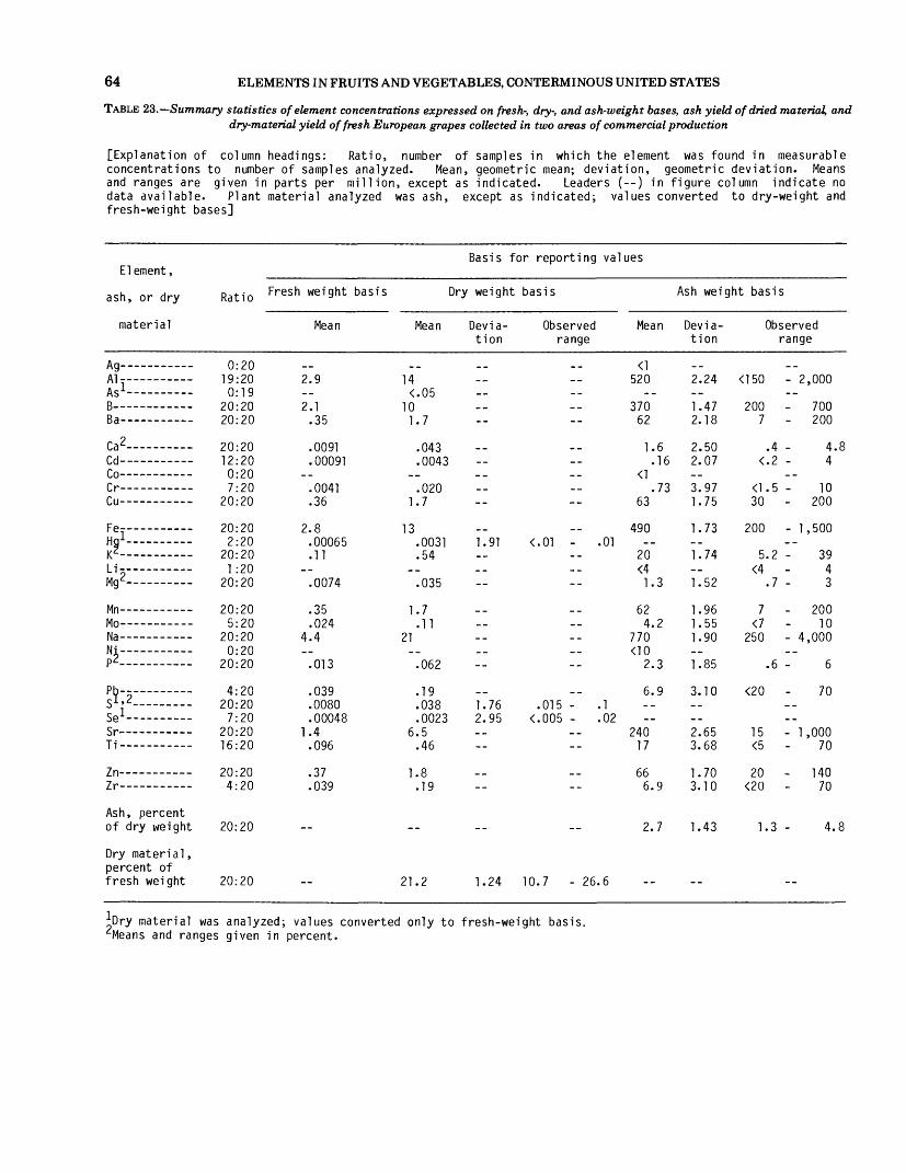
64 ELEMENTS IN FRUITS AND VEGETABLES, CONTERMINOUS UNITED STATES
TABLE 23.—Summary statistics of element concentrations expressed on fresh-, dry-, and ash-weight bases, ash yield of dried material, and dry-material yield of fresh European grapes collected in two areas of commercial production
[Explanation of column headings: Ratio, number of samples in which the element was found in measurable concentrations to number of samples analyzed. Mean, geometric mean; deviation, geometric deviation. Means and ranges are given in parts per million, except as indicated. Leaders (--) in figure column indicate no data available. Plant material analyzed was ash, except as indicated; values converted to dry-weight and fresh-weight bases]
Element,
ash, or dry
material
An-----------M y
Ai _ _ _______HIAc 1 -- __ _____r\o
R-,_ ___
r,2f* A
Co ———————(Y---------Cu —————— -
FP ———————Hnl
K^_____1 !___________LIMg^ ————— - ——
Mn ——— _ ——Mo— ——— --N-,Ni-— — —p
Pb-- ————cl,2Se 1 — — -"-"$r — _ _ _ _Ti-----__--__
7n-----------7,_
Ash, percent of dry weight
Dry material, percent of fresh weight
Basis for reporting values
Ratio Fresl1 wei ght basis Dry weight basis
0:20 19:20 0:19
20:20 20:20
20:20 12:20 0:20 7:20
20:20
20:20 2:20
20:20 1:20
20:20
20:20 5:20
20:20 0:20
20:20
4:20 20:20
7:20 20:20 16:20
20:20 4:20
20:20
20:20
Mean
2.9
2.1.35
.0091
.00091
.0041
.36
2.8 .00065 .11
.0074
.35
.024 4.4
.013
.039
.0080
.00048 1.4
.096
.37
.039
Mean
14 <.05
10 1.7
.043
.0043
.020 1.7
13 .0031 .54
.035
1.7 .11
21
.062
.19
.038
.0023 6.5
.46
1.8 .19
21.2
Devia- Observed Mean tion range
<1 520
370 62
1.6 .16
<1 .73
63
490 1.91 <.01 - .01
20 <4 1.3
62 4.2
770 <10
2.3
6.9 1.76 .015 - .1 2.95 <.005 - .02
240 17
66 6.9
2.7
1.24 10.7 - 26.6
Ash weight basis
Devia tion
2.24
1.47 2.18
2.50 2.07
3.97 1.75
1.73
1.74
1.52
1.96 1.55 1.90
1.85
3.10
2.65 3.68
1.70 3.10
1.43
<150
200 7
<
<130
200
5 <4
7 <7
250
<20
15 <5
20 <20
1
Observed range
- 2,000
- 700 - 200
.4 - 4.8
.2 - 4
.5 - 10 - 200
- 1,500
.2 - 39 4
.7 - 3
- 200 10
- 4,000
.6 - 6
70
- 1,000 70
- 140 70
.3 - 4.8
*Dry material was analyzed; values converted only to fresh-weight basis. ^Means and ranges given in percent.

TABLES 4-121 65
TABLE 24.—Summary statistics of element concentrations expressed on fresh-, dry-, and ash-weight bases, ash yield of dried material, and dry-material yield of fresh grapefruit collected in four areas of commercial production
[Explanation of column headings: Ratio, number of samples in which the element was found in measurable concentrations to number of samples analyzed. Mean, geometric mean; deviation, geometric deviation. Means and ranges are given in parts per million, except as indicated. Leaders (--) in figure column indicate no data available. Plant material analyzed was ash, except as indicated; values converted to dry-weight and fresh- weight bases]
Element,
ash, or dry
material
fl a _ _A!. _ _ _ _ _Ml- ————————— -
Ac 1 - _______
Ra
Ca 2TH_ _ _ _ _ __fn _ _ __ _ _ _fr_Cu ——————————
Fe ——————Hnl Hg ———————yi
Li .......Mȣ
Mm
MA
MaNi— ..... —p2_....___ —
Ph__ —————S*j2-~~So 1 - ______cr_ ___ __ _ _Ti ———————
Z n ———————2r- —————
Ash, percent of dry weight
Dry material, percent of fresh weight
Basis for reporting values
Ratio f:resh weight basis Dry weight basis
0:4 33:40 17:36 40:40 40:40
40:40 23:40 4:40 8:40
40:40
40:40 0:40
40:40 22:40 40:40
40:40 3:40
40:40 5:40
40:40
1:40 40:40 32:40 40:40 22:40
40:40 0:40
40:40
40:40
J,Dry material was analyzed Means and ranges given in
Mean
1.4 .0034 .65 .29
.022
.00061
.00068
.0018
.19
1.2
.14
.014
.0072
.13
.012 6.1
.065
.011
.0066
.0010 2.5
.021
.49
Mean Devia- Observed tion range
14 .034 2.93 <.05 - .4
6.5 2.9
.22
.0061
.0068
.018 1.9
12 <.01 1.4
.14
.072
1.3 .12
61 .65 .11
.066 1.42 <.050 - .095
.010 2.52 <.005 - .06 25
.21
4.9
10 1.20 7.0 - 15
Mean
<1 380
170 77
5.9 .16 .18 .47
50
310
36 3.7 1.9
34 3.1
1,600 17 3.0
<20
650 5.4
130 <20
3.8
Ash weight basis
Devia tion
3.06
1.35 2.04
1.59 1.76 2.87 3.14 1.39
1.82
1.24 2.76 1.46
1.56 1.53 1.57 2.24 1.40
2.22 4.08
1.34
1.43
<150
100 20
1 <
<1 <130
150
15 <4
15 <7
600 10
1
<20
150 <5
60
2
Observed range
- 3,000
- 300 - 200
.2 - 10
.2 - .6 2
.5 - 3 70
- 2,000
42 21
.7 - 3
70 7
- 3,000 70
.2 - 4.8
70
- 2,000 70
- 200
.3 - 11
; values converted only to fresh-weight basis, percent.
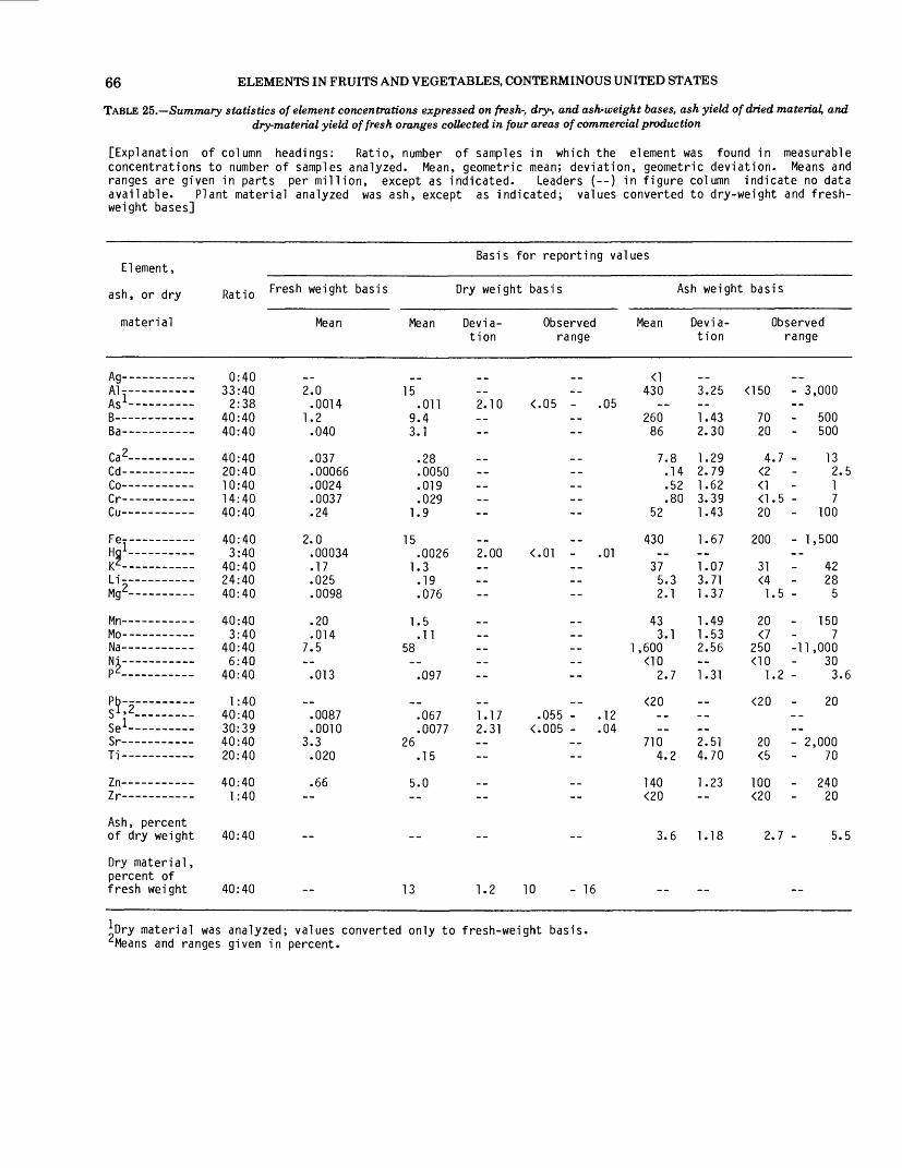
66 ELEMENTS IN FRUITS AND VEGETABLES, CONTERMINOUS UNITED STATES
TABLE 25.—Summary statistics of element concentrations expressed on fresh-, dry-, and ash-weight bases, ash yield of dried material, and dry-material yield of fresh oranges collected in four areas of commercial production
[Explanation of column headings: Ratio, number of samples in which the element was found in measurable concentrations to number of samples analyzed. Mean, geometric mean; deviation, geometric deviation. Means and ranges are given in parts per million, except as indicated. Leaders (--) in figure column indicate no data available. Plant material analyzed was ash, except as indicated; values converted to dry-weight and fresh- weight bases]
Element,
ash, or dry
material
Al-----------Ml - —————— -Ac 1 -- _ ______
D ̂
fa 2r* A
Co ———————r r _ _ ____Cu ———————
Fe —— ___ -i Hn i
Li-——- —ui^c.
M«
Mo —_——___MaN£——— ______
cl>2Se 1— — — -
Ti ___________
Zn _—_—___Zr — — — __
Ash, percent of dry weight
Dry material, percent of fresh weight
Basis for reporting values
Ratio
0:40 33:40 2:38
40:40 40:40
40:40 20:40 10:40 14:40 40:40
40:40 3:40
40:40 24:40 40:40
40:40 3:40
40:40 6:40
40:40
1:40 40:40 30:39 40:40 20:40
40:40 1:40
40:40
40:40
Fresh weight basis
Mean
2.0 .0014
1.2 .040
.037
.00066
.0024
.0037
.24
2.0 .00034 .17 .025 .0098
.20
.014 7.5
.013
.0087
.0010 3.3 .020
.66
Dry weight basis
Mean Devia- Observed tion range
15 .011 2.10 <.05 - .05
9.4 3.1
.28
.0050
.019
.029 1.9
15 .0026 2.00 <.01 - .01
1.3 .19 .076
1.5 .11
58
.097
.067 1.17 .055 - .12
.0077 2.31 <.005 - .04 26
.15
5.0
13 1.2 10 - 16
Mean
430
260 86
7.
52
430
37 5. 2.
43 3.
1,600
2.
<20
710 4.
140 <20
3.
Ash weight
Devia tion
3.25
1.43 2.30
8 1.29 14 2.79 52 1.62 80 3.39
1.43
1.67
1.07 3 3.71 1 1.37
1.49 1 1.53
2.56
7 1.31
2.51 2 4.70
1.23
6 1.18
basis
Observed range
<150
70 20
4.7 <2
20
200
31 <4 1.5
20 <7
250
1.2
<20
20 <5
100 <20
2.7
- 3,000
- 500 - 500
13 2.5 1 7
- 100
- 1,500
42 28 5
150 7
-11,000 30 3.6
20
- 2,000 70
- 240 20
5.5
^Dry material was analyzed; values converted only to fresh-weight basis, and ranges given in percent.

TABLES 4-121 67
TABLE 26.—Summary statistics of element concentrations expressed on fresh-, dry-, and ash-weight bases, ash yield of dried material, and dry-material yield of fresh peaches collected in four areas of commercial production
[Explanation of column headings: Ratio, number of samples in which the element was found in measurable concentrations to number of samples analyzed. Mean, geometric mean ; deviation, geometric deviation. Means and ranges are given in parts per million, except as indicated. Leaders (--) in figure column indicate no data available. Plant material analyzed was ash, except as indicated; values converted to dry-weight and fresh- weight bases]
Element,
ash, or dry
material
A?A 1
D •*
Ca 2PICo ---------fV_ _ _ _C U ———— -----
FP — — ___ -i Hg 1 — —————
Li- ———— ——
Mn ———————Mo ———————MaNi ———————
Ph ———————
Li— -sr_ _ _______Ti— — — —
Zn ——————Zr ———————
Ash, percent of dry weight
Dry material , percent of fresh weight
Basis for reporting values
Ratio
2:40 33:40 15:37 40:40 37:40
40:40 24:40 8:40
20:40 40:40
40:40 7:40
40:40 1:40
40:40
40:40 1:40
40:40 18:40 40:40
2:40 40:40 23:40 40:40 24:40
40:40 3:40
40:40
40:40
Fresh weight basis
Mean
.00058 2.6
.0026 2.3
.11
.0017
.0011
.0018
.0078
.34
1.8 .00034 .11
.0066
.25
.96
.044
.0090
.072
.0043
.00046
.28
.55
.025
Dry weight basis
Mean Devia- Observed tion range
.0059 26
.026 4.26 <.05 - .35 23
1.1
.017
.011
.018
.078 3.4
18 .0034 2.17 <.01 - .02
1.1
.066
2.5
9.6 .44 .090
.72
.043 1.57 .020 - .12
.0046 2.57 <.005 - .02 2.8
5.5 .25
10 1.47 3.6 - 17
Ash weight basis
Mean
.098 430
380 18
.29
.19
.30 1.3
56
300
19 <4
1.1
42 <7
160 7.3 1.5
12
46 <5
91 4.2
6.7
Devia tion
3.65 3.35
1.55 2.94
1.85 3.69 2.73 3.41 1.80
2.31
1.52
1.47
1.98
1.79 2.65 1.76
1.28
2.02
1.78 2.76
1.60
Observed range
<150 - 7,
150 - 1, <3
.12 -
20
70 - 2,
8.5 - <4
.5 -
15 <7 50
.32 -
<20
15 <5
30 <20
1.5 -
2 000
000 200
1.2 3 2
15 200
000
43 4 3
150 7
450 70 4.8
20
300 30
300 30
15
k)ry material was analyzed; values converted only to fresh-weight basis. ^Means and ranges given in percent.

68 ELEMENTS IN FRUITS AND VEGETABLES, CONTERMINOUS UNITED STATES
TABLE 27.—Summary statistics of element concentrations expressed on fresh-, dry-, and ash-weight bases, ash yield of dried material, and dry-material yield of fresh pears collected in five areas of commercial production
[Explanation of column headings: Ratio, number of samples in which the element was found in measurable concentrations to number of samples analyzed. Mean, geometric mean; deviation, geometric deviation. Means and ranges are given in parts per million, except as indicated. Leaders (—) in figure column indicate no data available. Plant material analyzed was ash, except as indicated; values converted to dry-weight and fresh-weight bases]
Element,
ash, or dry
material
An-- --AI_iAs-1 ------- --
Ra
r,2PH. _ ________Co-— ———rr___ _ ______Cu ———————
Fe-—- — —Hg 1 ———————V?--- _ _______Li ————— —Mg^ —————————
Mn-------- _ -Mo ————————NA|\|i ___ __ __9p2 ————————
Rh ————————$1' 2— — —Se1 - —$r _____ _Ti ___________
ZnZr-----------
Ash, percent of dry weight
Dry material , percent of fresh weight
Basis for reporting values
Ratio frresn we ight basis Dry weight basis Ash weight basis
0:50 42:50 9:50
50:50 50:50
50:50 38:50 30:50 19:50 50:50
50:50 7:50
50:50 11:50 50:50
50:50 8:50
50:50 17:50 50:50
7:50 50:50 35:50 50:50 26:50
50:50 3:50
50:50
50:50
Mean
1.1
1.4 .47
.0057
.00085
.0028
.022
.35
.91
.00057
.072
.0035
.0047
.26
.0060 1.8 .018 .0050
.031
.0044
.00087
.57
.47
.022
Mean
7.1 <.05 9.2 3.2
.038
.0057
.019
.014 2.3
6.1 .0038 .48 .023 .032
1.7 .040
12 .12 .034
.21
.029
.0058 3.8
3.2 .15
15
Devia- Observed Mean tion range
<1340
<.05 - .55 440 150
1.8 .27 .90 .69
110
290 1.80 <.01 - .01
23 1.1 1.5
83 1.9
560 5.7 1.6
9.8 1.32 .015 - .05 2.31 <.005 - .02
180 <5
150 7.1
2.1
1.17 11 - 20
Devia tion
2.93
1.53 1.86
1.76 2.55 2.64 5.47 1.69
1.76
1.41 3.71 1.35
1.65 3.07 2.50 2.37 1.63
1.74
2.04
2.01 1.81
1.33
<150
150 30
<<1 <130
70
10 <4
20 <7
150 <10
<20
30 <5
10 <20
1
Observed range
- 7,000
- 1,000 - 700
.52- 5.4
.2 - 3 10
.5 - 100 - 300
- 1,000
42 17
.7 - 3
150 20
- 6,600 70
.6 - 3.6
30
- 700 - 200
- 720 30
.0 - 3.7
Dry material was analyzed; values converted only to fresh-weight basis. Means and ranges given in percent.

TABLES 4-121 69
TABLE 28.—Summary statistics of element concentrations expressed on fresh-, dry-, and ash-weight bases, ash yield of dried material, and dry-material yield of fresh plums collected in four areas of commercial production
[Explanation of column headings: Ratio, number of samples in which the element was found in measurable concentrations to number of samples analyzed. Mean, geometric mean; deviation, geometric deviation. Means and ranges are given in parts per million, except as indicated. Leaders (--) in figure column indicate no data available. Plant material analyzed was ash, except as indicated; values converted to dry-weight and fresh-weight bases]
Element,
ash, or dry
material
fl a _ _ _ _ _____My___________
Al__ _ _HI-- flc 1 - ____ __ __
D 3
Ca 2/* j
Co ———————Cr-----------Cu ----------
Fe--— — —Ha 1 — — — ——K ZLi-- — ______Mg^ — ——— —
Mn ——— ———Mo ———————M,
Ni— ________p2___________
Pb ——— ————s"> 2—Li —— —— — -Sr ---------T-j_ _ ________
Zn ——— _____Zr ——— — —
Ash, percent of dry weight
Dry material , percent of fresh weight
Ratio
4:4028:40
40:4040:40
40:4016:402:40
11:4040:40
40:405-40
40:400:40
40:40
40:408:40
40:403-40
40:40
10:4040:4029:4040:4016:40
40:401:40
40:40
40:40
Fresh weight basis
Mean
1.4
2.5.22
nmo..00081
.0044
1.4.00049.11
.0074
.36
.025Q1
.033
.0074
.056
.0045
.00080
.60
1.7
--
Mean
10<.05
1 Q
1 • *J
.027
.0058
03?2.4
10.0035.77
.053
1 P.
5 0
.24
.40
.032
.0057T^ • J
12
14
Basis for reporting values
Dry weight basis
Devia- Observed Mean tion range
<1210
<.05 - 3
32
.12<1
.6651
2001.84 <.010 - .010
.6<4
1.1
5337
1204.91.1
8.41.31 .020 - .0552.08 <.0050 - .020
<5
120<20
4.8
1.29 8.0 - 20
Ash weight
Devia tion
2.43 <
1.592 93
i . ~ j1 O C
2 on
2.01
1.72
1 . J T^
1 07
1 651.671.451 7P,
3 1 2
1 • J <J
2.12
1.44
basis
Observed range
<1150 - 1,
150 - 1,7 - 1,
<.2 -<1<1 5 -15
50
9
10<7<7
<10.6 -
<20
15<5
30<20
2.2 -
3500
500500
1.2.4
27
200
500
oc
2.0
1501010102.4
70
300150
77020
17
j;Dry material was analyzed; values converted only to fresh-weight basis. ^Means and ranges given in percent.
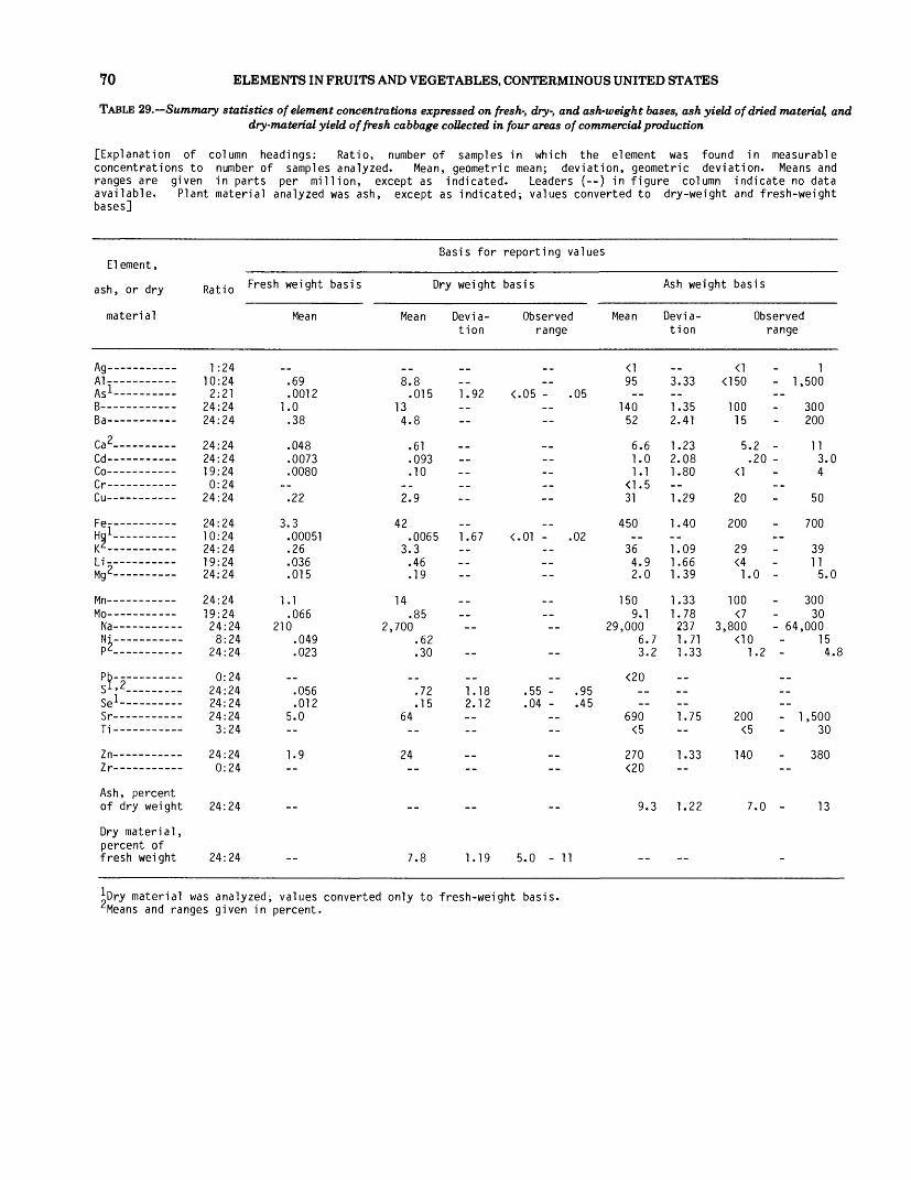
70 ELEMENTS IN FRUITS AND VEGETABLES, CONTERMINOUS UNITED STATES
TABLE 29.—Summary statistics of element concentrations expressed on fresh-, dry-, and ash-weight bases, ash yield of dried material, and dry-material yield of fresh cabbage collected in four areas of commercial production
[Explanation of column headings: Ratio, number of samples in which the element was found in measurable concentrations to number of samples analyzed. Mean, geometric mean; deviation, geometric deviation. Means and ranges are given in parts per million, except as indicated. Leaders (--) in figure column indicate no data available. Plant material analyzed was ash, except as indicated; values converted to dry-weight and fresh-weight bases]
Element,
ash, or dry
material
Ratio f?res '1 weight basis
Mean
Basis for reporting values
Dry weight basis Ash weight basis
Mean Devia tion
Observed range
Mean Devia tion
Observed range
Ag——————— 1:24Al-—————— 10:24 .69As 1 —————— - 2:21 .0012B———————— 24:24 1.0Ba——————- 24:24 .38
Ca 2—-———— 24:24 .048Cd——————— 24:24 .0073Co———--—— 19:24 .0080C r—- —— -— 0:24Cu————-—— 24:24 .22
Fe- —------ 24:24 3.3Hg 1—-———— 10:24 .00051Kz——————— 24:24 .26Li-—————— 19:24 .036Mg^—————— 24:24 .015
Mn——————— 24:24 1.1Mo——————— 19:24 .066Na—- ——-- 24:24 210Ni——————— 8:24 .049p^——————— 24:24 .023
Pb- 5—------ 0:24S 1 ^— ----- 24:24 .056Se 1—————— 24:24 .012Sr--- ———— -- 24:24 5.0Ti— ——— -— 3:24
In-- — — — -- 24:24 1.9Zr—- —— — 0:24
Ash, percent of dry weight
Dry material, percent of fresh weight
24:24
24:24
.015134.8
.61
.093
.10
2.9
42.0065
3.3.46.19
14.85
2,700.62.30
.72
.1564
24
1.92
1.67
1.182.12
<.05 - .05
<.01 - .02
.55
.04.95 .45
95
14052
6.61.01.1
31
450
364.92.0
1509.1
29,0006.73.2
<20
690 <5
270 <20
3.33
1.352.41
1.232.081.80
1.29
1.40
1.091.661.39
1.331.782371.711.33
1.75
1.33
9.3 1.22
<150
10015
1 - 1,500
300200
5.2 .20
20
200
29 <4 1.0
100 <7
3,800 <10
1.2
200 <5
140
7.0
113.04
50
700
39115.0
30030
64,000154.8
1,50030
380
13
1.19 5.0 - 11
Dry material was analyzed; values converted only to fresh-weight basis. Means and ranges given in percent.

TABLES 4-121 71
TABLE 30.—Summary statistics of element concentrations expressed on fresh-, dry-, and ash-weight bases, ash yield of dried material, and dry-material yield of fresh carrots collected in two areas of commercial production
[Explanation of column headings: Ratio, number of samples in which the element was found in measurable concentrations to number of samples analyzed. Mean, geometric mean; deviation, geometric deviation. Means and ranges are given in parts per million, except as indicated. Leaders (--) in figure column indicate no data available. Plant material analyzed was ash, except as indicated; values converted to dry-weight and fresh-weight bases]
Element,
ash, or dry
material
Ratio weight basis
Mean
Basis for reporting values
Dry weight basis Ash weight basis
Mean Devia tion
Observed range
Mean Devia tion
Observed range
Ag——————— 0:20Al-——————— 9:20 .94As 1 --— — - 9:16 .0048B———————— 20:20 1.2Ba——————— 20:20 1.0
Ca 2—————— 20:20 .031Cd——————— 20:20 .018Co——————— 5:20 .0044Cr——————— 0:20C U ——————— 20:20 .55
Fe--—----- 20:20 1.9Hg 1 ——————— 6:20 .00068Kz ——————— 20:20 .33Li-——————— 6:20 .020Mg ^——————— 20:20 .011
Mn——————— 20:20 1.0Mo——————— 0:20Na——————— 20:20 410Ni — -----— 3:20 .031pt ——————— 20:20 .020
Ph ....... 0:20S 1 '^—————— 20:20 .016Se 1 --—----- 20:20 .0077Sr——————— 20:20 6.6Ti——————— 2:20
Zn——————— 20:20 2.5Zr——————— 0:20
Ash, percent of dry weight
Dry material, percent of fresh weight
20:20
20:20
7.8.040
9.9 8.5
.26
.15
.037
4.6
16.0057
2.8.16.092
8.5
3,400.26.16
.13
.06455
21
1.86 <.05 - ,10
1.56 <.01 - .01
1.24 .092.20 .02
.19
.25
110
140120
3.6 2.1
.52<1.565
220
392.31.3
120 <7
4,800 3.6 2.3
<20
780 <5
290 <20
7.1
2.31
1.262.67
1.132.471.62
1.35
1.25
1.051.781.44
1.49
1.462.231.47
1.33
1.62
1.15
<150
10030
3.0 .2
50
150
34 <4
70
2,600 <10
.5 -
.6 -
500 <5
75
700
200500
5.061
150
300
4262
300
9,600153.6
1,50015
800
9.9
12 1.11 9.3 - 14
^Dry material was analyzed, values converted only to fresh-weight basis. Means and ranges given in percent.
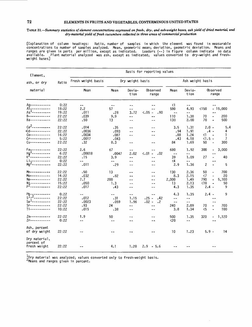
72 ELEMENTS IN FRUITS AND VEGETABLES, CONTERMINOUS UNITED STATES
TABLE 31.—Summary statistics of element concentrations expressed on fresh-, dry-, and ash-weight bases, ash yield of dried material, and dry-material yield of fresh cucumbers collected in three areas of commercial production
[Explanation of column headings: Ratio, number of samples in which the element was found in measurable concentrations to number of samples analyzed. Mean, geometric mean;, deviation, geometric deviation. Means and ranges are given in parts per million, except as indicated. Leaders (--) in figure column indicate no data available. Plant material analyzed was ash, except as indicated; values converted to dry-weight and fresh- weight bases]
Element,
ash, or dry
material
A ri_ _ _ _
Ai _ ___ _ _ __HI -------- Ac 1 _______
Da
fa 2
rr r_ _ _Cu —— —— - ———
Fe- — - ————H n-lg __________ifi
Li-——- —
M«
Mo ———————N-,Nj— — -----
Pb_- _______Sl' 2~— _—Se 1— — — -$r ______ _
Zn — — — —Zr — — — _—
Ash, percent of dry weight
Dry material, percent of fresh weight
^Dry material
Basis for reporting values
Ratio Fresn wei Qht basis
0:22 18:22 19:22 22:22 22:22
22:22 22:22 16:22 5:22
22:22
22:22 6:22
22:22 0:22
22:22
22:22 14:22 22:22 15:22 22:22
0:22 22:22 22:22 22:22 10:22
22:22 0:22
22:22
22:22
was analyzed;
Mean
2.2 .011 .039 .50
.014
.0036
.0034
.0017
.32
2.6 .00018 .15
.011
.50
.032 7.7 .050 .017
.012
.0023
.93
.015
1.9
values converted
Dry weight basis
Mean Devia- Observed tion range
57 .28 3.72 <.05 - .90
9.9 13
.35
.093
.087
.043 8.3
67 .0047 2.02 <.01 - .02
3.9
.29
13 .82
200 1.3 .43
.31 1.15 .25 - .42
.059 1.96 .02 - .2 24
.38
50
4.1 1.20 2.9 - 5.6
only to fresh-weight basis.
Ash weight basis
Mean
580
110 130
3.5 .94 .88 .43
84
680
39 <4 2.9
130 8.3
2,000 13 4.3
4.3
240 3.8
500 <20
10
Devia tion
4.93
1.38 2.00
1.31 1.91 1.24 4.18 1.69
1.92
1.09
1.36
2.36 2.15 1.49 2.13 1.35
1.35
2.09 1.34
1.35
1.23
<150
70 70
2
50
300
27
2
50 <7
790
2
2
70 <5
320
5
Observed range
- 15,000
200 500
.0 - 5.4
.4 - 4 1
.5 - 7 300
- 3,000
40
5
700 20
- 5,100 50
.4 - 9
.4 - 9
700 100
- 1,120
.9 - 14

TABLES 4-121 73
TABLE 32.—Summary statistics of element concentrations expressed on fresh-, dry-, and ash-weight bases, ash yield of dried material, and dry-material yield of fresh dry beans collected in four areas of commercial production
[Explanation of column headings: Ratio, number of samples in which the element was found in measurable concentrations to number of samples analyzed. Mean, geometric mean; deviation, geometric deviation. Means and ranges are given in parts per million, except as indicated. Leaders (--) in figure column indicate no data available. Plant material analyzed was ash, except as indicated; values converted to dry-weight and fresh- weight bases]
Element,
ash, or dry
material
Basis for reporting values
Ratio Fresn weight basis Dry weight basis Ash weight basis
Mean Mean Devia tion
Observed range
Mean Devia tion
Observed range
Ag——————- 2:40Al-—————— 15:40 2.7As 1 ———-—— 0:35B———————— 40:40 5.0Ba——————— 39:40 1.8
Ca 2 —————— 40:40 .090Cd——————— 35:40 .0086Co——————— 38:40 .16Cr——————— 6:40 .13Cu——————— 40:40 4.0
Fe-—————— 40:40 40Hg 1 ——————— 3:40 .0022K z ——————— 40:40 1.3Li-- ——— 2:40 .017Mg^—————— 40:40 .11
Mn——————— 40:40 6.3Mo——————— 40:40 2.8Na——————— 40:40 2.8Ni——- — -— 40:40 1.5pt——————— 40:40 .31
Pb--——— 0:40S 1 ^————--- 40:40 .16Se 1 — ———— 40:40 .026Sr——————— 40:40 5.6Ti——————— 7:40 .0060
Zn——————-- 40:40 26Zr———-——— 1:40
Ash, percent of dry weight
Dry material, percent of fresh weight
40:40
40:40
3.2 <.05 5.8 2.1
.11
.010
.19
.15 4.7
47.0026.3.020.13
7.4 3.3 3.3 1.8 .37
.19
.0306.6.0070
31
2.00 <.01 - .01
1.14 .162.29 .02
.28
.2
82
15055
2.7.26
4.83.9
120
1,200
39.52
3.3
1908485459.5
<20
170.18
790 <20
3.9
3.97 <150
3532
437555
4.971.45
1.53
1.042.931.33
1.392.421.771.781.12
2.542.87
1.14
1.09
70 <3
31,500
300150
1.5 -
70
700
35 <4 1.5
701525159
20 <5
580 <20
14100
- 300
- 3,000
4357
- 500- 300- 300- 150
12
700150
1,02030
3.4 - 4.9
85 1.07 5.5 - 93.7
Dry material was analyzed; values converted only to fresh-weight basis. Means and ranges given in percent.

74 ELEMENTS IN FRUITS AND VEGETABLES, CONTERMINOUS UNITED STATES
TABLE 33.—Summary statistics of element concentrations expressed on fresh-, dry-, and ash-weight bases, ash yield of dried material, and dry-material yield of fresh lettuce collected in four areas of commercial production
[Explanation of column headings: Ratio, number of samples in which the element was found in measurable concentrations to number of samples analyzed. Mean, geometric mean; deviation, geometric deviation. Means and ranges are given in parts per million, except as indicated. Leaders (--) in figure column indicate no data available. Plant material analyzed was ash, except as indicated; values converted to dry-weight and fresh-weight bases]
Element,
ash, or dry
material
A a _ _ __ _ ____ny-----------
A-l __ _________HI----------- Acl_ _____ ____
Ra
r ,2/-* j
Co —— - — - —r r_ _ _ _ _ ___Cu ——————
pe ————— ___iHa 1-———Vt.
Li- — — — -Mg<^ —————————
Mn ———————Mo ———————M-, ___
Ni ———————P*___________
Pb--- — — —sy_________Se 1 -- --------sr_ _ _ _ _ __T1— —————
Zn ———————Z r ——— -_ ——
Ash, percent of dry weight
Dry material , percent of fresh weight
*Dry material was Means and ranges
Ratio Fresn weight basis
1:40 33:40 16:29 40:40 40:40
40:40 40:40 10:40 13:40 40:40
40:40 24:40 40:40 13:40 40:40
40:40 2:40
40:40 15:40 40:40
2:40 40:40 38:39 40:40 16:40
40:40 10:40
40:40
40:40
analyzed given in
Mean
3.1
.55
.39
.025
.018
.0019
.34
5.6 .00035 .21 .012 .010
1.2 .0031
6.5 .042 .018
.029
.012
.0024 3.1
3.1 .024
; values converted percent.
Basis for reporting
Dry weight basis
Mean Devia- Observed tion range
73 <.02 1.3 9.4
.59
.42
.046
8.1
130 .0083 1.88 <.01 - .04
5.0 .28 .24
29 .074
150 1.0
.42
.70
.28 1.23 .16 - .4
.057 3.39 <.01 - .2 74
73 .56
4.2 1.34 2.9 - 8
only to fresgh-weight basis.
values
Ash weight basis
Mean
<1 520
93 67
4.2 3.0
.33 <1.5 58
960
36 2.0 1.7
210 .53
1 1 ,000 7.2 3.0
5.0
530
520 4.0
14
Devia tion
8.04
1.41 2.90
1.33 2.47 3.06
1.57
2.74
1.22 2.72 1.35
1.45 4.22 3.64 1.61 1.63
2.15
2.20
1.85 9.55
1.56
<1 <150
50 7
2
<1 <1 20
300
18 <4
70 <7
1,600 <10
<20
100 <5
150 <20
1
Observed range
2 - 30,000
300 500
.0 - 6.6
.8 - 14 4
.5 - 70 100
- 1,500
42 9
.7 - 3
500 15
- 64,000 20
.6 - 4.8
30
- 2,000 - 5,000
- 3,360 300
.8 - 29
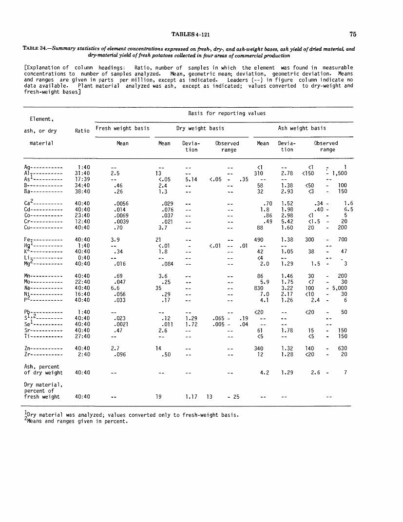
TABLES 4-121 75
TABLE 34.—Summary statistics of element concentrations expressed on fresh-, dry-, and ash-weight bases, ash yield of dried material, and dry-material yield of fresh potatoes collected in four areas of commercial production
[Explanation of column headings: Ratio, number of samples in which the element was found in measurable concentrations to number of samples analyzed. Mean, geometric mean; deviation, geometric deviation. Means and ranges are given in parts per million, except as indicated. Leaders (--) in figure column indicate no data available. Plant material analyzed was ash, except as indicated; values converted to dry-weight and fresh-weight bases]
Element,
ash, or dry
material
AnA1-Ml- ----------Ac 1 --- ___ ____MO —————————
D n
fa 2P _iCo-----------(Y-----------Cu ————————
Fe- — — — — -Hnli/Z_
Li-— — ... -Mg^ ——— - —— --
Mn ———————Mo ————— - —Ma
Ni— — — --p2_. _________
Ph — - ————S i>2_________se i~~ — —$r-----------Ti —— - — - —
Zn ———————Zr-— — - —
Ash, percent of dry weight
Dry material, percent of fresh weight
Basis for reporting values
Ratio frres '1 weight basis Dry weight basis
1:40 31:40 17:39 34:40 38:40
40:40 40:40 23:40 12:40 40:40
40:40 1:40
40:40 0:40
40:40
40:40 22:40 40:40 16:40 40:40
1:40 40:40 40:40 40:40 27:40
40:40 2:40
40:40
40:40
Mean
2.5
.46
.26
.0056
.014
.0069
.0039
.70
3.9
.34
.016
.69
.047 6.6
.056
.033
.023
.0021
.47
2.7 .096
Mean
13 <.05 2.4 1.3
.029
.076
.037
.021 3.7
21 <.01 1.8
.084
3.6 .25
35 .29 .17
.12
.011 2.6
14 .50
19
Devia- Observed Mean tion range
<1310
5.14 <.05 - .35 58 32
.70 1.8
.86
.49 88
490 <.01 -- .01
42 <4 2.0
86 5.9
830 7.0 4.1
<20 1.29 .065 - .19 1.72 .005 - .04
61 <5
340 12
4.2
1.17 13 - 25
Ash weight basis
Devia tion
2.78
1.38 2.93
1.52 1.98 2.98 5.42 1.60
1.38
1.05
1.29
1.46 1.75 3.22 2.17 1.26
1.78
1.32 1.28
1.29
<1<150
<50 <3
<1 <120
300
38
1
30 <7
100 <10
2
<20
15 <5
140 <20
2
Observed range
1 - 1,500
100 - 150
.34 - 1.6
.40 - 6.5 5
.5 - 20 - 200
- 700
47
.5 - "3
- 200 30
- 5,000 30
.4 - 6
50
150 - 150
- 630 20
.6 - 7
Dry material was analyzed; values converted only to fresh-weight basis. Means and ranges given in percent.

76 ELEMENTS IN FRUITS AND VEGETABLES, CONTERMINOUS UNITED STATES
TABLE 35.—Summery statistics of element concentrations expressed on fresh-, dry-, and ash-weight bases, ash yield of dried material, and dry-material yield of fresh snap beans collected in five areas of commercial production
[Explanation of column headings: Ratio, number of samples in which the element was found in measurable concentrations to number of samples analyzed. Mean, geometric mean; deviation, geometric deviation.Means and ranges are given in parts per million, except as indicated, indicate no data available. Plant material analyzed was ash, except as dry-weight and fresh-weight bases]
Leaders (--) in figure column indicated; values converted to
Element,
ash, or dry
material
An---Al-----------Ml- —————— -A<-1_ __ ____ ___
R a
fa 2PICo ————— —f>---------Cu ————— - — —
Fe —— - ------HoiK^-----------L1-— — —— -Mg^ —— - ——— -
Mn ———————Mo ———————l\la______
Ni ———————p*..-- .......
Rh —— _ ———— .
Si' 2— — —sei— — — --Jt
$r ———————Ti— —————
Zn ———————Zr ———————
Ash, percent of dry weight
Dry material , percent of fresh weight
Ratio
1:42 42:42 4:37
42:42 42:42
42:42 42:42 23:42 31:42 42:42
42:42 4:42
42:42 9:42
42:42
42:42 41:42 42:42 40:42 42:42
0:42 42:42 42:42 42:42 42:42
42:41 6.42
42:42
42:42
Fresh weight basis
Mean
7.3 .00074
1.4 .77
.060
.0026
.0059
.018
.56
9.2 .00033 .27 .0040 .031
2.3 .23
2.8 .18 .034
.019
.0031 2.4 .35
4.2 .28
Basis for reporting
Dry weight basis
Mean Devia- Observed tion range
66 .0067 3.85 <.05 - .1
13 7.0
.55
.024
.054
.16 5.1
84 .0030 1.92 <.01 - .01
2.4 .036 .28
21 2.1
25 1.7 .31
.17 1.27 .1 - .26
.028 1.51 .02 - .08 22 3.2
38 2.6
11 1.70 5.9 - 31
values
Mean
<1950
180 100
7.
2. 73
1,200
35 4.*
300 30
360 24 4.
<20
310 45
550 37
7.
Ash weight
Devia tion
2.43
1.43 2.73
8 1.30 34 1.89 77 2.55 3 2.66
1.53
1.52
1.06 52 1.01 0 1.45
1.72 2.74 2.05 1.72
4 1.16
1.75 2.60
1.22 1.95
0 1.20
basis
<1200
100 7
4
<1 <130
700
31 <5
1
150 <7
100 <10
3
707
400 <20
5
Observed range
1 - 7,000
- 300 - 700
.2 - 11
.2 - 1 7
.5 - 15 - 300
- 3,000
40 27 10
- 1,000 - 200 - 650
70 .6 - 6
- 700 - 500
- 800 - 100
.4 - 10
Dry material was analyzed; values converted only to fresh-weight basis. Means and ranges given in percent.
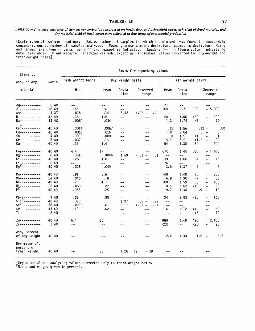
TABLES 4-121 77
TABLE 36.—Summery statistics of element concentrations expressed on fresh-, dry-, and ash-weight bases, ash yield of dried material, and dry-material yield of fresh sweet corn collected in four areas of commercial production
[Explanation of column headings: Ratio, number of samples in which the element was found in measurable concentrations to number of samples analyzed. Mean, geometric mean; deviation, geometric deviation. Means and ranges are given in parts per million, except as indicated. Leaders (--) in figure column indicate no data available. Plant material analyzed was ash, except as indicated; values converted to dry-weight and fresh-weight bases]
Element,
ash, or dry
material
An—Ai _ _____ _ __Mlr ---------As 1 —-— —
D -.
fa 2PICo ————(V-----------Cu ----------
FP -----------Hnl
1 !___________L|M,,<L
Mn ————— ---Mo ———————MaMi— - — — — — mp2___________
Ph ———————T 9sy_— - —
S P 1- __ __oc$r--- — _ ----Ti ————— —
Zn ——— -----Zr —————— —
Ash, percent of dry weight
Dry material , percent of fresh weight
Ratio Fresn weight basis Dry
0:40 18:40 3:37
32:40 13:40
40:40 40:40 4:40 5:40
40:40
40:40 8:40
40:40 0:40
40:40
40:40 24:40 40:40 20:40 40:40
3:40 40:40 38:40 33:40
2:40
40:40 1:40
40:40
40:40
Mean
.65
.025
.38
.0084
.0014
.0065
.0020
.037
.35
4.4 .0012 .25
.025
.91
.045 1.2
.055
.063
.22
.028
.0028
.10
6.4
Mean
2.6 .10
1.5 .034
.0057
.026
.0081
.15 1.4
17 .0046
1.0
.099
3.6 .18
4.7 .22 .25
.88
.11
.011
.42
25
25
Basis for reporting values
weight basis Ash weight basis
Devia- Observed Mean tion range
<]100
3.32 <.05 - .4 58 1.3
.22 1.0
.31 5.7
54
670 1.69 <.01 - .01
39 <4 3.8
140 6.9
180 8.5 9.7
34 1.37 .05 - .22 2.17 <.01 - .04
16
980 <20
2.6
1.28 12 - 39
Devia tion
3.71
1.56 5.79
1.56 2.84 1.91 3.51 1.38
1.48
1.06
1.37
1.40 1.98 1.59 1.62 1.34
2.53
1.72
1.49
1.34
Observed range
100
<50 <3
.12
.2 <1 <1.5 30
300
34
2
70 <7 50
<10 .9
<20
<10 <5
420 <20
1.2
- 5,000
100 30
.80 6.5 1
30 - 100
- 1,500
43
7
- 300 30
- 400 20 12
- 100
30 70
- 2,100 20
5.5
,Dry material was analyzed; values converted only to fresh-weight basis. •Means and ranges given in percent.

78 ELEMENTS IN FRUITS AND VEGETABLES, CONTERMINOUS UNITED STATES
TABLE 37.—Summary statistics of element concentrations expressed on fresh-, dry-, and ash-weight bases, ash yield of dried material, and dry-material yield of fresh tomatoes collected in five areas of commercial production
[Explanation of column headings: Ratio, number of samples in which the element was found in measurable concentrations to number of samples analyzed. Mean, geometric mean; deviation, geometric deviation. Means and ranges are given in parts per million, except as indicated. Leaders (--) in figure column indicate no data available. Plant material analyzed was ash, except as indicated; values converted to dry-weight and fresh- weight bases]
Element,
ash, or dry
material
AnAl___ __ _____ HI- ———————— -«<-!__ _ ______
Ra____ _ ___
Ca 2r ACo-— — —Cr-----------Cu—— —— - ——
Fe ————— --HnlHg ————————v?-H_ _ _ ___ _ _LI -M~.£
M M
Mo ———————Na— — — --Ni— — — -p2 — ________
PS _________Si»2_______._se i— — — -oc c«*
T1— — — —
Zn ———————Zr— —— -—
Ash, percent of dry weight
Dry material , percent of fresh weight
Ratio
0:50 30:50 8:50
49:50 40:50
50:50 48:50 16:50 13:50 50:50
50:50 5:50
50:50 0:50
50:50
50:50 30:50 50:50 10:50 50:50
0:50 50:50 49:49 50:50 15:50
50:50 0:50
50:50
50:50
Fresh weight basis
Mean
1.1 .00046 .52 .11
.0074
.0059
.0032
.0039
.46
3.0 .00016 .21
.011
.62
.042 21
.022
.015
.011
.0018
.52
1.4
Basis for reporting
Dry weight basis
Mean Devia- Observed tion range
20 .0089 4.80 <.05 - .25
10 2.0
.14
.11
.062
.074 8.8
58 .0031 1.91 <.01 - .01
4.1
.20
12 .82
410 .43 .29
.21 1.21 .14 - .33
.036 2.86 .01 - .35 10
26
5.2 1.43 1.8 - 8.9
values
Ash
Mean
<1170
84 17
1.2 1
.52
.62 73
480
34 <4 1.7
100 6.8
3,400 3.6 2.4
<20
83
220 <20
12
weight
Devia tion
4.92
1.39 4.45
1.69 2.87 1.95 2.99 1.68
1.90
1.18
1.34
1.68 2.08 2.26 2.79 1.41
2.33
1.62
1.25
basis
Observed range
<150 - 1
<50 - <3 -
.8 - <.2 -
<1 - <1.5 - 30 -
200 -
23 -
.7 -
50 - <7 -
900 - 26 <10 -
1.2 -
20 - <5 -
80 -
6.9 -
,500
150 150
3.2 10
4 7
200
500
45
3
500 30
,000 30 4.8
300 150
620
17
•;Dry material was analyzed; values converted only to fresh-weight basis. Means and ranges given in percent.

TABLES 4-121 79
TABLE 38.—Element concentrations expressed on fresh, dry, and ash weight bases, ash yield of dried material, and dry-material yield offresh asparagus from San Joaquin County, California
[Explanation of column headings: Ratio, number of samples in which the element was found in measurable concentrations to number of samples analyzed. Mean, geometric mean; deviation, geometric deviation. Means and ranges are given in parts per million, except as indicated. Leaders (--} in figure column indicate no data available. Plant material analyzed was ash, except as indicated; values converted to dry-weight and fresh- weight bases]
Element,
ash, or dry
material
AnAl-_- _ ____ _Ml--- flc-1--- __ _ __
D •»
r ,2r~ j
Co- — — —fY---------Cu ———————
Fe-~- - — —Hnil/Z_Li —————— -Mg^ ——————
Mn— —————Mo ———————Ma
Ni— - — — -p2________.._
Pb-__ ___ -__S?.2_______Se 1 — ----- ~$r ___ _ -__Ti ———————
7n------ _ -__Zr_- —
Ash, percent of dry weight
Dry material , percent of fresh weight
k)ry material
Ratio Fresh weight basis
0:10 7:10 1:9
10:10 10:10
10:10 10:10 3:10 1:10
10:10
10:10 2!: 10
10:10 4:10
10:10
10:10 7:10
10:10 5:10
10:10
0:10 10:10 10:10 10:10 8:10
10:10 0:10
10:10
10:10
was analyzed,
Mean
2.3
1.0 .23
.021
.0025
.0045
.95
4.7 .00036 .33 .022 .014
1.1 .054
23 .068 .043
.051
.045 4.0
7.3
values converted
Basis for reporting
Dry weight basis
Mean Devia- Observed tion range
29 <.05 — <.05 - .05
13 2.9
.27
.032
.057
12
60 .0046 1.69 <.01 - .01
4.2 .28 .18
14 .68
290 .86 .55
.65 1.07 .62 - .72
.57 1.12 .45 - .65 50
92
7.9 1.10 6.3 - 8.6
only to fresh-weight basis.
values
Mean
<1290
130 29
2.7 .32 .57
<1.5 120
600
42 2.8 1.8
140 6.8
2,900 8.6 5.5
<20
500
920 <20
10
Ash weight
Devia tion
basis
Observed range
4.31 <150 - 3,
1.31 70 - 1.40 20 -
1.10 2.4 - 1.51 .2 - 1.56 <1
<1.5 - 1.30 100 -
1.68 300 - 2,
1.04 39 - 1.48 <4 - 1.16 1.5 -
1.31 70 - 1.49 <7 - 1.26 2,200 - 4, 1.60 <10 - 1.12 4.8 -
1.36 300 <5 - 1,
1.09 810 - 1
1.09 9.0 -
000
150 50
3.2 .6
1 3
200
000
46 5 2
200 15
300 15 6.0
700 500
,030
12
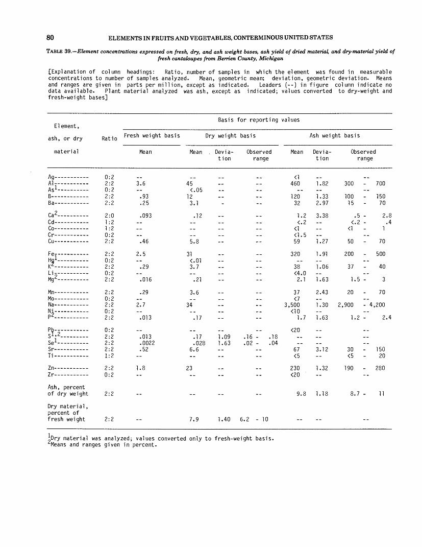
80 ELEMENTS IN FRUITS AND VEGETABLES, CONTERMINOUS UNITED STATES
TABLE 39.—Element concentrations expressed on fresh, dry, and ash weight bases, ash yield of dried material, and dry-material yield offresh cantaloupes from Berrien County, Michigan
[Explanation of column headings: Ratio, number of samples in which the element was found in measurable concentrations to number of samples analyzed. Mean, geometric mean; deviation, geometric deviation. Means and ranges are given in parts per million, except as indicated. Leaders (--) in figure column indicate no data available. Plant material analyzed was ash, except as indicated; values converted to dry-weight and fresh-weight bases]
Element,
ash, or dry
material
An
A 1
n _,
fa 2
Pr r _ _ ________Cu -----------
Fe ----------Ha*1/2Li- —— —— —— -
Mn — ——— —Mo —— ————
Ni ——— — —P2
cl,2s lQ r_ __ ________
Zn — — ———Zr — ———— _
Ash, percent of dry weight
Dry material , percent of fresh weight
Basis for reporting values
Ratio Fresl1 wei 9ht basis Dry weight basis
0:2 2:2 0:2 2:2 2:2
2:0 1:2 1:2 0:2 2:2
2:2 0:2 2:2 0:2 2:2
2:2 0:2 2:2 0:2 2:2
0:2 2:2 2:2 2:2 1:2
2:2 0:2
2:2
2:2
Mean
3.6
.93
.25
.093
.46
2.5
.29
.016
.29
2.7
.013
.013
.0022
.52
1.8
Mean .
45 <.05
12 3.1
.12
5.8
31
3.' 7
.21
3.6
34
.17
.17
.028 6.6
23
7.9
Devia- Observed Mean tion range
460
120 32
1.2
59
320
38 <4.0 2.1
37 <7
3,500
1.7
<20 1.09 .16 - .18 1.63 .02 - .04
67 <5
230 <20
9.8
1.40 6.2 - 10
Ash weight basis
Devia tion
1.82
1.33 2.97
3.38
1.27
1.91
1.06
1.63
2.43
1.30
1.63
3.12
1.32
1.18
Observed range
300 - 700
100 - 150 15 - 70
.5 - 2.8 <.2 - .4
<1 - 1
50 - 70
200 - 500
37 - 40
1.5 - 3
20 - 70
2,900 - 4,200
1.2 - 2.4
30 - 150 <5 - 20
190 - 280
8.7 - 11
material was analyzed; values converted only to fresh-weight basis. Means and ranges given in percent.

TABLES 4-121 81
TABLE 40.— Element concentrations expressed on fresh, dry, and ash weight bases, ash yield of dried material, and dry-material yield offresh Chinese cabbage from Palm Beach County, Florida
[Explanation of column headings: Ratio, number of samples in which the element was found in measurable concentrations to number of samples analyzed. Mean, geometric mean; deviation, geometric deviation. Means and ranges are given in parts per million, except as indicated. Leaders (—) in figure column indicate no data available. Plant material analyzed was ash, except as indicated; values converted to dry-weight and fresh- weight bases]
Element,
ash, or dry
material
AnA1---_- -- -Ml-- ——— ——— -flc-l. _____ _____ _
R a
Ca 2— — — -p_iCo ———————o _ _ _ ____W ———————————
Cu ————— —
Fe ———————i Ho 1 - —— —— ——
i/2Li _______Mg^ —————————
Mn ———————Mo ——— - —— -Na— ----- —Nj™. — .... p2___________
Ph ———————S l>2_________se i— — -—$r ___ ___ _Ti~— ------
Zn— — — -Zr —
Ash, percent of dry weight
Dry material , percent of fresh weight
Basis for reporting values
Ratio
0:2 1:2 2:2 2:2 2:2
2:2 0:2 0:2 0:2 2:2
2:2 1:2 2:2 0:2 2:2
2:2 1:2 2:2 0:2 2:2
0:2 2:2 2:2 2:2 0:2
2:20:2
2:2
2:2
Fresh weight basis
Mean
.013
.82
.82
.069
.15
2.1
.38
.015
.49
82
.028
.031
.00035 14
3.5
Dry weight basis
Mean Devia- Observed tion range
.26 1.49 .2 - .35 17 17
1.4
3.0
4.2 <.01 - <.01 - .01 7.8
.30
10
170
.58
.64 1.01 .64 - .65
.0071 1.63 .005 - .01 280
72
4.9 1.11 4.6 - 5.3
Mean
<1<150
80 80
7.0 <.2
<1 <1.5 15
210
39 <4 1.5
50 <7
8,400 <10
2.9
<20
1,400 <5
360 <20
20
Ash weight basis
Devia- Observed tion range
<150 - 200
1.29 70 - 100 1.29 70 - 100
1.20 6.2 - 8.0
1.00
1.63 150 - 300
1.00
1.00
1.00 <7 - 7
1.13 7,700 - 9,200
1.33 2.4 - 3.6
1.63 1,000 - 2,000
1.06 350 - 380
1.07 19 - 21
Dry material was analyzed; values converted only to fresh-weight basis. Means and ranges given in percent.
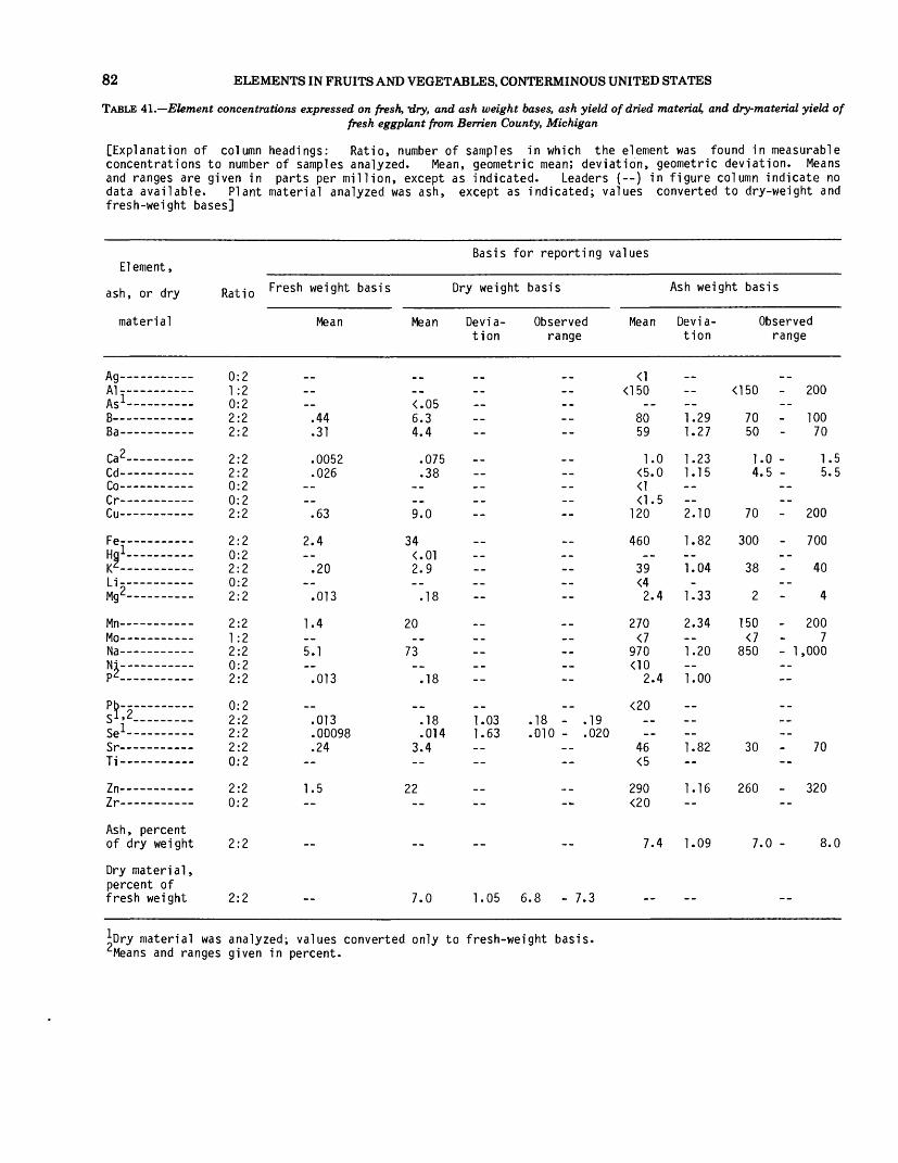
82 ELEMENTS IN FRUITS AND VEGETABLES, CONTERMINOUS UNITED STATES
TABLE 41.—Element concentrations expressed on fresh, tfry, and ash weight bases, ash yield of dried material, and dry-material yield offresh eggplant from Berrien County, Michigan
[Explanation of column headings: Ratio, number of samples in which the element was found in measurable concentrations to number of samples analyzed. Mean, geometric mean; deviation, geometric deviation. Means and ranges are given in parts per million, except as indicated. Leaders (--) in figure column indicate no data available. Plant material analyzed was ash, except as indicated; values converted to dry-weight and fresh-weight bases]
Element,
ash, or dry
material
An--------- _ag--------- — Al-----------Hl- ————————Ac 1 - ___ _ ___rvo
D i
fa 2/"* -4Cd- — ———— —Co- ——————r>_ _ _____Cu ———————
Fe--— — —Ha 1— ------yc.
Li————— —Mg^ ——————
Mn ———————Mo ———————NaNi— — -----pt
Pb-- ——— -S*jZ~~~-Se 1 - ———— _ocSr----- _ ----Ti_ _ _ _ __
Zn ———————7r------___ _
Ash, percent of dry weight
Dry material , percent of fresh weight
Basis for reporting values
Ratio Fresh weight basis Dry weight basis
0:2 1:2 0:2 2:2 2:2
2:2 2:2 0:2 0:2 2:2
2:2 0:2 2:2 0:2 2:2
2:2 1:2 2:2 0:2 2:2
0:2 2:2 2:2 2:2 0:2
2:2 0:2
2:2
2:2
Mean
.44
.31
.0052
.026
.63
2.4
.20
.013
1.4
5.1
.013
.013
.00098
.24
1.5
Mean
<.05 6.3 4.4
.075
.38
9.0
34 <.01 2.9
.18
20
73
.18
.18
.014 3.4
22
7.0
Devia- Observed Mean tion range
<1<150
80 59
1.0 <5.0 <1 <1.5
120
460
39 <4 2.4
270 <7
970 <10
2.4
<20 1.03 .18 - .19 1.63 .010 - .020
46 <5
290 <20
7.4
1.05 6.8 - 7.3
Ash weight basis
Devia tion
1.29 1.27
1.23 1.15
2.10
1.82
1.04
1.33
2.34
1.20
1.00
1.82
1.16
1.09
<150
70 50
1 4
70
300
38
2
150 <7
850
30
260
7
Observed range
- 200
100 70
.0 - 1.5
.5 - 5.5
- 200
- 700
40
4
- 200 7
- 1,000
70
- 320
.0 - 8.0
Dry material was analyzed; values converted only to fresh-weight basis Means and ranges given in percent.

TABLES 4-121 83
TABLE 42.—Element concentrations expressed on fresh, dry, and ash weight bases, ash yield of dried material, and dry-material yield offresh endive from Palm Beach County, Florida
[Explanation of column headings: Ratio, number of samples in which the element was found in measurable concentrations to number of samples analyzed. Mean, geometric mean; deviation, geometric deviation. Means and ranges are given in parts per million, except as indicated. Leaders (--) in figure column indicate no data available. Plant material analyzed was ash, except as indicated; values converted to dry-weight and fresh-weight bases]
Element,
ash, or dry
material
A a____ _ _____M y
Ai__- _ ___ _ _i Ac 1 ----------Mo ________
D =
fa 2p_iCo ——— - — -o_ _ ____ _ _C U ——— . _____
Fe — _.___—_Ga — — — — _HnlHg __________i/ZLi— ——— --
Mg 2 ————— _ ——Mn —_——_-_
N-,_ _____ _ __
P 2 ___________P h_ _______S 1 '^ ___ __Li---——
Ti ———— _____Zn ———————7«
Ash, percent of dry weight
Dry material , percent of fresh weight
Ratio
0:22:21:22:22:2
2:22:20:21:22:2
2:20:21:22:20:2
2:22:20:22:20:2
2:20:22:22:22:2
2:22:20:2
2:2
2:2
Fresh weight basis
Mean
1.21.2
(~\r o
.014
.99
12
BC;
.0124.2
250
.004012
.127.9
—
Basis for reporting values
Dry weight basis Ash
Mean Devia- Observed Mean tion range
<1101 -- -- 460
<.05 - .21 Q Q/l
18 -- -- 84
.90 -- -- 4.1
.22 — — 1.0<1.0
15 -- -- 70
190 -- -- 870<10
<.01 - .018 r OO
<4
1 Q Q/l
66 — -- 300<7
4,000 — — 18,500<10
• vJO i- • *T
<2077 1 no T 7 QQ
.06 1.91 .04 - .10180 -- -- 840
1.9 -- -- 9120 -- — 560
<20
22
6.4 1.05 6.2 - 6.6
weight basis
Devia- Observed tion range
1.82 300 - 700
1.29 70 - 1001.29 70 - 100
1.04 4.0 - 4.21.00
1.00
2.17 500 - 1,500
1.02 34 - 40
1.29 .70- 11.00
1.04 18,000 - 19,000
1.00
1.29 700 - 1,000
2.17 5 - 151.13 510 - 610
1.12 20 - 24
Dry material was analyzed; values converted only to fresh-weight basis. Means and ranges given in percent.
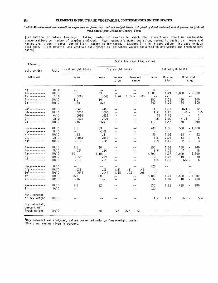
84 ELEMENTS IN FRUITS AND VEGETABLES, CONTERMINOUS UNITED STATES
TABLE 43.—Element concentrations expressed on fresh, dry, and ash weight bases, ash yield of dried material, and dry-material yield offresh onions from Hildalgo County, Texas
[Explanation of column headings: Ratio, number of samples in which the element was found in measurable concentrations to number of samples analyzed. Mean, geometric mean; deviation, geometric deviation. Means and ranges are given in parts per million, except as indicated. Leaders (--) in figure column indicate no data available. Plant material analyzed was ash, except as indicated; values converted to dry-weight and fresh-weight bases]
Element,
ash, or dry
material
An---- _ -Hy____
Al _ _________HI ————Ac-1 --- _ ___ _R _ ___ ___ ____
D a
r*2r* j
Co — — — --r r _ _ __ _ _Cu- ——— —— ——
Fe— — — -Ha— — .....\(£-
L1- — — ....Mg^ ————————
Mn ———————Mo ———————Ma _ _________
|\H_ _ ________I>M
p2 ————————
Ph ——— - ——sU---Se 1 -- -------Cv>____ __ __ __ _
Ti ——— _ ——
Zn ——— - ——Zr— — - — -
Ash, percent of dry weight
Dry material , percent of fresh weight
k)ry material
Ratio Fres '1 weight basis
0:10 10:10 7:10
10:10 10:10
10:10 10:10 4:10 2:10
10:10
10:10 0:10
10:10 2:10
10:10
10:10 5:10
10:10 10:10 10:10
0:10 10:10 10:10 10:10 10:10
10:10 0:10
10:10
10:10
was analyzed;
Mean
6.3 .0045
1.0 .88
.046
.0050
.0028
.0021
.46
3.3
.13
.0063
.012
1.6 .024
110 .059 .019
.033
.0042 8.8
.16
2.2
values converted
Basis for reporting
Dry weight basis
Mean Devia- Observed tion range
63 .045 1.74 <.05 - .05
10 8.8
.46
.050
.028
.021 4.6
33 <.01 1.3
.063
.12
16 .24
1,100 .59 .19
.33 1.21 .21 - .45
.042 1.38 .02 - .06 88
1.6
22
10 1.2 8.2 - 13
only to fresh-weight basis.
values
Mean
<1 1,500
250 200
111.2 .66 .5
110
780
30 1.6 2.8
390 5.6
2,700 13 4.6
<20
2,100 37
530 <20
4.2
Ash weight
Devia tion
1.21 1
1.35 1.39
1.13 1.23 1.46 3.00 1.42
1.35
1.05 2.23 1.19
1.56 1.75 1.27 1 1.26 1.16
1.23 1 1.87
1.28
1.17
basis
Observed range
,000 - 2,
150 - 150 -
8.4 - 1.0 -
<1 - <1.5 - 70 -
500 - 1,
28 - <4 -
2 -
150 - <7 -
,900 - 3, 10 - 3.6 -
,500 - 3, 10 -
420 -
3.1 -
000
300 500
12 1.5 1 3
200
000
32 6 3
700 15
800 20
6
000 100
980
5.4
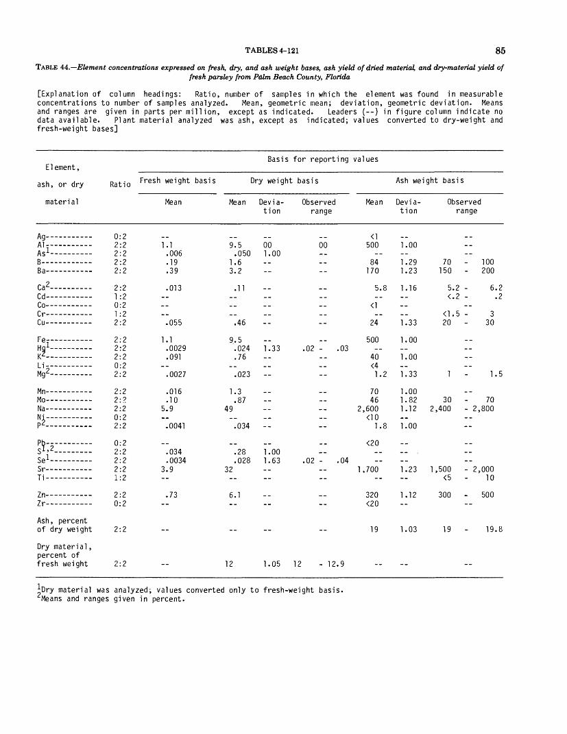
TABLES 4-121 85
TABLE 44.— Element concentrations expressed on fresh, dry, and ash weight bases, ash yield of dried material, and dry-material yield offresh parsley from Palm Beach County, Florida
[Explanation of column headings: Ratio, number of samples in which the element was found in measurable concentrations to number of samples analyzed. Mean, geometric mean; deviation, geometric deviation. Means and ranges are given in parts per million, except as indicated. Leaders (--) in figure column indicate no data available. Plant material analyzed was ash, except as indicated; values converted to dry-weight and fresh-weight bases]
Element,
ash, or dry
material
Al-----------rt l_ —————— _ A<; •*•----------
Ra
Ca 2— — — -r> A
Co ———————
Cu ———————
Fe--— — —H n iK ZLi- ——— - —
N'
p2 ————— . ——
Ql»2_ 1
SJ^
In ...........7 «
Ash, percent of dry weight
Dry material , percent of fresh weight
Ratio
0:2 2:2 2:2 2:2 2:2
2:2 1:2 0:2 1:2 2:2
2:2 2:2 2:2 0:2 2:2
2:2 2:2 2:2 0:2 2:2
0:2 2:2 2:2 2:21:2
2:2 0:2
2:2
2:2
Fresh weight basis
Mean
1.1 .006 .19 .39
.013
.055
1.1 .0029 .091
.0027
.016
.10 5.9
.0041
.034
.0034 3.9
.73
Basis for reporting
Dry weight basis
Mean Devia- Observed tion range
9.5 00 00 .050 1.00
1.6 3.2
.11
.46
9.5 .024 1.33 .02 - .03 .76
.023 —
1.3 .87
49
.034 --
.28 1.00
.028 1.63 .02 - .04 32
6.1
12 1.05 12 - 12.9
values
Mean
500
84 170
5.8
24
500
40 <4 1.2
70 46
2,600
1.8
<20
1,700
320 <20
19
Ash weight basis
Devia- Observed tion range
1.00
1.29 70 - 100 1.23 150 - 200
1.16 5.2 - 6.2 <.2 - .2
<1.5 - 3 1.33 20 - 30
1.00
1.00
1.33 1 - 1.5
1.00 1.82 30 - 70 1.12 2,400 - 2,800
1.00
1.23 1,500 - 2,000 <5 - 10
1.12 300 - 500
1.03 19 - 19.8
Dry material was analyzed; values converted only to fresh-weight basis. Means and ranges given in percent.

86 ELEMENTS IN FRUITS AND VEGETABLES, CONTERMINOUS UNITED STATES
TABLE 45.—Element concentrations expressed on fresh, dry, and ash weight bases, ash yield of dried material, and dry-material yield offresh peppers from Berrien County, Michigan
[Explanation of column headings: Ratio, number of samples in which the element was found in measurable concentrations to number of samples analyzed. Mean, geometric mean; deviation, geometric deviation. Means and ranges are given in parts per million, except as indicated. Leaders (--) in figure column indicate no data available. Plant material analyzed was ash, except as indicated; values converted to dry-weight and fresh- weight bases]
Element,
ash, or dry
material
n a _ _ ___Al---------__Ml --- ———Ac-1-----------R_ ___________D r>
fa 2r* A
Co- — - ———fr-----------Cu ———————
Fe _— — — _Hg 1 - —— - ———i/Z_Li-_ — ______Mg^ ————————
Mn ———————Mo —————— -Nfl----_Ni— — — --p2 —————— __
Ph.- —— _ ——Sl> 2— - _____s e i— — — -Sr ————— ---Ti ———————
7n---__- __-_Zr-- ————— -
Ash, percent of dry weight
Dry material , percent of fresh weight
^Dry material was Means and ranges
Ratio Fresn wei 9nt basis
0:2 1:2 1:2 2:2 2:2
2:2 2:2 0:2 0:2 2:2
2:2 0:2 2:2 0:2 2:2
2:2 0:2 2:2 2:2 2:2
0:2 2:2 2:2 2:2 0:2
2:2 0:2
2:2
2:2
analyzed given in
Mean
.65
.32
.0063
.016
1.1
5.4
.21
.016
1.4
8.4 .21 .019
.022
.015
.25
2.3
; values converted percent.
Basis for reporting
Dry weight basis
Mean Devia- Observed tion range
<.050 -- <.050 - .15 8.4 4.2
.081 --
.21
14
71 <.01 2.7
.20
18
109 2.7
.24
.28 1.03 .28 - .29
.02 1.00 3.3
30
7.7 1.32 6.3 - 9.3
only to fresh-weight basis.
values
Mean
<1 <150
100 50
.97 2.5
<1 <1.5
170
840
32 <4 2.5
210 <7
1,300 32 2.9
<20
39 <5
360 <20
8.4
Ash weight basis
Devia- Observed tion range
<150 - 300
1.00 1.00
1.19 .86 - 1.1 1.00
1.23 150 - 200
1.29 700 - 1,000
1.12 30 - 35
1.33 2.0 - 3.0
1.63 150 - 300
1.11 1,200 - 1,400 1.91 20 - 50 1.33 2.4 - 3.6
1.44 30 - 50
1.31 300 - 440
1.27 7.1 - 10
TABLES 4-121 87
TABLE 46.— Estimates of logarithmic variance for American grapes from three areas of commercial production in the conterminous United States
[Asterisk (*), significantly greater than zero at the 0.05 probability level]
Element, ash, Total Percent of total variance
. . n . Between Between fields Between sitesmaterial variance areas within areas within fields
Al ———————— 0.13430 8 <1 92B —— -__._—- .08212 <1 30 70Ba— — - —— - .05223 <1 *71 29Ca— — — — .03918 <1 11 89
Cd — ----- .10793 22 *36 42Cu—— - ———— - .02349 10 33 57 Fe 06621 *44 6 50K ———————— .01125 3 <1 98
Mg ——— - ——— .02664 <1 <1 100Mn- —— — —— .26212 63 31 6Na ———————— .25346 *66 5 29 p ———————— .01916 13 <1 87
S ———————— .02001 *32 *42 26Se ———————— .17675 *14 *68 18Sr ———————— .06267 *39 <1 61Zn— — —— — .04514 5 <1 95
Ash, percent of dry weight 1 2.0817 <1 <1 100
Dry material , percent of fresh weight 1 13.280 *73 *18 9
•^Variance calculated from nontransformed data.
TABLE 47.— Estimates of logarithmic variance for apples from five areas of commercial production in the conterminous United States
[Asterisk (*), significantly greater than zero at the 0.05 probability level]
Element, ash, Total Percent of total variance
. . , . Between Between fields Between sites material variance areas within areas within fields
Al ———————— 0.11593 7 9 84As ———————— .48775 16 *69 15B ———————— .03429 19 *43 38 Ba ———————— .07057 *29 17 54Ca ———————— .03937 *27 *33 40
Cd ———————— .04177 10 <1 90Cu ———————— .01669 <1 *34 66
K ———————— .00741 *29 12 59Mg ———————— .01219 10 17 74
Mn ———————— .09578 *71 8 21Na ———————— .01299 *44 *24 32p ———————— .00851 <1 2 98S ———————— .01937 *56 *16 28Sr— —————— .13136 *65 9 26
Ti ———————— .13626 *13 27 59Zn ———————— .02994 30 13 57
Ash, percent of dry weight 1 .34045 6 22 72
Dry material , percent of fresh weight 1 2.9988 *25 12 63
^Variance calculated from nontransformed data.
TABLE 48.— Estimates of logarithmic variance for European grapes from two areas of commercial production in the conterminous United States
[Asterisk (*), significantly greater than zero at the 0.05 probability level]
Element, ash, Total Percent of total variance
... . u Between Between fields Between sitesmaterial variance areas within areas within fields
Al ———————— 0.11966 <1 38 62B ———————— .03528 *34 <1 66Ba ———————— .17266 *57 <1 43Ca ———————— .19194 33 *36 31Cu ———————— .08430 *62 13 24
Fe ———————— .07541 *45 <1 55K ———————— .08214 *59 20 20 Mg ———————— .04905 *37 <1 63Mn ———————— .11491 *50 <1 50 Na ———————— .11169 *44 <1 56
P ———————— .10651 *70 7 23S- —— — —— .10453 *90 <1 9Sr ———————— .25664 *60 <1 40 Ti ———————— .23044 <1 24 76Zn — — — — — .06489 *37 13 50
Ash, percent of dry weight 1 1.0261 19 26 55
Dry material, percent of fresh weight 1 15.263 10 18 72
•'Variance calculated from nontransformed data.
TABLE 49.— Estimates of logarithmic variance for grapefruit from four areas of commercial production in the conterminous United States
[Asterisk (*), significantly greater than zero at the 0.05 probabilitylevel]
Element, ash, Total Percent of total variance
. . 1U Between Between fields Between sitesmaterial variance areas within areas within fields
Al ——— — —— 0.18569 *28 1 71B ———————— .02195 *46 <1 54Ba ———————— .11663 *41 <1 59Ca 04538 *49 4 47
Cu ———————— .02090 8 *48 44Fe ———————— .07494 *41 20 39K ———————— .00952 *27 16 57Mg ———————— .02833 14 <1 86
Mn ———————— .04002 *29 *28 43Na ——— - ——— .04525 *37 <1 63P ———————— .02385 *48 *20 32S ———————— .01256 *55 <1 45
Sr ———————— .14921 *69 <1 31Zn ——————— .01742 *38 20 42
Ash percent of dry weight 1 3.3243 *55 *18 27
Dry material , percent of fresh weight 1 4.1878 *64 2 34
Variance calculated from nontransformed data.
88 ELEMENTS IN FRUITS AND VEGETABLES, CONTERMINOUS UNITED STATES
TABLE 50.— Estimates of logarithmic variance for oranges from four areas of commercial production in the conterminous United States
[Asterisk (*), significantly greater than zero at the 0.05 probability level]
Element, ash, Total Percent of total variance
^ . . . 1U Between Between fields Between sites material variance areas witnin areas witnin fields
AT r\ onCQO *Qn Q CO
B ———————— .02640 *43 18 39Ba ———————— .16402 *87 3 10Ca ———————— .01416 *56 3 42
Cu ———————— .02426 3 7 90Fe ——————— .05171 11 *33 56K ———————— .00106 35 *26 39Mg— — ———— .01946 *18 12 70
Mn ———————— .03321 *1 5 <1 85Na ———————— .19940 *71 *14 15p ———————— .01466 *21 <1 79S— — — — — .00547 *29 <1 71
Sr ———————— .20647 *69 <1 31Zn ———————— .00847 <1 2 98
of dry weight 1 .47054 *51 <1 49
Dry material , percent of fresh weight 1 2.6117 *32 <1 69
Variance calculated from nontransformed data.
TABLE 51.— Estimates of logarithmic variance for peaches from four areas of commercial production in the conterminous United States
[Asterisk (*), significantly greater than zero at the 0.05 probability level]
. . , . Between Between fields Between sites material variance areas within areas within fields
Al — - ———— -- 0.25969 *30 <1 70B ———————— .03867 *28 24 48Ba ———————— .21549 *54 <1 46Ca ———————— .10072 *29 <1 71Cu — - ———— -- .08410 *32 <1 68
Fe--— ——— - .15377 *57 <1 43K ———————— .04595 <1 <1 TOOMg ———————— .03513 *17 <1 83 Mn— ———— - .10868 *56 <1 44
p ———————— .07165 *30 <1 70S ———————— .04409 *60 2 38Sr ————— — - .01048 *31 <1 69
Ash, percent or dry weight 1 9.0217 *26 17 57
Dry material , percent of fresh weight 1 14.447 *48 <1 52
Variance calculated from nontransformed data.
TABLE 52.— Estimates of logarithmic variance for pears from five areas of commercial production in the conterminous United States
[Asterisk (*), significantly greater than zero at the 0.05 probability level]
Element, ash, Total Percent of total variance
UIJf Iuy10 Between Between fields Between sites material variance areas within areas within fields
Al ——————— 0.18966 <1 <1 100B ———————— .03604 *23 11 66Ba — .—.._.. .07672 *27 13 61Ca- —— - — — .06188 7 31 62
Cd ———— - — - .11595 *44 6 50Cu ———————— .05219 52 93Fe-— — — - .06108 <1 31 68K ——— — ——— .02250 3 12 86
Mg ———————— .17080 28 89Mn ———————— .05080 <1 *53 47Na ———————— .16322 12 *48 40p ———————— .04623 6 26 68
S —————— - — .01651 *27 <1 73Se— —— — — .07863 *27 *41 32Sr ———————— .09763 8 20 72Zn ———————— .09304 3 *43 54
Ash, percent of dry weight 1 .44193 *66 3 30
Dry material , percent offresh weight 1 6.3830 *66 3 30
Variance calculated from nontransformed data.
TABLE 53.— Estimates of logarithmic variance for plums from four areas of commercial production in the conterminous United States
[Asterisk (*), significantly greater than zero at the 0.05 probability level]
Element, ash, Total Percent of total variance
material variance areas within areas within fields
Al ——— — - — 0.08467 66 88 B ———————— .04510 *41 5 54Ba ———————— .23738 *34 16 50Ca ———————— .02496 6 *50 44C U ———————— .10774 *56 <1 44
Fe ———————— .06557 *42 <1 58v nn?n <•! *d? <i7Mg ———————— .01684 7 31 62 Mn ———————— .08902 *62 <1 38Na ———————— .05059 8 29 63
p ———————— .06491 7 30 62S ———————— .01485 20 *36 44Se ——————— .06560 *36 16 48Sr ———————— .08641 8 *44 49Zn ———————— .11522 *27 *41 32
Ash, percent , of dry weight 1 6.2372 13 *59 28
Dry material , percent of fresh weight 1 12.674 *53 *33 14
Variance calculated from nontransformed data.
TABLES 4-121 89TABLE 54.— Estimates of logarithmic variance for cabbage from four
areas of commercial production in the conterminous United States
[Asterisk (*), significantly greater than zero at the 0.05 probability level]
Element, ash, Total Percent of total variance
. . . Between Between fields Between sitesmaterial variance areas within areas within fields
B ———————— 0.01742 13 10 77 Ba ———————— .20639 *B7 <1 12Ca ———————— .01028 *65 10 25Cd ———————— .12337 *51 17 33Co ———————— .04960 25 8 67Cu ———————— .01842 *17 <1 83
Fe ———————— .02521 27 <1 73K ————————— .00165 *57 5 38Li ———————— .04581 *61 <1 38Mg— — ----- .02495 13 <1 87Mn ———————— .01722 31 *35 34Mo ———————— .05389 *57 *27 15
Na ———————— .20808 *98 <1 2p ———————— .01747 32 25 42S ———————— .00709 *49 <1 51Se ———————— .15325 *66 <1 34Sr ———————— .07931 *75 7 18Zn ———————— .02067 *73 *15 12
Ash, percentof dry weight 1 4.8903 *73 7 20
Dry material , percent of fresh weight 1 2.1899 *62 10 28
Variance calculated from nontransformed data.
TABLE 55.— Estimates of logarithmic variance for carrots from two areas of commercial production in the conterminous United States
[Asterisk (*), significantly greater than zero at the 0.05 probability level]
Element, ash, Total Percent of total variance
material variance areas with1n areas within fields
B ———————— 0.01605 *23 <1 76Ba ———————— .30955 *86 *9 5Ca ——————— .00291 <1 15 85Cd ———————— .2160B *38 <1 62 Cu ———————— .02472 <1 <1 100
Fe— - —— —— .01305 <1 <1 100 K ——— - — —— .00059 2 <1 98Mg ———————— .02528 <1 12 88 Mn ———————— .00465 *84 3 13Ma ———————— .04469 *84 3 13
P noQOO *"5O XI CQ
S — .......... .01251 *60 <1 40
Sr- —— ----- .01634 <1 <1 100Zn ———————— .06779 *68 <1 32
of dry weight 1 1.6724 *28 <1 72
Variance calculated from nontransformed data.
TABLE 56.— Estimates of logarithmic variance for cucumbers from three areas of commercial production in the conterminous United States
[Asterisk (*), significantly greater than zero at the 0.05 probability level]
U ' y '°yiO Between Between fields Between sites
A] ———————— 0.38377 <1 18 B2As— — - ——— .30174 31 *64 5B ———————— .02395 20 <1 80Ba ——— - ——— .11491 *51 *30 19Ca ——————— .01863 <1 <1 100
Co ———————— .00646 *32 <1 6BCu ———————— .05763 22 30 48Fe ———————— .09482 *39 5 56 K—— —— ----- .00167 <1 *67 33
Mg ———————— .01925 12 21 67Mn ———————— .19782 *73 *15 12
N-j —— - ————— .06074 5 *78 17P ———————— .01843 17 4 79
S ———————— .00361 <1 36 64 Se ———————— .11629 *65 *18 17Sr— —— ——— .13853 *63 18 19Zn — — — — .02272 *65 4 31
Ash, percent of dry weight 1 4.9200 *35 15 50
percent of . fresh weight 1 .79488 4 <1 96
•'•Variance calculated from nontransformed data.
TABLE 57.— Estimates of logarithmic variance for dry beans from four areas of commercial production in the conterminous United States
[Asterisk (*), significantly greater than zero at the 0.05 probability Jevel]
. 1U Between Between fields Between sitesmaterial variance areas within areas within fields
B ———————— 0.02020 *17 <1 83Ba- — — — - .13673 *31 <1 69Ca ———————— .02982 *76 *13 11Cd— — — — .05180 *38 8 55Co- - _ ____.-. 17342 *54 11 34Cu ———————— .02697 3 *42 55
Fe 03815 *41 *23 36K ———————— .00027 11 <1 89Mg ———————— .02084 <1 <1 100Mn— ----- .02063 12 3 85Mo ———— ----- .17854 *76 3 21Na ———————— .07074 <1 <1 100
Ni ———————— .07732 *50 <1 50p ———————— .00324 *61 <1 39S ———————— .00339 *24 8 68Se ———————— .16469 *84 <1 16Sr ———————— .19947 *77 6 17Zn —— - ———— .00362 *39 *37 24
Ash, percent of dry weight 1 .12337 *35 10 55
Dry material , percent of , fresh weight 1 36.355 *36 *29 35
^Variance calculated from nontransformed data.

90 ELEMENTS IN FRUITS AND VEGETABLES, CONTERMINOUS UNITED STATES
TABLE 58.— Estimates of logarithmic variance for lettuce from four areas of commercial production in the conterminous United States
[Asterisk (*), significantly greater than zero at the 0.05 probability level]
Element, ash, Total Percent of total variance
. . , . Between Between fields Between sites matenal variance areas within areas within fields
Al ———————— 0.76786 *89 <1 10 B— — ----- . .02970 <1 <1 100Ba- — ----- — .26616 *84 1 15Ca ——————— .01873 *57 <1 43
Cd ———————— .19049 *83 <1 17Cu ———————— .04490 *60 13 28Fe ——————— .24585 *80 <1 20K-— --- —— .01187 *39 <1 61
Mg-— ----- .01784 9 18 73Mn ———————— .02864 *32 *26 42Na ——————— .40647 *97 <1 2p ———————— .05514 *78 1 21
S-— — — — .00934 *62 3 35Se——— ----- .34107 *92 <1 8Sr- —— - — — .15104 *86 <1 14Zn— — — — .07308 <1 *92 8
Ash, percent of dry weight 1 30.469 8 <1 92
Dry material , percent of fresh weight 1 2.3780 *65 *15 20
Variance calculated from nontransformed data.
TABLE 59.— Estimates of logarithmic variance for potatoes from four areas of commercial production in the conterminous United States
[Asterisk (*), significantly greater than zero at the 0.05 probability level]
Element, ash, Total Percent of total variance
,. . , . u Between Between fields Between sites material variance areas within areas within fields
Al ———————— 0.13469 *17 13 69B ———————— .01582 14 *42 44Ba ——————— .20911 *51 *37 12 Ca- —— - ——— .04021 *80 <1 19
Cd ———————— .09590 *30 *44 25 Cu ———————— .04633 *40 13 46 Fe ——————— .02020 9 <1 91K ———————— .00049 12 16 72
Mg— —————— .01324 *28 8 64Mn — - ————— .02960 *34 7 59 Na ——————— .32647 *91 *6 4p ————— . — . .01223 *38 <1 62
S ———————— .01419 *65 *18 17Se ———————— .06513 *55 <1 45Sr-- —————— - .07116 *47 *30 23 Ti ———— - ——— .27643 20 *39 41Zn ——————— .01549 17 *32 51
Ash, percent of dry weight 1 1.4361 *70 9 21
Dry material , percent of fresh weight 1 9.4412 *46 *37 17
^Variance calculated from nontransformed data.
TABLE 60.— Estimates of logarithmic variance for snap beans from five areas of commercial production in the conterminous United States
[Asterisk (*), significantly greater than zero at the 0.05 probability level]
Element, ash, Total Percent of total variance
. iu Between Between fields Between sites material variance areas w i t hin areas within fields
Al- — — ----- 0.16107 *35 *31 34B ———————— .02637 *36 13 51Ba ——————— .23149 *80 <1 20Ca 01516 *52 *35 13Cd ———————— .08245 *24 <1 76
Co ———————— .06705 11 *47 42Cr ———— ----- .11849 19 *55 26Cu —— - ———— .03798 *44 3 53Fe ——————— .03570 <1 9 91 K— —— - ——— .00080 *30 *44 26
Mg ———————— .02771 *26 *33 41 Mn ———————— .06063 *39 6 55Mo ———————— .22318 *82 *7 11Na ——————— .11192 *61 *26 13Mi ———————— .05533 *37 <1 62
p ———————— .00458 15 *53 32S — ----- - —— .01062 5 14 82Se- - 03735 *56 <1 44Sr-- —————— - .07973 *58 <1 42Ti ———————— .19610 *56 *17 26Zn ————— - — .00865 *63 <1 37
Ash, percent of dry weight 1 2.0250 *42 *44 14
Dry material , percent of fresh weight 1 70.435 *89 *6 5
Variance calculated from nontransformed data.
TABLE 61.— Estimates of logarithmic variance for sweet corn from four areas of commercial production in the conterminous United States
[Asterisk (*), significantly greater than zero at the 0.05 probability level]
Element, ash, Total Percent of total variance
iu Between Between fields Between sites material variance areas within areas within fields
B ———————— 0.03628 *36 <1 64Ca ——————— .04097 *41 *27 32 Cd ———————— .22368 28 *62 10 Cu ———————— .02094 8 <1 92Fe ———— - —— - .03115 *31 <1 69
K ———————— .00061 <1 12 88Mg ————— —— .01926 <1 23 77 Mn ——————— - .02192 93 89Na ——————— .04312 <1 12 88 D m OTQ ^i /l QQ
Se ————— - — .12375 *69 11 19 Sr — —— —— - .04675 *62 <1 37Zn ———————— .03610 *74 *16 10
Ash, percent of dry weight 1 .80232 *32 *43 24
Dry material , percent of , fresh weight 1 38.084 *53 *34 13
^Variance calculated from nontransformed data.

TABLES 4-121
TABLE 62.— Estimates of logarithmic variance for tomatoes from five areas of commercial produc tion in the conterminous United States
[Asterisk (*), significantly greater than zero at the 0.05 probability level]
91
Element, ash,or dry
material
D-,
Ca —— - ——— —r* JCd-- —— - —— -Cu ————————
FP _ __ _ __ _ _i/Mg —————————Mn __ __ __ _ _Na__
p —————————S-------------SP_ _ _ ___ __Sr _ __ _ _ __Zn— — - ———
Ash, percent of dry weight
Dry material, percent of fresh weight
TotalIo9l0
variance
0.02045OTCOO
.06251
.23011
.05758
.10148
.00562
.02104057521445^
noopn
.00774OOOQO
1546104834
6.9331
3.4890
Between areas
*97
*83\J\J
*32\J L.
*65\J *J
*66
*17*19*29*61*68
*/l O
*58+J\J
*59*J -/
*59*54
*56
*70
Percent of total
Between fields within areas
5*j<1<1
5*J13I <J
<124<1
2*16
1 O
3\J3\J
<1<1
<1
9
variance
Between sites within fields
6817CO
2920
OO
57713716
4039op
4145
44
21
Variance calculated from nontransformed data.
92 ELEMENTS IN FRUITS AND VEGETABLES, CONTERMINOUS UNITED STATES
TABLE 63.— Areas having significantly different concentrations of elements at the 0.05 probabilitylevel in fruits and vegetables
[Concentrations given in ash, except as indicated. Significance tested at the 95-percent confidence level]
Element, ash or dry material
Al , ppm — — — —
As, ppm —— -——
Ba, ppm —— — ——
Ca, percent — —
Cd, ppm ----- ——
Co, ppm ------
Cu, ppm — —— ——
Fe, ppm —— — ——
Kind of produce, and mean concen tration, all areas
Grapefruit, 380Orange, 430Peach, 430Lettuce, 520Potato, 310Snap bean, 950
Apple, 0.20Cucumber, 0.28
European grape, 370 Grapefruit, 170Orange, 260Peach, 380Pear, 440Plum, 370Snap bean, 180Sweet corn, 58Tomato, 84
Apple, 77European grape, 62Grapefruit, 77Orange, 86Peach, 18Pear, 150Plum, 32Cabbage, 52Carrot, 120Cucumber, 130Dry bean, 55Lettuce, 67Potato, 32Snap bean, 100Tomato, 17
Apple, 1.1Grapefruit, 5.9Orange, 7.8Peach, 0.29Cabbage, 6.6
Dry bean, 2.7Lettuce, 4.2Potato, 0.70Snap bean, 7.8Sweet corn, 0.22Tomato, 1.2
Pear, 0.27 Cabbage, 1.0
Carrot, 2.1Cucumber, 0.94Dry bean, 0.26Lettuce, 3.0Potato, 1.8Snap bean, 0.34Tomato, 1.0
Cucumber, 0.88 Dry bean, 4.8
European grape, 63Peach, 56Plum, 51Cabbage, 31Lettuce, 58Potato, 88Snap bean, 73Tomato, 73
American Grape, 430European grape, 490Grapefruit, 310Peach, 300Plum, 200Cucumber, 680Lettuce, 960Sweet corn, 670
Tomato, 480
Area; mean
High
Riverside County, Calif.; 810Riverside County, Calif.; 970Yakima County, Wash.; 1,200Cumberland County, N.J.; 11,000Cumberland County, N. J. ; 645Cumberland County, N.J.; 2,200
Berrien County, Mich.; 0.45Cumberland County, N.J.; 0.63
San Joaquin County, Calif.; 450 Hidalgo Co. , Tex. ; 240Riverside County, Calif.; 320Yakima County, Wash.; 560Yakima County, Wash.; 580Yakima County, Wash.; 610Twin Falls County, Idaho; 245Palm Beach County, Fla.; 85Berrien Co., Mich.; 110
Wayne County, N.Y. ; 130San Joaquin County, Calif.; 100Hidalgo County, Tex.; 160Hidalgo County, Tex.; 220Yakima County, Wash.; 55Berrien Co. , Mich.; 250Yakima County, Wash.; 60Berrien County, Mich.; 150Hidalgo County, Tex.; 270Berrien County, Mich.; 170San Joaquin County, Calif.; 110Cumberland County, N.J.; 157Cumberland County, N.J.; 81Wayne Co. , N.Y.; 210Berrien County, Mich.; 54
Wyane County, N.Y.; 1.6Hidalgo County, Tex.; 8.4Hidalgo County, Tex.; 8.6Yakima County, Wash.; 0.49Cumberland County, N.J. , and
Hidalgo County, Tex.; 7.7Mesa County, Colo. ; 4.5Palm Beach County, Fla.; 5.3Twin Falls County, Idaho; 1.3Wayne County, N.Y.; 9.6Palm Beach County, Fla.; 0.34Berrien County, Mich.; 1.8
Wayne County, N.Y. ; 0.68 Cumberland County, N.J. , and
Imperial County, Calif.; 1.7Imperial County, Calif.; 3.4Berrien County, Mich.; 1.5Mesa County, Colo.; 0.45Imperial County, Calif.; 8.7Yakima County, Wash.; 2.8Palm Beach County, Fla.; 0.56Berrien County, Mich.; 2.7
Berrien County, Mich.; 0.74 Mesa County, Colo.; 10
Yakima County, Wash.; 43Wayne County, N.Y. ; 83Wayne County, N.Y.; 92Berrien County, Mich.; 39Imperial County, Calif.; 84Cumberland County, N.J. ; 135Berrien County, Mich.; 170Palm Beach County, Fla.; 121
Yakima County, Wash.; 650San Joaquin County, Calif.; 680Riverside County, Calif.; 560Yakima County, Wash.; 750Wayne County, N.Y.; 280Berrien County, Mich.; 1,000Cumberland County, N.J.; 4,500Berrien County, Mich.; and
Salem County, N.J. ; 790Berrien County, Mich. ; 740
concentration
Low
Palm Beach County, Fla.; 150Palm Beach County, Fla.; 110Mesa County, Colo.; 220Palm Beach County, Fla.; 180Yakima County, Wash.; 195Berrien County, Mich.; 590
Mesa County, Colo.; 0.024Berrien Co., Mich.; 0.099
Yakima County, Wash.; 310 Palm Beach County, Fla.; 150Palm Beach County, Fla.; 177Wayne Co., N.Y.; 300San Joaquin County, Calif.; 340Berrien County, Mich.; 280Cumberland County, N.J.; 140Salem County, N.J.; 28Palm Beach County, Fla.; 65
Salem County, N.J.; 46Yakima County, Wash.; 36Palm Beach County, Fla.; 46Palm Beach County, Fla.; 40Mesa County, Colo.; 5.9San Joaquin County, Calif.; 100Mesa County, Colo.; 13Imperial County, Calif.; 22Imperial County, Calif.; 22Cumberland County, N.J.; 30Mesa County, Colo.; 29Imperial County, Calif.; 13Wayne County, N.Y.; 9.1Palm Beach County, Fla.; 22Palm Beach County, Fla.; <3
Gloucester County, N.J.; 0.82Yuma County, Ariz.; 3.6Yuma County, Ariz.; 2.0San Joaquin County, Calif.; 0.18Imperial County, Calif,; 5.5
Wayne County, N.Y.; 2.1Cumberland County, N.Y.; 3.1Wayne County, N.Y. ; 0.48Berrien County, Mich.; 5.5Salem County, N.J.; 0.16Palm Beach County, Fla.; 0.70
San Joaquin, Calif.; 0.13 Hidalgo County, Tex.; 0.59
Hidalgo County, Tex.; 1.3San Joaquin, Calif.; 0.60San Joaquin, Calif.; 0.20Palm Beach County, Fla.; 0.94Cumberland County, N.J.; 1.1Cumberland County, N.J. ; 0.23Palm Beach County, Fla. , and
San Joaquin County, Calif.; 0.38
Cumberland County, N.J.; <1 Wayne County, N.Y.; 1.9
San Joaquin County; Calif.; 29Mesa County, Colo.; 33Mesa County, Colo.; 29Cumberland County; N.J.; 24Cumberland County; N.J.; 36Wayne County, N.Y. ; 62Wayne County, N.Y.; 49San Joaquin County, Calif.; 37
Wayne County, N.Y.; 280Yakima County, Wash.; 360Palm Beach County, Fla.; 210Mesa County, Colo.; 140Mesa County, Colo.; 120San Joaquin County, Calif.; 480Hidalgo County, Texas; 534Twin Falls County, Idaho; 470
San Joaquin County, Calif.; 300
TABLES 4-121
TABLE 63.— Areas having significantly different concentrations of elements at the 0.05 probability level in fruits and vegetables—Continued
93
Element, ash, or dry material
K, percent -----
Li , ppm--- — ---
Mg, percent----
Mn, ppm----- — -
Mo, ppm--------
Na , ppm — ------
Ni , ppm-- — ----
P, percent-----
Pb, ppm--------
S, percent 1 - —
Kind of produce, and mean concen
tration, all areas
Apple, 35
European grape, 20Grapefruit, 36
Cabbage, 36Lettuce, 36Snap bean, 35
Grapefruit, 3.7 Orange, 5.3Pear, 1.1Cabbage, 4.9
Carrot, 2.3Lettuce, 2.0Snap bean, 0.52
Orange, 2.1Peach, 1.1Potato, 2.0Snap bean, 4.0Tomato, 1.7
Apple, 74European grape, 62Grapefruit, 34Orange, 43Peach, 42Plum, 53Carrot, 120Cucumber, 130Lettuce, 210Potato, 86Snap bean, 300Tomato, HO
Cabbage, 9.1
Dry bean, 84Snap bean, 30
American grape, 390 Apple, 600European grape, 770Grapefruit, 1,600Orange, 1,600Cabbage, 29,000Carrot, 4,800Cucumber, 2.000Lettuce, 11,000Potato, 830Snap bean, 360Tomato, 1,800
Dry bean, 45Snap bean, 24
European grape, 2.3Grapefruit, 3.0Orange, 2.7Peach, 1.5Cabbage, 3.2
Dry bean, 9.5Lettuce, 3.0Potato, 4.1Tomato, 2.4
Apple, <20 Pear, 9.8
American grape, 0.062Apple, 0.026Grapefruit, 0.066Orange, 0.067Peach, 0.043Pear, 0.029Cabbage, 0.72Carrot, 0.13Dry bean, 0.19Lettuce, 0.28Potato, 0.12Snap bean, 0.17Tomato, 0.21
Area; mean
High
Gloucester County, N.J. ; andMesa County, Colo.; 38
San Joaquin County, Calif.; 29Palm Beach County, Fla., and
Hidalgo County, Texas; 39Berrien County, Mich.; 40Hidalgo County, Texas, 39Berrien County, Mich.; 39
Yuma County, Ariz.; 12 Yuma County, Ariz.; 20Mesa County, Colo.; 7.3Imperial County, Calif.; 7.1
Imperial County, Calif.; 3.5Imperial County, Calif.; 6.0Twin Falls County, Idaho; 12
Palm Beach County, Fla.; 2.5Yakima County, Wash.; 1.5Wayne County, N.Y.; 2.4Wayne County, N.Y.; 5.4Berrien County, Mich.; 2.2
Wayne County, N.Y.; 130San Joaquin County, Calif.; 93Hidalgo County, Tex.; 47Palm Beach County, Fla.; 51Yakima County, Wash., 78Berrien County, Mich., 100Hidalgo County, Tex., 164Berrien County, Mich.; 283Cumberland County, N.J.; 253Cumberland County, N.J.; 114Wayne County, N.Y., 460Berrien County, Mich.; 215
Berrien County, Mich., and Cumberland County, N.J.; 15
Mesa County, Colo.; 240Twin Falls County, Idaho; 140
Yakima County, Wash.; 1,300 Gloucester County, N.J.; 1,200San Joaquin County, Calif.; 1,100Hidalgo County, Tex.; 2,100Riverside County, Calif.; 5,400Hidalgo County, Tex.; 46,000Imperial County, Calif.; 6,700San Joaquin County, Calif.; 2,700Imperial County, Calif.; 54,000Twin Falls County, Idaho; 3.900Twin Falls County, Idaho; 470San Joaquin County, Calif.; 11,000
San Joaquin County, Calif.; 78Berrien County, Mich.; 46
San Joaquin County, Calif.; 3.6Palm Beach County, Fla.; 3.5Palm Beach County, Fla.; 3.3Yakima County, Wash.; 2.4Berrien County, Mich., Cumberland
County, N.J. , and ImperialCounty Calif.; 3.6
San Joaquin County, Calif.; 11Imperial County, Calif.; 3.9Wayne County, N.Y. ; 4.4Berrien County, Mien., 3.2
Berrien County, Mich.; 54 Berrien County, Mich.; 16
Berrien County, Mich.; 0.071Gloucester County, N.J.; 0.034Riverside County, Calif.; 0.083Riverside County, Calif.; 0.075Wayne County, N.Y.; 0.068Wayne County, N.Y.; 0.035Imperial County, Calif.; 0.80Imperial County, Calif., 0.15San Joaquin County, Calif.; 0.21Cumberland County, N.J.; 0.34Cumberland County, N.J.; 0.16Palm Beach County, Fla.; 0.19Berrien County, Mich., and
Cumberland County, N.J.; 0.25
concentration
Low
Berrien County, Mich.; 29
Yakima County, Wash.; 14Yuma County, Ariz.; 29
Hidalgo County, Texas; 34Cumberland County, N.J.; 28Cumberland County, N.J.; 34
Palm Beach County, Fla.; <4 Palm Beach County, Fla.; <4All others; <4Berrien County, Mich., and
Cumberland County, N.J.; <4Hidalgo County, Tex.; <4Palm Beach County, Fla.; <4Palm Beach County, Fla.; <4
Yuma County, Ariz. ; 1.7Mesa County, Colo.; 0.97Cumberland County, N.J.; 1.2Palm Beach County, Fla.; 3.0Palm Beach County, Fla.; 1.3
Mesa County, Colo.; 29Yakima County, Wash.; 2.4Palm Beach County, Fla.; 24Yuma County, Ariz. ; 42Mesa County, Colo., 23Mesa County, Colo. ; 27Imperial Counmty, Calif.; 94Cumberland County, N.J.; 59Imperial County, Calif.; 154Twin Falls County, Idaho; 62Cumberland County, N.J.; 200Palm Beach County, Fla.; 73
Imperial County, Calif.; 6.1
Wayne County N.Y.; 31Wayne County, N.Y., 13
Berrien County, Mich.; 220Berrien County, Mich.; 350Yakima County, Wash.; 530Yuma County, Ariz.; 1,300Yuma County, Ariz.; 1 ,300Berrien County, Mich.; 4,500Hidalgo County, Tex.; 3.500Berrien County, Mich.; 1,500Cumberland County, N.J.; 2,200Wayne County, N.Y.; 310Wayne County, N.Y.; 170Cumberland County, N.J.; 1,300
Twin Falls County, Idaho; 26Palm Beach County, Fla.; 15
Yakima County, Wash., 1.4Yuma County, Ariz.; 2.0Riverside County, Calif.; 2.4Mesa County, Colo.; 1.0Hidalgo County, Tex.; 2.6
All others; 9Cumberland County, N.J.; 1.5Yakima County, Wash.; 0.46Palm Beach County, Fla.; 1.6
Yakima County, Wash.; <20 Yakima County, Wash., San Joaquin
County, Calif., and Mesa County,Colo.; <20
Yakima County, Wash.; 0.049Yakima County, Wash.; 0.018Hidalgo County, Tex.; 0.053Palm Beach County, Fla.; 0.060Yakima County, Wash.; 0.029Mesa County, Colo.; 0.023Berrien County, Mich.; 0.55Hidalgo County, Tex.; 0.11Twin Falls County, Idaho; 0.18Palm Beach County, Fla.; 0.22Twin Falls County, Idaho; 0.093Wayne County, N.Y.; 0.15San Joaquin County, Calif.; 0.16
94 ELEMENTS IN FRUITS AND VEGETABLES, CONTERMINOUS UNITED STATES
TABLE 63.—Areas having significantly different concentrations of elements at the 0,05 probability level in fruits and vegetables—Continued
Element, ash. or dry material
Se, ppm 1 - ------
Sr, ppm ------ -
Ti ppm --------
Zn, ppm -------
Zr2 , ppm ----- —
Ash, percentof dry weight-
Dry material ,percent offresh weight ---
Kind of produce, and mean concen
tration, all areas
American grape, 0.012 Pear, 0.0058Plum, 0.0057Cabbage, 0.15Carrot, 0.064Cucumber, 0.059Dry bean, 0.030Lettuce, 0.057Potato, 0.011Snap bean, 0.028Sweet corn, 0.011Tomato, 0.036
American grape, 160 Apple, 97
European grape, 240Grapefruit, 650Orange, 710Peach, 46Cabbage, 690
Cucumber, 240Dry bean, 170Lettuce, 530Potato, 61Snap bean, 310Sweet corn, 16Tomato, 83
oAmerican grape , 7.4 Apple, 10
Potato2 , 9.6Snap bean, 45
Apple, 67 European grape, 66Grapefruit, 130
Pear, 150Plum, 120Cabbage, 270Carrot, 290Cucumber, 500Dry bean, 790Snap bean, 550Sweet corn, 980Tomato, 220
Peach, 4.2Lettuce., 4.0Snap bean, 37
Grapefruit, 3.8Orange, 3.6Peach, 6.7Pear, 2.1Cabbage, 9.3Carrot, 7.1Cucumber, 10Dry bean, 3.9
Potato, 4.2Snap bean, 7.0Sweet corn, 2.6Tomato, 12
American grape, 16Apple, 14
Grapefruit, 10Orange, 13
Peach, 10Pear, 15Plum, 14
Cabbage, 7.8Carrot, 12Dry bean, 85Lettuce, 4.2Potato, 19Snap bean, 11Sweet corn, 25Tomato, 5.2
Area; mean
High
Yakima County, Wash.; 0.018 Mesa County, Colo.; 0.012Mesa County, Colo.; 0.011Imperial County, Calif.; 0.31Imperial County, Calif.; 0.13San Joaquin County, Calif.; 0.098Mesa County, Colo.; 0.11Cumberland County, N.J.; 0.078Yakima County, Wash.; 0.056Cumberland County, N.J.; 0.045Salem County, N.J.; 0.026San Joaquin County, Calif.; 0.16
Yakima County, Wash.; 250 Mesa County, Colo.; 207
San Joaquin County, Calif.; 470Riverside County, Calif.; 1,300Riverside County, Calif.; 1,400Yakima County, Wash.; 82Hidalgo County, Tex. , and
Imperial County, Calif.; 840San Joaquin County, Calif.; 420Mesa County, Colo.; 360Palm Beach County, Fla.; 1,000Yakima County, Wash.; 100Palm Beach County, Fla.; 470Palm Beach County, Fla.; 26San Joaquin County, Calif.; 280
Wayne County, N.Y.; 40 Berrien County, Mich., and
Yakima County, Wash.; 16Cumberland County, N.J.; 36Cumberland County, N.J.; 130
Gloucester County, N.J.; 86 San Joaquin County, Calif.; 87Hidalgo County, Tex., and
Riverside County, Calif.; 150Wayne County, N.Y.; 210Wayne County, N.Y. ; 208Imperial County, Calif.; 340Imperial County, Calif.; 417Berrien County, Mich.; 630Wayne County, N.Y.; 890Palm Beach County, Fla.; 730Palm Beach County, Fla.; 1,400Berrien County, Mich.; 370
Mesa County, Colo.; 9.6Cumberland County, N.J.; 75Cumberland County, N.J.; 16
Yuma County, Ariz.; 5.6Yuma County, Ariz.; 4.1Yakima County, Wash.; 8.9San Joaquin County, Calif.; 2.7Cumberland County, N.J.; 12Hidalgo County, Tex.; 7.6Cumberland County, N.J.; 12San Joaquin County, Calif.; 4.0
Cumberland County, N.J.; 5.8Cumberland County, N.J.; 8.0Palm Beach County, Fla.; 3.3Cumberland County, N.J. , and
Palm Beach County, Fla.; 14
Yakima County, Wash.; 20Berrien County, Mich., and
Yakima County, Wash.; 16Hidalgo County, Tex.; 13Hidalgo County, Tex., and
Riverside County, Calif.; 14Yakima County, Wash.; 14Mesa County, Colo.; 18Mesa County, Colo.; 18
Hidalgo County, Tex.; 8.9Imperial County, Calif.; 13Mesa County, Colo.; 90Cumberland County., N.J. ; 6.2Yakima County, Wash.; 21Twin Falls County, Idaho; 23Salem County, N.J.; 32Yakima County, Wash.; 6.4
concentration
Low
Wayne County N.Y.; 0.0076San Joaquin County, Calif.; 0.0035Yakima County, Wash.; 0.0036Cumberland County, N.J.; 0.057Hidalgo County, Tex.; 0.032Berrien County, Mich.; 0.034San Joaquin County, Calif.; 0.020Palm Beach County, Fla.; 0.008Cumberland County, N.J.; 0.009Wayne County, N.Y.; 0.020Palm Beach County, Fla.; 0.0048Palm Beach County, Fla.; 0.015
Berrien County, Mich.; 150 Berrien County, Mich., and
Gloucester County, N.J.; 46Yakima County, Wash.; 130Palm Beach County, Fla.; 260Palm Beach County, Fla.; 200Wayne County, N.Y.; 27Berrien County, Mich.; 200
Cumberland County, N.Y.; 84Wayne County, N.Y.; 46Cumberland County, N.J.; 157Wayne County, N.Y.; 40Berrien County, Mich.; 150Salem County, N.J.; 7.4Berrien County, Mich.; 52
Berrien County, Mich.; 2.8Wayne County, N.Y.; 3
Wayne County N.Y.; 2.5Twin Falls County, Idaho; 22
Yakima County, Wash.; 49 Yakima County, Wash.; 50Yuma County, Ariz.; 97
Mesa County, Colo.; 100Mesa County, Colo. ; 65Hidalgo County, Tex.; 210Hidalgo County, Tex.; 205Cumberland County, N.J.; 360Twin Falls County, Idaho; 700Wayne County, N.Y.; 490Twin Falls County, Idaho, 590San Joaquin County, Calif.; 130
All others; <20All others; <20Berrien County, Mich., Wayne
County N.Y., and Twin FallsCounty, Idaho; <2.0
Hidalgo County, Tex.; 2.6Hidalgo County, Tex.; 3.1San Joaquin County, Calif.; 6.0Mesa County, Colo.; 1.7Hidalgo County, Tex.; 7.7Imperial County, Calif.; 6.7Berrien County, Mich.; 8.7Twin Falls County, Idaho, and
Mesa County, Colo. ; 3.7Twin Falls County, Idaho; 3.3Berrien County, Mich.; 5.5Salem County, N.J.; 2.0Yakima County, Wash.; 6.4
Berrien County, Mich.; 14Wayne County, N.Y. , and
Gloucester County, N.J.; 14Yuma County, Ariz.; 8.6Yuma County, Ariz.; 13
Wayne County, N.Y.; 6.9Wayne County, N.Y.; 13Berrien County, Mich., and
Wayne County, N.Y.; 12Cumberland County, N.J.; 5.5Hidalgo County, Tex.; 11Wayne County, N.Y.; 81Palm Beach County, Fla.; 3.5Cumberland County, N.J.; 16Wayne County, N.Y.; 7.3Palm Beach County, Fla.; 21Berrien County, Mich.; 3.3
^Concentrations in dry material.'Probability level could not be computed because of an excessive number of values below the limit of determination.
TABLES 4-121 95
TABLE 64.— Element concentrations and pH of soils that supported American grape vines in areas- of commercial production
[Explanation of column headings: Ratio, number of samples in which the element was found in measurable concentrations to number of samples analyzed. Mean, geometric mean, except as indicated. Deviation, geometric deviation, except as indicated. Means and ranges are given in parts per million, except where percent is indicated. Leaders (--) in figure column indicate no data available]
Areas of commercial production
Element,
or pH
Al 1 — — -
g_ _ „__D =
Be ——— -
C, total 1 -Tal-
Co — - — -Cr —————Cu —————
F—— —— -,Fe, total 1 Ga — -----Ge ——— —Hg— - —
I/ILa —————Li-——.U-l
Na 1- ——Mb —— —— —Ni —————pb—— —— --Rb —————
S, total-- SC — -----
fil— — -Sn — — —
Sr — — —Th— -—Til—— ——U —— _. ——V — — —
Y ——————
Zn- ————JSL---
Berrien County, Mich.
Ratio
5:5 5:5 4:5 5:5 0:5
5:5 5:5 5:5 5:5 5:5
0:5 5:5 5:5 5:5 5:5
5:5 2:5 5:5 5:5 5:5
5:5 2:5 5:5 5:5 5:5
0:5 4:5 2:5 5:5 5:5
5:5 5:5 5:5 5:5 5:5
4:5 4:5 5:5 5:5 5:5
Mean
3.0 6.1
24 450
<1
1.2 .41
6.1 24 36
<400 1.3 7.5 1.1
.048
1.6 26
15 .22
700
.62 8.0 9.8
21 55
<800 3.8
.081 36
.88
94 5.9
.26 1.7
34
121.4
56 170
5.9
Devia tion
1.30 2.01 2.12 1.26
2.00 1.12 1.20 1.37 3.45
1.26 1.34 1.10 1.67
1.22 1.16 1.38 1.24 1.28
1.12 1.23 1.17 2.28 1.30
1.45 2.31 1.05 1.89
1.37 1.39 1.35 1.43 1.48
1.39 1.44 1.22 1.72
.71
Observed range
1.9 3.2
<10 300
.56
.36 5.0
15 7
1.0 5 .97 .023
1.2 <30
9 .16
500
.57 <10
7 10 40
<3 <.10
34 .59
70 4.0
.16
.92 20
<10 <1 42 70 5.2
3.5 15 50
- 500
2.4 .46
7.0 30
- 150
1.7 10 1.2
.092
1.9 30
21 .27
- 1,000
.73 10 10 50 75
5 .25
38 2.7
150 8.6
.35 2.3
50
15 2
68 300
6.8
Ratio
5:5 5:5 5:5 5:5 0:5
5:5 5:5 5:5 5:5 5:5
1:5 5:5 5:5 5:5 5:5
5:5 0:5 5:5 5:5 5:5
5:5 4:5 5:5 5:5 5:5
2:5 5:5 2:5 5:5 5:5
5:5 4:4 5:5 5:5 5:5
5:5 5:5 5:5 5:5 5:5
Wayne County, N.Y.
Mean
4.0 5.6
24 370
<1
2.2.74
4.5 19 35
1.7 13 1.2
.057
1.4 <30
21 .38
260
1.1 9.5 8.1
22 48
780 4.5
.086 33
.54
150 5.1
.37 2.1
41
15 1.5
58 230
5.9
Devia tion
1.04 1.60 1.25 1.32
1.28 1.28 1.26 1.14 1.94
1.11 1.25 1.08 1.34
1.06
1.24 1.12 1.25
1.08 1.10 1.22 1.35 1.13
1.13 1.26 1.77 1.06 1.56
1.00 1.37 1.09 1.18 1.32
1.28 1.28 1.11 1.90
.94
Observed range
3.8 2.9
20 300
1.8 .53
3.0 15 15
<400 1.5
10 1.1 .042
1.3
15 .32
200
.98 <10
7 15 40
<800 3 <.10
30 .28
3.8 .33
1.7 30
10 1
49 150
4.8
4.1 10 30
500
3.3 1.0 5.0
20 70
- 1,400 1.9
15 1.3 .085
1.5
27 .42
- 300
1.1 10 10 30 55
- 900 5
.19 35
.96
6.9 .40
2.5 50
20 2
63 - 700
6.8
Ratio
5:5 5:5 2:5 5:5 4:5
5:5 5:5 5:5 5:5 5:5
5:5 5:5 5:5 5:5 5:5
5:5 3:5 5:5 5:5 5:5
5:5 5:5 5:5 5:5 5:5
2:5 5:5 4:5 5:5 5:5
5:5 5:5 5:5 5:5 5:5
5:5 5:5 5:5 5:5 5:5
Yakima County,
Mean
6.1 6.0 7.3
610 .95
2.0 3.1
15 52
31
570 4.5
19 1.5
.028
1.7 30 20
1.4 570
1.7 10 20 17 61
740 19
.16 27
.97
300 9.3
.69 2.3
150
22 2.8
140 180
7.4
Devia tion
1.05 1.35 2.58 1.20 1.10
1.24 1.26 1.00 1.42 1.58
1.57 1.07 1.14 1.09 1.20
1.05 1.64 1.06 1.11 1.20
1.03 1.00 1.28 1.36 1.07
1.36 1.14 1.69 1.03 1.59
1.00 1.22 1.09 1.08 1.00
1.35 1.20 1.89 1.84
.44
Wash.
Observed range
5.7 3.7
<10 500
<1
1.4 2.5
30 20
400 4.0
15 1.3
.023
1.5 <30
19 1.2
500
1.7
15 15 55
<800 15 <.10
26 .47
7 .60 .21
15 2
82 100
6.8
6.4 8.3
20 700
1.0
2.3 4.2
70 50
- 1,200 4.8
20 1.6 .034
1.8 50 22
1.5 - 700
1.8
30 30 65
- 1,100 20
.32 28
1.7
12 .75
2.6
30 3
- 410 - 500
8.0
and ranges given in percent. ^Standard units. Mean is arithmetic. Deviation is standard.
TABL
E 65
.—E
lem
ent c
once
ntra
tions
and
pH
of s
oils
that
supp
orte
d ap
ple
tree
s in
area
s of c
omm
erci
al pr
oduc
tion
[Exp
lana
tion
of
colu
mn
head
ings
: R
atio
, nu
mbe
r of
sam
ples
in
w
hich
the
el
emen
t wa
s fo
und
inm
easu
rabl
e co
ncen
trat
ions
to
nu
mbe
r of
sam
ples
an
alyz
ed.
Mea
n,
geom
etric
m
ean,
ex
cept
as
in
dic
ate
d,
de
via
tion
, ex
cept
as
in
dica
ted.
M
eans
an
d ra
nges
ar
e gi
ven
in
part
s pe
r m
illio
n,
exce
pt
whe
repe
rcen
t is
in
dic
ate
d.
Lead
ers
(--)
in
fig
ure
col
umn
ind
ica
te
no d
ata
ava
ilable
.]D
evi
atio
n,
geom
etric
5
Ele
men
t,
or
pH
Al1
C^t
ota
l1-
Ca Fe,
tota
l1
Hn _
_ _
__
__
Be
rr
Rat
io
Mea
n
5:5
2.8
5:5
16
5:5
26
5:5
410
5:5
1.3
5:5
.48
5:5
4.1
5:5
22
5:5
18
0:5
<400
5:
5 1.
0 5:
5 7.
1 5:
5 1.
1
Are
as
ofco
mm
erci
al
prod
uctio
n
Jen
Cou
nty,
M
ien.
Dev
ia
tion
1.12
3.
09
1.50
1.
32
1.20
1.
31
1.32
1.
35
1.50
1.15
1.
57
1.13
9
fin
Obs
erve
d R
atio
ra
nge
2.6
- 5.
6 -
20
300 1.
0 -
.36
- 3 15
10
.83
- 5 .9
9 -
3.4
5:5
90
5:5
50
3:5
500
5:5
1 1:
5
1.5
5:5
.70
5:5
5 5:
5 30
5:
5 30
5:
5
2:5
1.2
5:5
15
5:5
1.3
5:5
Way
ne C
ount
y,
N.Y
.
Mea
n
3.6
46
12
330 <1 1.
7 .66
4.8
20
19 1.8
14 .7
0 ?n
Dev
ia
tion
1.11
2.
61
2.30
1.
26
2.65
1.
30
1.35
1.
28
1.33
1.13
1.
20
1.59
Obs
erve
d R
atio
ra
nge
3.2
- 13 300
.34
- .4
5 -
3 15
15
<400
1.6
- 10
.39
-
4.2
100 30
500 3.
5 .92
7 30
30 400 2.
2 15
1.2
5:5
5:5
5:5
5:5
0:5
5:5
5:5
0:5
5:5
5:5
1 :5
5:
5 1:
5 5:
5
Area
s of
Glo
uces
ter
Cou
nty,
N
.J.
Mea
n
1.0
35
28
160 1.
2 .17
<3
29
20
<400
1.2
<5 .9
1
Dev
ia
tion
1.30
1.
37
1.72
1.
14
1.43
1.
27
1.95
1.
28
1.14
1.22
Obs
erve
d R
atio
ra
nge
.67
- 23
20
15
0
.82
- .1
3 -
15
15 1.0
- <5
.71
-
1.3
5:5
49
5:5
70
1:5
200
5:5
4:5
2.1
5:5
.23
5:5
5:5
70
5:5
30
5:5
5:5
1.4
5:5
5 5:
5 1.
1 4:
5
com
mer
cial
pr
oduc
tion
(contin
iled)
Yaki
ma
Cou
nty,
W
ash.
Mea
n
7.3
32 570
.95
1.9
2.8
16
57
36 520 4.2
' 19
.64
Dev
ia
tion
1.08
3.
48
1.36
1.
10
1.40
1.
07
1.14
1.
20
1.63
1.34
1.
08
1.14
3.
54
Obs
erve
d R
atio
ra
nge
6.7
11 500
- 1
1.3
- 2.
5 -
15
50
20 400
—
3.9
- 15
8.0
5:5
130
5:5
20
5:5
1,00
0 5:
5 1
4:5
3.1
5:5
3.0
5:5
20
5:5
70
5:5
70
5:5
800
5:5
4.7
5:5
20
5:5
1.6
5:5
Mes
a C
ount
y
Mea
n
4.9
17
61
450
.95
2.9
2.5
5.7
50
31 730 2.
3 16
1.3
Dev
ia
tio
n
1.06
1.
42
1.20
1.
26
1.10
1.03
1.
06
1.20
1.
00
1.58
1.25
1.
02
1.14
1.
17
, C
olo. O
bser
ved
rang
e
4.7
13
50
300 2.
8 2.
4 5 20 500 2.
2 15
1.0
- 5.
3 -
27
- 70
-
500 1
- 3.
1 -
2.7
- 7
- 50
- 90
0 -
2.4
- 20
1.5
MENTS
IN
FRUITS
AND
VEGETAB § 8 C3 O
CO
*Means a
nd r
ange
s gi
ven
in percent.
Stan
dard
units.
Mean i
s ar
ithm
etic
. Deviation
is standard.

TABLES 4-121
TABLE 66.—Element concentrations and pH of soils that supported European grape vines in areas of commercialproduction
[Explanation of column headings: Ratio, number of samples in which the element was found in measurable concentrations to number of samples analyzed. Mean, geometric mean, except as indicated. Deviation,geometric deviation, except as indicated. Means and ranges are given in parts per million, except where percent is indicated. Leaders (--) in figure column indicate no data available]
97
Areas of commercial production
El ement ,
or pH
All-——A,. _____ _
D?>
Be —————
C.-total 1 -r = l__ __ _Co ——————f>_____ _ _Cu —————
Fe, total 1 Ga —————Ge—— ——Hg——— —
K 1La —————Li— ———Mgl ——————Mn —————
Ma l__
Nb —————Ni —————Pb —————Dk
S, total — Sr- ____
i Si 1 - ______Sn —————
cr_ ____ _Th— - —Ti 1 —— —U ——————V ——————
Y ——————WL
Zn —————Zr —————nw2pH ————— -
Yakima County, Wash.
Ratio
5:5 5:5 3:5 5:5 5:5
5:5 5:5 5:5 5:5 5:5
5:5 5:5 5:5 5:5 5:5
5:5 3:5 5:5 5:5 5:5
5:5 4.5 5:5 5:5 5:5
1:5 5:5 3:5 5:5 5:5
5:5 5:5 5:5 5:5 5:5
5:5 5:5 5:5 5:5 5:5
Mean
6.6 4.7
12 570
1.0
.95 2.9
15 39 22
550 4.8
18 1.4
.030
1.6 31 22
1.3 480
1.8 9.5
19 17 61
17 .11
28 1.2
370 10
.75 2.0
160
20 2.2
96 150
7.9
Devia tion
1.04 1.19 2.30 1.20 1.00
1.24 1.03 1.00 1.48 1.20
1.16 1.03 1.17 1.11 1.96
1.06 1.93 1.05 1.03 1.35
1.02 1.10 1.14 1.36 1.09
1.17 2.08 1.01 1.78
1.32 1.16 1.04 1.06 1.14
1.00 1.20 1.15 1.28
.29
Observed range
6.2 - 3.6 -
<10 500
.73 - 2.8 -
30 20
500 4.7 -
15 1.2 -
.01 -
1.5 - <30 20
1.3 - 300
1.8 - <10
15 15 55
<800 15 <.l -
28 .67 -
300 8.6 -
.71 - 1.9 -
150
287
100 7.5 -
6.9 5.6
30 700
1.3 3.0
70 30
700 5.0
20 1.5
.16
1.7 70 23
1.4 700
1.9 10 20 30 70
1,100 20
.29 29 2.5
500 12
.79 2.2
200
3 120 200
8.3
Ratio
5:5 5:5 0:5 5:5 4:5
5:5 5:5 5:5 5:5 5:5
2:55:5 5:5 5:5 4:5
5:5 1:5 5:5 5:5 5:5
5:5 3:5 5:5 5:5 5:5
0:5 5:5 0:5 5:5 5:5
5:5 5:5 5:5 5:5 5:5
5:5 5:5 5:5 5:5 5:5
San Joaquin County, Calif.
Mean
7.1 10
<]0 930
.95
.97 2.5 7
26 27
370 2.6
17 1.2
.021
2.0
12 .60
410
2.3 8.9 8.7
22 72
8.7 <.l
30 1.1
530 11
.32 2.9
94
15 1.8
54 54 6.4
Devia tion
1.04 1.11
1.17 1.10
1.22 1.03 1.00 1.25 1.58
1.24 1.08 1.17 1.21 1.80
1.03
1.07 1.03 1.32
1.05 1.16 1.36 1.35 1.04
1.22
1.03 1.37
1.16 1.24 1.09 1.15 1.37
1.28 1.50 1.12 1.12 .78
Observed range
6.6 9.4
700 <1
.71 2.4
2015
<400 2.3
15 .94
<.01
2.0 <30
11 .58
300
2.2 <10
5 15 70
<800 7
28 .78
500 8.9
.29 2.4
70
10 1
47 47
5.7
7.4 12
- 1,000 1
1.2 2.6
30 50
- 500 2.7
20 1.5 .039
2.1 30 13
.63 - 500
2.5 10 10 30 75
- 800 10
31 1.6
- 700 16
.36 3.3
- 150
20 3
65 65
7.5
^Means and ranges given in percent.^Standard units. Mean is arithmetic. Deviation is standard.
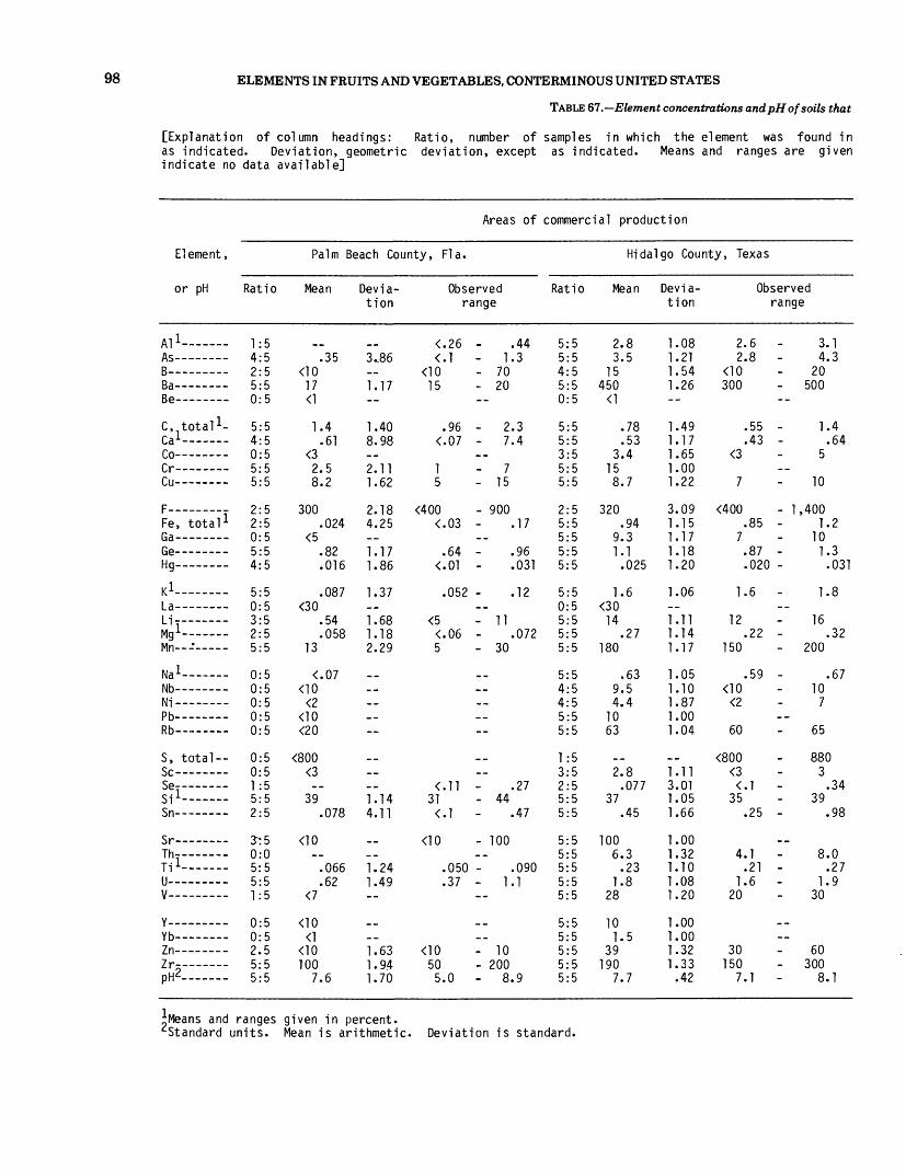
98 ELEMENTS IN FRUITS AND VEGETABLES, CONTERMINOUS UNITED STATES
TABLE 67.—Element concentrations and pH of soils that
[Explanation of column headings: Ratio, number of samples in which the element was found in as indicated. Deviation, geometric deviation, except as indicated. Means and ranges are given indicate no data available]
Element,
or pH
All————
Be —————
C, total 1-
Co —————
Cu —— - —
Fe, total 1 Ga —————
Hg—- ....
K lLa —————Li — ———
Mn— -* ———
Nb —————Ni— ———Pb —————
S, total-- Sc —————
o -1
Sn —————
sr _ _ _____Tn— ———Til —— ___U ——————V ——————
Y ——————V W
Zn —————Zr —————PS?---
Areas of commercial production
Palm Beach County, Fla.
Ratio
1:5 4:5 2:5 5:5 0:5
5:5 4:5 0:5 5:5 5:5
2:5 2:5 0:5 5:5 4:5
5:5 0:5 3:5 2:5 5:5
0:5 0:5 0:5 0:5 0:5
0:5 0:5 1:5 5:5 2:5
3^5 0:0 5:5 5:5 1:5
0:5 0:5 2.5 5:5 5:5
Mean
.35
17
1.4 .61
<3 2.5 8.2
300 .024
<5 .82 .016
.087 <30
.54
.058 13
<.07
<2
<20
<800 <3
39 .078
.066
.62 <7
100 7.6
Devia tion
3.86
1.17
1.40 8.98
2.11 1.62
2.18 4.25
1.17 1.86
1.37
1.68 1.18 2.29
1.14 4.11
1.24 1.49
1.63 1.94 1.70
<. <.
<10 15
<.
1 5
<400 <.
<5 <.5
31*
<10
<10 50 5.
Observed range
26 - .44 1 - 1.3
- 70 - 20
96 - 2.3 07 - 7.4
- 7 - 15
- 900 03 - .17
64 - .96 01 - .031
052 - .12
- 11 06 - .072
- 30
11 - .27 - 44
1 - .47
- 100
050 - .090 37 - 1.1
- 10 - 200
0 - 8.9
Ratio
5:5 5:5 4:5 5:5 0:5
5:5 5:5 3:5 5:5 5:5
2:5 5:5 5:5 5:5 5:5
5:5 0:5 5:5 5:5 5:5
5:5 4:5 4:5 5:5 5:5
1:5 3:5 2:5 5:5 5:5
5:5 5:5 5:5 5:5 5:5
5:5 5:5 5:5 5:5 5:5
Hidalgo County, Texas
Mean
2.8 3.5
15 450
.78
.53 3.4
15 8.7
320 .94
9.3 1.1 .025
1.6 <30 14
.27 180
.63 9.5 4.4
10 63
2.8 .077
37 .45
100 6.3 .23
1.8 28
10 1.5
39 190
7.7
Devia tion
1.08 1.21 1.54 1.26
1.49 1.17 1.65 1.00 1.22
3.09 1.15 1.17 1.18 1.20
1.06
1.11 1.14 1.17
1.05 1.10 1.87 1.00 1.04
1.11 3.01 1.05 1.66
1.00 1.32 1.10 1.08 1.20
1.00 1.00 1.32 1.33 .42
2. 2.
300
7
<400 7*
1.
12
150
<2
60
<800 <335*
4.
1. 20
30 150
7.
Observed range
6 - 3.1 8 - 4.3
20 - 500
55 - 1.4 43 - .64
5
10
- 1,400 85 - 1.2
10 87 - 1.3 020 - .031
6 - 1.8
16 22 - .32
- 200
59 - .67 10 7
65
880 3
1 - .34 39
25 - .98
1 - 8.0 21 - .27 6 - 1.9
30
60 - 300
1 - 8.1
^Means and ranges given in percent.^Standard units. Mean is arithmetic. Deviation is standard.

TABLES 4-121
supported grapefruit trees in areas of commercial production
measurable concentrations to number of samples analyzed, in parts per million, except where percent is indicated.
Mean, geometric mean, except Leaders (--) in figure column
99
Areas of commercial production (continued)
Riverside County, Calif.
Ratio
5:55:50:55:55:5
5:55:55:55:55:5
5:55:55:55:55:5
5:55:55:55:55:5
5:55:55:55:55:5
2:55:50:55:55:5
5:55:55:55:55:5
5:55:55:55:55:5
Mean
6.83.2
<101,100
1.2
.623.08.1
2615
8702.6
201.3
.018
2.45728
1.1480
2.6101316
110
7309.4<.l
281.6
66015
.402.6
88
282.8
76180
8.6
Devia tion
1.051.21--1.201.25
1.251.061.221.501.28
1.171.081.281.131.53
1.001.361.091.081.35
1.021.001.251.141.10
1.811.37__1.032.78
1.461.261.091.131.40
1.201.201.111.50
.19
Observed range
6.42.6
1,0001.0
.482.77
2010
7002.4
151.1.010
5025
1.0300
2.5
101590
<8007
27.79
50011
.362.3
70
202
66100
8.4
7.24.2
_-- 1,500
1.5
.843.2
105020
- 1,0003.0
301.5
.030
__100
311.2
- 700
2.7__
1520
- 120
- 1,43015
__299.6
- 1,00021
.443.2
- 150
308
88- 300
8.9
Ratio
5:55:54:55:54:5
5:55:55:55:55:5
5:55:55:55:55:5
5:55:55:55:55:5
5:53:55:55:55:5
0:55:53:55:55:5
5:55:55:55:55:5
5:55:55:55:55:5
Yuma County, Ariz.
Mean
5.95.4
141,300
.95
.823.38.1
7019
6102.5
161.3
.029
2.538271.0
440
1.78.9
191895
<8009.3
.1229
.82
7009.2
.382.6
93
192.0
67230
8.8
Devia tion
1.091.201.501.251.10
1.391.111.221.281.33
1.391.061.141.151.19
1.061.711.071.091.44
1.101.161.331.171.05
__1.171.651.021.56
1.411.311.051.081.17
1.331.461.081.67.36
Observed range
5.44.3
<101,000
<1
.572.97
5015
4002.4
151.1
.024
2.33025
.92300
1.5<10
151590
7<.l
28.46
5006.8
.35
.2470
151.5
60150
8.5
6.77.2
20- 1,500
1
1.33.8
10100
30
- 9002.7
201.6
.037
2.7100
291.1
700
1.9103020
- 100
__10
.2330
1.2
- 1,00014
.392.9
100
303.0
73- 500
9.3
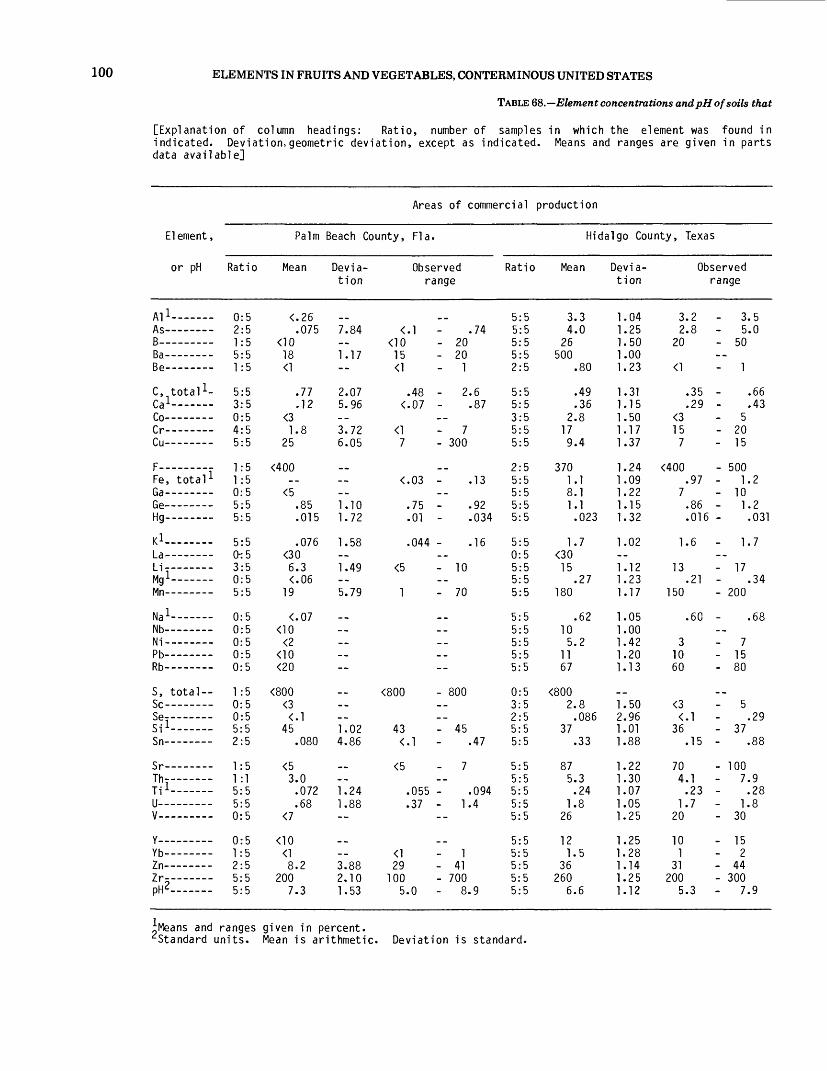
100 ELEMENTS IN FRUITS AND VEGETABLES, CONTERMINOUS UNITED STATES
TABLE 68.—Element concentrations and pH of soils that
[Explanation of column headings: Ratio, number of samples in which the element was found in indicated. Deviation,geometric deviation, except as indicated. Means and ranges are given in parts data available]
Areas of commercial production
Element,
or pH
All————
D ̂
C, total 1 -
Co --------f r--------Cu --------
Fe, total 1 Ga— ———Ge --------Hg— ———
La——— —Li —————Mg 1 — — —
lNb- — — _Ni — ___—Pb _——___Rb —— - — —
S, total —_c^lSi 1 _-— —Sn — — —
Th— - ——Til-— —u _________V _______
Y ——————vu
Zn— —— —
pH2 ————
Palm Beach County, Fla.
Ratio
0:5 2:5 1:5 5:5 1:5
5:5 3:5 0:5 4:5 5:5
1:5 1:5 0:5 5:5 5:5
5:5 0-:5 3:5 0:5 5:5
0:5 0:5 0:5 0:5 0:5
1:5 0:5 0:5 5:5 2:5
1:5 1:15:5 5:5 0:5
0:5 1:5 2:5 5:5 5:5
Mean
<.26 .075
18
.77
.12 <3 1.8
25
<400
<5.85 .015
.076 <30 6.3 <.06
19
<.07
<2
<20
<800 <345*
.080
<5 3.0 .072 .68
<7
8.2 200
7.3
Devia tion
7.84
1.17
2.07 5.96
3.72 6.05
1.10 1.72
1.58
1.49
5.79
1.02 4.86
1.24 1.88
3.88 2.10 1.53
Observed range
<.l - .74 <10 - 20 15 - 20 <1 - 1
.48 - 2.6 <.07 - .87
<1 - 7 7 - 300
<.03 - .13
.75 - .92
.01 - .034
.044 - .16
<5 - 10
1 - 70
<800 - 800
43 - 45 <.l - .47
<5 - 7
.055 - .094
.37 - 1.4
<1 - 1 29 - 41 100 - 700
5.0 - 8.9
Ratio
5:5 5:5 5:5 5:5 2:5
5:5 5:5 3:5 5:5 5:5
2:55:5 5:5 5:5 5:5
5:5 0:5 5:5 5:5 5:5
5:5 5:5 5:5 5:5 5:5
0:5 3:5 2:5 5:5 5:5
5:5 5:5 5:5 5:5 5:5
5:5 5:5 5:5 5:5 5:5
Hidalgo County, Texas
Mean
3.3 4.0
26 500
.80
.49
.36 2.8
17 9.4
370 1.1 8.1 1.1 .023
1.7 <30 15
.27 180
.62 10 5.2
11 67
<800 2.8 .086
37 .33
87 5.3 .24
1.8 26
12 1.5
36 260
6.6
Devia tion
1.04 1.25 1.50 1.00 1.23
1.31 1.15 1.50 1.17 1.37
1.24 1.09 1.22 1.15 1.32
1.02
1.12 1.23 1.17
1.05 1.00 1.42 1.20 1.13
1.50 2.96 1.01 1.88
1.22 1.30 1.07 1.05 1.25
1.25 1.28 1.14 1.25 1.12
Observed range
3.2 2.8
20
.35
.29 <3 15 7
<400 .97
7 .86 .016
1.6
13 .21
150
.60
3 10 60
<336*
.15
70 4.1 .23
1.7 20
10 1
31 200
5.3
- 3.5 - 5.0 - 50
- 1
.66
.43 - 5 - 20 - 15
- 500 - 1.2 - 10 - 1.2
.031
- 1.7
- 17 .34
- 200
.68
- 7 - 15 - 80
- 5 .29
- 37 .88
- 100 7.9 .28
1.8 - 30
- 15 - 2 - 44 - 300 - 7.9
*Means and ranges given in percent.^Standard units. Mean is arithmetic. Deviation is standard.

TABLES 4-121
supported orange trees in areas of commercial production
measurable concentrations to number of samples analyzed. Mean, geometric mean, except as per million, except where percent is indicated. Leaders (--) in figure column indicate no
101
Areas of commercial production (continued)
Riverside County, Calif.
Ratio
5:55:50:55:55:5
5:55:55:55:55:5
5:55:55:55:55:5
5:54:55:55:55:5
5:54:55:55:55:5
1:55:51:55:55:5
5:55:55:55:55:5
5:55:55:55:55:5
Mean
6.62.4
<101,300
1.1
.482.77
318.8
6902.1
191.2.032
2.45519
.80330
2.69.5
1317
100
<8007--
30.69
61015
.342.3
65
171.7
59160
8.6
Devia tion
1.071.70--1.251.20
1.361.051.001.381.40
1.261.061.141.171.51
1.012.441.091.101.58
1.041.101.251.171.04
__1.00--1.071.19
1.201.161.071.091.16
1.171.171.211.49
.52
Observed range
6.01.1
1,0001
.322.5
207
5002.0
15.94.019
2.3<30
17.69
200
2.5<10
101595
<800
<.l27
.53
50013
.322.0
50
151.5
48100
8.0
7'.2
4.6_-- 1,500
1.5
.702.8
__5015
- 9002.3
201.4.059
2.4150
21.88
700
2.7101520
- 105
- 960--
.2532
.82
- 70019
.382.6
70
202
80- 300
9.3
Ratio
4:55:54:55:55:5
5:55:55:55:55:5
5:54:55:55:55:5
5:53:55:55:55:5
5:53:55:55:55:5
0:55:53:55:55:5
5:55:55:55:55:5
5:55:55:55:55:5
Yuma County, Ariz.
Mean
2.63.0
151,100
1.0
.771.68.1
6614
500.90
16.90.029
1.328
19.75
330
1.28.9
211767
<8008.1
.1331
.68
61011
.262.4
93
161.7
53160
8.8
Devia tion
4.601.881.541.201.00
1.235.241.221.331.35
1.158.281.141.731.18
4.421.112.111.911.26
1.931.161.421.171.98
__1.222.181.161.50
1.361.132.211.041.17
1.491.361.431.14.15
Observed range
<.261.2
<101,000
.57
.0817
5010
400<.03
15.34.024
.092<30
5.24
300
.39<10
151520
7<.l
29.50
5009.9
.0622.3
70
101.5
28150
8.6
6.14.9
20- 1,500--
1.03.7
10100
20
- 6002.6
201.2
.035
2.83029
1.1- 500
1.9103020
100
__10
.3140
1.3
- 1,00013
.392.5
- 100
303
67- 200
9.0

102 ELEMENTS IN FRUITS AND VEGETABLES, CONTERMINOUS UNITED STATES
TABLE 69.—Element concentrations and pH of soils that
[Explanation of column headings: Ratio, number of samples in which the element was found in indicated. Deviation, geometric deviation, except as indicated. Means and ranges are given in parts no data available]
Areas of commercial production
El ement ,
or pH
Al 1-Ac
O-,
Be —— — -
C, total 1 - ral- _ _ _Co —————Pr__Cu— — --
Fe, total 1 Ga —————Ge— — -Hg— — -
K!La —————U ........Mn —————
Nal-- -_-Mb —————Ni —————Pb —————Rb —————
S, total-- Sc _____Se_ ____Si —————Sn ———— -
sr_ _ _____Th_ _ _ ___in - Til- — ——U ——————V ——————
Y ——————WL
Zn —————Zr ————pH2~~~
Ratio
5:5 5:5 .4:5 5:5 0:5
5:5 5:5 5:5 5:5 5:5
3:5 5:5 5:5 5:5 5:5
5:5 1:5 5:5 5:5 5:5
5:5 3:5 5:5 5:5 5:5
2:55:5 1:5 5:5 5:5
5:5 5:5 5:5 5:5 5:5
5:5 5:5 5:5 5:5 5:5
Wayne County
Mean Devia tion
4.0 24 17
390 <1
2.7 .63
5.3 26 19
460 1.9
14 1.3
.059
1.4 <30
21 .39
300
1.0 8.9 9.4
90 49
770 5.3 <.l
33 .69
150 5.6
.40 2.0
45
16 2.0
63 260
5.5
1.11 4.16 1.70 1.48
1.16 1.10 1.16 1.25 1.33
1.26 1.11 1.20 1.12 1.32
1.05
1.19 1.15 1.72
1.06 1.16 1.37 2.88 1.23
1.25 1.16
1.04 2.51
1.30 1.49 1.13 1.03 1.26
1.33 1.46 1.18 1.50 .53
, N.Y.
Observed range
3.6 2.6
<10 300
2.1 .56
5 20 15
<400 1.7
10 1.0
.040
1.4 <30
17 .34
150
.98 <10
7 20 40
<800 5 <.l
31 .15
100 3.3
.34 1.9
30
10 1.5
53 200
4.9
4. - 110
30 - 700
3.7*
30 30
- 600 2.
15 1.
1. 30 25
- 500
1. 10 15
- 300 65
- 1,000 7
35 1.
- 200 9.
2.50
20 3.
78 - 500
6.
6
1 73
2
4 085
5
46
1
16
6
5 461
0
0
Ratio
5:5 5:5 1:5 5:5 3:5
5:5 5:5 5:5 5:5 5:5
5:5 5:5 5:5 5:5 5:5
5:5 1:5 5:5 5:5 5:5
5:5 4:5 5:5 5:5 5:5
5:5 5:5 3:5 5:5 4:5
5:5 5:5 5:5 5:5 5:5
5:5 5:5 5:5 5:5 5:5
Yakima
Mean
6.7 2.9
<10 530
.89
1.6 3.0
14 57 36
480 4.3
19 1.3
.043
1.3 <30 22
1.3 500
1.9 9.5
25 11 50
1,900 15
.11 27
.71
450 8.9
.63 2.1
150
17 1.9
82 150
5.7
County
Devia tion
1.06 1.27
1.16 1.16
1.08 1.06 1.20 1.36 1.46
1.10 1.02 1.14 1.18 1.31
1.05
1.03 1.03 1.00
1.00 1.10 1.60 1.20 1.07
1.81 1.00 1.65 1.03 3.63
1.26 1.13 1.02 1.07 1.00
1.17 1.14 1.04 1.28 .86
, Wash.
Observed range
6.1 2.3
<10 500
<1
1.5 2.7
10 50 30
400 4.2
15 1.0
.032
1.2 <30
21 1.2
<10 15 10 45
940
<.l 21 <.l
300 7.5
.61 1.9
15 1.5
77 100
4.3
7.03 3.8
20 - 700
1
1.8 3.2
15 - 100
70
- 500 4.4
20 1.5
.063
1.4 70 23
1.3
10 50 15 55
- 4,100
.22 28
1.5
- 500 9.9
.65 2.3
20 2.0
86 - 200
6.4
^Means and ranges given in percent.^Standard units. Mean is arithmetic. Deviation is standard.
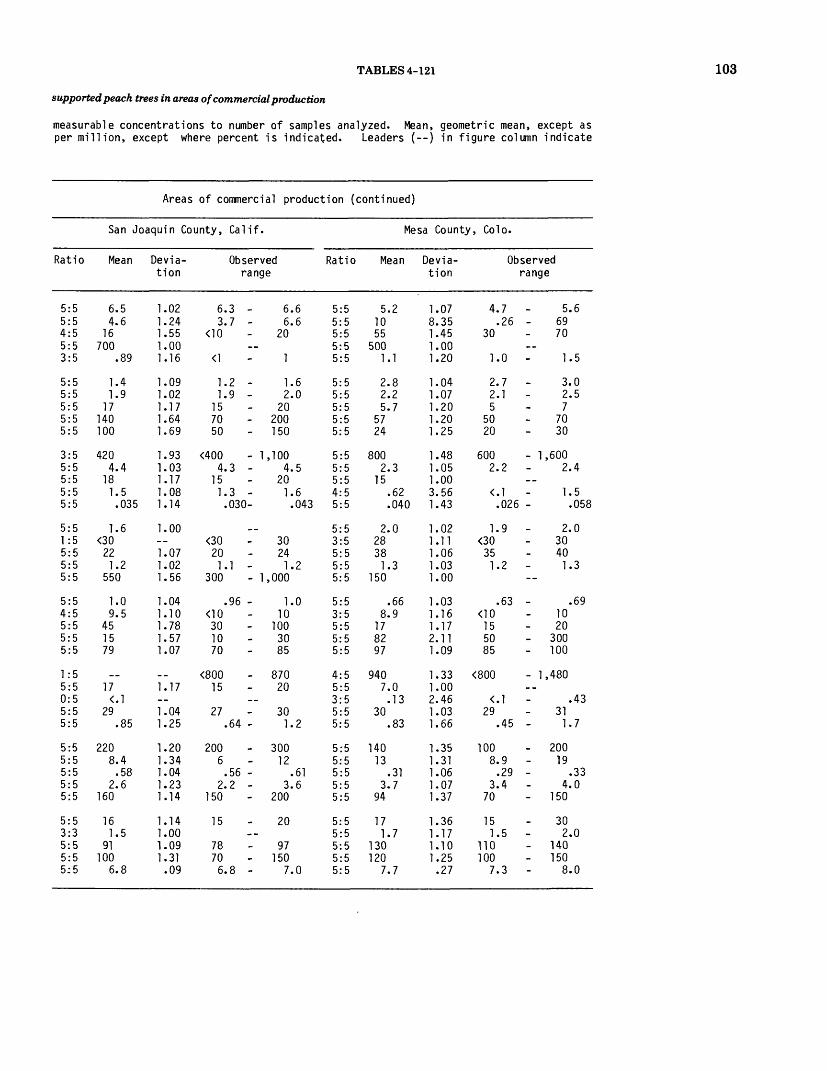
TABLES 4-121
supported peach trees in areas of commercial production
measurable concentrations to number of samples analyzed. Mean, geometric mean, except as per million, except where percent is indicated. Leaders (--) in figure column indicate
103
Areas of commercial production (continued)
San Joaquin County, Calif.
Ratio
5:55:54:55:53:5
5:55:55:55:55:5
3:55:55:55:55:5
5:51:55:55:55:5
5:54:55:55:55:5
1:55:50:55:55:5
5:55:55:55:55:5
5:53:35:55:55:5
Mean
6,54.6
16700
.89
1.41.9
17140100
4204.4
181.5.035
1.6<30221.2
550
1.09.5
451579
_17<.l
29.85
2208.4.58
2.6160
161.5
91100
6.8
Devia tion
1.021.241.551.001.16
1.091.021.171.641.69
1.931.031.171.081.14
1.00--1.071.021.56
1.041.101.781.571.07
__1.17—1.041.25
1.201.341.041.231.14
1.141.001.091.31.09
Observed range
6.3 -3.7 -
<10._
<1
1.2 -1.9 -
157050
<400 - 14.3 -
151.3 -.030-
__<30201.1 -
300 - 1
.96 -<10301070
<80015
__27
.64 -
2006.56 -
2.2 -150
15_-
78706.8 -
6.66.6
20
1
1.62.0
20200150
,1004.5
201.6.043
30241.2
,000
1.010
1003085
87020
301.2
30012
.613.6
200
20
97150
7.0
Ratio
5:55:55:55:55:5
5:55:55:55:55:5
5:55:55:54:55:5
5:53:55:55:55:5
5:53:55:55:55:5
4:55:53:55:55:5
5:55:55:55:55:5
5:55:55:55:55:5
Mesa County, Colo.
Mean Devia tion
5.21055500
1.1
2.82.25.7
5724
8002.3
15.62.040
2.028381.3
150
.668.9
178297
9407.0.13
30.83
14013
.313.7
94
171.7
130120
7.7
1.078.351.451.001.20
1.041.071.201.201.25
1.481.051.003.561.43
1.021.111.061.031.00
1.031.161.172.111.09
1.331.002.461.031.66
1.351.311.061.071.37
1.361.171.101.25.27
Observed range
4.7.26
30
1.0
2.72.15
5020
6002.2
<.l.026
1.9<30351.2
.63<10155085
<800
<.l29
.45
1008.9.29
3.470
151.5
110100
7.3
5.66970
__1.5
3.02.57
7030
- 1,6002.4
--1.5.058
2.030401.3
--
.691020
- 300- 100
- 1,480--
.43311.7
- 20019
.334.0
- 150
302.0
- 140- 150
8.0

104 ELEMENTS IN FRUITS AND VEGETABLES, CONTERMINOUS UNITED STATES
TABLE 70.—Element concentrations and pH of soils that
[Explanation of column headings: Ratio, number of samples in which the element was found in except as indicated. Means and ranges are given in parts per million, except where percent is
Areas of commercial production
El ement ,
or pH
All————
D -i
Be __— —
C.-total 1 - (-•,1Co — _— —
Fe, total 1 Ga — — _-Ge — — —Hg— ———
K 1 -La — — —
Mgl _______
Na 1Mb — — —Ni _____ ___Pb _ — _—__Rb ________
S, total —_SI 1-- — -Sn — — —
Th-— ——Til- — __.u _________V _______
Y _________
Zn ——— —Zr-~- ——pH2— ——
Bern en County, Mich.
Ratio
5:5 5:5 5:5 5:5 1:5
5:5 5:5 4:5 5:5 5:5
0:5 5:5 5:5 5:5 5:5
5:5 0:5 5:5 5:5 5:5
5:5 4:5 5:5 5:5 5:5
0:5 4:5 3:5 5:5 5:5
5:5 4:4 5:5 5:5 5:5
5:5 5:5 5:5 5:5 5:5
Mean
3.15.8
38 450
1.2 .33
5.1 24 25
<400 1.4 8.8 1.3 .044
1.7 <30 17
.25 460
.65 9.5
10 20 66
<800 4 .12
36 .59
75 7.1 .28
1.8 40
12 1.4
53 190
5.4
Devia tion
1.26 1.66 1.52 1.26
.30
.11
.62
.37
.68
1.34 1.51 1.19 1.51
1.16
1.55 1.46 1.91
1.47 1.10 1.69 1.28 1.26
1.61 1.69 1.04 1.59
1.17 1.41 1.31 1.15 1.64
1.25 1.42 1.17 1.33 .74
Observed range
2.2 2.8
20 300
.84
.29 <3 15 15
1.0 5 1.0 .031
1.4
10 .16
200
.53
5 15 50
<333*
.35
70 5.2 .19
1.5 20
10 1
40 150
4.5
3.9 9.2
50 - 500
1
1.7 .38
7 30 50
1.9 15 1.6 .078
2.0
26 .37
- 1,000
1.3 10 15 30 85
7 .22
37 1.2
- 100 11
.39 2.1
70
15 2
60 - 300
6.2
Ratio
5:5 5:5 5:5 5:5 1:5
5:5 5:5 5:5 5:5 5:5
3:5 5:5 5:5 5:5 5:5
5:5 1:5 5:5 5:5 5:5
5:5 5:5 5:5 5:5 5:5
0:5 5:5 1:5 5:5 4:5
5:5 4:4 5:5 5:5 5:5
5:5 5:5 5:5 5:5 5:5
Wayne County
Mean
4.3 7.0
28 340
2.0 .68
5.9 27 13
420 2.0
12 1.2 .060
1.5 <30 29
.49 360
1.0 10 12 23 55
<800 5.5
34 .56
140 7.7 .45
2.2 44
18 1.9
60 210
6.6
Devia tion
1.16 3.19 1.46 1.48
.29
.72
.57
.58
.58
1.32 1.30 1.25 1.24 1.33
1.16
1.22 1.27 2.25
1.15 1.00 1.62 2.10 1.50
1.56
1.04 3.23
1.35 1.20 1.13 1.17 1.44
1.50 1.49 1.49 1.86 .87
, N.
3 1
20 200
1
3 15 7
<400 1
10
1 <30 21
150
7 10 30
3
33
100 6
1 30
10 1
31 100
5
Y.
Observed range
.6 - 4.9
.1 - 24 50
- 500 1
.4 - 2.7
.36 - 1.2 10 50 20
- 600 .3 - 2.5
15 .87 - 1.5 .047 - .096
.2 - 1.7 30 34
.36 - .63 - 1,000
.87 - 1.2
20 70 85
10 .1 - .21
36
- 200 .0 - 9.3 .37 - .50 .8 - 2.6
70
30 3
90 - 500
.7 - 7.8
^Means and ranges given in percent.^Standard units. Mean is arithmetic. Deviation is standard.

TABLES 4-121 105supported pear trees in areas of commercial production
measurable concentrations to number of samples analyzed. Mean, geometric mean, except as indicated. Deviation, geometric deviation indicated. Leaders (—) in figure column indicate no data available.]
Areas of commercial production (continued)
Yakima County, Wash. San Joaquin County, Calif. Mesa County, Colo.
Ratio
5:55:51:55:55:5
5:55:55:55:55:5
5:55:55:55:55:5
5:53:55:55r55:5
5:51:55:55:55:5
2:55:52:55:55:5
5:55:55:55:55:5
5:55:55:55:55:5
Mean
6.323—
5701.1
2.41.9
125744
6903.1
191.0
.029
1.62823
1.1370
1.7<10
19160
58
77015
.08329
.84
4508.2
.492.0
130
202.0
160no
6.3
Devia tion
1.351.35--1.201.20
1.172.181.251.201.44
1.531.671.141.261.36
1.051.111.141.041.32
1.04—1.141.331.08
1.241.002.761.141.24
1.261.171.291.061.25
1.281.281.171.20
.31
Observed range
3.714
<10500
1.0
1.8.47
105030
4001.2
15.71.019
1.5<3020
1.1300
1.7<10
15100
55
<800
<.l27
.68
3007.0
.311.8
100
151.5
140100
6.0
7.42915
- 7001.5
2.82.8
157070
- 1,2004.0
201.2.040
1.73028
1.2- 500
1.81020
- 20065
- 900-_
.3136
1.2
- 50011
.562.1
- 150
303
- 210- 150
6.7
Ratio
5:55:54:55:55:5
5:55:55:55:55:5
5:55:55:55:55:5
5:51:55:55:55:5
5:54:55:55:55:5
1:55:53:55:55:5
5:55:55:55:55:5
5:54:45:55:55:5
Mean
7.51419
8701.0
2.61.8
17110240
5704.9
201.4
.073
1.8<30
271.4
600
.999.5
656193
_19
.1625
1.1
2409.9
.542.7
170
202.0
12095
7.0
Devia tion
.08
.15
.81
.22
.00
1.171.101.171.361.37
1.201.041.001.161.30
1.03—1.071.011.68
1.031.101.891.201.21
__1.142.581.031.23
.25
.44
.03
.08
.17
.28
.331.061.525.96
Observed range
6.712
<10700
2.21.7
15100150
5004.7
1.2.057
1.7<30
251.3
300
.95<10305070
<80015<.l
24.90
2006.3
.522.5
150
151.5
120706.5
8.01630
- 1,000--
3.32.2
20- 200- 300
- 7005.1
_1.7
.10
1.83030
1.4- 1,000
1.010
- 15070
- 110
- 86020
.3526
1.5
- 30015
.563.1
- 200
303.0
- 130- 150
8.0
Ratio
5:55:55:55:55:5
5:55:55:55:55:5
5:55:55:55:55:5
5:52:55:55:55:5
5:51:55:55:55:5
0:55:52:55:55:5
5:55:55:55:55:5
5:55:55:55:55:5
Mean
4.69.1
28610
1.2
2.94.56.1
4828
6602.5
151.1
.042
1.926281.0
230
.74<10
142884
<8007.0<.l
281.0
24013
.303.4
75
151.4
85140
8.0
Devia tion
.13
.18
.20
.36
.63
1.201.251.201.352.11
1.301.071.001.212.47
1.111.161.121.081.58
1.04._1.201.201.17
__1.00—1.041.26
1.251.241.071.051.17
1.001.201.091.351.30
Observed range
4.07.4
20500
1
2.33.65
3015
5002.4
.80
.019
1.6<30
25.94
150
.70<10
102065 •
27.70
20010
.273.2
70
1.076
1007.8
5.41130
- 1,0003
3.86.57
70- 100
- 1,0002.7
__1.3
.20
2.030331.2
- 500
.7710153095
__—-_
301.3
- 30018
.323.6
- 100
__1.5
94- 200
8.1
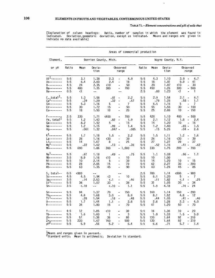
106 ELEMENTS IN FRUITS AND VEGETABLES, CONTERMINOUS UNITED STATES
TABLE 71.—Element concentrations and pH of soils that
[Explanation of column headings: Ratio, number of samples in which the element was found in indicated. Deviation,geometric deviation, except as indicated. Means and ranges are given in indicate no data available]
Element,
or pH
All-——n<- _ ______
Ra
Be———— -
C.-total 1 -r-,l__ _ ___Co- — ——o_____ _ _Cu —————
F—— ...Fe, total 1 Ga— ———Ge——— —Hg— -----
K 1La-- ———Li ——— —Mg 1 ————Mn —————
Mal_
Mb ———— -Ni —————Pb —— — -Rb —————
S, total-- Sc_ _ _ _ __Se ____ -i Si 1 ————Sn —————
sr _ _ _ ___Th——— ——Til —————U ——————V— ————
Y ——————WL
Zn —————z r ———J,2pH —————
Areas of commercial production
Berrien County, Mich.
Ratio
5:5 5:5 4:5 5:5 0:5
5:5 5:5 5:5 5:5 5:5
2:5 5:5 5:5 5:5 5:5
5:5 2:5 5:5 5:5 5:5
5:5 3:5 5:5 5:5 5:5
0:5 4:5 3:5 5:5 3:5
5:5 5:5 5:5 5:5 5:5
4:5 5:5 5:5 5:5 5:5
Mean
3.1 6.4
24 480 <1
1.3 .39
5.3 30 18
330 1.2 8.2 1.2 .061
1.7 26 14
.22 690
.61 8.9 10 28 63
<800 4.5 .14
36 <.10
94 4.8 .28
1.7 34
12 1.6
57 230
5.9
Devia tion
1.38 2.60 2.35 1.35
1.58 1.29 1.16 1.72 1.50
1.71 1.43 1.52 1.15 1.32
1.18 1.16 1.67 1.62 1.86
1.18 1.16 2.14 2.05 1.35
1.94 2.53 1.07
1.37 1.68 1.54 1.44 1.80
1.85 1.60 1.38 1.67 .56
Observed range
2.3 2.4
<10 300
.81
.32 5
15 10
<400 .82
5 .99 .047
1.5 <30
8 .13
300
.49 <10
5 15 45
<3 <.l
33 <.10
70 3.0 .18
1.1 15
<10 1
38 150
5.2
4.9 18 50
- 700
2.2 .57
7 50 20
- 700 1.9
15 1.4 .085
2.2 30 25
.36 - 1,500
.75 10 30 70 90
10 .46
38 1.1
- 150 8.9 .48
2.8 70
30 3
80 - 500
6.4
Ratio
5:5 5:5 4:5 5:5 2:5
5:5 5:5 5:5 5:5 5:5
5:5 5:5 5:5 5:5 5:5
5:5 2:5 5:5 5:5 5:5
5:5 5:5 5:5 5:5 5:5
2:5 5:5 3:5 5:5 5:5
5:5 5:5 5:5 5:5 5:5
5:5 5:5 5:5 5:5 5:5
Wayne County, N.Y.
Mean
4.3 18 20
450 .80
2.9 .79
6.5 55 25
420 2.1
14 1.2 .15
1.5 26 27
.52 330
1.1 10 14 62 63
780 6.1 .11
31 1.9
160 8.1 .44
2.8 61
16 1.9
130 130
6.6
Devia tion
1.10 1.81 1.87 1.26 1.23
1.54 1.26 1.16 1.56 2.86
1.10 1.12 1.20 1.40 5.26
1.11 1.16 1.27 1.16 1.75
1.08 1.00 1.20 2.27 1.26
1.14 1.20 1.82 1.05 4.18
1.14 1.52 1.05 1.28 1.20
1.36 1.33 1.64 1.64 .71
Observed range
3.9 9.9
<10 300 <1
2.1 .58
5 30 10
400 1.8
10 .65 .04
1.2 <30 20
.41 200
.96
10 30 45
<800 5 <.l
30 .74
150 4.8 .41
2.3 50
10 1.5
92 92 5.7
- 4.7 - 41 - 30 - 500 - 1
- 6.1 - 1.1 - 7 - 100 - 150
- 500 - 2.4 - 15 - 1.5 - 2.6
- 1.6 - 30 - 37
.62 - 700
- 1.1
- 15 - 200 - 85
- 900 - 7
.25 - 34 - 24
- 200 - 12
.46 - 4.0 - 70
- 20 - 3.0 - 310 - 310 - 7.4
gleans and ranges given in percent.^Standard units. Mean is arithmetic. Deviation is standard.
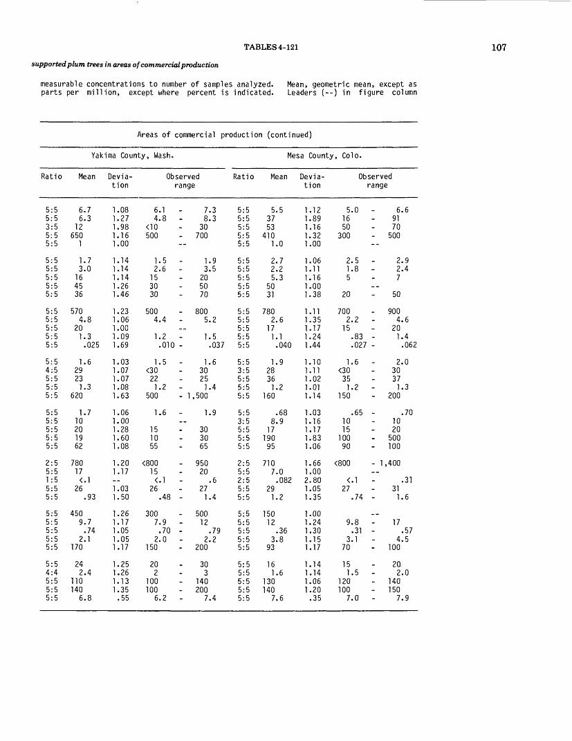
TABLES 4-121 107
supported plum trees in areas of commercial production
measurable concentrations to number of samples analyzed. Mean, geometric mean, except as parts per million, except where percent is indicated. Leaders (--) in figure column
Areas of commercial production (continued)
Yakima County, Wash.
Ratio
5:55:53:55:55:5
5:55:55:55:55:5
5:55:55:55:55:5
5:54:55:55:55:5
5:55:55:55:55:5
2:55:51:55:55:5
5:55:55:55:55:5
5:54:45:55:55:5
Mean
6.76.3
12650
1
1.73.0
164536
5704.8
201.3
.025
1.629231.3
620
1.710201962
78017<.l
26.93
4509.7
.742.1
170
242.4
110140
6.8
Devia tion
1.081.271.981.161.00
1.141.141.141.261.46
1.231.061.001.091.69
1.031.071.071.081.63
1.061.001.281.601.08
1.201.17__1.031.50
1.261.171.051.051.17
1.251.261.131.35
.55
Observed range
6.14.8
<10500
1.52.6
153030
5004.4
1.2.010
1.5<30
221.2
500
1.6
151055
<80015<.l
26.48
3007.9.70
2.0150
202
100100
6.2
7.38.3
30- 700--
1.93.5
205070
- 8005.2
__1.5
.037
1.630251.4
- 1,500
1.9__
303065
- 95020
.627
1.4
- 50012
.792.2
- 200
303
- 140- 200
7.4
Ratio
5:55:55:55:55:5
5:55:55:55:55:5
5:55:55:55:55:5
5:53:55:55:55:5
5:53:55:55:55:5
2:55:52:55:55:5
5:55:55:55:55:5
5:55:55:55:55:5
Mesa County, Colo.
Mean
5.53753
4101.0
2.72.25.3
5031
7802.6
171.1
.040
1.928361.2
160
.688.9
17190
95
7107.0
.08229
1.2
15012
.363.8
93
161.6
130140
7.6
Devia tion
1.121.891.161.321.00
1.061.111.161.001.38
1.111.351.171.241.44
1.101.111.021.011.14
1.031.161.171.831.06
1.661.002.801.051.35
1.001.241.301.151.17
1.141.141.061.20
.35
Observed range
5.01650
300
2.51.85
20
7002.2
15.83.027
1.6<30
351.2
150
.651015
10090
<800
<.l27
.74
9.8.31
3.170
151.5
120100
7.0
6.69170
- 500--
2.92.47
__50
- 9004.6
201.4
.062
2.030371.3
- 200
.701020
- 500- 100
- 1,400--
.3131
1.6
__17
.574.5
- 100
20-2.0
- 140- 150
7.9
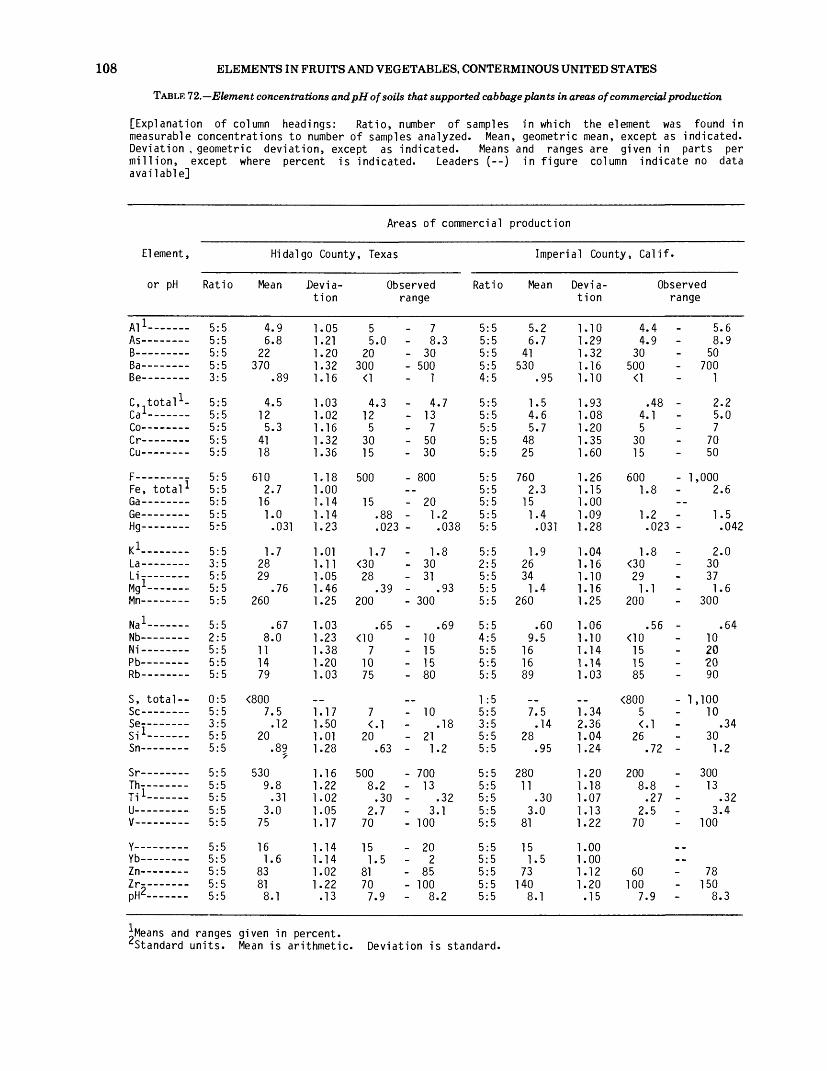
108 ELEMENTS IN FRUITS AND VEGETABLES, CONTERMINOUS UNITED STATES
TABLE 72.—Element concentrations and pH of soils that supported cabbage plants in areas of commercial production
[Explanation of column headings: Ratio, number of samples in which the element was found in measurable concentrations to number of samples analyzed. Mean, geometric mean, except as indicated. Deviation , geometric deviation, except as indicated. Means and ranges are given in parts per million, except where percent is indicated. Leaders (--) in figure column indicate no data available]
Areas of commercial
Element,
or pH
Al 1 -Ac __ ______
R------___D -5
Be— — -
C.-total 1 -r a l_
Co— ———Tr--------Cu —————
F— — ...Fe, total 1 Ga — — —Ge — — —Hg— — -
K 1La .--—__Li _______Mg 1 — __.__Mn — — — _
Na 1Nb —— — ——Ni _______Pb —— —— —Rh--__ _ -
S, total — Sc —————Se — - __ -
i Si 1-——c«
Sr------ _Th— .....Til— — -U ——___.V ——————
Y ________Yb — ———Zn — — —Zr --------J,2pH —— —— -
Ratio
5:5 5:5 5:5 5:5 3:5
5:5 5:5 5:5 5:5 5:5
5:5 5:5 5:5 5:5 5:5
5:5 3:5 5:5 5:5 5:5
5:5 2:5 5:5 5:5 5:5
0:5 5:5 3:5 5:5 5:5
5:5 5:5 5:5 5:5 5:5
5:5 5:5 5:5 5:5 5:5
Hidalgo County , Texas
Mean Devia tion
4.9 6.8
22 370
.89
4.5 12 5.3
41 18
610 2.7
16 1.0 .031
1.7 28 29
.76 260
.67 8.0
11 14 79
<800 7.5 .12
20.89 ?
530 9.8 .31
3.0 75
16 1.6
83 81 8.1
1.05 1.21 1.20 1.32 1.16
1.03 1.02 1.16 1.32 1.36
1.18 1.00 1.14 1.14 1.23
1.01 1.11 1.05 1.46 1.25
1.03 1.23 1.38 1.20 1.03
1.17 1.50 1.01 1.28
1.16 1.22 1.02 1.05 1.17
1.14 1.14 1.02 1.22 .13
5 5.
20 300 <1
4. 12 5
30 15
500
15
1.<30 28
200
<io"7
10 75
7 <.
20
500 8.
2.70
15 1.
81 70 7.
Observed range
- 7 0 - 8.3
- 30 - 500 - 1
3 - 4.7 - 13 - 7 - 50 - 30
- 800
- 20 88 - 1.2 023 - .038
7 - 1.8 - 30 - 31
39 - .93 - 300
65 - .69 - 10 - 15 - 15 - 80
- 10 1 - .18
- 21 63 - 1.2
- 700 2 - 13 30 - .32 7 - 3.1
- 100
- 20 5 - 2
- 85 - 100
9 - 8.2
Ratio
5:5 5:5 5:5 5:5 4:5
5:5 5:5 5:5 5:5 5:5
5:5 5:5 5:5 5:5 5:5
5:5 2:5 5:5 5:5 5:5
5:5 4:5 5:5 5:5 5:5
1:5 5:5 3:5 5:5 5:5
5:5 5:5 5:5 5:5 5:5
5:5 5:5 5:5 5:5 5:5
production
Imperial County
Mean
5.2 6.7
41 530
.95
1.5 4.6 5.7
48 25
760 2.3
15 1.4 .031
1.9 26 34 1.4
260
.60 9.5
16 16 89
7.5 .14
28 .95
280 11
.30 3.0
81
15 1.5
73 140
8.1
Devia tion
, Calif.
1.10 4 1.29 4 1.32 30 1.16 500 1.10 <1
1.93 1.08 4 1.20 5 1.35 30 1.60 15
1.26 600 1.15 1 1.00 1.09 1 1.28
1.04 1 1.16 <30 1.10 29 1.16 1 1.25 200
1.06 1.10 <10 1.14 15 1.14 15 1.03 85
<800 1.34 5 2.36 < 1.04 26 1.24
1.20 200 1.18 8 1.07 1.13 2 1.22 70
1.00 1.00 1.12 60 1.20 100 .15 7
Observed range
.4 - 5.6
.9 - 8.9 50
- 700 1
.48 - 2.2
.1 - 5.0 7
70 50
- 1,000 .8 - 2.6
.2 - 1.5
.023 - .042
.8 - 2.0 30 37
.1 - 1.6 - 300
.56 - .64 10 20 20 90
- 1,100 10
.1 - .34 30
.72 - 1.2
- 300 .8 - 13 .27 - .32 .5 - 3.4
- 100
78 - 150
.9 - 8.3
^Means and ranges given in percent.^Standard units. Mean is arithmetic. Deviation is standard.

TABLES 4-121
TABLE 73.—Element concentrations and pH of soils that supported carrot plants in areas of commercial production
[Explanation of column headings: Ratio, number of samples in which the element was found in measurable concentrations to number of samples analyzed. Mean, geometric mean, except as indicated. Deviation, geometric deviation, except as indicated. Means and ranges are given in parts per million, except where percent is indicated. Leaders (--) in figure column indicate no data available]
109
Areas of commercial production
Element,
or pH
All——.AC;--------
Q-i
Be——— —
C.-total 1 - (-,!_Co—————f r_ _ _____Cu —————
pFe, total 1 Ga— ———Ge——— —Hg— -----
KlLa ——— --Li _____Mg 1 ——————Mn —————
wa l_Nb~ ————Ni —————Pb —————Rb —————
S, total — SC— -----Se--_ ___Si ________Sn -------
Sr- __ - __In-- —— _ -in Til —— ——U —____-_V — ______
Y _________Yb —— — ——Zn —___-_.Zr- ------
0nU^pH —————
Ratio
5:5 5:5. 5:5 5:5 4:5
5:5 5:5 5:5 5:5 5:5
1:5 5:5 5:5 5:5 5:5
5:5 0:5 5:5 5:5 5:5
5:5 4:5 5:5 5:5 5:5
1:5 5:5 1:5 5:5 5:5
5:5 5:5 5:5 5:5 5:5
5:5 5:5 5:5 5:5 5:5
Hidalgo
Mean
4.4 8.0
28 500
.95
1.4 2.5 5
26 15
<400 1.7
13 1.2 .020
2.0 <30 20
.64 240
.67 9.5
10 12 81
5.7
33 .68
150 7.9 .30
2.2 41
14 1.8
52 180
8.1
County
Devia tion
1.09 1.14 1.46 1.00 1.10
1.08 1.14 1.00 1.25 1.00
1.03 1.25 1.10 1.71
1.03
1.13 1.04 1.25
1.05 1.10 1.31 1.25 1.10
1.20
1.02 2.31
1.00 1.23 1.03 1.05 1.32
1.35 1.36 1.06 1.36 .23
, Texas Imperial County
Observed range
3.9 6.8
20
<1
1.2 2.2
20
<400 1.6
10 1.1 .01
1.9
18 .60
200
.63 <10
7 10 75
<800 5 <.l
32 .16
5.8 .29
2.0 30
10 1.5
49 150
7.7
- 5.0 - 9.2 - 50
1
1.5 - 3.0
- 30
- 400 1.7
- 15 - 1.4
.04
- 2.0
- 25 .67
- 300
.72 - 10 - 15 - 15 - 95
- 930 7 .26
- 34 1.3
- 9.8 .31
2.3 - 50
- 20 - 3 - 57 - 300 - 8.3
Ratio
5:5 5:5 5:5 5:5 2:5
5:5 5:5 5:5 5:5 5:5
5:5 5:5 5:5 5:5 4:5
5:5 3:5 5:5 5:5 5:5
5:5 2:5 5:5 5:5 5:5
2:5 5:5 3:5 5:5 5:5
5:5 5:5 5:5 5:5 5:5
5:5 5:5 5:5 5:5 5:5
Mean
5.2 5.9
50 570
.80
1.9 4.4 7
44 30
680 2.3
15 1.3 .019
2.0 28 36 1.4
370
.82 8.0
18 15 87
620 8.7 .14
29 .79
280 9.8 .32
3.1 87
19 1.8
67 130
8.2
Devia tion
, Calif.
Observed range
1.15 4.3 - 1.11 5.3 - 1.00 1.20 500 1.23 <1
1.06 1.7 - 1.23 3.1 - 1.00 1.44 30 1.00
1.07 600 1.09 2.0 - 1.00 1.06 1.2 - 2.03 <.01 -
1.10 1.9 - 1.11 <30 1.06 33 1.07 1.3 - 1.32 300
1.36 68 - 1.23 <10 1.17 15 1.28 10 1.05 80
2.11 <800 - 1 1.22 7 2.07 <.l - 1.04 27 1.57 .39 -
1.20 200 1.17 7.7 - 1.16 .26 - 1.04 2.9 - 1.22 70
1.14 15 1.18 1.5 - 1.04 65 1.25 100 .18 8.0 -
6.2 7.0
700 1
2.0 5.0
70
700 2.6
1.4 .034
2.4 30 38 1.5
500
1.4 10 20 20 90
,800 10
.28 30 1.2
300 11
.40 3.2
100
20 2
72 150
8.4
^Means and ranges given in percent. Standard units, Mean is arithmetic. Deviation is standard.
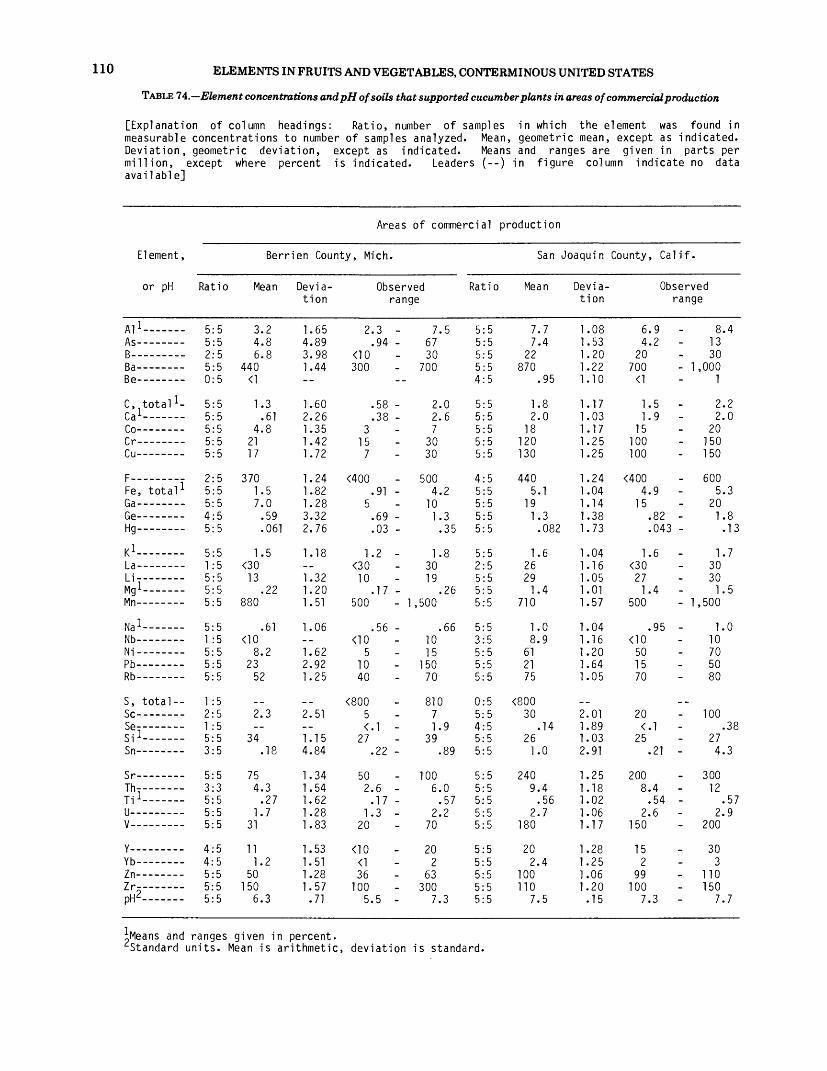
110 ELEMENTS IN FRUITS AND VEGETABLES, CONTERMINOUS UNITED STATES
TABLE 74.—Element concentrations and pH of soils that supported cucumber plants in areas of commercial production
[Explanation of column headings: Ratio, number of samples in which the element was found in measurable concentrations to number of samples analyzed. Mean, geometric mean, except as indicated. Deviation, geometric deviation, except as indicated. Means and ranges are given in parts per million, except where percent is indicated. Leaders (--) in figure column indicate no data available]
Areas of commercial production
Element,
or pH
All — - —As--------
D^
Be--- —— -
C, total 1 -Tal
Co-- ——— --fr--------Cu— —— --
Fe, total 1 Ga--- — --Ge———— -Hg———— -
K 1La ——— —
Mgl ——— ---
Mn —————
Na 1_[\lh________Ni—— ———Pb ——— ---Rb ——— ---
S, total-- Sc— — ---SP--------;>e — ---- Si 1 - _ _Sn —————
Sr- _ ----Th- —— ——Til —————ll_________V _________
y ——————V L.
Zn———— -Zr ——— —J,2pH ———— -
Berrien County, Mich.
Ratio
5:5 5:5 2:5 5:5 0:5
5:5 5:5 5:5 5:5 5:5
2:5 5:5 5:5 4:5 5:5
5:5 1:5 5:5 5:5 5:5
5:5 1 :5 5:5 5:5 5:5
1:5 2:5 1:5 5:5 3:5
5:5 3:3 5:5 5:5 5:5
4:5 4:5 5:5 5:5 5:5
Mean
3.2 4.8 6.8
440 <1
1.3 .61
4.8 21 17
370 1.5 7.0
.59
.061
1.5 <30
13 .22
880
.61 <10
8.2 23
52
2.3
34 .18
75 4.3
.27 1.7
31
11 1.2
50 150
6.3
Devia tion
1.65 4.89 3.98 1.44
1.60 2.26 1.35 1.42 1.72
1.24 1.82 1.28 3.32 2.76
1.18
1.32 1.20 1.51
1.06
1.62 2.92 1.25
2.51
1.15 4.84
1.34 1.54 1.62 1.28 1.83
1.53 1.51 1.28 1.57
.71
Observed range
2.3 .94
<10 300
.58
.38 3
15 7
<400 .91
5 .69 .03
1.2 <30
10 .17
500
.56 <10
5 10 40
<800 5 <.l
27 .22
50 2.6
.17 1.3
20
<10 <1 36
100 5.5
7.5 67 30
- 700
2.0 2.6 7
30 30
- 500 4.2
10 1.3 .35
1.8 30 19
.26 - 1,500
.66 10 15
150 70
810 7 1.9
39 .89
- 100 6.0
.57 2.2
70
20 2
63 - 300
7.3
Ratio
5:5 5:5 5:5 5:5 4:5
5:5 5:5 5:5 5:5 5:5
4:5 5:5 5:5 5:5 5:5
5:5 2:5 5:5 5:5 5:5
5:5 3:5 5:5 5:5 5:5
0:5 5:5 4:5 5:5 5:5
5:5 5:5 5:5 5:5 5:5
5:5 5:5 5:5 5:5 5:5
San Joaquin County, Calif.
Mean
7.7 7.4
22 870
.95
1.8 2.0
18 120 130
440 5.1
19 1.3
.082
1.6 26 29
1.4 710
1.0 8.9
61 21 75
<800 30
.14 26
1.0
240 9.4
.56 2.7
180
20 2.4
100 110
7.5
Devia tion
1.08 1.53 1.20 1.22 1.10
1.17 1.03 1.17 1.25 1.25
1.24 1.04 1.14 1.38 1.73
1.04 1.16 1.05 1.01 1.57
1.04 1.16 1.20 1.64 1.05
2.01 1.89 1.03 2.91
1.25 1.18 1.02 1.06 1.17
1.28 1.25 1.06 1.20
.15
Observed range
6.9 4.2
20 700
<1
1.5 1.9
15 100 100
<400 4.9
15 .82 .043
1.6 <30
27 1.4
500
.95 <10
50 15 70
20 <.l
25 .21
200 8.4
.54 2.6
150
15 2
99 100
7.3
8.4 13 30
- 1,000 1
2.2 2.0
20 150 150
- 600 5.3
20 1.8
.13
1.7 30 30
1.5 - 1,500
1.0 10 70 50 80
100 .38
27 4.3
- 300 12
.57 2.9
- 200
30 3
- 110 - 150
7.7
^Means and ranges given in percent. Standard units. Mean is arithmetic, deviation is standard.

TABL
E 75
.—E
lem
ent c
once
ntra
tions
and
pH
of s
oils
that
supp
orte
d dr
y be
an p
lant
s in
are
as o
f com
mer
cial
prod
uctio
n
[Exp
lana
tion
of c
olum
n he
adin
gs:
Rat
io,
num
ber
of s
ampl
es
in w
hich
th
e el
emen
t wa
s fo
und
inm
easu
rabl
e co
ncen
trat
ions
to
num
ber
of
sam
ples
ana
lyze
d,
indi
cate
d.
Dev
iatio
n,
geom
etric
dev
iatio
n,
exce
pt
as
indi
cate
d.
Mea
ns
and
rang
es a
re g
iven
in
par
ts
per
mill
ion
, ex
cept
w
here
per
cent
is
in
dica
ted,
in
dica
te n
o da
ta
avai
labl
e]
Mea
n,
geom
etric
mea
n,
exce
pt
as
Lead
ers
(--)
in
fig
ure
co
lum
n
Area
s of
com
mer
cial
pr
oduc
tion
Elem
ent,
or p
H
Al1-
Ra Be
— —
—
C, to
tal1
-
Co .—
— -
Cr-
--
---
Cu —
— —
Fe,
tota
l *
Ga—
— -
Ge —
— —
Hg—
— - —
—
I/I La
- ——
--Li- —
——
—
Na1-
- —
-Nb
— —
—Ni
— —
_.
Pb —
----
-R
b —
——
——
S, to
tal--
Se
-— —
-Si
1-—
—Sn
— —
—
Sr —
— —
Th- —
— -
U ——
——
——
V ——
——
——
Zn —
— —
Zr—
— ....
pH2—
— - —
Way
ne
Cou
nty,
N
.Y.
Rat
io
5:5
5:5
5:5
5:5
0:5
5:5
5:5
5:5
5:5
5:5
3:5
5:5
5:5
5:5
5:5
5:5
1:5
5:5
5:5
5:5
5:5
4:5
4:5
5:5
5:5
0:5
4:5
3:5
5:5
4:5
5:5
5:5
5:5
5:5
5:5
5:5
5:5
5:5
5:5
5:5
Mea
n
3.4
7.1
26
300 1.
2 .69
5.0
22
43 430 1.
8 8.
8 1.
0 .047
1.4
<30 21 .3
0 34
0
.80
9.5
5.3
10
44
<800
3.8 .15
34 .3
1
100 5.
2 .35
2.0
33 13 1.5
44
370 5.
8
Dev
ia
tion
1.39
1.
62
1.50
1.
00
1.31
3.
14
1.00
1.
35
1.73
1.14
1.
36
1.40
1.
49
1.37
1.25
1.09
1.
32
1.48
1.08
1.
10
2.24
1.
00
1.20
1.45
3.
81
1.15
2.
25
1.54
1.
45
1.17
1.
05
1.26
1.25
1.
00
1.14
1.
79
.44
Obs
erve
d ra
nge
2.3
3.4
20
.78
.37
15 20
<400
1.2
7 .53
.030
1.1
<30 19 .2
1 20
0
.73
<2 35 <3
2?'
70 3.3 .2
8 1.
9 30 10 37
20
0 5.4
5.6
- 12
-
50 1.6
- 5.
3
- 30
-
70
- 50
0 2.8
- 15
-
1.4 .0
70
1.9
- 30
-
23 .4
2 -
500
.85
- 10
-
10
- 55 5 .9
-
37 .5
8
- 20
0 7.5 .4
3 2.
1 -
50
- 15
- 51
-
700 6.
5
Twin
F
alls
C
ount
y,
Idah
o
Rat
io
Mea
n
5:5
4.7
5:5
5.2
5:5
26
5:5
610
5:5
1.1
5:5
2.0
5:5
4.7
5:5
6.5
5:5
50
5:5
16
5:5
800
5:5
2.2
5:5
15
5:5
1.0
5:5
.038
5:5
1.7
5:5
30
5:5
25
5:5
1.3
5:5
280
5:5
.88
5:5
10
5:5
16
5:5
16
5:5
76
1:5
5:5
7.0
3:4
21
5:5
29
5:5
1.0
5:5
200
5:5
12
5:5
.34
5:5
3.0
5:5
65
5:5
16
5:5
1.8
5:5
76
5:5
180
5:5
8.1
Dev
ia
tio
n
1.12
1.
26
1.25
1.
20
1.20
1.26
1.
38
1.16
1.
00
1.14
1.50
1.
08
1.00
1.
22
1.22
1.07
1.
00
1.05
1.
16
1.46
1.09
1.
00
1.14
1.
14
1.06
1.00
2.
22
1.04
2.
75
1.00
1.
13
1.06
1.
06
1.16
1.14
1.
36
1.11
1.
36
.26
Obs
erve
d R
atio
ra
nge
4.0
4.0
20
500 1 1.
6 3.
3 5 15 500 2.
0 .80
.03
1.6
24 1.1
200
.80
15
15
70
<800 28
" .18
11 .3
1 2.
7 50 15
1.5
71
150 7.
7
5.3
7.3
30
700 1.
5
2.7
6.5
7 20
- 1,
400 2.
4
1.3 .0
46
1.9
27 1.5
500
.99
20
20
80 940 48
30
2.5
14 .3
6 3.
2 70 20
3 92
- 30
0 8.4
5:5
5:5
3:5
5:5
5:5
5:5
5:5
5:5
5:5
5:5
1:5
5:5
5:5
5:5
5:5
5:5
0:5
5:5
5:5
5:5
5:5
3:5
5:5
5:5
5:5
1:5
5:5
4:5
5:5
5:5
5:5
5:5
5:5
5:5
5:5
5:5
5:5
5:5
5:5
5:5
Are
as
of c
omm
erci
al
prod
uctio
n (c
ontin
ued)
San
Joaq
uin
Cou
nty,
C
alif
.
Mea
n
7.1
3.8
12
870 1 1.
1 1.
9 16
11
0 61 4.0
19 1.5 .026
1.6
<30 23
1.2
610 1.
0 8.
9 57
15
84 19
.14
28 .5
8
260 8.
0 .51
2.7
160
16 2.0
110
120 7.
0
Dev
ia
tion
1.18
1.
15
2.30
1.
22
1.00
1.02
1.
14
1.14
1.
36
1.36
1.34
1.
14
1.27
1.
40
1.09
1.05
1.
01
1.36
1.02
1.
16
1.20
1.
00
1.05
1.14
1.
60
1.04
2.
08
1.25
1.
15
1.31
1.
04
1.14
1.14
1.
33
1.04
1.
25
.19
Obs
erve
d ra
nge
5.3
3.2
700 1.
11.
7 15
10
0 50
<400
2.3
15 .9
6 .0
16
1.5
22 1.2
500 1.
0
50
80
<800
15 2?
' .17
200 6.
5 .31
2.6
150 15
1.5
100
100 6.
8
7.9
4.7
30
- 1,
000 1.
2 2.
4 20
-
200
- 10
0
500 4.
6 20
1.7 .0
35
1.9
25 1.2
- 1,
000 1.
1 10
70 90
- 89
0 20 .2
9 30
.98
- 30
0 9.5 .59
2.8
- 20
0 20 3
- 12
0 15
0 7.3
Mesa
C
ount
y,
Col
o.
Rat
io
Mean
5:5
3.8
5:5
8.9
5:5
33
5:5
570
2:5
.80
5:5
2.1
5:5
3.3
5:5
5.0
5:5
45
5:5
17
5:5
630
5:5
1.9
5:5
14
5:5
1.1
5:5
.036
5:5
1.5
3:5
31
5:5
26
5:5
.90
5:5
180
5:5
.77
1:5
<10
5:5
15
5:5
18
5:5
82
2:5
680
5:5
5.7
3:5
.16
5:5
30
5:5
.84
5:5
310
5:5
10
5:5
.30
5:5
3.6
5:5
140
5:5
17
5:5
1.8
5:5
84
5:5
110
5:5
7.9
Dev
ia
tion
1.42
1.
21
1.26
1.
20
1.23
1.39
4.
21
1.00
1.
26
1.17
1.27
1.
26
1.20
1.
20
1.26
1.66
3.
05
1.10
1.
08
1.17
1.10
1.00
1.
17
1.12
1.62
1.
20
3.24
1.
17
1.93
1.38
1.
22
1.58
1.
07
1.20
1.17
1.
36
1.12
1.
20
.31
Obs
erve
d ra
nge
2.1
7.4
30
500 1.
3 .26
30
15 500 1.
3 10
.86
.029
.61
<30 22
.79
150 .6
8
15
70
<800
5 27 .2
7
200 7.
9 .23
3.4
100 15
1.5
71
100 7.
4
5.0
11
50
- 70
0 1 3.2
7.7
50
20
- 80
0 2.2
15 1.3 .046
2.0
150 28
.97
- 20
0 .85
10 20
95
- 1,
300 7 .6
9 40
1.4
500 14
.68
4.0
150 20
3 96
150 8.
2
w r M a>
i;Me
ans
and
ranges g
iven i
n percent.
Stan
dard
uni
ts.
Mean i
s ar
ithm
etic
.Deviation
is s
tandard.
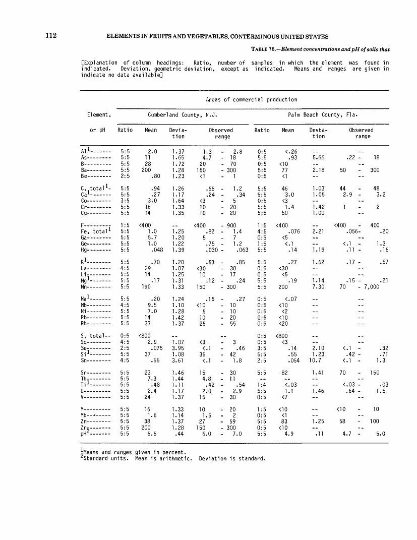
112 ELEMENTS IN FRUITS AND VEGETABLES, CONTERMINOUS UNITED STATES
TABLE 76.—Element concentrations and pH of soils that
[Explanation of column headings: Ratio, number of samples in which the element was found in indicated. Deviation, geometric deviation, except as indicated. Means and ranges are given in indicate no data available]
Areas of commercial production
Element,
or pH
All- ___.flc_____ __ _
D =
Be—- ———
C.total 1 - ral-Co — — —r r_ _ _____Cu— ———
F— ....Fe, total 1 Ga— — —Ge— ———Hg—— - —
IflLa--- ———1 i____.___
1 Mg 1 — — —Mn —————
M-,l_Nb — - ——NI —————Pb ——— --Rb — —— - —
S, total — Sc- __ ---SP __ _ -
1 Si 1 - _ ---Sn— —— --
Sr--------Th-- —— ...Til-——U ——————V _________
Y ——————WL
Zn — — —Zr —————PH2~~-
Cumberland County, N.J.
Ratio
5:5 5:5 5:5 5:5 2:5
5:5 5:5 3:5 5:5 5:5
1:5 5:5 5:5 5:5 5:5
5:5 4:5 5:5 5:5 5:5
5:5 4:5 5:5 5:5 5:5
0:5 4:5 2:5 5:5 4:5
5:5 5:5 5:5 5:5 5:5
5:5 5:5 5:5 5:5 5:5
Mean
2.0 11 28
200 .80
.94
.27 3.0
16 14
<400 1.0 5.7 1.0
.048
.70 29 14
.17 190
.20 9.5 7.0
14 37
<800 2.9
.075 37
.66
23 7.3
.48 2.4
24
16 1.6
38 200
6.6
Devia tion
1.37 1.65 1.72 1.28 1.23
1.26 1.17 1.64 1.33 1.35
1.25 1.20 1.22 1.39
1.20 1.07 1.25 1.31 1.33
1.24 1.10 1.28 1.42 1.37
1.07 3.95 1.08 3.61
1.46 1.44 1.11 1.17 1.37
1.33 1.14 1.37 1.28
.44
Observed range
1.3 4.7
20 150
<1
.66
.24 <3 10 10
<400 .82
5 .75 .030
.53 <30
10 .12
150
.15 <10
5 10 25
<3<.l
35 <.l
15 4.8
.42 2.0
15
10 1.5
27 150
6.0
- 2.8 - 18 - 70 - 300 - 1
- 1.2.34
5 - 20 - 20
- 900 - 1.4 - 7 - 1.2
.063
.85 - 30 - 17
.24 - 300
.27 - 10 - 10 - 20 - 55
- 3 .46
- 42 - 1.8
- 30 - 11
.54 - 2.9 - 30
- 20 - 2 - 59 - 300 - 7.0
Ratio
0:5 5:5 0:5 5:5 0:5
5:5 5:5 0:5 5:5 5:5
1:5 4:5 0:5 1:5 5:5
5:5 0:5 0:5 5:5 5:5
0:5 0:5 0:5 0:5 0:5
0:5 0:5 3:5 5:5 2:5
5:5
1:4 5:5 0:5
1:5 0:5 5:5 0:5 5:5
Palm Beach County, Fla.
Mean
<.26 .93
<10 77 <1
46 3.0
<3 1.4
50
<400 .076
<5 <.l
.14
.27 <30
<5 .19
200
<.07 <10
<2 <10 <20
<800 <3
.14
.55
.054
82
<.03 1.1
<7
<10 <1 83
<10 4.9
Devta- tion
5.66
2.18
1.03 1.05
1.42 1.00
2.21
1.19
1.62
1.14 7.30
2.10 1.23
10.7
1.41
1.46
1.25
.11
Observed range
.22 - 18
50 - 300
44 - 48 2.9 - 3.2
1 - 2
<400 - 400 .056- .20
<.l - 1.3 .11 - .16
.17 - .57
.15 - .21 70 - 7,000
<.l - .32 .42 - .71
<.l - 1.3
70 - 150
<.03 - .03 .64 - 1.5
<10 - 10
58 - 100
4.7 - 5.0
^Means and ranges given in percent.^Standard units. Mean is arithmetic. Deviation is standard.
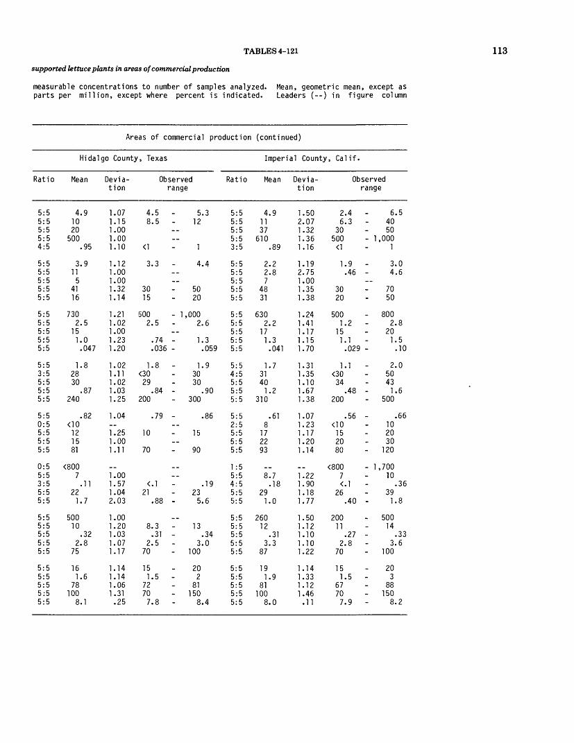
TABLES 4-121
supported lettuce plants in areas of commercial production
measurable concentrations to number of samples analyzed. Mean, geometric mean, except as parts per million, except where percent is indicated. Leaders (--) in figure column
113
Areas of commercial production (continued)
Hidalgo County, Texas
Ratio
5:55:55:55:54:5
5:55:55:55:55:5
5:55:55:55:55:5
5:53:55:55:55:5
5:50:55:55:55:5
0:55:53:55:55:5
5:55:55:55:55:5
5:55:55:55:55:5
Mean
4.91020
500.95
3.911
54116
7302.5
151.0.047
1.82830
.87240
.82<10
121581
<8007
.1122
1.7
50010
.322.8
75
161.6
78100
8.1
Devia tion
1.071.151.001.001.10
1.121.001.001.321.14
1.211.021.001.231.20
1.021.111.021.031.25
1.04—1.251.001.11
__1.001.571.042.03
1.001.201.031.071.17
1.141.141.061.31.25
Observed range
4.58.5
<1
3.3
3015
6002.5
.74
.036
1.8<30
29.84
200
.79
10
70
<.l21
.88
8.3.31
2.570
151.5
72707.8
5.312
--__
1
4.4____
5020
- 1,0002.6
--1.3.059
1.93030
.90- 300
.86__
15--
90
__--
.1923
5.6
__13
.343.0
- 100
202
81- 150
8.4
Ratio
5:55:55:55:53:5
5:55:55:55:55:5
5:55:55:55:55:5
5:54:55:55:55:5
5:52:55:55:55:5
1:55:54:55:55:5
5:55:55:55:55:5
5:55:55:55:55:5
Imperial County, Calif.
Mean
4.91137
610.89
2.22.87
4831
6302.2
171.3
.041
1.73140
1.2310
.618
172293
__8.7
.1829
1.0
26012
.313.3
87
191.9
81100
8.0
Devia tion
1.502.071.321.361.16
1.192.751.001.351.38
1.241.411.171.151.70
1.311.351.101.671.38
1.071.231.171.201.14
__1.221.901.181.77
1.501.121.101.101.22
1.141.331.121.46
.11
Observed range
2.46.3
30500
<1
1.9.46
3020
5001.2
151.1
.029
1.1<30
34.48
200
.56<10
152080
<8007<.l
26.40
20011
.272.8
70
151.5
67707.9
6.54050
- 1,0001
3.04.6
-_7050
- 8002.8
201.5
.10
2.05043
1.6- 500
.66102030
- 120
- 1,70010
.3639
1.8
- 50014
.333.6
- 100
203
88- 150
8.2

114 ELEMENTS IN FRUITS AND VEGETABLES, CONTERMINOUS UNITED STATES
TABLE 77.—Element concentrations and pH of soils that
[Explanation of column headings: Ratio, number of samples in which the element was found in indicated. Deviation, geometric deviation, except as indicated. Means and ranges are given in indicate no data available]
Areas of commercial production
Element,
or pH
All————
D ̂
Be ________
C, total 1-
Co— — —
Cu ——— —
F— ....Fe, total 1 Ga— -----Ge ——— —Hg——— —
K 1La-- — —Li— — -Mg 1 _______Mn— —— —
Nb —— — —
Pb — - ——
S, total —Sc --------Se------- -i Si 1 - ____Sn —— - —
Sr--- _ - _Th-—— —Til— — -U — ___—V _-_-____.
Y ——————Wl_
7«
Zr-— ——P
Wayne County, N.Y.
Ratio
5:5 5:5 4:5 5:5 0:5
5:5 5:5 4:5 5:5 5:5
2:5 5:5 4:5 5:5 5:5
5:5 0:5 4:5 5:5 5:5
4:5 1:5 5:5 5:5 4:5
2:5 4:5 5:5 5:5 4:5
5:5 4:4 5:5 5:5 4:5
4:5 4:5 5:5 4:5 5:5
Mean
2.6 13 16
240
5.9 1.0 4.3
17 17
374 1.2 7.9 1.0 .070
.92 <30 14
.24 145
.49
6.1 14 33
670 3.4 .34
20 .49
110 4.7 .26
2.4 22
12 1.3
46 118
4.8
Devia tion
1.99 1.85 1.55 2.10
3.61 2.27 1.38 2.09 2.41
1.45 1.34 1.60 1.99 2.55
2.00
1.97 1.51 1.54
3.45
1.36 1.35 1.49
1.75 1.44 1.84 3.19 3.81
1.38 1.15 2.40 1.47 2.53
1.39 1.60 1.26 6.02 6.30
Observed range
.77 6.2
70
2.0 .61
<3 5 7
500 .67
<5 .31 .024
.27
17 .12
70
<.07
5 1
<20
<800 <3
.13 2.5 <.l
70 4.1 .055
1.6 <7
36 <200
4.9
4.0 24 20
500
40 4.3 5
30 50
- 600 1.5
10 1.7 .31
1.4
22.33
- 200
1.0 10 10 20 50
- 1,500 5 .58
36 2.4
150 5.3 .41
4.5 50
15 2
64 - 500
6.8
Ratio
5:5 5:5 5:5 5:5 5:5
5:5 5:5 5:5 5:5 5:5
5:5 5:5 5:5 5:5 5:5
5:5 5:5 5:5 5:5 5:5
5:5 5:5 5:5 5:5 5:5
1:5 4:5 4:5 5:5 4:5
5:5 5:5 5:5 5:5 5:5
5:5 5:5 5:5 5:5 5:5
Cumberland County, N.J.
Mean
3.8 34 61
450 1.5
1.2 .38
6.1 59
140
700 2.0
11 1.3 .20
1.4 110 21
.35 220
.45 13 13 20 67
5.5 .25
35 .78
87 13
.62 4.6
57
44 4.5
51 255
5.5
Devia tion
1.06 1.30 1.20 1.26 1.46
1.31 1.07 1.20 1.46 1.29
1.39 1.07 1.20 1.11 1.32
1.07 2.52 1.06 1.10 1.35
1.04 1.25 1.25 1.00 1.02
1.63 2.42 1.02 4.36
1.22 1.14 1.03 1.04 1.20
1.44 1.26 1.12 1.25 .58
Observed range
3.6 24 50
300 1
.88
.34 5
30 100
500 1.8
10 1.2 .15
1.3 50 20
.30 150
.43 10 10
60
<800 <3 <.l
34 .97
70 11
.61 4.4
50
30 3
45 200
4.8
4.1 46 70
500 2
1.7 .40
7 70
- 150
- 1,200 2.1
15 1.5 2.7
1.5 - 500
23 .39
300
.48 15 15
75
- 810 7 .75
36 3.4
- 100 15
.65 4.9
70
70 5
61 300
6.3
and ranges given in percent. Standard units. Mean is arithmetic. Deviation is standard.
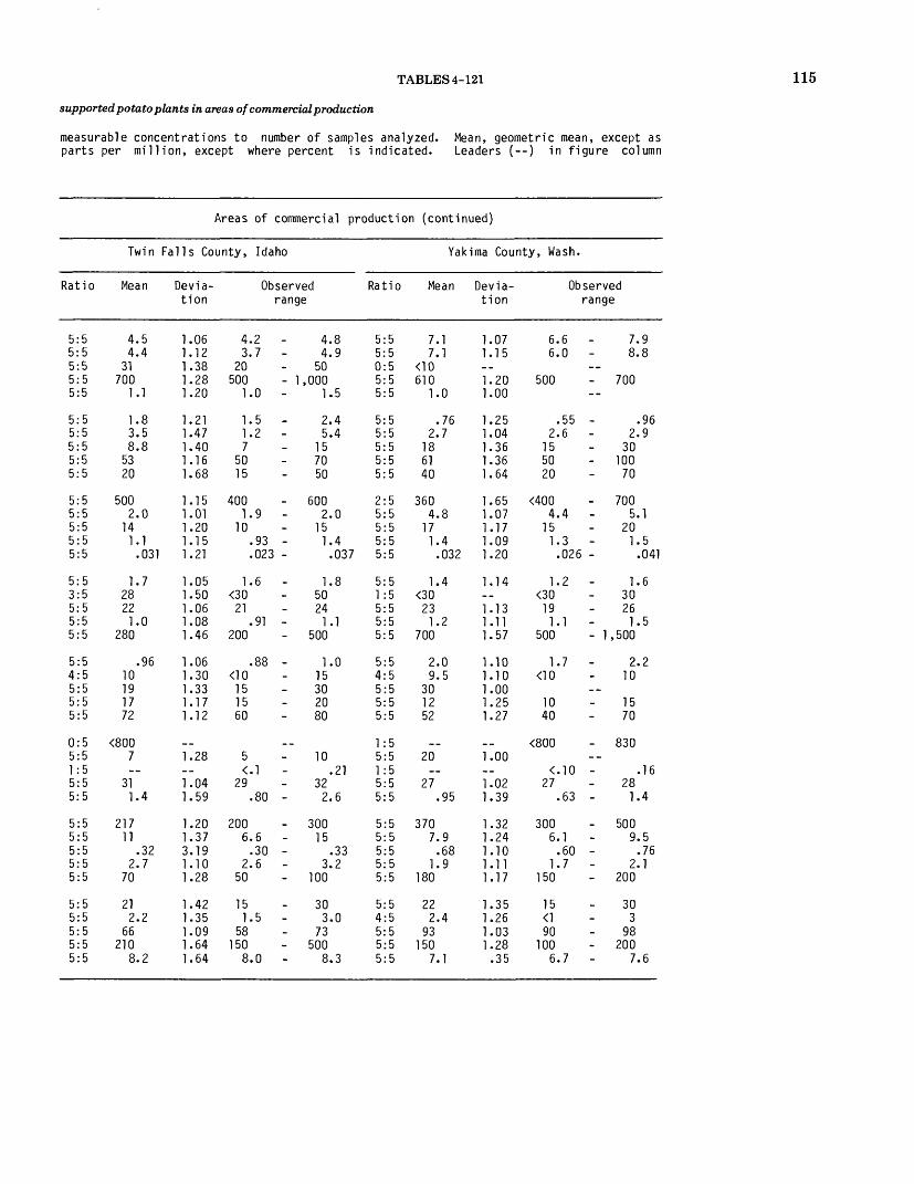
TABLES 4-121 115
supported potato plants in areas of commercial production
measurable concentrations to number of samples analyzed. Mean, geometric mean, except as parts per million, except where percent is indicated. Leaders (--) in figure column
Areas of commercial production (continued)
Twin Falls County, Idaho
Ratio
5:55:55:55:55:5
5:55:55:55:55:5
5:55:55:55:55:5
5:53:55:55:55:5
5:54:55:55:55:5
0:55:51:55:55:5
5:55:55:55:55:5
5:55:55:55:55:5
Mean
4.54.4
31700
1.1
1.83.58.8
5320
5002.0
141.1
.031
1.728221.0
280
.9610191772
<8007__
311.4
21711
.322.7
70
212.2
66210
8.2
Devia tion
1.061.121.381.281.20
1.211.471.401.161.68
1.151.011.201.151.21
1.051.501.061.081.46
1.061.301.331.171.12
__1.28__1.041.59
1.201.373.191.101.28
1.421.351.091.641.64
Observed range
4.23.7
20500
1.0
1.51.27
5015
4001.9
10.93.023
1.6<30
21.91
200
.88<10
151560
5<.l
29.80
2006.6
.302.6
50
151.5
58150
8.0
4.84.9
50- 1,000
1.5
2.45.4
157050
- 6002.0
151.4
.037
1.85024
1.1- 500
1.015302080
_ _
10.21
322.6
- 30015
.333.2
- 100
303.0
73- 500
8.3
Ratio
5:55:50:55:55:5
5:55:55:55:55:5
2:55:55:55:55:5
5:51:55:55:55:5
5:54:55:55:55:5
1:55:51:55:55:5
5:55:55:55:55:5
5:54:55:55:55:5
Yakima County, Wash.
Mean
7.17.1
<10610
1.0
.762.7
186140
3604.8
171.4
.032
1.4<30
231.2
700
2.09.5
301252
_ _
20__
27.95
3707.9
.681.9
180
222.4
93150
7.1
Devia tion
1.071.15__1.201.00
1.251.041.361.361.64
1.651.071.171.091.20
1.14__1.131.111.57
1.101.101.001.251.27
__1.00__1.021.39
1.321.241.101.111.17
1.351.261.031.28
.35
Observed range
6.66.0
500
.552.6
155020
<4004.4
151.3
.026
1.2<30
191.1
500
1.7<10
1040
<800
<.1027
.63
3006.1
.601.7
150
15<190
1006.7
7.98.8
__- 700--
.962.9
30- 100
70
- 7005.1
201.5
.041
1.630261.5
- 1,500
2.210
__1570
- 830--
.1628
1.4
- 5009.5
.762.1
- 200
303
98- 200
7.6
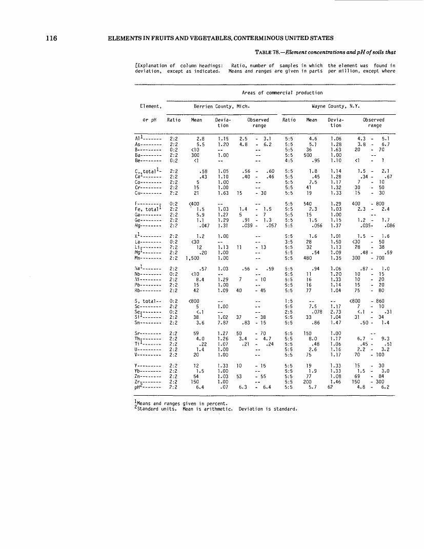
116 ELEMENTS IN FRUITS AND VEGETABLES, CONTERMINOUS UNITED STATES
TABLE 78.—Element concentrations and pH of soils that
[Explanation of column headings: deviation, except as indicated.
Ratio, number of samples in which Means and ranges are given in parts
the element was found in per million, except where
Areas of commercial production
Element,
or pH
All- . ..Ac_ __
D -,
Be —————
C^total 1 -r, 1
Co-- —— --Q r_ _ ___ _Cu- —— - ——
Fe, total 1 Ga——— ---Ge- — ----Hg— — -
K 1 —La —————Li-——Mg 1 ————Mn ———— --
Na 1 ————Nb —————Ni —————Pb —————DK
S, total — Sc ————Se —————Si 1- -
Sr — -----Th-~- —Ti 1 —— ---U ——————V ——————
Y ——————
Z n ——— --Zr—— - —nW-
Ratio
2:2 2:2 0:2 2:2 0:2
2:2 2:2 2:2 2:2 2:2
0:2 2:2 2:2 2:2 2:2
2:2 0:2 2:2 2:2 2:2
2:2 0:2 2:2 2:2 2:2
0:2 2:2 0:2 2:2 2:2
2:2 2:2 2:2 2:2 2:2
2:2 2:2 2:2 2:2 2:2
Berrien
Mean
2.8 5.5
<10 300
<1
.58
.43 5
15 21
<400 1.5 5.9 1.1 .047
1.2 <30
12 .20
1,500
.57 <10
8.4 15 42
<800 5 <•!
38 3.6
59 4.0
.22 1.4
20
12 1.5
54 150
6.4
County,
Devia tion
1.15 1.20
1.00
1.05 1.10 1.00 1.00 1.63
1.03 1.27 1.29 1.31
1.00
1.13 1.00 1.00
1.03
1.29 1.00 1.09
1.00
1.02 7.87
1.27 1.26 1.07 1.00 1.00
1.33 1.00 1.03 1.00 .07
Mich.
Observed range
2.5 - 3.1 4.8 - 6.2
.56 - .60
.40 - .46
15 - 30
1.4 - 1.5 5 - 7
.91 - 1.3
.039 - .057
11 - 13
.56 - .59
7 - 10
40 - 45
37 - 38 .83 - 15
50 - 70 3.4 - 4.7
.21 - .24
10 - 15
53 - 55
6.3 - 6.4
Ratio
5:5 5:5 5:5 5:5 4:5
5:5 5:5 5:5 5:5 5:5
5:5 5:5 5:5 5:5 5:5
5:5 3:5 5:5 5:5 5:5
5:5 5:5 5:5 5:5 5:5
1:5 5:5 2:5 5:5 5:5
5:5 5:5 5:5 5:5 5:5
5:5 5:5 5:5 5:5 5:5
Wayne
Mean
4.6 5.1
36 500
.95
1.8 .45
7.5 41 19
540 2.3
15 1.5
.056
1.6 28 32
.54 480
.94 11 16 16 77
7.5 .078
33 .86
150 8.0
.48 2.6
75
19 1.9
77 200
5.7
County,
Devia tion
1.06 1.28 1.63 1.00 1.10
1.14 1.28 1.17 1.32 1.33
1.29 1.03 1.00 1.15 1.37
1.01 1.50 1.13 1.09 1.35
1.06 1.20 1.33 1.14 1.04
1.17 2.73 1.04 1.47
1.00 1.17 1.06 1.16 1.17
1.33 1.33 1.08 1.46
62
N.Y.
Observed range
4.3 - 3.8 -
20
<1
1.5 - .34 -
7 30 15
400 2.3 -
1.2 - .035-
1.5 - <30
28 .48 -
300
.87 - 10 10 15 75
<800 7 <.l -
31 .50 -
6.7 - .45 -
2.2 - 70
15 1.5 -
69 150
4.8 -
5.1 6.7
70
1
2.1 .67
10 50 30
800 2.4
1.7 .086
1.6 50 38
.59 700
1.0 15 20 20 80
860 10
.31 34
1.4
9.3 .51
3.2 100
30 3.0
84 300
6.2
and ranges given in percent. Standard units. Mean is arithmetic. Deviation is standard.
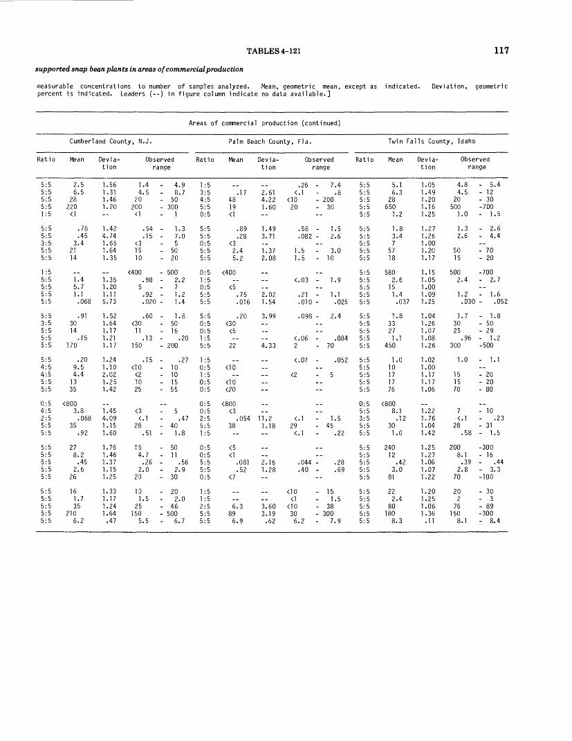
TABLES 4-121 117
supported snap bean plants in areas of commercial production
measurable concentrations to number of samples analyzed. Mean, geometric mean, except as indicated, percent is indicated. Leaders (--) in figure column indicate no data available.]
Deviation, geometric
Areas of commercial production (continued)
Cumberland County, N.J.
Ratio
5:55:55:55:51:5
5:55:53:55:55:5
1:55:55:55:55:5
5:53:55:55:55:5
5:54:54:55:55:5
0:54:52:55:55:5
5:55:55:55:55:5
5:55:55:55:55:5
Mean
2.56.5
28220<1
.78
.453.4
2114
__1.45.71.1.068
.913014
.15170
.209.54.41335
<8003.8.068
35.92
278.2.45
2.626
161.735
2106.2
Devia tion
1.561.311.461.20--
1.424.741.651.641.35
__1.351.201.115.73
1.521.641.171.211.17
1.241.102.021.251.42
__1.454.091.151.60
1.761.461.371.151.25
1.331.171.241.64.47
Observed range
1.44.5
20200<1
.54
.15<31510
<400.98
5.92.020
.60<3011
.13150
.15<10<21025
<3<.l
28.51
154.7.26
2.020
101.5
25150
5.5
4.9- 8.7- 50- 300- 1
- 1.37.0
- 5- 50- 20
- 5002.271.2
- 1.4
1.8- 50- 16
.20- 200
.27- 10- 10- 15- 55
__- 5
.47- 40
1.8
- 50- 11
.56- 2.9- 30
- 202.0
- 46- 500- 6.7
Ratio
1:53:54:55:50:5
5:55:50:55:55:5
0:51:50:55:55:5
5:50:50:51:55:5
1:50:51:50:50:5
0:50:52:55:51:5
0:50:55:55:50:5
1:51:52:55:55:5
Palm Beach County, Fla.
Mean
__.17
4819<1
.89
.28<32.45.2
<400._
<5.75.016
.20<30<5__
22
__<1 0
._<10<20
<800<3
.05438--
<5<]
.081
.52<7
..
._6.3
896.9
Devia tion
__2.614.221.60--
1.493.71__1.372.08
..____2.021.54
3.99______4.33
______—--
____11.21.18--
____2.161.28--
..__3.603.19.62
Observed range
.26 - 7.4<.l - .8
<10 - 20020 - 30
--
.58 - 1.5
.082 - 2.6__
1.5 - 3.01.5 - 10
__<.03 - 1.9
__.21 - 1.1.010 - .025
.098 - 2.4____
<.06 - .0842 - 70
<.07 - .052__
<2 - 5__--
____
<.l - 1.529 - 45<.l - .22
____
.044 - .28
.40 - .69--
<10 - 15<1 - 1.5
<10 - 3830 - 3006.2 - 7.9
Ratio
5:55:55:55:55:5
5:55:55:55:55:5
5:55:55:55:55:5
5:55:55:55:55:5
5:55:55:55:55:5
0:55:53:55:55:5
5:55:55:55:55:5
5:55:55:55:55:5
Twin Falls County, Idaho
Mean
5.16.3
28650
1.2
1.83.47
5718
5802.6
151.4.037
1.833271.1
450
1.010171776
<8008.1.12
301.0
24012
.423.0
81
222.4
80180
8.3
Devia tion
1.051.491.201.161.25
1.271.261.001.201.17
1.151.051.001.091.25
1.041.261.071.081.26
1.021.001.171.171.06
__1.221.761.041.42
1.251.271.061.071.22
1.201.251.061.36.11
Observed range
4.84.5
20500
1.0
1.32.6
5015
5002.4
1.2.030
1.73025
.96300
1.0
151570
7<.l
28.58
2008.1.39
2.870
202
76150
8.1
- 5.4- 12- 30-700- 1.5
- 2.6- 4.4—- 70- 20
-700- 2.7__- 1.6- .052
- 1.8- 50- 29- 1.2-500
- 1.1__- 20- 20- 80
__- 10- .23- 31- 1.5
-300- 16- .44- 3.3-100
- 30- 3- 89-300- 8.4
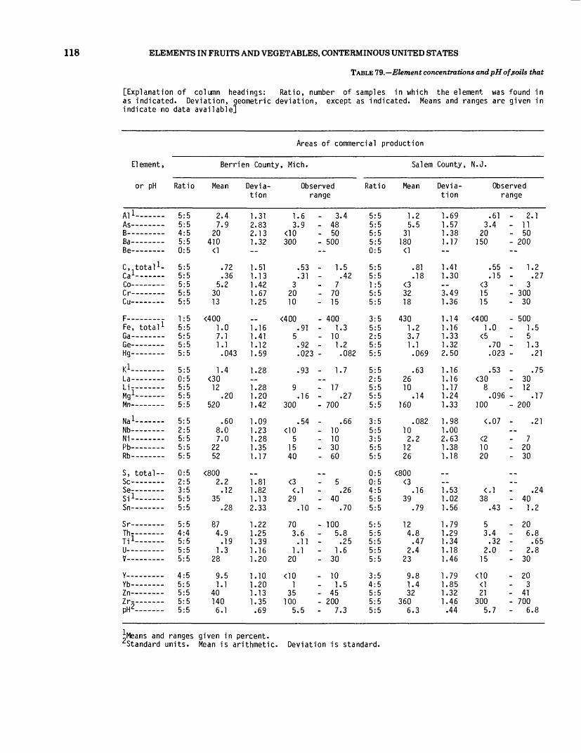
118 ELEMENTS IN FRUITS AND VEGETABLES, CONTERMINOUS UNITED STATES
TABLE 79.—Element concentrations and pH of foils that
[Explanation of column headings: Ratio, number of samples in which the element was found in as indicated. Deviation, geometric deviation, except as indicated. Means and ranges are given in indicate no data available]
Areas of commercial production
El ement ,
or pH
All-——AC __ ___ __ _
K =
D «
C.-total 1 -r a l__ _ _ _Co ——————Cr------ _Cu ——————
Fe, total 1 Ga —————Ge— — -Hg— — ~
KlLa — - ——li __ _ _
iMgl ——————Mm.
|\l=l__ __ _ __
Nb —————Ni —————Pb —— - ——nu.
S, total-- Sc~— —SP-- ___ -
i Si 1 -- __ _Sn —————
s r _ _ _ _ __Th- —— — -Til- ————U ——————V ——————
Y ——————vu.
Zn —————Zr —————nu2pH —————
Berrien County, Mich.
Ratio
5:5 5:5 4:5 5:5 0:5
5:5 5:5 5:5 5:5 5:5
1:5 5:5 5:5 5:5 5:5
5:5 0:5 5:5 5:5 5:5
5:5 2:5 5:5 5:5 5:5
0:5 2:5 3:5 5:5 5:5
5:5 4:4 5:5 5:5 5:5
4:5 5:5 5:5 5:5 5:5
Mean
2.4 7.9
20 410 <1
.72
.36 5.2
30 13
<400 1.0 7.1 1.1 .043
1.4 <30 12
.20 520
.60 8.0 7.0
22 52
<800 2.2 .12
35 .28
87 4.9 .19
1.3 28
9.5 1.1
40 140 6.1
Devia tion
1.31 2.83 2.13 1.32
1.51 1.13 1.42 1.67 1.25
1.16 1.41 1.12 1.59
1.28
1.28 1.20 1.42
1.09 1.23 1.28 1.35 1.17
1.81 1.82 1.13 2.33
1.22 1.25 1.39 1.16 1.20
1.10 1.20 1.13 1.35 .69
Observed range
1.6 3.9
<10 300
.53
.31 3 20 10
<400 .91
5 .92 .023
.93
9 .16
300
.54 <10
5 15 40
<3 <.l
29 .10
70 3.6 .11
1.1 20
<10 1
35 100
5.5
- 3.4 - 48 - 50 - 500
- 1.5 .42
7 - 70 - 15
- 400 - 1.3 - 10 - 1.2
.082
- 1.7
- 17 .27
- 700
.66 - 10 - 10 - 30 - 60
- 5 .26
- 40 .70
- 100 - 5.8
.25 - 1.6 - 30
- 10 - 1.5 - 45 - 200 - 7.3
Ratio
5:5 5:5 5:5 5:5 0:5
5:5 5:5 1:5 5:5 5:5
3:5 5:5 2:5 5:5 5:5
5:5 2:5 5:5 5:5 5:5
3:5 5:5 3:5 5:5 5:5
0:5 0:5 4:5 5:5 5:5
5:5 5:5 5:5 5:5 5:5
3:5 4:5 5:5 5:5 5:5
Salem
Mean
1.2 5.5
31 180 <1
.81
.18 <3 32 18
430 1.2 3.7 1.1 .069
.63 26 10
.14 160
.082 10 2.2
12 26
<800 <3
.16 39
.79
12 4.8 .47
2.4 23
9.8 1.4 32
360 6.3
County, N.J.
Devia tion
1.69 1.57 1.38 1.17
1.41 1.30
3.49 1.36
1.14 1.16 1.33 1.32 2.50
1.16 1.16 1.17 1.24 1.33
1.98 1.00 2.63 1.38 1.18
1.53 1.02 1.56
1.79 1.29 1.34 1.18 1.46
1.79 1.85 1.32 1.46 .44
Observed range
.61 3.4
20 150
.55
.15 <3 15 15
<400 1.0
<5 .70 .023
.53 <30
8 .096
100
<.07
<210 20
<.l38
.43
5 3.4 .32
2.0 15
<10 <1 21
300 5.7
- 2.1 - 11 - 50 - 200
- 1.2 .27
- 3 - 300 - 30
- 500 - 1.5 - 5 - 1.3
.21
.75 - 30 - 12
.17 - 200
.21
- 7 - 20 - 30
.24 - 40 - 1.2
- 20 - 6.8
.65 - 2.8 - 30
- 20 - 3 - 41 - 700 - 6.8
^Means and ranges given in percent.^Standard units. Mean is arithmetic. Deviation is standard.
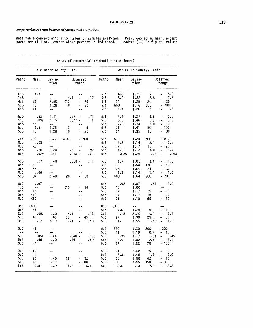
TABLES 4-121
supported sweet corn in areas of commercial production
measurable concentrations to number of samples analyzed. Mean, geometric mean, except parts per million, except where percent is indicated. Leaders (—) in figure column
119
Areas of commercial production (continued)
Palm Beach County, Fla.
Ratio
0:51:54:55:50:5
5:55:50:55:55:5
2:50:50:55:55:5
5:50:50:50:55:5
0:51:50:50:50:5
0:50:52.55:53:5
0:5--
5:55:50:5
0:50:55:55:55:5
Mean
<.3—
3415<1
.52
.092<34.5
15
390<.03
<5.76.029
.077<30 '<5<.06
34
<.07—
<2<10<20
<800<3
.09241
.17
<5—.054.56
<7
<10<120785.8
Devia tion
--2.581.28--
1.411.16—1.261.28
1.27—__1.201.41
1.40--____1.48
______----
__--1.301.053.19
_ _—1.241.20--
__--1.451.99.39
Observed Ratio range
5:5<.l - .12 5:5
<10 - 70 5:510 - 20 5:5
5:5
.32 - .71 5:5
.077 - .11 5:55:5
3-5 5:510 - 20 5:5
<400 - 500 5:55:55:5
.59 - .92 5:5
.018 - .040 5:5
.050 - .11 5:53:55:55:5
20 - 50 5:5
5:5<10 - 10 5:5
5:55:55:5
0:55:5
<.l - .13 3:538 - 43 5:5<.l - .53 5:5
5:55:5
.040 - .066 5:5
.44 - .69 5:55:5
5:55:5
12 - 32 5:530 - 200 5:55.5 - 6.4 5:5
Twin Falls County, Idaho
Mean
4.65.0
24650
1.1
2.45.37.5
7124
6302.3
171.2.035
1.730261.3
400
.9210171771
<8007.0.13
271.1
22011
.352.9
87
212.3
68230
8.0
Devia tion
1.151.381.251.161.20
1.271.461.341.411.38
1.241.141.171.121.25
1.051.641.091.141.64
1.071.001.171.171.10
_ _
1.282.201.081.55
1.201.191.171.081.22
1.421.461.081.46.13
Observed range
4.13.5
20500
1
1.62.95.0
5015
5002.1
151.0.024
1.6<30241.1
200
.87
151565
5<.l
25.69
2008.4.31
2.670
151.5
62150
7.9
- 5.8- 7.3- 30- 700- 1.5
- 3.0- 7.9- 10- 100- 30
- 800- 2.9- 20- 1.4
.043
- 1.8- 50- 30- 1.6- 700
- 1.0__- 20- 20- 80
__- 10- 3.1- 30- 1.9
-300- 13
.45- 3.1- 100
- 30- 3.0- 75- 300- 8.2
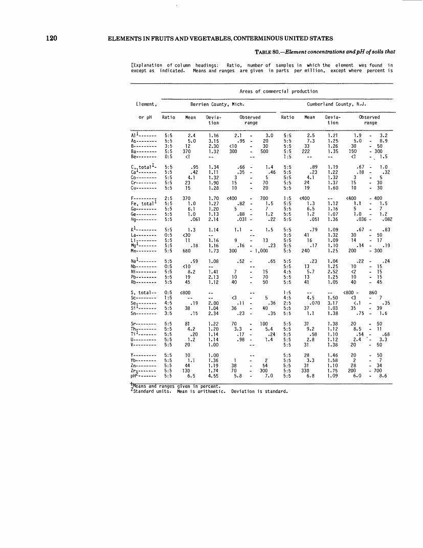
120 ELEMENTS IN FRUITS AND VEGETABLES, CONTERMINOUS UNITED STATES
TABLE SO.—Element concentrations and pH of soils that
[Explanation of column headings: Ratio, number of samples in which the element was found in except as indicated. Means and ranges are given in parts per million, except where percent is
Areas of commercial production
Element,
or pH
Al 1AO
n _
Be —————
C.-total 1 - r,lCo-- —— ——Qr_ _ _____Cu ———————
Fe, total 1 Ga — - ——Ge— — -Hg— — -
K1-La —————liii:~--:Mn —————
M-,1
Nb —————Ni— — -.Pb —————Rb —————
S, total — SC —————Cp_ ___ ____ie_ —— ____$jl _______S n —————
Th--— —Ti 1— — -U —————V —————
Y ——————
Zn —————Zr —pH2— — --u, ————— —
Berrien County, Mich.
Ratio
5:5 5:5 3:5 5:5 0:5
5:5 5:5 5:5 5:5 5:5
2:5 5:5 5:5 5:5 5:5
5:5 0:5 5:5 5:5 5:5
5:5 0:5 5:5 5:5 5:5
0:5 1:5 4:5 5:5 3:5
5:5 5:5 5:5 5:5 5:5
5:5 5:5 5:5 5:5 5:5
Mean
2.4 5.0
12 370 <1
.95
.42 4.1
23 15
370 1.0 6.1 1.0 .061
1.3 <30 11
.18 680
.59 <10
8.2 19 45
<800
.19 38
.15
81 4.2 .20
1.2 20
10 1.1
44 130
6.5
Devia tion
1.16 3.15 2.30 1.32
1.34 1.11 1.32 1.90 1.28
1.70 1.27 1.20 1.13 2.14
1.14
1.16 1.16 1.73
1.08
1.41 2.13 1.12
2.00 1.04 2.34
1.22 1.20 1.14 1.14 1.00
1.00 1.36 1.19 1.74 4.55
Observed range
2.1 .95
<10 300
.66
.35 3
15 10
<400 .B2
5 .88 .031
1.1
9 .16
300
.52
7 10 40
<3.11
36 .23
70 3.3 .17 .98
1 38 70 5.8
3.0 20 30
- 500
1.4 .46
5 70 20
- 700 1.5 7 1.2 .22
1.5
13 .23
- 1,000
.65
15 70 50
5 .36
40 .35
- 100 5.4 .24
1.4
2 54
- 300 7.0
Ratio
5:5 5:5 5:5 5:5 1:5
5:5 5:5 5:5 5:5 5:5
1:5 5:5 5:5 5:5 5:5
5:5 5:5 5:5 5:5 5:5
5:5 5:5 4:5 5:5 5:5
1:54:5 2:5 5:5 5:5
5:5 5:5 5:5 5:5 5:5
5:5 5:5 5:5 5:5 5:5
Cumberland County, N.J.
Mean
2.5 7.3
33 222
.89
.23 4.1
24 19
<400 1.3 6.5 1.2 .051
.79 41 16 .17
240
.23 13 5.7
13 41
4.5 .070
37 1.1
31 9.2 .58
2.8 31
28 3.3
31 330
6.8
Devia tion
1.21 1.25 1.26 1.35
1.19 1.22 1.32 1.37 1.60
1.12 1.16 1.07 1.36
1.09 1.32 1.09 1.10 1.25
1.04 1.25 2.52 1.25 1.05
1.50 3.17 1.03 1.38
1.38 1.12 1.10 1.12 1.38
1.46 1.58 1.10 1.75 1.09
Observed range
1.9 5.0
30 150 <1
.67
.18 3
15 10
<400 1.1 5 1.0 .036
.67 30 14
.14 200
.22 10 <2 10 40
<800 - <3 <.l
35 .75
20 8.5 .54 2.4 '
20
20 2
28 200
6.0
- 3.2 - 8.9 - 50 - 300- v 1.5
- 1.0 .32
- 5 - 30 - 30
- 400 - 1.5 - 7 - 1.2
.082
.83 - 50 - 17
.19 - 300
.24 - 15 - 15 - 15 - 45
860 - 7
.35 - 39 - 1.6
- 50 - 11
.68 - 3.3 - 50
- 50 - 7 - 34 - 700 - 8.6
^Means and ranges given in percent. ^Standard units. Mean is arithmetic. Deviation is standard.

TABLES 4-121 121
supported tomato plants in areas of commercial production
measurable concentrations to number of samples analyzed. Mean, geometric mean, except as indicated, indicated. Leaders (--) in figure column indicate no data available.]
Deviation, geometric deviation,
Areas of commercial production (continued)
Palm Beach County, Fla. Yakima County, Wash. San Joaquin County, Calif.
Ratio
0:52:50:55:50:5
5:55:51:55:55:5
0:50:50:55:55:5
5:50:50:51:55:5
0:51:50:50:50:5
0:50:50:55:51:5
0:5__
5:55:50:5
0:50:55:55:55:5
Mean
<.26.070
<1017<1
.58
.29»2.7
45
<400<.03
<5.81.020
.099<30
<5<.06
57
<.07 '—
<2<10<20
<800<3<.l
39—
<5__
.053
.58<7
<10<121
1408.2
Devia- Observed tion range
14.1 <.l - 1.3—1.17 15 - 20--
1.15 .53 - .741.29 .20 - .40
<3 - 52.85 1 - 151.60 20 - 70
__——1.23 .59 - 1.01.51 .010 - .03
1.17 .076 - .12—__
<.06 - .061.20 50 - 70
__<10 - 15
____—
___—1.10 35 - 44
<.l - .85
__—1.21 .039 - .0671.14 .47 - .65--
____1.05 20 — 231.35 100 - 200
.50 7.4 - 8.7
Ratio
5:55:50:55:54:5
5:55:55:55:55:5
3:55:55:55:55:5
5:50:55:55:55:5
5:52:55:55:55:5
1:55:51:55:55:5
5:55:55:55:55:5
5:53:35:55:55:5
Mean
7.45.5
<10620
.95
.572.9
178837
<4004.9
201.4
.046
1.3<30
221.2
700
2.08.0
301046
__20
._271.0
4106.2
.641.8
160
182
96120
6.6
Devia tion
1.051.38__1.631.10
1.101.021.171.401.32
__1.041.001.151.32
1.03__1.031.021.41
1.041.231.001.001.10
__1.00__1.041.51
1.321.111.041.211.14
1.361.001.081.25
.26
Observed range
6.93.6
500<1
.512.8
157030
<4004.8
1.2.03
1.3
211.2
500
1.9<10
40
<800
<.l26
.52
3005.2.62
1.5150
15
86100
6.3
7.78.4
__- 1,500
1
.642.9
20- 150
50
- 4005.2
__1.7
.67
1.4__
231.3
- 1,000
2.110
____
50
- 940__
.1828
1.5
- 5007.0.68
2.4- 200
30__— 100- 150
6.9
Ratio
5:55:50:55:55:5
5:55:55:55:55:5
1:55:55:55:55:5
5:50:55:55:55:5
5:53:55:55:55:5
0:55:51:55:54:5
5:55:55:55:55:5
5:55:55:55:55:5
Mean
6.93.3
<10870
1.0
.402.76.1
208.1
__2.4
181.0
.026
2.1<30
13.58
280
2.78.9
101675
<8006.5__
29.53
81015
.333.0
93
111.2
48100
8.5
Devia tion
1.021.25__1.221.00
1.231.021.21.281.22
__1.081.171.141.72
1.02-_1.081.041.20
1.021.161.311.141.07
__1.16—1.053.13
1.221.441.031.081.17
1.201.251.141.46
.22
Observed range
6.82.7
700
.292.75
157
<4002.3
15.87.010
2.0
12.56
200
2.6<10
7.01570
5<.l
27.75
70010
.322.7
70
101.0
40708.2
7.14.8
__- 1,000--
.482.87
3010
- 5002.7
201.2
.039
2.1—
15.62
- 300
2.810152080
__7
.1130
1.4
- 1,00024
.343.3
- 100
151.5
55- 150
8.7

122 ELEMENTS IN FRUITS AND VEGETABLES, CONTERMINOUS UNITED STATES
TABLE 81.—Summary statistics of element concentrations andpH of soils that supported American grape vines inthree areas of commercial production
Ltxplanation of column headings: Ratio, number of samples in which the element was found in measurable concentrations to number of samples analyzed. Mean, geometric mean, except as indicated. Deviation, geometric deviation, except as indicated. Means and ranges are given in parts per million, except as indicated]
Element,or pH
All ——-As--------
D -.
Be— — -
C.total 1 -Ca 1 — — -Co— -----Cr—— ——
Fe, total *
Ge—— — -Hg——— —
l/lLa —————Li —————Mg 1 ——————Mn ———— ——
Ratio
15:1515:1511:1515:154:15
15:1515:1515:1515-1515:15
6:1515:1515:1515:1515:15
15:155-1 5
15:1515:15IR-IR
Mean Devia-
4.15.9
17470
.72
1.81.07.5
2934
3102.2
121.3
.042
1.52117
.4947D
tion
1.40I /TO
2.121 OC
1.29
1.622.481.731.672.21
") Of}
1.781.551.171 CO
1.151.691.292.21i .fid
Observedrange
1.9 -2.9 -
<10300
<1
.56 -
.35 -3
157
<400.97 -
5.97 -
<.01 -
1.2 -30
9.16 -
?nn
6.31550
7001
3.34.2
1570
150
1,400 4.8
201.6
.092
1.9
27 1.5
i nnn
Element,or pH
Na 1 — -Nb ———Ni ————Pb— —Rb — —
S, totalSc ———
iSn ———
Sr ————Th— —Ti 1 ———U ————V ————
Y ————
Zn —— -- Zr--—nH£ ____
Ratio
15:1511:15
15:15
4:1514:15
8 . 1 C
15:1515:15
15:1514:1415:15
15:15
15:1515:15i (;•!(;
Mean
1.09.4
122054
6806.8
.1132
7Q
1606.6
.402.0
59
161 Q
76190
fi a
Deviation
1.541.121.591.661.21
1.312.241.90
1.73
1 C.Q
1.451 571.292 no
1.471.521.751.77
07
Observedrange
.57 -<10
71040
<800<3<.l -
O£
9D
703.8 -
.16 -
.92 -20
<10<14270
a. R
1.810305075
1,10020
OQ
2.7
30012
7Q
2 c
150
303
410700
R n
^Means and ranges given in percent.^Standard units. Mean is arithmetic; deviation is standard.
TABLE 82.—Summary statistics of element concentrations and pH of soils that supported apple trees in five areasof commercial production
[Explanation of column headings: Ratio, number of samples in which the element was found in measurable concentrations to number of samples analyzed. Mean, geometric mean, except as indicated. Deviation, geometric deviation, except as indicated. Means and ranges are given in parts per million, except as indicated]
Element,or pH
All-——flc_ __ _ __ __
D^
Be—- — -
C.-total 1 -Ca 1 —— —Co —————
F— — —Fe, total 1Ga-- — --Ge ——— ---Hg— ———
I/ILa —————Li .....Mg 1 ————Mn —————
Ratio
25:2525:2519:2525:259'25
25:2525:2520:25
o c . oc
13-2525:25?1 -PS24:2525:25
o c . o c.
25:2525:2525:25
Mean
3.32720
3507Q
1.7.82
53324
4001.849.8
.92
.09
1.34017
.42290
Deviation
1.982.502 Cf-
1.651.24
1.742.982 151.711 RQ
1.591.682 f\f-
1.792.79
1.511 QT
1 CO
2.562.20
Observedrange
.67 -5.6 -
<10150
<1
.34 -
.13 -<31510
<400.83 -
<5<.l -
.01 -
.57 -<30
7.11 -
100
8.0135
701,000
1
3.53.0
207070
9004.7
201 CQ
.68
2.010037
1.31,500
Element,or pH
Na 1 ———Nb— —Ni ———Pb —— --Rh ---
S, totalSc ———
i Si 1 — --Sn ————
Sr ————Th— - -Ti 1 — -U ————V ————
Y ————Yb ————Zn ————Zr-———pH 2— -
Ratio
24:2617:2522:25o c . o c
25-25
8:2518:258:24
25-2523-25
25-2522:2225-2525:2525:25
24:2523:2425'2525:2525:25
Mean
.579.28 1
12049
6604.6
.060•33
.7
1046.8
1Q
2.249
131.5
1906.4
Deviation
3.001.142.702 Q£
1.61
1.492.493.241.16•5 04
3.481.511 531.462.33
1 ?41 351.561.861.03
Observedrange
<.07<10
<22020
<800<3<.l
26<.l
103.2
.171.0
10
<10<142
1004.6
2.21030
- 1,000- 1,000
- 1,60020
.6141
.69
50012
.724.0
- 200
202
- 200- 700
7.9
^Means and ranges given in percent.^Standard units. Mean is arithmetic; deviation is standard.
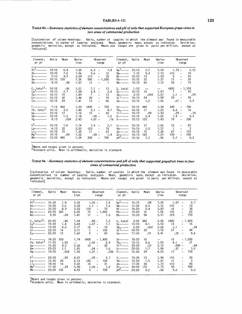
TABLES 4-121
TABLE 83.—Summary statistics of element concentrations andpH of soils that supported European grape vines intwo areas of commercial production
[Explanation of column headings: Ratio, number of samples in which the element was found in measurable concentrations to number of samples analyzed. Mean, geometric mean, except as indicated. Deviation, geometric deviation, except as indicated. Means and ranges are given in parts per million, except as indicated]
123
Element,or pH
Al 1 ——— -Ac_ __ ___
n-
Be —————
C^total 1 -Ca 1 --- — -Co ——— --
Cu--- — --
Fe, total 1Ga ————Ge— — —Un
K 1La — — —Li- _______
Mn — — _ —
Ratio
10:1010:103:10
10:109:10
10:1010:1010:1010:1010:10
7:1010:1010:1010:109:10
10:104:10
10:1010:1010:10
Mean
6.87.04.5
730QQ
.962.7
103224
4603.5
171.3
.024
1 Q
2216
.89440
Deviation
1.051.56
3 r-e\
1.361.07
1.211.081.491.461.41
1.291.401.161 1 Q
2.43
1.142.021 "3D
1.521.34
Observedrange
6.3 -3.6 -
500
7.1 -2.4 -7
2015
<4002.1 -
.94 -
1.5 -<30
11.58 -
300
7.41230
1,0001
133.0
7050
7004.7
201.5
.16
2.17023
1.4700
Element,or pH
Na 1 ———Nb — —
Pb-- —Rb -— —
S, totalSc — — —
iSn — —
Sr — —Th— —Ti 1 -- —U _______V ————
Y __— — _Yb — —Zn — —Zr- — —PHZ-—
Ratio
10:107:10
10:1010:1010:10
1:1010:103:10
10:1010:10
10:1010:1010:1010:1010:10
10:1010:1010:1010:1010:10
Mean
2.19.3
132066
12.060
291.2
44011
.492.4
120
172.0
72160
7.2
Deviation
1.141.13
1.371.12
1.472.571.041.55
1.2059
.25
.43f)C
.37"3D
.25
.96
Observedrange
1.78 -^i n
15
<8007, •»
9Q
.67 -
3008.6 -
.29 -1.9 -
70
101
47100
5.7 -
2.52102030
1,10020
.2930
2 5
70016
7Q
3.3200
203
120200
8.3
*Means and ranges given in percent.^Standard units. Mean is arithmetic; deviation is standard.
TABLE 84. -Summary statistics of element concentrations andpH of soils that supported grapefruit trees in fourareas of commercial production
[Explanation of column headings: Ratio, number of samples in which the element was found in measurable concentrations to number of samples analyzed. Mean, geometric mean, except as indicated. Deviation, geometric deviation, except as indicated. Means and ranges are given in parts per million, except as indicated]
Element,or pH
Al 1 — — -
Be—— ——
C.total 1 -Ca 1 — — -Co— — —
Cu- —— ---
Fe, total 1Ga-- —— -Ge— — —Hg—— — -
K lLa — — —Li_ _______
Ratio
16:2019:2010:2020:209:20
20:2019:2013:2020:2020:20
14:2017:2015:2020:2019:20
20:2010:20i Q -9n17:2020:20
Mean
1.92.28.9
320on
.861.4
1612
560<.039.31.1
.022
.99
16.34
150
Deviation
5.55o on
3.036.051.41
1.543.492.173.711.60
1.74
2 0/r
1.52
4.222.122.023.904.83
Observedrange
<.26 -* 1
<"in15
.48 -<.07 -
<315
<400<.03 -
.64 -
.05 -<30
<.06 -5
7.47.2
701,500
1 5
7.37.1
1010030
1,4002.9
301.6
.036
2.7100
311.2
700
Element,or pH
Na 1 ———Nb — —Nl— — —Pb — —Rb — —
S, totalSc — —Se— —Si 1 ———Sn — —
Sr — —Th ------Ti 1 — —U _______V _______
Y _______
Zn — —Zr — —pH2~—
Ratio
16:2012:2014:2015:2015:20
3:2013:20
6 . 9n
20:2017:20
i Q • 9n15:1520:2020:2016:20
15:2015:2017:2020:2020:20
Mean
.488.95 4
1254
3804.1
Dfi?
33.51
<59.6
.221.7
29
131.5
34170
8.2
Deviation
7.381.16
? 37
2.052.532 CQ
1 1 Q
1.552.121.894.20
1.941 Q7
1.731.73.98
Observedrange
<.07 -{ i n
<2
<20
<800<3
s -I
27
<54.1 -
.049 -
.37 -<7
ln,._505.0 -
2.7103020
120
1,50015
34449.6
1,00021
.441 9
150
303
5009.3
*Means and ranges given in percent.^Standard units. Mean is arithmetic; deviation is standard.
124 ELEMENTS IN FRUITS AND VEGETABLES, CONTERMINOUS UNITED STATES
TABLE 85.—Summary statistics of element concentrations and pH of soils that supported orange trees in fourareas of commercial production
[Explanation of column headings: Ratio, number of samples in which the element was found in measurable concentrations to number of samples analyzed. Mean, geometric mean, except as indicated. Deviation, geometric deviation, except as indicated. Means and ranges are given in parts per million, except as indicated]
Element,or pH
All——-Ac__ __ ___
D -.
Be — — —
C^total 1 -Ca 1 — - —Co — — —
Fe, total 1Ga—— — -Ge— - ——Hg— -—
K 1La— ———Li —————Mg 1 —————Mn —————
Ratio
14:2017:2010:2020:2013:20
20:2018:2013:2019:2020:20
13:2015:2015:2020:2020:20
20:207:20
i Q • on15:2020:20
Mean
<.261.49.3
330.91
.61
.68
1613
<.038 Q
1.0.024
on1613
.26140
Deviation
__4.662 c -j
5.921.22
1.594.822.114.40
2 c o
1.43
2.301 QG
1.58
4 QC
1 0?1.994.134.39
Observedrange
<.26 -<.l -
<1015<1
.32 -<.07 -
<3<1
7
<400<.03 -
<5
.01 -
.04 -<30
<5.06 -
1
7.45.0
501,500
1.5
2.63.7
10100300
9002.6
201.4
.059
2.715029
1.1700
Element,or pH
Na 1 ———Nb ———Ni ———Pb ————Rb ————
S, totalSc ———
i Si 1 ———Sn ——— -
Sr ———Th ———Ti ————U ————V ————
Y ————
Zn ———Zr— —pH 2———
Rat i o
15:2012:2015:2015:2015:20
2:2013:20
6 . on
20:2017:20
16:2016:1620:2020:2015:20
15:2016:2017:2020:2020:20
Mean
.498 Q
5.91249
8803.9
nco
35.39
8.9.20
1.625
121.3
<10190
7.8
Deviation
5.851.163 531.532 43
1.132.113.151.202.40
1.742.051 QO
4.17
1.591.53
1.571.31
Observedrange
<.07 -<10
<2<10<20
<800<3<.l -
27<.l -
<53
.06 -
.37 -<7
<10<1
<10100
5.0 -
2.7103020
100
96010
.3145
1.3
1,00019
.382.6
100
303
on
7009.3
^Means and ranges given in percent.^Standard units. Mean is arithmetic; deviation is standard.
TABLE 86.—Summary statistics of element concentrations andpHof soils that supported peach trees infourareasof commercial production
[Explanation of column headings: Ratio, number of samples in which the element was found in measurable concentrations to number of samples analyzed. Mean, geometric mean, except as indicated. Deviation, geometric deviation, except as indicated. Means and ranges are given in parts per million, except as indicated]
Element,or pH
All--—Ac- _ __ _
Ra
Be--— —
C^total 1 -Ca 1 —— —Co —— - —
C U - — — -
Fe, total 1Ga— ———Ge — — ——Hg———— -
K lLa —————Li- — . ...
Mn — ———
Ratio
20:2020:2014:2020:2011:20
20:2020:2020:2020:2020:20
16:2020:2020:2019:2020:20
20:206 . nri
20:2020:2020:20
Mean
5.37.5
17520
Q7
2.01.79.2
*3C
5103.0
161.1
1.61925
.90330
Deviation
1.254.232.721.331.27
1.391.841.731.992.11
1.561.471.201 QG
1 *3Q
1.161.701.301.671.86
Observedrange
3.5 -r\£
300
1.2 -.56 -
2015
<4001.7 -
10CO
n oc
1.3 -<30
17.33 -
150 -
6.9i no
70 700
1.5
3.13.1
20 200150
1,600 4.5
201.6
HOC
2.07040
1.31,000
Element,or pH
Na 1 — —Nb — — Ni ———Pb ———
S, totalSc — —
1 Si 1 - ——Sn — —
Sr ——— - Th— —Ti 1 -- —U ————V— - ...
Y.- ————wl
Zn — —Zr- ———pH2— -
Ratio
20:2014:2020:2020:2020:20
12:2020:207:20
20:2019:20
20:2020:2020:2020:2020:20
20:201 Q • 1 Q
20:2020:2020:20
Mean
1.09.3
203366
8709.9
.07229
7Q
2108.6
.462.5
100
161 Q
OQ
1506.4
Deviation
1.471.132.013.241 OO
1.961.67L. . J /
1.092.14
1.711.501.35i . ^ i 1.73
1 O C
1.321.581.03
Observedrange
.63 -j,-t n
7 1040
<8005> i
9C
1003.3 -.29 -
1.9 -30
101.5 -
CO
704.3 -
1.910
100300100
4,10020
351.7
50019
.664.0
200
303
140500
8.0
-Means and ranges given in percent.^Standard units. Mean is arithmetic; deviation is standard.
TABLES 4-121 125
TABLE 87.—Summary statistics of element concentrations andpH of soils that supported pear trees in five areasof commercial production
[Explanation of column headings: Ratio, number of samples in which the element was found in measurable concentrations to number of samples analyzed. Mean, geometric mean, except as indicated. Deviation, geometric deviation, except as indicated. Means and ranges are given in parts per million, except as indicated]
Element,or pH
All——-Ac _ __ _
R-,Q
C, total 1 -Ca 1 —— —Co- ———o_ __ ___
Fe, total 1GA-Ge ———— -Hg——— —
K 1 — — -La —————Li — — - -Mg 1 ————Mn —————
Ratio
25:25
f\ r\ , f\ t-
25-25
25:2525:2524-2525-2525-2 ci
18:2525:2525-25
25:25
25-257-2 (>
25-2525:2525:25
Mean
4.9102154 n
.92
2.11.38 0
4640
5102.5
141.2
.047
1.72424
.72380
Deviation
1.432.102 (\£-
1.432.751.751.92
1.501.671 451.241.74
1.141.201 341.981.85
Observedrange
2.2 -1.1 -
<10200
<1
.84 -
.29 -<315
7
<400.97 -
5.71 -.019-
1.2 -<30
10.16 -
150
7.92950
1,0003
3.86.5
20200300
1,2005.1
201.72.0
2.13034
1.41,000
Element,or pH
Na 1 ———Nb——— -Ni— —Pb ———Rh
S, totalSc ———
iSn ———
Th——Ti 1 — -U ————V ————
Y ————Yb ————Zn ————Zr ————pH— —
Ratio
25:25
3:2524:25
25-2524:25
23:2325'25
25:25
24:24
25:25,25:25
Mean
.968.9
1 Q
4269
5708.5
.09230
art
1909.1
312.4
78
171.7
1406.7
Deviation
1.471.162.192 351 O. C
1.341.942.971.151.77
1.911.391 OQ
1.291.91
1 0Q
1 "39
1.611.621.02
Observedrange
.30 -<10
51030
<800<3<.l -
24<.l -
705.2 -.14 -
20
101
31704.5 -
1.810
150200110
99020
/TO
371.5
50018
.423 C
200
303
210500
8.1
*Means and ranges given in percent.^Standard units. Mean is arithmetic; deviation is standard.
TABLE 88.—Summary statistics of element concentrations and pH of soils that supported plum trees infourareasof commercial production
[Explanation of column headings: Ratio, number of samples in which the element was found in measurable concentrations to number of samples analyzed. Mean, geometric mean, except as indicated. Deviation, geometric deviation, except as indicated. Means and ranges are given in parts per million, except as indicated]
Element,or pH
All-——Ac ___
D-.
Be—-- —
Cj.totall-Ca l— ——Co-- — ---Cr- _ _ ___C U —————
Fe, total 1Ga ——— —Ge — - ——Hg— -----
K lLa — - —
Mgl ————
Ratio
20:2020:2016:2020:2012:20
20:2020:2020:2020:2020:20
17:2020:2020:2020:2020:20
20:2011:2020:2020:2020:20
Mean
4.7
24490
.89
2.01.27.4
44f\C
con
2.4141.2
1.727
.66390
Deviation
1.402 /-r
1.16
1.592.351 CO
1 521 Q7
1.401.771.51
2.92
1.151.12
2.212.12
Observedrange
2.3 -
<10300
<1
.81 -
.32 -
1510
<400.84 -
.01 -
1.2 -<30
8 C\
.13 -150
7.49170
7001
6.13.5
20100150
9005.1
201.5
2 c
2.230
1.41,500
Element,or pH
Na 1 — -Nb ————Ni ————Pb ————Rb ————
S, totalSc— —
iSn ———
Th— —Ti 1 ———U- —— —V ————
Y ————yi
Zn ———Zr- ———PH2———
Ratio
20:2016:2020:2020:2020:20
6:2019:209:20
20:20i Q • or\
20:2020:2020:2020:2020:20
19:2019:1920:2020:2020:20
Mean
.96
155069
6707.6
.09130
on
i on8.3
.43
75
171 Q
100170
6.7
Deviation
1.551.10
1.29
1.421.792.911.133 /TO
1 O C
1.62.54.45
.47
.40
.571.56
.81
Observedrange
.49 -<10
510
800<3<.l -
f)C
<.l -
703.0 -
1 Q
1.1 -15
<101
OQ
1005.2 -
1.910
500110
1,40020
OQ
50017
7Q
200
303
310500
7.9
*Means and ranges given in percent.^Standard units. Mean is arithmetic; deviation is standard.

126 ELEMENTS IN FRUITS AND VEGETABLES, CONTERMINOUS UNITED STATES
TABLE 89.— Summary statistics of element concentrations and pH of soils that supported cabbage plants in twoareas of commercial production
[Explanation of column headings: Ratio, number of samples in which the element was found in measurable concentrations to number of samples analyzed. Mean, geometric mean, except as indicated. Deviation, geometric deviation, except as indicated. Means and ranges are given in parts per million, except as indicated]
Element,or pH
All- — —Ac----
n ..
Be—— — -
C.total 1 -Ca 1 — — -
Fe, total 1Ga— — --Ge — - ——H 9 ——— —
K 1La —————Li ——Mg 1 ——————Mn —————
Ratio
10:1010:1010:1010:10
7:10
10:1010:1010:1010:1010:10
10:1010:1010:1010:1010:10
10:105:10
10:1010:1010:10
Mean
5.16.7
30440
2.67.95.5
4421
6802.4
151.2
.031
1 Q
27321.0
260
Deviation
1.081.231.49
1.13
2.031.691 1 Q
1.341.50
1.251.131.101.191.24
1.061.141.111.541.23
Observedrange
4.4 -4.9 -
20300
<1
.48 -4.15
3015
5001.8 -
15QQ
.023 -
1.7 -<30
9D
.39 -200
5.88.9
50700
1
4.713
77050
1,000 2.7
201.5.042
2.03037 1.6
300
El ement ,or pH
Na 1 ———Nb ———Ni ——— . Pb ———Rb ———
S, totalSc ———
1 Si 1 ———Sn—— --
Th— —Ti 1 ———U ———— V ————
Y ————Vk
Zn ———Zr— —pH 2 ———
Ratio
10:106:10
10:1010:1010:10
1:1010:106:10
10:1010:10
10:1010:1010:1010:1010:10
10:1010:1010:1010:1010:10
Mean
.638.9
131584
7.5.13
24.92
oon
10.31
3.078
151.5
7Q
1108.1
Deviation
1.081.16
1 1 Q
1.07
1.252.001 1 Q
1.461.201.051.091.19
1.101.101.101.401.34
Observedrange
.56 -<10
71075
<8005<.l -
20CO
2008.2 -
o a2.5 -
70
151.5 -
60707.9 -
.6910202090
1,10010
301.2
70013
32
100
202
Bd
1508.3
^Means and ranges given in percent.^Standard units. Mean is arithmetic; deviation is standard.
TABLE 90.—Summary statistics of element concentrations and pH of soils that supported carrot plants in twoareas of commercial production
[Explanation of column headings: Ratio, number of samples in which the element was found in measurable concentrations to number of samples analyzed. Mean, geometric mean, except as indicated. Deviation, geometric deviation, except as indicated. Means and ranges are given in parts per million, except as indicated]
Element, or pH
Al 1 — — -
Pa
Be —— - —
C.-total 1 -
Co —————Cr —————Cu— — -.
Fe, total 1 Ga —————Ge —————Hg— — -
K 1La —————Li —————Mg 1 ——————Mn ————
Ratio
10:10 10:10 10:10 10:10 6:10
10:10 10:10 10:10 10:10 10:10
6:10 10:10 10:10 10:10 9:10
10:10 3:10
10:10 10:10 10:10
Mean Devia tion
4.8 6.9
38 530
.89
1.6 3.3 5.9
33 21
460 1.3
14 1.2
.020
2.0 24 27
.96 290
.15
.22
.48
.15
.16
.18
.42
.19
.50
.44
.53
.20
.19
.08
.79
.07 1.19 .37 .53 .40
Observed range
4.0 - 5.3 -
20 500
<1
1.2 - 2.2 - 5
20 15
<400 1.6 -
10 1.1 - <.01 -
1.9 - <30
18 .60 -
200
6.3 9.2
50 700
1
2 5.1 7
70 30
700 2.6
15 1.4
.040
2.4 30 38
1.5 500
Element, or pH
Nfl 1 -----Nb— —Ni ———Pb —— --Rb ———
S, total Sc
1 Si 1 -- —
Sr— —Th— —Ti 1 — -U ————V ————
Y ————Vk
Zn ———Zr—- -r.Ul
Ratio
10:10 6:10
10:10 10:10 10:10
3:10 10:10 4:10
10:10 10:10
10:10 10:10 10:10 10:10 10:10
10:10 10:10 10:10 10:10 10:10
Mean
.74 8.9
13 13 84
560 7.0
.087 31
.73
200 8.8
.31 2.6
59
16 1.8
59 150
8.1
Devia tion
1.26 .16 .44 .28 .09
.87
.33 2.70 1.07 1.89
1.41 1.23 1.12 1.21 1.58
1.32 1.26 1.16 1.37 2.04
Observed range
.63 - <10
7 10 75
<800 5 <.l -
28 .16 -
140 5.8 -
.26 - 2.0 -
30
10 1.5 -
49 100
7.7 -
1.4 10 20 20 95
1,800 10
.28 34 1.3
300 11
.40 3.2
100
20 3
72 300
8.4
*Means and ranges given in percent.^Standard units. Mean is arithmetic; deviation is standard.
TABLES 4-121
TABLE 91.—Summary statistics of element concentrations and pH of soils that supported cucumber plants in twoareas of commercial production
[Explanation of column headings: Ratio, number of samples in which the element was found in measurable concentrations to number of samples analyzed. Mean, geometric mean, except as indicated. Deviation, geometric deviation, except as indicated. Means and ranges are given in parts per million, except as indicated]
127
Element,or pH
All—-—fie ____ ____
D_
Be—— ——
C, total 1 -Ca 1 — ——Co — - ——r r_ _ _Cu —————
Fe, total 1Ga — - ——Gp __ _ _Hg——— —
Kl— — -La-- ——— -Li ....Mg 1 — — ...Mn — — —
Ratio
10:1010:107:10
10:104:10
10:1010:1010:1010:1010:10
6:1010:1010:109:10
10:10
10:103:10
10:11010:11010:110
Mean
4.96.0
15610
an
1.51.1Q -3
46
4102.7
12.89.071
1.6
20.56
790
Deviation
1.763.06
I CO
1.23
1.472.28
2 f\C
2 CO
2.141.742.412.19
1.131.19
2.721.53
Observedrange
2.3 -.94 -
<10300
<1
'.58 -.38 -
315
7
<400.91 -
5<.l -
.03 -
87
<3010
.17 -500
8.56730
1,000 1
2.22.6
20
6005.3
201 Q
i a3030
1.41,500
El ement ,or pH
Na l— -Nb ———Ni ————Pb ————Rb ————
S, totalSc ———
i Si 1 — -Sn —— --
Sr- ———Th--~ -Ti 1 -- —U ————V ——— -
y ————Vk
Zn ———Zr- — -pH 1-—
Ratio
10:104:10
10:1010:1010:10
1:107:10
10:108 . i r\
10:108:8
10:1010:1010:10
9:109:10
10:1010:1010:10
Mean
.788 r\
2222£O
<800—
f\QC
30.46
1307.0.39
2.274
151.7
72130
6.9
Deviation
1.30
2.201 9Q
——
4 951.19
1.911.621.64
2 7 C.
1.57
1.43.83
Observedrange
.56 -<10
51040
<800<3<.l -
25<.21 -
tin2.6 -
17-1.3 -
20
<10<1oc
1005.5 -
1.01070
150on
810100
1.9
30012
572.9
200
303
114300
7.7
^Means and ranges given in percent.^Standard units. Mean is arithmetic; deviation is standard.
TABLE 92.—Summary statistics of element concentrations and pH of soils that supported dry bean plants in fourareas of commercial production
[Explanation of column headings: Ratio, number of samples in which the element was found in measurable concentrations to number of samples analyzed. Mean, geometric mean, except as indicated. Deviation, geometric deviation, except as indicated. Means and ranges are given in parts per million, except as indicated]
El ement ,or pH
All-——Ac
Da
Be— — -
Cal--C, total 1 -C0 —————Cr_ _ __ ___Cu — - ——
Fe, total 1Ga— — -Ge— - — -Hg-— —
I/ILa-- —— -
Mgl ————Mn ___ — __
Ratio
20:2020:20i Q . o n20:2012:20
20:2020:2020:2020:2020:20
14:2020:2020:2020:2020:20
20:209:20
20:2020:20?n-9n
Mean
4.5
ao
2.11.57.1
4929
5002.3
141.1
.036
1.62224
.78??n
Deviation
1.461.53
1.52
3.101.461.64i ao1.96
1 CO
1.491.41
1.40
1.312.031.111.841 T)
Observedrange
2.1
<10300
<1
.26
.785
15
<4001.27
.016
.61<30
19.21
ic,n
7.91250
- 1,000 1.5
7.93.2
2020
- 100
- 1,4004.6
201.7
.070
2.0
OQ
1.6_ i nnn
Element,or pH
Nal ———Nb ———Ni ———Pb-- — -Rb —————
S, totalSc ———
i Si J--.. —Sn —— -
Sr ———Th— —Ti 1 —— -U ————V ————
Y ————
Zn ————Zr ————nH^
Ratio
20:2013:2019:2020:2020:20
4:2019:2013:1920:2019:20
20:2020:2020:2020:2020:20
20:2020:2020:2020:209n-9D
Mean
.899.1
161469
5707.3
.1730
£O
2008.4
.372 Q
83
1 Ri a
74170
7 •)
Deviation
1.151.142.571.271.33
1.481.912 531.13
1.671.461 QQ
1.251.94
1.201.291 4^1.82
QR
Observedrange
.68 -<10
<21035
<800<3<.l -
27<.l -
703.3 -
23 -1.9 -
30
101.5 -
37100
R &. _
1.1107020OR
1,30020
.940
2 5
50014
.664.0
200
203.0
120700
aa
^Means and ranges given in percent. Standard units. Mean is arithmetic; deviation is standard.

128 ELEMENTS IN FRUITS AND VEGETABLES, CONTERMINOUS UNITED STATES
TABLE 93.—Summary statistics of element concentrations and pH of soils that supported lettuce plants in fourareas of commercial production
[Explanation of column headings: Ratio, number of samples in which the element was found in measurable concentrations to number of samples analyzed. Mean, geometric mean, except as indicated. Deviation, geometric deviation, except as indicated. Means and ranges are given in parts per million, except as indicated]
Element,or pH
All-——As--------
B-a
Be —— ——
C, total 1 -Ca 1 — — -Co—- ——
Cu —————
Fe, total 1
Hg——— —
l/lLa ——— —
Mgl ——————Mn —————
Ratio
15:2020:2015:2020:209:20
20:2020:2013:2020:2020:20
12:2019:2015:2016:2020:20
20:2011:2015:2020:2020:20
Mean
1.45.8
1 oo/~n
OO
4.42.2
1424
470.80
7.7/TO
.060
OO
2715
.43230
Deviation
5.874.102 0 c
2.551.21
4.454.24i on
4.341 7Q
1 C*3
4.562.293.341.78
2.331 0 C
2 07
2.562.60
Observedrange
<.26.22
<1050<1
.66
.24<3
1 10
<400<.03
<5<.l
.029
.17<30
<5 .12
70
6.34070
- 1,000 1
4811
77050
- 1,000 2.8
201.5 .16
2.05043
1.6- 7,000
Element,or pH
Nal— -Nb ————Ni ————Pb— —Rb ————
S, totalSc ——— -
i Si 1 - ——Sn ————
Th— —Til-- -U ————V ————
Y ————
Zn ————Zr— —pH 2— -
Ratio
15:206 O A
15:2015:2015:20
1:2014:2012:2020:2016:20
20:2015:1516:2020:2015:20
16:2015:2020:2015:2020:20
Mean
.257.46.1
1343
4.1
11CO
1209.6
.172.2
25
141.3
67 536.9
Deviation
3.481.273.111.652.31
2.082.155.894.17
3.471.363 Q1
1 C*3
4.26
1.511.591.465.071.38
Observedrange
.07 -<10
<2<10<20
<800<3<.l -
.42 -
.19 -
154.8 -<.03 -
.64 -<7
<10<127
<104.7 -
.89102030
115
1,70010
.46425 C
50014
.543.7
100
203
100300
8.4
^Means and ranges given in percent.^Standard units. Mean is arithmetic; deviation is standard.
TABLE 94.—Summary statistics of element concentrations and pH of soils that supported potato plants in fourareas of commercial production
[Explanation of column headings: Ratio, number of samples in which the element was found in measurable concentrations to number of samples analyzed. Mean, geometric mean, except as indicated. Deviation, geometric deviation, except as indicated. Means and ranges are given in parts per million, except as indicated]
Element, or pH
All————
D-a
Be—- — -
C, total 1 -
Co— — --
Fe, total 1 Ga— — —Ge — — —Hg— — -
I/ILa ——— —LI--— —Mg 1 ——————Mn —————
^Means and ^Standard
Ratio
20:20 20:20 14:20 20:20 15:20
20:20 20:20 19:20 20:20 20:20
14:20 20:20 19:20 20:20 20:20
20:20 9:20
19:20 20:20 20:20
ranges units.
Mean
4.2 11 19
470 1.0
1.8 1.4 8.0
43 37
490 2.1
12 1.2
.061
1.3 20 20
.57 280
given in Mean is
Devia tion
1.63 2.34 2.92 1.75 1.45
2.70 2.70 1.87 1.99 2.70
1.45 1.75 1.46 1.42 2.47
1.50 4.04 1.42 2.09 2.01
percent, arithmetic
Observed range
.79 - 3.7 -
70 - 1,
.55 -
.34 - <3
5 7
<400 - 1, .67 -
<5 .31 - .023 -
.27 - <30
<5 .12 -
70 - 1,
7.9 46 70
000 2
39 5.0
30 100
150
200 5.1
20 1.7
.31
1.8 500
26 1.4
500
El ement , or pH
Ma 1
Nb ————
Pb-- ——Rb ————
S, total Sc ———
i Si 1 — -Sn —— --
Sr ———Th— —Ti 1 ———U ————V ————
Y ————Yb ————Zn ————Zr- —— -pH— —
Ratio
10:20 14:20 20:20 20:20 19:20
4:20 18:20 11:20 20:20 18:20
20:20 19:19 20:20 20:20 19:20
19:20 18:19 20:20 19:20 20:20
Mean
.82 9.7
15 15 54
540 7.1
.13 28
.88
170 8.7
.43 2.8
63
22 2.4
61 180
6.7
Devia tion
2.25 1.33 1.89 1.32 1.45
1.55 2.14 3.15 1.77 2.70
1.88 1.53 1.79 1.47 2.40
1.77 1.73 1.36 2.36 1.16
Observed range
<.D7 -
5 10
<20
<800 - 1, <3 <.l 2.5 - <.l -
70 4.1 -
.054 - 1.6 -
<7
36
4.8 -
2.1 15 30 20 80
500 20
.75 35 3.4
500 15
.78 4.9
200
70 5
98 500
8.3
; deviation is standard.

TABLES 4-121
TABLE 95.—Summary statistics of element concentrations andpH of soils that supported snap bean plants in fiveareas of commercial production
[Explanation of column headings: Ratio, number of samples in which the element was found in measurable concentrations to number of samples analyzed. Mean, geometric mean, except as indicated. Deviation, geometric deviation, except as indicated. Means and ranges are given in parts per million, except as indicated]
129
El ement ,or pH
All-——Ac. _ ___ „
D_
Be ———— -
C.total 1 -Ca 1 ————Co —————fV- -C U ——— —
Fe, total 1Ga —————Ge ——— --Hg—— ———
1/1La ————Li— — -Mg 1 — —Mn ————
Ratio
18:2220:2219:2222:2210:22
22:2222:22
22:2222:22
11:1118:2217:2222:2222:22
22:2211:1117:2218:2222:22
Mean
2.02.7
29200
on
1.1.64
4 31O
13
410
7.41.1
.039
.91f\C
14.24
210
Deviation
4.434 752.463 971.40
1.673.721 QO
1.94
2.10
2.66
2 QQ
2.463.554.61
Observedrange
<.26 -<.l -
<1010<1
.54 -
.08 -<3
1.5 -
<400<.03 -
<5.21 -.01 -
.10 -<30
<.06 -2
7.412
200700
1.5
2.67.0
107030
8002.7
1.71.4
TO
1.1
1,500
El ement ,or pH
Nairn) ————Ni ————
Rb ———
S, totalSc- —— -
i Si 1 ———Sn ———
Th ------Ti 1 - — -U ————V—— —
Y ————Vk
Zn ———Zr— —pH 2— -
Ratio
18:2214:2217:2217:2217:22
1:2216:229:22
22:221 O-99
17:2216:1622:2222:2217:22
1 O -99
1 D . 99
19:2222:2222:22
Mean
.329.16.4
1341
<8004.5
.07234
CO
368.3
9Q
1 D
25
1.640
1606.7
Deviation
3.731.22•3 in1.462.04
1.893 Q1
1.14
7.331.502.262 rt/-
3.77
1.601.602.401.981.05
Observedrange
<.07<10
<2<10<20
<800<3<.l
9Q
<.l
<53.4
043.40
<7
<10<1
<10304.8
- 1.015
- 20- 20
on
- 800- 10- 1.5- 45- 15
- 300- 16
.56•j -j- 100
- 30- 3
OQ
- 500- 8.4
^Means and ranges given in percent.^Standard units. Mean is arithmetic; deviation is standard.
TABLE 96.—Summary statistics of element concentrations and pH of soils that supported sweet corn plants infour areas of commercial production
[Explanation of column headings: Ratio, number of samples in which the element was found in measurable concentrations to number of samples analyzed. Mean, geometric mean, except as indicated. Deviation, geometric deviation, except as indicated. Means and ranges are given in parts per million, except as indicated]
Element, or pH
Al 1 — — -fle
n a
Be— -----
C, total 1 - Ca 1 ————Co —————
C U —————
Fe, total 1 Ga-— - —Ge —————Hg— — -
I/ILa —————
Mg 1 ————Mn —————
^Means and ^Standard
Ratio
15:20 16:20 18:20 20:20 5:20
20:20 20:20 11:20 20:20 20:20
11:20 15:20 12:20 20:20 20:20
20:20 5:20
15:20 15:20 20:20
ranges units.
Mean
1.1
27 160
.62
.92
.42 3.1
24 17
410 <.03 5.1 1.0
.042
.58 18 10
.17 180
given in Mean is
Devia tion
4.18
1.86 4.55 1.54
1.93 4.95 2.27 3.40 1.42
1.42
2.57 1.29 1.83
3.57 1.77 2.18 4.32 3.16
percent, arithmetic
Observed range
<.26 -
<io' -10 <1
.32 -
.07 - <3
3 10
<400 <.03 -
<5 .59 - .018-
.05 - <30
<5 <.06 -
20
5.8 48 70
700 1.5
3.0 7.8
10 300 30
800 2.9
20 1.4
.21
1.7 50 30
1.6 700
El ement , or pH
INb ————Ni ———Pb— —Dh
S, totalSc ———
i Si 1 -— -Sn ———
Sr — —Th— —Ti 1 — --U ————V ————
Y ————
Zn ———Zr ————
opH 2-——
Ratio
13:20 13:20 13:20 15:20 15:20
0:20 7:20
12:20 20:20 18:20
15:20 14:14 20:20 20:20 15:20
12:20 14:20 20:20 20:20 20:20
Mean
9.1 3.7
13 33
<800 1.8
.12 35
.47
23 6.4
.20 1.5
20
9.8 1.2
36 170
6.6
Devia tion
1.14 3.80 1.73 1.97
2.86 1.82 1.19 2.72
8.09 1.56 2.42 1.96 3.64
1.92 1.93 1.65 2.05
.96
Observed range
<.07 - <10
<2 <10
20
<3
25* - <.l -
<5 3.4 -
.04 -
.44 - <7
<10 <1 12 30 5.5 -
1.0 10 20 30 80
10 .31
43 1.9
300 13
.66 3.1
100
30 3
75 700
8.2
; deviation is standard.

130 ELEMENTS IN FRUITS AND VEGETABLES, CONTERMINOUS UNITED STATES
TABLE 97.—Summary statistics of element concentrations and pH of soils that supported tomato plants in fiveareas of commercial production
[Explanation of column headings: Ratio, number of samples in which the element was found in measurable concentrations to number of samples analyzed. Mean, geometric mean, except as indicated. Deviation, geometric deviation, except as indicated. Means and ranges are given in parts per million, except as indicated]
Element, or pH
Al 1 -flc__
p a
Dp ___ __ _ __
C, total 1 -Ca 1 — — -Co —— — -r r _ __ ___C U ________
Fe, total 16a— -----Ge —Hg— -----
I/ILa——— —LI — ———Mg 1 -— —
Rat i o
nf\ nr
O O . O C
9:25
10:25
25:2525:25
25-25
7 . o c
20:25nf\ n r
n r OC
25:25
on . oc
21:2525:25
Mean
2 /~4.5
70
.65
.715 2
1921
8 11.1
.037
.771411
.24280
Devia tion
4.934.744.291 34
1.453.122.12
2.04
2.23
1.88
3.012.101 QC
3.452.67
Observed range
/ oc<.l -
<1015<1
.29 -
.19 -<3
17
400<.03 -
<5
<.01 -
.076 -<30
<5<.06 -
50
7.92050
1,500 1 14
1.42.9
20150
70
7005.2
201.7
.22
2.15023
1.31,000
El ement , or pH
Na 1
Nb — —Ni ______Pb — —Rb - —— —
S, totalSc——— -Se —— -Si 1 ———Sn — —
Sr-- — -Th— —Ti 1 — -u _______V _______
Y _______Yb——— -Zn — —Zr — —P H— —
Ratio
f)f\ r) r
n o a
19:25nr\ n r
2:2515:25
8 . 9£
25-251 Q . OC
20:2025-25
20:25nr\ n r
1 Q . OQ
O C . OC
25:2525:25
Mean
7.96.6
1240
5704.0
r\/~O
34.37
7.8OC
1.630
131.3
42150
7.3
Devia tion
1.513 521.701.70
1.283.212 QO
1 1 Q
4.17
1.712 r /i
1 9.7
4.30
1 Q"3
2.001 C.Q
1.791.02
Observed range
<.07 -<10
<2<10<20
<800<3<.l -
OC
<.l -
<53.3 -
.039 -
.47 -<7
<10<120705.8 -
2 0
153070on
94020
.3643
1.6
1,00024
.66•? •}200
507
100700
8.7
^Means and ranges given in percent.^Standard units. Mean is arithmetic; deviation is standard.
TABLE 98.—Element concentrations andpH of soils that supported asparagus in San Joaquin County, California
[Explanation of column headings: Ratio, number of samples in which the element was found in measurable concentrations to number of samples analyzed. Mean, geometric mean, except as indicated. Deviation, geometric deviation, except as indicated. Means and ranges are given in parts per million, except as indicated]
Element, or pH
Al 1 — — -
D-a
Be ———— -
C.-total 1 -r,l_ _ __ _rn __ __ _C r —————
Fe, total 1GaGe — — —Hg—— — -
I/ILa —— -—Li _____u 1
Mn ——————
Ratio
5:5 5:5 0:5 5:5 5:5
5:5 5:5 5:5 5:5 5:5
5:5 5:5 5:5 5:5 4:5
5:5 4:5 5:5 5:5 R-R
Mean
6.5 2.2
<10 1,200
1
.58 3.0 6.1
26 12
550 2.3
20 1.2
.020
2.5 55 18
.81 370
Devia tion
1.06 1.52
1.25 1.00
1.40 1.18 1.20 1.50 1.50
1.16 1.15 1.28 1.13 1.67
1.06 2.44 1.18 1.25 l.??
Observed range
5.8 - 1.5 -
1,000 - 1
.41 - 2.6 - 5
20 7
500 1.9 -
15 1.1 - <.01 -
2.3 - <30
15 .6 -
?nn
6.8 3.8
,500
.89 3.7 7
50 20
700 2.7
30 1.5
.034
2.7 150 23
1.0 Rnn
El ement , or pH
Na !-____
M-i
Pb ——— ———Rb —— ——
S, total Sc— —
i Si 1 -—-Sn — —
Sr — —Th— —Til _____u _______V _______
Y _______Yb — —Zn ——— -
nH2_.___
Ratio
5:5 3:5 5:5 5:5 5:5
0:5 5:5 3:5 5:5 5:5
5:5 5:5 5:5 5:5 5:5
5:5 5:5 5:5 5:5R-R
Mean
2.4 8.9
11 17 96
<800 7.5
.13 29
.76
610 16
.32 2.2
75
19 1.9
60 120
«.?
Devia tion
1.06 1.16 1.59 1.17 1.07
1.17 2.79 1.07 1.38
1.20 1.31 1.11 1.12 1.17
.14
.14
.20
.25
.nn
Observed range
2.2 <10
7 15 85
7 <.l
26 .54
500 11
.28 1.9
70
15 1.5
48 100
fi.R
- 2.6 - 10 - 20 - 20 - 100
- 10 .38
- 32 - 1.1
- 700 - 23
.37 - 2.5 - 100
- 20 - 2 - 72 - 150
R.Q
and ranges given in percent. -Standard units. Mean is arithmetic; deviation is standard.

TABLES 4-121
TABLE 99.—Element concentrations and pH of soils that supported onion plants in Hidalgo County, Texas
[Explanation of column headings: Ratio, number of samples in which the element was found in measurable concentrations to number of samples analyzed. Mean, geometric mean, except as indicated. Deviation, geometric deviation, except as indicated. Means and ranges are given in parts per million, except as indicated]
131
El ement ,or pH
All————Ac ______ _
Da
Be-- — —
C.-total 1 -Ca 1 — ——Co- ———rr_ _ __ _Cu —————
Fe, total 1Ga-- —— -Ge —— - —Hg— — -
I/ILa —————Li- ————
Mn —————— _
Ratio
5:55-55-55:54:5
5:55:55:55:5
5-55:55:55-55-5
5:53.5
5:5R-R
Mean
4.87.3
OQ
500
4.4126.5
61oc
2.815
1.1.032
1.7OO
301.0
440
Deviation
1.071.161.201.001.10
1.021.011.161.201 O£T
1.221.021.001.111.41
1.031.111.001.011.44
Observedrange
4.45.9
20s"\
4.312.0
55020
7002.7
1.0m o
1.6<30
.96•^nn
5.28 /1
30
1
4.512.4
77030
- 1,0002.8
1.3.041
1.730
1.0?nn
Element,or pH
Na l _ -Nb —— --Ni ———Pb ———Rb ———
S, totalSc- — -c_si~i"~"
Th-—— -Ti 1 ———U ————V ————
Y ————Vk
In— —Zr - —— -nH2 _____
Ratio
5:54:55. 55:55.5
0:55:55:55.55:5
5:55:55:55:5
5.55-55:55:5c.c
Mean Deviation
.64 1.059.5 1.10
19 1.1413 1.2507 i no
<80010 1.00
.18 1.4921 1.02
1.1 1.44
290 KK9.7
.293.0
130
2.4OO
110
.06
.06
.02
.25
O C
o c
.01
.20o •? no^7
Observedrange
.61>1 n
1510on
.1220
.61
2008.9
.273.0
100
202
OO
10009
.69- 10- 20- 15
OR
—
32- 21- 1.6
- 500- 10
32- 3.1- 150
- 30- 3- 90- 150
O./I
^Means and ranees given in percent.^Standard unitEi. Mean is arithmetic; deviation is standard.
TABLE 100.—Estimates of logarithmic variance for American-grape vines soils from three areas ofcommercial production
[Asterisk (*),significantly greater than zero at the 0.05 probability level]
Element, Total Percent of total variance Element, Total Percent of total variance Io 9l0
or pH
AlA<-
p _.
C- ---
Cr— - —
Fe— -Ga — --Ge—— -Hg- —
Li — —Mg ———Mn ———Na ———
variance
O noo i £
.05054
.07148
.02061
.04735
.07784
.06396
.13750
.08607
.04750
.00566
.04624
.00375
.16502
.06134
.04898
Between areas
jf O A
<135
*49
*9622
*77
<1
*80*75*48
2729
*97*85*98
Between fields or pH within areas
161006550
470
723
1005
202552
7371
315
2
Nb ———Ni ———Pb — --Rb- ——
Si ———Sn ———Sr ———
Th ———Ti ———U ———V ———Y ————
Yb ———Zir— —lr ....pH 1 ——
variance Between Between fields areas within areas
.00157
.05366
.05437OO79Q
.15015
.00483
.06930
.03075
.05078HI *39Q
.13547
.02906
.03704
.07066
.067671.1196
O£
*85<124
*93*91
14*91
*8723
JuQ O
*50
*66*60
<1*53
7415
10076
79
D £
9
49
77n49
3440
10047
Variance calculated from nontransformed data.
132 ELEMENTS IN FRUITS AND VEGETABLES, CONTERMINOUS UNITED STATES
TABLE 101.—Estimates of logarithmic variance for apple tree soils from five areas of commercial production
[Asterisk (*), significantly greater than zero at the 0.05 probability level]
Element
or pH
Ra
Ca- —r_ _ _ _Co-- ——
Cu—— -Fe ———Ga- — -Ge — —
V
Li ———Mg — —Mn ———NA
Total percent of total variance Element, To Percent of total variance Ioq10 login
variance
- 0.10493.15953
DR4T3
oc om
.06029
.09097
.06029
.04184
.06114
.08646
.07515
.05987
.13312O7O1 c
Between Between fields or pH variance Between Between fields areas within areas areas within areas
*96 6
*69 *79
•*97 24
*91 *61
*32 *97 *88
1
*94 *86 *97 *72 *98
4 94 31 21
3 76
9 39
68 3
12 99
6 14
3 28
2
Mb —— -Mi —— -Pb— —Rb —— -
Si —— -Sn —— -Sr —— -
Th —— -Ti —— -U ——— -V ——— .
Y ——— -l/L
Zn —— -Zr- — -P
.00180
.17569
.13936
.04964
.10913
.00476
.21861
.34988
.03406noqi q
.03079
.15643
.01668
.01621
.04360
.07729- 1.1986
*86
*93 *94 *40 *97
*40 *78 *75 *84
16 *80 *40 *71
100 14 99 17
7 6
60 3
60 22 25 16
47 84 20 60 29
Variance calculated from nontransformed data.
TABLE 102.— Estimates of logarithmic variance for European-grape vines soils from two areas ofcommercial production
[Asterisk (*), significantly greater than zero at the 0.05 probability level]
El ement
or pH
Al — -_AcD -s
Be———Ca——
r__ __ _Co— ——r- _Cu——
F ————Fe — —Ga ———Ge ———
Hg———
Li ———Mg ———Mn ———
Total Percent of 1o 9lO
variance
- 0.00064.06327.02687.00069.00213
.00790
.05478rn?Q?noooo
.03040
.03765
.00468
.00613
.15109
.00591
.03516
.06005
.01606
Between areas
*53 *94 *79
<1 *91
<1 100 42 <1
*70 *98
<1 25
<1*94 *98 *99
<1
total variance Element
Between fields or pH within areas
47 6
21 100
9
100 <1 <1
100
30 2
100 75
100 6 2
<1 100
Mb ———Ni — —Pb———Rb — —
Sc — —Si ———Sn- ——Sr —— -
Th ———Ti — --u ______V ______
Y ______Yb — --Zn ———Zr -----nH 1 —— -pn
Total percent Of log in
total variance
variance Between Between fields areas within areas
.00173
.06503
.02005
.00335
.04623
.00036
.04064
.02079
.00625
.07164
.01497
.03474
.01375
.0186903232
.01011- 1.4046
*95 <1
*84 13
*75
*87 *75 *<1 *54
<1*99 *86 *68
*58 <1
*90 20
*75
5 100
16 87 25
13 25
100 46
100 1
14 32
42 100
10 80 25
Variance calculated from nontransformed data.
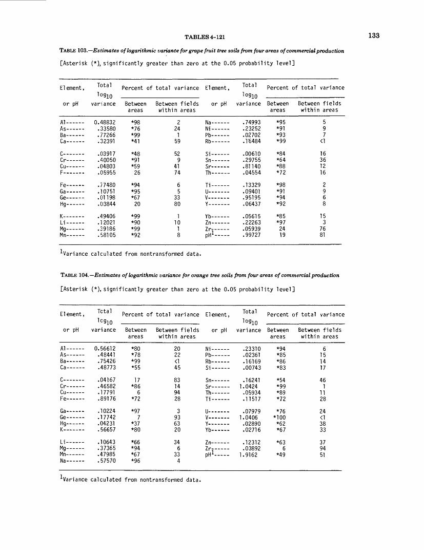
TABLES 4-121
TABLE 103.—Estimates of logarithmic variance for grape fruit tree soils from four areas of commercial production
[Asterisk (*), significantly greater than zero at the 0.05 probability level]
133
Element
or pH
Al__ __ _
A<:--__-D^
Ca —— -
r______O___ _Cu -----F ______
Fe — —Ga — -Ge —— -Hg— -
i/Li ——Mg — — Mn — —
Total percent of total variance Element, Total Percent of total variance Iog10 log in
variance
0 /IQQOO
'jocon
.77266
.32391
0391740050.0480305955
.77480
.10751rn i QP03844
.49406
.12021TQl P£
.58105
Between Between fields or pH areas within areas
*98 *76 *99 *41
*48 *91 *59 26
*94 *95 *67 20
*99 *90 *99 *92
2 24 1 59
52 9
41 74
6 5
33 80
1 10 1 8
Na- —— -Mi
Pb————— -Rb —— — -
Si ——— -Sn ——— •Cr___ __ .
Th— — -
Ti ——— .U —— — .V — ___.
Yb— — -Zn —— --Zr ——— .nH 1
variance Between Between fields areas within areas
.74993O OO CO
.02702
.16484
.00610 29755.81140 04554
.13329
.09401
.95195
.06437
.05615oooco
.05939
.99727
*95 *91 *93 *99
*84 *64 *88 *72
*98 *91 *94 *92
*85 *97 24 19
5 9 7
<1
16 36 12 16
2 9 6 8
15 3
76 81
•^Variance calculated from nontransformed data.
TABLE 104.— Estimates of logarithmic variance for orange tree soils from four areas of commercial production
[Asterisk (*), significantly greater than zero at the 0.05 probability level]
Element, ° a Percent of total variance Element log in
or pH
Al-----A<;--_--D^
Ca —— -
r_____.r r_ _ _.Cu —— -Fe——
Ga——Ge —— -Hg———
Li —— -Mg —— -Mn —— -Na
variance
•- 0.56612.48441.75426.48773
.04167
.46582
.17791
.89176
.10224
.17742
.0423156657
.10643O ~7O£ C
47985.57570
Between Between fields or pH areas within areas
*80 *78 *99 *55
17 *86
6 *72
*97 7
*37 *80
*66 *94 *67 *96
20 22 <1 45
83 14 94 28
3 93 63 20
34 6
33 4
Ni — —Pb — --Rb———Si — —
Sn -----
Th — —Ti- — —
U— - —V ______Y ————WL
Zn — —Zr ———pHl~~
TotalIo9l0
variance
23310.02361.16169.00743
.16241 - 1.0424
05934.11517
.079791.0406
nopon
.02716
• 1 -» \J 1 t-
038Q?- 1.9162
Percent of total variance
Between Between fields areas within areas
*94 *85 *86 *83
*54 *99 *89 *72
*76 *100 *62 *67
*63 6
*49
6 15 14 17
46 1
11 28
24 <138 33
37 94 51
Variance calculated from nontransformed data.

134 ELEMENTS IN FRUITS AND VEGETABLES, CONTERMINOUS UNITED STATES
TABLE 105.—Estimates of logarithmic variance for peach tree soils from four areas of commercialproduction
[Asterisk (*), significantly greater than zero at the 0.05 probability level]
Element
or pH
AT _ ___AC __ _ __
0 =
Ca———
Co— -
Cu ———F ———Fe ———Ga ———Ge———
Hg———V
Li ———Mg ———Mn ———
Total Percent of total variance Element, Tota1 Percent of log ]n log in
variance
- 0.01143.4137112445
.01718
.01874
.0256907039
.10809
.12634
.04201
.03476
.00679
.08956
00541.01616nco oom oco
total variance
Between Between fields or pH variance Between Between fields areas within areas areas within areas
*92 24
*74 *52
*99 *93 *92 *82
*80 *35 *98 M8
10
*34 *95 *89 *98 *73
8 76 26 48
1 7 8
18
20 65
2 52 90
66 5
11 2
27
Na —— -Nb —— -Ni —— - Pb —— -
Rb —— -Sc———Si —— -Sn —— -
Sr —— -Th —— -Ti —— - U ——— .V ——— -
Y ——— .Yb———Zn- — -Zr- — -pH
.03496
.00173
.10751o ncoo
nooQQ
.06174
.00157
.13744
.06615
.03564
.02140
.01669
.07018
.01030
.01026
.01784
.045651.2711
*99
*70 *71
*88 *96 *87
*83 *56 *95 *85 *89
3 *88
64 *78
1 100
30 29
12 4
13 100
17 44
5 15 11
100 97 12 36 22
•'•Variance calculated from nontransformed data.
TABLE 106.— Estimates of logarithmic variance for pear tree soils from five areas of commercialproduction
[Asterisk (*), significantly greater than zero at the 0.05 probability level]
Element
or pH
D ~
Be- —Ca— -—
Co———
O _ ---
F ————Fe- —Ga ———
Ge —— -Hg— -
Li ———Mg ———
Total percent of total variance Element, To Percent of total variance Iog 10 logm
variance
0.02789.11167
(TU44
.01353OOO. C1
.02746ncOOO
.09165O CO CO
.03985
.05604
.02920
.00920
.06017
.00362
.01735i nooi
Between Between fields or pH variance Between Between fields areas within areas areas within areas
*75 Ml *65 *59
19 *84 *71 *70
*78 *82 *62 *72 *69
22 23
MO M2 *92
25 59
41
81 16 29 30
2218 38 28 31
78 77 60 58
8
Mn ———
i\rPb —— -
pk
Si—— -Sn —— -
$r— — -Th ———
U ——— -V ——— -
Y ——— -vu
Zn —— -
ulp
n7O1 Q
.03247
.13258
.16003
.01879nQQQO
.00431
.07153
.09364noi on
.02175
.01406
.09047
n one o
nonon
D4903.04666
- 1.1833
16 *80 *73 *82
M3 *84 *79
4
*89
*72*85 *80
17 *83
*70
84 20 27 18
57 16 21 96
11 61 28 15 20
62 83 17
30
Variance calculated from nontransformed data.
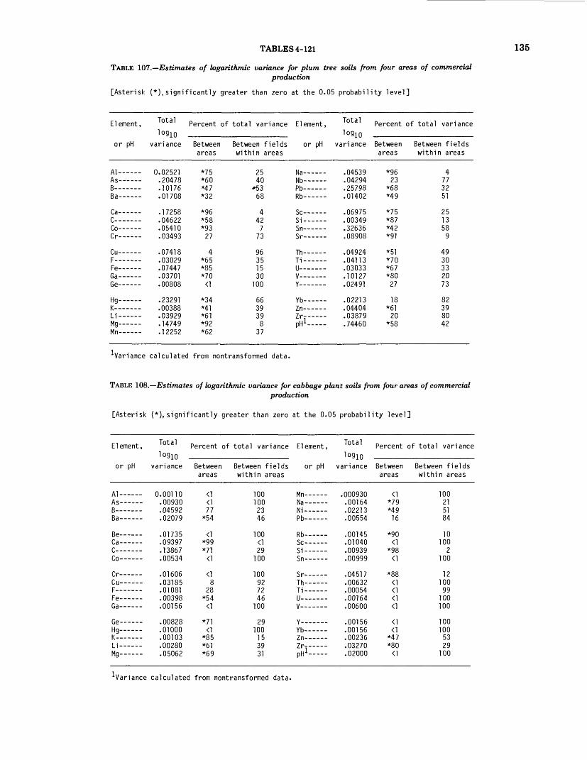
TABLES 4-121
TABLE 107.— Estimates of logarithmic variance for plum tree soils from four areas of commercialproduction
[Asterisk (*),significantly greater than zero at the 0.05 probability level]
135
Element
or pH
A1-- --A<-____
Da
Ca———r_ _ _Co—— -Q r _ _ __
Cu- —F- — —Fe — —Ga ———Ge —— -
Hg— -
Li — --Mg ———Mn ———
, Total Percent of Io 9l0
variance
0 02521.20478.10176.01708
1 7OCQ
.04622
.05410n?4Q?
.0741803029.07447.03701nnono
23291nnooo
D?Q?Q
.147491 o oc o
Between areas
*75 *60 *47 *32
*96 *58 *93 27
4 *65 *85 *70 <1
*34 Ml *61 *92 *62
total variance Element
Between fields or pH within areas
25 40
*53 68
4 42 7
73
96 35 15 30
100
66 39 39 8
37
Ma
Nb —— -Pb ——— -Rb —— •
Sc ——— -Si- —— •Sn ——— -<;»•
Th ——— -Ti ——— .U — ----V ——— -Y ———— .
Yb— —Zn— —zr_ — .
i pH 1 —— -
Total perCent of total variance login
variance Between Between fields areas within areas
.04539
.04294
.25798
.01402
.06975
.00349
.32636noono
.04924
.04113
.03033
.10127
.02491
02213.04404 .03879.74460
*96 23
*68 M9
*75 *87 M2 *91
*51 *70 *67 *80 27
18 *61 20
*58
4 77 32 51
25 13 58 9
49 30 33 20 73
82 39 80 42
Variance calculated from nontransformed data.
TABLE 108.— Estimates of logarithmic variance for cabbage plant soils from four areas of commercialproduction
[Asterisk (*), significantly greater than zero at the 0.05 probability level]
Element
or pH
A!--- _
D ̂
Be — —Ca— —T------Co ———
Cr--- _Cu———F —————Fe — --Ga — --
Ge — --Hg———
Li — —Mg — —
Total pe rcent of login
variance
- 0. 00110.0093004592.02079
.01735093971 *3QC 7
.00534
.01606
.03185
.0108100398.00156
nnooQ
.01000
.00103
.05062
Between areas
77 *54
*99 *71
8 28
*54
*71
*85 *61 *69
total variance Element
Between fields or pH within areas
100 100 23 46
100
29 100
100 92 72 46
100
29 100 15 39 31
Mn ———
Ni ———Pb — —
Rb ———Sc— —Si ———
Th — —Ti — —U ———V ———
Y ______Yb — —Zn — —
pH1 ——
Total percent of log in
total variance
variance Between Between fields areas within areas
.000930 <1.00164 *7902213 M900554 16
00145 *90.01040 <1
.00999 <1
04517 *88.00632 <1
.00164 <1
.00600 <1
.00156 <1
.00156 <100236 *47.03270 *80.02000 <1
100 21 51 84
10 100
2 100
12 100 99 100 100
100 100 53 29 100
Variance calculated from nontransformed data.
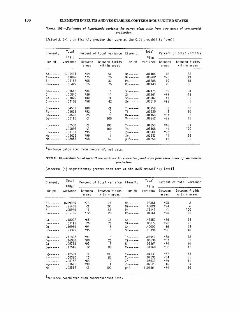
136 ELEMENTS IN FRUITS AND VEGETABLES, CONTERMINOUS UNITED STATES
TABLE 109.—Estimates of logarithmic variance for carrot plant soils from two areas of commercialproduction
[Asterisk (*), significantly greater than zero at the 0.05 probability level]
Element,
or pH
AT ______ _
Ac_ __ ___
Ca ———
Co ———Cr--- -- -
Cu ———Fe ———Ga ———Ge——— -
Hg———
Li ————Mg ———— Mn ————
Percent of total variance login
variance Between Between fields areas within areas
0.00494 *49 51 .01089 *75 25 .04152 *68 32 .00427 25 75
.03642 *84 16
.00840 *89 11
.01070 100 <1
.04102 *58 42
.04531 100 <1
.01025 *93 7
.00620 25 75
.00116 <1 100
.07538 <1 100
.00094 <1 100
.03181 *95 5
.06035 *99 1
.02852 *58 42
El ement
or pH
Na ———
Pb ———Rb ———
Sc ———Si ———Sn ———Sr ———
Th ———Ti ———U ————V- ——
Y ————Yb ———Zn ———
ofX—pn
Total Iog 10
variance
.01106
m 9QQ
.00143
.02175
.00161nocno
.07810
00959.00230.01168ncoco
.01855
.01108
.00681noooo
.04250
Percent
Between areas
18 *76
19 20
69 *88
*92
32 4
*97 *82
*46
*9241
of total variance
Between fields within areas
82 24 81 30
31 12
100 8
68 96
3 18
54 100
8 59
100
Variance calculated from nontransformed data.
TABLE 110.— Estimates of logarithmic variance for cucumber plant soils from three areas of commercial production
[Asterisk (*) significantly greater than zero at the 0.05 probability level]
Element,
or pH
AlAc_
R =
Ca— —
Co— —fV— — —
Cu———Fe ———Ga ———Ge ———
Hg———
Li ————Mg ————Mn ————
Percent of total variance log in
variance Between Between fields areas within areas
0.09025 *73 27 .25468 <1 100 .05926 15 85 .05766 *72 28
.18097 *65 35
.03111 25 75
.16969 *94 6
.29329 *95 5
.41802 *92 8
.16988 *80 20
.09788 *93 7
.17516 12 88
.12529 <1 100
.00320 13 87
.06157 *88 12
.33695 *99 1
.03524 <1 100
Element
or pH
Na ———
Pb ———Rb ———
Sc ———Si ———Sn ———Sr-- ---
Th———Ti ———U ———V ———
Y ———Yb ———Zn ———ZrpH 1 ——
Total
10910
variance
noo c i
.40021
.13147
.01661
47350.00877.40000.13196
.06940
.06636
.02364
.31960
04139.04633.05639
n ocoo
1.0296
Percent
Between areas
*94
*70
*86 *78
36 *90
*78 *67 *74 *88
*57 *64
16 *74
of total variance
Between fields within areas
2 6
100 30
14 22 64 10
22 33 26 12
43 36 11 84 26
Variance calculated from nontransformed data.
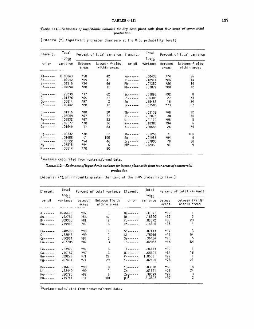
TABLES 4-121
TABLE III.—Estimates of logarithmic variance for dry bean plant soils from four areas of commercialproduction
[Asterisk (*), significantly greater than zero at the 0.05 probability level]
137
Element, Total Percent of log in
or pH
Al-----
D -»
Ca —— -C_ _ __.Co —— -Cr-----
Cu— -F ——— -Fe —— -Ga ——Ge —— -
Hg—— -i/Li —— -Mg —— -Mn —— -
variance
-- 0.030430395204315
.04094
.01376
.05814
.09442
.0131605059noc oo
.02577
.01649
m /IQQnriooonooi c
.06514
Between areas
*58 *59 *34 *88
*37 *65 *97 *88
*80 *67 *67 *70
17
*38
*54 *94 *70
total variance Element Total percent of log in
total variance
Between fields or pH variance Between Between fields within areas areas within areas
42 41 66 12
62 35
3 12
20 33 33 30 83
62 100 46
6 30
Ni ———Pb ———Rh
Sc ———Si —— -Sn ———
Th —— -Ti- — -U- ———V- ———Y ______
Yb ———Zn ———Zr —— -pHl--
• »J»J"OO
.18914
.01350
.01879
m QOQ
.00305
.15487
.01585
• \J\J I +JL.
.02075
.01120i mQ 1?
.00688
.01256
.01956
.079031.1205
*74 *86 *86 *88
*92 27 16
*73
*68 30
*95 *94
26
*94 70 91
26 14 14 12
8 73 84 27
32 70
5 6
74
100 6
30 9
Variance calculated from nontransformed data.
TABLE 112.—Estimates of logarithmic variance for lettuce plant soils from four areas of commercialproduction
[Asterisk (*), significantly greater than zero at the 0.05 probability level]
El ement
or pH
A!--- -
Ca ———C------Cr-----Cu— — -
Fe— —Ga —— -Ge———Hg-—
V
Li ———Mg ——— Mn ———
, Total Percent of Io 9l0 - -
variance
0.4649542754
.09360
.19965
48509.53046.50964.07706
.10157
.29278
.07431
.16636
.22449on~7o/-
.19744
Between areas
*97 *58 *81 *82
*90 *99 *97 *87
*92 *97 *71 *71
*90 *99 *92
total variance Element, Total Percent of total variance log in
Between fields or pH variance Between Between fields within areas areas within areas
3 42 19 18
10 1 3
13
8 3
29 29
10 1 8
100
Na —— -
Pb----PK
Sc— —Si —— -Sr— — -
Ti —— -U ——— .V ——— -Y- —— .
Yb—— -Zn- — -7.-
pH 1 ——
.31041i QQ/I nno c 70
.14806
.07113
.7501636484
.02063
.34473
.055051.0502
.02695
.03038
.01361
.38599
*99 *97 *80 *96
*97 *46 *95 *46
*99 *84 *99 *78
*82 *76 *97 *97
1 3
204
3 54
5 54
1 16
1 21
18 24
33
^Variance calculated from nontransformed data.
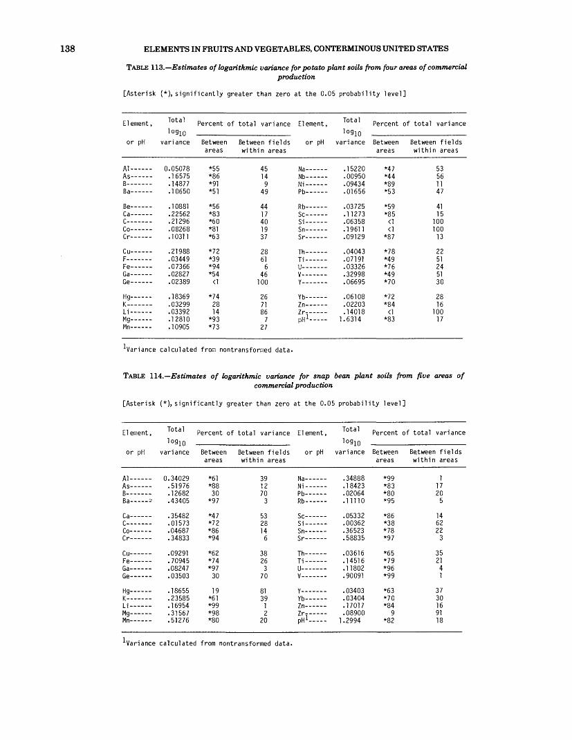
138 ELEMENTS IN FRUITS AND VEGETABLES, CONTERMINOUS UNITED STATES
TABLE 113.—Estimates of logarithmic variance for potato plant soils from four areas of commercialproduction
[Asterisk (*), significantly greater than zero at the 0.05 probability level]
Element, Total Percent of login
or pH
Al-----Ac _ __.
D -!
Be —— -Ca- — -Q_ _ __.
Co- — -Qr __ _.
Cu- ——F ——— .Fe —— -Ga— -Ge —— -
Hg— -I/
Li— ..Mg —— - Mn —— -
variance
•- 0.05078.16575.14877.10650
i nppi99 C£9
91 9G£
HQ9£Q
.10311
91 QPQ
.03449
.07366H9Q97
n9TQQ
.18369
.03299
.03392i 9Pi n
.10905
Between areas
*55 *86 *91 *51
*56 *83 *60 *81 *63
*72 *39 *94 *54
<1
*74 28 14
*93 *73
total variance Element
Between fields or pH within areas
45 14
9 49
44 17 40 19 37
28 61
6 46
100
26 71 86
7 27
Ma
Nb ———Ni ——— Pb — --
Rb ———Sc ———Si- — -Sn — --
Th ———Ti- — -U ———V ———Y —— --
WL
Zn — --
nH 1
Total Percent of log in
total variance
variance Between Between fields areas within areas
l ti??0.00950.09434.01656
.03725
.11273
.06358
.19611
.09129
.04043
.07191HQQ 9£
32998.06695
.0610802203
.14018- 1.6314
*47 *44 *89 *53
*59 *85
<1 <1
*87
*78 *49 *76 *49 *70
*72 *84
<1 *83
53 56 11 47
41 15
100 100
13
22 51 24 51 30
28 16
100 17
Variance calculated from nontransformed data.
TABLE 114.— Estimates of logarithmic variance for snap bean plant soils from five areas ofcommercial production
[Asterisk (*), significantly greater than zero at the 0.05 probability level]
Element
or pH
/\1__ _AQ-----
D -,
Ca ———r------Co ———
Cu- ——Fe ———Ga ———Ge ———
Hg— -I/
Li ——Mg ——— Mn ———
Percent of total variance Element Io9l0
variance
0 34029.51976
1 9£Q9
- 43405
O C>l Q9
.01573
.04687
.34833
.0929170945
.08247r\ o cno
.186559O COC
.16954
.31567
.51276
Between Between fields or pH areas within areas
*61 *88 30
*97
*47 *72 *86 *94
*62 *74 *97
30
19 *61 *99 *98 *80
39 12 70
3
53 28 14
6
38 26
3 70
81 39
1 2
20
Ma
Ni ———Pb— —Rb ———
Si ———Sn-- —
Th-- —Ti ———U— - —V ———
Y ———WL
Zn ———i pH 1 ——
Total percent O f total variance log in
variance Between Between fields areas within areas
O>l QQQ
184?"}.02064.11110
.05332
.00362OC C. 9O
.58835
.03616
.145161 1 QH9
.90091
.0340303404
.17017
.08900- 1.2994
*99 *83 *80 *95
*86 *38 *78 *97
*65 *79 *96 *99
*63 *70 *84
9 *82
1 17 20
5
14 62 22
3
35 21
4 1
37 30 16 91 18
Variance calculated from nontransformed data.

TABLES 4-121
TABLE 115.—Estimates of logarithmic variance for sweet corn plant soils from four areas of commercialproduction
[Asterisk (*), significantly greater than zero at the 0.05 probability level]
139
El ement
or pH
Al-----Ac_--"--
Ra
Ca ———r______
o_ _ __Cu -----Fe-- —Ge———
Hg— -K _ ____Li ———Mg ———
, ° a Percent of total variance Element Iog10
variance
0 3824495358Dfi?^
.54677
.60874
.09787
3329002599OCOO 7
0133?
.07149TQOQO
1 O 1 CO
38484
Between Between fields or pH areas within areas
*95 *93
<1
*98 *98 *78
*72 *45 *99 *52
19 *98 *97 *99
5 7
100
2 2
22
28 55
1 48
81 2 3 1
Mn ———Pb ———Dk
Si ———Sn ———
Th ———Ti- ——U ———V ———
Yb———In— —Zr ———int-HpH - ——
Total Percent of total variance Iog 10
variance Between Between fields areas within areas
.04202
.10132
.00715
.02705
.64710
.047851 ft"39fi
.10631
.057161 1 OCO
- 1.1340
*91 *76 *97
*85 *52 *97
*81 *93 *96 *99
*60 *81 *64 *81
9 24
3
15 48
3
19 7 4 1
40 19 36 19
•^Variance calculated from nontransformed data.
TABLE 116.—Estimates of logarithmic variance for tomato plant soils from five areas of commercial production
[Asterisk (*\ significantly greater than zero at the 0.05 probability level]
Element
or pH
Al---_-
Ca ———
Co -----
Cu — --
Fe ———Ga ———Ge ———Hg———
Li _____Mg — — Mn — —
, ° Percent of total variance Element, Total Percent of total variance Iog 10 logm
variance
0.42696.50817.47679.29205
.02994no/i DD35009
.10965
.85356
.1007001059
.08157
27377.09394.30517.21456
Between Between fields or pH variance Between Between fields areas within areas areas within areas
*99 *71 *96 *99
*76 *88 *81 *79
*99 *97 *64 *44
*99 *98 *99 *91
29 4 1
24 12 19 21
3 36 56
2
9
Ni —— -
Rb— ——
Si —— -Sn —— -
Th —— -
Ti —— -U ——— .V ——— .Y ——— .
vu.
Zn—— -Zr— -pH 1 - —
01Q7Q
.04028
.072641 "39T3
.00612
.31586OCO7O
.06564
.19651
.92649
.05602
.07066ncnoo
.06940i i fti ft
*85 *40 *99 *93
*91 *58 *99 *86
*99 *96 *99 *82
*79 *96 *51 *70
15 60
1 7
9 42
1 14
14 1
18
214
49 30
^Variance calculated from nontransformed data.
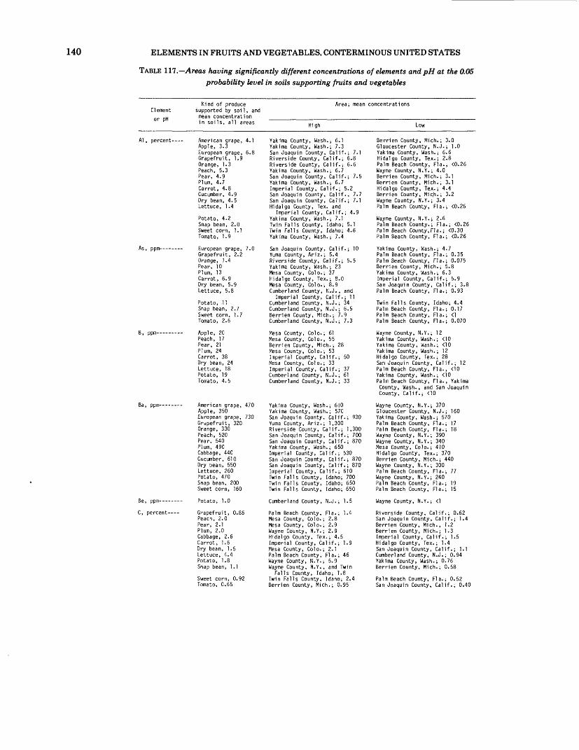
140 ELEMENTS IN FRUITS AND VEGETABLES, CONTERMINOUS UNITED STATES
TABLE 117.— Areas having significantly different concentrations of elements and pH at the 0.05 probability level in soils supporting fruits and vegetables
Element or pH
Kind of produce supported by soi1, and mean concentration in soils, all areas
Area; mean concentrations
High Low
Al, percent----
As, ppm--
B, ppm-
Ba, ppm--
Be, ppm----
C, percent-
American grape, 4.1 Apple, 3.3 European grape, 6.8 Grapefruit, 1,9 Orange, 1.3 Peach, 5.3 Pear, 4.9 Plum, 4.7 Carrot, 4.8 Cucumber, 4.9 Dry bean, 4.5 Lettuce, 1.4
Potato, 4.2 Snap bean, 2.0 Sweet corn, 1.1 Tomato, 1.9
European grape, 7.0 Grapefruit, 2.2 Orange, 1.4 Pear, 10 Plum, 13 Carrot, 6.9 Dry bean, 5.9 Lettuce, 5.8
Potato, .11 Snap bean, 2.7 Sweet corn, 1.7 Tomato, 2.6
Apple, 20 Peach, 17 Pear, 21 Plum, 24 Carrot, 38 Dry bean, 24 Lettuce, 18 Potato, 19 Tomato, 4.5
American grape, 470 Apple, 350 European grape, 730 Grdpefruit, 320 Orange, 330 Peach, 520 Pear, 540 Plum, 490 Cabbage, 440 Cucumber, 610 Dry bean, 550 Lettuce, 260 Potato, 470 Snap bean, 200 Sweet corn, 160
Potato, 1.0
Grapefruit, 0.86 Peach, 2.0 Pear, 2.1 Plum, 2.0 Cabbage, 2.6 Carrot, 1.6 Dry bean, 1.5 Lettuce, 4.4 Potato, 1.8 Snap bean, 1.1
Sweet corn, 0.92 Tomato, 0.65
Yakima County, Wash.; 6.1 Yakima County, Wash.; 7.3 San Joaquin County, Calif.; 7.1 Riverside County, Calif.; 6.8 Riverside County, Calif.; 6.6 Yakima County, Wash.; 6.7 San Joaquin County, Calif.; 7.5 Yakima County, Wash.; 6.7 Imperial County, Calif.; 5.2 San Joaquin County, Calif., 7.7 San Joaquin County, Calif.; 7.1 Hidalgo County, Tex. and
Imperial County, Calif.; 4.9 Yakima County, Wash.; 7.1 Twin Falls County, Idaho; 5.1 Twin Falls County, Idaho; 4.6 Yakima County, Wash.; 7.4
San Joaquin County, Calif.; 10 Yuma County, Ariz.; 5.4 Riverside County, Calif.; 5.5 Yakima County, Wash.; 23 Mesa County, Colo.; 37 Hidalgo County, Tex.; 8.0 Mesa County, Colo.; 8.9 Cumberland County, N.J., and
Imperial County, Calif.; 11 Cumberland County, N.J.; 34 Cumberland County, N.J.; 6.5 Berrien County, Mich.; 7.9 Cumberland County, N.J.; 7.3
Mesa County, Colo.; 61 Mesa County, Colo., 55 Berrien County, Mich.; 28 Mesa County, Colo.; 53 Imperial County, Calif.; 50 Mesa County, Colo.; 33 Imperial County, Calif.; 37 Cumberland County, N.J.; 61 Cumberland County, N.J.; 33
Yakima County, Wash.; 610 Yakima County, Wash.; 570 San Joaquin County, Calif.; 930 Yuma County, Ariz.; 1,300 Riverside County, Calif.; 1,300 San Joaquin County, Calif-; 700 San Joaquin County, Calif.; 870 Yakima County, Wash.; 650 Imperial County, Calif.; 530 San Joaquin County, Calif.; 870 San Joaquin County, Calif.; 870 Imperial County, Calif.; 610 Twin Falls County, Idaho; 700 Twin Falls County, Idaho; 650 Twin Falls County, Idaho; 650
Cumberland County, N.J.; 1.5
Palm Beach County, Fla.; 1.4 Mesa County, Colo.; 2.8 Mesa County, Colo.; 2.9 Wayne County, N.Y.; 2.9 Hidalgo County, Tex.; 4.5 Imperial County, Calif.; 1.9 Mesa County, Colo.; 2.1 Palm Beach County, Fla.; 46 Wayne County, N.Y.; 5.9 Wayne County, N.Y., and Twin
Falls County, Idaho; 1.8 Twin Falls County, Idaho; 2.4 Berrien County, Mich.; 0.95
Berrien County, Mich.; 3.0 Gloucester County, N.J.; 1.0 Yakima County, Wash.; 6.6 Hidalgo County, Tex.; 2.8 Palm Beach County, Fla.; <0.26 Wayne County, N.Y.; 4.0 Berrien County, Mich.; 3.1 Berrien County, Mich.; 3.1 Hidalgo County, Tex.; 4.4 Berrien County, Micji.; 3.2 Wayne County, N.Y.; 3.4 Palm Beach County, Fla.; <0.26
Wayne County, N.Y.; 2.6 Palm Beach County.; Fla.; <0.26 Palm Beach County,Fla.; <0.30 Palm Beach County, Fla.; <0.26
Yakima County, Wash.; 4.7 Palm Beach County, Fla.; 0.35 Palm Beach County, Fla.; 0.075 Berrien County, Mich.; 5.8 Yakima County, Wash.; 6.3 Imperial County, Calif.; 5.9 San Joaquin County, Calif.; 3.8 Palm Beach County, Fla.; 0.93
Twin Falls County, Idaho; 4.4Palm Beach County, Fla.; 0.17Palm Beach County, Fla.; <1Palm Beach County, Fla.; 0.070
Wavne County, N.Y.; 12 Yakima County, Wash.; <10 Yakima County, Wash.; <10 Yakima County, Wash.; 12 Hidalgo County, Tex.; 28 San Joaquin County, Calif.; 12 Palm Beach County, Fla., <10 Yakima County, Wash.; <10 Palm Beach County, Fla., YakimaCounty, Wash., and San JoaquinCounty, Calif.; <10
Wayne County, N.Y.; 370 Gloucester County, N.J.; 160 Yakima County, Wash.; 570 Palm Beach County, Fla.; 17 Palm Beach County, Fla.; 18 Wayne County, N.Y.; 390 Wayne County, N.Y.; 340 Mesa County, Colo.; 410 Hidalgo County, Tex.; 370 Berrien County, Mich.; 440 Wayne County, N.Y.; 300 Palm Beach County, Fla.; 77 Wayne County, N.Y.; 240 Palm Beach County, Fla.; 19 Palm Beach County, Fla.; 15
Wayne County, N.Y.; <1
Riverside County, Calif.; 0.62 San Joaquin County, Calif.; 1.4 Berrien County, Mich., 1.2 Berrien County, Mich.; 1.3 Imperial County, Calif.; 1.5 Hidalgo County, Tex.; 1.4 San Joaquin County, Calif.; 1.1 Cumberland County, N.J.; 0.94 Yakima County, Wash.; 0.76 Berrien County, Mich.; 0.58
Palm Beach County, Fla.; 0.52 San Joaquin County, Calif.; 0.40
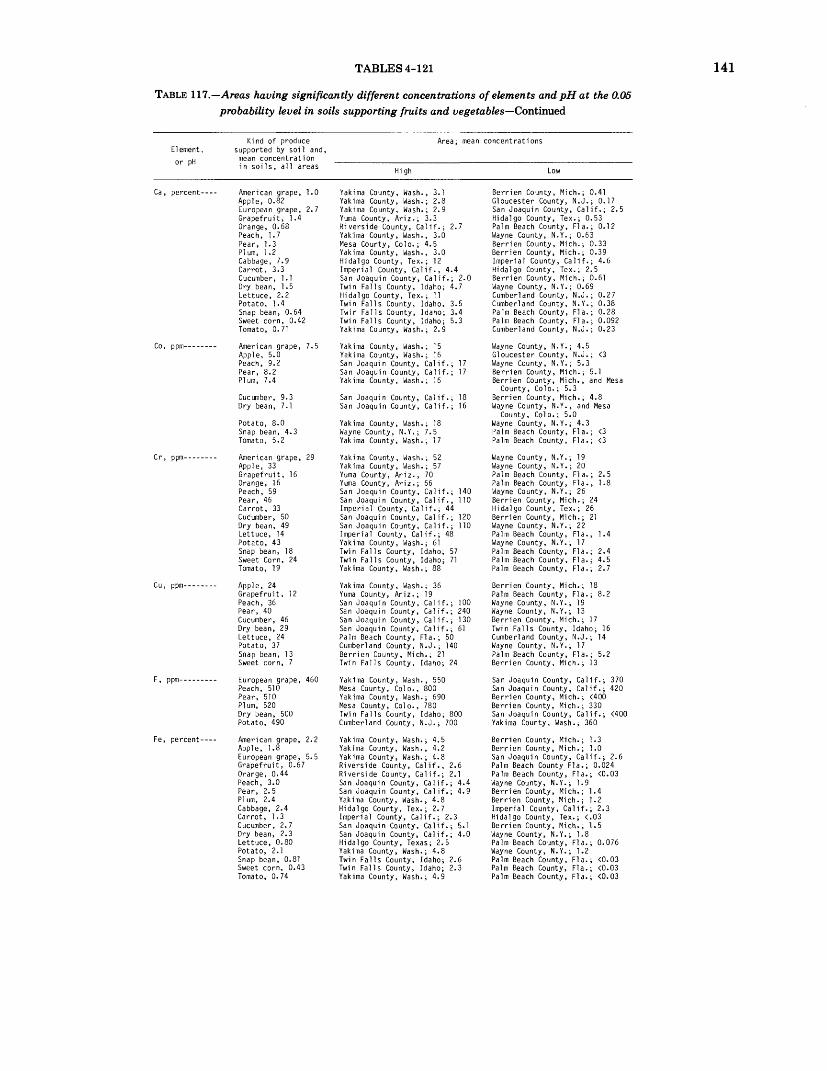
TABLES 4-121 141
TABLE 111.—Areas having significantly different concentrations of elements and pH at the 0.05 probability level in soils supporting fruits and vegetables—Continued
Element,Kind of produce
supported by soil and,mean concentrationin soils, all areas
Area; mean concentrations
High Low
Ca, percent----
Co, ppm-
Cr, ppm-
Cu, ppm-
F, ppm-
Fe, percent----
American grape, 1.0 Apple, 0.82 European grape, 2.7 Grapefruit, 1.4 Orange, 0.68 Peach, 1.7 Pear, 1.3 Plum, 1.2 Cabbage, 7.9 Carrot, 3.3 Cucumber, 1.1 Dry bean, 1.5 Lettuce, 2.2 Potato, 1.4 Snap bean, 0.64 Sweet corn, 0.42 Tomato, 0.71
American grape, 7.5 Apple, 5.0 Peach, 9.2 Pear, 8.2 Plum, 7.4
Cucumber, 9.3 Dry bean, 7.1
Potato, 8.0 Snap bean, 4.3 Tomato, 5.2
American grape, 29 Apple, 33 Grapefruit, 16 Orange, 16 Peach, 59 Pear, 46 Carrot, 33 Cuc'umber, 50 Dry bean, 49 Lettuce, 14 Potato, 43 Snap bean, 18 Sweet Corn, 24 Tomato, 19
Apple, 24 Grapefruit, 12 Peach, 36 Pear, 40 Cucumber, 46 Dry bean, 29 Lettuce, 24 Potato, 37 Snap bean, 13 Sweet corn, 7
European grape, 460 Peach, 510 Pear, 510 Plum, 520 Dry bean, 500 Potato, 490
American grape, 2.2 Apple, 1.8 European grape, 5.5 Grapefruit, 0.67 Orange, 0.44 Peach, 3.0 Pear, 2.5 Plum, 2.4 Cabbage, 2.4 Carrot, 1.3 Cucumber, 2.7 Dry bean, 2.3 Lettuce, 0.80 Potato, 2.1 Snap bean, 0.81 Sweet corn, 0.43 Tomato, 0.74
Yakima County, Wash., 3.1 Yakima County, Wash.; 2.8 Yakima County, Wash.; 2.9 Yuma County, Ariz.; 3.3 Riverside County, Calif.; 2.7 Yakima County, Wash., 3.0 Mesa County, Colo.; 4.5 Yakima County, Wash., 3.0 Hidalgo County, Tex.; 12 Imperial County, Calif., 4.4 San Joaquin County, Calif.; 2.0 Twin Falls County, Idaho; 4.7 Hidalgo County, Tex.; 11 Twin Falls County, Idaho, 3.5 Twin Falls County, Idaho; 3.4 Twin Falls County, Idaho; 5.3 Yakima County, Wash.; 2.9
Yakima County, Wash.; 15 Yakima County, Wash.; 16 San Joaquin County, Calif.; 17 San Joaquin County, Calif.; 17 Yakima County, Wash.; 16
San Joaquin County, Calif.; 18 San Joaquin County, Calif.; 16
Yakima County, Wash.; 18 Wayne County, N.Y.; 7.5 Yakima County, Wash.; 17
Yakima County, Wash.; 52 Yakima County, Wash.; 57 Yuma County, Ariz., 70 Yuma County, Ariz.; 66 San Joaquin County, Calif.; 140 San Joaquin County, Calif., 110 Imperial County, Calif.; 44 San Joaquin County, Calif.; 120 San Joaquin County, Calif.; 110 Imperial County, Calif.; 48 Yakima County, Wash.; 61 Twin Falls County, Idaho; 57 Twin Falls County, Idaho; 71 Yakima County, Wash.; 88
Yakima County, Wash.; 36 Yuma County, Ariz.; 19 San Joaquin County, Calif.; 100 San Joaquin County, Calif.; 240 San Joaquin County, Calif.; 130 San Joaquin County, Calif.; 61 Palm Beach County, Fla.; 50 Cumberland County, N.J.; 140 Berrien County, Mich.; 21 Twin Falls County, Idaho; 24
Yakima County, Wash., 550 Mesa County, Colo., 800 Yakima County, Wash.; 690 Mesa County, Colo., 780 Twin Falls County, Idaho; 800 Cumberland County, N.J.; 700
Yakima County, Wash.; 4.5 Yakima County, Wash., 4.2 Yakima County, Wash.; 4.8 Riverside County, Calif., 2.6 Riverside County, Calif.; 2.1 San Joaquin County, Calif.; 4.4 San Joaquin County, Calif.; 4.9 Yakima County, Wash., 4.8 Hidalgo County, Tex.; 2.7 Imperial County, Calif.; 2.3 San Joaquin County, Calif.; 5.1 San Joaquin County, Calif.; 4.0 Hidalgo County, Texas; 2.5 Yakima County, Wash.; 4.8 Twin Falls County, Idaho; 2.6 Twin Falls County, Idaho; 2.3 Yakima County, Wash.; 4.9
Berrien County, Mich.; 0.41 Gloucester County, N.J.; 0.17 San Joaquin County, Calif.; 2.5 Hidalgo County, Tex.; 0.53 Palm Beach County, Fla.; 0.12 Wayne County, N.Y.; 0.63 Berrien County, Mich.; 0.33 Berrien County, Mich.; 0.39 Imperial County, Calif.; 4.6 Hidalgo County, Tex.; 2.5 Berrien County, Mich.; 0.61 Wayne County, N.Y.; 0.69 Cumberland County, N.J.; 0.27 Cumberland County, N.Y.; 0.38 Palm Beach County, Fla.; 0.28 Palm Beach County, Fla.; 0.092 Cumberland County, N.J.; 0.23
Wayne County, N.Y.; 4.5 Gloucester County, N.J.; <3 Wayne County, N.Y.; 5.3 Berrien County, Mich.; 5.1 Berrien County, Mich., and Mesa
County, Colo.; 5.3 Berrien County, Mich.; 4.8 Wayne County, N.Y., and Mesa
County, Colo.; 5.0 Wayne County, N.Y.; 4.3 Palm Beach County, Fla.; <3 Palm Beach County, Fla.; <3
Wayne County, N.Y.; 19 Wayne County, N.Y.; 20 Palm Beach County, Fla.; 2.5 Palm Beach County, Fla., 1.8 Wayne County, N.Y.; 26 Berrien County, Mich.; 24 Hidalgo County, Tex.; 26 Berrien County, Mich.; 21 Wayne County, N.Y.; 22 Palm Beach County, Fla., 1.4 Wayne County, N.Y.; 17 Palm Beach County, Fla.; 2.4 Palm Beach County, Fla.; 4.5 Palm Beach County, Fla.; 2.7
Berrien County, Mich.; 18 Palm Beach County, Fla.; 8.2 Wayne County, N.Y.; 19 Wayne County, N.Y.; 13 Berrien County, Mich.; 17 Twin Falls County, Idaho; 16 Cumberland County, N.J.; 14 Wayne County, N.Y.; 17 Palm Beach County, Fla.; 5.2 Berrien County, Mich.; 13
San Joaquin County, Calif.; 370 San Joaquin County, Calif.; 420 Berrien County, Mich.; <400 Berrien County, Mich.; 330 San Joaquin County, Calif.; <400 Yakima County, Wash.; 360
Berrien County, Mich.; 1.3 Berrien County, Mich.; 1.0 San Joaquin County, Calif.; 2.6 Palm Beach County Fla.; 0.024 Palm Beach County, Fla.; <0.03 Wayne County, N.Y.; 1.9 Berrien County, Mich.; 1.4 Berrien County, Mich.; 1.2 Imperial County, Calif.; 2.3 Hidalgo County, Tex.; <.03 Berrien County, Mich.; 1.5 Wayne County, N.Y.; 1.8 Palm Beach County, Fla.; 0.076 Wayne County, N.Y.; 1.2 Palm Beach County, Fla.; <0.03 Palm Beach County, Fla.; <0.03 Palm Beach County, Fla.; <0.03
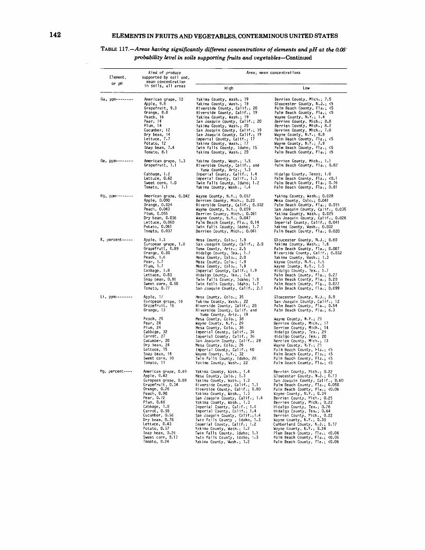
142 ELEMENTS IN FRUITS AND VEGETABLES, CONTERMINOUS UNITED STATES
TABLE 117.— Areas having significantly different concentrations of elements and pH at the 0.05' probability level in soils supporting fruits and vegetables—Continued
Element, or pH
Ga, ppm--- — —
Ge, ppm — -----
Hg, ppm —————
K, percent ———
Li, ppm —————
Mg, percent- —
Kind of produce supported by soil and,
mean concentration in soils, all areas
American grape, 12Apple, 9.8Grapefruit, 9.3Orange, 8.8Peach, 16Pear, 14Plum, 14Cucumber, 12Dry bean, 14Lettuce, 7.7Potato, 12Snap bean, 7.4Tomato, 8.1
American grape, 1.3Grapefruit, 1.1
Cabbage, 1.2Lettuce, 0.62Sweet corn, 1.0Tomato, 1.1
American grape, 0.042 Apple, 0.090Orange, 0.024Peach, 0.043Plum, 0.055Dry bean, 0.036Lettuce, 0.060Potato, 0.061Tomato, 0.037
Apple, 1.3 European grape, 1.8Grapefruit, 0.99Orange, 0.80Peach, 1.6Pear, 1.7Plum, 1.7Cabbage, 1.8Lettuce, 0.83Snap bean, 0.91Sweet corn, 0.58Tomato, 0.77
Apple, 17 European grape, 16Grapefruit, 16Orange, 13
Peach, 25Pear, 24Plum, 24Cabbage, 32Carrot, 27Cucumber, 20Dry bean, 24Lettuce, 15Snap bean, 14Sweet corn, 10Tomato, 11
American grape, 0.49Apple, 0.42European grape, 0.89Grapefruit, 0.34Orange, 0.26Peach, 0.90Pear, 0.72Plum, 0.66Cabbage, 1.0Carrot, 0.98Cucumber, 0.56Dry bean, 0.78Lettuce, 0.43Potato, 0.57Snap bean, 0.24Sweet corn, 0.17Tomato, 0.24
Area; mean
High
Yakima County, Wash.; 19Yakima County, Wash.; 19Riverside County, Calif.; 20Riverside County, Calif.; 19Yakima County, Wash.; 19San Joaquin County, Calif.; 20Yakima County, Wash.; 20San Joaquin County, Calif.; 19San Joaquin County, Calif.; 19Imperial County, Calif.; 17Yakima County, Wash.; 17Twin Falls County, Idaho; 15Yakima County, Wash.; 20
Yakima County, Wash.; 1.5Riverside County, Calif., and
Yuma County, Ariz.; 1.3Imperial County, Calif.; 1.4Imperial County, Calif.; 1.3Twin Falls County, Idaho; 1.2Yakima County, Wash.; 1.4
Wayne County, N.Y.; 0.057 Berrien County, Mich.; 0.23Riverside County, Calif.; 0.032Wayne County, N.Y.; 0.059Berrien County, Mich.; 0.061Wayne County, N.Y.; 0.047Palm Beach County, Fla.; 0.14Twin Falls County, Idaho; 1.7Berrien County, Mich.; 0.061
Mesa County, Colo.; 1.9 San Joaquin County, Calif.; 2.0Yuma County, Ariz.; 2.5Hidalgo County, Tex. ; 1.7Mesa County, Colo.; 2.0Mesa County, Colo. ; 1.9Mesa County, Colo.; 1.9Imperial County, Calif.; 1.9Hidalgo County, Tex.; 1.8Twin Falls County, Idaho; 1.8Twin Falls County, Idaho; 1.7San Joaquin County, Calif.; 2.1
Mesa County, Colo.; 35 Yakima County, Wash.; 22Riverside County, Calif.; 28Riverside County, Calif, and
Yuma County, Ariz.; 19Mesa County, Colo. ; 38Wayne County, N.Y.; 29Mesa County, Colo. ; 36Imperial County, Calif.; 34Imperial County, Calif.; 36San Joaquin County, Calif.; 29Mesa County, Colo. ; 26Imperial County, Calif.; 40Wayne County, N.Y. ; 32Twin Falls County, Idaho; 26Yakima County, Wash.; 22
Yakima County, Wash.; 1.4Mesa County, Colo. ; 1.3Yakima County, Wash.; 1.3Riverside County, Calif.; 1.1Riverside County, Calif.; 0.80Yakima County, Wash.; 1.3San Joaquin County, Calif.; 1.4Yakima County, Wash.; 1.3Imperial County, Calif.; 1.4Imperial County, Calif.; 1.4San Joaquin County, Calif.;!. 4Twin Falls County , Idaho, 1.3Imperial County, Calif.; 1.2Yakima County, Wash.; 1.2Twin Falls County, Idaho; 1.1Twin Falls County, Idaho; 1.3Yakima County, Wash.; 1.2
concentrations
Low
Berrien County, Mich.; 7.5Gloucester County, N.J.; <5Palm Beach County, Fla.; <5Palm Beach County, Fla.; <5Wayne County, N.Y.; 1.4Berrien County, Mich.; 8.8Berrien County, Mich.; 8.2Berrien County, Mich.; 7.0Wayne County, N.Y.; 8.8Palm Beach County, Fla.; <5Wayne County, N.Y.; 7.9Palm Beach County, Fla.; <5Palm Beach County, Fla.; <5
Berrien County, Mich.; 1.1Palm Beach County, Fla.; 0.82
Hidalgo County, Texas; 1.0Palm Beach County, Fla.; <0.1Palm Beach County, Fla.; 0.76Palm Beach County, Fla.; 0.81
Yakima County, Wash.; 0.028 Mesa County, Colo.; 0.041Palm Beach County, Fla.; 0.015San Joaquin County, Calif.; 0.035Yakima County, Wash.; 0.025San Joaquin County, Calif.; 0.026Imperial County, Calif.; 0.041Yakima County, Wash.; 0.032Palm Beach County, Fla.; 0.020
Gloucester County, N.J.; 0.60 Yakima County, Wash.; 1.6Palm Beach County, Fla.; 0.087Riverside County, Calif.; 0.032Yakima County, Wash.; 1.3Wayne County, N.Y.; 1.5Wayne County, N.Y.; 1.5Hidalgo County, Tex.; 1.7Palm Beach County, Fla.; 0.27Palm Beach County, Fla.; 0.20Palm Beach County, Fla., 0.077Palm Beach County, Fla.; 0.099
Gloucester County, N.J.; 8.9 San Joaquin County, Calif.; 12Palm Beach County, Fla.; 0.54Palm Beach County, Fla.; 6.3
Wayne County, N.Y.; 21Berrien County, Mich.; 17Berrien County, Mich.; 14Hidalgo County, Tex.; 29Hidalgo County, Tex. ; 20Berrien County, Mich.; 13Wayne County, N.Y.; 21Palm Beach County, Fla.; <5Palm Beach County, Fla.; <5Palm Beach County, Fla.; <5Palm Beach County, Fla.; <5
Berrien County, Mich.; 0.22Gloucester County, N.J.; 0.13San Joaquin County, Calif.; 0.60Palm Beach County, Fla.; 0.058Palm Beach County, Fla.; <0.06Wayne County, N.Y.; 0.39Berrien County, Mich.; 0.25Berrien County, Mich.; 0.22Hidalgo County, Tex.; 0.76Hidalgo County, Tex.; 0.64Berrien County, Mich., 0.22Wayne County, N.Y.; 0.30Cumberland County, N.J.; 0.17Wayne County, N.Y.; 0.24Plam Beach County, Fla.; <0.06Palm Beach County, Fla.; <0.06Palm Beach County, Fla.; <0.06
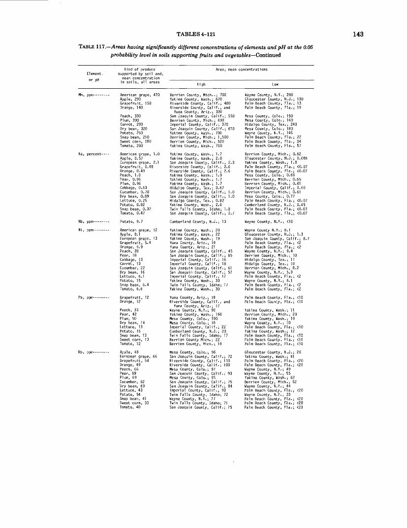
TABLES 4-121
TABLE 117.— Areas having significantly different concentrations of elements andpH at the 0.05 probability level in soils supporting fruits and vegetables—Continued
143
Element, or pH
Mn, ppm---- — —
Na, percent ——
Nb, ppm--- — ---
Ni , ppm- — — --
Pb, ppm--- —— -
Rb, ppm-- — — --
Kind of produce supported by soil and,
mean concentration in soils, all areas
American grape, 470Apple, 290Grapefruit, 150Orange, 140
Peach, 330Plum, 390Carrot, 290Dry bean, 320Potato, 250Snap bean, 210Sweet corn, 180Tomato, 280
American grape, 1.0Apple, 0.57European grape, 2.1Grapefruit, 0.48Orange, 0.49Peach, 1.0Pear, 0.96Plum, 0.96Cabbage, 0.63Cucumber, 0.78Dry bean, 0.89Lettuce, 0.25Potato, 0.82Snap bean, 0.32Tomato, 0.47
Potato, 9.7
American grape, 12Apple, 8.1European grape, 13Grapefruit, 5.4Orange, 5.9Peach, 20Pear, 18Cabbage, 13Carrot, 13Cucumber, 22Dry bean, 16Lettuce, 6.1Potato, 15Snap bean, 6.4Tomato, 6.6
Grapefruit, 12Orange, 12
Peach, 33Pear, 42Plum, 50Dry bean, 14Lettuce, 13Potato, 15Snap bean, 13Sweet corn, 13Tomato, 12
Apple, 49European grape, 66Grapefruit, 54Orange, 49Peach, 66Pear, 69Plum, 69Cucumber, 62Dry bean, 69Lettuce, 43Potato, 54Snap bean, 41Sweet corn, 33Tomato, 40
Area; mean
High
Berrien County, Mich..; 700Yakima County, Wash.; 670Riverside County, Calif.; 480Riverside County, Calif., and
Yuma County, Ariz.; 330San Joaquin County, Calif.; 550Berrien County, Mich.; 690Imperial County, Calif.; 370San Joaquin County, Calif.; 610Yakima County, Wash.; 700Berrien County, Mich.; 1,500Berrien County, Mich.; 520Yakima County, Wash.; 700
Yakima County, Wash.; 1.7Yakima County, Wash.; 2.0San Joaquin County, Calif.; 2.3Riverside County, Calif.; 2.6Riverside County, Calif.; 2.6Yakima County, Wash.; 1.9Yakima County, Wash.; 1.7Yakima County, Wash.; 1.7Hidalgo County, Tex.; 0.67San Joaquin County, Calif.; 1.0San Joaquin County, Calif.; 1.0Hidalgo County, Tex.; 0.82Yakima County, Wash.; 2.0Twin Falls County, Idaho; 1.0San Joaquin County, Calif.; 2.7
Cumberland County, N.J.; 13
Yakima County, Wash.; 20Yakima County, Wash.; 22Yakima County, Wash.; 19Yuma County, Ariz.; 19Yuma County, Ariz.; 21San Joaquin County, Calif.; 45San Joaquin County, Calif.; 65Imperial County, Calif.; 16Imperial County, Calif.; 18San Joaquin County, Calif.; 61San Joaquin County, Calif.; 57Imperial County, Calif.; 17Yakima County, Wash.; 30Twin Falls County, Idaho; 17Yakima County, Wash.; 30
Yuma County, Ariz.; 18Riverside County, Calif., and
Yuma County, Ariz.; 17Wayne County, N.Y.; 90Yakima County, Wash.; 160Mesa County, Colo. ; 190Mesa County, Colo. ; 18Imperial County, Calif.; 22Cumberland County, N.J.; 20Twin Falls County, Idaho; 17Berrien County Mich.; 22Berrien County, Mich.; 19
Mesa County, Colo.; 96San Joaquin County, Calif.; 72Riverside County, Calif.; 110Riverside County, Calif.; 100Mesa County, Colo.; 97San Joaquin County, Calif.; 93Mesa County, Colo.; 95San Joaquin County, Calif.; 75San Joaquin County, Calif.; 84Imperial County, Calif.; 93Twin Falls County, Idaho; 72Wayne County, N.Y.; 77Twin Falls County, Idaho; 71San Joaquin County, Calif.; 75
concentrations
Low
Wayne County, N.Y.; 260Gloucester County, N.J.Palm Beach County, Fla.Palm Beach County, Fla.
Mesa County, Colo.; 150Mesa County, Colo.; 160
1301319
Hidalgo County, Tex.; 240Mesa County, Colo.; 180Wayne County, N.Y.; 145Palm Beach County, Fla.Palm Beach County, Fla.Palm Beach County, Fla.
Berrien County, Mich.;Gloucester County, N.J.Yakima County, Wash.; 1Palm Beach County, Fla.Palm Beach County, Fla.Mesa County, Colo.; 0.6Berrien County, Mich.;Berrien County, Mich.;Imperial County, Calif.Berrien County, Mich.;Mesa County, Colo.; 0.7Palm Beach County, Fla.Cumberland County, N.J.Palm Beach County, Fla.Palm Beach County, Fla,
Wayne County, N.Y.; <10
Wayne County N.Y.; 8.1Gloucester County, N.J.
223457
).620.086
8<0.07<0.07
).65).61
0.60.61
<0.070.45<0.07<0.07
1.3San Joaquin County, Calif.; 8.7Palm Beach County, Fla.Palm Beach County, Fla.Wayne County, N.Y.; 9.4
<2<2
Berrien County, Mich.; 10Hidalgo County, Tex.; 11Hidalgo County, Tex.; 10Berrien County, Mich.; iWayne County, N.Y.; 5.3Palm Beach County, Fla.Wayne County, N.Y.; 6.1Palm Beach County, Fla.Palm Beach County, Fla.
Palm Beach County, Fla.Palm Beach County, Fla.
J.2
<2
<2<2
<10<10
Yakima County, Wash.; 11Berrien County, Mich.; 20Yakima County, Wash.; 19Wayne County, N.Y.; 10Palm Beach County, Fla. <10Yakima County, Wash.; 12Palm Beach County, Fla.Palm Beach County, Fla.Palm Beach County, Fla.
Gloucester County, N.J.
do<10<10
26Yakima County, Wash.; 61Palm Beach County, Fla.Palm Beach County, Fla.Wayne County, N.Y.; 49Wayne County, N.Y.; 55
<20<20
Yakima County, Wash.; 62Berrien County, Mich.; 52Wayne County, N.Y.; 44Palm Beach County, Fla.Wayne County, N.Y., 33Palm Beach County, Fla.Palm Beach County, F-la.Palm Beach County, Fla.
<20
<20<20<20

144 ELEMENTS IN FRUITS AND VEGETABLES, CONTERMINOUS UNITED STATES
TABLE 117.—Areas having significantly different concentrations of elements andpH at the 0.05 probability level in soils supporting fruits and vegetables—Continued
Element, or pH
Sc, ppm-- — -- —
Si , percent ----
Sn, ppm--- — ---
Sr, ppm-- — — --
Th, ppm--------
Ti , percent- — -
Kind of produce supported by soil and,
mean concentration in soils, all areas
American grape, 6.8Apple, 4.6European grape , 12Peach, 9.9Pear, 8.5Plum, 7.6Cucumber, 7.7Dry bean, 7.3Lettuce, 4.1Potato, 7.1Snap bean, 4.5Tomato, 4.0
American grape, 32Apple, 33European grape, 29Grapefruit, 33Orange, 35Peach, 29Pear, 30Plum, 30Cabbage, 24Carrot, 31Cucumber, 30Lettuce, 11Snap bean, 34
Sweet corn, 35Tomato, 34
Apple, 0.70 European grape, 1 .2Grapefruit, 0.51Orange, 0.34Plum, 0.80Snap bean, 0.58Sweet corn, 0.47Tomato, 0.37
American grape, 160Apple, 104European grape, 440Grapefruit, 140Orange, 85
Peach, 210Pear, 190Plum, 180Cabbage, 380Carrot, 200Cucumber, 130Dry bean, 200Lettuce, 120Potato, 170Snap bean, 36Sweet corn, 23Tomato, 63
American grape, 6.6Apple, 6.8Grapefruit, 9.6Orange, 8.9Peach, 8.6Pear, 9.1Plum, 8.3Cucumber, 7.0Dry bean, 8.4Lettuce, 9.6Potato, 8.7Snap bean, 8.3Sweet corn, 6.4Tomato, 7.8
American grape, 0.40Apple, 0.38European grape, 0.49Grapefruit, 0.22Orange, 0.20Peach, 0.46Pear, 0.31Plum, 0.43Cucumber, 0.39Lettuce, 0.17Potato, 0.43Snap bean, 0.28Sweet corn, 0.20Tomato, 0.26
Area; mean
High
Yakima County, Wash.; 19Yakima County, Wash.; 17Yakima County, Wash.; 17San Joaquin County, Calif.; 17San Joaquin County, Calif.; 19Yakima County, Wash.; 17San Joaquin County, Calif.; 30San Joaquin County Calif.; 19Imperial County, Calif.; 8.7Yakima County, Wash.; 20Twin Falls County, Idaho; 8.1Yakima County, Wash.; 20
Berrien County, Mich.; 36Gloucester County, N.J.; 39San Joaquin County, Calif.; 30Palm Beach County, Fla.; 39Palm Beach County, Fla.; 45Wayne County, N.Y.; 33Berrien County, Mich.; 36Berrien County, Mich.; 36Imperial County, Calif.; 27Hidalgo County Texas; 33Berrien County, Mich.; 34Cumberland County, N.J.; 37Berrien County, Mich., and
Palm Beach County, Fla.; 38Salem County, N.J.; 39Palm Beach County, Fla.; 39
Gloucester County, N.J.; 2.0 Yakima County, Wash.; 1.2Riverside County , Calif.; 1.6Riverside County, Calif.; 0.69Wayne County, N.Y.; 1.9Berrien County, Mich.; 3.6Salem County, N.J.; 0.79Cumberland County, N.Y.; 1.1
Yakima County, Wash., 300Yakima County, Wash.; 500San Joaquin County, Calif.; 530Yuma County, Ariz.; 700Riverside County, Calif.; and
Yuma County, Ariz., 610Yakima County, Wash.; 450Yakima County, Wash.; 450Yakima County, Wash.; 450Hidalgo County, Tex.; 530Imperial County, Calif.; 280San Joaquin County, Calif.; 240Mesa County, Colo.; 310Hidalgo County, Tex.; 500Yakima County, Wash.; 370Twin Falls County, Idaho; 240Twin Falls County, Idaho; 220San Joaquin County, Calif.; 810
Yakima County, Wash.; 9.3Mesa County, Colo.; 9.8Riverside County, Calif.; 15Riverside County, Calif.; 15Mesa County, Colo.; 13Mesa County, Colo.; 13Mesa County, Colo. ; 12San Joaquin County, Calif., 9.4Twin Falls County, Idaho; 12Imprial County, Calif.; 12Cumberland County, N.J.; 13Twin Falls County, Idaho; 12Twin Falls County, Idaho; 11San Joaquin County, Calif.; 15
Yakima County, Wash.; 0.69Yakima County, Wash.; 0.59Yakima County, Wash.; 0.75Riverside County, Calif.; 0.40Riverside County, Calif.; 0.34Yakima County, Wash.; 0.63San Joaquin County, Calif.; 0.54Yakima County, Wash.; 0.74San Joaquin County, Calif.; 0.56Cumberland County, N.J.; 0.48Yakima County, Wash.; 0.68Wayne County, N.Y.; 0.48Salem County, N.J.; 0.47Yakima County, Wash.; 0.64
concentrations
Low
Berrien County, Mich.; 3.8Gloucester County, N.J.; <3San Joaquin County, Calif.; 8.7Wayne County, N.Y.; 5.3Berrien County, Mich.; 4.0Berrien County, Mich.; 4.5Berrien County, Mich.; 2.3Wayne County, N.Y.; 3.8Palm Beach County, Fla.; <3Wayne County, N.Y.; 3.4Palm Beach County, Fla.; <3Palm Beach County, Fla.; <3
Yakima County, Wash.; 27Yakima County, Wash.; 27Yakima County, Wash.; 28Riverside County, Calif.; 28Riverside County, Calif.; 30Yakima County, Wash.; 27San Joaquin County, Calif.; 25Yakima County, Wash.; 26Hidalgo County, Texas; 20Imperial County, Calif.; 29San Joaquin County, Calif.; 26Palm Beach County, Fla.; 0.55Twin Falls County, Idaho; 30
Twin Falls County, Idaho; 27Yakima County, Wash.; 27
Berrien County, Mich., 0.28 San Joaquin County, Calif.; 1.1Palm Beach County, Fla.; 0.078Palm Beach County, Fla.; 0.080Berrien County, Mich.; 0.14Palm Beach County, Fla.; <0.1Palm Beach County, Fla.; 0.17Palm Beach County, Fla.; <0.1
Berrien County, Mich.; 94Gloucester County, N.J.; 13Yakima County, Wash.; 370Palm Beach County, Fla.; 6.1Palm Beach County, Fla.; <5
Mesa County, Colo.; 140Berrien County, Mich.; 75Berrien County, Mich.; 94Imperial County, Calif.; 280Hidalgo County, Tex.; 150Berrien County, Mich.; 75Wayne County, N.Y., 100Cumberland County, N.J.; 23Cumberland County, N.J.; 87Palm Beach County, Fla.; <5Palm Beach County, Fla.; <5Palm Beach County, Fla.; <5
Wayne County, N.Y.; 5.1Berrien County, Mich.; 4.7Hidalgo County, Tex.; 6.3Palm Beach County, Fla.; 3.0Wayne County, N.Y.; 5.6Berrien County, Mich.; 7.1Berrien County, Mich.; 4.8Berrien County, Mich.; 4.3Wayne County, N.Y.; 5.2Cumberland County, N.J.; 7.3Wayne County, N.Y.; 4.7Berrien County, Mich.; 4.0Salem County, N.J. ; 4.8Berrien County, Mich.; 4.2
Berrien County, Mich.; 0.26Berrien County, Mich.; 0.23San Joaquin County, Calif.; 0.32Palm Beach County, Fla.; 0.066Palm Beach County, Fla.; 0.072Mesa County, Colo.; 0.31Berrien County, Mich.; 0.28Berrien County, Mich.; 0.28Berrien County, Mich.; 0.27Palm Beach County, Fla.; <0.03Wayne County, N.Y.; 0.26Palm Beach County, Fla.; 0.081Palm Beach County, Fla.; 0.054Palm Beach County, Fla.; 0.053

TABLES 4-121 145
TABLE 111.—Areas having significantly different concentrations of elements andpH at the 0.05 probability level in soils supporting fruits and vegetables—Continued
II
ElementKind of produce Area; mean concentrations
supported by soil and, mean concentrationin sons, all areas High LQW
V, ppm-
Y, ppm-
Yb, ppm--
Zn, ppm--
European grape, 2.4 Grapefruit, 1.7
Orange, 1.6 Peach, 2.5 Pear, 2.4 Plum, 2.5 Carrot, 2.6 Cucumber, 2.2 Dry bean, 2.8 Lettuce, 2.2 Potato, 2.8 Snap bean, 1.8 Sweet corn, 1.5 Tomato, 1.6
American grape, 59 Apple, 49European grape, 120 Grapefruit, 29 Orange, 23 Peach, 100 Pear, 78 Plum, 75 Carrot, 59 Cucumber, 74 Dry bean, 83 Lettuce, 25 Potato, 63 Snap bean, 25 Sweet corn, 20 Tomato, 30
American grape, 16 Apple, 13
European grape, 17 Grapefruit, 13 Orange, 12 Pear, 17
Carrot, 16 Cucumber, 15 Lettuce, 14 Potato, 22 Snap bean, 15 Tomato, 13
American grape, 1.8 Grapefruit, 1.5 Orange, 1.3
Cucumber, 1.7 Lettuce, 1.3 Potato, 2.4 Snap bean, 1.6 Sweet corn 1.2 Tomato, 1.3
American grape, 76 Apple, 81
European grape, 72 Grapefruit, 34 Orange, 49 Peach, 88 Pear, 88 Plum, 100 Cabbage, 78 Carrot, 59 Cucumber, 72 Dry bean, 74 Lettuce, 67 Potato, 61 Snap bean, 40 Sweet corn, 36 Tomato, 42
San Joaquin County, Calif.; 2.9 Riverside County, Calif., and
Yuma County, Ariz.; 2.6 Yuma County, Ariz.; 2.4 Mesa County, Colo.; 3.7 Mesa County, Colo.; 3.4 Mesa County, Colo.; 3.8 Imperial County, Calif.; 3.1 San Joaquin County, Calif.; 2.7 Mesa County, Colo.; 3.6 Imperial County, Calif.; 3.3 Cumberland County, N.J.; 4.6 Twin Falls County, Idaho; 3.0 Twin Falls County, Idaho; 2.9 San Joaquin County, Calif.; 3.0
Yakima County, Wash.; 150 Yakima County, Wash.; 150 Yakima County, Wash.; 160 Yuma County, Ariz.; 93 Yuma County, Ariz.; 93 San Joaquin County, Calif.; 160 San Joaquin County, Calif.; 170 Yakima County, Wash., 170 Imperial County, Calif.; 87 San Joaquin County, Calif.; 180 San Joaquin County, Calif.; 160 Imperial County, Calif.; 87 Yakima County, Wash.; 180 Twin Falls County, Idaho; 81 Twin Falls County, Idaho; 87 Yakima County, Wash.; 160
Yakima County, Wash.; 22 Yakima County, Wash., and
Mesa County, Colo.; 17 Yakima County, Wash.; 20 Riverside County, Calif.; 28 Riverside County, Calif.; 17 Yakima County, Wash., and
San Joaquin County, Calif.; 20 Imperial County, Calif.; 19 San Joaquin County, Calif.; 20 Imperial County, Calif.; 19 Cumberland County, N.J., 44 Twin Falls County, Idaho; 22 Cumberland County, N.J., 28
Yakima County, Wash.; 2.8 Riverside County, Calif., 2.8 Riverside County, Calif., and
Yuma County, Ariz.; 1.7 San Joaquin County, Calif.; 2.4 Imperial County, Calif.; 1.9 Cumberland County, N.J.; 4.5 Twin Falls County, Idaho; 2.4 Twin Falls County, Idaho; 2.3 Cumberland County, N.J.; 3.3
Yakima County, Wash.; 140 Yakima County, Wash., and
Mesa County, Colo.; 130 Yakima County, Wash.; 96 Riverside County, Calif.; 76 Riverside County, Calif.; 59 Mesa County, Colo.; 130 Yakima County, Wash.; 160 Mesa County, Colo.; 130 Hidalgo County, Tex.; 83 Imperial County, Calif.; 67 San Joaquin County, Calif.; 100 San Joaquin County, Calif.; 110 Palm Beach County, Fla.; 83 Yakima County, Wash.; 93 Twin Falls County, Idaho; 80 Twin Falls County, Idaho; 68 Yakima County, Wash.; 96
Wayne County, N.Y.; 1.7 Yakima County, Wash.; 2.0 Palm Beach County, Fla.; 0.62
Palm Beach County, Fla.; 0.68 Wayne County, N.Y.; 2.0 Berrien County, Mich.; 1.8 Bern en County, Mich.; 1.7 Hidalgo County, Tex.; 2.2 Berrien County, Mich., 1.7 San Joaquin County, Calif.; 2.7 Palm Beach County, Fla.; 1.1 Yakima County, Wash.; 1.9 Palm Beach County, Fla.; 0.52 Palm Beach County, Fla.; 0.56 Palm Beach County, Fla.; 0.58
Berrien County, Mich.; 34 Berrien County, Mich.; 25 San Joaquin County, Calif.; 94 Palm Beach County, Fla.; <7 Palm Beach County, Fla.; <7 Wayne County, N.Y.; 45 Berrien County, Mich.; 40 Berrien County, Mich.; 34 Hidalgo County, Texas; 41 Berrien County, Mich., 31 Wayne County, N.Y.; 33 Palm Beach County, Fla.; <7 Wayne County N.Y.; 22 Palm Beach County, Fla.; <7 Palm Beach County, Fla.; <7 Palm Beach County, Fla.; <7
Berrien County, Mich.; 12 Berrien County, Mich.; 9.5
San Joaquin County, Calif.; 15 Palm Beach County, Fla.; <10 Palm Beach County, Fla.; <10 Berrien County, Mich.; 12
Hidalgo County, Tex.; 14 Berrien County, Mich.; 11 Palm Beach County, Fla.; <10 Wayne County, N.Y.; 12 Palm Beach County, Fla.; <10 Palm Beach County, Fla.; <10
Berrien County, Mich.; 1.4 Palm Beach County, Fla., <1 Palm Beach County, Fla.; <1
Berrien County, Mich., 1.2 Palm Beach County, Fla.; <1 Wayne County, N.Y.; 1.3 Palm Beach County, Fla.; <1 Palm Beach County, Fla.; <1 Palm Beach County, Fla.; <1
Berrien County, Mich.; 56 Gloucester County, N.J.; 55
San Joaquin County, Calif.; 54 Palm Beach County, Fla.; 12 Palm Beach County, Fla.; 8.2 Wayne County, N.Y.; 63 Berrien County, Mich.; 53 Berrien County, Mich.; 57 Imperial County, Calif.; 73 Hidalgo County, Tex.; 52 Berrien County, Mich.; 50 Wayne County, N.Y.; 44 Cumberland County, N.Y.; 38 Wayne County, N.Y.; 46 Cumberland County, N.J.; 35 Palm Beach County, Fla.; 20 Palm Beach County, Fla.; 21
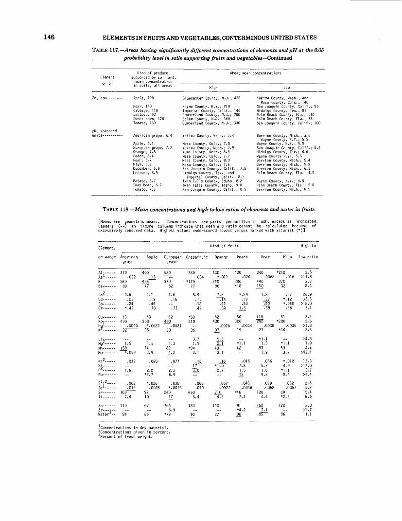
146 ELEMENTS IN FRUITS AND VEGETABLES, CONTERMINOUS UNITED STATES
TABLE 117.—Areas having significantly different concentrations of elements andpH at the 0.05 probability level in soils supporting fruits and vegetables—Continued
Element . or pH
pH, standard units----------
Kind of produce supported by soil and, mean concentration
in soils, all areas
Apple, 190
Pear, 140Cabbage, 110Lettuce, 53Sweet corn, 170Tomato, 150
American grape, 6.4
Apple, 6.4European grape, 7.2Orange, 7.8Peach, 6.4Pear, 6.7Plum, 6.7Cucumber, 6.9Lettuce, 6.9
Potato, 6.7Snap bean, 6.7Tomato, 7.3
Area; mean
High
Gloucester County, N.J.; 420
Wayne County, N.Y.; 210Imperial County, Calif.; 140Cumberland County, N.J.; 200Salem County, N.J. ; 360Cumberland County, N.J.; 330
Yakima County, Wash.; 7.4
Mesa County, Colo.; 7.8Yakima County, Wash.; 7.9Yuma County, Ariz. 8.8Mesa County, Colo. 7.7Mesa County, Colo. 8.0Mesa County, Colo. 7.6San Joaquin County Calif.; 7.5Hidalgo County, Tex. , and
Imperial County, Calif.; 8.1Twin Falls County, Idaho; 8.2Twin Falls County, Idaho; 8.0San Joaquin County, Calif.; 8.5
concentrations
Low
Yakima County, Wash., andMesa County, Colo.; 140
San Joaquin County, Calif.; 95Hidalgo County, Tex.; 81Palm Beach County, Fla.; <10Palm Beach County, Fla.; 78San Joaquin County, Calif.; 100
Berrien County, Mich., and Wayne County, N.Y.; 5.9
Wayne County, N.Y.; 5.5San Joaquin County, Calif.; 6.4Hidalgo County, Tex.; 6.6Wayne County N.Y.; 5.5Berrien County, Mich.; 5.4Berrien County, Mich.; 5.9Berrien County, Mich.; 6.3Palm Beach County, Fla.; 4.9
Wayne County, N.Y.; 4.8Palm Beach County, Fla., 5.8Berrien County, Mich.; 6.5
TABLE 118.—Mean concentrations and high-to-low ratios of elements and water in fruits
[Means are geometric means. Concentrations are parts per million in ash, except as indicated. Leaders (--) in figure columns indicate that mean and ratio cannot be calculated because of excessively censored data. Highest values underscored lowest values marked with asterisk (*)]
Element,
or water
i As 1———
D s
Co — —Cr— —
Cu — —iHg 1— -
Kz — —
Li—— —— Mg 2—— - Mn — — —
Na2 — —
P^ ......Pb ———
Si; 2-- Se 1 — - Sr — —
Zn ——— -Zr— =--Water-3-
Kind of fruit
American grape
370 .022
260 89
2.6 .23 .24
*.42
73 430
.004022
1.5 150
*.099
.039
1.6
.062
.012 160
7.4
110
84
Apple
400 .13 455 ——
~77
1.1 .19 .46 .70
63 350 *.0022
35
1.5 74 3.9
.060
2.2 *2.7
*.026 .0026
97 10
67
86
European grape
520
370 62
1.6.16
.73
62 490
.0031 20
1.3 62 4.2
.077
2.3 6.9
.038 *.0023
240
*66 6.9
*79
Grapefruit
.034 *170
77
5.9.16 .18 .47
*50 310
36
3.7 1.9
*34 3.1
.16
T70
.066
.010 650
5.4
130
IP-
Orange
430*.on260 86
7.8
!52 .80
52 430
.0026
5.3 77T 43 3.1
.16 *1.0 2.7
.067
.0077 710 ~472
140
87
Peach
430 .026
380 *18
*.29 .19 .30
1.3
56 300
.0034 19
42
.016 7.3 1.5I2
.043
.0046 *46
7.3
91 *4.2 90
Pear
340 .0068
440 150
1.8 .27 .90 769
110 290
.0038 23
l.*5 83 1.9
.056 5.7 1.6 9.8
.029
.0058 180
4.6
150
Plum
*210 .016
370 32
.57 *.12 *.050 .66
51 *200
.0035 *16
533.7
*.012 4.9
8.' 4
.032
.0057 89 *2.6
120
86
High-to-
low ratio
2.5
2.7 8.3
26.9 >2.3
>18.0 3.1
2.2 2.52.'3
>4.8 1.9 4.4
>42.4
13.3 >17.0
2.7 >4.4
2.6 5.2
15.4 6.5
2.3
l!l
^Concentrations in dry material. ^Concentrations given in percent. Percent of fresh weight.
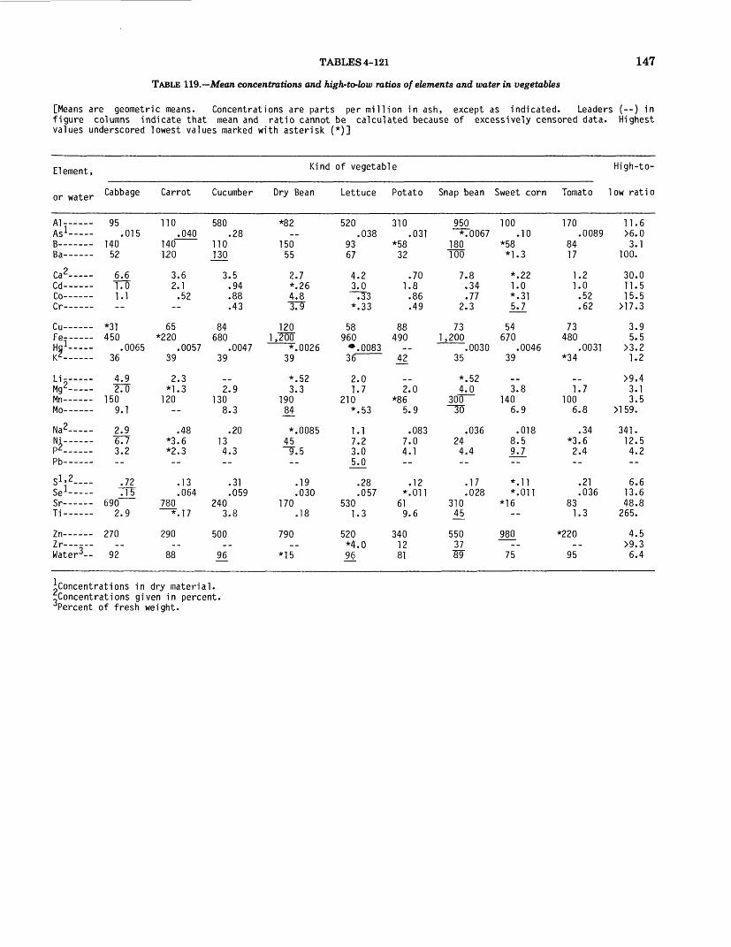
TABLES 4-121
TABLE 119.—Mean concentrations and high-to-low ratios of elements and water in vegetables
147
[Means are geometric means. Concentrations are parts per million in ash, except as indicated. Leaders (--) in figure columns indicate that mean and ratio cannot be calculated because of excessively censored data. Highest values underscored lowest values marked with asterisk (*)]
Element,
or water
A1_ _ _ _HI- ————— Ac-L _ __
R^-
Ta 2r* A
Co ———Cr ———
Cu ———FP- — --Ha 1
Kz
Li — —Mg^ ———Mn ————Mo ————
M-,2
Ni — —p2______Pb ———
S 1 ' 2— - Se 1— --cr___ _ _Ti ————
Zn ————Zr— -- WateH--
Cabbage
95 .015
140 52
6.6 1.0 1.1
*31 450
.0065 36
4.9 2.0
150 9.1
2.96.7 3.2
.72 7T5"
690 2.9
270
92
Carrot
110 .040
140 120
3.6 2.1 .52
65 *220
.0057 39
2.3 *1.3
120
.48 *3.6 *2.3
.13
.064 780
*.17
290
88
Cucumber
580 .28
110 130
3.5 .94 .88 .43
84 680
.0047 39
2.9130
8.3
.20 13 4.3
.31
.059 240
3.8
500
96^
Kind
Dry Bean
*82
150 55
2.7 *.26 4.8 1^
120 1,~2UO
*.0026 39
*.52 3.3
190 JJ4
*.0085 45 ~9.5
.19
.030 170
.18
790
*15
of vegetable
Lettuce
520 .038
93 67
4.2 3.0 ~^3 *.33
58 960 •.0083
2.0 1.7
210 *.53
1.1 7.2 3.0 5.0
.28
.057 530
1.3
520 *4.0 96
Potato
310 .031
*58 32
.70 1.8 .86 .49
88 490
ii2.0
*86 5.9
.083 7.0 4.1
.12*.on61 9.6
340 12 81
Snap bean
950 *.0067
180 100
7.8 .34 .77
2.3
73 1,200
.0030 35
*.52 4.0
300 ^0
.036 24 4.4
.17
.028 310 ^5
550 37 89
Sweet corn
100 .10
*58 *1.3
*.22 1.0 *.31 5.7
54 670
.0046 39
3.8 140
6.9
.018 8.5 9.7
*.ll*.on
*16
980
75
Tomato
170 .0089
84 17
1.2 1.0 .52 .62
73 480
.0031 *34
1.7 100
6.8
.34 *3.6 2.4
.21
.036 83 1.3
*220
95
High-to-
low ratio
11.6 >6.0 3.1
100.
30.0 11.5 15.5
>17.3
3.9 5.5
>3.2 1.2
>9.4 3.1 3.5
>159.
341. 12.5 4.2
6.6 13.6 48.8 265.
4.5 >9.3 6.4
^Concentrations in dry material. ^Concentrations given in percent. Percent of fresh weight.
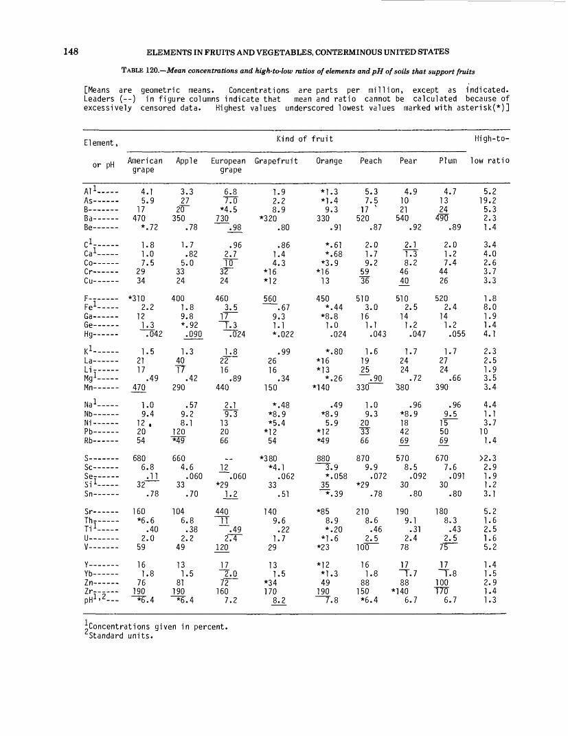
148 ELEMENTS IN FRUITS AND VEGETABLES, CONTERMINOUS UNITED STATES
TABLE 120.—Mean concentrations and high-to-low ratios of elements and pH of soils that support fruits
[Means are geometric means. Concentrations are parts per million, except as indicated.Leaders (—) in figure columns indicate that mean and ratio cannot be calculated because ofexcessively censored data. Highest values underscored lowest values marked with asterisk(*)]
Element,
or pH
Al 1 -Ac-- __ __
R__.____D ,
Be ———
C 1— —Ca 1Co ————r>------Cu- ———
FF;r::::Ga ———Ge- ———Hg— —
K 1 -
M_ _ _ _1 Mg 1 ———
Mn ————
Na 1 ———Nb — —Ni ———Pb— —Dk
$--_ _ _Sc ___ -*J\*
Se- _ --i c-i 1 _ __Sn ———
$r-__ _Thr~—Ti 1— --U ————V-— —
Y — - —vh---- _Zn ——— -Zr ———pH 1 ' 2—
Kind of fruit
American grape
4.1 5.9
17 470 *.72
1.8 1.0 7.5
29 34
*310 2.2
12 1.3 .042
1.5 21 17
.49 470
1.0 9.4
12 . 20 54
680 6.8 .11
32 .78
160 *6.6
.40 2.0
59
16 1.8
76 190 ~*6.4
Apple
3.3 27
20 350
.78
1.7 .82
5.0 33 24
400 1.8 9.8 *.92 .090
1.3 40 T7
.42 290
.57 9.2 8.1
120 *49
660 4.6 .060
33 .70
104 6.8 .38
2.2 49
13 1.5
81 190 *6.4
European grape
6.8 770 *4.5
730 .98
.96 2.7 10 3T 24
460 3.5 1T~
T.3 .024
1.8 22 16
.89 440
2.1 "O
13 20 66
12 .060
*29 1.2
440 11
.49 2JT
120
17 2.0
72 160
7.2
Grapefruit
1.9 2.2 8.9
*320 .80
.86 1.4 4.3
*16 *12
560 —— .67
9.3 1.1 *.022
.99 26 16
.34 150
*.48 *8.9 *5.4
*12 54
*380 *4.1
.062 33
.51
140 9.6 .22
1.7 29
13 1.5
*34 170
8.2
Orange
*1.3 *1.4 9.3
330 .91
*.61 *.68
*3.9 *16 13
450 *.44
*8.8 1.0 .024
*.80 *16 *13
*.26 *140
.49 *8.9 5.9
*12 *49
8803.9 *.058
35 *.39
*85 8.9 *.20 *1.6
*23
*12 *1.3 49
190 ~~7.8
Peach
5.3 7.5 17 x
520 .87
2.0 1.7 9.2
59 36
510 3.0
16 1.1 .043
1.6 19 25 ~.90 330
1.0 9.3
20 31 66
870 9.9 .072
*29 .78
210 8.6 .46
2.5 100
16 1.8
88 150 *6.4
Pear
4.9 10 21 540
.92
2.11.3 8.2
46 _40
510 2.5
14 1.2 .047
1.7 24 24
.72 '380
.96 *8.9 18 42 6£
570 8.5 .092
30 .80
190 9.1 .31
2.4 78
17 ~T.7 88
*140 6.7
Plum
4.7 13 24
4~90 .89
2.0 1.2 7.4
44 26
520 2.4
14 1.2 .055
1.7 27 24
.66 390
.96 9.5
15 50 69.
670 7.6 .091
30 .80
180 8.3 .43
2.5 75
17 ~T.8 100 T70
6.7
High-to-
low ratio
5.2 19.2 5.3 2.3 1.4
3.4 4.0 2.6 3.7 3.3
1.8 8.0 1.9 1.4 4.1
2.3 2.5 1.9 3.5 3.4
4.4 1.1 3.7
10 1.4
>2.3 2.9 1.9 1.2 3.1
5.2 1.6 2.5 1.6 5.2
1.4 1.5 2.9 1.4 1.3
^Concentrations given in percent.
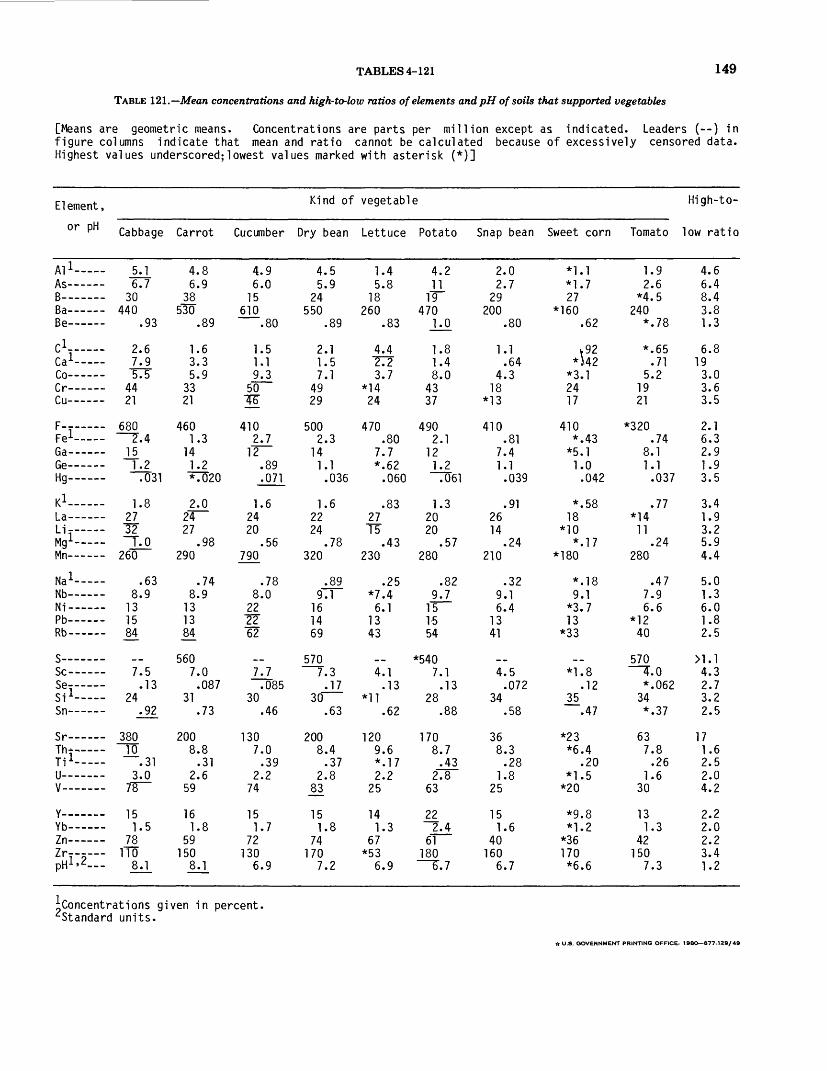
TABLES 4-121 149
TABLE 121.— Mean concentrations and high-to-low ratios of elements andpH of soils that supported vegetables
[Means are geometric means. Concentrations are parts per million except as indicated. Leaders (--) in figure columns indicate that mean and ratio cannot be calculated because of excessively censored data. Highest values underscored;lowest values marked with asterisk (*)]
Element, or pH
Al 1— -
Be ———
C 1Ca 1 -- -Co— — -
Cu ———
lli:::::Ga— —Ge ———Hg ———
K 1La — —LiMg 1 ———Mn ———
Ma !---_-Nb ———Ni ———Pb ———Rb ———
S ————Sr- _ - _SP-- __ -1 Si 1——Sn ———
Thr— - T1 1—— -U ————V ————
Y ————WL
Zn ———Zr ———pHl.2—
Cabbage
5.1 6.7
30 440
.93
2.6 7.9 5.5
44 21
680 ~T.4 15 1.2 .031
1.8 27 12 ~T.O 260
.63 8.9 13 15 _84
7.5 .13
24 .92
380 H
3.0
15 1.5
78 110
8.1
Carrot
4.8 6.9
38 530
.89
1.6 3.3 5.9
33 21
460 1.3
14 1.2 *.020
2.0
27 .98
290
.74 8.9 13 13 _84
560 7.0 .087
31 .73
200 8.8 .31
2.6 59
16 1.8
59 150
8.1
Cucumber
4.9 6.0
15 610
.80
1.5 1.1 9.3
50 JG
410 2.7
12 .89 .071
1.6 24 20
.56 790
.78 8.0
22 22 •62
7.7 .085
30 .46
130 7.0 .39
2.2 74
15 1.7
72 130
6.9
Kind of
Dry bean
4.5 5.9
24 550
.89
2.1 1.5 7.1
49 29
500 2.3
14 1.1 .036
1.6 22 24
.78 320
.89 9.1
16 14 69
570 ~~7.3
.17 30 ——
.63
200 8.4 .37
2.8 _83
15 1.8
74 170
7.2
vegetable
Lettuce
1.4 5.8
18 260
.83
4.4 "272 3.7
*14 24
470 .80
7.7 *.62 .060
.83 _27
.43 230
.25 *7.4 6.1
13 43
4.1 .13
.62
120 9.6 *.17 2.2
25
14 1.3
67 *53
6.9
Potato
4.2 11
19 470
1.0
1.8 1.4 8.0
43 37
490 2.1
12 1.2 .061
1.3 20 20
.57 280
.82 9.7 15 15 54
*540 7.1 .13
28 .88
170 8.7 .43 2T8~
63
22
61 180
Snap bean
2.0 2.7
29 200
.80
1.1 .64
4.3 18
*13
410 .81
7.4 1.1 .039
.91 26 14
.24 210
.32 9.1 6.4
13 41
4.5 .072
34 .58
36 8.3 .28
1.8 25
15 1.6
40 160
6.7
Sweet corn
*1.7 27
*160 .62
v92 *)42
*3.1 24 17
410 *.43
*5.1 1.0 .042
*.58 18
*10 *.17
*180
*.18 9.1 *3.7 13
*33
*1.8 .12
35 .47
*23 *6.4
.20 *1.5 *20
*9.8 *1.2
*36 170 *6.6
Tomato
1.9 2.6
*4.5 240
*.78
*.65 .71
5.2 19 21
*320 .74
8.1 1.1 .037
.77 *14 11
.24 280
.47 7.9 6.6
*12 40
570
*.062 34 *.37
63 7.8 .26
1.6 30
13 1.3
42 150
7.3
High-to-
low ratio
4.6 6.4 8.4 3.8 1.3
6.8 19 3.0 3.6 3.5
2.1 6.3 2.9 1.9 3.5
3.4 1.9 3.2 5.9 4.4
5.0 1.3 6.0 1.8 2.5
4^3 2.7 3.2 2.5
17 1.6 2.5 2.0 4.2
2.2 2.0 2.2 3.4 1.2
^Concentrations given in percent.-Standard units.
ft U.S. GOVERNMENT PRINTING OFFICE: 198O—677.129/49