1

Elementary Statistical Methods

André L. Souza, Ph.D.The University of Alabamawww.andreluizsouza.com

Lecture 24One-way Analysis of Variance

2

The basic idea

• So far, we have been comparing two sampleso boys vs. girlso drinkers vs. non-drinkerso beautiful vs. ugly

• What if we want to compare more than two samples?o For example: Supposed I want to investigate whether study time influences

student’s grades. In other words, I want to know if studying two hours vs. four hours vs. six hours significantly change students’ grades.

• One way to investigate this would be to conduct three separate experiments.o Two hours vs. four hourso Two hours vs. six hourso Four hours vs. six hours

• Why is that not a good idea?

3

The basic idea

• A better way to investigate my hypothesis is to perform one single experiment that tests all three groups at the same time

• Why not carry separate t-tests for each pairwise comparison?o The more groups you have, the more t-tests you will needo Each t-test is associated with an α–level (probability of making a Type I error)o Multiple t-tests will increase the overall probability of Type I error

• A common method used to compare several means while keeping the Type I error rate small is known as Analysis of Variance

• ANOVA is a statistical technique for testing/comparing differences in the means of several groups

4

Analysis of Variance

• Analysis of Variance is probably the most used statistical technique in psychological research

• If the analysis of variance uses only one independent variable (i.e., just one explanatory variable), it is known as one-way Analysis of Variance (or One-Way ANOVA)o Influence of hours of study (independent variable) on student’s grades

(dependent variable)o Influence of types of beer (independent variable) on people’s perceptions of

beauty (dependent variable)o Influence of a person’s origin (independent variable) on his/her mate

preferences (dependent variable)

• The groups that make up the independent variable are known as levels of that variableo Hours of study (two, four and six)o Types of beer (Budweiser, Corona, Heineken)o Person’s origin (Alabama, Texas, Michigan)

5

Analysis of Variance

• Analysis of Variance will focus on the variance of each sample• Variance indicates how far a set of number is spread out• Variance is the standard deviation squared

• The fundamental strategy in ANOVA is: we will take the total variance of all the scores and split it into two parts: variance caused by the independent variable and variance caused by chance (error variance).

• We then form a ratio between these two variances. If this ratio is significantly bigger than one, then the variation due to the independent variable is significantly higher

Variance Partitioning

Total Variability

Variability caused by

IV

Variability due to chance

7

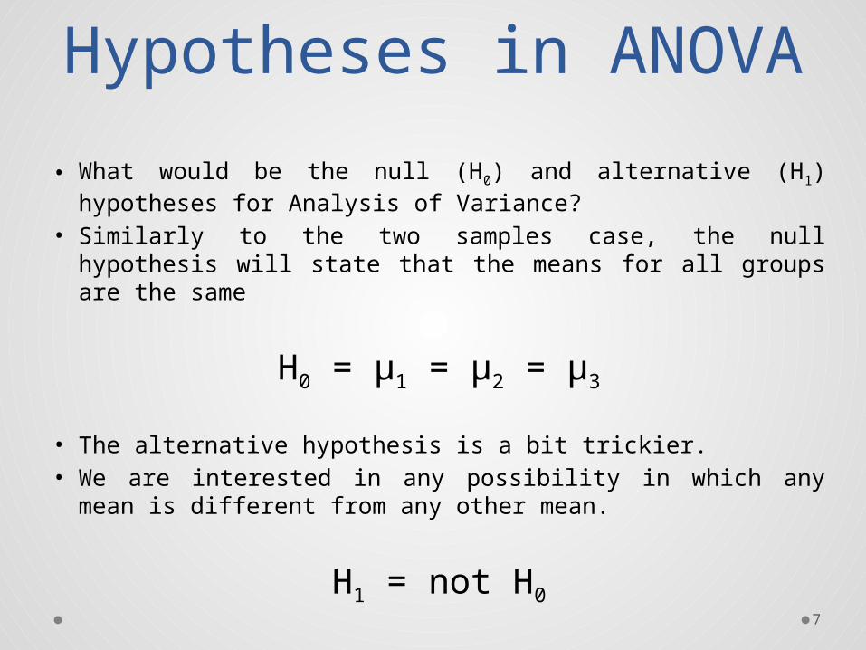
Hypotheses in ANOVA

• What would be the null (H0) and alternative (H1) hypotheses for Analysis of Variance?

• Similarly to the two samples case, the null hypothesis will state that the means for all groups are the same

H0 = μ1 = μ2 = μ3

• The alternative hypothesis is a bit trickier.• We are interested in any possibility in which any mean

is different from any other mean.

H1 = not H0

8

Hours of Study Example

Two Hours Four Hours Six Hours

60 71 83

58 77 79

57 73 85

61 69 90

68 75 93

• How many means can you calculate from this dataset?o The mean grade for the two-hours groupo The mean grade for the four-hours groupo The mean grade for the six-hour groupo And a new mean called the Grand Mean, which is the mean of all the

numbers together

9

Sum of Squares

• In Analysis of Variance, we measure total variability using Sum of Squares

• SS is the sum of all the squared deviations from the mean

• In One-way ANOVA there are three different types of Sum of Squareso Total Sum of Squares (SST)

o Treatment Sum of Squares (SSA)

o Error Sum of Squares (SSE)

10

Total Sum of Squares• This represents the total variability regardless of any

specific treatment• In the hours of study example, the SST is the amount

that the grades vary regardless of how many hours the person studied

• You take each grade, subtract from it the Grand Mean, square the result and add them all up

Two Hour

s

Four Hour

s

Six Hour

s

60 71 83

58 77 79

57 73 85

61 69 90

68 75 93

GM = 73.26

SST = (60 - 73.26)2 + (58 – 73.26)2 + … + (93 – 73.26)2

SST = 1826.93

11

Treatment Sum of Squares

• This represents the variability between treatment means• Each group has its own mean. And this mean is far from

the grand mean by a certain amount• SSA measures this variability

• You replace each score by its respective mean, subtract from it the Grand Mean, square the result and add them all up

Two Hour

s

Four Hour

s

Six Hour

s

60 71 83

58 77 79

57 73 85

61 69 90

68 75 93

12

Treatment Sum of Squares

• This represents the variability between treatment means• Each group has its own mean. And this mean is far from

the grand mean by a certain amount• SSA measures this variability

• You replace each score by its respective mean, subtract from it the Grand Mean, square the result and add them all up

Two Hour

s

Four Hour

s

Six Hour

s

60.8 73 86

60.8 73 86

60.8 73 86

60.8 73 86

60.8 73 86

GM = 73.26

SSA = (60.8 - 73.26)2 + (60.8 – 73.26)2 +(73 – 73.26)2 + … + (86 – 73.26)2

SSA = 1584.38

13

Error Sum of Squares• This represents the variability within each treatment mean• Each group has its own mean. Each score in that groups

deviates from its specific mean by a certain amount• SSE measures this variability

• You take each score, subtract from it the mean of its group, square the result and add them all up. Then add the individual SS of each group

Mean for Two-hours group = 60.8Mean for Four-hours group = 73Mean for Six-hours group = 86

SSE = (60.8 – 60.8)2 + (71 – 73)2 + … + (83 – 86)2

SSE = 242.55

Two Hour

s

Four Hour

s

Six Hour

s

60 71 83

58 77 79

57 73 85

61 69 90

68 75 93

14

Variance (SS) partitioning

• You should have noticed that the SSA + SSE = SST

• This means that the Total Variability can be partitioned into variability that can be attributed to the treatment group (i.e., whatever makes the groups different) and variability that cannot be attributed to treatment groups (variability due to chance)

• Now, think about the null hypothesis for a second. If there is no difference between the groups, we should expect the variability within each group to be the same across (between) groups

• But because this two variabilites (between and within) are not “equally” represented, we need to take the average of them

15

Mean Squares• To obtain the average deviation, we divide the SS by degrees of

freedom to obtain what we call mean square

• The SSA is represented by the number of groups in the experiment

• Then to average the SSA, we need to divide the SSA by the degrees of freedom related to the number of groups (number of groups – 1)

• The SSE is represented by the number of people in each group

• Then, to average the SSE, we need to divide the SSE by the degrees of freedom related to the number of people in each group (number of people in each group -1 times the number of groups)

16

MSA and MSE ratio

• Remember that MSE represents the average variation within each group.

• If the groups are the same, we expect this variation to be the same for all groups

• Then we expect the variation between groups to be the same as the variation between groups (MSA)

Two Hour

s

Four Hour

s

Six Hour

s

60 60 60

60 60 60

60 60 60

60 60 60

60 60 60

• If MSA and MSE are the same, we expect the ratio MSA/MSE to be 1

• If MSA is larger than MSE, then we expect the ratio MSA/MSE to be larger than 1

• If MSA is smaller than MSE, then we expect the ratio MSA/MSE to be smaller than 1

17

Analysis of Variance

• Statistical technique utilized to look for differences between more than two groups

• It splits the total variability in the dataset into two partso Variability caused by treatmentso Variability caused by chance

• If there is no difference between the groups, these two amounts of variability should be the same

• This is the logic behind Analysis of Variance

18

ANOVA TableSource SS df MS F

Treatment

Error

Total

• The ANOVA table is a summary of the SS and MS for a given experiment

• The equality of the variances is tested in terms of the ratio between MSA and MSE

• This ratio (ratio between variances) is represented in terms of F

19

F-statistic

• The F-statistic is obtained by dividing MSA by MSE

• In Analysis of Variance, we reject H0 only if the computed value of F is significantly greater than 1

• How much larger than 1 the value for the F needs to be before we decide to reject H0?

• If H0 is true, F is distributed as the F distribution

• It will have dfA and dfE degrees of freedom

• Similarly to what we have done to find t-critical, to find the F-critical, we need to look up this value at the F-table

• If the F-statistic is larger than the F-critical, then we reject H0 that states that all the means are the same

20

F-Table

21

Example• I suspect that the brand of cellphone you have

affects the amount of texts you send per day• To test this, I have randomly selected

o 5 users of Galaxy S5o 5 users of Nexus 6o 5 users of iPhone 6

ExampleGalaxy S5 Nexus 6 iPhone 6

10 94 33

12 44 21

15 34 23

23 69 18

32 77 10

• If the cellphone model does not affect the number of texts a person sends a day, then we would expect:

• H0 = μGalaxy = μNexus = μiPhone

• If the cellphone model does influence then:• H1 = not H0

23

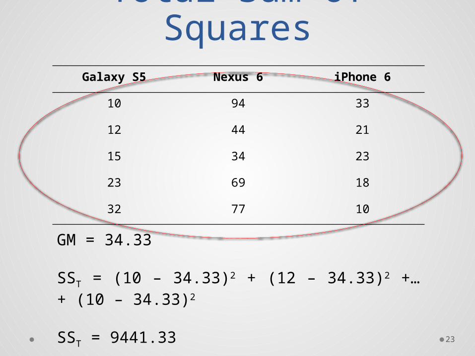
Total Sum of SquaresGalaxy S5 Nexus 6 iPhone 6

10 94 33

12 44 21

15 34 23

23 69 18

32 77 10

GM = 34.33

SST = (10 – 34.33)2 + (12 – 34.33)2 +… + (10 – 34.33)2

SST = 9441.33

24

Treatment Sum of Squares

Galaxy S5 Nexus 6 iPhone 6

10 94 33

12 44 21

15 34 23

23 69 18

32 77 10

25

Treatment Sum of Squares

Galaxy S5 Nexus 6 iPhone 6

18.4 63.6 21

18.4 63.6 21

18.4 63.6 21

18.4 63.6 21

18.4 63.6 21

GM = 34.33

SSA = (18.4 – 34.33)2 + (63.6 – 34.33)2 +… + (21 – 34.33)2

SSA = 6440.9

26

Error Sum of SquaresGalaxy S5 Nexus 6 iPhone 6

10 94 33

12 44 21

15 34 23

23 69 18

32 77 10

Galaxy = 18.4Nexus = 63.9iPhone = 21

SSE = (10 – 18.4)2 + (94 – 63.6)2 +… + (33 – 21)2 SSE = 3000.4

27

ANOVA TableSource SS df MS F

Cell Phone

6440.9 2 3220.5 12.88

Error 3000.4 12 250.03

Total 9441.3 14

• The F-critical for this test is F(2,12) = 3.89 (α = 0.05)• If the F-statistic is larger than the F-critical, then we reject

H0 = μGalaxy = μNexus = μiPhone

• If the F-statistic is not larger than F-critical, we fail to reject H0

• Because 12.88 is larger than 3.89, we reject H0 and conclude that cellphone model does influence the amount of texts people send per day

28

Elementary Statistical Methods

André L. Souza, Ph.D.The University of Alabamawww.andreluizsouza.com

Lecture 24

Thank you!