ELEMENTARY NUMBER THEORY - Tel Aviv Universityjarden/Courses/numb.pdf · ELEMENTARY NUMBER THEORY...

ELEMENTARY NUMBER THEORY

Notes by

Moshe Jarden

School of Mathematics, Tel Aviv University

Ramat Aviv, Tel Aviv 69978, Israel

e-mail: [email protected]

web page: http://www.tau.ac.il/∼jarden/Courses

Forward

We start with the set of natural numbers, N = {1, 2, 3, . . .} equipped with the familiar addition

and multiplication and assume that it satisfies the induction axiom. It allows us to establish

division with a residue and the Euclid’s algorithm that computes the greatest commond divisor

of two natural numbers. It also leads to a proof of the fundamental theorem of arithmetic:

Every natural number is a product of prime numbers in a unique way up to the order of the

factors. Euclid’s theorem about the infinitude of the prime numbers is a consequence of that

theorem.

Next we introduce congruences and the Euler’s ϕ-function (ϕ(n) is the number of the

natural numbers between 1 and n that are relatively prime to n). Then we prove Euler’s

theorem: aϕ(n) ≡ 1 mod n for each natural number n and every integer a relatively prime to

n. We also prove the Chinese remainder theorem and conclude the multiplicity of the Euler

phi function: ϕ(mn) = ϕ(m)ϕ(n) if m and n are relatively prime. This theorem is the main

ingredient in the first and most applied public key in cryptography. Next we prove that each

prime number p has ϕ(p− 1) primitive roots modulo prime numbers.

Most of this material enters into the proof of the quadratic reciprocity law: Every distinct

odd prime numbers p, q satisfy(

qp

)= (−1)

p−12

q−12

(pq

), where

(qp

)= 1 if there exists an integer

x with x2 ≡ q mod p, and −1 otherwise.

The last part of these notes is devoted to the proof of Dirichlet’s theorem about the

Dirichlet density of the set prime numbers p ≡ a mod m, where gcd(a, m) = 1.

Mevasseret Zion, 4 April 2012

Table of Contents

1. Natural Numbers . . . . . . . . . . . . . . . . . . . . . . . . . . . . 1

2. Division with a Residue . . . . . . . . . . . . . . . . . . . . . . . . . 4

3. Greatest Common Divisor . . . . . . . . . . . . . . . . . . . . . . . . 7

4. The Prime Numbers . . . . . . . . . . . . . . . . . . . . . . . . . 12

5. The p-adic Valuation . . . . . . . . . . . . . . . . . . . . . . . . . 15

6. Infinitude of Prime Numbers . . . . . . . . . . . . . . . . . . . . . . 18

7. Congruences . . . . . . . . . . . . . . . . . . . . . . . . . . . . . 20

8. The Ring Z/nZ . . . . . . . . . . . . . . . . . . . . . . . . . . . 23

9. Fermat’s Little Theorem . . . . . . . . . . . . . . . . . . . . . . . . 26

10. Polynomials . . . . . . . . . . . . . . . . . . . . . . . . . . . . 30

11. Wilson’s Theorem . . . . . . . . . . . . . . . . . . . . . . . . . . 33

12. Density of Prime Numbers . . . . . . . . . . . . . . . . . . . . . . 35

13. Chinese Remainder Theorem . . . . . . . . . . . . . . . . . . . . . 37

14. Euler’s Phi Function and Cryptography . . . . . . . . . . . . . . . . 35

15. Primitive Roots . . . . . . . . . . . . . . . . . . . . . . . . . . . 44

16. Quadratic Equations Modulo p . . . . . . . . . . . . . . . . . . . . 46

17. Legendre Symbol . . . . . . . . . . . . . . . . . . . . . . . . . . 48

18. More on Polynomials . . . . . . . . . . . . . . . . . . . . . . . . . 51

19. The Binomial Formula . . . . . . . . . . . . . . . . . . . . . . . . 55

20. The Quadratic Reciprocity Law . . . . . . . . . . . . . . . . . . . . 59

21. The Jacobi Symbol . . . . . . . . . . . . . . . . . . . . . . . . . 61

22. Characters of Finite Abelian Groups . . . . . . . . . . . . . . . . . . 64

23. Dirichlet’s Series . . . . . . . . . . . . . . . . . . . . . . . . . . 68

24. Riemann Zeta Function . . . . . . . . . . . . . . . . . . . . . . . 72

25. Characters Modulo m . . . . . . . . . . . . . . . . . . . . . . . . 74

26. Euler Products . . . . . . . . . . . . . . . . . . . . . . . . . . . 76

27. Abscissa of Convergence . . . . . . . . . . . . . . . . . . . . . . . 79

28. Non-Vanishing of L(1, χ) . . . . . . . . . . . . . . . . . . . . . . . 81

29. Proof of Dirichlet’s Theorem . . . . . . . . . . . . . . . . . . . . . 84

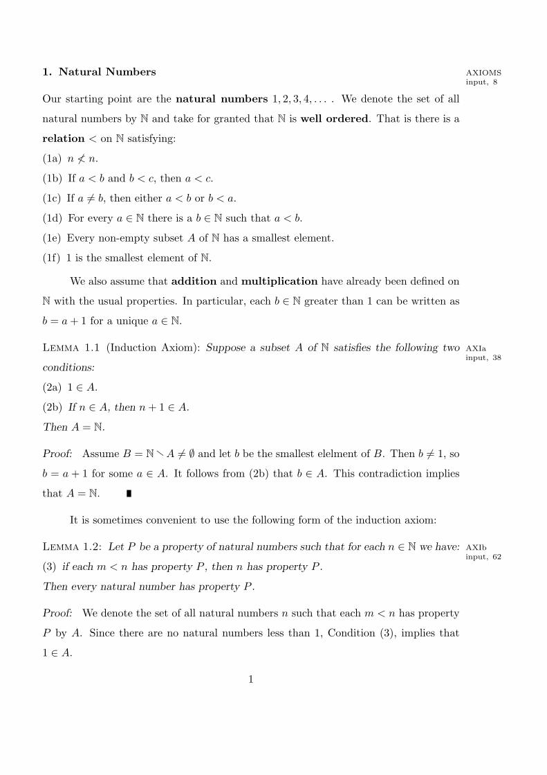
1. Natural Numbers AXIOMSinput, 8

Our starting point are the natural numbers 1, 2, 3, 4, . . . . We denote the set of all

natural numbers by N and take for granted that N is well ordered. That is there is a

relation < on N satisfying:

(1a) n 6< n.

(1b) If a < b and b < c, then a < c.

(1c) If a 6= b, then either a < b or b < a.

(1d) For every a ∈ N there is a b ∈ N such that a < b.

(1e) Every non-empty subset A of N has a smallest element.

(1f) 1 is the smallest element of N.

We also assume that addition and multiplication have already been defined on

N with the usual properties. In particular, each b ∈ N greater than 1 can be written as

b = a + 1 for a unique a ∈ N.

Lemma 1.1 (Induction Axiom): Suppose a subset A of N satisfies the following two AXIainput, 38

conditions:

(2a) 1 ∈ A.

(2b) If n ∈ A, then n + 1 ∈ A.

Then A = N.

Proof: Assume B = NrA 6= ∅ and let b be the smallest elelment of B. Then b 6= 1, so

b = a + 1 for some a ∈ A. It follows from (2b) that b ∈ A. This contradiction implies

that A = N.

It is sometimes convenient to use the following form of the induction axiom:

Lemma 1.2: Let P be a property of natural numbers such that for each n ∈ N we have: AXIbinput, 62

(3) if each m < n has property P , then n has property P .

Then every natural number has property P .

Proof: We denote the set of all natural numbers n such that each m < n has property

P by A. Since there are no natural numbers less than 1, Condition (3), implies that

1 ∈ A.

1

Now suppose that n ∈ A. Then each m < n has property P . By (3), n has

property P , so all m < n + 1 has property P . By definition, n + 1 ∈ A. It follows from

the induction axiom that A = N. Since each n ∈ N satisfies n < n + 1 and n + 1 ∈ A,

we get that n has property P .

If a < b, then there exists a unique x ∈ N such that a+x = b. As usuall, we write

x = b− a. If b ≤ a, then b− a is not defined within N. So, we consider also the number

0 and the negative number −n for each n ∈ N and extend addition and multiplication

to the set Z = {0,±1,±2,±3, . . .} of integers. Then Z is a commutative ring with

1, that is it satisfies the following conditions for all x, y, z ∈ Z:

(4a) x + y = y + x (commutative law for addition).

(4b) (x + y) + z = x + (y + z) (associative law of addition).

(4c) 0 + x = x.

(4d) For each a ∈ Z there exists a unique element −a ∈ Z such that a + (−a) = 0.

(5a) xy = yx (commutative law of multiplication).

(5b) (xy)z = x(yz) (associative law of multiplication).

(5c) 1 · x = x.

(6) x(y + z) = xy + xz (distributive law).

It is also convenient to consider also the field Q of all quotients ab with a, b ∈ Z

and b 6= 0. It satisfies Conditions (4), (5), and (6), for all x, y, z ∈ Q and in addtion

also the following one:

(5d) For each x 6= 0 there exists a unique element x−1 ∈ Q such that x · x−1 = 1.

Exercise 1.3: Prove that N is an infinite set, that is there exist no n ∈ N and a AXIcinput, 127

bijective function f : N → {1, . . . , n}. Hint: You are allowed to use the following set

theoretic rule: Every injective map f from a finite set A onto itself is bijective. Then

apply this rule to A = {1, . . . , n} and observe that n + 1 /∈ {1, . . . , n}.

Exercise 1.4: Use induction on n (or otherwise) to prove the following formulas: AXIdinput, 139

n∑

k=1

k =n(n + 1)

2(7a)

2

n∑

k=1

k2 =n(n + 1)(2n + 1)

6(7b)

n∑

k=1

k3 =n2(n + 1)2

4(7c)

Exercise 1.5: Prove that every real number x 6= 1 satisfies∑n

i=0 xi = xn+1−1x−1 . AXIe

input, 155

Exercise 1.6: Define F0 = 0, F1 = 1, and assuming that Fn and Fn+1 have beed AXIfinput, 160

defined, let Fn+2 = Fn+1 + Fn. One calls F0, F1, F2, . . . the Fibonacci numbers.

Prove by induction on n that Fn <(74

)n. Hint: Use that 44 < 49.

Exercise 1.7: Let A be a nonempty subset of Z. Suppose that A is bounded from AXIg

input, 168above. That is, there exist r ∈ Q such that a ≤ r for all a ∈ A. Prove that A has a

maximal element. Hint: Let b the largest integer k satisfying b ≤ r (one denotes that

number by [r]). Then consider the set A′ = {b− a | a ∈ A}.

3

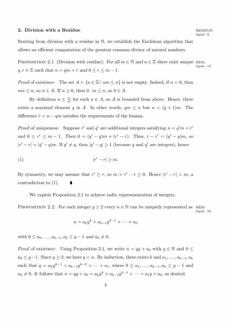
2. Division with a Residue RESIDUEinput, 6

Starting from division with a residue in N, we establish the Euclidean algorithm that

allows an efficient computation of the greatest common divisor of natural numbers.

Proposition 2.1 (Division with residue): For all m ∈ N and n ∈ Z there exist unique RESainput, 13

q, r ∈ Z such that n = qm + r and 0 ≤ r ≤ m− 1.

Proof of existence: The set A = {a ∈ Z | am ≤ n} is not empty. Indeed, if n < 0, then

nm ≤ n, so n ∈ A. If n ≥ 0, then 0 ·m ≤ n, so 0 ∈ A.

By definition a ≤ nm for each a ∈ A, so A is bounded from above. Hence, there

exists a maximal element q in A. In other words, qm ≤ n but n < (q + 1)m. The

difference r = n− qm satisfies the requirements of the lemma.

Proof of uniqueness: Suppose r′ and q′ are additional integers satisfying n = q′m + r′

and 0 ≤ r′ ≤ m − 1. Then 0 = (q′ − q)m + (r′ − r). Thus, r − r′ = (q′ − q)m, so

|r′ − r| = |q′ − q|m. If q′ 6= q, then |q′ − q| ≥ 1 (because q and q′ are integers), hence

(1) |r′ − r| ≥ m.

By symmetry, we may assume that r′ ≥ r, so m > r′ − r ≥ 0. Hence |r′ − r| < m, a

contradiction to (1).

We exploit Proposition 2.1 to achieve radix represenentation of integers.

Proposition 2.2: For each integer g ≥ 2 every n ∈ N can be uniquely represented as RESbinput, 54

n = akgk + ak−1gk−1 + · · ·+ a0

with 0 ≤ a0, . . . , ak−1, ak ≤ g − 1 and ak 6= 0.

Proof of existence: Using Proposition 2.1, we write n = qg + a0 with q ∈ N and 0 ≤a0 ≤ g−1. Since g ≥ 2, we have q < n. By induction, there exists k and a1, . . . , ak−1, ak

such that q = akgk−1 + ak−1gk−2 + · · · + a1, where 0 ≤ a1, . . . , ak−1, ak ≤ g − 1 and

ak 6= 0. It follows that n = qg + a0 = akgk + ak−1gk−1 + · · ·+ a1g + a0, as desired.

4

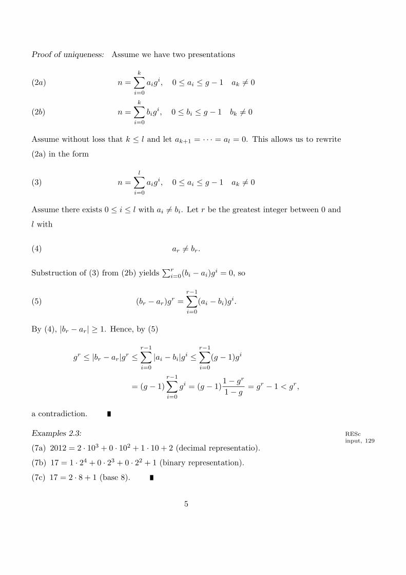
Proof of uniqueness: Assume we have two presentations

n =k∑

i=0

aigi, 0 ≤ ai ≤ g − 1 ak 6= 0(2a)

n =k∑

i=0

bigi, 0 ≤ bi ≤ g − 1 bk 6= 0(2b)

Assume without loss that k ≤ l and let ak+1 = · · · = al = 0. This allows us to rewrite

(2a) in the form

(3) n =l∑

i=0

aigi, 0 ≤ ai ≤ g − 1 ak 6= 0

Assume there exists 0 ≤ i ≤ l with ai 6= bi. Let r be the greatest integer between 0 and

l with

(4) ar 6= br.

Substruction of (3) from (2b) yields∑r

i=0(bi − ai)gi = 0, so

(5) (br − ar)gr =r−1∑

i=0

(ai − bi)gi.

By (4), |br − ar| ≥ 1. Hence, by (5)

gr ≤ |br − ar|gr ≤r−1∑

i=0

|ai − bi|gi ≤r−1∑

i=0

(g − 1)gi

= (g − 1)r−1∑

i=0

gi = (g − 1)1− gr

1− g= gr − 1 < gr,

a contradiction.

Examples 2.3: REScinput, 129

(7a) 2012 = 2 · 103 + 0 · 102 + 1 · 10 + 2 (decimal representatio).

(7b) 17 = 1 · 24 + 0 · 23 + 0 · 22 + 1 (binary representation).

(7c) 17 = 2 · 8 + 1 (base 8).

5

Exercise 2.4: The greengrocer Reuven has a scale and for each integer n ≥ 0 he has RESdinput, 139

one weight weighing 2n kilos. Explain how can Reuven weigh each merchandise weighing

a positive integral number of kilos.

Exercise 2.5: Also the butcher Shimeon has a scale and for each n ≥ 0 he has one RESeinput, 146

weight weighing 3n kilos. Explain how can Shimeon weigh each merachndise weighing

a positive integral number of kilos.

6

hypothesis yields a common divisor d of r and a. By (3), d is also the greatest common

divisor of a and b.

Following Proposition 3.2, we write gcd(a, b) for the unique greatest common

divisor of a and b. It turns out that gcd(a, b) is a linear combination of a and b with

integral coefficients:

Proposition 3.3: For all a, b ∈ N there exist x, y ∈ Z such that gcd(a, b) = ax + by. DIVcinput, 86

Proof: We proceed again by induction on min(a, b). Without loss we assume that

a ≤ b and divide b by a as in (3). If r = 0, then a = gcd(a, b) = 1 · a + 0 · b. Otherwise

d = gcd(a, b) = gcd(a, r) and min(a, r) = r < a = min(a, b). The induction hypothesis

gives x′, y′ ∈ Z such that d = ax′ + ry′. Substitution r from (3) in the latter equality,

we get

d = ax′ + (b− qa)y′ = ax′ + by′ − qay′ = a(x′ − qy′) + by′,

as desired.

The usual algorithm to compute the greatest common divisor of natural numbers

uses factorization of those numbers into products of prime numbers. If the numbers

involved are big, the factorization is a lengthy operation. We propose a much quicker

procedure:

Procedure 3.4: The Euclid algorithm for the computation of the greatest common di- DIVdinput, 118

visor. Given natural numbers a ≤ b we apply division with residue several times to

compute a descending sequence of natural numbers a = r0 > r1 > · · · > rn > 0 and a

8

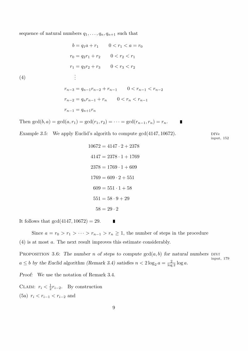
sequence of natural numbers q1, . . . , qn, qn+1 such that

(4)

b = q1a + r1 0 < r1 < a = r0

r0 = q2r1 + r2 0 < r2 < r1

r1 = q3r2 + r3 0 < r3 < r2

...

rn−3 = qn−1rn−2 + rn−1 0 < rn−1 < rn−2

rn−2 = qnrn−1 + rn 0 < rn < rn−1

rn−1 = qn+1rn

Then gcd(b, a) = gcd(a, r1) = gcd(r1, r2) = · · · = gcd(rn−1, rn) = rn.

Example 3.5: We apply Euclid’s algorith to compute gcd(4147, 10672). DIVeinput, 152

10672 = 4147 · 2 + 2378

4147 = 2378 · 1 + 1769

2378 = 1769 · 1 + 609

1769 = 609 · 2 + 551

609 = 551 · 1 + 58

551 = 58 · 9 + 29

58 = 29 · 2

It follows that gcd(4147, 10672) = 29.

Since a = r0 > r1 > · · · > rn−1 > rn ≥ 1, the number of steps in the procedure

(4) is at most a. The next result improves this estimate considerably.

Proposition 3.6: The number n of steps to compute gcd(a, b) for natural numbers DIVfinput, 179

a ≤ b by the Euclid algorithm (Remark 3.4) satisfies n < 2 log2 a = 2log 2 log a.

Proof: We use the notation of Remark 3.4.

Claim: ri < 12ri−2. By construction

(5a) ri < ri−1 < ri−2 and

9

(5b) ri−2 = qiri−1 + ri.

If ri−1 ≤ 12ri−2, then ri < 1

2ri−2 (by (5a). If ri−1 > 12ri−2, then qiri−1 > 1

2ri−1,

so by (5b),

ri = ri−2 − qiri−1 < ri−2 − 12ri−2 =

12ri−2.

Thus, in both cases,

(6) ri−2 > 2ri

Now we consider the inequalities a > r1 > r2 > · · · > rn and distinguish between

two cases:

Case A: n = 2m. Then, a > r2 > r4 > r6 > · · · > r2m ≥ 1. Hence,

a > 2r2 > 22r2·2 > 23r2·3 > 24r2·4 > · · · > 2mr2·m ≥ 2m,

Hence, 2m < a, so n2 = m < log2 a.

Case B: n = 2m + 1. Then a > r2 > r4 > · · · > r2m > r2m+1 = rn ≥ 1. Hence,

r2m ≥ 2 and a > 2mr2m ≥ 2m+1. Therefore, m + 1 < log2 a, so n = 2m + 1 < 2m + 2 <

2 log2 a.

Example 3.7: In example 3.5 we have computed gcd(4147, 10672) in 6 steps. The DIVg

input, 237estimate that Proposition 3.6 is 2 log 4147

log 2 ≈ 24, so even bigger.

Procedure 3.8: Computation of gcd(a, b) as a linear combination of a and b. Given DIViinput, 247

a, b ∈ N, Proposition 3.3 guarantees the existence of x, y ∈ Z such that d = gcd(a, b) =

ax + by. Procedure 3.4 allows us to compute x and y in 2 log2 min(a, b) steps.

Indeed, in the notation of that procedure, d = rn. By the equation berfore the

last of (4)

(7) d = rn−2 − qnrn−1.

By the second before the last equation of (4), rn−1 = rn−3 − qn−1rn−2. Substituting

this value of rn−1 in (7), we get

(8) d = (1 + qn−1)rn−2 − qnrn−3.

10

Next we write rn−2 as a linear combination of rn−3 and rn−4, substitute that in (8),

and get an expression of d as a linear combination of rn−3 and rn−4. By Proposition

3.6, after 2 log2 min(a, b) steps like this, we express d as a linear combination of a and

b.

Example 3.9: We use the data of Example 3.5 and apply Procedrue 3.8 to express DIVkinput, 277

gcd(4147, 10672) as a linear combination of 4147 and 10672 with integral coefficients.

29 = 551− 58 · 9= 551− (609− 551) · 9 = 551 · 10− 609 · 9= (1769− 609 · 2) · 10− 609 · 9 = 1769 · 10− 609 · 29

= 1769 · 10− (2378− 1769) · 29 = 1769 · 39− 2378 · 29

= (4147− 2378) · 39− 2378 · 29 = 4147 · 39− 2378 · 68

= 4147 · 39− (10672− 4147 · 2) · 68 = 4147 · 175− 10672 · 68.

Exercise 3.10: Write a computer program to compute gcd(a, b) and apply it to compute DIVhinput, 303

the following examples:

gcd(46368, 987) gcd(196418, 39088169)

gcd(196418, 3524578) gcd(121393, 3524578)

gcd(10610209857723, 4807526976) gcd(211485077978050, 259695496911122585)

Exercise 3.11: Prove that a necessary and sufficient condition on a, b, c ∈ N to satisfy DIVj

input, 315gcd(a, b, c) = 1 is that there exist x, y ∈ Z with gcd(ax + by, c) = 1.

Exercise 3.12: Prove that if gcd(a, b) = 1, then gcd(a + b, a− b) is 1 or 2. DIVlinput, 321

11

4. The Prime Numbers PRIMEinput, 8

The fundamental theorem of Number Theory says that every natural number is a prod-

uct of prime numbers in a unique way up to the order of the factors.

Definition 4.1: A natural number p is said to be prime if p > 1 and if 1 and p are the PRIainput, 13

only positive divisors of p.

A natural number n is composite if n > 1 and n is not a prime number. Thus,

n has at least one divisor d with 1 < d < n.

The first prime numbers are 2, 3, 5, 7, 11, 13, 17, 19, 23, . . . and the first composite

numbers are 4, 6, 8, 9, 10, 12, 14, 15, 16, . . . .

The following lemma helps to determine whether a natural number is prime.

Lemma 4.2: Let p ≥ 2 be a natural number that has no divisor d > 1 with d ≤ √p. PRIb

input, 30

Then p is prime.

Proof: Assume p is composite. Then p = ab with 1 < a < p, so also 1 < b < p. By

assumption, a, b >√

p. Hence, p = ab > p, a contradiction.

Example 4.3: In order to find out whether 83 is prime we need to check only the natural PRIcinput, 43

numbers up to√

83 ≈ 9. Indeed, 2 - 83, 3 - 83, 4 - 83, 5 - 83, 6 - 83, 7 - 83, 8 - 83, 9 - 83,

so 83 is indeed a prime number.

Here is an effective way to compute all prime numbers less that a given natural

number n.

Algorithm 4.4: The sieve of Eratosthenes. We write down the sequence of natural PRIdinput, 61

numbers from 2 to n. We circle the first number 2 in the sequence and then cross out

(but not erase) each second number. Having done so, we find that the first non-circled

and non-crossed number, namely 3, circle it and cross out every third number (taking

into account also numbers that have been crossed out before). Then we continue with

the next non-circled and non-crossed number, namely 5, and so on. When we go over√

n, we circle all of the remaining numbers. By Lemma 4.2, the circled numbers are all

of the prime numbers up to n.

12

Definition 4.5: We say that nonzero integral elements a and b are relatively prime PRIeinput, 77

if gcd(a, b) = 1. In view of Proposition 3.3, this condition is equivalent to the existence

of x, y ∈ Z such that ax + by = 1.

In particular, a prime number p is relatively prime to b if and only if p - b. Two

primes p and q are relatively prime if and only if p 6= q.

Lemma 4.6: Every natural number n can be represented as a product of prime numbers. PRIfinput, 90

Proof by induction on n: If n = 1, then n is a product of an empty set of prime

numbers. If n is prime, then the product contains only one factor, namely n. If n is

composite, then n = ab with 1 < a, b < n. By assumption, a = p1 · · · pr and b = q1 · · · qs,

where the pi’s and the qj ’s are prime numbers. Thus, n = p1 · · · prq1 · · · qs is the required

representation of n.

Lemma 4.7: PRIg

input, 107(a) If a|mb and a is relatively prime to b, then a|m. In particular, if p is a prime number

and p|ab, then p|a or p|b.(b) If p, q1, . . . , qr are prime numbers and p|q1 · · · qm, then p = qi for some 1 ≤ i ≤ r.

(c) If a and b are relatively prime and both divide m, then ab|m.

Proof of (a): Our assumption gives x, y ∈ Z with ax+by = 1. Hence, max+mby = m.

It follows that a|m.

Proof of (b): If p = q1, we are done. Otherwise p is relatively prime to q1. Hence,

by (a), p|q2 · · · qr. Now apply an induction hypothesis on r to conclude the existence of

2 ≤ i ≤ r with p = qi.

Proof of (c): By assumption there exists a′ such that aa′ = m, so b|aa′. Since

gcd(a, b) = 1, it follows from (a) that b|a′. Thus, there exists b′ with bb′ = a′. It

follows that abb′ = aa′ = m, so ab|m.

Theorem 4.8 (The fundamental theorem of arithmetic): Every natural number n can PRIhinput, 141

be represented as a product of prime numbers in a unique way up to the order of the

factors.

Proof: In view of Lemma 4.6 we have to prove only the uniqueness of the representation.

13

Indeed, let n = p1 · · · pr and n = q1 · · · qs be two representations of n as a product

of prime numbers. Assume without loss that n ≥ 2, so that r, s ≥ 1. By assumption,

p1|q1 · · · qs. By Lemma 4.7(b), p1 = qj for some 1 ≤ j ≤ s. Renumbering q1, . . . , qs,

we may assume that j = 1, so p1 = q1. Thus, p1p2 · · · pr = p1q2 · · · qs. It follows that

p2 · · · pr = q2 · · · qs. Applying an induction hypothesis on r, we conclude that r − 1 =

s−1, hence r = s, and after a renumerations of q2, . . . , qs, we have p2 = q2, . . . , pr = qr,

as claimed.

Exercise 4.9: Let f(X) be a non-constant polynomial with integral coefficients. Prove DIVminput, 165

that f(x) is composite for infinitely many x ∈ N. Hint: Replace X by Y = X + c for

some c ∈ Z such that the zeroth term of g(Y ) = f(Y − c) is different from ±1.

14

5. The p-adic Valuation PADICinput, 8

We may gather all the prime factors of a natural number n to powers of distinct primes

and represent n in the form n =∏m

i=1 pαii , where p1, . . . , pn are distinct primes and

α1, . . . , αm ∈ N. For each prime number p we may define vp(n) as αi if p = pi and 0 if

p /∈ {p1, . . . , pn}. This yields the representation

(1) n =∏p

pvp(n),

where p ranges over all prime numbers, vp(n) ≥ 0 for each p, and vp(n) = 0 for all

but finitely many p’s (we may also say for almost all p). The uniqueness part of the

fundamental theorem of Number Theory gurantees that vp(n) is well defined. It is the

exponent of the highest power of p that divides n. For example, 60 = 22 · 3 · 5, so

v2(60) = 2, v3(60) = 1, v5(60) = 1, and vp(60) = 0 for all p 6∈ {2, 3, 5}.For a fixed p the function vp has the following properties:

(2a) vp(n) ≥ 0 for each n ∈ N.

(2b) vp(1) = 0.

(2c) vp(mn) = vp(m) + vp(n).

(2d) vp(m + n) ≥ min(vp(m), vp(n)). Indeed, if vp(m) ≤ vp(n), then pvp(m) divides

both m and n, so also m + n.

(2e) If vp(m) 6= vp(n), then vp(m + n) = min(vp(m), vp(n)). Indeed, assume α =

vp(m) < vp(n). Then pα|m+n, by (2d). Also, by assumption, pα+1|n. If pα+1|(m+

n), then pα+1|m, which contradicts the definition of vp(m). Hence, vp(m + n) =

α = vp(m), as claimed.

(2f) It follows by induction from (2e) that if vp(m1) < vp(mi) for i = 2, . . . , r, then

vp(∑r

i=1 mi) = v0(m1).

(2g) m|n if and only if vp(m) ≤ vp(n) for every prime number p.

(2h) If vp(m) = vp(m) for all prime numbers p, then m = n.

Next we extend vp to a function from the set of all positive rational numbers

to Z by defining vp

(mn

)= vp(m) − vp(n). If m′

n′ = mn , then m′n = n′m. By (2c),

vp(m′) + vp(n) = vp(n′) + vp(m), hence vp(n) − vp(m) = vp(n′) − vp(m′), so vp

(mn

)is

well defined.

15

Next we define vp(u) for each negative rational number as vp(−u). Finally, we

add the symbol ∞ to Z with the following rules:

(3a) ∞ > z for each z ∈ Z.

(3b) z +∞ = ∞+∞ = ∞ for each z ∈ Zand define vp(0) = ∞. Then it is not difficult to prove that the function vp: Q→ Z∪{∞}satisfies (2b)–(2e) (but not (2a)) for all m,n ∈ Q. It is called the p-adic valuation of

Q and satisfies u =∏

p pvp(u) for all nonzero u ∈ Q, where now vp(u) ∈ Z for each p

and vp(u) = 0 for almost all n.

The original definition of gcd(m,n) for two natural numbers m and n gives

(4) gcd(m, n) =∏p

pmin(vp(m),vp(n)).

Indeed, let d = gcd(m,n) and d′ =∏

p pmin(vp(m),vp(n)). Then, d|m and d|n, so

for every prime number p we have vp(d) ≤ vp(n) and vp(d) ≤ vp(n), hence vp(d) ≤min(vp(m), vp(n)) = vp(d′). Therefore d|d′.

Conversely, for each p we have vp(d′) = min(vp(m), vp(n)). Hence, vp(d′) ≤ vp(m)

and vp(d′) ≤ vp(n). Therefore, d′|m and d′|n, so d′|gcd(m,n) = d. Combining the latter

relation with the consequence of the proceeding paragraph, we conclude that d = d′, as

asserted.

The least common multiple lcm(m,n) of natural numbers m and n is defined

to be the unique natural number l such that

(5a) m,n|l, and

(5b) if m,n|l′, then l|l′.Similarly to (4), we have

(6) lcm(m,n) =∏p

pmax(vp(m),vp(n)).

For example, lcm(12, 18) = lcm(22 · 3, 2 · 32) = 22 · 32 = 36. It follows from (4) and (6)

that

(7) gcd(m,n)lcm(m, n) = mn.

16

This follows from the identity min(vp(m), vp(n)) + max(vp(m), vp(n)) = vp(m) + vp(n)

that holds for each prime number p. If m and n are relatively prime, then gcd(m, n) = 1,

so lcm(m,n) = mn.

Exercise 5.1: Prove that if a reduced quotient x = ab (thus, gcd(a, b) = 1) of PADa

input, 144

integers is a root of an equation

cnXn + cn−1Xn−1 · · ·+ c0 = 0

with c0, . . . , cn ∈ Z and c0, cn 6= 0, then a|c0 and b|cn. In particular, if cn = 1, then

x ∈ Z. Conclude that if k is an integer and n√

k ∈ Q then n√

k ∈ Z. In particular,

conclude that√

2 is not a rational number.

17

6. Infinitude of Prime Numbers INFIinput, 9

Observation shows that the prime numbers become rare as one goes up in the sequence

of natural numbers. For example, 40% of the first ten numbers are primes, 30% of the

first fifty numbers are primes, but only 25% of the first hundred numbers are primes.

One may ask whether from some point on, the prime numbers stop to exist. The followig

result of Euclid from two thousand years ago says this is not the case.

Theorem 6.1: There are infinitely many prime numbers. INFainput, 20

Proof by contradiction: Assume there are only finitely many prime numbers

p1, p2, . . . , pn, with p1 = 2, p2 = 3, and so on. Consider the natural number m =

1 + p1p2 · · · pn and observe that m 6= 1. Hence, by Lemma 4.6, m has a prime factor

p. Then p = pi for some 1 ≤ i ≤ n. It follows that p|1, which is a contradiction.

Consequently, there are infinitely many prime numbers.

We may partition Nr 4N into three disjoint sets: {2(2k − 1) | k = 1, 2, 3, . . .},{4k + 1 | k = 1, 2, 3, . . .}, {4k− 1 | k = 1, 2, 3, . . .}. It is true that each of the two latter

sets contains infinitely many primes. The proof that there are infinitely many primes

of the form 4k + 1 applies more tools and will be given later. The proof that the third

set contains infinitely many primes is easier.

Theorem 6.2: There are infinitely many prime numbers of the form 4k − 1. INFbinput, 47

Proof: Assume there are only finitely many prime numbers p1, . . . , pr of the form 4k−1.

Let m = 4p1p2 · · · pr − 1. Write m as a product of prime numbers m = q1 · · · qs. Now

note that (4a + 1)(4b + 1) = 4(4ab + a + b) + 1 for all a, b ∈ Z, so there exists 1 ≤ j ≤ s

such that qj has the form 4k − 1. Our assumption gives 1 ≤ i ≤ r such that qj = pi,

so pi|m and pi|4p1p2 · · · pr. Hence, pi|1. This contradiction to our initial assumption

prove that it is false.

It turns out that much more is true:

Theorem 6.3 (Dirichlet): If a, b ∈ Z are relatively prime, then there are infinitely INFcinput, 69

many prime numbers of the form ak + b.

18

Dirichlet’s proof of Theorem 6.3 applies tools from the theory of complex numbers

and is beyond the framework of our course.

Exercise 6.4: Find for each n ∈ N a sequence of n consecutive composite natural INFdinput, 78

numbers. Hint: Use the faculty operation n! = 1 · 2 · · ·n.

19

7. Congruences CONGRinput, 8

Our next goal is to prove Fermat’s little theorem saying that p|(ap−1 − 1) for each

prime number p and every a ∈ Z not divisible by p. For example, 23−1 − 1 = 3,

25−1 − 1 = 15 = 3 · 5, 27−1 − 1 = 63 = 32 · 7 and 211−1 = 1023 = 11 · 93. The

most convenient way to prove the theorem is to use the notion of congruences that we

develope in this section.

Definition 7.1: Let n be a natural number and a, b ∈ Z. We say that a and b are CONainput, 19

congruent modulo n and write a ≡ b mod n if n|(a− b).

The congruence relation satisfies the following rules:

(1a) a ≡ a mod n.

(1b) If a ≡ b mod n, then b ≡ a mod n.

(1c) If a ≡ b mod n and b ≡ c mod n, then a ≡ c mod n.

(1d) If a ≡ a′ mod n and b ≡ b′ mod n, then a+b ≡ a′+b′ mod n and ab ≡ a′b′ mod n.

(1e) If a ≡ b mod n and f ∈ Z[X] (that is, f(X) = arXr + ar−1X

r−1 + · · · + a0

with a0, . . . , ar−1, ar ∈ Z) is a polynomial with integral coefficients), then

f(a) ≡ f(b) mod n.

Conditions (1a), (1b), and (1c) mean that the congruence relation modulo n is an

equivalent relation.

A special case of (1d) is that if a ≡ b mod n, then ka ≡ kb mod n for all a, b, k, n.

However, ka ≡ kb mod n does not imply a ≡ b mod n. For example, 4·3 ≡ 4·6 mod 12.

However 3 6≡ 6 mod 12. Nevertheless, the following complementary rule is valid:

(2a) If ka ≡ kb mod kn, then a ≡ b mod n for each k ∈ N.

(2b) If a ≡ b mod n, then n|a if and only if n|b. In particular, a ≡ 0 mod n means

that n|a.

(2c) If a ≡ b mod n, k|b, and k|n, then k|a.

Here are applications of congruences to detect divisibility by 3, 9, and 11:

Examples:

20

(a) A natural number a is divisible by 3 if and only if the sum of its digits in

decimal representation is divisible by 3.

Indeed, there exists a polynomial f(X) =∑r

i=0 ciXi such that

f(10) =r∑

i=0

ci(10)i = a.

Since 10 ≡ 1 mod 3, we have a ≡ f(1) mod 3 (by (1e)). Thus, a ≡ ∑ri=0 ci mod 3,

which implies our statement.

For example 101 = 1 · 102 + 0 · 10 + 1 is not divisible by 3 because 2 = 1 + 0 + 1

is not.

(b) Since 10 ≡ 1 mod 9, divisiblity by 9 satisfies the same divisibility rule as

divisibility by 3.

(c) A natural number a is divisible by 11 if and only if the sum of its even digits

in its decimal representation minus the sum of its odd digits is divisible by 11. To this

end note that the unit digit stands in the zeroth place.

Indeed, 10 ≡ −1 mod 11. Consider the number 862983 and observe that

(3 + 9 + 6)− (8 + 2 + 8) = 0,

so 11|862983.

Lemma 7.2: If ab ≡ ab′ mod n and gcd(a, n) = 1, then b ≡ b′ mod n. CONbinput, 109

Proof: By Proposition 3.3, there exist x, y ∈ Z such that ax+yn = 1, so ax ≡ 1 mod n.

Thus, axb ≡ axb′ mod n implies that b ≡ b′ mod n.

Here is another application of congruences that avoids tedious computation.

Lemma 7.3: If a is relatively prime to bi for i = 1, . . . , r, then a is relatively prime to CONcinput, 123

b = b1 · · · br.

Proof: Proposition 3.3 gives for each i integers xi, yi such that axi + biyi = 1. Thus,

biyi ≡ 1 mod a for i = 1, . . . , r, so

by1 · · · yr = (b1y1) · · · (bryr) ≡ 1 mod a.

Consequently, gcd(b, a) = 1.

21

Exercise 7.4: Prove that the sum of two squeres of odd integers is never a square. Hint: CONdinput, 141

consider the integers involved modulo 4.

Exercise 7.5: Prove that the unit digit of each square of an integer in its octal repre- CONeinput, 147

sentation (that is, basis 8) is 0, 1, or 4.

Exercise 7.6: Prove that the unit digit of each fourth power of an integer in its decimal CONfinput, 153

representation is 0, 1, 5, or 6.

Exercise 7.7: Prove that 19 divides 4n2 + 4 for no n ∈ N. CONg

input, 158

Exercise 7.8: What is the unit digit in the decimal representation of 3400? Hint: CONhinput, 162

Present 400 as a sum of powers of 2 with coefficients in {0, 1}. Then successively

compute the value of 32k

modulo 10 for k = 0, 1, 2, . . ..

Exercise 7.9: Prove that∏100

i=1(x + i) ≡ 0 mod 100 for each x ∈ Z. CONj

input, 172

22

8. The Ring Z/nZ RINGSinput, 8

Properties (1a), (1b), and (1c) of Section 7 say that the congruence relation modulo n

is an equivalent relation on Z. Thus, Z is the disjoint union of the (finitely many)

congruence classes. We define addition and multiplication on these classes, making them

the elements of a “ring” that we denote by Z/nZ.

We start with the notation

a + nZ = {a + nz | z ∈ Z}

and note that a + nZ = {b ∈ Z | a ≡ b mod n}. We call a + nZ a congruence class

modulo n. By definition, a + nZ = a′ + nZ if and only if a ≡ a′ mod n. Each a′

satisfying the latter condition is said to be a representative of a + nZ.

Lemma 8.1: Z =⋃· n−1

a=0 (a + nZ). RINainput, 29

Proof: Indeed, if b ∈ Z, then b = a + nq with 0 ≤ a ≤ n− 1 and q ∈ Z, so b ∈ a + nZ.

If 0 ≤ a < a′ ≤ n− 1, then 0 < a′ − a ≤ n− 1, so n - a− a′, hence a 6≡ a′ mod n, hence

a + nZ and a′ + nZ are disjoint.

Thus, the set Z/nZ = {a+nZ | a = 0, . . . , n−1} of all congruence classes modulo

n consists of n elements. We define addition and multiplication on Z/nZ by the rules:

(a + nZ) + (a′ + nZ) = (a + a′) + nZ, (a + nZ)(a′ + nZ) = aa′ + nZ,

If a ≡ b mod n and a′ ≡ b′ mod n, then a+a′ ≡ b+ b′ mod n and aa′ ≡ bb′ mod n, so

both addition and multiplication of congruence classes modulo n is well defined. One

checks that Conditions (4), (5), and (6) of Section 1 hold for Z/nZ. Thus, Z/nZ is a

commutative ring with 0+nZ (that can also be written as nZ) as the zero element and

1 + nZ as the one element.

Example 8.2: In contrast to the situation in Z, it may happen that the product of two RINbinput, 64

nonzero elements of Z/nZ is zero. For example, (2 + 6Z)(3 + 6Z) = 6Z. A nonzero

element a of a commutative ring R is a zero divisor if there exists a nonzero b ∈ R

such that ab = 0. Thus, both 2 + 6Z and 3 + 6Z are zero divisors of Z/6Z.

23

Lemma 8.3: Let R be a finite commutative ring with 1 and let a be a nonzero divisor RINcinput, 76

of R. Then the map α: R → R defined by α(x) = ax is bijective. In particular, a is

invertible in R, i.e. there exists a′ ∈ R such that aa′ = 1.

Proof: If ax = ay, then a(x − y) = 0, so x − y = 0, hence x = y. It follows that α is

injective. Since R has been assumed to be finite, α is also surjective, hence bijective.

In particular, there exists a′ ∈ R such that α(a′) = 1, so aa′ = 1.

Definition 8.4: A field is a commutative ring F with 1 in which 1 6= 0 and every RINdinput, 96

nonzero element is invertible. In more details, a set F with distinguished elements 0

and 1 and two operations + and · is a field if all x, y, z satisfy the following conditions.

(1a) x + y = y + x.

(1b) (x + y) + z = x + (y + z).

(1c) 0 + x = x.

(1d) There exists an element −x ∈ F such that x + (−x) = 0.

(2a) xy = yx.

(2b) (xy)z = x(yz).

(2c) 1 6= 0 and 1 · x = x.

(2d) If x 6= 0, then there exists an element x−1 ∈ F such that xx−1 = 1.

(3) x(y + z) = xy + xz.

Examples 8.5: (a) The set Q of all quotients of integers with nonzero denominators is RINeinput, 127

a field called the field of rational numbers.

(b) If p is a prime number, then Z/pZ has no zero divisors. Indeed, let a, a′ ∈ Zsuch that a + pZ 6= pZ and a′ + pZ 6= Z. Then p - a and p - a′, so p is relatively prime

to both a and a′. It follows from Lemma 4.7(a) that p - aa′, so (a + pZ)(a′ + pZ) =

aa′ + pZ 6= pZ. Thus, neither a + pZ nor a′ + pZ are zero divisors of Z/nZ.

It follows from Lemma 8.3, that every nonzero element of Z/pZ is invertible.

Therefore, Z/pZ is a field. Whenever we want to emphasize that Z/pZ is a field, we

denote it by Fp.

(c) If n is composite, then n = ab with 1 < a, b < n. Thus (a+nZ)(b+nZ) = nZ,

so both a + nZ and b + nZ are zero divisors of Z/nZ.

24

In general, an element a + nZ of Z/nZ is invertible, if and only if gcd(a, n) = 1.

Indeed, in this case there exist x, y ∈ Z such that ax+ny = 1, so ax ≡ 1 mod n. Hence,

(a + nZ)(x + nZ) = 1 + nZ. Conversely, if gcd(a, n) = d and d 6= 1, then there exist

a′, n′ ∈ Z such that da′ = a and dn′ = n. Then, 1 < n′ < n and an′ = da′n′ = na′ ≡0 mod n, so a + nZ is a zero divisor in Z/nZ.

(d) We may take 0, 1, 2, . . . , 11 as representatives to the elements of Z/12Z. The

nonzero elements among them that are not relatively prime to 12 are 2, 3, 4, 6, 8, 9, 10.

Each of them represents a zero divisor of Z/12Z.

On the other hand, 1, 5, 7, 11 are relatively prime to 12. They satisfy 1 · 1 ≡1 mod 12, 5·5 = 25 ≡ 1 mod 12, 7·7 = 49 ≡ 1 mod 12, and 11·11 = 121 ≡ 1 mod 12,

so each of those numbers represents an invertible element of Z/12Z.

Definition 8.6: A set A of integers is said to be a system of representatives modulo RINfinput, 185

n if the map f : A → Z/nZ defined by f(a) = a + nZ for a ∈ A is bijective. With other

words, for each integer 0 ≤ b ≤ n−1 there exists a unique a ∈ A such that a ≡ b mod n.

For example 0, 1, . . . , n−1 and 1, 2, . . . , n are systems of representatives modulo n. Note

that n ≡ 0 mod n. Also, {−1, 0, 1, 2} is a system of represenatives modulo 4.

Exercise 8.7: Let f(X) be a polynomial with integral coefficients. Denote the num- CONiinput, 199

ber of solutions modulo m of the equation f(X) ≡ k mod m by N(k). Prove that∑m

k=1 N(k) = m.

25

9. Fermat’s Little Theorem FERMATinput, 9

In addition to rings and fields, it is convenient to introduce “groups”.

Definition 9.1: A group is a set G equipped with a distinguished element 1 and a FERainput, 13

binary operation · (called multiplication) such that the following rules hold for all

x, y, z ∈ G:

(1a) (xy)z = x(yz).

(1b) 1 · x = x · 1 = x.

(1c) There exists x′ ∈ G such that x′x = xx′ = 1.

We say that G is commutative (or abelian) if in addition

(1d) xy = yx.

In this case one sometimes use additive notation with addition replacing multipli-

cation and 0 replacing 1. We repeat the definition in this case.

An (additive) abelian group is a set A equipped with a distinguished element 0

and a binary operation + (called addition) such that the following rules hold for all

x, y, z ∈ A.

(2a) (x + y) + z = x + (y + z).

(2b) 0 + x = x.

(2c) There exists x′ ∈ A such that x′ + x = 0.

(2d) x + y = y + x.

For example, Z is an abelian group with respect to addition (but not with respect

to multiplication).

If a group G is finite, we call its cardinality the order of G.

Remark 9.2: Every group G satisfies the following cancellation rules: ax = bx implies CANinput, 54

a = b and xa = xb implies a = b.

Remark 9.3: The element x′ satisfying (1c) is unique. Indeed, if x′′ satisfies x′′x = INVinput, 60

xx′′ = 1, then x′ = x′(xx′′) = (x′x)x′′ = x′′. Therefore, we write x−1 instead of x′. In

the additive case we write −x for the element x′ that satisfies (2c).

Examples 9.4: FERbinput, 70

26

(a) The collection of all invertible matrices of order n×n over a field F is a group

denoted by GLn(F ). If n ≥ 2, then GLn(F ) is not commutative. For example,(

1 10 1

)(0 11 0

)=

(1 11 0

)but

(0 11 0

)(1 10 1

)=

(0 11 1

).

(b) The set R× of all invertible elements of a commutative ring R is a commutative

group with respect to multiplication.

(c) Given a (commutative) ring R, we may forget the multiplication of R and

remain only with its addition. Then we are left with an additive abelian group.

Lemma 9.5: Let G be a group and a ∈ G. FERcinput, 95

(a) The map α: G → G defined by α(x) = ax is bijective.

(b) If G is a finite commutative group of order n, then an = 1∗.

(c) If R is a finite commutative ring with 1 and |R×| = m, then then am = 1 for all

a ∈ R×.

Proof of (a): The map α has an inverse map α′: G → G defined by α′(x) = a−1x, so

α is bijective.

Proof of (b): Let G = {x1, x2, . . . , xn}. By (a), (ax1, ax2, . . . , axn) is a permutation of

(x1, x2, . . . , xn). Hence, ax1 · ax2 · · · axn = x1 · x2 · · ·xn. Since G is commutative, we

therefore have an(x1x2 · · ·xn) = (ax1)(ax2) · · · (axn) = (x1x2 · · ·xn). Hence, an = 1.

Proof of (c): Apply (b) to R× rather than to G.

Definition 9.6: Given n ∈ N, we denote the number of natural numbers between 1 and FERdinput, 128

n that are relatively prime to n by ϕ(n). By Example 8.5(c), this is also the order of the

group (Z/nZ)×. We call ϕ the Euler ϕ-function. By Example 8.5(b), ϕ(p) = p − 1

if p is a prime number.

We apply Lemma 9.5(c) to the ring Z/nZ, where n ∈ N.

Theorem 9.7 (Euler): If a is relatively prime to a natural number n, then FEReinput, 143

aϕ(n) ≡ 1 mod n.

In particular, if n is a prime number p we get:

* This result is also true for arbitrary finite groups G.

27

Theorem 9.8 (Fermat’s little theorem): If p is a prime number and p - a, then FERfinput, 153

ap−1 ≡ 1 mod p.

Example 9.9: FERg

input, 160(a) By Fermat’s little theorem 2100 ≡ 1 mod 101. We verify this congruence by

computation. First we write 100 = 64+32+4 as a sum of powers of 2. Then we square

those powers modulo 101 consecutively:

21 = 2

22 = 4

24 = 16

28 = 256 ≡ 54 mod 101

216 ≡ 542 ≡ 2916 ≡ 88 ≡ −13 mod 101

232 ≡ (−13)2 ≡ 169 ≡ 68 ≡ −33 mod 101

264 ≡ (−33)2 ≡ 1089 ≡ 79 ≡ −22 mod 101

2100 ≡ 264 · 232 · 24 ≡ (−22)(−33)(16) = 11616 = 45 · 101 + 1 ≡ 1 mod 101

Note that the number of steps in this procedure is of order of magnitude of log2 101.

(b) Again, by Fermat’s little theorem a · ap−2 ≡ 1 mod p, if p - a. Hence, ap−2

is the inverse of a modulo p. We may compute a representative between 0 and p − 1

modulo p of ap−1 by applying the procedure used in (a). Alternatively, we may use the

Euclid algorithm to find x, y ∈ Z such that ax + py = 1 and then to divide x by p with

a remainder between 0 and p− 1. Both procedures are effective.

Another form of Fermat’s little theorem is:

Theorem 9.10: If p is a prime number and a ∈ Z, then ap ≡ a mod p. FERhinput, 199

Exercise 9.11: Prove that if gcd(k, ϕ(m)) = 1, then for each a relatively prime to m FERiinput, 204

there exists x ∈ N such that xk ≡ a mod m. Hint: Prove that the map x 7→ xk maps

(Z/mZ)× bijectively onto itself.

Exercise 9.12: Prove that 42|n7 − n for each n ∈ Z. FERj

input, 212

28

Exercise 9.13: Prove that if 7 - n, then n12 ≡ 1 mod 7. FERkinput, 216

Exercise 9.14: Prove that if a and b are relatively prime to 91, then a12 ≡ b12 mod 91. FERlinput, 220

Hint: 91 = 7 · 13.

29

10. Polynomials POLYNOMinput, 9

A commutative ring R with 1 without zero divisors is called integral domain. For

example, Z is an integral domain, every field is an integral domain, but Z/nZ is not an

integral domain if n is composite.

We consider an integral domain R and denote the set of all polynomials in X with

coefficients in R by R[X]. Each f ∈ R[X] has the form

f(X) = anXn + an−1Xn−1 + · · ·+ a0

with coefficients a0, . . . , an−1, an ∈ R, alternatively f(X) =∑n

i=0 aiXi. If an 6= 0, we

say that the degree of f is n, an is the leading coefficient of f , and write deg(f) = n.

We say that f is monic if its leading coefficient is 1. An element a ∈ R is a zero of f

if f(a) = 0.

If f above has degree n and f ′(X) =∑n′

j=0 a′jXj has degree n′, then f(X) +

f ′(X) =∑max(n,n′)

j=0 (aj + a′j)Xj , so

(1) deg(f + f ′) ≤ max(deg(f), deg(f ′)).

Also, f(X)f ′(X) =∑n+n′

k=0 ckXk, where ck =∑

i+j=k aia′j . In particular, cn+n′ =

ana′n 6= 0, because R has no zero divisors. It follows that ff ′ 6= 0, so R[X] is again an

integral domain. Moreover,

(2) deg(ff ′) = deg(f) + deg(f ′).

Lemma 10.1: Let R be an integral domain and f ∈ R[X] a polynomial of degree n. POLainput, 54

Suppose a ∈ R is a zero of f . Then there exists g ∈ R[X] of degree n − 1 such that

f(X) = (X − a)g(X).

Proof: We observe that

f(X) = f(X)− f(a) =n∑

i=0

ai(Xi − ai) =n∑

i=0

ai(X − a)(Xi−1 + Xi−2a + · · ·+ ai−1)

= (X − a)n∑

i=0

ai(Xi−1 + Xi−2a + · · ·+ ai−1)

= (X − a)g(X)

30

and note that the highest power of x in g is Xn−1 and that its coefficient is an. Thus,

deg(g) = n− 1.

Lemma 10.2: A nonzero polynomial f of degree n with coefficients in an integral do- POLbinput, 81

main R has at most n zeros in R.

Proof: If n = 0, then f is a nonzero constant, so it has no zeros. Suppose n ≥ 1 and

a is a zero of f and let g be as in Lemma 10.1. An induction assumption on n implies

that g has at most n− 1 zeros in R. If b ∈ R is a zero of f , then (b− a)g(b) = f(b) = 0,

so either b = a or b is a zero of g. Therefore, f has at most n zeros in R.

Note that (X − 1)n is a polynomial of degree n in Z[X] but has only one zero in

Z. Similarly, X2− 2 is a polynomial of degree 2 in Z[X] but has no zero in Z neither in

Q.

Like natural numbers, polynomials have division with a remainder.

Lemma 10.3: Let K be a field and g ∈ K[X] a nonzero polynomial. Then, for each POLcinput, 108

f ∈ K[X] there exist unique q, r ∈ K[X] such that f = qg + r and either r = 0 or

deg(r) < deg(g).

Proof: Dividing g by its leading coefficient, we may assume that g is monic. If deg(g) =

0, then g = 1, so f = f · 1 + 0. Otherwise d = deg(g) ≥ 1 and g(X) = Xd + g′(X),

where deg(g′) ≤ d − 1. Let f(X) = anXn + an−1Xn−1 + · · · + a0 be a polynomial

of degree n with a0, . . . , an−1, an ∈ K. If n < d, then f(X) = 0 · g(X) + f(X) is

the desired representation. Otherwise, the degree f1(X) = f(X) − anXn−dg(X) is at

most n − 1. Applying an induction hypothesis on n, we find q1, r ∈ K[X] such that

f1(X) = q1(X)g(X) + r(X) and either r = 0 or deg(r) < deg(g). It follows that

f(X) = anXn−dg(X) + q1(X)g(X) + r(X) = (anXn−d + q1(X))g(X) + r(X) is the

desired representation.

In order to prove the uniqueness of the representation suppose that q′, r′ ∈ K[X]

are polynomials such that f = q′g +r′ and either r′ = 0 or deg(r′) < deg(g). Substract-

ing the latter representation from the former one, we get 0 = (q − q′)g + (r − r′), so

31

r′ − r = (q − q′)g. If r′ − r 6= 0, then q − q′ 6= 0, so by (1) and (2),

deg(g) > deg(r′ − r) = deg(q − q′) + deg(g) ≥ deg(g) > deg(r).

We conclude from this contradiction that r = r′ and q = q′, as claimed.

Exercise 10.4: Let R be a commutative ring with 1 and g a monic polynomial. Prove POLdinput, 152

that for every f ∈ R[X] there exist q, r ∈ R[X] such that f = qg + r and either r = 0 or

deg(r) < deg(g). Hint: Make the necessary changes in the proof of Lemma 10.3.

32

11. Wilson’s Theorem WILSONinput, 7

We prove in this section that (p − 1)! ≡ −1 mod p if p is an odd prime number and

conclude that there are infinitely many prime numbers p ≡ 1 mod 4.

Lemma 11.1: Let F be a finite field. Then the product of all elements of F× is −1. WILainput, 12

Proof: To each a ∈ F× we associate its inverse a−1. If a = a−1, then a2 = 1, so

(a − 1)(a + 1) = 0, hence a = 1 or a = −1. We choose for each a ∈ F×r{1,−1} an

element b ∈ {a, a−1} and denote the set of all those b’s by B. Then,

∏

a∈F×a = 1 · (−1) ·

∏

a∈F×a6=±1

a = −∏

b∈B

bb−1 = −1,

as claimed.

For every prime number p, the numbers 1, 2, . . . , p − 1 represent the elements of

F×p . Thus, the following result follows from Lemma 11.1 for F = Fp.

Theorem 11.2 (Wilson): Every prime number p satisfies (p− 1)! ≡ −1 mod p. WILbinput, 40

As an addendum to Wilson’s theorem we have:

Proposition 11.3: If n ≥ 6 is a composite number, then (n− 1)! ≡ 0 mod n. WILcinput, 47

Proof: Suppose n = kl with 1 < k ≤ l ≤ n. If k < l, then both k and l appear

among the factors of (n − 1)!, so n|(n − 1)!. If k = l, then k2 = n ≥ 6. Hence,

k ≥ √6 >

√4 = 2, so 1 < k < 2k < k2. It follows that both k and 2k appear as factors

of (n− 1)!. Therefore, n|(n− 1)!.

For example

(6− 1)! = 5! = 1 · 2 · 3 · 4 · 5 = 6 · 4 · 5 ≡ 0 mod 6

(8− 1)! = 7! = 1 · 2 · 3 · 4 · 5 · 6 · 7 = 8 · 3 · 5 · 6 · 7 ≡ 0 mod 8

(9− 1)! = 8! = 1 · 2 · 3 · 4 · 5 · 6 · 7 · 8 = 18 · 2 · 4 · 5 · 7 · 8 ≡ 0 mod 9

The only exceptional case is n = 4. In this case (4 − 1)! = 2 · 3 = 6 ≡ 2 6≡−1 mod 4. Combining the latter observation to Theorem 11.1 and Proposition 11.2,

we get a primality criterion for a natural number, which is however not a quick one.

33

Proposition 11.4: An integer p ≥ 2 is prime if and only if (p− 1)! ≡ −1 mod p. WILdinput, 85

More important is the following consequence of Wilson’s theorem:

Lemma 11.5: Let p be an odd prime. Then p ≡ 1 mod 4 if and only if there exists WILeinput, 93

x ∈ Z such that x2 ≡ −1 mod p.

Proof: First suppose that p ≡ 1 mod 4. Then 2|p−12 . Hence, by Wilson’s theorem,

−1 ≡ (p− 1)! =p−1∏a=1

a =

p−12∏

a=1

a(p− a) = (−1)p−12

( p−12∏

a=1

a2) ≡( p−1

2∏a=1

a)2

mod p.

Conversely, suppose there exists x ∈ Z such that x2 ≡ −1 mod p. Then, by

Fermat’s little theorem,

(1) (−1)p−12 ≡ (x2)

p−12 ≡ xp−1 ≡ 1 mod p.

It follows that p ≡ 1 mod 4. Otherwise, p−12 is odd, so (1) implies that −1 ≡ (−1)

p−12 ≡

1 mod p, hence p|2, which contradicts our assumption.

We are now in a position to supplement Theorem 6.2.

Theorem 11.6: There are infinitely many prime numbers p ≡ 1 mod 4. WILfinput, 130

Proof: As in Euclid’s proof, we assume that there are only finitely many prime numbers

that are congruent 1 modulo 4 and list them as p1, p2, . . . , pn. Let x = p1p2 . . . pn and

let m = 1 + 4x2. Then m ≥ 3 (because 5 ≡ 1 mod 4), so m has a prime divisor p.

It satisfies p|(1 + 4x2), so (2x)2 ≡ −1 mod p. By Lemma 11.5, p ≡ 1 mod 4. Hence,

p = pi for some 1 ≤ i ≤ n. However, this implies the contradiction p|1. It follows that

there infinitely many prime numbers p ≡ 1 mod 4.

34

12. Density of Prime Numbers DENSITYinput, 7

No rule is known for the distribution of the prime numbers among the natural numbers.

One can only give approximation formulas for the number of prime numbers less than

a given real number x as x tends to infinity. In this short section we survey the main

results in the area. The proofs apply complex analytic mehtods and are beyond the

scope of this course.

We write f(x) = g(x) + o(h(x)) for real functions f, g, h if

limx→∞

f(x)− g(x)h(x)

= 0.

For example, log x = o(x), because by L’hopital’s rule,

(1) limx→∞

log x

x= 0.

We write f(x) ∼ g(x) if

limx→∞

f(x)g(x)

= 1.

We also denote the number of prime numbers p ≤ x by π(x). The prime number

theorem says that

(2) π(x) =x

log x+ o

(x

log x

).

This implies the weaker form of the theorem

(3) π(x) ∼ x

log x.

Next we consider relatively prime natural numbers a, n and write π(x, a, n) for the

number of prime numbers p ≤ x that satisfy p ≡ a mod n. Then Dirichlet’s theorem

says that

(4) π(x, a, n) =1

ϕ(n)x

log x+ o

(x

log x

).

It follows from (2) and (3) that

π(x, a, n) =1

ϕ(n)π(x) + o(π(x)).

35

Thus, limx→∞π(x,a,n)

π(x) = 1ϕ(n) . This may be interpreted as “the natural density of the

prime numbers p ≡ a mod n is 1ϕ(n)”. Note that the natural density 1

ϕ(n) is independent

of a. It is equal to the discrete probability of each element of (Z/nZ)× in the whole set.

By (1), limx→∞ xlog x = ∞. Hence, by (4), limx→∞ π(x, a, n) = ∞. This implies

that there are infinitely many prime numbers p ≡ a mod n if gcd(a, n) = 1. The latter

result is referred to as the “qualitative Dirichlet’s theorem”. So far we have proved it for

n = 4 and a = ±1. It is possible to prove it by elementary means for a = 1 and arbitrary

n. But the proof of the general case goes through the proof of the approximation formula

(4).

36

13. Chinese Remainder Theorem CHINinput, 8

The chinese remainder theorem allows us to solve systems of congruencial equations

with relatively prime in pairs moduli. Although it is possible to prove the theorem

directly, we prefer to use this opportunity in order to introduce ‘direct product of rings’

and to apply this concept to an easy proof of the theorem.

A map ϕ: R → S of two commutative rings with 1 is an isomorphism if ϕ is

bijective and ϕ preserves addition and multiplication. That is, ϕ(x + y) = ϕ(x) + ϕ(y)

and ϕ(xy) = ϕ(x)ϕ(y). It follows that ϕ(0) = 0 and ϕ(1) = 1. In order to prove the

latter rule we choose e ∈ R such that ϕ(e) = 1. Then, 1 = ϕ(e) = ϕ(1 · e) = ϕ(1)ϕ(e) =

ϕ(1) · 1 = ϕ(1). It follows that the restriction of ϕ to R× is an isomorphism of groups

onto S×. We write R ∼= S and R× ∼= S× to denote the respective rings and groups

isomorphisms.

The direct product of R and S is the set R × S of all pairs (x, y) with x ∈ R

and y ∈ S in which addition and multiplication is defined componentwise. Thus

(x, y) + (x′, y′) = (x + x′, y + y′) and (x, y)(x′, y′) = (xx′, yy′).

The zero element of R×S is (0, 0) and the one element is (1, 1). Note that (1, 0)(0, 1) =

(0, 0), so if 1 6= 0, R× S is not an integral domain.

Note that if both R and S are finite, then |R× S| = |R| · |S|.

Lemma 13.1: Suppose that m and n are relatively prime natural numbers. Then the CHIainput, 51

map ϕ: Z/mnZ → Z/mZ × Z/nZ defined by ϕ(a + mnZ) = (a + mZ, a + nZ) is an

isomorphism of rings.

Proof: If a ≡ a′ mod mn, then a ≡ a′ mod m and a ≡ a′ mod n, so ϕ is well defined.

It follows that ϕ preserves addition and multiplication. Moreover, ϕ is injective. Indeed,

if a + mZ = 0 and a + nZ = 0, then m|a and n|a. Since gcd(m, n) = 1, Lemma

4.7(c) implies that mn|a, so a + mnZ = 0. Next observe that |Z/mnZ| = mn =

|Z/mZ| · |Z/nZ| = |Z/mZ × Z/nZ|. Since both sets are finite and ϕ is injective, it

follows that ϕ is surjective. Consequently, ϕ is an isomorphism.

37

Theorem 13.2: Let m1,m2, . . . ,mr be natural numbers satisfying gcd(mi,mj) = 1 CHIcinput, 81

for all i 6= j. Then, for each r-tuple (a1, a2, . . . , ar) of integers there exists an a ∈ Z,

unique modulo m1m2 · · ·mr, such that a ≡ ai mod mi, i = 1, . . . , r.

Proof: We proceed by induction on r. The case r = 1 is trivial and the case r = 2

is the surjectivity of ϕ of Lemma 13.1 (for m = m1 and n = m2). So assume that

r ≥ 3 and that the Theorem holds for r − 1. Let m′ = m1 · · ·mr−1. The induction

hypothesis gives a′ ∈ Z such that a′ ≡ ai mod mi for i = 1, . . . , r − 1. By Lemma 7.3,

gcd(m′,mr) = 1. Hence, by the case r = 2, there exists a ∈ Z satisfying a ≡ a′ mod m′

and a ≡ ar mod mr. It follows that a ≡ ai mod mi for i = 1, . . . , r.

Finally, if b is an additional integer with b ≡ ai mod mi, then b ≡ a mod mi,

i = 1, . . . , r. Since the mi’s are relatively prime in pairs, b ≡ a mod m1m2 · · ·mr.

Exercise 13.3: Solve the following system of equations: CHIdinput, 110

x ≡ 1 mod 2

x ≡ 1 mod 3

x ≡ 3 mod 4

x ≡ 4 mod 5

38

14. Euler’s Phi Function and Cryptography CRIPTinput, 7

As an application of Lemma 13.1, we may compute the Euler phi function at a natural

number n provided we know how to decompose n into a product of prime numbers.

Lemma 14.1: If gcd(m,n) = 1, then ϕ(mn) = ϕ(m)ϕ(n). CHIbinput, 12

Proof: By Lemma 13.1, Z/mnZ ∼= Z/mZ× Z/nZ. Hence,

(Z/mnZ)× ∼= (Z/mZ)× × (Z/nZ)×.

It follows that ϕ(mn) = |(Z/mnZ)×| = |(Z/mZ)×| · |(Z/nZ)×| = ϕ(m)ϕ(n), as claimed

Proposition 14.2: For each positive integer n we have ϕ(n) =∏

p|n pvp(n)−1(p − 1). CRIainput, 34

In particular, ϕ(pk) = pk−1(p− 1) for each prime p and every natural number k.

Proof: First observe that an integer a is not relatively prime to pk if and only if

p|a. Hence, the integers between 1 and pk that are not relatively prime to pk are

1·p, 2·p, . . . , pk−1p. Their number is pk−1. Since ϕ(pk) is the number of integers between

1 and pk that are relatively prime to pk, we have ϕ(pk) = pk − pk−1 = pk−1(p− 1).

Next conclude by induction on r from Lemma 14.1 that if m1,m2, . . . , mr are

relatively prime in pairs, than ϕ(m1m2 · · ·mr) = ϕ(m1)ϕ(m2) · · ·ϕ(mr).

It follows from the first two paragraphs of the proof that

ϕ(n) = ϕ(∏

p|npvp(n)) =

∏

p|nϕ(pvp(n)) =

∏

p|npvp(n)−1(p− 1),

as claimed.

Examples 14.3: ϕ(1) = 1, ϕ(2) = 1, ϕ(3) = 2, ϕ(4) = 2, ϕ(5) = 4, ϕ(6) = 2, ϕ(7) = 6, CRIbinput, 66

ϕ(8) = 4, ϕ(9) = 4, ϕ(10) = 4, ϕ(11) = 10, ϕ(12) = 4. As representatives modulo 12 for

(Z/12Z)×, one may take 1, 5, 7, 11. Next, ϕ(60) = ϕ(22)ϕ(3)ϕ(5) = 2 ·2 ·4 = 16. Repre-

sentatives modulo 60 for (Z/60Z)× are 1, 7, 11, 13, 17, 19, 23, 29, 31, 37, 41, 43, 47, 49, 53, 59.

Euler’s theorem and lemma 14.1 have been applied to public key cryptography.

One uses this tool in order to exchange encrypted information through public channels

39

such that although all of the data is public, only the two parties involved can decode

the information.

Procedure 14.4: Public key cryptography. Reuven and Shimeon want to exchange en- CIRcinput, 85

crypted information.

Step A: Preperations. Reuven chooses large distinct prime numbers p and q and a

large natural mumbers l which is relatively prime to both p− 1 and q − 1 (e.g. another

prime number greater than p and q). He computes the product n = pq and sends both

n and l to Shimeon.

Step B: Transmission of data. Having n and l Shimeon wants to send Reuven data

encrypted in a large natural number a < n which is relatively prime to n. Instead of

sending a to Reuven, Shimeon computes a number b < n satisfying

(1) b ≡ al mod n

(e.g. using the Euclid’s algorithm) and sends b to Reuven.

Step C: Decoding the data. Using the decomposition n = pq and applying Lemma

14.1, Reuven computes

(2) ϕ(n) = ϕ(pq) = (p− 1)(q − 1)

Then he uses Euclid’s algorithm’s again to solve the equation ll′ ≡ 1 mod ϕ(n). Thus,

he computes k such that ll′ = 1 + kϕ(n). Then Reuven use Procedrue 3.8 to ‘quickly’

compute bl′ modulo n.

Claim: bl′ ≡ a mod n. Indeed, by Euler’s theorem,

bl′ ≡ all′ ≡ a1+kϕ(n) ≡ a(aϕ(n))k ≡ a mod n.

This gives Reuven the desired information sent by Shimeon.

Note that nobody else can compute ϕ(n) ‘quickly’, because nobody else knows

the factorization n = pq and factorization of natural numbers into product of prime

numbers takes a ‘long’ time (relativ to the computations that Reuven and Simeon do).

Thus, nobody can ‘quickly’ compute a.

40

Exercise 14.5: Find the number of natural numbers ≤ 7200 that are relatively prime FERminput, 144

to 3600.

41

15. Primitive Roots PRIMITIVEinput, 9

We prove that there exist ϕ(p− 1) ‘primitive roots’ of p for each prime number p.

By Lemma 9.5(b), each element a of a commutative group of order n satisfies

an = 1. The smallest natural number d for which ad = 1 is called the order of a and

is denoted by ord(a). Note that if d = ord(a), then 1, a, . . . , ad−1 are distinct. Thus, if

ord(a) = |G|, then G = {1, a, . . . , an−1}. In this case we say that a generates G and

that G is a cyclic group.

Lemma 15.1: Let a be an element of a finite commutative group G of order n and let PRMainput, 23

d = ord(a). Then

(a) If al = 1, then d|l. In particular, d|n.

(b) al = al′ if and only if l ≡ l′ mod d.

(c) For each natural number k we have ord(ak) = dgcd(d,k) .

(d) ord(ak) = d if and only if gcd(d, k) = 1. In particular, the group {1, a, . . . , ad−1}has exactly ϕ(d) generators.

Proof of (a): Write l = qd + r with 0 ≤ r ≤ d − 1. Then 1 = al = (ad)qar = ar. It

follows from the minimality of d that r = 0. Hence, d|l.Since, as mentioned above, an = 1, we have that d|n.

Proof of (b): Multiply the equality al = al′ by a−l′ to get al−l′ = al′−l′ = a0 = 1. Now

apply (a).

Proof of (c): Let m = ord(ak) and c = gcd(d, k). Then (ak)dc = (ad)

kc = 1, hence

m ≤ dc .

Next observe that akm = (ak)m = 1. Hence, by (a), d|km, so dc |kc m. By Proposi-

tion 3.3, there exist x, y ∈ Z with c = dx + ky. Hence, 1 = dc x + k

c y, so gcd(

dc , k

c

)= 1.

It follows from Lemma 4.7(a) that dc |m. Combining this relation with the one obtained

in the preceding paragraph, we obtain ord(ak) = dc , as claimed.

Proof of (d): Immediate consequence of (c).

Let p be a prime number and a an integer not divisible by p. Thus, a + pZ is an

element of the finite commutative group (Z/pZ)× of order p− 1. We define ordpa to be

42

ord(a + pZ). Thus, ordpa is the smallest natural number that satisfies ad ≡ 1 mod p.

By definition ordpa = ordpa′ if a ≡ a′ mod p.

Applying Lemma 15.1 to the group (Z/pZ)×, we get:

Lemma 15.2: Let p be a prime number and a an integer not divisible by p. Set d = PRMbinput, 89

ordpa. Then:

(a) d|(p− 1).

(b) al ≡ al′ mod p if and only if l ≡ l′ mod d.

(c) For each natural number k we have ordp(ak) = dgcd(d,k) .

(d) ordp(ak) = d if and only if gcd(d, k) = 1. In particular, the group {1, a, . . . , ad−1}has exactly ϕ(d) generators.

Lemma 15.3: Let p be a prime number and d a natural number. If there exists a ∈ Z PRMcinput, 107

such that p - a and ordp(a) = d, then there exists exactly ϕ(d) elements x modulo p

such that ordp(x) = d.

Proof: Recall that Fp = Z/pZ is not only a ring but even a field (Example 8.5(b)).

For each x ∈ Z consider the element x = x + pZ of Fp and note that the map x 7→ x

preserves addtion and multiplication and 1 is the one element of Fp, that we also denote

by 1. We have x 6≡ y mod p if and only if x 6= y. In particular, 1, a, a2, . . . , ad−1 are

distinct roots in Fp of the equation Xd − 1 = 0. By Lemma 10.2, they are all of the

roots of that equation in Fp.

If a natural number x satisfies ordp(x) = d, then ord(x) = d, so xd = 1. It follows

from the preceding paragraph that x = ak for some k between 0 and d− 1. By Lemma

15.2(c), gcd(k, d) = 1. Conversely, each of the elements ak with gcd(d, k) = 1 satisfies

ord(ak) = 1. Therefore, there are ϕ(d) elements in Fp whose order is d. Consequently,

there are ϕ(d) integers modulo p whose order modulo p is d.

Lemma 15.4: For every natural number n we have∑

d|n ϕ(d) = n. PRMdinput, 142

43

Proof: We observe that

{1, 2, . . . , n} =⋃·

d|n{1 ≤ a ≤ n | gcd(a, n) = d}

=⋃·

d|n{dk | 1 ≤ k ≤ n

dand gcd

(k,

n

d

)= 1},

where the dot in the union symbol means disjoint union. Hence, n =∑

d|n ϕ(nd

)=

∑d|n ϕ(d).

Theorem 15.5: For every prime number p and every divisor d of p − 1 there exist PRMeinput, 163

exactly ϕ(d) integers modulo p whose order is d.

Proof: Given a divisor d of p−1, we denote the set of all integers a between 1 and p−1

with ordp(a) = d by Ad. By Lemma 15.3, either Ad is empty or Ad has exactly ϕ(d)

elements. In each case |A(d)| ≤ ϕ(d). By Lemma 15.2(a), {1, . . . , p − 1} =⋃· d|p−1 Ad.

Hence, by Lemma 15.4,

p− 1 =∑

d|n|Ad| ≤

∑

d|p−1

ϕ(d) = p− 1.

It follows that |Ad| = ϕ(d) for each divisor d of p− 1.

A natural number g whose order modulo p is p − 1 is a primitive root of p.

In this case, for every 1 ≤ a ≤ p − 1 there exists a unique k modulo p − 1 such that

gk ≡ a mod p.

Applying Theorem 15.5 to the divisor p− 1 of p− 1 we get:

Theorem 15.6: Let p be a prime number. PRMfinput, 194

(a) There are exactly ϕ(p− 1) primitive roots of p.

(b) The group F×p is cyclic of order p− 1. It has ϕ(p− 1) generators.

Example 15.7: The number 2 is a primitive root of 3, 5, 11, 13 but not of 7, 17. PRMg

input, 204

Open Problem 15.8: It is unknown whether 2 is a primitive root of infinitely many PRMhinput, 208

prime numbers. Emil Artin conjectured it is. Moreover, he conjectured that any non-

square natural number is a primitive root of infinitely many prime numbers. Roger

44

Heath-Brown proved that one of the numbers 2, 3, 5 is a primitive root of infinitely

many prime numbers. Indeed, he proved the same statement for every triple p, q, r of

distinct prime numbers. However, the original conjecture of Artin is still open.

Exercise 15.9: Let g, h be elements of a finite commutative group such that m = ord(g) PRMiinput, 221

and n = ord(h) are relatively prime. Prove that ord(gh) = mn.

Exercise 15.10: Let a be an element of a finite commutative group. Prove that PRMj

input, 227ord(a−1) = ord(a).

Exercise 15.11: Let a ∈ Z with 23 - a. Prove that a is a primitive root modulo 23 if PRMkinput, 232

and only if a11 ≡ −1 mod 23.

Exercise 15.12: Prove that if p is a prime number, p ≡ 1 mod 4, and g is a primitive PRMlinput, 238

root of p, then so is −g.

Exercise 15.13: Prove that if p is an odd prime number, a ∈ Z is not divisible by p, PRMminput, 243

and n = ordp(a) > 1, then∑n−1

k=0 ak ≡ 0 mod p. Hint: multiply the left hand side by

a.

45

16. Quadratic Equations Modulo p EQUATIONS

input, 6

We analyze in this section what does it take to solve linear and quadratic equations

modulo a prime number p.

We start from a prime number p and an equation

(1) ax + b ≡ 0 mod p

with integral coefficients a, b and a variable x. We ask about the conditions for the

existence of a solution x ∈ Z to (1). In case these conditions are satisfied, we ask

further for the set of solutions. Finally we seek an algorithm to find x.

There are two cases.

Case A1: p|a. Then (1) becomes b ≡ 0 mod p. If p - b, then (1) has no solution. If

p|b, then every x ∈ Z is a solution of (1).

Case A2: p - a. Then there exists a′ ∈ Z such that a′a ≡ 1 mod p (Example 8.5(b)).

Moreover, by Example 8.5(c), we may use Euclid algorithm to effectively compute a′.

It follows that the solutions of (1) are x ≡ −a′b mod p. In particular, (1) has a unique

solution modulo p.

Next we consider a quadratic equation

(2) ax2 + bx + c ≡ 0 mod p.

We distinguish between three cases:

Case B1: p|a. Then (2) reduces to (1) and we may use the analysis above.

Case B2: p = 2 and 2 - a. Then we may multiply (2) by a′ (of Case A2) to bring

(2) to the form x2 + bx + c ≡ 0 mod 2. Recall that F2 = {0, 1}. Hence, there are four

subcases for this equation: x2+x+1 ≡ 0 mod 2, which is unsolvable; x2+x ≡ 0 mod 2,

with 0, 1 as solutions; x2 ≡ 0 mod 2 with 0 as its unique solution; and x2+1 ≡ 0 mod 2

with 1 as its unique solution modulo 2.

46

Case B3: p 6= 2 and p - a. In this case we solve (2) by “completing the square”. We

multiply (2) by 4a and add b2 − b2 to the left hand side to get

(2ax)2 + 2 · abx + b2 + 4ac− b2 ≡ 0 mod p.

Thus, (2) is equivalent to

(3) (2ax + b)2 ≡ b2 − 4ac mod p.

We introduce a new variable y = 2ax + b and set d = b2− 4ac. Then (3) takes the form

(4) y2 ≡ d mod p.

Given a solution y of (4), we may then solve the linear equation 2ax + b − y ≡ 0 as

above. To solve (4), we may consequtively substitute y = 0, 1, 2, . . . , p−12 and check

whether (4) holds. This is however a non-effective procedure, because it takes an order

of magnitute of p steps. In the next sections we introduce the “Legendre symbol”, prove

the “quadratic reciprocity law” and use it to establish an effective procedure to solve

(4).

47

17. Legendre Symbol LEGENDREinput, 9

Given an odd prime number p and a relatively prime integer a, we say that a is a

quadratic residue modulo p if there exists x ∈ Z such that x2 ≡ a mod p, otherwise

we say that a is a quadratic non-residue modulo p. Using this terminology we define

the Legendre symbol(ap

)by the following rule:

(a

p

)=

{1 if a is a quadratic residue modulo p−1 if a is a quadratic non-residue modulo p.

For example 1, 2, 4 are quadratic residues modulo 7 while 3, 5, 6 are quadratic non-

residues modulo 7. By definition,

(1a)(a2

p

)= 1 and

(1b) a ≡ b mod p implies(ap

)=

(bp

)for all a, b not divisible by p.

Lemma 17.1 (Euler’s criterion): If p - a, then(ap

) ≡ ap−12 mod p. LEGa

input, 35

Proof: First suppose that(ap

)= 1. Then there exists x ∈ N such that x2 ≡ a mod p.

Hence, by Fermat’s little theorem, ap−12 ≡ xp−1 ≡ 1 ≡ (

ap

)mod p.

Conversely suppose(ap

)= −1. By Fermat’s little theorem (a

p−12 )2 ≡ ap−1 ≡

1 mod p. Hence, ap−12 ≡ ±1 mod p. Assume that a

p−12 ≡ 1 mod p. By Theorem

15.6, there exists a primitive root g modulo p. Hence, there exists k ∈ N such that

gk ≡ a mod p. By (1a), 2 - k. On the other hand, 1 ≡ ap−12 ≡ gk p−1

2 mod p.

Hence, by Lemma 15.2(b), p−1|k p−12 , so 2|k. We conclude from this contradiction that

ap−12 ≡ −1 ≡ (

ap

).

Procedure 17.2: Euler’s criterion, allows us to effectively compute the Legendre sym- LEGbinput, 64

bol. To this end we write

(3)p− 1

2=

m∑

i=0

ai2i,

with ai ∈ {0, 1} for i = 0, . . . , m. Then we successively compute the powers 2i modulo

p and apply (2) to compute ap−12 modulo p. Finally we apply Lemma 17.1.

48

Lemma 17.3: If p - a, b, then(abp

)=

(ap

)(bp

). LEGc

input, 78

Proof: By Euler’s criterion,

(ab

p

)≡ (ab)

p−12 ≡ a

p−12 b

p−12 ≡

(a

p

)(b

p

)mod p.

Since both sides of the congruence are ±1 and p > 2, we have(abp

)=

(ap

)(bp

), as claimed.

The latter argument combined again with Euler’s criterion also yields statement

(a) of the following lemma: Statement (b) of that lemma follows then from statement

(a).

Lemma 17.4: LEGdinput, 101

(a)(−1

p

)= (−1)

p−12 .

(b) −1 is a quadratic residue modulo p if and only if p ≡ 1 mod 4.

Note that Statement (b) is a repetition of Proposition 11.4.

We say that a quadratic residue a modulo p is reduced if 1 ≤ a ≤ p− 1. We say

that a quadratic nonresidue a modulo p is reduced if 1 ≤ a ≤ p− 1.

Lemma 17.5: There are exactly p−12 reduced quadratic residues and p−1

2 reduced LEGeinput, 118

quadratic non-residues modulo p.

Proof: If a is a reduced quadratic residue, then there exists x ∈ Z not divisible by p

such that a ≡ x2 mod p. Replacing x by its remainder modulo p, we may assume that

1 ≤ x ≤ p − 1. If x > p−12 , we replace x by p − x. Thus, all of the reduced quadratic

residues modulo p are 12, 22, . . . ,(

p−12

)2. If 1 ≤ x < y ≤ p−12 and x2 ≡ y2 mod p, then

(x− y)(x + y) ≡ 0 mod p. Hence either x ≡ y mod p or x + y ≡ 0 mod p. The latter

possibility does not occur, because 1 ≤ x + y ≤ 2p−12 = p− 1. Thus, there are exactly

p−12 reduced quadratic residues modulo p. All the other reduced residues modulo p are

quadratic non-residues modulo p. Their number is therefore also p−12 .

A set B of integers is a reduced system of representatives modulo n if there

exists a bijective map g: B → (Z/nZ)× such that g(b) = b + nZ for every b ∈ B. The

49

cardinality of B is therefore ϕ(n). For example, {1 ≤ a ≤ n | gcd(a, n) = 1} is a reduced

system of representatives modulo n.

Lemma 17.6: Let A be a reduced set of representatives modulo p. Then∑

a∈A

(ap

)= 0. LEGf

input, 152

Proof: By Lemma 17.5, there exists a quadratic non-residue x modulo p. The map

a 7→ ax maps A bijectively onto another reduced system of residues modulo p. Hence,

by (1b) and Lemma 17.3,

∑

a∈A

(a

p

)=

∑

a∈A

(ax

p

)=

∑

a∈A

(a

p

)(x

p

)= −

∑

a∈A

(a

p

).

Therefore,∑

a∈A

(ap

)= 0.

Exercise 17.7: Prove that the product of the quadratic residues modulo an odd prime LEGg

input, 172number p is congruent to 1 or to −1 modulo p depending on whether p ≡ −1 mod 4 or

p ≡ 1 mod 4. Hint: Use Wilson’s theorem.

50

18. More on Polynomials GAUSSinput, 8

The quadratic reciprocity law due to Gauss says that(pq

)= (−1)

p−12

q−12

(qp

)if p

and q are distinct odd prime numbers. Gauss gave about 50 different proofs of this

fundamental theorem. We chose the proof that uses ‘cyclotomic fields’, because it gives

a glimse into the arithmetic of algebraic number fields. For that we need to know more

about polynomials.

We recall that the valuation vp associated with a prime number p is defined on Q

by the rule vp(ab pk) = k, where a, b are nonzero integers, not divisible by p, and k ∈ Z.

It satisfies the rule (2) of Section 5.

We extend vp to a valuation of Q[X] having the same name vp by the following

rule:

(1) vp(n∑

i=0

aiXi) = min(vp(a0), . . . , vp(an)),

where a0, . . . , an ∈ Q. The rule (2c) of Section 5 saying vp(a + b) ≥ min(vp(a), vp(b))

for a, b ∈ Q extends by definition to polynomials:

(2) vp(f + g) ≥ min(vp(f), vp(g)) for all f, g ∈ Q[X].

The rule (2c) of Section 5 for multiplication is trickier.

Lemma 18.1: Let i, j, r, s be real numbers such that i + j = r + s and (i, j) 6= (r, s). TRCinput, 42

Then either i > r or j > s.

Proof: Otherwise, i ≤ r or j ≤ s, so i + j ≤ r + s = i + j, Hence, i = r and j = s,

which is a contradiction.

Lemma 18.2: For each prime number p and for all f, g ∈ Q[X] we have vp(fg) = GAUainput, 55

vp(f) + vp(g).

Proof: Let f(X) =∑m

i=0 aiXi and g(X) =

∑nj=0 bjX

j where ai, bj ∈ Q and am, bn 6=0. Then h(X) = f(X)g(X) =

∑nk=0 ckXk with ck =

∑i+j=k aibj for k = 0, . . . , m + n.

Then, vp(ck) ≥ mini+j=k(vp(ai) + vp(bj)) ≥ vp(f) + vp(g) for each 0 ≤ k ≤ m + n.

Hence,

(3) vp(h) = min(vp(c0), . . . , vp(cm+n)) ≥ vp(f) + vp(g).

51

Now let r be the greatest integer between 1 and m with vp(ar) = vp(f). Then,

vp(ai) ≥ vp(ar) for each 0 ≤ i ≤ m, and vp(ai) ≥ vp(ar) for each r < i ≤ m. Similarly,

let s be the greatest integer between 0 and n satisfying vp(bs) = vp(g). Then, vp(bj) ≥vp(bs) for each 0 ≤ j ≤ n, and vp(bj) > vp(bs) for each j ≤ s ≤ n.

If i + j = r + s and (i, j) 6= (r, s), then either i > r or j > s (Lemma 18.1). In

both cases vp(aibj) = vp(ai) + vp(bj) > vp(f) + vp(g). Since

cr+s = arbs +∑

i+j=r+s(i,j)6=(r,s)

aibj ,

it follows from (2e) of Section 5 that

vp(cr+s) = vp(arbs) = vp(ar) + bp(bs) = vp(f) + vp(g).

Hence, vp(h) ≤ vp(f) + vp(g). Adding this conclusion to (3), we have vp(fg) =

min0≤k≤m+n vk(ck) = vp(f) + vp(g), as claimed.

Rule (1) and Lemma 18.2 imply that the vp is a discrete valuation of Q[X] and

we can further extend it to a valuation of the field Q(X) of rational functions over Q

by the rule vp

(fg

)= vp(f)− vp(g).

Our next concept depends on the set of all valuations vp. We define the content

of a nonzero polynomial f(X) =∑n

i=0 aiXi with coefficients in Z by

(3) cont(f) = gcd(a0, a1, . . . , an).

Note that cont(bf) = b · cont(f) for each nonzero b ∈ Z. If cont(f) = 1, we say that f

is primitive. This is the case if and only if vp(f) = min(vp(a0), . . . , vp(an)) = 0 for all

prime numbers p.

Lemma 18.3 (Gauss’s lemma): All nonzero polynomials f, g ∈ Z[X] satisfy GAUbinput, 128

cont(fg) = cont(f)cont(g). In particular, if f and g are primitive, then so is fg.

Proof: We first suppose that both f and g are primitive. Then, for each prime number

p we have vp(f) = 0 and vp(g) = 0. By 18.2, vp(fg) = vp(f) + vp(g) = 0. Hence, fg is

also primitive.

52

In the general case let b (resp. c) be the greatest common divisor of the coefficients

of f (resp. g). Then there exist primitive nonzero f ′, g′ ∈ Z[X] such that f(X) = bf ′(X)

and g(X) = cg′(X). It follows from the first paragraph that cont(fg) = cont(bcf ′g′) =

bc · cont(f ′g′) = bc = cont(f)cont(g), as claimed.

Let R be an integral domain. Recall that element u ∈ R is invertible if there

exists u′ ∈ R such that uu′ = 1 (see Lemma 8.3). For example, the only invertible

elements in Z are ±1. We say that an element a ∈ R is reducible if there exist non-

invertible elements b, c ∈ R such that a = bc. Otherwise, a is said to be irreducible.

For a field K, every nonzero element of K is invertible. If u ∈ K[X] is invertible,

then there exists u′ ∈ K[X] such that uu′ = 1. Hence, by rule (2) of Section 10,

deg(u) + deg(u′) = 0. Therefore, deg(u) = deg(u′) = 0, so u, u′ ∈ K×.

It follows that a polynomial f ∈ K[X] is reducible if and only if f = gh with

g, h ∈ K[X] satisfying 0 < deg(g), deg(h) < deg(f).

Corollary 18.4: If a primitive polynomial f ∈ Z[X] is irreducible in Z[X], then f is GAUcinput, 173

irreducible in Q[X].

Proof: It suffices to prove that if f is reducible in Q[X], then f is reducible in Z[X].

Indeed, suppose f = gh with g, h ∈ Q[X] satisfying 0 < deg(g),deg(h) < deg(f).

Then there exist nonzero b, b′, c, c′ ∈ Z and primitive polynomials g′, h′ ∈ Z[X] such

that gcd(b, b′) = 1, gcd(c, c′) = 1, g = bb′ g

′, and h = cc′h

′. Thus, b′c′f = bcg′h′.

Taking into account that f is primitive, we conclude from Gauss’ lemma that b′c′ =

cont(b′c′f) = bc · cont(g′h′) = bc. By Lemma 4.7(a), b′|c and c′|b. Hence, g′′ = bc′ g

′ ∈Z[X], h′′ = c

b′h′ ∈ Z[X], f = g′′h′′, deg(g′′) = deg(g), and deg(h′′) = deg(h), so

0 < deg(g′′), deg(h′′) < deg(f). We conclude that f = bc′ g · c

b′h′ is reducible.

Lemma 18.5 (Eisenstein’s criterion): Let f(X) = anXn +an−1Xn−1 + · · ·+a0 ∈ Z[X]. GAUd

input, 206

Suppose there exists a prime number p such that p - an, p|ai for i = 0, . . . , n − 1, and

p2 - a0. Then f is irreducible in Q[X].

Proof: Dividing f by its content, we may assume that f is primitive. By Corollary

18.4, it suffices to prove that f is irreducible in Z[X].

53

If f is reducible, then f = gh, where

g(X) = bkXk + bk−1Xk−1 + · · ·+ b0 and h(X) = clX

l + cl−1Xl−1 + · · ·+ c0,

are polynomials in Z[X] with 0 < deg(g), deg(h) < n. Then, a0 = b0c0. Hence, for

example, p - b0 and p|c0. Also, an = ckbl and p - an, so p - cl. Let r be the smallest

integer for which p - cr. Then, 0 < r ≤ l < n. Now observe that

ar = b0cr +∑

i+j=ri 6=0

bicj .

If i > 0 and i + j = r, then j < r, so p|cj . However, p - b0cr, hence p - ar. It follows

from this contradiction that f is irreducible in Z[X].

54

19. The Binomial Formula NEWTONinput, 7

For integers 0 ≤ k ≤ n one defines the binomial coefficient by the following formula

(n

k

)=

n!k!(n− k)!

.

In particular(n0

)=

(nn

)= 1 for all n ≥ 0. Direct computation shows that

(1)(

n

k

)+

(n

k + 1

)=

(n + 1k + 1

).

It follows by induction on n, that(nk

)is a natural number. Also, we may compute the

first binomial coefficients by the Pascal triangle:

11 1

1 2 11 3 3 1

1 4 6 4 11 5 10 10 5 1

1 6 15 20 15 6 1

In this triangle(nk

)stands in the kth place of the nth row (where the triangle

starts from the 0’s row and each row starts at the 0th place).

If 1 < k < p and p is a prime number, then p|p!, while p - k! and p - (p − k)!.

Hence, p divides

(2)(

p

k

)=

p!k!(p− k)!

.

Lemma 19.1 (The binomial theorem): In a commutative ring R with 1 every x, y ∈ R NEWainput, 55

satisfy (x + y)n =∑n

k=0

(nk

)xkyn−k.

Proof: We apply induction on n and first observe that the lemma trivially holds for

55

n = 0. Now assume that it holds for n. Then, by (1),

(x + y)n+1 = (x + y)(x + y)n

= (x + y)n∑

k=0

(n

k

)xkyn−k

=n∑

k=0

(n

k

)xk+1yn−k +

n∑

k=0

(n

k

)xkyn+1−k

=n+1∑

l=1

(n

l − 1

)xlyn+1−l +

n∑

l=0

(n

l

)xlyn+1−l

= xn+1 +n∑

l=1

[( n

l − 1

)+

(n

l

)]xlyn+1−l + yn+1

=n+1∑

l=0

(n + 1

l

)xlyn+1−l

and the induction is complete.

Lemma 19.2: For each prime number p the polynomial NEWbinput, 89

Φp(X) = Xp−1 + Xp−2 + · · ·+ 1

is irreducible in Q[X].

Proof: It suffices to prove that g(Y ) = Φp(Y + 1) is irreducible in Q[Y ]. Indeed,

Φp(X) = Xp−1X−1 , so

Φp(Y + 1) =(Y + 1)p − 1

Y=

1Y

[ p∑

k=0

(p

k

)Y k − 1

]

=1Y

p∑

k=1

(p

k

)Y k =

p∑

k=1

(p

k

)Y k−1 =

p−1∑

l=0

(p

l + 1

)Y l.

The right hand side is a monic polynomial of degree p−1, the coefficient of Y l is divisible

by p for each 0 ≤ l ≤ p− 2 (by (2)) and its free coefficient is p, so it is not divisible by

p2. By Eisentstein’s criterion (Lemma 18.5) g(Y ) is irreducible in Q[Y ].

56

20. The Quadratic Reciprocity Law CYCLOTOMIC

input, 8

We use “Gauss’s sum” to prove the quadratic reciprocity law.

Consider a prime number p and the complex number

ζ = e2πi

p = cos(

2π

p

)+ i sin

(2π

p

).

Then the order of ζ in the multiplicative group C× of the field of complex number C is

p. Thus, ζp = 1 and ζk 6= 0 for each 1 ≤ k ≤ p− 1, so ζ generates a subgroup of order

p of C×. In particular, ζ is a root of the irreducible polynomial Φp(X) = Xp−1X−1 over Q

(Lemma 19.2). We say that ζ is a primitive root of unity of order p.

Lemma 20.1: The element ζ has the following properties: CYCainput, 29

(a) i ≡ j mod p if and only if ζi = ζj .

(b) ζk is a primitive root of unity of order p if and only if p - k.

(c) Let A be a reduced set of representatives modulo p. Then∑

a∈A ζa = −1.

(d) The elements 1, ζ, . . . , ζp−2 are linearly independent over Q.

Proof of (a): Statement (a) is a special case of Lemma 15.1(b).

Proof of (b): This is a special case of Lemma 15.1(d).

Proof of (c): By definition, there is a bijective map ϕ: A → {1, . . . , p − 1} such that

ϕ(a) ≡ a mod p for each a ∈ A. By what we wrote above, ζp−1+ · · ·+ζ +1 = ζp−1ζ−1 = 0.

Hence, by (a),∑

a∈A ζa =∑p−1

i=1 ζi = −1.

Proof of (d): Assume there exist a0, a1, . . . , ap−2 ∈ Q, not all of them equal to 0, such

that a0 + a1ζ + · · ·+ ap−2ζp−2 = 0. Then the polynomial h ∈ Q[X] of smallest degree

that satisies h(ζ) = 0 has degree ≤ p− 2. By Lemma 10.3 there exist q, r ∈ Q[X] such

that Φp(X) = q(X)h(X)+r(X) and either r = 0 or deg(r) < deg(h). In the latter case,

0 = Φp(ζ) = q(ζ)h(ζ) + r(ζ) = r(ζ). This contradiction to the minimality of deg(h)

proves that r = 0, so h|Φp. But this contradicts the irreducibility of Φp (Lemma 19.2).

57

Definition 20.2: Congruence relation modulo q on R. Next we consider the subset CYCbinput, 78

R = {p−2∑

i=0

aiζi | a0, . . . , ap−2 ∈ Z}

of C. It contains Z and is closed under addition. Moreover, R is closed under multipli-

cation, because ζp−1 = −1 − ζ − · · · − ζp−2 (by Lemma 20.1(c)), hence by induction,

ζk ∈ R for all k ≥ 0. Thus, R is a subring of C.

Given a prime number q and α, β ∈ R, we say that α is congruent to β modulo q

and write α ≡ β mod q if there exists γ ∈ R such that α = β+γq. This is an equivalence

relation on R compatible with addition and multiplication. Thus, it is a congruence

relation. It follows that if α ≡ β mod q and f ∈ R[X], then f(α) ≡ f(β) mod q.

Next consider a, b ∈ Z that are congruent modulo q in R. Then, there exists γ ∈ R

with a = b+γq. Write γ = c0 + c1ζ + · · ·+ cp−2ζp−2 with c0, c1, . . . , cp−2 ∈ Z. Then, by

Lemma 20.1(d), a = b+c0q, so a is congruent to b modulo q in Z. Thus, the congruence

modulo q relation on R is an extension of the congruence modulo q relation on Z.

The same argument implies that R ∩Q = Z.

By the binomial theorem, (α+β)q =∑q

k=0

(qk

)αkβq−k. By (2) of Section 19, q

∣∣(qk

)

for each 1 ≤ k ≤ q − 1. Hence,

(2) (α + β)q ≡ αq + βq mod q.

Let p be an odd prime and let A be a reduced system of representatives modulo

p. We introduce the following Gauss sum:

τ =∑

a∈A

(a

p

)ζa.

By Lemma 20.1(a) and Condition (1b) of Section 17, τ does not depend on A.

Lemma 20.3: τ2 =(−1

p

)p. CYCc

input, 134

Proof: Using Lemma 17.3, we have:

(3) τ2 =∑

a∈A

(a

p

)ζa

∑

b∈A

(b

p

)ζb =

∑

a∈A

∑

b∈A

(ab

p

)ζa+b.

58

For each c ∈ Z satisfying 1 + c 6≡ 0 mod p, ζ1+c is a primitive root of unity of order

p (Lemma 20.1(b). Hence by Lemma 20.1(c),∑

a∈A(ζ1+c)a = −1. For each a ∈ A we

choose a′ ∈ Z such that aa′ ≡ 1 mod p. Then, as b ranges over A, c = a′b ranges over

a reduced system of representatives Aa modulo p and b ≡ ac mod p, so(abp

)=

(a2cp

)

(Statement (1a) of Section 17) and ζa+b = ζa+ac (Lemma 20.1(a)). It follows from (3)

and from Lemma 17.6 that

τ2 =∑

a∈A

∑

c∈Aa

(a2c

p

)ζa+ac =

∑

a∈A

∑

c∈A

(a2c

p

)ζa+ac

=∑

c∈A

(c

p

) ∑

a∈A

(ζ1+c)a

=(−1

p

)(p− 1)−

∑

c 6≡−1 mod p

(c

p

)

=(−1

p

)p−

∑

c∈A

(c

p

)=

(−1p

)p.

as claimed.

Theorem 20.4 (Quadratic reciprocity law): If p and q are distinct odd prime numbers, CYCdinput, 178

then

(4)(

q

p

)= (−1)

p−12

q−12

(p

q

).

Proof: We compute τ q modulo p in two ways. In the first one we apply Lemma 20.3,

Euler’s criterion (Lemma 17.1), and Lemma 17.4(a).

(5) τ q = τ(τ2)q−12 = τ

(−1p

) q−12

pq−12 ≡ τ(−1)

p−12

q−12

(p

q

)mod q

In the second computation we use Statement (2) in Definition 20.2, and Lemma 17.3,

(6) τ q ≡p−1∑ν=1

(ν

p

)ζνq ≡

p−1∑ν=1

(ν

p

)(q2

p

)ζνq ≡

(q

p

) p−1∑ν=1

(νq

p

)ζνq ≡

(q

p

)τ mod q


(7)(

q

p

)τ ≡ (−1)

p−12

q−12

(p

q

)τ mod q

59

Multiplying both sides of (7) by τ , we get by Lemma 20.3 that

(8)(

q

p

)(−1p

)p ≡ −1

p−12

q−12

(p

q

)(−1p

)p mod q

Now we use that p 6= q and divide both sides of (8) by(−1

p

)p to get

(9)(

q

p

)≡ −1

p−12

q−12

(p

p

)mod q

Since both sides of (9) are ±1 and q is odd, we get (4).

Theorem 20.4 leaves out the case where q = 2. The next result handles this case.

Theorem 20.5: Each odd prime p satisfies the following formula: CYCeinput, 238

(10)(

2p

)= (−1)

p2−18 . =

{1 if p ≡ 1, 7 mod 8−1 if p ≡ 3, 5 mod 8

Proof: We set σ = (1+i)p, where i =√−1. Then σ2 = (2i)p. By (2), σ ≡ 1+ip mod p.

Next note that p2 ≡ 1 mod 4, hence

(11) σp ≡ 1 + ip2 ≡ 1 + i mod p.

On the other hand, by Euler’s criterion

(12) σp = σ(σ2)p−12 ≡ σ(2i)p· p−1

2 ≡ σ

(2p

)p

ip·p−12 ≡

(2p

)i

p(p−1)2 +

(2p

)i

p(p+1)2 mod p.


(13) 1 + i ≡(

2p

)(i

p(p−1)2 + i

p(p+1)2

)mod p.

Finally we let p run over the reduced residues 1, 3, 5, 7 modulo 8 and conclude (10) from

(13).

Exercise 20.6: Let p be a prime number and let R be a commutative ring with 1 of CYCfinput, 279

characteristic p, that is p · 1 = 0 in R. Then (a + b)pk

= apk

+ bpk

for all a, b ∈ R and

each k ∈ N.

60

21. The Jacobi Symbol JACOBIinput, 9

We establish an effective procedure to compute the Legendre symbol(ap

)for every odd

prime number p and every integer a not divisible by p. The basic tool in this procedure

is an extension of the Legendre symbol called the Jacobi symbol.

Given relatively prime integers a, b such that b is odd, we decompose b into a

product of prime numbers, b = p1p2 · · · pr and define

(1)(

a

b

)=

(a

p1

)(a

p2

)· · ·

(a

pr

),

where the factors on the right hand side of (1) are the respective Legendre symbols. In

particular, if b is an odd prime number, then the Jacobi symbol(ab

), coincides with the

corresponding Legendre symbol.

Proposition 21.1: The Jacobi symbol has the following properties for all a, a1, a2 ∈ Z JACainput, 30

and all odd b, b1, b2 ∈ Z.

(a)(a1a2

b

)=

(a1b

)(a2b

).

(b)(

ab1b2

)=

(ab1

)(ab2

).

(c) a1 ≡ a2 mod b implies(a1b

)=

(a2b

).

(d)(−1

b

)= (−1)

b−12 =

{ 1 if b ≡ 1 mod 4−1 if b ≡ −1 mod 4

.

(e)(2b

)= (−1)

b2−18 =

{1 if b ≡ 1, 7 mod 8−1 if b ≡ 3, 5 mod 8 .

(f)(ab

)(ba

)= (−1)

a−12 · b−1

2 ={

1 if a or b are congruent 1 modulo 4−1 if both a and b are congruent −1 modulo 4 if both

a and b are odd.

Proof of (d): Since (d) holds for b prime (Lemma 17.4) and its left hand side is

multiplicative, it suffices to prove that its right hand side is multiplicative. This follows

from the following congruence:

(1)rs− 1

2≡ r − 1

2+

s− 12

mod 2

for r = 2r′ + 1 and s = 2s′ + 1. To prove (1) note that rs− 1 ∼= 2r′ + 2s′ mod 4.

In order to verify the second equality, note that b−12 is even if b ≡ 1 mod 4 and

odd if b ≡ −1 mod 4.

61

Proof of (e): Again, by Theorem 20.5, it suffices to prove that the right hand side of

(e) is multiplicative. Indeed, if r and s are odd, then r2 ≡ 1 mod 8 and s2 ≡ 1 mod 8.

Hence, (r2−1)(s2−1) ≡ 0 mod 64, so (rs)2−1 ≡ (r2−1)+(s2−1) mod 64. Therefore,(rs)2−1

8 ≡ r2−18 + s2−1

8 mod 8, which implies the claimed multiplicity.

To prove the second equality of (e) observe that b2 ≡ 1 mod 16 if b ≡ ±1 mod 8

and b2 ≡ 9 mod 16 if b ≡ ±3 mod 8. Hence, b2−18 is even if b ≡ 1, 7 mod 8 and b2−1

8 is

odd if b ≡ 3, 5 mod 8.

Proof of (f): Here the left hand side is multiplicative in both a and b (by Lemma and

by definition). The right hand side of (f) is multiplicative in both variables by the proof

of (d). Hence, (f) is a consequence of the quadratic reciprocity law.

Finally, oveserve that a−12 · b−1

2 is even if a or b are congruent 1 modulo 4 and odd

if both of them are congruent −1 modulo 4.

Procedure 21.2: Effective procedure to compute Jacobi symbols. Let a, b ∈ Z with b JACbinput, 109

odd. We show how to compute(ab

)effectively. If a is even, we divide a by 2 several times

till we find a representation a = 2ka′ with k ∈ N and a′ odd. Now we use Proposition

21.1(a) to write(ab

)=

(2b

)k(a′b

)and compute

(2b

)by Proposition 21.1(d), taking into

account that (−1)b−12 depends only on the residue of b modulo 4.

This allows us to assume that a is odd. If a > b we write a = qb+r with 0 ≤ r < b

and use Proposition 21.1(c) to replace a by r.

If a < b, we use Proposition 21.1 to replace(ab

)by (−1)

a2−18 · b2−1

8(

ba

). Note that

(−1)a2−1

8 · b2−18 depends only on a and b modulo 8, so it can be effectively computed.

We repeat the former steps to decrease a and b to half of their size or below. The

whole procedure will be carried out in c · log(max(|a|, |b|)) steps, for some computable

constant c.

We may expedite the procedure by using the following tables:

(−1)b−12 =

{ 1 if b ≡ 1 mod 4−1 if b ≡ 3 mod 4

(−1)b2−1

8 ={ 1 if b ≡ 1 or b ≡ 7 mod 8−1 if b ≡ 3 or b ≡ 5 mod 8

62

Example 21.3: We demonstrate Procedure 21.2 by the following example. JACcinput, 159(

28194177

)=

(41772819

)=

(13582819

)=

(2

2819

)(6792819

)= −

(6792819

)

=(

2819679

)=

(103679

)= −

(679103

)= −

(61103

)= −

(10361

)= −

(4261

)

= −(

261

)(2161

)=

(2161

)=

(6121

)=

(1921

)=

(2119

)=

(219

)= −1.

Since 4177 is a prime number, we conclude that 2819 is a quadratic non-residue modulo

2819.

We conclude this section with a theoretical application of the Jacobi symbol.

Theorem 21.4: If an integer a is a quadratic residue modulo every prime number, JACeinput, 193

then a is a square in Z.

Proof: If a = a′m2 for some a′,m ∈ Z, then a′ is also a quadratic residue modulo every

prime number. If we prove that a′ is a square, then a is also a square. Thus, we may

assume that a = (−1)e2fp1 · · · pr, where e, f ∈ {0, 1}, r ≥ 0, and p1, . . . , pr are distinct

odd prime numbers. We also assume that a 6= 1 and draw a contradiction by finding in

each possible case an integer b relatively prime to a such that(ab

)= −1.

Case A: r ≥ 1. By Lemma 17.5 there exists a quadratic non-residue c modulo p1.

By the Chinese remainder theorem, there exists b ∈ N such that b ≡ 1 mod 8, b ≡c mod p1, and b ≡ 1 mod pi for i = 2, . . . , r. In particular pi - b for i = 1, . . . , r, so

gcd(a, b) = 1. By Proposition 21.1,(

a

b

)= (−1)

b−12 e(−1)

b2−18 f

(p1

b

)(p2

b

)· · ·

(pr

b

)=

(b

p1

)(b

p2

)· · ·

(b

pr

)= −1.

Case B: r = 0 and f = 1. Then a = ±2. In this case(±2

5

)= −1 gives the desired

contradiction.

Case C: r = 0 and f = 0. Then a = −1 and(−1

3

)= −1 gives the desired contradic-

tion.

Exercise 21.5: Compute(751919

). JACf

input, 242

63

Exercise 21.6: Compute the prime divisors of the polynomial 9X2 + 6X + 16, that JACg

input, 246is the prime numbers p for which there exists x ∈ Z such that 9x2 +6x+16 ≡ 0 mod p.

Exercise 21.7: Prove that there exist infinitely many prime numbers of the form 12n−1. JAChinput, 252

Hint: Find the prime divisors of the polynomial 12X2 − 1.

Exercise 21.8: Prove that there exist infinitely many prime numbers of the form 12n+5. JACiinput, 258

Hint: Find the prime divisors of the polynomial (6X + 1)2 + 4.

Exercise 21.9: Prove that there exist infinitely many prime numbers of the form 12n+7. JACj

input, 265Hint: Find the prime divisors of the polynomial 3(2X + 1)2 + 4.

64

22. Characters of Finite Abelian Groups CHARinput, 7

The proof of Dirichlet’s theorem about the existence of infinitely many prime numbers in

every reduced arithmetic progression uses the theory of charecters of finite cyclic groups.

Nevertheless, we apply the structure theorem of finite abelian groups to describe the

characters of all finite abelian groups.

As usuall, we denote the field of complex numbers by C. A character of a finite

abelian group A is a homomorphism χ: A → C×, that is it satisfies χ(ab) = χ(a)χ(b)

for all a, b ∈ A. In particular, if n = |A| and a ∈ A, then χ(a)n = χ(an) = χ(1) = 1.

In other words, χ(a) is a root of unity of order that devides n. Since there are only n

such roots, the set of all characters of A is finite. We denote it by Hom(A,C×), or more

shortly, by A. We make A into a commutative group by defining the product between

two characters χ1 and χ2:

(χ1χ2)(a) = χ1(a)χ2(a).

The unit element of A is the character ε mapping each element of A onto 1. The inverse

of χ is given by the formula χ−1(a) = χ(a)−1.

The main properties of characters that we prove in this section are the orthogo-

nality formulas and the isomorphism A ∼= A.

Lemma 22.1: Let A be a finite abelian group and χ ∈ A. Then CHAainput, 43

∑

a∈A

χ(a) ={ |A| if χ = ε

0 if χ 6= ε

Proof: First note that∑

a∈A ε(a) =∑

a∈A 1 = |A|. Now suppose χ 6= ε. Then there

exists b ∈ A such that χ(b) 6= 1. When a ranges over all elements of A, so does ab.

Hence,∑

a∈A

χ(a) =∑

a∈A

χ(ab) =∑

a∈A

χ(a) · χ(b).

Since χ(b) 6= 1, we have∑

a∈A χ(a) = 0.

We extend the correspondance A Ã A to a functor of the category of finite

abelian groups into itself.

65

For each homomorphism α: A → B of finite abelian groups we define a homo-

morphism α: B → A by α(ψ) = ψ ◦ α. Thus, α(ψ)(a) = ψ(α(a)) for each a ∈ A.

Note that the direction of the arrow is reversed. Thus, if β: B → C is an additional

homomorphism between finite abelian groups, than β ◦ α = α ◦ β. If α is the identity

map of A, then α is the identity map of A. It follows that the correspondance A Ã A

and α Ã α form a contra-variant functor that we call the hat functor.

A sequence Aα−→ B

β−→ C of homomorphisms of abelian groups is exact if

Im(α) = Ker(β). In other words, {α(a) | a ∈ A} = {b ∈ B | β(b) = 1}. If A = 1, this

means that β is injective. If C = 1, this means that α is surjective.

A longer sequence · · · −→ Aα−→ B

β−→ C −→ · · · is said to be exact at B if the

sequence Aα−→ B

β−→ C is exact.

Lemma 22.2: The hat functor is left exact. In other words, if CHAbinput, 103

(1) 1 −→ Aα−→ B

β−→ C −→ 1

is an exact sequence of finite abelian groups, then the sequence

(2) 1 −→ Cβ−→ B

α−→ A

is exact. This means that β is injective and Im(β) = Ker(α).

Proof: The proof has two parts.

Part A: β is injective. If β(χ) = εB for some χ ∈ C, then χ(β(b)) = 1 for all b ∈ B.

Since β is surjective, this implies that χ(c) = 1 for each c ∈ C. Thus, χ = εC .

Part B: Exactness at B. First notice that for all χ ∈ C and a ∈ A we have

(α ◦ β)(χ)(a) = (χ ◦ β ◦ α)(a) = χ(1) = 1.

Secondly, suppose α(χ) = εA for some χ ∈ B. Then, χ(α(a)) = 1 for all a ∈ A.

Since (1) is exact in B, we have χ(b) = 1 for all b ∈ Ker(β). Since β is surjective, the

first isomorphism theorem yields a homomorphism ψ: C → C× such that ψ ◦ β = χ,

i.e. β(ψ) = χ.

We prove in the sequel that the hat functor is also right exact. But first we has

to prove that the functor preserves direct products.

66

Lemma 22.3: There is a natural isomorphism A×B ∼= A× B. CHAcinput, 159

Proof: To each character χ: A × B → C× we attach the pair (χA, χB) of characters

of A and B, respectively, defined by the formulas χA(a) = χ(a, 1) and χB(b) = χ(1, b).

Thus, χ(a, b) = χA(a)χB(b). One checks that the correspondance χ 7→ (χA, χB) is an

isomorphism of A×B onto A× B.

Lemma 22.4: For each finite abelian group there exist a (non-natural) isomorphism CHAdinput, 176

A ∼= A.

Proof: We decompose A into a direct product of cyclic groups A =∏m

i=1 Ai (funda-

mental theorem of the theory of finite abelian groups). By Lemma 22.3, A ∼= ∏mi=1 Ai.

We may therefore assume that A is cyclic of order n and choose a generator a of A.

Let ζn = e2πi/n be a primitive root of unity of order n. For each natural number

k we define χk ∈ A by χk(a) = ζkn. Then the map k 7→ χk gives an isomorphism of

Z/nZ onto A. Hence, A ∼= A.

We say that the short exact sequence (1) is exact if it is exact in A, in B,

and in C.

Corollary 22.5: The hat functor is exact. In other words, if (1) is a short exact CHAeinput, 201

sequence of finite abelian groups, then the following sequence is also exact:

(3) 1 −→ Cβ−→ B

α−→ A −→ 1.

Proof: By Lemma 22.2, it suffices to prove that α is surjective. Indeed, Im(α) is a

subgroup of A. By Lemma 22.2, Im(α) ∼= B/β(C). In addition β(C) ∼= C. Hence, by

Lemma 22.4,

|Im(α)| = |B|/|β(C)| = |B|/|C| = |B|/|C| = |A| = |A|.

Hence, Im(α) = A.

Corollary 22.6: Let B be a finite abelian group of order n, let b be an element of B NUMinput, 231

of order d, and let ζ ∈ C satisfy ζd = 1. Then the number of ψ ∈ B with ψ(b) = ζ is nd .

Proof: Let A be the subgroup of B generated by b and let C = B/A. Denote the

inclusion of A in B by α. There exists exatly one χ ∈ A such that χ(b) = ζ. Moreover,

67

if ψ ∈ B, then α(ψ) is the restriction of ψ to A. Hence, ψ(b) = ζ if and only if

ψ = α−1(χ). By Corollary 22.5, the order of the latter set is |C|. Hence, by Lemma

22.4,

|α−1(χ) = |C| = |C| = |B||A| =

n

d,

as claimed.

Lemma 22.7: Let A be a finite abelian group and let 1 6= a ∈ A. Then there exists CHAfinput, 257

χ ∈ A such that χ(a) 6= 1.

Proof: As in the proof of Lemma 22.4, we present A as a direct product A =∏m

j=1 Aj

of cyclic groups. Let nj = |Aj | and choose a generator aj of Aj . Since a 6= 1, we have

a =∏m

j=1 akj

j , where 0 ≤ kj < nj and at least one of the exponents is not 0. Assume

without loss that k1 6= 0. Then define χ ∈ A by χ(a1) = ζn1 and χ(aj) = 1 for all j ≥ 2.

Then χ(a) = ζk1n16= 1.

Corollary 22.8: Let A be a finite abelian group and let a ∈ A. Then CHAg

input, 274

∑

χ∈A

χ(a) ={ |A| if a = 1

0 if a 6= 1

Proof: If a = 1, then∑

χ∈A χ(a) =∑

χ∈A 1 = |A| = |A|, by Lemma 22.4. Otherwise

a 6= 1 and we choose by Lemma 22.7 a character ψ ∈ A such that ψ(a) 6= 1. When χ

ranges over all elements of A, so does also χψ. Hence,

∑

χ∈A

χ(a) =∑

χ∈A

(ψχ)(a) = ψ(a)∑

χ∈A

χ(a).

Hence,∑

χ∈A χ(a) = 0.

Finally, let A be a finite commutative group. For each a ∈ A we define ψa ∈ A

by ψa(χ) = χ(a). Then the map a 7→ ψa is a natural homorphism of A into A that we

denote by Ψ.

Corollary 22.9: The homomorphsim Ψ is an isomorphism. CHAhinput, 311

Proof: By Corollary 22.8, Ψ is injective. By Lemma 22.4, |A| = |A| = | A|. Hence, Ψ

is surjective.

68

23. Dirichlet’s Series DIRICHLETinput, 8

We introduce Dirichlet series, prove that they converge in a certain half plane of the

complex plane, and define there an analytic function.

We start with a discrete analog of integration by parts.

Lemma 23.1 (Abel’s summation): Let ai, bi, i = 1, . . . , n be complex numbers. For DIRainput, 16

each 1 ≤ i ≤ n let Ai = a1 + · · ·+ ai. Then

n∑

i=1

aibi = Anbn +n−1∑

i=1

Ai(bi − bi+1).

Proof: We compute from right to left using that A1 = a1 and Ai − Ai−1 = ai for

i = 2, . . . , n:

Anbn +n−1∑

i=1

Ai(bi − bi+1) = Anbn +n−1∑

i=1

Aibi −n−1∑

i=1

Aibi+1

= Anbn +n−1∑

i=1

Aibi −n∑

i=2

Ai−1bi

= Anbn + A1b1 +n−1∑

i=2

(Ai −Ai−1)bi −An−1bn

= A1b1 +n∑

i=2

(Ai −Ai−1)bi

=n∑

i=1

aibi

Instead of using z = x + iy for the complex variable, x = Re(z) for its real part,

and y = Im(z) for its imaginary part, it is customary in analytic number theory to use

s = σ + it for the complex variable, σ = Re(s) for its real part, and t = Im(s) for its

imaginary part. We speak about the half plane Re(s) > σ0, whenever we want to refer

to the set {s ∈ C | Re(s) > σ0}.To each sequence a1, a2, a3, . . . of complex numbers we associate a Dirichlet series

(1) f(s) =∞∑

n=1

an

ns

with the complex variable s = σ + it.

69

Lemma 23.2: If the Dirichlet series (1) converges at a point s0 = σ0 + it0, then it DIRbinput, 62

converges at every point s = σ + it satisfying σ > σ0. Moreover, the series converges

uniformly in every compact subset of the half plane Re(s) > σ0.

Proof: Recall that a compact subset of the complex plane is a closed bounded subset

of C. Such a subset can be covered by a set of the form

S = {s ∈ C | σ1 < σ − σ0 ≤ |s− s0| < r},

where r, σ1 > 0. Thus, it suffices to prove that for every σ1 > 0 and every r > 0 the tail

of the series (1) uniformly converges to 0 on S.

To this end we recall that the formula (xs0−s)′ = (s0−s)xs0−s−1 for the derivative

of a power of the real variable x leads to the formula

(2) (s− s0)∫ l

k

dx

xs−s0+1=

1ks−s0

− 1ls−s0

for l > k. Now fix a natural number m and let n > m be another natuar number. We

set

Pn(s) =n∑

i=m+1

ai

is.

We use the Abel summation and (2) to compute:

n∑

k=m+1

ak

ks=

n∑

k=m+1

ak

ks0· 1ks−s0

(3)

=Pn(s0)ns−s0

+n−1∑

k=m+1

Pk(s0)[ 1ks−s0

− 1(k + 1)s−s0

]

=Pn(s0)ns−s0

+n−1∑

k=m+1

Pk(s0)(s− s0)∫ k+1

k

dx

xs−s0+1

Next we recall for x > 0 that xs = xσxit = xσeit log x and |eit log x| = 1, so

(4) |xs| = xσ.

Given an ε > 0, there exists an m0 such that

(5) |Pn(s0)| < ε.

70

if m > m0. For such an m and when s ∈ S, we deduce from (3), (4), and (5) that

∣∣∣n∑

k=m+1

ak

ks

∣∣∣ ≤ |Pn(s0)||ns−s0 | + |s− s0|

n−1∑

k=m+1

|Pk(s0)| ·∫ k+1

k

dx

|xs−s0+1|(6)

≤ ε

nσ−σ0+ |s− s0|ε

n−1∑

k=m+1

∫ k+1

k

dx

xσ−σ0+1

≤ ε

nσ−σ0+ ε|s− s0|

∫ n

m+1

dx

xσ−σ0+1

=ε

nσ−σ0+

ε|s− s0|σ − σ0

[ 1(m + 1)σ−σ0

− 1nσ−σ0

]

≤ ε

nσ1+

εr

σ1· 1(m + 1)σ1

Finally note that the right hand side of (6) is independent of s ∈ S and converges to 0

as n tends to infinity. This proves our claim.

A similar proof yields a condition for f(s) to converge at a given point s0.

Lemma 23.3: Let a1, a2, a3, . . . be complex numbers and set An = a1 + a2 + · · · + an DIRcinput, 163

for each natural number n. Suppose there exist c > 0 and σ1 > 0 such that |An| ≤ cnσ1

for every n ∈ N. Then the Dirichlet series (1) converges in the half plane σ > σ1.

Proof: Consider natural numbers m < n and let Bn = An − Am = am+1 + · · · + an.

Then

(7) |Bn| ≤ |An|+ |Am| ≤ cnσ1 + cmσ1 ≤ 2cnσ1 .

By Abel’s summation and (2),

n∑

k+1

ak

ks=

n∑

k=m+1

ak · 1ks

(8)

= Bn1ns

+n−1∑

k=m+1

Bk

[ 1ks− 1

(k + 1)s

]

=Bn

ns+

n−1∑

k=m+1

Bks

∫ k+1

k

dx

xs+1

71

Given s ∈ C with σ > σ1, we have:∣∣∣

n∑m+1

ak

ks

∣∣∣ ≤ |Bn|nσ

+n−1∑

k=m+1

|Bk| · |s|∫ k+1

k

dx

xσ+1(9)

≤ 2cnσ1

nσ+ 2c|s|

n−1∑

k=m+1

∫ k+1

k

kσ1

xσ+1dx

≤ 2cnσ1

nσ+ 2c|s|

n−1∑

k=m+1

∫ k+1

k

1xσ−σ1+1

dx

≤ 2cnσ1

nσ+ 2c|s|

∫ n

m+1

1xσ−σ1+1

dx

≤ 2cnσ1

nσ+

2c|s|σ − σ1

[ 1(m + 1)σ−σ1

− 1nσ−σ1

]

≤ 2cnσ1

nσ+

2c|s|σ − σ1

1(m + 1)σ−σ1

The right hand side of (8) tends to 0 as m tends to infinity. Thus,∑∞

n=1an

ns converges.

Lemma 23.4: If a Dirichlet series f(s) =∑∞

n=1an

ns converges at s0 = σ0 + it0, then DIRdinput, 226

f(s) is analytic at each complex number s = σ + it satisfying σ > σ0.

Proof: Recall that a complex function is said to be analytic in an open domain D of

C if it is differentiable there. This means that the derivitive

f ′(s) = lims→s0

f(s)− f(s0)s− s0

exists for each s ∈ D. One proves, like in the theory of real functions, that if fn,

n = 1, 2, 3, . . ., are analitic functions in D and the series∑∞

n=1 fn(s) uniformly converges

in D to a function f(s), then f(s) is also analytic on D.

In our case, each of the functions an

ns = anes log n is analytic at each point of C.

By Lemma 23.2, the series∑∞

n=1an

ns uniformly converges to f(s) over every open disc

of the half plane Re(s) > σ0. Hence, f(s) is analytic at each point of that half plane.

Lemma 23.5: If a Dirichlet series f(s) =∑∞

n=1an

ns converges at s0 = σ0 + it0, then DIReinput, 258

f(s) is analytic at each complex number s = σ + it satisfying σ > σ0.

Proof:

72

24. Riemann Zeta Function RIEMANNinput, 8

The Riemann zeta function is initially defined by the Dirichlet series

(1) ζ(s) =∞∑

n=1

1ns

.

It is one of the most intriguing functions of mathematics. In particular, it is an essential

ingredient in the proof of Dirichlet’s theorem about the primes in reduced arithmetic

progressions.

It is well known that the series∑∞

n=11

nσ converges for every σ > 1. Hence, by

Lemma 23.4, ζ(s) is an analytic function on the complex half plane Re(s) > 1. The

proof of Lemma 24.1 below applies the principle of “analytic continuation” to extend

ζ(s) to an analytic function on the half plane Re(s) > 0 except at s = 1.

Let f(s) and g(s) be complex functions that are analytic on domains C and D

respectively. Suppose C ⊆ D and f(s) = g(s) for all s ∈ C. Then g is said to be

an analytic continuation of f to D. If C and D are non-empty and open then g is

unique.

Recall that a complex function is analytic at a point s0 if and only if there exists

an r > 0 such that f is defined on the open disc |s−s0| < r and has there a presentation

as a converging power series f(s) =∑∞

n=0 an(s− s0)n, with complex coefficients an.

One says that f is meromorphic at s0 with a simple pole if there exist a

complex number a−1 and an analytic function f0 in an open disc D around s0 such

that f(s) = a−1s−s0

+ f0(s). The number a−1 is the residue of f at s0 and is denoted by

ress=s0f(s). Since f0(s) is continues at s0, we have

(2) ress=s0f(s) = lims→s0

(s− s0)f(s).

Lemma 24.1: It is possible to continue ζ(s) to an analytic function on the half plane RIEainput, 57

Re(s) > 0 except at the point s = 1, where ζ(s) has a simple pole with residue 1.

Proof: Recall that for a real number x the symbol [x] denote the greatest integer less

than or equal to x. Then {x} = x − [x] satisfies 0 ≤ {x} < 1. Using again the Abel

73

summation (Lemma 23.1), we rewrite the partial sums of the right hand side of (3) for

an arbitrary s = σ + it ∈ C:

n∑

k=1

1ks

=n∑

k=1

1 · 1ks

=n

ns+

n−1∑

k=1

k( 1

ks− 1

(k + 1)s

)(3)

=1

ns−1+

n−1∑

k=1

ks

∫ k+1

k

dx

xs+1

=1

ns−1+ s

n−1∑

k=1

∫ k+1

k

[x]xs+1

dx

=1

ns−1+ s

∫ n

1

[x]xs+1

dx

= −s

∫ n

1

{x}xs+1

dx +1

ns−1+ s

∫ n

1

x

xs+1dx

= −s

∫ n

1

{x}xs+1

dx +1

ns−1+ s

1− n1−s

s− 1

If σ > 1, then n1−s → 0 as n →∞. It follows from (3) that

(4) f(s) =∞∑

k=1

1ks

=s

s− 1− s

∫ ∞

1

{x}xs+1

dx =1

s− 1+ 1− s

∫ ∞

1

{x}xs+1

dx.

Since 0 ≤ {x} < 1 for all x, and xs+1 is an analytic function on the whole complex plane,

the integral uniformly converges to an analytic function on the half plane Re(s) > 0.

It follows that the right hand side of (4) is an analytic function g(s) on the whole half

plane Re(s) > 0 except at s = 1, where it has a simple pole with residue 1. Since

f(s) = g(s) for all σ > 1, the function g(s) is an analytic continuation of f(s) as stated

in the lemma.

Corollary 24.2: The function ζ(σ) has real values for σ > 1 and limσ→1+ ζ(σ) = ∞. RIEbinput, 116

Proof: By Lemma 24.1, ζ(σ) = 1σ−1 + f0(σ) for σ > 1, where f0(σ) is a continuous

function at 1. This implies the Corollary.

74

25. Characters Modulo m MODNinput, 6

Along with the Riemann ζ-function, one introduces the Dirichlet’s L-functions. They

are defined as Dirichlet series with coefficients that are characters modulo m. Then one

uses the orthogonality relation of characters to isolate the prime numbers congruent to

a specific a modulo m among all prime numbers.

We fix a natural number m for the whole section. To each character χ of (Z/mZ)×

we associate a function χ: Z→ C:

χ(a) ={

χ(a + mZ) if gcd(a,m) = 10 otherwise.

We call χ a character modulo m. The multiplicity of χ yields a strong multiplicity

of χ:

χ(ab) = χ(a)χ(b)

for all a, b ∈ Z. The lifting of the trivial character of (Z/nZ)× to Z is called the

principal character modulo m and is denoted by χ1. It is defined by χ1(a) = 1 if

gcd(a,m) = 1 and χ1(a) = 0 otherwise.

The orthogonality relations of characters yield orthogonality relations of the char-

acters modulo m. To this end we denote the set of all characters modulo m by X(m).

The map χ 7→ χ is a bijection of (Z/mZ)× onto X(m) making X(m) a group.

Lemma 25.1: MODainput, 46

(a) Let A be a set of represenatives of Z/mZ in Z. Then, for each χ ∈ X(m) we have

∑

a∈A

χ(a) ={

ϕ(m) if χ is principal.0 if χ is non-principal

(b) For each a ∈ Z we have:

∑

ψ∈X(m)

ψ(a) ={

ϕ(m) if a ≡ 1 mod m0 otherwise.

Proof of (a): By Definition 9.6, |(Z/mZ)×| = ϕ(m). Also note that χ is principal if

and only if χ is the trivial character of (Z/mZ)×. Hence, by Lemma 22.1,

∑

a∈A

χ(a) =∑a∈A

gcd(a,m)=1

χ(a) =∑

a∈(Z/mZ)×χ(a) =

{ϕ(m) if χ is principal0 otherwise.

75

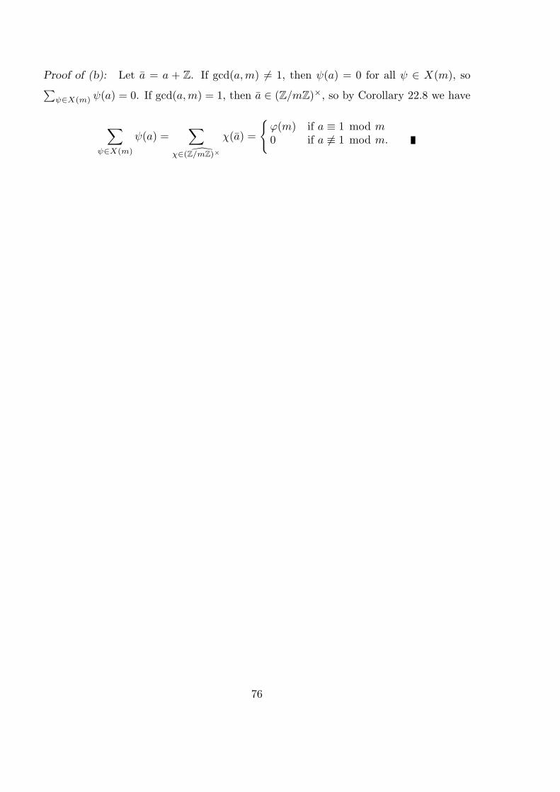
Proof of (b): Let a = a + Z. If gcd(a, m) 6= 1, then ψ(a) = 0 for all ψ ∈ X(m), so∑

ψ∈X(m) ψ(a) = 0. If gcd(a, m) = 1, then a ∈ (Z/mZ)×, so by Corollary 22.8 we have

∑

ψ∈X(m)

ψ(a) =∑

χ∈ (Z/mZ)×χ(a) =

{ϕ(m) if a ≡ 1 mod m0 if a 6≡ 1 mod m.

76

26. Euler Products EULERinput, 6

We apply the fundamental theorem of arithmetic to write Dirichlet series with ‘strongly

multiplicative’ coefficients as ‘Euler products’. Here we say that a function f : Z→ C is

strongly multiplicative if f(ab) = f(a)f(b) for all a, b ∈ Z.

Lemma 26.1: Let f : Z→ C be a strongly multiplicative function and let s be a complex EULainput, 14

number such that the series∑∞

n=1f(n)ns absolutely converges. Then the infinite product

∏p(1− f(p)p−s)−1, where p ranges over all prime number, converges and

(1)∞∑

n=1

f(n)ns

=∏p

1

1− f(p)ps

Proof: Let m be a natural number. By the fundamental theorem of number theory,

every natural number n whose prime divisors are at most m has a unique representation

as a product∏

p≤m pk(p) with non-negative integral exponents k(p). For such an n we

have f(n) =∏

p≤m f(p)k(p). Hence, by the absolute convergence,

∏

p≤m

1

1− f(p)ps

=∏

p≤m

(1 +f(p)ps

+f(p)2

p2s+

f(p)3

p3s+ · · ·) =

m∑n=1

f(n)ns

+∑n>m

′ f(n)ns

where the prime in the latter sum indicates that n ranges over all natural number greater

than m all of their prime divisors are at most m. It follows that

(2)∣∣∣∞∑

n=1

f(n)ns

−∏

p≤m

1

1− f(p)ps

∣∣∣ =∣∣∣

∑n>m

f(n)ns

−∑n>m

′ f(n)ns

∣∣∣ ≤∞∑

n=m+1

∣∣∣f(n)ns

∣∣∣.

By the absolut convergence, the series on the right hand side of (2) tends to 0 as m

tends to infinity. This implies that the infinite product comverges and that it is equal

to the infinite series as stated in the lemma.

Example 26.2: EULbinput, 62

(a) The Riemann zeta function ζ(s) =∑

n=11

ns absolutely converges when

Re(s) > 1. Since the constant function 1 is strongly multiplicative, the Euler formula

(3) ζ(s) =∏p

11− 1

ps

77

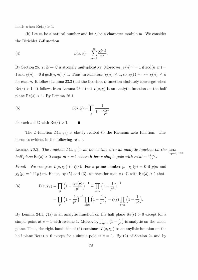
holds when Re(s) > 1.

(b) Let m be a natural number and let χ be a character modulo m. We consider

the Dirichlet L-function

(4) L(s, χ) =∞∑

n=1

χ(n)ns

.

By Section 25, χ: Z→ C is strongly multiplicative. Moreover, χ(n)m = 1 if gcd(n,m) =

1 and χ(n) = 0 if gcd(n,m) 6= 1. Thus, in each case |χ(n)| ≤ 1, so |χ(1)|+· · ·+|χ(n)| ≤ n

for each n. It follows Lemma 23.3 that the Dirichlet L-function abolutely converges when

Re(s) > 1. It follows from Lemma 23.4 that L(s, χ) is an analytic function on the half

plane Re(s) > 1. By Lemma 26.1,

(5) L(s, χ) =∏p

1

1− χ(p)ps

for each s ∈ C with Re(s) > 1.

The L-function L(s, χ1) is closely related to the Riemann zeta function. This

becomes evident in the following result.

Lemma 26.3: The function L(s, χ1) can be continued to an analytic function on the EULcinput, 109

half plane Re(s) > 0 exept at s = 1 where it has a simple pole with residue ϕ(m)m .

Proof: We compare L(s, χ1) to ζ(s). For a prime number p, χ1(p) = 0 if p|m and

χ1(p) = 1 if p - m. Hence, by (5) and (3), we have for each s ∈ C with Re(s) > 1 that

L(s, χ1) =∏p

(1− χ1(p)

ps

)−1

=∏

p-m

(1− 1

ps

)−1

(6)

=∏p

(1− 1

ps

)−1 ∏

p|m

(1− 1

ps

)= ζ(s)

∏

p|m

(1− 1

ps

).

By Lemma 24.1, ζ(s) is an analytic function on the half plane Re(s) > 0 except for a

simple point at s = 1 with residue 1. Moreover,∏

p|m(1− 1

ps

)is analytic on the whole

plane. Thus, the right hand side of (6) continues L(s, χ1) to an anylitic function on the

half plane Re(s) > 0 except for a simple pole at s = 1. By (2) of Section 24 and by

78

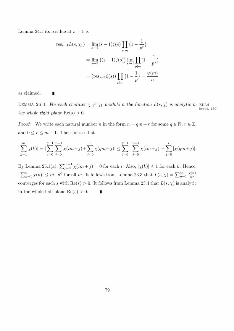
Lemma 24.1 its residue at s = 1 is

ress=1L(s, χ1) = lims→1

(s− 1)ζ(s)∏

p|m

(1− 1

ps

)

= lims→1

((s− 1)ζ(s)

)lims→1

∏

p|m(1− 1

ps)

=(ress=1ζ(s)

) ∏

p|m

(1− 1

p

)=

ϕ(m)n

as claimed.

Lemma 26.4: For each charater χ 6= χ1 modulo n the function L(s, χ) is analytic in EULdinput, 160

the whole right plane Re(s) > 0.

Proof: We write each natural number n in the form n = qm+ r for some q ∈ N, r ∈ Z,

and 0 ≤ r ≤ m− 1. Then notice that

|m∑

k=1

χ(k)| = |q−1∑

i=0

m−1∑

j=0

χ(im+j)+r∑

j=0

χ(qm+j)| ≤q−1∑

i=0

|m−1∑

j=0

χ(im+j)|+r∑

j=0

|χ(qm+j)|.

By Lemma 25.1(a),∑m−1

j=0 χ(im + j) = 0 for each i. Also, |χ(k)| ≤ 1 for each k. Hence,

|∑nk=1 χ(k)| ≤ m · n0 for all m. It follows from Lemma 23.3 that L(s, χ) =

∑∞n=1

χ(n)ns

converges for each s with Re(s) > 0. It follows from Lemma 23.4 that L(s, χ) is analytic

in the whole half plane Re(s) > 0.

79

27. Abscissa of Convergence ABSCISSAinput, 7

Following Lemma 23.2, we define the abscissa of convergence of a Dirichlet series

f(s) =∑∞

n=1an

ns as the infimum of all real numbers σ0 for which there exist t0 ∈ R such

that f(s) converges at s0 = σ0 + it0. By that lemma, −∞ ≤ α ≤ ∞ and f(s) converges

on the half plane Re(s) > σ0. By Lemma 23.4, f(s) is analytic on that half plane.

Lemma 27.1: Let f(s) =∑∞

n=1an

nsbe a Dirichlet series with non-negative real coeffi- ABSa

input, 19

cients an. Suppose the abscissa of convergence α of f(s) is a real number. Then s = α

is a singular point of f(s).

Proof: Let σ1 > α and present f(s) as a power series around s = σ1:

f(s) =∞∑

k=0

f (k)(σ1)k!

(s− σ1)k.

By what we wrote above, the sum converges in each s of the Disc D = {z ∈ C | |z| ≤σ1 − α} except possibly in s = α.

Assume by contradiction that s = α is a regular point of f(s). Then D1 is

contained in the regularity domain of f(s). In particular, f(s) is analytic in an open

disc around α. Therefore, the radius of convergence r of f(s) around σ1 is greator than

σ1 − α.

We choose ε > 0 such that r > σ1 − α + ε and note that (n−s)′ = (− log n)n−s,

so that the k’th derivative of f(s) =∑∞

n=1an

ns is

f (k)(σ1) =∞∑

n=1

(− log n)kan

nσ1.

Now we use that we may change the order of the summation in a double series with

non-negative real number and observe in the next computation that the Dirichlet series

80

∑∞n=1

an

nα−ε converges:∞∑

n=1

an

nα−ε=

∞∑n=1

an

nσ1· nσ1−α+ε

=∞∑

n=1

an

nσ1e(log n)(σ1−α+ε)

=∞∑

n=1

∞∑

k=0

(log n)k(σ1 − α + ε)k

k!

=∞∑

k=0

∞∑n=1

(log n)k(σ1 − α + ε)kan

k!nσ1

=∞∑

k=0

(α− ε− σ1)k

k!

∞∑n=1

(− log n)kan

nσ1

=∞∑

k=0

f (k)(σ1)k!

(α− ε− σ1)k = f(α− ε)

This contradicts the minimality of α.

Lemma 27.2: Let β ∈ R and let f(s) =∑n

n=1an

ns be a Dirichlet series with non-negative ABSbinput, 84

coefficients that converges on the half plane Re(s) > β. Suppose f(s) has an analytic

continuation to the half plane Re(s) > α for some α ≤ β. Then∑∞

n=1an

ns converges on

the half plane Re(s) > α.

Proof: Assume∑∞

n=1an

ns′ diverges for some s′ = σ′+it′ with σ′ > α. Then the abscissa

of convergence α′ of∑∞

n=1an

ns satisfies α′ ≥ σ′. By Lemma 27.1, α′ is a singular point

of f(s), in contrust to our assumption on f(s).

Lemma 27.3: Let f(s) =∑∞

n=1an

nsand g(s) =

∑∞n=1

bn

nsbe Dirichlet series with non- ABSc

input, 104

zero non-negative real coefficients an. Let α and β be the abscissas of convergence of

g and f respecitvely. Suppose −∞ < α ≤ β < ∞ and let h(s) = f(s)g(s) for each

s ∈ C with Re(s) > β. Then h(s) =∑∞

n=1cn

ns , where cn =∑

d|n adbn/d ≥ 0 for each n

is a representation of h(s) as a Dirichlet series and the abcissa of convergence of h is at

most β.

Proof: For each real σ > β both series∑∞

n=1an

nσ and∑∞

n=1bn

nσ are absolutely conver-

gent series. By a theorem of Cauchy, their product also absolutely converges, where the

nth term is cn

nσ with cn given as above. This conclude the proof.

81

28. Non-Vanishing of L(1, χ) NONVANISHinput, 8

A crucial point in the proof of Dirichlet’s theorem is the non-vanishing of L(1, χ) for

each non-principal character χ ∈ X(m). Here we follow Serre’s book “A course in

Arithmetic”. The proof circumvent delicate points of handling complex logarithm.

Again we fix a natural number m. If p - m, we let f(p) = ordmp. By Lemma

15.1(a), f(p)|ϕ(m). Let g(p) = ϕ(m)f(p) .

Lemma 28.1: For each natural number NONainput, 21

(1) 1−Xn =∏w

(1− wX),

where w ranges over all roots of Xn − 1 = 0 in C.

Proof: The complex roots of Xn − 1 form a multiplicative group W of order n. Both

sides of (1) are polynomials of order n having W as their set of roots. Indeed, when w

ranges over W , so does w−1 and 1− ww−1 = 0.

It follows that each w ∈ W is also the root of the polynomial

f(X) = (1−Xn)−∏

w∈W

(1− wX).

However, the free coeffient of both 1 −Xn and∏

w∈W (1 −mX) is 1. Hence, f(X) =

Xg(X), where g ∈ C[X] is a polynomial of degree n − 1. Moreover, w 6= 0 for each

w ∈ W , so g(w) = 0 for each w ∈ S. This contradicts Lemma 10.2 unless g = 0. Thus,

(1) is indeed an identity.

Lemma 28.2: If p - m, then NONbinput, 53

(2)∏

χ∈X(m)

(1− χ(p)X) = (1−Xf(p))g(p)

Proof: We apply Corollary 22.6 to the group B = (Z/mZ)× of order ϕ(m) and to

the element p = p + mZ whose order is f(p). By that Corollary, for each complex

root w of Xf(p) − 1 the number of characters χ of (Z/mZ)× such that χ(p) = w isϕ(m)f(p) . Hence, the number of characters χ ∈ X(m) such that χ(p) = w is g(p). Thus,∏

χ∈X(m)(1− χ(p)X) =(∏

w∈W (1− wX))g(p), where W now is the group of complex

82

roots of Xf(p) − 1 = 0. By Lemma 28.1,∏

w∈W (1−wX) = 1−Xf(p). Combining this

with the preceding equality, we get (2).

Lemma 28.3: The function ζm(s) defined for Re(s) > 1 by the formula NONcinput, 80

ζm(s) =∏

χ∈X(m)

L(s, χ)

has the multiplicative representation

ζm(s) =∏

p-m

1(1− 1

pf(p)s

)g(p).

Moreover, ζm(s) has a representation as a Dirichlet series with non-negative integral

coefficients that converges in the half plane Re(s) > 1.

Proof: By Examples 26.2(b) and by Lemma 28.2, we have for each s with Re(s) > 1,

ζm(s) =∏

χ∈X(m)

∏p

1

1− χ(p)ps

=∏

p-m

( ∏

χ∈X(m)

1− χ(p)p−s)−1

(3)

=∏

p-m

1(1− 1

pf(p)s

)g(p)=

∏

d|m

( ∏p-m

f(p)=d

11− 1

pds

)ϕ(m)/d

For each divisor d of m we define

hd(n) ={

0 if gcd(m, n) > 11 if gcd(m, n) = 1.

By Lemma 26.1,

(4)∏

p-m

11− 1

ps

=∏p

1

1− h(p)ps

=∞∑

n=1

h(n)ns

=∑

gcd(m,n)=1

1ns

and the right hand side is a Dirichlet series with non-negative integral coefficients

that converges when Re(s) > 1. Therefore, the same statement holds for the prod-

uct∏

p-m1

1− 1pds

for each divisor d of m. It follows from Lemma 27.3 that the right hand

side of (3) can be represented as a Dirichlet series with non-negative integral numbers

that converges for Re(s) > 1, as claimed.

83

Lemma 28.4: For each natural number m, the series∑

gcd(m,n)=11n diverges. HAR

input, 144

Proof: Observe that gcd(km + 1,m) = 1 and 2km ≥ km + 1 for each natural number

k. Hence,∑

gcd(m,n)=1

1n≥

∞∑

k=1

1km + 1

≥ 12m

∞∑

k=1

1k

.

Since the the harmonic series diverges, so does the series given in the lemma.

Proposition 28.5: L(1, χ) 6= 0 for every non-principal character modulo m. NONdinput, 162

Proof: By Lemma 26.3,

(5) L(s, χ1) =ϕ(m)

m(s− 1)+ f(s)

where f(s) is analytic at s = 1.

Assume there exists a non-principal character χ2 modulo m such that L(1, χ2) = 0.

By Lemma 26.4, L(s, χ2) is analytic at s = 1. Hence

(5) L(s, χ2) = b1(s− 1) + g(s)(s− 1)2

where g(s) is analytic at s = 1. Multiplying (5) and (6), we get

L(s, χ1)L(s, χ2) =ϕ(m)b1

m+ (b1f(s) +

ϕ(m)m

g(s))(s− 1) + f(s)g(s)(s− 1)2

is analytic at s = 1.

By Lemma 26.4, L(s, χ) is analytic at s = 1 for all non-principal characters modulo

m. Hence,

ζm(s) =∏

χ∈X(m)

L(s, χ) =(L(s, χ1)L(s, χ2)

) ∏

χ6=χ1,χ2

L(s, χ)

is analytic at s = 1. In addition, by Lemmas 26.3 and 26.4, for each χ ∈ X(m), the

function L(s, χ) is analytic at each s ∈ C with Re(s) > 0 and s 6= 1. It follows that

ζm(s) is analytic on the whole half plane Re(s) > 0.

Since ζm(s) has a presentation as a Dirichlet series with non-negative coeffients

on the half plane Re(s) > 1, it follows from Lemma 27.2 that the Dirichlet series

84

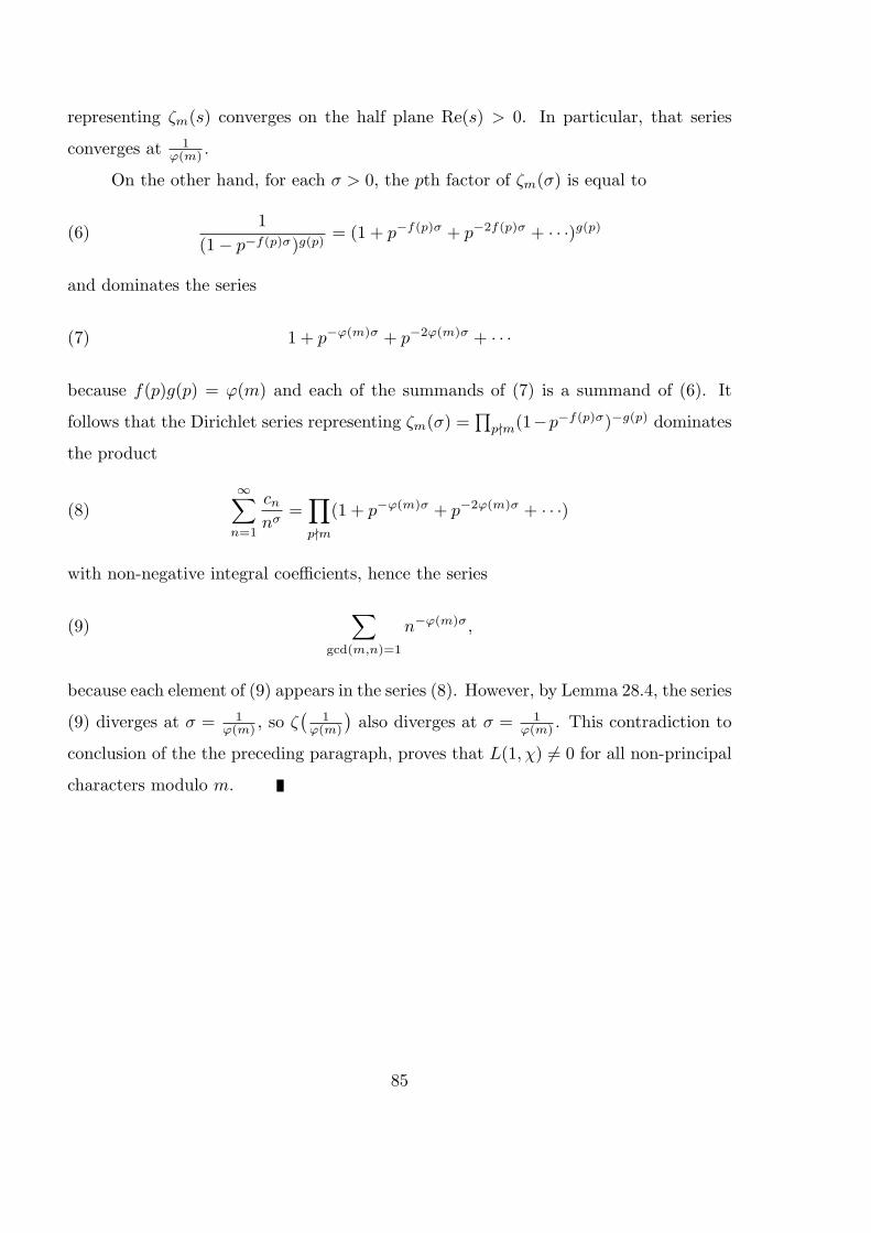
representing ζm(s) converges on the half plane Re(s) > 0. In particular, that series

converges at 1ϕ(m) .

On the other hand, for each σ > 0, the pth factor of ζm(σ) is equal to

(6)1

(1− p−f(p)σ)g(p)= (1 + p−f(p)σ + p−2f(p)σ + · · ·)g(p)

and dominates the series

(7) 1 + p−ϕ(m)σ + p−2ϕ(m)σ + · · ·

because f(p)g(p) = ϕ(m) and each of the summands of (7) is a summand of (6). It

follows that the Dirichlet series representing ζm(σ) =∏

p-m(1−p−f(p)σ)−g(p) dominates

the product

(8)∞∑

n=1

cn

nσ=

∏

p-m(1 + p−ϕ(m)σ + p−2ϕ(m)σ + · · ·)

with non-negative integral coefficients, hence the series

(9)∑

gcd(m,n)=1

n−ϕ(m)σ,

because each element of (9) appears in the series (8). However, by Lemma 28.4, the series

(9) diverges at σ = 1ϕ(m) , so ζ

(1

ϕ(m)

)also diverges at σ = 1

ϕ(m) . This contradiction to

conclusion of the the preceding paragraph, proves that L(1, χ) 6= 0 for all non-principal

characters modulo m.

85

29. Proof of Dirichlet’s Theorem LOGinput, 8

We define the Dirichlet density of a set A of prime numbers as the limit

(1) δ(A) = limσ→1+

∑p∈A

1pσ∑

p1

pσ

if it exists.

Theorem 29.1 (Dirichlet): Let m be a natural number and let a be a relatively prime LLGbinput, 23

integer to m. Then:

(a) limσ→1+∑

p1

pσ = ∞.

(b) The Dirichlet density of each finite set of prime numbers is 0.

(c) The Dirichlet density of the set of prime numbers p ≡ a mod m is 1ϕ(m) .

(d) There are infinitely many prime numbers p ≡ a mod m.

Proof: We break up the proof of the theorem into several parts.

Part A: A branch of the logarithm function. Recall that a branch of log z is a

continuous function l(z) defined on a connected open subset U of the complex plane

such that z = el(z) for each z ∈ U . If l1(z) is another branch of log z on U , then there

exists q ∈ Z such that l1(z) = l(z) + 2πi · q.By Proposition 28.5 L(1, χ) 6= 0 for each non-principal character χ modulo m.

Hence, we may choose a ray R in the left half plane Re(z) ≤ 0 starting at the origin

and passing through none of the points L(1, χ), where χ ∈ X(m) and χ 6= χ1. Let

D = CrR and choose a branch of log z which is analytic on D and coincides with the

usual real valued logarithm for each positive real number z. By the principal of analytic

continuation,

(2) − log(1− z) =∞∑

n=1

zn

n

if |z − 1| < 1 (becasue (2) holds for real numbers z satifying |z − 1| < 1). Moreover, if

z1, z2, z3, . . . is a sequence of complex numbers of absolute value less that 1, then

(3) l =∑∞

n=1 log(1− zn) converges if and only if∏∞

n=1(1− zn) converges.

86

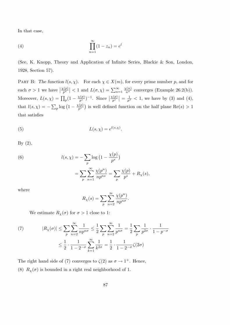
In that case,

(4)∞∏

n=1

(1− zn) = el

(See, K. Knopp, Theory and Application of Infinite Series, Blackie & Son, London,

1928, Section 57).

Part B: The function l(s, χ). For each χ ∈ X(m), for every prime number p, and for

each σ > 1 we have∣∣χ(p)

pσ

∣∣ < 1 and L(σ, χ) =∑∞

n=1χ(n)nσ converges (Example 26.2(b)).

Moreover, L(s, χ) =∏

p(1 − χ(p)ps )−1. Since

∣∣χ(p)ps

∣∣ = 1pσ < 1, we have by (3) and (4),

that l(s, χ) = −∑p log

(1 − χ(p)

ps

)is well defined function on the half plane Re(s) > 1

that satisfies

(5) L(s, χ) = el(s,χ).

By (2),

l(s, χ) = −∑

p

log(1− χ(p)

ps

)(6)

=∑

p

∞∑n=1

χ(pn)npns

=∑

p

χ(p)ps

+ Rχ(s),

where

Rχ(s) =∑

p

∞∑n=2

χ(pn)npnσ

.

We estimate Rχ(σ) for σ > 1 close to 1:

|Rχ(σ)| ≤∑

p

∞∑n=2

1npnσ

≤ 12

∑p

∞∑n=2

1pnσ

=12

∑p

1p2σ

· 11− p−σ

(7)

≤ 12· 11− 2−σ

∞∑

k=1

1k2σ

=12· 11− 2−σ

ζ(2σ)

The right hand side of (7) converges to ζ(2) as σ → 1+. Hence,

(8) Rχ(σ) is bounded in a right real neighborhood of 1.

87

Part C: The limit of l(s, χ) at s = 1. Consider χ ∈ X(m). Set ak = klogp k if k = pn

with p a prime number and n ∈ N. If k is not of the above form set ak = 0. Then,

|ak| ≤ 1 for each k (hence |∑nk=1 ak| ≤ n), and by (6), l(s, χ) =

∑∞k=1

ak

ks . By Lemmas

23.3 and 23.4, l(s, χ) is an analytic function on the half plane Re(s) > 1. It follows

from (5) that l(s, χ) is a branch of the log L(s, χ) on the half plane Re(s) > 1. It

follows that there exists a positive integer q(χ) such that c(χ) = 2pi · q(χ) satisfies

l(s, χ) = log L(s, χ) + c(χ).

If χ 6= χ1, then, by Lemma 26.4, L(s, χ) is analytic on the half plane. Moreover,

L(1, χ) ∈ D, so L(s, χ) ∈ D if s is sufficiently close to 1. Hence, in this case,

(9) log L(σ, χ) is analytic in an open neighborhood of 1, so limσ→1+ log L(σ, χ) =

log L(1, χ).

In particular, if χ 6= χ1, then by (9), l(s, χ) is analytic in an open neighborhood

of 1 and

(10) limσ→1+

l(s, χ) = l(1, χ).

Part D: An application of the orthogonality relation. Next we choose an integer a′

satisfying a′a ≡ 1 mod m. Then a′p ≡ 1 mod m if and only if p ≡ a mod m. Hence, by

Lemma 25.1(b),∑

χ∈X(m) χ(a′)χ(p) = ϕ(m) if p ≡ a mod m and∑

χ∈X(m) χ(a′)χ(p) =

0 if p 6≡ a mod m. Multiplying (6) by χ(a′), summing up over all characters χ modulo

n, we get

∑χ

χ(a′)l(σ, χ) =∑

p

1ps

∑χ

χ(a′)χ(p) +∑

χ

χ(a′)Rχ(s)(11)

= ϕ(m)∑

p≡a mod m

1ps

+ R∗(s),

where

(12) R∗(s) =∑

χ χ(a′)Rχ(s) is a bounded function in a right real neighborhood of 1.

By (6) in the proof of Lemma 26.3, el(s,χ1) = L(s, χ1) = ζ(σ)∏

p|m(1− 1

pσ

). Since

each of the numbers appearing in these equalities are real, we have, by (6), that

(13)∑

p

1pσ

+ Rχ1(σ) = l(s, χ1) = log ζ(σ) +∑

p|mlog

(1− 1

pσ).

88

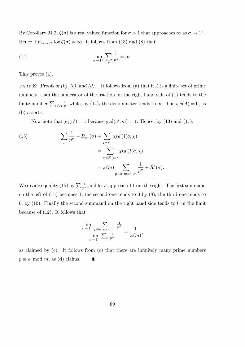
By Corollary 24.2, ζ(σ) is a real valued function for σ > 1 that approaches∞ as σ → 1+.

Hence, limσ→1+ log ζ(σ) = ∞. It follows from (13) and (8) that

(14) limσ→1+

∑p

1ps

= ∞.

This proves (a).

Part E: Proofs of (b), (c), and (d). It follows from (a) that if A is a finite set of prime

numbers, than the numerator of the fraction on the right hand side of (1) tends to the

finite number∑

p∈A1p , while, by (14), the denominater tends to ∞. Thus, δ(A) = 0, as

(b) asserts.

Now note that χ1(a′) = 1 because gcd(a′, m) = 1. Hence, by (13) and (11),

∑p

1pσ

+ Rχ1(σ) +∑

χ 6=χ1

χ(a′)l(σ, χ)(15)

=∑

χ∈X(m)

χ(a′)l(σ, χ)

= ϕ(m)∑

p≡a mod m

1pσ

+ R∗(σ).

We divide equality (15) by∑

1pσ and let σ approach 1 from the right. The first summand

on the left of (15) becomes 1, the second one tends to 0 by (8), the third one tends to

0, by (10). Finally the second summand on the right hand side tends to 0 in the limit

because of (12). It follows that

limσ→1+

∑p≡a mod m

1pσ

limσ→1+

∑p

1pσ

=1

ϕ(m),

as claimed by (c). It follows from (c) that there are infinitely many prime numbers

p ≡ a mod m, as (d) claims.

89

ELEMENTARY NUMBER THEORY - Tel Aviv Universityjarden/Courses/numb.pdf · ELEMENTARY NUMBER THEORY...

Documents

Transcript of ELEMENTARY NUMBER THEORY - Tel Aviv Universityjarden/Courses/numb.pdf · ELEMENTARY NUMBER THEORY...