Elementary Relativistic Wave Mechanics of Spin 0 and Spin 1/2 ...
Upload
jannah-ibrahimCategory
view
234download
0
8/8/2019 Elementary Micro Mechanics of Heterogeneous Media
http://slidepdf.com/reader/full/elementary-micro-mechanics-of-heterogeneous-media 1/166
Elementary Micromechanics of
Heterogeneous Media
Konstantin Z. Markov
“St. Kliment Ohridski” University of Sofia Faculty of Mathematics and Informatics 5 blvd J. Bourchier, P.O. Box 48 BG-1164 Sofia, Bulgaria [email protected]
Chapter 1 in the collection:
Heterogeneous Media: Modelling and Simulation,
edited by Konstantin Z. Markov and Luigi Preziosi, Birkhauser Bos-ton, 1999, pp. 1–162.
8/8/2019 Elementary Micro Mechanics of Heterogeneous Media
http://slidepdf.com/reader/full/elementary-micro-mechanics-of-heterogeneous-media 2/166
ii Heterogeneous Media: Modelling and Simulation
CONTENTS
1.1 Introduction 21.1.1 The Aim of Micromechanics . . . . . . . . . . . . . . . 21.1.2 The Idea of Homogenization . . . . . . . . . . . . . . . 4
1.1.3 Brief Historical Remarks . . . . . . . . . . . . . . . . . 7
1.1.3.1 Navier and Cauchy . . . . . . . . . . . . . . . . 81.1.3.2 Poisson and Mossotti . . . . . . . . . . . . . . . 91.1.3.3 Maxwell . . . . . . . . . . . . . . . . . . . . . . 11
1.1.3.4 Einstein . . . . . . . . . . . . . . . . . . . . . . 151.1.3.5 Smoluchowski . . . . . . . . . . . . . . . . . . . 17
1.1.4 The Outline of the Survey . . . . . . . . . . . . . . . . 18
1.2 The Homogenization Problem 211.2.1 The Representative Volume Element . . . . . . . . . . 221.2.2 Definition of the Effective Conductivity . . . . . . . . 25
1.2.3 Definition of the Effective Resistivity . . . . . . . . . . 28
1.2.4 Energy Definition of the Effective Constants . . . . . . 321.2.5 Consistency of the Definitions of Effective Properties . 351.2.6 The “Concentration” Factors . . . . . . . . . . . . . . 39
1.2.6.1 Ideal Thermal Contacts . . . . . . . . . . . . . 391.2.6.2 The Wu Representation . . . . . . . . . . . . . 421.2.6.3 Nonideal Thermal Contacts . . . . . . . . . . . 44
1.2.7 The Elastic Case . . . . . . . . . . . . . . . . . . . . . 451.2.7.1 The Basic Equations . . . . . . . . . . . . . . . 461.2.7.2 The Effective Elastic and Compliance Tensors . 471.2.7.3 The Elastic “Concentration” Factors . . . . . . 49
1.2.8 The Effective Absorption Coefficient . . . . . . . . . . 50
1.3 Some Basic Results 531.3.1 Weakly Inhomogeneous Media . . . . . . . . . . . . . . 54
1.3.1.1 The Definition . . . . . . . . . . . . . . . . . . 541.3.1.2 The Perturbation Expansion and the Second-
order Approximation . . . . . . . . . . . . . . . 551.3.1.3 The Third-order Approximation . . . . . . . . 58
8/8/2019 Elementary Micro Mechanics of Heterogeneous Media
http://slidepdf.com/reader/full/elementary-micro-mechanics-of-heterogeneous-media 3/166
Micromechanics of Heterogeneous Media iii
1.3.2 The Hashin-Shtrikman Estimates . . . . . . . . . . . . 601.3.2.1 The Bergman Formula . . . . . . . . . . . . . . 611.3.2.2 The Matheron Inequalities . . . . . . . . . . . . 621.3.2.3 The Wiener Bounds . . . . . . . . . . . . . . . 631.3.2.4 The Hashin-Shtrikman Bounds . . . . . . . . . 64
1.3.3 The Hashin Assemblage . . . . . . . . . . . . . . . . . 661.3.4 The Variational Estimates . . . . . . . . . . . . . . . . 68
1.3.4.1 The Dirichlet Principle . . . . . . . . . . . . . . 681.3.4.2 The Thompson Principle . . . . . . . . . . . . 691.3.4.3 The Beran Bounds . . . . . . . . . . . . . . . . 70
1.3.4.4 The Torquato-Milton Patameter . . . . . . . . 751.3.5 The Bounds in the Elastic Case . . . . . . . . . . . . . 771.3.6 Cross-properties Relations: The Levin Formula . . . . 801.3.7 The Elementary Bounds on the Effective Absorption
Coefficient . . . . . . . . . . . . . . . . . . . . . . . . . 83
1.4 The Single Inclusion Problem 851.4.1 Scalar Conductivity—Integral Equation . . . . . . . . 851.4.2 Scalar Conductivity—Ellipsoidal Inhomogeneity . . . . 861.4.3 Singular Inclusions and Nonideal Contacts . . . . . . 86
1.4.3.1 Singular Inclusions . . . . . . . . . . . . . . . . 92
1.4.3.2 Nonideal Contacts . . . . . . . . . . . . . . . . 931.4.3.3 The “Superconducting” Spherical Inhomogene-ity . . . . . . . . . . . . . . . . . . . . . . . . . 94
1.4.3.4 The “Resisitive” Spherical Inhomogeneity . . . 961.4.4 Elastic Case . . . . . . . . . . . . . . . . . . . . . . . . 99
1.5 One-particle Approximations 1051.5.1 Dilute Filler Fraction—Scalar Conductivity . . . . . . 1061.5.2 Dilute Filler Fraction—Elastic Case . . . . . . . . . . 1101.5.3 Self-consistent Scheme . . . . . . . . . . . . . . . . . . 113
1.5.3.1 The Basic Idea . . . . . . . . . . . . . . . . . . 1131.5.3.2 An Alternative Derivation . . . . . . . . . . . . 1131.5.3.3 The Percolation Phenomenon . . . . . . . . . . 1171.5.3.4 Some Particular Cases of the Self-consistent
Scheme . . . . . . . . . . . . . . . . . . . . . . 1181.5.4 The Differential Scheme . . . . . . . . . . . . . . . . . 120
1.5.4.1 The Basic Idea . . . . . . . . . . . . . . . . . . 1211.5.4.2 Some Particular Cases . . . . . . . . . . . . . . 122
8/8/2019 Elementary Micro Mechanics of Heterogeneous Media
http://slidepdf.com/reader/full/elementary-micro-mechanics-of-heterogeneous-media 4/166
iv Heterogeneous Media: Modelling and Simulation
1.5.5 The Effective Field . . . . . . . . . . . . . . . . . . . . 1251.5.5.1 The Basic Idea . . . . . . . . . . . . . . . . . . 1261.5.5.2 Alternative Derivations and Interpretations . . 1271.5.5.3 Some Particular Cases . . . . . . . . . . . . . . 128
1.5.6 The Conductivity of a Medium with Non-ideal Inter-phase Contacts . . . . . . . . . . . . . . . . . . . . . . 133
1.5.7 The Self-consistent Scheme for the Absorption Problem 135
1.6 Elastic Properties of Polycrystals 1391.6.1 The Self-consistent Scheme for Polycrystals . . . . . . 139
1.6.2 Formulation in Compliances and Consistency of theScheme . . . . . . . . . . . . . . . . . . . . . . . . . . 142
1.6.3 Example: Elastic Moduli of a Cubic Polycrystal . . . . 143
1.7 References 146
8/8/2019 Elementary Micro Mechanics of Heterogeneous Media
http://slidepdf.com/reader/full/elementary-micro-mechanics-of-heterogeneous-media 5/166
1
Elementary Micromechanics of
Heterogeneous Media
Konstantin Z. Markov
“St. Kliment Ohridski” University of Sofia
Faculty of Mathematics and Informatics
BG-1164 Sofia, Bulgaria
Abstract. The introductory and more elementary ideas and re-sults of micromechanics of heterogeneous media are collected in thesurvey. The central problem under discussion is “homogenization.”It replaces such media by homogeneous ones, which behave macro-scopically in the same way and possess certain gross effective prop-erties. These properties are related in a complicated manner to theprescribed internal structure of the medium and their evaluation, ingeneral, represents a profound challenge in any specific situation. Abrief historical survey is given, underlying the reappearance of es-sentially the same “homogenization” quest in numerous guises andcontexts over the last two centuries. Within the framework of the
volume-averaging approach the basic notions are introduced and someof the central, now classical, results are then derived and discussedsuch as perturbation expansions, Hashin-Shtrikman’s bounds, varia-tional estimates and Levin’s cross-property relation. A general “one-
1
8/8/2019 Elementary Micro Mechanics of Heterogeneous Media
http://slidepdf.com/reader/full/elementary-micro-mechanics-of-heterogeneous-media 6/166
2 Heterogeneous Media: Modelling and Simulation
particle” scheme for approximate evaluation of the effective properties(in the static case) is detailed in its various implementations like self-consistency, iterated limits and effective field. Illustrations concernconductivity, elasticity, and absorption phenomena in heterogeneousparticulate media, as well as a simple self-consistent model for poly-crystals’ homogenization.
1.1 Introduction
1.1.1 The Aim of Micromechanics
Continuum mechanics deals with ideal homogeneous materials. Itsaim is to describe their response to external exertions using appropri-ate constitutive relations. The latter generally are specified by meansof macroscopical experiments without microstructural considerations.It is a trivial statement, however, that any sample of material is mi-croscopically inhomogeneous, even if it appears homogeneous at somenatural scale of observation. Inevitably, therefore, a description of any material in terms of continuum mechanics is an approximation,
and any experimental determination of constitutive behavior yields,in fact, a relationship between the “overall” properties measured inthe experiment. This observation leads us to a fundamental andwidespread problem of science and technology, concerning “micro-macro” interconnection, i.e. a proper and reliable determination of the macroscopic (or “large” scale) behavior of a medium which ex-hibits microscopic (or “small” scale) heterogeneity, on the base of the appropriate and available microstructural information. (The ex-act meaning of “large” and “small” depends on the specific problemsand media under study.) The oldest problem of such a type, fun-damental in statistical physics, is description of matter in terms of its molecular constituents. Here “small” corresponds obviously tomolecular dimensions.
Micromechanics, in general, deals with heterogeneous media forwhich “small” has a certain intermediate dimension which is largecompared to molecular dimensions, but is small in macroscale. Thelength is connected with the characteristic size of the heterogeneitiesin the medium, say, with mean radius of inclusions, voids, fibers, the
8/8/2019 Elementary Micro Mechanics of Heterogeneous Media
http://slidepdf.com/reader/full/elementary-micro-mechanics-of-heterogeneous-media 7/166
1.1 Micromechanics of Heterogeneous Media 3
size of a crystallite in polycrystalline aggregates, etc. Though themolecular effects are not present, as a rule, in such a scale, many of the methods used in the appropriate theories have their direct ori-gin in statistical physics and statistical mechanics, as we shall pointout below. The aim of micromechanics is just to relate the grossmacroscopical behavior of heterogeneous media, characterized withthe above mentioned length scale , to the details of their microscop-ical constitution. The basic idea is that of homogenization, whichconsists in a replacement of a piece of a microheterogeneous solidby a homogeneous one which, from a macroscopical point of view
“behaves” in the same manner as this piece. This fundamental ideawill be briefly illustrated in the next subsection, before considering itmore rigorously and in needed detail in Section 1.2.
Note that an important class of heterogeneous media, extensivelytreated by micromechanics, are the composites—man-made mixturesmixtures of two or more constituents, firmly (as a rule, but not al-ways) bonded together. Among other reasons, technological demandshave stimulated a very extensive bulk of studies, devoted to theirgross mechanical behavior, like elasticity, strength, etc., as predefinedby a specific microstructural arrangement. A considerable part of themore fundamental works along this line will be discussed in what fol-
lows. There are, however, plenty of micromechanical problems notdirectly concerned with mechanical properties, but representing par-ticular cases of the same “micro-macro” interconnection quest, inwhich the same idea of homogenization applies.1 An example is fur-nished by the problem of describing propagation of electromagneticor acoustic waves through a heterogeneous solid or a turbulent fluid.Another example is cooling of a heated body by means of a system of tubes or holes, kept at a fixed temperature. Mathematically the lat-ter problem is very closely connected to describing the gross behaviorof a diffusing species in a medium, containing absorbing sinks. The
1It is more precise perhaps to speak about “micro-physical” problems, instead
of micromechanical since, say, diffusion, electromagnetic waves, etc., have little todo with mechanics in its classical sense. However, introducing the term physicswould inevitably enlarge this survey far beyond the admissible length and (moreimportant)—the author’s competence. In this connection it seems appropriate torecall the Constitution of the International Society for the Interaction of Mechanicsand Mathematics (ISIMM), where one reads that “Mechanics is understood here
in the broad sense of the word, including relevant physical phenomena such as
electromagnetic and thermal fields.”
8/8/2019 Elementary Micro Mechanics of Heterogeneous Media
http://slidepdf.com/reader/full/elementary-micro-mechanics-of-heterogeneous-media 8/166
4 Heterogeneous Media: Modelling and Simulation
third example to be specially mentioned concerns the viscous flowthrough a porous solid (which itself could deform due to the flow).
1.1.2 The Idea of Homogenization
To illustrate the basic ideas of homogenization as simply as possible,consider a (linear) elastic heterogeneous medium. Let, for example,the tensile stress-strain behavior of the medium along the axis x1 beunder investigation. Imagine to this end that a large, say, cubicalspecimen V with a side L is cut out from the medium; large meanshere that L
, where is the above mentioned microscale length.
Either the cube would be loaded to some level and its extension mea-sured, or else it would be extended by some amount and the loadmeasured. Then the stress component σ11 would be taken as loaddivided by area of the cross-section L2 and the strain component ε11
as extension divided by the original length L. These two ways to findε11 and σ11 are obvious, if the cube were homogeneous; the hetero-geneity results, however, in non-homogeneous and rapidly oscillatingin the microscale fields of both stress and strain. The latter quanti-ties, calculated from the experiment, thus represent, in fact, averagesof the actual forces and displacements in the cube. More precisely,they are just the so-called volume (or spatial) averages, to be denoted
by overbar:
ε11 =1
V
V
ε11(x) dx , σ11 =1
V
V
σ11(x) dx ; (1.1)
hereafter V = vol V is the volume of the region V .In turn, the proportionality coefficient
E V 11 = σ11 / ε11 (1.2)
defines the effective (or gross) Young modulus for the specimen (alongthe axis x1). This means that the cube, through the relation (1.2),is “homogenized” in the sense that its heterogeneity is smoothed outand it is replaced by a homogeneous one, possessing the gross Youngmodulus E V 11.
If we now repeat the same procedure for other cubical samples of the material, of the same size and orientation as the first, we shall ingeneral obtain slightly different values of E V 11, since the interior phasegeometry will not be the same in full detail. This explains why thesuperscript ‘V ’ explicitly appeared in the notation E V 11.
8/8/2019 Elementary Micro Mechanics of Heterogeneous Media
http://slidepdf.com/reader/full/elementary-micro-mechanics-of-heterogeneous-media 9/166
1.1 Micromechanics of Heterogeneous Media 5
To define a “true” material property from such experiments, i.e.one that is connected with the heterogeneous medium and its internalstructure, independently of the specific choice of the subvolumes, twonatural procedures can be employed.
First, perform a great number, N , of experiments on differentlycentered cubes (otherwise identical and identically oriented), andmeasure the appropriate values E V
11 , E V
11 , etc., for each one. Then,to suppress the specimen’s dependence, it is natural to define
E ∗11 =1
N E V
11 + E V
11 +
· · · , (1.3)
which is already a true material property. The right-hand side of (1.3) is the simplest example of the so-called ensemble averaging .The meaning is that to obtain information about the expected grossbehavior of a heterogeneous medium, we should deal with averagereaction of a whole ensemble of specimens of identical shape and size,and apply identical external influence. (In the foregoing reasoningthese are simply the cubes taken from different parts of a big pieceof the medium.) The ensemble averaging is one of the basic notionin the theory of heterogeneous media of random constitution, see e.g.the book of Beran [BEi]. An elucidating introduction, together with
basic methods and ideas concerning homogenization for such randommedia, can be found as well in the lectures of Willis [WIe].
We shall be concerned in the present survey, however, with moreelementary aspects of the theory, without invoking the proper math-ematical framework for random internal constitution. That is whyonly the volume averaging (1.1) will be used throughout. It appearsin a natural way, if a second kind of mental experiment is performed.Take a cube with a fixed center and start increasing its side L (as-suming the medium unbounded). Then it is equally natural to expectthat in the limit L/ → ∞ the sample dependence will disappear:
E V 11
= E ∗11
(1 +O
(/L)) as /L→
0 , (1.4)
where the same effective modulus E ∗11, as in (1.3), shows up. Hence,we shall be on the safe side, equating E ∗11 with E V 11, provided thevolume V is big enough compared to the typical inhomogeneity, i.e. if L . But this was a basic assumption, already adopted for theclass of heterogeneous media under study at the beginning of this
8/8/2019 Elementary Micro Mechanics of Heterogeneous Media
http://slidepdf.com/reader/full/elementary-micro-mechanics-of-heterogeneous-media 10/166
6 Heterogeneous Media: Modelling and Simulation
subsection. The importance of this assumption will be once moreemphasized in Section 1.2.1, when formulating Hashin’s MMM prin-ciple.
Hereafter we shall consider only media for which the ensemble andvolume averages coincide; they are called ergodic .
A satisfactory proof of the statement that a medium is ergodic,i.e. the two definitions (1.3) and (1.4) yield, in particular, one and thesame value of E ∗11 is not a trivial matter. Such a statement amountsto the so-called ergodic hypothesis . It can be rigorously justifiedunder certain additional conditions imposed on the microgeometry
of the media, the most important of which is the macroscopic (orstatistical) homogeneity, see again the book [BEi] for a brief, butelucidating discussion.
Intuitively, the coincidence between the ensemble and volume av-erages should not be a surprise, since E ∗11 is to be specified by themedium’s microgeometry solely. Any natural definition of the ho-mogenization properties, in which sample dependence is somehoweliminated, should then result in a true and unique material charac-teristics.
Fully similar considerations can be repeated almost literally, usingdifferent physical backgrounds, chosen and tailored by the personal
taste of the reader. For example, instead of elasticity, diffusion of asolute through the same cube V can be considered, fixing the soluteconcentration at a pair of opposite faces and, in the steady state,measuring the total amount of the solute, passing through them, see[HUa]. The dielectric context is also used very often, starting withthe classical works of Mossotti [MOc], [MOd], and Faraday [FAa];the posing of the homogenization problem in this case is very clearlyexplained and discussed, e.g. by Bergman [BEk]. A fully equivalent,from a mathematical point of view, context concerns heat propaga-tion which will be mainly used in what follows. That is why we shouldrecall here the well-known equations
· q(x) = 0 , q(x) = κ(x)θ(x) , (1.5)
that govern the temperature field θ(x) in a medium at the absence of body sources. In Eq. (1.5) q(x) is the flux vector, and κ(x) represents,for the heterogeneous body under study, a rapidly fluctuating con-ductivity coefficient, taking different values when the point x scans
8/8/2019 Elementary Micro Mechanics of Heterogeneous Media
http://slidepdf.com/reader/full/elementary-micro-mechanics-of-heterogeneous-media 11/166
1.1 Micromechanics of Heterogeneous Media 7
the medium. In the case of a two-phase (binary) material, which veryoften appear in various applications,
κ(x) =
κ1, if x ∈ constituent ‘1’,
κ2, if x ∈ constituent ‘2’.(1.6)
It should be emphasized that all the results, obtained below in theheat conduction context, are equally well applicable in the contexts of electrical conductivity, dielectric behavior and magnetic permeability.A list of analogous quantities are conveniently summarized in a table
by Hashin [HAi, p. 496]. The reason is the obvious mathematicalsimilarity between between these problems: in all of them a solenoidalvector field (say, the dielectric polarizability, or the heat flux, etc.)is “proportional” to a potential vector field (the electric field, thetemperature gradient, etc.) with a proportionality coefficient (whichmay be a tensor) rapidly varying throughout the medium.
The second context to be more extensively used in the present pa-per is the already employed, for illustrative purposes, (linear) elastic-ity problem (see Section 1.2.7 below). The basic ideas and conclusionsare the same in both cases, but their implementation in the heat con-ductivity case is, however, simpler, since the basic quantities—theheat flux and temperature gradient—are vectors. In the elasticitycase the respective quantities are tensors (the stress and strain ones)which makes the calculations more cumbersome technically. Thatis why we shall concentrate in what follows primarily on the scalarconductivity problem; afterward, the elasticity counterparts of theresults will be discussed more concisely.
1.1.3 Brief Historical Remarks
The homogenization quest, due to its utmost importance, has keptreappearing in various guises and contexts in the last two centuries,attracting the interest and the efforts of some of the most illustriousnames in science. Here we shall try to collect some historical de-tails, without any attempt or claim to be full and exhaustive.2 Oneof our aims is to underline the common “micromechanical” origin
2We do not mention even the famous Darcy’s book [DAa] that initiated tremen-dous research on flow in porous media, and on Darcy’s law, in particular. A greatnumber of recent developments in this field can be found in other papers of thepresent volume.
8/8/2019 Elementary Micro Mechanics of Heterogeneous Media
http://slidepdf.com/reader/full/elementary-micro-mechanics-of-heterogeneous-media 12/166
8 Heterogeneous Media: Modelling and Simulation
and nature of the appropriate problems, despite the widely differentscientific communities and contexts in which they have shown up.
1.1.3.1 Navier and Cauchy
It should be recalled above all that the origin and the base of themodern continuum mechanics, as laid down by Navier and Cauchy,is to a great extent “micromechanical.” The starting point of theseauthors was the Newtonian picture of matter as an assemblage of “material molecules” interacting by means of central forces. In a lan-guage, used today, this is nothing but a “discrete” model and theirmain and great contribution in this field is the “homogenization” of such a model. More precisely, imaging the “molecules” as materialpoints and the interaction forces depending upon their displacementfrom the equilibrium position, first Navier and then, almost in thesame time and in a more general form, now classical, Cauchy de-rived3 the equations describing an elastic continuum, “spread over”the discrete model—in the sense that it macroscopically behaves inthe same way as its underlying “molecular skeleton.” This discretemodel was then put aside for more than a century and the attention,in continuum mechanics at least, was focused on the appropriate par-tial differential equations that formed, together with the equations of
hydrodynamics, the core of research in the Mathematical Physics of the previous century.
In a new guise and on a new level, similar “homogenization” prob-lems reappeared in continuum mechanics almost a century later whenEinstein [EIa] in 1905 and Bruggeman [BRg] in 1937 considered hostsof inclusions in a fluid and in an elastic medium, respectively. In bothcases the problems were again micromechanical, in the sense that ho-mogeneous continua, spread over discrete arrays of inclusions, shouldbe constructed. The interpretation of “micro” was of course differ-ent from the pioneering works of Navier and Cauchy, but the senseof the “homogenization” quest was the same. However, the nature
of interaction between the inclusions exhibited a key new feature:3According to Love [LOd] (see the historical survey in his introduction), the
Navier Memoire was presented at the French Academy in May 1821, but waspublished only in 1827 [NAa]. The Cauchy Memoire was presented at the FrenchAcademy in September 1821, but also appeared in 1827 and 1928 in his Exercises
de mathematique . The Cauchy derivation revisited can be found in Appendix Bof the same Love book [LOd].
8/8/2019 Elementary Micro Mechanics of Heterogeneous Media
http://slidepdf.com/reader/full/elementary-micro-mechanics-of-heterogeneous-media 13/166
1.1 Micromechanics of Heterogeneous Media 9
its magnitude already was not prescribed, like a simple elastic one,say, but instead resulted from the local disturbances of the fields likedisplacement, velocity, etc., generated by each single particle in themedium.
1.1.3.2 Poisson and Mossotti
With elastic bodies “homogenized,” the micromechanical studies of heterogeneous media for almost a century turned toward the grossbehavior of charged materials.4
In 1824 Poisson presented his first Memoire on the theory of mag-netism at a meeting of the French Academy [POa]. There he putthe basis of the theory of induced magnetism, assuming a model of a nonconducting material (we would call it a matrix today) in whichsmall conducting particles are distributed. For magnetically isotropicbodies Poisson took the particles spherical, isotropically arranged aswell, and noted that an adequate theory of magnetism can be con-structed if one requires that each sphere is lying in a certain constantexternal field. In his second Memoire [POb], he treated anisotropicmagnetic solids as well, representing them as an array of thin alignedthree-axial conducting ellipsoids in a matrix. In these two Poisson’spapers one can see not only the origin but the rudiments of the basic
models and ideas that prevailed in the theory of heterogeneous me-dia for almost a century after their appearance, and are still usefuland applicable. In particular, the model of the so-called dispersion of nonoverlapping spheres and ellipsoids seems to have emerged for thefirst time in this particular (magnetic) context; the model, in gen-eral, turned out very appropriate for many heterogeneous media of particulate type (matrix-inclusion composites, say), and also in theliquid-state theory.
It was Faraday in 1838 [FAa], who employed Poisson’s ideas todielectrics, proposing to treat them as an array of metallic spheres,immersed into an insulating material (matrix) [FAa]. But a more
detailed analysis of this model was due to Mossotti [MOc] who spec-ified the embedded particles as “material molecules,” modelled themas little conducting spheres, and described the polarization of a sin-gle one. The main contribution of Mossotti was however a method
4In the “electric” story we shall utilize a number of historical details, given byWiener [WIa], Brown [BRe], Landauer [LAc] and Trimarco [TRa].
8/8/2019 Elementary Micro Mechanics of Heterogeneous Media
http://slidepdf.com/reader/full/elementary-micro-mechanics-of-heterogeneous-media 14/166
10 Heterogeneous Media: Modelling and Simulation
of interconnecting the micro- and macroproperties of the dispersionwhich turned out to be the first of the so-called “cavity” approaches,and this was the heart of his second paper [MOd]. The basic, andextremely fruitful, idea of Mossotti was to remove a material region Caround a point in order to evaluate the (electric) force exerted on thepoint, due to the interactions with the molecules outside C. In thisway the first of the “cavity” methods in theory of heterogeneous me-dia emerged. The field acting on the cavity is the local (or effective,or internal) field that differs from the applied macroscopic one, as aconsequence of the presence of the other molecules. In Section 1.5.3
below, when discussing the so-called effective field approach for evalu-ating the effective properties, we shall specially outline its connectionwith the “cavity” idea, see Section 1.5.5.2. As pointed out by Lan-dauer [LAc], the Mossotti work [MOd] is based, however, on etherialconcepts and notions, typical for the epoch, which makes this clas-sical paper difficult for a modern reader to follow. The idea of localfield was reintroduced and exploited by H. Lorentz around 1880. Avery clear and now classical exposition of this idea and its applicationto dielectric and optical properties5 is given in his well-known book[LOb, Section 117 and App. 54].
Almost at the same time Clausius in his book [CLa, pp. 67–77]
revisited Mossotti’s internal field approach in a concise way, mucheasier for a modern reader to follow [LAc]. He cut each moleculeout of the medium and replaced the rest with a material possessingthe effective dielectric constant, reaching the explicit and now clas-sical formula for the latter, given in Eq. (1.19) below. This is, as amatter of fact, the first appearance of the so-called effective mediumidea that much later was successfully exploited by Bruggeman, Sko-rohod, Hill, Budiansky et al. in the theory of heterogeneous solids,see Section 1.5.2 below. As pointed out by Brown [BRe], Mossotti’spaper does not contain explicitly the formula for the effective dielec-tric constant; Clausius’ book does, and that is why H. Lorentz [LOb,
Section 124] attributes the formula (1.19) to Clausius and Mossotti,5Recall that according to Maxwell, µ2 = κ, where κ is the dielectric constant
of a transparent medium and µ = c/v is its refractivity index (i.e. the ratio c/vbetween the velocity of the light in the vacuum and in the medium). This clas-sical formula of the electromagnetic theory explains the appearance of equivalentformulae for the effective properties, containing refractivity instead of dielectricproperties.
8/8/2019 Elementary Micro Mechanics of Heterogeneous Media
http://slidepdf.com/reader/full/elementary-micro-mechanics-of-heterogeneous-media 15/166
1.1 Micromechanics of Heterogeneous Media 11
and it has come to be known as the Clausius-Mossotti’s one. Butseveral years before Clausius’ publication, an analogous formula inconductivity had been given by Maxwell [MAj], whose reasoning willbe presented below.
Note also that L. Lorenz in three papers between 1869 and 1880considered optical problems, concerned with propagation of electro-magnetic waves (“optical vibrations” as he called them) [LOc]. Heassigned a refractive index to each molecule that differs from thatof the surrounding medium and then employed a scheme which re-sembled very much what is now called the Coherent Potential Ap-
proximation. That is why the local field and its expression, to bediscussed in an appropriate context in Section 1.5.5.1, is often calledLorenz-Lorentz’s field.
1.1.3.3 Maxwell
In his famous treatise [MAj] Maxwell addressed in passing the prob-lem of predicting the overall behavior of a dispersion of spheres, im-mersed into a matrix of different conductivity. We shall repeat herehis elegant and simple reasoning, since it contains a number of basicideas and drawbacks that have kept reappearing in the later worksfor a long period afterward.
The basic building block in Maxwell’s study is the single spherefield. Let a single spherical inhomogeneity V a, located at the origin,be immersed into an unbounded matrix. Let the applied far-fieldhave a constant and prescribed gradient, i.e. θ∞(x) = G · x. Thetemperature field, θ(x), is governed then by the equation:
· (κ(x)θ(x)) = 0 , θ(x) → G · x as |x| → ∞ ,
κ(x) = κ1 + [κ]ha(x) , [κ] = κ2 − κ1 ,(1.7)
where ha(x) is the characteristic function of the sphere V a, κ1 and κ2
are the conductivities of the matrix and of the sphere, respectively,see Eqs. (1.5) and (1.6).
Since κ(x) is a step-constant function, the field θ(x) should be aharmonic function both inside and outside the sphere; on the spheresurface, |x| = a, it should be continuous together with the normalcomponent of the heat flux:
κ2∂θ
∂r
r=a−0
= κ1∂θ
∂r
r=a+0
, (1.8)
8/8/2019 Elementary Micro Mechanics of Heterogeneous Media
http://slidepdf.com/reader/full/elementary-micro-mechanics-of-heterogeneous-media 16/166
12 Heterogeneous Media: Modelling and Simulation
as it follows directly from (1.7); here r = |x| is the radial coordinate,a is the sphere’s radius.
The solution of Eq. (1.7) depends linearly on the far-field gradientG. Together with the obvious geometrical symmetry, this suggeststo look for the needed solution in the form
θ(x) = G · ϕ(r) . (1.9)
Since θ(x) is harmonic, Eq. (1.9) implies
∆θ(x) = G · ∆ϕ(r) = 0 , i.e. ∆ϕ(r) = const ,
and henceϕ(r) = 1
2 C r2 − C a/r + const . (1.10)
Obviously, the additive constant in the last formula does not influencethe solution (1.9). Inside the sphere C = 0, in order to have abounded everywhere solution there, so that
θ(x) = C G · x , |x| < a . (1.11)
Outside the sphere C = 1, in order to meet the far-field condition inEq. (1.7), and hence
θ(x) = G · x 1 − C (a/r)3
, |x| > a . (1.12)
The continuity conditions for θ(x) and for the normal flux at |x| =a, see Eq. (1.8), yield
C = 1 + C , κ2C = κ1(1 − 2C ) ,
as it follows from Eqs. (1.11) and (1.12), and also from the simpleformula
∂θ
∂r= er · θ(x) = G · ϕ(r) · er = ϕ(r)G · er , (1.13)
er = x/r, r = |x|, which holds for any function of the form (1.9).The solution of the single inclusion problem (1.7) therefore reads
θ(x) = G · x γ , if |x| < a ,
1 − β (a/r)3 , if |x| > a ,(1.14)
with the constants
β =[κ]
κ2 + 2κ1, γ = 1 − β =
3κ1
κ2 + 2κ1. (1.15)
8/8/2019 Elementary Micro Mechanics of Heterogeneous Media
http://slidepdf.com/reader/full/elementary-micro-mechanics-of-heterogeneous-media 17/166
1.1 Micromechanics of Heterogeneous Media 13
Remark 1.1 In Section 1.4.2 we shall find the solution of Eq. (1.7)inside the sphere in a much simpler way, which works equally well for an ellipsoidal inhomogeneity also. In Maxwell’s considerations one needs, however, the field θ(x) outside the sphere, so that a more lengthy analysis is required.
Remark 1.2 The formula (1.14) shows that if the temperature gra-dient at infinity is constant, the same holds true for this gradientinside a spherical inhomogeneity. This is a particular case of a more general statement in which the sphere is replaced by an ellipsoidal in-
homogeneity. A similar statement holds for the elastic inhomogeneity problem, see Section 1.4.4.
With the single-sphere solution found, we can go back to Maxwell’sanalysis. Consider a large sphere V A of the radius A and conductiv-ity κ1, containing N identical and nonoverlapping small spheres of conductivity κ2. (“Large” means here that A a, where a is theradius of the small spheres.)
Immerse the sphere V A into a homogeneous medium possessing thesame conductivity κ1 as that of the matrix. “Sit down” at the pointM , far away from the center O of the sphere, i.e. imagine R A,where R =
|OM
|. Assume again that the temperature gradient G at
infinity is constant. The presence of the inhomogeneous sphere V Awill disturb the field G·x that would have existed in the homogeneousmedium of conductivity κ1 at its absence. We shall evaluate thisdisturbance in two different ways.
First, let us consider each small sphere within V A as a single andpretend there are no other small spheres around it. Then, accord-ing to Eq. (1.14), the disturbance, caused by any such sphere, is−βa3/R3, and summing up all of them, gives
−Nβ a3
R3= −N
a3
R3
κ2 − κ1
κ2 + 2κ1; (1.16)
recall that the small spheres within V A are located practically at oneand the same distance R from our observation point M , since R A.
Second, “looking” at the big sphere V A from a great distance, wecan “homogenize” it, neglecting its heterogeneous internal structureand replacing it by a homogeneous sphere possessing a certain un-known effective conductivity κ∗. The disturbance, caused by such a
8/8/2019 Elementary Micro Mechanics of Heterogeneous Media
http://slidepdf.com/reader/full/elementary-micro-mechanics-of-heterogeneous-media 18/166
14 Heterogeneous Media: Modelling and Simulation
homogeneous sphere at the point M , is
−β ∗A3
R3= −A3
R3
κ∗ − κ1
κ∗ + 2κ1, (1.17)
as it follows again from Eq. (1.14).It is natural now to equate the disturbances (1.16) and (1.17),
calculated in these two different ways (which just reflects the abovementioned idea of “homogenization”—replacement of the heteroge-neous sphere V A by an equivalent homogeneous one; equivalent in thesense that it behaves (i.e. disturbs) the temperature field in exactly
the same way). This results in the equation
−N a3
R3
κ2 − κ1
κ2 + 2κ1= −A3
R3
κ∗ − κ1
κ∗ + 2κ1,
orκ∗ − κ1
κ∗ + 2κ1= φ2β , φ2 = N
V aV A
= N a3
A3, (1.18)
so that φ2 is the volume fraction of the spheres in V A; V a = 43 πa3 and
V A = 43 πA3 are the volumes of the respective spheres. From (1.18) it
followsκ∗
κ1
=1 + 2βφ2
1−
βφ2
, (1.19)
and this is exactly the formula, known now as Clausius-Mossotti’s (indielectric context) or Maxwell’s (in conductivity context), and alsoLorenz-Lorentz’s (in refractivity context, see the footnote on page 10).Having derived (1.19), Maxwell remarked that it “may be obtained inother ways, but that here given involves only repetition of the resultalready obtained for a single sphere” [MAj, Section 314].
Due to the above explained reasons, and to the fact that we shalldeal mainly with conductivity problem in the sequel, we shall referto (1.19) as Maxwell’s formula. Its derivation possesses the obviousdrawback that each sphere is considered as single, so that the result(1.19) is strictly valid only in the dilute limit φ2
1:
κ∗
κ1= 1 + 3βφ2 + O(φ2) , (1.20)
when the spheres are sparse. This fact was entirely clear to Maxwellhimself (see the same Section 314 of his Treatise ) and to his contem-poraries. Lord Rayleigh [RAa], in order to check the exactness and
8/8/2019 Elementary Micro Mechanics of Heterogeneous Media
http://slidepdf.com/reader/full/elementary-micro-mechanics-of-heterogeneous-media 19/166
1.1 Micromechanics of Heterogeneous Media 15
applicability of (1.19) for higher values of φ2, considered a special kindof internal constitution, assuming that the inclusions are spheres orcylinders, forming a regular periodic array. (A vast number of stud-ies concerning the properties of periodic media were initiated by thisclassical paper.) The basic Rayleigh’s conclusion was that (1.19) doeshold for dilute to moderate concentrations φ2, but for closer packingof spheres and cylinders, considerable deviations from the predictedvalues are present.
The evaluation of the terms of higher orders in Eq. (1.20), e.g. theone proportional to φ2
2, requires already that spheres’ interactions be
taken into account. If it is done properly, then the spatial statisticsof the sphere’ distribution should enter the result. The appropriateproblem appears very hard and had to wait exactly 100 years afterMaxwell, when Jeffrey [JEa], in 1973, derived the first exact formulafor the successive φ2
2-coefficient in the power expansion (1.20).
1.1.3.4 Einstein
The dawn of the 20th century witnessed the emergence of some newmicromechanical problems whose motivation was already differentfrom the mainly electrical “preoccupation” of the previous century
(a notable exception was the classical Voigt quest for the effectiveelastic properties of a polycrystal [VOa]). In a pioneering paper onviscosity of dilute suspensions Einstein [EIa], in his PhD dissertation,addressed the question of experimental measurement of the size of molecules. His simple and innovative reasoning may be summarizedas follows.
Consider a known amount of molecules, n, per unit volume of asolvent. The molecules are identical, and each one is imagined asa rigid sphere of an unknown radius a. Thus there exists a volumeconcentration φ2 = nV a = n 4
3 πa3 of particles in the solvent, i.e. aliquid suspension is to be studied. Let the liquid be Newtonian,of viscosity µ1. The presence of the rigid spheres will undoubtedlymake the suspension more “viscous,” so that it will possess a cer-tain gross macroscopical viscosity µ∗. The micromechanical problemconsists in evaluating µ∗, provided µ1 and the volume fraction φ2
of the molecules are known. Einstein solved this problem for slowmotions (in the Stokesian approximation, that is) and in the dilutecase, when φ2 1 and hence the many-particle interactions can be
8/8/2019 Elementary Micro Mechanics of Heterogeneous Media
http://slidepdf.com/reader/full/elementary-micro-mechanics-of-heterogeneous-media 20/166
16 Heterogeneous Media: Modelling and Simulation
neglected. Each sphere (molecule) can be then considered as single,immersed into a given (shear, to be more specific) flow of the fluid atinfinity. The presence of the sphere, perturbing the flow, will increasethe energy dissipation, by a certain quantity ∆, proportional to thespheres’ volume V a. Technically, the correct formula for ∆ was thecore of Einstein’s calculations. Since the interactions are neglected,the total dissipation’s increase will be n∆, i.e. n times higher. Thisincrease, from a macroscopical point of view, can be attributed to thechange of the gross viscosity of the suspension, which has the neededvalue µ∗, and this fact led him to the now famous formula
µ∗
µ1= 1 + 2.5φ2 + O(φ2) , (1.21)
named after him.6 Though Einstein reasoning is based on some sim-ple solutions of the Stokes equations, his derivation is quite technicaland will be omitted here. The classical formula (1.21) will be derivedin Section 1.5.2 below as a particular case of a more general result(see Remark 5.6).
The term O(φ2), added in the right-hand side of Eq. (1.21), under-lines the fact that it is strictly valid, similarly to the Maxwell’s one(1.19), only in the dilute case φ2
1, when the spheres’ interactions
can be totally neglected.Applying the formula Eq. (1.21) for sugar solutions and using
some viscosimetric data, Einstein was able to obtain experimentallythe volume concentration φ2 = nV a of the sugar molecules; for agiven n, it led him to a certain value of their radius a which turnedout to represent reasonable approximation of the latter. For our pur-poses, however, much more interesting is the micromechanical prob-lem, posed by Einstein, namely, how to evaluate a macroscopic prop-erty (viscosity), using the available microscopic information, i.e., inthe dilute case, the viscosity of the solvent and the volume fractionof the particles.
1.1.3.5 Smoluchowski
Another classical micromechanical problem was introduced in 1916by Smoluchowski in his “Three papers on diffusion, Brownian motion
6As a matter of fact, Einstein introduced and used the so-called “energy”definition of the effective properties; see Section 1.2.4 below.

8/8/2019 Elementary Micro Mechanics of Heterogeneous Media
http://slidepdf.com/reader/full/elementary-micro-mechanics-of-heterogeneous-media 21/166
1.1 Micromechanics of Heterogeneous Media 17
and coagulation in colloid solutions” [SMa]. There he considered, inparticular, a dilute array of fixed spheres that absorb a species diffus-ing around. The question was what is the mean rate of absorption insuch a system of spheres, provided the concentration is kept constantat infinity.
Since the array is dilute, each sphere (of the radius a) can betreated as alone, located at the origin. In the steady-state limit thespecies concentration c(x) is governed by the equation:
∆c(x) = 0 , c(x)
r=a= 0 , c(x) −→
r→∞c0 , (1.22)
whose solution is obvious
c(r) = c0
1 − a
r
, r ≥ a . (1.23)
The flux of the diffusing species within the sphere is
− r=a
j(x) · er dS ,
where j(x) = −Dc(x) is the local flux vector (according to Fick’slaw) and D is the diffusing coefficient. Employing Eq. (1.23) gives thevalue 4πaDc0 for this flux. If n is the number density of the spheres,
the total flux K due to all spheres, i.e. the total rate of absorption,is n times bigger (recall the dilute assumption). Hence
K = k2sc0 , k2
s = 4πanD =3
a2φ2D ; (1.24)
similarly to the foregoing analysis of fluid dispersions, φ2 = nV a isthe volume fraction of the spheres.
Thus there is a balance between creating diffusing species (in orderto keep its concentration, c0, at infinity fixed) and its “removal” dueto the spherical “traps” or “sinks.” The proportionality coefficientbetween c0 and this removal rate, K , is just the so-called effective
reaction-rate constant or the effective absorption coefficient, denotedby k∗2:
K = k∗2c0 , k∗2 = k2s + O(φ2) . (1.25)
(k∗2 is also called trapping constant or sink strength.)Similarly to the foregoing Einstein’s formula (1.21), O(φ2) is added
in the right-hand side of Eq. (1.25) to underline the fact that the
8/8/2019 Elementary Micro Mechanics of Heterogeneous Media
http://slidepdf.com/reader/full/elementary-micro-mechanics-of-heterogeneous-media 22/166
18 Heterogeneous Media: Modelling and Simulation
Smoluchowski’s value k2s is the dilute approximation of the effective
sink strength, strictly valid only when the spheres’ interactions aretotally neglected.
Smoluchowski’s paper initiated a broad and extensive researchactivity, concerned with the so-called diffusion-controlled reactions—chemical events whose rate decisively depends on the transport pro-cesses, like diffusion, in a solution of reactant entities. For more de-tails and different points of views and interpretations, concerning theideas, results and basic references in this important field the readeris referred to the papers [FEa], [TAa], or to the survey of Calef and
Deutch [CAa]. For our aims here much more interesting, once again,is the micromechanical problem, posed by Smoluchowski, namely,how to evaluate a macroscopic property (the effective rate constantnow), using the available microscopic information, i.e. in the dilutecase, the volume fraction of the spheres.
1.1.4 Outline of the Survey
A number of the simplest ideas, methods and results, concerning ho-mogenization procedures for heterogeneous media, are collected in thepresent survey, with no pretense to give a full exposition. The aimis much more modest—to provide a certain basic reading and a gen-
eral picture for a newcomer to gain some necessary knowledge, beforeproceeding to more specific aspects and (extremely voluminous) spe-cialized literature. Another aim lies also in underlying the commonnature and unity of the problems and approaches, spread throughmany different communities, to mention only pure mathematics (ho-mogenization of differential equations with periodic and random co-efficients), solid mechanics (composite materials), hydromechanics(liquid dispersion and emulsions, flows through porous media), geo-physics (micromechanics of rocks), chemical physics (diffusion-absor-ption reactions), and so on and so forth. Though the context, theterminology, the way of thinking and “language” may widely vary, be-hind many of the central, for these fields, problems lies one and the same fundamental quest about the “micro-macro” interconnection.
The list of references, though extensive, by no means pretends tobe exhaustive. It includes some (but not all) of the basic works in thefields and may provide a certain guide where to find further detailsand references for interested readers. We have tried to mention aswell some of the earlier and perhaps not very well-known works in
8/8/2019 Elementary Micro Mechanics of Heterogeneous Media
http://slidepdf.com/reader/full/elementary-micro-mechanics-of-heterogeneous-media 23/166
1.1 Micromechanics of Heterogeneous Media 19
this field to demonstrate that the basic and classical ideas are oldand, typically for any classic, have been rediscovered many a time.
Only static behavior and static approaches will be discussed here.A thorough and critical discussion of somewhat similar methods, us-ing wave phenomena and, in particular, features of scattered fields bysingle inclusions in a particulate medium, can be found in Berryman’spapers [BEm], [BEn].
The volume-average approach is used throughout, which may ex-plain the word elementary in the title. Though this approach pos-sesses certain inherent inconsistencies at a closer look (underlined indue course below), it seems more appealing to the author for introduc-tory purposes and for a broader audience. The word elementary un-derlines also the fact that in recent decades heterogeneous media havebeen studied by means of new and much more refined methods. Thestatistical modelling has already been mentioned, together with thebook [BEi] (see also [KRf]). The methods, based on various homoge-nization procedures (such as two-scale expansions, G-convergence andso on), have received special attention; see, e.g. the books [SAa] or[ZHa]. The modelling aspects, concerned with determination of “op-timal” micro-structures, should be specially mentioned as well. Theappropriate problems, ideas, and results in this field can be found in
[MIg]. The author hence believes that in view of the recent extensiveresearch activity, combining new mathematical tools and approaches,the reasoning and the results, collected in the present survey, indeeddeserve to be called elementary .
The basic notions and definitions are introduced in Section 1.2;there, as in the rest of the paper, the scalar conductivity context isfirst used for illustration. The reason is that, being simpler formally,it allows one to concentrate on the basic problems, unshaded by tech-nical details that may appear in a similar elastic context. There aretwo central results of the Section: (i) the equivalence of the energydefinition of the effective properties to the usual ones, under homo-
geneous boundary conditions; (ii) the Willis result of consistency,stating that the effective conductivity and resistivity are the inverseof each other. Moreover, the Willis reasoning, reproduced in a sim-plified situation here, clarifies the special role of the homogeneousboundary conditions and proclaims their “extremum” properties.
Some of the “evergreens” of the theory of heterogeneous media
8/8/2019 Elementary Micro Mechanics of Heterogeneous Media
http://slidepdf.com/reader/full/elementary-micro-mechanics-of-heterogeneous-media 24/166
20 Heterogeneous Media: Modelling and Simulation
are collected in Section 1.3. This is the perturbation theory fora weakly inhomogeneous materials, as initiated by Brown in 1955[BRd]. The Bergman formula is then derived [BEk], which intercon-nects the derivatives of the effective conductivity with respect to theproperties of the constituents with the mean “energies,” accumulatedwithin the latter. Only one of the simpler applications of this impor-tant formula is exploited—the beautiful Matheron derivation [MAi] of the Hashin-Shtrikman estimates on the effective conductivity, with-out invoking the original variational arguments of Hashin and Shtrik-man [HAk]. These bounds hold under the sole assumption that the
material is macroscopically isotropic. The Hashin assemblage [HAe]is then constructed to demonstrate that the bounds are sharp, in thesense that they cannot be improved. The Beran’s bounds are thenderived and simplified, after Torquato and Milton; the appearanceof three-point statistical parameters there indicates that the effectiveproperties depend in general on all details of the internal structure,as reflected by the appropriate “multipoint” characteristics (correla-tions) of a heterogeneous medium. The cross-property relations andtheir “philosophy” are briefly discussed as well; the original deriva-tion of the first such relation, due to Levin [LEa], is supplied: itinterconnects exactly the effective bulk modulus and thermal expan-
sion coefficient.In Section 1.4 the single particle problem is discussed in various
contexts. The well-known Eshelby result [ESa] is first proved, statingthat the temperature gradient (or the strain) within an ellipsoidal in-homogeneity immersed in a homogeneous matrix is constant providedthe applied gradient (or strain) at infinity is constant. The reason-ing here is simplified, as compared to the original Eshelby’s one, andfollows, as a matter of fact, Wu [WUa].
The aim of Section 1.5 is to show how various “repetitions” (to citeagain Maxwell [MAj, Section 314]) of the single-inclusion solution of Section 1.4 can be systematically utilized in order to derive the basicand most widely used approximate (static) models for predicting theeffective properties of particulate media, like self-consistent, differen-tial scheme and effective field. The starting point are the “concentra-tion” factors, introduced in Section 1.2, and the representations, dueto Reynolds and Hough [REb] and Hill [HIb] of the effective proper-ties, through these factors. Each approximation then corresponds toa certain qualitative and intuitively appealing replacement of a con-
8/8/2019 Elementary Micro Mechanics of Heterogeneous Media
http://slidepdf.com/reader/full/elementary-micro-mechanics-of-heterogeneous-media 25/166
1.2 Micromechanics of Heterogeneous Media 21
centration factor by a quantity that stems out from the appropriatesolution for a single inhomogeneity.
Section 1.6 demonstrates, after Hershey [HEb] and Kroner [KRd],the application of the self-consistent arguments for predicting the ef-fective elastic moduli of polycrystals. As an illustration, the simplestcase of cubical symmetry of grains is treated at some length.
The survey is a (considerably) extended version of the course oncomposite and heterogeneous media, read by the author in the lastyears for graduate students in the Faculty of Mathematics and Infor-matics at the “St. Kliment Ohridski” University of Sofia. (A number
of topics were included also in the author’s lectures presented in 1994at the Department of Engineering Sciences of the Istanbul TechnicalUniversity and, in 1997, in the Department of Mathematics of TorinoPolytechnics.) As a consequence, the exposition is quite detailed withno “incantations” of the kind “it is easily seen . . . ”. Besides a nat-ural curiosity, nothing more than a basic knowledge of differentialequations, continuum mechanics and tensor calculus is required froma reader.
As a rule, the bold-face lower-case letters e, x, y, etc., are usedfor vectors. The upper-case such letters A, K , etc., are reserved forsecond-rank tensors, the shadow symbols A, L, etc., denote fourth-
rank tensors. Dyadic notations are used, e.g. xy = x⊗y is the dyadicproduct of the vectors x and y. The dot stands for a contractionwith respect to one pair of indices, and the colon—with respect totwo pairs, say,
(A ·B)ij = AiαBαj , (A : B)ijkl = Aijαβ Bβαkl ,
in a Cartesian system, with the summation convention adoptedthroughout.
1.2 The Homogenization Problem
The simplest point of view, already introduced and briefly discussedon the examples in the previous Section, is that a heterogeneousmedium behaves macroscopically in the same way, as do its con-stituents, but with different, effective , values of the appropriate ma-terial constants. In the present Section we shall try to put this point
8/8/2019 Elementary Micro Mechanics of Heterogeneous Media
http://slidepdf.com/reader/full/elementary-micro-mechanics-of-heterogeneous-media 26/166
22 Heterogeneous Media: Modelling and Simulation
of view on a clearer framework, introducing and analyzing the defi-nition of the effective properties.
1.2.1 The Representative Volume Element
A basic notion in micromechanics is the representative volume ele-ment (RVE). Though it can be more rigorously defined, see e.g. [DRa],it is appropriate to be imagined in the following manner [HIb]. Thisis a volume which is small enough from a macroscopical point of viewand could be thus treated as a typical “point” of the heterogeneouscontinuum under study. On the other hand, it should be large enough
in the microscopical scale, in order to contain a large number of singleinhomogeneities and therefore to be indeed typical “representative”for the microstructure of the solid. A more detailed discussion of RVE’s, together with certain criteria how to identify them, can befound in the book [NEa, Chapters 1.3 and 2.5.4].
It is noted that the notion of RVE (as well as the volume averagingprocedure to be used in the sequel) was clearly and vividly describedalready in the classical Lorentz’ book [LOb, Section 113]. The authorintroduces there the mean value φ, over a ball S , of a microscopicallyfluctuating quantity φ, and adds that the size of the ball should beneither too big nor too small, in order to get a meaningful macroscopic
characterization of φ. Lorentz’s comments on the words “too big” and“too small,” that followed in the same Chapter, is just what is nowunderstood as a RVE.
The foregoing “definition” of a RVE will undoubtedly leave un-happy any reader with a more rigorous taste. It should be pointedout, however, that this notion is very convenient on a heuristic andelementary level of consideration, pursued in this survey, and allowsus to introduce and develop the basic ideas and some of the sim-plest techniques of micromechanics, in general, and of mechanics of composites, in particular. A more rigorous approach, say, for randommedia, does not need the notion of RVE at all. Note that for periodicmedia the RVE is unambiguously defined (this is simply the typicalunit cell of the structure). It is to be noted also that our RVE hereis just the well-known “material point” of a continuous medium—thebasic notion, which lies in the foundation of continuum mechanics.The only difference is the size of inhomogeneities: for the latter theyoften correspond to molecular or atomistic scales. For heterogeneoussolids this size is defined by the dimensions of a typical inclusion or
8/8/2019 Elementary Micro Mechanics of Heterogeneous Media
http://slidepdf.com/reader/full/elementary-micro-mechanics-of-heterogeneous-media 27/166
1.2 Micromechanics of Heterogeneous Media 23
of a monocrystal (in a polycrystalline aggregate).The heterogeneous media considered here can be thus character-
ized, after Hashin [HAi], in the following manner. It is possible todistinguish within them representative volume elements which aresmall macroscopically. Their typical dimension defines the so-calledmini-scale . A RVE consists of a big amounts of much smaller inho-mogeneities (inclusions, monocrystals, etc.), whose dimension definesthe micro-scale . The composite medium itself consists of many RVE;its size defines, in turn, the macro-scale . For the very idea of homog-enization to be sensible and to produce widely applicable results, the
following inequalities between the above defined three length scalesshould hold:
MICRO MINI MACRO . (2.1)
After Hashin [HAi], we shall call (2.1) the MMM principle .Note that though general, the violation of the MMM principle in
certain approximate homogenization schemes does not imply that theresulting predictions are useless or should be immediately rejected.It rather indicates that the internal structures, for which the schemesmay be applicable and useful, have little in common with the sim-plified models (like dispersions of identical particles), utilized whenderiving the appropriate approximations for the effective properties
(see Section 1.5.3.1 below).
Remark 2.1 The MMM principle can be traced back as far as the Poisson’s 1829 Memoire [POc, p. 149], where he wrote: “The molecu-les are so small and so close to one other that a portion of a bodycontaining an extremely large number of them can be still supposed tobe extremely small and to have an insensibly small volume.” (trans-lation and citation after Arnold [ARb, p. 364]). As pointed out by Arnold in the same paper, this statement is crucial to Poisson’s con-ception of matter. In our context, the latter is but a heterogeneous medium (with the “molecules” treated as certain inhomogeneities),
which we macroscopically observe and study as homogeneous on this level.
Remark 2.2 The fact that only two length scales—micro and mini— are considered hereafter, besides the macroscopic one, means that one more assumption is tacitly adopted: namely, that the applied exter-nal field is either macroscopically homogeneous or varies slowly. If
8/8/2019 Elementary Micro Mechanics of Heterogeneous Media
http://slidepdf.com/reader/full/elementary-micro-mechanics-of-heterogeneous-media 28/166
24 Heterogeneous Media: Modelling and Simulation
this field varies rapidly, as it is the case with the wave propagation problems, when the wave-length is of the order of the micro-length, the situation drastically changes. The homogenization can still be performed (though ensemble averaging should be used from the very beginning), but the macroscopic equations will be nonlocal. Any discussion of nonlocality goes, however, far beyond the scope of the present survey. It suffices to say only that in this case the stress,e.g. in a “point” would depend on the strain within the entire body through a certain integral operator. For details, discussion and ref-erences, the reader is referred to the book [KUa], see also [WIe].
The position of a typical mini-element (a RVE) is identified byX , so that all continuum quantities like temperature, flux, stress andstrain fields, etc., are functions of X . (Hereafter, stationary prob-lems will be only discussed, and hence the time t is not present.) Todistinguish these fields from the same ones within the RVE whichexemplifies the internal structure of a typical continuum’s “point,”the continuum fields are referred to as macro-fields, and those withina RVE as micro-fields, respectively. That is, instead of saying, for ex-ample, “the temperature within the continuum” or “the temperaturefield within the RVE, that corresponds to the particle X ,” the expres-sions macrotemperature field and microtemperature field are used. Ina similar manner, the continuum displacement, mass-density, strain,stress, and other physical quantities are identified by an appropriateuse of the prefix “macro,” and those within a RVE by the prefix “mi-cro.” Again the analogy with the typical reasoning, contained at theopening pages of textbooks on continuum mechanics, can be easilyobserved: The only difference lies in the interpretation and in the sizeof the “material point”—the RVE in our case.
The physical quantities of interest on the micro-level, i.e. withinthe RVE, depend also on the local coordinate x, e.g. the temperatureθ = θ(X ;x) varies both on macro- and micro-levels. (The depen-dence of both macro- and micro-coordinates X and x indicates that
the internal fields in the medium vary, in general, in different waysin different RVE’s.) The connection between the macro- and micro-quantities is supplied by the volume averaging, with respect to themicro-coordinate x, e.g.
θ(X ) =1
V
V
θ(X ;x) dx , etc. , (2.2)
8/8/2019 Elementary Micro Mechanics of Heterogeneous Media
http://slidepdf.com/reader/full/elementary-micro-mechanics-of-heterogeneous-media 29/166
1.2 Micromechanics of Heterogeneous Media 25
where V is the RVE, “attached” to the macro-point X , and V =volV .
Since the point X spans the body, the quantities like θ(X ) inEq. (2.2) are called moving averages . Such averages play a centralrole in the elementary theory of effective properties, developed anddiscussed below.
In what follows the analysis will be restricted to the importantclass of statistically homogeneous materials. In the terminology of moving averages it means, roughly speaking, that the macroscopicproperties of almost all RVE’s (more precisely, except those near the
macroscopic boundary of the solid) are one and the same, see [HAf]and [NEa] for more details and comments.
The assumption of statistical homogeneity allows us to deal inwhat follows with a single RVE, V . The latter indeed will be thenrepresentative , in the sense that it will possess the same gross prop-erties as all of the rest of such elements. These properties will thencoincide with those of the medium as a whole. That is why thewords RVE, the volume V and the medium will be used hereafterinterchangeably as synonyms.
In most of the cases, treated below, we shall assume that themedium is statistically isotropic as well; again, without entering a
longer discussion, we shall only point out that the latter means thatthe macroscopic properties under study are independent of direction.
1.2.2 Definition of the Effective Conductivity
Let V be a RVE. Consider the heat propagation problem (1.5) in V ,with the boundary condition
θ(x)∂ V
= G · x , (2.3)
∂ V is the boundary of V . If the RVE is homogeneous, then θ(x) ≡G · x, ∀x ∈ V , and thus θ ≡ G. That is why (2.3) will be called ahomogeneous boundary condition.
For a heterogeneous RVE, the field θ(x) fluctuates insideV
. How-ever, the boundary conditions (2.3) yield that
θ = G , (2.4)
as if the volume were homogeneous. This fact is a consequence of amore general statement, see [HAh, Section 3.1] or [NEa], which weshall first formulate in the simpler scalar case:
8/8/2019 Elementary Micro Mechanics of Heterogeneous Media
http://slidepdf.com/reader/full/elementary-micro-mechanics-of-heterogeneous-media 30/166
26 Heterogeneous Media: Modelling and Simulation
Lemma 2.1 Whatever the composition and microstructure of the RVE, the volume average of the temperature gradient is completely determined by the temperature of the boundary ∂ V .
Proof . Let θ(x) be a temperature field in V , attaining prescribedboundary values θ0(x). Using the Gauss theorem, we have
θ =1
V
V
θ(x) dx
=1
V ∂ V nθ(x) dS =1
V ∂ V nθ0(x) dS ,
(2.5)
where n is the outward unit vector to the boundary ∂ V . Eq. (2.5)shows that the boundary values θ0(x) do specify the volume averageθ uniquely.
In particular, if θ0(x) = G · x, Eq. (2.5) implies
θ =1
V
∂ V nG · xdS
=1
V
V
(G · x) dx =1
V G ·
V
xdx = G ,
(2.6)
which proves (2.4) (having used once more the Gauss theorem andthe fact that x = I , where I is the unit second-rank tensor).
Consider now Eq. (1.5) with respect to the temperature field, i.e.
· (κ(x)θ(x)) = 0 , (2.7)
with the boundary condition (2.3). Since κ(x) > 0, it can be easilyshown that the BVP problem (2.7), (2.3) possesses a solution, θ(x),which is unique. The latter allows us to evaluate the mean heat fluxover the RVE under study
Q = q = κ(x)θ(x) = 1V
V
κ(x)θ(x) dx . (2.8)
Due to the obvious linearity of the boundary-value problem (2.3),(2.7) with respect to G, the vector Q is a linear function of G, i.e.
Q = K ∗ ·G , (2.9)
8/8/2019 Elementary Micro Mechanics of Heterogeneous Media
http://slidepdf.com/reader/full/elementary-micro-mechanics-of-heterogeneous-media 31/166
1.2 Micromechanics of Heterogeneous Media 27
where K ∗ is the second-rank tensor of effective conductivity of V . Inthe statistically isotropic case, this tensor is spherical, so that (2.9)reduces to
Q = κ∗G , (2.10)
with κ∗ being the effective (or overall , or macroscopic ) conductivity of the volume V .
Eq. (2.9) means that we replace the micro-inhomogeneous volumeV by a homogeneous one, with conductivity K ∗, which, from a micro-scopical point of view, “reacts” in the same way. Thus, if we are notinterested in detailed microscopic fields within the RVE, but rather inthe macroscopically measured quantities like the volume averages q,θ, etc., we can homogenize V , i.e. treat it as a homogeneous entitypossessing the overall conductivity κ∗. The problem then consistsin evaluating K ∗ making use of appropriate information about themicrostructure of V . This is a typical and very difficult problem of micromechanics of heterogeneous and composite media.
The fundamental reason that makes the evaluation of the effec-tive properties so difficult, can be well seen from the very structureof Eq. (2.7). At first glance, the BVP (2.7), (2.3) looks innocuous,resembling the ones treated in the basic books on PDE’s. In thesebooks, however, the emphasis lies on the dependence of the solu-tion upon the boundary data, which is obviously linear. Here theboundary condition is fixed, and one should find the solution θ(x)for given coefficients κ(x); the dependence of θ(x) upon the latteris already nonlinear , as first pointed out by Kraichnan [KRa] (in aphysically entirely different context though). This gives rise to veryserious mathematical complications, common for all problems con-cerning heterogeneous media and their homogenization. Typical andvery important among them is the fact that even the mean value of the solution, like the one in Eq. (2.8), depends on all details of theinternal structures of the medium. More persuasive and specific ar-
guments in support of this statement will be given in Section 1.3.1.3below, on the example of a weakly inhomogeneous medium.
Remark 2.3 If, by chance, the temperature gradient is constantwithin V , i.e. θ(x) ≡ G · x, if x ∈ V , the effective conductivity κ∗ is exactly the mean κ of the constituents’ conductivities. Hence
8/8/2019 Elementary Micro Mechanics of Heterogeneous Media
http://slidepdf.com/reader/full/elementary-micro-mechanics-of-heterogeneous-media 32/166
28 Heterogeneous Media: Modelling and Simulation
for an N -phase medium
κ∗ = κ , κ =N i=1
φiκi , (2.11)
as easily seen from Eqs. (2.8) and (2.10); here φi = V i/V is the volume fraction of the ith constituent that occupies the volume V i ⊂ V ; κi is its conductivity, i = 1, . . . , N .
The assumption that the temperature possesses a constant gradi-ent within the medium was adopted, as a matter of fact, by Voigt
[VOa], in his study of elastic moduli of polycrystals (accordingly,he proposed that the strain field is homogeneous within the poly-crystalline sample). That is why the approximation (2.11) is calledVoigt’s and is designated by the superscript ‘ v’, i.e. κv = κ.
It is noted that a temperature field with a constant gradient doesappear in a heterogeneous solid, provided it is a fiber-reinforced orlayered material, and the applied macroscopic gradient G is along thefibers or layers, see Section 1.5.2. If however the gradient G is per-pendicular to the laminae in the layered material, though the volumefractions of the constituents remain the same, its effective conduc-tivity κ∗ is already totally different. (In this case it coincides with
the Reuss’ value, see Eq. (2.18) and Remark 2.2 below.) This simpleobservation demonstrates that κ∗ is indeed sensitive to the internalstructure of the medium. As a consequence any theory that tries topredict the effective behavior on the base of the volume concentra-tions and phases’ properties solely can serve, at the best, only as acertain heuristic approximation.
1.2.3 Definition of the Effective Resistivity
Recall that the conduction through a solid can be alternatively stud-ied, choosing as a basic variable the heat flux q(x) instead of tempera-ture (this is the so-called dual formulation). Since q(x) is divergence-
free, · q(x) = 0, it can be represented by means of its vector- potential Φ(x):
q(x) = × Φ(x) , (2.12)
where × (·) = curl(·) is the curl of the respective vector field.In turn, the curl of any potential field and, in particular, that of θ(x) = k(x)q(x), vanishes. Here k(x) = 1/κ(x) is the so-called
8/8/2019 Elementary Micro Mechanics of Heterogeneous Media
http://slidepdf.com/reader/full/elementary-micro-mechanics-of-heterogeneous-media 33/166
1.2 Micromechanics of Heterogeneous Media 29
resistivity or (inspired by the elasticity terminology), the compliance field of the medium.
Hence, the vector potential Φ(x) satisfies the equation
× (k(x) × Φ(x)) = 0 (2.13)
which is the counterpart of the basic Eq. (2.7) for the temperaturefield.
Let us prescribe the heat flux on the boundary ∂ V
qn ∂ V = Q
·n , qn = q
·n , (2.14)
where Q is a given vector. For a homogeneous V , q(x) ≡ Q, forall x ∈ V , and thus q = Q. That is why the boundary condition(2.14) will be also called homogeneous (with respect to flux); it is thecounterpart of the homogeneous condition (2.3) for the temperature.
For a heterogeneous V the field q(x) fluctuates. However, theboundary condition (2.14) implies that
q = Q , (2.15)
as if the volume V were homogeneous, similarly to Eq. (2.4). Thisfact is again a consequence of a more general statement, “dual” toLemma 2.1, see [HAh, Section 3.1] or [NEa], which we shall formulateonce again in the simpler scalar case first:
Lemma 2.2 Whatever the composition and microstructure of RVE,the volume average of the heat flux, at the absence of body sources,is completely determined by its boundary values on ∂ V .Proof . Let q(x) be a heat flux field in V , attaining the prescribedboundary values. Due to the assumed absence of body sources · q(x) = 0. In the Cartesian system xi, i = 1, 2, 3, we have, usingthe Gauss theorem,
qi = 1V
V
qi(x) dx = 1V
V
δijq j(x) dx
=1
V
V
xi,jq j(x) dx =1
V
V
(xiq j(x)),j dx
− 1
V
V
xiq j,j(x) dx =1
V
∂ V
xiqn(x) dS ,
(2.16)
8/8/2019 Elementary Micro Mechanics of Heterogeneous Media
http://slidepdf.com/reader/full/elementary-micro-mechanics-of-heterogeneous-media 34/166
30 Heterogeneous Media: Modelling and Simulation
and hence q is indeed uniquely specified by the values qn | ∂ V .In particular, let qn = Q ·n on ∂ V . To check the validity of (2.15),
we repeat almost literally the reasoning after Lemma 2.1, see (2.6).Indeed, in virtue of Eq. (2.16),
q =1
V
∂ V xqn dS =
1
V
∂ V xn ·QdS =
1
V Q ·
V
xdx = Q ,
which proves (2.15), since x = I .Consider next Eq. (2.13) for the potential Φ(x), together with
the boundary conditions (2.14). This BVP has a solution which is
unique in the class of solenoidal fields ( · Φ(x) = 0). Thus the field × Φ(x) is uniquely defined, and we can evaluate the respectivemean temperature gradient
G = θ = k(x) × Φ(x) = k(x)q(x) = k∗Q . (2.17)
The parameter k∗ that enters (2.17) is called the effective (oroverall , or macroscopic ) resistivity of the volume V . (Recall that wehave assumed the medium isotropic. Otherwise the constant k∗ in(2.17) should be replaced by the appropriate second-rank tensor of effective resistivity.)
The interpretation of Eq. (2.17) is fully similar to that of Eq. (2.10);it means that we “homogenize” the RVE, V , under study, replacing itby a homogeneous one, with the resistivity k∗. The volume V , froma macroscopical point of view, will behave then in the same way asthe heterogeneous one.
Remark 2.4 If, by chance, the heat flux is constant within V , i.e.q(x) ≡ Q, x ∈ V , the effective resistivity is exactly the mean value k of the constituents’ resistivities
k∗ =1
κ∗= k , k =
N i=1
φiki =N i=1
φi
κi, (2.18)
as easily seen from Eq. (2.17). Here, similarly to Remark 2.1, φi andκi are the volume fraction and conductivity of the ith constituent,i = 1, . . . , N .
The assumption of a constant flux is to be attributed to Reuss [REa] who, similarly to Voigt, studied the elastic moduli of polycrys-tals (accordingly, he proposed that the stress field is homogeneous
8/8/2019 Elementary Micro Mechanics of Heterogeneous Media
http://slidepdf.com/reader/full/elementary-micro-mechanics-of-heterogeneous-media 35/166
1.2 Micromechanics of Heterogeneous Media 31
within the polycrystalline sample). That is why the approximation(2.18) is called hereafter Reuss’ and is designated by the superscript‘ r’, i.e. κr = (1/κ)−1.
It is noted that such a constant heat flux field does appear in a heterogeneous solid, provided it represents a layered material, andthe applied macroscopic gradient Q is perpendicular to the layers,cf. Section 1.5.2.
We shall conclude this section with a comment concerning thedual formulation (2.13) of the heat conduction problem. Comparing
(2.13) with (2.7), one notices that Φ(x) is the exact counterpart of the scalar potential θ(x) (the temperature), with divergence replacedby the curl operator. One may feel tempted to extend this analogy tothe boundary conditions as well, and it seems at first glance naturalto combine Eq. (2.13) not with (2.14), but rather with the boundarycondition
Φ(x)∂ V
= Φ0(x) = 12Q× x (2.19)
—the exact counterpart of (2.3). Indeed, if the volume V is homo-geneous, then q(x) = 1
2 × (Q × x) ≡ Q, ∀x ∈ V , so that (2.19)corresponds obviously to a constant heat flux Q throughout V . Then,in particular, q
≡Q.
For a heterogeneous RVE, both Φ(x) and q(x) fluctuate inside V .However, the boundary conditions (2.19) yield the validity of (2.15)as if the volume were homogeneous. This fact is a consequence of thestatement which is a direct counterpart of Lemma 2.1:
Lemma 2.3 Whatever the composition and microstructure of the RVE, the volume average of the heat flux is completely determinedby the values, Φ0(x), of its vector potential Φ(x) at the boundary ∂ V .
The proof literally repeats the one of Lemma 2.1, having replaced
θ(x) by
×Φ(x). In particular, if the function Φ0(x) on ∂
V be
the one, given in Eq. (2.19), that corresponds to a constant heat fluxin a homogeneous volume V , then q = Q. Hence, the “homogeneous”boundary condition (2.19) also assures the validity of (2.15), whatever the internal constitution of the medium.
Similarly to the foregoing reasoning, we can solve Eq. (2.13) withthe boundary condition (2.19) and find the appropriate mean value of
8/8/2019 Elementary Micro Mechanics of Heterogeneous Media
http://slidepdf.com/reader/full/elementary-micro-mechanics-of-heterogeneous-media 36/166
32 Heterogeneous Media: Modelling and Simulation
the temperature gradient G† = θ, see Eq. (2.17). The so-obtainedG† is undoubtedly proportional to the prescribed mean heat flux Q:
G† = k∗†Q . (2.20)
We cannot claim however that the constant k∗†, as defined inEq. (2.20), coincides with the effective resistivity k∗, introduced inEq. (2.17). The reason is that the appropriate temperature gradientsG† = G, since they result from solutions of Eq. (2.13), correspondingto different boundary conditions, respectively, to (2.14) and (2.19).
The question then arises why (2.14) was preferred when defining theeffective resistivity in Eq. (2.17). The answer will be given in Sec-tion 1.2.5 below, when discussing the consistency of the definitionsof effective conductivity and resistivity, in the sense that they shouldbe each other’s inverse. Moreover, it will be shown there (Theorem2.2) that the homogeneous boundary conditions (2.3) and (2.14) mini-mize the appropriate energies of the RVE as compared to all plausibleboundary conditions that give rise to prescribed mean temperaturegradient and heat flux respectively. (This will imply in particularthat k∗† ≥ k∗.)
1.2.4 Energy Definition of the Effective Constants
Consider the “energy” of the RVE
W = W (x; θ(x)) = 12q(x) · θ(x) ,
W (x; θ(x)) = 12 κ(x)|θ(x)|2 .
(2.21)
Lemma 2.4 If the temperature on the boundary ∂ V is G ·x, so thatθ(x) = G, then
W = 12q · θ = 1
2 κ∗G2 . (2.22)
Proof . Let
θ(x) =G+
θ(x) , G =
θ ,
q(x) =Q+ q(x) , Q = q ,
so that θ(x) and q(x) are the fluctuations of the indicated quan-tities about their mean values G and Q respectively. Then
W = 12Q ·G+ 1
2q(x) · θ(x) . (2.23)
8/8/2019 Elementary Micro Mechanics of Heterogeneous Media
http://slidepdf.com/reader/full/elementary-micro-mechanics-of-heterogeneous-media 37/166
1.2 Micromechanics of Heterogeneous Media 33
But
q(x) · θ(x) =1
V
V q(x) · θ(x) dx
= − 1
V
V
θ(x) · q(x) dx+1
V
∂ V
qn(x)θ(x) dS = 0 ,
(2.24)
because
· q(x) = · (q(x) −Q) = · q(x) = 0 ,
andθ(x)
∂ V
= (θ(x) −G · x)∂ V
= 0 .
It follows, in virtue of Eq. (2.23), that
W = 12Q ·G = 1
2 κ∗G2 , (2.25)
having used the definition (2.10) of the effective conductivity κ∗ of the RVE.
It is noted that the above “energy” definition of the effective prop-erties, used in a particular situation already by Einstein [EIa] (see thefootnote on page 16), appeared first in Hashin’s papers [HAc] and
[HAf] and, independently, in [HIb].
Remark 2.5 It is important to point out that in the linear case under study, the function W (x; θ(x)) plays the role of a micropo-tential, i.e.
q(x) =∂W (x; θ(x))
∂ θ(x)
in each point x ∈ V . Lemma 2.5 then means that
Q = q =∂W (G)
∂ G
= κ∗G ,
so that the average potential W (G) = 12 κ∗G2 plays the role of the
macropotential. In other words, averaging the micropotential we get just the macropotential; in the latter, the rapidly fluctuating conduc-tivity field κ(x) is “smoothed out” being replaced by the effective conductivity κ∗ of the RVE.
8/8/2019 Elementary Micro Mechanics of Heterogeneous Media
http://slidepdf.com/reader/full/elementary-micro-mechanics-of-heterogeneous-media 38/166
34 Heterogeneous Media: Modelling and Simulation
Consider now the “energy” of the RVE as a function of the dualvariable—the heat flux q(x), i.e.
Ψ = 12 Ψ(x; q(x)) = 1
2q(x) · θ(x) ,
Ψ(x; q(x)) = 12 k(x)|q(x)|2 .
(2.26)
Note that the “energies” W and Ψ, as defined in Eqs. (2.21) and(2.26), coincide, provided the appropriate fields are interconnected bythe Fourier law (1.5) and k(x) = 1/κ(x). We shall keep however thesedifferent notations for them in order to underline that the “energy”
is considered as a functional of different arguments—the temperatureand the heat flux fields respectively.
Lemma 2.5 Let there be no body sources in the RVE. If the heatflux qn on the boundary ∂ V equals Q·n, so that q = Q, see Eq. (2.15),then
Ψ = 12q · θ = 1
2 k∗Q2 . (2.27)
Proof . We repeat the reasoning of the foregoing proof of Lemma 2.4.In the case under study we have again q(x) · θ(x) = 0, since nowqn(x) = qn(x) −Q · n = 0 on ∂ V . That is why
Ψ = 12Q
·G = 1
2 k∗Q2 , (2.28)
having used the definition (2.17) of the effective resistivity k∗ of the RVE.
Remark 2.6 Similarly to Remark 2.1, it is noted that in the linear case under study the function Ψ(x;q(x)) = 1
2 k(x)|q(x)|2 plays the role of a micropotential, i.e.
θ(x) =∂ Ψ(x; q(x))
∂ q(x)
in each point x ∈ V . Lemma 2.4 then means that
G =
θ =∂ Ψ(Q)
∂ Q= k∗Q ,
so that the average potential Ψ(Q) = 12 k∗Q2 plays the role of the
macropotential. In other words, averaging the micropotential we get just the macropotential; in the latter the rapidly fluctuating resistiv-ity field k(x) is “smoothed out” and replaced by the effective resis-tivity k∗ of the RVE.
8/8/2019 Elementary Micro Mechanics of Heterogeneous Media
http://slidepdf.com/reader/full/elementary-micro-mechanics-of-heterogeneous-media 39/166
1.2 Micromechanics of Heterogeneous Media 35
Remark 2.7 Let q(x) be an arbitrary divergence-free field (not nec-essarily proportional to θ(x)). The two Lemmas 2.4 and 2.5 imply that
q(x) · θ(x) = q · θ , (2.29)
either for uniform temperature gradient θ(x) = G · x or for uniformflux qn(x) = Q · n on the boundary ∂ V . These two boundary condi-tions, either of which implies the validity of (2.29), are often calledin the literature Hill’s.
Note also that Eqs. (2.22) and (2.27) can serve as alternative def-initions of the effective conductivity and resistivity, respectively, of the RVE. Their equivalence to the usual definitions (2.10) and (2.17)has several important consequences. One of them will be exploredimmediately in the next subsection.
1.2.5 Consistency of the Definitions of Effective Properties
The possibility to introduce the effective properties on the base of “energy” notions allows, first of all, a demonstration of the consis-tency for the definitions of the effective conductivity and the effectiveresistivity, in the sense explained in the following important theorem:
Theorem 2.1 The effective conductivity and resistivity are eachother’s inverse, i.e.
k∗ =1
κ∗. (2.30)
Proof . Note first of all that the relations (2.22) and (2.27) do notsuffice to claim the validity of Eq. (2.30). The reason is the follow-ing. When solving Eq. (2.7) with the boundary condition (2.3), weshall obtain a certain heat flux field q(x) which is not uniform, ingeneral, on the boundary ∂ V , i.e. qn(x) = Q · n, where Q = q. Theeffective resistivity, on the other hand, is defined in Eq. (2.17) un-der the assumption of homogeneous heat flux on the boundary, seeEq. (2.19). The same remark holds true when considering the solu-tion of the dual BVP (2.13), (2.19)—it generates a temperature fieldwhose temperature gradient does not conform in general with theneeded, in the definition (2.10) of the effective conductivity, bound-ary condition (2.3). That is why the proof of Theorem 2.1 shouldbe preceded by appropriate comparisons between the energies of a
8/8/2019 Elementary Micro Mechanics of Heterogeneous Media
http://slidepdf.com/reader/full/elementary-micro-mechanics-of-heterogeneous-media 40/166
36 Heterogeneous Media: Modelling and Simulation
RVE, corresponding to a homogeneous and to a certain inhomoge-neous temperature gradients and heat fluxes on the boundary ∂ V .7
Let first the heat flux be homogeneous on ∂ V , i.e. qn = Q · n,x ∈ ∂ V , so that q = Q. The solution of the BVP (2.13), (2.14), gen-erates a temperature field, denoted by θ(a)(x), whose mean gradientis
G = θ(a) = k∗Q .
Consider next a second temperature field, θ(b)(x), correspondingto the uniform temperature gradient G · x on the boundary ∂ V , i.e.
θ(b)
(x) is the solution of the BVP (2.7), (2.3). Obviously, θ(b)
= G,similarly to the field θ(a)(x). In order to compare the energies, storedby these two fields, consider the difference:
W (b) − W (a) = W (x; θ(b)(x)) − W (x; θ(a)(x))
≥θ(b)(x) − θ(a)(x)
· ∂W (x; θ(a)(x))
∂ θ(a)(x)(2.31)
=θ(b) − θ(a)
· q(a) = 0 , q(a)(x) =
∂W (x; θ(a)(x))
∂ θ(a)(x).
Two facts have been used here. The first is Eq. (2.29) which holdssince in our case q(a)(x) corresponds to a uniform heat flux, see Re-mark 2.7. The second is that the energy function W (x; θ(x)) isconvex with respect to θ(x) provided κ(x) > 0; that is why oneof the well-known definitions of convexity is applicable. (Namely, asmooth enough scalar function of a vector argument f (u) is convex,iff f (v) − f (u) ≥ (v − u) · f (u), ∀ u ,v.)
However, in the simplest case under study, when the flux is linearlyconnected to the temperature gradient, the inequality, used in thesecond line of Eq. (2.31), can be easily checked, without even referringto convexity arguments. Indeed, in this case it reads
12 κ(x)|θ(b)(x)|2 − |θ(a)(x)|2≥ κ(x)
θ(b)(x) − θ(a)(x)
· θ(a)(x) ,
7In a much more general variational setting this problem has been comprehen-sively studied by Willis et al. [TAc], [TOa], [WIf].
8/8/2019 Elementary Micro Mechanics of Heterogeneous Media
http://slidepdf.com/reader/full/elementary-micro-mechanics-of-heterogeneous-media 41/166
1.2 Micromechanics of Heterogeneous Media 37
i.e.
|θ(b)(x)|2 − |θ(a)(x)|2 ≥ 2θ(a)(x) · θ(b)(x) − 2|θ(a)(x)| 2 ,
which immediately follows from the obvious inequalityθ(a)(x) − θ(b)(x)2≥ 0 .
Thus, Eq. (2.31) implies that W (b) ≥ W (a). But W (a) = 12 k∗Q2,
according to the definition of the effective resistivity and of the fieldθ(a)(x), see Eq. (2.17), while W (b) = 1
2 κ∗G2, and therefore
12 κ∗G2 ≥ 12 k∗Q2 , i.e. κ∗k∗ ≥ 1 . (2.32)
Dually, let θ(x) = G · x on ∂ V ; through solving the BVP (2.7),(2.3), we find the respective temperature field θ(x) such that θ = G;this field generates the heat flux, denoted by q(a)(x). The mean valueof the latter is
Q = q(a) = κ∗G .
Consider next a second heat flux field, q(b)(x), corresponding tothe uniform heat flux Q · n on the boundary ∂ V , i.e. the solution of the BVP (2.13), (2.14). Obviously, q(b) = Q, similarly to the fieldq(a)(x). In order to compare the energies, stored by these two fields,
consider again the difference:Ψ(b) − Ψ(a) = Ψ(x; q(b)(x)) − Ψ(x; q(a)(x))
≥q(b)(x) − q(a)(x)
· ∂ Ψ(x; q(a)(x))
∂ q(a)(x)(2.33)
=q(b) − q(a)
· θ(a) = 0 , θ(a)(x) =
∂ Ψ(x; q(a)(x))
∂ q(a)(x).
We have used, in a manner fully similar to Eq. (2.31), the convexityof the energy function Ψ(x; q(x)) with respect to q(x) (which surelyholds if k(x) > 0). Once again Eq. (2.29) was utilized, since in ourcase
θ(a)(x) corresponds to a uniform temperature gradient on the
boundary, see Remark 2.7. Thus, Ψ(b) ≥ Ψ(a). But Ψ(a) = 12 κ∗G2,
according to the definition of the effective conductivity and of thefield θ(a)(x), see (2.10), while Ψ(b) = 1
2 k∗Q2, and therefore
12 k∗Q2 ≥ 1
2 κ∗G2 , i.e. κ∗k∗ ≤ 1 . (2.34)
Comparison of (2.32) and (2.34) proves (2.30).
8/8/2019 Elementary Micro Mechanics of Heterogeneous Media
http://slidepdf.com/reader/full/elementary-micro-mechanics-of-heterogeneous-media 42/166
38 Heterogeneous Media: Modelling and Simulation
Remark 2.8 In the multitude of approximate theories of hetero-geneous media, a minimum requirement, that each reasonable one should meet, is the consistency of its predictions in the sense of Eq. (2.30). In other words, if we perform the appropriate reason-ing, say, for the effective conductivity and for the effective resistivity,the results should be each other’s inverse. Without going into details (which are purely technical) we should point out that all the “one- particle” schemes, discussed in Section 1.5 below, are consistent. Anexplicit check will be performed, for illustrative purposes, only for the self-consistent theory of a polycrystal (see Section 1.6.2). More
detailed discussion can be found in [HAh] and [NEa].
Note that in the proof of the Theorem 2.1 the only fact we haveused for the second (“comparison”) fields θ(b)(x) and q(b)(x) is thatthey comply with the conditions (2.4) and (2.15) respectively. Thatis why, we can claim the validity of the following minimum principles:
Theorem 2.2
(i) Among all boundary data for the temperature that produce a fieldθ(x) with a fixed mean gradient G, cf. Eq. (2.4), the uniform bound-ary conditions (2.3) render the “energy” W an absolute minimum
W min; moreover W min = 12 κ∗G2.(ii) Among all boundary data for a divergence-free (heat flux) fieldthat produce a fixed mean flux Q, cf. Eq. (2.15), the uniform bound-ary conditions (2.14) render the “energy” Ψ an absolute minimumΨmin; moreover Ψmin = 1
2 k∗Q2.
These are the two basic minimum principles in the theory of het-erogeneous media, based upon the notion of volume averaging. Weshall return to them in Section 1.3.4 in connection with the classicalvariational principles of Dirichlet and Thompson.
Theorems 2.1 and 2.2 clarify the special role of the “homogeneous”boundary conditions (2.3) and (2.14) as well as the reason why theyhave been adopted when defining the effective conductivity and re-sistivity. They also explain the reason why a preference was given toto the boundary condition (2.14) when defining the effective conduc-tivity in Eq. (2.17), and not to its “rival” (2.19) (which at first glancelooked equally appropriate, generating a homogeneous flux field in ahomogeneous medium).
8/8/2019 Elementary Micro Mechanics of Heterogeneous Media
http://slidepdf.com/reader/full/elementary-micro-mechanics-of-heterogeneous-media 43/166
1.2 Micromechanics of Heterogeneous Media 39
Remark 2.9 Obviously, the central point of the proof of Theorem 2.1are the inequalities (2.31) and (2.33) which hold for any convex poten-tial W and Ψ. Hence both theorems can be appropriately generalizedfor mixtures of nonlinearly behaving media, provided the constitutive relations for the constituents emerge from convex potentials (see the book of Nemat-Nasser and Hori [NEa, pp. 47–49] for details and a proof). Here, for the sake of simplicity, the linear scalar case has beenonly treated. As pointed out by the authors [NEa, pp. 47–48], their proof had been suggested by Willis in a private communication. It is noted also that the above Theorems 2.1 and 2.2 are particular cases
of much more general results of Willis et al. [TAc], [TOa], [WIf],which explains why they will be called Willis’.
1.2.6 The “Concentration” Factors
The effective constants can be conveniently represented by means of the so-called “concentration” factors. Determination of these fac-tors, to be defined below, is a problem, equivalent to that of the saidconstants. However, the appropriate representations provide a natu-ral and useful guide when constructing approximate formulae for theeffective properties, as we shall see in Section 1.5.
1.2.6.1 Ideal Thermal Contacts Let again V be a RVE of a two-phase medium. Then V = V 1 ∪ V 2,where V 1 and V 2 are the subvolumes, occupied by the constituent ‘i’,respectively, i = 1, 2.
We shall begin with the scalar conductivity context again. Letus first consider the most common case when an ideal contact takesplace, so that both temperature and heat flux remain continuous inthe whole volume. Then obviously
θ = φ1 θ1 + φ2 θ2 ,
q = φ1 q1 + φ2 q2 ,(2.35)
throughout the volume V . (If the temperature and heat flux have dis-continuities, as it is the case with nonideal contacts, additional termsshould be added to the right-hand sides of (2.35), see Eqs. (2.48) and(2.51) below.) In Eq. (2.35)
·i =1
V i
V i
· dx , (2.36)
8/8/2019 Elementary Micro Mechanics of Heterogeneous Media
http://slidepdf.com/reader/full/elementary-micro-mechanics-of-heterogeneous-media 44/166
40 Heterogeneous Media: Modelling and Simulation
i.e. ·i signify the spatial averages over the regions V i, occupied bythe constituent ‘i’, V i = vol V i , i = 1, 2. According to the Fourier lawand the definition of the effective conductivity, see Eq. (2.10),
Q = q = K ∗ · θ , qi = κi θi , i = 1, 2 . (2.37)
From (2.35) and (2.37) we can exclude the mean temperature gradientin one the phases, say, in ‘1’:
Q = K ∗ · θ = q = φ1 q1 + φ2 q2
= φ1κ1
θ
1 + φ2κ2
θ
2
= κ1
θ − φ2 θ2
+ φ2κ2 θ2 ,
orK ∗ · θ = κ1θ + φ2[κ] θ2 ; (2.38)
recall that the square brackets denote the appropriate jumps in ma-terial properties, e.g. [κ] = κ2 − κ1, [L] = L2 − L1, etc.
Let us prescribe, similarly to Section 1.2.2, the average valueG = θ of the macroscopic gradient, having imposed the boundarycondition (2.3) for the temperature. The solution of the boundaryvalue problem (BVP) (2.7), (2.3) depends linearly on the vector G.Then, in particular,
θi = Ai ·G , i = 1, 2 , (2.39)
with certain concentration factors A1 and A2 that represent, in thecase under study, second-rank tensors. (In the scalar and isotropiccase the Ai’s reduce to constants, called in [REb] field factors.)
Note that the concentration factors Ai are simply interconnected:
φ1A1 + φ2A2 = I , (2.40)
see their definition (2.39) and the first line of Eq. (2.35).Together with Eq. (2.39) (at i = 2), Eq. (2.38) yields the following
formula for the effective conductivity tensor of the composite:
K ∗ = κ1I + φ2[κ]A2 , (2.41)
or, in an equivalent, but more symmetric form,
φ1(K ∗ − κ1I ) ·A1 + φ2(K ∗ − κ2I ) ·A2 = 0 , (2.42)
which follows from Eq. (2.40).
8/8/2019 Elementary Micro Mechanics of Heterogeneous Media
http://slidepdf.com/reader/full/elementary-micro-mechanics-of-heterogeneous-media 45/166
1.2 Micromechanics of Heterogeneous Media 41
Remark 2.10 An alternative and physically appealing starting pointcan be the observation of Landau and Lifshitz [LAa] that the fieldq(x) − κ1θ(x) is non-zero only within the inclusions. That is why its average value,
q − κ1θ = Q− κ1G = [K ∗ − κ1I ] ·G ,
is proportional to the number density n of the inclusions, multipliedby the average value of the same quantity within a “single” inclusi-on
W :
[K ∗ − κ1I ] ·G = φ2 q − κ1θW = φ2[κ] θW , (2.43)
having assumed the inclusions to be of the same shape W , φ2 = nW ,W = vol W . Eq. (2.43) obviously reproduces the basic formula (2.41),if (2.39) is taken into account.
Both Eqs. (2.41) and (2.42) look exceptionally simple. But thissimplicity should not mislead the reader. The extreme difficulties inthe homogenization problem, already discussed in Section 1.1, arenot resolved by Eqs. (2.41) or (2.42); they are only moved from one
place to another. That is, instead of looking for the effective con-ductivity, the quest is now for one of the tensors A1 or A2. Thespecification of any one of them needs knowledge of the temperaturefields within the appropriate constituent, say, within all of the fillerparticles. This means that, as a matter of fact, again the detailed so-lution of the BVP, Eqs. (2.7) and (2.3), is needed. Hence, it is littlewonder that the concentration factors can be rigorously determinedin a very few cases; moreover, any such case leads to a remarkableformula that gives the effective properties exactly , under minimumassumptions about the internal structure of the heterogeneous solids.Two such famous formulae will be discussed in the next Section 1.3.The first one is the Hill expression for the bulk modulus of a two-
phase elastic medium, whose constituents possess equal shear moduli,see Eq. (3.66). The other is Levin’s result that interconnects the ef-fective bulk modulus with the effective thermal expansion coefficient,see (3.76).
The formula (2.41) is very convenient, however, for obtaining ap-proximate expressions for the effective properties. The basic idea
8/8/2019 Elementary Micro Mechanics of Heterogeneous Media
http://slidepdf.com/reader/full/elementary-micro-mechanics-of-heterogeneous-media 46/166
42 Heterogeneous Media: Modelling and Simulation
is to replace the concentration factor A2 in Eq. (2.41) by an ap-propriate tensor, stemming appropriately from the solution of a sin-gle inhomogeneity problem, on the base of certain heuristic argu-ments. The approximations, devised in such a manner, can be called“one-particle”—they will be discussed in Section 1.5 having, to thisend, considered in needed detail the single-inclusion problem in Sec-tion 1.4.
Remark 2.11 The simple and important formula (2.41) is usually attributed to Hill [HIb]. However, in the scalar context it was derived
earlier by Reynolds and Hough [REb], who clearly understood anddemonstrated its key role in formulating some of the “one-particle”approximations to be treated below.
1.2.6.2 The Wu Representation
An alternative expression of the effective properties through the con-centration factors can be obtained, following a reasoning, sketchedby Wu [WUa].
Let q(x) be the flux in the heterogeneous volume V , under the “ho-mogeneous” boundary conditions (2.14), and let θ(x) = k(x)q(x)be the temperature gradient that appears. Consider a “comparison”
(or a “reference”) medium with the resistivity k1 and impose men-tally the same flux field q(x) there; as a result, a certain fictious“temperature gradient” gc(x) will show up:
gc(x) = k1q(x) =
θ(x) , if x ∈ V 1 ,
k2
k1θ(x) , if x ∈ V 2 .
(2.44)
By means of the field gc(x), rearrange the energy (2.26) as
Ψ =1
2V
V q(x) · θ(x) dx =
1
2V
V Q · gc(x) dx
+1
2V
V
q(x) · θ(x) −Q · gc(x)
dx .
(2.45)
The Gauss theorem and the boundary conditions (2.14) yield V q(x) · θ(x) dx =
V Q · θ(x) dx .
8/8/2019 Elementary Micro Mechanics of Heterogeneous Media
http://slidepdf.com/reader/full/elementary-micro-mechanics-of-heterogeneous-media 47/166
1.2 Micromechanics of Heterogeneous Media 43
AlsoΨ = 1
2 k∗Q2 , gc = k1q = Q ,
see Eqs. (2.26) and (2.44). Hence from (2.45) it follows
12 k∗Q2 = 1
2 k1Q2 +1
2V
V Q · p(x) dx ,
p(x) = θ(x) − gc(x) ,
(2.46)
where p(x) is the so-called polarization field. Obviously
p(x) = [κ(x) − κ1] q(x)
which vanishes in the phase ‘1’, see Eq. (2.44). That is why (2.46)can be recast as
12 k∗Q2 = 1
2 k1Q2 + 12 φ2[k]Q · q2 .
Butq2 = κ2 θ2 , θ2 = a2G ,
where A2 = a2I is the concentration factor (2.39) in the isotropiccase under study. In turn, G = k∗Q, and from the last formula the
simplest Wu representation emerges:
k∗ = k1 + φ2[k] k∗κ2a2 . (2.47)
The appropriate generalizations, concerning anisotropic constitu-ents and/or internal alignment, as well as elastic behavior, are obvi-ous. (Wu himself [WUa] considered the elastic case.) However, allthe obtained in such a way formulae will be unavoidably equivalentto (2.41): if they are not, by chance, we would have two independentrelations for the effective tensor and for the concentration factor andthey would allow us to specify them both explicitly. The latter ispossible but for few simplest cases only such as laminate media, seeRemarks 2.1 and 2.2. (The equivalence of Eqs. (2.47) and (2.41) inthe isotropic case can be easily checked.)
The above simple considerations possess, however, the merit of invoking the notions of reference media and polarization fields, andthat is why they have been included here. The polarization fields area useful tool in the theory of random heterogeneous media. One of the
8/8/2019 Elementary Micro Mechanics of Heterogeneous Media
http://slidepdf.com/reader/full/elementary-micro-mechanics-of-heterogeneous-media 48/166
44 Heterogeneous Media: Modelling and Simulation
reasons is that the basic BVP problems, like (2.7), (2.3) can be easilyrecast as integral equations with respect to the polarizations. Theseequations can be then reformulated variationally in an obvious wayand in the result the important and very useful variational principlesof the so-called Hashin-Shtrikman type emerge, see the survey [WIc]or [WUb].
Simple arguments, employing ingeniously appropriate referencemedia, can be also utilized to construct the basic approximate schemesof Section 1.5 for the effective properties of heterogeneous media. De-tails can be found in the paper [BEo].
1.2.6.3 Nonideal Thermal Contacts
In the case of a nonideal contact the heat flux and/or the temper-ature are discontinuous at the interphase boundaries S 12 within thevolume V . Accordingly, there are two main types of such contacts—superconducting and resistive, to be properly defined and briefly dis-cussed in Section 1.4.3 below, having introduced the notion of a sin-gular inclusion after Kanaun [KAc]. For the moment it suffices todemonstrate only that the discontinuities of the flux or temperaturelead to the appearance of additional terms in Eqs. (2.35).
Indeed, let us start with a “superconducting” interphase, as in-troduced in Section 1.4.3. Its exact definition is not important here;we need only the fact that the temperature is continuous, but theheat flux has jumps on S 12 in this case, see (4.37). Application of Eq. (2.16) then leads to the formula, given recently by Miloh andBenveniste [MIa]
q =1
V
V q(x) dx = φ1 q1 + φ2 q2 + q(12) ,
q(12) =1
V
S 12
[qn]xdS ,
(2.48)
where q(i) is the flux in the phase ‘i’, i = 1, 2, and n is the unitnormal vector of the interphase surface, pointing from phase ‘2’ tophase ‘1’; hence [qn] = q(1) · n − q(2) · n is the jump of the normalcomponent of the flux across S 12. At the same time, the first line of Eq. (2.35) remains unchanged due to continuity of the temperaturein the case under study.
8/8/2019 Elementary Micro Mechanics of Heterogeneous Media
http://slidepdf.com/reader/full/elementary-micro-mechanics-of-heterogeneous-media 49/166
1.2 Micromechanics of Heterogeneous Media 45
Similarly to Eq. (2.39), introduce the interphase or surface con-centration factor , A(12), through the relation
q(12) = A(12) ·G . (2.49)
Repeating literally the elementary reasoning, that led us to (2.41),produces its “superconducting” counterpart
K ∗ = κ1I + φ2[κ]A2 +A(12) . (2.50)
A fully similar formula can be devised for the the other basic kind
of nonideal contact, called “resistance.” Again the exact definition,given in Section 1.4.3 below, is not important in this moment; weneed only the fact that the heat flux is continuous in this case (sothat the second line of Eq. (2.35) remains now unchanged), but thetemperature field has a jump in this case. An application of theGauss theorem then yields
θ =1
V
V
θ(x) dx = φ1 θ1 + φ2 θ2 + Θ(12)
,
Θ(12)
=1
V
S 12
θ(1) − θ(2)
ndS ,
(2.51)
where θ(i) is the temperature field in the phase ‘i’, i = 1, 2, and n isagain the unit normal vector on the interphase surface S 12, pointingfrom phase ‘2’ to phase ‘1’, see [BEf] for a detailed derivation anddiscussion. The counterpart of (2.49) is
Θ(12)
= B(12) ·G , (2.52)
with B(12) representing the interphase concentration factor for the“resistance” boundary under study. Repeating once again the fore-going reasoning yields now
K ∗ = κ1I + φ
2[κ]A
2 −κ
1B(12) . (2.53)
1.2.7 The Elastic Case
The generalization of the foregoing “scalar” reasoning to the elasticcase is straightforward, and will be outlined now.
8/8/2019 Elementary Micro Mechanics of Heterogeneous Media
http://slidepdf.com/reader/full/elementary-micro-mechanics-of-heterogeneous-media 50/166
46 Heterogeneous Media: Modelling and Simulation
1.2.7.1 The Basic Equations
For a (linear) elastic solid the basic system Eq. (2.7) is replaced byits tensorial counterpart
· σ(x) = 0 ,
σ(x) = L(x) : ε(x) , ε = 12 (u + u) ,
(2.54)
so that ε(x) is the strain tensor, generated by the displacementfield u(x), σ(x) is the stress tensor, L(x) is the fourth-rank tensorof elastic moduli and the colon stands for contraction with respect
to two pairs of indices. The analogy with the scalar conductivitycase, Eq. (1.5), is obvious: temperature is replaced by displacement,temperature gradient by strain tensor, heat flux by stress tensor,conductivity coefficient κ(x) by the elastic moduli tensor L(x) andthe resistivity k(x) = 1/κ(x) by the tensor of elastic complianceM(x) = L
−1(x).All scalar conductivity considerations of Sections 1.2.2 to 1.2.5
are straightforwardly extended to the elastic case. For instance, thecounterparts of Lemma 2.1 and its corollary, Eq. (2.6), read:
Lemma 2.6 Whatever the composition and microstructure of the RVE, the volume average of the strain tensor is completely deter-
mined by the displacement field on the boundary ∂ V .Proof . Let u(x) be a displacement field in V , attaining the prescribedboundary values u0(x). Using the Gauss theorem, we have
ε =1
V
V ε(x) dx =
1
V
V
(u+ u) dx
=1
2V
∂ V
nu0 + u0n
dS .
In turn, if u0(x) = ε0 · x = x · ε0, where ε0 is a symmetric tensor of second-rank, then
ε = 12V ∂ V
nε0 · x+ (ε0 · x)n dS
=1
2V
V
ε0 · x+ ε0 · (x)
dx = ε0 ,
since x = x = I .Similarly we have
8/8/2019 Elementary Micro Mechanics of Heterogeneous Media
http://slidepdf.com/reader/full/elementary-micro-mechanics-of-heterogeneous-media 51/166
1.2 Micromechanics of Heterogeneous Media 47
Lemma 2.7 Whatever the composition and microstructure of RVE,the volume average of the stress tensor, at the absence of body forces,is completely determined by the boundary values of the traction t0 =σ · n on ∂ V .Proof . Let σ(x) be a stress field in V , with the prescribed boundaryvalues of the traction. Due to the assumed absence of body forces, · σ(x) = 0 In the Cartesian system xi, i = 1, 2, 3, we have, usingthe Gauss theorem and the equilibrium equation,
σij =1
V V σij(x) dx =1
V V δik σkj
(x) dx =1
V V xi,kσkj
(x) dx
=1
V
V
(xi σkj(x)),k dx− 1
V
V
xi σkj,k(x) dx =1
V
∂ V
xi t0 j (x) dS ,
which indeed is uniquely specified by the traction t0n on the bound-
ary ∂ V .In turn, if t0
n = σ0 · n on ∂ V , i.e. the traction is uniform on theboundary,
σij =1
V
∂ V
n p σ0 pjxi dS
=
1
V V (σ0
pj xi),p dx =
1
V σ0
pj V xi,p σ0
pjδip dx = σ0
ij ,
i.e. σ = σ0 .
1.2.7.2 The Effective Elastic and Compliance Tensors
Similarly to the scalar case, consider first the linear surface displace-ments
u0(x)∂ V
= ε0 · x , (2.55)
which assures that ε = ε0, due to Lemma 2.6.The BVP (2.54), (2.55) possesses a solution which is unique (the
tensor field L(x) is positive-definite for all x∈ V
), which generates acertain stress field σ(x). Then
σ =1
V
V L(x) : ε(x) dx = L
∗ : ε0 . (2.56)
The tensor L∗ that enters Eq. (2.56) is the effective elastic tensor of the volume V .
8/8/2019 Elementary Micro Mechanics of Heterogeneous Media
http://slidepdf.com/reader/full/elementary-micro-mechanics-of-heterogeneous-media 52/166
48 Heterogeneous Media: Modelling and Simulation
Dually, the stress field σ(x) satisfies the equation
× ε(x) × = × (M(x) : σ(x)) × = 0 . (2.57)
Assume uniform boundary tractions:
t0n(x) = σ(x) · n
∂ V
= σ(x) · n , (2.58)
which assures that σ = σ0, due to Lemma 2.7.
The BVP (2.57), (2.58) possesses a solution which is unique (the
compliance tensor M(x) = L
−1
(x) is positive definite for all x ∈ V ,once L(x) is such) which generates a certain strain field ε(x). Then
ε =1
V
V M(x) : σ(x) dx = M
∗ : σ0 . (2.59)
The tensor M∗ that enters Eq. (2.56) is the effective compliance tensor of the volume V .
Let
W (x;ε(x)) = 12ε(x) : L(x) : ε(x)
be the elastic energy at the point x ∈ V . If the linear surface dis-
placements (2.55) are imposed, then
W = W (ε0) = 12ε(x) : L(x) : ε(x) = 1
2ε0 : L∗ : ε0 . (2.60)
Dually, let
Ψ(x;σ(x)) = 12σ(x) : M(x) : σ(x)
be the elastic energy at the point x ∈ V , considered as a functionof the local stresses. If the surface tractions are uniform, see (2.58),then
Ψ = Ψ(σ
0
) =
1
2σ(x) :M
(x) : σ(x) =
1
2σ
0
:M∗
: σ
0
. (2.61)
Eqs. (2.60) and (2.61) are the elastic counterparts of the appro-priate “scalar” equations (2.22) and (2.27), see Lemmas 2.4 and 2.5.Making use of them, one can show that
M∗ = L
∗−1 , (2.62)
8/8/2019 Elementary Micro Mechanics of Heterogeneous Media
http://slidepdf.com/reader/full/elementary-micro-mechanics-of-heterogeneous-media 53/166
1.2 Micromechanics of Heterogeneous Media 49
i.e. the effective tensors of elasticity and compliance are each other’sinverse; the proof repeats almost literally that of the foregoing The-orem 2.1. The minimum properties of the “homogeneous” boundaryconditions (2.55) and (2.58) can be then formulated in a manner,fully similar to the statements of Theorem 2.2.
1.2.7.3 The Elastic “Concentration” Factors
In the elastic case only ideal contacts will be treated for which bothdisplacement and normal tractions are continuous at the interphases.In particular, the phases are assumed hereafter firmly bonded, henceno slipping and/or delimination across the interphase boundaries areallowed. The scalar considerations of Section 1.2.7.1 can be thenliterally repeated, with the only difference that the second-rank con-centrations factors Ai are to be replaced with fourth-rank tensors Ai
such that
εi = Ai : ε0 , i = 1, 2 . (2.63)
These tensors satisfy the identity
φ1A1 + φ2A2 = I ,
where I is the “unit” fourth-rank tensor. In Eq. (2.63) ε0 is the pre-scribed uniform strain, that stems from the homogeneous boundarycondition (2.55).
The effective elastic tensor, for a two-phase medium, now reads
L∗ = L1 + φ2 [L] : A2 , (2.64)
which is the counterpart of the scalar formula (2.41); L i are thetensors of elastic moduli of the constituents, i = 1, 2.
Remark 2.12 Recall that any “realistic” tensor of the elastic mo-duli should possess, besides the symmetry in the first and the second
pairs of indices, the “external symmetry”
Lijkl = Lklij , (2.65)
as a consequence of natural thermodynamical requirements. This means that not any fourth-rank tensor can serve as a concentrationfactor for a heterogeneous medium, even if it satisfies (2.65). The
8/8/2019 Elementary Micro Mechanics of Heterogeneous Media
http://slidepdf.com/reader/full/elementary-micro-mechanics-of-heterogeneous-media 54/166
50 Heterogeneous Media: Modelling and Simulation
reason is that the “product” [L] : A2 of two tensors with such a sym-metry is not obliged to comply with (2.65). Hence, a care is neededwhen constructing approximate theories, based on the formula (2.64),since they can violate (2.65) for some special internal constitutions (say, certain three-phase media), see Section 1.5.5.2.
Remark 2.13 Nonideal contacts of the same “superconducting” and“resistive” types can be considered in the elastic case as well, ex-tending the reasoning of Section 1.2.6.3. The definition of such con-tacts due to Kanaun et al. [KAc], [KAd] is outlined below, see Sec-
tion 1.4.3. An extensive survey of the approaches, results and ref-erences, concerning nonideal interphases in elasticity and solid me-chanics can be found in the book of Theocharis [THa], or in [EBa],where the emphasis is more on their material science aspects.
1.2.8 The Effective Absorption Coefficient
Here we shall consider the homogenization quest for Smoluchowski’sabsorption problem in a heterogeneous medium (see Section 1.1.3.5).
Formally, it is more convenient and instructive to deal, followingTalbot and Willis [TAb], with the more general problem, describedby the equation
∆c(x) − k2(x) c(x) + K = 0 , x ∈ V . (2.66)
Additionally, the “no-flux” condition
∂c(x)
∂n
∂ V
= 0 (2.67)
is imposed on the boundary ∂ V .The problem (2.66), (2.67) describes, for example, the steady-
state diffusion of a species, created at the constant rate K within thevolume V , and absorbed there with variable intensity (defined by theabsorption coefficient field k2(x)). For a binary medium, to be only
treated here,
k2(x) =
k2
1, if x ∈ constituent ‘1’ ,
k22, if x ∈ constituent ‘2’ ,
(2.68)
similarly to the conductivity field in Eq. (1.6). Hence the speciesis absorbed at different rates by the two constituents. Note that
8/8/2019 Elementary Micro Mechanics of Heterogeneous Media
http://slidepdf.com/reader/full/elementary-micro-mechanics-of-heterogeneous-media 55/166
1.2 Micromechanics of Heterogeneous Media 51
the units are chosen so that in Eq. (2.66) the diffusion coefficientD = 1. The condition (2.67) guarantees that the species, created inV , remains within V .
A variety of different physical phenomena can be modelled by thesystem (2.66), (2.67). First, the above mentioned Smoluchowski’sproblem is recovered if one take the limits:
k21 → 0 , k2
2 → ∞ . (2.69)
This limit, called by Willis hard (due, in particular, to the hard tech-
nical difficulties it involves), corresponds obviously to the situationwhen one of the constituents (the matrix ‘1’) does not absorb at all,while the inclusions (the phase ‘2’) are “perfect” absorbers. Thisvery important case is thoroughly reviewed in Torquato’s survey inthe present volume (Chapter 2), together with the most recent devel-opments. Boundary conditions more general than (2.67) are discussedthere as well.
Note also that the limit (2.69) can be interpreted in terms of heatremoval of a solid in the steady-state limit, when a constant heating of intensity K takes place, “competing” with a system of “coolers” (thephase ‘2’) kept at the constant (zero) temperature, see, e.g. [KOa].
In the case of a general binary field k2(x) an important applicationof Eq. (2.66) is supplied by the field of irradiation damage: Whena solid is subjected to intense, say neutron radiation, defects likevacancies and intersitials are created. They diffuse in the medium andeither recombine or are absorbed (“trapped”) by the sinks like voids,dislocations or grain boundaries. This leads to a considerable changeof the microstructure and, in particular, to swelling of the voids andultimate rupture. A deep review of this important interpretation andapplication of Eq. (2.66) can be found in the survey of Brailsford andBullough [BRa].
To “homogenize” Eq. (2.66) average both sides over the volume V :
∆c(x) − k2(x)c(x) + K = 0 .
The Gauss theorem implies
∆c(x) =1
V
∂ V
∂c
∂ndS = 0 ,
8/8/2019 Elementary Micro Mechanics of Heterogeneous Media
http://slidepdf.com/reader/full/elementary-micro-mechanics-of-heterogeneous-media 56/166
52 Heterogeneous Media: Modelling and Simulation
due to the no-flux condition (2.67). Hence
k∗2c = k2(x)c(x) = K , c =1
V
V
c(x) dx , (2.70)
which defines the effective absorption coefficient, k∗2, of the medium.
The sense of Eq. (2.70) is fully similar to that of the definition(2.10) for the effective conductivity. It means, let us underline onceagain, that from a macroscopic point of view the volume V looks ho-mogeneous, with a certain effective absorption coefficient k∗2. The
latter specifies the rate of macroscopical absorption of the species,i.e. the proportionality coefficient (the rate constant) between themean steady-state concentration c and the intensity K of their cre-ation.
Remark 2.14 It is worth pointing out that a simple change of the sign in the left-hand side of the Helmholtz equation (2.66), with a spe-cial form of the source term, drastically changes the physical context.Namely, we recall that the equation
∆Ψ(x) + k20n2(x) Ψ(x) + δ(x) = 0 . (2.71)
describes the amplitude of a scalar wave, generated by a harmonic point source in the origin, in a lossless, isotropic, time-independentmedium. In Eq. (2.71) k0 is the free-space wave-number and n(x) is the fluctuating index of refraction. The “homogenization” of Eq. (2.71) is an important and classical problem of micromechan-ics and physics which cannot be discussed here. (The relevant lit-erature is very extensive, see e.g. the survey of Frisch [FRc].) We shall only add that many of the basic ideas and approaches for anapproximate evaluation of the effective properties, like self-consistentscheme, effective field, etc., are very well adapted for wave propa-gation in heterogeneous media and, in particular, for Eq. (2.71), as
discussed in detail in Kanaun’s paper in the present volume (Chap-ter 3). Moreover, a considerable number of them have their directorigin in the study of wave phenomena in such media, as initiated by the works of Foldy [FOa] and Lax [LAd].
Note finally that the rate constant k∗2 can be expressed by meansof the appropriate concentration factors in a manner, fully similar to
8/8/2019 Elementary Micro Mechanics of Heterogeneous Media
http://slidepdf.com/reader/full/elementary-micro-mechanics-of-heterogeneous-media 57/166
1.3 Micromechanics of Heterogeneous Media 53
the conductivity and elastic cases. Indeed, from (2.70) it follows
c =1
V
V
c(x) dx = φ1 c1 + φ2 c2 ,
K = k∗2c = φ1k21 c1 + φ2 c2 ,
(2.72)
with the same notations (2.36), cf. Eq. (2.35).Eliminating c1 from (2.72) gives
k∗2c = k21c + φ2[k2] c2 , [k2] = k2
2 − k21 . (2.73)
This exact relation is fully similar to Eq. (2.38). In the present con-text it defines the effective sink strength k∗2 through the averageconcentration c2 within the inclusions (the phase ‘2’). Hence, if
c2 = A2c , (2.74)
thenk∗2 = k2
1 + φ2[k2]A2 , (2.75)
which is the “absorption” counterpart of Eqs. (2.41) and (2.64) and,obviously, A2 is just the concentration factor for the problem understudy.
Similarly to the scalar and elastic cases, the formula (2.75) canserve as a convenient starting point when deriving “one-particle” ap-proximations for the effective constant k∗2. One of them (the self-consistent one) will be considered in more detail in Section 1.5.7.
1.3 Some Basic Results
In this Section we shall collect several basic results for the effectiveproperties of heterogeneous media. The so-called weakly inhomo-geneous medium will be first treated. Though straightforward, itsstudy clarifies why the homogenization problem is so difficult in gen-eral: The main reason is that the effective parameters to be speci-fied, though very simple-looking scalar (or tensor) quantities at firstglance, incorporate within them all details about the internal struc-ture of the medium—a tremendous amount of information, that is.
8/8/2019 Elementary Micro Mechanics of Heterogeneous Media
http://slidepdf.com/reader/full/elementary-micro-mechanics-of-heterogeneous-media 58/166
54 Heterogeneous Media: Modelling and Simulation
In practice we however know, as a rule, only a very limited part of the latter. Hence the best we can hope about is, first, to find a cer-tain interval within which the effective parameters should be located(the narrower the better, of course). Such an interval is provided inmany cases (but not always, as we shall see) by appropriate varia-tional principles; from them the so-called variational estimates for theeffective properties result. A brief account will be given below for theclassical such estimates, like those of Wiener, Hill, Hashin-Shtrikmanand Beran.
Second, with a limited information at hand, we can try to con-
struct certain approximate scheme, using heuristic arguments (likethe ones employed by Maxwell, see Section 1.1.3.3, when derivinghis famous formula (1.19)). A systematic way of constructing a wideclass of such approximate formulae will be discussed in Section 1.5.
1.3.1 Weakly Inhomogeneous Media
The weakly inhomogeneous media consist of phases whose propertiesdo not differ much. For simplicity’s sake, we shall additionally as-sume that they are intermixed in such a manner that the mixture ismacroscopically isotropic.
1.3.1.1 The DefinitionMore precisely, let κ(x) be the varying conductivity field of themedium. Represent it in the form
κ(x) = κ + κ(x) , (3.1)
where κ(x) is the fluctuation of κ(x) about its mean value κ, so thatκ = 0. The medium is weakly inhomogeneous , if
maxx∈V
|κ(x)|κ
1 .
For the two-phase materials treated here, the equivalent condition,to be used below, reads
|δκ| 1 , δκ = [κ]/κ . (3.2)
It is clear from the definition (3.2) that weakly inhomogeneousmedia are of very limited practical importance. However, the brief
8/8/2019 Elementary Micro Mechanics of Heterogeneous Media
http://slidepdf.com/reader/full/elementary-micro-mechanics-of-heterogeneous-media 59/166
1.3 Micromechanics of Heterogeneous Media 55
digression toward their study now is warranted by several facts of primary importance in the general theory, developed in the sequel:
(i) A simple formula for κ∗, valid to the second-order (δκ)2 holds;it will play a central role in deriving the famous Hashin-Shtrikman’sestimates on κ∗, already applicable for arbitrary two-phase media,see Section 1.3.3 below.
(ii) The performed analysis will clearly demonstrate that the effectiveconductivity is indeed a quantity that depends, in general, on all details of the internal constitution of a heterogeneous medium.
(iii) More precisely, it will be seen that macroscopically the internalconstitution shows up through certain specific integral parametersthat incorporate the so-called correlation functions for the medium.
1.3.1.2 The Perturbation Expansion and the Second-order Approximation
The appearance of the small parameter, δκ, in the BVP (2.7), (2.3),suggests to look, after Brown [BRd], for the solution as the formalperturbation expansion
θ(x) = θ(0)(x) + θ(1)(x) + · · · , θ(0)(x) = G · x ,
θ( p)(x) ∂ V
= 0 , θ( p)(x) ∼ O ((δκ) p) , (3.3)
p = 1, 2, . . . . Then
κ∗ = κ +∞
p=1
B p , B pG = κ(x)θ( p)(x) , (3.4)
p = 1, 2, . . . , as it follows from Eqs. (2.10), (3.1) and (3.3).The terms of the series (3.3) are specified by means of the equa-
tions
κ∆θ(1)(x) + G·
κ(x) = 0 , θ(1)(x) ∂ V = 0 , (3.5)
κ∆θ(2)(x) + ·
κ(x)θ(1)(x)
= 0 , θ(2)(x)∂ V
= 0 , (3.6)
etc., derived in a fully standard way.Truncation of the series (3.3) after the first term, i.e. taking θ(x) ≡
G · x, results in the already discussed Voigt approximation (2.11).
8/8/2019 Elementary Micro Mechanics of Heterogeneous Media
http://slidepdf.com/reader/full/elementary-micro-mechanics-of-heterogeneous-media 60/166
56 Heterogeneous Media: Modelling and Simulation
The simplest nontrivial case shows up, if the series (3.3) is truncatedafter the second term. Then the perturbation θ(1)(x) is governed byEq. (3.5). In turn
q = κ∗G = κG+ κ(x)θ(1)(x) + O
(δκ)2
, (3.7)
cf. Eq. (2.10), which means that the performed truncation specifiesthe effective conductivity κ∗ exactly to the order O
(δκ)2
, once the
mean value B1G = κ(x)θ(1)(x) is found.To find this value, it is noted that the solution of the BVP (3.5)
can be written as
θ(1)(x) = G · V
xκ(y)
4πκ|x− y| dy . (3.8)
This is clearly an approximation, since the Green function 1/(4π|x|)for the Laplace equation in the unbounded space is used; in otherwords, we have tacitly assumed, when solving Eq. (3.5), that theRVE coincides with the whole space R3.
Eq. (3.8) allows us to represent now the quantity, needed in (3.7),in the form
κ
(x)θ(1)
(x) = G · V κ(x)κ
(x− y) xx
1
4πκ|y| dy . (3.9)
The assumptions of statistical homogeneity and isotropy, as discussedin Section 1.2.1, imply in particular that the “two-point” averageκ(x)κ(y) depends only on the distance between x and y, exceptsfor a thin layer near the boundary ∂V . To be consistent with usage of the infinite-body Green function, we should neglect this layer, takingin (3.9) the integration domain as the entire R3. Thus
B1G = κ(x)θ(1)(x)
=G · R3 M 2(r)1
4πκr dx = −M 2(0)
3κ G ,
(3.10)
since the integral in the last formula represents an isotropic second-rank tensor and ∆(1/(4π|x|)) = −δ(x), with δ(x) denoting the Diracdelta-function. In Eq. (3.10)
M 2(r) = κ(0)κ(z) , r = |z| . (3.11)
8/8/2019 Elementary Micro Mechanics of Heterogeneous Media
http://slidepdf.com/reader/full/elementary-micro-mechanics-of-heterogeneous-media 61/166
1.3 Micromechanics of Heterogeneous Media 57
Note that for any “binary” function a(x) that takes the values a1
and a2 in the phases V 1 and V 2, respectively, one has
a2 = (a − a)2 = φ1φ22[a]2 ,
a3 = (a − a)3 = φ1φ22(φ1 − φ2)[a]3 ,
(3.12)
[a] = a2 − a1, as a simple check demonstrates.
Hence, for the two-phase medium under study,
M 2(0) = κ2 = φ1φ2[κ]2 , B1 = −φ1φ2[κ]2
3κ. (3.13)
Together with (3.7) and (3.10), this gives the simple, but very impor-tant formula,
κ∗
κ= 1 − 1
3 φ1φ2
[κ]
κ
2
+ O
(δκ)2
, (3.14)
which, in particular, will be needed in Section 1.3.2.4, when derivingthe Hashin-Shtrikman’s estimates on the effective conductivity.
To the best of the author’s knowledge, the formula (3.14) was
first given by Brown [BRd], and rederived by many authors afterward(especially, see the book [LAa] for an alternative and more heuristicderivation).
Remark 3.1 The central role of the formula (3.8), and of its con-sequence (3.14) within the frame of the volume averaging approach,is to be particularly emphasized. From them one can already rigor-ously derive both Hashin-Shtrikman’s and Beran’s estimates, as we shall see in a moment.
Remark 3.2 The “derivation” of (3.10) demonstrates in passing that for a reader with a more rigorous taste, the approach adoptedhere has profound inherent problems, connected with the employednotion of “very big,” but still finite RVE’s V (see also the comments of Willis [WIc, p. 15]). Much more consistent is the stochastic point of view, employed in the pioneering Brown’s paper [BRd], in which the fields like κ(x), θ(x), etc., are treated as random. But this approach,as already pointed out, is not pursued here.
8/8/2019 Elementary Micro Mechanics of Heterogeneous Media
http://slidepdf.com/reader/full/elementary-micro-mechanics-of-heterogeneous-media 62/166
58 Heterogeneous Media: Modelling and Simulation
It is noted that the function M 2(r), defined in Eq. (3.11) is theso-called two-point correlation for the medium. The term can beexplained by the fact that, while the “one-point” average κ = φ1κ1 +φ2κ2 provides information about the volume fractions φi only (at fixedvalues of κi), the “two-point” average κ(x)κ(y) supplies alreadymuch more detailed “two-point” information, concerning the spatialdistribution of the constituents within the heterogeneous medium.It is a simple exercise to show that M 2(r) is directly connected tothe average amount of the phase, say, ‘1’, located at the distance rfrom the origin, provided the same phase is to be found there. In
stochastic terms M 2(r) allows evaluation of the probability that if arod of length r is “thrown” into the medium, both its ends fall withinone and the same constituent, see [FRb], [BEi], [TOe] et al.
Remark 3.3 For the integral (3.10) to be convergent, we have tac-itly assumed that M 2(r) decays as r → ∞. The meaning of this assumption is that there is no “long-range order” in the medium;in the language of elementary probability theory the properties of the medium at the points x and y and, in particular, the quantities κ(x) and κ(y), become uncorrelated as the distance between themincreases, r = |x− y| → ∞.
The formula (3.14) shows that to the order O (δκ)2 the effective
conductivity of a macro-isotropic medium does not feel specific de-tails of the internal structure. Even the exact form of the two-pointcorrelation function M 2(r) for r > 0 is not required. Only the valueof the latter at the origin, M 2(0), that is the volume fractions φi,affects κ∗ to this order. To the higher orders however, starting withO
(δκ)3
, this is already not true.
1.3.1.3 The Third-order Approximation
Indeed, to see this it suffices to look at the equations that governthe higher-order terms in the expansion (3.3). For example, let us
truncate (3.3) after the third term. Then
κ∗G =
κ − κ2
3κ+ B2
G , B2G = κ(x)θ(2)(x) . (3.15)
The function θ(2)(x) is governed by Eq. (3.6) and it can be easilyfound, if we decide to employ Eq. (3.8) (replacing again the volume
8/8/2019 Elementary Micro Mechanics of Heterogeneous Media
http://slidepdf.com/reader/full/elementary-micro-mechanics-of-heterogeneous-media 63/166
1.3 Micromechanics of Heterogeneous Media 59
V with the entire R3). In particular,
B2 =κ3
3κ2 I κ3 , κ3 = φ1φ2(φ1 − φ2)[κ]3 , (3.16)
cf. Eq. (3.12), so that
κ∗ = κ − κ2
3κ+
κ3
3κ2 I κ3 + O
(δκ)3
. (3.17)
In the last formula
I κ3 =1
κ3
M κ3 (x,y) 1
4π|x| : 1
4π|y| dxdy (3.18)
is a dimensionless parameter that first appeared (in different nota-tion) in Brown’s paper [BRd]. (The notation adopted here aims atpreserving similarity between the second- and third-order terms inthe expansion (3.17), cf. Eq. (3.9) as well.) Also, in Eq. (3.18)
M κ3 (x,y) = κ(0)κ(x)κ(y) (3.19)
is the “three-point” counterpart of the function M 2(r), defined in
Eq. (3.11). Naturally, M κ
3 (x,y) can be called three-point correlation.It supplies more detailed information about the internal structure of the medium, as compared to the volume fraction and the two-pointcorrelation M 2(r). (In probabilistic terms M 3(x,y) allows evaluationof the probability that if a triangle, two sides of which coincide withthe vectors x and y, is thrown into the medium, all its vertices fallwithin one and the same constituent, see [BEi], [TOe] et al.)
Note that I κ3 is a very important characteristic of a two-phase het-erogeneous medium: as we shall see, the same quantity will reappearin a certain simple and natural Ritz’s type variational procedure forbounding κ∗, proposed by Beran [BEg], see Section 1.3.4.3 below.
Hence, the truncation of the series (3.3) after the third term de-termines the effective conductivity κ∗ exactly to the order O (δκ)3,provided the parameter I κ3 is found. Its specification, however, needsknowledge not only of the value M 3(0, 0) at the origin, but of thewhole function M 3(x,y) for all values of x and y (unlike the situa-tion with the function M 2(r) and the corresponding to it second-orderterm in the expansion (3.3)).
8/8/2019 Elementary Micro Mechanics of Heterogeneous Media
http://slidepdf.com/reader/full/elementary-micro-mechanics-of-heterogeneous-media 64/166
60 Heterogeneous Media: Modelling and Simulation
The evaluation of the higher-order terms B p, p > 2, in (3.4) isfully similar: If the validity of Eq. (3.8) is accepted and the RVEis taken unbounded, they can be found in a form, tantamount to(3.17), containing in the integrands the “multi-point averages” (cor-relation functions) κ(x)κ(y) · · · κ(w). Explicit formulae and detailsare supplied by Hori et al. [HOa], [HOb]. (In [HOb], [HOc] it isshown that the series (3.3) can be summed under certain additional(and physically reasonable) conditions for the multipoint correlations,corresponding to special kind of heterogeneous media.) The generalproblem of convergence of the expansions of the type of (3.4) is ad-
dressed by Gambin and Kroner [GAa].The foregoing results show that the effective conductivity κ∗, like
any other macroscopical property, depends on the whole infinite setof all multipoint correlations , i.e. of the full information about theinternal structure of a heterogeneous medium. This very importantfact was first demonstrated and clearly stated by Brown [BRd]. Thegeneral underlying reason was already pointed out in Section 1.2.1—the nonlinear dependence of the solution of a PDE, like (2.7), uponits coefficients.
As a consequence, any theory that tries to predict the macro-scopic properties on the base of limited information is bound to be
only an approximation. Hence, a question of central importance forsuch approximate theories is the existence and the type of realisticheterogeneous media (if any), whose effective properties coincide withthose that the theories predict.
1.3.2 The Hashin-Shtrikman Estimates
With a limited information about the internal structure of a medium,the best that one can do is to find an interval, spanned by the plau-sible effective properties. The more we know, the narrower this in-terval should be (“collapsing” to the exact value, in principle, if weknow “everything,” i.e. the full details of the microstructure). If
the medium is two-phase and the volume fractions are solely known,this interval is supplied by the classical Wiener bounds. If we knowmore—that the medium is also macroscopically isotropic—the Wienerbounds can be narrowed to the Hashin-Shtrikman ones. These basicand fundamental results in the theory of heterogeneous media will bediscussed here.
8/8/2019 Elementary Micro Mechanics of Heterogeneous Media
http://slidepdf.com/reader/full/elementary-micro-mechanics-of-heterogeneous-media 65/166
1.3 Micromechanics of Heterogeneous Media 61
1.3.2.1 The Bergman Formula
For a two-phase heterogeneous solid let us, at the fixed boundaryconditions (2.3), change the given conductivity field κ(x) to κ(x) +δκ(x), with a small δκ(x), as compared to κ(x). (Or, in other words,let us vary κ(x).) Note that
δκ(x) = χ1(x)δκ1 + χ2(x)δκ2 , (3.20)
where χ1(x) and χ2(x) are the characteristic functions of the regions
V 1 and
V 2, occupied by the constituents ‘1’ and ‘2’ respectively, and
δκ1, δκ2 are the variations of their conductivity. As a result, the tem-perature field will change by δθ(x), and the effective conductivity—by δκ∗. Since both θ(x) and θ(x) + δθ(x) satisfy the same boundarycondition (2.3),
δθ(x)∂ V
= 0 , (3.21)
which implies, in particular, that θ = θ + δθ = G.According to the energy definition (2.21) of the effective conduc-
tivity
12 (κ∗ + δκ∗)G2 = 1
2 (κ(x) + δκ(x))|θ(x) + δθ(x)|2
= 12 κ(x)|θ(x)|2 + 1
2 δκ(x)|θ(x)|2
+ κ(x)θ(x) · δθ(x) ,
(3.22)
having neglected quantities of higher orders. The first term in theright-hand side of Eq. (3.22) equals 1
2 κ∗G2, see (2.21). Applying theGreen formula for the last term there gives
κ(x)θ(x) · δθ(x) =1
V
V
κ(x)θ(x) · δθ(x) dx
= − 1
V V δθ(x) · (κ(x)θ(x)) dx
+1
V
S
κ(x)δθ(x)∂θ(x)
∂ndS ,
(3.23)
which vanishes, in virtue of (2.7) and (3.21). Hence
δκ∗G2 = δκ(x)|θ(x)|2 = δκ1χ1(x)|θ(x)|2 + δκ2χ2(x)|θ(x)|2 ,
8/8/2019 Elementary Micro Mechanics of Heterogeneous Media
http://slidepdf.com/reader/full/elementary-micro-mechanics-of-heterogeneous-media 66/166
62 Heterogeneous Media: Modelling and Simulation
which means that
∂κ∗
∂κi=
1
G2χi(x)|θ(x)|2 , i = 1, 2 . (3.24)
The important formula (3.24) was first noticed (and exploited forbounding the effective properties) by Bergman [BEk], and that is whywe shall refer to it as Bergman’s . In the foregoing reasoning we havefollowed the more rigorous derivation of Bobeth and Diener [BOa],who rediscovered it later on. One more independent derivation wasgiven recently by Matheron [MAi].
The formula (3.24) has a simple interpretation. Imagine that,for a given two-phase medium, we start varying the properties κi
of the constituents. As a result, the effective conductivity will be-come a function of κi, i.e. κ∗ = κ∗(κ1, κ2). The formula (3.24) thenmeans that the mean energy, accumulated within each one of the con-stituents, i.e. χi(x)|θ(x)|2, is proportional to the partial derivatives∂κ∗/∂κi, i = 1, 2.
1.3.2.2 The Matheron Inequalities
Since χi(x), as a characteristic function, takes only the values 0 and1, χ2
i (x) = χi(x). Then V
χi(x)θ(x) dx
2
≤ V
χi(x) dx
V
χi(x)|θ(x)|2 dx ,
as it follows from the Schwartz inequality. Obviously V
χi(x) dx = V i .
Recalling that φi = V i/V , we get from (3.24) the inequalities
∂κ∗
∂κi≥ 1
φiG2 χi(x)|θ(x)|
2
, i = 1, 2 , (3.25)
pointed out by Matheron [MAi].Following now the reasoning of the same Matheron’s paper [MAi],
note that for the two-phase medium under study one has
χ1(x) =κ2 − κ(x)
κ2 − κ1, χ2(x) =
κ(x) − κ1
κ2 − κ1, (3.26)
8/8/2019 Elementary Micro Mechanics of Heterogeneous Media
http://slidepdf.com/reader/full/elementary-micro-mechanics-of-heterogeneous-media 67/166
1.3 Micromechanics of Heterogeneous Media 63
because κ(x), as a binary function, takes the values κi in the phase‘i’, i = 1, 2. Using the definition (2.10) of the effective conductivitytogether with (3.26) yields
χ1(x)θ(x) =κ2 − κ∗
κ2 − κ1G , χ2(x)θ(x) =
κ∗ − κ1
κ2 − κ1G ,
in virtue of Matheron’s inequalities (3.25). Hence
∂κ∗
∂κ1 ≥
1
φ1 κ2 − κ∗
κ2 − κ1 2
,∂κ∗
∂κ2 ≥
1
φ2 κ∗ − κ1
κ2 − κ1 2
. (3.27)
1.3.2.3 The Wiener Bounds
Note next that κ∗ is a homogeneous function (of first degree) of κ1
and κ2, i.e. κ∗(λκ1, λκ2) = λκ∗(κ1, κ2), ∀λ ≥ 0. Then
κ∗ = κ1∂κ∗
∂κ1+ κ2
∂κ∗
∂κ2≥ κ1
φ1
κ2 − κ∗
κ2 − κ1
2
+κ2
φ2
κ∗ − κ1
κ2 − κ1
2
.
The latter inequality can be simply factorized to give
(κv − κ∗)(κ∗ − κr) ≥ 0 , (3.28)
where κv and κr are the Voigt and Reuss approximations, see (2.11)and (2.18). Since κr ≤ κv for all κi > 0, φ1 + φ2 = 1, Eq. (3.28) hasas a consequence
( 1/κ )−1 ≤ κ∗ ≤ k . (3.29)
Hence the Reuss and Voigt values supply an interval within whichthe effective conductivity of the heterogeneous solid should alwayslie, independently on the details of the internal (macroscopicallyisotropic) constitution. In the scalar (dielectric, more precisely) con-text this important fact has been first proved by Wiener [WIa], bymeans of certain algebraic arguments. That is why the bounds (3.29)are often called Wiener’s .
It is important to point out that the bounds (3.29) are sharp, inthe sense that there exist heterogeneous solids whose conductivityequals the limiting values κr and κv. (Such solids are the simplelaminate or fiber media, already discussed in Remarks 2.1 and 2.2.)
8/8/2019 Elementary Micro Mechanics of Heterogeneous Media
http://slidepdf.com/reader/full/elementary-micro-mechanics-of-heterogeneous-media 68/166
64 Heterogeneous Media: Modelling and Simulation
Remark 3.4 Both media whose effective conductivities (along cer-tain directions) coincide with the Voigt and Reuss values are anisot-ropic. If, additionally, it is required that the medium be macroscopi-cally isotropic, then there exists an interval of admissible values of κ∗,narrower than (3.29). This is one of the most remarkable facts in the theory of heterogeneous media. The narrower interval is specified by the so-called Hashin-Shtrikman’s bounds, to be derived in a moment.
1.3.2.4 The Hashin-Shtrikman Bounds
To get more restrictive bounds consider, again after Matheron [MAi],the function
F (κ1) =1
κ2 − κ∗− 1
φ1(κ2 − κ1). (3.30)
Here, for the given two-phase medium, the conductivity κ2 of thephase ‘2’ has been fixed, so that κ∗ depends on κ1 solely. The deriva-tive
dF
dκ1=
1
(κ2 − κ∗)2
∂κ∗
∂κ1− 1
φ1
κ2 − κ∗
κ2 − κ1
2
≥ 0 ,
as a consequence of the first of the inequalities (3.27). ThereforeF (κ1) is an increasing function of κ1 and, consequently, if κ1 > κ2,
F (κ1) ≥ F 0 , F 0 = limκ1→κ2+0
F (κ1) . (3.31)
(If κ1 < κ2, the opposite inequality holds.) The evaluation of thelimit F 0 is straightforward, using the formula (3.14) and the finalresult reads
F 0 =B1
φ21κ2
or F 0 = − φ2
3κ2φ1, (3.32)
having recalled the value of B1 from (3.14).
Remark 3.5 This is the only place in the reasoning, yielding the Hashin-Shtrikman estimates, where the approximation (3.8) and its consequence (3.14) are to be used, together with the value of B1 from(3.13). If this value is left unspecified, from the considerations below the appropriate HS bounds for a finite body can be derived as well.However, the “finite-body” Green function should be then invoked.As a result the explicit evaluation of B1 will be extremely difficulteven for the simplest regions V (say a ball), when this function is
8/8/2019 Elementary Micro Mechanics of Heterogeneous Media
http://slidepdf.com/reader/full/elementary-micro-mechanics-of-heterogeneous-media 69/166
1.3 Micromechanics of Heterogeneous Media 65
known. Moreover, the constant B1 will then “feel” both the details of the internal structure (through the two-point correlation) and the shape of the RVE, V .
Inserting F 0 from the second equality of (3.32) in (3.31) gives
F (κ1) =1
κ2 − κ∗− 1
φ1(κ2 − κ1)≥ − φ2
3κ2φ1
which can be recast in the more compact form
κ∗
≥ κ −φ1φ2[κ]2
3κ2 − φ2[κ] , if κ1 > κ2 . (3.33)
The opposite inequality holds, if κ1 < κ2.In a fully similar manner, the function
F (κ2) =1
κ∗ − κ1− 1
φ2(κ2 − κ1)
can be considered, instead of (3.30), with κ1 being fixed. Applicationof the second of the inequalities (3.27) will ensure that F (κ2) is de-creasing. Hence, for κ1 > κ2, a lower bound on κ∗ shows up—it hasthe same form as (3.33), but with indices ‘1’ and ‘2’ interchanged.
Hence, together with (3.33), we haveκ−HS ≤ κ∗ ≤ κ+
HS , if κ1 > κ2 ,
κ−HS = κ − φ1φ2[κ]2
3κ2 − φ2[κ], κ+
HS = κ − φ1φ2[κ]2
3κ1 + φ1[κ].
(3.34)
For κ1 < κ2, the same inequalities (3.34) hold, but with reversedlower and upper values of the bounds.
The bounds (3.34) coincide with the ones derived by Hashin andShtrikman [HAl] by means of an original variational procedure. Asimple check demonstrates that they are more restrictive that theWiener bounds, given in (3.29).
Note that the upper bound in Eq. (3.34) can be easily recast ina form, coinciding with the Maxwell formula (1.19). This meansthat, whatever the internal structure of a (macroscopically isotropic)medium, Eq. (1.19) always provides an upper estimate on the effectiveconductivity, if the matrix is “stiffer” than the inclusions (κ1 > κ2)and a lower one in the opposite case (κ1 < κ2).
8/8/2019 Elementary Micro Mechanics of Heterogeneous Media
http://slidepdf.com/reader/full/elementary-micro-mechanics-of-heterogeneous-media 70/166
66 Heterogeneous Media: Modelling and Simulation
In principle, the generalization of the HS bounds to the elasticcase can be obtained in a similar manner, though the technical detailswill be much more cumbersome. The original derivation, using theHashin-Shtrikman variational principle [HAk], can be found in thepaper [HAm], see also [WId]. For the bulk modulus, however, muchsimpler derivation can be proposed, following certain Hill’s arguments[HIb], as we shall see in Section 1.3.5 below (cf. Eq. (3.68)).
1.3.3 The Hashin Assemblage
The Hashin-Shtrikman (HS) bounds (3.34), apart from their extreme
simplicity, possess also the very important properties that they, simi-larly to the Voigt and Reuss bounds, are sharp [HAe]. In other words,they are the narrowest bounds on the effective conductivity that canbe constructed, provided we know that the medium is two-phase,macroscopically isotropic, and has prescribed volume fractions φ1, φ2
of the constituents.For a demonstration that the HS bounds are sharp it suffices to
construct special two-phase media whose conductivities coincide withthe values κ−HS and κ+
HS. These are the so-called Hashin’s assemblages which look as follows [HAe].
The typical element of the assemblages is a composite sphere,
denoted by V a,b. It has an external radius b and contains a concentricspherical inclusion of the radius a, whose conductivity is, say, κ2.The coating around the latter, i.e. the region a < r < b, has theconductivity κ1. If φ2 is the given volume fraction of the phase ‘2’,we require that
a3/b3 = φ2 . (3.35)
Next we fill up the whole space (the RVE, more precisely), withsuch composite spheres of different external radius b, from finite downto infinitesimally small. The obtained two-phase medium is just theHashin assemblage.8 The condition (3.35) assures that the volumefractions of the constituents equal the prescribed values φ2 and φ1 =
1 − φ2.Since the structural elements of the assemblage are fully similar,
and differ only in a scale factor, the temperature on their surfaceswill be the same, coinciding with the one imposed on the macroscopic
8It is noted in passing that the assemblage is an excellent example of a self-
similar or fractal-like structure which looks one and the same in all length scales.
8/8/2019 Elementary Micro Mechanics of Heterogeneous Media
http://slidepdf.com/reader/full/elementary-micro-mechanics-of-heterogeneous-media 71/166
1.3 Micromechanics of Heterogeneous Media 67
boundary, see Eq. (2.3). Thus, to find the effective conductivity of thecomposite, it suffices to specify the temperature field within a singlecomposite sphere, i.e. to find the continuous function θ(x), such that
∆θ(x) = 0 , θ(x)
r=b
= G · x ,
κ2∂θ
∂r
r=a−0
= κ1∂θ
∂r
r=a+0
.
(3.36)
The solution of the problem (3.36) has the form θ(x) = G · ϕ(r),
cf. (1.9), with the potential function
ϕ(r) =
12 C 1r2, if r < a,
12 C 2r2 − C 3a3/r, if a < r < b.
(3.37)
The boundary conditions (3.36) elementary specify the unknownconstants:
C 1 =(φ2 − φ1)β
1 − φ1β , C 2 =
1
1 − φ1β , C 3 = − β
1 − φ1β , (3.38)
with β given in Eq. (1.15).
The mean flux in the RVE coincides with its mean value over thetypical composite sphere V a,b:
q = κaG , q = qV a,b ,
qV a,b =1
V a,b
V a,b
q(x) dx =1
V a,b
V a,b
κ(x)θ(x) dx
=1
V a,b
κ2
r<a
θ(x) dx+ κ1
a<r<b
θ(x) dx
,
(3.39)
where κa is the effective conductivity of the assemblage under study.Elementary calculations, eventually give
κa = κ1
1 + 2βφ2
1 − βφ2
, (3.40)
having used that θ(x) = G · ϕ(r), with ϕ(r) already found inEqs. (3.37) and (3.38), the isotropy of the integrals that enterEq. (3.39), as well as the condition (3.35).
8/8/2019 Elementary Micro Mechanics of Heterogeneous Media
http://slidepdf.com/reader/full/elementary-micro-mechanics-of-heterogeneous-media 72/166
68 Heterogeneous Media: Modelling and Simulation
Eq. (3.40) obviously coincides with the Maxwell formula (1.19).The latter, as already pointed out, is always one of the HS bounds(3.34). To get the other of the bounds one should only reverse the in-dices ‘1’ and ‘2’ of the phases (i.e. the phase ‘1’ will be now surroundedby an appropriate concentric layer of ‘2’, such that a3/b3 = φ1,cf. (3.35)). This observation completes the proof that, as far asthe scalar conductivity is concerned, the HS bounds (3.34) are in-deed optimal for the given amount of information about the medium(macroscopically isotropic two-phase mixtures with prescribed vol-ume fractions).
1.3.4 The Variational Estimates
Consider now the standard variational principles for the transportproblems in heterogeneous media, again in the simplest context of scalar conductivity. Their application for bounding the effective prop-erties is a classical one, and will be briefly recalled and summarized.Within the frame of the volume averaging approach, pursued here,they turn out to be of very limited significance, since the boundaryvalues of the admissible fields are prescribed. Instead, the minimumprinciple of Willis (Theorem 2.2), free of such “boundary” limitations,will to be applied now.
1.3.4.1 The Dirichlet Principle
Let θ(x) be the actual temperature field in a heterogeneous solid,i.e. the solution of Eq. (2.7) with the boundary condition (2.3). Con-sider the class A of admissible (or trial) fields which are continu-ous and almost everywhere differentiable, subjected only to the sameboundary condition (2.3). Let θ(x) ∈ A, then both θ(x) and θ(x)satisfy the same condition (2.3), so that the variation δθ(x) shouldvanish on ∂ V :
δθ(x)
∂ V = 0 ,
θ(x) = θ(x) + δθ(x) . (3.41)
The “energy” of an admissible field, as defined in Eq. (2.21), is afunctional over the class A. Its value, for a given field θ(x) ∈ A, is
W = W [θ(x)] = 12 κ(x)|θ(x)|2 = 1
2 κ(x)|θ(x)|2
+ κ(x)θ(x) · δδθ(x) + 12 κ(x)|δθ(x)|2 .
(3.42)
8/8/2019 Elementary Micro Mechanics of Heterogeneous Media
http://slidepdf.com/reader/full/elementary-micro-mechanics-of-heterogeneous-media 73/166
1.3 Micromechanics of Heterogeneous Media 69
The middle term in the right-hand side of Eq. (3.42) vanishes, asa consequence of the Gauss theorem, cf. Eq. (3.23). The last termthere is non-negative and therefore
W ≤ W , W = 12 κ∗G2 , (3.43)
having recalled Eq. (2.25) as well. Hence the actual field in themedium minimizes the “energy” functional W in the class A of ad-missible fields.
The statement (3.43) represents the first of the standard varia-tional principles for the BVP (2.7), (2.3). It is often called Dirichlet
principle (since, for a homogeneous medium, when κ(x) = const, itstates that the solution of the Dirichlet problem ∆θ(x) = 0, θ(x) |∂ V =θ0(x), with a prescribed function θ0(x), minimizes the Dirichlet in-tegral
V |θ(x)|2 dx).
1.3.4.2 The Thompson Principle
Dually, let q(x) be the actual heat flux in the medium, i.e. the so-lution of the BVP (2.13), (2.19). Consider the class B of admissible flux fields q(x) which are continuous and almost everywhere differ-entiable, such that
· q(x) = 0 , q ·n ∂ V = Q
·n . (3.44)
Then, the variation δq(x) = q(x) − q(x) is divergence-free and van-ishes on the boundary ∂ V :
· δq(x) = 0 , δq · n∂ V
= 0 . (3.45)
The “energy” of an admissible field, as defined in Eq. (2.26), isa functional over the class B. Its value, for an admissible flux fieldq(x) ∈ B, is Ψ = Ψ[q(x)] = 1
2 k(x)|q(x)|2 = 12 k(x)|q(x)|2
+ k(x)q(x) · δq(x) + 12 k(x)|δq(x)|2 .
(3.46)
The last term in the right-hand side of Eq. (3.46) is non-negative.The middle term there vanishes, in virtue of Eq. (3.45):
k(x)q(x) · δq(x) =1
V
V
θ(x) · δq(x) dx
= − 1
V
V
θ(x) · δq(x) dx+1
V
∂ V
θ(x)δqn(x) dS ,
8/8/2019 Elementary Micro Mechanics of Heterogeneous Media
http://slidepdf.com/reader/full/elementary-micro-mechanics-of-heterogeneous-media 74/166
70 Heterogeneous Media: Modelling and Simulation
having recalled that θ(x) = k(x)q(x), and employing the Gausstheorem. Therefore,
Ψ ≤ Ψ , Ψ = 12 k∗Q2 . (3.47)
Hence the actual flux field in the medium minimizes the energyfunctional Ψ in the class B of admissible fields, defined by means of (3.44).
The statement (3.47) represents the second of the standard varia-tional principles for the heat propagation in a heterogeneous media.Often called Thompson principle , it specifies the extremum propertyof the actual heat flux in such media.
1.3.4.3 The Beran Bounds
The principles (3.43) and (3.47) allow us to derive variational esti-mates on the effective properties in a standard manner, using appro-priate trial fields θ(x) ∈ A and q(x) ∈ B . Then (3.43) and (3.47)yield
Q2
2Ψ ≤ κ∗ ≤ 2W
G2, (3.48)
since k∗ = 1/κ∗, see (2.30).
Like many other disciplines, where variational principles are of importance, the art of their applications lies, in general, in the con-venient and skillful choice of trial fields. This means that the valuesof the “energy” can be comparatively easily evaluated for them andthe resulting estimates (3.48) should be as close as possible.
As a simplest application of the variational principles (3.43) and(3.47) let us choose as trial fields, respectively, θ(x) = G · x andq(x) = Q. They both are admissible and reproduce the Wienerbounds (3.29), in which only the volume fractions of the constituentsshow up.
To get more restrictive bounds, broader classes of trial fields shouldbe invoked. For a big, but still finite RVE, a very serious problemimmediately arises in this connection, namely, the necessity that theboundary conditions (3.41) and (3.44) be met. Then, if mathemat-ical rigour is to be preserved, the application of the appropriate fi-nite body Green function seems unavoidable, together with a carefullimiting passage to an unbounded volume V . That is why, strictlyspeaking, the only application of the classical variational principles of
8/8/2019 Elementary Micro Mechanics of Heterogeneous Media
http://slidepdf.com/reader/full/elementary-micro-mechanics-of-heterogeneous-media 75/166
1.3 Micromechanics of Heterogeneous Media 71
Dirichlet and Thompson here, within the volume averaging approach,is a rederivation of the Wiener bounds. Instead, the Willis minimumprinciple (Theorem 2.2) should be employed, since it imposes no re-strictions on the boundary values of the admissible fields.
To this end, recall the idea of Beran [BEg] to employ as trialfields the truncated perturbation series (3.3), multiplying the termswith adjustable scalars. (This is obviously a Ritz’s type variationalprocedure, with basis functions ingeniously chosen as the terms of the series (3.3).) In the simplest nontrivial case the class
θ(x) = G · x+ λθ(1)
(x) (3.49)
of trial fields shows up, where θ(1)(x) is defined in Eq. (3.8), and λ isa certain adjustable constant.
For the trial fields (3.49), the energy (2.21) is a quadratic functionof λ W = W [θ(x)] = 1
2
A − 2Bλ + Cλ2
G2 , (3.50)
with the coefficients
A = κ , B = − 1
G2G · κ(x) θ(1)(x) ,
C =1
G2 κ |θ(1)(x) |2 + κ(x) |θ(1)(x) |2 .
(3.51)
The quantity |θ(1)(x) |2 that appears in the coefficient C canbe evaluated, using the equation (3.5) for θ(1)(x). Indeed, multi-ply both sides of Eq. (3.5) by θ(1)(x) and apply the Gauss theorem;the boundary conditions for θ(1)(x) assure then disappearance of thesurface integral, thus yielding
|θ(1)(x) |2 = −κ(x)θ(1)(x) ·G = −B1G2 . (3.52)
For the second term in the coefficient C , we employ in a similar
manner the equations for the functions θ(1)
(x) and θ(2)
(x), see (3.5)and (3.6). The final result is
κ(x) |θ(1)(x) |2 = G · κ(x)θ(2)(x) ,
and henceC = B2 − B1 , B = −B1 ; (3.53)
8/8/2019 Elementary Micro Mechanics of Heterogeneous Media
http://slidepdf.com/reader/full/elementary-micro-mechanics-of-heterogeneous-media 76/166
72 Heterogeneous Media: Modelling and Simulation
the second equality is obvious from Eqs. (3.10) and (3.52).Minimizing the right-hand side of Eq. (3.50) with respect to λ
gives the estimate
κ∗ ≤ κ+B , κ+
B = A − B2
C = κ − B2
1
B2 − B1. (3.54)
on the effective conductivity. Eq. (3.54) is a consequence, let uspoint out once again, of the Willis minimum principle. That is whythis estimate, as a result, does not need the explicit form of theperturbation coefficients B1 and B2 from the series (3.4). It holds
therefore for a finite volume V as well. (But these coefficients will be,in general, “form-dependent,” since the finite-body Green function,corresponding to the RVE, V , should be exploited in their evaluation;moreover, even in the macro-isotropic case B1 will depend on the“whole” two-point correlation function.)
For an unbounded RVE, using the approximation (3.8) and, ac-cordingly, the formulae (3.10) and (3.17) for B1 and B2, respectively,the bound (3.54) takes already the explicit (“form-independent,” soto say) form, due to Beran [BEg]:
κ∗
≤κ+
B
, κ+
B
= κ1−
1
3
κ2
κ2 1 +κ3
κ κ2I κ3 . (3.55)
In a fully similar manner the lower Beran bound can be deduced,using the Willis principle. The final result, skipping the purely tech-nical details, reads
κ−B ≤ κ∗ , κ−B = κr
1 − 2
3
k2
k2
1 + 1
2
k3
k k2(1 + I k3 )
−1
,
(3.56)where κr = (1/κ)−1 is the Reuss approximation (2.18) and k(x) =1/κ(x) is the resistivity field for the medium. The parameter I k3 hasexactly the same form as I κ3 in Eq. (3.18), but with κ(x) replaced byk(x).
For a two-phase medium it is easy to show that I κ3 = I k3 , i.e. theupper and lower Beran bounds depend on a single parameter I κ3 . Thelatter reflects in a certain integral way the internal structure of themedium, by means of the three-point correlation function M κ3 (x,y),see (3.19). In this sense the Beran bounds are three-point bounds.
8/8/2019 Elementary Micro Mechanics of Heterogeneous Media
http://slidepdf.com/reader/full/elementary-micro-mechanics-of-heterogeneous-media 77/166
1.3 Micromechanics of Heterogeneous Media 73
It is noted that the foregoing derivation of the Hashin-Shtrikmanbounds (3.34) implies that they are two-point because only the two-point correlation M 2(r) is needed for their evaluation. (This is theassumption of macro-isotropy that, happily, has left only the valueM 2(0) of the latter in the final result.)
Moreover, for a weakly inhomogeneous medium the Beran bounds,κ−B and κ+
B coincide with the exact value of the effective conductivity,as given in Eq. (3.17), to the order O
(δκ)3
. This means that
κ
∗
≈ κ
+
B ≈ κ
−
B = κ −κ2
3κ +
κ3
3κ2 I
κ
3 +O(δκ)
3 . (3.57)
The sign ≈ indicates here that the appropriate quantities differ in theorder O
(δκ)3
. In this sense the Beran bounds are third-order ones.
The formula (3.57) well illustrates a basic and well-known fea-ture of variational estimates (that holds not only in the context of heterogeneous media). Namely, the more structural information isincorporated, the narrower the bounds become. Indeed, for the sim-plest Wiener’s bounds (3.29), when the volume fractions are onlyknown in a binary medium
κv
−κr = φ1φ2[κ]2 /κ ,
where κ is defined in (3.62) below. Hence κv and κr coincide to theorder O (δκ); they are therefore first-order . The HS bounds (3.34) in-corporate the additional information that the medium is statisticallyisotropic. Accordingly
κ+HS − κ−HS =
2φ1φ2[κ]3
(2κ1 + κ)(2κ1 + κ),
so that the coincidence is to the order O (δκ)2
; they are therefore
second-order . Finally, incorporating some (but not full) “three-point”information in the Beran bounds (3.55), (3.56) makes them third-order, as already pointed out.
To conclude the story about Beran’s bounds, let us return to theseries (3.4). It is obviously the Taylor expansion of the effective con-ductivity κ∗ treated as a function of the parameter δκ = [κ]/κ, seeEq. (3.2). (That is, with the geometry of the two-phase medium be-ing fixed, we vary the conductivity of one of the constituents, say
8/8/2019 Elementary Micro Mechanics of Heterogeneous Media
http://slidepdf.com/reader/full/elementary-micro-mechanics-of-heterogeneous-media 78/166
74 Heterogeneous Media: Modelling and Simulation
κ2, having fixed κ1.) This parameter need not be small, in gen-eral, for the series to converge. Moreover, it is not even necessaryto assume it real—the conductivities can well be complex numberswhich, physically, may account for the possible dielectric losses in themedium. Then (3.4) defines a function in the complex plane, whichpossesses a number of important and beautiful properties. Sucha complex-analytical viewpoint was introduced by Bergman [BEk],[BEl], who, having recognized these properties, employed them forderiving bounds on the effective conductivity that hold both in realand complex cases, see also Milton’s papers [MIc], [MId]. The rea-
soning of Bergman and Milton was put on a rigorous base by Goldenand Papanicolaou [GOa]—they proved that the function κ∗ = κ∗(δκ)in the complex region can be represented as a certain Stieltjes inte-gral. This representation opened the way for systematic derivation of bounds on κ∗, using truncation of the Taylor series and the so-calledPade approximants, whose definition and a simple application will bevery briefly discussed below. Any details of this beautiful theory arebeyond the scope of the present elementary survey (see, e.g. [MIh] fora very clear summary of the basic ideas). But, we have accumulateduntil now some basic results, happily, that will suffice for a smallillustration.
Let us truncate the Taylor series (in the point z = 0) of a func-tion f (z) after the z p+q+1-term. The rational function P (z)/Q(z) iscalled ( p,q)-Pade approximant for f (z), if its Taylor expansions co-incides to the order z p+q+1 with the said truncation; here P (z) andQ(z) are polynomials of degrees p and q, respectively, and Q(0) = 1.(The origin, importance, theory and numerous applications of suchapproximations are clarified and collected, e.g. in the book [BAa].)
To apply a Pade’s approximant in the study of effective conduc-tivity κ∗, observe that we already know the Taylor expansion (3.4)of the latter, treated as a function of δκ, to the order O
(δκ)3
,cf. Eq. (3.57). The simplest nontrivial approximant will be then of the order (1,2) and it should have the form
κ∗ = κ + (δκ)2 a0
1 + b1δκ, (3.58)
as it follows from (3.14). The coefficients a0 and b1 are specifiedby the condition that the Taylor expansion of the function (3.58)coincides to the order O
(δκ)3
with that in (3.57). The result, as
8/8/2019 Elementary Micro Mechanics of Heterogeneous Media
http://slidepdf.com/reader/full/elementary-micro-mechanics-of-heterogeneous-media 79/166
1.3 Micromechanics of Heterogeneous Media 75
immediately seen, reproduces the Beran bound (3.55). Hence, thisbound is nothing but a simplest Pade approximant for the functionκ∗ = κ∗(δκ).
Remark 3.6 In a purely formal manner, consider κ∗ = κ∗(φ2) as a function of the volume fraction φ2 of one of the constituents.9 For a dispersion of spheres the Taylor expansion of this function is known tothe order φ2, due to Maxwell, see (1.20). We can try to approximate κ∗(φ2) by a simple Pade’s like function:
κ∗(φ2) ≈ κ1 1 + a1φ21 + b1φ2
. (3.59)
To fix the constants in (3.59), we require that it coincides with (1.20)to the order φ2 and has the value κ2, if φ2 = 1. A simple check shows that the right-hand side of Eq. (3.59) reproduces then the Maxwell (1.19) or which is the same, one of the Hashin-Shtrikman bounds (3.34). The author cannot provide any explanation of this fact whichcould be only a fortunate coincidence. At first glance it is strange as well that starting with the formula (1.20), valid for spherical shape of the inclusions in a dispersion, one gets the HS-bound out of the approximation (3.59), already valid for arbitrary (macro-isotropic)
internal geometry.
1.3.4.4 The Torquato-Milton Parameter
The Beran bounds have been considerably simplified by Torquato[TOb] and Milton [MIc]. They introduced the so-called ζ -parameterwhich, in term of the above defined parameter I κ3 , can be definedthrough the relation:
3(φ2 − φ1)I κ3 = 2ζ 1 + 3φ1 − φ2 , ζ 2 = 1 − ζ 1 . (3.60)
9
The function κ∗
= κ∗
(φ2) is very often considered and approximated in theliterature on composite media, together with its expansions in powers of φ2 (calledvirial , borrowing the terminology from the theory of dense gases); see Section 1.5below. Despite this, the reader should be warned that it has in general no exactmeaning, if the internal structure is not carefully predefined. The point is thatfor a given volume fraction φ2 there exist (infinitely) many internal constitutions;changing φ2 by an infinitesimal amount only, this constitution can be drasticallychanged and rearranged.
8/8/2019 Elementary Micro Mechanics of Heterogeneous Media
http://slidepdf.com/reader/full/elementary-micro-mechanics-of-heterogeneous-media 80/166
76 Heterogeneous Media: Modelling and Simulation
By means of ζ ’s, the Beran bounds (3.55) and (3.56) adopt theamazingly simple and symmetric form:k − 2k2
2k + kζ
−1
≤ κ∗ ≤ κ − κ2
κ + 2 κζ , (3.61)
with the notations
k = φ1k2 + φ2k1 , kζ = ζ 1k1 + ζ 2k2 , (3.62)
and similarly for any other quantity instead of k, see [MIc].The bounds (3.61) should be more restrictive than the elementary
Wiener’s bounds (since the appropriate functionals are minimizedover broader classes of trial fields). This implies that the denomina-tors in the both fractions in (3.61) should be non-negative, whatever the properties of the constituents κ1, κ2 ≥ 0, which immediatelyyields
0 ≤ ζ 1, ζ 2 ≤ 1 . (3.63)
The limiting values ζ 1 or ζ 2 = 0, 1 reproduce one of the HS-bounds(3.34). Together with (3.63), this fact implies that the Beran bounds
are always more restrictive than the Hashin-Shtrikman’s ones (some-thing which becomes clear only after the simplification (3.61) of theformer). This sounds natural, but by no means is obvious (since theBeran bounds make use of the three-point information only partially ,and this does not suffice to claim in general that they are better thanany two-point ones, like Hashin-Shtrikman’s).
The evaluation of the ζ -parameter is a nontrivial and complicatedtask for a given heterogeneous medium; the formula (3.18) for I κ3and the definition (3.60) imply that ζ represents in general a six-foldintegral with a singular kernel. The latter should be first drasticallysimplified before trying to apply numerical or analytical methods.
Considerable efforts have been dedicated to this end, starting per-haps with the series of Corson’s papers, see [COa] and the ensuingpages of the same issue of J. Appl. Phys. There the needed parameter(ζ as a matter of fact) has been evaluated numerically using the out-come of extensive experimental work, concerned with measurementof two- and three-point correlations of a real two-phase alloy (basedon a Buffon’s kind of “needle” and “triangle” games).
8/8/2019 Elementary Micro Mechanics of Heterogeneous Media
http://slidepdf.com/reader/full/elementary-micro-mechanics-of-heterogeneous-media 81/166
1.3 Micromechanics of Heterogeneous Media 77
For special (and perhaps idealized) models of heterogeneous mediathe parameter ζ was analytically found. For example, one of the firstand simplest models due to Miller [MIb], can be recalled here. Thisis the so-called cell material , constructed through dividing the spaceR3 into cells. Each cell is supplied afterward with conductivity κ1
and κ2 with probability φ1 and φ2, respectively, independently of theproperties of the surrounding cells. For this model both the two- andthree-point correlations are quite simple and it turns out, for example,that ζ 1 = φ1, in the case of spherical cells, see [MIb], [HOa] et al. Forother, more realistic and complicated models of heterogeneous media,
details and extensive references, concerning the evaluation of the ζ -parameter, are given in Torquato’s survey [TOc], see also the recentpaper of Jeulin [JEc].
1.3.5 The Bounds in the Elastic Case
All “scalar” considerations, performed until now, can be generalizedto the elastic case in an obvious manner. The derivation of the ap-propriate expansions like (3.17) will be considerably more tedious,due to the tensorial nature of the basic quantities (strain and stresstensors).
There is however another, more important, complication for an
elastic heterogeneous solid, namely, the fact that there exist at leasttwo small parameters, say, δk and δµ in the isotropic case, instead of the single parameter (3.2) of the scalar case. Both these parameterswill be small for a weakly inhomogeneous solid, δk, δµ 1, but theymay be small of different orders. Details can be found, e.g., in thepapers [MOa] and [LOa]. One of the central “perturbation” resultsof these works is Eq. (3.67) below. It is however a simple particularcase of the general formula of Hill, see (3.66).
The Hashin-Shtrikman’s bounds (3.34) can be generalized to theelastic case extending the arguments of Section 1.3.2, once the per-turbation expansions of the moduli (to the second order of δk andδµ) are known. The original derivation of these bounds employs theappropriate variational principle [HAl], [HAm], see also [WId]. It willbe omitted here, due to the number of technical details it employs.Instead only the bound on the effective bulk modulus will be derivedbelow in a different (non-variational) way, following Hill [HIb].
The classical variational principles, based on minimization of theenergy of a RVE, V , are formulated in a straightforward manner for
8/8/2019 Elementary Micro Mechanics of Heterogeneous Media
http://slidepdf.com/reader/full/elementary-micro-mechanics-of-heterogeneous-media 82/166
78 Heterogeneous Media: Modelling and Simulation
an elastic medium. Following Hill [HIa] (who dealt with polycrystals,to be precise), the simplest trial fields of homogeneous strain andstress within the volume V produce the counterpart of the Wiener’sbounds (3.29), namely:
Lr ≤ L
∗ ≤ Lv ,
Lv = L(x) , L
r = (L−1)−1 ,(3.64)
where Lv and Lr are the Voigt and Reuss approximations for the
tensors of the effective moduli, respectively. That is why the bounds(3.64) are often called Hill’s . For elastic (two-phase) composites theirderivation is due also to Paul [PAc], so that sometimes they are re-ferred to as Paul’s bounds as well.
The generalization of the Beran’s bounds to the elastic case is, inprinciple, straightforward, though again considerably more cumber-some. For the effective bulk modulus k∗, when the applied macros-train is spherical, the appropriate bounds are due to Beran andMolyneux [BEj]. They contain the same statistical parameter ζ , thatappeared in the scalar bounds (3.61), but this became clear only whenMilton [MIc] drastically simplified the original Beran-Molyneux esti-mates, recasting them as1/k − 4(1/k)2
41/k + 3 1/µζ
−1
≤ k∗ ≤ k − 3k2
3k + 4 µζ (3.65)
Obviously, (3.65) resembles very closely (3.61). (It is recalled thatfor any binary quantity that takes the values, say, a1 and a2 in the
constituents, a2 = (a − a)2 = φ1φ2(a1 − a2)2, cf. (3.13).)
Remark 3.7 We shall call Hill’s medium an elastic binary mixture of isotropic constituents with the same shear moduli, µ1 = µ2 = µ,which is macroscopically isotropic. For such a medium
µ
ζ = µ,
1/µζ = 1/µ so that the parameter ζ disappears from the bounds (3.65). Moreover, a simple check shows that the bounds coincide, yielding the exact value of the effective bulk modulus
k∗ = k − k2
k + 43 µ + k3 / k2
. (3.66)
8/8/2019 Elementary Micro Mechanics of Heterogeneous Media
http://slidepdf.com/reader/full/elementary-micro-mechanics-of-heterogeneous-media 83/166
1.3 Micromechanics of Heterogeneous Media 79
This is a remarkable result due to the fact that it holds independently on the internal structure of the medium, under the only assumptions of macroscopical isotropy and equal shear moduli.
The formula (3.66) is due to Hill [HIb]. His original reasoning,which does not make use of any variational arguments, is based onan ingenious guess for the real displacement field in the medium.This field turns out to be a linear combination of a pure dilatationand of the gravitational force generated by uniform distribution of mass within one of the constituents; the dilatation it generates is piece-wise constant.10
Remark 3.8 In the weakly inhomogeneous Hill’s medium ( µ1 = µ2)the perturbation expansion of the type (3.14) reads
k∗ = k − k2
k + 43 µ
+ O
(δk)2
, δk =
[k]
k, (3.67)
and it immediately follows from the general formula (3.66). Moreover Eq. (3.66) specifies easily the perturbation expansion to any order of δk. The particular case (3.67) was found independently in [MOa],[LOa] directly, though the needed calculations are quite tedious.
For the effective shear modulus µ∗ the evaluation of the Berantype bounds is due to McCoy [MCa] and it is much more involvedthan the ones for the conductivity and bulk modulus. Moreover, thebounds include a second statistical parameter of the kind of ζ (theso-called η-parameter of Torquato and Milton, which shows up as aconsequence of the tensorial structure of the Green function in theelastic case). A much simpler form, similar to (3.61) and (3.65), of the McCoy bounds on µ∗ can be found again in [MIc].
It is to be noted finally in this subsection that the Hill formula(3.66) allows to obtain easily the Hashin-Shtrikman bounds on the
bulk modulus of a binary mixture. Indeed, following Hill [HIb], con-10Strictly speaking, the Hill analysis only proves that the right-hand side of
Eq. (3.66) is an upper bound on k∗. The reason is that the displacement field,devised by him, does not satisfy the homogeneous boundary condition (2.55)exactly, and hence this can be only one of the trial displacement fields in theminimum principle of Willis (Theorem 2.2). The mean dilatation is prescribed, butnothing is known about the exact values of the displacement on the boundary ∂ V .
8/8/2019 Elementary Micro Mechanics of Heterogeneous Media
http://slidepdf.com/reader/full/elementary-micro-mechanics-of-heterogeneous-media 84/166
80 Heterogeneous Media: Modelling and Simulation
sider a more general case of an elastic mixture, when µ2 < µ1 andk2 < k1. (Note that this is a particular case of the so-called “well-ordered” mixture, when (µ2 − µ1)(k2 − k1) > 0; the “badly-ordered”one corresponds to the inequality (µ2 − µ1)(k2 − k1) < 0.) Keepingthe modulus k1 fixed, let us start increasing mentally µ2 until it coin-cides with µ1. In this process the effective bulk modulus will increaseas well and its value will be the one, given in Eq. (3.66) when µ2
“reaches” µ1. Hence (3.66) will provide an upper bound on k∗ inthe case under study. In a similar way we can decrease µ1 until itcoincides with µ2; then (3.66) will give a lower bound on k∗, i.e.
k − k2
k + 43 µ2 + k3 / k2
≤ k∗ ≤ k − k2
k + 43 µ1 + k3 / k2 .
(3.68)
If µ2 > µ1 and k2 > k1, the inequality signs are to be changed in(3.68). The same inequalities (3.68) were derived by Hashin andShtrikman [HAm] by means of variational arguments; these authors,however, were able to find estimates of a similar kind for the effectiveshear modulus as well.
1.3.6 Cross-Properties Relations: The Levin Formula
Consider again a two-phase medium. Geometrically, this is simply a
division (in general, extremely complicated of course) of a region V into two parts, V 1 and V 2, that represent the subregions occupied bythe phases, V = V 1 ∪ V 2. Such a division, purely geometrical in thismoment, can be materialized in many different ways and contexts,in the sense that we can fill up the phases with materials of differentconductivities, elasticity constants, absorption abilities, etc. We canas well let a fluid penetrate the volume through one of the phases,assuming the other to be a rigid or deformable skeleton and so onand so forth. In any of the cases, pursuing the appropriate homoge-nization problem, we can evaluate, in principle, the specific effectiveproperties. The fact that behind any one of these problems, a fixedand common for all of them geometrical “structure” is hidden (thegiven division of the volume V into two subregions V 1 and V 2) sug-gests that the effective properties, no matter how different in contextand interpretation, should be interconnected. Such interconnectionsare often called cross-properties relations.
The simplest cross-properties relations appear due to an obviousmathematical analogy between the equations that govern different
8/8/2019 Elementary Micro Mechanics of Heterogeneous Media
http://slidepdf.com/reader/full/elementary-micro-mechanics-of-heterogeneous-media 85/166
1.3 Micromechanics of Heterogeneous Media 81
phenomena. The already mentioned examples of dielectric perme-ability, magnetic permittivity, diffusion, heat conduction, etc., pro-vide such examples of full formal analogy; that is why it suffices toget results for one of these phenomena, for the rest only the inter-pretation should be changed. An analogy of this kind will be usedin Section 1.5.2, when deriving the Einstein formula (1.21) from astudy of an elastic dispersion of spheres. In some cases, however, themathematical analogy, though present, is not that obvious and someefforts are needed to clarify it. An example is provided by the the heatpropagation in a fiber-reinforced medium, transverse to the axes of
fibers (assumed parallel cylinders) and the shear straining along thefibers. As shown by Hashin [HAh, Chapter 5.5.1], the appropriateeffective parameters coincide, due to the same governing equationsfor these two phenomena.
Much more nontrivial cross-properties relations are however thosewhere there is no direct mathematical analogy, and the relations re-sult from the same underlying internal structure of the medium. Herewe shall present only the first and maybe the most famous relation of this kind—the so-called Levin formula which ties the effective ther-mal expansion coefficient with the bulk modulus of a two-phase solid[LEa].
Following Levin himself [LEa], consider two types of straining of a thermoelastic solid: the first, due to given surface traction at fixedtemperature, the other—due to temperature change with no suchtractions.
More specifically, let ε(x) and σ(x) be the strain and stress fieldsthat appear in the volume V at fixed temperature T = 0 and underthe homogeneous boundary conditions (2.58). These conditions imply
σ = σ0 , ε = M∗ : σ0 , (3.69)
cf. Lemma 2.7, where M∗ is the effective compliance tensor of themedium.
Consider a second pair of strain and stress fields in the medium,ε(t)(x) and σ(t)(x), due solely to the change T of the temperature,with no boundary tractions; let u(t)(x) be the appropriate displace-ment field. These fields appear as a consequence of the inhomogene-ity of the thermal expansion coefficient α(x) which takes the differentvalues, α1 and α2, in the phases ‘1’ and ‘2’ respectively. According
8/8/2019 Elementary Micro Mechanics of Heterogeneous Media
http://slidepdf.com/reader/full/elementary-micro-mechanics-of-heterogeneous-media 86/166
82 Heterogeneous Media: Modelling and Simulation
to the basic thermoelastic law, we have
ε(t)(x) = M(x) : σ(t)(x) + α(x)T I . (3.70)
Moreover,
ε(t) =1
V
V ε(t)(x) dx = α∗T I , (3.71)
which is just the definition of the effective thermal expansion co-efficient α∗ of the medium (having assumed, for simplicity’s sake,isotropy of thermal expansion effects as well).
Note first the identity
1
V
V σ(x) : ε(t)(x) dx =
1
V
V
· σ(x) · u(t)(x)
dx
=1
V
S n · σ(x) · u(t)(x) dS = σ0 : ε(t) = α∗T Trσ0 ,
(3.72)
which easily follows from Gauss’ theorem, the boundary conditions(2.55), the self-equilibrium of the field σ(x) and the definition (3.71)of the effective thermal expansion constant.
The second identity that we shall need reads
V σ(t)(x) : ε(x) dx =
V σ(t)(x) : M(x) : σ(x) dx = 0 , (3.73)
since the field σ(t)(x) is “temperature-induced,” with no surface trac-tions involved, cf. the derivation of (3.72).
Introduce now the Hooke law (3.70) into the first integral of (3.72)
1
V
V σ(x) :
M(x) : σ(t)(x) + α(x)T I
dx
=1
V T
V
α(x) Trσ(x) dx = α∗T Trσ0 ,
(3.74)
having used (3.73). Since α(x) is step-constant, Eq. (3.74) gives
α1φ1
Trσ
1 + α2φ2
Trσ
2 = α∗Trσ0 . (3.75)
It remains to combine now (3.75) with the obvious formulae
Trσ0 = φ1 Trσ1 + φ2 Trσ2 ,
Tr ε0 = φ1 Tr ε1 + φ2 Tr ε2 ,
Trσ0 = 3k∗Tr ε0 , Trσi = 3ki Tr εi , i = 1, 2 ,
8/8/2019 Elementary Micro Mechanics of Heterogeneous Media
http://slidepdf.com/reader/full/elementary-micro-mechanics-of-heterogeneous-media 87/166
1.3 Micromechanics of Heterogeneous Media 83
cf. Eq. (2.35), which allow to exclude all the traces of the stress andstrain tensors. The final result reads
α∗ =α2(1/k∗ − 1/k1) − α1(1/k∗ − 1/k2)
1/k2 − 1/k1(3.76)
and this is just the Levin formula.
Remark 3.9 Almost at the same time Levin’s formula was rediscov-ered and generalized by Rosen [ROb], Shapery [SHa] et al., see also
[ROc], [KRb] and the book [CHd, Chapters 9.3 and 9.4]. The general “philosophy” of deriving various cross-properties relations was re-cently developed and implemented by Grabovsky and Milton [GRa],[MIf]. Torquato and co-authors have discovered another class of very interesting and unexpected such relations, involving, e.g. fluid per-mittivity of a medium; details and references can be found again inTorquato’s survey in the present volume (Chapter 2).
1.3.7 The Elementary Bounds on the Effective AbsorptionCoefficient
The variational principles of classical type for the absorption prob-lem (2.66) can be easily formulated, together with their modification[TAb]. Other more refined variational procedures in the hard limit(2.69), that corresponds to the Smoluchowski problem, are presentedin Torquato’s survey in this volume. Here we shall only derive theelementary estimates of Wiener’s type on the effective rate constantk∗2 without engaging directly variational arguments. The reasoningthat follows is a reminiscent of a Beran’s one for the conductivitycase [BEh].
Let us multiply both sides of Eq. (2.66) by c(x) and average theresult over the volume V :
Kc = 1V
V
|c(x)|2 + k2(x)c2(x) dx , (3.77)
having used that V
c ∆c dx = − V
|c|2 dx ,
8/8/2019 Elementary Micro Mechanics of Heterogeneous Media
http://slidepdf.com/reader/full/elementary-micro-mechanics-of-heterogeneous-media 88/166
84 Heterogeneous Media: Modelling and Simulation
in virtue of the boundary condition (2.67). Let c(x) = c + c(x), sothat c(x) is the fluctuating part of c(x), c = 0. Then
Kc =1
V
V
|c(x)|2 + k2(x)
c2 + 2cc(x) + |c(x)|2
dx
≥ k2 c2 +2c
V
V
k2(x)[c(x) − c] dx = −k2 c2 + 2c k2(x)c(x)
i.e. k2 c ≥ K = k∗2c. In virtue of Eq. (2.70), we thus have
k2
c ≥ K = k
∗2
c , i.e. k
∗2
≤ k
2
v ,
k2v = k2 = φ1k2
1 + φ2k22 .
(3.78)
Fully similar manipulations, omitted here, lead to the conclusionthat the Reuss type approximation k2
r , defined as
1
k2r
=φ1
k21
+φ2
k22
, (3.79)
provides a lower bound on the effective absorption coefficient. To-gether with Eq. (3.77), this means that
k2r ≤ k
∗2
≤ k2v , (3.80)
whatever the (macroscopically isotropic) internal constitution of themedium. This conclusion is obviously the exact absorption counter-part of the Wiener (3.29) or Hill’s (3.64) bounds in the scalar andelastic contexts, respectively.
Similarly to these bounds, the estimates (3.80) are also sharp, inthe sense that they cannot be improved (see Section 1.5.7). However,the particular constitution which realize the bounds (more precisely,approximate them as closely as we wish), are here isotropic. There-fore, the fact that a binary mixture is macro-isotropic, does not allowus to narrow (3.80) for given volume fractions, unlike the scalar con-ductivity case treated in Section 1.3.4. Bounds of Hashin-Shtrikman’stype here also exists but the full two-point correlation function en-ters them through a certain integral parameter, see [TAb] and alsothe recent author’s paper [MAg] for details.
8/8/2019 Elementary Micro Mechanics of Heterogeneous Media
http://slidepdf.com/reader/full/elementary-micro-mechanics-of-heterogeneous-media 89/166
1.4 Micromechanics of Heterogeneous Media 85
1.4 The Single Inclusion Problem
In this Section the so-called single inclusion problem is treated. Itconcerns determination of temperature and/or displacement fields ina solid, containing an inhomogeneity whose thermal and/or elasticproperties differ from those of the surrounding medium. Having inmind the application to heterogeneous solids, the main interest forus is the temperature and/or displacement gradient within the in-
homogeneity. This gradient turns out to be constant for ellipsoidalshape. The most important particular cases—sphere, fiber, layer ordisk—are elaborated as examples and explicit results are listed firstin conductivity and then in elastic contexts.
The application of the obtained results will be postponed untilSection 1.5. There they will serve as a basic building block whenderiving approximate formulae for the effective properties of hetero-geneous media.
1.4.1 Scalar Conductivity—Integral Equation
Consider an infinite body (matrix), with the conductivity tensor K 1,
containing an inhomogeneity W (a filler particle), with a differentconductivity tensorK 2. For the moment both tensors K 1 and K 2 aresymmetric second-rank tensors, though the main attention in whatfollows will be concentrated on the isotropic case when K i = κiI ,i = 1, 2. The conductivity field of the inhomogeneous solid understudy is
K (x) = K 1 + [K ]hw(x) , [K ] = K 2 −K 1 , (4.1)
where hw(x) is the characteristic function of the inhomogeneity W .At the absence of body sources, the temperature field θ(x) in thesolid obeys the equation
· K 1 · θ(x) + · hw(x)[K ] · θ(x) = 0 , (4.2)
as it follows from Eqs. (1.5) and (4.1).Let G(x) be the Green function for the matrix, i.e.
· K 1 · G(x) + δ(x) = 0 ,
8/8/2019 Elementary Micro Mechanics of Heterogeneous Media
http://slidepdf.com/reader/full/elementary-micro-mechanics-of-heterogeneous-media 90/166
86 Heterogeneous Media: Modelling and Simulation
which represents the temperature field, generated by a (unit) pointsource, located at the origin x = 0. The Green function allows us torecast Eq. (4.2) as
θ(x) = θ∞(x) +
G(x− x) ·
hw(x)[K ] · θ(x)
dx (4.3)
(the integral is over the whole R3), or
θ(x) = θ∞(x) +
W
Γ (x− x) · [K ] · θ(x) dx , (4.4)
where
Γ (x) = G(x) . (4.5)
Eq. (4.4) is the basic integral equation which governs the temper-ature gradient in the solid with a single inhomogeneity, provided thetemperature gradient at infinity is prescribed. In the elasticity con-text it has been derived by a number of authors, see, e.g. [KUb]. Note,however, that the kernel Γ (x) has the singularity |x|−3 at |x| → 0,so that the integration in Eq. (4.4) should be understood in the senseof generalized functions, see [KUa].
1.4.2 Scalar Conductivity—Ellipsoidal InhomogeneityAs seen from the analysis of Section 1.2.6 and the definition of theconcentration factors, the main interest when modelling effective con-ductivity of heterogeneous media, is the temperature gradient withinthe inhomogeneity W . The latter can be easily found from the in-tegral equation (4.4) for ellipsoidal inhomogeneities directly, withoutusing the elegant but longer considerations of Eshelby [ESa], con-cerned with the eigenstrains and eigenstresses in an inclusion. Thereasoning to be used follows the basic idea, sketched very conciselyby Wu [WUa]. (More details and many particular cases have beenexplicitly treated by the author later on [MAd].)
Let G∞
= θ∞
(x) be a constant vector; it is easily seen that asimple solution of Eq. (4.4) within W can be found, if the tempera-ture gradient θ(x) is also constant in W . To simplify the technicaldetails, assume that the matrix is isotropic. Then
G(x) =1
4πκ1|x| . (4.6)
8/8/2019 Elementary Micro Mechanics of Heterogeneous Media
http://slidepdf.com/reader/full/elementary-micro-mechanics-of-heterogeneous-media 91/166
1.4 Micromechanics of Heterogeneous Media 87
The field θ(x) will be constant in W if and only if
P (x) = − W
Γ (x− x) dx = − 1
κ1ϕw(x) (4.7)
is constant within the inhomogeneity W . Here
ϕw(x) =
W
dx
4π|x− x| (4.8)
denotes the Newtonian potential for the region
W . Recall that the
latter solves the equation
∆ϕw(x) + hw(x) = 0 , (4.9)
which will be used repeatedly in what follows.
Thus, to have a simple solution of Eq. (4.4), the potential ϕw(x)should be a quadratic function within W , which is true if W is ellip-soidal [ESa], [MUa]. Therefore, if the temperature gradient is con-stant at infinity and the matrix is isotropic, this gradient is also con-stant within any ellipsoidal inhomogeneity, whatever the anisotropy(i.e. the tensor K 2) of the latter.11 That is why, Eq. (4.4) implies
θ(x) = θ(x)w =1
W
W
θ(x) dx = Aw(κ1,K 2) ·G
Aw(κ1,K 2) =I + P · [K ]
−1, (4.10)
[K ] = K 2 − κ1I , x ∈ W .The tensor Aw, that appeared in Eq. (4.10), plays a central role in
the elementary models of composite media, as it will be seen below.That is why we shall specify it now for the ellipsoidal shape of W and its particular cases—sphere, fiber, layer or disk.
11This fact holds true for an anisotropic matrix as well. We shall not considerhowever such a matrix, since the technical details are cumbersome, even in thescalar context. Moreover, both in scalar conductivity and elasticity contexts,the “polynomial conservation” property holds. This means that if the appliedtemperature gradient or strain field at infinity is a polynomial of a degree n,these fields are also polynomials, of the same degree n, within the ellipsoidalinhomogeneity; see [KUb] or [KUa, Section 4.9].
8/8/2019 Elementary Micro Mechanics of Heterogeneous Media
http://slidepdf.com/reader/full/elementary-micro-mechanics-of-heterogeneous-media 92/166
88 Heterogeneous Media: Modelling and Simulation
• Let W be a sphere . The potential ϕw(x) is spherically sym-metric then, so that ϕw(x) = αI is an isotropic tensor, ∀x ∈ W .Making a contraction and invoking Eq. (4.9), one finds α = 1/3, i.e.
ϕw(x) = −13 I , P =
1
3κ1I , x ∈ W , (4.11)
and thus
Aw(κ1,K 2) =
I +
1
3κ1[K ]
−1
. (4.12)
If the inhomogeneity is also isotropic, then K 2 = κ2I and Eq. (4.12)yields the already known result (1.14), (1.15),
Aw(κ1, κ2) = γ I , γ =3κ1
κ2 + 2κ1(sphere) , (4.13)
found directly in Section 1.1.4.
• Let the inhomogeneity be a circular fiber along the axis x3.The potential ϕw(x) then depends on the x1, x2 coordinates onlyand the same symmetry arguments, as those utilized above for thesphere, give
φw(x) = −12 (e1e1 + e2e2) , P = 12 κ1 (e1e1 + e2e2) , (4.14)
x ∈ W . Hence, for an isotropic fiber,
Aw =2κ1
κ1 + κ2(e1e1 + e2e2) + e3e3 (fiber) . (4.15)
• Let the inhomogeneity be a layer −h ≤ x3 ≤ h, perpendicularto the x3-axis. The potential ϕw(x) then depends on x3 solely, sothat ϕ,ij = −δ3iδ3 j, i.e.
ϕw(x) = −e3e3 , P = 1κ1e3e3 , x ∈ W , (4.16)
and hence, for an isotropic layer,
Aw = e1e1 + e2e2 +κ1
κ2e3e3 (layer) . (4.17)
8/8/2019 Elementary Micro Mechanics of Heterogeneous Media
http://slidepdf.com/reader/full/elementary-micro-mechanics-of-heterogeneous-media 93/166
1.4 Micromechanics of Heterogeneous Media 89
Remark 4.1 The tensors Aw for the simplest shapes, treated until now (sphere, fiber and layer), can be extracted as particular cases of the more general result below, valid for an arbitrary spheroid W .However, the evaluation of Aw in these cases is extremely simple,utilizing obvious symmetry arguments for the potentials’ gradients in the appropriate regions; the use of the classical, but not that el-ementary formula (4.20) below, is totally avoided in this way. The same remark holds true for the elastic case, as we shall see in the next subsection.
• Let the inhomogeneity W be an ellipsoid with the semiaxes a,b and c along the Cartesian axes x1, x2 and x3, respectively. Then
ϕw(x) = −(M 1e1e1 + M 2e2e2 + M 3e3e3) , x ∈ W , (4.18)
where ei are the unit vectors along the axes xi, i = 1, 2, 3.The coefficients M i in the latter formula are often called in the
physical literature depolarizations (the quantities 4πM i in magnetictheory are referred to as demagnetizing factors ). They have beenextensively tabulated, see, e.g. [BRe, p. 28]. Obviously
M 1 + M 2 + M 3 = 1 ,
as it follows from Eq. (4.9). The factors M i are expressed as theclassical elliptical integrals, cited here for the sake of completeness:
M 1 = 12 abc
∞0
du
(a2 + u)
(a2 + u)(b2 + u)(c2 + u), (4.19)
and similarly for M 2 and M 3 with a cyclic change 1 → 2 → 3 → 1. Aclear and concise derivation of (4.19), using the appropriate ellipsoidalcoordinate system, can be found in the opening pages of Landau andLifshitz’s book [LAa], see also the book of Stratton [STa, pp. 207–215,257–258].
•For our purposes it suffices however to consider only spheroids,
i.e. rotational ellipsoids with the semiaxes a = b = c. Then
M ⊥ = M 1 = M 2 = 12 a2c
∞0
du
(a2 + u)2√
c2 + u,
M = M 3 = 12 a2c
∞0
du
(a2 + u)(c2 + u)3/2.
8/8/2019 Elementary Micro Mechanics of Heterogeneous Media
http://slidepdf.com/reader/full/elementary-micro-mechanics-of-heterogeneous-media 94/166
90 Heterogeneous Media: Modelling and Simulation
Both integrals can be elementary evaluated:
M =
1
e2
1 −
√1 − e2
earcsin e
, if c < a (oblate) ,
1 − e2
2e3
ln
1 + e
1 − e− 2e
, if c > a (prolate) ,
M ⊥ = 12 (1 − M ) , ξ =
c/a, if c < a (oblate) ,
a/c, if c > a (prolate) ,
(4.20)
e = 1 − ξ2 is the eccentricity of the ellipsoid, see again the book[LAa]. The type of the spheroid is indicated as well in Eq. (4.20).
If both matrix and inhomogeneity are isotropic , Eqs. (4.10) and(4.20) yield
Aw(κ1, κ2) =I +P · [K ]
−1=
I − [κ]
κ1φw
−1
=I +
[κ]
κ1
M ⊥(e1e1 + e2e2) + M e3e3
−1
=
1 +
[κ]
κ1M ⊥
(e1e1 + e2e2) +
1 +
[κ]
κ1M
e3e3
−1
,
since I = e1e1 + e2e2 + e3e3. Thus
Aw(κ1, κ2) =κ1
κ1 + [κ]M ⊥(e1e1 + e2e2)
+κ1
κ1 + [κ]M e3e3 (spheroid) .
(4.21)
Remark 4.2 The above considered, in an elementary way, cases of a sphere, fiber and layer, can be easily extracted from the general formula (4.21). Indeed, in these cases ξ = c/a = 1, ξ → ∞ andξ → 0, respectively, i.e. the spheroid is a sphere or degenerates into
a fiber or a flat disk (layer). The depolarization factors M ⊥ and M ,defined in Eq. (4.20), then become
M ⊥ = M = 13 (sphere) ,
M ⊥ = 12 , M = 0 (fiber) ,
M ⊥ = 0 , M = 1 (disk) .
(4.22)
8/8/2019 Elementary Micro Mechanics of Heterogeneous Media
http://slidepdf.com/reader/full/elementary-micro-mechanics-of-heterogeneous-media 95/166
1.4 Micromechanics of Heterogeneous Media 91
When inserting these values in (4.21), the particular cases (4.13),(4.17), (4.15) will immediately appear one after another.
• Let the spheroid be randomly (and uniformly) oriented, then
AwΩ = γ ΩI ,
γ Ω = 13
2κ1
κ1 + [κ]M ⊥+
κ1
κ1 + [κ]M
,
(4.23)
where
Aw
Ω denotes the value of the tensor Aw averaged with re-
spect to all possible orientations of the axes xi; in deriving Eq. (4.23)we have used that the tensor AwΩ should obviously be isotropic.
Note that the above mentioned limiting cases ξ = c/a → ∞ andξ → 0, when combined with the previous formula (4.23), can beinterpreted as the situations, in which the inclusion is either a ran-domly oriented needle or a randomly oriented disk , respectively. Us-ing Eq. (4.22) in (4.23) yields the simple formulae in these two cases
AwΩ =5κ1 + κ2
3(κ1 + κ2)I (needle) ,
AwΩ =
κ1 + 2κ2
κ2 I (disk) .
(4.24)
Remark 4.3 The foregoing analysis concentrated on the tempera-ture gradient within the ellipsoidal inclusion, i.e. on the tensor Aw,defined in Eq. (4.10). However, once the tensor Aw is known the tem- perature field outside the inclusion can be immediately found, using the integral equation (4.3). Indeed, for an isotropic matrix, with the Green function given in (4.6), this equation yields
θ(x) = G · x+1
κ1ϕw(x) · [K ] ·Aw ·G (4.25)
after an obvious integration by parts. If the gradients of both sides of (4.25) are taken, the result will reproduce the formula (4.10) for the tensor Aw, provided x ∈ W .
8/8/2019 Elementary Micro Mechanics of Heterogeneous Media
http://slidepdf.com/reader/full/elementary-micro-mechanics-of-heterogeneous-media 96/166
92 Heterogeneous Media: Modelling and Simulation
1.4.3 Singular Inclusions and Nonideal Contacts
The assumption of ideal contact between the phases, adopted untilnow, is a starting point in the great majority of works on heteroge-neous media. Under this idealization, the temperature field and thenormal component of the heat flux are to be continuous at phase inter-faces. Imperfect interfaces are however a fact in many circumstancesand reflect themselves either in a discontinuity of the temperaturefield or of the normal component of the heat flux. More details canbe found in the papers, cited below and in the references they contain.
1.4.3.1 Singular Inclusions
A convenient way to treat nonideal contacts is based on the notionof singular inclusions , as introduced by Kanaun [KAc], see also theearlier paper [SOa]. Though in [KAc] the elasticity context was used,the underlying idea is simple, appealing and general.12
Let one of the inclusion’s dimensions be of the order δ, smallas compared to the other two. Let, at the same time, its materialproperty like conductivity κs or resistivity ks = 1/κs be of the order1/δ. Then the limit δ → 0 produces the two models of a singularinclusion.
In the first model κs → ∞, being of the order 1/δ, as δ → 0. Thenthe limit
C I =1
aκ1limδ→0
κs→∞
δκs (4.26)
remains finite . Here, to make C I dimensionless, the conductivity κ1
of the matrix is employed, together with a certain characteristic size,a, of the inclusion under study. For simplicity sake, we assume thatC I = const, though in general C I can be an arbitrary function, definedon the surface of the inclusion Σ. (To this end it suffices to take theinclusion inhomogeneous, with conductivity κs = K (x)/δ + O(1) asδ → 0, where K (x) is a prescribed function on this surface.)
12In a particular case, the same idea was formulated clearly by Pham Huyand Sanchez-Palencia [PHa]. The authors treated conductivity problems in thepresence of a superconducting singular inclusion (in the terminology introducedbelow, see (4.26)) and proved the appropriate existence theorems using functionalanalysis arguments. Note that one of the motivation of [PHa] came, in particular,from a diffraction problem, where the electromagnetic wave field is disturbed bythe presence of a very thin screen, possessing very high electric conductivity.
8/8/2019 Elementary Micro Mechanics of Heterogeneous Media
http://slidepdf.com/reader/full/elementary-micro-mechanics-of-heterogeneous-media 97/166
1.4 Micromechanics of Heterogeneous Media 93
The so-obtained singular inclusion can be called “superconduct-ing.” The temperature remains continuous everywhere, but the heatflux suffers a jump when crossing its surface Σ. We shall illustratethese facts below, when treating nonideal contact of a spherical in-homogeneity in a matrix.
In the elastic context the superconducting inclusion is somewhatsimilar to a rigid “flake” (membrane) in the medium. The displace-ment is continuous, but the normal stress component has a jump onthe flake. An integral equation on the surface Σ, which specifies thestress field in an unbounded elastic medium with such an inclusion,
has been derived by Kanaun [KAc].In the second model the resistivity ks = 1/κs → ∞, being of the
order 1/δ, as δ → 0. Then the limit
C II =1
ak1limδ→0
ks→∞
δks (4.27)
remains finite . Here, to make C II dimensionless, the compliance k1
of the matrix is employed; again a is a certain characteristic sizeof the inclusion. Once more we have assumed, for simplicity, thatC II = const, though in general it can be an arbitrary function, definedon the surface of the inclusion Σ. (See the comment after Eq. (4.26).)
The so-obtained singular inclusion can be called “resisting.” Herethe heat flux remains continuous, but the temperature suffers a jumpwhen crossing the surface Σ. Again, we shall illustrate these factsbelow, when treating the appropriate nonideal contact of a sphericalinhomogeneity in a matrix.
In the elastic context the resisting inclusion is somewhat similar toa crack. (The reader should be warned that the crack itself, as treatedin solid mechanics, is only a special particular case of the inclusionunder study, see [KAc].) The displacement has a jump, but the nor-mal stress component is continuous on Σ. An integral equation onthe surface Σ, which specifies the strain field in an unbounded elastic
medium with such an inclusion, has been also derived by Kanaun[KAc].
1.4.3.2 Nonideal Contacts
After Kanaun et al. [KAd], [KAe], we shall treat nonideal contacts assingular inclusions, spread over the surface of a bulk inhomogeneity.
8/8/2019 Elementary Micro Mechanics of Heterogeneous Media
http://slidepdf.com/reader/full/elementary-micro-mechanics-of-heterogeneous-media 98/166
94 Heterogeneous Media: Modelling and Simulation
For an illustration consider, following Torquato and Rintoul [TOd],the simplest case of a spherical inhomogeneity of radius a and con-ductivity κ2. It is coated with a thin concentric layer with thicknessδ and conductivity κs, such that δ a, κs κ1. The so-obtained“composite” sphere is then immersed into a homogeneous matrix of conductivity κ1. The distinguished limit is just (4.26), with a finite C = C I. This is the definition of the “superconducting” interphase,as adopted in [TOd]. Obviously, such an interphase is nothing but asuperconducting singular inclusion, spread over the surface r = a of the spherical inhomogeneity.
In the second case let the conductivity of the thin layer κs bevanishingly small. The distinguished limit is now (4.27), which weshall write, after Torquato and Rintoul [TOd], in the equivalent form
R =κ2
alimδ→0
κs→0
δ
κs, (4.28)
with a finite R. This is the definition of the “resistive” interphase[TOd]. Again it is clear that such an interphase is nothing but aresisting singular inclusion, spread over the surface r = a of thespherical inhomogeneity.
1.4.3.3 The “Superconducting” Spherical Inhomogeneity
Consider a spherical inhomogeneity with a “superconducting” in-terphase. At infinity, the same condition as in Eq. (1.7) applies,i.e. θ(x) → G · x as |x| → ∞.
The solution of such a single inclusion problem is very simpledue to the assumed spherical shape. (For the ellipsoidal shape theproblem is much more complicated and the full analytical solutionhas been only recently given by Miloh and Benveniste [MIa].) In-deed, consider, before passing to the limit (4.26), the above compositesphere. The temperature field has the form (1.9), with
ϕ(r) =
12 C 1r2 , if r < a ,
12 C 2r2 − C 3
a3
r, if a < r < b ,
12 r2 − C 4
a3
r, if b < r < ∞ ,
(4.29)
8/8/2019 Elementary Micro Mechanics of Heterogeneous Media
http://slidepdf.com/reader/full/elementary-micro-mechanics-of-heterogeneous-media 99/166
1.4 Micromechanics of Heterogeneous Media 95
where b = a + δ. The continuity of θ(x) and dθ/dr at r = a andr = b implies the following system for the unknowns C 1 to C 4:
C 1 = C 2 + C 3 ,
C 2 +
a
b
3
C 3 = 1 +
a
b
3
C 4 ,
κ2C 1 = κs(C 2 − 2C 3) ,
κs C
2 −2a
b3
C 3 = κ
1 1−
2 a
b 3
C 4 ,
(4.30)
cf. Eqs. (1.12) and (1.13).In the superconducting case under discussion, the solution of (4.28)
has the form
C k = C 0k + O
δ
a
, k = 1, . . . , 4 .
In the limit κs → ∞, the first three of the equations (4.30) give
C 02 + C 03 = 1 + C 04 , C 02 = 2C 03 , C 01 = 3C 03 . (4.31)
Note next that a
b
3
= 1 − 3δ
a+ O
δ
a
, (4.32)
(since δ = b − a) which, when employed in the last of the equations(4.30), yields
κ2C 01 + 6κ1CC 03 = κ1(1 − 2C 04 ) , (4.33)
having taken the limit (4.26), with (4.31) taken into account, andrecalling that C = C I.
The relations (4.31) and (4.33) specify the needed constants C 01to C 04 in the superconducting limit:
C 01 =3κ1
κ2 + 2(1 + C )κ1, C 02 = 2C 1/3 ,
C 03 = C 1/3 , C 04 = C 01 − 1 =κ1(1 − 2C ) − κ2
κ2 + 2(1 + C )κ1.
(4.34)
8/8/2019 Elementary Micro Mechanics of Heterogeneous Media
http://slidepdf.com/reader/full/elementary-micro-mechanics-of-heterogeneous-media 100/166
96 Heterogeneous Media: Modelling and Simulation
Hence, in the conductance case under study, the solution of thespherical inclusion problem has the same form (1.14) as that for theideal contact, cf. Eq. (1.14), namely,
θ(x) = G · x
γ s , if |x| < a ,
1 − β s(a/r)3 , if |x| > a ,(4.35)
with the constants
γ s = C 01 = 1 − β s =3κ1
κ2 + 2(1 + C )κ1, β s = −C 04 . (4.36)
The temperature field (4.35) is obviously continuous at the inclusionsurface r = a, but the heat flux suffers a jump in this case
[qn]r=a
= 0 , [qn]r=a
= κ1∂θ
∂r
r=a+0
−κ2∂θ
∂r
r=a−0
.
Its value can be easily found, using Eqs. (4.35) and (4.36):
[qn]r=a
=
κ1(1 + 2β s) − κ2γ sG · er
=6κ2
1C
κ2 + 2(1 + C )κ1
G
·er .
(4.37)
The surface concentration factor A(12)s , for a single sphere (we
underline this adding the subscript ‘s’), can be now easily evaluated:
q(12) =1
V a
r=a
[qn]xdS = A(12)s (κ1, κ2) ·G ,
A(12)s (κ1, κ2) =
6κ21C
κ2 + 2(1 + C )κ1I ,
(4.38)
cf. Eq. (2.49).
1.4.3.4 The “Resistive” Spherical Inhomogeneity
The solution of the spherical inhomogeneity problem with a “resist-ing” interphase is fully similar to the “superconducting” considera-tions, presented in the previous subsection.
Indeed, the temperature field in this case, before passing to thelimit (4.28), has the same form (1.9), (4.29), so that the system (4.30)
8/8/2019 Elementary Micro Mechanics of Heterogeneous Media
http://slidepdf.com/reader/full/elementary-micro-mechanics-of-heterogeneous-media 101/166
1.4 Micromechanics of Heterogeneous Media 97
for the C i’s remains the same. When δ/a → 0, the unknowns can beexpanded as
C 1 = C 01 + O
δ
a
, C 4 = C 04 + O
δ
a
,
C 2 = Da
δ+ C 02 + O
δ
a
, C 3 = −D
a
δ+ C 03 + O
δ
a
,
(4.39)
retaining only the terms that matter in the limit (4.28). Taking thislimit yields
C 01 =3D
R, C 01 + 3D = 1 + C 04 ,
κ2C 01 = κ1(1 − 2C 04 ) , C 01 = C 02 + C 03 ,
(4.40)
having recalled Eq. (4.32). The constants C 02 and C 03 remain un-defined; they however describe the solution within the disappear-ingly thin coating. Moreover, only their sum, i.e. C 01 , matters, seeEq. (4.40). Solving the system (4.40) is elementary: the single spherefield in the resistance case has again the familiar form (1.14), namely,
θ(x) = G · x γ r
, if |x| < a ,1 − β r(a/r)3 , if |x| > a ,
(4.41)
with the constants
γ r = C 01 =3κ1
κ2 + 2(1 + R)κ1,
β r = − C 04 =κ2 − (1 + R)κ1
κ2 + 2(1 + R)κ1.
(4.42)
The temperature field (4.41) jumps at the inclusion surface r = a:
[θ] r=a
= θ(1) − θ(2) r=a
= RC 01 G · x =3Rκ1
κ2 + 2(1 + R)κ1G · x .
(4.43)
Hence the interphase concentration factor B(12)s , for a single sphere
8/8/2019 Elementary Micro Mechanics of Heterogeneous Media
http://slidepdf.com/reader/full/elementary-micro-mechanics-of-heterogeneous-media 102/166
98 Heterogeneous Media: Modelling and Simulation
(we again underline this adding the subscript ‘s’), is
Θ(12)s =
1
V a
r=a
[θ]ndS = B(12)s (κ1, κ2) ·G ,
B(12)s (κ1, κ2) =
3Rκ1
κ2 + 2(1 + R)κ1I ,
(4.44)
cf. Eq. (2.52).Note that at r = a the heat flux, being continuous, is proportional
to this jump:
κ1 ∂θ(1)
∂r= κ2 ∂θ(2)
∂r= κ2
aRθ(1) − θ(2) at r = a . (4.45)
The boundary condition (4.45) corresponds to the so-called skin ef-fect, and the proportionality coefficient in it, κ2/(aR), is the skin con-stant.13 The skin effect reflects the phenomenon, known as Kapitza’s resistance of an interphase boundary, see, for example, the papers[BEb], [BEf], [TOd], [MIa] et al. and the references therein, as wellas the original Kapitza’s work of 1941, translated in [KAh, p. 561].(This kind of resistance is well pronounced at very low temperatures,increasing dramatically at temperatures T < 20K.) Note also thatthe more general ellipsoidal inclusion problem for the resistance case,
i.e. under the boundary condition (4.45), is much more complicatedthan that for the ideal contact. The analytical solution is obtainedin the paper of Benveniste and Miloh [BEf]; our elementary formula,Eqs. (4.41) and (4.42), for spherical shape is given there as a particu-lar case (cf. their Eq. (82)); the skin constant is denoted in this paperas β (so that β = κ2/(aR) in our notations).
Remark 4.4 It is worth noting that the exact counterpart of the Kapitza resistance in elasticity context is the so-called “Hooke law”for a thin inhomogeneity, spread along the 2-D surface Σ [SOa]. More precisely, for a “crack-like” inclusion, when the stress vector σn is continuous on Σ, one has
σn(x) = λ(x) · [u(x)] , x ∈ Σ , (4.46)
13Often the condition (4.45) is associated with the interfacial thermal barrier
resistance ; in composites this effect arises due to poor mechanical or chemicaladherence, mismatch of the coefficients of thermal expansions leading to interfacialgaps (microcracks). For more details and references see the papers of Hasselmanet al. [HAo], [HAp].
8/8/2019 Elementary Micro Mechanics of Heterogeneous Media
http://slidepdf.com/reader/full/elementary-micro-mechanics-of-heterogeneous-media 103/166
1.4 Micromechanics of Heterogeneous Media 99
which means that the “opening” of the inclusion, [u(x)], is propor-tional to the normal stress vector σn(x) on the surface Σ. The second-rank tensor λ(x) in (4.46) is just the “Hooke tensor” for the inclusion,see [SOa], [KAc] for more details and discussion.
1.4.4 Elastic Case
In this case the counterpart of Eq. (4.1) reads
L(x) = L1 + [L]hw(x) , [L] = L2 − L1 , (4.47)
where hw(x) is again the characteristic function of the inhomogene-
ity W , L1 and L2 are the tensors of the elastic moduli of the matrixand of the inhomogeneity, respectively. At the absence of body forces,the displacement field u(x) in the solid obeys the equation
· L1 : u(x) + · hw(x)[L] : u(x) = 0 , (4.48)
see Eqs. (2.54) and (4.47).Similarly to the scalar case (Section 1.4.2), the basic integral equa-
tion which governs the strain tensor field in the solid with a singleinhomogeneity, follows directly from Eq. (4.48). In a Cartesian sys-tem it has the form
εin(x) = ε∞
in(x) + W Gipjn(x
−x) [L] pjkl εkl(x
) dx , (4.49)
whereGipjn(x) = 1
2 (Gip,jn(x) + Gnp,ji(x)) (4.50)
is the counterpart of the kernel (4.5), with Gij(x) denoting the com-ponent of the Green tensor for an unbounded matrix.
For an isotropic matrix the Green tensor is well-known
Gij(r) =1
4πµ1
1
rδij + κ1r,ij
, κ1 = − 1
4(1 − ν 1), (4.51)
r = |x|, where µ1 and ν 1 are the shear modulus and the Poisson ratioof the matrix.
Let ε∞ = const; from Eq. (4.49) it is easily seen that the strainwithin the inhomogeneity W will be also constant, if the tensor field
Pipjn(x) = − W Gipjn(x− x) dx
= − 1
µ1
12 (ϕ,jn(x)δ,ip + ϕ,ji(x)δ,np) + κ1ψ,ipjn
(4.52)
8/8/2019 Elementary Micro Mechanics of Heterogeneous Media
http://slidepdf.com/reader/full/elementary-micro-mechanics-of-heterogeneous-media 104/166
100 Heterogeneous Media: Modelling and Simulation
is constant within the inhomogeneity W ; here ϕ = ϕw(x) is theNewtonian potential (4.8) and
ψ(x) = ψw(x) =1
4π
W
|x− x| dx (4.53)
is the biharmonic potential for the region W ; recall that the lattersolves the equations
∆ψw(x) = 2ϕw(x) , ∆∆ψw(x) + 2hw(x) = 0 . (4.54)
In turn, P will be constant within W , if ϕw(x) is a quadratic function
and ψw(x) is a polynomial of fourth degree there. The latter is againtrue for an ellipsoidal inhomogeneity. We can thus conclude, similarlyto the scalar case, that if the strain tensor at infinity is constant, itwill be also constant within any such inhomogeneity, see e.g. [ESa],[KUb], [CHd], etc. Moreover, as it follows from Eq. (4.49),
Aw =I+ P : [L]
−1, (4.55)
where I is the “unit” fourth rank tensor with the Cartesian compo-nents Iijkl = 1
2 (δikδ jl + δilδ jk).The tensor Aw in Eq. (4.55), that interconnects the constant strain
at infinity with the constant strain in the ellipsoid, is often called in
the literature Wu’s . (Wu was the first who specified this tensor fora spheroid, averaged over all possible orientations, and then treatedthe limiting cases of a disk and fiber in order to clarify the influenceof the shape upon the effective elastic properties [WUa].)
Remark 4.5 Note, without going into details, that once the straintensor within the inclusion is found, i.e. the tensor Aw is specified,the displacement and strain fields outside the inclusion can be im-mediately obtained by means of the basic integral equation (4.49),cf. Remark 4.3, where the similar question was discussed in the scalar case.
Consider first, similarly to the scalar case, the most importantparticular shapes of the inclusion W .• Let the inhomogeneity W be a sphere . Both tensors ϕw(x)
and ψw(x) are then constant and isotropic, if x ∈ W ;ϕw(x) is given in Eq. (4.11) and
ψ,ijkl = αHijkl , Hijkl = δijδkl + δikδ jl + δilδ jk , x ∈ W , (4.56)
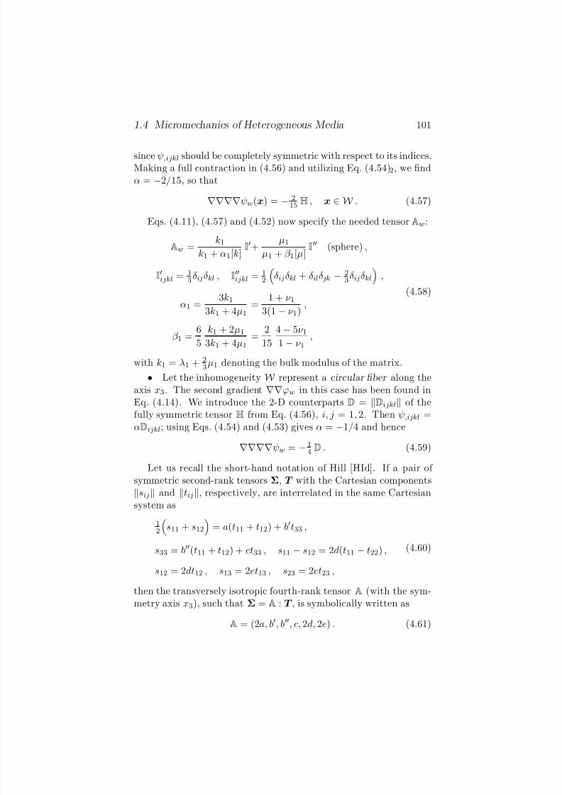
8/8/2019 Elementary Micro Mechanics of Heterogeneous Media
http://slidepdf.com/reader/full/elementary-micro-mechanics-of-heterogeneous-media 105/166
1.4 Micromechanics of Heterogeneous Media 101
since ψ,ijkl should be completely symmetric with respect to its indices.Making a full contraction in (4.56) and utilizing Eq. (4.54)2, we findα = −2/15, so that
ψw(x) = − 215 H , x ∈ W . (4.57)
Eqs. (4.11), (4.57) and (4.52) now specify the needed tensor Aw:
Aw =k1
k1 + α1[k]I+
µ1
µ1 + β 1[µ]I (sphere) ,
I
ijkl =13 δijδkl , I
ijkl =12 δijδkl + δilδ jk −
23 δijδkl ,
α1 =3k1
3k1 + 4µ1=
1 + ν 13(1 − ν 1)
,
β 1 =6
5
k1 + 2µ1
3k1 + 4µ1=
2
15
4 − 5ν 11 − ν 1
,
(4.58)
with k1 = λ1 + 23 µ1 denoting the bulk modulus of the matrix.
• Let the inhomogeneity W represent a circular fiber along theaxis x3. The second gradient ϕw in this case has been found inEq. (4.14). We introduce the 2-D counterparts D = Dijkl of the
fully symmetric tensorH
from Eq. (4.56), i, j = 1, 2. Then ψ,ijkl =αDijkl; using Eqs. (4.54) and (4.53) gives α = −1/4 and hence
ψw = −14 D . (4.59)
Let us recall the short-hand notation of Hill [HId]. If a pair of symmetric second-rank tensors Σ, T with the Cartesian componentssij and tij, respectively, are interrelated in the same Cartesiansystem as
12
s11 + s12
= a(t11 + t12) + bt33 ,
s33 = b(t11 + t12) + ct33 , s11
−s12 = 2d(t11
−t22) ,
s12 = 2dt12 , s13 = 2et13 , s23 = 2et23 ,
(4.60)
then the transversely isotropic fourth-rank tensor A (with the sym-metry axis x3), such that Σ = A : T , is symbolically written as
A = (2a, b, b, c, 2d, 2e) . (4.61)
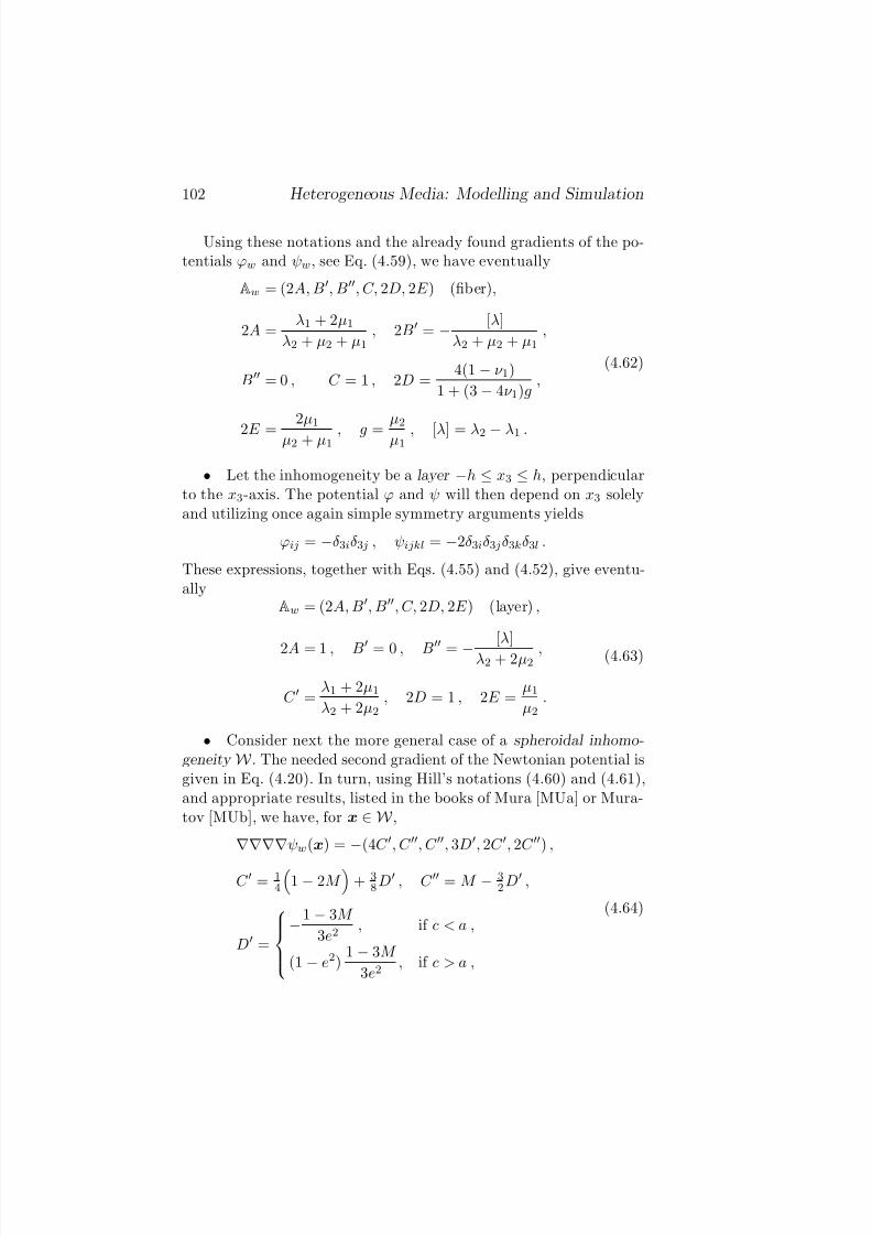
8/8/2019 Elementary Micro Mechanics of Heterogeneous Media
http://slidepdf.com/reader/full/elementary-micro-mechanics-of-heterogeneous-media 106/166
102 Heterogeneous Media: Modelling and Simulation
Using these notations and the already found gradients of the po-tentials ϕw and ψw, see Eq. (4.59), we have eventually
Aw = (2A, B, B, C, 2D, 2E ) (fiber),
2A =λ1 + 2µ1
λ2 + µ2 + µ1, 2B = − [λ]
λ2 + µ2 + µ1,
B = 0 , C = 1 , 2D =4(1 − ν 1)
1 + (3 − 4ν 1)g,
2E =
2µ1
µ2 + µ1 , g =
µ2
µ1 , [λ] = λ2 − λ1 .
(4.62)
• Let the inhomogeneity be a layer −h ≤ x3 ≤ h, perpendicularto the x3-axis. The potential ϕ and ψ will then depend on x3 solelyand utilizing once again simple symmetry arguments yields
ϕij = −δ3iδ3 j , ψijkl = −2δ3iδ3 jδ3kδ3l .
These expressions, together with Eqs. (4.55) and (4.52), give eventu-ally
Aw = (2A, B, B, C, 2D, 2E ) (layer) ,
2A = 1 , B
= 0 , B
= −[λ]
λ2 + 2µ2 ,
C =λ1 + 2µ1
λ2 + 2µ2, 2D = 1 , 2E =
µ1
µ2.
(4.63)
• Consider next the more general case of a spheroidal inhomo-geneity W . The needed second gradient of the Newtonian potential isgiven in Eq. (4.20). In turn, using Hill’s notations (4.60) and (4.61),and appropriate results, listed in the books of Mura [MUa] or Mura-tov [MUb], we have, for x ∈ W ,
ψw(x) = −(4C , C , C , 3D, 2C , 2C ) ,
C = 14
1 − 2M
+ 3
8 D , C = M − 32 D ,
D =
−1 − 3M
3e2, if c < a ,
(1 − e2)1 − 3M
3e2, if c > a ,
(4.64)
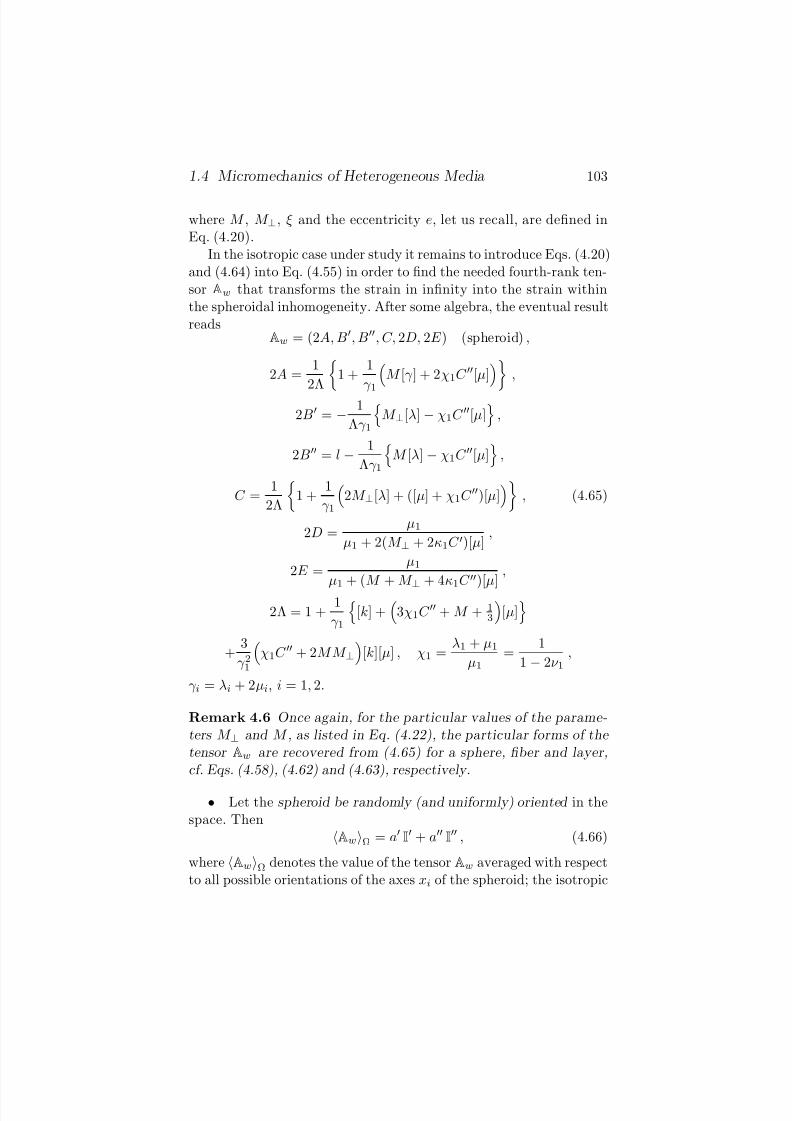
8/8/2019 Elementary Micro Mechanics of Heterogeneous Media
http://slidepdf.com/reader/full/elementary-micro-mechanics-of-heterogeneous-media 107/166
1.4 Micromechanics of Heterogeneous Media 103
where M , M ⊥, ξ and the eccentricity e, let us recall, are defined inEq. (4.20).
In the isotropic case under study it remains to introduce Eqs. (4.20)and (4.64) into Eq. (4.55) in order to find the needed fourth-rank ten-sor Aw that transforms the strain in infinity into the strain withinthe spheroidal inhomogeneity. After some algebra, the eventual resultreads
Aw = (2A, B, B, C, 2D, 2E ) (spheroid) ,
2A =1
2Λ 1 +1
γ 1 M [γ ] + 2χ1C [µ] ,
2B = − 1
Λγ 1
M ⊥[λ] − χ1C [µ]
,
2B = l − 1
Λγ 1
M [λ] − χ1C [µ]
,
C =1
2Λ
1 +
1
γ 1
2M ⊥[λ] + ([µ] + χ1C )[µ]
, (4.65)
2D =µ1
µ1 + 2(M ⊥ + 2κ1C )[µ],
2E =µ1
µ1 + (M + M ⊥ + 4κ1C )[µ],
2Λ = 1 +1
γ 1
[k] +
3χ1C + M + 1
3
[µ]
+
3
γ 21
χ1C + 2MM ⊥
[k][µ] , χ1 =
λ1 + µ1
µ1=
1
1 − 2ν 1,
γ i = λi + 2µi, i = 1, 2.
Remark 4.6 Once again, for the particular values of the parame-ters M ⊥ and M , as listed in Eq. (4.22), the particular forms of the tensor Aw are recovered from (4.65) for a sphere, fiber and layer,cf. Eqs. (4.58), (4.62) and (4.63), respectively.
• Let the spheroid be randomly (and uniformly) oriented in thespace. Then
AwΩ = a I + a I , (4.66)
where AwΩ denotes the value of the tensor Aw averaged with respectto all possible orientations of the axes xi of the spheroid; the isotropic
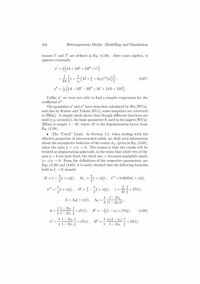
8/8/2019 Elementary Micro Mechanics of Heterogeneous Media
http://slidepdf.com/reader/full/elementary-micro-mechanics-of-heterogeneous-media 108/166
104 Heterogeneous Media: Modelling and Simulation
tensors I and I are defined in Eq. (4.58). After some algebra, it
appears eventually
a = 13
4A + 2B + 2B + C
=
1
2Λ
1 +
1
γ 1
M + 1
3 + 3χ1C [µ]
,
a = 115
2A − 2B − 2B + 2C + 12D + 12E
.
(4.67)
Unlike a
, we were not able to find a simpler expression for thecoefficient a.The quantities a and a have been first calculated by Wu [WUa],
and also by Kuster and Toksoz [KUc], some misprints are correctedin [BEm]. A simple check shows that though different functions areused (e.g. arcsinh ξ), the basic parameter θ, used in the papers [WUa],[BEm] is simply 1 − M , where M is the depolarization factor fromEq. (4.20).
• The “Crack” Limit. In Section 1.5, when dealing with theeffective properties of microcracked solids, we shall need informationabout the asymptotic behavior of the tensor Aw, given in Eq. (4.65),
when the ratio ξ = c/a → 0. The reason is that the cracks will betreated as degenerating spheroids, in the sense that while two of theaxes a = b are kept fixed, the third one, c, becomes negligibly small,i.e. c/a → 0. From the definitions of the respective parameters, seeEqs. (4.20) and (4.65), it is easily checked that the following formulaehold as ξ → 0, namely,
M = 1 − π
2ξ + O(ξ) , M ⊥ =
π
4ξ + O(ξ) , C = 0.0625πξ + O(ξ) ,
C =π
4ξ + O(ξ) , D = 2
3 − π
2ξ + O(ξ) , γ =
2
3π
1
ξ+ O(1) ,
Λ = Λ0ξ + O(ξ) , Λ0 = π8 1 − 2ν 1(1 − 2ν 1)2 ,
A =1
4
1 − 2ν 11 − 2ν 1
1
ξ+ O(1) , B = −1
4 (1 − ν 1) + O(ξ) , (4.68)
C =4
π
1 − 2ν 11 − 2ν 1
1
ξ+ O(1) , B =
4
π
ν 1(1 − ν 1)
1 − 2ν 1
1
ξ+ O(1) ,
8/8/2019 Elementary Micro Mechanics of Heterogeneous Media
http://slidepdf.com/reader/full/elementary-micro-mechanics-of-heterogeneous-media 109/166
1.5 Micromechanics of Heterogeneous Media 105
D = 12 + πξ
1 − 0.0125
1 − ν 1
+ O(ξ) , E =
2
π
1 − ν 12 − ν 1
1
ξ+ O(1) ,
a = 13 (4A + 2B + 2B + C ) =
4
3π
1 − ν 211 − 2ν 1
1
ξ+ O(1) ,
a = 115 (2A − 2B − 2B + 2C + 12D + 12E )
=8
15π
(1 − 2ν 1)(5 − ν 1)
2 − ν 1
1
ξ+ O(1) .
1.5 One-Particle Approximations
For simplicity, we shall consider the so-called particulate media , inwhich one of the constituents, called matrix , is connected. Through-out the latter particles of a second constituent (filler ), with a well-defined, in general, shapes are distributed. The properties of thematrix and of the filler are denoted, similarly to the previous section,by ‘1’ and ‘2’, respectively, so that, e.g. κ1 and κ2 are the appropriateconductivities, etc. Such a material is called also a dispersion (to be
thus distinguished from the case of suspension, when the particles areimmersed into a liquid and hence their relative positions are not fixeddue to the flow—a fact that tremendously complicates any theoreticalstudy).
Our aim here will be to demonstrate how various “repetitions”(to cite again Maxwell [MAj, Section 314]) of the single-inclusionsolutions of Section 1.1.3.3 can be systematically utilized in orderto derive the basic and most widely used approximate models forpredicting the effective properties of particulate media.
The basic idea is to invoke formulae like (2.41) that interconnectthe effective properties with the appropriate concentration factors, as
introduced in Sections 1.2.6—1.2.8. The latter are in turn approxi-mated by the appropriate solutions of the single-inclusion problem.Two natural possibilities are then opened. They can be summa-
rized as follows:
(i) Each inclusion is treated as single, immersed into a homoge-neous medium. The latter, as a consequence of the presence
8/8/2019 Elementary Micro Mechanics of Heterogeneous Media
http://slidepdf.com/reader/full/elementary-micro-mechanics-of-heterogeneous-media 110/166
106 Heterogeneous Media: Modelling and Simulation
of the host of other inclusions, possesses the unknown effective properties (the effective medium idea).
(ii) Each inclusion is again treated as single, but now immersed intothe matrix. The presence of the rest of inclusions is accountedfor by imaging that the inclusion is subjected to a certain ex-ternal field that differs from the applied macroscopic one (theeffective field idea).
We shall consider below some of the simplest implementations of
the assumptions (i) and (ii), within the frame of the static behavior of heterogeneous media. Their application and generalization for wavepropagation problems in such media are discussed and treated indetail in Chapter 3 of this volume.
1.5.1 Dilute Filler Fraction—Scalar Conductivity
Let us start with the simplest case, when there is no need either tomodify the medium’s properties or to change the applied field.
Namely, let the dispersion contain identical particles, of a fixedshape W , aligned throughout the matrix. We assume that the dis-persion is dilute , in the sense that the volume fraction, φ2, of the
particles is small, φ2 1, and hence their mutual influence can beneglected. Each particle can be thus imagined as single, immersedinto an unbounded matrix, and the “concentration factor” A2 is sim-ply the single-inhomogeneity tensor Aw(κ1, κ2), defined in Eq. (4.10).Thus, as it follows from (2.41),
K ∗ = κ1I + φ2[κ]Aw(κ1, κ2) + O (φ2) (5.1)
—both constituents are assumed isotropic but, due to the alignmentand nonspherical, in general, shape of the particles, the effective ten-sor K ∗ may be anisotropic. As underlined in (5.1), the formula iscorrect to the order O (φ2) only, providing however in this case an ex-act expression (since the particle interactions are totally neglected).To get the successive terms of order φ2
2 and higher, these interactionsshould be somehow accounted for. But, naturally, all schemes con-sidered below, that try to incorporate the interactions, agree in thedilute limit. More precisely, they all reproduce the formula (5.1) inthis case.
8/8/2019 Elementary Micro Mechanics of Heterogeneous Media
http://slidepdf.com/reader/full/elementary-micro-mechanics-of-heterogeneous-media 111/166
1.5 Micromechanics of Heterogeneous Media 107
Remark 5.1 Note that the approximation (5.1) has been used inmany of the earlier works on conductivity of two-phase media also inthe non-dilute case, see [REb] for some references. Perhaps its origincan be traced back to Laplace himself: According to Lorentz’ [LOb,Section 123], considering the connection between the density, ρ, of a transparent solid and its refraction index, µ2, Laplace reached the formula
µ2 − 1
ρ= const . (5.2)
But µ2 is just the dielectric constant of the medium, as already
pointed out (see the footnote on page 10), and the density ρ is pro- portional to the volume fraction of the dielectric spheres containedin the medium. Then (5.2) can be interpreted, somewhat loosely of course, as the dilute approximation of the type (5.1) for the effective dielectric constant of a dispersion.
Remark 5.2 “Dilute” formulae like (5.1) can be derived for hetero-geneous media in different physical context (see, e.g. Section 1.5.7 below where the absorption problem is addressed). The so-obtainedresults will make sense, however, only if the solution of the appropri-ate single-inclusion problem exists and is finite, like the tensor Aw
in Eq. (5.1). There are, unfortunately, situations when this solu-tion does not exist (say, for the same absorption problem in 2-D, see again the same Section 1.5.7). Then the appropriate effective prop-erties have no representation of the type (5.1); nonanalytic functions,like ln φ2, may emerge for small φ2 1 instead.
Consider in more detail the most important particular cases of theformula (5.1).
• Assume the inhomogeneities are spheres . From Eqs. (4.13) and(5.1) it follows
κ∗
κ1= 1 + 3βφ2 + O(φ2) , β =
[κ]
κ1 + 2κ2, (5.3)
which, naturally enough, reproduces the dilute limit (1.20) of theMaxwell prescription for κ∗.
• Consider a fiber-reinforced material , in which inhomogeneiti-es are parallel circular cylinders (along the axis x3). The effective
8/8/2019 Elementary Micro Mechanics of Heterogeneous Media
http://slidepdf.com/reader/full/elementary-micro-mechanics-of-heterogeneous-media 112/166
108 Heterogeneous Media: Modelling and Simulation
conductivity tensor is transversely isotropic
K ∗ = κ∗11(e1e1 + e2e2) + κ∗33e3e3 , (5.4)
where
κ∗11 = κ∗22 = κ1
1 +
2[κ]
κ1 + κ2φ2
+ O(φ2) ,
κ∗33 = κ = φ1κ1 + φ2κ2 ,
(5.5)
see (5.1) and (4.15). The coefficients κ∗11 = κ∗22 represent the trans-
verse conductivity of the fiber-reinforced medium, for dilute fiberconcentration φ2 1, in the case when the applied temperaturegradient is perpendicular to fibers’ axes. The conductivity compo-nent κ∗33 along the x3-axis is exactly the arithmetic mean κ, whichexplains why the higher order correction O(φ2) is missing in the sec-ond formula of (5.5). The reason is that the temperature field inthe medium is just θ(x) ≡ G3x3, if the applied gradient is along thefibers, i.e. if G = G3e3—a situation already discussed in Remark 2.1,see Eq. (2.11).
• Consider a layered material that consists of laminae, perpen-dicular to the axis x3. The appropriate tensor Aw is given in (4.17),
so that Eq. (5.1) implies
κ∗11 = κ∗22 = κ1 + φ2[κ] + O(φ2) , κ∗33 = κ1 + φ2[κ]κ1
κ2+ O(φ2) .
However, for such an exceptionally simple internal constitution thefollowing exact formulae for the effective conductivities hold
κ∗11 = κ∗22 = κ , i.e. 1/κ∗ = 1/κ = φ1/κ1 + φ2/κ2 . (5.6)
The reason is that the temperature gradient remains constant withinthe volume
V , if G is along the laminae. If G is along the axis x3, i.e.
perpendicular to the laminae, the heat flux is constant within V ; inthis case the effective compliance k∗ = 1/κ∗ is the arithmetic meanof the constituents’ compliances, see Remark 2.2 and Eq. (2.18).
• Let the inhomogeneities be identical and isotropic spheroids,aligned along the x3-axis , with the semiaxes c and a, c = a = b.In this case the tensor Aw is given in Eq. (4.21), the medium is
8/8/2019 Elementary Micro Mechanics of Heterogeneous Media
http://slidepdf.com/reader/full/elementary-micro-mechanics-of-heterogeneous-media 113/166
1.5 Micromechanics of Heterogeneous Media 109
transversely isotropic, with symmetry axis x3, and its effective con-ductivity tensor K ∗ is
K ∗ = κ∗11(e1e1 + e2e2) + κ∗33e3e3 ,
κ∗11 = κ∗22 = κ1
1 + φ2
[κ]
κ1 + [κ]M ⊥
+ O(φ2) ,
κ∗33 = κ1
1 + φ2
[κ]
κ1 + [κ]M
+ O(φ2) .
(5.7)
For the particular values of the parameters M and M ⊥, as listed
in Eq. (4.22), the already given formulae (5.3), (5.5) and (5.6) forthe effective conductivities in the cases of spheres, fibers and layers,respectively, show up.
• Let the inhomogeneities be again identical, but randomly ori-ented and isotropic spheroids , with the semiaxes c and a. In thiscase the tensor Aw = AwΩ is given in Eq. (4.23), the medium ismacroscopically isotropic and its effective conductivity reads
κ∗
κ1= 1 +
[κ]
3κ1
2κ1
κ1 + [κ]M ⊥+
κ1
κ1 + [κ]M
φ2 + O(φ2) . (5.8)
The parameters M and M ⊥ depend on the eccentricity of the sphe-
roids, see Eq. (4.20).• Let the spheroids, again randomly oriented in the space, de-
generate into penny-shaped cracks . In this case κ2 = 0 and the termin the brackets in the right-hand side of (5.8) has the asymptotic
m =2
1 − M ⊥+
1
1 − M =
2
π
1
ξ+ O(ξ) , ξ = c/a → 0 , (5.9)
as it follows from Eq. (4.68). Eq. (5.8) now yields
κ∗
κ1= 1 − n 4
3 πa2cm = 1 − (na3) 43 π
c
am
= 1 − ε43 πξm + O(ξ) −→ξ→0 1 −
89 ε ,
(5.10)
in virtue of Eq. (5.9). Here n is number density of the spheroids(i.e. their number per unit volume), so that φ2 = nV , V = 4
3 πa2c isthe volume of the single spheroid, and
ε = na3 (5.11)
8/8/2019 Elementary Micro Mechanics of Heterogeneous Media
http://slidepdf.com/reader/full/elementary-micro-mechanics-of-heterogeneous-media 114/166
110 Heterogeneous Media: Modelling and Simulation
is the so-called crack density parameter —the counterpart of the vol-ume fraction of the inclusions in the case of cracked solids (as in-troduced and very often employed for such solids, see the survey of Kachanov [KAa]). Thus the effective conductivity of a solid, contain-ing a dilute population of randomly oriented penny-shaped cracks, is
κ∗
κ1= 1 − 8
9 ε + O(ε) , (5.12)
1.5.2 Dilute Filler Fraction—Elastic Case
In the elastic case and for a dilute particle concentration we have, asa consequence of Eq. (2.64),
L∗ = L1 + φ2[L] : Aw(L1,L2) + O(φ2) , (5.13)
where Aw is the fourth-rank tensor that comes out from the solutionof the elastic single inclusion problem, see Section 1.4.4.
Remark 5.3 Since the formula (5.13) is exact, the tensor
[L] : Aw(L1,L2)
possesses the needed “external” symmetry (2.65), whatever the shape of the inclusions W .Similarly to the previous subsection, consider the most interesting
particular cases of the formula (5.13).
• For an isotropic dispersion of spheres the tensor Aw is givenin Eq. (4.58) and hence
k∗
k1= 1 +
[k]
k1 + α1[k]φ2 + O(φ2) ,
µ∗
µ1
= 1 +[µ]
µ1 + β 1[µ]
φ2 + O(φ2) ;
(5.14)
α1 and β 1 depend on the Poisson ratio, ν 1, of the matrix, see thesame Eq. (4.58).
Remark 5.4 The formulae (5.14) have been first derived by Brugge-man [BRg]. (Though, as pointed out in [ESa], his result for the shear
8/8/2019 Elementary Micro Mechanics of Heterogeneous Media
http://slidepdf.com/reader/full/elementary-micro-mechanics-of-heterogeneous-media 115/166
8/8/2019 Elementary Micro Mechanics of Heterogeneous Media
http://slidepdf.com/reader/full/elementary-micro-mechanics-of-heterogeneous-media 116/166
112 Heterogeneous Media: Modelling and Simulation
—the counterpart of the Einstein’ formula, giving the viscosity of adilute bubbly liquid in the Stokesian approximation. This result is attributed to Taylor [TAd].
• Let the inhomogeneities be identical but randomly orientedspheroids . Then the material is macroscopically isotropic and (5.13)implies
k∗
k1= 1 +
[k]
k1aφ2 + O(φ2) ,
µ∗
µ1= 1 +
[µ]
µ1aφ2 + O(φ2) , (5.16)
with the coefficients a and a, given in Eq. (4.67).
• Let κ2 = 0 and the spheroids, again randomly oriented in thespace, degenerate into penny-shaped cracks . Using the asymptotic(4.68) of the coefficients a and a in the “crack” limit, together withEq. (5.16), one gets
k∗
k1= 1 − 16
9
1 − ν 211 − 2ν 1
ε + O(ε) ,
µ∗
µ1= 1 − 32
45
(1 − ν 1)(5 − ν 1)
2 − ν 1ε + O(ε) ,
(5.17)
having recalled the definition (5.11) of the crack density parameter ε.The formulae (5.17) have been independently proposed by Bristow
[BRc] and Walsh [WAa].
Remark 5.7 Treating the crack as a vacuous oblate spheroid of ec-centricity approaching zero is very convenient. To the best of the author’s knowledge it was first employed by Willis [WIb]. The reasonis that it allows one to derive straightforwardly the needed formula for a microcracked solid, passing (with a due care) to the appropri-ate limits in the general formulae, concerning ellipsoidal inclusions.The usefulness of this idea was already demonstrated in deriving Eqs. (5.12) and (5.17). In the elastic context an alternative deriva-tions employ specific notions and results from fracture mechanics, like stress-concentration factors, energy release rate, etc. Such a deriva-tion, employed in particular in the original Bristow’s paper [BRc], or in [BEc], is often difficult for a “fracture outsider” to follow.
8/8/2019 Elementary Micro Mechanics of Heterogeneous Media
http://slidepdf.com/reader/full/elementary-micro-mechanics-of-heterogeneous-media 117/166
1.5 Micromechanics of Heterogeneous Media 113
1.5.3 Self-Consistent Scheme
When the volume fraction becomes higher (say, φ2 ≥ 0.05) it is notalready realistic to imagine the inclusions isolated. Somehow theirmutual interactions should be accounted for. The simplest way todo this, at least qualitatively, is the application of the self-consistentidea that appeared, in a certain form, already in the Clausius deriva-tion [CLa] of the Maxwell formula, mentioned in Section 1.1. Nextit showed up as a very useful and natural tool in solid-state physicsand, more specifically, in the wave mechanics of atoms, as originatedby Hartree [HAb]. In the context of effective properties of heteroge-
neous media the self-consistent approach seems to be first employedby Bruggeman [BRf], [BRg], see also [FRd], [LAb]. In the quest of the elastic constants of polycrystals, the method is attributed to Her-shey [HEb] and Kroner [KRd]. (In Section 1.6 below we shall presentin more details the reasoning and some results of these two authors.)
1.5.3.1 The Basic Idea
The basic idea of the self-consistent scheme (SCS) is to treat eachparticle again as isolated, but immersed into a matrix possessing theunknown effective properties of the composite. This means that weshould replace Eq. (5.1) and its elastic counterpart (5.13) by the
equationsK ∗ = κ1I + φ2[κ]Aw(κ1,K ∗) (scalar case) ,
L∗ = L1 + φ2[L] : Aw(L1,L∗) (elastic case) .
(5.18)
In each particular case, Eqs. (5.18) will yield appropriate algebraicequations for the unknown effective properties of the composite.
To demonstrate this, consider the simplest example when the in-clusions are spheres. In the scalar context, Eq. (4.13) is to be intro-duced into the first equation of (5.18):
κ∗
κ1= 1 +
[κ]
κ1
3κ∗
κ2 + 2κ∗φ2 (5.19)
which represents, obviously, a quadratic equation with respect to theeffective conductivity.
Eq. (5.19) was proposed by Bruggeman [BRf], see also [LAb], inthe equivalent form
φ1κ1 − κ∗
κ1 + 2κ∗+ φ2
κ2 − κ∗
κ2 + 2κ∗= 0 . (5.20)
8/8/2019 Elementary Micro Mechanics of Heterogeneous Media
http://slidepdf.com/reader/full/elementary-micro-mechanics-of-heterogeneous-media 118/166
114 Heterogeneous Media: Modelling and Simulation
Note the symmetry of the latter with respect to the constituents’characteristics, that is under the simultaneous interchange κ1 ↔ κ2
and φ1 ↔ φ2. That is why Eq. (5.19) is often called symmetric effective medium approximation (EMA), or First Bruggeman’s sym-metric EMA—a term, introduced by Landauer [LAc]. Thus eachphase should be treated on the same footing, as pointed out by Davies[DAb]; in the above reasoning however one of the phase was imaginedcontinuous, and the second in the form of distributed inclusions; thisalready implies an inherent logical inconsistency of the SCS. Morefundamental, however, is the inconsistency, very clearly exposed by
Hashin [HAi], namely, the violation of the basic MMM principle, for-mulated in Section 1.2.1. The point is that a single sphere in thedispersion is the basic micro element and as such it can only “see”the other spheres (micro-elements) around, but not the mini-element(the homogenized medium) as a whole, whose properties result fromaveraging over the multitude of all the micro-elements within it. Or,as Hashin put it: SCS assumes that a tree sees the forest—but a tree sees only other trees.
The foregoing does not imply however that the SCS is useless andshould be rejected. It simply suggests that if the scheme is realistic,the appropriate two-phase geometries cannot resemble a dispersion
of equi-sized spheres. That this is indeed the case follows from animportant result of Milton [MIe]. It states that the SCS (more pre-cisely, Eq. (5.19) or Eq. (5.20)) is a realizable approximation in thesense that there exists a special, ingeniously devised, internal geom-etry of a two-phase medium whose effective elastic moduli coincideexactly with the SCS predictions of Eq. (5.19). The reader is referredto the original Milton’s work since the details and proofs cannot beelementary summarized. We can only add that, like Hashin’s assem-blage (Section 1.3.4), the “SCS-geometry” of Milton is of fractal-type(self-similar in all length-scales, that is), comprising inclusions of allpossible sizes, from finite down to infinitesimally small. Due to theforegoing remarks, it is a little wonder that such a geometry hasnothing in common with equi-sized particles like spheres, distributedthroughout a matrix.
Remark 5.8 The choice of the basic element, to be inserted into the effective medium, is not unique in the SC scheme. In the foregoing,the simplest possibility was chosen, when this is just the filler parti-
8/8/2019 Elementary Micro Mechanics of Heterogeneous Media
http://slidepdf.com/reader/full/elementary-micro-mechanics-of-heterogeneous-media 119/166
1.5 Micromechanics of Heterogeneous Media 115
cle. This is however not the only choice; more complicated elements can be devised as well. For example one can take a “composite”sphere, with a kernel of phase ‘1’, coated by a layer of phase ‘2’,as first suggested by Kerner [KEa]. A detailed and critical analysis of such a SCS modification can be found in [HAg]; for generaliza-tions in the elastic case, see [CHe] or [CHd, Chapter 2.3]. This kindof modification of the self-consistent method are usually referred toas Generalized Self-Consistent-Schemes (GSCS), but their discussiongoes beyond the frame of the present survey. It should be only notedthat without detailed morphological information, no theoretical ar-
guments can be given for any specific choice of a basic element in a binary medium. (The “composite” sphere was used in [CHe] or [CHd]because the appropriate model provided better agreement with cer-tain precise experimental data; though no guarantee exists whether it will work equally well for other sets of experiments.) For polycrys-tals, however, the basic element is naturally predetermined from the very internal structure—this is just the single grain (see Section 1.6).The latter perhaps explains why the SCS provides as a rule more accurate predictions for the effective properties of polycrystals thanof particulate media.
Note finally that the self-consistent method can be employed in anobvious manner to multiphase media as well. However, its predictionswill possess the needed symmetry (2.65) only when the dispersedinclusions are aligned and of similar shape, see the paper [BEe] fordetails, examples and comments on this important fact.
1.5.3.2 An Alternative Derivation
Eq. (5.20) can be also recast as
κ(x) − κ∗
κ(x) + 2κ∗= 0 , (5.21)
where the overbar indicates, let us recall, averaging over the RVE,and κ(x) is the function that takes the values κ1 or κ2 depending onwhether x lies in the constituent ‘1’ or ‘2’, respectively. Eq. (5.21) hasa simple and clear interpretation. Namely, imagine that the RVE, V ,is filled with spherical particles, whose sizes vary from finite down toinfinitesimal. The spheres have conductivity κ1 or κ2. Imagine each
8/8/2019 Elementary Micro Mechanics of Heterogeneous Media
http://slidepdf.com/reader/full/elementary-micro-mechanics-of-heterogeneous-media 120/166
116 Heterogeneous Media: Modelling and Simulation
sphere lying in a homogeneous medium with the effective conductivi-ties κ∗; at infinity the prescribed temperature gradient G is imposed.The deviation from this gradient within the sphere, due to the factthat its properties differ from those of the surrounding material, is just
κ(x) − κ∗
κ(x) + 2κ∗G , (5.22)
cf. Eqs. (1.14) and (1.15). (In the electrostatic context, the lattervalue is proportional to the so-called polarization of the sphere.)Since the volume
V is considered as macroscopically homogeneous,
we should have, accordingly, no macroscopical polarization. Themean value of the “local” polarizations (5.22) should then vanish,as claimed in Eqs. (5.20) and (5.21).
The above reasoning can be interpreted as well in the followingmanner, that represents a modification of the original Maxwell argu-ments of Section 1.1.3.3. Cut again a big sphere of the radius A (the“Maxwell sphere”) from the heterogeneous medium and immerse itinto unbounded homogeneous host material whose conductivity κ+
will be appropriately chosen (or, so to say after Berryman [BEm],“tuned”). “Sit down” at the point M far away, i.e. at the distance Rfrom the center of the sphere, R A. Let the temperature field G ·xbe applied at infinity. Each piece of the phases ‘1’ or ‘2’, located inthe vicinity of x, will create at the point M the disturbance
a3
R3
κ(x) − κ+
κ(x) + 2κ+G , (5.23)
—since we are far from the piece under consideration, it can be takenas spherical with a radius a. Averaging (5.23) over the big heteroge-neous sphere will give a quantity, proportional to
κ(x) − κ+
κ(x) + 2κ+. (5.24)
Comparing (5.24) with (5.21) shows that if we “tune” the host mediumso that κ+ = κ∗, the presence of the heterogeneous sphere will notbe “felt” at the point M ; in other words this sphere will become“transparent” for us.
The above arguments represent a “static” (and scalar) implemen-tation of Berryman’s idea [BEm]: this author dealt with the long-wave length limit for a harmonic wave, scattered by the “Maxwell
8/8/2019 Elementary Micro Mechanics of Heterogeneous Media
http://slidepdf.com/reader/full/elementary-micro-mechanics-of-heterogeneous-media 121/166
8/8/2019 Elementary Micro Mechanics of Heterogeneous Media
http://slidepdf.com/reader/full/elementary-micro-mechanics-of-heterogeneous-media 122/166
118 Heterogeneous Media: Modelling and Simulation
It is noted that the percolation phenomena are very importantin solid state physics, in general, and in many of its applications.The appropriate discussion goes however far beyond the scope of thepresent work (see the survey [LAc] or [KIa] for basic ideas, resultsand classical references).
Remark 5.10 In the literature the presence of a percolation thresh-old is sometimes considered as a virtue of an approximate model,while its lack (in the differential scheme below, for example) is viewedas a drawback (or vice versa, depending on author’s taste). It should
be noted that the threshold’s presence (or lack) has nothing in com-mon with the validity of the model. It only informs us that for the geometry that realizes the model (like Milton’ SCS-geometry), there is (or there is not) a threshold. Hence this is a conclusion concern-ing above all a specific two-phase geometry, but not a model or its applicability.
1.5.3.4 Some Particular Cases
Consider now, for illustration, several particular cases of the SCSequations (5.18).
• For randomly oriented and isotropic spheroids , in the scalarconductivity case,
κ∗
κ1= 1 +
[κ]
3κ1
2κ∗
κ∗ + (κ2 − κ∗)M ⊥+
κ∗
κ∗ + (κ2 − κ∗)M
φ2 , (5.26)
cf. Eqs. (4.21) and (5.18). When the spheroids are spheres, M =M ⊥ = 1
3 , and (5.26) reproduces (5.19).
• Let κ2 = 0, and the spheroids degenerate into penny-shapedcracks. The effective conductivity κ∗ is then eliminated from theright-hand side of Eq. (5.26) and Eq. (5.12) is recovered, but with-
out the correction term O(ε), cf. Eq. (5.9). Hence the self-consistentscheme predicts the linear dependence
κ∗
κ1= 1 − 8
9 ε (5.27)
of κ∗ upon the crack density parameter.
8/8/2019 Elementary Micro Mechanics of Heterogeneous Media
http://slidepdf.com/reader/full/elementary-micro-mechanics-of-heterogeneous-media 123/166
1.5 Micromechanics of Heterogeneous Media 119
The results in the elastic case are obtained in a fully similar way,and we shall only list some of the basic ones.
• For an isotropic elastic dispersion of spheres , the self-consistentscheme yields
k∗ = k1 + k∗k2 − k1
k∗ + α∗(k2 − k∗)φ2 ,
µ∗ = µ1 + µ∗µ2 − µ1
µ∗ + β ∗(µ2 − µ∗)φ2 ,
α∗ = 3k∗
3k∗ + 4µ∗, β ∗ = 6
5k∗
+ 2µ∗
3k∗ + 2µ∗,
(5.28)
see Eqs. (5.18) and (4.58). This is an algebraic system with respectto the unknown effective moduli k∗ and µ∗ which allows a convenientnumerical solution (by a straightforward iterative procedure).
The system (5.28) is usually attributed to Budiansky [BUa] andHill [HIe], see also [WUa]. (These authors were apparently not awareof the earlier Skorohod’s paper [SKa], where the same classical self-consistent reasoning was employed to derive (5.28).)
Very simple closed form solutions (5.28) can be found, if ν 1 = ν 2 =0.2. Then, as pointed out by Budiansky [BUa], the Poisson ratio of the medium is also 0.2, α∗ = β ∗ ≡ 0.5.
Other simple solutions exist if the Poisson ratio of the matrix isagain ν 1 = 0.2, but the inclusions are rigid or represent voids. Inparticular, for spherical voids in a matrix of Poisson ratio ν 1 = 0.2,the solution of (5.28) is extremely simple
κ∗
κ1=
µ∗
µ1= 1 − 2φ2 (k2 = µ2 = ∞) ,
κ∗
κ1=
µ∗
µ1=
1
1 − 2φ2(k2 = µ2 = 0) ,
(5.29)
and hence ν ∗ ≡ 0.2 in both cases.The foregoing facts suggest that the value 0.2 of the Poisson ratio
is something special in the “one-particle” models of particulate me-dia.14 A certain explanation can be sought perhaps in the fact that
14It was Hashin [HAc] who first pointed out the “curious” fact that ν ∗ ≡ 0.2 ina dilute dispersion of rigid spheres in a matrix for which ν 1 = 0.2.
8/8/2019 Elementary Micro Mechanics of Heterogeneous Media
http://slidepdf.com/reader/full/elementary-micro-mechanics-of-heterogeneous-media 124/166
120 Heterogeneous Media: Modelling and Simulation
at ν 1 = 0.2 the concentration factor for a single spherical inclusion—the tensor Aw, as given in Eq. (4.58), is proportional to the unitfourth-rank tensor I.
Eq. (5.29) means that for a dispersion of spheres, in a matrix withν 1 = 0.2, the percolation threshold, as predicted by SCS, is φp
2 = 0.5.At sphere fractions, higher than 0.5, the solid either become rigid orcannot sustain load. Again, this fact is neither a merit or a fault of the SCS, but just a property of the special Milton’s SCS-geometrythat “lies” behind the scheme.
Another simple solution of (5.28) emerges for the Hill medium,
when the shear moduli of the phases coincide, µ1 = µ2 = µ. Then,from the first equation, one has
k∗ − k1
k2 − k1= φ2
3k∗ + 4µ
3k2 + 4µ. (5.30)
which reproduces the Hill formula (3.66). Hence the SCS gives theexact value of the effective bulk modulus in the case of sphericalparticles. (Recall, however, that the Hill results (5.30) holds for anarbitrary two-phase geometry, which is macroscopically isotropic.)
• For an isotropic elastic solid, containing randomly oriented penny-shaped cracks , we get formally the same system (5.17), withthe only difference that the Poisson ratio of the matrix, ν 1, is replacedby this ratio of the composite medium, ν ∗:
k∗
k1= 1 − 16
9
1 − ν ∗2
1 − 2ν ∗ε ,
µ∗
µ1= 1 − 32
45
(1 − ν ∗)(5 − ν ∗)
2 − ν ∗ε .
(5.31)
This is exactly the self-consistent system of Budiansky and O’Connell[Bub] for the effective moduli of a microcracked solid (cf. their Eqs.(36) and (44)).
1.5.4 The Differential Scheme
The differential scheme (DS) is a kind of an “infinitesimal” imple-mentation of the self-consistent idea. It was initiated by Bruggeman[BRf], [BRg] and used in fifties for media containing rigid particles(by Brinkman [BRb] for the viscosity of a fluid suspension, and by
8/8/2019 Elementary Micro Mechanics of Heterogeneous Media
http://slidepdf.com/reader/full/elementary-micro-mechanics-of-heterogeneous-media 125/166
1.5 Micromechanics of Heterogeneous Media 121
Roscoe [ROa] in the elastic case). More recently it was elaborated byMcLaughlin [MCb], Norris [NOa], Zimmerman [ZIc] et al. A detaileddiscussion can be found in the survey [CLb].
1.5.4.1 The Basic Idea
Imagine the small concentration δΓ of particles is added to an initiallyhomogeneous medium. Replace mentally the so obtained mixture bya homogeneous medium of the effective conductivity K ∗ = K ∗(δΓ).In the latter a new concentration δΓ of particles is inserted; thenew medium again is replaced by a homogeneous one of conductiv-
ity K ∗(2δΓ), and so forth. As a result, the effective conductivitywill be a certain function of the total amount Γ of inserted particles,K ∗ = K ∗(Γ). Since at each step a small concentration of particles isadded, δΓ 1, the dilute approximation (5.1) applies
K ∗(Γ + δΓ) = K ∗(Γ) + δΓ (κ2I −K ∗(Γ)) ·Aw(K ∗(Γ), κ2) .
In the limit δΓ → 0, this yields the differential equation
dK ∗
dΓ= (κ2I −K ∗(Γ)) ·Aw(K ∗(Γ), κ2) (5.32)
for the unknown function K ∗ = K ∗(Γ), which should be solved to-
gether with the natural initial condition
K ∗(0) = κ1I .
The reasoning in the elastic case is fully similar, and will be omit-ted.
It is very important to point out, after McLaughlin [MCb], thatthe total concentration Γ of particles, introduced into the matrix,does not coincide with the volume concentration φ2 of the secondphase. The reason is that when adding a new portion δΓ of particles,some of them will “fall” within the region, occupied by the previouslydeposited ones. Only the part φ1δΓ, that “falls” within the matrix,will increase φ2. Thus, in the limit δΓ → 0 again,
dφ2 = (1 − φ2) dΓ or Γ = − ln(1 − φ2) , (5.33)
because, obviously, Γ = 0 at φ2 = 0. From (5.33) it follows that
Γ = φ2 + 12 φ2
2 − · · · ,
8/8/2019 Elementary Micro Mechanics of Heterogeneous Media
http://slidepdf.com/reader/full/elementary-micro-mechanics-of-heterogeneous-media 126/166
122 Heterogeneous Media: Modelling and Simulation
which means that Γ ≈ φ2 for φ2 1. Hence only for small values of φ2 one can choose Γ = φ2.
Remark 5.11 In some of the earlier papers [HEa], [ZIb], the differ-ential scheme was applied without distinguishing between the quan-tity Γ and the fraction φ2. One of the motivation was Mackenzie’s treatment of a porous solid [MAa], in which a new single pore is addedat the center of a sphere, cut from the homogenized medium, and sub- jected to hydrostatic pressure. As just pointed out, taking Γ = φ2
is safe only in the dilute case; for higher values of φ2 the deviations from the differential scheme’s predictions is already considerable.
Obviously, the phases do not enter symmetrically in the Eqs. (5.32)and (5.33), unlike the self-consistent scheme. On the other hand againthe effective medium surrounding of the inclusion is imagined at eachstep of the DS procedure. That is why the DS is often called, afterLandauer [LAc], the Second Bruggeman’s unsymmetrical Effective Medium Approximation. Also the term iterated dilute limit approx-imation is sometimes used, which reflects well the reasoning that hasled us to the formulae (5.32) and (5.33).
The differential scheme, similarly to the self-consistent one, is a re-alizable approximation in the sense that there exist special two-phasemedia whose effective behavior coincides exactly with the predictionsof the scheme. This important fact was first demonstrated by Norriset al. [NOa], [NOb], [NOc], see also [AVa].
1.5.4.2 Some Particular Cases
Consider now in more detail the system (5.32) and (5.33) in severalparticular cases.
• For spherical inclusions in the scalar conductivity context thetensor K ∗ = κ∗I is isotropic and Aw is given in (4.13). Eq. (5.32)then becomes
df
dφ2
=3(α − f (φ2))f (φ2)
(1 − φ2)(α + 2f (φ2))
, κ∗/κ1 = f (φ2) , (5.34)
α = κ2/κ1. Similarly to the self-consistent scheme, Eq. (5.34) allowssimple solutions
κ∗
κ1=
1
(1 − φ2)3, if κ2/κ1 = ∞ ,
(1 − φ2)3/2 , if κ2/κ1 = 0 ,
(5.35)
8/8/2019 Elementary Micro Mechanics of Heterogeneous Media
http://slidepdf.com/reader/full/elementary-micro-mechanics-of-heterogeneous-media 127/166
1.5 Micromechanics of Heterogeneous Media 123
in the two limiting cases of ideally conducting particles (κ2/κ1 = ∞)or non-conducting particles (κ2/κ1 = 0), respectively. Hence, thereis no percolation in the differential scheme—the values of κ∗ remainfinite and positive for all φ2 ∈ (0, 1).
• For spherical inclusions in the elastic case the DS supplies thesystem
1
k∗dk∗
dφ2=
(3k∗ + 4µ∗)(k2 − k∗)
(1 − φ2)k∗(3k2 + 4µ∗),
1µ∗
dµ∗
dφ2= 5(3k
∗
+ 4µ∗
)(µ2 − µ∗
)(1 − φ2)(6µ∗(k∗ + 2µ∗) + (9k∗ + 8µ∗)µ∗)
,
(5.36)
coupled with the obvious initial conditions k(0) = k1, µ(0) = µ1.The system (5.36) was derived by McLaughlin [MCb] who showed, inparticular, that its solution meets the HS bounds.15
A detailed analysis of the system (5.36) was performed by Zim-merman [ZIc]. He observed that (5.36) is autonomous, with the pa-rameter Γ, see Eq. (5.33), playing the role of time. This suggeststo divide the equations of (5.36) and the result will be an explicit,though complicated, expression of φ2 through the ratio k∗/µ∗ (or
which is the same, through the effective Poisson ratio ν ∗
). Simplersolutions exist in the limiting cases of rigid and vacuous inclusions.The equation for ν ∗ that follows from (5.36) has in these cases theform
dν ∗
dΓ= F (ν 1)(1 − 5ν 1) .
Though the function F (ν 1) is different for rigid and vacuous inclu-sions, the presence of the multiplier 1 −5ν 1 in both cases assures thatν ∗ ≡ 0.2, if ν 1 = 0.2—something that is identical with the predictionsof the SCS. Moreover, the value 0.2 of the Poisson ratio is an attrac-tor or a fixed point, in the sense that the function ν ∗ = ν ∗(φ2) is
monotonically increasing, if ν ∗
(0) = ν 1 < 0.2, and monotonically de-creasing, if ν ∗(0) = ν 1 > 0.2. In both cases ν ∗(φ2) → 0.2 as φ2 → 1.The same attractor’s type behavior has been observed in the SCS bythe author [MAd].
15Once an approximate scheme is realizable, its predictions always satisfy theHS bounds, due to the optimality of the latter; see Section 1.3.3.
8/8/2019 Elementary Micro Mechanics of Heterogeneous Media
http://slidepdf.com/reader/full/elementary-micro-mechanics-of-heterogeneous-media 128/166
124 Heterogeneous Media: Modelling and Simulation
Remark 5.12 It is curious to understand whether the peculiarity of the value 0.2 for the Poisson ratio is something that indeed exists inreal heterogeneous solids, or it is a mathematical artifact producedby the models. This intriguing question explains the considerable interests in the last 15 years in studying the so-called Poisson ratio flow diagrams i.e. the effective Poisson coefficient as a function of the volume fraction φ2 of the inclusions. It turned out that if the inclusions are voids, the fixed points on such diagrams (like the above value 0.2) do exist, and this was demonstrated both analytically (see,e.g. [CHb] in 2-D) and numerically by a number of authors. Details,
discussion and many references can be found in the recent paper [CHf].
For rigid inclusions it seems as if there are no fixed points for the Poisson ratio, as numerical experiments suggest, see again [CHf].The apparent discrepancy between voids and rigid inclusions may be however a by-product of the numerical procedures, employed by the authors. After Zimmerman [ZId], one can point out that calculations for a medium with “vacuous pores” can be performed simply putting the elastic moduli κ2 = µ2 = 0 in the appropriate equations andnumerical schemes. But the analogous calculations for rigid inclusions are performed taking the moduli κ2, µ2 very large, but still finite.
One should be very careful, dealing with limit of moduli, tending both to zero and to infinity. The problem arises because, when taking either limit 0 or ∞, any references of the Poisson ratio may be lost. Infact, one can construct paths κ2, µ2 → 0 or ∞ in ( κ2, µ2)-space so thatthe Poisson ratio can have any value. For more details, concerning this subtle situation, the reader is referred to the original paper [Zid].
Another similarity with the SCS is the existence of the simple solu-tions of (5.36), when ν 1 = 0.2, for the two limiting types of inclusions,namely
k∗
k1=
µ∗
µ1= (1 − φ2)2 (voids) ,
k∗
k1=
µ∗
µ1=
1
(1 − φ2)2(rigid inclusions) ,
(5.37)
cf. Eq. (5.35).
Remark 5.13 Relations of the type (1 − φ2)m for the decrease of a certain effective property of a porous solid as a function of the
8/8/2019 Elementary Micro Mechanics of Heterogeneous Media
http://slidepdf.com/reader/full/elementary-micro-mechanics-of-heterogeneous-media 129/166
1.5 Micromechanics of Heterogeneous Media 125
void ratio φ2 are very popular and useful in some applications like micromechanics of microporous rocks. (In this context m is knownas the cementation exponent and its value supplies additional mi-crostructural information, see [SEa] for details and references.) They are often called Archie’s after the work [ARa]. The reappearance of the phenomenological Archie’s law within the DS, cf. (5.35) and(5.37), cannot be interpreted, however, as a kind of justification of the scheme or as an indication of its superiority as compared to other approximate theories. It means solely that the specific two-phase Norris’ microgeometry that “lies” behind the DS, exhibits Archie’s
type behavior of its effective conductivity and elasticity (for ν 1 = 0.2in the latter case).
Another particular case, in which the system (5.36) possesses avery simple solution, is when both the matrix and spheres are rigid.Then k1 = k2 = k∗ = ∞ and
µ∗
µ1=
1
(1 − φ2)5/2(5.38)
which reproduces the Einstein formula (1.21) in the dilute limit (re-calling once again the full mathematical analogy between an incom-
pressible elastic solid and a fluid in Stokesian approximation). Theformula (5.38) was proposed by Brinkman [BRb] for the viscosity of a fluid suspension, within his attempt of extending the Einstein for-mula (1.21) in nondilute case. To this end the author has utilizedliterally the same DS reasoning of Section 1.5.4.1.
We shall skip further study of the DS model and equations, re-ferring to the already cited papers of McLaughlin, Norris et al. andZimmerman. Also the application of the DS to the microcrackedsolids will not be discussed (in this case some care is needed, dueto the “degenerated” nature of the inclusions). Details and furtherreferences can be found in the Hashin paper [HAj], see also [HEa].
1.5.5 The Effective Field
Here again each particle is treated as single. However, we imagineit immersed now into a homogeneous medium possessing the prop-erties of the matrix. The influence of the rest of the particles isaccounted for through the assumption that the particle lies within
8/8/2019 Elementary Micro Mechanics of Heterogeneous Media
http://slidepdf.com/reader/full/elementary-micro-mechanics-of-heterogeneous-media 130/166
126 Heterogeneous Media: Modelling and Simulation
a certain external field—the effective field—that differs from the ap-plied macroscopic one. Similarly to the self-consistent scheme, thisis an old approach that goes back to the Mossotti cavity idea and tothe Lorenz-Lorentz local field, as we shall point out below.
1.5.5.1 The Basic Idea
We shall first implement the effective field idea again in the scalarcase. Let G∗ be the local (effective, or Lorenz-Lorentz’ in the dielec-tric context) field that acts on each particle; in this simplest versionit is assumed that G∗ is a constant.
Since each particle is lying as single in the field, it is natural alsoto assume that
θ1 = G∗ . (5.39)
As a matter of fact, this is the basic assumption of the simplestversion of the effective field method—it states that each particle un-dergoes an external field that coincides with the mean field in thematrix phase.
In turn, G∗ should depend linearly on the applied macroscopicgradient G = θ
G∗ = B ·G , (5.40)
with a certain second-rank tensor B. The latter is specified by means
of (5.39) and the first equation of (2.35):
G = θ = φ1 θ1 + φ2 θ2
= φ1G∗ + φ2Aw(κ1,K 2) ·G∗
= (φ1I + φ2Aw(κ1,K 2)) ·G∗ ;
(5.41)
we have used that θ2 = Aw(κ1,K 2) · G∗ since each particle istreated as single in the far-field G∗, according to the basic assump-tion. Hence
B = (φ1I + φ2Aw(κ1,K 2))−1 , (5.42)
which gives explicitly the tensor B that interconnects the appliedmacroscopic field and the resulting local one.
The concentration tensor can be easily found now by means of (5.41) and (5.42):
θ2 = Aw(κ1,K 2) ·G∗
= Aw(κ1,K 2) ·B ·G = A2 ·G ,
8/8/2019 Elementary Micro Mechanics of Heterogeneous Media
http://slidepdf.com/reader/full/elementary-micro-mechanics-of-heterogeneous-media 131/166
1.5 Micromechanics of Heterogeneous Media 127
so that, in virtue of (5.42),
K ∗ = κ1I + φ2Aw(κ1,K 2) · (φ1I + φ2Aw(κ1,K 2))−1 (5.43)
which is the effective field approximation for the bulk conductivity of the medium.
In the elastic case, fully similar arguments produce the formula
L∗ = L1 + φ2Aw(L1,L2) : (φ1I+ φ2Aw(L1,L2))−1 , (5.44)
having replaced the second-rank tensors in (5.43) by the appropriate
fourth-rank tensors.
1.5.5.2 Alternative Derivations and Interpretations
Note first that the formula (5.41) and its consequences (5.43) and(5.44) for the effective properties has an appealing interpretation interms of the Mossotti cavity idea (see Section 1.1.3.2). Indeed, guidedby the heuristic derivation of the Clausius-Mossotti formula, as usedby Feynman at al. [FEc, Chapter 11], let us cut the inclusions, treatedas isolated, from the medium and replace them by cavities. Then
G = Gcav +Gincl , (5.45)
where Gcav is the field in the matrix with cavities and, correspond-ingly, Gincl is the field that appears in the inclusions. The “cavity”field Gcav is Gcav = φ1G
∗, where G∗ is the above mentioned mean(or effective) field that results from the interactions of the inclusions.In turn, Gincl = φ2Aw · G∗, since each one is treated as isolated inthe far-field G∗. Together with (5.45), these formulae reproduce thebasic relation (5.41) of the effective field method.
An approach which turns out to be closely connected, if not equiv-alent, to the effective field approximation is associated with the namesof Mori and Tanaka [MOb] in the literature on composites, see also[BEc], [WEa], [WEb] et al. The original derivation of these authorswas expressed in terms of eigenstrains, equivalent inclusions, trans-formation energy consideration, etc., and at first glance looked totallydifferent in spirit from the rest of the models, used in mechanics of heterogeneous media. (Details and further applications can be foundin the book of Mura [MUa].) The clarification of the nature of thisapproximation is to be attributed to Benveniste who, in the paper
8/8/2019 Elementary Micro Mechanics of Heterogeneous Media
http://slidepdf.com/reader/full/elementary-micro-mechanics-of-heterogeneous-media 132/166
128 Heterogeneous Media: Modelling and Simulation
[BEd], pointed out that the basic idea of Mori-Tanaka’s method is just the statement of Eq. (5.39), namely, that each particle is againtreated as single, but lying within the far-field θ1 that equals themean field in the matrix. This assumption was adopted also by theauthor in the note [MAe], without any connection to Mori-Tanaka’swork, as a starting point of the derivation of the approximations(5.43) and (5.44) for the effective moduli, as given in Section 1.5.5.1.
As we shall see below, the effective field method works well andproduces reasonable results in the cases when the inclusions are eitherspherical or, if nonspherical, are aligned. For multi-phase systems
with different alignment and/or shape of the particles, the effectivefield predictions fail to satisfy the necessary symmetry conditions(2.65) and thus they are not acceptable, see [BEe], [FEb]. The sameshortcoming of the SCS was already pointed out in Remark 5.8.
This failure, in particular, suggests that the effective field methodshould be modified for media with more complicated internal struc-ture. A possible way was proposed by Kanaun and Levin in a numberof publications and elaborated in their book [KAf], see also [KAg] fora detailed English exposition. Using the integral equation for thedisplacement field in a particulate medium, they have derived anapproximate “self-consistent” equation for the effective field. The
solution of the latter, though simple, involves however “two-pointcorrelation” functions for the inclusions’ distribution. For sphericalparticles, isotropically distributed, the Kanaun-Levin’s scheme yieldsthe same results (5.46) and (5.47), given below as particular cases of the foregoing effective field (Mori-Tanaka) method. Details and someof the latest results, concerning the application of this approach toscalar waves phenomena in particulate media, can be found in Chap-ter 3 of this volume.
1.5.5.3 Some Particular Cases
Consider again some of the most common and interesting particularcases, to illustrate the predictions of the effective field method.
• Let the medium be a macroscopically isotropic random disper-sion of spheres . The tensors Aw and Aw are given in Eqs. (4.13) and(4.58) respectively, so that the effective field prescriptions (5.43) and(5.44) yield
κ∗
κ1= 1 +
3βφ2
1 − φ2β , β =
[κ]
κ2 + 2κ1, (5.46)
8/8/2019 Elementary Micro Mechanics of Heterogeneous Media
http://slidepdf.com/reader/full/elementary-micro-mechanics-of-heterogeneous-media 133/166
1.5 Micromechanics of Heterogeneous Media 129
in the scalar case, and
k∗
k1= 1 +
φ2[k]
k1 + α1φ1[k],
µ∗
µ1= 1 +
φ2[µ]
µ1 + β 1φ1[µ], (5.47)
in the elastic case; the parameter α1 and β 1 are defined in Eq. (4.58).
The formula (5.46) reproduces the Maxwell one, cf. Eq. (1.19),which in turn coincides with the appropriate Hashin-Shtrikmanbound (3.34).
Similarly to the scalar case, the formulae (5.47) provide bounds on
the elastic moduli of a two-phase material in the “well-ordered” case(see Section 1.3.5). Indeed, the expression for the bulk modulus in(5.47) obviously coincides with one of the Hashin-Shtrikman boundson k∗, as given in (3.68). Similarly, the expression for µ∗ in the sameformula (5.47) is the HS-bound [HAm], which is upper, if k2 > k1,µ2 > µ1 and lower, if both inequality signs are reversed.
It is noted that the formulae (5.47) were also derived by Kusterand Toksoz in the paper [KUc] (which is most often cited in geo-physical community, but almost unknown outside it). The methodemployed there is a direct generalization of the “Maxwell sphere,”treated in the scalar context in Section 1.1.3.3. Here the long-wave-
length scattering by a “big” sphere, containing a host of small in-homogeneities, was evaluated in two different ways: (i) taking thespheres as homogeneous with unknown effective moduli and, (ii) sum-ming the scattering waves from all small particles. Equating thesequantities reproduces (for spherical shape of the latter) the formula(5.47), see also Berryman’s discussion in [BEm], [BEn].
• For a fiber reinforced material —circular cylinders, alignedalong the axis Ox3, the tensors Aw and Aw, as given in Eqs. (4.15)and (4.62), respectively, are utilized.
In the scalar case the effective conductivity tensor is transverselyisotropic and has the form (5.5). The transverse conductivity reads
κ∗11
κ1= 1 +
2βφ2
1 − φ2β , β =
[κ]
κ2 + κ1, (5.48)
which is the 2-D counterpart of the Maxwell formula (1.19). Note thatthe latter also provides a bound on κ∗ for an arbitrary macroscopicallyisotropic 2-D mixture.
8/8/2019 Elementary Micro Mechanics of Heterogeneous Media
http://slidepdf.com/reader/full/elementary-micro-mechanics-of-heterogeneous-media 134/166
130 Heterogeneous Media: Modelling and Simulation
For the conductivity along the fibers we have the same formula asin (5.6), i.e. the Voigt value κ∗33 = κ = κv (and this is fully natural,because the temperature gradient along the fibers is homogeneous).
In the elastic case the fiber-reinforced material under study isagain transversely isotropic and thus it is characterized macroscopi-cally by means of five elastic moduli. Utilizing Hill’s notations (4.60)and (4.61), with Eq. (4.62) for the tensor Aw inserted into the formula(5.44) for L∗, we get, after some algebra:
L∗ = (2k∗, ∗, ∗, n∗, 2m∗, 2µ∗) ,
k∗ = λ1 + µ1 +φ2γ 1
∆([λ] + [µ]) , ∗ = λ1 + µ1
φ2γ 1[λ]
∆,
n∗ = γ 1 + φ2[γ ] − φ1φ2[λ]2
∆, (5.49)
m∗ = µ1
1 +
φ2[µ]
µ1 + φ1χ1[µ]
,
µ∗ = µ1
1 +
2φ2[µ]
2µ1 + φ1[µ]
,
with the notations
∆ = φ1(λ2 + µ2) + φ2(λ1 + µ1) + µ1 ,
χ1 =λ1 + 3µ1
2(λ1 + 2µ1)=
3 − 4ν 14(1 − ν 1)
.(5.50)
The above expressions (5.49) for the moduli k∗, ∗, n∗, m∗ and µ∗
coincide with those found by Hashin and Rosen [HAn], see also [HIc].In their derivation, Hashin and Rosen used the exact 2-D counterpartof the Hashin assemblage (see Section 1.3.4)—i.e. a medium, consist-ing of parallel “composite cylindrical elements” (a cylindrical core of one of the constituents, coated with a concentric shell of the other,in such a way that the volume fractions φ1 and φ2 are fixed). Theyalso showed that the value of µ∗, as given in Eq. (5.49), lies withinthe rigorous bounds, derived in the same paper [HAn]. The formu-lae (5.49) were rederived by Levin [LEb] as well, who employed, ina quite complicated way, a version of the effective field method, seealso [KAf].
8/8/2019 Elementary Micro Mechanics of Heterogeneous Media
http://slidepdf.com/reader/full/elementary-micro-mechanics-of-heterogeneous-media 135/166
1.5 Micromechanics of Heterogeneous Media 131
• In a similar manner one can treat a medium, containing iden-tical, but randomly oriented spheroidal inhomogeneities . The scalarconductivity of such a medium, according to Eqs. (4.23) and (5.43),reads
κ∗ = κ1 +φ2[κ]γ Ω
φ1 + φ2γ Ω, (5.51)
where γ Ω depends on the shape of the spheroid through its depolar-ization factors M and M ⊥, as seen from the formula (4.23).
Remark 5.14 The formula (5.51) in an equivalent form, was pro-
posed by Fricke [FRa]. In this work, and in a series of papers thatfollowed, the author compared some accurate experimental results with the prediction of (5.51), using data for conductivity of dog’s blood. The red corpuscles were approximated as identical, but ran-domly oriented spheroids, and Fricke found that the best fit to ex- periments corresponds to the choice of prolate spheroidal form, when(in our notations) c/a = 4.25. These papers of Fricke are in a sense certain natural extension of Einstein’s idea, already discussed in Sec-tion 1.1.3.4: while the latter looked only for the size of the particles in a solute by means of micromechanical experiment, the former was interested in more specific details, like the particle shape (assuming
it spheroidal which, of course, is by no means obvious). A number of new methods of such “micromechanical” nature, that are able to provide information about the microstructure of a dispersion (con-nected, e.g. with sedimentation, diffusion, etc.), were developed later on. Some ideas, results and references can be found in [JEb], where polydisperse materials were treated by means of the notion of the so-called effective diameter.
The elastic moduli of the same dispersion of spheroids are
k∗ = k1 +φ2[k]a
φ1
+ φ2
a, µ∗ = µ1 +
φ2[µ]a
φ1
+ φ2
a, (5.52)
see (5.44) and (4.66), with the parameters a and a, defined in (4.67).
• Consider finally the most interesting particular case of a micro-cracked solid, when the spheroids degenerate into randomly orientedpenny-shaped cracks (with their conductivity and elastic moduli van-ishing at the same time).
8/8/2019 Elementary Micro Mechanics of Heterogeneous Media
http://slidepdf.com/reader/full/elementary-micro-mechanics-of-heterogeneous-media 136/166
132 Heterogeneous Media: Modelling and Simulation
In the scalar case Eq. (5.51) yields in this limiting case
κ∗
κ1=
1
1 + δ, δ = lim
ξ→0φ2γ Ω ,
where ξ = c/a, see the end of Section 1.4. The quantity δ in the lastformula was evaluated in Eq. (5.10) and the result, let us recall, isδ = 8
9 ε. Henceκ∗
κ1=
1
1 + 89 ε
, (5.53)
where ε is the crack density parameter, cf. (5.11).
Remark 5.15 As shown recently by the author [MAf], the approxi-mation (5.53) provides an upper bound on the effective conductivity of the solid, if (i) there is no correlation between the location and the orientation of the cracks and, (ii) The distance between the centers of the cracks is greater than 2a (which means that overcrossing of is forbidden, whatever the orientations, with cracks’ centers fixed).We recall that a denotes the radius of the penny-shaped cracks under consideration.
For an elastic microcracked solid the formula (5.52) yields
k∗
k1= 1 − φ2a
1 + φ2a,
µ∗
µ1= 1 − φ2a
1 + φ2a,
in which the limit ξ = c/a → 0 should be taken once again. Butthe appropriate limits were already evaluated in the dilute case,cf. Eq. (5.17). Hence, the effective field predictions for the elasticmoduli of a microcracked solid read
k∗
k1=
1
1 +16
9
1 − ν 211
−2ν 1
ε
,
µ∗
µ1=
1
1 +32
45
(1 − ν 1)(5 − ν 1)
2 − ν 1ε
.(5.54)
The formulae (5.54) were proposed by Benveniste [BEd] withinthe frame of Mori-Tanaka’s approximation (see also [BEc] for the 2-D
8/8/2019 Elementary Micro Mechanics of Heterogeneous Media
http://slidepdf.com/reader/full/elementary-micro-mechanics-of-heterogeneous-media 137/166
1.5 Micromechanics of Heterogeneous Media 133
case—a microcracked plane). A thorough discussion of this approxi-mation with many appropriate references, can be found in Kachanov’ssurvey [KAa]. Note that the foregoing coincidence of the Benvenisteresults with Eq. (5.54) is fully natural, having in mind the alreadypointed out equivalence of the Mori-Tanaka’s scheme and the effec-tive field idea, in its simplest form treated here. It turned out alsothat the values (5.54), similarly to the scalar case, cf. Remark 5.15,provide upper bounds on the effective elastic moduli of the microc-racked solid, under the conditions (i) and (ii) of the same remark, see[MAf].
1.5.6 The Conductivity of a Medium with NonidealInterphase Contacts
In the case of thermally nonideal interphase contacts, the “one-par-ticle” approximations can be constructed in a manner, fully similarto the ideal contacts’ case, treated in the foregoing analysis. The onlydifference is that the formulae (2.50) and (2.53) should be employedinstead of (2.41), thus taking into account the “surface concentrationfactors” A(12) and B(12), as defined in Eqs. (2.49) and (2.52).
The simplest case of spherical inclusions will be treated again forillustration, within the frame of the self-consistent approach. The
formulae (4.38) and (4.44), valid for a single sphere, allow us to obtainthen the surface concentration factors
A(12) = φ2A(12)s (κ∗, κ2) , B(12) = φ2B
(12)s (κ∗, κ2) ,
having imagined that each sphere lies in a matrix with unknownconductivity κ∗, cf. (2.49) and (2.52). Recalling (4.13) and insertingthe explicit expressions for A(12)
s and B(12)s from the same formulae
in (2.50) and (2.53), respectively, gives the self-consistent equations
κ∗ = κ1 + 3φ2κ∗
[κ]
κ2 + 2κ∗+
2Cκ∗
κ2 + 2(1 + C )κ∗ (5.55)
in the superconducting case, and
κ∗ = κ1 + 3φ2κ∗
[κ]
κ2 + 2κ∗− 2Rκ1
κ2 + 2(1 + R)κ∗
(5.56)
in the resistance case.
8/8/2019 Elementary Micro Mechanics of Heterogeneous Media
http://slidepdf.com/reader/full/elementary-micro-mechanics-of-heterogeneous-media 138/166
134 Heterogeneous Media: Modelling and Simulation
With the same ease the rest of the above discussed approximateschemes of “one-particle” type can be implemented. Some other ex-amples of similar schemes with more detailed exposition, discussion,comparison with experiments, etc., can be found, e.g. in the papers[HAo], [HAp], [BEb], [MIa] et al . Variational principles and esti-mates, accounting for nonideal contacts, are given, for instance, inthe papers [TOd], [LIa], which also include a number of appropriateand useful references.
Here it suffices perhaps to demonstrate briefly only two specificeffects in two-phase media that stem out from the nonideal interphase
contacts.First, imagine that the inclusions are highly conducting, α =
κ2/κ1 → ∞, but the thermal resistance of the contacts is very highat the same time, R → ∞, with the ratio χ = R/α remaining finite.The formula (5.56) then gives
κ∗
κ1=
1
1 − 3φ2(1 − χ).
This relation, for small to moderate values of φ2, is in a reasonableagreement with experimental data of De Araujo and Rosenberg [DEa]and the appropriate lower bound of Torquato and Rintoul [TOd].
Second, assume that particles of higher conductivity are distribu-ted in a matrix, i.e. α > 1. Then
κ∗ = κ1 , if R = Rc = 16 (α − 1)(α + 2) , (5.57)
as it follows again from (5.56). The above means that at R = Rc
the thermal resistance of the interphases “hides” the inclusions, sothat macroscopically their presence is not felt at all. This fact is di-rectly connected with the presence of the so-called “critical radius”ac, see [CHc], [EVa] et al. The essence is that the interfacial effectsare size-dependent: the radius a enters the definitions of both inter-facial characteristics C and R, cf. their definitions (4.26) and (4.28)(or (4.27)) respectively. In particular, whatever be the fixed volumefraction φ2, Eq. (4.28) implies that when decreasing the particles’ ra-dius a, we shall reach a value a = ac—the critical radius —for whichR coincides with the value Rc, given in (5.57). Then the “bad” in-terphase will produce enough resistance to compensate for the higherconductivity of the inclusions. The effective conductivity, as a result,will not be able to exceed that of the matrix, when a ≤ ac.
8/8/2019 Elementary Micro Mechanics of Heterogeneous Media
http://slidepdf.com/reader/full/elementary-micro-mechanics-of-heterogeneous-media 139/166
1.5 Micromechanics of Heterogeneous Media 135
Torquato and Rintoul [TOd] have shown that the value of Rc =α − 1 exactly for a dispersion of nonoverlapping spheres. The fore-going self-consistent scheme gave a totally different value of Rc (seeEq. (5.57)). This fact demonstrates once again that the self-consistentreasoning, though based on consideration of a single inclusion in a ho-mogeneous medium, has, in reality, little in common with dispersionsof equi-sized particles.
Note finally that in the papers [KAd], [KAe] the thermoelasticproperties of composites (dispersion of spheres) with nonideal con-tacts were studied in detail by means of the effective field method.
1.5.7 The Self-consistent Scheme for the AbsorptionProblem
To illustrate the generality of the “one-particle” approximations, weshall discuss here a self-consistent type scheme for evaluating theeffective sink strength. Recall that this problem, motivated in par-ticular by the classical Smoluchowski’s work [SMa], was discussed inSection 1.2.7. It is specified by Eqs. (2.66) and (2.67). The schemeto be applied is due to Brailsford and Bullough [BRa]. The imple-mentation follows Talbot and Willis [TAb].
The self-consistent scheme provides an approximation for
c
2 as-
suming that each inclusion is single and it is immersed into a mediumof the effective sink strength k∗2. Hence, choosing for simplicity theinclusions’ shape spherical (of the radius a), one should solve the“single inclusion problem” which, in the present context reads:
∆c(x) − k22 c(x) + K = 0 , if r < a ,
∆c(x) − k∗2 c(x) + K = 0 , if r > a .(5.58)
Due to the radial symmetry of the problem, the solution has theform
c(x) =
K
k22
+A sinh k2r
k2r , r < a ,
K
k∗22
+Be−k
∗r
k∗r, r > a .
The constants A and B are fixed by the conditions that both thefunction c(x) and its normal derivative dc/dr on the sphere r = a
8/8/2019 Elementary Micro Mechanics of Heterogeneous Media
http://slidepdf.com/reader/full/elementary-micro-mechanics-of-heterogeneous-media 140/166
136 Heterogeneous Media: Modelling and Simulation
should be continuous. The calculations, though tedious, are straight-forward, and the final result for c(x), together with (2.73), yieldseventually
k∗2 − k21
k22 − k2
1
(5.59)
=φ2
k22
k∗2 + 3
(k22 − k∗2)(1 + k∗a)(k2a cosh k2a − sinh k2a)
(k2a)2(k∗a sinh k2a + k2a cosh k2a)
.
This cubic (with respect to the dimensionless quantity k∗a) equationis the absorption counterpart of the self-consistent equations (5.19)
and (5.28) for the conductivity and the elastic moduli, respectively.Similarly to them, Eq. (5.59) does not pretend to be exact, sincespheres’ interactions are not taken into account with due precision,but only approximately. Nevertheless, it allows to reveal certain in-teresting features of the absorption problem’s homogenization, thatdistinguish the latter from that of the more “ordinary” scalar andelastic problems.
Consider first the limiting case, when
k1a → 0 , k2a → 0 . (5.60)
The solution of Eq. (5.59) is then k∗2 = k∗2v = φ1k2
1 + φ2k22. This
is just the Voigt type approximation, already observed in the scalarand elastic cases, and also in the absorption problem under study, seeEq. (3.78). Recall that it corresponds to the assumption that the con-centration field c(x) remains constant in V . It is noted, after Talbotand Willis [TAb], that the formula (3.78) is fully natural in the caseunder study. Indeed, the limits (5.60) mean that, at fixed k1 and k2,the radius of the inclusions decreases to zero. The fluctuation of thefield k2(x), as defined in (2.68), becomes then more and more rapid,c(x) has, so to say, little chance to vary and remains approximatelyconstant. A rigorous justification of the foregoing reasoning, i.e. thevalidity of the Voigt’s type formula (3.78) in the case (5.60) is due to
Papanicolaou [PAa].In the other limiting case, when
k1a → ∞ , k2a → ∞ , (5.61)
Eq. (5.59) generates now the Reuss type formula k∗2 = k2r , see
Eq. (3.79). The physical explanation of this result is also transparent
8/8/2019 Elementary Micro Mechanics of Heterogeneous Media
http://slidepdf.com/reader/full/elementary-micro-mechanics-of-heterogeneous-media 141/166
1.5 Micromechanics of Heterogeneous Media 137
enough [TAb]. The limit (5.61) means that at fixed k21 and k2
2 thespheres’ radius increases. The matrix-inclusion interrelations affectthen only thin boundary layers, elsewhere c ≡ K/k2
1 or c ≡ K/k22
within the phase 1’ and 12’ respectively. Thus
c =K
k∗2=
φ1K
k21
+φ2K
k22
,
which does yield (3.79).The foregoing results indicate that the elementary bounds (3.80)
are sharp, in the sense that they cannot be improved.Hence in both limiting cases Eq. (5.59) is exact. The most in-
teresting range is therefore k1a, k1a ∼ O(1), since the interactionsthen become of crucial importance, and the exact spatial distribu-tion of the sinks cannot be neglected. We shall illustrate this fact,again qualitatively, on the classical Smoluchowski’s problem (see Sec-tion 1.1.3) that corresponds to the “hard” limit (2.69) of Eq. (2.66).In this case the self-consistent equation (5.59) becomes
(1 − φ1)(k∗a)2 = 3φ1(1 + k∗a)
whose elementary solution, when expanded as a series for small values
of φ2, readsk∗2a2 = 3φ2 + 3
√3φ
3/22 + · · · ,
ork∗2
k2s
= 1 +
3φ2 + 52 φ2 + · · · , (5.62)
where k2s is the Smoluchowski’s value of the effective absorption, valid
in the dilute limit, see Eq. (1.24) (at D = 1).The formula (5.62) demonstrates an interesting and important fea-
ture of the Smoluchowski problem, namely, that the effective absorp-tion coefficient k∗2 represents a nonanalytic function of the concentra-tion φ2 of the trapping inclusions. (The expansion (5.62) suggests,but does not prove of course, that instead it maybe an analyticalfunction of
√φ2.) This fact sharply contrasts the scalar and elastic-
ity counterparts, as well as the absorption problem Eq. (2.66) for anyother case, different from the “hard” limit.
The explanation of the nonanalytic dependence (5.62) lies in theappearance of the so-called “screening” (or shielding) effect which
8/8/2019 Elementary Micro Mechanics of Heterogeneous Media
http://slidepdf.com/reader/full/elementary-micro-mechanics-of-heterogeneous-media 142/166
138 Heterogeneous Media: Modelling and Simulation
becomes of predominant importance in the Smoluchowski problem.Roughly speaking, this means that a trap will absorb the particlesclose to it, so that fewer of them can reach other traps “behind” tobe “eaten” by them. Such a screening effect is very important alsoin systems of charged particles (the Debye shielding ), see e.g. [VAa,Chapter 8.1].
The first several terms of the expansion (5.62) have been obtained,bounded by means of variational procedures and discussed by a num-ber of authors [FEa], [TAa], [TOc], see also [CAa] and Torquato’ssurvey in the present volume. An interesting approach to the prob-lem is the so-called “point-particle” approximation in which the trapsare replaced by appropriate point-sources whose intensity is lookedfor from a natural consistency condition [FEa]. The same approachis also useful for particulate media in studying their effective elasticproperties; see [KAf, Chapter 5.14].
A final remark in this Section is warranted. Everywhere in theforegoing considerations we have considered 3-D heterogeneous me-dia. The 2-D case can be treated as well—a natural interpretationwill be provided by a medium containing an array of infinite cylindri-cal inclusions, parallel to a fixed axis, when the applied temperature
gradient or external loading is perpendicular to it. In the conductivityand elastic contexts, all 2-D counterparts of the 3-D considerationsand results can be repeated straightforwardly which explains theiromission here.
There exists however a notable exception when the 2-D situationis drastically different from its 3-D analog. It concerns the Smolu-chowski problem in 2-D, when the inclusions represents a sparse sys-tem of aligned circular cylinders. In this case the solution of theLaplace equation (1.23) in 2-D contains the function ln r/a, insteadof a/r, and hence the condition c(r) → c0 as r → ∞ cannot be satis-fied. (Note that the situation here is fully similar to the well-known
Stokes paradox [HAa, Chapter 2.7], which “assures” us that thereexists no Stokesian flow, bounded at infinity, around a cylinder.)
The nonexistence of the single-cylinder solution in the case understudy does not mean of course that the effective absorption coefficientk∗2 cannot be defined. It only implies that the interactions are sostrong here, that a dilute formula, like the Smoluchowski one (1.25),
8/8/2019 Elementary Micro Mechanics of Heterogeneous Media
http://slidepdf.com/reader/full/elementary-micro-mechanics-of-heterogeneous-media 143/166
1.6 Micromechanics of Heterogeneous Media 139
cannot be found.16 The dependence k∗2 upon φ2 will be proportional,say, to ln φ2 even for φ2 1. (Such logarithmic dependencies doappear in homogenization problems with very strong interactions—anexample is provided by the very interesting and important problem,concerned with the effective permeability of a randomly perforatedmembrane, which however cannot be discussed here even briefly, see,e.g. [MAc] and the references therein.
1.6 Elastic Properties of Polycrystals
We shall present here some basic ideas and simplest results concerningthe application of one of the approximate schemes of the previousSection for predicting the effective properties of polycrystals. Thisis the oldest scheme in the field—the self-consistent—proposed byHershey [HEb] and Kroner [KRd]. As an illustration only the cubicsymmetry case will be treated in more detail.
1.6.1 The Self-Consistent Scheme for Polycrystals
The polycrystal is an assembly of monocrystals—homogeneous grainswith one and the same elastic properties, defined by the elastic tensorL. The crystallographic axes of each grain vary. Hence the tensorL is “rotated” in a complicated manner when one moves across thesolid and exactly this is what makes the polycrystal heterogeneous.for simplicity sake and to avoid cumbersome details that may eclipsethe clarity of the basic ideas, we assume that there exist no preferableorientations of grains, i.e. of the crystallographic axes. Hence thereis no texture presented so that the polycrystal is macroscopicallyisotropic, with a tensor of effective moduli
L∗ = 3k∗ I + 2µ∗ I ,
where I and I are the two basic fourth-rank isotropic tensors, definedin Eq. (4.58). Our aim is to develop a certain simple approximate
16This explains the failure in 2-D of certain variational procedures for estimatingk∗2 for random dispersions; see the recent author’s lecture [MAg] for details andreferences.
8/8/2019 Elementary Micro Mechanics of Heterogeneous Media
http://slidepdf.com/reader/full/elementary-micro-mechanics-of-heterogeneous-media 144/166
140 Heterogeneous Media: Modelling and Simulation
scheme of self-consistent type for evaluating L∗ by means of the givenelastic tensor L for a single grain.
Imagine each grain is a sphere, immersed into an unbounded ma-trix with the effective, but yet unknown, properties L∗. Fix one of the grains, W . According to Eqs. (4.10) and (4.55) the strain withinsuch a grain is constant
εgr = Aw(L,L∗) : E , (6.1)
where E = ε is the prescribed macrostrain tensor, applied to the
polycrystalline RVE. Moreover, in virtue of Eqs. (4.7), (4.55) and(4.58)
A(L,L∗) = A∗ = [I+ P
∗ : (L− L∗)]−1 ,
P∗ = p∗1 I
+ p∗2 I ,
p∗1 =1
3k∗ + 4µ∗, p∗2 =
3
5µ∗k∗ + 2µ∗
3k∗ + 4µ∗.
(6.2)
(The subscript ‘w’ will be suppressed from now on.) The asteriskeverywhere underlines that the appropriate quantities, like p∗1, etc.,are evaluated by means of the effective elastic moduli k∗, µ∗ of thepolycrystal.
Note that in writing Eqs. (6.1) and (6.2) we have used the factthe the formula (4.55) is applicable under the sole assumption thatthe matrix is isotropic; the anisotropy of the inclusion can be at thesame time arbitrary, as pointed out in Section 1.4.
Let us now average Eq. (6.1) with respect to all possible crystal-lographic orientations of the axes of the grain. (This operation willbe denoted by ·Ω, similarly to Section 1.4). Then
εgrΩ = A∗Ω : ε , (6.3)
The key observation now is the identity
εgrΩ = ε (6.4)
i.e. the average (with respect to all crystallographic orientations)strain in a grain equals the macrostrain.
Remark 6.1 Assuming all grains spherical we have a kind of Hashin’s assemblage (Section 1.3.3)—a set of spheres of different sizes, from
8/8/2019 Elementary Micro Mechanics of Heterogeneous Media
http://slidepdf.com/reader/full/elementary-micro-mechanics-of-heterogeneous-media 145/166
1.6 Micromechanics of Heterogeneous Media 141
finite down to infinitesimal, filling the RVE, V . The spheres differ (mechanically) only in crystallographic orientation so that, averaging over the latter, we should get the macrostrain. (Observe that the strain-concentration factor A in Eq. (6.1) does not depend on the grain size.)
Inserting (6.3) into (6.4), one gets the basic self-consistent equa-tion
A∗Ω = I , (6.5)
through which the unknown effective tensor L∗ can be found; I is the
unit fourth-rank tensor that appeared in Eq. (4.55).An equivalent to Eq. (6.5) formulation follows, if one applies the
tensor L to both parts of Eq. (6.1), evaluating thus the stress tensorwithin a grain:
σgr = L : εgr = L : A∗ : ε ,
and average the result with respect to all possible orientations:
σΩ = L : εgrΩ = L : A∗Ω : ε . (6.6)
But, similarly to Eq. (6.4), observe that
σgrΩ = σ =L∗
: ε
which, together with Eq. (6.6), yields the equation
L∗ = L : A∗Ω , (6.7)
equivalent to the self-consistent one (6.5).
Remark 6.2 The equivalence of Eqs. (6.5) and (6.7) can be formally demonstrated in a simple way, using the expression for the tensor A∗,see (6.2). Indeed, from this expression we have
[ I + P∗ : (L
−L∗) ] : A∗ = I
which, when averaged over orientations, yields
A∗Ω + P∗ : L : A∗Ω − P
∗ : L∗ : A∗Ω = I ,
or I− A∗Ω = P
∗ :L : A∗Ω − L
∗ : A∗Ω
. (6.8)
8/8/2019 Elementary Micro Mechanics of Heterogeneous Media
http://slidepdf.com/reader/full/elementary-micro-mechanics-of-heterogeneous-media 146/166
142 Heterogeneous Media: Modelling and Simulation
Now, if Eq. (6.5) holds, i.e. A∗Ω = I, then Eq. (6.8) immediately implies (6.7). Conversely, if Eq. (6.7) holds, then L : A∗Ω = L
∗ and(6.8) becomes
I− A∗Ω = P∗ : L∗ :
I− A∗Ω
,
i.e. I− A∗Ω = 0 which is exactly the needed Eq. (6.5).
Other equivalent forms of the self-consistent equation (6.5) havebeen proposed by Kroner [KRe]. He then ingeniously exploited themto bound the effective properties for a polycrystal, using simple alge-
braic arguments.
1.6.2 Formulation in Compliances and Consistency of theScheme
Letσgr = B
∗ : σ , B∗ = Bw(M,M∗) , (6.9)
be the solution of the single sphere (i.e. single grain) problem instresses; M = L
−1 and M∗ are the compliance tensors of the grain
and of the polycrystal respectively. Recall that both stress and straintensors εgr and σgr are constant within the (spherical) grain understudy. Upon comparing Eqs. (6.1) and (6.9) we find that
A∗ = M : B∗ : M∗−1 or M : B∗ = A
∗M∗ . (6.10)
We employ again the reasoning of Section 1.6.1, but with respectto stresses now. That is, average Eq. (6.9) with respect to all grain’sorientations:
σgr = B∗ : (M,M∗) : σ
and note that σgr = σ. Then the self-consistent equation for theeffective compliance tensor M∗ emerges
M∗Ω = I , (6.11)
which is the natural counterpart of Eq. (6.5). An equivalent formu-lation reads
M∗ = M : B∗Ω . (6.12)
The latter can be obtained, say, if one applies the tensor M to bothparts of Eq. (6.9) to get the strain εgr = M : σgr in the grain, and thenaverage this result with respect to all crystallographic orientations.
8/8/2019 Elementary Micro Mechanics of Heterogeneous Media
http://slidepdf.com/reader/full/elementary-micro-mechanics-of-heterogeneous-media 147/166
1.6 Micromechanics of Heterogeneous Media 143
Theorem 6.1 Eqs. (6.5) and (6.11) are equivalent, in the sense that
L∗ : M∗ = I , (6.13)
i.e. the effective properties of the polycrystal, calculated by means of the above described self-consistent procedure, are the same, nomatter whether the schemes, based on elastic moduli or compliances,are utilized.
Proof . Let M∗ be the effective compliance, as calculated from (6.11).Denote L+ = M
−1 and average Eq. (6.10) over all orientations:A(L,L+)
Ω : M∗ = M : B∗Ω = M
∗ ,
having used Eq. (6.12). ThusA(L,L+)
Ω = I; comparing the latter
with Eq. (6.5) that specifies L∗, one concludes that indeed L+ = L∗
= M∗−1.
1.6.3 Example: Elastic Moduli of a Cubic Polycrystal
The tensor of the elastic moduli L in this simplest case is
L = 3kI + 2µ2I + 2(µ1 − µ2)Oh , (6.14)
whereOh = e4
1 + e42 + e4
3 (6.15)
is the basic fourth-rank tensor with cubic symmetry (whose axes arealong the orthonormal crystallographic basis ei, i = 1, 2, 3, see [SPa]).For this simplest anisotropy, the effective bulk modulus coincides withthat of the grains:
k∗ = k + 23 (µ1 − µ2) , (6.16)
because if the applied stress tensor is spherical. the strain is a puredilatation, one and the same in all grains. To simplify the calculationof the shear modulus, introduce three basic fourth-rank tensor withcubic symmetry as follows
Σ1 = I , Σ2 = I
+ I −Oh , Σ2 = Oh − I
. (6.17)
It is easily checked that they are orthogonal, in the sense that
Σi : Σ j = 0 , i = j ,
Σi : Σ j = Σi , i = 1, 2, 3 (no sum over i) .(6.18)
8/8/2019 Elementary Micro Mechanics of Heterogeneous Media
http://slidepdf.com/reader/full/elementary-micro-mechanics-of-heterogeneous-media 148/166
144 Heterogeneous Media: Modelling and Simulation
In the sequel, the symbolic notation
L = (α ,β ,γ ) ⇔ L = αΣ1 + β Σ2 + γ Σ3 (6.19)
will be useful. The isotropic tensors are characterized by the equalityβ = γ , i.e. they have the form (α ,β ,β ). The most important for-mula, however, concerns the tensors of the form (6.19), averaged overorientation; it reads, symbolically,
LΩ = (α ,β ,γ )Ω = (α ,β ,β ) , β = 15 (3β + 2γ ) . (6.20)
It is a straightforward consequence of the fact that OhΩ = 15H,
where H is the fully-symmetric isotropic fourth-rank tensor, definedin (4.56); the multiplier 1/5 follows from a full contraction of bothsides of (6.20), having noticed that OhΩ is proportional to H. Hence
OhΩ = 15
2I + 3I
= I
+ 25I .
According to the definitions (6.17) of the basic tensors Σ2 and Σ3,we have
Σ2Ω = 35I , Σ3Ω = 2
5I ,
and (6.20) immediately follows from the last two equations.
For the tensor L of a single grain, see (6.14), we have
L = (α ,β ,γ ) , α = 3k∗ , β = 2µ2 , γ = 2µ1 . (6.21)
Due to the “orthogonal” properties (6.18) of the basic tensorsΣi, i = 1, 2, 3, the multiplication and inversion of the tensors in thesymbolic form (6.19) is extremely simple. Namely,
L = (α ,β ,γ ) ⇒ L−1 = (1/α, 1/β, 1/γ ) ,
L = (α, β , γ ) , L
= (α, β , γ ) ⇒ L : L = (αα, β β , γ γ ) .
Due to Eqs. (6.2) and (6.21) we thus have
I+ P∗ : (L− L
∗)
= (1, 1, 1) + ( p∗1, p∗2, p∗2) ·
(3k∗, 2µ2, 2µ1) − (3k∗, 2µ∗, 2µ∗)
= (1, 1 + 2 p∗2(µ2 − µ∗), 1 + 2 p∗2(µ1 − µ∗) ,
8/8/2019 Elementary Micro Mechanics of Heterogeneous Media
http://slidepdf.com/reader/full/elementary-micro-mechanics-of-heterogeneous-media 149/166
1.6 Micromechanics of Heterogeneous Media 145
so that,
AΩ =
I+ P
∗ : (L− L∗)
−1
Ω,
δ =3
5
1
1 + 2 p∗2(µ2 − µ∗)+
2
5
1
1 + 2 p∗2(µ1 − µ∗).
(6.22)
Here
2 p∗2 =3
5µ∗k∗ + 2µ∗
3k∗ + 4µ∗(6.23)
in virtue of Eq. (6.2) and k∗ is the bulk modulus of the polycrystal,given in (6.16). It remains to recall the self-consistent condition (6.5)A∗Ω = I = (1, 1, 1) which means that the unknown shear modulusµ∗ solves the equation δ = 1, with δ defined in (6.22). Using (6.23)we recast this equation, after some algebra, to its final form:
µ∗
µ1
3
+ a
µ∗
µ1
2
− b
µ∗
µ1
− c = 0 ,
a =9k∗ + 4µ1
8µ1, b =
3µ2(k∗ + 4µ1)
8µ21
, c =3k∗µ2
4µ21
.
(6.24)
It is easy to see that if k, µ1, µ2 > 0, this cubic equation has only onereal root, as it should.
Eq. (6.24) was first derived by Hershey [HEb] and, independently,by Kroner [KRd], who developed the self-consistent theory of poly-crystals. Details and further references can be found in the reviews[WAb], [KRf], as well as in the book [SHb] (concerned mainly withpolycrystals and covering, in particular, the rich Russian literatureon the subject).
The experimental data reported and discussed in these referencessupport very favorably the predictions of the self-consistent theory forpolycrystals and, in particular, those of Eq. (6.24). This is natural
enough, since for polycrystals we have a well-defined basic elementto be embedded in an effective medium, namely the single crystallite.For a particulate medium the choice of such an element is not thatobvious, and many choices may compete, as already pointed out inSection 1.5.3.1 (see Remark 5.8).
8/8/2019 Elementary Micro Mechanics of Heterogeneous Media
http://slidepdf.com/reader/full/elementary-micro-mechanics-of-heterogeneous-media 150/166
146 Heterogeneous Media: Modelling and Simulation
Acknowledgements
The author cordially thanks Z. Hashin, S. Kanaun, D.R.S. Talbot,J. Willis and R. Zimmerman for a number of very useful critical re-marks and suggestions when reading a draft of this survey. Many col-leagues and friends decisively helped me with reprints of their worksand copies of the 19th century works, locally unavailable. Z. Hashinsent me his rare and highly valuable 1972 NASA report [HAh], C. Tri-marco provided a copy of original Mossotti’s papers, P. Germain andD. Lhuillier—copies of the Poisson’s Memoires on magnetism from the
Archive of the French Academy. Special thanks are due to D. Jeulinwho turned author’s attention to the very interesting Matheron’s pa-per [MAi]. The support of Bulgarian Ministry of Education andScience under Grant No. MM 805/1998 is acknowledged as well.
The final form of this survey was completed during the Workshopon “Mathematical Developments in Modelling Microstructure andPhase Transformation in Solids” (September, 1999), organized by theIsaac Newton Institute for Mathematical Sciences at the University of Cambridge. The hospitality and the most stimulating atmosphere of the Institute, together with discussions with many of the participants,are gratefully acknowledged.
1.7 References
[ARa] Archie, G. E., The electrical resistivity log as an aid in de-termining some reservoir characteristics, Trans. AIME (Am.Inst. Min. Metall. Eng.), 146 (1942), 54–67.
[ARb] Arnold, D. H., The mecanique physique of Simeone DenisPoisson: The evolution and isolation in France of his approach
to physical theory. VI. Elasticity: The crystallization of Pois-son’s views on the nature of matter, Archive History ExactSci., 28 (1983), 343–367.
[AVa] Avellaneda, M., Iterated homogenization, differential effectivemedium theory and applications, Commun. Pure Appl. Math.,40 (1987), 527–554.
8/8/2019 Elementary Micro Mechanics of Heterogeneous Media
http://slidepdf.com/reader/full/elementary-micro-mechanics-of-heterogeneous-media 151/166
1.7 Micromechanics of Heterogeneous Media 147
[BAa] Baker, G. A., Jr., and Graves-Morris, P., Pade Approxi-mants. Part I. Basic Theory. Part II. Extensions andApplications, Addison-Wesley, Reading, Massachusetts(1981).
[BEa] Bensoussan, A., Lions, J. L., and Papanicolaou, G., Asymp-totic Analysis for Periodic Structures, North-Holland(1978).
[BEb] Benveniste, Y., The effective mechanical behavior of compos-ite materials with imperfect contact between the constituents,Mech. Materials , 4 (1985), 197–208.
[BEc] Benveniste, Y., On the Mori-Tanaka’s method in cracked bod-ies, Mech. Res. Commun., 13 (1986), 193–201.
[BEd] Benveniste, Y., A new approach to the application of the Mori-Tanaka’s theory in composite materials, Mech. Materials , 6(1987), 147–157.
[BEe] Benveniste, Y., Dvorak, G. J., and Chen, T., On diagonal andelastic symmetry of the approximate effective stiffness tensorof heterogeneous media, J. Mech. Phys. Solids , 39 (1991), 927–946.
[BEf] Benveniste, Y., and Miloh, T., The effective conductivity of
composites with imperfect contact at constituent interfaces,Int. J. Eng. Science , 24 (1986), 1537–1552.
[BEg] Beran, M., Use of a variational approach to determine boundsfor the effective permittivity of a random medium, Nuovo Ci-mento, 38 (1965), 771–782.
[BEh] Beran, M., Bounds on field fluctuations in a random medium,J. Appl. Phys., 39 (1968), 5712–5714.
[BEi] Beran, M., Statistical Continuum Theories, John Wiley,New York (1968).
[BEj] Beran, M., and Molyneux, J., Use of classical variational prin-ciples to determine bounds for the effective bulk modulus in
heterogeneous medium, Q. Appl. Math., 24 (1966), 107–118.[BEk] Bergman, D. J., The dielectric constant of a composite mate-
rial—a problem in classical physics. Phys. Reports , 43C(1978), 377–407.
[BEl] Bergman, D. J., Analytical properties of the complex dielec-tric constant of a composite medium with applications to the
8/8/2019 Elementary Micro Mechanics of Heterogeneous Media
http://slidepdf.com/reader/full/elementary-micro-mechanics-of-heterogeneous-media 152/166
148 Heterogeneous Media: Modelling and Simulation
derivation of rigorous bounds and to percolation problems, inElectrical transport and optical properties of inhomo-geneous media, AIP Conf. Proc. No. 40, Garland, J. C. andTanner, D. B., eds., Am. Inst. Phys., New York (1978), 46–61.
[BEm] Berryman, J. G., Long-wavelength propagation in compositeelastic media. I. Spherical inclusions. II. Ellipsoidal inclusions,J. Acoust. Soc. Am., 68 (1980), 1809–1819, 1820–1831.
[BEn] Berryman, J. G., Single-scattering approximations for coef-ficients in Biot’s equations of poroelasticity, J. Acoust. Soc.
Am., 91 (1992), 551–571.[BEo] Berryman, J. G., and Berge, P. A., Critique of two explicit
schemes for estimating elastic properties of multiphase com-posites, Mech. Materials , 22 (1996), 149–164.
[BOa] Bobeth, M., and Diener, G., Field fluctuations in multicom-ponent mixtures. J. Mech. Phys. Solids , 34 1–17, 1986.
[BRa] Brailsford, A. D., and Bullough, R., The theory of sinkstrengths, Philos. Trans. Roy. Soc. Lond. A, 302 (1981), 87–137.
[BRb] Brinkman, H. C., The viscosity of concentrated suspensionsand solutions, J. Chem. Phys., 20 (1952), 571.
[BRc] Bristow, J. R., Microcracks, and the static and dynamic elasticconstants of annealed and heavily cold-worked metals, BritishJ. Appl. Physics , 11 (1960), 81–85.
[BRd] Brown, W. F., Solid mixture permittivities, J. Chem. Phys.,23 (1955), 1514–1517.
[BRe] Brown, W. F., Dielectrics, in Encyclopedia of Physics,vol. XII, Flugge, D., ed., Springer-Verlag, Berlin-Gotingen-Heidelberg (1956), 1–154.
[BRf] Bruggeman, D. A. G., Berechnung verschiedener physikalis-cher Konstanten von heterogenen Substanzen. I. Dielectrizitat-
konstanten und Leitfahigkeiten der Mischkorper aus isotropenSubstanzen, Ann. Physik Leipzig , 24 (1935), 636–679.
[BRg] Bruggeman, D. A. G., Berechnung verschiedener physikalis-cher Konstanten von heterogenen Substanzen. III. Die Elastis-che Konstanten der Quasiisotropen Mischkorper aus isotropenSubstanzen, Ann. Physik Leipzig , 29 (1937), 160–178.
8/8/2019 Elementary Micro Mechanics of Heterogeneous Media
http://slidepdf.com/reader/full/elementary-micro-mechanics-of-heterogeneous-media 153/166
1.7 Micromechanics of Heterogeneous Media 149
[BUa] Budiansky, B., On the elastic moduli of some heterogeneousmaterials, J. Mech. Phys. Solids , 13 (1965), 223–227.
[BUb] Budiansky, B., and O’Connell, R., Elastic moduli of a crackedsolid, Int. J. Solids Structures , 12 (1976), 81–97.
[CAa] Calef, D. F., and Deutch, J. M., Diffusion-controlled reactions,Ann. Rev. Phys. Chem., 34 (1983), 493–523.
[CHa] Chaban, L. A., Self-consistent field approach to calculationof effective parameters of microinhomogeneous media, Sov.Phys.-Acous., 10 (1964), 298–304.
[CHb] Cherkaev, A. V., Lurie, K. A., and Milton, G. W., Invari-ant properties of the stress in plane elasticity and equivalenceclasses of composites, Proc. Roy. Soc. A, 438 (1992), 519–529.
[CHc] Chiew, Y. C., and Glandt, E. D., Effective conductivity of dis-persions: The effect of resistance at particle interfaces, Chem.Eng. Sci., 42 (1987), 2677–2685.
[CHd] Christensen, R. C., Mechanics of Composite Materials,John Wiley, New York (1979).
[CHe] Christensen, R. C., and Loo, L. K., Solution for effective shearproperties in three phase and cylinder models, J. Mech. Phys.Solids , 27 (1979), 315–330.
[CHf] Christiansson, H., and Helsing, J., Poisson’s ratio of fiber-reinforced composites, J. Appl. Phys., 79 (1996), 7582–7585.
[CLa] Clausius, R., Die mechanische Behandlung der Elek-tricitat, Vieweg, Braunshweig (1879).
[CLb] Cleary, M. P., Chen, I. W., and Lee, S. M., Self-consistenttechniques for heterogeneous solids, ASCE Journal Eng. Me-chanics , 106 (1987), 861–887.
[COa] Corson, P. B., Correlation functions for predicting properties
of heterogeneous materials. IV. Effective thermal conductivityof two-phase solids, J. Appl. Phys., 45 (1974), 3180–3182.
[DAa] Darcy, H., Les Fountaines Publiques de la Ville de Di- jon, Victor Dalmont, Paris (1856).
[DAb] Davies, W. E. A., The theory of elastic composite materials,J. Phys. D, 4 (1971), 1325–1339.
8/8/2019 Elementary Micro Mechanics of Heterogeneous Media
http://slidepdf.com/reader/full/elementary-micro-mechanics-of-heterogeneous-media 154/166
150 Heterogeneous Media: Modelling and Simulation
[DEa] de Araujo, F. F.T., and Rosenberg, H. M., The thermal con-ductivity of epoxy-resin/metal-powder composite materialsfrom 1.7 to 300 K, J. Phys. D, 9 (1976), 665–675.
[DEb] Dewey, J. M., The elastic constants of materials loaded withnon-rigid fillers, J. Appl. Phys., 18 (1947), 578–586.
[DRa] Drugan, W. J., and Willis, J. R., A micromechanics-basednonlocal constitutive equation and estimates of representativevolume element size for elastic composites, J. Mech. Phys.Solids , 44 (1996), 497–524.
[EBa] Ebert, L. J., and Wright, P. K., Mechanical aspects of inter-phases, in Composite Materials, Vol. 1, Metcalfe, A. G.ed., Academic Press, New York (1974), 42–76.
[EIa] Einstein, A., Eine neue Bestimmung der Molekuldimensionen,Ann. Physik , 19 (1905), 289–306.
[ESa] Eshelby, J. D., The determination of the elastic field of anellipsoidal inclusion, and related problems, Proc. Roy. Soc.London A, 241 (1957), 376–396.
[EVa] Every, A. G., Tzou, Y., Hasselman, D. P. H., and Raj, R., Theeffect of particle size on the thermal conductivity of ZnS/Dia-mond composites, Acta Metall. Mater., 40 (1992), 123–129.
[FAa] Faraday, M., Experimental researches on electricity, Phil.Trans. Roy. Soc. London, II Ser. (1838), page 1ff.
[FEa] Felderhof, B. U., and Deutch, J. M., Concentration depen-dence of the rate of diffusion-controlled reactions, J. Chem.Phys., 64 (1976), 4551–4558.
[FEb] Ferrari, M., Asymmetry and the high concentration limit of the mori-tanaka effective medium theory, Mech. Materials ,11:251–256, 1991.
[FEc] Feynman, R. P., Leighton, R. B., and Sands, M., The Feyn-man lectures on physics, vol. 2, Addison-Wesley, Reading,Massathussets (1964).
[FOa] Foldy, L. L., The multiple scattering of waves, Phys. Rev., 67(1945), 107–119.
[FRa] Fricke, H., A mathematical treatment of the electric conduc-tivity and capacity of disperse systems. I. The electric con-ductivity and capacity of disperse systems, Phys. Revue, 24(1924) 575–587.
8/8/2019 Elementary Micro Mechanics of Heterogeneous Media
http://slidepdf.com/reader/full/elementary-micro-mechanics-of-heterogeneous-media 155/166
1.7 Micromechanics of Heterogeneous Media 151
[FRb] Frisch, H. L., Statistics of random media, Trans. Soc. Rheol-ogy , 9 (1965), 293–312.
[FRc] Frisch, U., Wave propagation in random media, in Proba-bilistic Methods in Applied Mathematics, vol. 1,Bharucha-Reid, A. T., ed., Academic Press, New York andLondon, (1968), 75–198.
[FRd] Frolich, H., and Sack, R., Theory of the rheological propertiesof dispersions, Proc. R. Soc. London A, 185 (1946), 415–430.
[GAa] Gambin, B., and Kroner, E., Convergence problems in the
theory of random elastic media, Int J. Eng. Sci., 19 (1981),313–318.
[GOa] Golden, K., and Papanicolaou, G., Bounds for effective prop-erties of heterogeneous media by analytic continuation, Comm.Math. Phys., 90 (1983), 473–491.
[GRa] Grabovsky, Yu., and Milton, G. W., Exact relations for com-posites. Towards a complete solution, Documenta Math., Ex-tra Volume ICM 1998 (1998), 1–10.
[GUa] Gubernatis, J. E., and Krumhansl, J. A., Microscopic engi-neering properties of polycrystalline materials: Elastic prop-
erties, J. Appl. Phys., 46 (1975), 1875–1883.[HAa] Happel, J., and Brenner, H., Low Reynolds Number Hy-
drodynamics, Prentice-Hall (1965).
[HAb] Hartree, D. R., The wave mechanics of an atom with non-coulomb central field. II. Some results and discussion, Proc.Camb. Phil. Soc., 24 (1928), 111ff.
[HAc] Hashin, Z., The moduli of an elastic solid reinforced by rigidparticles, Bull. Res. Counc. Israel , 5C (1955), 46–59.
[HAd] Hashin, Z., The moduli of an elastic solid, containing sphericalparticles of another elastic material, in Nonhomogeneity in
Elasticity and Plasticity, Olszak, W., ed., Pergamon Press,Oxford (1959), 463–478.
[HAe] Hashin, Z., The elastic moduli of heterogeneous materials,ASME J. Appl. Mech., 29 (1962), 143–150.
[HAf] Hashin, Z., Theory of mechanical behavior of heterogeneoussolids, Appl. Mech. Reviews , 17 (1963), 1–9.
8/8/2019 Elementary Micro Mechanics of Heterogeneous Media
http://slidepdf.com/reader/full/elementary-micro-mechanics-of-heterogeneous-media 156/166
152 Heterogeneous Media: Modelling and Simulation
[HAg] Hashin, Z., Assessment of the self-consistent scheme approxi-mation: Conductivity of particulate composites, J. CompositeMaterials, 2 (1968), 284–300.
[HAh] Hashin, Z., Theory of Fiber Reinforced Materials, NASACR-1974 (1972).
[HAi] Hashin, Z., Analysis of composite materials—a survey, J. Appl.Mech., 50 (1983), 481–505.
[HAj] Hashin, Z., The differential scheme and its application tocracked materials, J. Mech. Phys. Solids, 36 (1988), 719–734.
[HAk] Hashin, Z., and Shtrikman, S., On some variational principlesin anisotropic and nonhomogeneous elasticity, J. Mech. Phys.Solids , 10 (1962), 335–342.
[HAl] Hashin, Z., and Shtrikman, S., A variational approach to thetheory of the effective magnetic permeability of multiphasematerials, J. Appl. Phys., 33 (1962), 3125–3131.
[HAm] Hashin, Z., and Shtrikman, S., A variational approach to thetheory of the elastic behavior of multiphase materials, J. Mech.Phys. Solids , 11 (1963), 127–140.
[HAn] Hashin, Z., and Rosen, B., The elastic moduli of fiber-rein-
forced materials, Trans. ASME, J. Appl. Mech., 31 (1964),223–235.
[HAo] Hasselman, D. P. H., and Johnson, L. F., Effective thermalconductivity of composites with interfacial thermal barrier, J.Composite Materials , 21 (1987), 505–512.
[HAp] Hasselman, D. P. H., Donaldson, K. Y., and Thomas, J. R.Jr., Effective thermal conductivity of uniaxial composite withcylindrically orthtropic carbon fibers and interfacial thermalbarrier, J. Composite Materials , 27 (1993) 637–644.
[HEa] Heney, F. S., and Pomphrey, N., Self-consistent elastic moduli
of a cracked solid, Geophys. Res. Lett., 9 (1982), 903–906.[HEb] Hershey, A. V., The elasticity of an isotropic aggregate of
anisotropic cubic crystals, J. Appl. Mech., 21 (1954), 236–240.
[HIa] Hill, R., The elastic behavior of a crystalline aggregate, Proc.Phys. Soc. A, 65 (1952), 349–354.
8/8/2019 Elementary Micro Mechanics of Heterogeneous Media
http://slidepdf.com/reader/full/elementary-micro-mechanics-of-heterogeneous-media 157/166
1.7 Micromechanics of Heterogeneous Media 153
[HIb] Hill, R., Elastic properties of reinforced solids: Some theoret-ical principles, J. Mech. Phys. Solids , 11 (1963), 357–362.
[HIc] Hill, R., Theory of mechanical properties of fibre-strengthenedmaterials. I. Elastic behavior, J. Mech. Phys. Solids , 12(1964), 199–212.
[HId] Hill, R., Theory of mechanical properties of fibre-strengthenedmaterials. III. Self-consistent model, J. Mech. Phys. Solids , 13(1965), 189–198.
[HIe] Hill, R., A self-consistent mechanics of composite materials,
J. Mech. Phys. Solids , 13 (1965), 213–222.[HOa] Hori, M., Statistical theory of effective electrical, thermal,
and magnetic properties of random heterogeneous materials.I. Perturbation expansions for the effective permittivity of cellmaterials, J. Math. Phys., 14 (1973), 514–523.
[HOb] Hori, M., and Yonezawa, F., Statistical theory of effective elec-trical, thermal, and magnetic properties of random heteroge-neous materials. III. Perturbation treatment of the effectivepermittivity in completely random heterogeneous materials,J. Math. Phys., 15 (1974), 2177–2185.
[HOc] Hori, M., and Yonezawa, F., Statistical theory of effective elec-
trical, thermal, and magnetic properties of random heteroge-neous materials. IV. Effective-medium theory and cumulantexpansion method, J. Math. Phys., 16 (1975), 352–364.
[HUa] Hughes, B. D., and Prager, S., Random processes and ran-dom systems. An introduction, in The Mathematics andPhysics of Disordered Media, Hughes, B. D., and Nin-ham, B. W., eds., Lecture Notes in Mathematics, vol. 1035(1983), 1–108.
[JEa] Jeffrey, D. J., Conduction through a random suspension of spheres, Proc. Roy. Soc. London, A335 (1973) 355–367.
[JEb] Jennings, B. R., and Parslow, K., Partcicle size measurement:
The equivalent spherical diameter, Proc. R. Soc. Lond. A, 419(1988), 137–149.
[JEc] Jeulin, D., Bounds of physical properties of some randomstructures models, in Continuum Models and DiscreteSystems, Inan, E., and Markov, K. Z., eds., World Sci. (1998),147–154.
8/8/2019 Elementary Micro Mechanics of Heterogeneous Media
http://slidepdf.com/reader/full/elementary-micro-mechanics-of-heterogeneous-media 158/166
154 Heterogeneous Media: Modelling and Simulation
[KAa] Kachanov, M., Effective elastic properties of cracked solids:critical review of some basic concepts, Appl. Mech. Review ,45 (1992), 304–335.
[KAc] Kanaun, S. K., On singular models of a thin inclusion in a ho-mogeneous elastic medium, Appl. Math. Mechanics (PMM),48(1) (1984), 81–91. (In Russian.)
[KAd] Kanaun, S. K., and Kudrjavtseva, L. T., Temperature stressesin the composites with spherically layered inclusions, MTT (Mechanics of Solids), No 4 (1987), 113–121. (in Russian.)
[KAe] Kanaun, S. K., Kudrjavtseva, L. T., and Goldman, A. Y.,Anomalous behavior of the viscoelastic properties of somepolymer composites, Mechanics of Composite Materials , No3 (1988), 442–448. (in Russian.)
[KAf] Kanaun, S. K., and Levin, V. M., Effective Field Methodin the Mechanics of Composite Materials, PetrozavodskUniversity (1993). (in Russian.)
[KAg] Kanaun, S. K., and Levin, V. M., Effective field method in me-chanics of matrix composite materials, in Recent Advancesin Mathematical Modelling of Composite Materials,Markov, K. Z., ed., World Sci. (1994), 1–58.
[KAh] Kapitza, P. L., Collected Papers, Vol. 2, ter Haar, D., ed.,Pergamon Press, Oxford, 2nd edition (1965).
[KEa] Kerner, E. H., The electrical conductivity of composite media,Proc. Phys. Soc. B , 59 (1956), 802–807.
[KIa] Kirkpatrick, S., Percolation and conductivity, Rev. Mod. Phys.,45 (1973), 574–588.
[KOa] Kohler, W. E., and Papanicolaou, G. C., Some applicationspf the coherent potential approximation, in Multiple Scat-tering and Waves in Random Media, Chow, P. L. et al.,eds., North-Holland, New York and Oxford (1981), 199–223.
[KRa] Kraichnan, R. H., The closure problem in turbulence theory,in Proc. Symp. Appl. Math., AMS, Providence, RhodeIsland, 13 (1962), 199–225.
[KRb] Kreher, W., Internal stresses and relations between effectivethermoelastic properties of stochastic solids—some exact so-lutions, Z. Angew. Math. Mech., 68(3) (1988), 147–154.
8/8/2019 Elementary Micro Mechanics of Heterogeneous Media
http://slidepdf.com/reader/full/elementary-micro-mechanics-of-heterogeneous-media 159/166
1.7 Micromechanics of Heterogeneous Media 155
[KRc] Krivoglaz, M., and Cherevko, A., On the elastic moduli of atwo-phase solid. The Physics of Metals and Metallography ,8(2) (1959), 1–4. (Engl. Transl. from Phys. Metallov i Met-allov., Moscow, 8(2) (1859) 161–168.)
[KRd] Kroner, E., Berechnung der Elastischen Konstanten des Viel-kristalls aus den Konstanten des Einkristalls, Z. Physik , 151(1958), 504–518,
[KRe] Kroner, E., Bounds for the self-consistent tensor of elasticmoduli, Nucl. Sci. Appl., B (1977), 52–55,
[KRf] Kroner, E., Statistical modelling, in Modelling Small De-formation of Polycrystals, Gittus, J., and Zarka, J., eds.,Elsevier, Barking, Essex, England (1986), 229–291.
[KUa] Kunin, I. A., Elastic Medium with Microstructure, Vol. 2,Springer-Verlag, New York-London-Heidelberg-Tokio (1983).
[KUb] Kunin, I. A., and Sosnina, E. G., An ellipsoidal inhomogeneityin an elastic medium, J. Appl. Math. Mech. (PMM), 37 (1971)501–504. (Translated from Russian.)
[KUc] Kuster, G. C., and Toksoz, M. N., Velocity and attenuation of seismic waves in two-phase media. I. Theoretical formulations.
II. Experimental results, Geophysics, 39 (1974), 587–618.[LAa] Landau, L. D., and Lifshitz, E. M., Electrodynamics of
Continuous Media, Pergamon Press, Oxford (1960).
[LAb] Landauer, R., The electrical resistance of binary metallic mix-tures, J. Appl. Phys., 23 (1952), 779–784.
[LAc] Landauer, R., Electrical conductivity in inhomogeneous me-dia, in Electrical Transport and Optical Properties of Inhomogeneous Media, Garland, J. C., and Tanner, D. B.,eds., AIP Conf. Proc. No. 40, Am. Inst. Phys., New York(1978), 2–43.
[LAd] Lax, M., Multiple scattering of waves. II. The effective fieldin dense systems, Rev. Mod. Phys., 85 (1952), 621–629.
[LEa] Levin, V. M., On the coefficients of thermal expansion of het-erogeneous materials, Mekhanika Tverdogo Tela , No 1 (1967),88–93. (In Russian.) (English Transl. Mechanics of Solids, 2(1967), 58–61.)
8/8/2019 Elementary Micro Mechanics of Heterogeneous Media
http://slidepdf.com/reader/full/elementary-micro-mechanics-of-heterogeneous-media 160/166
156 Heterogeneous Media: Modelling and Simulation
[LEb] Levin, V. M., On determination of the elastic and thermoelas-tic moduli of composite materials, Mekhanika Tverdogo Tela ,No 6 (1976), 136–145. (In Russian.)
[LIa] Lipton, R., Influence of interfacial conduction on the DC elec-trical conductivity of particle reinforced composites, Proc. Roy.Soc. London Ser. A, 454 (1998), 1371–1382.
[LOa] Lomakin, V. A., On deformation of microinhomogeneous sol-ids, Appl. Math. Mech. (PMM), 29 (1965), 888–893. (In Rus-sian.)
[LOb] Lorentz, H. A., The Theory of Electrons, B. U. Teubner,Leipzig (1909); reprint Dover, New-York (1952).
[LOc] Lorenz, L., Uber die Refraktionskonstante, Ann. Phys. Chem.,11 (1880), 70ff.
[LOd] Love, A. E. H., A Treatise on the Mathematical Theoryof Elasticity, Cambridge University Press (1927).
[MAa] Mackenzie, J. K., Elastic constants of a solid containing spher-ical holes, Proc. Phys. Soc. London B, 63 (1950), 2–11.
[MAb] Mal, A., and Knopoff, L., Elastic waves velocities in two-components systems, J. Ins. Math. Appl., 3 (1967), 376–387.
[MAc] Malone, G. H., Suh, S. Y., and Prager, S., Variational bounds
on the diffusive and hydrodynamics permeabilities of ran-domly perforated sheets, in The Mathematics and Physicsof Disordered Media, Hughes, B. D., and Ninham, B. W.,eds., Lecture Notes in Mathematics, vol. 1035 (1983), 370–390.
[MAd] Markov, K. Z., Mechano-mathematical modelling of microin-homogeneous deformable solids, Doctor of Sci. Dissertation,Bulg. Acad. of Sciences and Sofia University (1981), 1–243.(In Bulgarian.)
[MAe] Markov, K. Z., “One-particle” approximations in mechanicsof composite materials, in Continuum Models and Dis-crete Systems, Brulin, O., and Hsieh, R. K. T., eds., North-
Holland (1981), 441–448.[MAf] Markov, K. Z., On the cluster bounds on the effective proper-
ties of microcracked solids, J. Mech. Phys. Solids , 46 (1998),357–388.
[MAg] Markov, K. Z., On a two-point correlation function in randomdispersions and an application, in Continuum Models and
8/8/2019 Elementary Micro Mechanics of Heterogeneous Media
http://slidepdf.com/reader/full/elementary-micro-mechanics-of-heterogeneous-media 161/166
1.7 Micromechanics of Heterogeneous Media 157
Discrete Systems, Inan, E., and Markov, K. Z., eds., WorldSci. (1998), 206–215.
[MAi] Matheron, G., Quelques inegalites pour la permeabilite effec-tive d’un milieu poreux heterogene, Cahiers de Geostatistique ,Fasc. 3 (1993), 1–20.
[MAj] Maxwell, J. C., A Treatise on Electricity and Magnetism,Dover, New York (1954). (Republication of 3rd edition of 1891.)
[MCa] McCoy, J. J., On the displacement field in an elastic medium
with random variations in material properties, in Recent Ad-vances in Engineering Sciences, Vol. 5, Eringen, A. C.,ed., Gordon and Breach, New York (1970), 235–254.
[MCb] McLaughlin, R., A study of the differential scheme for com-posite materials, Int. J. Eng. Sci., 15 (1977), 237–244.
[MIa] Miloh, T., and Benveniste, Y., On the effective conductivityof composites with ellipsoidal inhomogeneities and highly con-ducting interfaces, Proc. Roy. Soc. London Ser. A, 455 (1999),in press.
[MIb] Miller, M. N., Bounds for effective electrical, thermal and
magnetic properties of heterogeheous materials, J. Math.Phys., 10 (1969), 1988–2004.
[MIc] Milton, G. W., Bounds on the electromagnetic, elastic andother properties of two-component composites, Phys. Review Lett., 46 (1981), 542–545.
[MId] Milton, G. W., Bounds on the complex permittivity of a two-component composites, J. Appl. Phys., 52 (1981), 5236–5241.
[MIe] Milton, G. W., The coherent potential approximation is re-alizable effective medium scheme, Commun. Math. Phys., 99(1985), 463–500.
[MIf] Milton, G. W., Composites: A myriad of microstructure inde-pendent relations, in Theoretical and Applied Mechanics1996, Tatsumi, T. et al., eds., Elsevier (1997), 443–459.
[MIg] Milton, G. W., On characterizing the set of possible effectivetensors of composites: the variational method and the trans-lation method, Comm. Pure Appl. Math., 43 (1990), 63–125.
8/8/2019 Elementary Micro Mechanics of Heterogeneous Media
http://slidepdf.com/reader/full/elementary-micro-mechanics-of-heterogeneous-media 162/166
158 Heterogeneous Media: Modelling and Simulation
[MIh] Milton, G. W., and Golden, K., Thermal conduction in com-posites, in Thermal Conductivity 18, Ashworth, T., andSmith, D. R., eds., Plenum Publ. Co. (1985), 571–582.
[MOa] Molyneux, J., and Beran, M., Statistical properties of thestress and strain fields in a medium with small variations inelastic constants, J. Math. Mech., 14 (1965), 227–351.
[MOb] Mori, T., and Tanaka, K., Average stress in matrix and aver-age elastic energy of materials with misfitting inclusions, Acta Metall., 21 (1973), 571–574.
[MOc] Mossotti, O. F., Sur les forces qui regissent la constitutioninterieur des corps apercu pour servir a la determination dela cause et des lois de l’action moleculaire, Ac. Sci. Torino, 22(1836), 1–36.
[MOd] Mossotti, O. F., Discussione analitica sul‘influenza che l‘azionedi un mezzo dielettrico ha sulla distribuzione dell’elettricitaalla superficie di piu corpi elettrici disseminati in eso, Mem.Mat. Fis. della Soc. Ital. di Sci. in Modena , 24 (1850), 49–74.
[MUa] Mura, T., Micromechanics of Defects in Solids, 2nd edi-tion, Martinus Nijhoff, Dordrecht (1988).
[MUb] Muratov, R. Z., The Potentials of an Ellipsoid, “Atomiz-
dat”, Moscow (1975). (In Russian.)
[NAa] Navier, Claude-L.-M.-H., Memoire sur les lois de l’equilibre etdu movement des corps solides elastiques, Memoire de l’Aca-demie royale des Sciences, VII (1827), 375–394.
[NEa] Nemat-Nasser, S., and Hori, M., Micromechanics: OverallProperties of Heterogeneous Solids, Elsevier (1993).
[NOa] Norris, A. N., A differential scheme for the effective moduli of composites. Mech. Mat., 4 (1985), 1–16.
[NOb] Norris, A. N., Callegari, A. J., and Sheng, P., A generalizeddifferential effective medium theory, J. Mech. Phys. Solids , 33
(1985), 525–543.[NOc] Norris, A. N., Sheng, P., and Callegari, A. J., Effective medium
theories for two-phase dielectric media, J. Appl. Phys., 57(1985), 1990–1996.
[PAa] Papanicolaou, G., Effective parameters and fluctuations forboundary value problems, in Transactions of the 25th Con-
8/8/2019 Elementary Micro Mechanics of Heterogeneous Media
http://slidepdf.com/reader/full/elementary-micro-mechanics-of-heterogeneous-media 163/166
1.7 Micromechanics of Heterogeneous Media 159
ference of Army Mathematicians (1979), ARO Report80-1 (1980), 733–744.
[PAb] Parmenter, R. H., Energy levels of a disordered alloy, Phys.Review , 97 (1955), 587–598.
[PAc] Paul, B., Prediction of the elastic constants of multiphase ma-terials, Trans AIME , 218 (1960), 36–41.
[PHa] Pham Huy, H., and Sanchez-Palencia, E., Phenomenes detransmission a travers des couches minces de conductiviteelevee, J. Math. Anal. and Appl., 47 (1974), 284–309.
[POa] Poisson, S. D., Memoire sur la theorie du magnetisme, Mem.de l’Acad. roy. de France , V (1824), 247–338. (copy from“Archives de l’Academie des Sciences, Paris.”)
[POb] Poisson, S. D., Second Memoire sur la theorie du magnetisme,Mem. de l’Acad. roy. de France , V (1824), 488–533. (copy from“Archives de l’Academie des Sciences, Paris.”)
[POc] Poisson, S. D., Memoire sur la l’equilibre et le mouvement descorpes solides elastiques et des fluides (Extrait), Annales de chimie et de physique , XLII (1829), 145–171.
[RAa] Lord Rayleigh, On the influence of obstacles arranged in rect-angular order upon the volume properties of a medium, Phil.
Mag., 34 (1892), 481–502.
[REa] Reuss, A., Berechnung der Fliessgrenze von Mischkristallenauf Grund der Plastizitatsbedingung fur Einkristalle,Z. angew. Math. Mech., 9 (1929), 49–58.
[REb] Reynolds, J. A., and Hough, J. M., Formulae for dielectricconstant of mixtures, Proc. Phys. Soc., 70 (1957), 369–775.
[ROa] Roscoe, R., The viscosity of suspensions of rigid spheres, Brit.J. Appl. Physics , 3 (1952), 267–269.
[ROb] Rosen, B. W., Effective thermal expansion coefficient of com-posite materials, Ph. D. Dissertation, University of Pennsyl-
vania, 1968.[ROc] Rosen, B. W., and Hashin, Z., Effective thermal expansion
coefficient and specific heats of composite materials, Int. J.Eng. Sci., 8 (1970), 157–173.
[SAa] Sanchez-Palencia, E., Non-Homogeneous Media and Vi-bration Theory, Springer-Verlag, New York (1980).
8/8/2019 Elementary Micro Mechanics of Heterogeneous Media
http://slidepdf.com/reader/full/elementary-micro-mechanics-of-heterogeneous-media 164/166
160 Heterogeneous Media: Modelling and Simulation
[SEa] Sen, P. N., Kenyon, W., Takezaki, H., and Petricola, M. J.,Formation factor of carbonate rocks with microporosity:model calculations, G. Petroleum Sci. Eng., 17 (1997), 345–352.
[SHa] Shapery, R. A., Thermal expansion coefficients of compos-ite materials, based on energy principles, J. Compos. Mat., 2(1968), 380–404.
[SHb] Shermergor, T. D., Theory of Elasticity of Microinho-mogeneous Solids, “Nauka,” Moscow (1977). (In Russian.)
[SKa] Skorohod, V. V., Calculation of the effective isotropic moduliof disperse solid systems, Poroshkovaja Metallurgija (Powder metall.), No 1 (1961), 50–55. (In Russian.)
[SMa] Smoluchowski, M. v., Drei Vortrage uber Diffusion, Brown-sche Molekularbewegung und Koagulation von Kolloidteichen,Physik. Zeitschr., 17 (1916), 557–571, Schluß, 585–599.
[SOa] Sotkilava, O. V., and Cherepanov, G. P., Some problems of the nonhomogeneous theory of elasticity, Appl. Mat. Mech.(PMM), 38(3) (1974), 539–550. (In Russian.)
[SPa] Spencer, A. J. M., Theory of invariants, in Continuum Phy-sics, vol. 1, Eringen, A. C., ed., Academic Press, New York
(1971), 239–353.
[STa] Stratton, J. A., Electromagnetic Theory, Mc Graw-Hill,New York (1941).
[TAa] Talbot, D. R. S., and Willis, J. R., The effective sink strengthof a random array of voids in irradiated material, Proc. R.Soc. London A, 370 (1980), 351–374.
[TAb] Talbot, D. R. S., and Willis, J. R., The overall sink strength of an inhomogeneous lossy medium. I. Self-consistent estimates,Mech. Materials , 3 (1984), 171–181.
[TAc] Talbot, D. R. S., and Willis, J. R., Bounds and self-consistents
estimates for overall properties of nonlinear composites, IMAJ. Appl. Math., 39 (1987), 215–240.
[TAd] Taylor, G. I., The viscosity of a fluid containing small dropsof another fluid, Proc. R. Soc. Lond., 138 (1932), 41–48.
[THa] Theocharis, P. S., The Mesophase Concept in Compos-ites, Springer-Verlag, Berlin (1987).
8/8/2019 Elementary Micro Mechanics of Heterogeneous Media
http://slidepdf.com/reader/full/elementary-micro-mechanics-of-heterogeneous-media 165/166
1.7 Micromechanics of Heterogeneous Media 161
[TOa] Toland, J. F., and Willis, J. R., Duality for families of natu-ral variational principles in nonlinear electrostatics, SIAM J.Math. Anal., 20 (1989), 1283–1292.
[TOb] Torquato, S., Microscopic approach to transport in two-phaserandom media, Thesis , State University of New York at StonyBrook, 1980.
[TOc] Torquato, S., Random heterogeneous media: Microstructureand improved bounds on effective properties, Appl. Mech.Rev., 44 (1991), 37–76.
[TOd] Torquato, S., and Rintoul, M. D., Effect of the interface onthe properties of composite media, Physical Review Letters ,75 (1995), 4067–4070.
[TOe] Torquato, S., and Stell, G., Microstructure of two-phase ran-dom media. I. The n-point probability functions, J. Chem.Phys., 77 (1982), 2071–2077.
[TRa] Trimarco, C., The Toupin-Mindlin theory of dielectrics in thelight of the Mossotti’s idea, Bulletin Polish Acad. Sci., Techn.Sci., 42 (1994), 495–504.
[VAa] Van Kampen, N. G., and Felderhof, B. U., TheoreticalMethods in Plasma Physics, North-Holland, Amsterdam
(1967).
[VOa] Voigt, W., Uber die Beziehung zwischen den beiden Elas-tizitatskonstanten isotroper Korper, Wied. Ann., 38 (1889),573–587.
[WAa] Walsh, J. B., The effect of cracks on the compressibilty of rocks, J. Geophys. Res., 70 (1965), 381–389.
[WAb] Watt, J. P., The elastic properties of composite materials,Review Geophys. Space Phys., 14 (1976), 541–563.
[WEa] Weng, G. J., Some elastic properties of reinforced solids withspecial reference to isotropic ones containing spherical inclu-
sions, Int. J. Eng. Sci., 22 (1984), 845–856.[WEb] Weng, G. J., The theoretical connection between Mori-
Tanaka’s theory and the Hashin-Shtrikman-Walpole bounds,Int. J. Eng. Sci., 28 (1990), 1111–1120.
[WIa] Wiener, O., Die Theorie des Mischkorpers fur das Feld des sta-tionaaren Stromung. Erste Abhandlung die Mttelswertsatze
8/8/2019 Elementary Micro Mechanics of Heterogeneous Media
http://slidepdf.com/reader/full/elementary-micro-mechanics-of-heterogeneous-media 166/166
162 Heterogeneous Media: Modelling and Simulation
fur Kraft, Polarisation und Energie. Abh. Math.-PhysichenKlasse Konigl. Sacsh. Gessel. Wissen., 32(6) (1912), 509–604.
[WIb] Willis, J. R., Bounds and self-consistent estimates for the over-all properties of anisotropic composites, J. Mech. Phys. Solids ,25 (1977), 185–202.
[WIc] Willis, J. R., Variational and related methods for the overallproperties of composites, in Adv. Appl. Mechanics, vol. 21,Yih, C., ed., Academic Press, New York (1981), 1–78.
[WId] Willis, J. R., Elasticity theory of composites, in Mechanics
of Solids, Hopkins, H. G., and Sewell, M. J., eds., PergamonPress, Oxford and New York (1982), 653–686.
[WIe] Willis, J. R., Randomly inhomogeneous media, in Homoge-nization Techniques for Composite Media, Proc. Lect.CISM, Udine, 1985, Lect. Notes Phys. 272 (1987), 279–336.
[WIf] Willis, J. R., The structure of overall constitutive relationsf l f li i IMA J A l M h


![[D. Broek] Elementary Engineering Fracture Mechanics](https://static.fdocuments.in/doc/165x107/544fc455b1af9f07188b4595/d-broek-elementary-engineering-fracture-mechanics.jpg)