Elementary Landscape Decomposition of the Hamiltonian Path Optimization Problem

1 / 24 Granada, Spain, April 2014 EvoCOP 2014

UNIVERSITY*OF*GRANADA*23225*APRIL*2014

CONFERENCE'HANDBOOK

Elementary Landscape Decomposition of the Hamiltonian Path Optimization Problem

Darrell Whitley and Francisco Chicano

Introduction to Landscapes

Hamiltonian Path Optimization

Result for Reversals

Result for Swaps

Conclusions & Future Work



CONFERENCE'HANDBOOK

•  A landscape is a triple (X,N, f) where

Ø  X is the solution space

Ø  N is the neighbourhood operator

Ø  f is the objective function

Landscape Definition Landscape Definition Elementary Landscapes Landscape decomposition Apps.

The pair (X,N) is called configuration space

s0

s4 s7

s6

s2

s1

s8 s9

s5

s3 2

0

3

5

1

2

4 0

7 6

•  The neighborhood operator is a function

N: X →P(X)

•  Solution y is neighbor of x if y ∈ N(x)

•  Regular and symmetric neighborhoods

•  d=|N(x)| ∀ x ∈ X

•  y ∈ N(x) ⇔ x ∈ N(y)

•  Objective function

f: X →R (or N, Z, Q)




Result for Swaps




CONFERENCE'HANDBOOK

•  An elementary function is an eigenvector of the graph Laplacian (plus constant)

•  Graph Laplacian:

•  Elementary function: eigenvector of Δ (plus constant)

Elementary Landscapes: Formal Definition

s0

s4 s7

s6

s2

s1

s8 s9

s5

s3

Adjacency matrix Degree matrix

Depends on the configuration space

Eigenvalue

Landscape Definition Elementary Landscapes Landscape decomposition Apps.




Result for Swaps




CONFERENCE'HANDBOOK

Elementary Landscapes: Characterizations

Linear relationship

•  An elementary landscape is a landscape for which

where

•  Grover’s wave equation

Eigenvalue

b a Depend on the

problem/instance


def

a b




Result for Swaps




CONFERENCE'HANDBOOK

Elementary Landscapes: Examples Problem Neighbourhood d λ

Symmetric TSP 2-opt n(n-3)/2 n-1 swap two cities n(n-1)/2 2(n-1)

Antisymmetric TSP inversions n(n-1)/2 n(n+1)/2 swap two cities n(n-1)/2 2n

Graph α-Coloring recolor 1 vertex (α-1)n 2α Graph Matching swap two elements n(n-1)/2 2(n-1) Graph Bipartitioning Johnson graph n2/4 2(n-1) NEAS bit-flip n 4 Max Cut bit-flip n 4 Weight Partition bit-flip n 4





Result for Swaps




CONFERENCE'HANDBOOK

•  What if the landscape is not elementary?

•  Any landscape can be written as the sum of elementary landscapes

•  There exists a set of eigenfunctions of Δ that form a basis of the function space (Fourier basis)

Landscape Decomposition Landscape Definition Elementary Landscapes Landscape decomposition Apps.

X X X

e1

e2

Elementary functions

(from the Fourier basis)

Non-elementary function

f Elementary components of f

f < e1,f > < e2,f >

< e2,f >

< e1,f >




Result for Swaps




CONFERENCE'HANDBOOK

Landscape Decomposition: Examples Problem Neighbourhood d Components

General TSP inversions n(n-1)/2 2 swap two cities n(n-1)/2 2

Subset Sum Problem bit-flip n 2 MAX-kSAT bit-flip n k NK-landscapes bit-flip n K+1

Radio Network Design bit-flip n max. nb. of reachable antennae

Frequency Assignment change 1 frequency (α-1)n 2 QAP swap two elements n(n-1)/2 3




Result for Swaps





CONFERENCE'HANDBOOK

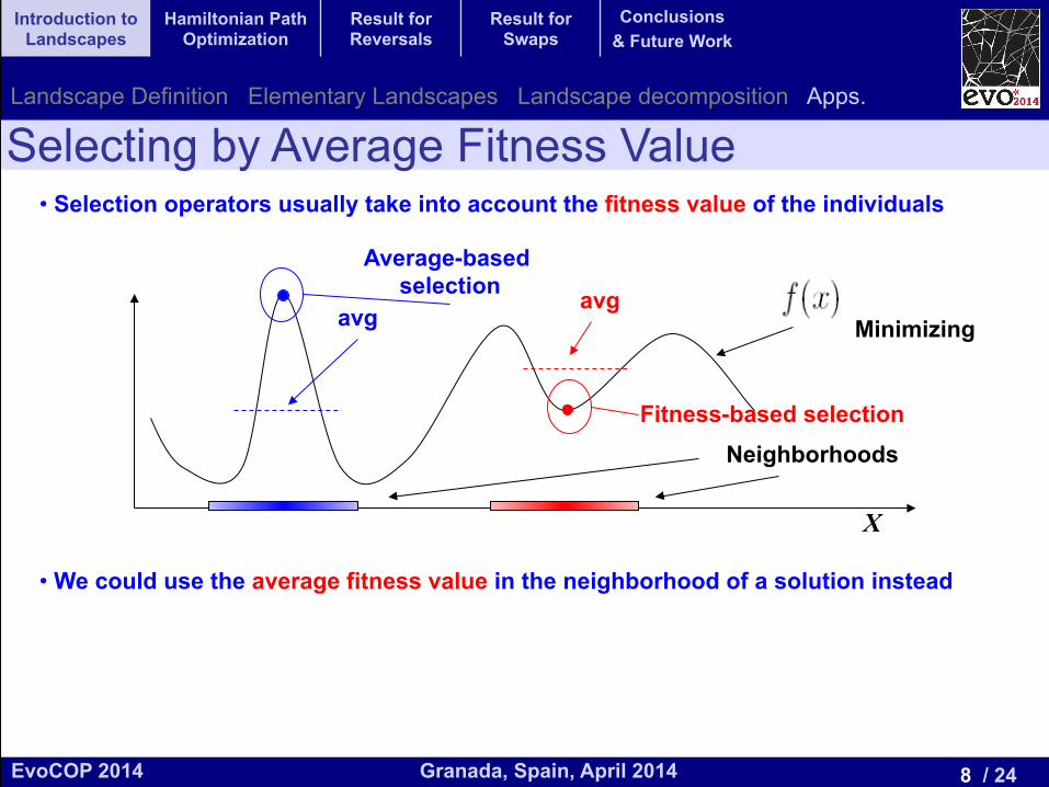
•  Selection operators usually take into account the fitness value of the individuals

•  We could use the average fitness value in the neighborhood of a solution instead

Selecting by Average Fitness Value

X

Neighborhoods

avg avg

Minimizing

Fitness-based selection

Average-based selection




Result for Swaps





CONFERENCE'HANDBOOK

•  In elementary landscapes the traditional and the new operator are the same!

Recall that...

•  However, they are not the same in non-elementary landscapes. If we have n elementary components, then:

•  This selection strategy could be useful for plateaus Elementary components

X

Minimizing

avg avg

Fitness-based selection Average-based

selection

?

Selecting by Average Fitness Value




Result for Swaps





CONFERENCE'HANDBOOK

•  Let {x0, x1, ...} a simple random walk on the configuration space where xi+1∈N(xi)

•  The random walk induces a time series {f(x0), f(x1), ...} on a landscape.

•  The autocorrelation function is defined as:

•  The autocorrelation length and coefficient:

•  Autocorrelation length “conjecture”:

Autocorrelation

s0

s4 s7

s6

s2

s1

s8 s9

s5

s3 2

0

3

5

1

2

4 0

7 6

The number of local optima in a search space is roughly Solutions reached from x0

after l moves




Result for Swaps





CONFERENCE'HANDBOOK

Hamiltonian Path Optimization (HPO) Definition Neighborhoods

•  In TSP we search for a Hamiltonian circuit with minimal cost

•  In HPO we search for a Hamiltonian path with minimal cost

•  Applications:

•  DNA fragment assembly (usually not solved as such)

•  DNA linkage marker sequencing (solved as HPO)

6

1

2

3

5

4

(1,2,3,4,5)

6

1

2

3

5

4

(1,2,3,4,5)

↵

d

�

d

f̄ =�

↵+ �

X

c2C

w(c)

f(⇡) =n�1X

i=1

w⇡(i),⇡(i+1) + w⇡(n),⇡(1)

1




Result for Swaps




CONFERENCE'HANDBOOK

Neighborhoods •  We investigate two different neighborhoods: (reduced) reversals and swaps

2 4 3 5 1 6

2 1 5 3 4 6

(a) Reversal

2 4 3 5 1 6

2 1 3 5 4 6

(b) Swap

Fig. 1. Examples of reversal and swap for a permutation of size 6.

4.1 Component Model

Whitley and Sutton developed a “component” based model that makes it easy toidentify elementary landscapes [17]. Let C be a set of “components” of a problem.Each component c 2 C has a weight (or cost) denoted by w(c). A solution x ✓ C

is a subset of components and the evaluation function f(x) maps each solution x

to the sum of the weights of the components in x: f(x) =P

c2x

w(c). Finally, letC �x denote the subset of components that do not contribute to the evaluationof solution x. Note that the sum of the weights of the components in C � x iscomputed by

Pc2C

w(c)�f(x). In the context of the component model, Grover’swave equation can be expressed as:

Avg(f(y))y2N(x)

= f(x)� p1f(x) + p2

X

c2C

w(c)� f(x)

!,

where p1 = ↵/d is the (sampling) rate at which components that contribute tof(x) are removed from solution x to create a neighboring solution y 2 N(x),and p2 = �/d is the rate at which components in the set C � x are sampled tocreate a neighboring solution y 2 N(x). By simple algebra,

Avg(f(y))y2N(x)

= f(x)� p1f(x) + p2

X

w2C

w(c)� f(x)

!= f(x) +

�

d

(f̄ � f(x)),

where � = ↵+ �, and f̄ = �/(↵+ �)P

c2C

w(c) [16].

4.2 Proof of Elementariness

Let us start presenting two lemmas.

Lemma 1. Given the n! possible Hamiltonian Paths over n vertices, all edgesappear the same number of times in the n! solutions and this number is 2(n�1)!.

Proof. Each edge (u, v) of the graph can be placed in positions 1, 2, . . . , n � 1of the permutation. This means a total of n � 1 positions where (u, v) can beplaced. For each position it can appear as u followed by v or v followed by u.

Reversal

The solutions for the HPO problem can be modeled as permutations, whichindicate in which order all the vertices are visited. Let us number all the verticesof the graph and let w be the weight matrix, which we will consider symmetric,where w

p,q

is the weight of the edge (p, q). The fitness function for HPO is:

f(⇡) =n�1X

i=1

w

⇡(i),⇡(i+1), (2)

where ⇡ is a permutation and ⇡(i) is the i-th element in that permutation. HPOis a subtype of a more general problem: the Quadratic Assignment Problem(QAP) [2]. Given two matrices r and w the fitness function of QAP is:

f

QAP

(⇡) =nX

i,j=1

r

i,j

w

⇡(i),⇡(j). (3)

We can observe that (3) generalizes (2) if w is the weight matrix for HPOand we define r

i,j

= �

j

i+1, where � is the Kronecker delta. HPO has applica-tions in Bioinformatics, in particular in DNA fragment assembling [10] and theconstruction of radiation hybrid maps [1].

4 Landscape for Reversals

Given a permutation ⇡ and two positions i and j with 1 i < j n, we canform a new permutation ⇡

0 by reversing the elements between i and j (inclusive).Formally, the new permutation is defined as:

⇡

0(k) =

⇢⇡(k) if k < i or k > j,⇡(j + i� k) if i k j.

(4)

Figure 1(a) illustrates the concept of reversal. The reversal neighborhoodN

R

(⇡) of a permutation ⇡ contains all the permutations that can be formed byapplying reversals to ⇡. Each reversal can be identified by a pair [i, j], which arethe starting and ending positions of the reversal. We use square brackets in thereversals to distinguish them from swaps. Then, we have |N

R

(⇡)| = n(n� 1)/2.In the context of HPO, where we consider a symmetric cost matrix, the

solution we obtain after applying the reversal [i, j] = [1, n] to ⇡ has the sameobjective value as ⇡, since it is simply a reversal of the complete permutation.For this reason, we will remove this reversal from the neighborhood. We willcall the new neighborhood the reduced reversal neighborhood, denoted with N

RR

to distinguish it from the original reversal neighborhood. We have |NRR

(⇡)| =n(n�1)/2�1. In the remaining of this section we will refer always to the reducedreversal neighborhood unless otherwise stated. The landscape analyzed in thissection is composed of the set of permutations of n elements, the reduced reversalneighborhood and the objective function (2). We will use the component modelexplained in the next section to prove that this landscape is elementary.

Swap

and all feasible locations j < i. When all possible values of j are considered,this causes all of the vertices in the permutation left of vertex v

i

to come into aposition adjacent to v

i

except for vi�1 which is already adjacent. Next consider a

cut at location i+1 (i is still fixed) and all feasible locations m > i+1. When allof the possible of value of m are considered all of the vertices in the permutationto the right of vertex v

i

are moved into a position adjacent to v

i

except v

i+1.Thus, in these cases v

i

does not move, but every edge not in the solution x

that is incident on vertex i is sampled once. Since this is true for all vertices, itfollows that every edge not in the current solution is sampled twice (� = 2): oncefor each of the vertices in which it is incident. Therefore, summing over all theneighbors: d ·Avg(f(y))

y2N(x) = d · f(x)� (n� 2)f(x)+ 2�P

c2C

w(c)� f(x)�.

Computing the average over the neighborhood and taking into account theresult of Lemma 2:

Avg(f(y))y2N(x)

= f(x)� n� 2

n(n� 1)/2� 1f(x) +

2

n(n� 1)/2� 1

X

c2C

w(c)� f(x)

!

= f(x) +n

n(n� 1)/2� 1(f̄ � f(x)).

ut

5 Landscape Structure for Swaps

Given a permutation ⇡, we can build a new permutation ⇡

0 by swapping twopositions i and j in the permutation. The new permutation is defined as:

⇡

0(k) =

8<

:

⇡(k) if k 6= i and k 6= j,⇡(i) if k = j,⇡(j) if k = i.

(5)

Figure 1(b) illustrates the concept of swap. The swap neighborhood N

S

(⇡) ofa permutation ⇡ contains all the permutations that can be formed by applyingswaps to ⇡. Each swap can be identified by the pair (i, j) of positions to swap. Thecardinality of the swap neighborhood is |N

S

(⇡)| = n(n� 1)/2. Unless otherwisestated, we will refer always to the swap neighborhood in this section.

We will analyze the landscape composed of the set of permutations of n

elements, the swap neighborhood and the objective function (2). The approachused for this analysis will be di↵erent than the one in the previous section.Instead of using the component model we will base our results in the analysis ofthe QAP landscape done in [6]. The reasons for not using the component modelwill be discussed at the end of the section.

5.1 Previous Results for QAP

According to Chicano et al. [6], the ELD of the QAP for the swap neighborhoodis composed of three components. The objective function analyzed in [6] is moregeneral than (3), it corresponds to the Lawler version of QAP [9]:

2 4 3 5 1 6

2 1 5 3 4 6

(a) Reversal

2 4 3 5 1 6

2 1 3 5 4 6

(b) Swap


4.1 Component Model




c2x


Pc2C


Avg(f(y))y2N(x)

= f(x)� p1f(x) + p2

X

c2C

w(c)� f(x)

!,


Avg(f(y))y2N(x)

= f(x)� p1f(x) + p2

X

w2C

w(c)� f(x)

!= f(x) +

�

d

(f̄ � f(x)),

where � = ↵+ �, and f̄ = �/(↵+ �)P

c2C

w(c) [16].





•  We call it “reduced” reversals because we omit the reversal of the whole permutation




Result for Swaps


Definition Neighborhoods



CONFERENCE'HANDBOOK

Component Model (Whitley, Sutton, Howe)

Component Model Elementariness

•  Let C be a set of components, each component having a weight w(c)

•  A solution x is a subset of C:

•  The fitness value of x is the sum of the weights of the components in x:

•  Let us consider a neighbor y of x, we can classify the components in x and y as:

•  Components that are in both solutions

•  Components that are in x and not in y (removed from x when we move to y)

•  Components that are in y and not in x (included from C-x when we move to y)




Result for Swaps


2 4 3 5 1 6

2 1 5 3 4 6

(a) Reversal

2 4 3 5 1 6

2 1 3 5 4 6

(b) Swap


4.1 Component Model




c2x


Pc2C


Avg(f(y))y2N(x)

= f(x)� p1f(x) + p2

X

c2C

w(c)� f(x)

!,


Avg(f(y))y2N(x)

= f(x)� p1f(x) + p2

X

w2C

w(c)� f(x)

!= f(x) +

�

d

(f̄ � f(x)),

where � = ↵+ �, and f̄ = �/(↵+ �)P

c2C

w(c) [16].





2 4 3 5 1 6

2 1 5 3 4 6

(a) Reversal

2 4 3 5 1 6

2 1 3 5 4 6

(b) Swap


4.1 Component Model




c2x


Pc2C


Avg(f(y))y2N(x)

= f(x)� p1f(x) + p2

X

c2C

w(c)� f(x)

!,


Avg(f(y))y2N(x)

= f(x)� p1f(x) + p2

X

w2C

w(c)� f(x)

!= f(x) +

�

d

(f̄ � f(x)),

where � = ↵+ �, and f̄ = �/(↵+ �)P

c2C

w(c) [16].





2 4 3 5 1 6

2 1 5 3 4 6

(a) Reversal

2 4 3 5 1 6

2 1 3 5 4 6

(b) Swap


4.1 Component Model




c2x


Pc2C


Avg(f(y))y2N(x)

= f(x)� p1f(x) + p2

X

c2C

w(c)� f(x)

!,


Avg(f(y))y2N(x)

= f(x)� p1f(x) + p2

X

w2C

w(c)� f(x)

!= f(x) +

�

d

(f̄ � f(x)),

where � = ↵+ �, and f̄ = �/(↵+ �)P

c2C

w(c) [16].





2 4 3 5 1 6

2 1 5 3 4 6

(a) Reversal

2 4 3 5 1 6

2 1 3 5 4 6

(b) Swap


4.1 Component Model




c2x


Pc2C


Avg(f(y))y2N(x)

= f(x)� p1f(x) + p2

X

c2C

w(c)� f(x)

!,


Avg(f(y))y2N(x)

= f(x)� p1f(x) + p2

X

w2C

w(c)� f(x)

!= f(x) +

�

d

(f̄ � f(x)),

where � = ↵+ �, and f̄ = �/(↵+ �)P

c2C

w(c) [16].





6

1

2

3

5

4

(1,2,3,4,5)

1 2

3

4 5

6 6

1

2

3

5

4

(1,2,3,4,5)

1 2

3

4 5

6 x

y



CONFERENCE'HANDBOOK

Component Theorem (Whitley, Sutton, Howe) •  Let us assume that generating a symmetric neighborhood it happens that:

•  All the components IN x are removed the same number of times, α

•  All the components in C-x (OUT of x) are included the same number of times, β

•  Then, the landscape is elementary

•  And the wave equation is:

•  where

6

1

2

3

5

4

(1,2,3,4,5)

1 2

3

4 5

6

2 4 3 5 1 6

2 1 5 3 4 6

(a) Reversal

2 4 3 5 1 6

2 1 3 5 4 6

(b) Swap


4.1 Component Model




c2x


Pc2C


Avg(f(y))y2N(x)

= f(x)� p1f(x) + p2

X

c2C

w(c)� f(x)

!,


Avg(f(y))y2N(x)

= f(x)� p1f(x) + p2

X

w2C

w(c)� f(x)

!= f(x) +

�

d

(f̄ � f(x)),

where � = ↵+ �, and f̄ = �/(↵+ �)P

c2C

w(c) [16].





2 4 3 5 1 6

2 1 5 3 4 6

(a) Reversal

2 4 3 5 1 6

2 1 3 5 4 6

(b) Swap


4.1 Component Model




c2x


Pc2C


Avg(f(y))y2N(x)

= f(x)� p1f(x) + p2

X

c2C

w(c)� f(x)

!,


Avg(f(y))y2N(x)

= f(x)� p1f(x) + p2

X

w2C

w(c)� f(x)

!= f(x) +

�

d

(f̄ � f(x)),

where � = ↵+ �, and f̄ = �/(↵+ �)P

c2C

w(c) [16].





2 4 3 5 1 6

2 1 5 3 4 6

(a) Reversal

2 4 3 5 1 6

2 1 3 5 4 6

(b) Swap


4.1 Component Model




c2x


Pc2C


Avg(f(y))y2N(x)

= f(x)� p1f(x) + p2

X

c2C

w(c)� f(x)

!,


Avg(f(y))y2N(x)

= f(x)� p1f(x) + p2

X

w2C

w(c)� f(x)

!= f(x) +

�

d

(f̄ � f(x)),

where � = ↵+ �, and f̄ = �/(↵+ �)P

c2C

w(c) [16].





↵

d

�

d

1

↵

d

�

d

1

↵

d

�

d

f̄ =�

↵+ �

X

c2C

w(c)

1

Does not change with the neighborhood

IN OUT




Result for Swaps





CONFERENCE'HANDBOOK

Elementariness of HPO with reversals: IN •  How many times is a component IN the solution removed in the neighborhood?

α = n-2




Result for Swaps





CONFERENCE'HANDBOOK

Elementariness of HPO with reversals: IN •  How many times is a component OUT of the solution included in the neighborhood?

•  HPO with reversals is elementary and the wave equation is:

β = 2

and all feasible locations j < i. When all possible values of j are considered,this causes all of the vertices in the permutation left of vertex v

i

to come into aposition adjacent to v

i

except for vi�1 which is already adjacent. Next consider a

cut at location i+1 (i is still fixed) and all feasible locations m > i+1. When allof the possible of value of m are considered all of the vertices in the permutationto the right of vertex v

i

are moved into a position adjacent to v

i

except v

i+1.Thus, in these cases v

i

does not move, but every edge not in the solution x

that is incident on vertex i is sampled once. Since this is true for all vertices, itfollows that every edge not in the current solution is sampled twice (� = 2): oncefor each of the vertices in which it is incident. Therefore, summing over all theneighbors: d ·Avg(f(y))

y2N(x) = d · f(x)� (n� 2)f(x)+ 2�P

c2C

w(c)� f(x)�.

Computing the average over the neighborhood and taking into account theresult of Lemma 2:

Avg(f(y))y2N(x)

= f(x)� n� 2

n(n� 1)/2� 1f(x) +

2

n(n� 1)/2� 1

X

c2C

w(c)� f(x)

!

= f(x) +n

n(n� 1)/2� 1(f̄ � f(x)).

ut

5 Landscape Structure for Swaps

Given a permutation ⇡, we can build a new permutation ⇡

0 by swapping twopositions i and j in the permutation. The new permutation is defined as:

⇡

0(k) =

8<

:

⇡(k) if k 6= i and k 6= j,⇡(i) if k = j,⇡(j) if k = i.

(5)

Figure 1(b) illustrates the concept of swap. The swap neighborhood N

S

(⇡) ofa permutation ⇡ contains all the permutations that can be formed by applyingswaps to ⇡. Each swap can be identified by the pair (i, j) of positions to swap. Thecardinality of the swap neighborhood is |N

S

(⇡)| = n(n� 1)/2. Unless otherwisestated, we will refer always to the swap neighborhood in this section.

We will analyze the landscape composed of the set of permutations of n

elements, the swap neighborhood and the objective function (2). The approachused for this analysis will be di↵erent than the one in the previous section.Instead of using the component model we will base our results in the analysis ofthe QAP landscape done in [6]. The reasons for not using the component modelwill be discussed at the end of the section.

5.1 Previous Results for QAP

According to Chicano et al. [6], the ELD of the QAP for the swap neighborhoodis composed of three components. The objective function analyzed in [6] is moregeneral than (3), it corresponds to the Lawler version of QAP [9]:




Result for Swaps





CONFERENCE'HANDBOOK

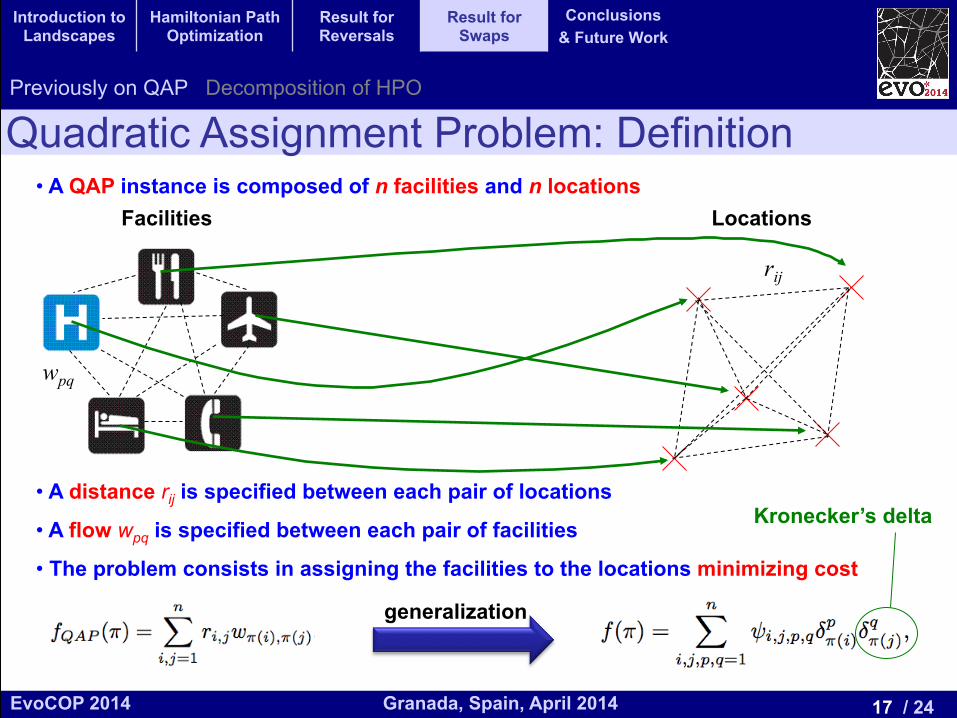
Quadratic Assignment Problem: Definition Previously on QAP Decomposition of HPO

rij

•  A QAP instance is composed of n facilities and n locations

•  A distance rij is specified between each pair of locations

•  A flow wpq is specified between each pair of facilities

•  The problem consists in assigning the facilities to the locations minimizing cost

wpq

Facilities Locations

generalization

Kronecker’s delta




Result for Swaps




CONFERENCE'HANDBOOK

QAP Decomposition (Chicano, Whitley, Alba) •  Auxiliary ϕ functions

•  Three elementary components for the swap neighborhood

p … q

i j π

q … p

Eigenvalues




Result for Swaps


Previously on QAP Decomposition of HPO



CONFERENCE'HANDBOOK

•  The three components of QAP

Kronecker’s delta

QAP Decomposition (Chicano, Whitley, Alba)




Result for Swaps





CONFERENCE'HANDBOOK

•  If any of the matrices w or r is symmetric, then f2n is a constant

•  If any of the matrices w or r is antisymmetric, then f2(n-1) is a constant

Properties of the decomposition




Result for Swaps





CONFERENCE'HANDBOOK

•  TSP is a particular case of QAP with two elementary components: f2n and f2(n-1)

•  HPO is another subproblem of QAP

Subproblems of QAP: TSP and HPO

↵

d

�

d

f̄ =�

↵+ �

X

c2C

w(c)

f(⇡) =n�1X

i=1

w⇡(i),⇡(i+1) + w⇡(n),⇡(1)

1




Result for Swaps





CONFERENCE'HANDBOOK

•  If distance matrix in HPO is symmetric then f2n is a constant and the landscape has two elementary components:

Subproblems of QAP: TSP and HPO




Result for Swaps





CONFERENCE'HANDBOOK

•  HPO with the reduced reversals neighborhood is an elementary landscape

•  HPO with the swap neighborhood is the sum of two elementary landscapes

•  The analysis of the problem can be used to compute statistics that could help in the search

•  Spectral theory of quasi-Abelian Cayley graph cannot be easily applied to the reversals

Conclusions

Future Work

•  Analysis of partial neighborhoods

•  Search for additional applications of the elementary landscape decomposition

•  How do the elementary components of HPO relate to the equivalent TSP problem?





Result for Swaps




CONFERENCE'HANDBOOK

Thanks for your attention !!!

Elementary Landscape Decomposition of the Hamiltonian Path Optimization Problem

Elementary Landscape Decomposition of the Hamiltonian Path Optimization Problem

Science

Transcript of Elementary Landscape Decomposition of the Hamiltonian Path Optimization Problem