Elementary Introduction to Quantum Fields in

Curved Spacetime

Lecture notes by Sergei Winitzki

Heidelberg, April 18-21, 2006

Contents

Preface . . . . . . . . . . . . . . . . . . . . . . . . . . . . . . . . . . . . . . . 2Suggested literature . . . . . . . . . . . . . . . . . . . . . . . . . . . . . . . . 3

1 Quantization of harmonic oscillator 31.1 Canonical quantization . . . . . . . . . . . . . . . . . . . . . . . . . . . 31.2 Creation and annihilation operators . . . . . . . . . . . . . . . . . . . 41.3 Particle number eigenstates . . . . . . . . . . . . . . . . . . . . . . . . 5

2 Quantization of scalar field 62.1 Classical field . . . . . . . . . . . . . . . . . . . . . . . . . . . . . . . . 62.2 Quantization of scalar field . . . . . . . . . . . . . . . . . . . . . . . . 72.3 Mode expansions . . . . . . . . . . . . . . . . . . . . . . . . . . . . . . 9

3 Casimir effect 93.1 Zero-point energy . . . . . . . . . . . . . . . . . . . . . . . . . . . . . . 93.2 Casimir effect . . . . . . . . . . . . . . . . . . . . . . . . . . . . . . . . 103.3 Zero-point energy between plates . . . . . . . . . . . . . . . . . . . . . 103.4 Regularization and renormalization . . . . . . . . . . . . . . . . . . . 13

4 Oscillator with varying frequency 144.1 Quantization . . . . . . . . . . . . . . . . . . . . . . . . . . . . . . . . . 144.2 Choice of mode function . . . . . . . . . . . . . . . . . . . . . . . . . . 164.3 “In” and “out” states . . . . . . . . . . . . . . . . . . . . . . . . . . . . 174.4 Relationship between “in” and “out” states . . . . . . . . . . . . . . . 194.5 Quantum-mechanical analogy . . . . . . . . . . . . . . . . . . . . . . 20

5 Scalar field in expanding universe 215.1 Curved spacetime . . . . . . . . . . . . . . . . . . . . . . . . . . . . . 215.2 Scalar field in cosmological background . . . . . . . . . . . . . . . . . 225.3 Mode expansion . . . . . . . . . . . . . . . . . . . . . . . . . . . . . . . 235.4 Quantization of scalar field . . . . . . . . . . . . . . . . . . . . . . . . 245.5 Vacuum state and particle states . . . . . . . . . . . . . . . . . . . . . 255.6 Bogolyubov transformations . . . . . . . . . . . . . . . . . . . . . . . 255.7 Mean particle number . . . . . . . . . . . . . . . . . . . . . . . . . . . 265.8 Instantaneous lowest-energy vacuum . . . . . . . . . . . . . . . . . . 275.9 Computation of Bogolyubov coefficients . . . . . . . . . . . . . . . . . 27

1

6 Amplitude of quantum fluctuations 296.1 Fluctuations of averaged fields . . . . . . . . . . . . . . . . . . . . . . 296.2 Fluctuations in Minkowski spacetime . . . . . . . . . . . . . . . . . . 306.3 de Sitter spacetime . . . . . . . . . . . . . . . . . . . . . . . . . . . . . 306.4 Quantum fields in de Sitter spacetime . . . . . . . . . . . . . . . . . . 316.5 Bunch-Davies vacuum state . . . . . . . . . . . . . . . . . . . . . . . . 326.6 Spectrum of fluctuations in the BD vacuum . . . . . . . . . . . . . . . 33

7 Unruh effect 337.1 Kinematics of uniformly accelerated motion . . . . . . . . . . . . . . 347.2 Coordinates in the proper frame . . . . . . . . . . . . . . . . . . . . . 357.3 Rindler spacetime . . . . . . . . . . . . . . . . . . . . . . . . . . . . . . 387.4 Quantum field in Rindler spacetime . . . . . . . . . . . . . . . . . . . 387.5 Lightcone mode expansions . . . . . . . . . . . . . . . . . . . . . . . . 417.6 Bogolyubov transformations . . . . . . . . . . . . . . . . . . . . . . . . 427.7 Density of particles . . . . . . . . . . . . . . . . . . . . . . . . . . . . . 447.8 Unruh temperature . . . . . . . . . . . . . . . . . . . . . . . . . . . . . 47

8 Hawking radiation 478.1 Scalar field in Schwarzschild spacetime . . . . . . . . . . . . . . . . . 488.2 Kruskal coordinates . . . . . . . . . . . . . . . . . . . . . . . . . . . . . 498.3 Field quantization . . . . . . . . . . . . . . . . . . . . . . . . . . . . . . 508.4 Choice of vacuum . . . . . . . . . . . . . . . . . . . . . . . . . . . . . . 518.5 Hawking temperature . . . . . . . . . . . . . . . . . . . . . . . . . . . 528.6 Black hole thermodynamics . . . . . . . . . . . . . . . . . . . . . . . . 53

A Hilbert spaces and Dirac notation 55A.1 Infinite-dimensional vector spaces . . . . . . . . . . . . . . . . . . . . 55A.2 Dirac notation . . . . . . . . . . . . . . . . . . . . . . . . . . . . . . . . 55A.3 Hermiticity . . . . . . . . . . . . . . . . . . . . . . . . . . . . . . . . . 56A.4 Hilbert spaces . . . . . . . . . . . . . . . . . . . . . . . . . . . . . . . . 57

B Mode expansions cheat sheet 58

Preface

This course is a brief introduction to Quantum Field Theory in Curved Spacetime(QFTCS)—a beautiful and fascinating area of fundamental physics. The applica-tion of QFTCS is required in situations when both gravitation and quantum me-chanics play a significant role, for instance, in early-universe cosmology and blackhole physics. The goal of this course is to introduce some of the most accessibleaspects of quantum theory in nontrivial backgrounds and to explain its most unex-pected and spectacular manifestations—the Casimir effect (uncharged metal platesattract), the Unruh effect (an accelerated observer will detect particles in vacuum),and Hawking’s theoretical discovery of black hole radiation (black holes are notcompletely black).

This short course was taught in the framework of Heidelberger Graduiertenkurseat the Heidelberg University (Germany) in the Spring of 2006. The audience in-cluded advanced undergraduates and beginning graduate students. Only a basicfamiliarity with quantum mechanics, electrodynamics, and general relativity is re-quired. The emphasis is on concepts and intuitive explanations rather than oncomputational techniques. The relevant calculations are deliberately simplifiedas much as possible, while retaining all the relevant physics. Some remarks andderivations are typeset in smaller print and can be skipped at first reading.

2

These lecture notes are freely based on an early draft of the book [MW07] withsome changes appropriate for the purposes of the Heidelberg course. The presenttext may be freely distributed according to the GNU Free Documentation License.1

Sergei Winitzki, April 2006

Suggested literature

The following more advanced books may be studied as a continuation of this in-troductory course:

[BD82] N. D. BIRRELL and P. C. W. DAVIES, Quantum fields in curved space(Cambridge University Press, 1982).

[F89] S. A. FULLING, Aspects of quantum field theory in curved space-time (Cam-bridge University Press, 1989).

[GMM94] A. A. GRIB, S. G. MAMAEV, and V. M. MOSTEPANENKO, Vacuumquantum effects in strong fields (Friedmann Laboratory Publishing, St. Petersburg,1994).

The following book contains a significantly more detailed presentation of thematerial of this course, and much more:

[MW07] V. F. MUKHANOV and S. WINITZKI, Quantum Effects in Gravity (to bepublished by Cambridge University Press, 2007).2

1 Quantization of harmonic oscillator

This section serves as a very quick reminder of quantum mechanics of harmonicoscillators. It is assumed that the reader is already familiar with such notions asSchrödinger equation and Heisenberg picture.

1.1 Canonical quantization

A classical harmonic oscillator is described by a coordinate q(t) satisfying

q + ω2q = 0, (1)

where ω is a real constant. The general solution of this equation can be written as

q(t) = aeiωt + a∗e−iωt,

where a is a (complex-valued) constant. We may identify the “ground state” of theoscillator as the state without motion, i.e. q(t) ≡ 0. This is obviously the lowest-energy state of the oscillator.

The quantum theory of the oscillator is obtained by the standard procedureknown as canonical quantization. Canonical quantization does not apply directlyto an equation of motion. Rather, we first need to describe the system using theHamiltonian formalism, which means that we must start with the Lagrangian ac-tion principle. The classical equation of motion (1) is reformulated as a conditionto extremize the action,

∫

L(q, q)dt =

∫[

1

2q2 − 1

2ω2q2

]

dt,

1See www.gnu.org/copyleft/fdl.html2An early, incomplete draft is available at www.theorie.physik.uni-muenchen.de/~serge/T6/

3

where the function L(q, q) is the Lagrangian. (For simplicity, we assumed a unitmass of the oscillator.) Then we define the canonical momentum

p ≡ ∂L(q, q)

∂q= q,

and perform a Legendre transformation to find the Hamiltonian

H(p, q) ≡ [pq − L]q→p =1

2p2 +

1

2ω2q2.

The Hamiltonian equations of motion are

q = p, p = −ω2q.

Finally, we replace the classical coordinate q(t) and the momentum p(t) by Hermi-tian operators q(t) and p(t) satisfying the same equations of motion,

˙q = p, ˙p = −ω2q,

and additionally postulate the Heisenberg commutation relation

[q(t), p(t)] = i~. (2)

The Hamiltonian H(p, q) is also promoted to an operator,

H ≡ H(p, q) =1

2p2 +

1

2ω2q2.

All the quantum operators pertaining to the oscillator act in a certain vector spaceof quantum states or wavefunctions. (This space must be a Hilbert space; see Ap-pendix A for details.) Vectors from this space are usually denoted using Dirac’s“bra-ket” symbols: vectors are denoted by |a〉, |b〉, and the corresponding covec-tors by 〈a|, 〈b|, etc. Presently, we use the Heisenberg picture, in which the opera-tors depend on time but the quantum states are time-independent. This picture ismore convenient for developing quantum field theory than the Schrödinger pic-ture where operators are time-independent but wavefunctions change with time.Therefore, we shall continue to treat the harmonic oscillator in the Heisenberg pic-ture. We shall not need to use the coordinate or momentum representation ofwavefunctions.

1.2 Creation and annihilation operators

The “classical ground state” q(t) ≡ 0 is impossible in quantum theory because inthat case the commutation relation (2) could not be satisfied by any p(t). Hence, aquantum oscillator cannot be completely at rest, and its lowest-energy state (calledthe ground state or the vacuum state) has a more complicated structure. The stan-dard way of describing quantum oscillators is through the introduction of the cre-ation and annihilation operators.

From now on, we use the units where ~ = 1. The Heisenberg commutationrelation becomes

[q(t), p(t)] = i. (3)

We now define the annihilation operator a−(t) and its Hermitian conjugate, cre-ation operator a+(t), by

a±(t) =

√

ω

2

[

q(t) ∓ i

ωp(t)

]

.

4

These operators are not Hermitian since (a−)† = a+. The equation of motion forthe operator a−(t) is straightforward to derive,

d

dta−(t) = −iωa−(t). (4)

(The Hermitian conjugate operator a+(t) satisfies the complex conjugate equation.)The solution of Eq. (4) with the initial condition a−(t)|t=0 = a−0 can be readilyfound,

a−(t) = a−0 e−iωt. (5)

It is helpful to introduce time-independent operators a±0 ≡ a± and to write thetime-dependent phase factor eiωt explicitly. For instance, we find that the canonicalvariables p(t), q(t) are related to a± by

p(t) =√ωa−e−iωt − a+eiωt

i√

2, q(t) =

a−e−iωt + a+eiωt

√2ω

. (6)

From now on, we shall only use the time-independent operators a±. Using Eqs. (3)and (6), it is easy to show that

[a−, a+] = 1.

Using the relations (6), the operator H can be expressed through the creation andannihilation operators a± as

H =

(

a+a− +1

2

)

ω. (7)

1.3 Particle number eigenstates

Quantum states of the oscillator are described by vectors in an appropriate (infinite-dimensional) Hilbert space. A complete basis in this space is made of vectors |0〉,|1〉, ..., which are called the occupation number states or particle number states.The construction of these states is well known, and we briefly review it here forcompleteness.

It is seen from Eq. (7) that the eigenvalues of H are bounded from below by12ω. It is then assumed that the ground state |0〉 exists and is unique. Using thisassumption and the commutation relations, one can show that the state |0〉 satisfies

a− |0〉 = 0.

(This derivation is standard and we omit it here.) Then we have H |0〉 = 12ω |0〉,

which means that the ground state |0〉 indeed has the lowest possible energy 12ω.

The excited states |n〉, where n = 1, 2, ..., are defined by

|n〉 =1√n!

(a+)n |0〉 . (8)

The factors√n! are needed for normalization, namely 〈m|n〉 = δmn. It is easy to

see that every state |n〉 is an eigenstate of the Hamiltonian,

H |n〉 =

(

n+1

2

)

ω |n〉 .

In other words, the energy of the oscillator is quantized (not continuous) and is mea-sured in discrete “quanta” equal to ω. Therefore, we might interpret the state |n〉as describing the presence of n “quanta” of energy or n “particles,” each “particle”

5

having the energy ω. (In normal units, the energy of each quantum is ~ω, which

is the famous Planck formula for the energy quantum.) The operator N ≡ a+a−

is called the particle number operator. Since N |n〉 = n |n〉, the states |n〉 are alsocalled particle number eigenstates. This terminology is motivated by the applica-tions in quantum field theory (as we shall see below).

To get a feeling of what the ground state |0〉 looks like, one can compute the ex-pectation values of the coordinate and the momentum in the state |0〉. For instance,using Eq. (6) we find

〈0| q(t) |0〉 = 0, 〈0| p(t) |0〉 = 0,

〈0| q2(t) |0〉 =1

2ω, 〈0| p2(t) |0〉 =

ω

2.

It follows that the ground state |0〉 of the oscillator exhibits fluctuations of both thecoordinate and the momentum around a zero mean value. The typical value of the

fluctuation in the coordinate is δq ∼ (2ω)−1/2

.

2 Quantization of scalar field

The quantum theory of fields is built on two essential foundations: the classicaltheory of fields and the quantum mechanics of harmonic oscillators.

2.1 Classical field

A classical field is described by a function of spacetime, φ (x, t), characterizing thelocal strength or intensity of the field. Here x is a three-dimensional coordinate inspace and t is the time (in some reference frame). The function φ (x, t) may havereal values, complex values, or values in some finite-dimensional vector space. Forexample, the electromagnetic field is described by the 4-potential Aµ(x, t), whichis a function whose values are 4-vectors.

The simplest example of a field is a real scalar field φ (x, t); its values are realnumbers. A free, massive scalar field satisfies the Klein-Gordon equation3

∂2φ

∂t2−

3∑

j=1

∂2φ

∂x2j

+m2φ ≡ φ− ∆φ+m2φ ≡ ∂µ∂µφ+m2φ = 0. (9)

The parameter m is the mass of the field. The solution φ (x, t) ≡ 0 is the classicalvacuum state (“no field”).

To simplify the equations of motion, it is convenient to use the spatial Fourierdecomposition,

φ (x, t) =

∫

d3k

(2π)3/2eik·xφk(t), (10)

where we integrate over all three-dimensional vectors k. After the Fourier decom-position, the partial differential equation (9) is replaced by infinitely many ordi-nary differential equations, with one equation for each k:

φk +(

k2 +m2)

φk = φk + ω2kφk = 0, ωk ≡

√

|k|2 +m2.

In other words, each function φk(t) satisfies the harmonic oscillator equation withthe frequency ωk. The complex-valued functions φk(t) are called the modes of the

3To simplify the formulas, we shall (almost always) use the units in which ~ = c = 1.

6

field φ (abbreviated from “Fourier modes”). Note that the modes φk(t) of a realfield φ(x, t) satisfy the relation (φk)∗ = φ−k.

The equation of motion (9) can be found by extremizing the action

S [φ] =1

2

∫

d4x[

ηµν (∂µφ) (∂νφ) −m2φ2]

≡ 1

2

∫

d3x dt[

φ2 − (∇φ)2 −m2φ2]

, (11)

where ηµν = diag(1,−1,−1,−1) is the Minkowski metric (in this chapter we con-sider only the flat spacetime) and the Greek indices label four-dimensional coor-dinates: x0 ≡ t and (x1, x2, x3) ≡ x. Using Eq. (10), one can also express theaction (11) directly through the (complex-valued) modes φk,

S =1

2

∫

dt d3k

[

φkφ∗k − ω2

kφkφ∗k

]

. (12)

2.2 Quantization of scalar field

The action (12) is analogous to that of a collection of infinitely many harmonicoscillators. Therefore, we may quantize each mode φk(t) as a separate (complex-valued) harmonic oscillator.

Let us begin with the Hamiltonian description of the field φ(x, t). The ac-tion (11) must be thought of as an integral of the Lagrangian over time (but notover space), S[φ] =

∫

L[φ] dt, so the Lagrangian L[φ] is

L[φ] =

∫

Ld3x; L ≡ 1

2ηµν (∂µφ) (∂νφ) − 1

2m2φ2,

where L is the Lagrangian density. To define the canonical momenta and theHamiltonian, one must use the LagrangianL[φ] rather than the Lagrangian densityL. Hence, the momenta π (x, t) are computed as the functional derivatives

π (x, t) ≡ δL [φ]

δφ (x, t)= φ (x, t) ,

and then the classical Hamiltonian is

H =

∫

π (x, t) φ (x, t) d3x − L =1

2

∫

d3x[

π2 + (∇φ)2 +m2φ2]

. (13)

To quantize the field, we introduce the operators φ (x, t) and π (x, t) with thestandard commutation relations

[φ (x, t) , π (y, t)] = iδ (x − y) ; [φ (x, t) , φ (y, t)] = [π (x, t) , π (y, t)] = 0. (14)

The modes φk(t) also become operators φk(t). The commutation relation for themodes can be derived from Eq. (14) by performing Fourier transforms in x and y.After some algebra, we find

[

φk(t), πk′(t)]

= iδ (k + k′) . (15)

Note the plus sign in δ(k1 + k2): this is related to the fact that the variable which is

conjugate to φk is not πk but π−k = π†k

.

7

Remark: complex oscillators. The modes φk(t) are complex variables; each φk may be

thought of as a pair of real-valued oscillators, φk = φ(1)k

+ iφ(2)k

. Accordingly, the oper-

ators φk are not Hermitian and (φk)† = φ−k. In principle, one could rewrite the theory

in terms of Hermitian variables such as φ(1,2)k

and π(1,2)k

with standard commutationrelations,

h

φ(1)k, π

(1)k′

i

= iδ(k − k′),

h

φ(2)k, π

(2)k′

i

= iδ(k − k′)

but it is technically more convenient to keep the complex-valued modes φk. The non-standard form of the commutation relation (15) is a small price to pay.

For each mode φk, we proceed with the quantization as in Sec. 1.2. We firstintroduce the time-dependent creation and annihilation operators:

a−k

(t) ≡√

ωk

2

(

φk +iπk

ωk

)

; a+k(t) ≡

√

ωk

2

(

φ−k − iπ−k

ωk

)

.

Note that (a−k

)† = a+k

. The equations of motion for the operators a±k

(t),

d

dta±k

(t) = ±iωka±k

(t),

have the general solution a±k

(t) = (0)a±ke±iωkt, where the time-independent opera-

tors (0)a±k

satisfy the relations (note the signs of k and k′)

[

a−k, a+

k′

]

= δ (k − k′) ;[

a−k, a−

k′

]

=[

a+k, a+

k′

]

= 0. (16)

In Eq. (16) we omitted the superscript (0) for brevity; below we shall always usethe time-independent creation and annihilation operators and denote them by a±

k.

The Hilbert space of field states is built in the standard fashion. We postulatethe existence of the vacuum state |0〉 such that a−

k|0〉 = 0 for all k. The state with

particle numbers ns in each mode with momentum ks (where s = 1, 2, ... is anindex that enumerates the excited modes) is defined by

|n1, n2, ...〉 =

[

∏

s

(

a+ks

)ns

√ns!

]

|0〉 . (17)

We write |0〉 instead of |0, 0, ...〉 for brevity. The Hilbert space of quantum statesis spanned by the vectors |n1, n2, ...〉 with all possible choices of the numbers ns.This space is called the Fock space.

The quantum Hamiltonian of the free scalar field can be written as

H =1

2

∫

d3k[

πkπ−k + ω2kφkφ−k

]

,

and expressed through the creation and annihilation operators as

H =

∫

d3kωk

2

[

a−ka+k

+ a+ka−k

]

=

∫

d3kωk

2

[

2a+ka−k

+ δ(3)(0)]

. (18)

Derivation of Eq. (18)We use the relations

φk =1√2ωk

“

a−ke−iωkt + a+

−keiωkt

”

, πk = i

r

ωk

2

“

a+−keiωkt − a−

ke−iωkt

”

.

(Here a±k

are time-independent operators.) Then we find

1

2

“

πkπ−k + ω2kφkφ−k

”

=ωk

2

`

a−ka+k

+ a+−ka−−k

´

.

8

When we integrate over all k, the terms with −k give the same result as the terms with

k. Therefore H = 12

R

d3k`

a+ka−k

+ a−ka+k

´

ωk.

Thus we have quantized the scalar field φ(x, t) in the Heisenberg picture. Quan-

tum observables such as φ(x, t) and H are now represented by linear operators inthe Fock space, and the quantum states of the field φ are interpreted in terms ofparticles. Namely, the state vector (17) is interpreted as a state with ns particleshaving momentum ks (where s = 1, 2, ...). This particle interpretation is consistent

with the relativistic expression for the energy of a particle, E =√

p2 +m2, if weidentify the 3-momentum p with the wavenumber k and the energy E with ωk.

2.3 Mode expansions

We now give a brief introduction to mode expansions, which offer a shorter andcomputationally convenient way to quantize fields. A more detailed treatment isgiven in Sec 5.

The quantum mode φk(t) can be expressed through the creation and annihila-tion operators,

φk(t) =1√2ωk

(

a−ke−iωkt + a+

−keiωkt

)

.

Substituting this into Eq. (10), we obtain the following expansion of the field oper-

ator φ (x, t),

φ (x, t) =

∫

d3k

(2π)3/2

1√2ωk

[

a−ke−iωkt+ik·x + a+

−keiωkt+ik·x] ,

which we then rewrite by changing k → −k in the second term to make the inte-grand manifestly Hermitian:

φ (x, t) =

∫

d3k

(2π)3/2

1√2ωk

[

a−ke−iωkt+ik·x + a+

keiωkt−ik·x] . (19)

This expression is called the mode expansion of the quantum field φ.It is easy to see that the Klein-Gordon equation (9) is identically satisfied by

the ansatz (19) with arbitrary time-independent operators a±k

. In fact, Eq. (19) is ageneral solution of Eq. (9) with operator-valued “integration constants” a±

k. On the

other hand, one can verify that the commutation relations (15) between φk and πk

are equivalent to Eq. (16). Therefore, we may view the mode expansion (19) as aconvenient shortcut to quantizing the field φ (x, t). One simply needs to postulatethe commutation relations (16) and the mode expansion (19), and then the opera-

tors φk and πk do not need to be introduced explicitly. The Fock space of quantumstates is constructed directly through the operators a±

kand interpreted as above.

3 Casimir effect

3.1 Zero-point energy

The zero-point energy is the energy of the vacuum state. We saw in Sec. 2.2 that aquantum field is equivalent to a collection of infinitely many harmonic oscillators.If the field φ is in the vacuum state, each oscillator φk is in the ground state andhas the energy 1

2ωk. Hence, the total zero-point energy of the field is the sum of12ωk over all wavenumbers k. This sum may be approximated by an integral in the

9

following way: If one quantizes the field in a box of large but finite volume V , onewill obtain the result that the zero-point energy density is equal to

E0

V=

∫

d3k

(2π)3

1

2ωk.

(A detailed computation can be found in the book [MW07].) Since ωk grows withk, it is clear that the integral diverges. Taken at face value, this would indicatean infinite energy density of the vacuum state. Since any energy density leadsto gravitational effects, the presence of a nonzero energy density in the vacuumstate contradicts the experimental observation that empty space does not generateany gravitational force. The standard way to avoid this problem is to subtractthis infinite quantity from the energy of the system (“renormalization” of zero-point energy). In other words, the ground state energy 1

2ωk is subtracted fromthe Hamiltonian of each oscillator φk. A justification for this subtraction is thatthe ground state energy cannot be extracted from an oscillator, and that only thechange in the oscillator’s energy can be observed.

3.2 Casimir effect

The Casimir effect is an experimentally verified prediction of quantum field theory.It is manifested by a force of attraction between two uncharged conducting plates ina vacuum. This force cannot be explained except by considering the zero-point en-ergy of the quantized electromagnetic field. The presence of the conducting platesmakes the electromagnetic field vanish on the surfaces of the plates. This boundarycondition changes the structure of vacuum fluctuations of the field, which wouldnormally be nonzero on the plates. This change causes a finite shift ∆E of thezero-point energy, compared with the zero-point energy in empty space withoutthe plates. The energy shift ∆E = ∆E(L) depends on the distance L between theplates, and it turns out that ∆E grows with L. As a result, it is energetically fa-vorable for the plates to move closer together, which is manifested as the Casimirforce of attraction between the plates,

F (L) = − d

dL[∆E(L)] .

This theoretically predicted force has been confirmed by several experiments.4

3.3 Zero-point energy between plates

A realistic description of the Casimir effect involves quantization of the electro-magnetic field in the presence of conductors having certain dielectric properties;thermal fluctuations must also be taken into account. We shall drastically sim-plify the calculations by considering a massless scalar field φ(t, x) in the flat 1+1-dimensional spacetime. To simulate the presence of the plates, we impose the fol-lowing boundary conditions:

φ(t, x)|x=0 = φ(t, x)|x=L = 0. (20)

The equation of motion for the classical field is ∂2t φ − ∂2

xφ = 0, and the generalsolution for the chosen boundary conditions is of the form

φ(t, x) =∞∑

n=1

(

Ane−iωnt +Bne

iωnt)

sinωnx, ωn ≡ nπ

L.

4For example, a recent measurement of the Casimir force to 1% precision is described in: U. MO-HIDEEN and A. ROY, Phys. Rev. Lett. 81 (1998), p. 4549.

10

We shall now use this solution as a motivation for finding the appropriate modeexpansion for the field φ.

To quantize the field φ(t, x) in flat space, one would normally use the modeexpansion

φ(t, x) =

∫

dk

(2π)1/2

1√2ωk

[

a−k e−iωkt+ikx + a+

k eiωkt−ikx

]

.

However, in the present case the only allowed modes are those satisfying Eq. (20),

so the above mode expansion cannot be used. To expand the field φ(t, x) into theallowed modes, we use the orthogonal system of functions

gn(x) =

√

2

Lsin

nπx

L

which vanish at x = 0 and x = L. These functions satisfy the orthogonality relation

∫ L

0

gm(x)gn(x)dx = δmn.

(The coefficient√

2/L is necessary for the correct normalization.) An arbitraryfunction F (x) that vanishes at x = 0 and x = L can be expanded through thefunctions gn(x) as

F (x) =

∞∑

n=1

Fngn(x),

where the coefficients Fn are found as

Fn =

∫ L

0

F (x)gn(x)dx.

Performing this decomposition for the field operator φ(t, x), we find

φ(t, x) =

∞∑

n=1

φn(t)gn(x),

where φn(t) is the n-th mode of the field. The mode φn(t) satisfies the oscillatorequation

¨φn +

(πn

L

)2

φn ≡ ¨φn + ω2

nφn = 0, (21)

whose general solution is

φn(t) = Ae−iωnt + Beiωnt,

where A, B are operator-valued integration constants. After computing the correctnormalization of these constants (see below), we obtain the the mode expansion for

φ as

φ(t, x) =

√

2

L

∞∑

n=1

sinωnx√2ωn

[

a−n e−iωnt + a+

n eiωnt

]

. (22)

We need to compute the energy of the field only between the plates, 0 < x < L.After some calculations (see below), one can express the zero-point energy per unitlength as

ε0 ≡ 1

L〈0| H |0〉 =

1

2L

∑

k

ωk =π

2L2

∞∑

n=1

n. (23)

11

Derivation of Eqs. (22) and (23)We use the following elementary identities which hold for integer m,n:

Z L

0

dx sinmπx

Lsin

nπx

L=

Z L

0

dx cosmπx

Lcos

nπx

L=L

2δmn. (24)

First, let us show that the normalization factorp

2/L in the mode expansion (22)yields the standard commutation relations

ˆ

a−m, a+n

˜

= δmn. We integrate the modeexpansion over x and use the identity (24) to get

Z L

0

dx φ(x, t) sin ωnx =1

2

r

L

ωn

h

a−n e−iωnt + a+

n eiωnt

i

.

Then we differentiate this with respect to t and obtain

Z L

0

dx′ π(y, t) sinωnx′ =

i

2

√Lωn

h

−a−n e−iωnt + a+n e

iωnti

.

Now we can evaluate the commutator»Z L

0

dx φ(x, t) sinωnx,

Z L

0

dyd

dtφ(x′, t) sinωn′x′

–

= iL

2

ˆ

a−n , a+n′

˜

=

Z L

0

dx

Z L

0

dx′ sinnπx

Lsin

n′πx′

Liδ(x− x′) = i

L

2δnn′ .

In the second line we usedh

φ(x, t), π(x′, t)i

= iδ(x − x′). Therefore the standard

commutation relations hold for a±n .The Hamiltonian for the field (restricted to the region between the plates) is

H =1

2

Z L

0

dx

"

∂φ(x, t)

∂t

!2

+

∂φ(x, t)

∂x

!2#

.

The expression 〈0| H |0〉 is evaluated using the mode expansion above and the relations

〈0| a−ma+n |0〉 = δmn, 〈0| a+

ma+n |0〉 = 〈0| a−ma−n |0〉 = 〈0| a+

ma−n |0〉 = 0.

The first term in the Hamiltonian yields

〈0| 1

2

Z L

0

dx

∂φ(x, t)

∂t

!2

|0〉

= 〈0| 1

2

Z L

0

dx

"

r

2

L

∞X

n=1

sinωnx√2ωn

iωn

“

−a−n e−iωnt + a+n e

iωnt”

#2

|0〉

=1

L

Z L

0

dx

∞X

n=1

(sinωnx)2

2ωnω2

n =1

4

X

n

ωn.

The second term gives the same result, and we find

〈0| H |0〉 =1

2

∞X

n=1

ωn.

Therefore, the energy density (the energy per unit length) is given by Eq. (23).

12

3.4 Regularization and renormalization

The zero-point energy density ε0 is divergent. However, in the presence of theplates the energy density diverges in a different way than in free space becauseε0 = ε0(L) depends on the distance L between the plates. The zero-point energydensity in free space can be thought of as the limit of ε0(L) at L→ ∞,

ε(free)0 = lim

L→∞ε0 (L) .

When the zero-point energy is renormalized in free space, the infinite contribu-

tion ε(free)0 is subtracted. Thus we are motivated to subtract ε

(free)0 from the energy

density ε0(L) and to expect to find a finite difference ∆ε between these formallyinfinite quantities,

∆ε (L) = ε0 (L) − ε(free)0 = ε0 (L) − lim

L→∞ε0 (L) . (25)

In the remainder of the chapter we calculate this energy difference ∆ε(L).Taken at face value, Eq. (25) is meaningless because the difference between two

infinite quantities is undefined. The standard way to deduce reasonable answersfrom infinities is a regularization followed by a renormalization. A regularizationmeans introducing an extra parameter into the theory to make the divergent quan-tity finite unless that parameter is set to (say) zero. Such regularization parame-ters or cutoffs can be chosen in many ways. After the regularization, one derivesan asymptotic form of the divergent quantity at small values of the cutoff. Thisasymptotic may contain divergent powers and logarithms of the cutoff as well asfinite terms. Renormalization means removing the divergent terms and leavingonly the finite terms in the expression. (Of course, a suitable justification must beprovided for subtracting the divergent terms.) After renormalization, the cutoff isset to zero and the remaining terms yield the final result. If the cutoff function ischosen incorrectly, the renormalization procedure will not succeed. It is usuallypossible to motivate the correct choice of the cutoff by physical considerations.

We shall now apply this procedure to Eq. (25). As a first step, a cutoff must beintroduced into the divergent expression (23). One possibility is to replace ε0 bythe regularized quantity

ε0 (L;α) =π

2L2

∞∑

n=1

n exp[

−nαL

]

, (26)

where α is the cutoff parameter. The regularized series converges for α > 0, whilethe original divergent expression is recovered in the limit α→ 0.

Remark: choosing the cutoff function. We regularize the series by the factor exp(−nα/L)and not by exp(−nα) or exp(−nLα). A motivation is that the physically significantquantity is ωn = πn/L, therefore the cutoff factor should be a function of ωn. Also,renormalization will fail if the regularization is chosen incorrectly.

Now we need to evaluate the regularized quantity (26) and to analyze its asymp-totic behavior at α→ 0. A straightforward computation gives

ε0 (L;α) = − π

2L

∂

∂α

∞∑

n=1

exp[

−nαL

]

=π

2L2

exp(

−αL

)

[

1 − exp(

−αL

)]2 .

At α→ 0 this expression can be expanded in a Laurent series,

ε0 (L;α) =π

8L2

1

sinh2 α2L

=π

2α2− π

24L2+O

(

α2)

. (27)

13

The series (27) contains the singular term π2α

−2, a finite term, and further termsthat vanish as α → 0. The crucial fact is that the singular term in Eq. (27) does notdepend on L. (This would not have happened if we chose the cutoff e.g. as e−nα.)The limit L → ∞ in Eq. (25) is taken before the limit α → 0, so the divergent termπ2α

−2 cancels and the renormalized value of ∆ε is finite,

∆εren(L) = limα→0

[

ε0 (L;α) − limL→∞

ε0 (L;α)]

= − π

24L2. (28)

The formula (28) is the main result of this chapter; the zero-point energy densityis nonzero in the presence of plates at x = 0 and x = L. The Casimir force betweenthe plates is

F = − d

dL∆E = − d

dL(L∆εren) = − π

24L2.

Since the force is negative, the plates are pulled toward each other.

Remark: negative energy. Note that the zero-point energy density (28) is negative.Quantum field theory generally admits quantum states with a negative expectationvalue of energy.

4 Oscillator with varying frequency

A gravitational background influences quantum fields in such a way that the fre-quencies ωk of the modes become time-dependent, ωk(t). We shall examine thissituation in detail in chapter 5. For now, let us consider a single harmonic oscilla-tor with a time-dependent frequency ω(t).

4.1 Quantization

In the classical theory, the coordinate q(t) satisfies

q + ω2(t)q = 0. (29)

An important example of a function ω(t) is shown Fig. 1. The frequency is approx-imately constant except for a finite time interval, for instance ω ≡ ω0 for t ≤ t0 andω ≡ ω1 for t ≥ t1. It is usually impossible to find an exact solution of Eq. (29) insuch cases (of course, an approximate solution can be found numerically). How-ever, the solutions in the regimes t ≤ t0 and t ≥ t1 are easy to obtain:

q(t) = Aeiω0t +Be−iω0t, t ≤ t0;

q(t) = Aeiω1t +Be−iω1t, t ≥ t1.

We shall be interested only in describing the behavior of the oscillator in these tworegimes5 which we call the “in” and “out” regimes.

The classical equation of motion (29) can be derived from the Lagrangian

L (t, q, q) =1

2q2 − 1

2ω(t)2q2.

The corresponding canonical momentum is p = q, and the Hamiltonian is

H(p, q) =p2

2+ ω2(t)

q2

2, (30)

5In the physics literature, the word regime stands for “an interval of values for a variable.” It shouldbe clear from the context which interval for which variable is implied.

14

ω(t)

ω1

ω0

t0 t1

t

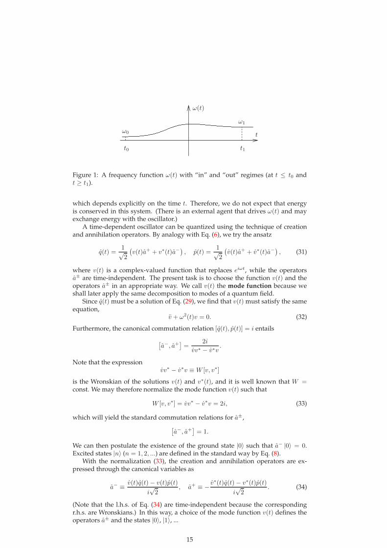
Figure 1: A frequency function ω(t) with “in” and “out” regimes (at t ≤ t0 andt ≥ t1).

which depends explicitly on the time t. Therefore, we do not expect that energyis conserved in this system. (There is an external agent that drives ω(t) and mayexchange energy with the oscillator.)

A time-dependent oscillator can be quantized using the technique of creationand annihilation operators. By analogy with Eq. (6), we try the ansatz

q(t) =1√2

(

v(t)a+ + v∗(t)a−)

, p(t) =1√2

(

v(t)a+ + v∗(t)a−)

, (31)

where v(t) is a complex-valued function that replaces eiωt, while the operatorsa± are time-independent. The present task is to choose the function v(t) and theoperators a± in an appropriate way. We call v(t) the mode function because weshall later apply the same decomposition to modes of a quantum field.

Since q(t) must be a solution of Eq. (29), we find that v(t) must satisfy the sameequation,

v + ω2(t)v = 0. (32)

Furthermore, the canonical commutation relation [q(t), p(t)] = i entails

[

a−, a+]

=2i

vv∗ − v∗v.

Note that the expressionvv∗ − v∗v ≡W [v, v∗]

is the Wronskian of the solutions v(t) and v∗(t), and it is well known that W =const. We may therefore normalize the mode function v(t) such that

W [v, v∗] = vv∗ − v∗v = 2i, (33)

which will yield the standard commutation relations for a±,

[

a−, a+]

= 1.

We can then postulate the existence of the ground state |0〉 such that a− |0〉 = 0.Excited states |n〉 (n = 1, 2, ...) are defined in the standard way by Eq. (8).

With the normalization (33), the creation and annihilation operators are ex-pressed through the canonical variables as

a− ≡ v(t)q(t) − v(t)p(t)

i√

2, a+ ≡ − v

∗(t)q(t) − v∗(t)p(t)

i√

2. (34)

(Note that the l.h.s. of Eq. (34) are time-independent because the correspondingr.h.s. are Wronskians.) In this way, a choice of the mode function v(t) defines theoperators a± and the states |0〉, |1〉, ...

15

It is clear that different choices of v(t) will in general define different operatorsa± and different states |0〉, |1〉, ... It is not clear, a priori, which choice of v(t) cor-responds to the “correct” ground state of the oscillator. The choice of v(t) will bestudied in the next section.

Properties of mode functionsHere is a summary of some elementary properties of a time-dependent oscillator

equationx+ ω2(t)x = 0. (35)

This equation has a two-dimensional space of solutions. Any two linearly independentsolutions x1(t) and x2(t) are a basis in that space. The expression

W [x1, x2] ≡ x1x2 − x1x2

is called the Wronskian of the two functions x1(t) and x2(t). It is easy to see thatthe Wronskian W [x1, x2] is time-independent if x1,2(t) satisfy Eq. (35). Moreover,W [x1, x2] 6= 0 if and only if x1(t) and x2(t) are two linearly independent solutions.

If x1(t), x2(t) is a basis of solutions, it is convenient to define the complex func-tion v(t) ≡ x1(t) + ix2(t). Then v(t) and v∗(t) are linearly independent and form abasis in the space of complex solutions of Eq. (35). It is easy to check that

Im(vv∗) =vv∗ − v∗v

2i=

1

2iW [v, v∗] = −W [x1, x2] 6= 0,

and thus the quantity Im(vv∗) is a nonzero real constant. If v(t) is multiplied by aconstant, v(t) → λv(t), the Wronskian W [v, v∗] changes by the factor |λ|2. Thereforewe may normalize v(t) to a prescribed value of Im(vv∗) by choosing the constant λ, aslong as v and v∗ are linearly independent solutions so that W [v, v∗] 6= 0.

A complex solution v(t) of Eq. (35) is an admissible mode function if v(t) is nor-malized by the condition Im(vv∗) = 1. It follows that any solution v(t) normalized byIm(vv∗) = 1 is necessarily complex-valued and such that v(t) and v∗(t) are a basis oflinearly independent complex solutions of Eq. (35).

4.2 Choice of mode function

We have seen that different choices of the mode function v(t) lead to different defi-nitions of the operators a± and thus to different “canditate ground states” |0〉. Thetrue ground state of the oscillator is the lowest-energy state and not merely somestate |0〉 satisfying a− |0〉 = 0, where a− is some arbitrary operator. Therefore we

may try to choose v(t) such that the mean energy 〈0| H |0〉 is minimized.For any choice of the mode function v(t), the Hamiltonian is expressed through

the operators a± as

H =|v|2 + ω2 |v|2

4

(

2a+a− + 1)

+v2 + ω2v2

4a+a+ +

v∗2 + ω2v∗2

4a−a−. (36)

Derivation of Eq. (36)In the canonical variables, the Hamiltonian is

H =1

2p2 +

1

2ω2(t)q2.

Now we expand the operators p, q through the mode functions using Eq. (31) and thecommutation relation

ˆ

a+, a−˜

= 1. For example, the term p2 gives

p2 =1√2

`

v(t)a+ + v∗(t)a−´ 1√

2

`

v(t)a+ + v∗(t)a−´

=1

2

`

v2a+a+ + vv∗`

2a+a− + 1´

+ v∗2a−a−´

.

16

The term q2 gives

q2 =1√2

`

v(t)a+ + v∗(t)a−´ 1√

2

`

v(t)a+ + v∗(t)a−´

=1

2

`

v2a+a+ + vv∗`

2a+a− + 1´

+ v∗2a−a−´

.

After some straightforward algebra we obtain the required result.

It is easy to see from Eq. (36) that the mean energy at time t is given by

E(t) ≡ 〈0| H(t) |0〉 =|v(t)|2 + ω2(t) |v(t)|2

4. (37)

We would like to find the mode function v(t) that minimizes the above quantity.Note that E(t) is time-dependent, so we may first try to minimize E(t0) at a fixedtime t0.

The choice of the mode function v(t) may be specified by a set of initial condi-tions at t = t0,

v(t0) = q, v(t0) = p,

where the parameters p and q are complex numbers satisfying the normalizationconstraint which follows from Eq. (33),

q∗p− p∗q = 2i. (38)

Now we need to find such p and q that minimize the expression |p|2 + ω2(t0) |q|2.This is a straightforward exercise (see below) which yields, for ω(t0) > 0, the fol-lowing result:

v(t0) =1

√

ω(t0), v(t0) = i

√

ω(t0) = iω(t0)v(t0). (39)

If, on the other hand, ω2(t0) < 0 (i.e. ω is imaginary), there is no minimum. Fornow, we shall assume that ω(t0) is real. Then the mode function satisfying Eq. (39)will define the operators a± and the state |t00〉 such that the instantaneous energyE(t0) has the lowest possible value Emin = 1

2ω(t0). The state |t00〉 is called theinstantaneous ground state at time t = t0.

Derivation of Eq. (39)If some p and q minimize |p|2 +ω2 |q|2, then so do eiλp and eiλq for arbitrary real λ;

this is the freedom of choosing the overall phase of the mode function. We may choosethis phase to make q real and write p = p1 + ip2 with real p1,2. Then Eq. (38) yields

q =2i

p− p∗=

1

p2⇒ 4E(t0) = p2

1 + p22 +

ω2(t0)

p22

. (40)

If ω2(t0) > 0, the function E (p1, p2) has a minimum with respect to p1,2 at p1 = 0 andp2 =

p

ω(t0). Therefore the desired initial conditions for the mode function are givenby Eq. (39).

On the other hand, if ω2(t0) < 0 the function Ek in Eq. (40) has no minimumbecause the expression p2

2 + ω2(t0)p−22 varies from −∞ to +∞. In that case the instan-

taneous lowest-energy ground state does not exist.

4.3 “In” and “out” states

Let us now consider the frequency function ω(t) shown in Fig. 1. It is easy to seethat the lowest-energy state is given by the mode function vin(t) = eiω0t in the“in” regime (t ≤ t0) and by vout(t) = eiω1t in the “out” regime (t ≥ t1). However,

17

note that vin(t) 6= eiω0t for t > t0; instead, vin(t) is a solution of Eq. (29) with theinitial conditions (39) at t = t0. Similarly, vout(t) 6= eiω1t for t < t1. While exactsolutions for vin(t) and vout(t) are in general not available, we may still analyze therelationship between these solutions in the “in” and “out” regimes.

Since the solutions e±iω1t are a basis in the space of solutions of Eq. (35), wemay write

vin(t) = αvout(t) + βv∗out(t), (41)

where α and β are time-independent constants. The relationship (41) between themode functions is an example of a Bogolyubov transformation (see Sec. 2.2). Us-ing Eq. (33) for vin(t) and vout(t), it is straightforward to derive the property

|α|2 − |β|2 = 1. (42)

For a general ω(t), we will have β 6= 0 and hence there will be no single modefunction v(t) matching both vin(t) and vout(t).

Each choice of the mode function v(t) defines the corresponding creation andannihilation operators a±. Let us denote by a±in the operators defined using themode function vin(t) and vout(t), respectively. It follows from Eqs. (34) and (41)that

a−in = αa−out − βa+out.

The inverse relation is easily found using Eq. (42),

a−out = α∗a−in + βa+in. (43)

Since generally β 6= 0, we cannot define a single set of operators a± which willdefine the ground state |0〉 for all times.

Moreover, in the intermediate regime where ω(t) is not constant, an instanta-neous ground state |t0〉 defined at time t will, in general, not be a ground state atthe next moment, t + ∆t. Therefore, such a state |t0〉 cannot be trusted as a phys-ically motivated ground state. However, if we restrict our attention only to the“in” regime, the mode function vin(t) defines a perfectly sensible ground state |0in〉which remains the ground state for all t ≤ t0. Similarly, the mode function vout(t)defines the ground state |0out〉.

Since we are using the Heisenberg picture, the quantum state |ψ〉 of the oscil-lator is time-independent. It is reasonable to plan the following experiment. Weprepare the oscillator in its ground state |ψ〉 = |0in〉 at some early time t < t0 withinthe “in” regime. Then we let the oscillator evolve until the time t = t1 and compareits quantum state (which remains |0in〉) with the true ground state, |0out〉, at timet > t1 within the “out” regime.

In the “out” regime, the state |0in〉 is not the ground state any more, and thus itmust be a superposition of the true ground state |0out〉 and the excited states |nout〉defined using the “out” creation operator a+

out,

|nout〉 =1√n!

(

a+out

)n |0out〉 , n = 0, 1, 2, ...

It can be easily verified that the vectors |nout〉 are eigenstates of the Hamiltonianfor t ≥ t1 (but not for t < t1):

H(t) |nout〉 = ω1

(

n+1

2

)

|nout〉 , t ≥ t1.

Similarly, the excited states |nin〉 may be defined through the creation operator a+in.

The states |nin〉 are interpreted as n-particle states of the oscillator for t ≤ t0, whilefor t ≥ t1 the n-particle states are |nout〉.

18

Remark: interpretation of the “in” and “out” states. We are presently working in theHeisenberg picture where quantum states are time-independent and operators dependon time. One may prepare the oscillator in a state |ψ〉, and the state of the oscillator re-mains the same throughout all time t. However, the physical interpretation of this statechanges with time because the state |ψ〉 is interpreted with help of the time-dependent

operators H(t), a−(t), etc. For instance, we found that at late times (t ≥ t1) the vector|0in〉 is not the lowest-energy state any more. This happens because the energy of thesystem changes with time due to the external force that drives ω(t). Without this force,we would have a−in = a−out and the state |0in〉 would describe the physical vacuum at alltimes.

4.4 Relationship between “in” and “out” states

The states |nout〉, where n = 0, 1, 2, ..., form a complete basis in the Hilbert spaceof the harmonic oscillator. However, the set of states |nin〉 is another completebasis in the same space. Therefore the vector |0in〉 must be expressible as a linearcombination of the “out” states,

|0in〉 =

∞∑

n=0

Λn |nout〉 , (44)

where Λn are suitable coefficients. If the mode functions are related by a Bo-golyubov transformation (41), one can show that these coefficients Λn are givenby

Λ2n =

[

1 −∣

∣

∣

∣

β

α

∣

∣

∣

∣

2]1/4

(

β

α

)n√

(2n− 1)!!

(2n)!!, Λ2n+1 = 0. (45)

The relation (44) shows that the early-time ground state is a superposition of

excited states at late times, having the probability |Λn|2 for the occupation numbern. We thus conclude that the presence of an external influence leads to excitationsof the oscillator. (Later on, when we consider field theory, such excitations will beinterpreted as particle production.) In the present case, the influence of externalforces on the oscillator consists of the changing frequency ω(t), which is formallya parameter of the Lagrangian. For this reason, the excitations arising in a time-dependent oscillator are called parametric excitations.

Finally, let us compute the expected particle number in the “out” regime, as-suming that the oscillator is in the state |0in〉. The expectation value of the number

operator Nout ≡ a+outa

−out in the state |0in〉 is easily found using Eq. (43):

〈0in| a+outa

−out |0in〉 = 〈0in|

(

αa+in + β∗a−in

) (

α∗a−in + βa+in

)

|0in〉 = |β|2 .

Therefore, a nonzero coefficient β signifies the presence of particles in the “out”region.

Derivation of Eq. (45)In order to find the coefficients Λn, we need to solve the equation

0 = a−in |0in〉 =`

αa−out − βa+out

´

∞X

n=0

Λn |nout〉 .

Using the known properties

a+ |n〉 =√n+ 1 |n+ 1〉 , a− |n〉 =

√n |n− 1〉 ,

we obtain the recurrence relation

Λn+2 = Λnβ

α

r

n+ 1

n+ 2; Λ1 = 0.

19

Therefore, only even-numbered Λ2n are nonzero and may be expressed through Λ0 asfollows,

Λ2n = Λ0

„

β

α

«ns

1 · 3 · ... · (2n− 1)

2 · 4 · ... · (2n)≡ Λ0

„

β

α

«ns

(2n− 1)!!

(2n)!!, n ≥ 1.

For convenience, one defines (−1)!! = 1, so the above expression remains valid also forn = 0.

The value of Λ0 is determined from the normalization condition, 〈0in| 0in〉 = 1,which can be rewritten as

|Λ0|2∞X

n=0

˛

˛

˛

˛

β

α

˛

˛

˛

˛

2n(2n− 1)!!

(2n)!!= 1.

The infinite sum can be evaluated as follows. Let f(z) be an auxiliary function definedby the series

f(z) ≡∞X

n=0

z2n (2n− 1)!!

(2n)!!.

At this point one can guess that this is a Taylor expansion of f(z) =`

1 − z2´−1/2

; then

one obtains Λ0 = 1/p

f(z) with z ≡ |β/α|. If we would like to avoid guessing, wecould manipulate the above series in order to derive a differential equation for f(z):

f(z) = 1 +

∞X

n=1

z2n 2n− 1

2n

(2n− 3)!!

(2n− 2)!!= 1 +

∞X

n=1

z2n (2n− 3)!!

(2n− 2)!!−

∞X

n=1

z2n

2n

(2n− 3)!!

(2n− 2)!!

= 1 + z2f(z) −∞X

n=1

z2n

2n

(2n− 3)!!

(2n− 2)!!.

Taking d/dz of both parts, we have

d

dz

ˆ

1 + z2f(z) − f(z)˜

=∞X

n=1

z2n−1 (2n− 3)!!

(2n− 2)!!= zf(z),

hence f(z) satisfies

d

dz

ˆ

(z2 − 1)f(z)˜

=`

z2 − 1´ df

dz+ 2zf(z) = zf(z); f(0) = 1.

The solution is

f(z) =1√

1 − z2.

Substituting z ≡ |β/α|, we obtain the required result,

Λ0 =

"

1 −˛

˛

˛

˛

β

α

˛

˛

˛

˛

2#1/4

.

4.5 Quantum-mechanical analogy

The time-dependent oscillator equation (35) is formally similar to the stationarySchrödinger equation for the wave function ψ(x) of a quantum particle in a one-dimensional potential V (x),

d2ψ

dx2+ (E − V (x))ψ = 0.

The two equations are related by the replacements t→ x and ω2(t) → E − V (x).

20

x1 x2

incoming

R

T

V (x)

x

Figure 2: Quantum-mechanical analogy: motion in a potential V (x).

To illustrate the analogy, let us consider the case when the potential V (x) isalmost constant for x < x1 and for x > x2 but varies in the intermediate region(see Fig. 2). An incident wave ψ(x) = exp(−ipx) comes from large positive x and isscattered off the potential. A reflected wave ψR(x) = R exp(ipx) is produced in theregion x > x2 and a transmitted wave ψT (x) = T exp(−ipx) in the region x < x1.For most potentials, the reflection amplitude R is nonzero. The conservation of

probability gives the constraint |R|2 + |T |2 = 1.The wavefunction ψ(x) behaves similarly to the mode function v(t) in the case

when ω(t) is approximately constant at t ≤ t0 and at t ≥ t1. If the wavefunctionrepresents a pure incoming wave x < x1, then at x > x2 the function ψ(x) willbe a superposition of positive and negative exponents exp (±ikx). This is the phe-nomenon known as over-barrier reflection: there is a small probability that theparticle is reflected by the potential, even though the energy is above the height ofthe barrier. The relation betweenR and T is similar to the normalization condition(42) for the Bogolyubov coefficients. The presence of the over-barrier reflection(R 6= 0) is analogous to the presence of particles in the “out” region (β 6= 0).

5 Scalar field in expanding universe

Let us now turn to the situation when quantum fields are influenced by stronggravitational fields. In this chapter, we use units where c = G = 1, where G isNewton’s constant.

5.1 Curved spacetime

Einstein’s theory of gravitation (General Relativity) is based on the notion ofcurved spacetime, i.e. a manifold with arbitrary coordinates x ≡ xµ and a met-ric gµν(x) which replaces the flat Minkowski metric ηµν . The metric defines theinterval

ds2 = gµνdxµdxν ,

which describes physically measured lengths and times. According to the Einsteinequation, the metric gµν(x) is determined by the distribution of matter in the entireuniverse.

Here are some basic examples of spacetimes. In the absence of matter, the met-ric is equal to the Minkowski metric ηµν = diag (1,−1,−1,−1) (in Cartesian coor-dinates). In the presence of a single black hole of massM , the metric can be writtenin spherical coordinates as

ds2 =

(

1 − 2M

r

)

dt2 −(

1 − 2M

r

)−1

dr2 − r2[

dθ2 + sin2 θdφ2]

.

21

Finally, a certain class of spatially homogeneous and isotropic distributions of mat-ter in the universe yields a metric of the form

ds2 = dt2 − a2(t)[

dx2 + dy2 + dy2]

, (46)

where a(t) is a certain function called the scale factor. (The interpretation is thata(t) “scales” the flat metric dx2 + dy2 + dz2 at different times.) Spacetimes withmetrics of the form (46) are called Friedmann-Robertson-Walker (FRW) spacetimeswith flat spatial sections (in short, flat FRW spacetimes). Note that it is only thethree-dimensional spatial sections which are flat; the four-dimensional geometry ofsuch spacetimes is usually curved. The class of flat FRW spacetimes is important incosmology because its geometry agrees to a good precision with the present resultsof astrophysical measurements.

In this course, we shall not be concerned with the task of obtaining the metric.It will be assumed that a metric gµν(x) is already known in some coordinates xµ.

5.2 Scalar field in cosmological background

Presently, we shall study the behavior of a quantum field in a flat FRW spacetimewith the metric (46). In Einstein’s General Relativity, every kind of energy influ-ences the geometry of spacetime. However, we shall treat the metric gµν(x) as fixedand disregard the influence of fields on the geometry.

A minimally coupled, free, real, massive scalar field φ(x) in a curved spacetimeis described by the action

S =

∫ √−gd4x

[

1

2gαβ (∂αφ) (∂βφ) − 1

2m2φ2

]

. (47)

(Note the difference between Eq. (47) and Eq. (11): the Minkowski metric ηµν isreplaced by the curved metric gµν , and the integration uses the covariant volumeelement

√−gd4x. This is the minimal change necessary to make the theory of thescalar field compatible with General Relativity.) The equation of motion for thefield φ is derived straightforwardly as

gµν∂µ∂νφ+1√−g (∂νφ) ∂µ

(

gµν√−g)

+m2φ = 0. (48)

This equation can be rewritten more concisely using the covariant derivative cor-responding to the metric gµν ,

gµν∇µ∇νφ+m2φ = 0,

which shows explicitly that this is a generalization of the Klein-Gordon equationto curved spacetime.

We cannot directly use the quantization technique developed for fields in theflat spacetime. First, let us carry out a few mathematical transformations to sim-plify the task.

The metric (46) for a flat FRW spacetime can be simplified if we replace thecoordinate t by the conformal time η,

η(t) ≡∫ t

t0

dt

a(t),

where t0 is an arbitrary constant. The scale factor a(t) must be expressed throughthe new variable η; let us denote that function again by a(η). In the coordinates(x, η), the interval is

ds2 = a2(η)[

dη2 − dx2]

, (49)

22

so the metric is conformally flat (equal to the flat metric multiplied by a factor):gµν = a2ηµν , gµν = a−2ηµν .

Further, it is convenient to introduce the auxiliary field χ ≡ a(η)φ. Then onecan show that the action (47) can be rewritten in terms of the field χ as follows,

S =1

2

∫

d3x dη(

χ′2 − (∇χ)2 −m2eff(η)χ

2)

, (50)

where the prime ′ denotes ∂/∂η, and meff is the time-dependent effective mass

m2eff(η) ≡ m2a2 − a′′

a. (51)

The action (50) is very similar to the action (11), except for the presence of thetime-dependent mass.

Derivation of Eq. (50)We start from Eq. (47). Using the metric (49), we have

√−g = a4 and gαβ = a−2ηαβ .Then

√−gm2φ2 = m2a2χ2,

√−g gαβφ,αφ,β = a2

`

φ′2 − (∇φ)2´

.

Substituting φ = χ/a, we get

a2φ′2 = χ′2 − 2χχ′ a′

a+ χ2

„

a′

a

«2

= χ′2 + χ2 a′′

a−»

χ2 a′

a

–′

.

The total time derivative term can be omitted from the action, and we obtain the re-quired expression.

Thus, the dynamics of a scalar field φ in a flat FRW spacetime is mathematicallyequivalent to the dynamics of the auxiliary field χ in the Minkowski spacetime. Allthe information about the influence of gravitation on the field φ is encapsulated inthe time-dependent mass meff(η) defined by Eq. (51). Note that the action (50) isexplicitly time-dependent, so the energy of the field χ is generally not conserved.We shall see that in quantum theory this leads to the possibility of particle creation;the energy for new particles is supplied by the gravitational field.

5.3 Mode expansion

It follows from the action (50) that the equation of motion for χ(x, η) is

χ′′ − ∆χ+

(

m2a2 − a′′

a

)

χ = 0. (52)

Expanding the field χ in Fourier modes,

χ (x, η) =

∫

d3k

(2π)3/2χk(η)eik·x, (53)

we obtain from Eq. (52) the decoupled equations of motion for the modes χk(η),

χ′′k

+

[

k2 +m2a2(η) − a′′

a

]

χk ≡ χ′′k

+ ω2k(η)χk = 0. (54)

All the modes χk(η) with equal |k| = k are complex solutions of the same equa-tion (54). This equation describes a harmonic oscillator with a time-dependentfrequency. Therefore, we may apply the techniques we developed in chapter 4.

23

We begin by choosing a mode function vk(η), which is a complex-valued solu-tion of

v′′k + ω2k(η)vk = 0, ω2

k(η) ≡ k2 +m2eff(η). (55)

Then, the general solution χk(η) is expressed as a linear combination of vk and v∗kas

χk(η) =1√2

[

a−kv∗k(η) + a+

−kvk(η)

]

, (56)

where a±k

are complex constants of integration that depend on the vector k (butnot on η). The index −k in the second term of Eq. (56) and the factor 1√

2are chosen

for later convenience.Since χ is real, we have χ∗

k= χ−k. It follows from Eq. (56) that a+

k=(

a−k

)∗.

Combining Eqs. (53) and (56), we find

χ (x, η) =

∫

d3k

(2π)3/2

1√2

[

a−kv∗k(η) + a+

−kvk(η)

]

eik·x

=

∫

d3k

(2π)3/2

1√2

[

a−kv∗k(η)eik·x + a+

kvk(η)e−ik·x] . (57)

Note that the integration variable k was changed (k → −k) in the second term ofEq. (57) to make the integrand a manifestly real expression. (This is done only forconvenience.)

The relation (57) is called the mode expansion of the field χ (x, η) w.r.t. themode functions vk(η). At this point the choice of the mode functions is still arbi-trary.

The coefficients a±k

are easily expressed through χk(η) and vk(η):

a−k

=√

2v′kχk − vkχ

′k

v′kv∗k − vkv∗′k

=√

2W [vk, χk]

W [vk, v∗k]; a+

k=(

a−k

)∗. (58)

Note that the numerators and denominators in Eq. (58) are time-independent sincethey are Wronskians of solutions of the same oscillator equation.

5.4 Quantization of scalar field

The field χ(x) can be quantized directly through the mode expansion (57), whichcan be used for quantum fields in the same way as for classical fields. The modeexpansion for the field operator χ is found by replacing the constants a±

kin Eq. (57)

by time-independent operators a±k

:

χ (x, η) =

∫

d3k

(2π)3/2

1√2

(

eik·xv∗k(η)a−k

+ e−ik·xvk(η)a+k

)

, (59)

where vk(η) are mode functions obeying Eq. (55). The operators a±k

satisfy theusual commutation relations for creation and annihilation operators,

[

a−k, a+

k′

]

= δ(k − k′),[

a−k, a−

k′

]

=[

a+k, a+

k′

]

= 0. (60)

The commutation relations (60) are consistent with the canonical relations

[χ(x1, η), χ′(x2, η)] = iδ(x1 − x2)

only if the mode functions vk(η) are normalized by the condition

Im (v′kv∗k) =

v′kv∗k − vkv

′∗k

2i≡ W [vk, v

∗k]

2i= 1. (61)

24

Therefore, quantization of the field χ can be accomplished by postulating the modeexpansion (59), the commutation relations (60) and the normalization (61). Thechoice of the mode functions vk(η) will be made later on.

The mode expansion (59) can be visualized as the general solution of the fieldequation (52), where the operators a±

kare integration constants. The mode expan-

sion can also be viewed as a definition of the operators a±k

through the field operatorχ (x, η). Explicit formulae relating a±

kto χ and π ≡ χ′ are analogous to Eq. (58).

Clearly, the definition of a±k

depends on the choice of the mode functions vk(η).

5.5 Vacuum state and particle states

Once the operators a±k

are determined, the vacuum state |0〉 is defined as the eigen-state of all annihilation operators a−

kwith eigenvalue 0, i.e. a−

k|0〉 = 0 for all k. An

excited state |mk1, nk2

, ...〉 with the occupation numbers m,n, ... in the modes χk1,

χk2, ..., is constructed by

|mk1, nk2

, ...〉 ≡ 1√m!n!...

[(

a+k1

)m (a+k2

)n...]

|0〉 . (62)

We write |0〉 instead of |0k1, 0k2

, ...〉 for brevity. An arbitrary quantum state |ψ〉 is alinear combination of these states,

|ψ〉 =∑

m,n,...

Cmn... |mk1, nk2

, ...〉 .

If the field is in the state |ψ〉, the probability for measuring the occupation number

m in the mode χk1, the number n in the mode χk2

, etc., is |Cmn...|2.Let us now comment on the role of the mode functions. Complex solutions

vk(η) of a second-order differential equation (55) with one normalization condi-tion (61) are parametrized by one complex parameter. Multiplying vk(η) by a con-stant phase eiα introduces an extra phase e±iα in the operators a±k , which can becompensated by a constant phase factor eiα in the state vectors |0〉 and |mk1

, nk2, ...〉.

There remains one real free parameter that distinguishes physically inequivalentmode functions. With each possible choice of the functions vk(η), the operators a±

k

and consequently the vacuum state and particle states are different. As long as themode functions satisfy Eqs. (55) and (61), the commutation relations (60) hold andthus the operators a±

kformally resemble the creation and annihilation operators for

particle states. However, we do not yet know whether the operators a±k

obtainedwith some choice of vk(η) actually correspond to physical particles and whetherthe quantum state |0〉 describes the physical vacuum. The correct commutationrelations alone do not guarantee the validity of the physical interpretation of theoperators a±

kand of the state |0〉. For this interpretation to be valid, the mode func-

tions must be appropriately selected; we postpone the consideration of this importantissue until Sec. 5.8 below. For now, we shall formally study the consequences ofchoosing several sets of mode functions to quantize the field φ.

5.6 Bogolyubov transformations

Suppose two sets of isotropic mode functions uk(η) and vk(η) are chosen. Since uk

and u∗k are a basis, the function vk is a linear combination of uk and u∗k, e.g.

v∗k(η) = αku∗k(η) + βkuk(η), (63)

with η-independent complex coefficients αk and βk. If both sets vk(η) and uk(η)are normalized by Eq. (61), it follows that the coefficients αk and βk satisfy

|αk|2 − |βk|2 = 1. (64)

25

In particular, |αk| ≥ 1.

Derivation of Eq. (64)We suppress the index k for brevity. The normalization condition for u(η) is

u∗u′ − uu′∗ = 2i.

Expressing u through v as given, we obtain`

|α|2 − |β|2´ `

v∗v′ − vv′∗´

= 2i.

The formula (64) follows from the normalization of v(η).

Using the mode functions uk(η) instead of vk (η), one obtains an alternative

mode expansion which defines another set b±k

of creation and annihilation opera-tors,

χ (x, η) =

∫

d3k

(2π)3/2

1√2

(

eik·xu∗k(η)b−k

+ e−ik·xuk(η)b+k

)

. (65)

The expansions (59) and (65) express the same field χ (x, η) through two differentsets of functions, so the k-th Fourier components of these expansions must agree,

eik·x[

u∗k(η)b−k

+ uk(η)b+−k

]

= eik·x [v∗k(η)a−k

+ vk(η)a+−k

]

.

A substitution of vk through uk using Eq. (63) gives the following relation between

the operators b±k

and a±k

:

b−k

= αka−k

+ β∗k a

+−k, b+

k= α∗

ka+k

+ βka−−k. (66)

The relation (66) and the complex coefficients αk, βk are called respectively theBogolyubov transformation and the Bogolyubov coefficients.6

The two sets of annihilation operators a−k

and b−k

define the correspondingvacua

∣

∣

(a)0⟩

and∣

∣

(b)0⟩

, which we call the “a-vacuum” and the “b-vacuum.” Twoparallel sets of excited states are built from the two vacua using Eq. (62). We referto these states as a-particle and b-particle states. So far the physical interpretationof the a- and b-particles remains unspecified. Later on, we shall apply this for-malism to study specific physical effects and the interpretation of excited statescorresponding to various mode functions will be explained. At this point, let usonly remark that the b-vacuum is in general a superposition of a-states, similarlyto what we found in Sec. 4.4.

5.7 Mean particle number

Let us calculate the mean number of b-particles of the mode χk in the a-vacuum

state. The expectation value of the b-particle number operator N(b)k

= b+kb−k

in thestate

∣

∣

(a)0⟩

is found using Eq. (66):

⟨

(a)0∣

∣ N (b)∣

∣

(a)0⟩

=⟨

(a)0∣

∣ b+kb−k

∣

∣

(a)0⟩

=⟨

(a)0∣

∣

(

α∗ka

+k

+ βka−−k

) (

αka−k

+ β∗k a

+−k

) ∣

∣

(a)0⟩

=⟨

(a)0∣

∣

(

βka−−k

) (

β∗k a

+−k

)∣

∣

(a)0⟩

= |βk|2 δ(3)(0). (67)

The divergent factor δ(3)(0) is a consequence of considering an infinite spatial vol-ume. This divergent factor would be replaced by the box volume V if we quantizedthe field in a finite box. Therefore we can divide by this factor and obtain the meandensity of b-particles in the mode χk,

nk = |βk|2 . (68)

6The pronunciation is close to the American “bogo-lube-of” with the third syllable stressed.

26

The Bogolyubov coefficient βk is dimensionless and the density nk is the meannumber of particles per spatial volume d3x and per wave number d3k, so that∫

nkd3k d3x is the (dimensionless) total mean number of b-particles in the a-vacuum

state.The combined mean density of particles in all modes is

∫

d3k |βk|2. Note thatthis integral might diverge, which would indicate that one cannot disregard thebackreaction of the produced particles on other fields and on the metric.

5.8 Instantaneous lowest-energy vacuum

In the theory developed so far, the particle interpretation depends on the choiceof the mode functions. For instance, the a-vacuum

∣

∣

(a)0⟩

defined above is a statewithout a-particles but with b-particle density nk in each mode χk. A natural ques-tion to ask is whether the a-particles or the b-particles are the correct representationof the observable particles. The problem at hand is to determine the mode func-tions that describe the “actual” physical vacuum and particles.

Previously, we defined the vacuum state as the eigenstate with the lowest en-ergy. However, in the present case the Hamiltonian explicitly depends on timeand thus does not have time-independent eigenstates that could serve as vacuumstates.

One possible prescription for the vacuum state is to select a particular momentof time, η = η0, and to define the vacuum |η0

0〉 as the lowest-energy eigenstate of

the instantaneous Hamiltonian H(η0). To obtain the mode functions that describethe vacuum |η0

0〉, we first compute the expectation value⟨

(v)0∣

∣ H(η0)∣

∣

(v)0⟩

in the

vacuum state∣

∣

(v)0⟩

determined by arbitrarily chosen mode functions vk(η). Thenwe can minimize that expectation value with respect to all possible choices of vk(η).

(A standard result in linear algebra is that the minimization of 〈x| A |x〉 with respectto all normalized vectors |x〉 is equivalent to finding the eigenvector |x〉 of the

operator A with the smallest eigenvalue.) This computation is analogous to thatof Sec. 4.2, and the result is similar to Eq. (39): If ω2

k(η0) > 0, the required initialconditions for the mode functions are

vk (η0) =1

√

ωk(η0), v′k(η0) = i

√

ωk(η0) = iωkvk(η0). (69)

If ω2k(η0) < 0, the instantaneous lowest-energy vacuum state does not exist.For a scalar field in the Minkowski spacetime, ωk is time-independent and the

prescription (69) yields the standard mode functions

vk(η) =1√ωkeiωkη,

which remain the vacuum mode functions at all times. But this is not the casefor a time-dependent gravitational background, because then ωk(η) 6= const andthe mode function selected by the initial conditions (69) imposed at a time η0 willgenerally differ from the mode function selected at another time η1 6= η0. In otherwords, the state |η0

0〉 is not an energy eigenstate at time η1. In fact, one can showthat there are no states which remain instantaneous eigenstates of the Hamiltonianat all times.

5.9 Computation of Bogolyubov coefficients

Computations of Bogolyubov coefficients requires knowledge of solutions of Eq. (55),which is an equation of a harmonic oscillator with a time-dependent frequency,

27

with specified initial conditions. Suppose that vk(η) and uk(η) are mode functionsdescribing instantaneous lowest-energy states defined at times η = η0 and η = η1.To determine the Bogolyubov coefficients αk and βk connecting these mode func-tions, it is necessary to know the functions vk(η) and uk(η) and their derivatives atonly one value of η, e.g. at η = η0. From Eq. (63) and its derivative at η = η0, wefind

v∗k (η0) = αku∗k (η0) + βkuk (η0) ,

v∗′k (η0) = αku∗′k (η0) + βku

′k (η0) .

This system of equations can be solved for αk and βk using Eq. (61):

αk =u′kv

∗k − ukv

∗′k

2i

∣

∣

∣

∣

η0

, β∗k =

u′kvk − ukv′k

2i

∣

∣

∣

∣

η0

. (70)

These relations hold at any time η0 (note that the numerators are Wronskians andthus are time-independent). For instance, knowing only the asymptotics of vk(η)and uk(η) at η → −∞ would suffice to compute αk and βk.

A well-known method to obtain an approximate solution of equations of thetype (55) is the WKB approximation, which gives the approximate solution satis-fying the condition (69) at time η = η0 as

vk(η) ≈ 1√

ωk(η)exp

[

i

∫ η

η0

ωk(η1)dη1

]

. (71)

However, it is straightforward to see that the approximation (71) satisfies the in-stantaneous minimum-energy condition at every other time η 6= η0 as well. Inother words, within the WKB approximation, uk(η) ≈ vk(η). Therefore, if we usethe WKB approximation to compute the Bogolyubov coefficient between instan-taneous vacuum states, we shall obtain the incorrect result βk = 0. The WKBapproximation is insufficiently precise to capture the difference between the in-stantaneous vacuum states defined at different times.

One can use the following method to obtain a better approximation to the modefunction vk(η). Let us focus attention on one mode and drop the index k. Introducea new variable Z(η) instead of v(η) as follows,

v(η) =1

√

ω(η0)exp

[

i

∫ η

η0

ω(η1)dη1 +

∫ η

η0

Z(η1)dη1

]

;v′

v= iω(η) + Z(η).

If ω(η) is a slow-changing function, then we expect that v(η) is everywhere approx-imately equal to 1√

ωexp

[

i∫ η

ω(η)dη]

and the function Z(η) under the exponential

is a small correction; in particular, Z(η0) = 0 at the time η0. It is straightforward toderive the equation for Z(η) from Eq. (55),

Z ′ + 2iωZ = −iω′ − Z2.

This equation can be solved using perturbation theory by treating Z2 as a smallperturbation. To obtain the first approximation, we disregard Z2 and straightfor-wardly solve the resulting linear equation, which yields

Z(1)(η) = −i∫ η

η0

dη1ω′(η1) exp

[

−2i

∫ η

η1

ω(η2)dη2

]

.

Note that Z(1)(η) is an integral of a slow-changing function ω′(η) multiplied bya quickly oscillating function and is therefore small, |Z| ≪ ω. The first approxi-mation Z(1) is sufficiently precise in most cases. The resulting approximate mode

28

function is

v(η) ≈ 1√

ω(η0)exp

[

i

∫ η

η0

ω(η1)dη1 +

∫ η

η0

Z(1)(η)dη

]

.

The Bogolyubov coefficient β between instantaneous lowest-energy states definedat times η0 and η1 can be approximately computed using Eq. (70):

u(η1) =1

√

ω(η1); u′(η1) = iω(η1)u(η1);

β∗ =1

2i√

ω(η1)[iω(η1)v(η1) − v′(η1)] = v(η1)

(

iω − v′

v

)

η1

2i√

ω(η1)≈ −v(η1)Z(η1)

2i√

ω(η1).

Since v(η1) is of orderω−1/2 and |Z| ≪ ω, the number of particles is small: |β|2 ≪ 1.

6 Amplitude of quantum fluctuations

In the previous chapter the focus was on particle production. The main observ-

able of interest was the average particle number 〈N〉. Now we consider anotherimportant quantity—the amplitude of field fluctuations.

6.1 Fluctuations of averaged fields

The value of a field cannot be observed at a mathematical point in space. Realis-tic devices can only measure the value of the field averaged over some region ofspace. Spatial averages are also the relevant quantity in cosmology because struc-ture formation in the universe is explained by fluctuations occurring over largeregions, e.g. of galaxy size. Therefore, let us consider values of fields averagedover a spatial domain.

A convenient way to describe spatial averaging over arbitrary domains is byusing window functions. A window function for scale L is any function W (x)which is of order 1 for |x| . L, rapidly decays for |x| ≫ L, and satisfies the nor-malization condition

∫

W (x) d3x = 1. (72)

A typical example of a window function is the spherical Gaussian window

WL (x) =1

(2π)3/2L3exp

[

−|x|22L2

]

,

which selects |x| . L. This window can be used to describe measurements per-formed by a device that cannot resolve distances smaller than L.

We define the averaged field operator χL(η) by integrating the product of χ(x, η)with a window function that selects the scale L,

χL(η) ≡∫

d3x χ (x, η)WL(x),

where we used the Gaussian window (although the final result will not depend onthis choice). The amplitude δχL(η) of fluctuations in χL(η) in a quantum state |ψ〉is found from

δχ2L(η) ≡ 〈ψ| [χL(η)]

2 |ψ〉 .

29

For simplicity, we consider the vacuum state |ψ〉 = |0〉. Then the amplitude ofvacuum fluctuations in χL(η) can be computed as a function ofL. We use the modeexpansion (59) for the field operator χ(x, η), assuming that the mode functionsvk(η) are given. After some straightforward algebra we find

〈0|[∫

d3xWL(x)χ (x, η)

]2

|0〉 =1

2

∫

d3k

(2π)3|vk|2 e−k2L2

.

Since the factor e−k2L2

is of order 1 for |k| . L−1 and almost zero for |k| & L−1,we can estimate the above integral as follows,

1

2

∫

d3k

(2π)3|vk|2 e−k2L2 ∼

∫ L−1

0

k2 |vk|2 dk ∼ k3 |vk|2∣

∣

∣

k=L−1

.

Thus the amplitude of fluctuations δχL is (up to a factor of order 1)

δχ2L ∼ k3 |vk|2 , where k ∼ L−1. (73)

The result (73) is (for any choice of the window function WL) an order-of-magnitude estimate of the amplitude of fluctuations on scale L. This quantity,which we denote by δχL(η), is defined only up to a factor of order 1 and is a func-tion of time η and of the scale L. Expressed through the wavenumber k ≡ 2πL−1,the fluctuation amplitude is usually called the spectrum of fluctuations.

6.2 Fluctuations in Minkowski spacetime

Let us now compute the spectrum of fluctuations for a scalar field in the Minkowskispace.

The vacuum mode functions are vk(η) = ω−1/2k exp (iωkη), whereωk =

√k2 +m2.

Thus, the spectrum of fluctuations in vacuum is

δχL(η) = k3/2 |vk(η)| =k3/2

(k2 +m2)1/4

. (74)

This time-independent spectrum is sketched in Fig. 3. When measured with ahigh-resolution device (small L), the field shows large fluctuations. On the otherhand, if the field is averaged over a large volume (L → ∞), the amplitude offluctuations tends to zero.

6.3 de Sitter spacetime

The de Sitter spacetime is used in cosmology to describe periods of acceleratedexpansion of the universe. The amplitude of fluctuations is an important quantityto compute in that context.

The geometry of the de Sitter spacetime may be specified by a flat FRW metric

ds2 = dt2 − a2(t)dx2 (75)

with the scale factor a(t) defined by

a(t) = a0eHt. (76)

The Hubble parameter H = a/a > 0 is a fixed constant. For convenience, weredefine the origin of time t to set a0 = 1, so that a(t) = exp(Ht). The exponen-tially growing scale factor describes an accelerating expansion (inflation) of theuniverse.

30

δχ

k

∼ k

∼ k3/2

Figure 3: A sketch of the spectrum of fluctuations δχL in the Minkowski space;L ≡ 2πk−1. (The logarithmic scaling is used for both axes.)

Horizons

An important feature of the de Sitter spacetime—the presence of horizons—is re-vealed by the following consideration of trajectories of lightrays. A null worldlinex(t) satisfies a2(t)x2(t) = 1, which yields the solution

|x(t)| =1

H

(

e−Ht0 − e−Ht)

for trajectories starting at the origin, x(t0) = 0. Therefore all lightrays emitted atthe origin at t = t0 asymptotically approach the sphere

|x| = rmax(t0) ≡ H−1 exp(−Ht0) = (aH)−1.

This sphere is the horizon for the observer at the origin; the spacetime expands tooquickly for lightrays to reach any points beyond the horizon. Similarly, observersat the origin will never receive any lightrays emitted at t = t0 at points |x| > rmax.

It is easy to verify that at any time t0 the horizon is always at the same properdistance a(t0)rmax(t0) = H−1 from the observer. This distance is called the horizonscale.

6.4 Quantum fields in de Sitter spacetime

To describe a real scalar field φ (x, t) in the de Sitter spacetime, we first transformthe coordinate t to make the metric explicitly conformally flat:

ds2 = dt2 − a2(t)dx2 = a2(η)(

dη2 − dx2)

,

where the conformal time η and the scale factor a(η) are

η = − 1

He−Ht, a(η) = − 1

Hη.

The conformal time η changes from −∞ to 0 when the proper time t goes from−∞ to +∞. (Since the value of η is always negative, we shall sometimes have towrite |η| in the equations. However, it is essential that the variable η grows whent grows, so we cannot use −η as the time variable. For convenience, we chose theorigin of η so that the infinite future corresponds to η = 0.)

31

The field φ(x, η) can now be quantized by the method of Sec. 2.2. We introducethe auxiliary field χ ≡ aφ and use the mode expansion (59)-(55) with

ω2k(η) = k2 +m2a2 − a′′

a= k2 +

(

m2

H2− 2

)

1

η2. (77)

From this expression it is clear that the effective frequency may become imaginary,i.e. ω2

k(η) < 0, if m2 < 2H2. In most cosmological scenarios where the early uni-verse is approximated by a region of the de Sitter spacetime, the relevant value ofH is much larger than the masses of elementary particles, i.e. m ≪ H . Therefore,for simplicity we shall consider the massless field.

6.5 Bunch-Davies vacuum state

As we saw before, the vacuum state of a field is determined by the choice of modefunctions. Let us now find the appropriate mode functions for a scalar field in deSitter spacetime.

With the definition (77) of the effective frequency, where we set m = 0, Eq. (55)becomes

v′′k +

(

k2 − 2

η2

)

vk = 0. (78)

The general solution of Eq. (78) can be written as

vk(η) = Ak

(

1 +i

kη

)

eikη +Bk

(

1 − i

kη

)

e−ikη, (79)

where Ak and Bk are constants. It is straightforward to check that the normal-ization of the mode function, Im (v∗kv

′k) = 1, constrains the constants Ak and Bk

by

|Ak|2 − |Bk| =1

k.

The constants Ak, Bk determine the mode functions and must be chosen ap-propriately to obtain a physically motivated vacuum state. For fields in de Sitterspacetime, there is a preferred vacuum state, which is known as the Bunch-Davies(BD) vacuum. This state is defined essentially as the Minkowski vacuum in theearly-time limit (η → −∞) of each mode.

Before introducing the BD vacuum, let us consider the prescription of the in-stantaneous vacuum defined at a time η = η0. If we had ω2

k(η0) > 0 for all k, thisprescription would yield a well-defined vacuum state. However, there always ex-ists a small enough k such that k |η0| ≪ 1 and thus ω2

k(η0) < 0. We have seen thatthe energy in a mode χk cannot be minimized when ω2

k < 0. Therefore the instan-taneous energy prescription cannot define a vacuum state of the entire quantumfield (for all modes) but only for the modes χk with k |η0| & 1. Note that these arethe modes whose wavelength was shorter than the horizon length, (aH)−1 = |η0|,at time η0 (i.e. the subhorizon modes).

The motivation for introducing the BD vacuum state is the following. The effec-tive frequency ωk(η) becomes constant in the early-time limit η → −∞. Physically,this means that the influence of gravity on each mode χk is negligible at sufficientlyearly (k-dependent) times. When gravity is negligible, there is a unique vacuumprescription—the Minkowski vacuum, which coincides with the instantaneousminimum-energy vacuum at all times. So it is natural to define the mode func-tions vk(η) by applying the Minkowski vacuum prescription in the limit η → −∞,separately for each mode χk. This prescription can be expressed by the asymptoticrelations

vk(η) → 1√ωkeiωkη,

v′k(η)

vk(η)→ iωk, as η → −∞. (80)

32

The vacuum state determined by the mode functions vk(η) satisfying Eq. (80) iscalled the Bunch-Davies vacuum. It follows that the mode functions of the BDvacuum are given by Eq. (79) with Ak = 1/

√k and Bk = 0, namely

vk(η) =1√k

(

1 +i

kη

)

eikη. (81)

The Bunch-Davies vacuum prescription has important applications in cosmol-ogy where the de Sitter spacetime approximates the inflationary stage of the evo-lution of the universe. However, this approximation is valid only for a certain timeinterval, for instance ηi < η < ηf , while at earlier times, η < ηi, the spacetime is notde Sitter. Therefore the procedure of imposing the minimum-energy conditions atearlier times η < ηi cannot be justified, and the BD vacuum state can be used onlyfor modes χk such that k |ηi| ≫ 1. However, it is these modes that are importantfor cosmological predictions.

6.6 Spectrum of fluctuations in the BD vacuum

Let us now compute the fluctuation amplitude δφL(η) in the BD vacuum state andcompare the result with the fluctuations in Minkowski spacetime.

According to the formula (73), the amplitude of fluctuations is determined byabsolute values of the mode functions. Up to now we have been mostly working

with the auxiliary field χ(x) = aφ(x). The mode expansion for φ(x) is simplya−1(η) times the mode expansion for χ. Therefore, the mode functions of the field

φ are a−1(η)vk(η), where vk(η) are the mode functions of the field χ. Hence, the

spectrum of fluctuations of φ is

δφL(η) = a−1(η)k3/2 |vk(η)| = H√

k2η2 + 1. (82)

This spectrum is to be compared with Eq. (74) with m = 0. The spectrum (82) forearly times (|η| ≫ k) is the same as in the Minkowski spacetime, while for late

times or for superhorizon scales (k ≪ |η|−1) the spectrum (82) becomes almost

independent of k (scale-invariant) and shows much larger fluctuations than thespectrum (74). The growth of fluctuations is due to the influence of gravity on the

field φ.The growth of quantum fluctuations is used in cosmology to explain the for-

mation of large-scale structures (galaxies and clusters of galaxies) in the early uni-verse. The theory of cosmological inflation assumes the existence of a de Sitter-likeepoch in the history of the universe. During this epoch, vacuum fluctuations of thefields were significantly amplified. The resulting large quantum fluctuations actedas seeds for the inhomogeneities of energy density, which then grew by gravita-tional collapse and eventually caused the formation of galaxies. This theory is apractical application of quantum field theory in curved spacetime to astrophysics.

7 Unruh effect

The Unruh effect predicts that particles will be detected in a vacuum by an acceler-ated observer. In this chapter we consider the simplest case, in which the observermoves with constant acceleration through Minkowski spacetime and measures thenumber of particles in a massless scalar field. Even though the field is in the vac-uum state, the observer finds a distribution of particles characteristic of a thermalbath of blackbody radiation.

33

7.1 Kinematics of uniformly accelerated motion

First we consider the trajectory of an object moving with constant acceleration inthe Minkowski spacetime. A model of this situation is a spaceship with an infiniteenergy supply and a propulsion engine that exerts a constant force (but moves withthe ship). The resulting motion of the spaceship is such that the acceleration of theship in its own frame of reference (the proper acceleration) is constant. This is thenatural definition of a uniformly accelerated motion in a relativistic theory. (Anobject cannot move with dv/dt = const for all time because its velocity is alwayssmaller than the speed of light, |v| < 1.)

We now introduce the reference frames that will play a major role in our consid-erations: the laboratory frame, the proper frame, and the comoving frame. The lab-oratory frame is the usual inertial reference frame with the coordinates (t, x, y, z).The proper frame is the accelerated system of reference that moves together withthe observer; we shall also call it the accelerated frame. The comoving frame de-fined at a time t0 is the inertial frame in which the accelerated observer is instan-taneously at rest at t = t0. (Thus the term comoving frame actually refers to adifferent frame for each t0.)

By definition, the observer’s proper acceleration at time t = t0 is the 3-accelerationmeasured in the comoving frame at time t0. We consider a uniformly acceleratedobserver whose proper acceleration is time-independent and equal to a given 3-vector a. The trajectory of such an observer may be described by a worldlinexµ(τ), where τ is the proper time measured by the observer. The proper timeparametrization implies the condition

uµuµ = 1, uµ ≡ dxµ

dτ. (83)

It is a standard result that the 4-acceleration in the laboratory frame,

aµ ≡ duµ

dτ=d2xµ

dτ2,

is related to the three-dimensional proper acceleration a by

aµaµ = − |a|2 . (84)

Derivation of Eq. (84). Let uµ(τ ) be the observer’s 4-velocity and let tc be the timevariable in the comoving frame defined at τ = τ0; this is the time measured by aninertial observer moving with the constant velocity uµ(τ0). We shall show that the 4-acceleration aµ(τ ) in the comoving frame has components

`

0, a1, a2, a3´

, where ai arethe components of the acceleration 3-vector a ≡ d2

x/dt2c measured in the comovingframe. It will then follow that Eq. (84) holds in the comoving frame, and hence it holdsalso in the laboratory frame since the Lorentz-invariant quantity aµaµ is the same in allframes.

Since the comoving frame moves with the velocity uµ(τ0), the 4-vector uµ(τ0) hasthe components (1, 0, 0, 0) in that frame. The derivative of the identity uµ(τ )uµ(τ ) = 1with respect to τ yields aµ(τ )uµ(τ ) = 0, therefore a0(τ0) = 0 in the comoving frame.Since dtc = u0(τ )dτ and u0(τ0) = 1, we have

d2xµ

dt2c=

1

u0

d

dτ

»

1

u0

dxµ

dτ

–

=d2xµ

dτ 2+dxµ

dτ

d

dτ

1

u0.

It remains to compute

d

dτ

1

u0(τ0)= −

ˆ

u0(τ0)˜−2 du0

dτ

˛

˛

˛

˛

τ=τ0

= −a0 (τ0) = 0,

34

and it follows that d2xµ/dτ 2 = d2xµ/dt2c =`

0, a1, a2, a3´

as required. (Self-test ques-tion: why is aµ = duµ/dτ 6= 0 even though uµ = (1, 0, 0, 0) in the comoving frame?)

We now derive the trajectory xµ(τ) of the accelerated observer. Without lossof generality, we may assume that the acceleration is parallel to the x axis, a ≡(a, 0, 0), where a > 0, and that the observer moves only in the x direction. Thenthe coordinates y and z of the observer remain constant and only the functionsx(τ), t(τ) need to be computed. From Eqs. (83)-(84) it is straightforward to derivethe general solution

x(τ) = x0 −1

a+

1

acoshaτ, t(τ) = t0 +

1

asinh aτ. (85)

This trajectory has zero velocity at τ = 0 (which implies x = x0, t = t0).

Derivation of Eq. (85). Since aµ = duµ/dτ and u2 = u3 = 0, the components u0, u1 ofthe velocity satisfy

„

du0

dτ

«2

−„

du1

dτ

«2

= −a2,

`

u0´2 −

`

u1´2

= 1.

We may assume that u0 > 0 (the time τ grows together with t) and that du1/dτ > 0,since the acceleration is in the positive x direction. Then

u0 =

q

1 + (u1)2;du1

dτ= a

q

1 + (u1)2.

The solution with the initial condition u1(0) = 0 is

u1(τ ) ≡ dx

dτ= sinh aτ, u0(τ ) ≡ dt

dτ= cosh aτ.

After an integration we obtain Eq. (85).

The trajectory (85) has a simpler form if we choose the initial conditions x(0) =a−1 and t(0) = 0. Then the worldline is a branch of the hyperbola x2−t2 = a−2 (seeFig. 4). At large |t| the worldline approaches the lightcone. The observer comes infrom x = +∞, decelerates and stops at x = a−1, and then accelerates back towardsinfinity. In the comoving frame of the observer, this motion takes infinite propertime, from τ = −∞ to τ = +∞.

From now on, we drop the coordinates y and z and work in the 1+1-dimensionalspacetime (t, x).

7.2 Coordinates in the proper frame

To describe quantum fields as seen by an accelerated observer, we need to use theproper coordinates (τ, ξ), where τ is the proper time and ξ is the distance measuredby the observer. The proper coordinate system (τ, ξ) is related to the laboratoryframe (t, x) by some transformation functions τ(t, x) and ξ(t, x) which we shallnow determine.

The observer’s trajectory t(τ), x(τ) should correspond to the line ξ = 0 in theproper coordinates. Let the observer hold a rigid measuring stick of proper lengthξ0, so that the entire stick accelerates together with the observer. Then the stick isinstantaneously at rest in the comoving frame and the far endpoint of the stick hasthe proper coordinates (τ, ξ0) at time τ . We shall derive the relation between thecoordinates (t, x) and (τ, ξ) by computing the laboratory coordinates (t, x) of thefar end of the stick as functions of τ and ξ0.

35

Q

P

R

a−1

t = −x

t =x

x

t

0

Figure 4: The worldline of a uniformly accelerated observer (proper accelerationa ≡ |a|) in the Minkowski spacetime. The dashed lines show the lightcone. Theobserver cannot receive any signals from the events P , Q and cannot send signalsto R.

36

In the comoving frame at time τ , the stick is represented by the 4-vector sµ(com) ≡

(0, ξ0) connecting the endpoints (τ, 0) and (τ, ξ0). This comoving frame is an iner-tial system of reference moving with the 4-velocity uµ(τ) = dxµ/dτ . Therefore thecoordinates sµ

(lab) of the stick in the laboratory frame can be found by applying the

inverse Lorentz transformation to the coordinates sµ(com):

[

s0(lab)

s1(lab)

]

=1√

1 − v2

(

1 vv 1

)

[

s0(com)

s1(com)

]

=

(

u0 u1

u1 u0

)

[

s0(com)

s1(com)

]

=

[

u1ξu0ξ

]

,

where v ≡ u1/u0 is the velocity of the stick in the laboratory system. The stick isattached to the observer moving along xµ(τ), so the proper coordinates (τ, ξ) ofthe far end of the stick correspond to the laboratory coordinates

t(τ, ξ) = x0(τ) + s0(lab) = x0(τ) +dx1(τ)

dτξ, (86)

x(τ, ξ) = x1(τ) + s1(lab) = x1(τ) +dx0(τ)

dτξ. (87)

Note that the relations (86)-(87) specify the proper frame for any trajectory x0,1(τ)in the 1+1-dimensional Minkowski spacetime.

Now we can substitute Eq. (85) into the above relations to compute the propercoordinates for a uniformly accelerated observer. We choose the initial conditionsx0(0) = 0, x1(0) = a−1 for the observer’s trajectory and obtain

t(τ, ξ) =1 + aξ

asinh aτ, x(τ, ξ) =

1 + aξ

acoshaτ. (88)

The converse relations are

τ(t, x) =1

2alnx+ t

x− t, ξ(t, x) = −a−1 +

√

x2 − t2.

The horizon

It can be seen from Eq. (88) that the coordinates (τ, ξ) vary in the intervals −∞ <τ < +∞ and −a−1 < ξ < +∞. In particular, for ξ < −a−1 we would find∂t/∂τ < 0, i.e. the direction of time t would be opposite to that of τ . One canverify that an accelerated observer cannot measure distances longer than a−1 inthe direction opposite to the acceleration, for instance, the distances to the eventsP and Q in Fig. 4. A measurement of the distance to a point requires to place aclock at that point and to synchronize that clock with the observer’s clock. How-ever, the observer cannot synchronize clocks with the events P and Q because nosignals can be ever received from these events. One says that the accelerated ob-server perceives a horizon at proper distance a−1.

The existence of the horizon can be easily seen by the following qualitativeconsiderations. The accelerated observer measures a constant gravitational fieldwith acceleration a pointing in the negative x direction. Consider a photon ofenergy E propagating “upwards” in the gravitational field. After ascending to aheight ∆h, the photon loses energy, ∆E = −Ea∆h. After ascending to the height∆h = a−1, the photon would lose all its kinetic energy and will not be able tocontinue moving upwards. (This calculation is of course not rigorous but doesgive the correct answer.)

The coordinate system (88) is incomplete and covers only a “quarter” of theMinkowski spacetime, consisting of the subdomain x > |t| (see Fig. 5). This isthe subdomain of the Minkowski spacetime accessible to a uniformly accelerated

37

observer. For instance, the events P , Q, R cannot be described by (real) values of τand ξ. The past lightcone x = −t corresponds to the proper coordinates τ = −∞and ξ = −a−1. The observer can see signals from the event R, however these sig-nals appear to have originated not from R but from the horizon ξ = −a−1 in theinfinite past τ = −∞.

Another way to see that the line ξ = −a−1 is a horizon is to consider a line ofconstant proper length ξ = ξ0 > −a−1. It follows from Eq. (88) that the line ξ = ξ0is a trajectory of the form x2 − t2 = const with the proper acceleration

a0 ≡ 1√x2 − t2

=(

ξ0 + a−1)−1

.

Therefore, the worldline ξ = −a−1 would have to represent an infinite properacceleration, which would require an infinitely large force and is thus impossible.It follows that an accelerated observer cannot hold a rigid measuring stick longerthan a−1 in the direction opposite to acceleration. (A rigid stick is one that wouldkeep its proper distance constant in the observer’s reference frame.)

7.3 Rindler spacetime

It is straightforward to show that the Minkowski metric in the proper coordinates(τ, ξ) is

ds2 = dt2 − dx2 = (1 + aξ)2dτ2 − dξ2. (89)

The spacetime with this metric is called the Rindler spacetime. The curvature of theRindler spacetime is everywhere zero since it differs from the Minkowski space-time merely by a change of coordinates.

To develop the quantum field theory in the Rindler spacetime, we first rewritethe metric (89) in a conformally flat form. This can be achieved by choosing the

new spatial coordinate ξ such that dξ = (1 + aξ)dξ, because in that case both dτ2

and dξ2 will have a common factor (1 + aξ)2. (Note that the new coordinate ξ isa “conformal distance” fully analogous to the “conformal time” variable η used inSec. 5.4.) The necessary replacement is therefore

ξ ≡ 1

aln(1 + aξ).

Since the proper distance ξ is constrained by ξ > −a−1, the conformal distance ξ

varies in the interval −∞ < ξ < +∞. The metric becomes

ds2 = e2aξ(dτ2 − dξ2). (90)

The relation between the laboratory coordinates and the conformal coordinates is

t(τ, ξ) = a−1eaξ sinh aτ, x(τ, ξ) = a−1eaξ coshaτ. (91)

7.4 Quantum field in Rindler spacetime

The goal of this section is to quantize a scalar field in the proper reference frame ofa uniformly accelerated observer. To simplify the problem, we consider a masslessscalar field in the 1+1-dimensional spacetime.

The action for a massless scalar field φ(t, x) is

S[φ] =1

2

∫

gαβφ,αφ,β

√−gd2x.

38

Q

P

R

x

t

Figure 5: The proper coordinate system of a uniformly accelerated observer inthe Minkowski spacetime. The solid hyperbolae are the lines of constant properdistance ξ; the hyperbola with arrows is the worldline of the observer, ξ = 0 orx2 − t2 = a−2. The lines of constant τ are dotted. The dashed lines show thelightcone which corresponds to ξ = −a−1. The events P , Q, R are not covered bythe proper coordinate system.

39

Here xµ ≡ (t, x) is the two-dimensional coordinate. It is easy to see that this actionis conformally invariant: indeed, if we replace

gαβ → gαβ = Ω2(t, x)gαβ ,

then the determinant√−g and the contravariant metric are replaced by

√−g → Ω2√−g, gαβ → Ω−2gαβ , (92)

so the factors Ω2 cancel in the action. The conformal invariance causes a significantsimplification of the theory in 1+1 dimensions (a calculation for massive field in3+1 dimensions would be more complicated).

In the laboratory coordinates (t, x), the action is

S[φ] =1

2

∫

[

(∂tφ)2 − (∂xφ)

2]

dt dx.

In the conformal coordinates, the metric (90) is equal to the flat Minkowski met-

ric multiplied by a conformal factor Ω2(τ, ξ) ≡ exp(2aξ). Therefore, due to the

conformal invariance, the action has the same form in the coordinates (τ, ξ):

S[φ] =1

2

∫

[

(∂τφ)2 − (∂ξφ)2]

dτ dξ.

The classical equations of motion in the laboratory frame and in the acceleratedframe are

∂2φ

∂t2− ∂2φ

∂x2= 0;

∂2φ

∂τ2− ∂2φ

∂ξ2= 0,

with the general solutions

φ(t, x) = A(t− x) +B(t+ x), φ(τ, ξ) = P (τ − ξ) +Q(τ + ξ).

Here A, B, P , and Q are arbitrary smooth functions. Note that a solution φ(t, x)

representing a certain state of the field will be a very different function of τ and ξ.We shall now quantize the field φ and compare the vacuum states in the labo-

ratory frame and in the accelerated frame.The procedure of quantization is formally the same in both coordinate systems

(t, x) and (τ, ξ). The mode expansion in the laboratory frame is found from Eq. (19)with the substitution ωk = |k|:

φ(t, x) =

∫ +∞

−∞

dk

(2π)1/2

1√

2 |k|

[

e−i|k|t+ikxa−k + ei|k|t−ikxa+k

]

. (93)

The normalization factor (2π)1/2 is used in 1+1 dimensions instead of the factor(2π)3/2 used in 3+1 dimensions. The creation and annihilation operators a±k de-fined by Eq. (93) satisfy the usual commutation relations and describe particlesmoving with momentum k either in the positive x direction (k > 0) or in the nega-tive x direction (k < 0).

The vacuum state in the laboratory frame (the Minkowski vacuum), denotedby |0M 〉, is the zero eigenvector of all the annihilation operators a−k ,

a−k |0M 〉 = 0 for all k.

The mode expansion in the accelerated frame is quite similar to Eq. (93),

φ(τ, ξ) =

∫ +∞

−∞

dk

(2π)1/2

1√

2 |k|

[

e−i|k|τ+ikξ b−k + ei|k|τ−ikξ b+k

]

. (94)

40

Note that the mode expansions (93) and (94) are decompositions of the opera-

tor φ(x, t) into linear combinations of two different sets of basis functions with

operator-valued coefficients a±k and b±k . So it is to be expected that the operators

a±k and b±k are different, although they satisfy similar commutation relations.The vacuum state in the accelerated frame |0R〉 (the Rindler vacuum) is defined

by

b−k |0R〉 = 0 for all k.

Since the operators bk differ from ak, the Rindler vacuum |0R〉 and the Minkowski

vacuum |0M 〉 are two different quantum states of the field φ.At this point, a natural question to ask is whether the state |0M 〉 or |0R〉 is the

“correct” vacuum. To answer this question, we need to consider the physical inter-pretation of the states |0M 〉 and |0R〉 in a particular (perhaps imaginary) physicalexperiment. Let us imagine a hypothetical device for preparing the quantum fieldin the lowest-energy state; this device may work by pumping all energy, as muchas possible, out of a certain volume. If mounted onto an accelerated spaceship, thedevice will prepare the field in the quantum state |0R〉. Observers moving with theship would agree that the field in the state |0R〉 has the lowest possible energy andthe Minkowski state |0M 〉 has a higher energy. Thus a particle detector at rest inthe accelerated frame will register particles when the scalar field is in the state |0M 〉.

Neither of the two vacuum states is “more correct” if considered by itself,without regard for realistic physical conditions in the universe. Ultimately thechoice of vacuum is determined by experiment: the correct vacuum state must besuch that the theoretical predictions agree with the available experimental data.For instance, the spacetime near the Solar system is approximately flat (almostMinkowski), and we observe empty space that does not create any particles by it-self. By virtue of this observation, we are justified to ascribe the vacuum state |0M 〉to fields in the empty Minkowski spacetime. In particular, an accelerated observermoving through empty space will encounter fields in the state |0M 〉 and thereforewill detect particles. This detection is a manifestation of the Unruh effect.

The rest of this chapter is devoted to a calculation relating the Minkowski

frame operators a±k to the Rindler frame operators b±k through the appropriate Bo-golyubov coefficients. This calculation will enable us to express the Minkowskivacuum as a superposition of excited states built on top of the Rindler vacuumand thus to compute the probability distribution for particle occupation numbersobserved in the accelerated frame.

7.5 Lightcone mode expansions

It is convenient to introduce the lightcone coordinates7

u ≡ t− x, v ≡ t+ x; u ≡ τ − ξ, v ≡ τ + ξ.

The relation between the laboratory frame and the accelerated frame has a simplerform in lightcone coordinates: from Eq. (91) we find

u = −a−1e−au, v = a−1eav, (95)

so the metric isds2 = du dv = ea(v−u)du dv.

7The chosen notation (u, v) for the lightcone coordinates in a uniformly accelerated frame and (u, v)for the freely falling (unaccelerated) frame will be used in chapter 8 as well.

41

The field equations and their general solutions are also expressed more conciselyin the lightcone coordinates:

∂2

∂u∂vφ (u, v) = 0, φ (u, v) = A (u) +B (v) ;

∂2

∂u∂vφ(u, v) = 0, φ(u, v) = P (u) +Q(v). (96)

The mode expansion (93) can be rewritten in the coordinates u, v by first split-ting the integration into the ranges of positive and negative k,

φ(t, x) =

∫ 0

−∞

dk

(2π)1/2

1√

2 |k|[

eikt+ikxa−k + e−ikt−ikxa+k

]

+

∫ +∞

0

dk

(2π)1/2

1√2k

[

e−ikt+ikxa−k + eikt−ikxa+k

]

.

Then we introduce ω = |k| as the integration variable with the range 0 < ω < +∞and obtain the lightcone mode expansion

φ (u, v) =

∫ +∞

0

dω

(2π)1/2

1√2ω

[

e−iωua−ω + eiωua+ω + e−iωva−−ω + eiωv a+

−ω

]

. (97)

Lightcone mode expansions explicitly decompose the field φ (u, v) into a sumof functions of u and functions of v. This agrees with Eq. (96) from which we findthat A(u) is a linear combination of the operators a±ω with positive momenta ω,while B(v) is a linear combination of a±−ω with negative momenta −ω:

φ (u, v) = A (u) + B (v) ;

A (u) =

∫ +∞

0

dω

(2π)1/2

1√2ω

[

e−iωua−ω + eiωua+ω

]

,

B (v) =

∫ +∞

0

dω

(2π)1/2

1√2ω

[

e−iωva−−ω + eiωv a+−ω

]

.

The lightcone mode expansion in the Rindler frame has exactly the same formexcept for involving the coordinates (u, v) instead of (u, v). We use the integrationvariable Ω to distinguish the Rindler frame expansion from that of the Minkowskiframe,

φ(u, v) = P (u) + Q(v)

=

∫ +∞

0

dΩ

(2π)1/2

1√2Ω

[

e−iΩub−Ω + eiΩub+Ω + e−iΩv b−−Ω + eiΩv b+−Ω

]

. (98)

As before, P (u) is expanded into operators b±Ω with positive momenta Ω and Q(v)

into the operators b±−Ω with negative momenta −Ω. (Note that the variables ω andΩ take only positive values. Also, the Rindler mode expansion is only valid withinthe domain x > |t| covered by the Rindler frame; it is only within this domain thatwe can compare the two mode expansions.)

7.6 Bogolyubov transformations

The relation between the operators a±±ω and b±±Ω, which we shall presently derive,is a Bogolyubov transformation of a more general form than that considered inSec. 5.6.

42

Since the coordinate transformation (95) does not mix u and v, the identity

φ(u, v) = A (u(u)) + B (v(v)) = P (u) + Q(v)

entails two separate relations for u and for v,

A (u(u)) = P (u), B (v(v)) = Q(v).

Comparing the expansions (97) and (98), we find that the operators a±ω with pos-

itive momenta ω are expressed through b±Ω with positive momenta Ω, while the

operators a±−ω are expressed through negative-momentum operators b±−Ω. In otherwords, there is no mixing between operators of positive and negative momentum.

The relation A (u) = P (u) is then rewritten as

A (u) =

∫ +∞

0

dω

(2π)1/2

1√2ω

[

e−iωua−ω + eiωua+ω

]

= P (u) =

∫ +∞

0

dΩ

(2π)1/2

1√2Ω

[

e−iΩub−Ω + eiΩub+Ω

]

. (99)

Here u is understood to be the function of u given by Eq. (95); both sides of Eq. (99)are equal as functions of u.

We can now express the positive-momentum operators a±ω as explicit linear

combinations of b±Ω . To this end, we perform the Fourier transform of both sides ofEq. (99) in u. The RHS yields

∫ +∞

−∞

du√2πeiΩuP (u) =

1√

2 |Ω|

b−Ω , Ω > 0;

b+|Ω|, Ω < 0.(100)

(The Fourier transform variable is denoted also by Ω for convenience.) The Fouriertransform of the LHS of Eq. (99) yields an expression involving all a±ω ,

∫ +∞

−∞

du√2πeiΩuA (u) =

∫ ∞

0

dω√2ω

∫ +∞

−∞

du

2π

[

eiΩu−iωua−ω + eiΩu+iωua+ω

]

≡∫ ∞

0

dω√2ω

[

F (ω,Ω)a−ω + F (−ω,Ω)a+ω

]

, (101)

where we introduced the auxiliary function8

F (ω,Ω) ≡∫ +∞

−∞

du

2πeiΩu−iωu =

∫ +∞

−∞

du

2πexp

[

iΩu+ iω

ae−au

]

. (102)

Comparing Eqs. (100) and (101) restricted to positive Ω, we find that the relation

between a±ω and b−Ω is of the form

b−Ω =

∫ ∞

0

dω[

αωΩa−ω + βωΩa

+ω

]

, (103)

where the coefficients αωΩ and βωΩ are

αωΩ =

√

Ω

ωF (ω,Ω), βωΩ =

√

Ω

ωF (−ω,Ω); ω > 0,Ω > 0. (104)

8Because of the carelessly interchanged order of integration while deriving Eq. (101), the integral(102) diverges at u → +∞, so the definition of F (ω, Ω) must be given more carefully if we desire fullmathematical rigor.

43

The operators b+Ω can be similarly expressed through a±ω using the Hermitian con-jugation of Eq. (103) and the identity

F ∗(ω,Ω) = F (−ω,−Ω).

The relation (103) is a Bogolyubov transformation that mixes creation and an-nihilation operators with different momenta ω 6= Ω. In contrast, the Bogolyubovtransformations considered in Sec. 5.6 are “diagonal,” with αωΩ and βωΩ propor-tional to δ(ω − Ω).

The relation between the operators a±−ω and b±−Ω is obtained from the equation

B (v) = Q(v). We omit the corresponding straightforward calculations and con-centrate on the modes with positive momentum; the results for negative momentaare completely analogous.

General Bogolyubov transformations

We now briefly consider the properties of a general Bogolyubov transformation,

b−Ω =

∫ +∞

−∞dω[

αωΩa−ω + βωΩa

+ω

]

. (105)

The relation (103) is of this form except for the integration over 0 < ω < +∞ whichis justified because the only nonzero Bogolyubov coefficients are those relating themomenta ω,Ω of equal sign, i.e. α−ω,Ω = 0 and β−ω,Ω = 0. But for now we shallnot limit ourselves to this case.

The relation for the operator b+Ω is the Hermitian conjugate of Eq. (105).

Remark: To avoid confusion in the notation, we always write the indices ω,Ω in the Bo-golyubov coefficients in this order, i.e. αωΩ, but never αΩω . In the calculations through-out this chapter, the integration is always over the first index ω corresponding to themomentum of a-particles.

Since the operators a±ω , b±Ω satisfy the commutation relations

[

a−ω , a+ω′

]

= δ(ω − ω′), [b−Ω , b+Ω′ ] = δ(Ω − Ω′), (106)

it is straightforward to check (by substituting Eq. (105) into the above relation for

b±Ω ) that the Bogolyubov coefficients are constrained by

∫ +∞

−∞dω (αωΩα

∗ωΩ′ − βωΩβ

∗ωΩ′) = δ(Ω − Ω′). (107)

This is analogous to the normalization condition |αk|2 − |βk|2 = 1 we had earlier.Note that the origin of the δ function in Eq. (106) is the infinite volume of the

entire space. If the field were quantized in a finite box of volume V , the momentaω and Ω would be discrete and the δ function would be replaced by the ordinaryKronecker symbol times the volume factor, i.e. δΩΩ′V . The δ function in Eq. (107)has the same origin. Below we shall use Eq. (107) with Ω = Ω′ and the divergentfactor δ(0) will be interpreted as the infinite spatial volume.

7.7 Density of particles

Since the vacua |0M 〉 and |0R〉 corresponding to the operators a−ω and b−Ω are differ-ent, the a-vacuum is a state with b-particles and vice versa. We now compute thedensity of b-particles in the a-vacuum state.

44

The b-particle number operator is NΩ ≡ b+Ω b−Ω , so the average b-particle number

in the a-vacuum |0M 〉 is equal to the expectation value of NΩ,

〈NΩ〉 ≡ 〈0M | b+Ω b−Ω |0M 〉

= 〈0M |∫

dω[

α∗ωΩa

+ω + β∗

ωΩa−ω

]

∫

dω′ [αω′Ωa−ω′ + βω′Ωa

+ω′

]

|0M 〉

=

∫

dω |βωΩ|2 . (108)

This is the mean number of particles observed in the accelerated frame.In principle one can explicitly compute the Bogolyubov coefficients βωΩ de-

fined by Eq. (104) in terms of the Γ function (see below). However, we only needto evaluate the RHS of Eq. (108) which involves an integral over ω, and we shalluse a mathematical trick that allows us to compute just that integral and avoidother, more cumbersome calculations.

We first show that the function F (ω,Ω) satisfies the identity

F (ω,Ω) = F (−ω,Ω) exp

(

πΩ

a

)

, for ω > 0, a > 0. (109)

Derivation of Eq. (109)The function F (ω,Ω) can be reduced to Euler’s Γ function by changing the variable

u→ t,

t ≡ − iωae−au.

The result is

F (ω,Ω) =1

2πaexp

„

iΩ

alnω

a+πΩ

2a

«

Γ

„

− iΩa

«

, ω > 0, a > 0.

However, it is not clear whether to take ln(−ω) = lnω+ iπ or some other phase insteadof iπ in the above expression. To resolve this question, we need to analyze the requiredanalytic continuation of the Γ function more carefully.

A direct approach (without using the Γ function) is to deform the contour of inte-gration in Eq. (102). The contour can be shifted downwards by −iπa−1 into the lineu = −iπa−1 + t, where t is real, −∞ < t < +∞ (see Fig. 6). Then e−au = −e−at andwe obtain

F (ω,Ω) =

Z +∞

−∞

dt

2πexp

„

iΩt +πΩ

a− iω

ae−at

«

= F (−ω,Ω) exp

„

πΩ

a

«

.

It remains to justify the shift of the contour. The integrand has no singularities and,since the lateral lines have a limited length, it is enough to show that the integrandvanishes at u → ±∞ − iα for 0 < α < πa−1. At u = M − iα and M → −∞ theintegrand vanishes since

limu→−∞−iα

Re

„

iω

ae−au

«

= − limt→−∞

ω

ae−at sinαa = −∞. (110)

At u → +∞ − iα the integral does not actually converge and must be regularized,e.g. by inserting a convergence factor exp

`

−bu2´

with b > 0:

F (ω,Ω) = limb→+0

Z +∞

−∞

du

2πexp

“

−bu2 + iΩu+ iω

ae−au

”

. (111)

With this (or another) regularization, the integrand vanishes at u → +∞− iα as well.Therefore the contour may be shifted and our result is justified in the regularized sense.

Note that we cannot shift the contour to u = −i(π + 2πn)a−1 + t with any n 6= 0because Eq. (110) will not hold. Also, with ω < 0 we will be unable to move the contour

45

0

uiπa−1

−iπa−1

Figure 6: The original and the shifted contours of integration for Eq. (111) areshown by solid and dashed lines. The shaded regions cannot be crossed whendeforming the contour at infinity.

in the negative imaginary direction. The shift of the contour we used is the only onepossible.

We then substitute Eq. (104) into the normalization condition (107), use Eq. (109)and find

δ(Ω − Ω′) =

∫ +∞

0

dω

√ΩΩ′

ω[F (ω,Ω)F ∗(ω,Ω′) − F (−ω,Ω)F ∗(−ω,Ω′)]

=

[

exp

(

πΩ + πΩ′

a

)

− 1

]∫ +∞

0

dω

√ΩΩ′

ωF ∗(−ω,Ω)F (−ω,Ω).

The last line above yields the relation

∫ +∞

0

dω

√ΩΩ′

ωF (−ω,Ω)F ∗(−ω,Ω′) =

[

exp

(

2πΩ

a

)

− 1

]−1

δ(Ω − Ω′). (112)

Setting Ω′ = Ω in Eq. (112), we directly compute the integral in the RHS of Eq. (108),

〈NΩ〉 =

∫ +∞

0

dω |βωΩ|2 =

∫ +∞

0

dωΩ

ω|F (−ω,Ω)|2 =

[

exp

(

2πΩ

a

)

− 1

]−1

δ(0).

As usual, we expect 〈NΩ〉 to be divergent since it is the total number of particles inthe entire space. As discussed above, the divergent volume factor δ(0) representsthe volume of space, and the remaining factor is the density nΩ of b-particles withmomentum Ω:

∫ +∞

0

dω |βωΩ|2 ≡ nΩδ(0).

Therefore, the mean density of particles in the mode with momentum Ω is

nΩ =

[

exp

(

2πΩ

a

)

− 1

]−1

. (113)

This is the main result of this chapter.So far we have computed nΩ only for positive-momentum modes (with Ω > 0).

The result for negative-momentum modes is obtained by replacing Ω by |Ω| inEq. (113).

46

7.8 Unruh temperature

A massless particle with momentum Ω has energy E = |Ω|, so the formula (113) isequivalent to the Bose-Einstein distribution

n(E) =

[

exp

(

E

T

)

− 1

]−1

where T is the Unruh temperature

T ≡ a

2π.

We found that an accelerated observer detects particles when the field φ is in theMinkowski vacuum state |0M 〉. The detected particles may have any momentumΩ, although the probability for registering a high-energy particle is very small. Theparticle distribution (113) is characteristic of the thermal blackbody radiation withthe temperature T = a/2π, where a is the magnitude of the proper acceleration(in Planck units). An accelerated detector behaves as though it were placed in athermal bath with temperature T . This is the Unruh effect.

A physical interpretation of the Unruh effect as seen in the laboratory frame isthe following. The accelerated detector is coupled to the quantum fields and per-turbs their quantum state around its trajectory. This perturbation is very small butas a result the detector registers particles, although the fields were previously inthe vacuum state. The detected particles are real and the energy for these particlescomes from the agent that accelerates the detector.

Finally, we note that the Unruh effect is impossible to use in practice becausethe acceleration required to produce a measurable temperature is enormous. Hereis an example calculation. Let us determine the acceleration corresponding to theUnruh temperature T = 100C; in that case, water will boil in an accelerated con-tainer due to the Unruh effect. We need to express all quantities in the SI units.The equation T = a/(2π) becomes

kT =~

c

a

2π.

Here k ≈ 1.38 · 10−23J/K is Boltzmann’s constant. The boiling point of water isT = 373K. The required acceleration is a ∼ 1022m/s2 which is clearly beyond anypractical possibility. The Unruh effect is an extremely inefficient way to produceparticles.

8 Hawking radiation

Classical general relativity describes black holes as massive objects with such astrong gravitational field that even light cannot escape their surface (the black holehorizon). However, quantum theory predicts that black holes emit particles mov-ing away from the horizon. The particles are produced out of vacuum fluctuationsof quantum fields present around the black hole. In effect, a black hole (BH) isnot completely black but radiates a dim light as if it were an object with a low butnonzero temperature.

The main focus of this chapter is to compute the density of particles emitted bya static black hole, as registered by observers far away from the BH horizon.

47

8.1 Scalar field in Schwarzschild spacetime

We consider a scalar field in the presence of a single nonrotating black hole of massM . The BH spacetime is described by the Schwarzschild metric,9

ds2 =

(

1 − 2M

r

)

dt2 −(

1 − 2M

r

)−1

dr2 − r2(

dθ2 + dϕ2 sin2 θ)

.

This metric is singular at r = 2M which corresponds to the BH horizon, while forr < 2M the coordinate t is spacelike and r is timelike. Therefore the coordinates(t, r) may be used with the normal interpretation of time and space only in theexterior region, r > 2M .

To simplify the calculations, we assume that the field φ is independent of theangular variables θ, ϕ and restrict our attention to a 1+1-dimensional section of thespacetime with the coordinates (t, r). The line element in 1+1 dimensions,

ds2 = gabdxadxb, x0 ≡ t, x1 ≡ r,

involves the reduced metric

gab =

[

1 − 2Mr 0

0 −(

1 − 2Mr

)−1

]

.

The theory we are developing is a toy model (i.e. a drastically simplified version)of the full 3+1-dimensional theory in the Schwarzschild spacetime. We expect thatthe main features of the full theory are preserved in the 1+1-dimensional model.

The action for a massless scalar field is

S [φ] =1

2

∫

gabφ,aφ,b

√−gd2x.

As shown before, this action is in fact conformally invariant. Because of the con-formal invariance, a significant simplification occurs if the metric is brought to aconformally flat form. This is achieved by a change of coordinates similar to thatemployed in previous section. Namely, we introduce a “conformal distance” r∗

instead of r, where r∗ = f(r) and the function f(r) is chosen such that

ds2 =

(

1 − 2M

r

)

dt2 −(

1 − 2M

r

)−1

dr2 = A(r)[

dt2 − dr∗2]

,

where A(r) is some function. It follows that we must choose

df(r)

dr=

(

1 − 2M

r

)−1

; dr =

(

1 − 2M

r

)

dr∗.

From this relation we find r∗(r) up to an integration constant which we choose as2M for convenience,

r∗(r) = r − 2M + 2M ln( r

2M− 1)

. (114)

The metric in the coordinates (t, r∗) is conformally flat,

ds2 =

(

1 − 2M

r

)

[

dt2 − dr∗2]

, (115)

9In our notation here and below, the asimuthal angle is ϕ while the scalar field is φ.

48

where r must be expressed through r∗ using Eq. (114). However, we shall not needan explicit formula for the function r(r∗).

The coordinate r∗(r) is defined only for r > 2M and varies in the range −∞ <r∗ < +∞. It is called the “tortoise coordinate” because an object approaching thehorizon r = 2M needs to cross an infinite coordinate distance in r∗. From Eq. (115)it is clear that the tortoise coordinates (t, r∗) are asymptotically the same as theMinkowski coordinates (t, r) when r → +∞, i.e. in regions far from the black holewhere the spacetime is almost flat.

The action for the scalar field in the tortoise coordinates is

S [φ] =1

2

∫

[

(∂tφ)2 − (∂r∗φ)

2]

dt dr∗,

and the general solution of the equation of motion is of the form

φ (t, r∗) = P (t− r∗) +Q (t+ r∗) ,

where P and Q are arbitrary (but sufficiently smooth) functions.In the lightcone coordinates (u, v) defined by

u ≡ t− r∗, v ≡ t+ r∗, (116)

the metric is expressed as

ds2 =

(

1 − 2M

r

)

du dv. (117)

Note that r = 2M is a singularity where the metric becomes degenerate.

8.2 Kruskal coordinates

The coordinate system (t, r∗) has the advantage that for r∗ → +∞ it asymptoticallycoincides with the Minkowski coordinate system (t, r) naturally defined far awayfrom the BH horizon. However, the coordinates (t, r∗) do not cover the black holeinterior, r < 2M . To describe the entire spacetime, we need another coordinatesystem.

It is a standard result that the singularity in the Schwarzschild metric (117)which occurs at r = 2M is merely a coordinate singularity since a suitable changeof coordinates yields a metric regular at the BH horizon. For instance, an observerfreely falling into the black hole would see a normal, finitely curved space whilecrossing the horizon line r = 2M . Therefore one is motivated to consider a co-ordinate system (t, r) that describes the proper time t and the proper distance rmeasured by a freely falling observer. A suitable coordinate system is the Kruskalframe. We omit the construction of the Kruskal frame10 and write only the finalformulae. The Kruskal lightcone coordinates

u ≡ t− r, v ≡ t+ r

are related to the tortoise lightcone coordinates (116) by

u = −4M exp(

− u

4M

)

, v = 4M exp( v

4M

)

. (118)

The parameters u, v vary in the intervals

−∞ < u < 0, 0 < v < +∞. (119)

10A detailed derivation can be found, for instance, in §31 of the book Gravitation by C.W. MISNER,K. THORNE, and J. WHEELER (W. H. Freeman, San Francisco, 1973).

49

The inverse relation between (u, v) and the tortoise coordinates (t, r∗) is then foundfrom Eqs. (114) and (118):

t = 2M ln(

− vu

)

,

exp

(

− r∗

2M

)

= −exp(

1 − r2M

)

1 − r2M

= −16M2

uv. (120)

The BH horizon r = 2M corresponds to the lines u = 0 and v = 0. To exam-ine the spacetime near the horizon, we need to rewrite the metric in the Kruskalcoordinates. With the substitution

u = −4M ln(

− u

4M

)

, v = 4M lnv

4M,

the metric (117) becomes

ds2 = −16M2

uv

(

1 − 2M

r

)

du dv.

Using Eqs. (114) and (120), after some algebra we obtain

ds2 =2M

rexp

(

1 − r

2M

)

du dv, (121)

where it is implied that the Schwarzschild coordinate r is expressed through u andv using the relation (120).

It follows from Eq. (121) that at r = 2M the metric is ds2 = du dv, the same as inthe Minkowski spacetime. Although the coordinates u, v were originally definedin the ranges (119), there is no singularity at u = 0 or at v = 0, and therefore thecoordinate system (u, v) may be extended to u > 0 and v < 0. Thus the Kruskal co-ordinates cover a larger patch of the spacetime than the tortoise coordinates (t, r∗).For instance, Eq. (120) relates r to u, v also for 0 < r < 2M , even though r∗ isundefined for these r. Therefore, the Kruskal frame covers also the interior of theblack hole.

Since the metric (121) is conformally flat, the action and the classical field equa-tions for a conformally coupled field in the Kruskal frame have the same formas in the tortoise coordinates. For instance, the general solution for the field φ isφ (u, v) = A (u) +B (v).

We note that Eq. (118) is similar to the definition (95) of the proper frame for auniformly accelerated observer. The formal analogy is exact if we set a ≡ (4M)−1.Note that a freely falling observer (with the worldline r = const) has zero properacceleration. On the other hand, a spaceship remaining at a fixed position relativeto the BH must keep its engine running at a constant thrust and thus has constantproper acceleration. To make the analogy with the Unruh effect more apparent,we chose the notation in which the coordinates (u, v) always refer to freely fallingobservers while the coordinates (u, v) describe accelerated frames.

8.3 Field quantization

In the previous section we introduced two coordinate systems corresponding toa locally inertial observer (the Kruskal frame) and a locally accelerated observer(the tortoise frame). Now we quantize the field φ(x) in these two frames and com-pare the respective vacuum states. The considerations are formally quite similar tothose in Chapter 7.

To quantize the field φ(x), it is convenient to employ the lightcone mode ex-pansions (defined in Sec. 7.5) in the coordinates (u, v) and (u, v). Because of the

50

intentionally chosen notation, the relations (97) and (98) can be directly used to

describe the quantized field φ in the BH spacetime.The lightcone mode expansion in the tortoise coordinates is

φ(u, v) =

∫ +∞

0

dΩ√2π

1√2Ω

[

e−iΩub−Ω +H.c.+ e−iΩv b−−Ω +H.c.]

,

where the “H.c.” denotes the Hermitian conjugate terms. The operators b±±Ω cor-respond to particles detected by a stationary observer at a constant distance fromthe BH. The role of this observer is completely analogous to that of the uniformlyaccelerated observer considered in Sec. 7.1.

The lightcone mode expansion in the Kruskal coordinates is

φ (u, v) =

∫ +∞

0

dω√2π

1√2ω

[

e−iωua−ω +H.c.+ e−iωva−−ω +H.c.]

.

The operators a±±ω are related to particles registered by an observer freely fallinginto the black hole.

It is clear that the two sets of creation and annihilation operators a±±ω, b±±Ω spec-ify two different vacuum states, |0K〉 (“Kruskal”) and |0T 〉 (“tortoise”),

a−±ω |0K〉 = 0; b−±Ω |0T 〉 = 0.

Exactly as in the previous chapter, the operators b±±Ω can be expressed through

a±±ω using the Bogolyubov transformation (103). The Bogolyubov coefficients arefound from Eq. (104) if the acceleration a is replaced by (4M)−1.

The correspondence between the Rindler and the Schwarzschild spacetimes issummarized in the following table. (We stress that this analogy is precise only fora conformally coupled field in 1+1 dimensions.)

Rindler SchwarzschildInertial observers: vacuum |0M 〉 Observers in free fall: vacuum |0K〉

Accelerated observers: |0R〉 Observers at r = const: |0T 〉Proper acceleration a Proper acceleration (4M)−1

u = −a−1 exp(−au) u = −4M exp [−u/(4M)]v = a−1 exp(av) v = 4M exp [v/(4M)]

8.4 Choice of vacuum

To find the expected number of particles measured by observers far outside of theblack hole, we first need to make the correct choice of the quantum state of the

field φ. In the present case, there are two candidate vacua, |0K〉 and |0T 〉. We shalldraw on the analogy with Sec. 7.4 to justify the choice of the Kruskal vacuum |0K〉,which is the lowest-energy state for freely falling observers, as the quantum stateof the field.

When considering a uniformly accelerated observer in the Minkowski space-time, the correct choice of the vacuum state is |0M 〉, which is the lowest-energystate as measured by inertial observers. An accelerated observer registers thisstate as thermally excited. The other vacuum state, |0R〉, can be physically real-ized by an accelerated vacuum preparation device occupying a very large volumeof space. Consequently, the energy needed to prepare the field in the state |0R〉 inthe whole space is infinitely large. If one computes the mean energy density of the

field φ in the state |0R〉, one finds (after subtracting the zero-point energy) that in

51

the Minkowski frame the energy density diverges at the horizon.11 On the otherhand, the Minkowski vacuum state |0M 〉 has zero energy density everywhere.

It turns out that a similar situation occurs in the BH spacetime. At first it may

appear that the field φ should be in the state |0T 〉 which is the vacuum state selectedby observers remaining at a constant distance from the black hole. However, the

field φ in the state |0T 〉 has an infinite energy density (after subtracting the zero-point energy) near the BH horizon.12 Any energy density influences the metricvia the Einstein equation. A divergent energy density indicates that the backre-action of the quantum fluctuations in the state |0T 〉 is so large near the BH hori-zon that the Schwarzschild metric is not a good approximation for the resultingspacetime. Thus the picture of a quantum field in the state |0T 〉 near an almost un-

perturbed black hole is inconsistent. On the other hand, the field φ in the Kruskalstate |0K〉 has an everywhere finite and small energy density (when computed inthe Schwarzschild frame after a subtraction of the zero-point energy). In this case,the backreaction of the quantum fluctuations on the metric is negligible. There-fore one has to employ the vacuum state |0K〉 rather than the state |0T 〉 to describequantum fields in the presence of a classical black hole.

Another argument for selecting the Kruskal vacuum |0K〉 is the considerationof a star that turns into a black hole through the gravitational collapse. Before thecollapse, the spacetime is almost flat and the initial state of quantum fields is thenaturally defined Minkowski vacuum |0M 〉. It can be shown that the final quantum

state of the field φ after the collapse is the Kruskal vacuum.13

8.5 Hawking temperature

Observers remaining at r = const far away from the black hole (r ≫ 2M ) are inan almost flat space where the natural vacuum state is the Minkowski one. TheMinkowski vacuum at r ≫ 2M is approximately the same as the vacuum |0T 〉.Since the field φ is in the Kruskal vacuum state |0K〉, these observers would registerthe presence of particles.

The calculations of Sec. 7.7 show that the temperature measured by an acceler-ated observer is T = a/(2π), and we have seen that the correspondence betweenthe Rindler and the Schwarzschild cases requires to set a = (4M)−1. It followsthat observers at a fixed distance r ≫ 2M from the black hole detect a thermalspectrum of particles with the temperature

TH =1

8πM. (122)

This temperature is known as the Hawking temperature. (Observers staying closerto the BH will see a higher temperature due to the inverse gravitational redshift.)

Similarly, we find that the density of observed particles with energy E = k is

nE =

[

exp

(

E

TH

)

− 1

]−1

.

11This result can be qualitatively understood if we recall that the Rindler coordinate ξ covers an in-

finite range when approaching the horizon (ξ → −∞ as ξ → −a−1). The zero-point energy densityin the state |0R〉 is constant in the Rindler frame and thus appears as an infinite concentration of en-ergy density near the horizon in the Minkowski frame; a subtraction of the zero-point energy does notcure this problem. We omit the detailed calculation, which requires a renormalization of the energy-momentum tensor of the quantum field.

12This is analogous to the divergent energy density near the horizon in the Rindler vacuum state. Weagain omit the required calculations.

13This was the pioneering calculation performed by S. W. Hawking.

52

This formula remains valid for massive particles with mass m and momentumk, after the natural replacement E =

√m2 + k2. One can see that the particle

production is significant only for particles with very small masses m . TH .The Hawking effect is in principle measurable, although the Hawking temper-

ature for plausible astrophysical black holes is extremely small. For instance, ablack hole of one solar mass M = M⊙ = 2 · 1030kg has the size of order 1km andthe Hawking temperature TH ≈ 6 · 10−8K.

8.6 Black hole thermodynamics

In many situations, a static black hole of mass M behaves as a spherical body withradius r = 2M and surface temperature TH . According to the Stefan-Boltzmannlaw, a black body radiates the flux of energy

L = γσT 4HA,

where γ parametrizes the number of degrees of freedom available to the radiation,σ = π2/60 is the Stefan-Boltzmann constant in Planck units, and

A = 4πR2 = 16πM2

is the surface area of the BH. The emitted flux determines the loss of energy due toradiation. The mass of the black hole decreases with time according to

dM

dt= −L = − γ

15360πM2. (123)

The solution with the initial condition M |t=0 = M0 is

M(t) = M0

(

1 − t

tL

)1/3

, tL ≡ 5120πM3

0

γ.

This calculation suggests that black holes are fundamentally unstable objects withthe lifetime tL during which the BH completely evaporates. A calculation showsthat a black hole with a Solar mass M = M⊙ = 2 · 1030kg has a lifetime tL ∼ 1074s,which is far greater than the age of the universe.

Laws of BH thermodynamics

Prior to the discovery of the BH radiation it was already known that black holesrequire a thermodynamical description involving a nonzero intrinsic entropy.

The entropy of a system is defined as the logarithm of the number of internalmicrostates of the system that are indistinguishable on the basis of macroscopi-cally available information. Since the gravitational field of a static black hole iscompletely determined (both inside and outside of the horizon) by the mass M ofthe BH, one might expect that a black hole has only one microstate and thereforeits entropy is zero. However, this conclusion is inconsistent with the second lawof thermodynamics. A black hole absorbs all energy that falls onto it. If the blackhole always had zero entropy, it could absorb some thermal energy and decreasethe entropy of the world. This would violate the second law unless one assumesthat the black hole has an intrinsic entropy that grows in the process of absorption.

Similar gedanken experiments involving classical general relativity and thermo-dynamics lead J. Bekenstein to conjecture in 1971 that a static black hole must havean intrinsic entropy SBH proportional to the surface area A = 16πM2. However,

53

the coefficient of proportionality between SBH and A could not be computed un-til the discovery of the Hawking radiation. The precise relation between the BHentropy and the horizon area follows from the first law of thermodynamics,

dE ≡ dM = THdSBH , (124)

where TH is the Hawking temperature for a black hole of mass M . A simple cal-culation using Eq. (122) shows that

SBH = 4πM2 =1

4A. (125)

A black hole of one solar mass has the entropy S⊙ ∼ 1076.The thermodynamical law (124) suggests that in certain circumstances black

holes behave as objects in thermal contact with their environment. This descriptionapplies to black holes surrounded by thermal radiation and to adiabatic processesof emission and absorption of heat.

For a complete thermodynamical description of black holes, one needs an equa-tion of state. This is provided by the relation

E(T ) = M =1

8πT.

It follows that the heat capacity of the BH is negative,

CBH =∂E

∂T= − 1

8πT 2< 0.

In other words, black holes become colder when they absorb heat. This unusual be-havior leads to an instability of a BH surrounded by an infinite heat reservoir (i.e. aheat bath with a constant temperature). If the heat reservoir has a lower temper-ature T < TBH , the BH would give heat to the reservoir and become even hotter.The process of evaporation will not be halted by the reservoir since its low temper-ature T remains constant. On the other hand, a black hole placed inside a reservoirwith a higher temperature T > TBH will tend to absorb radiation from the reser-voir and become colder. The process of absorption will continue indefinitely. Ineither case, no stable equilibrium is possible. A black hole can be stabilized withrespect to absorption or emission of radiation only by a reservoir with a finite heatcapacity.

The second law of thermodynamics now states that the combined entropy ofall existing black holes and of all ordinary thermal matter never decreases,

δStotal = δSmatter +∑

k

δS(k)BH ≥ 0.

Here S(k)BH is the entropy (125) of the k-th black hole.

In classical general relativity it has been established that the combined areaof all BH horizons cannot decrease in any interaction with classical matter (this isHawking’s “area theorem”). This statement applies not only to adiabatic processesbut also to strongly out-of-equilibrium situations, such as a collision of black holeswith the resulting merger. It is remarkable that this theorem, derived from a purelyclassical theory, assumes the form of the second law of thermodynamics when oneconsiders quantum thermal effects of black holes. (The process of BH evapora-tion is not covered by the area theorem because it significantly involves quantuminteractions.)

Moreover, there is a general connection between horizons and thermodynam-ics which has not yet been completely elucidated. The presence of a horizon in a

54

spacetime means that a loss of information occurs, since one cannot observe eventsbeyond the horizon. Intuitively, a loss of information entails a growth of entropy. Itseems to be generally true in the theory of relativity that any event horizon behavesas a surface with a certain entropy and emits radiation with a certain temperature.For instance, the Unruh effect considered in Chapter 7 can be interpreted as a ther-modynamical consequence of the presence of a horizon in the Rindler spacetime.A similar thermal effect (detection of particles in the Bunch-Davies vacuum state)is also present in de Sitter spacetime which also has a horizon.

These qualitative considerations conclude the present introductory course ofquantum field theory in curved spacetime.

A Hilbert spaces and Dirac notation

Quantum operators such as p(t), q(t) can be represented by linear transformationsin suitable infinite-dimensional Hilbert spaces. In this section we summarize theproperties of Hilbert spaces and also introduce the Dirac notation. We shall alwaysconsider complex vector spaces.

A.1 Infinite-dimensional vector spaces

A vector in a finite-dimensional space can be visualized as a collection of compo-nents, e.g. ~a ≡ (a1, a2, a3, a4), where each ak is a (complex) number. To describevectors in infinite-dimensional spaces, one must use infinitely many components.An important example of an infinite-dimensional complex vector space is the spaceL2 of square-integrable functions, i.e. the set of all complex-valued functions ψ(q)such that the integral

∫ +∞

−∞|ψ(q)|2 dq

converges. One can check that a linear combination of two such functions, λ1ψ1(q)+λ2ψ2(q), with constant coefficients λ1,2, is again an element of the same vectorspace. A function ψ ∈ L2 can be thought of as a set of infinitely many “compo-nents” ψq ≡ ψ(q) with a continuous “index” q.

It turns out that the space of quantum states of a point mass in quantum me-chanics is exactly the space L2 of square-integrable functions ψ(q), where q is thespatial coordinate of the particle. In that case the function ψ(q) is called the wave-function. Quantum states of a two-particle system belong to the space of functionsψ(q1, q2), where q1,2 are the coordinates of each particle. In quantum field theory,the “coordinates” are field configurations φ(x) and the wavefunction is a func-tional, ψ [φ(x)].

A.2 Dirac notation

Linear algebra is used in many areas of physics, and the Dirac notation is a conve-nient shorthand for calculations with vectors and linear operators. This notation isused for both finite- and infinite-dimensional vector spaces.

To denote a vector, Dirac proposed to write a symbol such as |a〉, |x〉, |λ〉, thatis, a label inside the special brackets |〉. Linear combinations of vectors are writtenas 2 |v〉 − 3i |w〉.

A linear operator A : V → V acting in the space V transforms a vector |v〉 into

the vector A |v〉. (An operator A is linear if

A (|v〉 + λ |w〉) = A |v〉 + λA |w〉

55

for any |v〉 , |w〉 ∈ V and λ ∈ C.) For example, the identity operator 1 that does notchange any vectors, 1 |v〉 = |v〉, is obviously a linear operator.

Linear forms acting on vectors, f : V → C, are covectors (vectors from the dualspace) and are denoted by 〈f |. A linear form 〈f | acts on a vector |v〉 and yields thenumber written as 〈f |v〉.

Usually a scalar product is defined in the space V . The scalar product of vectors|v〉 and |w〉 can be written as (|v〉 , |w〉) and is a complex number. The scalar productestablishes a correspondence between vectors and covectors: each vector |v〉 de-fines a covector 〈v| which is the linear map |w〉 → (|v〉 , |w〉). So the Dirac notationallows us to write scalar products somewhat more concisely as (|v〉 , |w〉) = 〈v|w〉.

If A is a linear operator, the notation 〈v| A |w〉 means the scalar product of the

vectors |v〉 and A |w〉. The quantity 〈v| A |w〉 is also called the matrix element of

the operator A with respect to the states |v〉 and |w〉.The Dirac notation is convenient because the labels inside the brackets |...〉 are

typographically separated from other symbols in a formula. So for instance onemight denote specific vectors by |0〉, |1〉 (eigenvectors with integer eigenvalues), orby |ψ〉, |aibj〉, or even by

∣

∣

(out)n1, n2, ...⟩

, without risk of confusion. Note that thesymbol |0〉 is the commonly used designation for the vacuum state, rather than thezero vector; the latter is denoted simply by 0.

If |v〉 is an eigenvector of an operator A with eigenvalue v, one writes

A |v〉 = v |v〉 .

There is no confusion between the eigenvalue v (which is a number) and the vector|v〉 labeled by its eigenvalue.

A.3 Hermiticity

The scalar product in a complex vector space is Hermitian if (〈v|w〉)∗ = 〈w|v〉 forall vectors |v〉 and |w〉 (the asterisk ∗ denotes the complex conjugation). In that casethe norm 〈v|v〉 of a vector |v〉 is a real number.

A Hermitian scalar product allows one to define the Hermitian conjugate A†

of an operator A via the identity

〈v| A† |w〉 =(

〈w| A |v〉)∗,

which should hold for all vectors |v〉 and |w〉. Note that an operator A† is uniquely

specified if its matrix elements 〈v| A† |w〉 with respect to all vectors |v〉, |w〉 areknown. For example, it is easy to prove that 1† = 1.

The operation of Hermitian conjugation has the properties

(A+ B)† = A† + B†; (λA)† = λ∗A†; (AB)† = B†A†.

An operator A is called Hermitian if A† = A, anti-Hermitian if A† = −A, and

unitary if A†A = AA† = 1.According to a postulate of quantum mechanics, the result of a measurement

of some quantity is always an eigenvalue of the operator A corresponding to thatquantity. Eigenvalues of a Hermitian operator are always real. This motivates animportant assumption made in quantum mechanics: the operators correspondingto all observables are Hermitian.

Example: The operators of position q and momentum p are Hermitian, q† = q and

p† = p. The commutator of two Hermitian operators A, B is anti-Hermitian: [A, B]† =

−[A, B]. Accordingly, the commutation relation for q and p contains the imaginary unit

56

i. The operator pq is neither Hermitian nor anti-Hermitian: (pq)† = qp = pq + i~1 6=±pq.

Eigenvectors of a Hermitian operator corresponding to different eigenvaluesare always orthogonal. This is easy to prove: if |v1〉 and |v2〉 are eigenvectors of

a Hermitian operator A with eigenvalues v1 and v2, then v1,2 are real, so 〈v1| A =

v1 〈v1|, and 〈v1| A |v2〉 = v2 〈v1|v2〉 = v1 〈v1|v2〉. Therefore 〈v1|v2〉 = 0 if v1 6= v2.

A.4 Hilbert spaces

In an N -dimensional vector space one can find a finite set of basis vectors |e1〉, ...,|eN 〉 such that any vector |v〉 is uniquely expressed as a linear combination

|v〉 =

N∑

n=1

vn |en〉 .

The coefficients vn are called components of the vector |v〉 in the basis |en〉. Inan orthonormal basis satisfying 〈em|en〉 = δmn, the scalar product of two vectors|v〉, |w〉 is expressed through their components vn, wn as

〈v|w〉 =N∑

n=1

v∗nwn.

By definition, a vector space is infinite-dimensional if no finite set of vectors canserve as a basis. In that case, one might expect to have an infinite basis |e1〉, |e2〉, ...,such that any vector |v〉 is uniquely expressible as an infinite linear combination

|v〉 =

∞∑

n=1

vn |en〉 . (126)

However, the convergence of this infinite series is a nontrivial issue. For instance,if the basis vectors |en〉 are orthonormal, then the norm of the vector |v〉 is

〈v|v〉 =

( ∞∑

m=1

v∗m 〈en|)( ∞

∑

n=1

vn |en〉)

=

∞∑

n=1

|vn|2 . (127)

This series must converge if the vector |v〉 has a finite norm, so the numbers vn

cannot be arbitrary. We cannot expect that e.g. the sum∑∞

n=1 n2 |en〉 represents a

well-defined vector. Now, if the coefficients vn do fall off sufficiently rapidly sothat the series (127) is finite, it may seem plausible that the infinite linear combina-tion (126) converges and uniquely specifies the vector |v〉. However, this statementdoes not hold in all infinite-dimensional spaces. The required properties of thevector space are known in functional analysis as completeness and separability.14

A Hilbert space is a complete vector space with a Hermitian scalar product.When defining a quantum theory, one always chooses a separable Hilbert spaceas the space of quantum states. In that case, there exists a countable basis |en〉and all vectors can be expanded as in Eq. (126). Once an orthonormal basis ischosen, all vectors |v〉 are unambiguously represented by collections (v1, v2, ...) oftheir components. Therefore a separable Hilbert space can be visualized as the

14A normed vector space is complete if all norm-convergent (Cauchy) sequences in it converge to alimit; then all norm-convergent infinite sums always have an unique vector as their limit. The spaceis separable if there exists a countable set of vectors |en〉 which is everywhere dense in the space.Separability ensures that that all vectors can be approximated arbitrarily well by finite combinations ofthe basis vectors.

57

space of infinite rows of complex numbers, |v〉 ≡ (v1, v2, ...), such that the sum∑∞

n=1 |vn|2 converges. The convergence requirement guarantees that every scalarproduct 〈v|w〉 =

∑∞n=1 v

∗nwn is finite.

Example: The space L2 [a, b] of square-integrable wave functions ψ(q) defined on aninterval a < q < b is a separable Hilbert space, although it may appear to be “muchlarger” than the space of infinite rows of numbers. The scalar product of two wavefunctions ψ1,2(q) is defined by

〈ψ1|ψ2〉 =

Z b

a

ψ∗1(q)ψ2(q)dq.

The canonical operators p, q can be represented as linear operators in the space L2 thatact on functions ψ(q) as

p : ψ(q) → −i~∂ψ∂q, q : ψ(q) → qψ(q). (128)

It is straightforward to verify the commutation relation [q, p] = i~.

B Mode expansions cheat sheet

We present a list of formulae relevant to mode expansions of free, real scalar fields.This should help resolve any confusion about the signs k and −k or similar tech-nicalities.

All equations (except commutation relations) hold for operators as well as forclassical quantities. The formulae for a field quantized in a box are obtained byreplacing the factors (2π)3 in the denominators with the volume V of the box.(Note that this replacement changes the physical dimension of the modes φk.)

φ (x, t) =

∫

d3k eik·x

(2π)3/2φk(t); φk(t) =

∫

d3x e−ik·x

(2π)3/2φ (x, t)

a−k

(t) =

√

ωk

2[φk +

i

ωkπk]; a+

k(t) =

√

ωk

2[φ−k − i

ωkπ−k]

φk(t) =a−k

(t) + a+−k

(t)√2ωk

; πk(t) =

√

ωk

2

a−k

(t) − a+−k

(t)

i

Time-independent creation and annihilation operators a±k

are defined by

a±k

(t) ≡ a±k

exp (±iωkt)

Note that all a±k

below are time-independent.

φ†(x) = φ(x); (φk)†

= φ−k;(

a−k

)†= a+

k

π (x, t) =d

dtφ (x, t) ; πk(t) =

d

dtφk(t)

[

φ (x, t) , π (x′, t)]

= iδ (x− x′)[

φk(t), πk′(t)]

= iδ (k + k′)[

a−k, a+

k′

]

= δ (k − k′)

φ (x, t) =

∫

d3k

(2π)3/2

1√2ωk

[

a−ke−iωkt+ik·x + a+

keiωkt−ik·x]

58

Mode expansions may use anisotropic mode functions vk(t). Isotropic modeexpansions use scalar k instead of vector k because vk ≡ vk for all |k| = k.

φ (x, t) =

∫

d3k

(2π)3/2

1√2

[

a−kv∗k(t)eik·x + a+

kvk(t)e−ik·x]

(Note: the factor√

2 and the choice of v∗k

instead of vk are for consistency withliterature. This could have been chosen differently.)

v−k = vk 6= v∗k; vk + ω2

k(t)vk = 0; vkv∗k− vkv

∗k

= 2i

φk(t) =1√2

[

a−kv∗k(t) + a+

−kvk(t)

]

; πk(t) =1√2

[

a−kv∗k(t) + a+

−kvk(t)

]

Here the a±k

are time-independent although vk and φk, πk depend on time:

a−k

=1

i√

2[vk(t)φk(t) − vk(t)πk(t)] ; a+

k=

i√2

[v∗k(t)φ−k(t) − v∗

k(t)π−k(t)]

Free scalar field mode functions in the flat space:

vk(t) =1√ωkeiωkt.

Bogolyubov transformations

Note: a±k

are defined by vk(η) and b±k

are defined by uk(η).

v∗k(η) = αku

∗k(η) + βkuk(η); |αk|2 − |βk|2 = 1

b−k

= αka−k

+ β∗ka

+−k, b+

k= α∗

ka+k

+ βka−−k

αk = α−k, βk = β−k

a−k

= α∗kb

−k− β∗

kb+−k, a+

k= αkb

+k− βkb

−−k

59