Elementary Function Evaluation Using New Hardware …anand/papers/AnuroopSharmaMSc2up.pdf12.1...
53
Elementary Function Evaluation Using New Hardware Instructions
-
Upload
nguyencong -
Category
Documents
-
view
215 -
download
2
Transcript of Elementary Function Evaluation Using New Hardware …anand/papers/AnuroopSharmaMSc2up.pdf12.1...

Elementary Function EvaluationUsing
New Hardware Instructions
Elementary Function EvaluationUsing
New Hardware Instructions
ByAnuroop Sharma M.Tech
IBM Center for Advanced Studies Fellow
A ThesisSubmitted to the School of Graduate Studiesin Partial Fulfillment of the Requirements
for the DegreeMaster of Science
McMaster Universityc� Copyright by Anuroop Sharma, October 5, 2010
MASTER OF SCIENCE(2010) McMaster UniversityCOMPUTING AND SOFTWARE Hamilton, Ontario
TITLE: Elementary function evaluation using New Hardware In-struction
AUTHOR: Anuroop Sharma M.Tech (Indian Institute of Tech-nology, Delhi)
SUPERVISOR: Dr. Christopher Anand
NUMBER OF PAGES: xi, 68
LEGAL DISCLAIMER: This is an academic research report. I,my supervisor, defence committee, and university, make no claimas to the fitness for any purpose, and accept no direct or indirectliability for the use of algorithms, findings, or recommendationsin this thesis.
ii

AbstractIn this thesis, we present novel fast and accurate hardware/ soft-ware implementations of the elementary math functions basedon range reduction, e.g. Bemer’s multiplicative reduction andGal’s accurate table methods. The software implementations arebranch free, because the new instructions we are proposing in-ternalize the control flow associated with handling exceptionalcases.
These methods provide an alternative to common itera-tive methods of computing reciprocal, square root and reciprocalsquare root. These methods could be applied to any rational-power operation. These methods require either the precisionavailable through fused multiply-accumulate instructions or extraworking precision in registers. We also extend the range reduc-tion methods to include trigonometric and inverse trigonometricfunctions.
The new hardware instructions enable exception handlingat no additional cost in execution time, and scale linearly with in-creasing superscalar and SIMD widths. Based on reduced instruc-tion, constant counts, and reduced register pressure we would rec-ommend that optimizing compilers always in-line such functions,further improving performance by eliminating function-call over-head.
On the Cell/B.E. SPU, we found an overall 234% increasein throughput for the new table-based methods, with increasedaccuracy.
The research reported in the thesis has resulted in a patentapplication [AES10], filed jointly with IBM.
iii iv

AcknowledgmentsI would like to thank my supervisor Dr. Christopher Anand forhis wonderful support and guidance throughout my degree.
I would like to thank the IBM Toronto Lab Center for Ad-vanced Studies, and Robert Enenkel, for their support of my re-search work thus far.
I would like to thank Dr. Wolfram Kahl and Mira Anandfor very useful comments.
I would also like to thank my fellow students in the Coconutproject.
I would also like to thank my parents, family and friendsfor their support and encouragement.
v vi

Contents
Abstract iii
Acknowledgments v
List of Figures ix
List of Tables x
1 Introduction 11.1 Motivation . . . . . . . . . . . . . . . . . . . . . . 11.2 Novelty . . . . . . . . . . . . . . . . . . . . . . . 11.3 Impact . . . . . . . . . . . . . . . . . . . . . . . . 21.4 Trademarks . . . . . . . . . . . . . . . . . . . . . 21.5 Thesis Organisation . . . . . . . . . . . . . . . . . 2
2 Background and Previous Work 32.1 IEEE Floating Point Numbers and Ulp Errors . . 32.2 Multiplicative Range Reduction . . . . . . . . . . 32.3 Accurate Tables . . . . . . . . . . . . . . . . . . . 42.4 Multiplicative-Reduction Accurate Tables . . . . . 42.5 NR Reduction with Hardware Seed . . . . . . . . 4
3 Square Root: A Case Study 53.1 Iterative Newton Raphson . . . . . . . . . . . . . 5
vii
3.2 Multiplicative Reduction Accurate Tables . . . . . 5
4 New Instructions 7
5 Testing Environment 11
5.1 Coconut . . . . . . . . . . . . . . . . . . . . . . . 11
5.2 Cell/B.E. SPU . . . . . . . . . . . . . . . . . . . 11
5.3 Maple . . . . . . . . . . . . . . . . . . . . . . . . 12
5.4 Keywords and Symbols . . . . . . . . . . . . . . . 12
6 Extended Range Doubles and Fused Multiply-Add 15
6.1 FMAX Hardware Instruction . . . . . . . . . . . 16
6.2 Special Bit Patterns . . . . . . . . . . . . . . . . 18
7 Lookup Instructions 19
7.1 Lookup Opcode . . . . . . . . . . . . . . . . . . . 19
8 Logarithmic Family Functions 25
8.1 Log Software Implementation . . . . . . . . . . . 25
8.2 Overview of Log Lookup Logic . . . . . . . . . . . 27
8.3 Log Lookup Instruction . . . . . . . . . . . . . . 28
8.4 Log Lookup Optimized for Hardware Implementa-tion . . . . . . . . . . . . . . . . . . . . . . . . . 31
9 Reciprocal Family Functions 37
9.1 Reciprocal Family Software Implementation . . . 37
9.2 Recip Lookup Instruction . . . . . . . . . . . . . 38
10 Square-Root Family Functions 43
10.1 Square Root Software Implementation . . . . . . 43
10.2 Sqrt Lookup Instruction . . . . . . . . . . . . . . 44
viii

11 Exponential Family Functions 4711.1 Exp Software Implementation . . . . . . . . . . . 4711.2 Exp Lookup Instruction . . . . . . . . . . . . . . 49
12 Trigonometric Family Functions 5112.1 Trigonometric Functions Software Implementation 5112.2 Trig Lookup Instruction . . . . . . . . . . . . . . 53
13 Inverse Trigonometric Family Functions 5713.1 Inverse Trigonometric Functions Software Imple-
mentation . . . . . . . . . . . . . . . . . . . . . . 5713.2 Inverse Trig Lookup Instruction . . . . . . . . . . 59
14 Evaluation 6314.1 Accuracy . . . . . . . . . . . . . . . . . . . . . . . 6314.2 Performance . . . . . . . . . . . . . . . . . . . . . 63
15 Conclusion 65
ix x

List of Figures
4.1 Data flow graph with instructions on vertices, forlog x, roots and reciprocals. Only the final instruc-tion varies—fma for log x and fm for the roots andreciprocals. . . . . . . . . . . . . . . . . . . . . . 8
8.1 Bit flow graph with operations on vertices, for log xlookup. Shape indicates operation type, and linewidth indicates data paths width in bits. . . . . 35
xi xii

List of Tables
6.1 Special treatment of exceptional values by fmaX
follows from special treatment in addition and mul-tiplication. The first argument is given by the rowand the second by the column. Conventional treat-ment is indicated by a “c”, and unusual handlingby specific constant values. . . . . . . . . . . . . 15
7.1 The values returned by lookupOpcode instruc-tion for the function recip; for the different rangesof the input. . . . . . . . . . . . . . . . . . . . . 20
7.2 The values returned by lookupOpcode instruc-tion for the function div for the different ranges ofthe output. . . . . . . . . . . . . . . . . . . . . . 20
7.3 The values returned by lookupOpcode instruc-tion for the function sqrt for the different rangesof the input. . . . . . . . . . . . . . . . . . . . . 21
7.4 The values returned by lookupOpcode instruc-tion for the function rsqrt ; reciprocal square root;for the different ranges of the input. . . . . . . . 21
7.5 The values returned by lookupOpcode instruc-tion for the function log for the different ranges ofthe input. . . . . . . . . . . . . . . . . . . . . . . 22
xiii
M.Sc. Thesis – Anuroop Sharma – McMaster – Computing and Software
7.6 The values returned by lookupOpcode instruc-tion for the function exp for the different ranges ofthe input. . . . . . . . . . . . . . . . . . . . . . . 22
7.7 The values returned by lookupOpcode instruc-tion for the function trig for different ranges ofinputs. . . . . . . . . . . . . . . . . . . . . . . . 22
7.8 TheThe values returned by lookupOpcode in-struction for the function atan2 for different rangesof inputs. . . . . . . . . . . . . . . . . . . . . . . 23
14.1 Accuracy and throughput (using Cell/B.E. SPUdouble precision) of standard functions with tablesizes. . . . . . . . . . . . . . . . . . . . . . . . . 64
xiv

Chapter 1
Introduction
1.1 Motivation
Elementary function libraries, like IBM’s Mathematical Acceleration Subsys-tem (MASS), are often called from performance-critical code sections, andhence contribute greatly to the efficiency of numerical applications. Not sur-prisingly, such functions are heavily optimized both by the software developerand the compiler, and processor manufacturers provide detailed performanceresults which potential users can use to estimate the performance of new pro-cessors on existing numerical workloads.
Changes in processor design require such libraries to be re-tuned; forexample,
• hardware pipelining and superscalar dispatch will favour implementa-tions which use more instructions, and have longer total latency, butwhich distribute computation across different execution units and presentthe compiler with more opportunities for parallel execution.
• Single-Instruction-Multiple-Data (SIMD) parallelism, and large penal-ties for data-dependent unpredictable branches favour implementationswhich handle all cases in a branchless loop body over implementationswith a fast path for common cases and slower paths for uncommon, e.g.,exceptional, cases.
1.2 Novelty
In this thesis, we address these issues by defining new algorithms and newhardware instructions to simplify the implementation of such algorithms. In
1
M.Sc. Thesis – Anuroop Sharma – McMaster – Computing and Software
[AS10, AS09], we introduced new accurate table methods for calculating loga-rithms and exponentials, including the special versions log(x+1) and exp(x)−1which are needed to get accurate values for small inputs (respectively outputs),including subnormal values. In this thesis, we introduce a related approachfor calculating fixed powers (roots and reciprocals), and we show that all ofthese functions can be accelerated by introducing novel hardware instructions.In addition, we also introduce an accurate table range reduction approach forother elementary functions, including trigonometric and inverse trigonometricfunctions. Hardware-based seeds for iterative root and reciprocal computa-tions have been supported on common architectures for some time. As aresult, iterative methods are preferred for these computations, although othertable-based methods also exist.
By reducing to seven the number of tables needed for all standardmath functions, we have provided an incentive to accelerate such computationswidely in hardware.
In this thesis, we show that accelerating such functions by providinghardware-based tables has a second advantage: all exceptions can be handledat minimal computational cost in hardware, thus eliminating all branches (andpredicated execution) in these functions. This is especially important for SIMDparallelism.
Many of the ideas in this thesis are covered by patent application “Hard-ware Instructions to Accelerate Table-Driven Mathematical Function Evalu-ation”, Christopher K. Anand, Robert Enenkel, and Anuroop Sharma, USPatent Application 12/788570.
1.3 Impact
The resulting instruction counts dramatically reduce the barriers to in-liningthese math functions, which will further improve performance. We also expectthe new instructions to result in reduced power consumption for applicationscalling these functions. When compared to current software implementationson the Cell/B.E. SPU, these new hardware-assisted versions would result in atripling of throughput for vector libraries (functions which map elementaryfunctions over arrays of inputs). But application codes which are difficultto re-factor to call such efficient implementations would benefit even more,because the hardware-assisted implementations use a third of the number ofinstructions and have a memory footprint a hundred times smaller,
2

M.Sc. Thesis – Anuroop Sharma – McMaster – Computing and Software
completely eliminating the penalties associated with in-lining the instructions.
1.4 Trademarks
IBM is a registered trademarks of International Business Machines Corpora-tion in the United States, other countries, or both.
Cell Broadband Engine is a trademark of Sony Computer Entertain-ment, Inc. in the United States, other countries, or both.
Other company, product, or service names may be trademarks or servicemarks of others.
1.5 Thesis Organisation
The rest of the thesis is organized as follows. Chapter 2 gives an overviewof floating point arithmetic and the relevant previous work in the area of el-ementary function evaluation. Chapter 3 uses the square root function asa case study to demonstrate the relative advantages of the proposed thesisover the conventionally used Newton Raphson methods. Chapter 4 gives anoverview of the proposed hardware instructions and discusses the issues re-lated to the hardware implementations. Chapter 5 gives an overview of theCoconut [AK09] project and the Haskell programming language which is usedto simulate the proposed hardware instructions and the software implemen-tations of the elementary functions. Chapter 6 through Chapter 13 discussthe implementation of the proposed hardware instructions and the elementaryfunctions, using Coconut. Chapter 14 reports the efficiency and the accuracyresults for the elementary functions; with the conclusions of the thesis in thelast chapter.
3
M.Sc. Thesis – Anuroop Sharma – McMaster – Computing and Software
4

Chapter 2
Background and Previous Work
Accurate evaluation of mathematical functions is very important for the stabil-ity of many numerical algorithms. The errors in elementary functions becomemore significant as they tend to accumulate as algorithms become more com-plicated. Many efforts have been made to improve the accuracy of elementaryfunctions. To understand the error analysis, given in this thesis, an under-standing of the IEEE floating point format and the ulp (unit in the last place)is a requisite. In this chapter, after explaining this floating point representa-tion, we will discuss some previous work in the field of elementary functionevaluation.
2.1 IEEE Floating Point Numbers and Ulp
Errors
In computer hardware, only discrete values of the real numbers, called floatingpoint numbers, can be represented. The IEEE Standard for Floating-PointArithmetic (IEEE 754) is the most widely-used standard for floating-pointcomputation. This representation uses some fixed number of bits to representthe significant and the exponent, respectively. For single-precision floatingpoint values, 23 and 8 bits are respectively used to represent the significantand the exponent which is biased by 127. In double-precision floating point,these values are 52 and 11 bits, where exponent is biased by 1023. In bothrepresentations, the first bit is used to store the sign of the value and 2 is usedas the base. The numerical value of a floating point number can be calculatedusing the following formula
5
M.Sc. Thesis – Anuroop Sharma – McMaster – Computing and Software
(−1)sign × (1.significant digits)× baseexponent-bias.
The unit ulp (unit in the last place) is frequently used to report the errorin numerical calculations, since it represents the smallest representable error.Since an ulp is defined to be the difference between two consecutive IEEEfloating point values, it is a relative measure whose absolute value depends onthe value whose error is being reported. In the rest of this thesis, most of theerror analysis is done using ulp as an unit. For more details, see [Mul05].
2.2 Multiplicative Range Reduction
Multiplicative range reduction goes back to Bemer [Bem63], who used it insquare-root subroutines to do range reduction before using a polynomial ap-proximation to generate a starting point for the Newton-Raphson iteration.The effect of multiplicative range reduction is then undone by multiplying theresult by a second table value. At the time Bemer invented the method, largetables would not have been practical. As read-only memory became cheaper,however, hardware tables made large, low-latency tables practical. For ex-ample, [Tak97] proposed a single-coefficient look-up for linear interpolationof powers, which for double precision would require a table with 224 entries.Correct rounding would require extra precision in the interpolation and an ex-tra multiplication used to generate an additional coefficient. In contrast, ourproposed method requires smaller table size (e.g., 213) and no extra precisionregisters (other than the extra precision used in a fused multiply-add).
2.3 Accurate Tables
Accurate table methods have been used for long time in the evaluation of theelementary math functions [Gal86, GB91]. Gal’s accurate tables are devisedto provide accurate values of special functions using a lookup table and inter-polation. The idea behind Gal’s accurate table method is to use table valuesthat are either exactly representable in IEEE floating point representation oruse values which are very close to an IEEE floating point number instead ofusing the tables of equally spaced argument values which results in roundingerrors.
6

M.Sc. Thesis – Anuroop Sharma – McMaster – Computing and Software
2.4 Multiplicative-Reduction Accurate Tables
The combination of multiplicative reduction and accurate table methods, andthe recognition that this combination could be used to reduce the number of ta-bles used in the logarithm and exponential families of functions was introducedin [AS10, AS09]. Obviously, the reduction in the number of tables translatesinto a reduction in the hardware cost and complexity for hardware-assistedimplementations, and is an important enabler for the efficient implementationof the ideas presented in this thesis.
2.5 NR Reduction with Hardware Seed
Most modern architectures which support floating-point computation provideestimate instructions for reciprocal and reciprocal square root which can beused both as rough estimates when low accuracy is sufficient (e.g., some stagesof graphics production) and as seeds for iterative methods, most commonlyNewton-Raphson refinements, also called Heron’s method in the case of square-root computations.
Some architectures like IBM POWER5 [Cor05] provide an instructionwhich calculates the exact square root of the input register. Even on thosearchitectures which provide these machine instructions, iterative methods offerhigher efficiency and therefore higher throughput on pipelined machines be-cause the estimates can be pipelined while single instructions like those men-tioned, cannot be reasonably pipelined because of their long latency. For ex-ample, 84 cycles for the Cell/B.E. PPE’s floating point square root instruction(see table A-1 of [Cor08]), which is significantly longer than other instructionslike floating point multiply-add with a latency of 10 cycles.
Iterative methods for√x are most efficiently implemented by estimat-
ing and refining 1/√x, and multiplying the result by x. Vector normalization
is one common operation which requires 1/√x rather than
√x, so it is very
useful to have efficient computations for both the root and its reciprocal with-out having to use a second (reciprocal or divide) operation.
Unfortunately, correct final rounding often requires an extra itera-tion, called Tuckerman rounding [ACG+86], or extra-precision registers [Sch95][KM97]. Even if the correct rounding of 1/
√x is available, multiplying by x
will often produce incorrectly rounded results — 28% of the time, when wetested 20000 random values in Maple. Showing that a particular scheme re-
7
M.Sc. Thesis – Anuroop Sharma – McMaster – Computing and Software
sults in correctly rounded output is an involved process [Rus98]. Although, toa first approximation, these iterations have quadratic convergence and hencethe number of iterations can be adjusted according to the required accuracy,the final error is very sensitive to the seed value, and the best value dependson both the power and the number of iterations [KM06].
8

Chapter 3
Square Root: A Case Study
We use the square root function to demonstrate the relative advantages of themethod proposed in this thesis, compared to the most widely used iterativemethods. We also provide the equations governing the proposed algorithm andmaximum theoretical errors introduced by different steps of the algorithm.
3.1 Iterative Newton Raphson
The Newton Raphson method to calculate the square root of the input is basedon the seed or approximate value of its reciprocal square root provided by thehardware instruction. The hardware instruction returns the approximation ofthe reciprocal square root of the input using piecewise interpolation, whichrequires table lookups. Heron’s refinements are then performed,
xn = xn−1 +xn−1
2
�1− xn−1
2v�, (3.1)
in software to get 52-bit accurate reciprocal square root of the input.The accuracy of the estimate is doubled with every repetition of the
refinement, so a certain number of refinements, based on the accuracy of initialestimate, are required to produce the 52-bit accurate reciprocal square root.Square root is then calculated by multiplying the input with the reciprocalsquare root, but it does not guarantee the correct rounding.
For the inputs 0 and ∞, the reciprocal square root estimate instruc-tion returns ∞ and 0 respectively, which then is multiplied with the input,producing NaN as the output of the refinement step. In order to handlethe exceptional cases, we need to test the input for these outputs and either
9
M.Sc. Thesis – Anuroop Sharma – McMaster – Computing and Software
branch out or use predication or a floating-point select instruction to substi-tute the right output. All these computations require extra instructions or aconditional branch out, thus decreasing the throughput.
3.2 Multiplicative Reduction Accurate Tables
In this section, we explain our algorithm with new proposed hardware instruc-tions. Let 2e · f be a floating-point input. Decompose e = 2 · q + r such thatr ∈ {0, 1}, and use this to rewrite the square root as
(2e · f)1/2 = 2q · 2r/2 · f 1/2. (3.2)
Next, we use the proposed new instruction which will produce multiplicativereduction factor 1/µ. Then, we multiplicatively reduce the input by
c =1
µf − 1, (3.3)
where 1/µ = 12−eν is produced using an accurate value 1/ν, looked up in a table
using the concatenation of the first n−1 bits of the mantissa and the low-orderexponent bit as an index, and N = 2n is the number of intervals which mapinto, but not onto (−1/N,+1/N). This is another way of saying that |c| < 2−N ,because multiplication by a power of 2 is same as the addition of exponentbits. For small subnormal inputs, this multiplicative factor is larger than thelargest representable IEEE floating point number. For this reason, we proposea new extended range double representation which has 12 bits for storing theexponent, and 51-bits for storing the mantissa bit. We have calculated theaccurate table values in such a way that the implied 52nd bit is always zero.This effectively doubles the range of normal values, hence subnormal inputsand large inputs which produce subnormals as their reciprocal can be treatedin same way as other normal inputs. We also propose a new instruction fmaX ,which computes the fused multiply add over the three arguments fmaX a b c= a∗b+c, where the first argument is an extended range double. The reason weinclude the low-order exponent bit is so that we can look up
√µ = 2q ·
√2r · ν in
parallel with 1/µ. This method is called an accurate table method, because foreach interval we choose a value ν such that
√2r · ν is exactly representable, and
1/ν is within 1/2M ulp of a representable number, where M is the parameterwhich determines the accuracy of the table, and is chosen depending on theproperties of the function being evaluated. For the second lookup, we use thesame proposed instruction with a different integer argument.
10

M.Sc. Thesis – Anuroop Sharma – McMaster – Computing and Software
The reduction, (3.3), is very accurate because the output ulp is at most1/2M times the input ulp and we are using a fused multiply-accumulate. Therounding error is equivalent to a 2−53−M perturbation of the input followed byan exact computation.
We calculate the square root of the reduced fraction using a minimaxpolynomial, p(c), approximating
√c+ 1− 1
c(3.4)
with a maximum relative error (before rounding) of less than 2−53. The poly-nomial is approximately equal to the Taylor series
p(c) ≈ 1
2− c
8+
c2
32+O(c3), (3.5)
so given the small size of c, rounding errors will not accumulate and the finalresult will have strictly less than one ulp error.
To obtain the final result,
(2e · f)1/2 = (√µ · p(c)) · c+√
µ (3.6)
where√µ = 2q ·
√2r · ν , requires
• a multiplication, 2q ·√2r · ν, the result of which is exact,
• a multiplication by p(c) having at most a 2-ulp error,
• a multiply-add with c with norm < 2−N reduces the contribution of the2-ulp error to 22−N giving a total maximum error of 1
2 + 22−N ·�18
�,
Under the assumption that the difference in ulps between exact squareroots and correctly rounded square roots is uniformly distributed in
�−12 ,
12
�,
we can expect the number of incorrectly rounded results to be bounded byone over the number of intervals. Since we want to use a small interval sizeto reduce the required order of the polynomial approximation, we thereforeexpect very high accuracy, which is what we have found in simulations.
The other advantage of using proposed hardware instruction is that wecan detect the special inputs and override the second lookup with the rightoutput, whereas the first lookup can be carefully chosen such that intermediatesteps never produce a NaN . This eliminates the need to detect the special casesin the software implementation.
11
M.Sc. Thesis – Anuroop Sharma – McMaster – Computing and Software
12

Chapter 4
New Instructions
New instructions have been proposed (1) to support new algorithms, and (2)because changes in physical processor design render older implementationsineffective.
On the algorithm side, even basic arithmetic continues to improve no-tably by eliminating variable execution times for subnormals [DTSS05]. Ourwork extends this to the most important elementary functions.
Driven by hardware implementation, the advent of software pipeliningand shortening of pipelining stages favoured iterative algorithms (see, e.g.,[SAG99]); the long-running trend towards parallelism has engendered a searchfor shared execution units [EL93], and in a more general sense, a focus onthroughput rather than low latency, which motivates all the proposals (includ-ing this thesis) that combine short-latency seed or table value lookups withstandard floating point operations, thereby exposing the whole computationto software pipelining by the scheduler.
In proposing Instruction Set Architecture (ISA) extensions, one mustconsider four constraints:
• the limit on the number of instructions imposed by the size of the ma-chine word, and the desire for fast (i.e., simple) instruction decoding,
• the limit on arguments and results imposed by the architected numberof ports on the register file,
• the limit on total latency required to prevent an increase in maximumpipeline depth,
• the need to balance increased functionality with increased area and powerusage.
As new lithography methods cause processor sizes to shrink, the relative
13
M.Sc. Thesis – Anuroop Sharma – McMaster – Computing and Software
cost of increasing core area for new instructions is reduced, especially if thenew instructions reduce code and data size, reducing pressure on the memoryinterface which is more difficult to scale.
To achieve a performance benefit, ISA extensions should do one or moreof the following
• reduce the number of machine instructions in compiled code,
• move computation away from bottleneck execution units or dispatchqueues,
• reduce register pressure.
We propose to add two instructions (with variations as above) :d = a b c = a · b+ c an extended range floating-point multiply-add,
with the first argument having 12 exponent bits and 51 mantissa bits,and non-standard exception handling;
t1 = a b fn idx an enhanced table look-up with two vector argu-ments, and two immediate arguments specifying the function and thelookup index. Some functions, like log , sqrt and recip, only use the firstvector argument, whereas functions like atan2 , trigonometric functionsand exp use both vector arguments. To keep the number of arguments tothe lookup instruction the same, we always accept two vector argumentsbut ignore the second argument (and do not write it) when only oneargument is required. The function index fn, an integer ∈ {0, 1, .., 7},specifies the function log ,exp, ... atan2 . The lookup index specifies whichof the lookup values associated with the function is returned. Functionsthat use multiplicative reduction accurate table methods are defined foridx ∈ {0, 1}, and undefined otherwise. For other functions, as many assix lookup values are defined via different values of idx .
It is easiest to see them used in an example. For all of the functions us-ing multiplicative reduction accurate tables; for example, log , sqrt and recip;the data flow graphs are the same (see Figure 4.1) with the correct lookupspecified as an immediate argument to lookup, and the final operation beingfma for the log functions and fm otherwise. The figure only shows the dataflow (omitting register constants). All of the floating point instructions alsotake constant arguments which are not shown. For example, for all the mul-tiplicative reduction methods, the fmaX takes third argument which is −1, asan addend.
The dotted box is a varying number of fused multiply-adds used toevaluate a polynomial after the multiplicative range reduction performed by
14

M.Sc. Thesis – Anuroop Sharma – McMaster – Computing and Software
.
.
.
lookup fn 1
fmaX
fma
fma
fma or fm
lookup fn 2
x
f(x)
1/c
12
(ii) (i)
Figure 4.1: Data flow graph with instructions on vertices, for log x, roots andreciprocals. Only the final instruction varies—fma for log x and fm for theroots and reciprocals.
the fmaX. For the table sizes we have tested, these polynomials are always oforder three, so the result of the polynomial (the left branch) is available fourfloating point operations later (typically about 24-28 cycles) than the result1/c. The second lookup instruction performs a second lookup, for example, forthe log function, it looks up log2 c, and substitutes exceptional results (±∞,NaN) when necessary. The final fma or fm instruction combines the polynomialapproximation on the reduced interval with the table value.
The double and double dashed lines indicate two possible data flowsfor the possible implementations:(i) the second lookup instruction uses the same input;
15
M.Sc. Thesis – Anuroop Sharma – McMaster – Computing and Software
(ii) the second lookup instruction retrieves a value saved by the first lookup(in final or intermediate form) from a FIFO queue or rotating scratchregisters.
In the first case, the dependency is direct. In the second case the de-pendency is indirect, via registers internal to the execution unit handling thelook-ups. All instruction variations for the different functions have two regis-ter inputs and one output, so they will be compatible with existing in-flightinstruction and register tracking. Compiler writers will prefer the variantswith indirect dependencies, (ii), which reduce register pressure and simplifymodulo loop scheduling. In these cases, the input values are only used by thefirst instruction, after which the registers can be reassigned, while the secondlookup can be scheduled shortly before its result is required. The case (i),on the other hand, results in a data-dependency graph containing a long edgeconnecting the input to the last instruction. In simple loops, like a vectorlibrary function body, architectures without rotating register files will requireas many copy instructions as stages in order to modulo schedule the loop. Onmany architectures, this cannot be done without a performance degradation.
To facilitate scheduling, it is recommended that the FIFO or tag set besized to the power of two greater than or equal to the latency of a floating-point operation. In this case, the number of registers required will be less thantwice the unrolling factor, which is much lower than what is possible for codegenerated without access to such instructions.
The combination of small instruction counts and reduced register pres-sure eliminates the obstacles to in-lining these functions. We recommend thatlookup be handled by either a load/store unit, or, for vector implementa-tions with a complex integer unit, by that unit. This code is bottleneckedby floating-point instructions, so moving computation out of this unit will in-crease performance. On the Cell/B.E. SPU, the odd pipeline should be used.On an IBM POWER ISA machine the load/store unit should be used forVMX/Altivec, or scalar instructions. If the variants (ii) are implemented, thehidden registers will require operating system support on operating systemssupporting preemptive context switches. Either new instructions to save andrestore the state of the hidden registers, or additional functionality for existingcontext switching support instructions will be required. Alternatively, the pro-cessor could delay context switches until the hidden registers are no longer inuse, or the process model could avoid the need for context switches altogether,as for example in the systems [AK08, BPBL06].
16

Chapter 5
Testing Environment
To evaluate the algorithms, we used Coconut (COde CONstructing User Tool),and added the proposed instructions to the Cell/B.E. processor target. Al-though the software implementations use the Cell/B.E. instruction set, thealgorithms do not use any instructions not commonly available in other archi-tectures. The most important existing instruction, which is now commonlyavailable, is the fused multiply and add, which is required to get correctlyrounded results.
5.1 Coconut
The functions are implemented in a Domain Specific Language (DSL) embed-ded in the functional programming language Haskell [PJ+03].
The main advantages of the Haskell embedding are: the ease of addinglanguage features using type classes and higher order functions, and the strongstatic typing in Haskell which catches many errors at compile time. Some fea-tures could be easily implemented using the C preprocessor, or C++ templatefeatures, but others, notably table look-ups, would be cumbersome to imple-ment and very difficult to maintain. See [AK09], for a full account of thelanguage, and the results of implementing a single-precision special functionlibrary for the Cell/B.E. SPU.
The double precision library, SPU DP MASS, was implemented usingthis tool, and is distributed starting with the Cell/B.E. SDK 3.1. It was foundto be four times faster than the best alternative, SIMD Math, implementedin C using processor intrinsics. Most of the improvements stem from efficientpatterns for table look-ups and leveraging higher levels of parallelism through
17
M.Sc. Thesis – Anuroop Sharma – McMaster – Computing and Software
partial unrolling. The performance improvements reported in this thesis arerelative to the faster MASS implementations developed using Coconut, so thedifferences are the result of the improved algorithm and not simply a moreefficient implementation.
5.2 Cell/B.E. SPU
The Cell/B.E. (Broadband Engine) architecture contains a POWER architec-ture microprocessor together with multiple compute engines (SPUs) each with256K of private local memory, which in our case, put a limit on table size whenmultiple special functions are used together to process blocks of data.
All SPU computation uses Single Instruction Multiple Data (SIMD)instructions operating on more than one data element packed into a registerin parallel. The SPU has a single register file with 128 bit registers. Mostinstructions operate on components, i.e., four 32-bit integers or 2 64-bit doubleprecision floating point numbers, adding, multiplying or shifting each elementin parallel. We call these pure SIMD instructions, to distinguish them fromoperations operating on the register contents as an array of bytes, or a set of128 bits.
Since SIMD applies a single instruction to multiple data, it follows thatmultiple data elements are treated in the same way. The additional cost ofbranches in an architecture without deep reordering and branch predictionputs a premium on implementations without any exceptional cases. So it isusually faster to make two versions of a computation and then select the rightone based on a third predicate computation than it is to branch and executeone of the two computations. For this reason, all our special functions onthe SPU are branch-free. Such branch-free implementations are also useful inreal-time applications requiring deterministic execution time.
The SPU has two dispatch pipelines, an even pipeline correspondingroughly to computation, and an odd pipeline including load-store and bit/bytepermutations acting on the whole register. By their nature, special functionsare computationally bound, so several patterns make special efforts to useodd instructions wherever possible, and we propose the new instructions to beincluded in the odd pipeline.
18

M.Sc. Thesis – Anuroop Sharma – McMaster – Computing and Software
5.3 Maple
Maple is a general-purpose mathematical software system, which can performnumerical and symbolic calculations and elementary function evaluations withvery high precision. We used Maple to calculate most of the accurate tablesand the minimax polynomial approximations of the target function in narrowranges. High precision Maple functions were also used to test the algorithmsproposed in this thesis.
5.4 Keywords and Symbols
Various keywords from Coconut libraries and Haskell are used in the literatecode presented in this thesis. This section summarizes some of the keywordsand data types.
Coconut defines hardware ISAs in a type class, which is similar to avirtual class in OO languages. This class is implemented in multiple instances,including and interpreter instance and a code-generating instance. This over-loading uses parametric type classes [Jon95]. The type class PowerType isdefined with associated data types [CKJM05] representing different resourcetypes of the processors, for example, VR is used for vector registers. We haveincluded the type signatures of the functions in the literate Haskell code. Forexample, the type signature
logFamily :: PowerType a ⇒ MathOptions → Bool → VR a → VR a
defines the inputs and the outputs of the function logFamily . The declarationPowerType a adds a constraint that the type a must be an instance of the classPowerType. Two instances of PowerType class are declared in the Coconutlibrary; INTERP is used for interpreting the algorithms and GRAPH is usedfor generating codegraphs in the sense of [KAC06], used for assembly codegeneration. Any instance a of the type class PowerType a must provide anassociated data type VR a for vector register values. Data type MathOptionsis defined to wrap the base in which we want to calculate the function and flagsfor handled exceptional cases. For example, when logFamily is used with theMathOptions MO2 moAll it will interpret or generate assembly code for log2(base 2), handling all exceptional cases. The input Bool is used to identifywhether we are calculating log2p1 , a special function provided to calculate theprecise log near 1 or standard function log2 .
19
M.Sc. Thesis – Anuroop Sharma – McMaster – Computing and Software
Data type ArbFloat is provided in the Coconut library to simulatearibitrary-precision floating-point operations. The sign, exponent, mantissaand base are represented as arbitrary precision Integers, provided by the stan-dard Haskell library. All the computations are performed using the HaskellInteger data type.
data ArbFloat = NaN | PInf | MInf| AF {afExp :: Integer
, afSig :: Integer, afSign :: Integer, afBase :: Integer}
deriving (Show)
Some Haskell operators are frequently used throughout the code presented inthis thesis. ($) is equivalent to placing parentheses around the remainder of aclause.($) :: (a -> b) -> a -> b -- Defined in GHC.Base
infixr 0 $
The symbol @ is used in Haskell pattern matching to bind the wholevalue to a name. For example, in
head1 list@(a : as) = a
the name list could be used in place of whole list, where pattern matchingbinds the first element to the list to name a.
20

Chapter 6
Extended Range Doubles andFused Multiply-Add
The key advantage of the proposed new instructions is that the complicationsassociated with exceptional values (0, ∞, NaN, and values which over- orunder-flow at intermediate stages) are internal to the instructions, eliminatingbranches and predicated execution.
For example, cases similar to 0 and ∞ inputs in square root exampletreated, in this way. Consider the case when the input to the square root func-tion is ∞, we want to avoid the formation of NaN in the computation of rangereduction followed by polynomial evaluation, which has the coefficients of op-posite signs. It is achieved by passing special bit patterns as the first lookupvalue, shown in figure 4.1 and modifying the behaviour of fmaX for those bitpatterns. The behaviour of fmaX does not depend on the specific function;depends only the arguments, where the first argument of fmaX is always pro-duced by lookup instruction; specific to the function. Table 6.1 defines theexceptional behaviour. Only the first input of fmaX is in the extended-rangeformat. The second multiplicand, the addend and the result are all IEEEfloats.
In Table 6.1, we list the handling of exceptional cases. All exceptionalvalues detected in the first argument are converted to the IEEE equivalent andare returned as the output of the fmaX, as indicated by sub-script f (for final).The NaNs with the sub-scripts are special bit patterns required to producethe special outputs needed for exceptional cases. For example, when fmaX isexecuted with NaN 1 as the first argument (one of the multiplicands) and theother two arguments are finite IEEE values, the result is 2 as an IEEE floating
21
M.Sc. Thesis – Anuroop Sharma – McMaster – Computing and Software
+ext finite −∞ ∞ NaNfinite c c c 0−∞ c c 0 0∞ c 0 c 0NaN c c c 0
∗ext finite −∞ ∞ NaN±0 ±0f ±0f ±0f ±0f
finite�= 0 c 2 2 2−∞ −∞f −∞f −∞f −∞f
∞ ∞f ∞f ∞f ∞f
NaN0 NaNf NaNf NaNf NaNf
NaN1 2f 2f 2f 2fNaN2 1/
√2f 1/
√2f 1/
√2f 1/
√2f
NaN3 0f 0f 0f 0f
Table 6.1: Special treatment of exceptional values by fmaX follows from specialtreatment in addition and multiplication. The first argument is given by therow and the second by the column. Conventional treatment is indicated by a“c”, and unusual handling by specific constant values.
point number.
fmaX NaN1 finite1 finite2 = NaN1 · finite1 + finite2
= 2
If the result of multiplication is an ∞ and the addend is the ∞ with the oppo-site sign, then the result is zero, although normally it would be a NaN . If theaddend is a NaN , then the result is zero. For the other values, indicated by “c”in table 6.1, fmaX operates as the dfma instruction provided in the Cell/B.E.SPU hardware [IBM06] except that the first argument is an extended rangefloating point number. For example, the fused multiplication and addition offinite arguments saturate to ±∞ in the usual way.
22

M.Sc. Thesis – Anuroop Sharma – McMaster – Computing and Software
6.1 FMAX Hardware Instruction
The Haskell module presented by this section as a literate program, simulatesthe proposed dfmaX instruction, extended floating multiplying add instruc-tion. In order to simulate this instruction, we have used the arbitrary pre-cision functions provided Coconut [AK09] framework. In real hardware, thisinstruction could be implemented in same fashion as fused multiply-add dfma
instruction. The first argument (one of the multipliers) has extended range forexponents so that subnormals and inverses of subnormals, which saturate toinfinity in IEEE representation, can be treated as normal floating point num-bers. This representation uses 12 bits for storing exponents, thus doubling therange and 51 bits for mantissa. We assume that the 52nd bit of mantissa iszero, and we have the same precision as before.
module FMAXHardwareInstrwhere
dfmaX :: PowerType a ⇒ VR a → VR a → VR a → VR adfmaX a b c = resultwhere
We will decompose the extended fused multiply and add dfmaX into 2instructions for multiply multX and add addX , explained below, so that wecan define a special argument/result pair relatively easily, and to make thedefinition analogous to 6.1.
result = undwrds $ zipWith specialCases (dwrds a) raddition
We override the output for special bit patterns in the first argument. Thesecases are need to output the NaN f and the ±∞f , described in the table 6.1,for the special cases in many functions. Bit patterns 0x0, 0x7ff8000000000000,0xfff8000000000000 and 0x7ffc000000000000 are 0, +∞, −∞ and NaN 0 re-spectively in extended range representation. Bit patterns 0x0, 0x7ff0000000000000,0xfff0000000000000 and 0x7ff8000000000000 are 0, +∞, −∞ and NaN respec-tively in IEEE floating point representation.
specialCases x y = case x of0x0000000000000000 → 0x0000000000000000 -- 0 → 0
23
M.Sc. Thesis – Anuroop Sharma – McMaster – Computing and Software
0x7ff8000000000000 → 0x7ff0000000000000 -- +∞ → +∞0xfff8000000000000 → 0xfff0000000000000 -- −∞ → −∞0x7ffc000000000000 → 0x7ff8000000000000 -- NaN 0 → NaN
In the computation of div , the following special case is needed, where theresult is saturating to Inf . In those cases, the lookup instruction returns thespecial bit pattern NaN 1 = 0x7ffc000000000001, such that 2 is returned as theresult of fmaX computation. 2 is represented as 0x4000000000000000 in IEEEfloating point representation.
0x7ffc000000000001 → 0x4000000000000000 -- NaN 1 → 2
We use the following special case in the trig function, where we want to return1/√2 as both sine and cosine values for very large inputs. In these cases,
lookup instruction returns NaN 2 = 0x7ffc000000000002 as first argument andthe result of fmaX 1/
√2 = 0x3fe6a09e667f3bcc is returned as the result.
0x7ffc000000000002 → 0x3fe6a09e667f3bcc -- NaN 2 → 1√2
In the software implementation of recip function, we want to return 0 as theresult of range reduction, when input is ±∞. The special case is handled usingNaN 3 = 0x7ffc000000000003 bit patterns as first argument of fmaX .
0x7ffc000000000003 → 0x0000000000000000 -- NaN 3 → 0→ af2DVal y
For the rest of the cases, return the result we obtained from multiplication
rmult = zipWith (λx y → multX (extDVal2af x ) (dval2af y))(dwrds a) (dwrds b)
and then addition.
raddition = zipWith (λx y → addX x (dval2af y))rmult (dwrds c)
To simulate the fused multiply and add instruction, we used the Arbitraryprecision floating point data type, defined in the Coconut libraries. First, weconvert the binary representation of an extended range floating point numberto ArbFloat(arbitrary precision floating point). As explained earlier, we needto extend the range in both directions (near zero and near infinity), hence the
24

M.Sc. Thesis – Anuroop Sharma – McMaster – Computing and Software
bias is increased from standard IEEE 1023 to 2047 for extended range floatingpoint numbers, and 12 bits are used for storing the exponent. The mantissa isstored using the last 51-bits, but we calculated all the extended range valueswith implied zero, so we do not loose any precision.
extDVal2af :: Integer → ArbFloatextDVal2af v = case (exp �,mantissa �, sign) of
(0xfff, 0, 0) → PInf(0xfff, 0, 1) → MInf(0xfff, , ) → NaN(0, 0, ) → AF (−2099) 0 1 2
→ AF (exp � − 2047− 52) mantissa(if sign ≡ 0 then 1 else− 1) 2
where(signExp �,mantissa �) = divMod v (2 ↑ 51)(sign, exp �) = divMod signExp � (2 ↑ 12)mantissa = 2 ↑ 52 + shiftL mantissa � 1
The following function returns the multiplication of an extended range doublefloating point number with an IEEE floating point number; both convertedto AF(arbitrary precision floating point) first; returning an arbitrary precisionfloating point. We override the output according to the 6.1. number.
multX :: ArbFloat → ArbFloat → ArbFloatmultX NaN = 2multX PInf = 2multX MInf = 2multX x1@(AF exp1 sig1 sign1 2) x2@(AF exp2 sig2 sign2 2)
= x1 ∗ x2multX x y = error $ "FMAXHardwareInstr.Impossible"
++ show (x , y)
The following function returns the addition of an arbitrary precision floatingpoint number and an IEEE floating number, converted to arbitrary precisionfloating point number first.
addX :: ArbFloat → ArbFloat → ArbFloataddX PInf MInf = 0addX MInf PInf = 0
25
M.Sc. Thesis – Anuroop Sharma – McMaster – Computing and Software
addX NaN = 0addX PInf = PInfaddX MInf = MInfaddX x1@(AF exp1 sig1 sign1 2) x2@(AF exp2 sig2 sign2 2)
= x1 + x2addX x y = error $ "FMAXHardwareInstr.Impossible"
++ show (x , y)
6.2 Special Bit Patterns
At many instances in the software implementation of the functions and the im-plementations of lookup instructions, we have used variable names like nan1X ,infinityX or oneX to represent the speical bit patterns, NaN 1, ∞, and con-stants 1, in extended precision, whereas symbols like nan, infinity or one torepresent the constant values in IEEE floating point representation.
26

Chapter 7
Lookup Instructions
In this chapter, the values returned by the hardware lookup instruction forthe different elementary functions are reported. The implementation specificto individual functions (corresponding to different immediate arguments) ofthe lookup instruction is included in their respective chapters. The Haskellmodule LookupOpcode only provides a wrapper for the lookup functions, givenin the later chapters. The actual implementation of the LookupOpcode moduleis therefore omitted. The lookup values returned from the lookupOpcode
instruction for the different functions and for the different input ranges areincluded in the tables given below.
7.1 Lookup Opcode
In the following tables, we use e to represent the unbiased exponent of theinput and c to represent the value of the reduction factor, one of the accuratetable values. NaNi are special bit patterns used by dfmaX to output specialvalues. The usage of these special values are reported in Table 6.1. Thesubscript ext is used to denote the values in the extended range floating pointrepresentation. The subscript sat is used for the IEEE values; saturated to 0and ±∞.
27
M.Sc. Thesis – Anuroop Sharma – McMaster – Computing and Software
|Input| Lookup 1 Lookup 2
finite�−1s 2
−e
c
�
ext
�−1s 2
−e
c
�
sat
< 2−1024 NaN3 −1s∞
∞ NaN3 0
NaN�−1s 2
−e
c
�
extNaN
Table 7.1: The values returned by lookupOpcode instruction for the functionrecip; for the different ranges of the input.
The first lookup value for the function recip is an extended range float-ing point number and the second lookup is an IEEE floating point number.
|Output| Lookup 1 Lookup 2
finite�−1s 2
−e
c
�
ext
�−1s 2
−e
c
�
ext
∞ NaN1 NaN3
NaN�−1s 2
−e
c
�
extNaN0
Table 7.2: The values returned by lookupOpcode instruction for the functiondiv for the different ranges of the output.
It is important to note that not all resultant infinities are producedusing the special case reported above. For some finite arguments, the algorithmused for normal cases can also saturate to infinity. The first lookup value fordiv function is an extended range floating point number and the second lookupvalue is an IEEE floating point number.
28

M.Sc. Thesis – Anuroop Sharma – McMaster – Computing and Software
Input Lookup 1 Lookup 2
finite > 0�
2−e
c
�
ext2q√2r · c
= 0�
2−e
c
�
ext0
< 0�
2−e
c
�
extNaN
∞�
2−e
c
�
ext∞
NaN�
2−e
c
�
extNaN
Table 7.3: The values returned by lookupOpcode instruction for the functionsqrt for the different ranges of the input.
The first lookup value for the function sqrt is an extended range floatingpoint number and the second lookup value is an IEEE floating point number.In the table 7.3, the symbols q and r are used to represent the quotient andthe remainder of the division of e by 2.
Input Lookup 1 Lookup 2
finite > 0�
2−e
c
�
ext2q�
2r
c
= 0�
2−e
c
�
ext∞
< 0�
2−e
c
�
extNaN
∞�
2−e
c
�
ext0
NaN�
2−e
c
�
extNaN
Table 7.4: The values returned by lookupOpcode instruction for the functionrsqrt ; reciprocal square root; for the different ranges of the input.
The first lookup value for the function rsqrt is an extended range float-ing point number and the second lookup value is an IEEE floating point num-ber. The symbols q and r are used in the table 7.4, represents the quotient
29
M.Sc. Thesis – Anuroop Sharma – McMaster – Computing and Software
and the remainder of the division of −e by 2.
Input Lookup 1 Lookup 2
finite > 0�
2−e
c
�
exte+ log2(c)
= 0 0 −∞
< 0�
2−e
c
�
extNaN
∞�
2−e
c
�
ext∞
NaN�
2−e
c
�
extNaN
Table 7.5: The values returned by lookupOpcode instruction for the functionlog for the different ranges of the input.
The first lookup value for the function log is an extended range floatingpoint number and the second lookup value is an IEEE floating point number.All the versions of the log functions use the same lookup values, but withdifferent arguments.
Input Lookup 1 Lookup 2
−1074 < finite < 1024 c 2[Input] · 2c
< −1074 NaN 0
> 1024 NaN ∞
NaN c NaN
Table 7.6: The values returned by lookupOpcode instruction for the functionexp for the different ranges of the input.
In table 7.6, [Input] is used to represent the integer closest to the input.Both lookup values for the function exp are IEEE floating point numbers. Allthe versions of the exp function use the same lookup instruction.
30

M.Sc. Thesis – Anuroop Sharma – McMaster – Computing and Software
Input Lookup 1 Lookup 2 Lookup 3 Lookup 4
< 242 −chigh,ext −clow,ext ± cos(c) ± sin(c)
> 242 NaN0 NaN01√2
1√2
NaN −chigh,ext −clow,ext NaN NaN
Table 7.7: The values returned by lookupOpcode instruction for the functiontrig for different ranges of inputs.
The sub-scripts high and low are used in the table 7.7, represent IEEEvalue of c and c−chigh respectively, where c is calculated using Maple with 500digits. All the lookup values for trig function are extended range floating pointnumbers. All the trigonometric functions use the same lookup instruction.
Input Lookup Lookup Lookup Lookup Lookup Lookup1 2 3 4 5 6
(a,b) max(a, b) min(a, b) c arctan(c) ±1 ±π,±π2 , 0
ab = 0/∞ 1 1 c arctan(c) 0 ±π,±π
2 , 0
ab = NaN max(a, b) min(a, b) c arctan(c) ±1 NaN
Table 7.8: TheThe values returned by lookupOpcode instruction for thefunction atan2 for different ranges of inputs.
All the lookup values for the function atan2 are IEEE floating points.The inverse trigonometric functions use atan2 with appropriate trigonometricidentities.
31
M.Sc. Thesis – Anuroop Sharma – McMaster – Computing and Software
32

Chapter 8
Logarithmic Family Functions
The algorithm used to evaluate log is a simplified version of the accurate tablealgorithm [AS10] we developed previously. With new proposed instructions,the special treatement needed to handle exceptional and subnormal inputs canbe ignored. The algorithm follows three phases, visible in the figure 4.1:
1. The input is reduced to the smaller range ∈ [−2−N ..2−N ], using multi-plicative reduction.
f =�2−e
/c�lookup
∗ v − 1, (8.1)
where 2N -pairs of (1/c, log2(c)) are used to construct the table and e isthe unbiased exponent of the input.
2. The polynomial of considerably smaller order is used to evaluate reducedinput.
log2(1 + f)
f= poly(f), (8.2)
where poly is a minimax approximation of log2(1+f)f calculated using high
precision Maple.
3. The polynomial evaluation is added to the value of the function, corre-sponding to the reduction factor returned by the second lookup.
log2(v) = poly(f) ∗ f + (e+ log2(c))lookup (8.3)
A fused multiply add dfma is used to get correctly rounded results.
In the standard library, logp1 = loge(1+v) is a function provided to getaccurate values of log for very small inputs near 1. A very similar algorithmis used to calculate this special function, governed by the following equations.
33
M.Sc. Thesis – Anuroop Sharma – McMaster – Computing and Software
f =�2−e
/c�lookup
∗ v +��
2−e/c�lookup
− 1�
log2(1 + f)
f= poly(f)
log2(1 + v) = poly(f) ∗ f + (e+ log2(c))lookup
where, e, c, and the lookup values are determined by 1 + v.
8.1 Log Software Implementation
This Haskell module implements the proposed algorithm for all the variantsof log functions. All the log functions are calculated with base 2, then scaledup or down by constant factors accordingly.
module LogSoftwhere
logFamily :: PowerType a ⇒ MathOptions → Bool → VR a→ VR a
logFamily (MathOptions base exceptions) isP1Case v = resultwhere
In the case of isP1Case, the lookup instruction is executed using the argumentv + 1, otherwise the lookup values are calculated using v. Function index 0 isused to specify the log function.
vPlus1 = dfa v (undoubles2 1)vOrVplus1 = if isP1Case
then vPlus1else v
[oneByC , log2ExpC ] = map (lookupOpcode vOrVplus1 vOrVplus10) [1, 2]
This is the range reduction step in accordance with the given equation.
fracMOffset = if isP1Casethen dfmaX oneByC v
34

M.Sc. Thesis – Anuroop Sharma – McMaster – Computing and Software
(dfmaX oneByC (undoubles2 1)(undoubles2 (−1)))
else dfmaX oneByC v (undoubles2 (−1))
The Horner polynomial is used to calculate the log of 1 + fracMOffset . Thefollowing Maple code is used to generate the minimax polynomial.
Digits := 100;
numSegments := 2^(12);
polyOrd := 3;
b := 1/numSegments;
plog2:=numapprox[minimax](x->limit(log[2](1+y)/y,y=x)
,-b..b,[polyOrd,0],1,’erLog’);
log[2](erLog);
lprint([seq(roundDbl(coeff(plog2(x),x,j)),j=0..polyOrd)]);
The last step to combine the result of polynomial evaluation with the secondlookup value is merged into the following step, outputting log2(v) or log2(v+1),depending on the case.
evalPoly = hornerVDbl (log2ExpC : fixedCoeffs) fracMOffset
The output is scaled to get the result for different bases. Both high and lowparts of constants are used to get correctly rounded results.
result = case base ofMO2 → evalPolyMO10 → dfma evalPoly log10ScaleHigh $
dfm evalPoly log10ScaleLowMOe → dfma evalPoly logeScaleHigh $
dfm evalPoly logeScaleLow→ error $ "LogSoft.base "
++ show base ++ " not supported"
8.2 Overview of Log Lookup Logic
A simplified data-flow for the most complicated case, log2 x, is representedin Figure 8.1. The simplification is the elimination of the many single-bit
35
M.Sc. Thesis – Anuroop Sharma – McMaster – Computing and Software
input
sign exp mant
drop leading zeros
numZeros+1
12 bit lookup
lowExpBit0b1111111111
add
switch
~
s e12 m51lookup output
s e11 m52retreive output
subs 0x7ff
>=1
exp
add 1
expP1
adjustedE
switch
e (last 10 bits)
subs 0b10..0
subs 0b0..0
12 bit lookup
bitRot
rotate pad 10 left by
add 0x7ff
low10Bits ~
add 0x3ff
switch
concatenate bit
xor
add drop carry
add left justified, drop carry
drop up to 22 leading-zeros and first 1, round
subtract from 0x3ff + 10 moreThan22Zeros
subs 0b0..0
<1
isNot12
concatenate bit
51
42
42+1
44
30
31
52
52
52
11
11
1152
12
~
22
complement bits
bits in data path
add add/subtract, right-justified inputs unless stated
rotate bits, either to clear leading zeros or according to second (length) argument
select one of two inputs or immediate according to logical input(not shown for exceptions)
(c)
(b)
(d)
(e)
(f)
(g)
recommended lookup/retreive boundary requiring 46 bit storage
lower 10
11
(h)
(i)
(j)
(k)
6
leading12Mant
4
(a)
(p)
(r)
(o)
(l)
(m)
(n)
(q)
(s)
(t)
(u)
(v)
5
Figure 8.1: Bit flow graph with operations on vertices, for log x lookup. Shapeindicates operation type, and line width indicates data paths width in bits.
operations necessary to keep track of exceptional conditions. The operations
36
M.Sc. Thesis – Anuroop Sharma – McMaster – Computing and Software
to substitute special values are still shown. The purpose of this diagram isto show that the operations around the core look-up operations are of lowcomplexity. This representation is for variant (ii) for the second lookup andincludes a dotted line (a) (in Figure 8.1) showing a possible set of values tosave at the end of the first lookup with the part of the data flow below theline computed when the lookup instruction is called with the second indexvalue.
The input (b) is used to generate two values (c) and (d), 2−e/µ ande + log2 µ in the case of log2 x. The heart of the operation contains the twolook up operations (e) and (f), with a common index. In implementation (i)the look ups would be implemented separately, while in the shared implemen-tations (ii) and (iii), the lookups would probably be implemented together.Partial decoding of subnormal inputs (g) is required for all of the functionsexcept the exponential functions. Only the leading non-zero bits are neededfor subnormal values, and only the leading bits are needed for normal values,but the number of leading zero bits (h) is required to properly form the expo-nent for the multiplicative reduction. The only switch (i) needed for the firstlookup output switches between the reciprocal exponents valid in the normaland subnormal cases respectively. Accurate range reduction for subnormalsrequires both extreme end points, e.g. 1/2 and 1, because these values areexactly representable. As a result, two exponent values are required, and weaccommodate this by storing an exponent bit (j) in addition to the 51 mantissabits.
On the right hand side, the look up (e) for the second lookup operationalso looks up a 4-bit rotation, which also serves as a flag. We need 4 bitsbecause the table size 212 implies that we may have a variation in the exponentof the leading nonzero bit of up to 11 for nonzero table values. This allowsus to encode in 30 bits the floating mantissa used to construct the secondlookup output. This table will always contain a 0, and we encode this as a12 in the bitRot field. In all other cases, the next operation concatenates theimplied 1 for this floating-point format. This gives us an effective 31 bits ofsignificance (l), which are then rotated into the correct position in a 42-bitfixed point number. Only the high-order bit overlaps the integer part of theanswer generated from the exponent bits, so this value needs to be padded.Because we output an IEEE float, the contribution of the (padded) value tothe mantissa of the output will depend on the sign of the integer exponentpart. This sign is computed by adding 1 (m) to the biased exponent, in whichcase the high-order bit is 1 if and only if the exponent is positive. This bit
37
M.Sc. Thesis – Anuroop Sharma – McMaster – Computing and Software
(n) is used to control the sign reversal of the integer part (o) and the signof the sign reversal of the fractional part, which is optimized by padding (p)after xoring (q) but before the +1 (r) required to negate a two’s-complementinteger.
The integer part has now been computed for normal inputs, but we needto switch (s) in the value for subnormal inputs which we obtain by biasing thenumber of leading zeros computed as part of the first step. The apparent75-bit add (t) is really only 11 bits with 10 of the bits coming from paddingon one side. This fixed-point number may contain leading zeros, but themaximum number is log2((maximum integer part) − (smallest nonzero tablevalue)) = 22, for the tested table size. As a result the normalization (u) onlyneeds to check for up to 22 leading zero bits, and if it detects that number seta flag to substitute a zero for the exponent (v) (the mantissa is automaticallyzero). The final switches substitute special values for ±∞ and a quiet NaN.
8.3 Log Lookup Instruction
module LogLookupwhere
The implementation of the log family functions are based on the al-gorithms presented by [AS09]. In this thesis, we have proposed hardwareinstructions to improve the performance of the log functions. With the newproposed instructions, all the operations needed, in the paper [AS09], to handleexceptional cases and subnormal inputs are no longer needed. The proposedhardware lookup instruction returns the multiplicative reduction factor andthe value of the function corresponding to the reduction. Unlike in [AS09], thelookup values are not fixed table values, but adjusted to the input. The firstlookup value is the multiplicative reduction factor 2−e/c, in extended rangedouble floating point representation, where e is the exponent of the input. Inthe case of subnormal inputs, the reduction factor is adjusted by the numberof leading zeros in the mantissa of the input, such that 2−e × x ∈ [1, 2) and2−e/c × x ∈ [1 − 2−N , 1 + 2−N ] holds for all cases (normal and subnormal).Corresponding adjustments are done for the second lookup value, which re-turns e + log2(c). Since in extended precision we treat subnormals as normalnumbers, we do not need to do anything special for large inputs to calculate
38

M.Sc. Thesis – Anuroop Sharma – McMaster – Computing and Software
the first lookup. Subnormal inputs that do not saturate to Infinity, however,need to be boosted up and then have the lookup calculation corresponding tothe boosted value applied to them.
This version of log lookup is implemented in such a way as to makethe mathematical semantics of the intermediate variables clear. In some in-stances this requires some extra computation, but makes it easier to followthe algorithm. A more optimized version closer to the expected hardwareimplementation is also presented after this function.
logLookup :: Integer → (Integer , Integer)logLookup x = (fstLookup, sndLookup)where
For the ease for future development and changes in the table, various constantsrelated to the table are parameterized. A 2n-interval table with the values1/c, log2(c), where c ∈ [1, 2], is constructed. Other constants are explainedlater as they are used.
(n, table,m, k , uniqueZero) = (12, log2TableFixed , 30, 11, 0xc)
We decompose the input into sign, exponent and mantissa. No logical opera-tions are required at this step.
(sign, rest) = divMod x (2 ↑ 63)(exponent ,mantissa) = divMod rest (2 ↑ 52)
At several points, we need to treat subnormal inputs differently, which iscontrolled by this bit value.
expIsZero = exponent ≡ 0
The lookup key is the n leading bits of the significant of the normalized number.For subnormal inputs, we can construct the normalized number by countingthe leading zeros and shifting the significant left until the first non-zero bit fallsout. At the same time, dropped off leading zeros are required to construct theexponent of the normalized number. These operations result in the boostingof sub-normal inputs into normal range by multiplying it by 252.
( , leading0s) = countLeadingZeros 52 52 mantissa(adjustedExponent , adjustedMantissa) =
39
M.Sc. Thesis – Anuroop Sharma – McMaster – Computing and Software
if expIsZerothen (52− fromIntegral leading0s ,
bits 0 52 (shiftL mantissa (leading0s + 1)))else (exponent ,mantissa)
Based on the leading n-bits of adjustedMantissa, the values from the table areretrieved. Table values are calculated to keep the table size as small as possibleand in agreement with the new extended range floating point representation.The inverse of c ∈ [1, 2] is calculated such that the last bit (52nd) of itsmantissa is 0, which is implied in the extended range representation. All the1/c ∈ [0.5, 1] values have exponents either 0x3ff or 0x3fe, so we only storethe last bit of the exponent. At the same time, the mantissas of the log2(c)values have only m non-zero bits, so the last 52−m zeros bits are not storedand are implied. Since the exponent of log2(c) has a much smaller rangethan the standard 11-bit exponents of the IEEE representation, we only needto store �log2k� bits, representing the difference of the exponent from thesmallest exponent k, other than 0, in the table. This difference also gives usthe amount of rotation we need to construct a fixed point integer for log2(c).log2(c) = 0 is treated as a special case, storing a unique bit pattern in therotation bit field.
lookupKey = bits (52− n) 52 adjustedMantissa((rotation,mantissaLog2C ), (lastBit ,mantissaOneByC ))
= table !! (fromIntegral lookupKey)
We concatenate the lastBit to 0x3fe to get the exponent of 1/c.
exponentOneByC = 0x3fe + lastBit
Now, we need to construct the exponent part of 1/xapprox = 2−e in extendedrange representation, where the bias is 0x7ff. Complementing the exponentbits with bias 0x3ff returns −e + 1+ 0x3ff. Adding exponentOneByC whichis already biased by 0x3ff to exponentComplemented will return the desiredexponent biased by 0x7ff.
exponentComplemented = xor adjustedExponent 0x7ff
In the case of subnormal inputs, we need to account for the boost factor 252,by adding 52 to the exponent of extended range 1/xapprox.
40
M.Sc. Thesis – Anuroop Sharma – McMaster – Computing and Software
approx1ByInputX =if expIsZerothen (exponentComplemented + exponentOneByC + 52) ∗ (2 ↑ 51)
+mantissaOneByCelse (exponentComplemented + exponentOneByC ) ∗ (2 ↑ 51)
+mantissaOneByC
In order to compute the other lookup value, eunbiased+ log2c, we convertthe log2c and eunbiased to fixed point integers by multiplying them by 252+k,then adding them together and converting the result back to the floating pointrepresentation. The implied 1 of the floating point representation needs to beadded in all cases, except in the first interval with log2(c) = 0.
impliedOneBit = if rotation ≡ uniqueZerothen 0 else 1
mantissa52Bits = (2 ↑ 52) ∗ impliedOneBit+ shiftL mantissaLog2C (52−m)
mantissa52Bits is shifted up to �log2(k)� bits, in order to get the fixed pointinteger 252+k × log2(cfloating).
fixedLog2C = shiftL mantissa52Bits (fromIntegral rotation)
We need to treat the inputs < 1 differently from those ≥ 1, where the unbiasedexponent is positive. We calculate either eunbiased−log2(c) or eunbiased+log2(c),based on the sign of eunbiased, and put the corresponding sign in the sign bitfield of the result. We can calculate the value of the unbiased exponent byadding 1, and letting the 11th bit fall off, in the case of the inputs ≥ 1. Thefalling bit tells us the sign of the unbiased exponent. In case of the inputs < 1,the last 10 bits of the complement of the biased exponent returns the absolutevalue of the unbiased exponent, which has already been calculated in order toconstruct 1/xapprox.
adjustedExponentP1 = adjustedExponent + 1
We need to switch between various operations based on the sign of the unbiasedexponent.
npSwitch n p = if bits 10 11 adjustedExponentP1 ≡ 1then p
41
M.Sc. Thesis – Anuroop Sharma – McMaster – Computing and Software
else nunbiasedExponent = bits 0 10
$ npSwitch exponentComplementedadjustedExponentP1
In the case of subnormal inputs, the unbiased exponent must be adjustedwhich extends it to 11-bits.
adjustE = if expIsZerothen unbiasedExponent + 52else unbiasedExponent
We convert the adjusted exponent to fixed-point representation, multiplied upby the same factor 252+k.
eShifted = shiftL adjustE (k + 52)
We add or subtract fixedLog2C from the absolute value of the unbiased expo-nent. In hardware implementation, it is a switch between fixedLog2C or its2’s-complement, and then the left adjusted m+ k bit adder can be used.
ePlog2CInt = npSwitch (eShifted − fixedLog2C )(eShifted + fixedLog2C )
Now we construct the eunbiased + log2(c) floating point representation from itsfixed point integer by counting the leading zeros and shifting the bits rightuntil first non-zero bit is aligned to the position 53, the position of impliedone in floating point representation, and then mask it off. In order to havecorrect rounding we need to have rounded shift. We do not need to countall the zeros, because we know the smallest number resulting from the abovecomputation is min(1−max log2(c), 0 +min log2(c)) ∗ 252+k (except 0), whichare both 52 + k bits long. Thus, we only need to count up to 11 + k leadingzeros. If all of the first 11 + k bits are zeros, we return 0.
(isZero, leadingZeros) = countLeadingZeros (52 + 11 + k) (11 + k)ePlog2CInt
mantissaEplog2C = if isZerothen 0else bits 0 52 $roundShiftR ePlog2CInt(52 + 11 + k − fromIntegral leadingZeros − 53)
42

M.Sc. Thesis – Anuroop Sharma – McMaster – Computing and Software
The unbiased exponent of the floating point representation of ePlog2CInt isthe number of bits which fell off on the right plus k, since we multiplied by252+k. Add the bias 0x3ff to the unbiased exponent.
expEplog2C = if isZerothen 0else 0x3ff + 52 + k + 11− leadingZeros − 53− k
Concatenate the individual parts of ePlog2CInt together.
approxLog2Input = (npSwitch 1 0) ∗ 2 ↑ 63+ (fromIntegral expEplog2C ) ∗ 2 ↑ 52+ mantissaEplog2C
Finally, we check for input values requiring special treatment (0, ∞, NaN ,≤ 0), and produce special results.
(fstLookup, sndLookup) = case (sign, exponent ,mantissa) of(0, 0, 0) → (0, 0xfff0000000000000)(0, 0x7ff, 0) → (0, 0x7ff0000000000000)(0, 0x7ff, ) → (0, 0x7ff8000000000000)(1, , ) → (0, 0x7ff8000000000000)
→ (approx1ByInputX , approxLog2Input)
8.4 Log Lookup Optimized for Hardware Im-
plementation
The previous implementation uses potentially expensive operations which makethe mathematics clearer. In this section, we provide an alternative implemen-tation which makes the high-level transformations required for an efficienthardware implementation. The reader should be able to get a feeling for thelogical complexity in terms of bits and gates by inspecting this implementa-tion. The transformations required to support the other lookup variants aresimilar, and not given in this thesis.
logLookupOptimized :: Integer → (Integer , Integer)logLookupOptimized x = (fstLookup, sndLookup)where
43
M.Sc. Thesis – Anuroop Sharma – McMaster – Computing and Software
We will keep using these parameters as much as possible, but some steps willuse their specific values.
(n, table,m, k , uniqueZero) = (12, log2TableFixed , 30, 11, 0xc)
Decomposing the input into a different bit field does not require anylogical operation.
(sign, rest) = divMod x (2 ↑ 63)(exponent ,mantissa) = divMod rest (2 ↑ 52)
expIsZero kept the same as the previous implementation.
expIsZero = exponent ≡ 0
Instead of constructing a normalized number which we do not require, wedirectly extract the lookup key from the mantissa of the input. This canbe implemented as a shift left, possibly integrating the count leading zerosoperation, but simplified so as to produce only 12 output bits.
( , leading0s) = countLeadingZeros 52 52 mantissalookupKey =if expIsZerothen bits (52− n) 52 (shiftL mantissa (leading0s + 1))else bits (52− n) 52 mantissa
((rotation,mantissaLog2C ), (lastBit ,mantissaOneByC ))= table !! (fromIntegral lookupKey)
In the case of normal input, the complement of the exponent is calculated to−e+ 1+ bias .
exponentComplemented = xor exponent 0x7ff
The operation to calculate the exponent of the extended range multiplicativereduction factor −eredux + 1 + bias = leading0s + 0x7ff is decomposed into 2steps. The first step requires a 12-bit adder, which adds 0x3ff, followed by a2-bit adder, which further adds 0x400, as we require 0x3ff + leading0s at alater stage to calculate the unbiased exponent.
44

M.Sc. Thesis – Anuroop Sharma – McMaster – Computing and Software
unbiasedExponentSubNorm = 0x3ff + fromIntegral leading0sadjustedExponentComplemented =if expIsZerothen unbiasedExponentSubNorm + 0x400else exponentComplemented
Calculating approx1ByInputX requires another 12-bit adder, then con-catenation of the mantissa of 1/c.
approx1ByInputX =(adjustedExponentComplemented + 0x3fe + lastBit) ∗ 2 ↑ 51+mantissaOneByC
In our table calculation, the unique rotation bit assigned to 0 is 0xc.No other rotation has a value greater or equal to 0xc, hence the implied bit isthe result of a nand operation of leading 2-bits of rotation. We do not needto construct a full 52+ k bit fixed point integer for log2(c). We can use m+ k
bits to represent it.
impliedOneBit = xor 1 $ bits 3 4 rotation .&. bits 2 3 rotationmantissaMp1Bits = mantissaLog2C + (2 ↑m) ∗ impliedOneBit
Furthermore, we only require m + k + 1 bits to represent log2(c) as a fixedpoint integer, hence fixedLog2C is not padded with extra zeros at the end.
fixedLog2C = shiftL mantissaMp1Bits (fromIntegral rotation)
We can use the same operation to get the sign of the unbiased exponent.
exponentP1 = exponent + 1npSwitch n p = if bits 10 11 exponentP1 ≡ 1
then pelse n
We have already calculated the unbiased exponent for subnormal inputs. Forother inputs, the operations remain the same.
unbiasedExponent =if expIsZerothen unbiasedExponentSubNorm
45
M.Sc. Thesis – Anuroop Sharma – McMaster – Computing and Software
else bits 0 10$ npSwitch exponentComplemented exponentP1
We convert the adjusted exponent to fixed-point representation by shifting theunbiased exponent by k +m.
eShifted = shiftL unbiasedExponent (k +m)
We add or subtract fixedLog2C from a fixed point absolute exponent. In hard-ware implementation, it is a switch between fixedLog2C or its 2’s-complement.
npfixedLog2C = npSwitch (1 + xor fixedLog2C (2 ↑ (k +m + 11)− 1))fixedLog2C
ePlog2CInt = bits 0 (k +m + 11) (eShifted + npfixedLog2C )
We have calculated the log2c table value with only 30 non-zero leading bits andwe need to round shift the fixed point ePlog2CInt by only 10+k− leadingZeros ,where k = 11, the maximum rotation we need is 10 + k − 0 = 21, and wehave 22-bits to pad to the left. We therefore need to shift ePlog2CInt leftby leadingZeros +1. Since leadingZeros are bounded above by 22, we onlyrequire a 5-bit adder and a 23-bit shift left operation. The choice of the tablealso guarantees the accuracy of ePlog2CInt , which now does not require anyrounding.
(isZero, leadingZeros) = countLeadingZeros (m + 11 + k) (11 + k)ePlog2CInt
mantissaEplog2C = if isZerothen 0else bits 0 52$ shiftL ePlog2CInt(fromIntegral $ leadingZeros + 1)
The unbiased exponent of the floating point representation of ePlog2CInt isthe number of bits which fell off on right plus k, since we multiplied by 252+k.We add the bias 0x3ff to the unbiased exponent. This step requires an 11-bitadder.
expEplog2C = if isZerothen 0else 0x3ff + (m + k + 11− leadingZeros)− (m + 1)− k
46

M.Sc. Thesis – Anuroop Sharma – McMaster – Computing and Software
We concatenate the individual parts of ePlog2CInt together.
approxLog2Input = (npSwitch 1 0) ∗ 2 ↑ 63+ (fromIntegral expEplog2C ) ∗ 2 ↑ 52+ mantissaEplog2C
Finally, we check for input values requiring special treatment (0, ∞, NaN ,≤ 0), and produce special results.
(fstLookup, sndLookup) = case (sign, exponent ,mantissa) of(0, 0, 0) → (0, 0xfff0000000000000)(0, 0x7ff, 0) → (0, 0x7ff0000000000000)(0, 0x7ff, ) → (0, 0x7ff8000000000000)(1, , ) → (0, 0x7ff8000000000000)
→ (approx1ByInputX , approxLog2Input)
47
M.Sc. Thesis – Anuroop Sharma – McMaster – Computing and Software
48

Chapter 9
Reciprocal Family Functions
This chapter explains the software implementation and the supporting hard-ware lookup instructions for the reciprocal and divide functions. The mul-tiplicative reduction accurate table method is used for evaluation of thesefunctions. Since the multiplicative reduction factor and the value of the recip-rocal function for multiplicative reduction factor are equal, any of the IEEEvalues in the interval can be used for the construction of accurate table. Inparticular, the values used for square root, or reciprocal square root could beused, to reduce the total number of tables required.
9.1 Reciprocal Family Software Implementa-
tion
module RecipSoftwhere
This function generates instructions to evaluate either divide or re-ciprocal. They both share the same two lookup instructions and extendedmultiply-add instruction, but some of the instructions around them change.
recipFamily :: PowerType a ⇒ Bool → VR a → VR a → VR arecipFamily isDiv denom num = resultwhere
The first lookup instruction is for the multiplicative reduction factor, chosensuch that
multReduc · denom ∈ [1− 1/(table size), 1 + 1/(table size)],
49
M.Sc. Thesis – Anuroop Sharma – McMaster – Computing and Software
except in exceptional cases, and in some cases with outputs close to ∞ whichwould otherwise saturate prematurely. The second lookup instruction is anapproximation of 1/denom in the recip case, and in the div it also includesan exponent adjustment to properly account for subnormal inputs. It is anextended floating point value, and contains special values in exceptional cases.
[multReduc, approxRecip ] = map(lookupOpcode denom num$ if isDiv then 3 else 2) [1, 2]
We use a dfmaX instruction for the multiplicative reduction to allow ex-tended range values of multReduc.
f =1
c lookup∗ denom− 1 (9.1)
fracMoffset = dfmaX multReduc denom (undoubles2 (−1))
Both recip and div use the same higher-order coefficients in the minimax poly-nomial, and we use Horner evaluation.
innerPoly = hornerVDbl divRecipCoeffs fracMoffset
The final combination differs in the two cases. The following two equationsgovern the
1
denom=
�1
c lookup∗ poly(f)
�∗ f +
1
c lookup
num
denom=
��num ∗ 1
c lookup
�∗ poly(f)
�∗ f +
�num ∗ 1
c lookup
�
where innerPoly is the evaluation of minimax polynomial poly , which approx-imates
11+f − 1
f
in range f ∈ [−2−n, 2−n].
result = if isDiv
In the div case, we combine the numerator with the approximate reciprocal ofthe denominator.
50

M.Sc. Thesis – Anuroop Sharma – McMaster – Computing and Software
then let oneByCXnum = dfmaX approxRecip num(undoubles2 0)
in dfma (dfm oneByCXnum innerPoly)fracMoffset oneByCXnum
In the recip case, We use dfmaX instead of dfm because in the cases where1/denom is saturating to infinity, the multiplication by innerPoly can changethe sign, resulting in formation of NaN as output. Those cases are eliminatedby returning 0 as first lookup value multReduc. As a result, dfmaX instruc-tion returns 0 and the correct reciprocal is returned by second lookup valueapproxRecip.
else dfma (dfmaX multReduc innerPoly (undoubles2 0))fracMoffset approxRecip
9.2 Recip Lookup Instruction
module RecipLookupwhere
This lookup instruction returns different lookup values for div and recip.In both cases, the first lookup value is extended range multiplicative reductionfactor 2−e/c. The second lookup, in the case of recip, is the value of themultiplicative reduction factor in IEEE representation. In the case of div , wepass the same extended range value, but it is modified to handle the exceptionalcases because we know the second lookup value is multiplied by numeratornum, before being used with the evaluation of polynomial evalPoly . We usedfmaX to get the IEEE representation of the product. Different treatmentsare needed for the outputs of the div function at both ends, i.e. a very bigoutput and a very small output. For very big outputs, we need to use thesmallest value 1/c in the intervals containing the input. This prevents 2−e/c
from saturating prematurely to Infinity , which would produce NaN as theoutput of the final calculation. In the case of very small outputs, subnormals,we need to choose the largest value of 1/c, because we do not want to loseaccuracy because of dropped of bits, premature saturation to 0, or subnormals.In the case of recip, we choose the smallest value of 1/c for all intervals, because
51
M.Sc. Thesis – Anuroop Sharma – McMaster – Computing and Software
we know the smallest subnormal output 2−1024 will only be dropping 2-bits atmost, and in our table calculations these bits are 0s.
recipLookup :: Bool → Integer → Integer → (Integer , Integer)recipLookup isDiv denom num = if isDiv
then divLookupelse recipLookup
where
The table we are using for this implementation has 2n+1 double floating pointnumbers. An additional 1 double is required because of the aligned lookup forthe different inputs of div . Since this number at either end is 1 or 0.5, it doesnot need to be stored, but can be constructed in the hardware.
n = 12table = recipTable n
Boost the denorm into normal range by multiplying by 252. This part ofthe calculation is mathematically the same way as for other multiplicativereduction methods, like used in logLookup.
(sign, rest) = divMod denom (2 ↑ 63)(exponent ,mantissa) = divMod rest (2 ↑ 52)( , leading0s) = countLeadingZeros 52 52 mantissa(adjustedExponent , adjustedMantissa) = case exponent of
0 → (52− fromIntegral leading0s ,mod (shiftL mantissa (leading0s + 1)) (2 ↑ 52))
→ (exponent ,mantissa)
We check whether the output is going to be large or small in the case ofdiv . We can approximate it by subtracting the leading 2-bits of exponent ofthe denominator from the leading 2-bits of exponent of the numerator. Thespecial treatment is only needed for very large outputs near infinity or verysmall outputs, sub-normals. In the rest of the range, we do not care whichlookup value we get. We also do not care exactly where this approximatecalculation starts being true, as long as it is true for very small outputs.
isSmall = (bits 61 63 num) + xor 0x3 (bits 61 63 denom) � 0x3
Lookup is the leading n-bits of the adjustedMantissa, aligned by 1.
52

M.Sc. Thesis – Anuroop Sharma – McMaster – Computing and Software
lookupKey = if isDiv ∧ isSmallthen bits (52− n) 52 adjustedMantissaelse bits (52− n) 52 adjustedMantissa + 1
(lastBitRecipC ,mantissaRecipC ) = table !! (fromIntegral lookupKey)
Construction of the extended range multiplicative reduction factor is the sameway like all the logLookup instruction.
exponentComplemented = xor adjustedExponent 0x7ffexponentFstLookup = exponentComplemented + 0x3fe
+ lastBitRecipC
fstLookup = case exponent of0 → sign ∗ (2 ↑ 63) + (exponentFstLookup + 52) ∗ (2 ↑ 51)
+mantissaRecipC ∗ (2 ↑ (51− n))→ sign ∗ (2 ↑ 63) + exponentFstLookup ∗ (2 ↑ 51)
+mantissaRecipC ∗ (2 ↑ (51− n))
In case of div , the same extended range value is returned as the second lookupvalue. However, lookup values are overridden in the case of special outputs.
divLookup| isNan denom ∨ isNan num = (0, nan0X )| denom ≡ 0 ∧ num ≡ 0 = (0, nan0X )| bits 52 63 denom ≡ 0x7ff∧ bits 52 63 num ≡ 0x7ff = (0, nan0X )
| bits 52 63 denom ≡ 0x7ff = (nan3X , nan3X )| denom ≡ 0 = (nan1X
, signResult + infinityX )| bits 52 63 num ≡ 0x7ff = (nan1X
, signResult + infinityX )| otherwise = (fstLookup, fstLookup)
signResult = (2 ↑ 63) ∗ (xor (bits 63 64 num) (bits 63 64 denom))
There are four intervals, two at each end, where we need a special functionfor the second reciprocal lookup. For the inputs with exponents 0x7fe and0x7fd, we need to construct the subnormals, which requires at most a 2-bitshift. We also need to construct the outputs which correspond to those inputsubnormal ranges. We know, for the case of recip, we always choose the
53
M.Sc. Thesis – Anuroop Sharma – McMaster – Computing and Software
smallest 1/c ∈ [0.5, 1). Hence, the last bit of exponent of the lookup is always 0,and is not included in the calculations. For all other inputs, the IEEE floatingpoint for reduction factor can be constructed using exponentComplemented= −e+ 1.
recipLookup = case (exponent , fstBitMantissa, sndBitMantissa) of(0, 1, ) → (fstLookup, sign ∗ (2 ↑ 63) + 0x7fd ∗ (2 ↑ 52)
+mantissaRecipC ∗ (2 ↑ (52− n)))(0, 0, 1) → (fstLookup, sign ∗ (2 ↑ 63) + 0x7fe ∗ (2 ↑ 52)
+mantissaRecipC ∗ (2 ↑ (52− n)))(0, 0, 0) → (nan3X , sign ∗ (2 ↑ 63) + 0x7ff ∗ (2 ↑ 52))(0x7fd, , ) → (fstLookup, sign ∗ (2 ↑ 63)
+ shiftR (((2 ↑ n)+mantissaRecipC ) ∗ (2 ↑ (52− n))) 1)
(0x7fe, , ) → (fstLookup, sign ∗ (2 ↑ 63)+ shiftR (((2 ↑ n) +mantissaRecipC )∗ (2 ↑ (52− n))) 2)
(0x7ff, , ) → if mantissa ≡ 0then (nan3X , 0)else (0, infinityX )
→ (fstLookup, sign ∗ (2 ↑ 63)+ (exponentComplemented − 2) ∗ (2 ↑ 52)+mantissaRecipC ∗ (2 ↑ (52− n)))
fstBitMantissa = bits 51 52 mantissasndBitMantissa = bits 50 51 mantissa
54
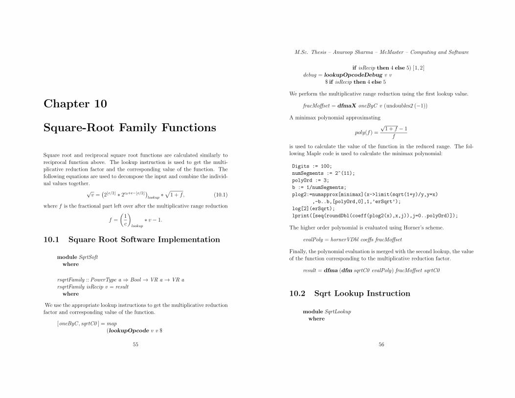
Chapter 10
Square-Root Family Functions
Square root and reciprocal square root functions are calculated similarly toreciprocal function above. The lookup instruction is used to get the multi-plicative reduction factor and the corresponding value of the function. Thefollowing equations are used to decompose the input and combine the individ-ual values together.
√v =
�2�e/2� ∗ 2c0+e−�e/2��
lookup∗�1 + f, (10.1)
where f is the fractional part left over after the multiplicative range reduction
f =
�1
c
�
lookup
∗ v − 1.
10.1 Square Root Software Implementation
module SqrtSoftwhere
rsqrtFamily :: PowerType a ⇒ Bool → VR a → VR arsqrtFamily isRecip v = resultwhere
We use the appropriate lookup instructions to get the multiplicative reductionfactor and corresponding value of the function.
[oneByC , sqrtC0 ] = map(lookupOpcode v v $
55
M.Sc. Thesis – Anuroop Sharma – McMaster – Computing and Software
if isRecip then 4 else 5) [1, 2]debug = lookupOpcodeDebug v v
$ if isRecip then 4 else 5
We perform the multiplicative range reduction using the first lookup value.
fracMoffset = dfmaX oneByC v (undoubles2 (−1))
A minimax polynomial approximating
poly(f) =
√1 + f − 1
f
is used to calculate the value of the function in the reduced range. The fol-lowing Maple code is used to calculate the minimax polynomial:
Digits := 100;
numSegments := 2^(11);
polyOrd := 3;
b := 1/numSegments;
plog2:=numapprox[minimax](x->limit(sqrt(1+y)/y,y=x)
,-b..b,[polyOrd,0],1,’erSqrt’);
log[2](erSqrt);
lprint([seq(roundDbl(coeff(plog2(x),x,j)),j=0..polyOrd)]);
The higher order polynomial is evaluated using Horner’s scheme.
evalPoly = hornerVDbl coeffs fracMoffset
Finally, the polynomial evaluation is merged with the second lookup, the valueof the function corresponding to the multiplicative reduction factor.
result = dfma (dfm sqrtC0 evalPoly) fracMoffset sqrtC0
10.2 Sqrt Lookup Instruction
module SqrtLookupwhere
56

M.Sc. Thesis – Anuroop Sharma – McMaster – Computing and Software
sqrtLookup :: Bool → Integer → (Integer , Integer)sqrtLookup isRecip v = (fstLookup, if isRecip
then rsqrtSndLookupelse sqrtSndLookup)
where
We have calculated the accurate table with 2n intervals, dividing the range[0, 1). For each interval we have calculated two values of sqrt , one with anadditional
√2 factor and the other without it, corresponding to whether the
input has an odd or even unbiased exponent.
n = 11
We boost the subnormal inputs into normal range by multiplying 252.
(sign, rest) = divMod v (2 ↑ 63)(exponent ,mantissa) = divMod rest (2 ↑ 52)( , leading0s) = countLeadingZeros 52 52 mantissa(adjustedExponent , adjustedMantissa) = case exponent of0 → (52− fromIntegral leading0s ,
mod (shiftL mantissa (leading0s + 1)) (2 ↑ 52))→ (exponent ,mantissa)
lookupKey is constructed using the leading n-bits of adjustedMantissa and thelast bit of adjustedExponent , which tells us whether the unbiased adjustedExponent
is even or odd.
lookupKey = bits 0 1 adjustedExponent ∗ (2 ↑ n)+ bits (52− n) 52 adjustedMantissa
[sqrtC , oneByC ] = (if isRecipthen rsqrtTableelse sqrtTable) !! fromIntegral lookupKey
We take the complement of the exponent to get −e+ 1+ 0x3ff.
exponentComplemented = xor adjustedExponent 0x7ffexponentFstLookup = exponentComplemented
+ bits 52 63 oneByCmantissaFstLookup = bits 1 52 oneByC
The multiplicative reduction factor is then constructed using the exponentcomplement and table value.
57
M.Sc. Thesis – Anuroop Sharma – McMaster – Computing and Software
fstLookup = case exponent of0 → sign ∗ (2 ↑ 63)
+ (exponentFstLookup + 52) ∗ (2 ↑ 51)+mantissaFstLookup
→ sign ∗ (2 ↑ 63)+ exponentFstLookup ∗ (2 ↑ 51)+mantissaFstLookup
Dividing the exponent by 2 is same as shifting the exponent right by 1 bit andletting the last bit drop off. We have taken care of the dropped off bit withthe lookup value.
adjustedExponentDiv2 = shiftR adjustedExponent 1
Since we have shifted the biased exponent, the bias also gets divided by 2.To fix the bias again, we add a constant 511 = div0x3ff2. In the case ofsubnormal inputs, an additional factor used for the boost needs to be included.
sqrtExpMultC| exponent ≡ 0 = adjustedExponentDiv2 ∗ (2 ↑ 52)
+ sqrtC − (511 ∗ 2 ↑ (52))− 26 ∗ 2 ↑ (52)| otherwise = adjustedExponentDiv2 ∗ (2 ↑ 52)
+ sqrtC − (511 ∗ 2 ↑ (52))
Finally, we override the second lookup value for special cases.
sqrtSndLookup| isNan v = 0x7ff8000000000000| div v (2 ↑ 63) ≡ 1 = 0x7ff8000000000000| div v (2 ↑ 52) ≡ 0x7ff = 0x7ff0000000000000| v ≡ 0 = 0| otherwise = sqrtExpMultC
Similar adjustments need to be done for reciprocal square root, wherethe complement of adjustedExponent is used to construct the value of thereciprocal square root function.
adjustedExpComplDiv2 = shiftR (xor 0x7ff adjustedExponent) 1rsqrtExpMultC
| exponent ≡ 0 = adjustedExpComplDiv2 ∗ (2 ↑ 52)
58

M.Sc. Thesis – Anuroop Sharma – McMaster – Computing and Software
+ sqrtC − (512 ∗ 2 ↑ (52)) + 26 ∗ 2 ↑ (52)| otherwise = adjustedExpComplDiv2 ∗ (2 ↑ 52)
+ sqrtC − (512 ∗ 2 ↑ (52))
Finally, we look for special inputs and override the second lookup with thecorrect function values.
rsqrtSndLookup| isNan v = 0x7ff8000000000000| div v (2 ↑ 63) ≡ 1 = 0x7ff8000000000000| div v (2 ↑ 52) ≡ 0x7ff = 0| v ≡ 0 = 0x7ff0000000000000| otherwise = rsqrtExpMultC
59
M.Sc. Thesis – Anuroop Sharma – McMaster – Computing and Software
60

Chapter 11
Exponential Family Functions
Exponential family functions are calculated using base 2. Inputs are scaledaccordingly. After scaling, we decompose the input into the integer part [x]and the fractional part, x − [x]. The fractional part is further decomposedusing accurate table values c and 2c, and we multiply the individual powers oftwo to get the result
2x = 2[x] ∗ 2x−[x]
= 2[x] ∗ 2c ∗ 2x−[x]−c
11.1 Exp Software Implementation
module ExpSoftwhere
expFamily :: PowerType a ⇒ MathOptions → Bool→ VR a → VR a
expFamily (MathOptions base exceptions) isM1Case v = resultwhere
We scale the input according the the base of the exponential to put the scaledinteger value into the high-order 11 bits into the mantissa. These bits in theexponent bit field will return 2[x].
61
M.Sc. Thesis – Anuroop Sharma – McMaster – Computing and Software
vScaledOffset = case base ofMO2 → dfa v offsetBumpMOe → dfma v invLog2 offsetBumpMOeX2 → dfma v invLog2X2 offsetBumpMO2m1 → dfnms v (undoubles2 1) offsetM1BumpMO2p1 → dfa v offsetM1BumpMOem1 → dfnms v invLog2 offsetM1BumpMOep1 → dfma v invLog2 offsetM1BumpMO10 → dfma v log10InvLog2 offset
Base MOeX2 represents the exponential function e2x, MO2m1 represents2−x−1 and MO2p1 represents 2x−1. These functions are used in the calcu-lation of hyperbolic functions and other functions not in the standard library.
Now we construct the reduction to (−0.5, 0.5) in two steps:
First, truncate the pseudo fixed-point version of the input to the mostsignificant fractional bits, using the odd instruction shufb.
v3Bytes = shufB1 vScaledOffset[0, 1, 2, shufb0x00 , shufb0x00 , shufb0x00 , shufb0x00 , shufb0x00, 8, 9, 10, shufb0x00 , shufb0x00 , shufb0x00 , shufb0x00 , shufb0x00 ]
Next subtract a modified fixed offset, to get a truncated version of theinput with 0.5 added. Now subtract this from the original input, to get thelow-order part of the fraction. This operation is exact, because the resultingexponent is not larger than the exponent of the input. To improve roundingduring range reduction, we use high and low-order double values,
frac = case base ofMO2 → dfs v (dfs v3Bytes offset)MOe → dfma v invLog2Low
(dfms v invLog2 (dfs v3Bytes offset))MOeX2 → dfma v invLog2LowX2
(dfms v invLog2X2 (dfs v3Bytes offset))MO2m1 → dfnma v (undoubles2 1)
(dfs v3Bytes offsetM1 )MO2p1 → dfs v (dfs v3Bytes offsetM1 )MOem1 → dfma v invLog2Low
(dfnma v invLog2 (dfs v3Bytes offsetM1 ))
62

M.Sc. Thesis – Anuroop Sharma – McMaster – Computing and Software
MOep1 → dfma v invLog2Low(dfms v invLog2 (dfs v3Bytes offsetM1 ))
MO10 → dfma v log10InvLog2 (dfs v3Bytes offset)
Then, table values are looked up using the vScaledOffset . The range reductionfactor c0 is in the same interval as frac. The corresponding value of functionexp2c0 , also includes the integer part = 2[x]+c.
[c0 , exp2c0 ] = map (lookupOpcode vScaledOffset vScaledOffset 1)[1, 2]
debug = lookupOpcodeDebug vScaledOffset vScaledOffset 1
Now, we reduce the range using first lookup value.
fracMOffset = dfmaX (undwrds2 0x3ff8000000000000) frac c0
2x−[x]−c is calculated using a minimax polynomial evaluated by Maple. Thefollowing Maple code calculates the minimax polynomial.Digits := 50;
pExp := numapprox[minimax](x -> 2^x, -1/256 .. 1/256
,[4, 0], 1, ’er’);
log[2](er);
lprint([seq(roundDbl(coeff(pExp, x, j)), j = 0 .. 4)]);In case of 2x − 1 (i.e., isM1Case ≡ True)
pExp := numapprox[minimax](x -> limit((2^y-1)/y,y = x)
,-1/256 .. 1/256, [4, 0], 1, ’er’);
log[2](er);
lprint([seq(roundDbl(coeff(pExp, x, j)), j = 0 .. 4)]);
evalPoly � = hornerVDbl coeffs fracMOffsetevalPoly = if isM1Case then dfm evalPoly � fracMOffset
else evalPoly �
The resultant polynomial evaluation is multiplied with the second lookup valueto generate the result.
result = if isM1Case then dfma evalPoly exp2c0$ dfs exp2c0 (undoubles2 1)else dfm evalPoly exp2c0
63
M.Sc. Thesis – Anuroop Sharma – McMaster – Computing and Software
11.2 Exp Lookup Instruction
module ExpLookupwhere
We put the integral part of input [x] into the desired bit position inthe mantissa by adding a power to 2, bumped by 0.5 for rounding. In oursoftware implementation of exponential family, we scaled the integer part ofthe input into the high-order 11 bits of the mantissa. An additional 1023 isalready added into integer part to account for biasing. This offset number isfed to the expLookup instruction which, based on table lookup, generates c0such that fracMc0 = x− [x]− c0 ∈ [−2−N , 2−N ], and 2[x]+c0.
expLookup :: Integer → (Integer , Integer)expLookup xOffset = (fstLookup, sndLookup)where
We have calculated the table of size 2n, such that it divides the range[−0.5, 0.5] into 2n segments.
(n, table) = (8, exp2Table)
The lookup key is the n-bits followed by the integer part of the input.
lookupKey = bits (40− n) 40 xOffset
We know the first table value, representing 2c0, belongs in the range [�
1/2,√2].
We only need to store the last bit of its exponent and mantissa bits. Similarmodifications could be made to c0, based on the smallest table value other than0, to reduce the size of table. This requires decomposing, storing, and com-posing in the hardware, which is not of particular interest as far as algorithmis concerned.
(lastBitExpC0 ,mantissaC0 , c0 ) = table !! fromIntegral lookupKey
expBits represents the value [x]+ 0x3ff.
expBits = bits 40 52 xOffset
64
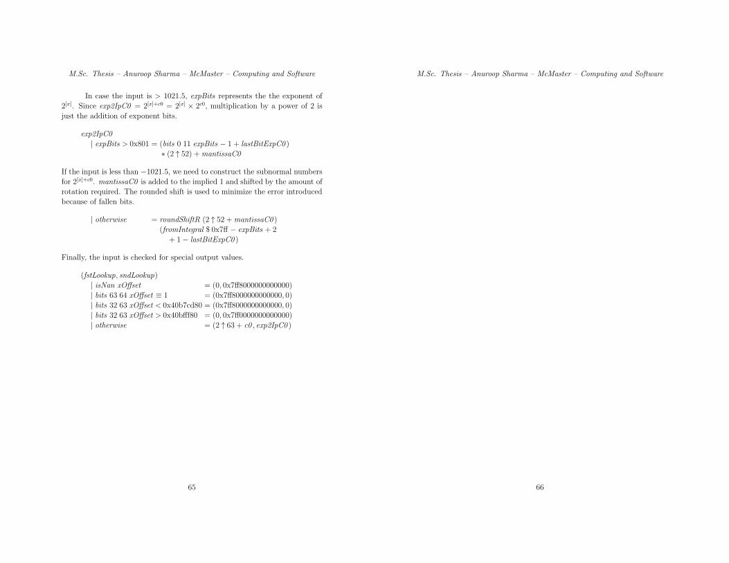
M.Sc. Thesis – Anuroop Sharma – McMaster – Computing and Software
In case the input is > 1021.5, expBits represents the the exponent of2[x]. Since exp2IpC0 = 2[x]+c0 = 2[x] × 2c0, multiplication by a power of 2 isjust the addition of exponent bits.
exp2IpC0| expBits > 0x801 = (bits 0 11 expBits − 1 + lastBitExpC0 )
∗ (2 ↑ 52) +mantissaC0
If the input is less than −1021.5, we need to construct the subnormal numbersfor 2[x]+c0. mantissaC0 is added to the implied 1 and shifted by the amount ofrotation required. The rounded shift is used to minimize the error introducedbecause of fallen bits.
| otherwise = roundShiftR (2 ↑ 52 +mantissaC0 )(fromIntegral $ 0x7ff − expBits + 2
+ 1− lastBitExpC0 )
Finally, the input is checked for special output values.
(fstLookup, sndLookup)| isNan xOffset = (0, 0x7ff8000000000000)| bits 63 64 xOffset ≡ 1 = (0x7ff8000000000000, 0)| bits 32 63 xOffset < 0x40b7cd80 = (0x7ff8000000000000, 0)| bits 32 63 xOffset > 0x40bfff80 = (0, 0x7ff0000000000000)| otherwise = (2 ↑ 63 + c0 , exp2IpC0 )
65
M.Sc. Thesis – Anuroop Sharma – McMaster – Computing and Software
66

Chapter 12
Trigonometric Family Functions
Trigonometric functions are calculated using the following standard identities:
sin(θ + φ) = sin(θ)cos(φ) + cos(θ)sin(φ)
cos(θ + φ) = cos(θ)cos(φ)− sin(θ)sin(φ)
The accurate table used for the calculation of trigonometric functions is dif-ferent from the tables of other functions. In this trigonometric table, we needto have three accurate values, the angle θ, and its sine and cosine values. Wehave calculated the table such that for each interval in the first half-quadrant,we found two integers such that the sum of their squares is as close to n2 aspossible. These integers are then converted to double floating point represen-tations and stored as sin(θ) and cos(θ). Then both high and low parts of θ arecalculated using high precision Maple. For the second half-quadrant, we justswitch between the sin and cos values; the high and low parts of correspondingangles are stored in the table.
12.1 Trigonometric Functions Software Imple-
mentation
module TrigSoftwhere
trigFamily :: PowerType a ⇒ VR a → (VR a,VR a,VR a)trigFamily v = (sin, cos , tan)where
67
M.Sc. Thesis – Anuroop Sharma – McMaster – Computing and Software
We mask off the sign bits from the input.
absV = andc v signBitDbl
Since we are using 27-segment intervals dividing the [0, pi/2) range, we multiplythe input by 29/(2π) to convert the angle in radians to an angle in fraction ofrotations, where each rotation is divided into 29 intervals. We add the offset= 252 to put the integral part of the segment number into the last 9-bits ofthe mantissa bits, where the bits from 9 leftward represent the number ofrotations.
vScaledOffset = dfma scaleHigh absV offset
The fractional part of the segment is dropped off in the calculation of vScaledOffset,hence subtracting the offset from vScaledOffset returns the integer part of thesegment.
intSegments = dfs vScaledOffset offset
Now we calculate the fractional part of the segment, by subtracting intSegmentsfrom the segment = 29v/(2π) itself. We use both high and low parts ofvOverPiHigh to get accuracy for the fractional part of the segment.
vOverPiHigh = dfm absV scaleHighvOverPiLow = dfms absV scaleLow vOverPiHighvOverPiReducedHigh = dfms absV scaleHigh intSegmentsvOverPiReduced = dfma absV scaleLow
vOverPiReducedHigh
Hardware lookup instructions return the high and low parts of the distanceof the angle with accurate values (its sine and cosine) from the start of thesegment. We use extended precision doubles for sine and cosine values in orderto handle the exceptional cases and very large inputs.
[thetaHigh, thetaLow , costheta, sintheta ]= map (lookupOpcode vScaledOffset vScaledOffset 6) [1, 2, 3, 4]
We subtract both parts of the theta from the fractional part of the segment.We use dfmaX in order to get 0 as fracMOffset for very large inputs.
fracMOffset = dfmaX oneX(dfmaX oneX vOverPiReducedHigh thetaHigh)(dfma absV scaleLow thetaLow)
68

M.Sc. Thesis – Anuroop Sharma – McMaster – Computing and Software
Since series expansions of both sine and cosine have interleaved powers of theinput, we calculate the minimax polynomial in terms of fracMOffset2.
fracMOffsetSquared = dfm fracMOffset fracMOffset
We calculate the minimax polynomials of the following functions to calculatethe sine and cosine in the reduced range.
polySin(x2) = minimax
�sin(x)− x
x3
�,
polyCos(x2) = minimax
�cos(x)− 1
x2
�,
where x is scaled to represent the fractional part of the segment. The Maplecode needed to generate these polynomials is:
Digits := 50;
numSegments := 128;
polyOrd := 2;
b := Pi/2 / numSegments;
pSin1:=numapprox[minimax](x->limit((sin(y)-y)/(y^3),y=sqrt(x))
,-1.5*b..1.5*b,[polyOrd,0],x->x^2,’erSin’);
pSin:=convert(evalf(eval(x + x^3 * pSin1(x^2)
,x=2*Pi*x/(2^9))),horner);
log[2](erSin);
lprint([seq(roundDbl(coeff(pSin,x,2*j+1)),j=0..polyOrd+1)]);
polyOrd := 3;
pCos1:=numapprox[minimax](x->limit((cos(y)-1)/(y^2),y=sqrt(x))
,-1.5*b..1.5*b,[polyOrd,0],x->x^2,’erCos’);
pCos:=convert(evalf(eval(1 + x^2 * pCos1(x^2)
,x=x*2*Pi/(2^9))),horner);
log[2](erCos);
lprint([roundDbl(1),seq(roundDbl(coeff(pCos,x,2*j+2))
,j=0..polyOrd)]);
We calculate the sine and cosine of the leftover value.
sinInSeg = dfm fracMOffset$ hornerVDbl sinCoeffs fracMOffsetSquared
cosInSeg = hornerVDbl cosCoeffs fracMOffsetSquared
69
M.Sc. Thesis – Anuroop Sharma – McMaster – Computing and Software
We use the mathematical identities given above to calculate the sine and cosineof the absolute value of the input.
absSin = dfmaX sintheta cosInSeg(dfmaX costheta sinInSeg zeroX )
cos = dfmaX costheta cosInSeg(dfm (dfmaX sintheta sinInSeg zeroX ) (undoubles2 $−1))
In the case of sine, we put back the sign.
sin = xor absSin (PowerType.and v signBitDbl)
We use the ratio of sine and cosine to calculate the tangent of the input.
tan = recipFamily True cos sin
12.2 Trig Lookup Instruction
module TrigLookupwhere
The lookup instruction returns the high and the low parts of the differenceof the angle with accurate sine and cosine values from the start of the seg-ment. The sine and cosine values are returned in extended precision doublerepresentation to handle the exceptional values.
trigLookup :: Integer → (Integer , Integer , Integer , Integer)trigLookup xOffset = (thetaHigh, thetaLow , cos , sin)where
The lookup key is constructed using the last 7 bits of the xOffset , representingthe segment in the quadrant. Bits 7 and 8 represent the quadrant in whichthe input lies.
lookupKey = bits 0 7 xOffsetquadrant = bits 7 9 xOffset
We retrieve the theta values from the table. In the case of large inputs, wereturn the value NaN as it would return zero as the result of range reduction.
70

M.Sc. Thesis – Anuroop Sharma – McMaster – Computing and Software
[thetaHigh, thetaLow ]| bits 52 63 xOffset�≡ 0x433 = [nan0X , nan0X ]
| otherwise = let [a, b ] = snd sincosTable!! fromIntegral lookupKey
in [2 ↑ 63 + a, 2 ↑ 63 + b ]
We construct the sine and cosine values from the table values, and we switchbetween the lookup key and its complement-based values based on whetherthe input lies in the odd or the even half-quadrant.
(costheta, sintheta) = case (quadrant , div lookupKey (2 ↑ 6)) of(0, 0) → fromKey lookupKey(0, 1) → switch $ fromKey (xor lookupKey (2 ↑ 7− 1))(1, 0) → let (a, b) = fromKey lookupKeyin (2 ↑ 63 + b, a)
(1, 1) → let (a, b) = fromKey (xor lookupKey (2 ↑ 7− 1))in (2 ↑ 63 + a, b)
(2, 0) → let (a, b) = fromKey lookupKeyin (2 ↑ 63 + a, 2 ↑ 63 + b)
(2, 1) → let (a, b) = fromKey (xor lookupKey (2 ↑ 7− 1))in (2 ↑ 63 + b, 2 ↑ 63 + a)
(3, 0) → let (a, b) = fromKey lookupKeyin (b, 2 ↑ 63 + a)
(3, 1) → let (a, b) = fromKey (xor lookupKey (2 ↑ 7− 1))in (a, 2 ↑ 63 + b)→ error "trigHWLookup.impossible happened"
Finally, we look for exceptional cases and return the corresponding values.
(cos , sin)| isNan xOffset = (nan0X , nan0X )
We detect very large inputs by comparing the exponent of the offsetted valuewith the exponent of the offset we added. If the input is very large, we return1/√2 for both sine and cosine values.
| bits 52 63 xOffset�≡ 0x433 = (nan2X , nan2X )
| otherwise = (costheta, sintheta)
71
M.Sc. Thesis – Anuroop Sharma – McMaster – Computing and Software
We construct the extended precision double values for the sine and cosinevalues, which we get from the table.
fromKey key = let ((cosE , cosM ), (sinE , sinM ))= fst sincosTable !! (fromIntegral key)
in (construct (cosE , cosM ), construct (sinE , sinM ))
construct (0, 0) = 0construct (0x3ff, 0) = 0x3ff8000000000000construct (e,m) = (0x400 + 0x3fe− e) ∗ (2 ↑ 51)
+m ∗ (2 ↑ (51− 32 + e + 1))
switch is a small helper function.
switch (a, b) = (b, a)
72

Chapter 13
Inverse Trigonometric FamilyFunctions
We implement all the inverse trigonometric functions using the atan2 function,with appropriate arguments. The core function, atan2, uses a hardware lookupinstruction to provide an angle for angle reduction and its tangent value. Thesearguments are used to reduce the inputs to smaller range near the x-axis, usingthe following rotation matrix.
�x�
y�
�=
1�1 + tan2(θ)
�1 tan(θ)
− tan(θ) 1
� �x
y
�(13.1)
Since we still need to divide the inputs after the rotation by −θ, the common
factor1�
1 + tan2(θ)is omitted in the computation.
13.1 Inverse Trigonometric Functions Software
Implementation
module InverseTrigSoftwhere
atan2Family :: PowerType a ⇒ VR a → VR a → VR aatan2Family y x = resultwhere
73
M.Sc. Thesis – Anuroop Sharma – McMaster – Computing and Software
The six hardware lookup instructions return the ordered inputs, the rotationangle, its tangent, and the adjustment we need to make based on the half-quadrant of the input co-ordinates.
[u, v , tanTheta, theta, adjust1 , adjust2 ]= map (lookupOpcode y x 7) [1 . . 6]
debug = lookupOpcodeDebug y x 7
We find the new co-ordinates after rotating by angle θ, to get co-ordinates inthe segment near 0.
uInSegment = dfma v tanTheta uvInSegment = dfnms u tanTheta v
We find the ratio of the new co-ordinates, representing the tangent of the anglein the segment.
tanInSegment = divDbl uInSegment vInSegment
The power series of the arctan function has the interleaved power in polyno-mial.
atan(x) = x− 1/3x3 + 1/5x5 +O(x6) (13.2)
We therefore find the minimax polynomial using Maple and the interleavedpowers.
poly(x2) = minimax
�atan(x)− x
x3
�(13.3)
The following maple code is used.Digits := 50;
polyOrd := 2;
numSegment := 2^(12);
b := 2/numSegment;
p := numapprox[minimax](x->limit((arctan(y)-y)/y^3,y=sqrt(x)),
-b..b,[polyOrd,0],1,’er’);log[2](er);
seq(roundDbl(coeff(p(x),x,i)),i=0..polyOrd);
tanInSegmentSquared = dfm tanInSegment tanInSegmentevalPoly = hornerVDbl ((undoubles2 1) : coeffs)
tanInSegmentSquared
The rotation angle is added to the evaluation of polynomial.
74
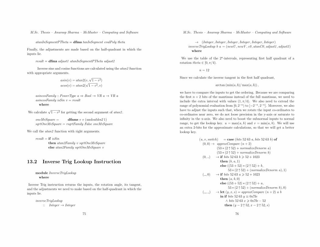
M.Sc. Thesis – Anuroop Sharma – McMaster – Computing and Software
atanInSegmentPTheta = dfma tanInSegment evalPoly theta
Finally, the adjustments are made based on the half-quadrant in which theinputs lie.
result = dfma adjust1 atanInSegmentPTheta adjust2
Inverse sine and cosine functions are calculated using the atan2 functionwith appropriate arguments.
asin(v) = atan2(v,√1− v2)
acos(v) = atan2(√1− v2, v)
asincosFamily :: PowerType a ⇒ Bool → VR a → VR aasincosFamily isSin v = resultwhere
We calculate√1− v2 for getting the second argument of atan2 .
oneMvSquare = dfnms v v (undoubles2 1)sqrtOneMvSquare = rsqrtFamily False oneMvSquare
We call the atan2 function with right arguments.
result = if isSinthen atan2Family v sqrtOneMvSquareelse atan2Family sqrtOneMvSquare v
13.2 Inverse Trig Lookup Instruction
module InverseTrigLookupwhere
Inverse Trig instruction returns the inputs, the rotation angle, its tangent,and the adjustments we need to make based on the half-quadrant in which theinputs lie.
inverseTrigLookup:: Integer → Integer
75
M.Sc. Thesis – Anuroop Sharma – McMaster – Computing and Software
→ (Integer , Integer , Integer , Integer , Integer , Integer)inverseTrigLookup b a = (newU , newV , c0 , atanC0 , adjust1 , adjust2 )where
We use the table of the 2n-intervals, representing first half quadrant of arotation theta ∈ [0, π/4).
n = 12
Since we calculate the inverse tangent in the first half quadrant,
arctan (min(a, b)/max(a, b)) ,
we have to compare the inputs to get the ordering. Because we are comparingthe first n + 2 bits of the mantissas instead of the full mantissas, we need toinclude the extra interval with values (1, π/4). We also need to extend therange of polynomial evaluation from [0, 2−n) to [−2−n, 2−n]. Moreover, we alsohave to adjust the inputs such that, when we rotate the input co-ordinates toco-ordinates near zero, we do not loose precision in the y-axis or saturate toinfinity in the x-axis. We also need to boost the subnormal inputs to normalrange, to get the lookup key. u = max(a, b) and v = min(a, b). We will usean extra 2-bits for the approximate calculations, so that we will get a betterlookup key.
(u, v , switch) = case (bits 52 63 a, bits 52 63 b) of(0, 0) → approxCompare (n + 2)
(53 ∗ (2 ↑ 52) + normalizeDenorm a)(53 ∗ (2 ↑ 52) + normalizeDenorm b)
(0, ) → if bits 52 63 b � 52 + 1023then (b, a, 1)else ((53 + 52) ∗ (2 ↑ 52) + b,
53 ∗ (2 ↑ 52) + (normalizeDenorm a), 1)( , 0) → if bits 52 63 a � 52 + 1023
then (a, b, 0)else ((53 + 52) ∗ (2 ↑ 52) + a,
53 ∗ (2 ↑ 52) + (normalizeDenorm b), 0)( , ) → let (y , x , s) = approxCompare (n + 2) a b
in if bits 52 63 y ≡ 0x7fe∧ bits 52 63 x � 0x7fe− 52then (y − 2 ↑ 52, x − 2 ↑ 52, s)
76

M.Sc. Thesis – Anuroop Sharma – McMaster – Computing and Software
else if bits 52 63 y � 52then (53 ∗ (2 ↑ 52) + y , 53 ∗ (2 ↑ 52) + x , s)else (y , x , s)
The maximum error introduced by these calculations is
u(1 + 2−(n+2)) >= v, (13.4)
where u = maxapprox(a, b) and v = minapprox(a, b).Now, we need to calculate the interval in which the input co-ordinates
lie. We can do so by approximating the v/u. This can be done by lookingup the estimate of the reciprocal of u from the reciprocal lookup table, thenapproximating their product based on the leading n-bits of their mantissas.
(eRecipEstU ,mRecipEstU ) = recipTable (n + 2) !!fromIntegral(bits (52− n − 2) 52 u)
(eApproxVByU ,mApproxVByU ) = approxMult (n + 2)mRecipEstU(bits (52− n − 2) 52 v)
The maximum error introduced by these calculations is
(u/v)(1 + 2n+2) >= (u/v)approx >= (u/v)(1− 2n+2). (13.5)
The combined error introduced in the lookup key calculation is therefore <
3∗2−(n+2). Since the accurate table values can be at either end of the interval,we have to double the range of the minimax polynomial.
Now we have to add the implied one to the approximate product andthen shift the resultant value to get the lookup key.
shift = bits 52 63 u − bits 52 63 v+ 1− eRecipEstU + 1− eApproxVByU + 2
lookupKey = roundShiftR (2 ↑ (n + 2) +mApproxVByU )(fromIntegral shift)
The values are retrieved from the table.
[c0 , atanC0 ] = arcTanTable !! fromIntegral lookupKey
According to the signs and ordering of the inputs, we need to adjust the result.
77
M.Sc. Thesis – Anuroop Sharma – McMaster – Computing and Software
signA = bits 63 64 asignB = bits 63 64 b(sign, rotation) = case (signA, signB , switch) of
(0, 0, 0) → (one, 0)(0, 0, 1) → (2 ↑ 63 + one, piBy2 )(1, 0, 1) → (one, piBy2 )(1, 0, 0) → (2 ↑ 63 + one, pi)(1, 1, 0) → (one, 2 ↑ 63 + pi)(1, 1, 1) → (2 ↑ 63 + one, 2 ↑ 63 + piBy2 )(0, 1, 1) → (one, 2 ↑ 63 + piBy2 )(0, 1, 0) → (2 ↑ 63 + one, 0)
Finally, we look for special inputs and overwrite the constants for uand v . These constants are returned because we do not want to generate NaNas a result of the calculation.
(newU , newV , adjust1 , adjust2 )| isZero a ∧ isZero b = (1, 1, 0, nan)| isInf a ∧ isInf b = (1, 1, 0, nan)| isNan a ∨ isNan b = (1, 1, 0, nan)| isZero a ∨ isZero b = (1, 1, 0, rotation)| isInf a ∨ isInf b = (1, 1, 0, rotation)| otherwise = (absU , absV , sign, rotation)
absU = bits 0 63 uabsV = bits 0 63 v
The following values recipExtU or approxUByV are useful for understand-ing the semantics of the instruction. These values are constructed for debugpurpose.
recipEstU = bits 63 64 u ∗ (2 ↑ 63) +(2046− bits 52 63 u+ eRecipEstU − 1) ∗ (2 ↑ 52)+mRecipEstU ∗ (2 ↑ (52− n))
approxVByU = xor (bits 63 64 u) (bits 63 64 v) ∗ (2 ↑ 63)+ (bits 52 63 v − bits 52 63 u+ 1023− 1 + eRecipEstU+ eApproxVByU − 1) ∗ (2 ↑ 52)+mApproxVByU ∗ (2 ↑ (52− n))
78

M.Sc. Thesis – Anuroop Sharma – McMaster – Computing and Software
This function boosts subnormal inputs to normal ranges by multiplying by252.
normalizeDenorm :: Integer → IntegernormalizeDenorm n = (bits 63 64 n) ∗ (2 ↑ 63)
+ (52− fromIntegral leading0s) ∗ (2 ↑ 52)+mod (shiftL mantissa (leading0s + 1)) (2 ↑ 52)
where( , leading0s) = countLeadingZeros 52 52 (bits 0 52 n)mantissa = mod n (2 ↑ 52)
This function compares the absolute values of the inputs based on the leadingn-bits of the mantissas.
approxCompare :: Int → Integer → Integer → (Integer , Integer , Int)approxCompare n a b = if bits (52− n) 63 a � bits (52− n) 63 b
then (a, b, 0)else (b, a, 1)
This is the approximate multiplication of the mantissas based on the first n-bits only. Since the result is ∈ [1, 4), we will return n-bits of the mantissa ofthe result and the exponent value ∈ {1, 2}.
approxMult :: Int → Integer → Integer → (Integer , Integer)approxMult n a b = case div result (2 ↑ n) of
1 → (1,mod result (2 ↑ n))→ (2,mod (roundShiftR result 1) (2 ↑ n))
wherem = (2 ↑ n + a) ∗ (2 ↑ n + b)result = div m (2 ↑ n)
79
M.Sc. Thesis – Anuroop Sharma – McMaster – Computing and Software
80

Chapter 14
Evaluation
We have implemented two types of simulations of these instructions. First, totest our accuracy claims, we implemented the new instructions in the Coconutinterpreter, adding them to the existing interpreter for Cell/B.E. SPU instruc-tions. The results were compared to results calculated by Maple with 500 sig-nificant digits of precision, and are reported in Table 14.1. As expected, theaccuracy results match the results for implementations using current Cell/B.E.SPU instructions. As the next step towards hardware implementation, we thenimplemented the instructions for logarithm using arrays of bits and logical op-erations, and verified that the results match the original implementations,which are written using integer and arbitrary-precision floating-point types inHaskell, and therefore both faster and easier to read.
14.1 Accuracy
We tested each of the functions by simulating execution using Coconut for atleast 20000 pseudo-random inputs over the full range and compared the resultsto computations carried out in Maple with 500 significant digits of precision.We found the maximum error of two ulps over all the functions. For detailssee table 14.1.
14.2 Performance
Since the dependency graphs (Figure 4.1) are nearly linear, the performance ofsoftware-pipelined loops will be proportional to the number of floating-point
81
M.Sc. Thesis – Anuroop Sharma – McMaster – Computing and Software
instructions. We report in Table 14.1 the expected throughput for vector mathfunctions which would result from adding these new instructions, assuming noother changes in the SPU execution model.
Table 14.1 reports the accuracy and performance statistics for the dif-ferent elementary functions. The size of the specific table is only reportedonce. No entry for the table size implies the table is being shared with someother instruction. The number of zero bits of excess precision in the accuratetable values is given, including the case log2 M = ∞ when all the table valuescan be chosen to be exact with the given table sizes. Other interpretation ofM is that some of the table values are exact, whereas other values are within1
Mof an ulp of an IEEE representable floating point number.
function cyclesdouble
cyclesdouble Speedup max error table poly log2 M
new SPU (%) (ulps) size(N) order
recip 3 11.3 376 0.500 2048 3 ∞div 3.5 14.9 425 1.333 recip 3sqrt 3 15.4 513 0.500 4096 3 18rsqrt 3 14.6 486 0.503 4096 3 ∞log2 2.5 14.6 584 0.500 4096 3 18
log21p 3.5 n/a n/a 1.106 log2 3log 3.5 13.8 394 1.184 log2 3
log1p 4.5 22.5 500 1.726 log2 3
exp2 4.5 13.0 288 1.791 256 4 18exp2m1 5.5 n/a n/a 1.29 exp2 4exp 5.0 14.4 288 1.55 exp2 4
expm1 5.5 19.5 354 1.80 exp2 4
atan2 7.5 23.4 311 0.955 4096 2 18atan 7.5 18.5 246 0.955 atan2 2+3asin 11 27.2 247 1.706 atan2 2+3+3acos 11 27.1 246 0.790 atan2 2+3+3
sin 11 16.6 150 1.474 128 3+3 52cos 10 15.3 153 1.025 sin 3+3tan 24.5 27.6 113 2.051 sin 3+3+3
Table 14.1: Accuracy and throughput (using Cell/B.E. SPU double precision)of standard functions with table sizes.
82

M.Sc. Thesis – Anuroop Sharma – McMaster – Computing and Software
Overall, the addition of hardware instructions to the SPU results in a3× improvement. Performance improvements on other architectures will vary,but would be significant.
The results (Table 14.1) show that the multiplicative reduction accuratetable method achieves nearly correctly rounded results for some functions likerecip, log2 and roots and high throughput for almost all the functions. On theCell/B.E. SPU, data-dependent branches are expensive, so we chose to imple-ment these functions in branch-free form, which costs several cycles to handleexceptional cases, but saves tens of cycles for mispredicted branches. For someinputs, typical implementations of the Newton-Raphson method produce in-correct results where producing correct results is considered too expensive.For example, in some implementations, recip is frequently allowed to saturateto ∞ for some subnormal inputs although the correcly rounded output wouldbe finite. This may be unacceptable for some applications, and it is a re-markable property of the library using the proposed instructions that no suchcompromises in the handling of rare cases were necessary.
83
M.Sc. Thesis – Anuroop Sharma – McMaster – Computing and Software
84

Chapter 15
Conclusion
We have demonstrated that when supported by a hardware lookup instructionand an extended-range fused multiply-add, we can achieve considerable per-formance and accuracy improvements for the elementary functions. In some ofthe functions, maximum errors as low as 0.500 ulps are achieved by combiningmultiplicative reduction using a fused multiply-add and accurate (or exact) ta-bles. Overall, using accurate tables for all the functions bounds the maximumerror to 2.051 ulps compared to more than 1000 ulps of error reported for theSPU MASS library. Our analysis has shown that new algorithms based onthe proposed hardware instructions would triple throughput on the Cell/B.E.SPU.
We showed by example that the new instructions are simple enough,certainly much simpler than floating point arithmetic, and would fit into thelatency and register-use requirements of conventional processors. We werealso able to handle all the exceptional cases internally in hardware, therebyeliminating the need for data dependent branches.
The work has been reported in a joint patent application [AES10] withIBM. To further reduce register pressure, we also proposed variants of thenew instructions with hidden internal state, and discuss the impact of such adecision on superscalar dispatch and required operating system support.
Although we have not explored it in this thesis, these methods areequally applicable to higher- and lower-precision floating point function eval-uation, although the table sizes and polynomial orders should be adjusted ifgreater performance is required processing 32-bit floats or better accuracy isrequired processing 128-bit (or higher) floats.
Finally, we acknowledge that although the proposed methods will pro-
85
M.Sc. Thesis – Anuroop Sharma – McMaster – Computing and Software
vide very high performance, some functions are not as accurate as we wouldlike, particularly, div , the exponentials and the trigonometric functions, butthere is some hope that taking rounding into account [BC07] when searchingfor both tables and polynomial values could reduce the maximum error.
86
Bibliography
[ACG+86] Ramesh C. Agarwal, James W. Cooley, Fred G. Gustavson,James B. Shearer, Gordon Slishman, and Bryant Tuckerman. Newscalar and vector elementary functions for the IBM System/370.IBM J. Res. Dev., 30(2):123–144, 1986.
[AES10] Christopher K. Anand, Robert Enenkel, and Anuroop Sharma.Hardware instructions to accelerate table-driven mathematicalfunction evaluation. United States Patent Application 12/788570,filed May 27, 2010.
[AK08] Christopher K. Anand and Wolfram Kahl. Synthesising and ver-ifying multi-core parallelism in categories of nested code graphs.In Michael Alexander and William Gardner, editors, Process Alge-bra for Parallel and Distributed Processing. Chapman & Hall/CRC,2008.
[AK09] Christopher K. Anand and Wolfram Kahl. An optimized Cell BEspecial function library generated by Coconut. IEEE Transactionson Computers, 2009.
[AS09] Christopher K. Anand and Anuroop Sharma. Unified tables forexponential and logarithm families. AdvOL Report 2009/2, Mc-Master University, 2009.
[AS10] Christopher K. Anand and Anuroop Sharma. Unified tables forexponential and logarithm families. ACM Transactions on Mathe-matical Software, 37(3), 2010.
[BC07] N. Brisebarre and S. Chevillard. Efficient polynomial L∞ approxi-mations. In Proceedings of the 18th IEEE Symposium on ComputerArithmetic, pages 169–176, Santa Monica, USA, 2007. IEEE Com-puter Society Press, Los Alamitos, CA.
[Bem63] R. W. Bemer. A note on range transformations for square root andlogarithm. Commun. ACM, 6(6):306–307, 1963.
87
M.Sc. Thesis – Anuroop Sharma – McMaster – Computing and Software
[BPBL06] Pieter Bellens, Josep M. Perez, Rosa M. Badia, and Jesus Labarta.CellSs: a programming model for the Cell BE architecture. In SC’06: Proceedings of the 2006 ACM/IEEE conference on Supercom-puting, page 86, New York, NY, USA, 2006. ACM.
[CKJM05] Manuel M. T. Chakravarty, Gabriele Keller, Simon Peyton Jones,and Simon Marlow. Associated types with class. In In POPL05: Proceedings of the 32nd ACM SIGPLAN-SIGACT symposiumon Principles of programming languages, pages 1–13. ACM Press,2005.
[Cor05] International Business Machines Corporation. PowerPC UserInstruction Set Architecture. IBM Systems and TechnologyGroup, http://www.ibm.com/developerworks/systems/library/es-archguide-v2.html, 2005.
[Cor08] International Business Machines Corporation. CellBroadband Engine Programming Handbook. IBMSystems and Technology Group, https://www-01.ibm.com/chips/techlib/techlib.nsf/productfamilies/PowerPC,2008.
[DTSS05] Son Dao Trong, Eric M. Schwarz, and Martin Schmookler. FPUimplementations with denormalized numbers. IEEE Trans. Com-put., 54(7):825–836, 2005.
[EL93] Milos D. Ercegovac and Tomas Lang. Multiplica-tion/division/square root module for massively parallel computers.Integr. VLSI J., 16(3):221–234, 1993.
[Gal86] Shmuel Gal. Computing elementary functions: A new approach forachieving high accuracy and good performance. In Proceedings ofthe Symposium on Accurate Scientific Computations, pages 1–16,London, UK, 1986. LNCS 235, Springer-Verlag.
[GB91] Shmuel Gal and Boris Bachelis. An accurate elementary mathe-matical library for the IEEE floating point standard. ACM Trans.Math. Softw., 17(1):26–45, 1991.
[IBM06] IBM Corp. Synergistic Processor Unit Instruction Set Architecture.IBM Systems and Technology Group, Hopewell Junction, NY, Oc-tober 2006.
[Jon95] Mark P. Jones. Functional programming with overloading andhigher-order polymorphism, 1995.
[KAC06] Wolfram Kahl, Christopher Kumar Anand, and Jacques Carette.Control-flow semantics for assembly-level data-flow graphs. In
88

M.Sc. Thesis – Anuroop Sharma – McMaster – Computing and Software
Wendy MacCaull, Michael Winter, and Ivo Duntsch, editors,RelMiCS 2005, volume 3929 of LNCS, pages 147–160. Springer,2006.
[KM97] Alan H. Karp and Peter Markstein. High-precision division andsquare root. ACM Trans. Math. Softw., 23(4):561–589, 1997.
[KM06] Peter Kornerup and Jean-Michel Muller. Choosing starting val-ues for certain Newton-Raphson iterations. Theor. Comput. Sci.,351(1):101–110, 2006.
[Mul05] Jean-Michel Muller. On the definition of ulp (x). Technical report,RR2005-09, LIP, ENS Lyon, France, 2005.
[PJ+03] Simon Peyton Jones et al. The Revised Haskell 98 Report. Cam-bridge University Press, 2003. Also on http://haskell.org/.
[Rus98] David M. Russinoff. A mechanically checked proof of IEEE com-pliance of the floating point multiplication, division and squareroot algorithms of the AMD K7 processor. LMS J. Comput. Math,1:148–200, 1998.
[SAG99] Martin S. Schmookler, Ramesh C. Agarwal, and Fred G. Gus-tavson. Series approximation methods for divide and square root inthe Power3(TM) processor. In ARITH ’99: Proceedings of the 14thIEEE Symposium on Computer Arithmetic, page 116, Washington,DC, USA, 1999. IEEE Computer Society.
[Sch95] Eric M. Schwarz. Rounding for quadratically converging algorithmsfor division and square root. In ASILOMAR ’95: Proceedings ofthe 29th Asilomar Conference on Signals, Systems and ComputersVolume II, page 600, Washington, DC, USA, 1995. IEEE ComputerSociety.
[Tak97] Naofumi Takagi. Generating a power of an operand by a tablelook-up and a multiplication. In ARITH ’97: Proceedings of the13th Symposium on Computer Arithmetic (ARITH ’97), page 126,Washington, DC, USA, 1997. IEEE Computer Society.
89