ELEMENTAL ABUNDANCES OF SOLAR SIBLING CANDIDATES

The Astrophysical Journal, 787:154 (17pp), 2014 June 1 doi:10.1088/0004-637X/787/2/154C© 2014. The American Astronomical Society. All rights reserved. Printed in the U.S.A.

ELEMENTAL ABUNDANCES OF SOLAR SIBLING CANDIDATES

I. Ramırez1, A. T. Bajkova2, V. V. Bobylev2,3, I. U. Roederer4, D. L. Lambert1, M. Endl1,W. D. Cochran1, P. J. MacQueen1, and R. A. Wittenmyer5,6

1 McDonald Observatory and Department of Astronomy, University of Texas at Austin, 2515 Speedway, Stop C1400, Austin, Texas 78712-1205, USA2 Central (Pulkovo) Astronomical Observatory of RAS, 65/1, Pulkovskoye Chaussee, St. Petersburg 196140, Russia3 Sobolev Astronomical Institute, St. Petersburg State University, Bibliotechnaya pl. 2, St. Petersburg 198504, Russia

4 Department of Astronomy, University of Michigan, 500 Church Street, Ann Arbor, MI 48109, USA5 School of Physics, UNSW Australia, Sydney 2052, Australia

6 Australian Centre for Astrobiology, University of New South Wales, UNSW Kensington Campus, Sydney 2052, AustraliaReceived 2014 February 14; accepted 2014 April 7; published 2014 May 14

ABSTRACT

Dynamical information along with survey data on metallicity and in some cases age have been used recently bysome authors to search for candidates of stars that were born in the cluster where the Sun formed. We have acquiredhigh-resolution, high signal-to-noise ratio spectra for 30 of these objects to determine, using detailed elementalabundance analysis, if they could be true solar siblings. Only two of the candidates are found to have solar chemicalcomposition. Updated modeling of the stars’ past orbits in a realistic Galactic potential reveals that one of them,HD 162826, satisfies both chemical and dynamical conditions for being a sibling of the Sun. Measurements ofrare-element abundances for this star further confirm its solar composition, with the only possible exception ofSm. Analysis of long-term high-precision radial velocity data rules out the presence of hot Jupiters and confirmsthat this star is not in a binary system. We find that chemical tagging does not necessarily benefit from studying asmany elements as possible but instead from identifying and carefully measuring the abundances of those elementsthat show large star-to-star scatter at a given metallicity. Future searches employing data products from ongoingmassive astrometric and spectroscopic surveys can be optimized by acknowledging this fact.

Key words: stars: abundances – stars: fundamental parameters – stars: general – stars: individual (HD 162826) –stars: kinematics and dynamics

Online-only material: color figures, machine-readable tables

1. INTRODUCTION

Infrared surveys and observations of young stars made overthe past two decades suggest that most stars (80%–90%) areborn in rich clusters of more than 100 members inside giantmolecular clouds (Lada & Lada 2003; Porras et al. 2003; Evanset al. 2009). Although it has been pointed out that, depending onthe definition of cluster, the fraction of stars born in them couldbe as low as 45% (Bressert et al. 2010), there is convincingevidence that the Sun was born in a moderately large stellarsystem.

Daughter products of short-lived (<10 Myr) radioactivespecies have been found in meteorites, suggesting that theradioactive isotopes themselves were present in the early solarsystem (e.g., Goswami & Vanhala 2000; Tachibana & Huss2003). A nearby supernova explosion could have injected theseisotopes into the solar nebula (e.g., Looney et al. 2006), anevent that has a high probability in a dense stellar environment(e.g., Williams & Gaidos 2007). Additional evidence that theSun was born in such an environment is provided by thedynamics of outer solar system objects like Sedna (Brown et al.2004), which has large eccentricity (e ∼ 0.8) and perihelion(∼75 AU). Numerical simulations show that these extremeorbital properties can arise from close encounters with otherstars (e.g., Morbidelli & Levison 2004).

In his review of “The Birth Environment of the Solar System,”Adams (2010) concludes that the Sun was born in a cluster of103–104 stars. The probability of close stellar encounters andnearby supernova pollution is high in a bound cluster with morethan ∼103 members. On the other hand, the upper limit of ∼104

is set by the conditions that the solar system planets’ orbits mustbe stable and that the early UV radiation fields were not strong

enough to evaporate the solar nebula. Pfalzner (2013) arguesthat the Sun most likely formed in an environment resemblingan OB association (as opposed to a starburst cluster), where stardensities are not sufficient for the destruction of protoplanetarydisks due to stellar encounters.

The mean lifetime of open clusters in the Galactic disk isestimated to be about 100 Myr (Janes et al. 1988). Consideringthe solar system age of 4.57 Gyr (Bouvier & Wadhwa 2010), itis not surprising that the solar cluster is now fully dissipated andits members scattered throughout the Galaxy. The hypothesisthat the Sun was born in the solar-age, solar-metallicity opencluster M67 (Johnson & Sandage 1955; Demarque et al. 1992;Randich et al. 2006), which hosts some of the most Sun-likestars known (Pasquini et al. 2008; Onehag et al. 2011, 2014),has been refuted by Pichardo et al. (2012) using dynamicalarguments. These authors even conclude that the Sun and M67could not have been born in the same giant molecular cloud.

Stars that were born together with the Sun are referred to as“solar siblings.” They should not be confused with “solar twins,”which are stars with high-resolution, high signal-to-noise ratio(S/N) spectra nearly indistinguishable from the solar spectrum,regardless of their origin (Porto de Mello & da Silva 1997;Melendez & Ramırez 2007; Ramırez et al. 2011; Monroe et al.2013). By definition, the siblings of the Sun must have solar ageand solar chemical composition because they formed essentiallyat the same time from the same gas cloud. They do not need tobe “Sun-like” with respect to their fundamental parameters suchas effective temperature, mass, luminosity, or surface gravity.

In principle, the siblings of the Sun could be found by mea-suring accurately and with high precision the ages and detailedchemical compositions of large samples of stars, an approachthat is obviously impractical. Fortunately, analytical models of

1

http://dx.doi.org/10.1088/0004-637X/787/2/154

The Astrophysical Journal, 787:154 (17pp), 2014 June 1 Ramırez et al.

the Galactic potential can be used to predict their present-daydynamical properties. Alternatively, the same models can beemployed to determine in retrospect if a given star could havepossibly originated within the solar cluster. Thus, by applyingdynamical constraints, manageable samples of solar sibling can-didates can be constructed to be later examined carefully usingmore expensive methods such as high-resolution spectroscopy.

Thus, the Galactic mass distribution model by Miyamoto& Nagai (1975), as given in Paczynski (1990), was used byPortegies Zwart (2009) to reverse the orbit of the Sun andcalculate its birthplace in the Galaxy. The orbits of simulatedsolar clusters with 2,048 members were then computed todetermine the fraction of solar siblings to be found today inthe solar neighborhood. Portegies Zwart concludes that 10–60of them should be found within 100 pc from the Sun. Thissomewhat optimistic view was challenged by Mishurov &Acharova (2011), who employed the Galactic potential by Allen& Santillan (1991) and perturbed it with both quasi-stationary(Lin et al. 1969) and transient (Sellwood & Binney 2002) spiraldensity waves to show that the orbits of solar siblings stronglydeviate from being nearly circular. Mishurov & Acharova findthat only a few solar siblings may be found within 100 pcfrom the Sun if the solar cluster had ∼103 members. Thesituation might be worse if scattering by molecular clouds orclose stellar encounters were to be taken into consideration, but“less hopeless” if the solar cluster contained ∼104 stars instead.

Following the modeling by Portegies Zwart (2009), Brownet al. (2010) pointed out that one could use the regions of phase-space occupied by the simulated stars to narrow down the searchfor the siblings of the Sun. Their calculations suggest that thesestars should have proper motions lower than 6.5 mas yr−1 andparallaxes larger than 10 mas. Then, by employing data fromthe Hipparcos catalog (Perryman et al. 1997), in its revisedversion (van Leeuwen 2007), they were able to find the 87stars satisfying these conditions, after imposing an additionalconstraint of 10% for the precision of the parallaxes. Theirlist of candidates was further narrowed down by excludingstars with (B − V ) < 0.5, which are bluer than the solar-age isochrone turnoff. Finally, they employed the stellar agesgiven in the Geneva–Copenhagen Survey (GCS; Nordstromet al. 2004; Holmberg et al. 2007, 2009) to find the six starswith solar age within the errors. Based on the radial velocities(RVs) and metallicities given in the GCS, Brown et al. concludethat only one star (HD 28676) may be a true solar sibling. Fiveother candidates with (B−V ) > 1.0 were not found in the GCS.

A procedure similar to the one described above was adoptedby Batista & Fernandes (2012), but employing in addition tothe GCS other metallicity data sets (namely, Cayrel de Strobelet al. 2001, Feltzing et al. 2001, and Valenti & Fischer 2005). Byselecting stars with −0.1 < [Fe/H] < +0.1 and using the sameproper motion and parallax constraints described above, theycreated a list of 21 candidates for siblings of the Sun. Then, theyused the previously published stellar atmospheric parametersand the PARAM code by da Silva et al. (2006)7 to estimateisochrone ages for those stars and thus find the nine objects withsolar age within the errors. Further examination of the availabledata led them to conclude that the stars HD 28676 (alreadysuggested by Brown et al. 2010), HD 83423, and HD 175740(the first giant proposed as candidate) could all well be true solarsiblings.

The problem of searching for solar siblings in the solar neigh-borhood using existing survey data was tackled also by Bobylev

7 http://stev.oapd.inaf.it/cgi-bin/param

et al. (2011). They suggested a different method for findingthem. First, targets were searched using the stars’ Galactic spacevelocities U,V,W (their data set is described in Bobylev et al.2010) by excluding those whose total speeds relative to the solarone are significantly different (

√U 2 + V 2 + W 2 > 8 km s−1).

Then, the orbits of the remaining objects (162 FGK stars withparallax errors lower than 15%) were simulated backward intime using the Allen & Santillan (1991) Galactic potential per-turbed by spiral density waves (as suggested by Mishurov &Acharova 2011) to determine parameters of encounter with thesolar orbit such as relative distance and velocity difference overa period of time comparable to the Sun’s age. Finally, theseparameters were examined to calculate the probability that anyof these objects was born together with the Sun. Their calcu-lations rule out HD 28676 and HD 192324, both solar siblingcandidates according to Brown et al. (2010). On the other hand,Bobylev et al. list as their best candidates the stars HD 83423and HD 162826. Note that the former is also a good candidateaccording to Batista & Fernandes (2012). Furthermore, the cal-culated dynamic properties of this star seem to be very robustunder different model parameters.

In this work, we perform chemical analysis using newly ac-quired high-resolution, high S/N spectra to establish if any ofthe stars discussed above can be considered a true solar sibling.Finding these objects could shed light onto our origins. For ex-ample, knowledge of the spatial distribution of solar siblings canhelp determine the Sun’s birthplace and understand the impor-tance of radial mixing in shaping the properties of disk galaxies(Bland-Hawthorn et al. 2010). It will also enable us to better con-strain the physical characteristics of the environment in whichour star was born (Adams 2010). Furthermore, theoretical cal-culations show that large impacts of rocks into planets producefragments where primitive life can survive as they travel to otherplanets or even other nearby planetary systems, a mechanismknown as “lithopanspermia” (Adams & Spergel 2005; Valtonenet al. 2009; Belbruno et al. 2012). For example, Worth et al.(2013) estimate that about 5% of impact remains from Earthhave escaped the solar system. A similar value is obtained forthe case of Mars. Valtonen et al. (2012) point out that the possi-bility of contamination of solar siblings by “spores of life” fromour planet should make the siblings of the Sun prime targets inthe search for extraterrestrial life.

As we enter the era of massive, far-reaching astrometric/photometric surveys led by Gaia (Lindegren et al. 2012) as wellas comparably large high-resolution spectroscopic surveys suchas Gaia-ESO (Gilmore et al. 2012) and GALactic Archaeologywith HERMES (GALAH; Zucker et al. 2012), a thoroughinvestigation of the available data, albeit relatively small in thecontext of solar sibling research, must be made to guide themore statistically significant search strategies of the near future.

2. SAMPLE AND SPECTROSCOPIC ANALYSIS

2.1. The Solar Sibling Candidates

Our target list consists of all interesting objects discussedin the previous exploratory searches by Brown et al. (2010,hereafter Br10), Bobylev et al. (2011, hereafter Bo11), andBatista & Fernandes (2012, hereafter Ba12).8 In addition tothe six candidates listed in Table 1 of Br10, i.e., those they

8 Very recently, Batista et al. (2014) employed the detailed elementalabundance analysis of one of the largest exoplanet host star samples to findanother solar sibling candidate: HD 186302. We did not include this star in ourwork.

2

http://stev.oapd.inaf.it/cgi-bin/param


Table 1Solar Sibling Candidates

HD V SpT a d b σ (d)b Observedc RV σ (RV) Referenced

(mag) (pc) (pc) (km s−1) (km s−1)

7735 7.91 F5 85.7 8.8 McD – 2012 Dec 28.6 0.2 Ba1226690 5.29 F2V 36.3 0.8 McD – 2012 Dec 16.0 0.1 Ba1228676 7.09 F5 38.7 0.9 McD – 2012 Dec 6.4 0.1 Br10+Ba1235317nw 6.14 F7V 55.7 2.4 McD – 2012 Dec 15.0 0.1 Ba1244821 7.37 K0V 29.3 0.5 McD – 2012 Dec 14.6 0.1 Br10+Ba1246100 9.38 G8V 55.5 2.6 LCO – 2013 Apr 21.0 0.3 Ba1246301 7.28 F5V 107.6 6.6 McD – 2012 Dec −4.7 0.1 Ba1252242 7.41 F2V 68.2 2.7 McD – 2012 Dec 31.3 0.9 Ba1283423 8.78 F8V 72.1 4.9 McD – 2012 Dec −4.1 0.1 Bo11+Ba1291320 8.43 G1V 90.5 6.9 McD – 2012 Dec 16.6 0.2 Br1095915 7.25 F6V 66.6 2.1 LCO – 2013 Apr 19.2 0.3 Ba12100382 5.89 K1III 94.0 3.0 LCO – 2013 Apr −8.5 0.3 Br10101197 8.74 G5 83.0 6.8 McD – 2012 Dec 11.9 0.4 Ba12102928 5.63 K0III 91.4 4.2 McD – 2012 Dec 14.4 0.1 Br10105000 7.91 F2 71.1 3.0 McD – 2012 Dec −13.8 0.1 Ba12105678 6.34 F6IV 74.0 1.7 McD – 2013 Mar −19.5 0.3 Ba12147443 8.74 G5 92.0 8.4 McD – 2013 Mar 8.1 0.2 Br10148317 6.70 G0III 79.6 3.5 McD – 2013 Mar −37.9 0.1 Ba12154747 8.73 G8IV 97.8 8.9 LCO – 2013 Apr −14.9 0.3 Ba12162826 6.56 F8V 33.6 0.4 McD – 2012 Dec 1.7 0.1 Bo11168442 9.66 K7V 19.6 0.6 McD – 2012 Dec −14.3 0.2 Br10168769 9.37 K0V 50.2 3.7 LCO – 2013 Apr 26.3 0.2 Br10175740 5.44 G8III 82.0 1.7 McD – 2012 Dec −9.8 0.1 Br10+Ba12183140 9.30 G8V 71.8 6.6 LCO – 2013 Apr −30.0 0.1 Ba12192324 7.66 F8 67.1 4.8 LCO – 2013 Apr −3.8 0.2 Br10196676 6.45 K0 74.4 2.8 McD – 2012 Dec −0.5 0.2 Br10199881 7.49 F5 72.2 3.6 McD – 2012 Dec −16.7 0.1 Ba12199951 4.67 G6III 70.2 1.3 McD – 2012 Dec 18.2 0.2 Ba12207164 7.54 F2 76.1 3.8 McD – 2012 Dec −6.7 0.1 Ba12219828 8.05 G0IV 72.3 3.9 McD – 2012 Dec −24.3 0.1 Ba12

Notes.a Spectral type from SIMBAD.b Distance derived from Hipparcos parallax.c McD: Tull spectrograph on the 2.7 m Harlan J. Smith Telescope at McDonald Observatory. LCO: MIKE spectrograph on the 6.5 mMagellan/Clay Telescope at Las Campanas Observatory.d Br10: Brown et al. 2010; Bo11: Bobylev et al. 2011; Ba12: Batista & Fernandes 2012.

found in the GCS catalog, we also observed the five stars with(B − V ) > 1.0 that satisfied all other criteria for solar siblingcandidates in that work. The two stars discussed in detail inBo11 were also included. Finally, all 21 stars in the extendedlist by Ba12 (see their Table A) were observed. Note that Ba12’slist includes one object from Bo11 and three from Br11. Thus,a total of 30 targets were observed for this work (Table 1).

2.2. Spectroscopic Observations

We used the Tull coude spectrograph on the 2.7 m Har-lan J. Smith Telescope at McDonald Observatory (Tull et al.1995) to observe most of our targets (23). All but three ofthem were observed in 2012 December; the others were ob-served in 2013 March. The rest of our targets (seven) havetoo-low declinations to be observed from McDonald Observa-tory. Instead, they were observed using the Magellan InamoriKyocera Echelle (MIKE) spectrograph on the 6.5 m Telescopeat Las Campanas Observatory (Bernstein et al. 2003) in 2013April. Slit sizes were chosen so that the spectral resolution ofthe data is about 60,000 in the visible part of the spectrum.We targeted a S/N per pixel of at least 200 at 6000 Å. Onlyone of our targets (HD 46100) has a significantly lower S/Nspectrum.

The Tull/McDonald spectra were reduced in the stan-dard manner using the echelle package in IRAF9 while theMIKE/Magellan data were reduced using the CarnegiePythonpipeline.10 After correcting for the Earth’s motion using the rv-correct task in IRAF, the RVs of our target stars were measuredby cross-correlation with the spectra of stars in our sample withknown stable RVs. For the McDonald data we used as RV stan-dards the stars HD 196676 (RV = −0.5 km s−1) and HD 219828(RV = −24.1 km s−1). Their RVs are from Chubak et al. (2012).Three of the stars observed from Las Campanas have RVs in theGCS catalog (HD 46100, RV = 21.0 ± 0.2 km s−1; HD 183140,RV = −29.3 ± 0.1 km s−1; and HD 192324, RV = −4.4 ± 0.2).In all cases, regardless of which stars are used as standards,the resulting RV values are robust. They are given in Table 1.Formal, internal errors on our RV values are typically around0.2 km s−1. These errors are due to the order-to-order cross-correlation velocity scatter and the uncertainties in the veloci-ties of the standard stars. Systematic uncertainties will increasethese errors by at least 0.5 km s−1.

9 IRAF is distributed by the National Optical Astronomy Observatory, whichis operated by the Association of Universities for Research in Astronomy(AURA) under cooperative agreement with the National Science Foundation.10 http://code.obs.carnegiescience.edu/mike

3

http://code.obs.carnegiescience.edu/mike


0.60.70.80.91.0

SunFeI

FeI

BaII

CrIFeI

FeI

0.60.70.80.91.0

HD26690

0.60.70.80.91.0

HD46301

0.60.70.80.91.0

HD52242

0.60.70.80.91.0

HD105000

0.60.70.80.91.0

HD105678

5852 5853 5854 5855 5856Wavelength (Å)

0.60.70.80.91.0

HD147443

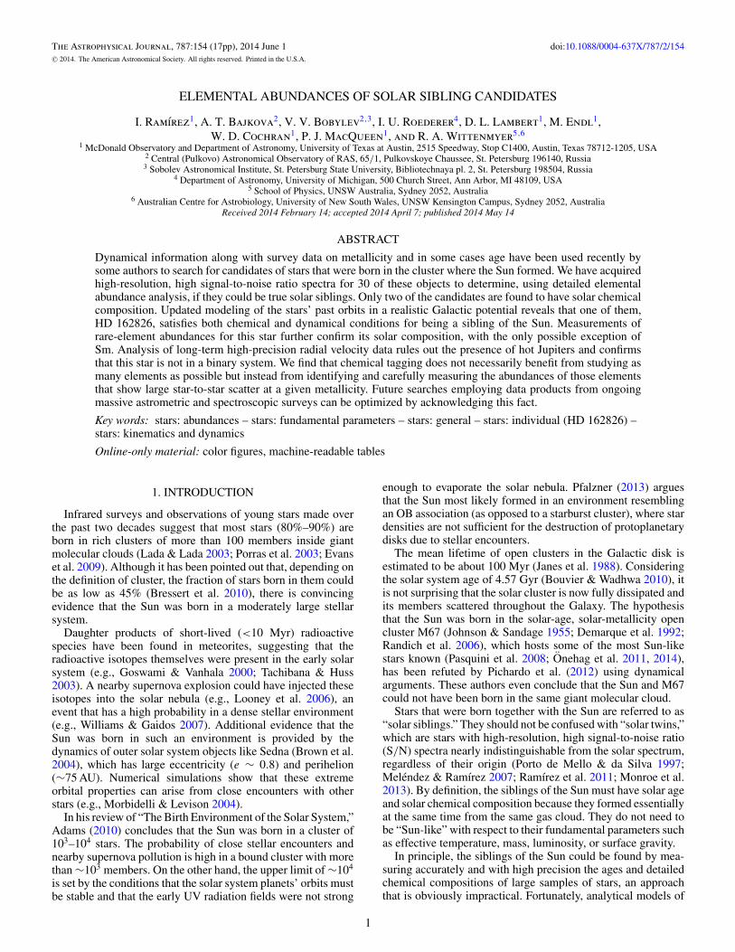
Figure 1. Spectra of high-V sin i stars. Our solar (Vesta) spectrum is shown inthe top panel for comparison.

(A color version of this figure is available in the online journal.)

2.3. Moderately Fast Rotators and Double-linedSpectroscopic Binaries

The methods that we employ to derive atmospheric param-eters and to measure elemental abundances (see Sections 2.4and 2.6) are not suited for stars with high projected rotationalvelocity (V sin i) or double-lined spectroscopic binaries (SB2s).The spectral lines in the former are either severely blended orthey cannot be identified due to the extreme rotational broad-ening. The SB2s, on the other hand, require special treatmentbecause even in cases where both sets of spectral lines can beidentified and measured independently, the blended continuumflux must be first estimated from previous knowledge of the twostars, making the problem somewhat degenerate and the resultsnot as accurate as those that can be achieved for single spec-tra stars. More importantly, in most cases these stars have beenselected because their photometry suggests a solar metallicity.Photometric calibrations of metallicity should only be appliedto single stars.

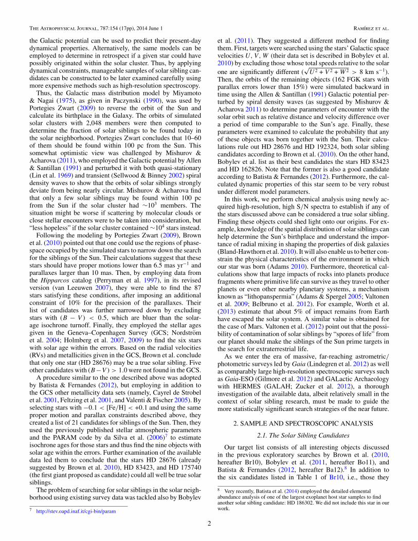
Figures 1 and 2 show the small spectral region of ourspectroscopic data containing the 5853.7 Å Ba ii line forour target stars with very high V sin i and targets that areSB2s, respectively. For reference, our solar (Vesta) spectrumis shown in the top panel of these figures. The SB2 nature ofHD 101197 and especially HD 183140 is obvious. The spectraof HD 7735 and HD 35317 show excess absorption on the bluewings of all spectral lines. The latter in fact has a very highV sin i companion, which was not analyzed in this work (hencethe “nw” flag, which stands for northwest component). StarHD 168442 has a spectrum that is irreproducible with single-

0.60.70.80.91.0

SunFeI

FeI

BaII

CrIFeI

FeI

0.60.70.80.91.0

HD7735

0.60.70.80.91.0

HD35317nw

0.60.70.80.91.0

HD101197

0.60.70.80.91.0

HD168442

0.60.70.80.91.0

HD183140

5852 5853 5854 5855 5856Wavelength (Å)

0.60.70.80.91.0

HD192324

Figure 2. Spectra of double-lined spectroscopic binary (SB2) stars. Our solar(Vesta) spectrum is shown in the top panel for comparison.


star models. It appears to be a blend of a Sun-like star and anM-type dwarf. Star HD 192324 has a very nearby companionwhich appears to have contaminated our spectrum. Even thoughthis star can be analyzed and stellar parameters were determinedas described in Section 2.4, a very clear trend of iron abundancewith wavelength persists, suggesting that the line strengths havebeen affected by the contribution to the continuum of the nearbyand probably very cool companion.

All moderately fast rotators and SB2s were excluded fromfurther analysis. Therefore, hereafter our sample is reduced to18 stars.

2.4. Stellar Parameter Determination

We employed the standard technique of excitation/ionizationbalance of iron lines to determine the stars’ atmospheric pa-rameters Teff (effective temperature), log g (surface gravity),[Fe/H] (iron abundance), and vt (microturbulence). The detailsof this method have been described multiple times, for examplein Ramırez et al. (2009, 2011, 2013). Basically, the equivalentwidths of a large number of nonblended, unsaturated Fe i andFe ii lines are measured using Gaussian line profile fits. In ourcase, this was done using IRAF’s splot task. Then, a standardcurve-of-growth approach is employed to determine the ironabundance from each line for a given set of guess stellar param-eters.

We used the spectrum synthesis code MOOG (Sneden1973)11 and Model Atmospheres in Radiative and Convective

11 http://www.as.utexas.edu/∼chris/moog.html

4

http://www.as.utexas.edu/~chris/moog.html


Table 2Iron Line List

Wavelength Speciesa EP log gf

(Å) (eV)

4779.44 26.0 3.42 −2.164788.76 26.0 3.24 −1.734799.41 26.0 3.64 −2.134808.15 26.0 3.25 −2.694961.91 26.0 3.63 −2.195044.211 26.0 2.851 −2.0585054.64 26.0 3.64 −1.985187.91 26.0 4.14 −1.265197.94 26.0 4.3 −1.545198.71 26.0 2.22 −2.14...

.

.

....

.

.

.

Note. a The number to the left of the decimal pointindicates the atomic number. The number to the rightof the decimal point indicates the ionization state,where “0” is neutral and “1” is singly ionized.

(This table is available in its entirety in a machine-readable form in the online journal. A portion isshown here for guidance regarding its form andcontent.)

Scheme (MARCS) model atmospheres with standard chemicalcomposition (Gustafsson et al. 2008)12 for our iron abundancecalculations. The initial-guess stellar parameters were iterativelymodified until the correlations between iron abundance and ex-citation potential (EP) and reduced equivalent width of the linedisappear while simultaneously enforcing agreement betweenthe mean iron abundances inferred from Fe i and Fe ii linesseparately. For these calculations, we employed relative ironabundances, i.e., the iron abundances were measured differen-tially with respect to the Sun, on a line-by-line basis, and usingthe reflected sunlight spectrum of the asteroid Vesta, taken fromMcDonald Observatory in 2012 December.

Formal errors for our spectroscopically derived stellar pa-rameters were calculated as described in Appendix B of Bensbyet al. (2014) and in Section 3.2 of Epstein et al. (2010). These

12 Available online at http://marcs.astro.uu.se.

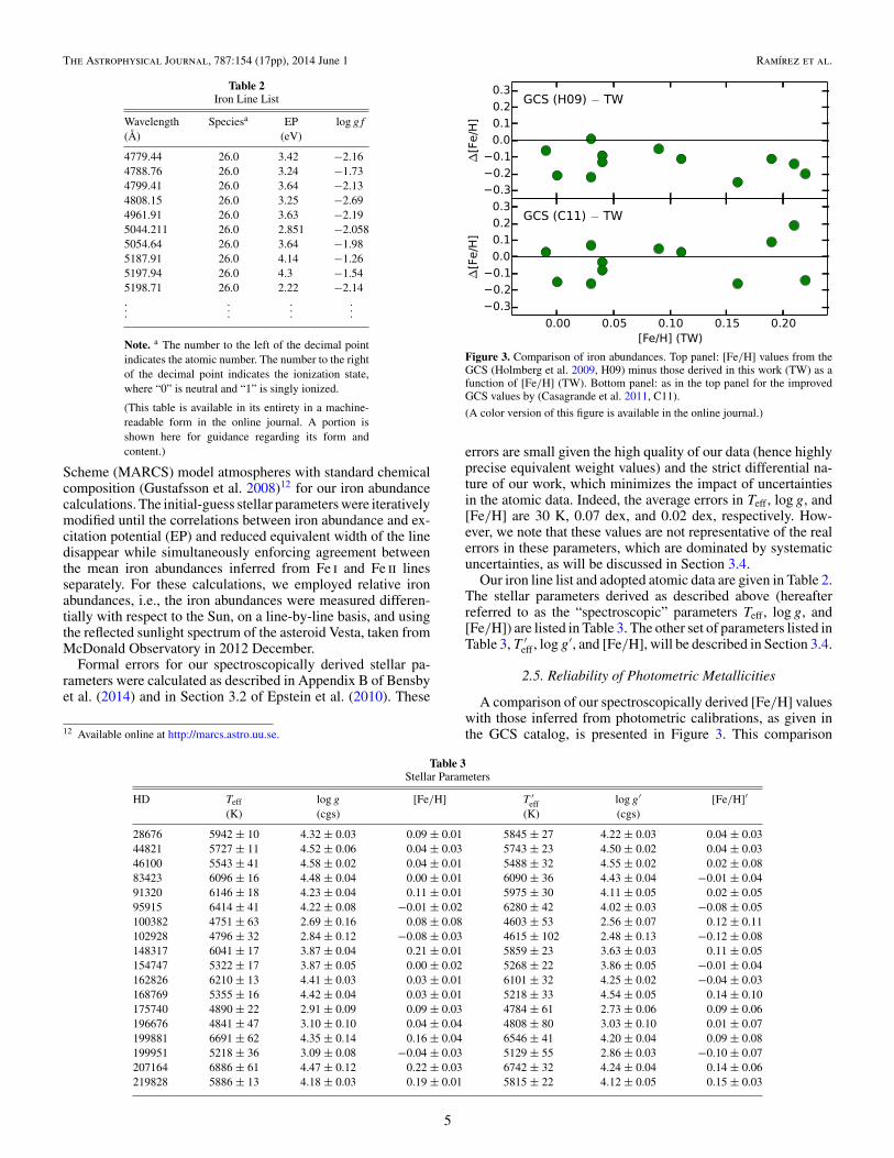
Figure 3. Comparison of iron abundances. Top panel: [Fe/H] values from theGCS (Holmberg et al. 2009, H09) minus those derived in this work (TW) as afunction of [Fe/H] (TW). Bottom panel: as in the top panel for the improvedGCS values by (Casagrande et al. 2011, C11).


errors are small given the high quality of our data (hence highlyprecise equivalent weight values) and the strict differential na-ture of our work, which minimizes the impact of uncertaintiesin the atomic data. Indeed, the average errors in Teff , log g, and[Fe/H] are 30 K, 0.07 dex, and 0.02 dex, respectively. How-ever, we note that these values are not representative of the realerrors in these parameters, which are dominated by systematicuncertainties, as will be discussed in Section 3.4.

Our iron line list and adopted atomic data are given in Table 2.The stellar parameters derived as described above (hereafterreferred to as the “spectroscopic” parameters Teff , log g, and[Fe/H]) are listed in Table 3. The other set of parameters listed inTable 3, T ′

eff , log g′, and [Fe/H], will be described in Section 3.4.

2.5. Reliability of Photometric Metallicities

A comparison of our spectroscopically derived [Fe/H] valueswith those inferred from photometric calibrations, as given inthe GCS catalog, is presented in Figure 3. This comparison

Table 3Stellar Parameters

HD Teff log g [Fe/H] T ′eff log g′ [Fe/H]′

(K) (cgs) (K) (cgs)

28676 5942 ± 10 4.32 ± 0.03 0.09 ± 0.01 5845 ± 27 4.22 ± 0.03 0.04 ± 0.0344821 5727 ± 11 4.52 ± 0.06 0.04 ± 0.03 5743 ± 23 4.50 ± 0.02 0.04 ± 0.0346100 5543 ± 41 4.58 ± 0.02 0.04 ± 0.01 5488 ± 32 4.55 ± 0.02 0.02 ± 0.0883423 6096 ± 16 4.48 ± 0.04 0.00 ± 0.01 6090 ± 36 4.43 ± 0.04 −0.01 ± 0.0491320 6146 ± 18 4.23 ± 0.04 0.11 ± 0.01 5975 ± 30 4.11 ± 0.05 0.02 ± 0.0595915 6414 ± 41 4.22 ± 0.08 −0.01 ± 0.02 6280 ± 42 4.02 ± 0.03 −0.08 ± 0.05100382 4751 ± 63 2.69 ± 0.16 0.08 ± 0.08 4603 ± 53 2.56 ± 0.07 0.12 ± 0.11102928 4796 ± 32 2.84 ± 0.12 −0.08 ± 0.03 4615 ± 102 2.48 ± 0.13 −0.12 ± 0.08148317 6041 ± 17 3.87 ± 0.04 0.21 ± 0.01 5859 ± 23 3.63 ± 0.03 0.11 ± 0.05154747 5322 ± 17 3.87 ± 0.05 0.00 ± 0.02 5268 ± 22 3.86 ± 0.05 −0.01 ± 0.04162826 6210 ± 13 4.41 ± 0.03 0.03 ± 0.01 6101 ± 32 4.25 ± 0.02 −0.04 ± 0.03168769 5355 ± 16 4.42 ± 0.04 0.03 ± 0.01 5218 ± 33 4.54 ± 0.05 0.14 ± 0.10175740 4890 ± 22 2.91 ± 0.09 0.09 ± 0.03 4784 ± 61 2.73 ± 0.06 0.09 ± 0.06196676 4841 ± 47 3.10 ± 0.10 0.04 ± 0.04 4808 ± 80 3.03 ± 0.10 0.01 ± 0.07199881 6691 ± 62 4.35 ± 0.14 0.16 ± 0.04 6546 ± 41 4.20 ± 0.04 0.09 ± 0.08199951 5218 ± 36 3.09 ± 0.08 −0.04 ± 0.03 5129 ± 55 2.86 ± 0.03 −0.10 ± 0.07207164 6886 ± 61 4.47 ± 0.12 0.22 ± 0.03 6742 ± 32 4.24 ± 0.04 0.14 ± 0.06219828 5886 ± 13 4.18 ± 0.03 0.19 ± 0.01 5815 ± 22 4.12 ± 0.05 0.15 ± 0.03

5

http://marcs.astro.uu.se.


is relevant because solar sibling searches can benefit from areasonable [Fe/H] constraint, and large catalogs like the GCShave been found convenient for that purpose. The top panelin Figure 3 shows that the GCS [Fe/H] values, as given inHolmberg et al. (2009), are systematically low by about 0.1 dexrelative to ours (the mean difference is −0.13 ± 0.07; theerror bar here corresponds to the 1σ star-to-star scatter). This,combined with the fact that most previous exploratory searchesof solar siblings have employed the original GCS catalog, is thereason why our sample centers around [Fe/H] ∼ +0.1 and not[Fe/H] = 0.

The bottom panel of Figure 3 shows that the improved GCSmetallicities given in Casagrande et al. (2011) are consistentwith our spectroscopic solutions. Casagrande et al. (2011) havediscussed at length the systematic offset required for the originalGCS [Fe/H] values, which essentially stems from a better andmore consistent set of Teff values in the underlying photometricmetallicity calibration. The average difference in [Fe/H] valuesbetween those given by Casagrande et al. (2011) and ours is−0.02 ± 0.11.

The discussion above regarding Figure 3 shows that theCasagrande et al. (2011) GCS metallicities should be thepreferred set for the purpose of constraining a stellar samplebased on the stars’ [Fe/H] values. Moreover, although the 1σerrors of the photometric metallicities are quoted typically as0.1 dex, one should keep in mind that this number correspondsto a sample and not to individual stars. By definition, at least30% of stars with real |[Fe/H]| < 0.1 have photometric[Fe/H] values outside of that “solar” range. Thus, a metallicityconstraint of 0.1 dex already excludes a good number ofpotentially good candidates. Given that in the case of a searchfor nearby siblings of the Sun it is crucial not to discard a singlepotentially interesting candidate, perhaps the safer choice shouldbe |[Fe/H]| < 0.2, which would exclude only about 5% of realsolar-metallicity stars. Indeed, none of the five key solar siblingcandidates that will be discussed in Section 3.5 would havesurvived a |[Fe/H]| < −0.1 cut had we used the Casagrandeet al. (2011) GCE metallicities.

2.6. Elemental Abundance Determination

We employed equivalent-width measurements and standardcurve-of-growth analysis to derive the abundances of 14 ele-ments other than iron: O, Na, Al, Si, Ca, Sc, Ti, V, Cr, Mn, Co,Ni, Y, and Ba. As in the case of iron, equivalent widths weremeasured using IRAF’s splot task while the curve-of-growthanalysis was made using MOOG and MARCS model atmo-spheres. Oxygen abundances were inferred from the 777 nm O itriplet lines and corrected for departures from local thermody-namical equilibrium (LTE) using the grid of non-LTE correc-tions by Ramırez et al. (2007).13 Hyperfine structure was takeninto account for lines due to V, Mn, Co, Y, and Ba using thewavelengths and relative log gf values from the Kurucz atomicline database.14 Our adopted line list for elements other thaniron is given in Table 4. Our derived abundances are listed inTables 5 and 6. Errors listed in these tables correspond to the 1σline-to-line scatter and do not include systematic uncertainties.The latter will be discussed in Section 3.4.

In addition to Fe, lines due to neutral and singly ionizedTi and Cr are available in the spectra of our stars. Thus,

13 An online tool to calculate these non-LTE corrections is available athttp://www.as.utexas.edu/∼ivan.14 http://kurucz.harvard.edu/linelists.html

Table 4Line List for Elements Other than Iron

Wavelength Speciesa EP log gf

(Å) (eV)

7771.9438 8.0 9.146 0.3527774.1611 8.0 9.146 0.2237775.3901 8.0 9.146 0.0025688.21 11.0 2.1 −0.486154.2251 11.0 2.102 −1.5476160.7471 11.0 2.104 −1.2465557.07 13.0 3.14 −2.216696.0181 13.0 3.143 −1.4816698.667 13.0 3.143 −1.7827835.309 13.0 4.022 −0.689...

.

.

....

.

.

.

Note. a The number to the left of the decimal pointindicates the atomic number. The number to the rightof the decimal point indicates the ionization state,where “0” is neutral and “1” is singly ionized.

(This table is available in its entirety in a machine-readable form in the online journal. A portion isshown here for guidance regarding its form andcontent.)

we derived Ti and Cr abundances using Ti i and Ti ii as wellas Cr i and Cr ii lines separately in each case. The meandifferences in Ti and Cr abundances inferred from the twotypes of lines are [Ti i/H]−[Ti ii/H]= −0.03 ± 0.06 and [Cr i/H]−[Cr ii/H]= +0.02 ± 0.05, i.e., consistent with zero withinthe observational uncertainties, but not exactly zero, as onewould expect if true ionization balance had been achieved.The latter reflects our limitations in the modeling of stellaratmospheres and spectral line formation. Nevertheless, giventhe opposite signs of the Ti and Cr differences, we do not expectimproved models to be significantly different from the onesemployed in this work.

3. LOOKING FOR THE SUN’S SIBLINGS

3.1. The Solar-age, Solar-metallicity Isochrone

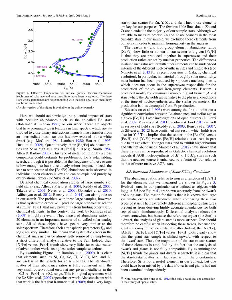
Figure 4 shows one version of the theoretical Hertzprung–Russell diagram using our derived stellar parameters effectivetemperature and surface gravity. It also shows several theoreticalisochrones of solar age (∼4.5 Gyr) and solar metallicity.Although different isochrones have different definitions of solarmetallicity, the differences are small and not important for ourpurposes. Isochrones computed by the following groups areshown in Figure 4, ordered by their hottest isochrone point(coolest is last in this list): Worthey (1994); Bertelli et al. (1994);Dotter et al. (2008); Pietrinferni et al. (2004); Yi et al. (2001).There are important differences between them, but collectivelythey can help us discard a few stars based on a zeroth-order ageestimate.

Determining ages of individual stars is a very difficulttask, particularly for stars on the main sequence, but a quickinspection of Figure 4 clearly shows that three of our samplestars cannot have solar age within any reasonable uncertainties.Stars HD 199881 and HD 207164 are too warm given the turnoffTeff of the solar-age, solar-metallicity isochrone, which is atmost ∼6300 K. Star HD 199951, on the other hand, appears tobe a giant star of younger age than solar. All of our other targets

6

http://www.as.utexas.edu/~ivan

http://kurucz.harvard.edu/linelists.html


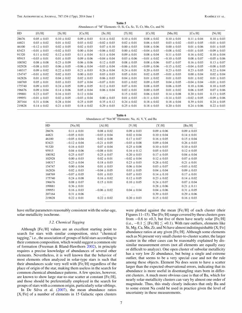
Table 5Abundances of “M” Elements: O, Si, Ca, Sc, Ti, Cr, Mn, Co, and Ni

HD [O/H] [Si/H] [Ca/H] [Sc/H] [Ti/H] [Cr/H] [Mn/H] [Co/H] [Ni/H]

28676 0.05 ± 0.03 0.10 ± 0.02 0.09 ± 0.03 0.14 ± 0.02 0.10 ± 0.01 0.08 ± 0.02 0.10 ± 0.01 0.11 ± 0.04 0.10 ± 0.0344821 0.03 ± 0.02 0.01 ± 0.02 0.03 ± 0.02 −0.02 ± 0.03 0.02 ± 0.01 0.06 ± 0.03 0.03 ± 0.02 −0.03 ± 0.05 −0.01 ± 0.0346100 −0.12 ± 0.03 0.02 ± 0.05 0.02 ± 0.03 0.07 ± 0.10 0.00 ± 0.03 0.08 ± 0.06 0.00 ± 0.03 0.01 ± 0.06 0.01 ± 0.0583423 −0.01 ± 0.03 −0.02 ± 0.03 0.00 ± 0.04 −0.06 ± 0.02 0.00 ± 0.02 −0.04 ± 0.03 −0.08 ± 0.02 −0.01 ± 0.05 −0.09 ± 0.0391320 0.11 ± 0.02 0.12 ± 0.03 0.11 ± 0.04 0.11 ± 0.04 0.09 ± 0.01 0.08 ± 0.04 0.11 ± 0.03 0.16 ± 0.02 0.10 ± 0.0495915 −0.03 ± 0.01 0.01 ± 0.05 0.09 ± 0.06 −0.04 ± 0.04 0.03 ± 0.06 −0.01 ± 0.02 −0.10 ± 0.05 0.08 ± 0.07 −0.05 ± 0.06100382 0.08 ± 0.08 0.23 ± 0.09 0.06 ± 0.06 0.12 ± 0.05 0.08 ± 0.05 0.08 ± 0.06 0.07 ± 0.07 0.16 ± 0.03 0.13 ± 0.07102928 −0.08 ± 0.03 0.06 ± 0.05 −0.06 ± 0.04 −0.03 ± 0.04 −0.06 ± 0.01 −0.09 ± 0.06 −0.15 ± 0.02 −0.04 ± 0.05 −0.08 ± 0.05148317 0.09 ± 0.02 0.22 ± 0.03 0.21 ± 0.03 0.26 ± 0.04 0.24 ± 0.01 0.20 ± 0.03 0.23 ± 0.03 0.23 ± 0.05 0.22 ± 0.04154747 −0.01 ± 0.02 0.02 ± 0.03 0.00 ± 0.03 0.03 ± 0.03 0.05 ± 0.01 0.02 ± 0.05 −0.01 ± 0.03 0.00 ± 0.04 0.02 ± 0.04162826 0.01 ± 0.02 0.04 ± 0.02 0.02 ± 0.03 0.06 ± 0.03 0.04 ± 0.01 0.01 ± 0.02 0.01 ± 0.03 0.01 ± 0.02 0.01 ± 0.03168769 0.05 ± 0.01 0.03 ± 0.03 0.07 ± 0.04 −0.07 ± 0.01 0.03 ± 0.02 0.09 ± 0.05 0.04 ± 0.05 −0.04 ± 0.04 −0.01 ± 0.03175740 0.09 ± 0.03 0.24 ± 0.05 0.09 ± 0.05 0.12 ± 0.03 0.07 ± 0.01 0.08 ± 0.05 0.06 ± 0.05 0.10 ± 0.06 0.10 ± 0.05196676 0.09 ± 0.04 0.14 ± 0.06 0.05 ± 0.04 0.06 ± 0.04 0.02 ± 0.01 0.00 ± 0.05 0.01 ± 0.02 0.06 ± 0.05 0.07 ± 0.06199881 0.23 ± 0.07 0.16 ± 0.03 0.12 ± 0.04 . . . 0.15 ± 0.02 0.06 ± 0.03 0.14 ± 0.08 0.20 ± 0.01 0.13 ± 0.05199951 −0.01 ± 0.03 0.02 ± 0.05 −0.03 ± 0.04 0.00 ± 0.03 0.01 ± 0.03 −0.11 ± 0.01 −0.14 ± 0.03 −0.02 ± 0.05 −0.09 ± 0.06207164 0.31 ± 0.06 0.28 ± 0.04 0.25 ± 0.05 0.35 ± 0.12 0.24 ± 0.02 0.18 ± 0.02 0.18 ± 0.04 0.39 ± 0.01 0.24 ± 0.05219828 0.14 ± 0.02 0.21 ± 0.03 0.18 ± 0.02 0.29 ± 0.03 0.25 ± 0.01 0.18 ± 0.03 0.20 ± 0.01 0.24 ± 0.06 0.22 ± 0.03

Table 6Abundances of “Not M” Elements: Na, Al, V, Y, and Ba

HD [Na/H] [Al/H] [V/H] [Y/H] [Ba/H]

28676 0.11 ± 0.01 0.08 ± 0.02 0.09 ± 0.03 0.09 ± 0.06 0.09 ± 0.0344821 −0.05 ± 0.01 −0.03 ± 0.04 0.02 ± 0.04 0.10 ± 0.04 0.14 ± 0.0146100 −0.05 ± 0.04 0.02 ± 0.08 0.17 ± 0.07 0.16 ± 0.05 0.15 ± 0.0483423 −0.12 ± 0.04 −0.21 ± 0.05 −0.03 ± 0.08 0.09 ± 0.04 0.26 ± 0.0391320 0.16 ± 0.03 0.07 ± 0.04 0.25 ± 0.08 0.10 ± 0.03 0.10 ± 0.0395915 0.04 ± 0.06 −0.08 ± 0.01 0.16 ± 0.12 0.05 ± 0.03 0.12 ± 0.05100382 0.25 ± 0.07 0.25 ± 0.07 0.20 ± 0.03 0.17 ± 0.05 0.04 ± 0.04102928 0.00 ± 0.03 0.02 ± 0.01 −0.02 ± 0.04 0.12 ± 0.03 0.07 ± 0.05148317 0.23 ± 0.04 0.18 ± 0.03 0.23 ± 0.03 0.28 ± 0.02 0.21 ± 0.01154747 0.00 ± 0.04 0.01 ± 0.03 0.06 ± 0.04 0.03 ± 0.07 −0.03 ± 0.02162826 0.02 ± 0.03 −0.04 ± 0.05 0.03 ± 0.05 0.04 ± 0.04 0.09 ± 0.03168769 −0.07 ± 0.05 0.01 ± 0.03 0.07 ± 0.03 0.14 ± 0.10 0.17 ± 0.01175740 0.24 ± 0.08 0.16 ± 0.02 0.12 ± 0.05 0.23 ± 0.02 0.14 ± 0.02196676 0.08 ± 0.07 0.15 ± 0.01 0.10 ± 0.05 0.24 ± 0.07 0.07 ± 0.04199881 0.36 ± 0.01 . . . . . . 0.28 ± 0.06 0.21 ± 0.11199951 0.16 ± 0.03 −0.06 ± 0.02 0.04 ± 0.04 0.04 ± 0.06 0.31 ± 0.05207164 0.31 ± 0.06 . . . . . . 0.39 ± 0.03 0.29 ± 0.06219828 0.22 ± 0.01 0.22 ± 0.02 0.20 ± 0.03 0.15 ± 0.02 0.16 ± 0.03

have stellar parameters reasonably consistent with the solar-age,solar-metallicity isochrone.

3.2. Chemical Tagging

Although [Fe/H] values are an excellent starting point tosearch for stars with similar composition, strict “chemicaltagging,” i.e., the association of groups of field stars according totheir common composition, which would suggest a common siteof formation (Freeman & Bland-Hawthorn 2002), in principlerequires a precise knowledge of abundances of several otherelements. Nevertheless, it is well known that the behavior ofmost elements often analyzed in solar-type stars is such thattheir abundances scale very well with [Fe/H] regardless of theplace of origin of the star, making them useless in the search forcommon chemical abundance patterns. A few species, however,are known to show large star-to-star scatter at constant [Fe/H],and those should be preferentially employed in the search forgroups of stars with a common origin, particularly solar siblings.

In De Silva et al. (2007), the mean abundance ratios[X/Fe] of a number of elements in 15 Galactic open clusters

were plotted against the mean [Fe/H] of each cluster (theirFigures 11–15). The [Fe/H] range covered by these clusters goesfrom −0.6 to +0.3, but five of them have nearly solar [Fe/H](i.e., −0.1 � [Fe/H] � +0.1). With rare outliers, elements likeSi, Mg, Ca, Mn, Zr, and Ni have almost indistinguishable [X/Fe]abundance ratios at any given [Fe/H]. Although some elementssuch as Ni present very small cluster-to-cluster scatter, the largerscatter in the other cases can be reasonably explained by dis-similar measurement errors (not all elements are equally easyor difficult to analyze). One open cluster of subsolar metallicityhas a very low Zr abundance, but being a single and extremeoutlier, that seems to be a very special case and not the ruleamong these objects. Element Na does seem to have a scatterlarger than the expected observational errors, indicating that itsabundance is more useful in disentangling stars born in differ-ent clusters. A much more obvious case is that of Ba, which fornearly solar-metallicity clusters can vary by almost one order ofmagnitude. Thus, this study clearly indicates that only Ba andto some extent Na could be used in practice given the level ofuncertainty in these measurements.

7


Figure 4. Effective temperature vs. surface gravity. Various theoreticalisochrones of solar age and solar metallicity have been overplotted. The threestars whose parameters are not compatible with the solar-age, solar-metallicityisochrone are labeled.


Here we should acknowledge the potential impact of starswith peculiar abundances such as the so-called Ba stars(Bidelman & Keenan 1951) on our work. These are objectsthat have prominent Ba ii features in their spectra, which are at-tributed to close binary interactions, namely mass transfer froman intermediate-mass star that has now evolved into a whitedwarf (e.g., McClure 1984; Lambert 1988; Han et al. 1995;Husti et al. 2009). Quantitatively, their [Ba/Fe] abundance ra-tios can be as high as 1 dex at [Fe/H] � 0 (e.g., Smith 1984;Allen & Barbuy 2006). This type of metal pollution by a closecompanion could certainly be problematic for a solar siblingsearch, although it is possible that the frequency of these eventsis low enough to have a relatively minor impact. Indeed, thestar-to-star scatter of the [Ba/Fe] abundance ratio observed inindividual open clusters is low and can be explained purely byobservational errors (De Silva et al. 2007).

Detailed chemical composition studies of large numbers offield stars (e.g., Allende Prieto et al. 2004; Reddy et al. 2003;Takeda et al. 2007; Neves et al. 2009; Gonzalez et al. 2010;Adibekyan et al. 2012; Bensby et al. 2014) can also guide usin our search. The problem with these large samples, however,is that systematic errors will produce large star-to-star scatterat similar [Fe/H] that may prevent us from finding other usefulchemical elements. In this context, the work by Ramırez et al.(2009) is highly relevant. They measured abundance ratios of20 elements in an important number of so-called solar analogstars. All of these objects have spectra very similar to thesolar spectrum. Therefore, their atmospheric parameters Teff andlog g are very similar. This means that systematic errors in thechemical analysis can be almost fully removed by employinga strict differential analysis relative to the Sun. Indeed, their[X/Fe] versus [Fe/H] trends show very little star-to-star scatterrelative to other works using less-strict sample selections.

By examining Figure 1 in Ramırez et al. (2009), it is clearthat elements such as Si, Ca, Sc, Ti, V, Cr, Mn, and Niare useless in the search for solar siblings. The star-to-starscatter of their abundance ratios is fully consistent with thevery small observational errors at any given metallicity in the−0.2 < [Fe/H] < +0.2 range. This is in good agreement withthe De Silva et al. (2007) open cluster work. Also consistent withthat work is the fact that Ramırez et al. (2009) find a very large

star-to-star scatter for Zn, Y, Zr, and Ba. Thus, those elementsare key for our purposes. The few available lines due to Zn andZr are blended in the majority of our sample stars. Although weare able to measure precise Zn and Zr abundances in the mostSun-like stars in our sample, we excluded these elements fromour work in order to maintain homogeneity in the analysis.

The reason α- and iron-group element abundance ratios[X/Fe] show little or no star-to-star scatter at a given [Fe/H]is that they are produced together in supernovae and theirproduction ratios are set by nuclear properties. The differencesin abundance ratio scatter with other elements can be understoodin terms of the different nucleosynthesis sites and timescales (seeNomoto et al. 2013 for a recent overview of Galactic chemicalevolution). In particular, in material of roughly solar metallicity,most barium has been produced by s-process nucleosynthesis,which does not occur in the supernovae responsible for theproduction of the α- and iron-group elements. Barium isproduced mostly by low-mass asymptotic giant branch (AGB)stars, where the Ba yields are sensitive to the physical conditionsat the time of nucleosynthesis and the stellar parameters; Baproduction is thus decoupled from Fe production.

Edvardsson et al. (1993) were among the first to point out asignificant correlation between Ba abundance and stellar age ata given [Fe/H]. Later investigations of open clusters (D’Oraziet al. 2009; Maiorca et al. 2011; Jacobson & Friel 2013) as wellas surveys of field stars (Reddy et al. 2003; Bensby et al. 2007;da Silva et al. 2012) have confirmed that result, which holds truealso for Y.15 This implies that the scatter in the [Ba/Fe] versus[Fe/H] and [Y/Fe] versus [Fe/H] relations is at least in partdue to an age effect. Younger stars tend to exhibit higher bariumand yttrium abundances. Maiorca et al. (2012) have shown thatthese trends can be reproduced in Galactic chemical evolutionmodels if AGB nucleosynthesis of M < 1.5 M� stars is suchthat the neutron source is enhanced by a factor of four relativeto that of more massive AGB stars.

3.3. Elemental Abundances of Solar Sibling Candidates

The abundance ratios relative to iron as a function of [Fe/H]for the elements that we measured are shown in Figure 5.Evolved stars, in our particular case defined as objects withlog g < 3.5 (see Figure 4), are shown separately from the dwarfsand subgiants. The reason for this is that it is known that largesystematic errors are introduced when comparing these twotypes of stars. Their extremely different atmospheric structuresprevent us from deriving highly accurate abundances for bothsets of stars simultaneously. Differential analysis reduces theerrors somewhat, but because the reference object (the Sun) isa dwarf, the analysis of giant stars is more suspect. One shouldtherefore be careful when inspecting these trends, because thegiant stars may introduce artificial scatter. Indeed, the [Na/Fe],[Al/Fe], [Si/Fe], and [Y/Fe] versus [Fe/H] plots clearly showthat the giant star sample is shifted upward with respect tothe dwarf stars. Thus, the magnitude of the star-to-star scatterof those elements is amplified by the fact that the analysis ofdwarfs and giants is not fully compatible. By examining the[Si/Fe] trends for giants and dwarfs separately, it is clear thatthe star-to-star scatter is in fact zero within the uncertainties.Therefore, Si is not a useful element in our context, but onecould have been misled by the data if dwarfs and giants had notbeen examined independently.

15 Note, however, that Yong et al. (2012) find only a weak Ba–age correlationin their study of open clusters.

8


Figure 5. Elemental abundance ratios relative to iron as a function of [Fe/H]. Evolved stars are shown with open squares; dwarfs and subgiants are represented byfilled circles. The dashed lines intersect at the solar values.


In good agreement with the open cluster and solar analogstudies, we find that most elements present a star-to-star scatterthat is fully compatible with the measurement errors. The excep-tions are the following species: Na, Al, V, Y, and Ba. Hereafter,all other elements are combined into a single indicator, M.

In Figure 6 we show elemental abundances relative to H,on a star-by-star basis, separating the important elements inour context (Na, Al, V, Y, and Ba) from M (the combinationof all other elements: O, Si, Ca, Sc, Ti, Cr, Mn, Co, and Ni).A star with the same composition as the Sun must have allvalues in Figure 6 around zero within the errors. Two starsstand out in this context: HD 154747 and HD 162826. Bothhave solar abundances within the errors, although the latterappears to have a slightly supersolar Ba abundance. Anotherinteresting object is HD 28676, which appears to have a +0.1offset in the abundances of all elements while retaining almostperfectly solar [X/Fe] abundance ratios. A similar pattern isexhibited by HD 93210, with the exception of its V abundance,which appears very high. The latter, however, could be due to anuncertain effective temperature (see below). From the chemicalstandpoint, these four objects are key solar sibling candidates.

3.4. Accounting for Systematic Errors

In Section 2.4 we described our method for deriving at-mospheric parameters using only measurements of iron linestrength on our high-resolution, high S/N spectra. Stellar prop-erties derived in this manner are often referred to as “spec-troscopic parameters.” Another common approach to derivingthe fundamental stellar parameters Teff and log g involves the

use of photometric data (colors) and measured trigonometricparallaxes. The former allow us to constrain Teff from color cal-ibrations based on less model-dependent techniques such as theinfrared flux method (IRFM) or even temperatures measureddirectly from known stellar angular diameters and bolometricfluxes. Parallaxes, on the other hand, allow us to calculate ab-solute magnitudes of stars, which can then be employed alongwith theoretical isochrones to compute the stellar masses andthus have another way of estimating log g. The stellar parametersthus derived are sometimes referred to as “physical parameters.”

In order to assess the impact of systematic errors in ourelemental abundance measurements, we rederived them usingphysical parameters, which were determined using the proce-dure outlined in Ramırez et al. (2013). Briefly, Teff was mea-sured using as many photometric colors as available and theIRFM Teff-color calibrations by Casagrande et al. (2010). Sur-face gravities were then inferred using the stars’ Hipparcos par-allaxes and the Yonsei–Yale isochrone grid (Yi et al. 2001; Kimet al. 2002). All four physical parameters, hereafter referred toas T ′

eff , log g′, [Fe/H]′, and v′t , were determined iteratively until

a final self-consistent solution was achieved, i.e., [Fe/H]′ and v′t

were recomputed by forcing the iron abundances to be indepen-dent of reduced equivalent width, but the excitation and ioniza-tion balance conditions were relaxed. Errors in T ′

eff correspondto the color-to-color scatter but weighted by the uncertainty ofeach color Teff calibration. The error in log g′ was estimatedfrom the width of the isochrone log g probability distribution(see Section 3.2 in Ramırez et al. 2013 for details). Finally, theuncertainty in [Fe/H]′ was computed by propagating the T ′

effand log g′ errors into the iron abundance calculations.

9


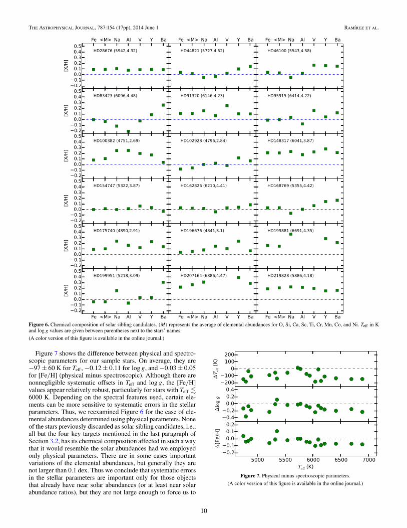
Figure 6. Chemical composition of solar sibling candidates. 〈M〉 represents the average of elemental abundances for O, Si, Ca, Sc, Ti, Cr, Mn, Co, and Ni. Teff in Kand log g values are given between parentheses next to the stars’ names.


Figure 7 shows the difference between physical and spectro-scopic parameters for our sample stars. On average, they are−97 ± 60 K for Teff , −0.12 ± 0.11 for log g, and −0.03 ± 0.05for [Fe/H] (physical minus spectroscopic). Although there arenonnegligible systematic offsets in Teff and log g, the [Fe/H]values appear relatively robust, particularly for stars with Teff �6000 K. Depending on the spectral features used, certain ele-ments can be more sensitive to systematic errors in the stellarparameters. Thus, we reexamined Figure 6 for the case of ele-mental abundances determined using physical parameters. Noneof the stars previously discarded as solar sibling candidates, i.e.,all but the four key targets mentioned in the last paragraph ofSection 3.2, has its chemical composition affected in such a waythat it would resemble the solar abundances had we employedonly physical parameters. There are in some cases importantvariations of the elemental abundances, but generally they arenot larger than 0.1 dex. Thus we conclude that systematic errorsin the stellar parameters are important only for those objectsthat already have near solar abundances (or at least near solarabundance ratios), but they are not large enough to force us to

Figure 7. Physical minus spectroscopic parameters.


10


reconsider the other targets in our sample as potentially truesolar siblings.

In addition to the potential systematic errors introducedby model parameter uncertainties, it is worth mentioning thepossibility that the photospheric composition of stars may beaffected by planet formation processes. Melendez et al. (2009)have found that, relative to the majority of solar twin stars, theSun is deficient in refractory elements by about 0.08 dex. Theyattribute this deficiency to the fact that the Sun formed rockyplanets, which retained those metals during the formation of thesolar system. Similarly, Ramırez et al. (2011) have found that thesecondary star in the 16 Cyg binary system, which hosts a gasgiant planet, is metal-poor relative to the primary, which doesnot appear to have substellar mass companions (Cochran et al.1997). The observed metallicity difference of about 0.04 dex(volatiles and refractories are equally depleted in this case) isalso attributed to the formation of the planet, in this case a gasgiant.

It is important to point out that other authors have foundresults that conflict with the ones described above. In particular,based on an analysis of a stellar sample with a known planetpopulation, Gonzalez Hernandez et al. (2010, 2013) arguethat the connection to planet formation processes is weak,although their exoplanet host sample is admittedly biased towardmassive planets whereas the Melendez et al. hypothesis concernsrocky bodies. In any case, one should keep in mind thatthe chemical abundance anomalies are still present, and thatregardless of their interpretation, they do introduce systematicuncertainties in our context. Similarly, Schuler et al. (2011) havefound no differences in chemical composition between the twocomponents of the 16 Cyg binary system. While this discrepancywith the Ramırez et al. results remains unresolved, anotherstudy, which employed much higher quality data for these starsand independent measurements of the spectral features, hasconfirmed the slightly dissimilar chemical composition of the16 Cyg stars (Tucci Maia et al. 2014).

From the discussion above, a conservative estimate of our[X/Fe] errors, including model systematics and the potentialimpact of planet formation on the surface composition of stars, is�0.1 dex. The line-to-line scatter values listed in Tables 5 and 6are not the dominant source of uncertainty for most elements.

3.5. Key Targets

In Section 3.2 we listed four key targets for siblings of the Sunbased on the similarity of their metal abundance ratios to thesolar abundances. They are HD 28676, HD 91320, HD 154747,and HD 162826. As will be explained in Section 3.6, HD 83423is another interesting candidate, but purely on a dynamical basis.We add this star to our list of key targets to emphasize certainpoints of our discussion.

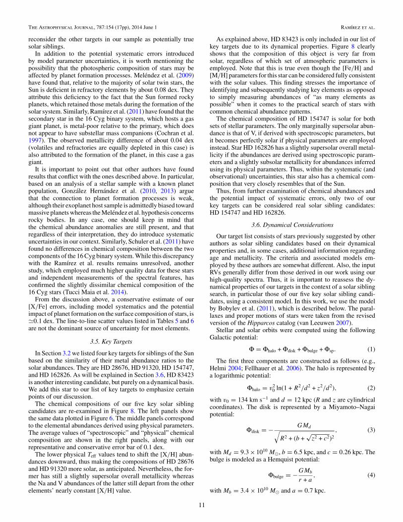
The chemical compositions of our five key solar siblingcandidates are re-examined in Figure 8. The left panels showthe same data plotted in Figure 6. The middle panels correspondto the elemental abundances derived using physical parameters.The average values of “spectroscopic” and “physical” chemicalcomposition are shown in the right panels, along with ourrepresentative and conservative error bar of 0.1 dex.

The lower physical Teff values tend to shift the [X/H] abun-dances downward, thus making the compositions of HD 28676and HD 91320 more solar, as anticipated. Nevertheless, the for-mer has still a slightly supersolar overall metallicity whereasthe Na and V abundances of the latter still depart from the otherelements’ nearly constant [X/H] value.

As explained above, HD 83423 is only included in our list ofkey targets due to its dynamical properties. Figure 8 clearlyshows that the composition of this object is very far fromsolar, regardless of which set of atmospheric parameters isemployed. Note that this is true even though the [Fe/H] and[M/H] parameters for this star can be considered fully consistentwith the solar values. This finding stresses the importance ofidentifying and subsequently studying key elements as opposedto simply measuring abundances of “as many elements aspossible” when it comes to the practical search of stars withcommon chemical abundance patterns.

The chemical composition of HD 154747 is solar for bothsets of stellar parameters. The only marginally supersolar abun-dance is that of V, if derived with spectroscopic parameters, butit becomes perfectly solar if physical parameters are employedinstead. Star HD 162826 has a slightly supersolar overall metal-licity if the abundances are derived using spectroscopic param-eters and a slightly subsolar metallicity for abundances inferredusing its physical parameters. Thus, within the systematic (andobservational) uncertainties, this star also has a chemical com-position that very closely resembles that of the Sun.

Thus, from further examination of chemical abundances andthe potential impact of systematic errors, only two of ourkey targets can be considered real solar sibling candidates:HD 154747 and HD 162826.

3.6. Dynamical Considerations

Our target list consists of stars previously suggested by otherauthors as solar sibling candidates based on their dynamicalproperties and, in some cases, additional information regardingage and metallicity. The criteria and associated models em-ployed by these authors are somewhat different. Also, the inputRVs generally differ from those derived in our work using ourhigh-quality spectra. Thus, it is important to reassess the dy-namical properties of our targets in the context of a solar siblingsearch, in particular those of our five key solar sibling candi-dates, using a consistent model. In this work, we use the modelby Bobylev et al. (2011), which is described below. The paral-laxes and proper motions of stars were taken from the revisedversion of the Hipparcos catalog (van Leeuwen 2007).

Stellar and solar orbits were computed using the followingGalactic potential:

Φ = Φhalo + Φdisk + Φbulge + Φsp. (1)

The first three components are constructed as follows (e.g.,Helmi 2004; Fellhauer et al. 2006). The halo is represented bya logarithmic potential:

Φhalo = v20 ln(1 + R2/d2 + z2/d2), (2)

with v0 = 134 km s−1 and d = 12 kpc (R and z are cylindricalcoordinates). The disk is represented by a Miyamoto–Nagaipotential:

Φdisk = − GMd√R2 + (b +

√z2 + c2)2

, (3)

with Md = 9.3 × 1010 M�, b = 6.5 kpc, and c = 0.26 kpc. Thebulge is modeled as a Hemquist potential:

Φbulge = −GMb

r + a, (4)

with Mb = 3.4 × 1010 M� and a = 0.7 kpc.

11


Figure 8. Chemical composition of our five key solar sibling candidates. Each row corresponds to one star, whose name is provided in the right-most panel. Leftpanels: as in Figure 6, i.e., elemental abundances obtained using spectroscopic parameters. Middle panels: as in the left panels, but for elemental abundances derivedusing physical parameters. Right panels: average of “spectroscopic” and “physical” abundances. 〈M〉 represents the average of elemental abundances for O, Si, Ca,Sc, Ti, Cr, Mn, Co, and Ni. An error bar of 0.1 dex, which we estimate as a conservative uncertainty for our abundances, including systematics, is also shown in thesepanels.


The following spiral wave component makes this Galacticgravitational potential model more realistic (Fernandez et al.2008):

Φsp = A cos[m(Ωpt − θ ) + χ (R)], (5)

where

A = (R0Ω0)2fr0 tan i

m, (6)

and

χ (R) = − m

tan iln

(R

R0

)+ χ�. (7)

Our adopted spiral wave parameters are pitch angle i =−12◦, number of arms m = 4, phase of Sun χ0 = −120◦,strength fr0 = 0.05, and velocity of spiral pattern Ωp =20 km s−1 kpc−1. The circular speed at the solar radius(R� = 8.0 kpc) is 220 km s−1, and the peculiar solar velocitiesare (U�, V�,W� = 10, 11, 7) km s−1 (Bobylev & Bajkova2010; Schonrich et al. 2010).

The model described above allows us to compute encounterparameters between the stellar and solar orbit in the past. Inparticular, we can calculate the relative distance d and velocity

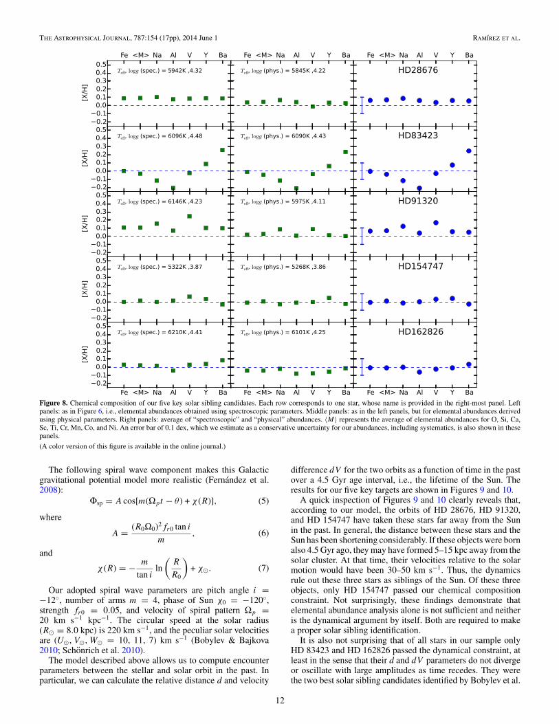
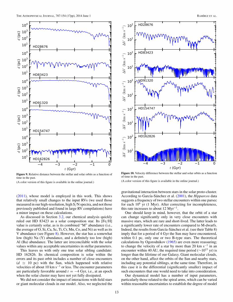
difference dV for the two orbits as a function of time in the pastover a 4.5 Gyr age interval, i.e., the lifetime of the Sun. Theresults for our five key targets are shown in Figures 9 and 10.

A quick inspection of Figures 9 and 10 clearly reveals that,according to our model, the orbits of HD 28676, HD 91320,and HD 154747 have taken these stars far away from the Sunin the past. In general, the distance between these stars and theSun has been shortening considerably. If these objects were bornalso 4.5 Gyr ago, they may have formed 5–15 kpc away from thesolar cluster. At that time, their velocities relative to the solarmotion would have been 30–50 km s−1. Thus, the dynamicsrule out these three stars as siblings of the Sun. Of these threeobjects, only HD 154747 passed our chemical compositionconstraint. Not surprisingly, these findings demonstrate thatelemental abundance analysis alone is not sufficient and neitheris the dynamical argument by itself. Both are required to makea proper solar sibling identification.

It is also not surprising that of all stars in our sample onlyHD 83423 and HD 162826 passed the dynamical constraint, atleast in the sense that their d and dV parameters do not divergeor oscillate with large amplitudes as time recedes. They werethe two best solar sibling candidates identified by Bobylev et al.

12


Figure 9. Relative distance between the stellar and solar orbits as a function oftime in the past.


(2011), whose model is employed in this work. This showsthat relatively small changes to the input RVs (we used thosemeasured in our high-resolution, high S/N spectra, and not thosepreviously published and found in large RV compilations) havea minor impact on these calculations.

As discussed in Section 3.2, our chemical analysis quicklyruled out HD 83423 as a solar composition star. Its [Fe/H]value is certainly solar, as is its combined “M” abundance (i.e.,the average of O, Si, Ca, Sc, Ti, Cr, Mn, Co, and Ni) as well as itsV abundance (see Figure 8). However, the star has a somewhatlow (high) Na (Y) abundance, and a definitely too low (high)Al (Ba) abundance. The latter are irreconcilable with the solarvalues within any acceptable uncertainties in stellar parameters.

This leaves us with only one true solar sibling candidate:HD 162826. Its chemical composition is solar within theerrors and its past orbit includes a number of close encounters(d � 10 pc) with the Sun, which happened with relativevelocities of about 10 km s−1 or less. The encounter parametersare particularly favorable around t = −4 Gyr, i.e., at an epochwhen the solar cluster may have not yet fully dissipated.

We did not consider the impact of interactions with field starsor giant molecular clouds in our model. Also, we neglected the

Figure 10. Velocity difference between the stellar and solar orbits as a functionof time in the past.


gravitational interaction between stars in the solar proto-cluster.According to Garcıa-Sanchez et al. (2001), the Hipparcos datasuggests a frequency of two stellar encounters within one parsecfor each 106 yr (1 Myr). After correcting for incompleteness,this rate increases to about 12 Myr−1.

One should keep in mind, however, that the orbit of a starcan change significantly only in very close encounters withmassive stars, which are rare and short-lived. The latter leads toa significantly lower rate of encounters compared to M-dwarfs.Indeed, the results from Garcıa-Sanchez et al. (see their Table 8)imply that for a period of 4 Gyr the Sun may have encountered,within 0.1 pc, only one or two B-type stars. The theoreticalcalculations by Ogorodnikov (1965) are even more reassuring;to change the velocity of a star by more than 20 km s−1 in anencounter within 40 AU, the required time period (∼1013 yr) islonger than the lifetime of our Galaxy. Giant molecular clouds,on the other hand, affect the orbits of the Sun and nearby stars,including any potential siblings, at the same time. Therefore, inthis case it is the differential (significantly smaller) impact ofsuch encounters that one would need to take into consideration.

Our dynamical model has a number of input parameters,particularly those related to the spiral arms, which can be variedwithin reasonable uncertainties to establish the degree of model

13


Table 7Rare Earth Element Abundances

Species Wavelength EP log gf log gf hfs/IS log ε log ε log ε

(Å) (eV) Reference Reference Sun HD 162826a HD 162826b

La ii 4662.50 0.000 −1.24 1 2 1.10 1.15 1.074748.73 0.927 −0.54 1 1.16 1.26 1.175303.53 0.321 −1.35 1 2 1.12 1.25 1.146390.48 0.321 −1.41 1 2 1.18 1.23 1.13

Ce ii 4486.91 0.295 −0.18 3 1.73 1.76 1.664523.08 0.516 −0.08 3 1.58 1.68 1.564562.36 0.478 +0.21 3 1.61 1.68 1.584628.16 0.516 +0.14 3 1.59 1.66 1.545187.46 1.212 +0.17 3 1.59 1.65 1.555330.56 0.869 −0.40 3 1.67 1.72 1.62

Nd ii 4446.38 0.205 −0.35 4 5 1.32 1.44 1.325234.19 0.550 −0.51 4 1.46 1.53 1.435319.81 0.550 −0.14 4 1.34 1.37 1.30

Sm ii 4467.34 0.659 +0.15 6 5 0.88 1.00 0.904519.63 0.544 −0.35 6 0.94 1.07 0.964537.94 0.485 −0.48 6 5 0.97 1.09 0.974676.90 0.040 −0.87 6 0.89 1.09 0.97

Notes.a Spectroscopic model parameters.b Physical model parameters.References. (1) Lawler et al. 2001; (2) Ivans et al. 2006; (3) Lawler et al. 2009; (4) Den Hartog et al. 2003; (5) Roederer et al. 2008; (6) Lawler et al.2006.

dependency of our results. Given the demanding nature of thesecomputations, we restricted them to two of our stars: HD 154747and HD 162826, i.e., the two stars that have solar chemicalcomposition. Orbit calculations were made with two and fourarms, varying the pitch angle from −10◦ to −14◦ for the four-arm model and from −5◦ to −7◦ for the two-arm model. Thephase of the Sun relative to the spiral arm was varied from−90◦ to −140◦, and the pattern speed was varied from 10 to24 km s−1 kpc−1. The total number of models computed is 900for each star.

For HD 162826 we obtained past close encounters (d <100 pc, ΔV < 50 km s−1, t < −3 Gyr) in 64% of the models.On the other hand, HD 154747 shows this type of encounterin only 1.3% of the models. Thus, within reasonable modeluncertainty, HD 162826 remains a good dynamical solar siblingcandidate, whereas it remains highly unlikely that HD 154747was born near the Sun.

3.7. Abundances of Trace Elements in HD 162826

We use several of the rare earth elements to further testwhether HD 162826 meets our chemical criteria for being asolar sibling. In solar-type stars, these elements owe their originto both r-process and s-process neutron-capture reactions, whichreflect a different set of chemical evolution clocks than thelighter elements. We identify 17 lines of four species that areunblended in our spectra of the Sun and HD 162826. Theselines are listed in Table 7. Abundances of La ii, Ce ii, Nd ii,and Sm ii are derived from spectrum synthesis using MOOG.Line lists were constructed using the Kurucz & Bell (1995)lists, using updated log gf values from recent laboratory studieswhen possible. We adjust the line strengths to reproduce thesolar spectrum and then use these lists without change forthe analysis of HD 162826. Table 7 lists the wavelength, EP,and log gf value for each transition, although the transitionprobabilities cancel out in a differential analysis. Our syntheses

Table 8Mean Line-by-line Rare Earth Element Abundance Differences

Species No. Lines HD 162826a − Sun HD 162826b − Sun

〈Δ〉 σ σμ 〈Δ〉 σ σμ

La ii 4 +0.083 0.039 0.020 −0.013 0.033 0.017Ce ii 6 +0.063 0.023 0.010 −0.043 0.018 0.007Nd ii 3 +0.073 0.045 0.026 −0.023 0.021 0.012Sm ii 4 +0.143 0.039 0.019 +0.030 0.035 0.017

Notes.a Spectroscopic model parameters.b Physical model parameters.

account for hyperfine splitting (hfs) and isotope shifts (IS) forseveral of these lines. We adopt the solar isotopic fractions givenby Lodders (2003) for the Sun and HD 162826. The derivedabundances are listed in Table 7. Table 8 lists the mean line-by-line differential abundances between the Sun and HD 162826.Two sets of values are given, one using the set of spectroscopicmodel atmosphere parameters for HD 162826 and one using theset of physical values.

Using spectroscopic parameters, the La, Ce, and Nd are verysimilar to the Ba abundance, i.e., slightly supersolar (� +0.08).However, using physical parameters, all of these elements havesolar abundances in HD 162826 within the internal error. TheSm abundance is also solar within the errors if we employthe physical parameters but supersolar at +0.14 dex usingspectroscopic parameters. The average of these abundances(excluding Sm), as derived using both sets of parameters, isabout +0.02 dex, i.e., solar within both systematic and internalerrors. Of all elements studied in this work for HD 162826,only Sm appears to depart from the solar abundances, witha spectroscopic/physical average value of +0.09. However,considering our conservative estimate of 0.1 dex of systematic

14


Figure 11. Relative radial velocity as a function of Julian Date for HD 162826.The radial velocities in this plot are given with respect to the weighted mean ofall observed values.


error, this value may be marginally consistent with the solar Smabundance.

3.8. High-precision Radial Velocity Data for HD 162826

Star HD 162826 is included in the target sample of 250 F-,G-, K-, and M-type stars of the McDonald Observatory planetsearch program at the Harlan J. Smith 2.7 m Telescope (e.g.,Cochran et al. 1997; Endl et al. 2004; Robertson et al. 2012).This long-term RV survey is designed to probe the populationof gas giant planets beyond the ice line at several AU. Suchplanets presumably have not migrated inward from the locationof their formation. Figure 11 displays the 15 yr of precise RVmeasurements of HD 162826. The 50 RV data points have anoverall rms scatter of 6.0 m s−1 and an average error of 5.4 m s−1.The star is constant at the 6 m s−1 level and does not seem tohave a massive planetary companion with a period of <15 yr.Also, there is no clear evidence of binarity.

We computed the upper limits on detectable planets in theRV data for HD 162826. The detection limit was determined byadding a fictitious Keplerian signal to the data, then attemptingto recover it via a generalized Lomb–Scargle periodogram(Zechmeister & Kurster 2009). Here, we have assumed circularorbits; for each combination of period P and RV semiamplitudeK, we tried 30 values of orbital phase. A planet is deemeddetectable if 99% of orbital configurations at a given P and Kare recovered with a false-alarm probability (Sturrock & Scargle2010) of less than 1%. This approach is essentially identical tothat used in the work by Wittenmyer et al. (2006, 2010, 2011b).The resulting mass limits are shown in Figure 12. Clearly, hotJupiters, i.e., planets with masses comparable to that of Jupiterin short-period orbits, can be ruled out.

To determine the probability that an undetected Jupiter-mass planet orbits HD 162826, we repeated the detectabilitysimulations described above for a range of recovery rates(10%–90%) as in Wittenmyer et al. (2011a). For a Jupiter-mass planet in a Jupiter-like (12 yr) circular orbit, we estimatea 35% probability that such a planet is present based on thenondetection from our RV data.

4. CONCLUSIONS

Detailed elemental abundance analysis and proper chemicaltagging are both required in the search for the stars that were

Figure 12. Mass limits for single planets in circular orbits around HD 162826.Planets with parameters in the region above the solid line would have beenrecovered with 99% probability at a false-alarm-probability of less than 1%.


born together with the Sun. However, one should keep inmind that not all elements are equally important. Althoughderiving abundances of “as many elements as possible” wouldbe ideal, in practice one could concentrate on a few keyelements as an intermediate step between employing onlyphotometric metallicities and a very detailed high-precisionchemical analysis. In particular, the spectral lines due to Baare very strong, hence easily measured in medium-resolutionspectra. Moreover, the large star-to-star dispersion observedin the [Ba/Fe] versus [Fe/H] plane suggests that the Baabundance is highly sensitive to the place of origin of stars.A perfectly reasonable intermediate step would therefore be themeasurement of Fe and Ba abundances in medium-resolution,moderately high S/N spectra.

Only the star HD 162826 (HR 6669, HIP 87382) satisfies bothour dynamical and chemical criteria for being a true sibling ofthe Sun. This object, a late F-type dwarf star located at about34 pc (∼110 lt-yr) from the Sun in the constellation Hercules, isbright (V = 6.7) and easily observable with small- and medium-sized telescopes. High-precision RV observations carried outover a period of time longer than 15 yr rule out the presence ofhot-Jupiter planets. These data also suggest a two-thirds chancethat a Jupiter analog is not present either. Smaller terrestrialplanets cannot be ruled out at this moment.

The mass of HD 162826, estimated from the location ofthe star on the Hertzsprung–Russell diagram compared toYonsei–Yale isochrones (as in Ramırez et al. 2013), is 1.15 M�.If this star were the only solar sibling in the 1.1–1.2 M� range,the Salpeter (1955) initial mass function would suggest theexistence of other ∼400 solar siblings of mass greater than0.1 M� dispersed throughout the Galaxy. Because the number ofstars in the solar cluster is estimated to be 103–104, this impliesthat there should be just a few other solar siblings of ∼1 M�present in the solar neighborhood. On the other hand, this meansthat there are a few hundred M-dwarfs that are also siblings ofthe Sun within 100 pc. Unfortunately, the detailed chemicalcomposition analysis of M-dwarfs that would be required toidentify them is currently beyond our capabilities.

The combination of astrometric data from the ongoing Gaiamission and spectroscopic data from surveys of comparablelarge size such as the ESO-Gaia survey, Apache Point GalacticEvolution Experiment (APOGEE), or GALAH will allow us to

15


discover many more solar siblings in a very near future. Weexpect that the analysis presented in this paper will guide futureendeavors in this field and allow us to perform these searchesmore efficiently.

I.R. acknowledges support from NASA’s Sagan FellowshipProgram to conduct most of the observations presented in thispaper. A.T.B and V.V.B.’s work is supported by the “Nonsta-tionary Phenomena in Objects of the Universe” Programmeof the Presidium of the Russian Academy of Sciences andthe “Multiwavelength Astrophysical Research” grant no. NSh-16245.2012.2 from the President of the Russian Federation.D.L.L. thanks the Robert A. Welch Foundation of Houston,Texas for support through grant F-634. The McDonald Obser-vatory exoplanet survey is currently supported by the NationalScience Foundation under grant AST #1313075. Previous sup-port for this project was given by the National Aeronautics andSpace Agency through the Origins of Solar Systems Programgrants NNX07AL70G, NNX09AB30G, and NNX10AL60G.

REFERENCES

Adams, F. C. 2010, ARA&A, 48, 47Adams, F. C., & Spergel, D. N. 2005, AsBio, 5, 497Adibekyan, V. Z., Sousa, S. G., Santos, N. C., et al. 2012, A&A, 545, A32Allen, C., & Santillan, A. 1991, RMxAA, 22, 255Allen, D. M., & Barbuy, B. 2006, A&A, 454, 895Allende Prieto, C., Barklem, P. S., Lambert, D. L., & Cunha, K. 2004, A&A,

420, 183Batista, S. F. A., Adibekyan, V. Z., Sousa, S. G., et al. 2014, A&A, 564, A43Batista, S. F. A., & Fernandes, J. 2012, NewA, 17, 514Belbruno, E., Moro-Martın, A., Malhotra, R., & Savransky, D. 2012, AsBio,

12, 754Bensby, T., Feltzing, S., & Oey, M. S. 2014, A&A, 562, A71Bensby, T., Zenn, A. R., Oey, M. S., & Feltzing, S. 2007, ApJL, 663, L13Bernstein, R., Shectman, S. A., Gunnels, S. M., Mochnacki, S., & Athey, A. E.

2003, SPIE, 4841, 1694Bertelli, G., Bressan, A., Chiosi, C., Fagotto, F., & Nasi, E. 1994, A&AS,

106, 275Bidelman, W. P., & Keenan, P. C. 1951, ApJ, 114, 473Bland-Hawthorn, J., Krumholz, M. R., & Freeman, K. 2010, ApJ, 713, 166Bobylev, V. V., & Bajkova, A. T. 2010, MNRAS, 408, 1788Bobylev, V. V., Bajkova, A. T., & Myllari, A. A. 2010, AstL, 36, 27Bobylev, V. V., Bajkova, A. T., Myllari, A., & Valtonen, M. 2011, AstL, 37, 550Bouvier, A., & Wadhwa, M. 2010, NatGe, 3, 637Bressert, E., Bastian, N., Gutermuth, R., et al. 2010, MNRAS, 409, L54Brown, A. G. A., Portegies Zwart, S. F., & Bean, J. 2010, MNRAS, 407, 458Brown, M. E., Trujillo, C., & Rabinowitz, D. 2004, ApJ, 617, 645Casagrande, L., Ramırez, I., Melendez, J., Bessell, M., & Asplund, M.

2010, A&A, 512, 54Casagrande, L., Schonrich, R., Asplund, M., et al. 2011, A&A, 530, A138Cayrel de Strobel, G., Soubiran, C., & Ralite, N. 2001, A&A, 373, 159Chubak, C., Marcy, G., Fischer, D. A., et al. 2012, arXiv:1207.6212Cochran, W. D., Hatzes, A. P., Butler, R. P., & Marcy, G. W. 1997, ApJ,

483, 457da Silva, L., Girardi, L., Pasquini, L., et al. 2006, A&A, 458, 609da Silva, R., Porto de Mello, G. F., Milone, A. C., et al. 2012, A&A, 542, A84De Silva, G. M., Freeman, K. C., Bland-Hawthorn, J., Asplund, M., & Bessell,

M. S. 2007, AJ, 133, 694Demarque, P., Green, E. M., & Guenther, D. B. 1992, AJ, 103, 151Den Hartog, E. A., Lawler, J. E., Sneden, C., & Cowan, J. J. 2003, ApJS,

148, 543D’Orazi, V., Magrini, L., Randich, S., et al. 2009, ApJL, 693, L31Dotter, A., Chaboyer, B., Jevremovic, D., et al. 2008, ApJS, 178, 89Edvardsson, B., Andersen, J., Gustafsson, B., et al. 1993, A&A, 275, 101Endl, M., Hatzes, A. P., Cochran, W. D., et al. 2004, ApJ, 611, 1121Epstein, C. R., Johnson, J. A., Dong, S., et al. 2010, ApJ, 709, 447Evans, N. J., II, Dunham, M. M., Jørgensen, J. K., et al. 2009, ApJS, 181, 321Fellhauer, M., Belokurov, V., Evans, N. W., et al. 2006, ApJ, 651, 167Feltzing, S., Holmberg, J., & Hurley, J. R. 2001, A&A, 377, 911Fernandez, D., Figueras, F., & Torra, J. 2008, A&A, 480, 735Freeman, K., & Bland-Hawthorn, J. 2002, ARA&A, 40, 487

Garcıa-Sanchez, J., Weissman, P. R., Preston, R. A., et al. 2001, A&A, 379, 634Gilmore, G., Randich, S., Asplund, M., et al. 2012, Msngr, 147, 25Gonzalez, G., Carlson, M. K., & Tobin, R. W. 2010, MNRAS, 407, 314Gonzalez Hernandez, J. I., Delgado-Mena, E., Sousa, S. G., et al. 2013, A&A,

552, A6Gonzalez Hernandez, J. I., Israelian, G., Santos, N. C., et al. 2010, ApJ,

720, 1592Goswami, J. N., & Vanhala, H. A. T. 2000, in Protostars and Planets IV, ed. V.

Mannings, A. P. Boss, & S. S. Russell (Tucson, AZ: Univ. Arizona Press),963

Gustafsson, B., Edvardsson, B., Eriksson, K., et al. 2008, A&A, 486, 951Han, Z., Eggleton, P. P., Podsiadlowski, P., & Tout, C. A. 1995, MNRAS,

277, 1443Helmi, A. 2004, ApJL, 610, L97Holmberg, J., Nordstrom, B., & Andersen, J. 2007, A&A, 475, 519Holmberg, J., Nordstrom, B., & Andersen, J. 2009, A&A, 501, 941Husti, L., Gallino, R., Bisterzo, S., Straniero, O., & Cristallo, S. 2009, PASA,

26, 176Ivans, I. I., Simmerer, J., Sneden, C., et al. 2006, ApJ, 645, 613Jacobson, H. R., & Friel, E. D. 2013, AJ, 145, 107Janes, K. A., Tilley, C., & Lynga, G. 1988, AJ, 95, 771Johnson, H. L., & Sandage, A. R. 1955, ApJ, 121, 616Kim, Y., Demarque, P., Yi, S. K., & Alexander, D. R. 2002, ApJS, 143, 499Kurucz, R., & Bell, B. 1995, Atomic Line Data Kurucz CD-ROM No. 23.

(Cambridge, MA: Smithsonian Astrophysical Observatory)Lada, C. J., & Lada, E. A. 2003, ARA&A, 41, 57Lambert, D. L. 1988, in IAU Symp. 132, The Impact of Very High S/N

Spectroscopy on Stellar Physics, ed. G. Cayrel de Strobel & M. Spite(Dordrecht: Kluwer), 563

Lawler, J. E., Den Hartog, E. A., Sneden, C., & Cowan, J. J. 2006, ApJS,162, 227

Lawler, J. E., Sneden, C., Cowan, J. J., Ivans, I. I., & Den Hartog, E. A.2009, ApJS, 182, 51

Lawler, J. E., Wickliffe, M. E., den Hartog, E. A., & Sneden, C. 2001, ApJ,563, 1075

Lin, C. C., Yuan, C., & Shu, F. H. 1969, ApJ, 155, 721Lindegren, L., Lammers, U., Hobbs, D., et al. 2012, A&A, 538, A78Lodders, K. 2003, ApJ, 591, 1220Looney, L. W., Tobin, J. J., & Fields, B. D. 2006, ApJ, 652, 1755Maiorca, E., Magrini, L., Busso, M., et al. 2012, ApJ, 747, 53Maiorca, E., Randich, S., Busso, M., Magrini, L., & Palmerini, S. 2011, ApJ,

736, 120McClure, R. D. 1984, PASP, 96, 117Melendez, J., Asplund, M., Gustafsson, B., & Yong, D. 2009, ApJL, 704, L66Melendez, J., & Ramırez, I. 2007, ApJL, 669, L89Mishurov, Y. N., & Acharova, I. A. 2011, MNRAS, 412, 1771Miyamoto, M., & Nagai, R. 1975, PASJ, 27, 533Monroe, T. R., Melendez, J., Ramırez, I., et al. 2013, ApJL, 774, L32Morbidelli, A., & Levison, H. F. 2004, AJ, 128, 2564Neves, V., Santos, N. C., Sousa, S. G., Correia, A. C. M., & Israelian, G.

2009, A&A, 497, 563Nomoto, K., Kobayashi, C., & Tominaga, N. 2013, ARA&A, 51, 457Nordstrom, B., Mayor, M., Andersen, J., et al. 2004, A&A, 418, 989Ogorodnikov, K. F. 1965, Dynamics of Stellar Systems (Oxford: Pergamon

Press)Onehag, A., Gustafsson, B., & Korn, A. 2014, A&A, 562, A102Onehag, A., Korn, A., Gustafsson, B., Stempels, E., & Vandenberg, D. A.

2011, A&A, 528, A85Paczynski, B. 1990, ApJ, 348, 485Pasquini, L., Biazzo, K., Bonifacio, P., Randich, S., & Bedin, L. R. 2008, A&A,

489, 677Perryman, M. A. C., Lindegren, L., Kovalevsky, J., et al. 1997, A&A, 323, L49Pfalzner, S. 2013, A&A, 549, A82Pichardo, B., Moreno, E., Allen, C., et al. 2012, AJ, 143, 73Pietrinferni, A., Cassisi, S., Salaris, M., & Castelli, F. 2004, ApJ, 612, 168Porras, A., Christopher, M., Allen, L., et al. 2003, AJ, 126, 1916Portegies Zwart, S. F. 2009, ApJL, 696, L13Porto de Mello, G. F., & da Silva, L. 1997, ApJL, 482, L89Ramırez, I., Allende Prieto, C., & Lambert, D. L. 2007, A&A, 465, 271Ramırez, I., Allende Prieto, C., & Lambert, D. L. 2013, ApJ, 764, 78Ramırez, I., Melendez, J., & Asplund, M. 2009, A&A, 508, L17Ramırez, I., Melendez, J., Cornejo, D., Roederer, I. U., & Fish, J. R. 2011, ApJ,

740, 76Randich, S., Sestito, P., Primas, F., Pallavicini, R., & Pasquini, L. 2006, A&A,

450, 557Reddy, B. E., Tomkin, J., Lambert, D. L., & Allende Prieto, C. 2003, MNRAS,

340, 304

16

http://dx.doi.org/10.1146/annurev-astro-081309-130830

http://adsabs.harvard.edu/abs/2010ARA&A..48...47A

http://adsabs.harvard.edu/abs/2010ARA&A..48...47A

http://dx.doi.org/10.1089/ast.2005.5.497

http://adsabs.harvard.edu/abs/2005AsBio...5..497A

http://adsabs.harvard.edu/abs/2005AsBio...5..497A

http://dx.doi.org/10.1051/0004-6361/201219401

http://adsabs.harvard.edu/abs/2012A&A...545A..32A

http://adsabs.harvard.edu/abs/2012A&A...545A..32A

http://adsabs.harvard.edu/abs/1991RMxAA..22..255A

http://adsabs.harvard.edu/abs/1991RMxAA..22..255A

http://dx.doi.org/10.1051/0004-6361:20064912

http://adsabs.harvard.edu/abs/2006A&A...454..895A


http://dx.doi.org/10.1051/0004-6361:20035801



http://dx.doi.org/10.1051/0004-6361/201423645

http://adsabs.harvard.edu/abs/2014A&A...564A..43B


http://dx.doi.org/10.1016/j.newast.2011.12.001

http://adsabs.harvard.edu/abs/2012NewA...17..514B

http://adsabs.harvard.edu/abs/2012NewA...17..514B

http://dx.doi.org/10.1089/ast.2012.0825

http://adsabs.harvard.edu/abs/2012AsBio..12..754B

http://adsabs.harvard.edu/abs/2012AsBio..12..754B

http://dx.doi.org/10.1051/0004-6361/201322631



http://dx.doi.org/10.1086/519792

http://adsabs.harvard.edu/abs/2007ApJ...663L..13B

http://adsabs.harvard.edu/abs/2007ApJ...663L..13B

http://dx.doi.org/10.1117/12.461502

http://adsabs.harvard.edu/abs/2003SPIE.4841.1694B

http://adsabs.harvard.edu/abs/2003SPIE.4841.1694B

http://adsabs.harvard.edu/abs/1994A&AS..106..275B

http://adsabs.harvard.edu/abs/1994A&AS..106..275B

http://dx.doi.org/10.1086/145488

http://adsabs.harvard.edu/abs/1951ApJ...114..473B


http://dx.doi.org/10.1088/0004-637X/713/1/166



http://dx.doi.org/10.1111/j.1365-2966.2010.17244.x

http://adsabs.harvard.edu/abs/2010MNRAS.408.1788B

http://adsabs.harvard.edu/abs/2010MNRAS.408.1788B

http://dx.doi.org/10.1134/S1063773710010044

http://adsabs.harvard.edu/abs/2010AstL...36...27B

http://adsabs.harvard.edu/abs/2010AstL...36...27B

http://dx.doi.org/10.1134/S0320010811070011

http://adsabs.harvard.edu/abs/2011AstL...37..550B

http://adsabs.harvard.edu/abs/2011AstL...37..550B

http://dx.doi.org/10.1038/ngeo941

http://adsabs.harvard.edu/abs/2010NatGe...3..637B

http://adsabs.harvard.edu/abs/2010NatGe...3..637B

http://dx.doi.org/10.1111/j.1745-3933.2010.00946.x

http://adsabs.harvard.edu/abs/2010MNRAS.409L..54B

http://adsabs.harvard.edu/abs/2010MNRAS.409L..54B

http://dx.doi.org/10.1111/j.1365-2966.2010.16921.x

http://adsabs.harvard.edu/abs/2010MNRAS.407..458B

http://adsabs.harvard.edu/abs/2010MNRAS.407..458B

http://dx.doi.org/10.1086/422095



http://dx.doi.org/10.1051/0004-6361/200913204

http://adsabs.harvard.edu/abs/2010A&A...512A..54C

http://adsabs.harvard.edu/abs/2010A&A...512A..54C

http://dx.doi.org/10.1051/0004-6361/201016276

http://adsabs.harvard.edu/abs/2011A&A...530A.138C

http://adsabs.harvard.edu/abs/2011A&A...530A.138C

http://dx.doi.org/10.1051/0004-6361:20010525

http://adsabs.harvard.edu/abs/2001A&A...373..159C

http://adsabs.harvard.edu/abs/2001A&A...373..159C

http://www.arxiv.org/abs/1207.6212

http://dx.doi.org/10.1086/304245

http://adsabs.harvard.edu/abs/1997ApJ...483..457C

http://adsabs.harvard.edu/abs/1997ApJ...483..457C

http://dx.doi.org/10.1051/0004-6361:20065105

http://adsabs.harvard.edu/abs/2006A&A...458..609D

http://adsabs.harvard.edu/abs/2006A&A...458..609D

http://dx.doi.org/10.1051/0004-6361/201118751

http://adsabs.harvard.edu/abs/2012A&A...542A..84D

http://adsabs.harvard.edu/abs/2012A&A...542A..84D

http://dx.doi.org/10.1086/510131

http://adsabs.harvard.edu/abs/2007AJ....133..694D


http://dx.doi.org/10.1086/116049



http://dx.doi.org/10.1086/376940

http://adsabs.harvard.edu/abs/2003ApJS..148..543D

http://adsabs.harvard.edu/abs/2003ApJS..148..543D

http://dx.doi.org/10.1088/0004-637X/693/1/L31

http://adsabs.harvard.edu/abs/2009ApJ...693L..31D

http://adsabs.harvard.edu/abs/2009ApJ...693L..31D

http://dx.doi.org/10.1086/589654

http://adsabs.harvard.edu/abs/2008ApJS..178...89D

http://adsabs.harvard.edu/abs/2008ApJS..178...89D

http://adsabs.harvard.edu/abs/1993A&A...275..101E

http://adsabs.harvard.edu/abs/1993A&A...275..101E

http://dx.doi.org/10.1086/422310

http://adsabs.harvard.edu/abs/2004ApJ...611.1121E

http://adsabs.harvard.edu/abs/2004ApJ...611.1121E

http://dx.doi.org/10.1088/0004-637X/709/1/447

http://adsabs.harvard.edu/abs/2010ApJ...709..447E

http://adsabs.harvard.edu/abs/2010ApJ...709..447E

http://dx.doi.org/10.1088/0067-0049/181/2/321

http://adsabs.harvard.edu/abs/2009ApJS..181..321E

http://adsabs.harvard.edu/abs/2009ApJS..181..321E

http://dx.doi.org/10.1086/507128

http://adsabs.harvard.edu/abs/2006ApJ...651..167F

http://adsabs.harvard.edu/abs/2006ApJ...651..167F

http://dx.doi.org/10.1051/0004-6361:20011119

http://adsabs.harvard.edu/abs/2001A&A...377..911F


http://dx.doi.org/10.1051/0004-6361:20077720



http://dx.doi.org/10.1146/annurev.astro.40.060401.093840

http://adsabs.harvard.edu/abs/2002ARA&A..40..487F

http://adsabs.harvard.edu/abs/2002ARA&A..40..487F

http://dx.doi.org/10.1051/0004-6361:20011330

http://adsabs.harvard.edu/abs/2001A&A...379..634G


http://dx.doi.org/

http://adsabs.harvard.edu/abs/2012Msngr.147...25G

http://adsabs.harvard.edu/abs/2012Msngr.147...25G

http://dx.doi.org/10.1111/j.1365-2966.2010.16900.x

http://adsabs.harvard.edu/abs/2010MNRAS.407..314G

http://adsabs.harvard.edu/abs/2010MNRAS.407..314G

http://dx.doi.org/10.1051/0004-6361/201220165

http://adsabs.harvard.edu/abs/2013A&A...552A...6G

http://adsabs.harvard.edu/abs/2013A&A...552A...6G

http://dx.doi.org/10.1088/0004-637X/720/2/1592

http://adsabs.harvard.edu/abs/2010ApJ...720.1592G

http://adsabs.harvard.edu/abs/2010ApJ...720.1592G

http://adsabs.harvard.edu/abs/2000prpl.conf..963G

http://dx.doi.org/10.1051/0004-6361:200809724



http://adsabs.harvard.edu/abs/1995MNRAS.277.1443H

http://adsabs.harvard.edu/abs/1995MNRAS.277.1443H

http://dx.doi.org/10.1086/423340

http://adsabs.harvard.edu/abs/2004ApJ...610L..97H

http://adsabs.harvard.edu/abs/2004ApJ...610L..97H

http://dx.doi.org/10.1051/0004-6361:20077221

http://adsabs.harvard.edu/abs/2007A&A...475..519H


http://dx.doi.org/10.1051/0004-6361/200811191



http://dx.doi.org/10.1071/AS08065

http://adsabs.harvard.edu/abs/2009PASA...26..176H

http://adsabs.harvard.edu/abs/2009PASA...26..176H

http://dx.doi.org/10.1086/504069

http://adsabs.harvard.edu/abs/2006ApJ...645..613I

http://adsabs.harvard.edu/abs/2006ApJ...645..613I

http://dx.doi.org/10.1088/0004-6256/145/4/107

http://adsabs.harvard.edu/abs/2013AJ....145..107J

http://adsabs.harvard.edu/abs/2013AJ....145..107J

http://dx.doi.org/10.1086/114676

http://adsabs.harvard.edu/abs/1988AJ.....95..771J

http://adsabs.harvard.edu/abs/1988AJ.....95..771J

http://dx.doi.org/10.1086/146027

http://adsabs.harvard.edu/abs/1955ApJ...121..616J

http://adsabs.harvard.edu/abs/1955ApJ...121..616J

http://dx.doi.org/10.1086/343041

http://adsabs.harvard.edu/abs/2002ApJS..143..499K

http://adsabs.harvard.edu/abs/2002ApJS..143..499K

http://dx.doi.org/10.1146/annurev.astro.41.011802.094844

http://adsabs.harvard.edu/abs/2003ARA&A..41...57L

http://adsabs.harvard.edu/abs/2003ARA&A..41...57L

http://adsabs.harvard.edu/abs/1988IAUS..132..563L

http://dx.doi.org/10.1086/498213

http://adsabs.harvard.edu/abs/2006ApJS..162..227L

http://adsabs.harvard.edu/abs/2006ApJS..162..227L

http://dx.doi.org/10.1088/0067-0049/182/1/51

http://adsabs.harvard.edu/abs/2009ApJS..182...51L

http://adsabs.harvard.edu/abs/2009ApJS..182...51L

http://dx.doi.org/10.1086/323407

http://adsabs.harvard.edu/abs/2001ApJ...563.1075L


http://dx.doi.org/10.1086/149907

http://adsabs.harvard.edu/abs/1969ApJ...155..721L

http://adsabs.harvard.edu/abs/1969ApJ...155..721L

http://dx.doi.org/10.1051/0004-6361/201117905

http://adsabs.harvard.edu/abs/2012A&A...538A..78L

http://adsabs.harvard.edu/abs/2012A&A...538A..78L

http://dx.doi.org/10.1086/375492



http://dx.doi.org/10.1086/508407



http://dx.doi.org/10.1088/0004-637X/747/1/53

http://adsabs.harvard.edu/abs/2012ApJ...747...53M

http://adsabs.harvard.edu/abs/2012ApJ...747...53M

http://dx.doi.org/10.1088/0004-637X/736/2/120

http://adsabs.harvard.edu/abs/2011ApJ...736..120M

http://adsabs.harvard.edu/abs/2011ApJ...736..120M

http://dx.doi.org/10.1086/131310

http://adsabs.harvard.edu/abs/1984PASP...96..117M

http://adsabs.harvard.edu/abs/1984PASP...96..117M

http://dx.doi.org/10.1088/0004-637X/704/1/L66

http://adsabs.harvard.edu/abs/2009ApJ...704L..66M


http://dx.doi.org/10.1086/523942



http://dx.doi.org/10.1111/j.1365-2966.2010.18013.x

http://adsabs.harvard.edu/abs/2011MNRAS.412.1771M

http://adsabs.harvard.edu/abs/2011MNRAS.412.1771M

http://adsabs.harvard.edu/abs/1975PASJ...27..533M

http://adsabs.harvard.edu/abs/1975PASJ...27..533M

http://dx.doi.org/10.1088/2041-8205/774/2/L32



http://dx.doi.org/10.1086/424617

http://adsabs.harvard.edu/abs/2004AJ....128.2564M

http://adsabs.harvard.edu/abs/2004AJ....128.2564M

http://dx.doi.org/10.1051/0004-6361/200811328

http://adsabs.harvard.edu/abs/2009A&A...497..563N


http://dx.doi.org/10.1146/annurev-astro-082812-140956

http://adsabs.harvard.edu/abs/2013ARA&A..51..457N

http://adsabs.harvard.edu/abs/2013ARA&A..51..457N

http://dx.doi.org/10.1051/0004-6361:20035959



http://dx.doi.org/10.1051/0004-6361/201322663

http://adsabs.harvard.edu/abs/2014A&A...562A.102O

http://adsabs.harvard.edu/abs/2014A&A...562A.102O

http://dx.doi.org/10.1051/0004-6361/201015138

http://adsabs.harvard.edu/abs/2011A&A...528A..85O

http://adsabs.harvard.edu/abs/2011A&A...528A..85O

http://dx.doi.org/10.1086/168257

http://adsabs.harvard.edu/abs/1990ApJ...348..485P


http://dx.doi.org/10.1051/0004-6361:200809714

http://adsabs.harvard.edu/abs/2008A&A...489..677P

http://adsabs.harvard.edu/abs/2008A&A...489..677P

http://adsabs.harvard.edu/abs/1997A&A...323L..49P

http://adsabs.harvard.edu/abs/1997A&A...323L..49P

http://dx.doi.org/10.1051/0004-6361/201218792

http://adsabs.harvard.edu/abs/2013A&A...549A..82P

http://adsabs.harvard.edu/abs/2013A&A...549A..82P

http://dx.doi.org/10.1088/0004-6256/143/3/73

http://adsabs.harvard.edu/abs/2012AJ....143...73P

http://adsabs.harvard.edu/abs/2012AJ....143...73P

http://dx.doi.org/10.1086/422498



http://dx.doi.org/10.1086/377623

http://adsabs.harvard.edu/abs/2003AJ....126.1916P

http://adsabs.harvard.edu/abs/2003AJ....126.1916P

http://dx.doi.org/10.1088/0004-637X/696/1/L13

http://adsabs.harvard.edu/abs/2009ApJ...696L..13P


http://dx.doi.org/10.1086/310693



http://dx.doi.org/10.1051/0004-6361:20066619

http://adsabs.harvard.edu/abs/2007A&A...465..271R


http://dx.doi.org/10.1088/0004-637X/764/1/78

http://adsabs.harvard.edu/abs/2013ApJ...764...78R


http://dx.doi.org/10.1051/0004-6361/200913038

http://adsabs.harvard.edu/abs/2009A&A...508L..17R

http://adsabs.harvard.edu/abs/2009A&A...508L..17R

http://dx.doi.org/10.1088/0004-637X/740/2/76



http://dx.doi.org/10.1051/0004-6361:20054291



http://dx.doi.org/10.1046/j.1365-8711.2003.06305.x

http://adsabs.harvard.edu/abs/2003MNRAS.340..304R

http://adsabs.harvard.edu/abs/2003MNRAS.340..304R


Robertson, P., Endl, M., Cochran, W. D., et al. 2012, ApJ, 749, 39Roederer, I. U., Lawler, J. E., Sneden, C., et al. 2008, ApJ, 675, 723Salpeter, E. E. 1955, ApJ, 121, 161Schonrich, R., Binney, J., & Dehnen, W. 2010, MNRAS, 403, 1829Schuler, S. C., Cunha, K., Smith, V. V., et al. 2011, ApJL, 737, L32Sellwood, J. A., & Binney, J. J. 2002, MNRAS, 336, 785Smith, V. V. 1984, A&A, 132, 326Sneden, C. A. 1973, PhD thesis, Univ. Texas at AustinSturrock, P. A., & Scargle, J. D. 2010, ApJ, 718, 527Tachibana, S., & Huss, G. R. 2003, ApJL, 588, L41Takeda, Y., Kawanomoto, S., Honda, S., Ando, H., & Sakurai, T. 2007, A&A,

468, 663Tucci Maia, M., Melendez, J., & Ramırez, I. 2014, ApJ, submittedTull, R. G., MacQueen, P. J., Sneden, C., & Lambert, D. L. 1995, PASP,

107, 251Valenti, J. A., & Fischer, D. A. 2005, ApJS, 159, 141Valtonen, M., Nurmi, P., Zheng, J.-Q., et al. 2009, ApJ, 690, 210

Valtonen, M. J., Myllari, A., Bajkova, A., & Bobylev, V. 2012, BAAS, 219,228.02

van Leeuwen, F. 2007, A&A, 474, 653Williams, J. P., & Gaidos, E. 2007, ApJL, 663, L33Wittenmyer, R. A., Endl, M., Cochran, W. D., et al. 2006, AJ, 132, 177Wittenmyer, R. A., O’Toole, S. J., Jones, H. R. A., et al. 2010, ApJ, 722, 1854Wittenmyer, R. A., Tinney, C. G., Butler, R. P., et al. 2011a, ApJ, 738, 81Wittenmyer, R. A., Tinney, C. G., O’Toole, S. J., et al. 2011b, ApJ, 727, 102Worth, R. J., Sigurdsson, S., & House, C. H. 2013, AsBio, 13, 1155Worthey, G. 1994, ApJS, 95, 107Yi, S., Demarque, P., Kim, Y., et al. 2001, ApJS, 136, 417Yong, D., Carney, B. W., & Friel, E. D. 2012, AJ, 144, 95Zechmeister, M., & Kurster, M. 2009, A&A, 496, 577Zucker, D. B., de Silva, G., Freeman, K., Bland-Hawthorn, J., & Hermes Team.

2012, in ASP Conf. Ser. 458, Galactic Archaeology: Near-Field Cosmologyand the Formation of the Milky Way, ed. W. Aoki, M. Ishigaki, T. Suda, T.Tsujimoto, & N. Arimoto (San Francisco, CA: ASP), 421

17

http://dx.doi.org/10.1088/0004-637X/749/1/39



http://dx.doi.org/10.1086/526452

http://adsabs.harvard.edu/abs/2008ApJ...675..723R

http://adsabs.harvard.edu/abs/2008ApJ...675..723R

http://dx.doi.org/10.1086/145971

http://adsabs.harvard.edu/abs/1955ApJ...121..161S


http://dx.doi.org/10.1111/j.1365-2966.2010.16253.x

http://adsabs.harvard.edu/abs/2010MNRAS.403.1829S

http://adsabs.harvard.edu/abs/2010MNRAS.403.1829S

http://dx.doi.org/10.1088/2041-8205/737/2/L32

http://adsabs.harvard.edu/abs/2011ApJ...737L..32S

http://adsabs.harvard.edu/abs/2011ApJ...737L..32S

http://dx.doi.org/10.1046/j.1365-8711.2002.05806.x

http://adsabs.harvard.edu/abs/2002MNRAS.336..785S

http://adsabs.harvard.edu/abs/2002MNRAS.336..785S

http://adsabs.harvard.edu/abs/1984A&A...132..326S

http://adsabs.harvard.edu/abs/1984A&A...132..326S

http://dx.doi.org/10.1088/0004-637X/718/1/527



http://dx.doi.org/10.1086/375362

http://adsabs.harvard.edu/abs/2003ApJ...588L..41T

http://adsabs.harvard.edu/abs/2003ApJ...588L..41T

http://dx.doi.org/10.1051/0004-6361:20077220

http://adsabs.harvard.edu/abs/2007A&A...468..663T

http://adsabs.harvard.edu/abs/2007A&A...468..663T

http://dx.doi.org/10.1086/133548

http://adsabs.harvard.edu/abs/1995PASP..107..251T

http://adsabs.harvard.edu/abs/1995PASP..107..251T

http://dx.doi.org/10.1086/430500

http://adsabs.harvard.edu/abs/2005ApJS..159..141V

http://adsabs.harvard.edu/abs/2005ApJS..159..141V

http://dx.doi.org/10.1088/0004-637X/690/1/210

http://adsabs.harvard.edu/abs/2009ApJ...690..210V

http://adsabs.harvard.edu/abs/2009ApJ...690..210V

http://adsabs.harvard.edu/abs/2012AAS...21922802V

http://adsabs.harvard.edu/abs/2012AAS...21922802V

http://dx.doi.org/10.1051/0004-6361:20078357

http://adsabs.harvard.edu/abs/2007A&A...474..653V

http://adsabs.harvard.edu/abs/2007A&A...474..653V

http://dx.doi.org/10.1086/519972

http://adsabs.harvard.edu/abs/2007ApJ...663L..33W

http://adsabs.harvard.edu/abs/2007ApJ...663L..33W

http://dx.doi.org/10.1086/504942

http://adsabs.harvard.edu/abs/2006AJ....132..177W

http://adsabs.harvard.edu/abs/2006AJ....132..177W

http://dx.doi.org/10.1088/0004-637X/722/2/1854

http://adsabs.harvard.edu/abs/2010ApJ...722.1854W

http://adsabs.harvard.edu/abs/2010ApJ...722.1854W

http://dx.doi.org/10.1088/0004-637X/738/1/81

http://adsabs.harvard.edu/abs/2011ApJ...738...81W

http://adsabs.harvard.edu/abs/2011ApJ...738...81W

http://dx.doi.org/10.1088/0004-637X/727/2/102

http://adsabs.harvard.edu/abs/2011ApJ...727..102W

http://adsabs.harvard.edu/abs/2011ApJ...727..102W

http://adsabs.harvard.edu/abs/2013AsBio..13.1155W

http://adsabs.harvard.edu/abs/2013AsBio..13.1155W

http://dx.doi.org/10.1086/192096

http://adsabs.harvard.edu/abs/1994ApJS...95..107W

http://adsabs.harvard.edu/abs/1994ApJS...95..107W

http://dx.doi.org/10.1086/321795

http://adsabs.harvard.edu/abs/2001ApJS..136..417Y

http://adsabs.harvard.edu/abs/2001ApJS..136..417Y

http://dx.doi.org/10.1088/0004-6256/144/4/95

http://adsabs.harvard.edu/abs/2012AJ....144...95Y

http://adsabs.harvard.edu/abs/2012AJ....144...95Y

http://dx.doi.org/10.1051/0004-6361:200811296

http://adsabs.harvard.edu/abs/2009A&A...496..577Z

http://adsabs.harvard.edu/abs/2009A&A...496..577Z

http://adsabs.harvard.edu/abs/2012ASPC..458..421Z

ELEMENTAL ABUNDANCES OF SOLAR SIBLING CANDIDATES

Documents

Transcript of ELEMENTAL ABUNDANCES OF SOLAR SIBLING CANDIDATES