Electrospinning of Nanoﬁbers from Polymer Solutions and...

Electrospinning of Nanofibers from Polymer Solutions

and Melts

D.H. RENEKERa, A.L. YARINb,c, E. ZUSSMANb andH. XUa,d

aDepartment of Polymer Science. The University of Akron, Akron, Ohio 44325-3909, USA

bFaculty of Mechanical Engineering, Technion – Israel Institute of Technology, Haifa 32000,

ISRAEL

cDepartment of Mechanical and Industrial Engineering, University of Illinois at Chicago,

Chicago 60607-7022, USA

dThe Procter & Gamble Company, Winton Hill Business Center, 6280 Center Hill Ave,

Cincinnati, Ohio 45224, USA

Abstract . . . . . . . . . . . . . . . . . . . . . . . . . . . . . . . . . . . . . . . . 44

I. Introduction and Background . . . . . . . . . . . . . . . . . . . . . . . . 45

II. Various Methods of Producing Nanofibers . . . . . . . . . . . . . . . 46

III. Electrospinning of Nanofibers . . . . . . . . . . . . . . . . . . . . . . . . 46

IV. Taylor Cone and Jetting from Liquid Droplets inElectrospinning of Nanofibers . . . . . . . . . . . . . . . . . . . . . . . . 47

A. Taylor Cone as a Self-Similar Solution . . . . . . . . . . . . . . . 48

B. Non-Self-Similar Solutions for HyperboloidalLiquid Bodies . . . . . . . . . . . . . . . . . . . . . . . . . . . . . . . . . 51

C. Failure of the Self-Similarity Assumption forHyperboloidal Solutions . . . . . . . . . . . . . . . . . . . . . . . . . . 58

D. Experimental Results and Comparison with Theory . . . . . . 61

E. Transient Shapes and Jet Initiation . . . . . . . . . . . . . . . . . . 68

F. Summary. . . . . . . . . . . . . . . . . . . . . . . . . . . . . . . . . . . . . 73

V. Bending Instability of Electrically Charged Liquid Jets ofPolymer Solutions in Electrospinning . . . . . . . . . . . . . . . . . . . 73

A. Experimental Set-Up for Electrospinning . . . . . . . . . . . . . . 74

B. Experimental Observations . . . . . . . . . . . . . . . . . . . . . . . . 79

C. Viscoelastic Model of a Rectilinear Electrified Jet . . . . . . . . 103

D. Bending Instability of Electrified Jets . . . . . . . . . . . . . . . . . 107

E. Localized Approximation . . . . . . . . . . . . . . . . . . . . . . . . . 109

F. Continuous Quasi-One-Dimensional Equationsof the Dynamics of Electrified Liquid Jets . . . . . . . . . . . . . 112

G. Discretized Three-Dimensional Equations of theDynamics of the Electrospun Jets . . . . . . . . . . . . . . . . . . . 115

43ADVANCES IN APPLIED MECHANICS, VOL. 41ISSN 0065-2156 DOI: 10.1016/S0065-2156(06)41002-4

r 2006 Elsevier Inc.All rights reserved.

H. Evaporation and Solidification . . . . . . . . . . . . . . . . . . . . . 119

I. Growth Rate and Wavelength of Small BendingPerturbations of an Electrified Liquid Column. . . . . . . . . . . 122

J. Non-linear Dynamics of Bending Electrospun Jets . . . . . . . . 124

K. Multiple-Jet Electrospinning . . . . . . . . . . . . . . . . . . . . . . . 139

L. Concluding Remarks . . . . . . . . . . . . . . . . . . . . . . . . . . . . 144

VI. Scientific and Technological Challenges in ProducingNanofibers with Desirable Characteristics and Properties . . . . . 146

VII. Characterization Methods and Tools for Studying theNanofiber Properties . . . . . . . . . . . . . . . . . . . . . . . . . . . . . . . 156

VIII. Development and Applications of Several Specific Typesof Nanofibers . . . . . . . . . . . . . . . . . . . . . . . . . . . . . . . . . . . . 172

A. Biofunctional (Bioactive) Nanofibers for Scaffolds inTissue Engineering Applications and for Drug Deliveryand Wound Dressing . . . . . . . . . . . . . . . . . . . . . . . . . . . . 172

B. Conducting Nanofibers: Displays, Lighting Devices,Optical Sensors, Thermovoltaic Applications . . . . . . . . . . . 179

C. Protective Clothing, Chemical and Biosensors andSmart Fabrics . . . . . . . . . . . . . . . . . . . . . . . . . . . . . . . . . 181

Acknowledgment . . . . . . . . . . . . . . . . . . . . . . . . . . . . . . . . . . . . . . 184

References . . . . . . . . . . . . . . . . . . . . . . . . . . . . . . . . . . . . . . . . . . . 184

Abstract

A straightforward, cheap and unique method to produce novel fibers with a diameter

in the range of 100nm and even less is related to electrospinning. For this goal, polymer

solutions, liquid crystals, suspensions of solid particles and emulsions, are electrospun in

the electric field of about 1kV/cm. The electric force results in an electrically charged jet

of polymer solution flowing out from a pendant or sessile droplet. After the jet flows

away from the droplet in a nearly straight line, it bends into a complex path and other

changes in shape occur, during which electrical forces stretch and thin it by very large

ratios. After the solvent evaporates, birefringent nanofibers are left. Nanofibers of

ordinary, conducting and photosensitive polymers were electrospun. The present review

deals with the mechanism and electrohydrodynamic modeling of the instabilities and

related processes resulting in electrospinning of nanofibers. Also some applications are

discussed. In particular, a unique electrostatic field-assisted assembly technique was

developed with the aim to position and align individual conducting and light-emitting

nanofibers in arrays and ropes. These structures are of potential interest in the

development of novel polymer-based light-emitting diodes (LED), diodes, transistors,

photonic crystals and flexible photocells. Some other applications discussed include

micro-aerodynamic decelerators and tiny flying objects based on permeable nanofiber

mats (smart dust), nanofiber-based filters, protective clothing, biomedical applications

including wound dressings, drug delivery systems based on nanotubes, the design of

D.H. Reneker et al.44

solar sails, light sails and mirrors for use in space, the application of pesticides to plants,

structural elements in artificial organs, reinforced composites, as well as nanofibers

reinforced by carbon nanotubes.

I. Introduction and Background

The preparation of organic and inorganic materials of semiconductor

systems, which are functionalized via a structuring process taking place on

the submicrometer scale – nanotechnology – is currently an area of intense

activities both in fundamental and applied science on an international scale.

Depending on the application, one has in mind three-dimensional systems

(photonic band gap materials), two-dimensional systems (quantum well

structures) or one-dimensional systems (quantum wires, nanocables). Semi-

ordered or disordered (non-woven) systems are of interest for such

applications as filter media, fiber-reinforced plastics, solar and light sails

and mirrors in space, application of pesticides to plants, biomedical

applications (tissue engineering scaffolds, bandages, drug release systems),

protective clothing aimed for biological and chemical protection and fibers

loaded with catalysts and chemical indicators. For a broad range of

applications one-dimensional systems, i.e. nanofibers and hollow nanofibers

(nanotubes) are of fundamental importance (Whitesides et al., 1991; Ozin,

1992; Schnur, 1993; Martin, 1994; Edelman, 1999).

The reduction of the diameter into the nanometer range gives rise to a set

of favorable properties including the increase of the surface-to-volume ratio,

variations in the wetting behavior, modifications of the release rate or a

strong decrease of the concentration of structural defects on the fiber surface

which will enhance the strength of the fibers.

For a great number of other types of applications, one is interested in

tubular structures, i.e. hollow nanofibers, nanotubes and porous systems with

narrow channels (Iijima, 1991; Ghadiri et al., 1994; Martin, 1995; Evans et al.,

1996). Such systems are of interest among others for drug delivery systems,

separation and transport applications, for micro-reactors and for catalysts,

for microelectronic and optical applications (nanocables, light guiding, tubes

for the near-field microscopy). Such tubular objects can be used to impose

confinement effects on chemical, optical and electronic properties, or they can

be used as templates for the growth of fiber-shaped systems, for the creation

of artificial viruses or as a protein- or DNA-storage medium.

Various approaches leading to thin compact fibers and hollow fibers have

been described in the above-mentioned works. Yet these approaches are

either limited to fiber dimensions well above 1 mm or they are limited to

Electrospinning of Nanofibers from Polymer Solutions and Melts 45

specific materials. The extrusion of hollow fibers or compact fibers from the

melt or solution is an example for the first case and the preparation of

carbon nanotubes (CNTs) is an example for the second case. Our main topic

in the present review is the mechanics and physics of the electrospinning

process allowing for the preparation of such nanoscaled objects for a broad

range of different polymer materials and on a technical scale.

II. Various Methods of Producing Nanofibers

Nanofibers can be obtained by a number of methods: via air-blast

atomization of mesophase pitch, via assembling from individual CNT

molecules (Tseng and Ellenbogen, 2001), via pulling of non-polymer molecules

by an atomic force microscope (AFM) tip (Ondarcuhu and Joachim, 1998), via

depositing materials on linear templates or using whiskers of the semiconductor

which spontaneously grow out of gold particles placed in the reactor chamber

(Cobden, 2001). InP (indium phosphide) nanowires were prepared by laser-

assisted catalytic growth (Duan et al., 2001), molybdenum nanowires were

electrodeposited (Zach et al., 2000). Step-by-step application of organic

molecules and metal ions on predetermined patterns (Hatzor and Weiss,

2001) and DNA-templated assembly (Braun et al., 1998; Mbindyo et al., 2001)

were also proposed as possible routes toward nanofibers and nanowires.

While air-blast atomization of mesophase pitch allows for a fast generation

of a significant and even a huge amount of non-woven nanofibers in a more or

less uncontrollable manner, the other methods listed above allow for a rather

good process control. However, all of them yield significantly short nanofibers

and nanowires with the lengths of the order of several microns. They are also

not very flexible with respect to material choice.

Electrospinning of nanofibers, nanowires and nanotubes represents a very

flexible method, which allows for manufacturing of long nanofibers (of the

order of 10 cm) and a relatively easy route for their assembly and manipulation.

The number of polymers that were electrospun to make nanofibers and

nanotubes exceeds 100. These include both organic and silicon-based polymers.

Electrospinning is considered in detail in the following sections.

III. Electrospinning of Nanofibers

Electrospinning is a straightforward and cost-effective method to produce

novel fibers with diameters in the range of from less than 3nm to over 1mm,

which overlaps contemporary textile fiber technology. Electrified jets of


polymer solutions and melts were investigated as routes to the manufacture of

polymer nanofibers (Baumgarten, 1971; Larrondo and Manley, 1981a–c;

Reneker and Chun, 1996). Since 1934, when a U.S. patent on electrospinning

was issued to Formhals (1934), over 30 U.S. patents have been issued.

Nanofibers of polymers were electrospun by creating an electrically charged jet

of polymer solution at a pendant or sessile droplet. In the electrospinning

process a pendant drop of fluid (a polymer solution) becomes unstable under

the action of the electric field, and a jet is issued from its tip. An electric

potential difference, which is of the order of 10kV, is established between the

surface of the liquid drop (or pipette, which is in contact with it) and the

collector/ground. After the jet flowed away from the droplet in a nearly straight

line, it bent into a complex path and other changes in shape occurred, during

which electrical forces stretched and thinned it by very large ratios. After the

solvent evaporated birefringent nanofibers were left. The above scenario is

characteristic of the experiments conducted by a number of groups with very

minor variations (Baumgarten, 1971; Doshi and Reneker, 1995; Jaeger et al.,

1996; Reneker and Chun, 1996; Fang and Reneker, 1997; Fong et al., 1999;

Fong and Reneker, 1999; Reneker et al., 2000; Theron et al., 2001; Yarin et al.,

2001a). Templates for manufacturing nanotubes are also electrospun by the

same method (Bognitzki et al., 2000, 2001; Caruso et al., 2001). The existing

reviews of electrospinning mostly deal with the material science aspects of the

process and applications of the as-spun nanofibers (Fong and Reneker, 2000;

Frenot and Chronakis, 2003; Huang et al., 2003; Dzenis, 2004; Li and Xia,

2004b; Ramakrishna et al., 2005; Subbiah et al., 2005).

IV. Taylor Cone and Jetting from Liquid Droplets in Electrospinning of

Nanofibers

Sessile and pendant droplets of polymer solutions acquire stable shapes when

they are electrically charged by applying an electrical potential difference

between the droplet and a flat plate, if the potential is not too high. These stable

shapes result only from equilibrium of the electric forces and surface tension in

the cases of inviscid, Newtonian and viscoelastic liquids. It is widely assumed

that when the critical potential j0� has been reached and any further increase

will destroy the equilibrium, the liquid body acquires a conical shape referred to

as the Taylor cone (Taylor, 1964), having a half angle of 49.31. In the present

section following Yarin et al. (2001b) and Reznik et al. (2004), we show that the

Taylor cone corresponds essentially to a specific self-similar solution, whereas

non-self-solutions exist which do not tend towards the Taylor cone. Thus, the

Taylor cone does not represent a unique critical shape: another shape exists


which is not self-similar. The experiments demonstrate that the half angles

observed are much closer to the new shape. In this section, a theory of stable

and transient shapes of droplets affected by an electric field is exposed and

compared with data acquired in the experimental work on electrospinning of

nanofibers from polymer solutions.

Consider a droplet positioned inside a capacitor. As the strength of the

electric field E increases, the droplet becomes more and more prolate until no

shape is stable beyond some critical value E*. This resembles the behavior

recorded in the seminal work of Taylor (1964) for droplets subjected to a higher

and higher potential F0: they elongate to some extent, but then suddenly tend

to a cone-like shape. The boundary between the stable electrified droplets and

those with a jet flowing from the tip lies somewhere near the critical value of the

potential (or the field strength). Taylor calculated the half angle at the tip of an

infinite cone arising from an infinite liquid body. In Section IV.A, we calculate

the half angle by a different method which brings out the self-similar nature of

the Taylor cone, and states the assumptions involved in its calculation. Then, in

Section IV.B, we consider a family of non-self-similar solutions for the

hyperbolical shapes of electrified liquid bodies in equilibrium with their own

electric field due to surface tension forces. In Section IV.C, we show that these

solutions do not tend to the self-similar solution corresponding to the family of

the Taylor cone, and represent an alternative to the Taylor cone. Thus, we

conclude that another shape, one tending towards a sharper cone than that of

Taylor, can precede the stability loss and the onset of jetting. In Section IV.D,

experimental results are presented and compared with the theory. These results

confirm the theoretical predictions of Section IV.C. In Section IV.E, numerical

simulations of stable and transient droplet shapes (the latter resulting in jetting)

are discussed and compared to the experimental data.

A. TAYLOR CONE AS A SELF-SIMILAR SOLUTION

All the liquids we deal with throughout Section IV are considered to be

perfect ionic conductors. The reason that the assumption of a perfect

conductor is valid in the present case is in the following. The characteristic

charge relaxation time tC ¼ �=ð4pseÞ; where e is the dielectric permeability

and se is the electric conductivity. Note that in the present review all the

equations that contain terms that depend on the electric field are expressed

in Gaussian (CGS) units, and the values of all the parameters are given in

CGS units. This is especially convenient and customary in cases where both

electrostatics and fluid mechanics are involved. The values of the electric

potential, the electric field strength and the electric current and conductivity


are also converted into SI units for convenience. The plausible values of the

parameters for the polymer solutions used in electrospinning and for many

other leaky dielectric fluids are � ffi 40 and se ¼ 9� 102–9� 106 s�1, which is

10�7–10�3 Sm�1. Therefore, tC ¼ 0.00035–3.5ms. If a characteristic hydro-

dynamic time tH � tC; then the fluid behavior is that of a perfect conductor

in spite of the fact that it is actually a poor conductor (leaky dielectric)

compared to such good conductors as metals. In the present section, tH�1 s

is associated with the residence time of fluid particles in the droplets which is

of the order of 1 s in the experiments. Therefore, tH � tC and the

approximation of a perfect conductor is fully justified.

Under the influence of an applied potential difference, excess charge flows

to or from the liquid. Anions and cations are distributed non-uniformly on

the surface of the liquid. The free surfaces of the liquids are always

equipotential surfaces with the charges distributed in a way that maintains a

zero electric field inside the liquid.

To establish the self-similar nature of the solution corresponding to the

Taylor cone, we consider an axisymmetric liquid body kept at a potential

ðj0 þ constÞ with its tip at a distance a0 from an equipotential plane

(Fig. 4.1). The distribution of the electric potential F ¼ jþ const is

described in the spherical coordinates R and y, and in the cylindrical

coordinates r and z (see Fig. 4.1). The shape of the free surface is assumed to

θ

α

R

z

a0

fluid body at potential(ϕ0 + constant)

ϕ = constantρ

FIG. 4.1. Axisymmetric ‘‘infinite’’ fluid body kept at potential F0 ¼ j0+const at a distance

a0 from an equipotential plane kept at F ¼ const. After Yarin et al. (2001b) with permission

from AIP.


be that of equilibrium, which means that the electrical forces acting on the

droplet in Fig. 4.1 are balanced by the surface tension forces. The potential

j0 can, in such a case, always be expressed in terms of the surface tension

coefficient s and of a0, specifically as j0 ¼ Cðsa0Þ1=2; where C is a

dimensionless factor. Owing to the dimensional arguments, the general

representation of j is, in the present case, j ¼ j0F 1ðR=a0; yÞ; where F1 is a

dimensionless function. The value of the potential F throughout the space

that surrounds the liquid body is given by

F ¼ ðsa0Þ1=2F

R

a0; y

� �þ const, (4.1)

where F ¼ CF1 is a dimensionless function.

At distances, R44a0; where it can be assumed that the influence of the

gap a0 is small, the function F should approach a specific power-law scaling

FR

a0; y

� �¼

R

a0

� �1=2

CðyÞ (4.2)

(CðyÞ being a dimensionless function), whereupon Eq. (4.1) takes the

asymptotic self-similar form, independent of a0

F ¼ sRð Þ1=2CðyÞ þ const: (4.3)

Power-law scalings leading to self-similar solutions are common in

boundary-layer theory (cf., for example, Schlichting, 1979; Zel’dovich, 1992,

and references therein). In particular, such self-similar solutions for jets and

plumes, considered as issuing from a pointwise source, in reality correspond to

the non-self-similar solutions of the Prandtl equations for the jets and plumes

being issued from finite-size nozzles, at distances much larger than the nozzle

size (Dzhaugashtin and Yarin, 1977). The remote-asymptotic and self-similar

solution (Yarin and Weiss, 1995) for capillary waves generated by a weak

impact of a droplet of diameter D onto a thin liquid layer, emerges at distances

much greater than D from the center of impact. The self-similar solution for the

electric field Eq. (4.3) is motivated by precisely the same idea, and is expected to

be the limit to all non-self-similar solutions at distances R � a0:

This solution should also satisfy the Laplace equation, which enables us

to find C as in Taylor (1964)

CðyÞ ¼ P1=2ðcos yÞ, (4.4)

where P1=2ðcos yÞ is a Legendre function of order 1/2.


The free surface becomes equipotential only when y corresponds to the only

zero of P1=2ðcos yÞ in the range 0ryrp, which is y0 ¼ 130:7�(Taylor, 1964).

Then the fluid body shown in Fig. 4.1. is enveloped by a cone with the half

angle at its tip equal to a ¼ aT ¼ p� y0 ¼ 49:3�; which is the Taylor cone.

The shape of the liquid body in Fig. 4.1 would then approach the Taylor cone

asymptotically as R-N. (Note that Pantano et al., 1994 considered a finite

drop attached to a tube). Taylor’s self-similarity assumption leading to Eqs.

(4.2) and (4.3) also specifies that F-N as R-N, which is quite peculiar. In

Section IV.B, we show that relevant non-self-similar solutions do not follow

this trend as R-N, which means that these solutions are fundamentally

different from the solution corresponding to the Taylor cone.

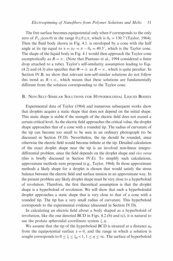
B. NON-SELF-SIMILAR SOLUTIONS FOR HYPERBOLOIDAL LIQUID BODIES

Experimental data of Taylor (1964) and numerous subsequent works show

that droplets acquire a static shape that does not depend on the initial shape.

This static shape is stable if the strength of the electric field does not exceed a

certain critical level. As the electric field approaches the critical value, the droplet

shape approaches that of a cone with a rounded tip. The radius of curvature of

the tip can become too small to be seen in an ordinary photograph (to be

discussed in Section IV.D). Nevertheless, the tip should be rounded, since

otherwise the electric field would become infinite at the tip. Detailed calculation

of the exact droplet shape near the tip is an involved non-linear integro-

differential problem, since the field depends on the droplet shape and vice versa

(this is briefly discussed in Section IV.E). To simplify such calculations,

approximate methods were proposed (e.g., Taylor, 1964). In those approximate

methods a likely shape for a droplet is chosen that would satisfy the stress

balance between the electric field and surface tension in an approximate way. In

the present problem any likely droplet shape must be very close to a hyperboloid

of revolution. Therefore, the first theoretical assumption is that the droplet

shape is a hyperboloid of revolution. We will show that such a hyperboloidal

droplet approaches a static shape that is very close to that of a cone with a

rounded tip. The tip has a very small radius of curvature. This hyperboloid

corresponds to the experimental evidence (discussed in Section IV.D).

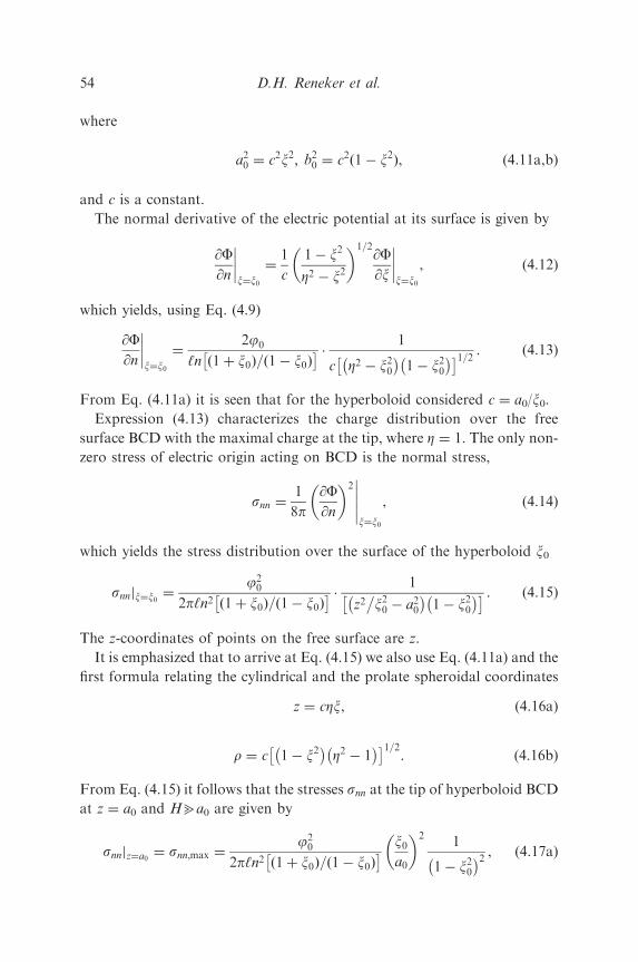
In calculating an electric field about a body shaped as a hyperboloid of

revolution, like the one denoted BCD in Figs. 4.2.(b) and (c), it is natural to

use the prolate spheroidal coordinate system x; Z:We assume that the tip of the hyperboloid BCD is situated at a distance a0

from the equipotential surface z ¼ 0, and the range in which a solution is

sought corresponds to 0 � x � x0o1; 1 � Z � 1: The surface of hyperboloid


BCD is represented by x0 (see Fig. 4.2(c)). Coordinate isolines are also shown

in Fig. 4.2, with the lines Z ¼ const representing ellipsoids, and the lines

x ¼ const representing hyperboloids.

z1 = Hge

z1 = 0

z1See (b)

B D

C0

z

electrode plane

matching boundaryH+a0

ground plane

z1 = Hge

z1

z1 = 0

see (c)

ξ = 0

Bz D

C

ξ = constantξ = ξ0 < 1

η = 1 η = constant

ξ = 00

a0(~100 nm)

ρ

(a)

(b)

(c)

FIG. 4.2. Prolate spheroidal coordinate system about a hyperboloidal liquid body BCD. (a)

Equipotential lines are shown for 0pz1pHge�(H+a0). (c) Equipotential lines (x ¼ const) are

shown for Hge�(H+a0)pz1pHge. After Yarin et al. (2001b) with permission from AIP.


The second theoretical assumption is that the space charge effects are

negligible. This assumption is discussed in detail in Section IV.D. Then the

electric potential F satisfies the Laplace equation. In prolate spheroidal

coordinates it takes the form (Smythe, 1968)

@

@xð1� x2Þ

@F@x

� �þ

@

@ZðZ2 � 1Þ

@F@Z

� �¼ 0, (4.5)

which has the general solution,

F ¼X1m¼0

AmPmðxÞ þ BmQmðxÞ� �

½A0mPmðZÞ þ B0

mQmðZÞ� þ const, (4.6)

where PmðÞ and QmðÞ are Legendre functions and associated Legendre

functions of integer order m, respectively, and Am, Bm, A0m and B0

m are the

constants of integration.

Since in the present case the range of interest includes Z ¼ 1 (cf. Fig. 4.2)

where Qmð1Þ ¼ 1; to have a finite solution we should take B0m ¼ 0: Also in

the present case, it suffices to consider only the first term of Eq. (4.6)

corresponding to m ¼ 0. We then obtain from Eq. (4.6)

F ¼ A000P0ðZÞ½P0ðxÞ þ B00

0Q0ðxÞ� þ const, (4.7)

where, A00

0 ¼ A0A0

0; B00

0 ¼ B0=A0; P0ðZÞ ¼ P0ðxÞ ¼ 1; and Q0ðxÞ ¼ ð1=2Þln½ð1

þxÞ=ð1� xÞ�:Expression (4.7) then takes the form

F ¼ D ‘n1þ x1� x

� �þ const, (4.8)

where D is a constant, determined by the circumstance that the free surface

of the hyperboloid BCD at x ¼ x0 is kept at a potential F0 ¼ j0 þ const:

Then D ¼ j0=‘n ð1þ x0Þ=ð1� x0Þ� �

; and

F ¼ j0

‘n½ð1þ xÞ=ð1� xÞ�‘n½ð1þ x0Þ=ð1� x0Þ�

þ const: (4.9)

Hyperboloid BCD is given by the expression

z2

a20

�r2

b20

¼ 1, (4.10)


where

a20 ¼ c2x2; b2

0 ¼ c2ð1� x2Þ, (4.11a,b)

and c is a constant.

The normal derivative of the electric potential at its surface is given by

@F@n

��x¼x0

¼1

c

1� x2

Z2 � x2

� �1=2@F@x

��x¼x0

, (4.12)

which yields, using Eq. (4.9)

@F@n

��x¼x0

¼2j0

‘n 1þ x0ð Þ= 1� x0ð Þ� � 1

c Z2 � x20�

1� x20� � �1=2 . (4.13)

From Eq. (4.11a) it is seen that for the hyperboloid considered c ¼ a0/x0.Expression (4.13) characterizes the charge distribution over the free

surface BCD with the maximal charge at the tip, where Z ¼ 1. The only non-

zero stress of electric origin acting on BCD is the normal stress,

snn ¼1

8p@F@n

� �2��x¼x0

, (4.14)

which yields the stress distribution over the surface of the hyperboloid x0

snnjx¼x0 ¼j20

2p‘n2 1þ x0ð Þ= 1� x0ð Þ� � 1

z2x20 � a2

0

� 1� x20� � � . (4.15)

The z-coordinates of points on the free surface are z.

It is emphasized that to arrive at Eq. (4.15) we also use Eq. (4.11a) and the

first formula relating the cylindrical and the prolate spheroidal coordinates

z ¼ cZx, (4.16a)

r ¼ c 1� x2�

Z2 � 1� � �1=2

. (4.16b)

From Eq. (4.15) it follows that the stresses snn at the tip of hyperboloid BCD

at z ¼ a0 and Hba0 are given by

snnjz¼a0 ¼ snn;max ¼j20

2p‘n2 1þ x0ð Þ= 1� x0ð Þ� � x0

a0

� �21

1� x20� 2 , (4.17a)


snnjz¼H ¼ snn;min ¼j20

2p‘n2 1þ x0ð Þ= 1� x0ð Þ� � 1

H2x20 � a2

0

� 1� x20� � � .

(4.17b)

It should be noted that the solutions obtained above for the electric field

about hyperboloidal bodies are exact. However, for liquid bodies the shape

of the free surface cannot, a priori, be expected to be a perfect hyperboloid

and should be calculated separately.

Assuming a hyperboloidal shape as an approximation, its curvature is

given by

K ¼b0z=a0

� 2� b2

0 þ b20z

a20

� 2þ b4

0

a20

b0z=a0

� 2� b2

0 þ b20z

a20

� 2h i3=2 . (4.18)

Therefore, the capillary pressure ps ¼ sK at the tip and at a height H

above the tip (see Fig. 4.2) is given by

ps

��z¼a0

¼ s2a0

b20

, (4.19a)

ps

��z¼H

¼ sðb0H=a0Þ

2� b2

0 þ b20H=a2

0

� 2þ b4

0=a20

b0H=a0

� 2� b2

0 þ b20H=a2

0

� 2h i3=2 . (4.19b)

Similar to the first spheroidal approximation used in Taylor (1964), we

approximate the force balance at the hyperboloidal surface by the

expressions

sK jz¼a0 � Dp ¼ snnjz¼a0 , (4.20a)

sK jz¼H � Dp ¼ snnjz¼H . (4.20b)

Assuming that Dp; the difference between the pressure inside and that

outside the surface, is the same at the tip z ¼ a0 and ‘‘bottom’’ z ¼ H; we

obtain

snnjz¼a0 � snnjz¼H ¼ sK jz¼a0 � sK jz¼H . (4.21)

Substituting Eqs. (4.17) and (4.19) into Eq. (4.21), we find the dependence of

j0 on the surface tension coefficient s,


j20

2p‘n2 ð1þ x0Þ=ð1� x0Þ� � x0=a0

1� x20

!2

�1

ðH=a0Þ2� a2

0

� �ð1� x20Þ

24

35

¼ s2a0

b20

�ðb0H=a0Þ

2� b2

0 þ ðb20H=a2

0Þ2þ b4

0=a20

ðb0H=a0Þ2� b2

0 þ ðb20H=a2

0Þ2

� �3=20@

1A. ð4:22Þ

Also from Eq. (4.11) we obtain

b20 ¼ a2

0

1� x20�

x20. (4.23)

Substituting Eq. (4.23) into Eq. (4.22) and rendering Eq. (4.22) dimension-

less, we rearrange it as follows

j20

sa0¼ 2p‘n2 1þ x0

1� x0

� �2x20 �

x0 1� x20� 1=2

H2þ 1

� �=x20 � 2

h i

H=x0� 2

� 1h i3=2

264

375

�x20

1� x20�

1

H=x0� 2

� 1h i

8<:

9=;

�1

. ð4:24Þ

For a given H ¼ H=a0; we obtain from expression (4.24) a dependence of

j20=sa0 on x0 for a stationary liquid body assumed to have a hyperboloidal

shape. In the case of an ‘‘infinite’’ hyperboloid H � 1�

; with its tip at a

distance a0 from the equipotential surface z ¼ 0, expression (4.24) yields

j0 ¼ ðsa0Þ1=2

ð4pÞ1=2‘n1þ x01� x0

� �ð1� x20Þ

1=2, (4.25)

which is analyzed in Section IV.C.

The temptation is to assign the equipotential surface z ¼ 0 to the ground

plate at z1 ¼ 0. This assignment is ruled out, because a0 would then be much

larger than the droplet size. Then the electric field adjoining the droplet

(which is only a small detail of the practically uniform, capacitor-like field

between the electrode and the ground; cf., Fig. 4.2(a)) would be grossly in

error because this calculation does not account for the presence of the

electrode at z1 ¼ Hge: To eliminate this difficulty, we assume that the

equipotential surface z ¼ 0 is situated very close to the droplet tip, at a

distance a0, which is yet to be determined. The electric field between the

matching boundary (cf., Fig. 4.2(b)) and the free surface of the droplet was

already determined, and was described above.


The electric field between the matching boundary and the ground plate at

distances from the tip much larger than a0 is practically unaffected by the

droplet. Thus the electric field in the region between the ground plate and

the matching boundary may be assumed to be that of a parallel-plate

capacitor (cf., Fig. 4.2(a)). The parallel-capacitor field and the field of the

potential F found here in Section IV.B (cf. Fig. 4.2(c)) are to be matched at

z ¼ 0, which enables us to calculate a0 (cf. Fig. 4.2(b)). We can call the space

between the surface z ¼ 0 and the hyperboloid the boundary layer, which is

characterized by the scale a0. The space below z ¼ 0 is then the ‘‘outer field’’

using a fluid-mechanical analogy. It is emphasized that this procedure is

only a crude first approximation, since the normal derivatives of the

potentials (the electric field intensities) are not automatically matched at

z ¼ 0. A much better representation of the field and potential in the

intermediate region could be achieved by matching asymptotic expansions

or computer modeling (cf. Section IV.E). The region where the potential is

not predicted with much precision is shown in gray in Fig. 4.2(b).

We now consider in detail matching of the approximate solutions for the

electric potential. If z1 is the coordinate directed from the ground plate (at

z1 ¼ 0) toward the droplet, then the capacitor-like field is given by

F ¼F0

Hge

z1. (4.26)

Here Hge is the distance between the ground plate and an electrode attached

to the droplet (at potential F0).

Given that the droplet height in the z direction is H, that the borderline

equipotential surface where z ¼ x ¼ 0 is situated at z1 ¼ Hge � H � a0; andmatching the solutions for the potential, we find from Eqs. (4.9) and (4.26)

that the constant in Eq. (4.9) is

const ¼F0

Hge

ðHge � H � a0Þ. (4.27)

Thus, Eqs. (4.9) and (4.27) yield

F ¼ j0

‘n½ð1þ xÞ=ð1� xÞ�‘n½ð1þ x0Þ=ð1� x0Þ�

þ F0ðHge � H � a0Þ

Hge

. (4.28)

For the droplet surface at x ¼ x0, the potential is F ¼ F0 and thus from Eq.

(4.28) we find

j0 ¼F0

Hge

ðH þ a0Þ. (4.29)


Combining Eq. (4.29) with Eq. (4.25), we obtain the equation for a0

ðsa0Þ1=2

ð4pÞ1=2‘n1þ x01� x0

� �1� x20� 1=2

¼F0

Hge

ðH þ a0Þ, (4.30)

which has two solutions. The solution relevant here reads

a0 ¼1

2

1

b2� 2H

� ��

1

4

1

b2� 2H

� �2

� H2

" #1=2, (4.31a)

b ¼F0

Hgeð4psÞ1=2‘n 1þ x0ð Þ=ð1� x0Þ

� �1� x20� 1=2 , (4.31b)

whereas the other one is irrelevant, since it yields a04Hge.

Expression (4.31a) permits calculation of a0 for any given hyperboloidal

droplet (given x0 and H) at any given potential F0. It should be noted that

the results will be accurate if the calculated value of a0 is sufficiently small

relative to H.

C. FAILURE OF THE SELF-SIMILARITY ASSUMPTION FOR HYPERBOLOIDAL

SOLUTIONS

The electric potential between the free surface of a hyperboloidal liquid

body and the equipotential surface z ¼ 0 is given by Eq. (4.9) with j0 as per

Eq. (4.25). To visualize the asymptotic behavior of Eq. (4.9), we should

follow a straight line with a constant slope y, while R tends to infinity (see

Fig. 4.1). Then using Eqs. (4.16a,b) we find

R ¼ ðz2 þ r2Þ1=2 ¼ cðZ2 þ x2 � 1Þ1=2. (4.32)

Also

� tan y ¼rz¼

1� x2�

Z2 � 1� � �1=2Zx

, (4.33)

which yields

Z2 ¼1� x2

1� x= cos y� 2 . (4.34)


Substituting the latter into Eq. (4.32), we find

R ¼ cx

� cos y1� x2

1� ðx= cos yÞ2

" #1=2. (4.35)

It is seen that R ! 1 as x ! � cos y: Then we obtain from Eqs. (4.9) and

(4.25) the potential F as R-N in the following form:

FjR!1 ¼ ðsa0Þ1=2

ð4pÞ1=2 1� x20� 1=2

‘n1� cos y1þ cos y

� �þ const;

p2� y � p,

(4.36)

which shows that the asymptotic value, F, is finite. F does not tend towards

infinity as the self-similarity of Section IV.A implies. Also, in spite of the fact

that Rba0, the dependence on a0 does not disappear from Eq. (4.36) in

contrast with the self-similar behavior of Taylor’s solution given by Eq.

(4.3). Thus, we have an example of a non-self-similar solution with a non-

fading influence of the value of a0, even when Rba0. Details of the shape of

the tip at small distances of the order of a0, affect the solution for F at any R

b a0. In other words, the solution for the field about a hyperboloid depends

on the value of a0 everywhere, while the field surrounding the Taylor cone

does not depend on a0 at Rba0. The field surrounding the hyperboloidal

bodies is always affected by the value of a0, even when R approaches N.

This behavior is quite distinct from that of the boundary-layer theory cases

of jets from a finite orifice and of plumes originating at a finite source, where

the influence of the size of the orifice or source rapidly fades out.

The following observation should be mentioned. In the case of the

parabolic governing equations (the boundary layer theory, Dzhaugashtin

and Yarin, 1977; Schlichting, 1979; Zel’dovich, 1992), or the equation with a

squared parabolic operator (the beam equation describing self-similar

capillary waves, Yarin and Weiss, 1995), self-similar solutions attract the

non-self-similar ones and thus are realizable. On the other hand, in the

present case the governing Laplace equation is elliptic, and its self-similar

solution does not attract the non-self-similar one and therefore could hardly

be expected to be realizable. Moreover, a similar phenomenon was found in

the problem described by the biharmonic (the elliptic operator squared)

equation, namely in the problem on a wedge under a concentrated couple.

The later is known in the elasticity theory as the Sternberg-Koiter paradox

(Sternberg and Koiter, 1958).


The calculated cone, which is tangent to the critical hyperboloid just

before a jet is ejected, is definitely not the Taylor cone. Indeed, in Fig. 4.3 the

dependence of j0=ðsa0Þ1=2 on x0 according to Eq. (4.25) is shown. The

maximal potential at which a stationary shape can exist corresponds to

x0 ¼ 0:834 and j0¼ 4:699ðsa0Þ

1=2: The value x0 corresponds to the critical

hyperboloid. An envelope cone for any hyperboloid can be found using the

derivative

dz

dr

��r!1

¼a0

b0, (4.37)

which follows from Eq. (4.10).

For the critical hyperboloid, using Eq. (4.23), we find

a0

b0¼

x0

1� x20

� �1=2 ¼ 1:51. (4.38)

Therefore, the half angle at the tip of the cone is given by (cf. Fig. 4.1)

a ¼p2� arctan ð1:51Þ, (4.39)

which yields a ¼ 33:5�; which is significantly smaller than the angle for the

Taylor cone aT ¼ 49:3�: Note also that the Taylor cone is asymptotic to a

FIG. 4.3. Dependence of the shape parameter x0 on the electric potential j0 of an infinite

hyperboloid. After Yarin et al. (2001b) with permission from AIP.


hyperboloid possessing a value of x ¼ x0T which should be less than x:Indeed, similar to Eq. (4.38)

a0T

b0T

¼x0T

1� x20T

� 1=2 ¼ tanp2� aT

� �, (4.40)

which yields x0T ¼ cos aT ¼ 0:65: Comparing this value with that for the

critical hyperboloid, x0 ¼ 0:834; we see once more that the critical

hyperboloid is much ‘‘sharper’’ than the one corresponding to the Taylor

cone, since this sharpness increases with x.The left part of the curve with a positive slope in Fig. 4.3 can be realized

pointwise, since there higher potentials correspond to sharper hyperboloids.

By contrast, the right-hand part represents still sharper hyperboloids for

lower potentials, which cannot be reached in usual experiments with a stable

fluid body. The latter means that the right-hand part corresponds to

unstable solutions. It is also emphasized that the critical angle a ¼ 33:5� is

much closer to the experimental values reported in Section IV.D than that of

the Taylor cone.

The results of Sections IV.B and IV.C are equally relevant for inviscid, for

Newtonian or for viscoelastic liquids after the stress has relaxed. All these

manifest in stationary states with zero deviatoric stresses. In the hypothetical

case of a non-relaxing purely elastic liquid or for a viscoelastic liquid with

weak relaxation effects the elastic stresses affect the half-angle value, which

increases (Yarin et al., 2001b).

D. EXPERIMENTAL RESULTS AND COMPARISON WITH THEORY

Two experiments, using sessile and pendant droplets, were performed for

comparison with the theory. In the sessile drop experiment (Fig. 4.4) a

droplet was created at the tip of an inverted pipette by forcing the liquid

through the pipette slowly with a syringe pump. The liquid used was an

aqueous solution of polyethylene oxide (PEO) with a molecular weight of

400,000 and a weight concentration of 6%.

Fluid properties of such solutions including shear and elongational

viscosity, surface tension and conductivity/resistivity are published else-

where (Fong and Reneker, 1999; Reneker et al., 2000; Yarin et al., 2001a).

Their evaporation rate can be described using the standard dependence of

saturation vapor concentration on temperature (Yarin et al., 2001a). For

droplet sizes of the order of 0.1 cm, the evaporation process lasts not less

than 600 s (Yarin et al., 1999). This is much more than the time required to


reach steady state and make measurements (of the order of 1 s). Therefore,

evaporation effects when the photographs were taken are negligible. All the

experiments were done at room temperature. Elevated temperatures were

not studied. Droplet configurations are quite reproducible for a given

capillary size, which was not varied in the present experiments. The effect of

pH was not studied in detail. Addition of sodium chloride to the solution

was discussed in Fong et al. (1999). The electrode material, usually copper,

had no important effect on the ionic conductivity of the solutions (Fong

et al., 1999; Reneker, et al., 2000; Yarin et al., 2001a).

The electric potential was applied between the droplet and a flat metal

collector plate held above the droplet. The droplet was kept at ground

potential for convenience. The potential difference was increased in steps of

about 200V, each step a few seconds long, until a jet formed at the tip of the

droplet. Images of the droplet were made with a video camera. The shape of

the droplet during the step that preceded the formation of the jet was called

the critical shape. Two linear lamps were mounted vertically, behind and on

either side of the droplet. The shape and diameter of the droplet were

demarcated by reflection of the lights, seen as white line on the image

recorded by the video camera. Diffuse back lighting was used for the pendant

drop (Fig. 4.5).

The drops were photographed at a rate of 30 frames s�1. The observed

shape of the droplet is compared with the calculated shape in Fig. 4.6(a).

lamphigh voltage

camera

pump

FIG. 4.4. Sessile drop experiment. After Yarin et al. (2001b) with permission from AIP.


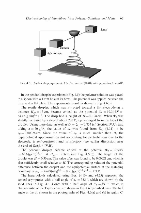
In the pendant droplet experiment (Fig. 4.5) the polymer solution was placed

in a spoon with a 1mm hole in its bowl. The potential was applied between the

drop and a flat plate. The experimental result is shown in Fig. 4.6(b).

The sessile droplet, which was attracted toward a flat electrode at a

distance Hge ¼ 13 cm, became critical at the potential F0 ¼ 19.34 kV ¼

64.47 (g cm)1/2 s�1. The drop had a height of H ¼ 0.128 cm. When F0 was

slightly increased by a step of about 200V, a jet emerged from the top of the

droplet. Using these data, as well as x0 ¼ x0 ¼ 0:834 (cf. Section IV.C), and

taking s ¼ 70 g=s2; the value of a0 was found from Eq. (4.31) to be

a0 ¼ 0.00026 cm. Since the value of a0 is much smaller than H, the

hyperboloidal approximation not accounting for perturbations due to the

electrode, is self-consistent and satisfactory (see earlier discussion near

the end of Section IV.B).

The pendant droplet became critical at the potential F0 ¼ 19.5kV

¼ 65.6 (g cm)1/2s�1 at Hge ¼ 17.3 cm (see Fig. 4.6(b)). The height of the

droplet was H ¼ 0.30 cm. The value of a0 was found to be 0.00021 cm, which is

also sufficiently small relative to H. The corresponding value of the potential

difference between the droplet and the equipotential surface at the matching

boundary is j0 ¼ 4:699ðsa0Þ1=2

¼ 0.57 (g cm)1/2 s�1¼ 171V.

The hyperboloids calculated using Eqs. (4.10) and (4.25) approach the

conical asymptotes with a half angle of a ¼ 33:5�; which are shown by the

solid lines in Fig. 4.6. Cones with a half angle of aT ¼ 49:3�; which is

characteristic of the Taylor cone, are shown in Fig. 4.6 by dashed lines. The half

angle at the tip shown in the photographs of Figs. 4.6(a) and (b) in region C,

lamp

camera

high voltage

FIG. 4.5. Pendant drop experiment. After Yarin et al. (2001b) with permission from AIP.


where the influence of the pipette is small, is 30.51. Even closer to the tip in

region B an observed half angle is 37.51. Both of these angles are closer to the

hyperboloidal solution (33.51) than to the Taylor solution (49.31). Calculation

predicts that the hyperboloid approaches within 5mm of the intersection of the

asymptotes, but there is not enough resolution in the images that this can be

100 µm

A

B

A

B

CC

1mmmm

B

A

B

A

(a) (b)

(d)(c)

FIG. 4.6. (a) Videograph of the critical droplet shape observed for a sessile droplet. The

bottom of the drop was constrained to the inner diameter of the pipette on which it sat. The

drop is symmetrical about the white line. The symmetry axis is not exactly vertical due to

camera tilt, the tilt of the pipette and the tilt of the electric field direction. The half angles

predicted in this section are indicated by the solid lines. The half angle associated with the

Taylor cone is indicated by the dashed lines. This image was not enhanced or cropped. The

outlines of the pipette can be seen at the bottom, and information on the experimental

parameters is visible in the background. (b) Part of the image in (a), processed with Scion image

‘‘find edges’’ (http://www.scioncorp.com/). No useful data about the location of the edge were

found in region A. Lines tangent to the boundary segments in region B indicate a half angle of

37.51. Lines tangent to the boundary segments in region C indicate a half angle of 30.51. The

lower parts of the boundary were not used because they were constrained by the pipette. (c)

Critical droplet shape observed for a pendant drop. (d) Part of the image in (c). The enlarged

droplet tip from (c), processed with Scion image ‘‘find edges.’’ Lines tangent to the boundary

segments in region A indicate a half angle of 311. Lines tangent to the boundary segments in

region B indicate a half angle of 261. After Yarin et al. (2001b) with permission from AIP.


seen. Half angles were measured as shown in Fig. 4.6. For the sessile drop, the

measured half angle near the tip in region B was 37.51 and in region C it was

30.51. For the pendant drop, the measured half angle near the tip in region A

was 311 and in region B was 261. All these angles are closer to the hyperboloidal

solution than to the Taylor cone.

Notice that the electrode used in the experiments was submerged in the

liquid inside the pipette so the influence of the actual electrode on the shape

of the droplet is minimal. The lower part of the droplet shown in Fig. 4.6(a)

is also affected mechanically by the pipette wall, which restricts the diameter

of the base of the droplet. That is the reason why the free surface deviates

from the predicted solid line in Fig. 4.6(a) near the bottom.

According to experimental data, a stable cone can be obtained for a range of

angles, but typically the half angle was close to 45o as stated in Michelson

(1990). Both Taylor (1964) and Michelson (1990) worked with low molecular

weight liquids, which are prone to perturbations and atomization. These

perturbations might lead to premature jetting before a true critical shape can be

achieved. This can explain the larger (and varying) values of a recorded in their

experiments.

In Harris and Basaran (1993), critical configurations of liquid droplets

affected by the electric field in a parallel capacitor were calculated

numerically using the boundary element method. One of the arrangements

considered, the initially hemispherical droplet supported by an electrode, is

close to the experimental situation in the present work. The numerical

predictions for this case (Fig. 42 in Harris and Basaran, 1993) showed that

the apparent cone angle is less than or about 40o, which is closer to the

critical angle a ¼ 33:5� predicted by the above theory than to aT ¼ 49:3�:Wohlhuter and Basaran (1992) using finite-element analysis calculated

steady-state shapes of pendant/sessile droplets in an electric field. Cheng and

Miksis (1989) considered steady-state shapes of droplets on a conducting

plane. Their droplets, however, were considered as polarizable dielectrics

(non-conductors) with no free charges embedded at the free surface. In the

situation characteristic of electrospinning, the fluid behavior corresponds to

that of ionic conductors. Therefore, neither the electric context in the

electrospinning nor the droplet shapes can be related to those predicted in

the above-mentioned works.

The numerically predicted value of the half angle of the calculated shape,

which is significantly less than 49.31, may be an indication of failure of the

self-similarity assumption, similar to what was discussed in Section IV.C.

However, owing to inaccuracies intrinsic in numerical methods in cases in

which a singularity is formed, a definite statement cannot be made.


According to Stone et al. (1999), in which both boundary and finite element

calculations related to the present problem were characterized, ‘‘all the

numerical studies either assume a rounded end and/or cannot resolve the

structure in the neighborhood of a nearly pointed end’’. As usual, close to

singularities, insight can be gained by approximate models, for example, the

slender body approximation (Sherwood, 1991; Li et al., 1994; Stone et al.,

1999), or the hyperboloidal approximation considered above.

It is emphasized that following Taylor (1964), most of the works assume the

liquid in the droplet to be a perfect conductor. In a number of works, however,

cases where liquid in the drop is an insulator, were considered (Li et al., 1994;

Ramos and Castellanos, 1994; Stone et al., 1999). Two self-similar conical

solutions with half angles of 0� � a � 49:3� exist when the ratio of the

dielectric constants is in the range of 17:59 � �d=�s � 1; where ed correspondsto the droplet and es corresponds to a surrounding fluid (the ratio �d=�s ¼ 1

corresponds to the fully conductive droplet). For �d=�so17:59 equilibrium

conical solutions do not exist. Deviation of the experimental half angles to

values significantly below 49.31 can, in principle, be attributed to one of the

two solutions for the range of �d=�s where two solutions exist. The choice

between these solutions based on the stability argument leads to the rather

puzzling outcome that the Taylor cone branch is unstable, and that very small

half angles should be taken in contradiction to experiments (Li et al., 1994;

Stone et al., 1999). However, the assumption that liquids could be considered

as insulators actually holds only on time scales shorter than the charge

relaxation times, tHotC : The latter are of the order of 10�10–10�3 s according

to the estimates of Ramos and Castellanos (1994) and in Section IV.A. Since in

the experiments, the residence time of a liquid in the cone tH is of the order of

1 s and is much longer than the charge relaxation time, conductivity effects

should dominate the dielectric effects (Ramos and Castellanos, 1994). In

insulating dielectric liquids, due to non-zero electric shear stress at the cone

surface, flow is inevitable inside the droplet (Ramos and Castellanos 1994). In

the experiments discussed above such a flow was not seen. The absence of such

a flow is consistent with the fact that the behavior of the polymer solutions

could be closely approximated by that of a perfectly conductive liquid, as was

assumed.

It is of interest to estimate the radius of curvature rc at the tip at the

potential which corresponds to the onset of instability. From Eq. (4.19a), we

have rc ¼ b20=2a0: Using Eq. (4.23) we find

rc ¼ a0

1� x20�

2x20. (4.41)


Substituting x0 ¼ 0.834 and a0 ¼ 0.00026 cm, which are the values found

above, we find rc ¼ 5:69� 10�5 cm; which is near the wavelength of light

and is too small to be seen in an ordinary photograph. Dimensions of

polymer molecules, such as the radius of gyration in the solution, are

typically around 10 nmð10�6 cmÞ; and therefore can be neglected.

In a group of works related to the development of pure liquid alloy ion

sources (LAIS), for example, Driesel et al. (1996) and references therein,

several additional physical processes, which may be relevant within the

context of Taylor cone formation, were revealed. The most important of

them is field evaporation of metal ions from the tip of the cone leading to the

emergence of ion emission currents and space charge. These phenomena are

totally irrelevant in the present context for the following reasons. According

to Driesel et al. (1996) field evaporation is impossible unless a jet-like

protrusion is formed on top of the Taylor cone. The characteristic radius of

curvature of the protruding tip should be of the order of 1–1.5 nm, and the

corresponding field strength of the order of 1.5� 105 kV cm�1. These

conditions could never be realized in the electrospinning experiments. In the

present case, unlike in LAIS, the huge fields needed for field evaporation

could not even be approached. Moreover, the apex temperatures

corresponding to field evaporation and the accompanying effects are of

the order of 600–10001C. Such temperatures would produce drastic chemical

changes in a polymer solution.

In the course of the present work space charge and electrical currents in

the air were occasionally measured. It was shown that the occurrence of

these phenomena was always a consequence of corona discharge, and could

always be reduced to a very low level. All the above taken together allows us

to conclude that field evaporation and ion current effects on the half-angle

of the observed cones can be totally disregarded.

For low-viscosity liquids, as already mentioned, tiny droplets can easily be

emitted from the cone tip. Sometimes droplet emission begins at a close to

451 (Michelson, 1990), sometimes close to 491 (Fernandez de la Mora, 1992).

It should be emphasized that single tiny protrusions, jets and droplets of

submicron size at the top of the Taylor cone are invisible in ordinary

photographs. It is difficult to judge when the jet emerges (cf. Section IV.E)

since the cone tip may oscillate as each droplet separates. At higher voltage,

atomization of the cone tip can lead to significant space charge from the

electrically charged droplets emitted. In Fernandez de la Mora (1992), it was

shown that the backward electric effect of the charged droplets on the tip of

the cone leads to reduction of its half angle to a range of 32�oao46�: Forthe highly viscoelastic liquids used in electrospinning, atomization is


virtually impossible. Breakup of tiny polymer jets, threads and filaments is

always prevented by viscoelastic effects and the huge elongational viscosity

associated with them (Reneker et al., 2000; Stelter et al., 2000; Yarin et al.,

2001a; Yarin, 1993). Therefore, it is highly improbable that the reduced

values of the half angle a� found in the experiments described above can be

attributed to a space charge effect similar to that in Fernandez de la Mora

(1992).

E. TRANSIENT SHAPES AND JET INITIATION

An early attempt (Suvorov and Litvinov, 2000) to simulate numerically

dynamics of Taylor cone formation revealed the following. In one of the two

cases considered, the free surface developed a protrusion, which did not

approach a cone-like shape before the calculations were stopped. In the second

case, a cone-like structure with a half angle of about 50.51 was achieved after

the calculations were started from a very large initial perturbation. It should be

mentioned that the generatrix of the initial perturbation was assumed to be

given by the Gaussian function, and liquid was assumed to be at rest. These

assumptions are arbitrary and non-self-consistent. Also, the assumed initial

shape was far from a spherical droplet relevant within the context of polymeric

fluids. Moreover, the value assumed for the electric field was chosen arbitrarily

and could have exceeded the critical electric field for a stationary Taylor cone.

All these made the results rather inconclusive.

The shape evolution of small droplets attached to a conducting surface

and subjected to relatively strong electric fields was studied both

experimentally and numerically in Reznik et al. (2004) in relation to the

electrospinning of nanofibers. Three different scenarios of droplet shape

evolution were distinguished, based on numerical solution of the Stokes

equations for perfectly conducting droplets. (i) In sufficiently weak

(subcritical) electric fields the droplets are stretched by the electric Maxwell

stresses and acquire steady-state shapes where equilibrium is achieved by

means of the surface tension. (ii) In stronger (supercritical) electrical fields

the Maxwell stresses overcome the surface tension, and jetting is initiated

from the droplet tip if the static (initial) contact angle of the droplet with the

conducting electrode is yso0.8p; in this case the jet base acquires a quasi-

steady, nearly conical shape with vertical semi-angle ap301, which is

significantly smaller than that of the Taylor cone (aT ¼ 49.31). (iii) In

supercritical electric fields acting on droplets with contact angle in the range

0.8poysop there is no jetting and almost the whole droplet jumps off,

similar to the gravity or drop-on-demand dripping. Reznik et al. (2004) used


the boundary integral equations to describe the flow field corresponding to

the axisymmetric creeping flow inside the conducting droplet and the electric

field surrounding it. The equations were solved using the boundary element

method. The parameter representing the relative importance of the electric

and capillary stresses is the electric Bond number, defined as BoE ¼ ‘E21=s;

where ‘ is the characteristic droplet size and EN the applied electric field.

Supercritical scenarios mentioned above correspond to BoE larger than a

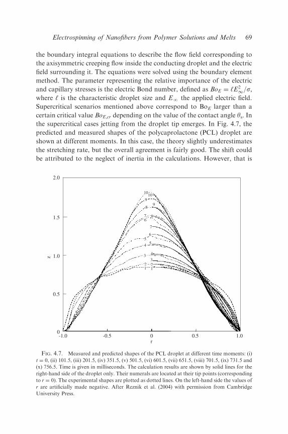
certain critical value BoE;cr depending on the value of the contact angle ys. Inthe supercritical cases jetting from the droplet tip emerges. In Fig. 4.7, the

predicted and measured shapes of the polycaprolactone (PCL) droplet are

shown at different moments. In this case, the theory slightly underestimates

the stretching rate, but the overall agreement is fairly good. The shift could

be attributed to the neglect of inertia in the calculations. However, that is

-1.0 -0.5 0 0.5 1.0r

2.0

0

z

109

8

98

76

7

65

54

43

21

21

10

3

1.5

1.0

0.5

FIG. 4.7. Measured and predicted shapes of the PCL droplet at different time moments: (i)

t ¼ 0, (ii) 101.5, (iii) 201.5, (iv) 351.5, (v) 501.5, (vi) 601.5, (vii) 651.5, (viii) 701.5, (ix) 731.5 and

(x) 756.5. Time is given in milliseconds. The calculation results are shown by solid lines for the

right-hand side of the droplet only. Their numerals are located at their tip points (corresponding

to r ¼ 0). The experimental shapes are plotted as dotted lines. On the left-hand side the values of

r are artificially made negative. After Reznik et al. (2004) with permission from Cambridge

University Press.


not the case: the values of the tip velocity uz measured in the experiments

are: for curve (i) in Fig. 4.7, 0 cm s�1, (ii) 0.058 cm s�1, (iii) 0.110 cm s�1, (iv)

0.142 cm s�1, (v) 0.167 cm s�1, (vi) 0.221 cm s�1, (vii) 0.353 cm s�1, (viii)

0.485 cm s�1, (ix) 0.638 cm s�1 and (x) 0.941 cm s�1; the corresponding values

in the calculations are quite similar. The viscosity of PCL m ¼ 212 P, the

density r ’ 1:32 g cm�3; and the droplet size ‘ ’ 0:1 cm: Therefore, the

highest value of the Reynolds number corresponding to Fig. 4.7 is

Re ¼ 5.86� 10�4 which hardly gives any inertial effects. Experiments on

drop evolution in a high-voltage electric field were also conducted by Zhang

and Basaran (1996). They used low-viscosity fluid (water). The flow

behavior of the droplets in their case was quite distinct from that of the

highly viscous fluids used for electrospinning of nanofibers.

The predicted droplet shapes corresponding to the above-mentioned

scenarios (i) and (ii) are shown in Fig. 4.8; in the present case the critical

value of the electric Bond number BoE,cr is about 3.04.

1.5

1.0

0.5

z

2.0

00

1.5r

i

1.00.5(a) (b)

z

FIG. 4.8. Droplet evolution corresponding to the contact angle ys ¼ p/2; (a) BoE ¼ 3.03:

the subcritical case, curve (i) shows the initial droplet shape at t ¼ 0, the subsequent curves

correspond to the time intervals Dt ¼ 1; (b) BoE ¼ 3.24: the jetting stage emerging in the

supercritical case, (i) t ¼ 12.001, (ii) 12.012, (iii) 12.022, (iv) 12.03, (v) 12.037 and (vi) 12.041.

Time is rendered dimensionless by tH ¼ m‘/s, where m is viscosity. After Reznik et al. (2004)

with permission from Cambridge University Press.


It is emphasized that the average semi-angle a of the cone below the jet base

in Fig. 4.8(b) is approximately 25–301. Reznik et al. (2004) have not been able

to find an approach to the Taylor cone from the subcritical regimes in their

dynamical numerical simulations. The fact that the early supercritical regimes

exhibit jets protruding from the cones with a ¼ 25–301 favors the assumption

that the critical drop configurations (which are very difficult to achieve

numerically) are closer to those predicted by Yarin et al. (2001b) with semi-

vertical angle of 33.51 than to aT ¼ 49.31. The assumption, however, should

be treated with caution, since all the examples considered correspond to

slightly supercritical dynamical cases, where semi-angles a can be smaller

because of the presence of the protrusion. It should be added that Taylor

(1964) and Yarin et al. (2001b) considered infinite liquid bodies: a cone or a

hyperboloid of revolution, respectively. Comparison of these two idealized

models with the experimental or less-idealized numerical situations, where

droplets are finite and attached to a nozzle or a plane surface, should be made

with caution. The base parts of the droplets are mechanically affected by the

nozzle wall, which restricts the diameter of the droplet (Yarin et al., 2001b).

Such a restriction is, however, much less important for a droplet attached to a

plane surface, as in Reznik et al. (2004). On the other hand, near the droplet

tip any effect of mechanical restrictions and the electric stresses resulting from

charge distribution in the areas far from the tip, should be small. That is the

reason why both Taylor cones and hyperboloids could be compared with

experiments and numerical calculations for finite droplets.

Notz and Basaran (1999) carried out a numerical analysis of drop formation

from a tube in an electric field. The flow in the droplets was treated as an

inviscid potential flow. In a subcritical electric field when no jetting is initiated

such a model predicts undamped oscillations of the droplet. Obviously, such

behavior, as well as that in supercritical jetting, is incompatible with the

creeping flow case, characteristic of electrospinning. Experiments with levitated

droplets, also corresponding to the low-viscosity limit, revealed thin jets issuing

from droplet poles and totally disintegrating during 5ms (Duft et al., 2003). This

case is also incompatible with the present one, dominated by the high-viscosity

characteristic of spinnable polymer solutions.

When the critical potential for static cone formation is exceeded and jetting

begins, in the case of polymer solutions the jets are stable to capillary

perturbations, but are subject to bending instability, which is usually observed

in the electrospinning process (see Section V). On the other hand, in the case of

low-viscosity liquids or removal of the charge (Fong et al., 1999), the jets are

subject to capillary instability, which sometimes leads to an almost immediate

disappearance of the jet (Fernandez de la Mora, 1992). Sometimes, however, in


the case of bending or capillary instability a visible, almost straight section of a

jet exists, where the growing perturbations are still very small. Therefore, it is of

interest to describe the jet profile corresponding to the almost straight section.

As noted above, the cone angle in the transient region, where the viscous

inertialess flow transforms into a jet, is ap301. Then, for a description of the

flow in the transient region and in the jet it is natural to use the quasi-one-

dimensional equations, which has been done in a number of works (Cherney,

1999a,b; Feng, 2002, 2003; Ganan-Calvo, 1997a,b, 1999; Hohman et al., 2001a;

Kirichenko et al., 1986; Li et al., 1994; Melcher and Warren, 1971; Stone et al.,

1999) with different degree of elaboration. The solution of these equations

should also be matched to the flow in the drop region. Cherney (1999a,b) used

the method of matched asymptotic expansions to match the jet flow with a

conical semi-infinite meniscus. As a basic approximation for the droplet shape

the Taylor cone of aT ¼ 49.31 was chosen. This choice seems to be rather

questionable in light of finding that the Taylor cone represents a self-similar

solution of the Laplace equation to which non-self-similar solutions do not

necessarily tend even in the case of a semi-infinite meniscus (cf. Sections

IV.A–IV.D). Moreover, even in the situation considered, complete asymptotic

matching has never been achieved. Figs. 2(b), 3 and 4 in Cherney (1999a) depict

discontinuities in the transition region from the meniscus to the jet. Namely, the

solutions for the velocity, the potential and the field strength and the free-

surface configuration are all discontinuous. A similar discontinuity in the

distribution of the free-surface charge density is depicted in Fig. 2 in Cherney

(1999b). In that work it is mentioned that ‘‘rigorous studies of the whole

transition region require significant effort and must be a subject of separate

work’’. The rigorous asymptotic matching is not yet available in the literature,

to the best of our knowledge. Moreover, Higuera (2003) pointed out a formal

inconsistency of Cherney’s (1999a,b) analysis. Approximate approaches were

tested to tackle the difficulty. In particular, Ganan-Calvo (1997a,b, 1999),

Hohman et al. (2001a) and Feng (2002, 2003) extended the quasi-one-

dimensional jet equations through the whole droplet up to its attachment to the

nozzle. Such an approach is quite reasonable, but only as a first approximation,

since the equations are formally invalid in the droplet region, where the flow is

fully two-dimensional. Also, in the electric part of the problem there is a need to

take into account the image effects at the solid wall, which is not always done.

When done, however (e.g. Hohman et al., 2001a), it does not necessarily

improve the accuracy of the results. Fortunately, Feng (2002) showed that all

the electrical prehistory effects are important only in a very thin boundary

layer, adjacent to the cross-section where the initial conditions are imposed

(in his case at the nozzle exit). As a result, there is a temptation to apply the


quasi-one-dimensional jet equations similar to those of Feng (2002) but moving

the jet origin to a cross-section z*40 in the droplet (the value of z* is of the

order of the apparent height of the droplet tip). Based on this idea, Reznik et al.

(2004) matched the flow in the jet region with that in the droplet. By this means,

they predicted the current-voltage characteristic I ¼ I(U) and the volumetric

flow rate Q in electrospun viscous jets, given the potential difference applied.

The predicted dependence I ¼ I(U) is nonlinear due to the convective

mechanism of charge redistribution superimposed on the conductive (ohmic)

one. For U ¼ O(10kV) the fluid conductivity se ¼ 10�4 Sm�1, realistic current

values I ¼ O(102nA) were predicted.

Two-dimensional calculations of the transition zone between the droplet

and the electrically pulled jet at its tip were published in Hayati (1992),

Higuera (2003) and Yan et al. (2003).

F. SUMMARY

The hyperboloidal approximation considered in the present section

permits prediction of the stationary critical shapes of droplets of inviscid,

Newtonian and viscoelastic liquids. It was shown, both theoretically and

experimentally, that as a liquid surface develops a critical shape, its

configuration approaches the shape of a cone with a half angle of 33.5o,

rather than a Taylor cone of 49.3o. The critical half angle does not depend

on fluid properties, since an increase in surface tension is always

accompanied by an increase in the critical electric field.

V. Bending Instability of Electrically Charged Liquid Jets of Polymer

Solutions in Electrospinning

In the present section, the physical mechanism of the electrospinning

process is explained and described following Reneker et al. (2000) and Yarin

et al. (2001a). It is shown that the longitudinal stress caused by the external

electric field acting on the charge carried by the jet stabilizes the straight jet for

some distance. Then a lateral perturbation grows in response to the repulsive

forces between adjacent elements of charge carried by the jet. This is the key

physical element of the electrospinning process responsible for enormously

strong stretching and formation of nanofibers. A localized approximation is

developed to calculate the bending electric force acting on an electrified

polymer jet. Using this force, a far-reaching analogy between the electrically


driven bending instability and the aerodynamically driven instability was

established. Continuous, quasi-one-dimensional, partial differential equations

are derived and used to predict the growth rate of small electrically driven

bending perturbations of a liquid column. A discretized form of these

equations, that accounts for solvent evaporation and polymer solidification, is

used to calculate the jet paths during the course of non-linear bending

instability leading to formation of large loops and resulting in nanofibers. The

results of the calculations are compared to the experimental data. The

mathematical model provides a reasonable representation of the experimental

data, particularly of the jet paths determined from high-speed videographic

observations in set-ups with single and multiple jets.

In Section V.A, the experimental electrospinning single-jet set-up is described.

The experimental observations are presented in Section V.B. In Section V.C, a

model of the rectilinear part of the electrified jet is presented. The basic physics

of bending instability in electrospinning is explained in Section V.D. Localized

approximation for calculation of electrostatic repulsive forces in bending

instability is introduced in Section V.E. Using it, the continuous quasi-one-

dimensional equations of the dynamics of electrified jets are introduced in

Section V.F, and the corresponding discretized equations – in Section V.G.

Solvent evaporation and jet solidification are incorporated in the model in

Section V.H. Growth rate and wavelength of small bending perturbations of an

electrified liquid column are discussed in Section V.I. Non-linear dynamics of

bending and looping in single-jet electrospinning predicted theoretically is

discussed and compared to the experimental data in Section V.J. Section V.K

treats the experimental and theoretical aspects of multiple-jet electrospinning

intended to increase production rate. Conclusions are drawn in Section V.L.

The international system of units (Systeme International (SI)) is used to

report the values of experimental measurements. Gaussian units that are

customary in fluid mechanics and electrostatics have also been used, as well as

dimensionless combinations of parameters to provide concise coverage of the

multi-dimensional parameter space. The numerical results from the calcula-

tions were converted to SI units for comparison with the experimental

observations. Table 5.1 of symbols and Table 5.2 of dimensionless groups of

parameters are provided.

A. EXPERIMENTAL SET-UP FOR ELECTROSPINNING

Fig. 5.1 is a sketch of the experimental apparatus. In this section, words

such as up, down, top and bottom, are used to simplify the description of the


experimental arrangements and the observations. The jet flowed downward

from the surface of a pendant drop of fluid towards a collector at the

distance h below the droplet. An electrical potential difference, which was

around 20 kV, was established between the surface of the liquid drop and the

collector. The distance, h, was around 0.2m. The nanofibers formed a mat

on the collector. The coordinates used in the mathematical description are

also shown. A magnified segment of the jet near the top of the envelope cone

shows the electrical forces that cause the growth of the bending instability.

These forces are described in detail in Section V.D and Fig. 5.27.

In general, the pendant drop may be replaced by other fluid surfaces such

as films on a solid or shapes generated by surface tension and flow. The

collector is usually a good electric conductor. The charged nanofibers may

be collected on an insulator, although a way to neutralize the charge carried

by nanofibers must be provided in order to collect many layers of

nanofibers. Airborne ions from a corona discharge provide an effective

Table 5.1. Symbols employed and their definitions.

Symbol Definition Unit (CGS)

a Cross-sectional radius cm

a0 Initial cross-sectional radius cm

e Charge ðg1=2cm3=2Þ=sfa Air friction force per unit length g=s2

fg Gravity force per unit length g=s2

G Elastic modulus g=ðcm s2Þ

h Distance from pendant drop to grounded collector cm

Lel Length scale, Lel ¼ ðe2=pa20GÞ1=2 cm

Lz Length of the straight segment cm

‘ Length of the ideal rectilinear jet cm

m Mass g

t Time s

v Velocity cm/s

U0 Voltage g1=2cm1=2=sW Absolute value of velocity cm/s

f Initial segment length cm

l Perturbation wavelength cm

m Viscosity g/(cm s)

n Kinematic viscosity cm2=ss Surface tension g=s2

sij Stress g=ðcm s2Þ

r Density g=cm3

ra Air density g=cm3

y Relaxation time ( ¼ m/G) s

o Frequency of the perturbation s�1


way to neutralize the charge on the jets and on the nanofibers. Nanofibers

may also be collected on the surface of a liquid.

Experiments on electrospinning (Reneker and Chun, 1996; Reneker et al.,

2000) typically use set-ups similar to that sketched in Fig. 5.1. All

experiments were performed at room temperature, which was about 201C.

PEO with a molecular weight of 400,000, at a weight concentration of 6%,

was dissolved in a mixture of around 60% water and 40% ethanol. Fresh

solutions produced jets that traveled further before the first bending

instability appears. The solution was held in a glass pipette with an internal

diameter of about 1mm. At the beginning of the experiment, a pendant

droplet of polymer solution was supported at the tip of the capillary. The

liquid jet formed on the surface of the pendant drop of solution.

When the electrical potential difference (measured in volts, and often

referred to as the applied voltage) between the capillary and the grounded

collector is increased, the surface of the liquid becomes charged by the

electrical field-induced migration of ions through the liquid. Instability of

the droplet set in when the potential difference was high enough that

electrical forces overcame the forces associated with surface tension (cf.

Table 5.2. Dimensionless groups and parameters employed and theirdefinitions.

Symbol Dimensionless group Dimensionless

parameter

Definition

A Surface tension ðspa20m2Þ=ðmL2

elG2Þ

H Distance from

pendant drop to

grounded

collector

h=Lel

Ks Perturbation

frequency

om=G

Q Charge ðe2m2Þ=ðL3elmG2Þ

V Voltage ðeU0m2Þ=ðhLelmG2Þ

Fve Elastic modulus ðpa20m

2Þ=ðmLelGÞ

t Time t=ðm=GÞ

W Absolute value of

velocity

W=ðLelG=mÞ

‘ Length of the

rectilinear part of

the jet

‘=Lel

v Velocity v=ðLelG=mÞsij Stress sij=G


Section IV). Above this threshold, a stable liquid jet emerged. The jet carried

away excess ions that migrated to the surface when the potential was

applied. A higher potential difference created a higher charge on the jet. For

low-conductivity solutions, a significant time may be required for the charge

to reach a saturation value after the applied potential changes, since charge

transport within the fluid is limited by the finite mobility of the ions.

A region about 5mm across near the vertex of the envelope cone was

imaged with a lens that had a focal length of 86mm and an f number of 1.0.

The lens was placed about 20 cm from the jet to avoid disturbing the

electrical field near the jet. The image produced by this lens was observed

using a 12.5–75mm, f 1.8 zoom lens on an electronic camera that recorded

upx

yleft

z

pipette

pendantdrop

lamp

fresnel lens

CCD camera

h

force

ne

nanofiberson collector

start of 2nd cycle

front

Conical envelope

FIG. 5.1. Schematic drawing of the electrospinning process, showing the jet path, reference

axes, relative arrangement of parts of the apparatus at different scales and the region where the

bending instability grew rapidly. After Reneker et al. (2000) with permission from AIP.


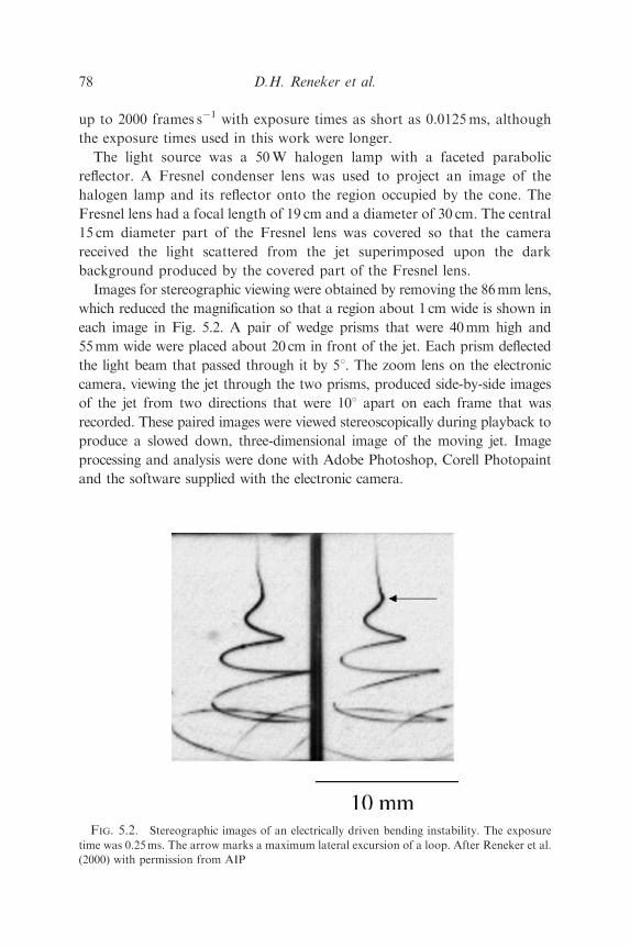
up to 2000 frames s�1 with exposure times as short as 0.0125ms, although

the exposure times used in this work were longer.

The light source was a 50W halogen lamp with a faceted parabolic

reflector. A Fresnel condenser lens was used to project an image of the

halogen lamp and its reflector onto the region occupied by the cone. The

Fresnel lens had a focal length of 19 cm and a diameter of 30 cm. The central

15 cm diameter part of the Fresnel lens was covered so that the camera

received the light scattered from the jet superimposed upon the dark

background produced by the covered part of the Fresnel lens.

Images for stereographic viewing were obtained by removing the 86mm lens,

which reduced the magnification so that a region about 1 cm wide is shown in

each image in Fig. 5.2. A pair of wedge prisms that were 40mm high and

55mm wide were placed about 20 cm in front of the jet. Each prism deflected

the light beam that passed through it by 51. The zoom lens on the electronic

camera, viewing the jet through the two prisms, produced side-by-side images

of the jet from two directions that were 101 apart on each frame that was

recorded. These paired images were viewed stereoscopically during playback to

produce a slowed down, three-dimensional image of the moving jet. Image

processing and analysis were done with Adobe Photoshop, Corell Photopaint

and the software supplied with the electronic camera.

FIG. 5.2. Stereographic images of an electrically driven bending instability. The exposure

time was 0.25ms. The arrow marks a maximum lateral excursion of a loop. After Reneker et al.

(2000) with permission from AIP


B. EXPERIMENTAL OBSERVATIONS

1. Jet Paths

The electrospinning jets typically have an almost straight section of the

order of several centimeters followed by a number of bending loops as

depicted in Fig. 5.1. The straight section will be discussed in more detail in

Section V.B.4. In the present section and in Sections V.B.2 and 3, we discuss

the bending part of the jet. The region near the vertex of the envelope cone

was imaged at 2000 frames s�1. These images showed the time evolution of

the shape of the jet clearly and in detail. Stereographic images such as those

in Fig. 5.2 showed the shape in three dimensions. The expanding spiral in

Fig. 5.2 is a simple example of the kinds of paths that were observed. After a

short sequence of unstable bending back and forth, with growing amplitude,

the jet followed a bending, winding, spiraling and looping path in three

dimensions. The jet in each loop grew longer and thinner as the loop

diameter and circumference increased. Some jets, which are shown in Figs.

5.3–5.5, drifted downward at a velocity much slower than the downward

velocity of the smaller loops close to the vertex of the envelope cone. After

some time, segments of a loop suddenly developed a new bending instability,

FIG. 5.3. Image of the end of the straight segment of the jet. The exposure time was

0.25ms. After Reneker et al. (2000) with permission from AIP.


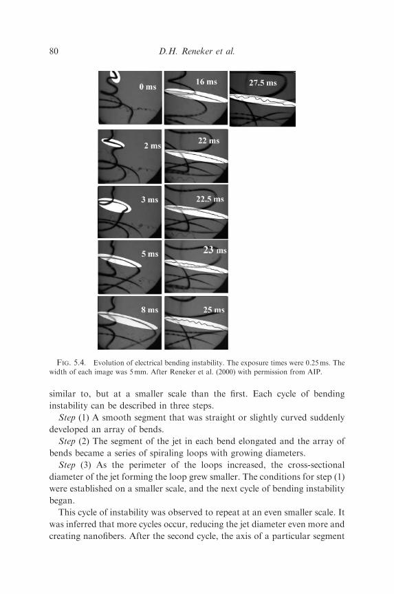
similar to, but at a smaller scale than the first. Each cycle of bending

instability can be described in three steps.

Step (1) A smooth segment that was straight or slightly curved suddenly

developed an array of bends.

Step (2) The segment of the jet in each bend elongated and the array of

bends became a series of spiraling loops with growing diameters.

Step (3) As the perimeter of the loops increased, the cross-sectional

diameter of the jet forming the loop grew smaller. The conditions for step (1)

were established on a smaller scale, and the next cycle of bending instability

began.

This cycle of instability was observed to repeat at an even smaller scale. It

was inferred that more cycles occur, reducing the jet diameter even more and

creating nanofibers. After the second cycle, the axis of a particular segment

FIG. 5.4. Evolution of electrical bending instability. The exposure times were 0.25ms. The

width of each image was 5mm. After Reneker et al. (2000) with permission from AIP.


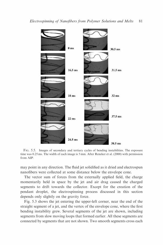
may point in any direction. The fluid jet solidified as it dried and electrospun

nanofibers were collected at some distance below the envelope cone.

The vector sum of forces from the externally applied field, the charge

momentarily held in space by the jet and air drag caused the charged

segments to drift towards the collector. Except for the creation of the

pendant droplet, the electrospinning process discussed in this section

depends only slightly on the gravity force.

Fig. 5.3 shows the jet entering the upper-left corner, near the end of the

straight segment of a jet, and the vertex of the envelope cone, where the first

bending instability grew. Several segments of the jet are shown, including

segments from slow moving loops that formed earlier. All these segments are

connected by segments that are not shown. Two smooth segments cross each

FIG. 5.5. Images of secondary and tertiary cycles of bending instabilities. The exposure

time was 0.25ms. The width of each image is 5mm. After Reneker et al. (2000) with permission

from AIP.


other in this image as they run nearly horizontally across the bottom of the

image. These two segments are noticeably thinner than the jet entering the

image because the jet elongated as time evolved. These slow moving

segments were a part of large loops and were affected both by air drag and

by the disturbance of the applied electrical field caused by the presence of

both charged segments of the jet and charged nanofibers below the region

being observed. Such slow moving segments remained in view for many

frames.

Two thinner segments that formed even earlier are also included in Fig.

5.3. One runs across the top half of the image, and the other runs across the

bottom half. In the lower of these segments, the successive bends (step (1) of

the second cycle) were apparent. In the upper segments, the bends had

already developed into spiraling loops (step (2) of the second cycle). The

pattern of dots visible in the lower left corners of Figs. 5.3–5.5 was caused by

the pattern of facets of the reflector of the halogen lamp used to illuminate

this experiment. These dots are not evidence of the familiar varicose

instability that may cause a liquid jet to become a series of droplets (Yarin,

1993). No varicose instability was observed in this experiment.

Using a set of image files created by the electronic camera it was often

possible to follow the evolution of the shape of spiraling segments, such as

those shown in Fig. 5.3, back to the straight segment that entered the upper-

left-hand corner of the image. In Figs. 5.4 and 5.5, the light ellipse in the first

image marks a segment that evolved in an interesting way. The selected

segment of the jet was followed forward in time, from the moment it entered

the region contained in the images until it elongated, looped, became

unstable, bend, entered the next cycle and ultimately became too thin to

form an image.

Fig. 5.4 starts with a bend near the end of the straight segment of a jet

entering the image at the upper left. The onset of the electrically driven

bending instability occurred just before the jet entered the image. The

straight segment of the jet extended upward, and is not shown. The segment

of the jet that is highlighted by the white ellipse was followed for 27.5ms in a

series of images that were recorded at 0.5ms intervals. The thinner segments

of the jet were emphasized by using the Photopaint 6 software to reproduce

them. Places where the faint image of the jet was ambiguous are indicated by

dots, seen, for example, in the image at 22.5ms.

Eleven images were selected from this series of 55 images to show the

evolution of the highlighted segment. The time intervals between the images

that are shown vary. Many images that show only a gradual evolution of the

path were omitted to simplify Fig. 5.4. The time at which the first image was


captured is taken as time zero. The elapsed time at which each of the

following images was recorded is given in Fig. 5.4.

The looping segment being observed at zero time elongated for 10ms in

Fig. 5.4. Its further elongation was not followed, because the loop had

extended entirely across the image. The rate of increase in the length of the

highlighted segment was around 120mm s�1. After 22ms the visible part of

the highlighted segment still appeared in Fig. 5.4 as a smooth, slightly

curved line. In the short time interval between 22.0 and 22.5ms, this long,

slightly curved smooth segment suddenly became instable. A linear array of

bends appeared, marking the beginning of the second cycle. The lateral

amplitude of the bends grew to about 1mm, and the spatial period of the

bends along the segment was also about 1mm.

These smaller bent segments of the jet continued to elongate, but the

images of the trajectories grew fainter and soon were ambiguous. The

elongation and the associated thinning presumably continued as long as the

charge on the jet supplied enough force. Meanwhile, the elongational

viscosity increased as the jet stretched and dried. Eventually the jet solidified

and the elongation stopped.

The first image in Fig. 5.5 shows a selected segment that was tracked back

to the highlighted area near the bottom of the straight segment. This loop

grew in diameter as the jet elongated and became thinner. After 18ms, an

array of bends that had a relatively long wavelength developed. These bends

evolved gradually to the path shown at 30.5ms. Then a tertiary array of

bends developed on the highlighted segment during the next 0.5ms, and

quickly evolved to the path shown at 31.5ms. The growth of the tertiary

excursions was followed until 38.5ms after the first image, at which point

the jet was so thin that its image could no longer be followed.

2. Jet Splaying/Branching and Garlands

The circled region in Fig. 5.6 shows a jet that split into two jets that

splayed apart, with the axis of the thinner branch generally perpendicular to

the axis of the primary jet (Reneker et al., 2000); cf. with several similar

photographs in Shkadov and Shutov (2001). The thinner jet disappeared in

a few milliseconds, in some cases because it rapidly became even thinner,

and in other cases because its path left the field of view. No bending

instability was observed on the thinner segment, probably because it was not

observed long enough for an instability to develop. Only a few such events

were observed in the thousands of images of PEO solution examined.


Before the high frame rate, short exposure time images of Figs. 5.4 and 5.5

were available, visual observations and video images of electrically driven

PEO solution jets were interpreted as evidence of a process that splayed the

primary jet into many smaller jets. The smaller jets were supposed to emerge

from the region just below the apex of the envelope cone. Fig. 5.7(a) shows

an image from a video frame with an exposure of 16.7ms. The envelope

cone was illuminated with a single bright halogen lamp that projected a

narrow beam through the envelope cone, towards, but not directly into, the

lens, so that most of the light that entered the video camera was scattered

from the jets.

Fig. 5.7(b) shows a jet similar to that shown in Fig. 5.7(a) that was

illuminated with light from two halogen lamps and photographed with a

video camera. The two lamps were above and behind the jet. One was to the

left and the other to the right. This provided a broader source of

illumination than that used for Fig. 5.7(a), but not as uniform as the

FIG. 5.6. A jet splits off the primary jet and splays to a different direction. After Reneker et

al. (2000) with permission from AIP.


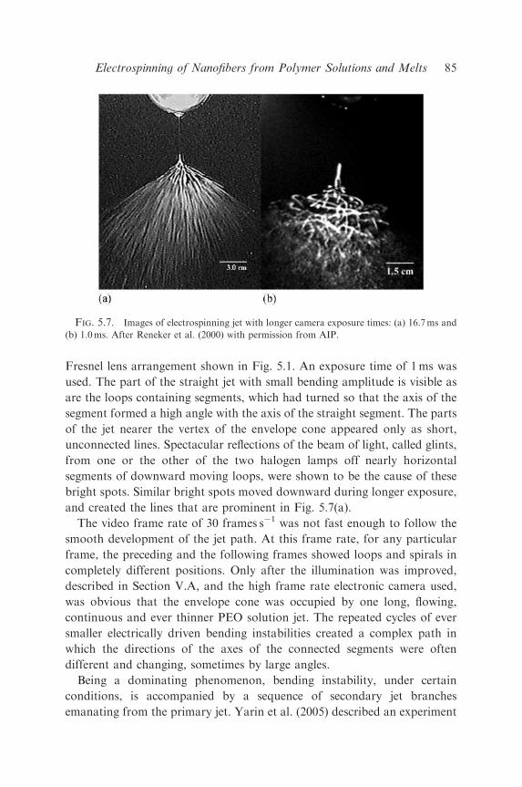
Fresnel lens arrangement shown in Fig. 5.1. An exposure time of 1ms was

used. The part of the straight jet with small bending amplitude is visible as

are the loops containing segments, which had turned so that the axis of the

segment formed a high angle with the axis of the straight segment. The parts

of the jet nearer the vertex of the envelope cone appeared only as short,

unconnected lines. Spectacular reflections of the beam of light, called glints,

from one or the other of the two halogen lamps off nearly horizontal

segments of downward moving loops, were shown to be the cause of these

bright spots. Similar bright spots moved downward during longer exposure,

and created the lines that are prominent in Fig. 5.7(a).

The video frame rate of 30 frames s�1 was not fast enough to follow the

smooth development of the jet path. At this frame rate, for any particular

frame, the preceding and the following frames showed loops and spirals in

completely different positions. Only after the illumination was improved,

described in Section V.A, and the high frame rate electronic camera used,

was obvious that the envelope cone was occupied by one long, flowing,

continuous and ever thinner PEO solution jet. The repeated cycles of ever

smaller electrically driven bending instabilities created a complex path in

which the directions of the axes of the connected segments were often

different and changing, sometimes by large angles.

Being a dominating phenomenon, bending instability, under certain

conditions, is accompanied by a sequence of secondary jet branches

emanating from the primary jet. Yarin et al. (2005) described an experiment

FIG. 5.7. Images of electrospinning jet with longer camera exposure times: (a) 16.7ms and

(b) 1.0ms. After Reneker et al. (2000) with permission from AIP.


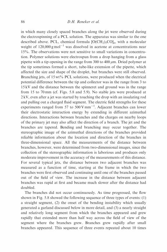
in which many closely spaced branches along the jet were observed during

the electrospinning of a PCL solution. The apparatus was similar to the one

described above. PCL, chemical formula [O(CH2)5CO]n, with a molecular

weight of 120,000 gmol�1 was dissolved in acetone at concentrations near

15%. The observations were not sensitive to small variations in concentra-

tion. Polymer solutions were electrospun from a drop hanging from a glass

pipette with a tip opening in the range from 300 to 400 mm. Dried polymer at

the tip sometimes formed a short, tube-like extension of the pipette, which

affected the size and shape of the droplet, but branches were still observed.

Branching jets, of 15wt% PCL solutions, were produced when the electrical

potential difference between the tip and collector was in the range from 3 to

15 kV and the distance between the spinneret and ground was in the range

from 15 to 70mm (cf. Figs. 5.8 and 5.9). No stable jets were produced at

2 kV, even after a jet was started by touching the drop with an insulating rod

and pulling out a charged fluid segment. The electric field strengths for these

experiments ranged from 57 to 500Vmm�1. Adjacent branches can lower

their electrostatic interaction energy by extending in different azimuthal

directions. Interactions between branches and the charges on nearby loops

of the primary jet may also affect the direction of a branch. The jet and the

branches are tapered. Bending and branching may occur together. The

stereographic image of the azimuthal directions of the branches provided

reliable information about the location and direction of the branches in

three-dimensional space. All the measurements of the distance between

branches, however, were determined from two-dimensional images, since the

collection of the stereographic information is laborious and produces only

moderate improvement in the accuracy of the measurements of this distance.

For several typical jets, the distance between two adjacent branches was

measured as a function of time, starting at the frame in which the two

branches were first observed and continuing until one of the branches passed

out of the field of view. The increase in the distance between adjacent

branches was rapid at first and became much slower after the distance had

doubled.

The branches did not occur continuously. As time progressed, the flow

shown in Fig. 5.8 showed the following sequence of three types of events: (1)

a straight segment, (2) the onset of the bending instability which usually

generated a garland discussed below in more detail, and (3) a nearly straight

and relatively long segment from which the branches appeared and grew

rapidly that extended more than half way across the field of view of the

segment where the branches grew. Branches grew rapidly after small

branches appeared. This sequence of three events repeated about 10 times


per second. The reasons for this repeating sequence are not presently known.

Many such branching events were photographed. Branches were observed

when the dried nanofibers were observed microscopically, but the tangled

paths of the collected nanofibers made it impractical to measure the

relatively long distance between the branches. For a particular branching

event, a frame that showed a number of branches was selected. The spacings

between adjacent branches were determined. Two significant figures were

kept, which are consistent with the precision of the measurement. This

FIG. 5.8. Lateral jets from PCL solution. These ‘‘stopped motion’’ images of a jet were

taken by a high-speed camera at a frame rate of 2000 frame s�1. Every 24th frame is shown here,

so the time separation between the frames shown was about 12ms. The 15% PCL solution was

electrospun at 5 kV, and gap distance from pipette to copper plate collector was 70mm. The

width of each frame is about 14mm. The exposure time of each frame was 0.1ms. Branches are

usually initiated in the straight segment and continue to elongate while the primary jet

undergoes the electrically driven bending instability. The vertical gray line is due to light from

the drop scattered by the camera. This line is not part of the jet. Stereographic images show that

every segment of the primary jet including those segments where a branch is present moved

radially outward and downward as the segment elongated. After Yarin et al. (2005) with

permission from AIP.


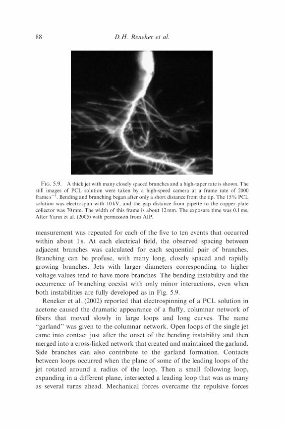
measurement was repeated for each of the five to ten events that occurred

within about 1 s. At each electrical field, the observed spacing between

adjacent branches was calculated for each sequential pair of branches.

Branching can be profuse, with many long, closely spaced and rapidly

growing branches. Jets with larger diameters corresponding to higher

voltage values tend to have more branches. The bending instability and the

occurrence of branching coexist with only minor interactions, even when

both instabilities are fully developed as in Fig. 5.9.

Reneker et al. (2002) reported that electrospinning of a PCL solution in

acetone caused the dramatic appearance of a fluffy, columnar network of

fibers that moved slowly in large loops and long curves. The name

‘‘garland’’ was given to the columnar network. Open loops of the single jet

came into contact just after the onset of the bending instability and then

merged into a cross-linked network that created and maintained the garland.

Side branches can also contribute to the garland formation. Contacts

between loops occurred when the plane of some of the leading loops of the

jet rotated around a radius of the loop. Then a small following loop,

expanding in a different plane, intersected a leading loop that was as many

as several turns ahead. Mechanical forces overcame the repulsive forces

FIG. 5.9. A thick jet with many closely spaced branches and a high-taper rate is shown. The

still images of PCL solution were taken by a high-speed camera at a frame rate of 2000

frame s�1. Bending and branching began after only a short distance from the tip. The 15% PCL

solution was electrospun with 10 kV, and the gap distance from pipette to the copper plate

collector was 70mm. The width of this frame is about 12mm. The exposure time was 0.1ms.

After Yarin et al. (2005) with permission from AIP.


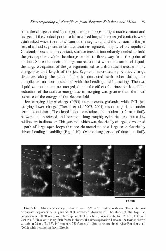
from the charge carried by the jet, the open loops in flight made contact and

merged at the contact point, to form closed loops. The merged contacts were

established when the momentum of the segments and the tension in the jet

forced a fluid segment to contact another segment, in spite of the repulsive

Coulomb forces. Upon contact, surface tension immediately tended to hold

the jets together, while the charge tended to flow away from the point of

contact. Since the electric charge moved almost with the motion of liquid,

the large elongation of the jet segments led to a dramatic decrease in the

charge per unit length of the jet. Segments separated by relatively large

distances along the path of the jet contacted each other during the

complicated motions associated with the bending and branching. The two

liquid sections in contact merged, due to the effect of surface tension, if the

reduction of the surface energy due to merging was greater than the local

increase of the energy of the electric field.

Jets carrying higher charge (PEO) do not create garlands, while PCL jets

carrying lower charge (Theron et al., 2003, 2004) result in garlands under

certain conditions. The closed loops constrained the motion to form a fluffy

network that stretched and became a long roughly cylindrical column a few

millimeters in diameter. This garland, which was electrically charged, developed

a path of large open loops that are characteristic of a large-scale electrically

driven bending instability (Fig. 5.10). Over a long period of time, the fluffy

FIG. 5.10. Motion of a curly garland from a 15% PCL solution is shown. The white lines

demarcate segments of a garland that advanced downward. The slope of the top line

corresponds to 0.58m s�1, and the slope of the lower lines, successively, to 0.7, 1.05, 1.36 and

2.04m s�1. Since only every fifth frame is shown, the time separation between the frames shown

was about 20ms. (7.5 kV, 140mm gap, 250 frames s�1, 2ms exposure time). After Reneker et al.

(2002) with permission from Elsevier.


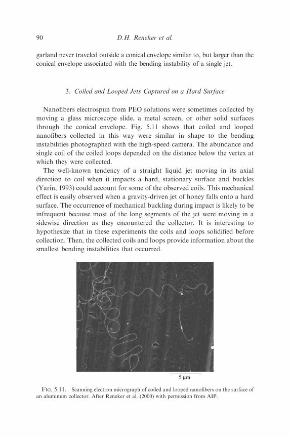
garland never traveled outside a conical envelope similar to, but larger than the

conical envelope associated with the bending instability of a single jet.

3. Coiled and Looped Jets Captured on a Hard Surface

Nanofibers electrospun from PEO solutions were sometimes collected by

moving a glass microscope slide, a metal screen, or other solid surfaces

through the conical envelope. Fig. 5.11 shows that coiled and looped

nanofibers collected in this way were similar in shape to the bending

instabilities photographed with the high-speed camera. The abundance and

single coil of the coiled loops depended on the distance below the vertex at

which they were collected.

The well-known tendency of a straight liquid jet moving in its axial

direction to coil when it impacts a hard, stationary surface and buckles

(Yarin, 1993) could account for some of the observed coils. This mechanical

effect is easily observed when a gravity-driven jet of honey falls onto a hard

surface. The occurrence of mechanical buckling during impact is likely to be

infrequent because most of the long segments of the jet were moving in a

sidewise direction as they encountered the collector. It is interesting to

hypothesize that in these experiments the coils and loops solidified before

collection. Then, the collected coils and loops provide information about the

smallest bending instabilities that occurred.

FIG. 5.11. Scanning electron micrograph of coiled and looped nanofibers on the surface of

an aluminum collector. After Reneker et al. (2000) with permission from AIP.


Cross-sections of the as-spun nanofibers are typically roughly circular.

However, non-circular cross-sectional shapes (presumably due to collapse of

the polymer matrix during solvent evaporation) were also revealed by the

morphological analysis shown by Koombhongse et al. (2001). The collapse

may be so strong that electrospun ribbons appear.

4. Diameter of the Straight Part of the Jet

Xu et al. (2003) developed optical methods for measuring the diameter of

a jet. Diffraction of laser beam is a convenient method for observing the

diameter of the straight segment as a function of position. The tapered shape

of a typical jet is shown in the plot of jet diameter versus distance in

Fig. 5.12. A person can easily monitor the changes in diameter of an

electrospinning jet by observing the position along the path of a distinctive

6

8

10

12

14

16

18

20

-8 -4 0 4 8Distance across the jet

FIG. 5.12. Diameter of the straight segment of a jet as a function of position along the jet.

The graph shows the results of a series of measurements of the diffraction of a laser beam. The

photograph shows the corresponding range of interference colors (Xu, 2003).


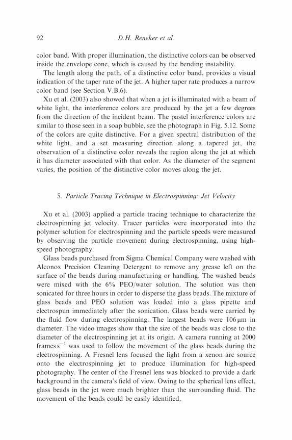
color band. With proper illumination, the distinctive colors can be observed

inside the envelope cone, which is caused by the bending instability.

The length along the path, of a distinctive color band, provides a visual

indication of the taper rate of the jet. A higher taper rate produces a narrow

color band (see Section V.B.6).

Xu et al. (2003) also showed that when a jet is illuminated with a beam of

white light, the interference colors are produced by the jet a few degrees

from the direction of the incident beam. The pastel interference colors are

similar to those seen in a soap bubble, see the photograph in Fig. 5.12. Some

of the colors are quite distinctive. For a given spectral distribution of the

white light, and a set measuring direction along a tapered jet, the

observation of a distinctive color reveals the region along the jet at which

it has diameter associated with that color. As the diameter of the segment

varies, the position of the distinctive color moves along the jet.

5. Particle Tracing Technique in Electrospinning: Jet Velocity

Xu et al. (2003) applied a particle tracing technique to characterize the

electrospinning jet velocity. Tracer particles were incorporated into the

polymer solution for electrospinning and the particle speeds were measured

by observing the particle movement during electrospinning, using high-

speed photography.

Glass beads purchased from Sigma Chemical Company were washed with

Alconox Precision Cleaning Detergent to remove any grease left on the

surface of the beads during manufacturing or handling. The washed beads

were mixed with the 6% PEO/water solution. The solution was then

sonicated for three hours in order to disperse the glass beads. The mixture of

glass beads and PEO solution was loaded into a glass pipette and

electrospun immediately after the sonication. Glass beads were carried by

the fluid flow during electrospinning. The largest beads were 106 mm in

diameter. The video images show that the size of the beads was close to the

diameter of the electrospinning jet at its origin. A camera running at 2000

frames s�1 was used to follow the movement of the glass beads during the

electrospinning. A Fresnel lens focused the light from a xenon arc source

onto the electrospinning jet to produce illumination for high-speed

photography. The center of the Fresnel lens was blocked to provide a dark

background in the camera’s field of view. Owing to the spherical lens effect,

glass beads in the jet were much brighter than the surrounding fluid. The

movement of the beads could be easily identified.


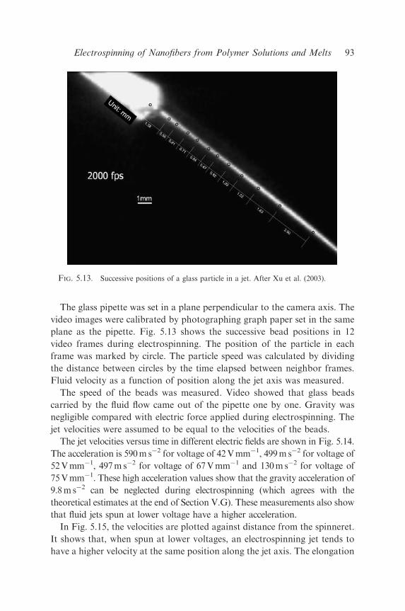
The glass pipette was set in a plane perpendicular to the camera axis. The

video images were calibrated by photographing graph paper set in the same

plane as the pipette. Fig. 5.13 shows the successive bead positions in 12

video frames during electrospinning. The position of the particle in each

frame was marked by circle. The particle speed was calculated by dividing

the distance between circles by the time elapsed between neighbor frames.

Fluid velocity as a function of position along the jet axis was measured.

The speed of the beads was measured. Video showed that glass beads

carried by the fluid flow came out of the pipette one by one. Gravity was

negligible compared with electric force applied during electrospinning. The

jet velocities were assumed to be equal to the velocities of the beads.

The jet velocities versus time in different electric fields are shown in Fig. 5.14.

The acceleration is 590ms�2 for voltage of 42Vmm�1, 499ms�2 for voltage of

52Vmm�1, 497ms�2 for voltage of 67Vmm�1 and 130ms�2 for voltage of

75Vmm�1. These high acceleration values show that the gravity acceleration of

9.8ms�2 can be neglected during electrospinning (which agrees with the

theoretical estimates at the end of Section V.G). These measurements also show

that fluid jets spun at lower voltage have a higher acceleration.

In Fig. 5.15, the velocities are plotted against distance from the spinneret.

It shows that, when spun at lower voltages, an electrospinning jet tends to

have a higher velocity at the same position along the jet axis. The elongation

FIG. 5.13. Successive positions of a glass particle in a jet. After Xu et al. (2003).


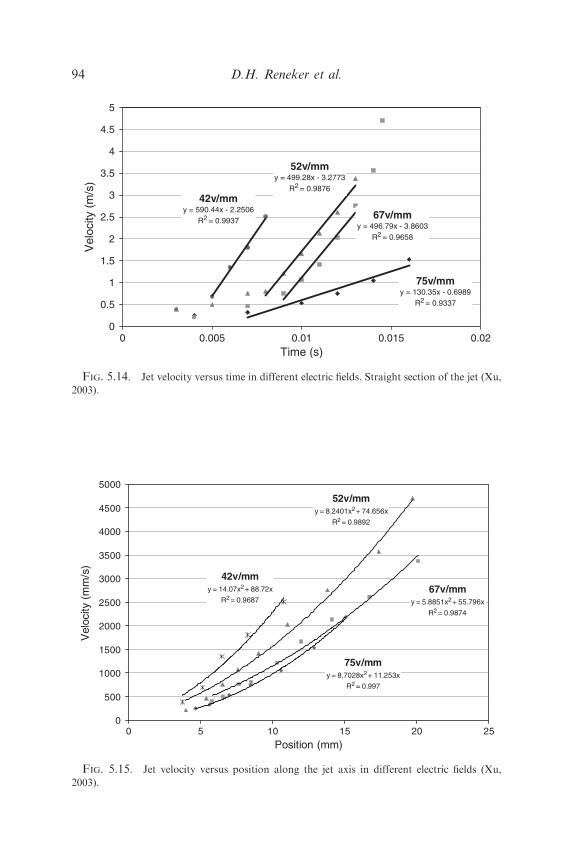
75v/mmy = 130.35x - 0.6989

R2 = 0.9337

67v/mmy = 496.79x - 3.8603

R2 = 0.9658

52v/mmy = 499.28x - 3.2773

R2 = 0.987642v/mm

y = 590.44x - 2.2506R2 = 0.9937

0

0.5

1

1.5

2

2.5

3

3.5

4

4.5

5

0 0.005 0.01 0.015 0.02Time (s)

Vel

ocity

(m

/s)

FIG. 5.14. Jet velocity versus time in different electric fields. Straight section of the jet (Xu,

2003).

75v/mmy = 8.7028x2 + 11.253x

R2 = 0.997

67v/mmy = 5.8851x2 + 55.796x

R2 = 0.9874

52v/mmy = 8.2401x2 + 74.656x

R2 = 0.9892

42v/mmy = 14.07x2 + 88.72x

R2 = 0.9687

0

500

1000

1500

2000

2500

3000

3500

4000

4500

5000

0 5 10 15 20 25

Position (mm)

Vel

ocity

(m

m/s

)

FIG. 5.15. Jet velocity versus position along the jet axis in different electric fields (Xu,

2003).


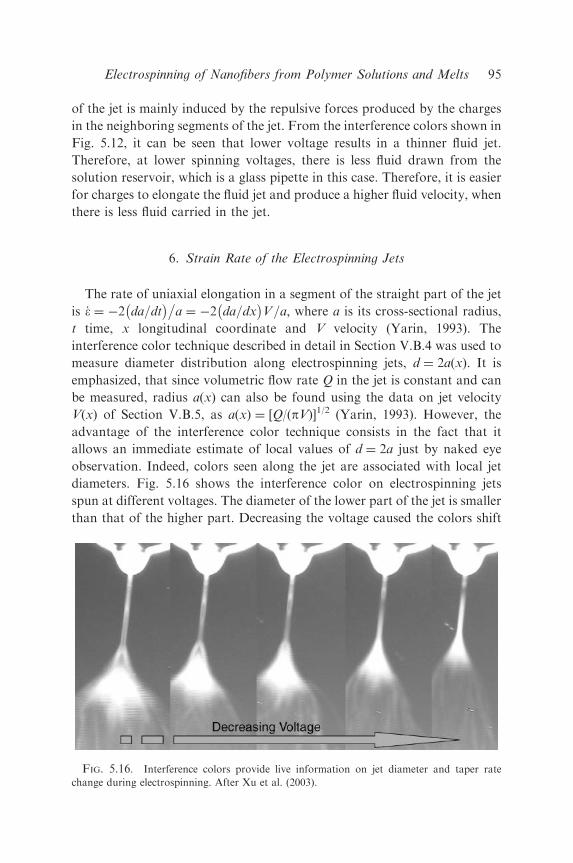
of the jet is mainly induced by the repulsive forces produced by the charges

in the neighboring segments of the jet. From the interference colors shown in

Fig. 5.12, it can be seen that lower voltage results in a thinner fluid jet.

Therefore, at lower spinning voltages, there is less fluid drawn from the

solution reservoir, which is a glass pipette in this case. Therefore, it is easier

for charges to elongate the fluid jet and produce a higher fluid velocity, when

there is less fluid carried in the jet.

6. Strain Rate of the Electrospinning Jets

The rate of uniaxial elongation in a segment of the straight part of the jet

is _� ¼ �2 da=dt�

a ¼ �2 da=dx�

V=a; where a is its cross-sectional radius,

t time, x longitudinal coordinate and V velocity (Yarin, 1993). The

interference color technique described in detail in Section V.B.4 was used to

measure diameter distribution along electrospinning jets, d ¼ 2a(x). It is

emphasized, that since volumetric flow rate Q in the jet is constant and can

be measured, radius a(x) can also be found using the data on jet velocity

V(x) of Section V.B.5, as a(x) ¼ [Q/(pV)]1/2 (Yarin, 1993). However, the

advantage of the interference color technique consists in the fact that it

allows an immediate estimate of local values of d ¼ 2a just by naked eye

observation. Indeed, colors seen along the jet are associated with local jet

diameters. Fig. 5.16 shows the interference color on electrospinning jets

spun at different voltages. The diameter of the lower part of the jet is smaller

than that of the higher part. Decreasing the voltage caused the colors shift

FIG. 5.16. Interference colors provide live information on jet diameter and taper rate

change during electrospinning. After Xu et al. (2003).


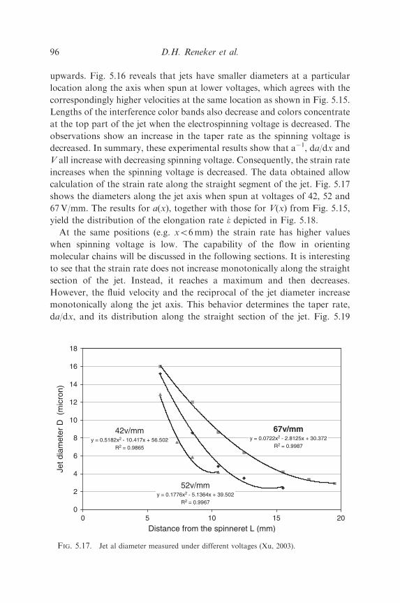
upwards. Fig. 5.16 reveals that jets have smaller diameters at a particular

location along the axis when spun at lower voltages, which agrees with the

correspondingly higher velocities at the same location as shown in Fig. 5.15.

Lengths of the interference color bands also decrease and colors concentrate

at the top part of the jet when the electrospinning voltage is decreased. The

observations show an increase in the taper rate as the spinning voltage is

decreased. In summary, these experimental results show that a�1, da/dx and

V all increase with decreasing spinning voltage. Consequently, the strain rate

increases when the spinning voltage is decreased. The data obtained allow

calculation of the strain rate along the straight segment of the jet. Fig. 5.17

shows the diameters along the jet axis when spun at voltages of 42, 52 and

67V/mm. The results for a(x), together with those for V(x) from Fig. 5.15,

yield the distribution of the elongation rate _� depicted in Fig. 5.18.

At the same positions (e.g. xo6mm) the strain rate has higher values

when spinning voltage is low. The capability of the flow in orienting

molecular chains will be discussed in the following sections. It is interesting

to see that the strain rate does not increase monotonically along the straight

section of the jet. Instead, it reaches a maximum and then decreases.

However, the fluid velocity and the reciprocal of the jet diameter increase

monotonically along the jet axis. This behavior determines the taper rate,

da/dx, and its distribution along the straight section of the jet. Fig. 5.19

52v/mmy = 0.1776x2 - 5.1364x + 39.502

R2 = 0.9967

67v/mmy = 0.0722x2 - 2.8125x + 30.372

R2 = 0.9987

42v/mmy = 0.5182x2 - 10.417x + 56.502

R2 = 0.9865

0

2

4

6

8

10

12

14

16

18

0 5 10 15 20

Distance from the spinneret L (mm)

Jet d

iam

eter

D (

mic

ron)

FIG. 5.17. Jet al diameter measured under different voltages (Xu, 2003).


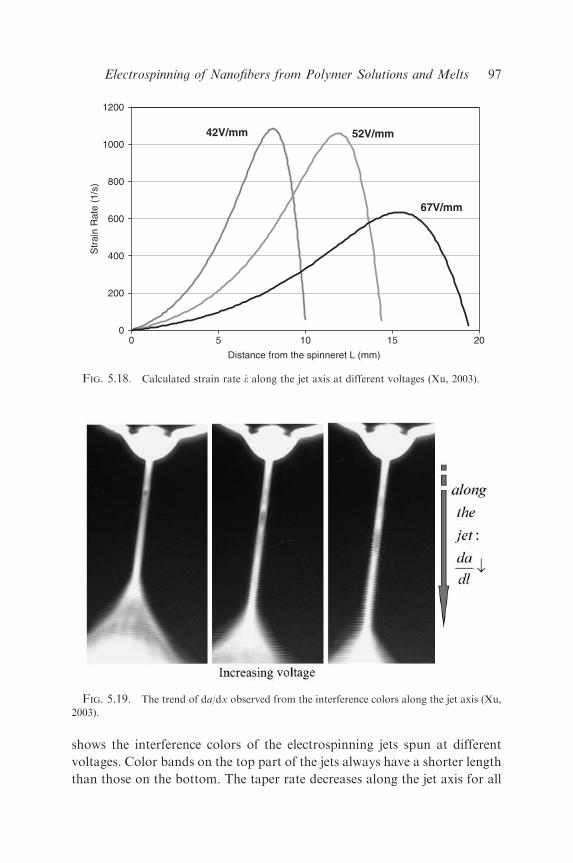
shows the interference colors of the electrospinning jets spun at different

voltages. Color bands on the top part of the jets always have a shorter length

than those on the bottom. The taper rate decreases along the jet axis for all

42V/mm 52V/mm

67V/mm

0

200

400

600

800

1000

1200

0 5 10 15 20

Distance from the spinneret L (mm)

Str

ain

Rat

e (1

/s)

FIG. 5.18. Calculated strain rate _� along the jet axis at different voltages (Xu, 2003).

FIG. 5.19. The trend of da/dx observed from the interference colors along the jet axis (Xu,

2003).


electrospinning voltages. The jet taper rate decreases for the following

reasons: first, a certain degree of molecular chain alignment was achieved

during the early stage of the stretching, making further elongation more

difficult. Second, solvent evaporation caused the elongational viscosity to

increase. Third, the envelope cone below the straight part of the jet is

electrically repulsive, which should decrease tapering. Therefore, when the

decrease of the taper rate exceeds the increase of the fluid velocity and the

reciprocal of the jet diameter, the strain rate starts to decrease.

7. Flow-Induced Molecular Chain Orientation in the Electrospinning Jets

Since the extensional component of the velocity gradient dominates the

shear component in the elongational flow in the electrospinning jets, they

must be very effective in stretching the polymer chains. Polymer chains coil

up in theta or good solvents due to entropy contribution to the free energy.

A strong elongational flow is able to stretch polymer chains resulting in

coil–stretch transition (de Gennes, 1974). In this case, viscous forces exerted

by the flow overbear the entropic elasticity of polymer chains. The strength

of the flow in electrospinning is characterized by the elongational strain rate.

The response of the molecular chains to the flow field depends on the

relaxation time, which characterizes entropic elasticity of macromolecular

chains. The product of the strain rate and the relaxation time determines

whether stretching or relaxation will dominate in the elongation process

(de Gennes, 1974; cf. Section V.J.7). If the flow is weak and molecular chains

are able to return to their original conformation in a short time, the product

of strain rate and relaxation time will be small and relaxation dominates.

Thus, the coiled conformations prevail. If the flow is strong and polymer

chains need a long time to come back to their original conformation, the

product of strain rate and relaxation time will be large. Molecular chains

have no time to rearrange in the flow field. Deformation is stored and added

up. In this case, a coil-stretch transition occurs and the coil quickly reaches a

stretched state.

Fig. 5.20 shows the product of the relaxation time of the polymer solution

and the strain rates of the electrospinning jets spun at different voltages.

PEO/water solutions for this experiment had an initial concentration of 6%.

In Fig. 5.20, the jet spun at the lowest voltages shows the highest value of the

product of strain rate _� and the relaxation time y. Larger value of the

product _�y signify a better molecular chain stretching and alignment by the

flow. It is emphasized that coil-stretch transition is expected for the values of


_�y40.5 (de Gennes, 1974). The latter shows that the three jets of Fig. 5.20

are already strong at their straight sections and should result in stretched

macromolecules. In the next section, birefringence experiment will be used

to investigate the molecular chain alignment under different spinning

voltages.

8. Birefringence of the Electrospinning Jets

From the experimental point of view, the coil-stretch transition has been

studied using birefringence phenomenon. There are some difficulties in

observing the birefringence on electrospinning jets. First, the jet diameter

even at the straight section is only a few microns, which may result in

extremely low birefringence intensity. Second, the liquid in the jet is highly

charged. A certain distance must be maintained, so that the apparatus does

not affect the electric field. To solve the above problems, a set-up as shown

in Fig. 5.21 has been used. In the set-up, light from a 15mW YAG laser

traveled along the z-axis in space. The electric field vector has two

components in the x and y direction. The orientation of the polymer

molecules in the jet will cause the polarizability to become anisotropic. A

sample with oriented molecules should have a different propagation velocity

of light with its electric field vector in the x and the y directions, which

42v/mm 52v/mm

67v/mm

0

10

20

30

40

50

60

0 5 10 15 20 25Distance from the spinneret L (mm)

Str

ain

rate

x r

elax

atio

n tim

e ��

FIG. 5.20. The product of the strain rate and the relaxation time at positions along the

straight section of the jet (Xu, 2003).


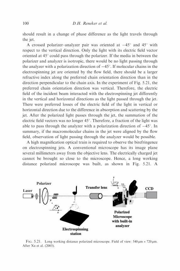
should result in a change of phase difference as the light travels through

the jet.

A crossed polarizer–analyzer pair was oriented at �451 and 451 with

respect to the vertical direction. Only the light with its electric field vector

oriented at 451 could pass through the polarizer. If the media in between the

polarizer and analyzer is isotropic, there would be no light passing through

the analyzer with a polarization direction of �451. If molecular chains in the

electrospinning jet are oriented by the flow field, there should be a larger

refractive index along the preferred chain orientation direction than in the

direction perpendicular to the chain axis. In the experiment of Fig. 5.21, the

preferred chain orientation direction was vertical. Therefore, the electric

field of the incident beam interacted with the electrospinning jet differently

in the vertical and horizontal directions as the light passed through the jet.

There were preferred losses of the electric field of the light in vertical or

horizontal direction due to the difference in absorption and scattering by the

jet. After the polarized light passes through the jet, the summation of the

electric field vectors was no longer 451. Therefore, a fraction of the light was

able to pass through the analyzer with a polarization direction of �451. In

summary, if the macromolecular chains in the jet were aligned by the flow

field, observation of light passing through the analyzer would be possible.

A high magnification optical train is required to observe the birefringence

on electrospinning jets. A conventional microscope has its image plane

several millimeters away from the objective lens. The electrically charged jet

cannot be brought so close to the microscope. Hence, a long working

distance polarized microscope was built, as shown in Fig. 5.21. A

Electrospinningstation

Transfer lens CCD

z

z

Polarized Microscope

with built-in analyzer

Electrospinningstation

Transfer lens CCD

z

zz

Polarized Microscope

with built-in analyzer

Polarizer

Laser z

z

FIG. 5.21. Long working distance polarized microscope. Field of view: 540mm� 720mm.

After Xu et al. (2003).


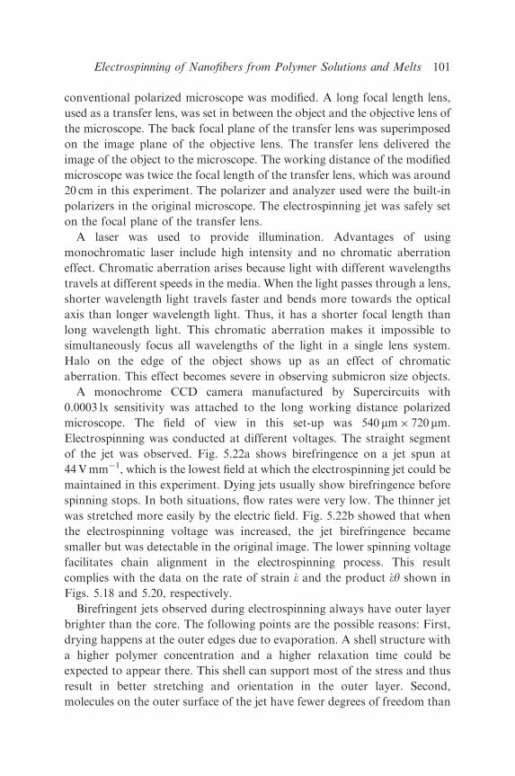
conventional polarized microscope was modified. A long focal length lens,

used as a transfer lens, was set in between the object and the objective lens of

the microscope. The back focal plane of the transfer lens was superimposed

on the image plane of the objective lens. The transfer lens delivered the

image of the object to the microscope. The working distance of the modified

microscope was twice the focal length of the transfer lens, which was around

20 cm in this experiment. The polarizer and analyzer used were the built-in

polarizers in the original microscope. The electrospinning jet was safely set

on the focal plane of the transfer lens.

A laser was used to provide illumination. Advantages of using

monochromatic laser include high intensity and no chromatic aberration

effect. Chromatic aberration arises because light with different wavelengths

travels at different speeds in the media. When the light passes through a lens,

shorter wavelength light travels faster and bends more towards the optical

axis than longer wavelength light. Thus, it has a shorter focal length than

long wavelength light. This chromatic aberration makes it impossible to

simultaneously focus all wavelengths of the light in a single lens system.

Halo on the edge of the object shows up as an effect of chromatic

aberration. This effect becomes severe in observing submicron size objects.

A monochrome CCD camera manufactured by Supercircuits with

0.0003 lx sensitivity was attached to the long working distance polarized

microscope. The field of view in this set-up was 540 mm� 720 mm.

Electrospinning was conducted at different voltages. The straight segment

of the jet was observed. Fig. 5.22a shows birefringence on a jet spun at

44Vmm�1, which is the lowest field at which the electrospinning jet could be

maintained in this experiment. Dying jets usually show birefringence before

spinning stops. In both situations, flow rates were very low. The thinner jet

was stretched more easily by the electric field. Fig. 5.22b showed that when

the electrospinning voltage was increased, the jet birefringence became

smaller but was detectable in the original image. The lower spinning voltage

facilitates chain alignment in the electrospinning process. This result

complies with the data on the rate of strain _� and the product _�y shown in

Figs. 5.18 and 5.20, respectively.

Birefringent jets observed during electrospinning always have outer layer

brighter than the core. The following points are the possible reasons: First,

drying happens at the outer edges due to evaporation. A shell structure with

a higher polymer concentration and a higher relaxation time could be

expected to appear there. This shell can support most of the stress and thus

result in better stretching and orientation in the outer layer. Second,

molecules on the outer surface of the jet have fewer degrees of freedom than


those in the bulk. Chains with less freedom are easier to be aligned by the

flow. Third, like charges always stay away from each other due to the

repulsion forces. Since the electrical relaxation time across the jet is rather

short, essentially all of the charge is concentrated on the surface layer. There

is a higher charge density at the outer surface than in the bulk. Thus,

stronger electrical stretching forces are exerted on the surface layer of the jet.

Fig. 5.23 shows the birefringence of the as-spun fiber obtained under the

same conditions and from the same jet as in Fig. 5.22. Although the fiber

diameter is much smaller than that of the straight section of the jet,

birefringence intensity is a lot stronger. It implies that further chain

alignment took place in the bending loops inside the envelope cone.

The results can be summarized as follows. The ultra-low-intensity

birefringence on the jets during electrospinning was observed. Jets spun at

the very low voltages and the (unstable) dying jets show birefringence. When

increasing the electrospinning voltage, the jet birefringence disappeared.

Birefringence observation complies with the theoretical prediction in Section

V.J.7. Electrospun fibers got under the same condition showed relatively

strong birefringence compared with the straight section of the jet during

electrospinning, which reveals that further chain alignment took place in the

envelope cone area. The strength of the stretching is not the dominant effect

on final fiber diameter. Instead, solidification plays a more important role.

FIG. 5.22. Jet birefringence observed at different electrospinning voltages (Xu, 2003).


Lower electric field produces thinner jets. The large surface area per

unit mass of the thin jet allows solvent to evaporate faster. Hence, thinner

jets experience less time to elongate than thicker ones. Then, the overall

effect makes the electric field effects on the final fiber diameter rather

small.

C. VISCOELASTIC MODEL OF A RECTILINEAR ELECTRIFIED JET

Estimates based on the Maxwell equations, show that all possible

magnetic effects can be safely neglected and the conditions of the

electrohydrodynamics can be assumed.

Consider first a rectilinear electrified liquid jet in an electric field parallel

to its axis. We model a segment of the jet by a viscoelastic dumbbell as

shown in Fig. 5.24. In the mathematical description, we use the Gaussian

electrostatic system of units. Corresponding SI units are given when

parameters are evaluated. Table 5.1 lists the symbols and their units.

Each of the beads, A and B, possesses a charge e and mass m. Let the

position of bead A be fixed by non-Coulomb forces. The Coulomb repulsive

force acting on bead B is �e2/‘2. The force applied to B due to the external

FIG. 5.23. Birefringence on the electrospun fiber (Xu, 2003).


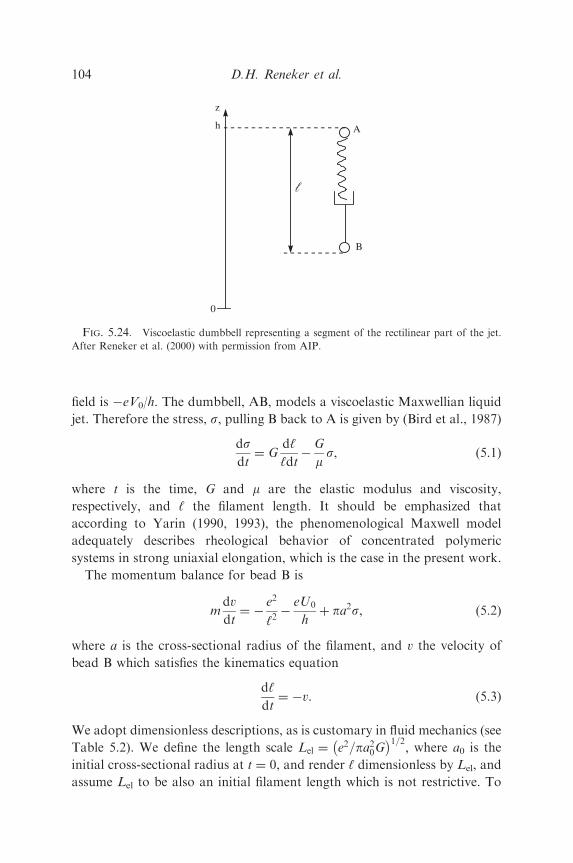
field is �eV0/h. The dumbbell, AB, models a viscoelastic Maxwellian liquid

jet. Therefore the stress, s, pulling B back to A is given by (Bird et al., 1987)

dsdt

¼ Gd‘

‘dt�

G

ms, (5.1)

where t is the time, G and m are the elastic modulus and viscosity,

respectively, and ‘ the filament length. It should be emphasized that

according to Yarin (1990, 1993), the phenomenological Maxwell model

adequately describes rheological behavior of concentrated polymeric

systems in strong uniaxial elongation, which is the case in the present work.

The momentum balance for bead B is

mdv

dt¼ �

e2

‘2�

eU0

hþ pa2s, (5.2)

where a is the cross-sectional radius of the filament, and v the velocity of

bead B which satisfies the kinematics equation

d‘

dt¼ �v. (5.3)

We adopt dimensionless descriptions, as is customary in fluid mechanics (see

Table 5.2). We define the length scale Lel ¼ e2=pa20G

� 1=2; where a0 is the

initial cross-sectional radius at t ¼ 0, and render ‘ dimensionless by Lel, and

assume Lel to be also an initial filament length which is not restrictive. To

A

B

0

h

z

l

FIG. 5.24. Viscoelastic dumbbell representing a segment of the rectilinear part of the jet.

After Reneker et al. (2000) with permission from AIP.


make them dimensionless, we divide t by the relaxation time m/G, stress s by

G, velocity v by LelG=m; and radius a by a0. Denoting W ¼ �v and applying

the condition that the volume of the jet is conserved,

pa2‘ ¼ pa20Lel, (5.4)

we obtain Eqs. (5.1)–(5.3) in the following dimensionless forms:

d‘

dt¼ W , (5.5a)

dW

dt¼ V � Fve

s‘þ

Q

‘2, (5.5b)

dsdt

¼W

‘� s, (5.5c)

where the dimensionless parameters are denoted by bars, and the

dimensionless groups are given by

Q ¼e2m2

L3elmG2

, (5.6a)

V ¼eU0m2

hLelmG2, (5.6b)

F ve ¼pa2

0m2

mLelG. (5.6c)

It is emphasized, that in this momentum balance, we temporarily neglect

the secondary effects of the surface tension, gravity and the air drag force.

Note also that using the definition of Lel, we obtain from Eqs. (5.6a) and

(5.6c) that Q � F ve: It should also be mentioned that here in Eq. (5.4) and

hereinafter in this model, we neglect mass losses due to evaporation. In

principle, they can be accounted for using a specific expression for the

evaporation rate. Evaporation is not expected to introduce qualitative

changes in jet dynamics in the main part of the jet path. However, the effect

of solvent evaporation on the values of the rheological parameters of the

polymer solution ultimately leads to the solidification of the jet into a

polymer fiber. Evaporation and solidification are discussed in detail in

Section V.H.


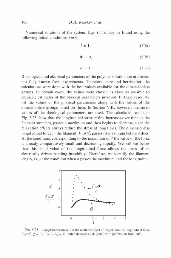
Numerical solutions of the system, Eqs. (5.5), may be found using the

following initial conditions t ¼ 0:

‘ ¼ 1, (5.7a)

W ¼ 0, (5.7b)

s ¼ 0. (5.7c)

Rheological and electrical parameters of the polymer solution are at present

not fully known from experiments. Therefore, here and hereinafter, the

calculations were done with the best values available for the dimensionless

groups. In certain cases, the values were chosen as close as possible to

plausible estimates of the physical parameters involved. In these cases, we

list the values of the physical parameters along with the values of the

dimensionless groups based on them. In Section V.K, however, measured

values of the rheological parameters are used. The calculated results in

Fig. 5.25 show that the longitudinal stress s first increases over time as the

filament stretches, passes a maximum and then begins to decrease, since the

relaxation effects always reduce the stress at long times. The dimensionless

longitudinal force in the filament, Fves=‘; passes its maximum before s does.

At the conditions corresponding to the maximum of s the value of the force

is already comparatively small and decreasing rapidly. We will see below

that this small value of the longitudinal force allows the onset of an

electrically driven bending instability. Therefore, we identify the filament

length, ‘; at the condition when s passes the maximum and the longitudinal

0 1 2 3 4 5

0

1

2

3

4

t

l

F eσv

σl

F eσv

σ

FIG. 5.25. Longitudinal stress s in the rectilinear part of the jet, and the longitudinal force

Fves=‘: Q ¼ 12, V ¼ 2, Fve ¼ 12. After Reneker et al. (2000) with permission from AIP.


force is already small, as the length of the rectilinear segment of the

electrospun jet at which the bending instability begins to grow rapidly. The

relationship of this theoretically defined segment to the observed length of

the straight segment is not yet determined. The length, ‘; increases with

applied voltage as is seen in Fig. 5.26. Near the pendant drop, the

longitudinal force is also small, but the jet does not bend, since its radius

there is large, and the corresponding bending stiffness is large.

The rectilinear liquid jets are unstable to capillary (varicose) perturbations

driven by surface tension. Longitudinal stretching can stabilize the jet in the

presence of these perturbations (Khakhar and Ottino, 1987). In electro-

spinning, jets are stretched along their axis by the external electric field and

are elongated further by the repulsive force between charges on adjacent

segments. The resulting tensile forces prevent development of capillary

instability in the experiments described here.

D. BENDING INSTABILITY OF ELECTRIFIED JETS

Dealing with the bending instability of electrospun jets, we consider the

polymer solutions to be perfect dielectrics with frozen charges. This is

justified by the fact that the bending instability we are going to tackle is

characterized by the characteristic hydrodynamic time, tH ffi 1 ms; and thus

tC4tHðtC ¼ 3:5 ms for se ¼ 10�7 S m�1Þ: Under such conditions the same

fluid, which behaved as a perfect conductor in Taylor’s cone, behaves as a

perfect dielectric in the bending jet. The conductive electric current along the

jet can be neglected, and charge transport can be attributed entirely to the jet

flow (the charge is ‘‘frozen’’ in the liquid).

0 108642 12 14 162

4

6

8

10

12

14

(dim

ensi

onle

ss) l*

V (dimensionless)

FIG. 5.26. Length of the rectilinear part of the jet ‘ as a function of the dimensionless

voltage V. Q ¼ 12 and Fve ¼ 12. After Reneker et al. (2000) with permission from AIP.


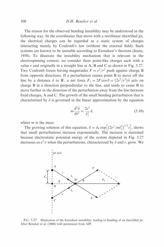
The reason for the observed bending instability may be understood in the

following way. In the coordinates that move with a rectilinear electrified jet,

the electrical charges can be regarded as a static system of charges

interacting mainly by Coulomb’s law (without the external field). Such

systems are known to be unstable according to Earnshaw’s theorem (Jeans,

1958). To illustrate the instability mechanism that is relevant in the

electrospinning context, we consider three point-like charges each with a

value e and originally in a straight line at A, B and C as shown in Fig. 5.27.

Two Coulomb forces having magnitudes F ¼ e2=r2 push against charge B

from opposite directions. If a perturbation causes point B to move off the

line by a distance d to B0, a net force F1 ¼ 2F cos y ¼ 2e2=r3�

d acts on

charge B in a direction perpendicular to the line, and tends to cause B to

move further in the direction of the perturbation away from the line between

fixed charges, A and C. The growth of the small bending perturbation that is

characterized by d is governed in the linear approximation by the equation

md2ddt2

¼2e2

‘21d, (5.10)

where m is the mass.

The growing solution of this equation, d ¼ d0 exp 2e2=m‘31� 1=2

th i

; showsthat small perturbations increase exponentially. The increase is sustained

because electrostatic potential energy of the system depicted in Fig. 5.27

decreases as e2/r when the perturbations, characterized by d and r, grow. We

A

C

B’

r

r

δ θ

F

F

F1

jet axis

l1

B

fl

fl

FIG. 5.27. Illustration of the Earnshaw instability, leading to bending of an electrified jet.

After Reneker et al. (2000) with permission from AIP.


believe that this mechanism is responsible for the observed bending

instability of jets in electrospinning.

If charges A, B and C are attached to a liquid jet, forces associated with

the liquid tend to counteract the instability caused by the Coulomb forces.

For very thin liquid jets, the influence of the shearing force related to the

bending stiffness can be neglected in comparison with the stabilizing effect

of the longitudinal forces since the shearing forces are of the order of O a4�

;

which is much smaller than the longitudinal forces (Yarin, 1993), which are

of the order of O a2�

: The longitudinal force, at the moment when the

bending instability sets in, was calculated above for the stretching of a

rectilinear filament. Its value is given by f ‘ ¼ pa2s (or in dimensionless

form by F ves =‘). The values of s and ‘ at the moment when s (or s)passes its maximum are denoted by asterisks. The forces f‘ are directed along

BC or BA in Fig. 5.27, and are opposite to the local Coulomb force F. If F is

larger than the viscoelastic resistance, f‘, the bending perturbation continues

to grow, but at a rate decelerated by f‘.

It might be thought that bending perturbations of very short lengths can

always overcome the viscoelastic resistance f‘, since the Coulomb force

increases when the wavelength of the perturbation decreases. The surface

tension always counteracts the bending instability because bending always

leads to an increase of the area of the jet surface (Yarin, 1993). Surface

tension resists the development of too large a curvature by the perturbation

ABC in Fig. 5.27, and therefore limits the smallest possible perturbation

wavelengths. All these factors are accounted for in the description of

the three-dimensional bending instability of electrospun jets in Sections V.F

and V.G.

E. LOCALIZED APPROXIMATION

In the dynamics of thin vortices in fluids the localized-induction

approximation is widely used to describe velocity induced at a given vortex

element by the rest of the vortex line (Arms and Hama, 1965; Batchelor,

1967; Aref and Flinchem, 1984; Pozrikidis, 1997; Yarin, 1997). A similar

approach may be used to calculate the electric force imposed on a given

element of an electrified jet by the rest of it. Consider an enlarged element of

a curved jet shown in Fig. 5.28. We assume that the arc length x is reckoned

along the jet axis from the central cross-section of the element where x ¼ 0.

We denote the coordinates reckoned along the normal and binormal by y

and z, so that the position vector of point A on the surface of the element


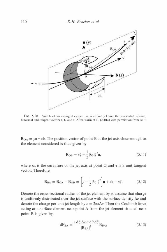
ROA ¼ yn+zb. The position vector of point B at the jet axis close enough to

the element considered is thus given by

ROB ¼ sxþ1

2k0j jx2n, (5.11)

where k0 is the curvature of the jet axis at point O and s is a unit tangent

vector. Therefore

RBA ¼ ROA � ROB ¼ y �1

2k0j jx2

� �nþ zb� sx. (5.12)

Denote the cross-sectional radius of the jet element by a, assume that charge

is uniformly distributed over the jet surface with the surface density De and

denote the charge per unit jet length by e ¼ 2paDe. Then the Coulomb force

acting at a surface element near point A from the jet element situated near

point B is given by

dFBA ¼e dx De a dy dx

RBAj j3RBA, (5.13)

FIG. 5.28. Sketch of an enlarged element of a curved jet and the associated normal,

binormal and tangent vectors n, b, and s. After Yarin et al. (2001a) with permission from AIP.


where y is the polar angle in the jet cross-section. Substituting Eq. (5.12) into

Eq. (5.13) and accounting for the fact that y ¼ a cos y, and z ¼ a sin y we

obtain from Eq. (5.13)

dFBA ¼ e dxDe a dy dxða cos y� jk0jx

2=2Þnþ a sin yb� sx� �a2 � a cos yjk0jx

2þ jk0j

2x4=4þ x2� �3=2 . (5.14)

For a thin jet, as a-0 all the terms containing a in the numerator of Eq.

(5.14) can be safely neglected, also in the denominator the term a cosyjk0jx2

is negligibly small as compared to x2 Then using Eq. (5.14) we calculate the

electric force acting on a particular element of the jet, assuming that the

length of the element is 2L, with L being a cut-off for the integral, to be

determined later on

Fel ¼

Z 2p

0

dyZ L

�L

dFAB ¼ e2dxZ L

�L

dx�sx� jk0jx

2n=2

a2 þ x2 þ jk0j2x4=4

� �3=2 . (5.15)

The latter yields

Fel ¼ e2dxZ L=a

�L=a

dx�sx

að1þ x2Þ3=2

�jk0jx

2n=2

ð1þ x2Þ3=2

" #. (5.16)

The force in the axial direction obviously cancels, whereas the force becomes

Fel ¼ �e2‘nL

a

� �jkjn dx. (5.17)

This shows that the net electric force acting on a jet element is related to its

curvature k ¼ k0, and acts in the normal (lateral) direction to the jet axis.

The magnitude of the net force acting on a jet element due to the action of

the surface tension forces is equal to

F ¼ passjxþdx � passjx ¼ pasjkjn dx, (5.18)

where s is the surface tension coefficient.

Therefore, the net normal (lateral) force acting on a jet element is given by

the sum of the electric and surface tension forces, Eqs. (5.17) and (5.18), as

dF ¼ jkjn dx pas� e2‘nL

a

� �. (5.19)

The cut-off length L is still to be found. It will be done below in Section V.I.


F. CONTINUOUS QUASI-ONE-DIMENSIONAL EQUATIONS OF THE

DYNAMICS OF ELECTRIFIED LIQUID JETS

For very thin jets we can neglect, in the first approximation, the effect of

the shearing force in the jet cross-section, as well as the bending stiffness

(Yarin, 1993, p. 49). If we use a Lagrangian parameter s ‘‘frozen’’ into the jet

elements, then the momentless quasi-one-dimensional equations of the jet

dynamics (Yarin, 1993, p. 49, Eq. (4.19)) take the form

lf ¼ l0f 0, (5.20a)

rl0f 0

@V

@t¼ s

@P

@sþ ljkjPn� rgl0f 0kþ ljkj pas� e2‘n

L

a

� �n� le

U0

hk.

(5.20b)

Equation (5.20a) is the continuity equation with l being the geometrical

stretching ratio, so that lds ¼ dx, and f ¼ pa2 the cross-sectional area.

Subscript zero denotes the parameter values at time t ¼ 0. Equation (5.20b) is

the momentum balance equation with r being the liquid density, V its

velocity, P the longitudinal force in the jet cross-section (of viscoelastic origin

in the case of electrospinning of polymer jets), gk gravity acceleration, U0/h

the outer field strength (the outer field is assumed to be parallel to the unit

vector k, with U0 being the value of electrical potential at the jet origin, and h

the distance between the origin and a ground plate). It is emphasized that on

the right-hand side of the momentum Eq. (5.20b) we account for the

longitudinal internal force of rheological origin acting on the jet (the first two

terms), the gravity force (the third term), the bending electrical force and the

stabilizing effect of the surface tension (the fourth term following from Eq.

(5.19)), and for the electric force acting on the jet from an electric field created

by the potential difference of the starting point of the jet and the collector.

Equations (5.20a,b) are supplemented by the kinematic relation

@R

@t¼ V, (5.21)

where R is the radius vector of a point on the axis of the jet.

Introducing the Cartesian coordinate system associated with a capillary (the

jet origin) or a ground plate, with unit vectors i, j, and k, and accounting for

R ¼ iX þ jY þ kZ, (5.22a)

V ¼ iu þ jv þ kw, (5.22b)


we obtain from the projections of Eqs. (5.20b) and (5.21) the following system

of scalar equations:

rl0f 0

@u

@t¼ tX

@P

@sþ ljkjPnX þ ljkj pas� e2‘n

L

a

� �nX , (5.23a)

rl0f 0

@v

@t¼ tY

@P

@sþ ljkjPnY þ ljkj pas� e2‘n

L

a

� �nY, (5.23b)

rl0f 0

@w

@t¼ tZ

@P

@sþ ljkjPnZ þ ljkj

� pas� e2‘nL

a

� �nZ � rgl0f 0 � le

U0

h, ð5:23cÞ

@X

@t¼ u, (5.23d)

@Y

@t¼ v, (5.23e)

@Z

@t¼ w. (5.23f)

The following geometric relations should be added:

l ¼ X ;2s þ Y ;2s þ Z;2s� 1=2

, (5.24a)

tX ¼1

l@X

@s, (5.24b)

tY ¼1

l@Y

@s, (5.24c)

tZ ¼1

l@Z

@s, (5.24d)

nX ¼1

jkjl@tX

@s, (5.24e)

nY ¼1

jkjl@tY

@s, (5.24f)


nZ ¼1

jkjl@tZ

@s, (5.24g)

jkj ¼X 2

;s þ Y 2;s þ Z2

;s

� �X 2

;ss þ Y 2;ss þ Z2

;ss

� �� X ;sX ;ss þ Y ;sY ;ss þ Z;sZ;ss

� 2X 2

;s þ Y 2;s þ Z2

;s

� �3264

3751=2

ð5:24hÞ

Also assuming the simplest linear version of the upper-convected Maxwell

(UCM) model of viscoelasticity properly fitted to describe uniaxial

elongation (Yarin, 1990, 1993), we obtain the equation for the normal

stress in the jet cross-section stt

@stt@t

¼ G1

l@l@t

�G

mstt, (5.25)

where G is the modulus of elasticity, and m the viscosity, and

1

l@l@t

¼X ;su;s þ Y ;sv;s þ Z;sw;s

l2(5.26)

It is emphasized that any other reliable rheological constitutive equation

could replace Eq. (5.25) in the framework of the present model. In Section

V.K, for example, the non-linear UCM model is used as well, while it is

shown that the difference between the predictions based on the linear and

non-linear UCM models is not large.

The longitudinal force P is given by

P ¼l0f 0

lstt. (5.27)

It is emphasized that in Eq. (5.27) should actually stand the normal stress

stt�snn instead of stt. However, in strong uniaxial elongational flows

(electrospinning is an example of such a flow) the axial component sttbsnn,

and the latter can be neglected. Detailed proof of this fact can be found in

Stelter et al. (2000).

Also the equation of the charge conservation in a jet element holds

el ¼ e0l0 (5.28)

The system of the equations presented in this subsection allows one to find

the jet configuration in space at any moment of time. The equations will be


discretized and solved numerically. It is emphasized that the discretized

equations can also be obtained directly considering the jet to be a locus of

inertial electrically charged beads connected by the spring and dashpot

viscoelastic elements (similar to Section V.D). This is done in the following

subsection.

G. DISCRETIZED THREE-DIMENSIONAL EQUATIONS OF THE DYNAMICS OF

THE ELECTROSPUN JETS

In the present section, we account for the whole integral responsible for

the electric force. This is the only difference with Section V.F where the

bending electric force is calculated using the localized approximation.

We represent the electrospun jets by a model system of beads possessing

charge e and mass m connected by viscoelastic elements as shown in Fig. 5.29,

which generalizes the models of Figs. 5.24 and 5.27. It needs to be mentioned

that these imaginary beads are not the same as the physical beads (Fong et al.,

1999) resulting from the varicose instability. The parameters corresponding to

the element connecting bead i with bead (i+1) are denoted by subscript u

(up), those for the element connecting bead i with (i�1) by subscript d

(down). The lengths ‘ui and ‘di of these elements are given by

‘ui ¼ X iþ1 � X ið Þ2þ Y iþ1 � Y ið Þ

2þ Ziþ1 � Zið Þ

2� �1=2

, (5.29a)

‘di ¼ X i � X i�1ð Þ2þ Y i � Y i�1ð Þ

2þ Zi � Zi�1ð Þ

2� �1=2

, (5.29b)

respectively, where X i;Y i;Zi; . . . ; are the Cartesian coordinates of the beads.

The rates of strain of the elements are given by ðd‘ui=dtÞ=‘ui and

ðd‘di=dtÞ=‘di: The viscoelastic forces acting along the elements are similar to

Eq. (5.1),

dsui

dt¼ G

1

‘ui

d‘ui

dt�

G

msui, (5.30a)

dsdi

dt¼ G

1

‘di

d‘di

dt�

G

msdi. (5.30b)

The total number of beads, N, increases over time as new electrically

charged beads are inserted at the top of Fig. 5.29 to represent the flow of


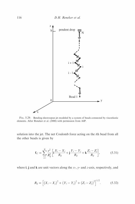
solution into the jet. The net Coulomb force acting on the ith bead from all

the other beads is given by

fC ¼XN

j¼1jai

e2

R2ij

iX i � X j

Rij

þ jY i � Y j

Rij

þ kZi � Zj

Rij

� �, (5.31)

where i, j and k are unit vectors along the x-, y- and z-axis, respectively, and

Rij ¼ X i � X j

� 2þ Y i � Y j

� 2þ Zi � Zj

� 2h i1=2. (5.32)

y

z

ii + 1

i - 1

Bead 1

Npendent drop

x

0

h

FIG. 5.29. Bending electrospun jet modeled by a system of beads connected by viscoelastic

elements. After Reneker et al. (2000) with permission from AIP.


The electric force imposed on the ith bead by the electric field created by the

potential difference between the pendant drop and the collector is

f0 ¼ �eV0

hk. (5.33)

It is clear that the gravitational force may be included in f0.

The net viscoelastic force acting on the ith bead of the jet is

fve ¼ pa2uisui i

X iþ1 � X i

‘ui

þ jY iþ1 � Y i

‘ui

þ kZiþ1 � Zi

‘ui

� �

� pa2disdi i

X i � X i�1

‘di

þ jY i � Y i�1

‘di

þ kZi � Zi�1

‘di

� �, ð5:34Þ

where, when mass is conserved and evaporation neglected, the filament radii

aui and adi are given by

pa2ui‘ui ¼ pa2

0Lel, (5.35a)

pa2di‘di ¼ pa2

0Lel, (5.35b)

which is similar to Eq. (5.4).

The surface tension force acting on the ith bead, and tending to restore the

rectilinear shape of the bending part of the jet, is given by

fcap ¼ �sp a2�

avki

X 2i þ Y 2

i

� 1=2 i X ij jsignðX iÞ þ j Y ij jsignðyiÞ� �

, (5.36)

where s is the surface tension coefficient, ki the jet curvature calculated

using the coordinates of beads (i�1), i and (i+1), and a2�

av¼ ðaui þ

adiÞ2=4: The meaning of ‘‘sign’’ is as follows:

signðxÞ ¼

1; ifx40;

�1; ifxo0;

0; ifx ¼ 0:

8><>: (5.37)

Setting the forces described in Eqs. (5.31), (5.33), (5.34) and (5.36) equal to

mass times acceleration, according to Newton’s second law, we obtain the


equation governing the radius vector of the position of the ith bead

Ri ¼ iX i þ jY i þ kZi in the following form:

md2Ri

dt2¼XN

j¼1jai

e2

R3ij

ðRi � RjÞ � eU0

hkþ

pa2uisui

‘ui

ðRiþ1 � RiÞ

�pa2

disdi

‘di

ðRi � Ri�1Þ �spða2Þavki

ðX 2i þ Y 2

i Þ1=2

½i X ij jsignðX iÞ

þ j Y ij jsignðY iÞ�. ð5:38Þ

For the first bead, i ¼ 1, the total number of beads, N, is also 1. As more

beads are added, N becomes larger and the first bead i ¼ 1 remains at the

bottom end of the growing jet. For this bead, all the parameters with

subscript d should be set equal to zero since there are no beads below i ¼ 1.

Equation (5.38) is essentially a discretized form of Eq. (5.20b) or of its scalar

counterparts, Eqs. (5.23a–f).]

It is easy to show that the aerodynamic drag force and gravity have a

negligibly small effect on the electrospinning. Indeed, for an uncharged jet

moving in air at high speed, an aerodynamically driven bending instability

may set in if raV204s=a; where ra is the air density, V0 the jet velocity, and

s the surface tension coefficient (Entov and Yarin, 1984; Yarin, 1993).

Taking, for example, ra ¼ 1:21 kg m�3; V 0 � 0:5 m s�1; s � 0:1 kg s�2 and

a � 10�4 m; we estimate raV20 � 0:3 kg m s�2; which is much smaller than

s=a � 103 kg m s�2: Therefore, under the conditions characteristic of the

experiments on electrospinning, the aerodynamically driven bending

instability does not occur.

The air drag force per unit jet length, which tends to compress the jet

along its axis, is given by (Ziabicki and Kawai, 1985)

f a ¼ paraV 200:65

2V0a

na

� ��0:81

, (5.39)

where na is the air kinematic viscosity. The gravity force per unit length

pulling the jet downward in the experimental geometry shown in Fig. 5.1 is

f g ¼ rgpa2, (5.40)

where r is the liquid density and g the acceleration due to gravity.

In the momentum balance, Eqs. (5.2) or (5.5b), we neglected fg as a

secondary effect. The air drag force fa is even smaller than fg. Taking ra ¼1:21 kg m�3; na ¼ 0:15� 10�4 m2 s�1; r ¼ 1000 kg=m2;V0 ¼ 0:5 m s�1 and

a ¼ 150mm we obtain from Eqs. (5.39) and (5.40) f a ¼ 1:4� 10�5kg=s2 and


f g ¼ 6:9� 10�4kg=s2: The compressive stress along the jet axis of the air

drag is negligibly small in comparison with the stretching due to gravity, and

is much smaller than the stretching due to the electrical forces. Buckling of

the electrospun jet due to the compressive force from air drag does not

occur, since the electrical forces that tend to elongate the jet are larger and

dominate any perturbation that might lead to buckling.

H. EVAPORATION AND SOLIDIFICATION

The systems of governing equations in Sections V.F and V.G do not

account for the evaporation and solidification effects. We account for them

in the present subsection.

In Ziabicki (1976), the following correlation is given for the Nusselt

number for a cylinder moving parallel to its axis in air

Nu ¼ 0:42 Re1=3, (5.41)

where the Reynolds number Re ¼ V02a=na; a is the cross-sectional radius,

and na the kinematic viscosity of air.

Taking the Prandtl number of air to be Pr ¼ 0.72, we can generalize

correlation (5.41) for an arbitrary value of the Prandtl number as

Nu ¼ 0:495Re1=3 Pr1=2. (5.42)

Similarly, to (5.42), we take the following correlation for the Sherwood

number

Sh ¼ 0:495Re1=3 Sc1=2, (5.43)

where Sh ¼ hm2a/Da, hm is the mass transfer coefficient for evaporation, Da

the vapor diffusion coefficient in air, and the Schmidt number Sc ¼ na/Da.

The Sherwood number is the dimensionless mass transfer coefficient

describing the evaporation rate.

Correlations of the type of Eqs. (5.41)–(5.43) are valid for air (Pr ¼ 0.72) for

Reynolds number in the range 1 � Re � 60: For a � 10�2 cm;V0 � 102 �

103 cm s�1 and na ¼ 0:15 cm2 s�1; the Reynolds number is 10 � Re � 102

which corresponds approximately to the range of validity.

The initial mass of polymer in a jet element is given by

Mp0 ¼ rf 0l0 ds cp0, (5.44)


where cp0 is the initial polymer mass fraction. The variable solvent content

in the element is

Ms ¼ rf l ds � rf 0l0 ds cp0 (5.45)

which corresponds to the solvent mass fraction

cs ¼ 1�f 0l0f l

cp0. (5.46)

The solvent mass decreases due to evaporation according to the equation

@Ms

@t¼ �rhm cs;eqðTÞ � cs1

� �2pal ds, (5.47)

where cs,eq (T) is the saturation vapor concentration of solvent at

temperature T, and cs1 the vapor concentration in atmosphere far from

the jet.

For water as a solvent, for example, Seaver et al. (1989) recommend the

following expression for cs,eq (T):

cs;eq ¼1

1013a0 þ T a1 þ T a2 þ Tða3 þ Tða4 þ Tða5 þ a6TÞð ÞÞÞ½ � �

, (5.48)

a0 ¼ 6.107799961,

a1 ¼ 4.436518521� 10�1,

a2 ¼ 1.428945805� 10�2,

a3 ¼ 2.650648731� 10�4,

a4 ¼ 3.031240396� 10�6,

a5 ¼ 2.034080948� 10�8,

a6 ¼ 6.136820929� 10�11,

where T is taken in degrees Celsius.

Concentration csN is equal to a relative humidity in the atmosphere.

Substituting Eqs. (5.43) and (5.45) into Eq. (5.47), we obtain the equation

describing the variation of the jet volume

@f l@t

¼ �Da 0:495 Re1=3Sc1=2 cs;eqðTÞ � cs1� �

pl. (5.49)


Solvent mass decreases until the solvent mass ratio defined by Eq. (5.47)

becomes small enough (say, cs ¼ 0.1), at which point the evaporation part

of the calculation is stopped and viscosity remains a constant value. This

cut-off can be rationalized by the assumption that further evaporation is

reduced because the diffusion coefficient of solvent in the remaining polymer

is small.

When evaporation is accounted for as per Eq. (5.49), the left-hand sides of

Eqs. (5.20b), and (5.23a)–(5.23c) become, respectively

r@f lV@t

, (5.50a)

r@f lu

@t, (5.50b)

r@f lv

@t, (5.50c)

r@f lw

@t. (5.50d)

Also the gravity term in Eq. (5.23c) should contain fl instead of f0l0, sincedue to evaporation fl is not equal to f0l0 any more.

If the discretized version of the model described in Section V.G is used, lin Eq. (5.49) is replaced by the distance between two adjoining beads.

The local polymer mass ratio in the jet is given by

cp ¼ cp0f 0l0f l

. (5.51)

We account for the solidification process due to solvent evaporation

employing the following correlation for the viscosity dependence on

polymer concentration (Ziabicki, 1976)

m ¼ 10A � 10Bcmp , (5.52)

with m ¼ 0.1 to 1.

The value of parameter B is estimated as follows. According to Ziabicki

(1976, p. 32), when cp is doubled, viscosity of the solution increases by a

factor of 10–102. Using the value 102 and assuming that cp increased from

0.1 to 0.2, we find for m ¼ 1 that B ¼ 20. The value of B ¼ 17.54

corresponds to the factor of 10 and m ¼ 0.1. Therefore the order of

magnitude estimate of B yields the value B ¼ O(10). The value of A is

unimportant, since the initial value of the viscosity m0 ¼ 10A � 10Bcmp0 is


assumed to be known and is used for scaling. On the other hand, the

relaxation time y is proportional to cp (Yarin, 1993). Therefore

yy0

¼cp

cp0, (5.53)

where the initial relaxation time in known.

The modulus of elasticity G ¼ m/y. Rendering the equations of the

problem dimensionless, we obtain the rheological constitutive Eq. (5.25) in

the following dimensionless form:

@stt@t

¼ G@ll@t

�G

mstt. (5.54)

Here G is rendered dimensionless by G0 ¼ m0=y0; and m by m0: There-fore,

G ¼10B cm

p �cmp0

� cp

cp0

, (5.55)

m ¼ 10B cmp �cm

p0

� , (5.56)

with B ¼ O(10).

I. GROWTH RATE AND WAVELENGTH OF SMALL BENDING

PERTURBATIONS OF AN ELECTRIFIED LIQUID COLUMN

In the works of Yarin (1993) and Entov and Yarin (1984), the theory of

the aerodynamically driven jet bending was described. In that case, due to

the jet curvature, a distributed lift force acts on the jet (because of the

Bernoulli equation for airflow), which enhances perturbations and makes

the perturbations grow. The aerodynamic bending force per jet length dx in

the case of small bending perturbations is given by (Entov and Yarin, 1984;

Yarin, 1993)

Faer ¼ �raV20pa2

0 kj j ndx, (5.57)

where ra is the air density, V0 the jet velocity and a0 the jet cross-sectional

radius which does not change for small perturbations.

This force is the only difference between the aerodynamic- and electric-

driven bending. Comparing Eq. (5.17) (with e ¼ e0) with Eq. (5.57), we see

that all the results obtained in the above-mentioned references for the

aerodynamic bending may also be used here in the case of electric bending, if


one replaces the factor raV20 by e20‘nðL=a0Þ=pa2

0: Dynamics of small bending

perturbations was studied in the above-mentioned references accounting for

the shearing force and moment in jet cross-section (thus, accounting for the

bending stiffness in the equations generalizing Eq. (5.23)). For example, the

case of viscous Newtonian fluid was considered. We recast these results here

for the case of an electrified-liquid column of Newtonian fluid of viscosity m.In particular, this generalizes the results of Taylor (1969) to the viscous case,

and allows us to find the cut-off length L.

Recasting the results of Yarin (1993) and Entov and Yarin (1984), we find

that the destabilizing electric force overcomes the stabilizing effect of the

surface tension if

e20‘nL

a0

� �4pa0s. (5.58)

If we assume a0 ¼ 0.015 cm, and the jet charge of 1CL�1, then

e0 ¼ 2120.5 (g cm)1/2 s�1. Below, we show that a reasonable value of L is

L ¼ 0.0325 cm. Using it for the estimate, we find that e20‘nðL=a0Þ ¼ 3:465�

106 g cm s�2; whereas pa0s ¼ 3:3 g cm s�2 for s ¼ 70 g s�1: Therefore, in

this case the inequality (5.58) definitely holds and the bending instability

should set in and grow.

From the results of Yarin (1993) and Entov and Yarin (1984), we obtain

in the present case that the wavenumber wn and the growth rate gn of the

fastest growing bending perturbation are given by

wn ¼8

9

ra20

m2e20‘nðL=a0Þ

pa20

�sa0

� �� 1=6

, (5.59a)

gn ¼e20‘nðL=a0Þ=pa2

0 � s� �2=3

ð3mra40Þ

1=3. (5.59b)

Here wn ¼ 2pa0=‘n; where ‘ is the wavelength of the fastest growing

perturbation.

Results (5.59) correspond to the maximum of the spectrum gðwÞ given by

the characteristic equation

g2 þ3

4

mw4

ra20

gþsra3

0

�e20‘nðL=a0Þ

pra40

� �w2 ¼ 0. (5.60)

This equation is to be compared with the characteristic equation for

electrically driven bending perturbations of an inviscid liquid (m ¼ 0)

column derived by Taylor (1969, his Eq. (12)). Expanding that equation in


the long-wave limit as the dimensionless wavenumber w ! 0; we find that it

reduces to Eq. (5.60) with the term ‘n 1=wn�

instead of ‘nðL=a0Þ: This fact

defines the cut-off length L, since the result of Taylor (1969) is exact. Thus,

taking ‘nðL=a0Þ ¼ ‘nð1=wnÞ and neglecting the minor surface tension effect

in Eq. (5.59a), we reduce the latter to the form

wn ¼8

9

rm2

e20p‘n

1

wn

� �� 1=6, (5.61)

which is the equation defining wn (and thus, L). Taking the same values of

the parameters as before, as well as r ¼ 1 g cm�3 and m ¼ 104 g cm sð Þ�1

(remember that e0 ¼ 2120.5 (g cm)1/2 s�1), we reduce Eq. (5.61) to the form

w ¼ 0:483 ‘n1

w

� �� 1=6(5.62)

which yields wn ¼ 0:462:

Therefore, the wavelength of the fastest growing perturbation ‘ ¼2p 0:015=0:462 ¼ 0:204 cm; and the cut-off length L ¼ ‘=2p ¼ 0:0325 cm:

Comparing the latter with the jet cross-sectional radius a0 ¼ 0.015 cm, we

see that the cut-off length is very short, of the order of a0.

Based on the results of Yarin (1993) and Entov and Yarin (1984), it also

follows that the bending perturbations of highly viscous liquids grow much

faster than the capillary ones (driven by the surface tension), if the condition

pm2

re20‘nðL=a0Þ� 1 (5.63)

is fulfilled. For the values of the parameters used in the present subsection,

the left-hand side of Eq. (5.63) is equal to 90.7, which shows that inequality

(5.63), indeed, holds. Therefore, such a jet bends with a nearly constant

radius.

J. NON-LINEAR DYNAMICS OF BENDING ELECTROSPUN JETS

To model the way a spatial perturbation develops, we denote the last bead

pulled out of the pendant drop and added at the upper end of the jet by

i ¼ N. When the distance ‘d,N between this bead and the pendant drop

becomes long enough, say, h/25,000, a new bead i ¼ N+1 is inserted at a


small distance, say, h/50,000, from the previous one. At the same time a

small perturbation is added to its x and y coordinates,

X i ¼ 10�3Lel sinðotÞ, (5.64a)

Y i ¼ 10�3Lel cosðotÞ. (5.64b)

Here, o is the perturbation frequency. The condition that the collector at

z ¼ 0 is impenetrable is enforced numerically, and the charge on each

element of the jet is removed as it arrives at the collector. Such a calculation

mimics the development of the electrically driven bending instability. The

calculation begins with only two beads, N ¼ 2. As the jet flows, the number

of beads in the jet, N, increases. In the cases when evaporation and

solidification were not accounted for, the system of Eqs. (5.30) and (5.38)

was solved numerically, assuming that the stresses sui and sdi, and the

velocity dRi/dt were zero at t ¼ 0. The equations were made dimensionless

by the same scale factors as those in Section V.C. Since here it is necessary to

account for the surface tension and for the perturbing displacements, two

new dimensionless groups emerge in addition to those of Eqs. (5.6)

A ¼spa2

0m2

mL2elG

2, (5.65a)

Ks ¼ om=G. (5.65b)

The last dimensionless group needed in this case is formed by dividing the

distance h, from the collector to the pendant droplet, by Lel,

H ¼h

Lel. (5.66)

In cases when evaporation and solidification are accounted for, all the

dimensionless groups of Eqs. (5.6), (5.65) and (5.66) now contain m0 and G0.

Two new dimensionless groups appear: the Deborah number

De ¼m0=G0

a20=Da

(5.67)


representing the ratio of the relaxation time y0 ¼ m0/G0 to the diffusional

characteristic time a20=Da; and

d ¼Lela0

ðm0=G0Þna

. (5.68)

The latter, as well as A in Eq. (5.65a) and H, in Eq. (5.66), is based on the

‘‘electric’’ characteristic length Lel introduced in Section V.C. The group d is

involved in the calculation of the Reynolds number Re introduced in

Section V.H.

1. Jet Path Calculated for the Electrically Driven Bending Instability without

Accounting for Evaporation and Solidification

Now consider the development of small perturbations into a bending

instability in a jet without accounting for evaporation and solidification. We

estimate the charge carried by the jet to be 1CL�1, which is of the same

order as the values measured in Fong et al. (1999). We also estimate that the

relaxation time y is 10ms, a0 is 150 mm, r is 103kg=m3; h is 2m, U0 is 10 kV,

s is 0.07 kg s�2, and m is 103 kg (m s)�1. The value of m is taken to be much

larger than the zero-shear viscosity m0 reported in Fong et al. (1999), since

the strong longitudinal flows we are dealing with in the present work lead to

an increase, by several orders of magnitude, of the elongational viscosity

from m0 (Chang and Lodge, 1972; de Gennes, 1974; Yarin, 1990, 1993). The

assumption is actually immaterial, as the results in Section V.K show. The

dimensionless parameters are as follows: Q ¼ Fve ¼ 78359.6, V ¼ 156.7,

A ¼ 17.19 and H ¼ 626.9. The length scale is Lel ¼ 3.19mm. The charge on

the bead e ¼ 8:48 g1=2cm3=2�

=s ¼ 2:83� 10�9C: The mass on each bead is

m ¼ 0:283� 10�8kg: The value of Ks is taken as 100. Since y ¼ m/G ¼ 10ms,

this value corresponds to x ¼ 104s�1, which is in the frequency range of

typical noise in the laboratory.

Figs. 5.30(a)–(e) illustrate the development of a typical jet path. The time

periodic perturbation, Eqs. (5.64), that grows along the jet develops non-

linear loops of the bending instability. The jet flows continuously from the

pendant drop in response to the electric field established by the externally

applied potential between the droplet and the collector. This electric field

also causes the jet to be charged as it leaves the pendant drop. At t ¼ 0:99 in

Fig. 5.30(e) the instantaneous path of the jet is similar to the patterns

recorded in experiments using a high-speed video camera such as those


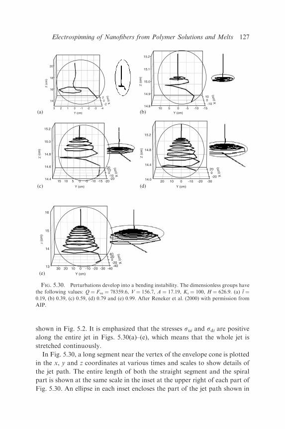
shown in Fig. 5.2. It is emphasized that the stresses sui and sdi are positive

along the entire jet in Figs. 5.30(a)–(e), which means that the whole jet is

stretched continuously.

In Fig. 5.30, a long segment near the vertex of the envelope cone is plotted

in the x, y and z coordinates at various times and scales to show details of

the jet path. The entire length of both the straight segment and the spiral

part is shown at the same scale in the inset at the upper right of each part of

Fig. 5.30. An ellipse in each inset encloses the part of the jet path shown in

14

16

18

20

-20

2

-4-3-2-10123

Z (

cm)

X (

cm)

Y (cm)

14.8

14.9

15.0

15.1

15.2

-100

10

-15-10-50510

Z (

cm)

X (

cm)

Y (cm)

14.4

14.6

14.8

15.0

15.2

-20-1001020

-20-15-10-5051015

Z (

cm)

X (

cm)

Y (cm)

14.0

14.4

14.8

15.2

-200

20

-30-20-1001020

Z (

cm)

X (

cm)

Y (cm)

13

14

15

16

-40-2002040

-40-30-20-100102030

z (c

m)

X (

cm)

Y (cm)

(a) (b)

(c) (d)

(e)

FIG. 5.30. Perturbations develop into a bending instability. The dimensionless groups have

the following values: Q ¼ Fve ¼ 78359.6, V ¼ 156.7, A ¼ 17.19, Ks ¼ 100, H ¼ 626.9. (a) t ¼

0:19; (b) 0.39, (c) 0.59, (d) 0.79 and (e) 0.99. After Reneker et al. (2000) with permission from

AIP.


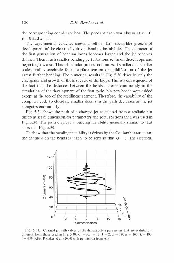
the corresponding coordinate box. The pendant drop was always at x ¼ 0,

y ¼ 0 and z ¼ h.

The experimental evidence shows a self-similar, fractal-like process of

development of the electrically driven bending instabilities. The diameter of

the first generation of bending loops becomes larger and the jet becomes

thinner. Then much smaller bending perturbations set in on these loops and

begin to grow also. This self-similar process continues at smaller and smaller

scales until viscoelastic force, surface tension or solidification of the jet

arrest further bending. The numerical results in Fig. 5.30 describe only the

emergence and growth of the first cycle of the loops. This is a consequence of

the fact that the distances between the beads increase enormously in the

simulation of the development of the first cycle. No new beads were added

except at the top of the rectilinear segment. Therefore, the capability of the

computer code to elucidate smaller details in the path decreases as the jet

elongates enormously.

Fig. 5.31 shows the path of a charged jet calculated from a realistic but

different set of dimensionless parameters and perturbations than was used in

Fig. 5.30. The path displays a bending instability generally similar to that

shown in Fig. 5.30.

To show that the bending instability is driven by the Coulomb interaction,

the charge e on the beads is taken to be zero so that Q ¼ 0. The electrical

0

20

40

60

80

100

120

-10

010

-15-10-50510

Z (

dim

ensi

onle

ss)

X(d

imen

sion

less

)

Y(dimensionless)

FIG. 5.31. Charged jet with values of the dimensionless parameters that are realistic but

different from those used in Fig. 5.30. Q ¼ Fve ¼ 12, V ¼ 2, A ¼ 0.9, Ks ¼ 100, H ¼ 100,

t ¼ 4:99: After Reneker et al. (2000) with permission from AIP.


driving force for the bending instability is then zero, but the other

parameters are exactly the same as those in Fig. 5.31. If a jet were to be

pulled downward by gravity, which can supply a downward component of

force that acts on the segment in the same way as the downward component

of the electrical force from the electrical field, one would expect the

uncharged jet to be almost straight in spite of the small perturbations

applied to it, since the perturbations would not develop into a bending

instability. The calculated result with the same parameters as those in Fig.

5.31, but Q ¼ 0, is in fact a straight jet growing downward, even at a later

time ðt ¼ 8:99Þ: Increasing the ratio of the surface tension to the Coulomb

force also stabilizes a charged jet. If A is increased to 9, by increasing the

surface tension while all the other parameters are kept the same as those in

Fig. 5.31 practically no bending occurs. The results for the gravity driven jet

and for the high-surface tension jet are not shown because the calculated jet

path cannot be distinguished from a straight line at the scale in Fig. 5.31.

2. Jet Path Calculated for the Electrically Driven Bending Instability

Accounting for Evaporation and Solidification

As was shown in Section V.J.1, the qualitative pattern of the jet behavior

in the electrospinning process can be drawn without accounting for

evaporation and solidification. A quantitative comparison with experiment

can be made only accounting for evaporation and solidification. Such a

comparison is the aim of the following sections. Also, a comparison between

the results obtained with and without accounting for evaporation and

solidification will be made here.

Calculations of the present work were done for an aqueous solution with an

initial 6% concentration of PEO studied experimentally as described in Section

V.B. The following values of the dimensional parameters were established: the

initial cross-sectional radius a0 ¼ 150mm the density r ¼ 103 kg m�3; the

surface tension s ¼ 0:07 kg s�2; the initial viscosity m0 ¼ 103 kg ðm sÞ�1; the

initial relaxation time y0 ¼ 10 ms; the charge density 1CL�1 and the distance

to the collecting plate h ¼ 20 cm. In the calculations of the present work, we

took the field strength U0/h ¼ 1.5kVm�1. In the experiment the electric field

was 50kVm�1. The values of the dimensionless groups introduced in Eqs.

(5.6), (5.65) and (5.69) are now based on the initial values of the dimensional

parameters and are equal to Q ¼ Fve ¼ 78359.57, V ¼ 47.02, A ¼ 17.19,

KS ¼ 100 and H ¼ 626.88, whereas Lel ¼ 0.319 cm. We also took the humidity

of 16.5%, cs1 ¼ 0:165; and the temperature of 201C. The best representation


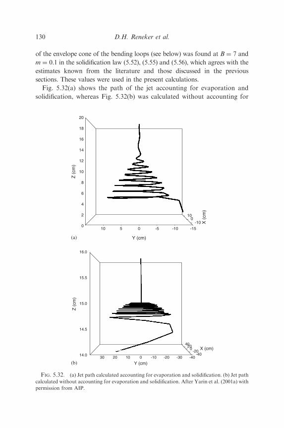
of the envelope cone of the bending loops (see below) was found at B ¼ 7 and

m ¼ 0.1 in the solidification law (5.52), (5.55) and (5.56), which agrees with the

estimates known from the literature and those discussed in the previous

sections. These values were used in the present calculations.

Fig. 5.32(a) shows the path of the jet accounting for evaporation and

solidification, whereas Fig. 5.32(b) was calculated without accounting for

0

2

4

6

8

10

12

14

16

18

20

-100

10

-15-10-50510

Z (

cm)

Y (cm)

14.0

14.5

15.0

15.5

16.0

-40-20

02040

-40-30-20-100102030

Z (

cm)

X (cm)

Y (cm)

(a)

X (

cm)

(b)

FIG. 5.32. (a) Jet path calculated accounting for evaporation and solidification. (b) Jet path

calculated without accounting for evaporation and solidification. After Yarin et al. (2001a) with



these effects. Owing to evaporation and solidification each loop of the jet

becomes more viscous with time, and its elastic modulus increases. As a

result, the resistance to bending increases, and the radius of the bending

loops in Fig. 5.32(a) (with evaporation and solidification) is smaller than

that of Fig. 5.32(b) (without evaporation and solidification). The radius of

the bending perturbations of the jet calculated accounting for the

evaporation and solidification effects is well comparable with that found

in the experiment (cf. Fig. 5.2), which is illustrated in the following section.

3. Envelope Cone

Shape of the envelope cone can be easily seen by a naked eye, or using a

camera with long exposure time (cf. Fig. 5.33). The two bright lines

bifurcating in Fig. 5.33 from a point emphasized by the arrow resulted from

a specular reflection of light from segments near the maximum lateral

excursion of each loop. Each loop moved downward during a long exposure

time of the camera and created the bright lines seen in Fig. 5.33, which

define the envelope cone of the bending jet during the electrospinning

process. For comparison with the results of the calculations, the generatrix

of the envelope cone in Fig. 5.33 is also represented in Fig. 5.34.

FIG. 5.33. Shape of the envelope cone created by the electrically driven bending instability.

The complicated image in the lower part of the figure is a consequence of the long exposure time

(�16ms) used to observe the envelope cone, and the time varying path of the jet in that region.

After Yarin et al. (2001a) with permission from AIP.


The calculations showed that the evaporation and solidification have a strong

effect on the predicted shape of the envelope cone. Two theoretical curves:

without evaporation and solidification, and with these effects accounted for

(m ¼ 0.1) are presented in Fig. 5.34. It is clearly seen that the result accounting

for evaporation and solidification agrees fairly well with the experimental data.

The envelope visible in the experiment does not extend beyond a radius of

about 3 cm, whereas the theory allowed for further growth of a radius until

10 cm. The reason may be that after the jet had solidified in the experiment, it

became much more rigid, i.e. unstretchable. On the other hand, in the theoretical

calculations the solidified jet is still described as a liquid (albeit highly viscous,

with a high-elastic modulus), which still allows for some additional stretching.

Actually, the comparison in Fig. 5.34 shows that the calculations should be

stopped as the radius of the envelope cone has achieved the value of 3–4 cm.

4. Jet Velocity

Downward velocity in the electrified jet was measured by following the

downward motion of a loop. The comparison of the experimental and

theoretical results is shown in Fig. 5.35. The velocity is practically

independent on time in both experiment and theory. The theoretical value

of the velocity overestimates the measured value by a factor of four. Given

the fact that the values of several governing parameters used in the

experiments are only an order of magnitude estimates, the discrepancy

represented by the factor of four is not dramatic.

Distance from spinneret (cm)0 2 4 6 8 10 12 14 16 18

Rad

ius

of th

e en

velo

pe c

one

(cm

)

0

2

4

6

8

10

Theory, withevaporation

Experiment

Theory, withoutevaporation

FIG. 5.34. Shape of the envelope cone: experiment vs. theory. Points show calculated radii

of successive loops. Experimental points were measured from a photograph. After Yarin et al.

(2001a) with permission from AIP.


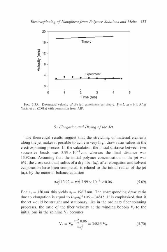
5. Elongation and Drying of the Jet

The theoretical results suggest that the stretching of material elements

along the jet makes it possible to achieve very high draw ratio values in the

electrospinning process. In the calculation the initial distance between two

successive beads was 3.99� 10�4 cm, whereas the final distance was

13.92 cm. Assuming that the initial polymer concentration in the jet was

6%, the cross-sectional radius of a dry fiber (af), after elongation and solvent

evaporation have been completed, is related to the initial radius of the jet

(a0), by the material balance equation

pa2f 13:92 ¼ pa2

0 3:99� 10�4 � 0:06. (5.69)

For a0 ¼ 150 mm this yields af ¼ 196.7 nm. The corresponding draw ratio

due to elongation is equal to (a0/af)20.06 ¼ 34815. It is emphasized that if

the jet would be straight and stationary, like in the ordinary fiber spinning

processes, the ratio of the fiber velocity at the winding bobbin Vf to the

initial one in the spinline V0 becomes

Vf ¼ V0pa2

0 0:06

pa2f

¼ 34815 V0. (5.70)

Time (ms)0 1 2 3 4 5

Vel

ocity

(m

/s)

0

4

8

12

16

20

Theory

Experiment

FIG. 5.35. Downward velocity of the jet: experiment vs. theory. B ¼ 7, m ¼ 0.1. After

Yarin et al. (2001a) with permission from AIP.


For the experimentally measured value of V0 ffi 0:1 m s�1 the velocity Vf

would be

Vf ¼ 3481:5 m s�1 ¼ 10 ðspeed soundÞ (5.71)

Obviously, this is not true. The paradoxical value of Vf in Eq. (5.71)

results from the fact that huge elongation of the fiber cannot be achieved at

the distance of about 10 cm along a straight line. The electrically driven

bending instability supplies the mechanism of strong elongation via fractal-

like looping which allows reduction of the final radius af to the range of

nanofibers, even though Vf ffi 1 m s�1:Fig. 5.36 shows the trajectories of two successive beads of the jet in the

course of electrospinning. The trajectories are shown by solid lines, and the

positions of the beads by black squares and circles. The lines that have

longer dashes connect the positions of the adjacent beads. To simplify, not

every connection is shown. The projections of the dashed line onto the X–Y

plane are shown by the lines with shorter dashes. The X–Y projections of the

bead positions are shown by gray squares or circles. The dashed lines

4

6

8

10

12

14

16

18

20

04

80 2 4 6 8 10

Z (

cm)

X (cm)

leading beadfollowing bead

Y (cm)

FIG. 5.36. Stretching of a segment of the jet. Each solid line represents a trajectory of one

of the two successive beads. The dashed lines represent the segment of the jet between the

successive beads. The length of the segment increases with time as a result of the jet stretching

during the course of electrospinning. B ¼ 7, m ¼ 0.1. The projections of the bead positions onto

the X–Y plane are shown by the gray symbols. After Yarin et al. (2001a) with permission from

AIP.


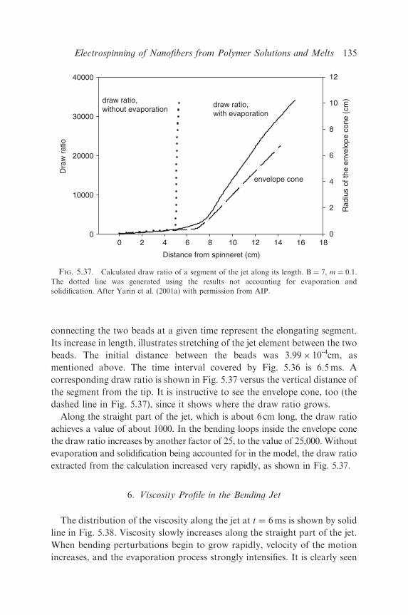
connecting the two beads at a given time represent the elongating segment.

Its increase in length, illustrates stretching of the jet element between the two

beads. The initial distance between the beads was 3.99� 10-4cm, as

mentioned above. The time interval covered by Fig. 5.36 is 6.5ms. A

corresponding draw ratio is shown in Fig. 5.37 versus the vertical distance of

the segment from the tip. It is instructive to see the envelope cone, too (the

dashed line in Fig. 5.37), since it shows where the draw ratio grows.

Along the straight part of the jet, which is about 6 cm long, the draw ratio

achieves a value of about 1000. In the bending loops inside the envelope cone

the draw ratio increases by another factor of 25, to the value of 25,000. Without

evaporation and solidification being accounted for in the model, the draw ratio

extracted from the calculation increased very rapidly, as shown in Fig. 5.37.

6. Viscosity Profile in the Bending Jet

The distribution of the viscosity along the jet at t ¼ 6ms is shown by solid

line in Fig. 5.38. Viscosity slowly increases along the straight part of the jet.

When bending perturbations begin to grow rapidly, velocity of the motion

increases, and the evaporation process strongly intensifies. It is clearly seen

Distance from spinneret (cm)

0 2 4 6 8 10 12 14 16 18

Dra

w r

atio

0

10000

20000

30000

40000

Rad

ius

of th

e en

velo

pe c

one

(cm

)

0

2

4

6

8

10

12

envelope cone

draw ratio,without evaporation

draw ratio,with evaporation

FIG. 5.37. Calculated draw ratio of a segment of the jet along its length. B ¼ 7, m ¼ 0.1.

The dotted line was generated using the results not accounting for evaporation and

solidification. After Yarin et al. (2001a) with permission from AIP.


when comparing the viscosity profile with that of the envelope cone shown

in Fig. 5.38 by the dashed line. Fast evaporation strongly increases the

polymer fraction in the jet, which leads to solidification manifested by the

appearance of the high-viscosity plateau at a distance of about 2 cm from

the beginning of the envelope cone. The calculation showed that at the

beginning of the plateau, nanofibers have already been formed, since the

cross-sectional radius of the fiber is already about 640 nm.

7. Longitudinal Strain Rate and Molecular Orientation

The high value of the area reduction ratio and the associated high

longitudinal strain rate imply that the macromolecules in the nanofibers

should be stretched and axially oriented. Most electrospun nanofibers, even

those made from a styrene–butadiene–styrene triblock copolymer, are

birefringent (Fong and Reneker, 1999).

The longitudinal strain rate was different at different places along the jet.

The longitudinal strain rate for three different parts of the jet was

determined.

(1) The jet velocity in the downward direction was determined from

the sequential images by determining the velocity of particular

Distance from spinneret (cm)0 2 4 6 8 10 12 14 16 18

Vis

cosi

ty, µ

(g/

(cm

. s))

0

200×103

400×103

600×103

800×103

1x106

Rad

ius

of th

e en

velo

pe c

one

(cm

)

0

2

4

6

8

10

12

envelope cone

viscosity

FIG. 5.38. Calculated viscosity along the jet; t ¼ 6ms, B ¼ 7 and m ¼ 0.1. The calculated

radius of the envelope cone continued to grow after the viscosity reached the plateau. After

Yarin et al. (2001a) with permission from AIP.


maxima of the growing bending instability and the length of the

straight segment. The length of the straight segment (Lz) was 5 cm

and the velocity was 1m s�1. Therefore, the longitudinal strain rate

was ðdLz=LzdtÞ;

dLz=Lz dt ¼ V dt=Lz dt ¼ V=Lz ¼ ð1 m s�1Þð1=0:05 mÞ ¼ 20 s�1,

(5.72)

which is a rough estimate of the strain rate in the straight segment

of the jet. Detailed measurements shown in Fig. 5.18 yield the

values of the order of several hundreds reciprocal seconds.

(2) The observation of expanding loops provided a second measure of

the longitudinal strain rate for the segment that formed the loop.

A typical loop grew from a diameter of 1 to 8mm in 7ms. The

resulting longitudinal strain rate in such a loop was 1000 s�1.

(3) The overall longitudinal strain rate can be estimated using the data

in Section V.J.5. The time that a typical segment of the electrospun

jet is in flight (dt) can be estimated as the distance between the

pendant droplet and the collector (20 cm) divided by the average

downward velocity of the jet (1m s�1). The resulting dt is 0.2 s. The

longitudinal strain rate is dz=ðdt zÞ; where z is the initial segment

length, and dz is the growth in length. Since dz is much greater

than z, dz is approximately the final segment length. The ratio dz/zwas around 105, and therefore the longitudinal strain rate was

around 0.5� 106s�1. Using the estimate, Eq. (5.72), we find that in

the straight segment the length of a liquid element has been

approximately doubled, and the cross-sectional radius decreased

by a factor of four. Then the longitudinal strain rate in the loops

becomes of the order of 105 s�1. The actual value will be lower due

to the effects of evaporation and solidification.

Theory suggests that the transformation from a random coil to a stretched

macromolecule occurs when the strain rate multiplied by the conformational

relaxation time of the molecule is greater than 0.5 (Chang and Lodge, 1972;

de Gennes, 1974). Since the relaxation time of the polymer solution is about

0.01 s–0.1 s, then dz/(dt z) multiplied by the relaxation time was equal to

10–104, which is much greater than 0.5. Therefore, the longitudinal flow in

the electrospun jet is strong, and the macromolecules are likely to be

stretched in the direction of the jet axis.


8. Theory of Branching on Electrospun Jets

An infinitely long static jet of incompressible fluid with a uniform circular

cross-section, in a radial electric field, is the theoretical model used in Yarin

et al. (2005) as a starting point to describe a mechanism that leads to quasi-

periodic branching of an electrospinning jet. This approximation is related

to the fact that branching takes place on the background of bending, albeit

quite independently of it (cf. Section V.B.2). The electrical conductivity is

supposed to be large enough to assume that excess charge is always at the

surface.

The surface of the jet can respond to the presence of the electrical

Maxwell forces in the following interesting way. If any element of the

charged surface moves outward in response to the electrical forces, the

motion of that element will extract energy from the electrical field, in order

to form a ‘‘hill’’. The lateral surface area associated with the growing hill

must increase because volume is conserved, since flow from the ends cannot

occur in an infinitely long jet of incompressible fluid. The energy required to

form the undulating surface of hills, saddle points and valleys is provided by

the electric field. The resulting static undulations may be quite complicated.

The distribution of electrical charge on the surface of the jet is similarly

complicated.

Consider a segment of a cylindrical fluid jet with a straight axis

surrounded by a coaxial hollow cylindrical electrode. The liquid in the jet

is assumed to be a perfect electrical conductor, which means that the time

intervals required for changes in the shape of the surface are much longer

than the characteristic charge relaxation time tC, which is of the order of

0.155� 10�2ms for acetone. If the jet were to be a perfect non-conductor of

electricity, the redistribution of charge on the surface that is required to

stabilize an undulating surface by an intricate balance of electrical and

surface tension forces might not be possible.

Assume that the surface of the jet is kept at an electrical potential j ¼ 0,

and the concentric cylindrical electrode is kept at j ¼ j0. Note that for a

solid circular cylinder, this condition defines both the charge per unit area

and the electric field normal to the surface of the cylinder, which are

parameters often used in electrical engineering and physics to characterize

the electrostatic conditions of this coaxial geometry, but that approach does

not encompass the changes in the shape of the surface that are considered in

this section.

To find a mathematical expression for these undulating shapes, the

solution of the partial differential equation that describes the shape of the


surface of the jet and the electric field in the linear approximation is written

as a two-dimensional Fourier series that depends on the azimuthal angle and

the distance along the axis of the jet. Substituting the assumed Fourier series

into the partial differential equation, and using the boundary conditions to

evaluate the coefficients of the various terms in the Fourier series leads to

the identification of terms in the series that are in equilibrium, static and

non-zero. The sum of these non-zero modes determines the shape of the

undulating surface of the jet. Since only a subset of the Fourier modes is

static, there is a finite wavelength associated with the static mode that has

the longest wavelength along the axis.

In the stability analysis in Yarin et al. (2005), which is related to the earlier

results of Saville (1971) and Yarin (1979), it is argued that the longest

allowed static wavelength along the jet axis leads to the observed quasi-

regular spacing of the branches.

A smooth jet with a circular cross-section is the only stable shape at low

electrical potential differences. Not every undulating shape can occur in

equilibrium as the potential is increased, but some static undulations of the

jet surface inevitably occur. Near the highest peaks of the static undulations,

shape perturbations, which increase the radius of curvature (cf. Fig. 5.39),

grow rapidly and give rise to branching.

The calculations were made for all four potentials for which measurements

were made, and the predicted branch spacings ‘N are compared with the

measured ones in Table 5.3 (Yarin et al., 2005). The predictions at the higher

voltage values (7.5 and 10kV) are commensurate with the measurements. The

comparison at the lower voltage values is not so good, especially at 5 kV,

which might be related to the wide distribution of observed spacings at the

lower voltage values caused by variations (perhaps a factor of 2) due to the

elongation of the distance between branches that occurs after the branches

start growing. The experimentally observed spacing distributions at 7.5 and

10kV suggest narrower distributions of the distance between branches.

K. MULTIPLE-JET ELECTROSPINNING

Electrospinning of multiple, mutually interacting jets was investigated in

Theron et al. (2005). Several experimental settings were used. In the first set-

up nine identical syringes, containing identical solutions, were arranged in a

3� 3 matrix (Fig. 5.40(a). In the second, the set-up in Fig. 5.40(b), nine and

seven syringes were arranged in a row. Numerical simulation of the

multiple-jet electrospinning was conducted within the framework the model

described in Sections V.C–V.J.


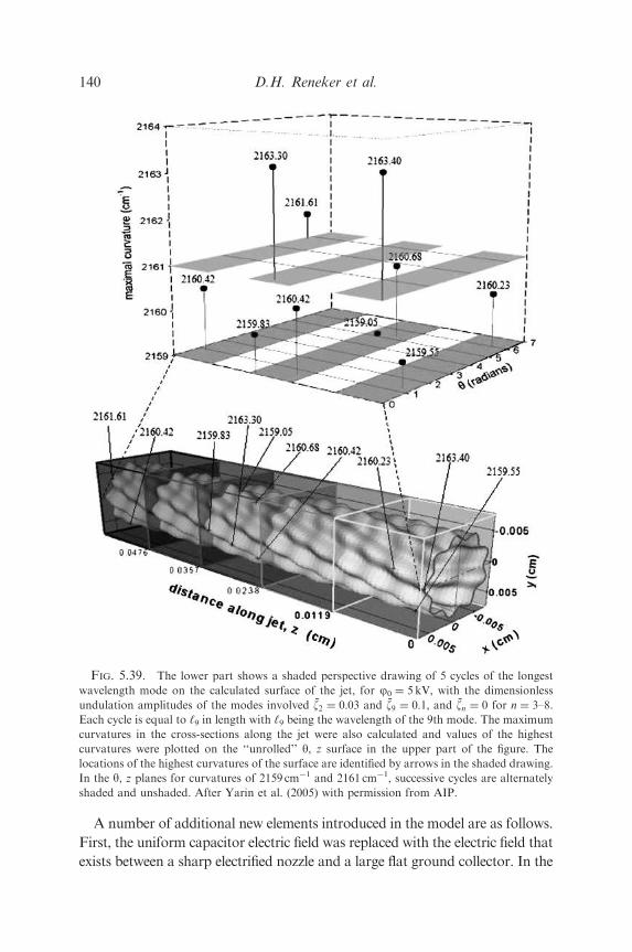
A number of additional new elements introduced in the model are as follows.

First, the uniform capacitor electric field was replaced with the electric field that

exists between a sharp electrified nozzle and a large flat ground collector. In the

FIG. 5.39. The lower part shows a shaded perspective drawing of 5 cycles of the longest

wavelength mode on the calculated surface of the jet, for j0 ¼ 5 kV, with the dimensionless

undulation amplitudes of the modes involved z2 ¼ 0:03 and z9 ¼ 0:1; and zn ¼ 0 for n ¼ 3–8.

Each cycle is equal to ‘9 in length with ‘9 being the wavelength of the 9th mode. The maximum

curvatures in the cross-sections along the jet were also calculated and values of the highest

curvatures were plotted on the ‘‘unrolled’’ y, z surface in the upper part of the figure. The

locations of the highest curvatures of the surface are identified by arrows in the shaded drawing.

In the y, z planes for curvatures of 2159 cm�1 and 2161 cm�1, successive cycles are alternately

shaded and unshaded. After Yarin et al. (2005) with permission from AIP.


simplest form this field can be represented by the field between a point-wise

charge opposite to a conducting plate (or a mirror image of a charge of an

opposite sign). Also, mutual Coulombic interactions between the charged jet

elements were accounted not only for a given jet, but for all the jets in the array.

To describe the rheological behavior of polymer solutions, the non-linear UCM

model was used in addition to the linear Maxwell model.

In all the cases, viscosity m ¼ 100P and the relaxation time y ¼ 0.1 s were

used in accordance with the data of Reznik et al. (2004). It was demonstrated

experimentally and with the help of numerical simulations that the mutual

Coulombic interactions influence the paths of individual electrified jets in

electrospinning. Mutual repulsion of the jets is highlighted by arrows in Figs.

5.40(a), (b) and is reproduced by the simulation results shown in Fig. 5.41.

Furthermore, the semi-vertical angle of the electrospinning envelope cones, of

the two jets on the edges, is larger than for the inner jets (#2–8 in Fig. 5.40(b)).

The values of the latter angles were obtained by measuring the semi-angle

between the two bright lines bifurcating for a specific jet envelope in Fig.

5.40(b). In Fig. 5.40(b), the measured angle for jet #5 is indicated by a double-

headed arrow. The semi-vertical angle of the electrospinning envelope for the

inner jets lies between 251 and 301, whereas for jet #1 it is about 401.

When rotating Fig. 5.40(b) by 901, the semi-vertical angle of the envelope

cone in the direction perpendicular to the line on which the nozzles are

located is revealed. The latter angle, estimated from Fig. 5.40(c), is between

501 and 751. This confirms that the inner envelope cones are, in fact,

squeezed along the line on which the nozzles are located. A similar result is

revealed by the simulations (cf. Fig. 5.41(c)). Although the electrospinning

envelopes are squeezed, the electrically driven bending instability of all the

jets is similar to the one familiar for single jets. The results of the modeling

suggest that both the non-linear UCM model and the linear Maxwell model

provide a reasonable and quite close description of the viscoelastic behavior

of jets in electrospinning.

Table 5.3. The calculated and observed distance between branches along thejet.

Applied voltage (kV) Average electric field

between tip and

collector (V/mm)

‘N (calculated) (mm) ‘N (measured) (mm)

4 57 379 294

5 71 119 353

7.5 107 118 118

10 143 124 118


FIG. 5.40. (a) A photograph of a nine-jet electrospinning process where the jets were

arranged in a 3� 3 matrix (set-up A). The photograph was taken with a slow shutter speed

(200ms). Arrows indicate the three-dimensional directions of the jets’ axes. The distance, ds,

between the nozzles in the image was 5 cm. (b) Photographs were taken at long exposure times

(200ms) of a nine-jet electrospinning process using set-up B. The distance between the

individual syringes ds ¼ 4 cm. Front view of jets ]1–9 with arrows to indicate the direction of the

main axes of the electrospinning envelopes. (c) A side view of all the jets in set-up B. Jet #1 is the

foremost jet in the image. After Theron et al. (2005) with permission from Elsevier.


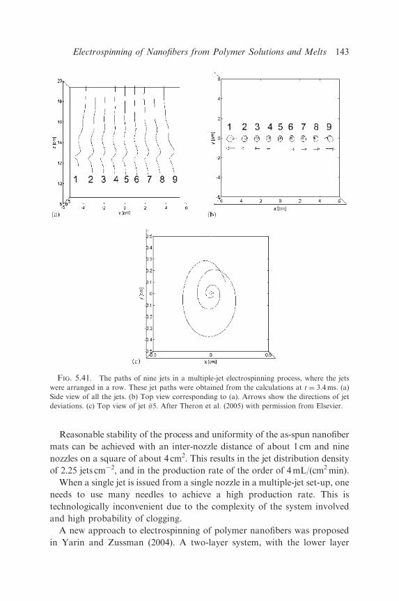
Reasonable stability of the process and uniformity of the as-spun nanofiber

mats can be achieved with an inter-nozzle distance of about 1 cm and nine

nozzles on a square of about 4 cm2. This results in the jet distribution density

of 2.25 jets cm�2, and in the production rate of the order of 4mL/(cm2min).

When a single jet is issued from a single nozzle in a multiple-jet set-up, one

needs to use many needles to achieve a high production rate. This is

technologically inconvenient due to the complexity of the system involved

and high probability of clogging.

A new approach to electrospinning of polymer nanofibers was proposed

in Yarin and Zussman (2004). A two-layer system, with the lower layer

FIG. 5.41. The paths of nine jets in a multiple-jet electrospinning process, where the jets

were arranged in a row. These jet paths were obtained from the calculations at t ¼ 3.4ms. (a)

Side view of all the jets. (b) Top view corresponding to (a). Arrows show the directions of jet

deviations. (c) Top view of jet #5. After Theron et al. (2005) with permission from Elsevier.


being a ferromagnetic suspension and the upper layer a polymer solution,

was subjected to a normal magnetic field provided by a permanent magnet

or a coil (Fig. 5.42). As a result, steady vertical spikes of magnetic

suspension perturbed the inter-layer interface, as well as the free surface of

the uppermost polymer layer. When a normal electric field was applied in

addition, the perturbations of the free surface become sites of jetting

directed upward. Multiple-electrified jets underwent strong stretching by the

electric field and bending instability, solvent evaporated and solidified

nanofibers were deposited on the upper counter-electrode, as in an ordinary

electrospinning process. The jet density in such a process was estimated as 26

jets cm�2 instead of the above-mentioned value of 2.25 jets cm�2. As a result,

a 12-fold increase in the production rate is expected when this method is

used instead of separate nozzles. In addition, the design problems related to

multiple nozzles, as well as clogging can be eliminated.

L. CONCLUDING REMARKS

The entire electrospinning process and the electrically driven bending

instabilities of an electrospun fluid can each be viewed as particular

FIG. 5.42. Schematic drawing of the experimental setup. (a) Layer of magnetic liquid, (b)

layer of polymer solution, (c) counter-electrode located at a distance H from the free surface of

the polymer, (d) electrode submerged into magnetic fluid, (e) high-voltage source, and (f) strong

permanent magnet or electromagnet. After Yarin and Zussman (2004) with permission from

Elsevier.


examples of the very general Earnshaw theorem in electrostatics. This

theorem leads to the conclusion that it is impossible to create a stable

structure in which the elements of the structure interact only by Coulomb’s

law. Charges on or embedded in a polymer fluid move the fluid in quite

complicated ways to reduce their Coulomb interaction energy. Electrospin-

ning, and perhaps other useful processes, utilizes this behavior to produce

interesting and useful polymer objects.

The localized approximation introduced in the present section utilized a

far-reaching analogy between the electrically driven bending instability in

the electrospinning process and the aerodynamically driven bending

instability studied before. The quasi-one-dimensional partial differential

equations of the jet dynamics that describe the paths of the electrified jets in

electrospinning were established.

A reasonable quantitative description of the experimental data was

achieved, which allows one to calculate the shape of the envelope cone,

which surrounds the bending loops of the jet in electrospinning. The

downward velocity of the jet can also be calculated to be within an order of

magnitude of the observed velocity. The theoretical results also allow for the

calculation of the elongation of material elements of the jet. The calculated

results also illustrate the increase in viscosity of segments of the jet as the

solvent evaporates during the course of electrospinning. Multiple-jet

configurations were studied both experimentally and via numerical

modeling.

It is emphasized that presently, information on the rheological material

behavior of polymer solution being elongated at the rate and other

conditions encountered during electrospinning, is rather scarce. Data on

evaporation and solidification of polymer solutions in the electrospinning

process are practically unavailable. Therefore, at present a number of

parameters in the simulations can only be estimated by the order of

magnitude, or found from experimental observations of the electrospinning

process. Material science data acquired for the electrospinning process will

allow researchers to avoid such obstacles in future. A more detailed

description of the nature of the solvents (in many cases, mixtures of several

miscible fluids with a variable evaporation rate) may also be very helpful for

a further upgrading of the modeling capabilities.

Note also that a physically similar approach to bending instability of a

single jet of inelastic Newtonian viscous liquids was developed in Shin et al.

(2001a,b), Hohman et al. (2001a,b) and Fridrikh et al. (2003). In these works

the phenomenon was called whipping instability.


VI. Scientific and Technological Challenges in Producing Nanofibers with

Desirable Characteristics and Properties

Electrospinning has been shown to be an effective method for the

production of nanofibers. For most applications, it is desirable to control, in

addition to the diameter of the fibers, also the architecture, the internal

composition, the internal morphology and the surface topology as well as

fibers alignment in a structure. Porous fibers are of interest, for instance, for

filter applications. Core-shell fibers, or fibers which are hollow, are of

interest for storage, release systems and insulation. A given surface topology

and chemical structure will affect, for instance, the wetting behavior (super-

hydrophobicity), as well as specific adsorption processes (Busscher et al.,

1984; Jiang et al., 2004; Ma et al., 2005; Oner and McCarthy, 2000;

Youngblood and McCarthy, 1999), and it will couple very effectively to the

surrounding matrix in the case of reinforcement (Huang et al., 2003). The

objective is to tailor the fiber formation during electrospinning in such a way

that fibers with specific diameters, architectures, internal structures and

surface topologies are manufactured and aligned specifically for the targeted

application.

A further objective is the inclusion of additives – drugs, catalysts (i.e. TiO2

nanoparticles or enzymes), non-linear optical materials, electrically con-

ducting and photosensitive materials, chromophores, for example into the

fibers, possibly only in well-defined compartments within the fibers.

Chemical modifications and functionalizations of fibers, again directed at

optimizing the properties for specific applications, are highly desirable

(Kedem et al., 2005; Kim et al., 2005a; Li et al., 2005).

First successes in preparation of conductive and photosensitive nanofibers

from electronic and photonic polymers (Drew et al., 2002; MacDiarmid et

al., 2001; MacDiarmid, 2002; Norris et al., 2000) show that electrically

conducting and light-emitting nanofibers and nanotubes are achievable via

electrospinning.

Electrical conductivity and strength of nanofibers are significantly

improved when single- and multi-wall carbon nanotubes, CNTs (Rakov,

2000) are incorporated into them. The attempts in this direction show that

nanofibers containing CNTs can be electrospun from a polymer-based

solution of CNTs (Dror et al., 2003; Ko et al., 2003; Seoul et al., 2003;

Salalha et al., 2004; Ye et al., 2004). Both multi-walled (MWCNT) and

single-walled (SWCNT) carbon nanotubes were oriented and embedded

inside nanofibers during electrospinning. The most important issue to be

tackled when electrospinning polymer-CNT solutions is the achievement of


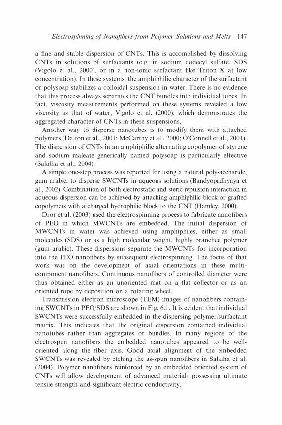
a fine and stable dispersion of CNTs. This is accomplished by dissolving

CNTs in solutions of surfactants (e.g. in sodium dodecyl sulfate, SDS

(Vigolo et al., 2000), or in a non-ionic surfactant like Triton X at low

concentration). In these systems, the amphiphilic character of the surfactant

or polysoap stabilizes a colloidal suspension in water. There is no evidence

that this process always separates the CNT bundles into individual tubes. In

fact, viscosity measurements performed on these systems revealed a low

viscosity as that of water, Vigolo et al. (2000), which demonstrates the

aggregated character of CNTs in these suspensions.

Another way to disperse nanotubes is to modify them with attached

polymers (Dalton et al., 2001; McCarthy et al., 2000; O’Connell et al., 2001).

The dispersion of CNTs in an amphiphilic alternating copolymer of styrene

and sodium maleate generically named polysoap is particularly effective

(Salalha et al., 2004).

A simple one-step process was reported for using a natural polysaccharide,

gum arabic, to disperse SWCNTs in aqueous solutions (Bandyopadhyaya et

al., 2002). Combination of both electrostatic and steric repulsion interaction in

aqueous dispersion can be achieved by attaching amphiphilic block or grafted

copolymers with a charged hydrophilic block to the CNT (Hamley, 2000).

Dror et al. (2003) used the electrospinning process to fabricate nanofibers

of PEO in which MWCNTs are embedded. The initial dispersion of

MWCNTs in water was achieved using amphiphiles, either as small

molecules (SDS) or as a high molecular weight, highly branched polymer

(gum arabic). These dispersions separate the MWCNTs for incorporation

into the PEO nanofibers by subsequent electrospinning. The focus of that

work was on the development of axial orientations in these multi-

component nanofibers. Continuous nanofibers of controlled diameter were

thus obtained either as an unoriented mat on a flat collector or as an

oriented rope by deposition on a rotating wheel.

Transmission electron microscope (TEM) images of nanofibers contain-

ing SWCNTs in PEO/SDS are shown in Fig. 6.1. It is evident that individual

SWCNTs were successfully embedded in the dispersing polymer/surfactant

matrix. This indicates that the original dispersion contained individual

nanotubes rather than aggregates or bundles. In many regions of the

electrospun nanofibers the embedded nanotubes appeared to be well-

oriented along the fiber axis. Good axial alignment of the embedded

SWCNTs was revealed by etching the as-spun nanofibers in Salalha et al.

(2004). Polymer nanofibers reinforced by an embedded oriented system of

CNTs will allow development of advanced materials possessing ultimate

tensile strength and significant electric conductivity.


Ge et al. (2004) developed highly oriented, large area continuous

composite nanofiber sheets made from surface-oxidized MWCNTs and

polyacrylonitrile (PAN) using electrospinning (Fig. 6.2). They reported the

highest degree of orientation of nanotubes in electrospun composite

nanofibers, which was determined with transmission electron microscopy

and electron diffraction. This degree of orientation in the electrospun PAN/

MWCNTs nanofiber sheets approaches that observed in the PAN/SWCNT

microfibers made by a dry-jet spinning method when the draw ratio reaches

the value of 4.3. They observed that the orientation of the CNTs within the

nanofibers was much higher than that of the PAN polymer crystal matrix as

detected by two-dimensional wide-angle X-ray diffraction (WAXD)

experiments. This suggests that not only jet elongation but also the slow

relaxations of the CNTs in the nanofibers are determining factors in the

orientation of CNTs. They revealed that the formation of charge transfer

complexes between the surface-oxidized nanotubes and negatively charged

functional groups in PAN during electrospinning leads to a strong

interfacial bonding between the nanotubes and surrounding polymer chains.

As a result of the highly anisotropic orientation and the formation of

1st

Overlap

2nd

FIG. 6.1. TEM image of composite nanofibers after etching in oxygen flow for 1min.

Bar ¼ 50 nm. A catalyst particle is seen on the left. After Salalha et al. (2004) with permission

from ACS.


complexes, the composite nanofiber sheets possessed enhanced electrical

conductivity, mechanical properties, thermal deformation temperature,

thermal stability and dimensional stability.

Hou and Reneker (2004) reported electrospun PAN nanofibers carbonized

and used as substrates for the formation of MWCNTs (Fig. 6.3). The

MWCNTs were formed by an ion-catalyzed growth mechanism. Electrospun

polymer nanofibers, produced using electrospinning, were made with diameters

FIG. 6.2. High magnification bright field TEM images of electrospun MWCNT/PAN

composite nanofibers containing (a) 10wt% and (b) 20wt% oxidized MWCNTs (the scale bar

of 100 nm). The inset in part (a) is an SAED pattern obtained from this nanofiber. After Ge et

al. (2004) with permission from ACS.

FIG. 6.3. Transmission electron micrographs of carbon nanostructures. (a) Long, slightly

curved carbon nanotubes formed at 8501C, (b) Curved and bent CNTs formed at 7001C. After

Hou and Reneker (2004) with permission from Wiley-VCH Verlag.


ranging from a few nanometers to several micrometers and collected in a highly

porous thin sheet. Multi-walled CNTs with metal particles on the tips grown on

such carbonized nanofiber substrates form a characteristic hierarchical

structure. This unique hierachical carbon structure, with dimensions that can

be controlled during synthesis, promises to become important in fuel-cells,

redox–reaction electrodes and in nanoscale engineering of other systems in

which electrical, mechanical and chemical interactions are integrated to

produce macroscale effects.

Conducting and photosensitive nanofibers can be obtained not only by

electrospinning, but also via different chemical and electrochemical synthesis

methods and template methods (Jerome et al., 1999; Demoustier-Champagne

et al., 1999; Wan et al., 1999; Hsu et al., 1999; Pomfret et al., 1999). However,

these nanofibers are always very short (� several mm) as compared to the

electrospun nanofibers (�10 cm and more).

Magnetic nanoparticles were embedded in the electrospun nanofiber mats

in Li et al., (2003), Yang et al. (2003) and Wang et al. (2004a). Magnetic-

field-responsive non-woven electrospun fabrics were produced.

Piezoelectric polymer poly(vinylidene fluoride), PVDF, which also has such

properties as pyroelectricity and ferroelectricity was successfully electrospun

in Bates et al. (2003), Yang et al. (2003) and Gupta and Wilkes (2003).

Beaded electrospun nanofibers result from capillary instability in the

process where polymer concentration, molecular weight or electric charge,

are insufficient. Lee et al. (2002, 2003c) showed that bead formation can be

controlled by using different solvents or solvent compositions. Fong et al.

(1999) examined other parameters, including reduction of charge on the jet,

which is very effective in producing beads. Beaded electrospun nanofiber

mats represent a perfect superhydrophobic surface (Jiang et al., 2004)

attractive for many applications. Beads appear to be helpful to strengthen

binding between the fibers and a matrix in fiber-reinforced composites

(Huang et al., 2003).

Some additional details on scientific and technological challenges related to

electrospinning of biofunctional, conducting and photosensitive nanofibers,

will be given below in the subsections devoted to these particular topics.

To overcome technological challenges in fabrication of microdevices,

techniques for in situ alignment of as-spun nanofibers/nanotubes using

electrostatic repulsion forces have recently been demonstrated (Theron et al.,

2001; Deitzel et al., 2001; Zussman et al., 2003b; Sundaray et al., 2004; Li

et al., 2004).

A sketch of the experimental apparatus used by Theron et al. (2001) and

Zussman et al. (2003b) is shown in Fig. 6.4. The jet flowed downward from


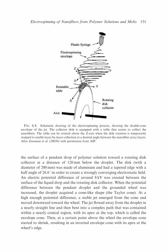
the surface of a pendant drop of polymer solution toward a rotating disk

collector at a distance of 120mm below the droplet. The disk (with a

diameter of 200mm) was made of aluminum and had a tapered edge with a

half angle of 26.61 in order to create a strongly converging electrostatic field.

An electric potential difference of around 8 kV was created between the

surface of the liquid drop and the rotating disk collector. When the potential

difference between the pendant droplet and the grounded wheel was

increased, the droplet acquired a cone-like shape (the Taylor cone). At a

high enough potential difference, a stable jet emerged from the cone and

moved downward toward the wheel. The jet flowed away from the droplet in

a nearly straight line and then bent into a complex path that was contained

within a nearly conical region, with its apex at the top, which is called the

envelope cone. Then, at a certain point above the wheel the envelope cone

started to shrink, resulting in an inverted envelope cone with its apex at the

wheel’s edge.

FIG. 6.4. Schematic drawing of the electrospinning process, showing the double-cone

envelope of the jet. The collector disk is equipped with a table that assists to collect the

nanofibers. The table can be rotated about the Z-axis when the disk rotation is temporarily

stopped to enable layer-by-layer collection at a desired angle between the nanofiber array layers.

After Zussman et al. (2003b) with permission from AIP.


During the electrospinning process, the disk was rotated at a constant

speed to collect the developing nanofibers onto its sharp edge. The linear

speed at the tip of the disk collector was V ¼ 11m s�1. As the as-spun fiber

reached the wheel’s edge, it was wound around the wheel.

A small table (5� 4mm) made of aluminum was attached to the disk edge

to facilitate the collection of the nanofibers and to detach them further on.

The table can be rotated about its Z-axis when the disk rotation is

temporarily stopped, hence the direction of the collected nanofibers can be

controlled. The nanofibers were collected over a 10 s period. The resulting

two-dimensional nanofiber arrays are shown in Fig. 6.5. The diameter of the

nanofibers was not uniform and varies from 100 to 300 nm in Fig. 6.5(a) and

from 200 to 400 nm in Fig. 6.5(b). The separation between the parallel

nanofibers also varies from 1 to 2 mm in Fig. 6.5(a) and from 1 to 1.5 mm in

Fig. 6.5(b). Typical three-dimensional nanofiber arrays (crossbars) are

depicted in Fig. 6.6. A single junction is shown in Fig. 6.7. The collected

nanofibers show a high order of alignment. The diameter of the nanofibers

in this case is also non-uniform and varies in the range 10–80 nm. When

nanofibers were electrospun onto the wheel’s sharp edge without the table,

nanoropes of nanofibers were obtained. A typical image of a rope of

nanofibers is shown in Fig. 6.8 (Theron et al., 2001). The duration of the

collection process was 60 s. The rope was manually detached from the wheel

edge. Two HR-SEM images of nanoropes are shown in Fig. 6.9. The

nanofibers are in contact, and nearly parallel for long distances.

Arrays similar to those shown in Figs. 6.5–6.7 are periodic arrays of

dielectric scatterers in a homogeneous dielectric matrix. Such arrays can

interact strongly with photons, which have commensurate wavelengths.

Such photonic structures have band structures, localized defect modes and

surface modes that can interact with and modify or direct photons. A variety

of novel applications of nanofibers and nanotubes in such fields as

microelectronics, telecommunications, solar energy conversion, medical

and pharmaceutical industry are developing rapidly.

For short nanofibers and nanowires prepared by methods other than

electrospinning, various assembly methods were proposed, e.g. electric-field

assisted assembly (Smith et al., 2000) and micro-fluidics methods (Huang et

al., 2001b).

Core-shell nano/meso fibers were first produced by co-electrospinning of

two materials in Sun et al. (2003). Essentially, the same process was adopted

elsewhere (Li and Xia 2004a,b; Loscertales et al., 2004; Yu et al., 2004;

Zhang et al., 2004). In this approach two different solutions flow through

concentric annular nozzles (Fig. 6.10). The experiments showed that for a


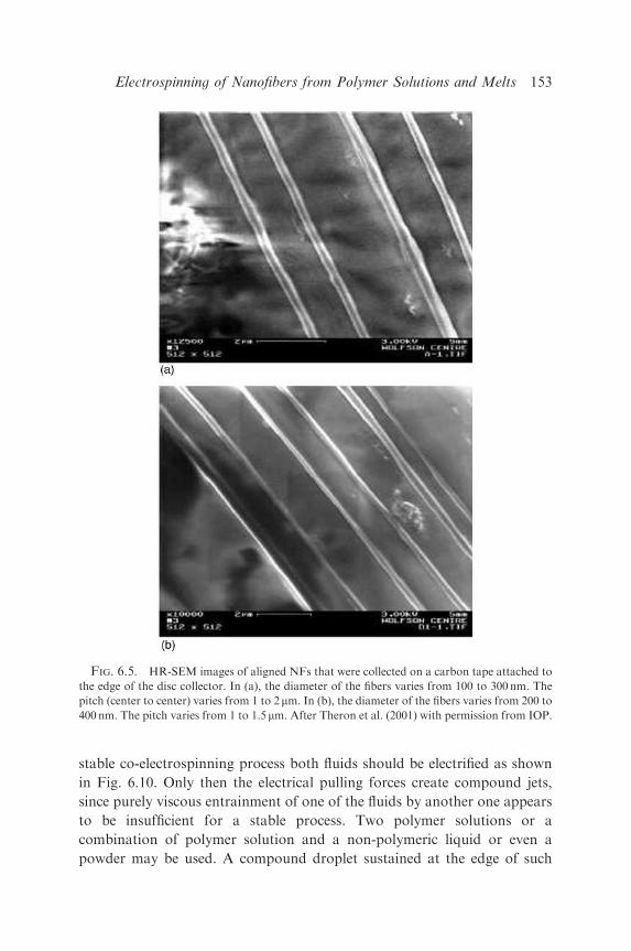
stable co-electrospinning process both fluids should be electrified as shown

in Fig. 6.10. Only then the electrical pulling forces create compound jets,

since purely viscous entrainment of one of the fluids by another one appears

to be insufficient for a stable process. Two polymer solutions or a

combination of polymer solution and a non-polymeric liquid or even a

powder may be used. A compound droplet sustained at the edge of such

FIG. 6.5. HR-SEM images of aligned NFs that were collected on a carbon tape attached to

the edge of the disc collector. In (a), the diameter of the fibers varies from 100 to 300 nm. The

pitch (center to center) varies from 1 to 2mm. In (b), the diameter of the fibers varies from 200 to

400 nm. The pitch varies from 1 to 1.5 mm. After Theron et al. (2001) with permission from IOP.


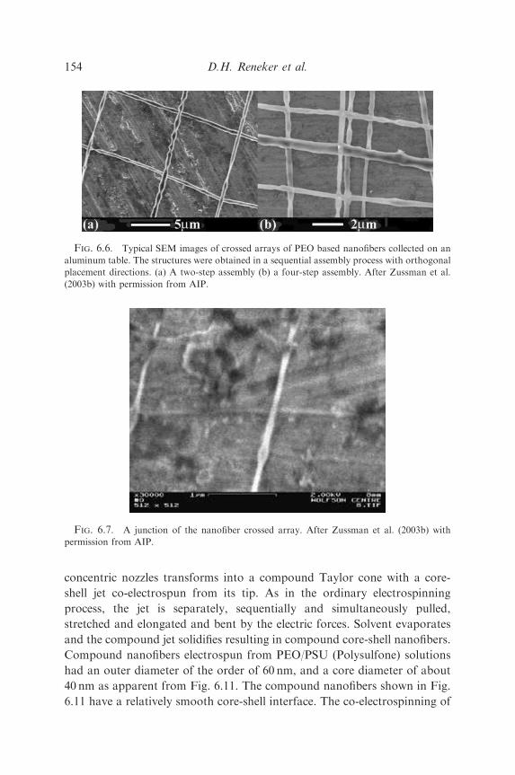
concentric nozzles transforms into a compound Taylor cone with a core-

shell jet co-electrospun from its tip. As in the ordinary electrospinning

process, the jet is separately, sequentially and simultaneously pulled,

stretched and elongated and bent by the electric forces. Solvent evaporates

and the compound jet solidifies resulting in compound core-shell nanofibers.

Compound nanofibers electrospun from PEO/PSU (Polysulfone) solutions

had an outer diameter of the order of 60 nm, and a core diameter of about

40 nm as apparent from Fig. 6.11. The compound nanofibers shown in Fig.

6.11 have a relatively smooth core-shell interface. The co-electrospinning of

FIG. 6.6. Typical SEM images of crossed arrays of PEO based nanofibers collected on an

aluminum table. The structures were obtained in a sequential assembly process with orthogonal

placement directions. (a) A two-step assembly (b) a four-step assembly. After Zussman et al.

(2003b) with permission from AIP.

FIG. 6.7. A junction of the nanofiber crossed array. After Zussman et al. (2003b) with



fluids is very versatile and will certainly foster new materials design. It can

also result in a two-stage method of fabrication of hollow nanofibers

(nanotubes) instead of the previously used three-stage one (Bognitzki et al.,

2000, 2001; Liu et al., 2002). Co-electrospinning should be followed by a

selective removal of the core material in the compound fiber via selective

solvents or heat treatment. Calcination and pyrolysis of polymers containing

metal atoms transform nanofibers and nanotubes into ceramic, and metal

ones (Liu et al., 2002; Li and Xia, 2003, 2004b; Li et al., 2004).

Carbonization of co-electrospun nanofibers yields turbostratic carbon

FIG. 6.8. A rope of aligned NFs manually pulled from the collector. Almost all the NFs

were collected on the edge of the sharpened disc collector. After Theron et al. (2001) with

permission from IOP.

FIG. 6.9. Typical HR–SEM images of two ropes of aligned NFs. The density is about 100

NFs mm�2. After Theron et al. (2001) with permission from IOP.


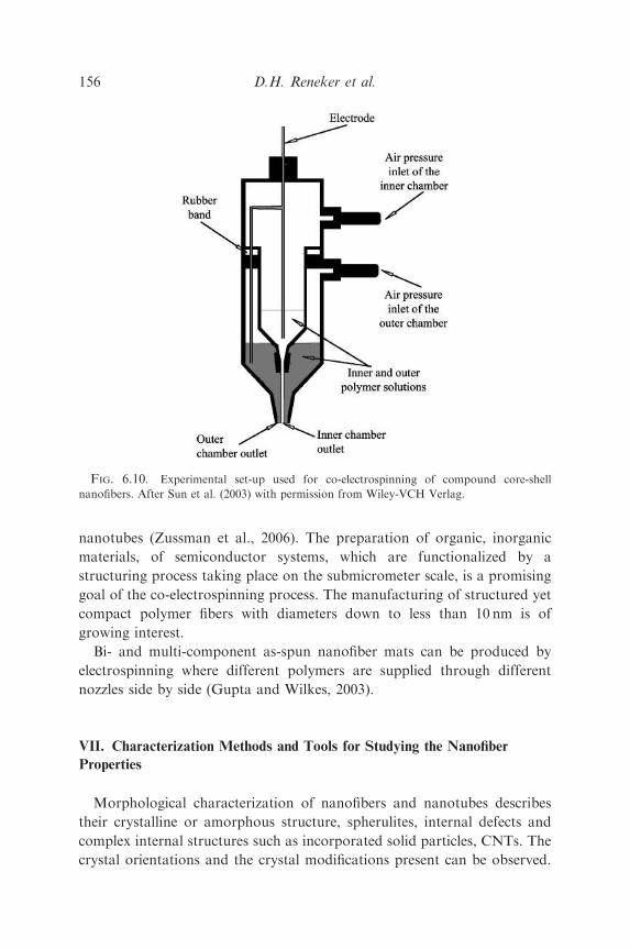
nanotubes (Zussman et al., 2006). The preparation of organic, inorganic

materials, of semiconductor systems, which are functionalized by a

structuring process taking place on the submicrometer scale, is a promising

goal of the co-electrospinning process. The manufacturing of structured yet

compact polymer fibers with diameters down to less than 10 nm is of

growing interest.

Bi- and multi-component as-spun nanofiber mats can be produced by

electrospinning where different polymers are supplied through different

nozzles side by side (Gupta and Wilkes, 2003).

VII. Characterization Methods and Tools for Studying the Nanofiber

Properties

Morphological characterization of nanofibers and nanotubes describes

their crystalline or amorphous structure, spherulites, internal defects and

complex internal structures such as incorporated solid particles, CNTs. The

crystal orientations and the crystal modifications present can be observed.

FIG. 6.10. Experimental set-up used for co-electrospinning of compound core-shell

nanofibers. After Sun et al. (2003) with permission from Wiley-VCH Verlag.


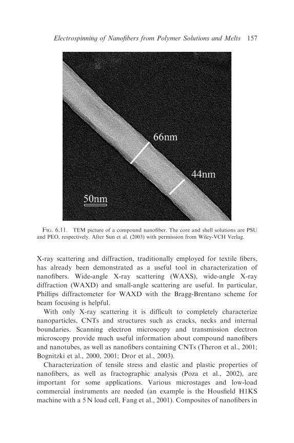
X-ray scattering and diffraction, traditionally employed for textile fibers,

has already been demonstrated as a useful tool in characterization of

nanofibers. Wide-angle X-ray scattering (WAXS), wide-angle X-ray

diffraction (WAXD) and small-angle scattering are useful. In particular,

Phillips diffractometer for WAXD with the Bragg-Brentano scheme for

beam focusing is helpful.

With only X-ray scattering it is difficult to completely characterize

nanoparticles, CNTs and structures such as cracks, necks and internal

boundaries. Scanning electron microscopy and transmission electron

microscopy provide much useful information about compound nanofibers

and nanotubes, as well as nanofibers containing CNTs (Theron et al., 2001;

Bognitzki et al., 2000, 2001; Dror et al., 2003).

Characterization of tensile stress and elastic and plastic properties of

nanofibers, as well as fractographic analysis (Poza et al., 2002), are

important for some applications. Various microstages and low-load

commercial instruments are needed (an example is the Housfield H1KS

machine with a 5N load cell, Fang et al., 2001). Composites of nanofibers in

FIG. 6.11. TEM picture of a compound nanofiber. The core and shell solutions are PSU

and PEO, respectively. After Sun et al. (2003) with permission from Wiley-VCH Verlag.


epoxy resin were tested using a double torsion fracture method in Kim and

Reneker (1999) and Dzenis (2004). Three points bending tests were carried

out using atomic force microscopy (Cuenot et al., 2000). Atomic force

microscope was also used to measure nanofiber dimensions and nanofiber-

array structures by Theron et al. (2001). Using microstages and tensile

machines (even the smallest ones), it is possible to make measurements only

with samples of non-woven nanofiber-based materials or oriented nanofiber

ropes (Theron et al., 2001). At present appropriate methods for observing

mechanical properties of a single nanofiber are being developed (Gu et al.,

2005; Inai et al., 2005; Kim et al., 2005b; Tan and Lim, 2004; Tan et al.,

2005, Zussman et al., (2006)).

Mechanical properties of electrospun fiber mats of polyblends of

poly(vinyl chloride) and polyurethane, PVC/PU, yield the Young’s modulus

up to 11.8MPa, the yield stress of 1.03MPa, the ultimate tensile stress of

3.73MPa and the elongation at break of 456% for 50/50 blends (Lee et al.,

2003b). For blends with higher content of PU, fully elastic behavior was

recorded up to the ultimate strength of 7.04MPa, and the elongation at

break of 1210% for pure PU mats. The Young’s modulus of the PU mats

was, however, much lower, namely 0.62MPa (Lee et al., 2003b). For non-

woven PU mats, the ultimate tensile stress of the order of 40MPa at the

elongation of about 700% was reported (Pedicini and Farris 2003). For non-

woven mats of poly(trimethylene terephthalate), PTT, nanofibers with

diameters ranging from 200 to 600 nm the ultimate tensile stress was about

4MPa at an elongation of about 300% (Khil et al., 2004). For mats of

gelatin nanofibers with diameters in the range from 100 to 340 nm, the

tensile modulus was of the order of 117–134MPa and the ultimate tensile

strength was in the range from 2.93 to 3.40MPa (Huang et al., 2004).

A natural material, spider silk, is both strong and biologically compatible

in certain cases (Lazaris et al., 2002; Poza et al., 2002). Spider dragline silk is

stronger than Kevlar and stretches better than nylon. This combination of

properties is seen in no other fiber. Numerous trials to domesticate spiders

and to raise spiders on a farm have not achieved success. However, there is a

way to utilize spider silk, which was recently developed via gene engineering

and polymer science. Spider dragline silk genes were spliced into mammalian

cells. It was shown that this resulted in secreting soluble silk proteins outside

the cells where they could easily be collected (Lazaris et al., 2002). For

example, a goat or a cow can secrete spider silk proteins into milk. Spider

silk proteins produced using this route have been made into fibers of 50 mmin diameter. These fibers are not as strong and sophisticated as the natural

spider silk. Electrospinning of the solutions of these proteins is obviously


called for, since such nanofibers could become one of the good candidates

for scaffolds for tissue engineering and artificial organs. The recent works of

Zarkoob et al. (2004) and Wang et al. (2004b) describe electrospinning of

spider and silkworm silk.

The elastic modulus of SWCNTs and of whisker-like graphite crystals is

of the order of 1000GPa (Ciferri and Ward, 1979; Harris et al., 2001). For

carbon fibers made from mesophase pitch E ffi 700 GPa (Ciferri and Ward,

1979), tensile strengths of SWCNTs of the order of 200GPa have been

claimed. Since these values are much higher than those for polymer

nanofibers, there is significant interest in electrospinning of composite

polymer nanofibers containing SWCNTs and MWCNTs. For PAN

nanofibers with SWCNTs force–displacement curves obtained by indenta-

tion of atomic force microscope tip indicated a Young’s modulus in the

range 60–140GPa at 0–4% weight of SWCNTs in PAN nanofibers with the

diameters of about 50–200 nm (Ko et al., 2003).

The above-mentioned results demonstrate a significant effect of chosen

material on mechanical properties of nanofibers. The effect of the fiber size

may also be dramatic. Measurements of the elastic modulus of poly(pyrrole)

nanotubes made by a template-based method, showed that the elastic

modulus increases, as the outer diameter decreases under 70 nm (Cuenot et

al., 2000). Namely, an increase from 1–3GPa (at the outer diameter larger

than 100 nm) to about 60GPa (at the outer diameter of 35 nm) was reported

for poly(pyrrole) in the latter work. This value is of the order of those for the

Young’s modulus of ultra-high modulus polymer macroscopic fibers

obtained by different methods (Ciferri and Ward, 1979). On the other

hand, ordinary textile fibers have Young’s modulus of the order of

30–100 cN/tex, which is about 300–1000MPa (Perepelkin, 1985). Tan

et al. (2005) reported increasing tensile strength of PCL microfibers as their

diameter decreases.

Stretching of individual nanofibers by a rotating wheel electrode similar to

those of Theron et al., (2001) and Zussman et al. (2003b) revealed that the

nanofibers fail by a multiple necking mechanism, sometimes followed by the

development of a fibrillar structure (Figs. 7.1 and 7.2, Zussman et al.,

2003a); also, cf. Ye et al. (2004). This phenomenon was attributed to the

high-force stretching of solidified nanofibers by the wheel, if the rotation

speed becomes high. Necking has not been observed in nanofibers collected

in other ways. Fig. 7.3 shows a WAXD pattern obtained for PEO nanofiber

microrope. The pattern shows six diffraction arcs with a high degree of

orientation. Analysis of this pattern indicates a monoclinic crystalline

structure of PEO with a helical molecular conformation. Correlation


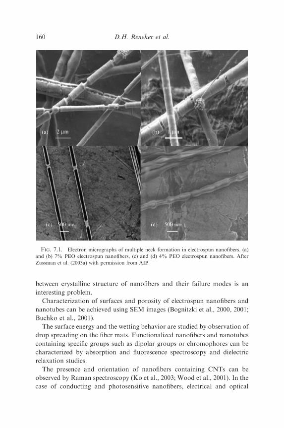
between crystalline structure of nanofibers and their failure modes is an

interesting problem.

Characterization of surfaces and porosity of electrospun nanofibers and

nanotubes can be achieved using SEM images (Bognitzki et al., 2000, 2001;

Buchko et al., 2001).

The surface energy and the wetting behavior are studied by observation of

drop spreading on the fiber mats. Functionalized nanofibers and nanotubes

containing specific groups such as dipolar groups or chromophores can be

characterized by absorption and fluorescence spectroscopy and dielectric

relaxation studies.

The presence and orientation of nanofibers containing CNTs can be

observed by Raman spectroscopy (Ko et al., 2003; Wood et al., 2001). In the

case of conducting and photosensitive nanofibers, electrical and optical

FIG. 7.1. Electron micrographs of multiple neck formation in electrospun nanofibers. (a)

and (b) 7% PEO electrospun nanofibers, (c) and (d) 4% PEO electrospun nanofibers. After

Zussman et al. (2003a) with permission from AIP.


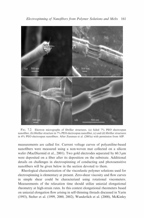
measurements are called for. Current voltage curves of polyaniline-based

nanofibers were measured using a non-woven mat collected on a silicon

wafer (MacDiarmid et al., 2001). Two gold electrodes separated by 60.3 mmwere deposited on a fiber after its deposition on the substrate. Additional

details on challenges in electrospinning of conducting and photosensitive

nanofibers will be given below in the section devoted to them.

Rheological characterization of the viscoelastic polymer solutions used for

electrospinning is elementary at present. Zero-shear viscosity and flow curves

in simple shear could be characterized using rotational viscometers.

Measurements of the relaxation time should utilize uniaxial elongational

rheometry at high-strain rates. In this context elongational rheometers based

on uniaxial elongation flow arising in self-thinning threads discussed in Yarin

(1993), Stelter et al. (1999, 2000, 2002), Wunderlich et al. (2000), McKinley

FIG. 7.2. Electron micrographs of fibrillar structures. (a) failed 7% PEO electrospun

nanofiber, (b) fibrillar structure in 7% PEO electrospun nanofiber, (c) and (d) fibrillar structures

in 4% PEO electrospun nanofibers. After Zussman et al. (2003a) with permission from AIP.


and Tripathi (2000) and Yarin et al. (2004) can be very helpful to characterize

spinnability and rheological parameters of the solutions depending on

polymer type and concentration. It is absolutely necessary to characterize

rheological behavior of the polymer solutions used in electrospinning both in

shear and elongation, since their effective viscosity actually depends on several

other basic parameters (like zero-shear viscosity and the relaxation time)

which are responsible for viscoelasticity. Such an approach was demonstrated

by Theron et al., (2004). The solutions listed in Table 7.1 were studied. Shear

viscosities of the fluids were measured at different shear rates using a Coutte

viscometer (Brookfield DV- II+programmable viscometer). Measurements

of the shear viscosity at different shear rates for different solutions of PEO

(Mw ¼ 6� 105 gmol�1) demonstrate a pronounced shear thinning, as shown

in Fig. 7.4. The values of the zero-shear viscosity m are presented in Table 7.1.

Relaxation times, y characterizing viscoelastic properties of the electrospun

solutions are also presented in Table 7.1. Relaxation times of PCL solutions

could not be measured because of the high evaporation rates of the solvents,

acetone and methylene chloride (MC). Surface tension measurements were

conducted with a pulsating bubble surfactometer. Comparison of the surface

tension of solutions of PEO (Mw ¼ 6� 105 gmol�1) in ethanol/water (40/60)

suggests that the surface tension is mainly a function of the solvent in the

solutions and tends to be less sensitive to variation in the polymer

concentration. Therefore, the values of surface tension are given in Table

7.2 as the solvent properties.

FIG. 7.3. Typical X-ray pattern of the oriented nanofiber rope made of 6% PEO

(MW ¼ 600,000 gmol�1) aqueous solution with 40% ethanol. After Zussman et al. (2003a) with



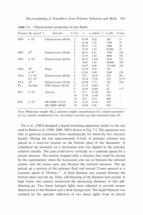
Xu et al., (2003) designed a liquid-stretching apparatus similar to the one

used in Stelter et al. (1999, 2000, 2002) shown in Fig. 7.5. The apparatus was

able to generate extensional flows mechanically for relatively low viscosity

liquids. During the test approximately 0.2mL of polymer solution was

placed in a reservoir located on the bottom plate of the rheometer. A

cylindrical tip mounted on a horizontal arm was dipped in the polymer

solution initially. The arm could move vertically at a constant speed for a

certain distance. The motion stopped after a distance that could be chosen

by the experimenter when the horizontal arm ran in between the infrared

emitter and the sensor pair and blocked the infrared emission. The tip

picked up a portion of the polymer fluid and moved 21mm upward at a

constant speed of 350mm s�1. A fluid filament was created between the

bottom plate and the tip. Then, self-thinning of the filament had started. A

high frame rate camera monitored the decreasing diameter of this self-

thinning jet. Two linear halogen lights were adjusted to provide proper

illumination to the filament and a dark background. The liquid filament was

outlined by the specular reflection of two linear lights from its lateral

Table 7.1. Characteristic properties of test fluids.

Polymer MW (gmol�1) Solvents C (%) er se (mSm�1) m (cP) y (ms)

PEO 6 105 Ethanol/water (40/60) 2 67.09 0.85 285 21

3 61.44 1.38 1200 25

4 66.57 1.15 3000 28

6 57.63 1.67 43200 33

PEO 106 Ethanol/water (40/60) 2 66.71 0.81 1590 142

3 67.97 1.28 9600 183

PEO 4 106 Ethanol/water (40/60) 1 66.12 1.102 4250 217

2 70.07 1.45 90,000 298

3 65.07 0.88 335,000 359

PEO 106 Water 2 81.96 9.43 570 –

4 106 1 110.6 8.49 2600 128

PAA 2.5 105 Ethanol/water (40/60) 6 79.5 24.47 455 48.1

4.5 105 5 74.14 17.95 255 22.75

PVA 104 Ethanol/water (50/50) 6 65.99 3.73 355 29.6

PU Tecoflex THF/ethanol (50/50) 6 16.75 0.093 25 –

8 14.45 0.069 82 1.77

PCL 8 104 Acetone 8 25.2 0.142 107 –

10 25.38 0.141 165 –

14 24.8 0.12 400 –

PCL 8 104 MC/DMF (75/25) 10 18.55 0.191 670 –

MC/DMF (40/60) 10 24.49 0.36 950 –

Note: Molecular weight (Mw), polymer weight concentration (C), relative permittiv-

ity (er), electric conductivity (s), zero-shear viscosity (m) and relaxation time (y).


surface. The contour of the filament was seen as two bright lines on a dark

background. Fig. 7.6 shows the reflections of the two linear light sources

from the lateral surface of the liquid filament.

The high-speed camera was run at 500 frames s�1. The field of view was

approximately 2mm� 2mm. A calibration procedure was carried out to

FIG. 7.4. Shear viscosity versus shear rate. Plots for solutions of PEO (MW ¼ 6 105 g/mol)

in ethanol/water (40%/60%) at different weight concentrations. After Theron et al. (2004) with

permission from Elsevier.

Table 7.2. Characteristic properties of solvents.

Solvents er se (mSm�1) Z (cP) s (mNm�1)

Distilled water 88.75 0.447 1.12 72

Ethanol (95%) 24.55* 0.0624 1.1* 22.3*

Acetone 20.7* 0.0202 0.36* 23.3*

Ethanol/water (40/60) 69.47 0.150 2.49 30y

MC/DMF (40/60) 29.82 0.505 0.93 31.6

MC/DMF (75/25) 21.3 0.273 0.73 28.9

THF/ethanol (50/50) 15.79 0.037 0.89 23.7

Note: Relative permittivity (er), electric conductivity (se), viscosity (Z) and surface

tension (s). (*) http://www.bandj.com/Home.html.

Source: Wohlfarth and Wohlfarth (1997).


correlate the distance between pixels on screen with the dimensions in real

space. Jet diameter was calculated from the distance between two contour

lines. The initial jet diameter d0 was recorded when the probe tip reached its

highest position at time t0 ¼ 0ms. Fluid jets with diameters as small as

80 mm could be accurately measured.

The whole set-up was mounted on a vibration-damped imaging bench. A

special sample fluid holder was designed to minimize filament vibration

during the thinning process. Various shapes of tips were tested. A flat-faced

tip was used to minimize the end region of the liquid filament.

The polymer concentrations were much higher than those used by Stelter

et al. (1999, 2000, 2002). In the latter works filament self-thinning was due to

surface tension, which results in the following expressions for the filament

diameter d ¼ 2a and the elongational viscosity mel

d ¼ d0expð�t=3yÞ, (7.1a)

mel ¼3ysd0

exp t=3y�

, (7.1b)

FIG. 7.5. The illustration of the fluid stretching apparatus. After Xu et al. (2003).


where s is the surface tension. Note, that the values of the relaxation time

given in Table 7.1 were obtained by fitting Eq. (7.1a) to the experimental

data.

On the contrary, concentrated polymer solutions studied by Xu et al.

(2003) thinned mostly due to gravity, which resulted in the following

expressions

d ¼ d0expð�t=2yÞ, (7.2a)

mel ¼ rgl0yexpðt=yÞ, (7.2b)

where r is the solution density, l0 the initial filament length, and g gravity

acceleration.

Fig. 7.7 shows the entire filament during stretching and self-thinning. The

cylindrical shape of the filament reflects that a uniform elongational flow

was produced. At the middle part of the filament pure extensional

deformation was created. The diameter decrease was monitored at this

position. The large strain was produced by long residence time of the

filament during the thinning process. The optical system allowed filaments

FIG. 7.6. Reflections of two linear light sources from the lateral surface of the liquid

filament (Xu, 2003).


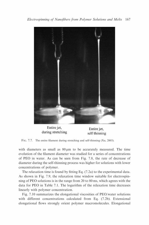
with diameters as small as 80 mm to be accurately measured. The time

evolution of the filament diameter was studied for a series of concentrations

of PEO in water. As can be seen from Fig. 7.8, the rate of decrease of

diameter during the self-thinning process was higher for solutions with lower

concentrations of polymer.

The relaxation time is found by fitting Eq. (7.2a) to the experimental data.

As shown in Fig. 7.9, the relaxation time window suitable for electrospin-

ning of PEO solutions is in the range from 20 to 80ms, which agrees with the

data for PEO in Table 7.1. The logarithm of the relaxation time decreases

linearly with polymer concentration.

Fig. 7.10 summarizes the elongational viscosities of PEO/water solutions

with different concentrations calculated from Eq. (7.2b). Extensional

elongational flows strongly orient polymer macromolecules. Elongational

FIG. 7.7. The entire filament during stretching and self-thinning (Xu, 2003).


viscosities increase during the self-thinning process. The figure also shows

that the low-concentration solution has a lower initial elongational viscosity.

However, the viscosity increases at a much faster speed, during the self-

thinning process, compared with the high-concentration solution. The fast

building up of the elongational viscosity of the low-concentration solution

corresponds to the faster diameter decrease.

0

6%

100

200

300

400

500

600

700

0 50 100 150 200 250 300 350 400 450

Dia

met

er (

mic

ron)

2% 4% 8%

10%

80

Time(ms)

FIG. 7.8. Time evolution of the liquid filament (Xu, 2003).

0 2 4 6 8 10

Concentration range

suitable for electrospinning

0.2

0.18

0.16

Rel

axat

ion

Tim

e (s

)

0.12

0.14

0.1

0.08

0.06

0.04 0.048

0.02

0

Concentration (%)

y = 0.0076e0.308x

FIG. 7.9. Relaxation time of aqueous PEO solutions (Xu, 2003).


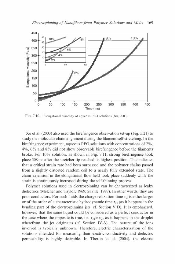
Xu et al. (2003) also used the birefringence observation set-up (Fig. 5.21) to

study the molecular chain alignment during the filament self-stretching. In the

birefringence experiment, aqueous PEO solutions with concentrations of 2%,

4%, 6% and 8% did not show observable birefringence before the filaments

broke. For 10% solution, as shown in Fig. 7.11, strong birefringence took

place 508ms after the stretcher tip reached its highest position. This indicates

that a critical strain rate had been surpassed and the polymer chains passed

from a slightly distorted random coil to a nearly fully extended state. The

chain extension in the elongational flow field took place suddenly while the

strain is continuously increased during the self-thinning process.

Polymer solutions used in electrospinning can be characterized as leaky

dielectrics (Melcher and Taylor, 1969; Saville, 1997). In other words, they are

poor conductors. For such fluids the charge relaxation time tC is either larger

or of the order of a characteristic hydrodynamic time tH (as it happens in the

bending part of the electrospinning jets, cf. Section V.D). It is emphasized,

however, that the same liquid could be considered as a perfect conductor in

the case where the opposite is true, i.e. tHbtC, as it happens in the droplet

wherefrom the jet originates (cf. Section IV.A). The nature of the ions

involved is typically unknown. Therefore, electric characterization of the

solutions intended for measuring their electric conductivity and dielectric

permeability is highly desirable. In Theron et al. (2004), the electric

6%

8% 10%

0

50

100

150

200

250

300

350

400

450

0 50 100 150 200 250 300 350 400 450

2%

4%

6%

8%10%

0

10

20

30

40

50

05 0 100

Elo

ngat

iona

l vis

cosi

ty (

Pa.

s)

2%

4%

6%

8%10%

0

10

20

30

40

50

0 50 100

Time (ms)

FIG. 7.10. Elongational viscosity of aqueous PEO solutions (Xu, 2003).


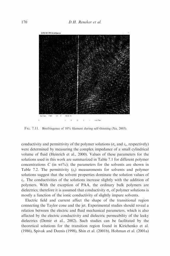
conductivity and permittivity of the polymer solutions (se and er, respectively)were determined by measuring the complex impedance of a small cylindrical

volume of fluid (Heinrich et al., 2000). Values of these parameters for the

solutions used in this work are summarized in Table 7.1 for different polymer

concentrations C (in wt%); the parameters for the solvents are shown in

Table 7.2. The permittivity (er) measurements for solvents and polymer

solutions suggest that the solvent properties dominate the solution values of

er. The conductivities of the solutions increase slightly with the addition of

polymers. With the exception of PAA, the ordinary bulk polymers are

dielectrics; therefore it is assumed that conductivity se of polymer solutions is

mostly a function of the ionic conductivity of slightly impure solvents.

Electric field and current affect the shape of the transitional region

connecting the Taylor cone and the jet. Experimental studies should reveal a

relation between the electric and fluid mechanical parameters, which is also

affected by the electric conductivity and dielectric permeability of the leaky

dielectrics (Demir et al., 2002). Such studies can be facilitated by the

theoretical solutions for the transition region found in Kirichenko et al.

(1986), Spivak and Dzenis (1998), Shin et al. (2001b), Hohman et al. (2001a)

FIG. 7.11. Birefringence of 10% filament during self-thinning (Xu, 2003).


and Feng (2002, 2003). In Theron et al. (2004) experiments on electrospinning

were performed with an apparatus shown in Fig. 7.12. The electrospun

nanofibers were collected on a large flat copper collector (400mm� 400mm).

The collector was connected to ground through a resistor. The potential drop

across the resistor was measured and translated to electric current using

Ohm’s law. The volume charge density, r, was calculated using the equation

r ¼ I/Q, where I is the electric current and Q the volumetric flow rate. The

initial surface charge density was calculated as q ¼ (rd/4)10�7 where d (mm) is

the measured diameter of the jet close to the tip of the Taylor cone, and q

(C cm�2) the surface charge density calculated at the point of the diameter

measurements. The volume charge density is a useful parameter even though

the charge is almost always on the surface of the jet. Total charge per total

volume can only change by processes that are highly improbable during

electrospinning (due to relatively low strengths of the electric field involved

and suppression of liquid atomization by the elastic forces) if airborne charges

FIG. 7.12. Sketch of the experimental setup for measuring the electric current in

electrospun jets. Nominal voltage at the source was about 10 kV, and at the syringe exit-

about 600V lower. Electrical current through the liquid was suitably small and ohmic heating

and sparking to ground were eliminated. After Theron et al. (2004) with permission from

Elsevier.


are eliminated. For the polymer solutions listed in Table 7.1 the charge

density can be described by the following expression

r ¼ kexpUpU

0 QprQ CpC MpMw e�H=hC

pCetet (7.3)

where kexp ¼ 0.012870.00556, U is the applied voltage in kV, Q is the

volumetric flow rate in mLmin�1, C is the polymer concentration in weight %,

Mw is the molecular weight of the polymer in gmol�1, H is the nozzle-

to-ground distance in cm and Cet is the ethanol concentration in weight%

(this factor should be accounted only for PEO solutions). In Eq. (7.3),

pU ¼ 3; prQ ¼ �0:8; pC ¼ 0:75; pM ¼ 0:5; pCet ¼ �0:11 (7.4)

and h in cm is given by the expression

h Mwð Þ ¼ khM MphMw , (7.5)

where khM ¼ 43:66 and phM ¼ �0:496:

VIII. Development and Applications of Several Specific Types of Nanofibers

A. BIOFUNCTIONAL (BIOACTIVE) NANOFIBERS FOR SCAFFOLDS IN TISSUE

ENGINEERING APPLICATIONS AND FOR DRUG DELIVERY AND WOUND

DRESSING

Electrospun nanofiber mats are attractive for tissue engineering mainly as

a scaffold forming a matrix for cell proliferation or for the extracellular

matrix (ECM) deposition. The matrix is, in vivo, a 3D scaffold for cells, and

provides them with a tissue with specific environment and architecture.

Furthermore, it serves as a reservoir of water, nutrients, cytokines and

growth factors (Salgado et al., 2004). Tissue engineering in vitro and in vivo

involves the interaction of cells with a material surface and with substances

that can be transported through the fibers. The nature of the surface and the

chemical constitution of the fiber can directly influence cellular response,

ultimately affecting the rate and quality of new tissue formation. Nanofibers

formed by electrospinning attract attention of the research community by

virtue of their structural similarity to natural ECM. By controlling the

electrospinning process, many essential properties of the as-spun scaffold

can be adjusted, such as the gross morphology, the microtopography, the

porosity and the chemistry of the surface. All these properties which will be

discussed herein determine which molecules can adsorb and how cells will

attach and align themselves on a scaffold.


1. Processing Techniques

Electrospinning of scaffolds for tissue engineering applications follows the

trends characteristic of electrospinning of the other polymer materials. For

scaffold applications, polymer solutions are electrospun from the tip of a

pendant or sessile drop at the edge of a syringe needle by applying electric

potential differences of the order of 10 kV, or the field strengths of the order

of 1 kV cm�1 (Boland et al., 2001; Buchko et al., 2001; Li et al., 2002).

Nanofibers are collected on a ground plate as a non-woven mat as usual, or

on a rotating mandrel as in Matthews et al. (2002). The latter introduces

slight orientation in the electrospun mats, which is beneficial for cell

attachment and growth. Kidoaki et al. (2005) developed multi-layering and

mixing methods shown in Fig. 8.1. In the multi-layering electrospinning

technique a layer-by-layer method is employed, such that a multi-layered

nanofiber mesh is created. The structure can consist of different materials

and with different porosity. In the mixing technique different polymer can

be spun simultaneously which results in a mixed scaffold. An example of a

product created by sequential multi-layering is shown in Fig. 8.1. A multi-

layered product is a tube that was produced from segmented polyurethane

SPU and collagen (see Fig. 8.2). This design is of a potential use for small-

diameter compliant artificial vascular graft.

FIG. 8.1. The electrospinning techniques for scaffold formation: (a) multi-layering and (b)

mixing. After Kidoaki et al. (2005) with permission from Elsevier.


Additional applications of the electrospun nanofiber mats as soft-tissue

prostheses were recently presented. Espy et al. (2004) used as-spun elastin

fibers in bladders tissue engineering. Boland et al. (2004) have demonstrated

the electrospinning of micro- and nano-fibrous scaffoldings from collagen

and elastin and applied these to development of biomimicking vascular

tissue-engineered constructs.

Biodegradable scaffolds can be made from poly(glycolic acid) (PGA),

poly(L-lactic acid), (PLA), poly(e-caprolactone) (PCL), and their copoly-

mers (e.g. PLGA) (e.g. Zheng et al., 2003). An example of the as-spun PCL

nanofibers is shown in Fig. 8.3. These materials have many favorable

properties, although these polymers have not performed up to the

expectation in a clinical setting (Matthews et al., 2002). That is the reason

that natural materials like collagen prepared from calfskin and from human

placenta were used to electrospin skin scaffolds (Huang et al., 2001a;

Matthews et al., 2002).

Solution drying at the nozzle exit is quite common in electrospinning of

PCL (Reneker et al., 2002) and PLA (Larsen et al., 2004). In the latter work,

coaxial solvent vapor flow was demonstrated to be capable of preventing

premature drying, solidification and clogging of the nozzle.

FIG. 8.2. Fabricated bilayered tubular construct of SPU/collagen. (1) Appearance of the

tube (scale bar 1mm). (2) SEM micrograph of the tube. (3) Magnified image of region 3 in the

photo (2). (4a–c) Magnified images of the outer layer of region 4 in the photo (2). (5a–c)

Magnified images of the inner layer of region 5 in the photo (2). After Kidoaki et al. (2005) with

permission from Elsevier.


Fang and Reneker (1997) reported producing calf thymus Na-DNA fibers

with beads structure through electrospinning from aqueous solutions with

concentration from 0.3 to 1.5%. Scanning electron micrographs showed that

the fibers had diameters as small as 30 nm and beads with diameters from 80

to 200 nm. The beads suggest that some of the DNA retracted into droplets

at intervals along the fiber. In the fiber with diameter of 62 nm about 600

DNA molecules could pass through each cross-section. Transverse striations

on the fibers, about 3–6 nm wide, were also found.

There are some indications that smooth muscle cells can better infiltrate a

slightly oriented matrix (Matthews et al., 2002). This conclusion could be

checked using fully oriented matrixes produced by the method of Theron

et al. (2001); cf. Section VI, Yang et al. (2005) and Ramakrishna et al. (2005).

This has been recently done in Xu et al. (2004), where favorable interaction of

such scaffolds with human coronary artery smooth muscle cells was

demonstrated. To the best of our knowledge, nanofibers or oriented nanofiber

ropes still have not been used for nerve regeneration. The method of Theron

et al. (2001) can easily be applied for fabrication of oriented ropes of

conducting nanofibers, which can be tested as nerve substitutes. Nanofiber

mats have great potential as scaffolds for artificial skin and artificial organs.

Electrostatic spinning was applied to the preparation of drug-laden non-

biodegradable nanofibers for potential use in topical drug administration

and wound healing. The specific aim of these studies was to assess whether

FIG. 8.3. SEM micrograph of electrospun PCL poly(e-caprolactone) nanofibers. The fiberswere spun from a 15wt.% PCL solution in DMF/DCM (25:75) with applied electrostatic field

of 1 kV/cm (Zussman et al., 2004).


these systems might be of interest as delivery systems for poorly water-

soluble drugs. Antifungal agents (itraconazole and ketanserin) were selected

as model compounds while a segmented PU was selected as the non-

biodegradable polymer (Verreck et al., 2003). For both itraconazole and

ketanserin, an amorphous nanodispersion with PU was obtained when the

drug/polymer solutions were electrospun from dimethylformamide (DMF)

and dimethylacetamide (DMAc), respectively. The collected non-woven

fabrics were shown to release the drugs at various rates and profiles based on

the nanofiber morphology and drug content. The electrospinning of

colloidal particles such as fungicides blended in polymer solutions results

in the production of nanofibers with incorporated nanoparticles. The water

insoluble polymer, PCL, was used for producing nanofibers ranging

200–1000 nm in diameter. Acetone suspensions of the fungicides Benomyl

or Ciclopirox containing the antifungal agents were added to PCL solutions

and the mixture was electrospun using electrostatic field strength of about

3 kV cm�1. Fungicide granules could be observed, by scanning electron

microscopy, to be associated with the produced nanofibers (see Fig. 8.4).

The effect of different electrospinning conditions on antifungal activity

(against Penicillium digitatum, and Sclerotinia sclerotiorum) was determined

by diffusion assays.

Electrospinning as encapsulation of various drugs inside as-spun

nanofibers was also demonstrated by Kenawy et al. (2002) and Sanders et

al. (2003). The drugs can further be released when nanofiber mats have been

implanted or attached to a human body. Prediction, measurement and

control of the release rate pose interesting unsolved applied mechanical

problems. Viruses can also be encapsulated in the electrospun nanofibers

(Lee and Belcher, 2004).

FIG. 8.4. SEM micrographs of fungicide-embedded electrospun nanofibers made from

solution of PCL 10wt.% in acetone and Circlopirox powder (Zussman et al., 2004).


2. Surface Properties

The physical and chemical characteristics of the scaffold surface mediate

the adsorption of biological molecules that regulate cell activities, such as

adhesion and migration (Boyan et al., 1996). Cells are able to attach to the

electrospun mat and proliferate into it. Therefore, design criteria of an ideal

engineering scaffold include favorable cell–matrix interactions, and bio-

compatibility of the structure (Li et al., 2002). The results of the latter work

show suitable biocompatibility for mouse fibroblasts and human bone-

marrow-derived mesenchymal stem cells on poly(D,L-lactide-co-glycolide)

(PLGA) nanofibers. This opens possibilities for scaffolding human skin,

cartilage, cardiovascular and bone-like materials. To make bones, cells

should be calcium-producing, which is an essential structural element.

The hydrophilicity (wettability) of the electrospun scaffolds is related to

the static contact angles between the scaffold and the buffer solution

containing MC3T3-E1 (mouse calvaria osteoblast) cells; Kim et al. (2003).

The contact angle of the cell-containing solution with an electrospun

scaffold made of pure PLGA, poly(lactide-co-glycolide) (LA/GA ¼ 75/25,

Mw ¼ 75,000) was 1051. The contact angle value between purified water and

the same electrospun mat was also 1051. That suggested that the presence of

the cells did not alter wettability of this electrospun mat.

The feasibility of obtaining a hydrophobic electrospun mat from high-

molecular weight polymer was demonstrated by Deitzel et al. (2002). They

electrospun polymer blends composed of PMMA with a varying amount of

tetrahydroperfluorooctyl acrylate (TAN) with the concentration of TAN in

the range from 0 to 10%. The fiber diameters were in the range from 0.1 to

2 mm. Beads, due to capillary instability, were observed along the fibers.

Jiang et al. (2004) demonstrated that an electrospun mat fabricated from a

25wt% solution of polystyrene PS in DMF created a superhydrophobic

surface with water, with a contact angle of 160.41. This work resulted in

nanofibers, which create a mat with two scales, the fiber scale and the beads

scale. Such morphology reveals superhydrophobic behavior as in the famous

lotus effect.

To tackle the hydrophobic properties of polymer mats which are normally

resistant to infiltration of water into their pores, a surface treatment with

ethanol was suggested (Stitzel et al., 2001). The treatment was demonstrated

on an electrospun PLA mat, which was wetted by immersion in ethanol

followed by immersion in water. In particular, the mat was wetted with 100%

ethanol for 30min, rinsed once with sterile water and placed in fresh sterile

water for 30min. The wetting procedure allows an effective penetration of


cells into the interstices of the matrix, as well as simultaneously sterilizing the

matrix/fiber structure.

3. Porosity

Porosity and interconnectivity are essential in scaffolds for diffusion of

nutrients and gasses and/or for removal of metabolic waste (Salgado et al.,

2004). Scaffolds must posses open pores and a fully inter-connected geometry in

a highly porous structure with a large surface area to volume ratio. That will

aid migration of growing cells throughout the porous structure. Furthermore,

the scaffolds should also exhibit adequate microporosity in order to allow

capillary ingrowth. Pore sizes and flexibility are also very important.

An electrospun nanofiber mat of copolymer PLGA [85:15; PL:GA]

resulted in porosity of 91.63%. The pore diameter distribution measured by

a mercury porosimeter indicated that pore diameter ranged broadly from 2

to 465 mm. The effective pore diameters for cell ingrowth into a non-woven

mat are between 20 and 60 mm while for bone ingrowth 75–150 mm are

required (Li et al., 2002). If in a non-woven mat of nanofibers the fibers are

not attached at contact points, cells are able to push nanofibers aside.

Therefore, even the smallest pores could become appropriate for cell

ingrowth. Salgado et al. (2004) argue that for bone tissue engineering

purposes, pore size should be within the 200–900 mm range. Holy et al.

(2000) reported an application of electrospinning for bone tissue engineering

where they investigated a scaffold made of biodegradable PLGA 75/25. The

scaffold exhibited a regular distribution of inter-connected macropores with

diameters in the range from 1.5 to 2.2mm.

4. Mechanical Properties

The strength and elasticity of a scaffold are other important aspects for its

design. The scaffold should withstand the expected mechanical stresses and

ideally match the mechanical behavior of its immediate environment. In

bone tissue engineering, because the bone is subjected to varying stress, the

mechanical properties of the implanted construct should ideally match those

of the living bone (Hutmacher, 2000). Zong et al. (2003) showed that

electrospun PLGA membranes are promising scaffolds for applications such

as regeneration of heart tissue. Cardiac myocytes were found to remodel the

flexible electrospun matrix by pulling on fibers and moving into the scaffold

to form dense multiple layers.


Stress–strain curves measured for polymer nanofiber mats of interest in

the tissue engineering field, PGA and PLGA revealed mechanical properties

of their non-woven mats comparable to those of human cartilage and skin.

The tensile (Young’s) modulus E was of the order of 300MPa, the ultimate

(maximal) tensile stress was about 23MPa and the strain at breakup was

about 96% (Boland et al., 2001; Li et al., 2002). For non-woven mats of

poly(e-caprolactone), PCL, the ultimate tensile stress and strain were found

to be of about 1–2MPa and 200%, respectively (Lee et al., 2003a). The

Young’s modulus was of the order of 3–5MPa, and the yield stress was

0.5–0.6MPa (Lee et al., 2003a). Measurements done for quasi-parallel fiber

mats of polylactide, PLA, using 250–1000 nm nanofibers, revealed an

ultimate tensile stress of about 0.1MPa and an ultimate tensile strain of

about 14% (Dersh et al., 2003).

B. CONDUCTING NANOFIBERS: DISPLAYS, LIGHTING DEVICES, OPTICAL

SENSORS, THERMOVOLTAIC APPLICATIONS

Electrospinning of conducting nanofibers was considered briefly in

Section VI. In the present section, we extend the discussion. Poly(pyrrole),

polyaniline, PEDOT, PPV and MEH-PPV (poly(2-methoxy, 5-(20-ethyl-

hexoxy)-p-phenylenevinylene) are the conducting conjugated polymers

which received the most attention from the researchers dealing with fiber

and nanofiber applications. The interest is related first of all to their possible

applications in micro- and opto-electronics. LEDs made of conjugated

polymers have been examined for such applications as displays and lighting

(Weder et al., 1998; Ho et al., 1999). The intrinsic anisotropy of the

electronic structure of such molecules means that provided they can be

oriented into a specific direction, emission of polarized light will occur. A

polarization ratio 200:1 would not require power inefficient external

polarizers to produce useful polarized light (Whitehead et al., 2000). In

order to optimize the broad range of the electrical properties of conjugated

polymers, a variety of processing techniques were developed to improve the

structural order to the point that the intrinsic properties of the

macromolecular chains can be achieved. These techniques include mechan-

ical alignment by rubbing, stretching (Grell and Bradley, 1999) or alignment

of luminescent ‘‘guest’’ molecules in a ‘‘host’’ polymer matrix (Hagler et al.,

1991). Further improvement in material quality is expected in the intrinsic

electronic properties of conjugated polymers, as well as improvement of the

ability to fabricate thin media for creating power efficient devices that

operate at low voltage.


Srinivasan and Reneker (Srinivasan, 1994) reported electrospun polyani-

line (VERSICONs) fibers from solutions in concentrated sulfuric acid

(95–98%) containing 15–18% by weight of the polymer. The electrospun

fibers were green in color in the conducting state. They were often curved

and looped. Roughness of the surface of the fibers measured with an STM

on a 100� 100 nm2 area was about 18. The diameter of the polyaniline fibers

ranges from about 40 nm to about a micron. These diameters are the lowest

reported for polyaniline. Such fibers can potentially be used in electro-

mechanical actuators, which convert electrical energy to mechanical energy

using doping/dedoping or charge transfer reactions that cause large

dimensional changes in the system. Srinivasan and Reneker proved by the

successful imaging of the surface of the fibers using an STM that the fibers

were electrically conducting.

Electrospinning represents a very promising technique for fabrication of

luminescent nanofibers based on conducting, photosensitive polymers. The

high value of the area reduction ratio and the associated high longitudinal

strain rate (�1000 s�1) imply that macromolecules in the nanofibers should

be elongated and oriented in the direction of the jet axis. In the present

context, the aim is to electrospin spinnable ‘‘host’’ polymer nanofibers

containing light-emitting ‘‘guest’’ conjugated polymers, and conjugated

polymers are typically not spinnable. Utilizing the high degree of chain

extension, chain alignment and structural order attainable, in principle, in

electrospinning of the ‘‘host’’ polymer, one can expect to induce a similar

order in the ‘‘guest’’ conjugated macromolecules incorporated in the

nanofiber. This will allow a combination of the mechanical properties of

electrospun ‘‘host’’ polymer nanofiber with the electric conductivity and the

anisotropic linear and non-linear optical properties of the conjugated

‘‘guest’’ polymer.

Electrospinning of a blend of polyaniline doped with camphorsulfonic

acid (PAn.HCSA) and PEO was previously demonstrated (MacDiarmid

et al., 2001; Norris et al., 2000; MacDiarmid, 2001). The electrospun

nanofibers had diameters ranging between 950 and 2100 nm, with a

generally uniform thickness along the fiber. The fibers formed a non-woven

mat with high porosity and a relatively low conductivity compared to cast

films. The method proposed in Theron et al. (2001) and Zussman et al.

(2003b) allows assembly of the individual electrospun nanofibers aligned

with a preferable orientation relative to the substrate, as well as nanofiber

crossbars. In this method, both high molecular orientation of the nanofibers

and a structural orientation are guaranteed. Photovoltaic diodes, which

could be based on such nanofibers, are described in Granstrom et al. (1998).


Teye-Mensah et al. (2004) and Tomer et al. (2005) reported erbium (III)

oxide particles hybrided with titania nanofibers electrospun from mixed

solution of tetraisopropyl titanate (TPT) and polyvinylpyrrolidone (PVP);

Fig. 8.5. The electrospun nanofibers were thermally annealled at 900oC to

pyrolyse the PVP, leaving nanofibres of rutile-phase titania. The erbium (III)

oxide particles modify the near-infrared optical properties of the titania

nanofibres as are verified both by absorption and emission spectra. They

demonstrated that the diameters of the nanofibers can be controlled by

adjusting the precursor solution, and the crystal structure can be adjusted by

annealing at different temperatures. Temperature-dependent near-infrared

emission spectra demonstrate that the erbia-containing nanofibers emit

selectively in the range 6000–7000 cm�1. These high-temperature optically

functionalized nanostructures with large surface to volume ratios and

narrow-band optical emission can be used in a thermophotovoltaic energy

conversion system.

C. PROTECTIVE CLOTHING, CHEMICAL AND BIOSENSORS AND SMART

FABRICS

Protective clothing is expected to employ polymer nanofibers as a key

element (Schreuder-Gibson et al., 2002, 2003). The advantages of using

nanofibers in protective clothing are twofold: (i) Nanofiber mats have a huge

internal surface, which allows an enhanced contact area between the protective

medium and dangerous and aggressive environment. Examples of such an

environment are lethal gases such as mustard gas, sarin and nerve gases, as well

FIG. 8.5. Scanning electron microscope images of self-supporting and continuous titania

nanofibers after pyrolysis. These structures result from electrospinning TPT/PVP solutions with

ratios of (a) 0.2 and (b) 0.4 by weight. The scale bar in both panels is 1mm. After Teye-Mensah

et al. (2004) with permission from IOP.


as aerosols of contagious disease spores, which could be used in chemical and

biological warfare. (ii) It is relatively easy to incorporate different chemical

agents into polymer solutions and, via electrospinning, into polymer nanofibers.

These agents could effectively deactivate dangerous chemical and biological

compounds in contact with them, and thus protect personnel. Nanofibers

containing deactivating agents can also be used in gas masks. For all these

applications, as well as for such applications as nanofiber-based filters, mass

production of nanofibers at fast rate becomes crucial. This both makes scale-up

of the manufacturing process based on electrospinning and the search for

appropriate stable deactivating agents compatible with nanofiber-forming

polymer solutions important activities.

Bulletproof vests incorporating nanofibers could become more effective

and stronger than the ordinary Kevlar-based ones given the fact that spider

dragline silk is stronger than Kevlar and stretches better than nylon (cf.

Section VIII.A).

Srinivasan and Reneker (Srinivasan, 1994) reported electrospun KEV-

LARs fibers from solutions in concentrated sulfuric acid (95–98%)

containing 2–3% by weight of the polymer, PPTA. Small diameter fibers

ranging from 40 nm to a few hundreds of nanometers were successfully spun

by the electrospinning technique. These fibers were at least one order of

magnitude smaller in diameter than available textile fibers. The PPTA

molecules were shown to be oriented along the fiber axis. The electron

diffraction patterns obtained from the PPTA fibers were similar to the

electron diffraction patterns obtained from fibers spun commercially from

the liquid crystalline state. The annealing allowed the crystallites to

rearrange themselves to a more thermodynamically stable state as opposed

to a more kinetically determined arrangement in as-spun fibers. Although

PPTA is a rod-like polymer, solutions of PPTA in this process have enough

extensional flow to orient the chain molecules. Dark-field imaging revealed

crystallites whose size and orientation was characterized. High magnifica-

tion bright field images of an annealed fiber revealed alternate bright and

dark stripes suggesting the stacking of coin-shaped layers with slightly

different orientation along the fiber axis.

The tensile modules and the strength of polymers depend on the degree of

chain orientation. Achievement of a high degree of chain orientation is an

ongoing goal in the technology of high-performance polymer fibers. The

high draw ratios achieved in electrospinning (of the order of 1000) offer an

opportunity to obtain novel highly oriented nanofibers with fully extended

polymer chain conformation without recourse to rigid or ultra-long chain

architecture (cf. e.g., Kahol and Pinto, 2002).


In the work of Zussman et al. (2002), micro-aerodynamic decelerators based

on air permeable nanofiber mats were studied. The nanofibers were obtained

via electrospinning of polymer solutions. The mats were electrospun directly

onto light pyramid-shaped frames. These platforms were released and fell freely

through the stagnant air, apex down, at a constant velocity. The motivation of

Zussman et al. (2002) stems from a necessity to develop very light air-borne

platforms of weight less than 1g, capable of carrying relatively large payloads

up to several grams. The platforms should be capable of delivering various

chemical, biological, thermal and radioactivity sensors to the locations

otherwise difficult to reach. This is of crucial importance in the cases of

spillage or other dissemination of hazardous materials, and for atmospheric

studies. In spite of the fact that different platform configurations could be

imagined, their feasibility is rooted in the same question: whether or not a

permeable and thus very light parachute could possess the same drag as the

corresponding impermeable one? It was demonstrated in Zussman et al. (2002)

that terminal velocity of such permeable structures is of the order of

30–50 cms�1 with payloads of up to several grams. The reduced settling

velocity of the mats with porosities of the order of 0.8–0.9 shows that

permeable wings or parachutes based on nanofibers are feasible. Passive

platforms similar to those of the above-mentioned work would be easily

transported by wind to large distances. Active flapping or jet-propulsion-based

light flying objects fabricated via electrospinning are also possible (Pawlowski

et al., 2003). The inter-fiber spaces constitute a significant part of their area.

This fact allows for a significant reduction in the weight of these structures

compared to the corresponding impermeable structures. Permeable non-woven

nanofiber networks are sufficiently strong and have negligible weight even

compared to the light frames or to light plastic wrap. Therefore, the role of the

non-woven fiber mats attached at the frames is twofold: (i) to generate drag

force, while (ii) to reduce the weight. The ultimate aim of such a construction is

to reduce the terminal settling velocity while carrying a useful payload (e.g. a

sensor). The nanofiber mats for this purpose may ultimately be electrospun

from photo-sensitive polymers, which can generate electric power for sensors

from the sunlight, thus making the wings also a source of energy for the sensors

and their transmitters (cf. Teye-Mensah et al., 2004; Tomer et al., 2005).

Different chemical and biological indicators can easily be incorporated in

polymers. As a continuation of the work in Zussman et al. (2002), one of the

chemical indicators, bromophenol, was incorporated into nanofibers-based

airborne platforms (WMD Sensitive, 2004). It was shown that the platforms

changed their color when subjected to an appropriate acidic or basic

environment thus serving as chemical indicators. In Wang et al. (2002),


non-woven nanofiber mats containing pyrene methanol were used as a

highly sensitive fluorescence-based optical sensor for detection of explosives.

Acknowledgment

Support for this work was provided by the National Science Foundation

under Grants Nos. DMI-9813098 and CTS-9900949, by the U.S. Army

Research Office MURI Grant No. 95-0950-01-06, by the U.S. Army Soldier

and Biological Systems Command, by the Nonmetallic Materials Division

of the U.S. Air Force Research Laboratory, Wright Patterson Air Force

Base, by the GIF-German-Israeli Foundation for Scientific Research and

Development under Grant No. I-536-097.14/97, by the Israel Academy of

Sciences under Grants No. 287/00-1 and 26/03, and by a Grant from

VolkswagenStiftung, Germany. The authors gratefully acknowledge their

research collaboration with Y. Cohen, Y. Dror, H. Fong, W. Kataphinan,

R. Khalfin, S. Koombhongse, S.N. Reznik, W. Salalha and A. Theron.

References

Aref, H., and Flinchem, E. P. (1984). Dynamics of a vortex filament in a shear flow. J. Fluid

Mech. 148, 477–497.

Arms, R. J., and Hama, F. R. (1965). Localized-induction concept on a curved vortex and

motion of an elliptic vortex ring. Phys. Fluids 8, 533–559.

Bandyopadhyaya, R., Nativ-Roth, E., Regev, O., and Yerushalmi-Rozen, R. (2002).

Stabilization of individual carbon nanotubes in aqueous solutions. Nano Letters 2, 25–28.

Batchelor, G. K. (1967). An Introduction to Fluid Dynamics. Cambridge University Press,

Cambridge.

Bates, W. D., Barnes, C. P., Ounaies, Z., and Wnek, G. E. (2003). Electrostatic processing of

PVDF. Polym. Preprints, 44, 114–114.

Baumgarten, P. K. (1971). Electrostatic spinning of acrylic microfibers. J. Colloid. Interface Sci.

36, 71–79.

Bird, R. B., Armstrong, R. C., and Hassager, O. (1987). Dynamics of Polymeric Liquids, 2nd ed.

Wiley, New York.

Bognitzki, M., Czado, W., Freze, T., Schaper, A., Hellwig, M., Steinhart, M., Greiner, A., and

Wendorff, J. H. (2001). Nanostructured fibers via electrospinning. Adv. Mat. 13, 70–72.

Bognitzki, M., Hou, H., Ishaque, M., Frese, T., Hellwig, M., Schwarte, C., Schaper, A.,

Wendorff, J. H., and Greiner, A. (2000). Polymer, metal and hybrid nano- and mesotubes

by coating degradable polymer template fibers (TUFT process). Adv. Mat. 12, 637–640.

Boland, E. D., Matthews, J. A., Pawlowski, K. J., Simpson, D. G., Wnek, G. E., and Bowlin, G. L.

(2004). Electrospinning collagen and elastin: preliminary vascular tissue engineering. Front.

Biosci. 9, 1422–1432.

Boland, E. D., Wnek, G. E., Simpson, D. G., Pawlowski, K. J., and Bowlin, G. L. (2001).

Tayloring tissue engineering scaffolds using electrostatic processing techniques: a study of

poly(glycolic acid) electrospinning. J. Macromol. Sci. – Pure Appl. Chem. A38, 1231–1243.


Boyan, B. D., Hummert, T. W., Dean, D. D., and Schwartz, Z. (1996). Role of material surfaces

in regulating bone and cartilage cell response. Biomaterials 17, 137–146.

Braun, E., Eichen, Y., Sivan, U., and Ben-Yoseph, G. (1998). DNA-templated assembly and

electrode attachment of a conducting silver wire. Nature 391, 775–778.

Buchko, C. J., Kozloff, K. M., and Martin, D. C. (2001). Surface characterization of porous,

biocompatible protein polymer thin films. Biomaterials 22, 1289–1300.

Busscher, H. J., van Pelt, A. W. J., de Boer, P., de Jong, H. P., and Arends, J. (1984). The effect

of surface roughening of polymers on measured contact angles of liquids. Colloid. Surface.

9, 319–331.

Caruso, R. A., Schattka, J. H., and Greiner, A. (2001). Titanium dioxide tubes from sol–

gel coating of electrospun polymer fibers. Adv. Mat. 13, 1577–1579.

Chang, H., and Lodge, A. S. (1972). Comparison of rubberlike-liquid theory with stress-growth

data for elongation of a low-density branched polyethylene melt. Rheol. Acta 11,

127–129.

Cheng, K. J., and Miksis, M. J. (1989). Shape and stability of a drop on a conducting plane in

an electric field. Physicochem. Hydrodyn. 11, 9–20.

Cherney, L. T. (1999a). Structure of Taylor cone-jets: limit of low flow rates. J. Fluid Mech. 378,

167–196.

Cherney, L. T. (1999b). Electrohydrodynamics of electrified liquid menisci and emitted jets.

J. Aerosol Sci. 30, 851–862.

Ciferri, A., and Ward, I. M., eds. (1979). Ultra-High Modulus Polymers. Applied Science

Publishers, London.

Cobden, D. H. (2001). Molecular electronics – nanowires begin to shine. Nature 409, 32–33.

Cuenot, S., Demoustier-Champagne, S., and Nysten, B. (2000). Elastic modulus of polypyrrole

nanotubes. Phys. Rev. Lett. 85, 1690–1693.

Dalton, A. B., Blau, W. J., Chambers, G., Coleman, J. N., Henderson, K., Lefrant, S.,

McCarthy, B., Stephan, C., and Byrne, H. J. (2001). A functional conjugated polymer to

process, purify and selectively interact with single wall carbon nanotubes. Synth. Met. 121,

1217–1218.

de Gennes, P. G. (1974). Coil-stretch transition of dilute flexible polymers under ultrahigh

velocity gradients. J. Chem. Phys. 60, 5030–5042.

Deitzel, J. M., Kleinmeyer, J. D., Hirvonen, J. K., and Tan, N. C. B. (2001). Controlled

deposition of electrospun poly(ethylene oxide) fibers. Polymer 42, 8163–8170.

Deitzel, J. M., Kosik, W., McKnight, S. H., Tan, N. C. B., DeSimone, J. M., and Crette, S.

(2002). Electrospinning of polymer nanofibers with specific surface chemistry. Polymer 43,

1025–1029.

Demir, M. M., Yilgor, I., Yilgor, E., and Erman, B. (2002). Electrospinning of polyurethane

fibers. Polymer 43, 3303–3309.

Demoustier-Champagne, S., Duchet, J., and Legras, R. (1999). Chemical and electrochemical

synthesis of polypyrrole nanotubes. Synth. Met. 101, 20–21.

Dersh, R., Liu, T., Schaper, A. K., Greiner, A., and Wendorff, J. H. (2003). Electrospun

nanofibers: internal structure and intrinsic orientation. J. Polym. Sci., Polym. Chem. Ed.

A41, 545–553.

Doshi, J., and Reneker, D. H. (1995). Electrospinning process and applications of electrospun

fibers. J. Electrostat. 35, 151–160.

Drew, C., Wang, X. Y., Senecal, K., Schreuder-Gibson, H., He, J. N., Kumar, J., and

Samuelson, L. A. (2002). Electrospun photovoltaic cells. J. Macromol. Sci. – Pure Appl.

Chem. A39, 1085–1094.

Driesel, W., Dietzsch, Ch., and Muhle, R. (1996). In situ observation of the tip shape of AuGe

liquid alloy ion sources using a high voltage transmission electron microscope. J. Vac. Sci.

Technol. B14, 3367–3380.


Dror, Y., Salalha, W., Khalfin, R., Cohen, Y., Yarin, A. L., and Zussman, E. (2003). Carbon

nanotubes embedded in oriented polymer nanofibers by electrospinning. Langmuir 19,

7012–7020.

Duan, X., Huang, Y., Cui, Y., Wang, J., and Lieber, C. M. (2001). Indium phosphide nanowires

as building blocks for nanoscale electronic and optoelectronic devices. Nature 409, 66–69.

Duft, D., Achtzehn, T., Muller, R., Huber, B. A., and Leisner, T. (2003). Rayleigh jets from

levitated microdroplets. Nature 421, 128–128.

Dzenis, Y. (2004). Spinning continuous fibers for nanotechnology. Science 304, 1917–1919.

Dzhaugashtin, K. E., and Yarin, A. L. (1977). Numerical simulation of nonself-similar wall jet.

J. Eng. Phys. 32, 420–426.

Edelman, F. T. (1999). Fullerene pipes, tube-in-tube membranes, and carbon-nanotube tips:

adding new dimensions to molecular technology. Angew. Chemie – Int. Ed. 38, 1381–1387.

Entov, V. M., and Yarin, A. L. (1984). The dynamics of thin liquid jets in air. J. Fluid Mech.

140, 91–111.

Espy, P. G., McManus, M. C., Bowlin, G. L., and Koo, H. P. (2004). Electrospun elastin

scaffolds for use in bladder tissue engineering. J. Urol. 171, 457–457.

Evans, E., Brownman, H., Leung, A., Needham, D., and Tirrell, D. (1996). Biomembrane

templates for nanoscale conduits and networks. Science 273, 933–935.

Fang, Q., Chetwynd, D. G., and Gardner, J. W. (2001). Tensile properties of conducting

polymer fibres. Proc. of 2nd EUSPEN Internat. Conf., Turin, Italy 27–31(May), 32–35.

Fang, X., and Reneker, D. H. (1997). DNA fibers by electrospinning. J. Macromol. Sci. Phys.

Ed. B36, 169–173.

Feng, J. J. (2002). The stretching of an electrified non-Newtonian jet: a model for

electrospinning. Phys. Fluids 14, 3912–3926.

Feng, J. J. (2003). Stretching of a straight electrically charged viscoelastic jet. J. Non-Newtonian

Fluid Mech. 116, 55–70.

Fernandez de la Mora, J. (1992). The effect of charge emission from electrified liquid cones.

J. Fluid Mech. 243, 561–574.

Fong, H., Chung, I., and Reneker, D. H. (1999). Beaded nanofibers formed during

electrospinning. Polymer 40, 4585–4592.

Fong, H., and Reneker, D. H. (1999). Elastomeric nanofibers of styrene–butadiene–styrene

triblock copolymer. J. Polym. Sci., Polym. Phys. Ed. 37, 3488–3493.

Fong, H., and Reneker, D. H. (2000). Electrospinning and formation of nanofibers. In Structure

Formation in Polymeric Fibers (D. R., Salem, and M. V., Sussman, eds.), pp. 225–246.

Hanser, Munich.

Formhals, A. (1934). Process and apparatus for preparing artificial threads. U.S. Patent No.

1,975,504.

Frenot, A., and Chronakis, I. S. (2003). Polymer nanofibers assembled by electrospinning. Curr.

Opinion Colloid Interface Sci. 8, 64–75.

Fridrikh, S. V., Yu, J. H., Brenner, M. P., and Rutledge, G. C. (2003). Controlling the fiber

diameter during electrospinning. Phys. Rev. Lett. 90 Art. No. 144502.

Ganan-Calvo, A. M. (1997a). On the theory of electrohydrodynamically driven capillary jets.

J. Fluid Mech. 335, 165–188.

Ganan-Calvo, A. M. (1997b). Cone-jet analytical extension of Taylor’s electrostatic solution

and the asymptotic universal scaling laws in electrospraying. Phys. Rev. Lett. 79, 217–220.

Ganan-Calvo, A. M. (1999). The surface charge in electrospraying: its nature and its universal

scaling laws. J. Aerosol Sci. 30, 863–872.

Ge, J. J., Hou, H. Q., Li, Q., Graham, M. J., Greiner, A., Reneker, D. H., Harris, F. W., and

Cheng, S. Z. D. (2004). Assembly of well-aligned multiwalled nanotubes in confined

polyacrylonitrile environments. Electrospun composite nanofiber sheets. J. Am. Chem. Soc.

126, 15754–15761.


Ghadiri, M., Granja, J. R., and Buechler, L. (1994). Artificial transmembrane ion channels from

self-assembling peptide nanotubes. Nature 369, 301–304.

Granstrom, M., Petritsch, K., Arias, A. C., Lux, A., Andersson, M. R., and Friend, R. H.

(1998). Laminated fabrication of polymeric photovoltaic diodes. Nature 395, 257–260.

Grell, M., and Bradley, D. D. C. (1999). Polarized luminescence from oriented molecular

materials. Adv. Mat. 11, 895–905.

Gu, S. Y., Wu, Q. L., Ren, J., and Vansco, G. J. (2005). Mechanical properties of a single

electrospun fiber and its structures. Macromol. Rapid Commun. 26, 716–720.

Gupta, P., and Wilkes, G. L. (2003). Some investigations on the fiber formation by utilizing a

side-by-side bicomponent electrospinning approach. Polymer 44, 6353–6359.

Hagler, T. W., Pakbaz, K., Voss, K. F., and Heeger, A. J. (1991). Enhanced order and electronic

delocalization in conjugated polymers oriented by gel processing in polyethylene. Phys.

Rev. B 44, 8652–8666.

Hamley, I. W. (2000). Introduction to Soft Matter. Wiley, Chichester.

Harris, C. E., Starnes Jr., J. H. & Stuart, M. J. (2001). NATA/TM-2001-210844, April 2001.

Harris, M. T., and Basaran, O. A. (1993). Capillary electrohydrostatics of conducting drops

hanging from a nozzle in an electric field. J. Colloid Interface Sci. 161, 389–413.

Hatzor, A., and Weiss, P. S. (2001). Molecular rulers for scaling down nanostructures. Science

291, 1019–1020.

Hayati, I. (1992). Eddies inside a liquid cone stressed by interfacial electrical shear. Colloid.

Surf. 65, 77–84.

Heinrich, R., Bonisch, S., Pommerenke, D., Jobava, R., & Kalkner, W. (2000). Broadband

measurement of the conductivity and the permittivity of semiconducting materials in high

voltage XLPE cables. 8th Int. Conf. Dielect. Mater. Meas. Appl. Edinburgh, IEE Conf. Publ.

No. 473, 212–217.

Higuera, F. J. (2003). Flow rate and electric current emitted by a Taylor cone. J. Fluid Mech.

484, 303–327.

Ho, P. K. H., Thomas, D. S., Friend, R. H., and Tessler, N. (1999). All-polymer optoelectronic

devices. Science 285, 233–236.

Hohman, M. M., Shin, M., Rutledge, G., and Brenner, M. P. (2001a). Electrospinning and

electrically forced jets: I. Stability theory. Phys. Fluids 13, 2201–2220.

Hohman, M. M., Shin, M., Rutledge, G., and Brenner, M. P. (2001b). Electrospinning and

electrically forced jets: II. Applications. Phys. Fluids 13, 2221–2236.

Holy, C. E., Schoichet, M. S., and Davies, J. E. (2000). Engineering three-dimensional bone

tissue in vitro using biodegradable scaffolds: investigating initial cell-seeding density and

culture period. J. Biomed. Mater. Res. 51, 376–382.

Hou, H., and Reneker, D. H. (2004). Carbon nanotube on carbon nanofibers: a novel structure

based on electrospun nanofibers. Adv. Mat. 16, 69–73.

Hsu, C. H., Shih, H., Subramoney, S., and Epstein, A. J. (1999). High tenacity, high modulus

conducting polyaniline composite fibers. Synth. Met. 101, 677–680.

Huang, L., Apkarian, R. P., and Chaikof, E. L. (2001a). High-resolution analysis of engineered

type I collagen nanofibers by electron microscopy. Scanning 23, 372–375.

Huang, Y., Duan, X. F., Wei, Q. Q., and Lieber, C. M. (2001b). Directed assembly of one-

dimensional nanostructures into functional networks. Science 291, 630–633.

Huang, Z. M., Zhang, Y. Z., Kotaki, M., and Ramakrishna, S. (2003). A review on polymer

nanofibers by electrospinning and their applications in nanocomposites. Composite Sci.

Technol. 63, 2223–2253.

Huang, Z. M., Zhang, Y. Z., Ramakrishna, S., and Lim, C. T. (2004). Electrospinning and

mechanical characterization of gelatin nanofibers. Polymer 45, 5361–5368.

Hutmacher, D. W. (2000). Scaffolds in tissue engineering bone and cartilage. Biomaterials 21,

2529–2543.


Iijima, S. (1991). Helical microtubules of graphitic carbon. Nature 354, 56–58.

Inai, R., Kotaki, M., and Ramakrishna, S. (2005). Structure and properties of electrospun

PLLA single nanofibers. Nanotechnology 16, 208–213.

Jaeger, R., Schonherr, H., and Vancso, G. J. (1996). Chain packing in electrospun poly(ethylene

oxide) visualized by atomic force microscopy. Macromolecules 29, 7634–7636.

Jeans, J. (1958). The Mathematical Theory of Electricity and Magnetism. Cambridge University

Press, Cambridge.

Jerome, C., Labaye, D., Bodart, I., and Jerome, R. (1999). Electrosynthesis of polyacrylic

polypyrrole composites: formation of polypyrrole wires. Synth. Met. 101, 3–4.

Jiang, L., Zhao, Y., and Zhai, J. (2004). A lotus-leaf-like superhydrophobic surface: a porous

micropshere/nanofiber composite film prepared by electrohydrodynamics. Angew. Chem.-

Int. Ed. 43, 4338–4341.

Kahol, P. K., and Pinto, N. J. (2002). Electron paramagnetic resonance investigations of

electrospun polyaniline fibers. Solid State Commun. 124, 195–197.

Kedem, S., Schmidt, J., Paz, Y., and Cohen, Y. (2005). Composite polymer nanofibers with

carbon nanotubes and titanium dioxide particles. Langmuir 21, 5600–5604.

Kenawy, E. R., Bowling, G. L., Mansfield, K., Layman, J., Simpson, D. G., Sanders, E. H., and

Wnek, G. E. (2002). Release of tetracycline hydrochloride from electrospun poly(ethylene-

co-vinylacetate), poly(lactic acid), and a blend. J. Contr. Release 81, 57–64.

Khakhar, D. V., and Ottino, J. M. (1987). Breakup of liquid threads in linear flows. Int.

J. Multiphase Flow 13, 71–86.

Khil, M. S., Kim, H. Y., Kim, M. S., Park, S. Y., and Lee, D. R. (2004). Nanofibrous mats of

poly(trimethylene terephthalate) via electrospinning. Polymer 45, 295–301.

Kidoaki, S., Kwon, I. K., and Matsuda, T. (2005). Mesoscopic spatial designs of nano- and

microfiber meshes for tissue-engineering matrix and scaffold based on newly devised

multilayering and mixing electrospinning techniques. Biomaterials 26, 37–46.

Kim, B. C., Nair, S., Kim, J., Kwak, J. H., Grate, J. W., Kim, S. H., and Gu, M. B. (2005a).

Preparation of biocatalytic nanofibres with high activity and stability via enzyme aggregate

coating on polymer nanofibres. Nanotechnology 16, S382–S388.

Kim, G. M., Lach, R., Michler, G. H., and Chang, Y. W. (2005b). The mechanical deformation

process of electrospun polymer nanocomposite fibers. Macromol. Rapid Commun. 26, 728–733.

Kim, J. S., and Reneker, D. H. (1999). Mechanical properties of composites using ultrafine

electrospun fibers. Polym. Composite. 20, 124–131.

Kim, K., Yu, M., Zong, X., Chiu, J., Fang, D., Seo, Y. S., Hsiao, B. S., Chu, B., and

Hadjiargyrou, M. (2003). Control of degradation rate and hydrophilicity in electrospun non-

woven poly(D,L-lactide) nanofibers scaffolds for biomedical applications. Biomaterials 24,

4977–4985.

Kirichenko, V. M., Petrianov-Sokolov, I. V., Suprun, N. N., and Shutov, A. A. (1986).

Asymptotic radius of a slightly conducting liquid jet in an electric field. Sov. Phys. Dokl. 31,

611–614.

Ko, F., Gogotsi, Y., Ali, A., Naguib, N., Ye, H. H., Yang, G. L., Li, C., and Willis, P. (2003).

Electrospinning of continuous carbon nanotube-filled nanofiber yarns. Adv. Mat. 15,

1161–1165.

Koombhongse, S., Liu, W., and Reneker, D. H. (2001). Flat polymer ribbons and other shapes

by electrospinning. J. Polym. Sci., Polym. Phys. Ed. 39, 2598–2606.

Larrondo, L., and Manley, R. S. J. (1981a). Electrostatic fiber spinning from polymer melts.

I. Experimental observations on fiber formation and properties. J. Polym. Sci., Polym.

Phys. Ed. 19, 909–920.

Larrondo, L., and Manley, R. S. J. (1981b). Electrostatic fiber spinning from polymer melts.

II. Examination of the flow field in an electrically driven jet. J. Polym. Sci., Polym. Phys.

Ed. 19, 921–932.


Larrondo, L., and Manley, R. S. J. (1981c). Electrostatic fiber spinning from polymer melts.

III. Electrostatic deformation of a pendant drop of polymer melt. J. Polym. Sci., Polym.

Phys. Ed. 19, 933–940.

Larsen, G., Spretz, R., and Velarde-Ortiz, R. (2004). Use of coaxial gas jackets to stabilize Taylor

cones of volatile solutions and to induce particle-to-fiber transitions. Adv. Mat. 16, 166–169.

Lazaris, A., Arcidiacono, S., Huang, Y., Zhou, J. F., Duguay, F., Chretien, N., Welsh, E. A.,

Soares, J. W., and Karatzas, C. N. (2002). Spider silk fibers spun from soluble recombinant

silk produced in mammalian cells. Science 295, 472–476.

Lee, K. H., Kim, H. Y., Bang, H. J., Jung, Y. H., and Lee, S. G. (2003c). The change of bead

morphology formed on electrospun polystyrene fibers. Polymer 44, 4029–4034.

Lee, K. H., Kim, H. Y., Khil, M. S., Ra, Y. M., and Lee, D. R. (2003a). Characterization of

nano-structured poly(e-caprolactone) nonwoven mats via electrospinning. Polymer 44,

1287–1294.

Lee, K. H., Kim, H. Y., La, Y. M., Lee, D. R., and Sung, N. H. (2002). Influence of a mixing

solvent with tetrahydrofuran and N,N-di-methylformamide on electrospun poly(vinyl

chloride) nonwoven mats. J. Polym. Sci., Polym. Phys. Ed. B40, 2259–2268.

Lee, K. H., Kim, H. Y., Ryu, Y. J., Kim, K. W., and Choi, S. W. (2003b). Mechanical behavior

of electrospun fiber mats of poly(vinyl chloride)/polyurethane polyblends. J. Polym. Sci.,

Polym. Phys. Ed. B41, 1256–1262.

Lee, S. W., and Belcher, A. M. (2004). Virus-based fabrication of micro- and nanofibers using

electrospinning. Nano Letters 4, 387–390.

Li, D., Herricks, T., and Xia, Y. (2003). Magnetic nanofibers of nickel ferrite prepared by

electrospinning. Appl. Phys. Lett. 83, 4586–4588.

Li, D., McCann, J. T., and Xia, Y. (2005). Use of electrospinning to directly fabricate hollow

nanofibers with functionalized inner and outer surfaces. Small 1, 83–86.

Li, D., Wang, Y., and Xia, Y. (2004). Electrospinning nanofibers as uniaxially aligned arrays

and layer-by-layer stacked films. Adv. Mat. 16, 361–365.

Li, D., and Xia, Y. (2003). Fabrication of titania nanofibers by electrospinning. Nano Lett. 3,

555–560.

Li., D., and Xia, Y. (2004a). Direct fabrication of composite and ceramic hollow nanofibers by

electrospinning. Nano Letters 4, 933–938.

Li, D., and Xia, Y. (2004b). Electrospinning of nanofibers: reinventing the wheel? Adv. Mat. 16,

1151–1170.

Li, H., Halsey, T. C., and Lobkovsky, A. (1994). Singular shape of a fluid drop in an electric or

magnetic field. Europhys. Lett. 27, 575–580.

Li, W. J., Laurencin, C. T., Caterson, E. J., Tuan, R. S., and Ko, F. K. (2002). Electrospun

nanofibrous structure: a novel scaffold for tissue engineering. J. Biomed. Mater. Res. 60,

613–621.

Liu, W., Graham, M., Evans, E. A., and Reneker, D. H. (2002). Poly(meta-phenylene

isophthalamide) nanofibers: coating and post processing. J. Mater. Res. 17, 1–8.

Loscertales, I. G., Barrero, A., Marquez, M., Spretz, R., Velarde-Ortiz, R., and Larsen, G.

(2004). Electrically forced coaxial nanojets for one-step hollow nanofiber design. J. Am.

Chem. Soc. 126, 5376–5377.

Ma, M., Hill, R. M., Lowery, J. L., Fridrikh, S. V., and Rutledge, G. C. (2005). Electrospun

poly(styrene-block-dimethylsiloxane) block copolymer fibers exhibiting superhydrophobi-

city. Langmuir 21, 5549–5554.

MacDiarmid, A.G. (2002). ‘‘Synthetic metals’’: a novel role for organic polymers (Nobel

lecture). Angew. Chemie. – Int. Ed. 40, 2581–2590. Also in Synth. Met. 125, 11–22.

MacDiarmid, A. G., Jones, W. E., Jr., Norris, I. D., Gao, J., Johnson, A. T., Jr., Pinto, N. J.,

Hone, J., Han, B., Ko, F. K., Okuzaki, H., and Llaguno, M. (2001). Electrostatically

generated nanofibers of electronic polymers. Synth. Met. 119, 27–30.


Martin, C. R. (1994). Nanomaterials – a membrane-based synthetic approach. Science 266,

1961–1966.

Martin, C. R. (1995). Template synthesis of electronically conductive polymer. Acc. Chem. Res.

28, 61–68.

Matthews, J. A., Wnek, G. E., Simpson, D. G., and Bowlin, G. L. (2002). Electrospinning of

collagen nanofibers. Biomacromolecules 3, 232–238.

Mbindyo, J. K. N., Reiss, B. D., Martin, B. R., Keating, C. D., Natan, M. J., and Mallouk,

T. E. (2001). DNA-directed assembly of gold nanowires on complementary surfaces. Adv.

Mat. 13, 249–254.

McCarthy, B., Coleman, J. N., Curran, S. A., Dalton, A. B., Davey, A. P., Konya, Z., Fonseca,

A., Nagy, J. B., and Blau, W. J. (2000). Observation of site selective binding in a polymer

nanotube composite. J. Mat. Sci. Lett. 19, 2239–2241.

McKinley, G. H., and Tripathi, A. (2000). How to extract the Newtonian viscosity from

capillary breakup measurements in a filament rheometer. J. Rheol. 44, 653–670.

Melcher, J. R., and Taylor, G. I. (1969). Electrohydrodynamics: a review of the role of

interfacial shear stresses. Annu. Rev. Fluid Mech. 1, 111–146.

Melcher, J. R., and Warren, E. P. (1971). Electrohydrodynamics of a current-carrying semi-

insulating jet. J. Fluid Mech. 47, 127–143.

Michelson, D. (1990). Electrostatic Atomization. Adam Higler, Bristol and New York.

Norris, I. D., Shaker, M. M., Ko, F. K., and MacDiarmid, A. G. (2000). Electrostatic

fabrication of ultrafine conducting fibers: polyaniline/polyethylene oxide blends. Synth.

Met. 114, 109–114.

Notz, P. K., and Basaran, O. A. (1999). Dynamics of drop formation in an electric field.

J. Colloid Interface Sci. 213, 218–237.

O’Connell, M. J., Boul, P., Ericson, L. M., Huffman, C., Wang, Y. H., Haroz, E., Kuper, C.,

Tour, J., Ausman, K. D., and Smalley, R. E. (2001). Reversible water-solubilizaiton of

single-walled carbon nanotubes by polymer wrapping. Chem. Phys. Lett. 342, 265–271.

Ondarcuhu, T., and Joachim, C. (1998). Drawing a single nanofiber over hundreds of microns.

Europhys. Lett. 42, 215–220.

Oner, D., and McCarthy, T. J. (2000). Ultrahydrophobic surfaces. Effects of topography length

scales on wettability. Langmuir 16, 7777–7782.

Ozin, G. A. (1992). Nanochemistry – synthesis in diminishing dimensions. Adv. Mat. 4, 612–649.

Pantano, C., Ganan-Calvo, A. M., and Barrero, A. (1994). Zeroth-order, electrohydrostatic

solution for electrospraying in cone-jet mode. J. Aerosol Sci. 25, 1065–1077.

Pawlowski, K. J., Belvin, H. L., Raney, D. L., Su, J., Harrison, J. S., and Siochi, E. J. (2003).

Electrospinning of a micro-air vehicle wing skin. Polymer 44, 1309–1314.

Pedicini, A., and Farris, R. J. (2003). Mechanical behavior of electrospun polyurethane.

Polymer 44, 6857–6862.

Perepelkin, K. E. (1985). Structure and Properties of Fibers. Chemistry, Moscow (in Russian).

Pomfret, S. J., Adams, P. N., Comfort, N. P., and Monkman, A. P. (1999). Advances in

processing routes for conductive polyaniline fibres. Synth. Met. 101, 724–725.

Poza, P., Perez-Rigueiro, J., Elices, M., and Llorca, J. (2002). Fractographic analysis of

silkworm and spider silk. Eng. Fracture Mech. 69, 1035–1048.

Pozrikidis, C. (1997). Introduction to Theoretical and Computational Fluid Dynamics. Oxford

University Press, New York.

Rakov, E. G. (2000). The chemistry and application of carbon nanotubes. Russ. Chem. Rev. 70,

827–863.

Ramakrishna, S., Fujihara, K., Teo, W. E., Lim, T. C., and Ma, Z. (2005). An Introduction to

Electrospinning of Nanofibers. World Scientific, Singapore.

Ramos, A., and Castellanos, A. (1994). Conical points in liquid–liquid interfaces subjected to

electric fields. Phys. Lett. A184, 268–272.


Reneker, D. H., and Chun, I. (1996). Nanometer diameter fibers of polymer, produced by

electrospinning. Nanotechnology 7, 216–223.

Reneker, D. H., Kataphinan, W., Theron, A., Zussman, E., and Yarin, A. L. (2002). Nanofiber

garlands of polycaprolactone by electrospinning. Polymer 43, 6785–6794.

Reneker, D. H., Yarin, A. L., Fong, H., and Koombhongse, S. (2000). Bending instability of

electrically charged liquid jets of polymer solutions in electrospinning. J. Appl. Phys. 87,

4531–4547.

Reznik, S. N., Yarin, A. L., Theron, A., and Zussman, E. (2004). Transient and steady shapes of

droplets attached to a surface in a strong electric field. J. Fluid Mech. 516, 349–377.

Salalha, W., Dror, Y., Khalfin, R. L., Cohen, Y., Yarin, A. L., and Zussman, E. (2004). Single-

walled carbon nanotubes embedded in oriented polymeric nanofibers by electrospinning.

Langmuir 20, 9852–9855.

Salgado, A. J., Coutinho, O. P., and Reis, R. L. (2004). Bone tissue engineering: state of the art

and future trends. Macromol. Biosci. 4, 743–765.

Sanders, E. H., Kloefkorn, R., Bowlin, G. L., Simpson, D. G., and Wnek, G. E. (2003). Two-

phase electrospinning from a single electrified jet: microencapsulation of aqueous reservoirs

in poly(ethylene-co-vinyl acetate) fibers. Macromolecules 36, 3803–3805.

Saville, D. A. (1971). Stability of electrically charged viscous cylinders. Phys. Fluids 14,

1095–1099.

Saville, D. A. (1997). Electrohydrodynamics: the Taylor–Melcher leaky dielectric model. Annu.

Rev. Fluid Mech. 29, 27–64.

Schlichting, H. (1979). Boundary Layer Theory, 7th ed. McGraw-Hill, New York.

Schnur, J. M. (1993). Lipid tubules – paradigm for molecularly engineered structures. Science

262, 1669–1676.

Schreuder-Gibson, H., Gibson, P., Senecal, K., Sennett, M., Walker, J., Yeomans, W., Ziegler,

D., and Tsai, P. P. (2002). Protective textile materials based on electrospun nanofibers.

J. Adv. Mat. 34, 44–55.

Schreuder-Gibson, H. L., Truong, Q., Walker, J. E., Owens, J. R., Wander, J. D., and Jones, W.

E. (2003). Chemical and biological protection and detection in fabrics for protective

clothing. MRS Bull. 28, 574–578.

Seaver, M., Galloway, A., and Manuccia, T. J. (1989). Acoustic levitation in a free-jet wind

tunnel. Rev. Sci. Instrum. 60, 3452–3459.

Seoul, C., Kim, Y. T., and Baek, C. K. (2003). Electrospinning of poly(vinylidene fluoride)/

dimethylformamide solutions with carbon nanotubes. J. Polym. Sci., Polym. Phys. Ed. 41,

1572–1577.

Sherwood, J. D. (1991). The deformation of a fluid drop in an electric field – A slender-body

analysis. J. Phys. A24, 4047–4053.

Shin, Y. M., Hohman, M. M., Brenner, M. P., and Rutlege, G. C. (2001a). Electrospinning: a

whipping fluid jet generates submicron polymer fibers. Appl. Phys. Lett. 78, 1149–1151.

Shin, Y. M., Hohman, M. M., Brenner, M. P., and Rutledge, G. C. (2001b). Experimental

characterization of electrospinning: the electrically forced jet and instabilities. Polymer 42,

9955–9967.

Shkadov, V. Y., and Shutov, A. A. (2001). Disintegration of a charged viscous jet in a high

electric field. Fluid Dyn. Res. 28, 23–39.

Smith, P. A., Nordquist, C. D., Jackson, T. N., and Mayer, T. S. (2000). Electric-field assisted

assembly and alignment of metallic nanowires. Appl. Phys. Lett. 77, 1399–1401.

Smythe, W. R. (1968). Static and Dynamic Electricity, 3rd ed. McGraw-Hill, New York.

Spivak, A. F., and Dzenis, Y. A. (1998). Asymptotic decay of radius of a weakly conductive

viscous jet in an external electric field. Appl. Phys. Lett. 73, 3067–3069.

Srinivasan, G. (1994). Structure and morphology of electrospun polymer fibers. PhD thesis.

Dept. of Polymer Sci., the University of Akron.


Stelter, M., Brenn, G., Yarin, A. L., Singh, R. P., and Durst, F. (2000). Validation and

application of a novel elongational device for polymer solutions. J. Rheol. 44, 595–616.

Stelter, M., Brenn, G., Yarin, A. L., Singh, R. P., and Durst, F. (2002). Investigation of the

elongational behavior of polymer solutions by means of an elongational rheometer.

J. Rheol. 46, 507–527.

Stelter, M., Wunderlich, J., Rath, S. K., Brenn, G., Yarin, A. L., Singh, R. P., and Durst, F.

(1999). Shear and extensional investigations in solutions of grafted/ungrafted amylopectin

and polyacrylamide. J. Appl. Polym. Sci. 74, 2773–2782.

Sternberg, E., and Koiter, W. T. (1958). The wedge under a concentrated couple: a paradox in

the two-dimensional theory of elasticity. J. Appl. Mech. 25, 575–581.

Stitzel, J. D., Pawlowski, K. J., Wnek, G. E., Simpson, D. G., and Bowlin, G. L. (2001). Arterial

smooth muscle cell proliferation on a novel biomimicking, biodegradable vascular graft

scaffold. J. Biomat. Appl. 16, 22–33.

Stone, H. A., Lister, J. R., and Brenner, M. P. (1999). Drops with conical ends in electric and

magnetic fields. Proc. Roy. Soc. London A455, 329–347.

Subbiah, T., Bhat, G. S., Tock, R. W., Parameswaran, S., and Ramkumar, S. S. (2005).

Electrospinning of nanofibers. J. Appl. Polym. Sci. 96, 557–569.

Sun, Z., Zussman, E., Yarin, A. L., Wendorff, J. H., and Greiner, A. (2003). Compound core-

shell polymer nanofibers by co-electrospinning. Adv. Mat. 15, 1929–1932.

Sundaray, B., Subramanian, V., Natarajan, T. S., Xiang, R. Z., Chang, C. C., and Fann, W. S.

(2004). Electrospinning of continuous aligned polymer fibers. Appl. Phys. Lett. 84,

1222–1224.

Suvorov, V. G., and Litvinov, E. A. (2000). Dynamic Taylor cone formation on liquid metal

surface: numerical modeling. J. Phys. D33, 1245–1251.

Tan, E. P. S., and Lim, C. T. (2004). Physical properties of a single polymeric nanofiber. Appl.

Phys. Lett. 84, 1603–1605.

Tan, E. P. S., Ng, S. Y., and Lim, C. T. (2005). Tensile testing of a single ultrafine polymer fiber.

Biomaterials 26, 1453–1456.

Taylor, G. I. (1964). Disintegration of water drops in an electric field. Proc. Roy. Soc. London

A280, 383–397.

Taylor, G. I. (1969). Electrically driven jets. Proc. Roy. Soc. London A313, 453–475.

Teye-Mensah, R., Tomer, V., Kataphinan, W., Tokash, J. C., Stojilovic, N., Chase, G. G.,

Evans, E. A., Ramsier, R. D., Smith, D. J., and Reneker, D. H. (2004). Erbia-modified

electrospun titania nanofibers for selective infrared emitters. J. Phys. – Condens. Matter 16,

7557–7564.

Theron, A., Zussman, E., and Yarin, A. L. (2001). Electrostatic field-assisted alignment of

electrospun nanofibers. Nanotechnology 12, 384–390.

Theron, A., Zussman, E., and Yarin, A. L. (2003). Measurements of the governing parameters

in the electrospinning of polymer solutions. Polym. Preprints 44, 61–62.

Theron, S. A., Yarin, A. L., Zussman, E., and Kroll, E. (2005). Multiple jets in electrospinning:

experiment and modeling. Polymer 46, 2889–2899.

Theron, S. A., Zussman, E., and Yarin, A. L. (2004). Experimental investigation of the

governing parameters in the electrospinning of polymer solutions. Polymer 45, 2017–2030.

Tomer, V., Teye-Mehsah, R., Tokash, J. C., Stojilovic, N., Kataphinan, W., Evans, E. A.,

Chase, G. G., Ramsier, R. D., Smith, D. J., and Reneker, D. H. (2005). Selective emitters

for thermophotovoltaics: erbia-modified electrospun titania nanofibers. Sol. Energ. Mater.

Sol. Cells 85, 477–488.

Tseng, G. Y., and Ellenbogen, J. C. (2001). Nanotechnology – toward nanocomputers. Science

294, 1293–1294.

Verreck, G., Chun, I., Rosenblatt, J., Peeters, J., Dijck, A. V., Mensch, J., Noppe, M., and

Brewster, M. E. (2003). Incorporation of drugs in an amorphous state into electrospun


nanofibers composed of a water-insoluble, nonbiodegradable polymer. J. Control Release

92, 349–360.

Vigolo, B., Renicaud, A., Coulon, C., Sauder, C., Pailler, R., Journet, C., Bernier, P., and

Poulin, P. (2000). Macroscopic fibers and ribbons of oriented carbon nanotubes. Science

290, 1331–1334.

Wan, M., Huang, J., and Shen, Y. (1999). Microtubes of conducting polymers. Synth. Met. 101,

708–711.

Wang, A., Singh, H., Hatton, T. A., and Rutledge, G. C. (2004a). Field-responsive super-

paramagnetic composite nanofibers by electrospinning. Polymer 45, 5505–5514.

Wang, M., Jin, H. J., Kaplan, D. L., and Rutledge, G. C. (2004b). Mechanical properties of

electrospun silk fibers. Macromolecules 37, 6856–6864.

Wang, X., Lee, S. H., Drew, C., Senecal, K. J., Kumar, J., and Samuelson, L. A. (2002).

Fluorescent electrospun polymer films for detection of explosives. Polym. Preprints 43,

130–131.

Weder, C., Sarwa, C., Montali, A., Bastiaansen, G., and Smith, P. (1998). Incorporation of

photoluminescent polarizers into liquid crystal displays. Science 279, 835–837.

Whitehead, K. S., Grell, M., Bradley, D. D. C., Jandke, M., and Strohriegl, P. (2000). Highly

polarized blue electroluminescence from homogeneously aligned films of poly(9, 9-

dioctylfluorene). Appl. Phys. Lett. 76, 2946–2948.

Whitesides, G. M., Mathias, J. P., and Seto, C. T. (1991). Molecular self-assembly and

nanochemistry – a chemical strategy for the synthesis of nanostructures. Science 254,

1312–1319.

WMD Sensitive (2004). Technion Focus. http://www.focus.technion.ac.il, January, 2004.

Wohlfarth, B., Wohlfarth, Ch. (1997). Surface Tension of Pure Liquids and Binary Liquid

Mixtures, In: Landolt-Bornstein Numerical Data and Functional Relationships in Science and

Technology, v. IV/16. (M.D. Lechner, Ed.). Springer, New York

Wohlhuter, F. K., and Basaran, O. A. (1992). Shapes and stability of pendant and sessile

dielectric drops in an electric field. J. Fluid Mech. 235, 481–510.

Wood, J. R., Zhao, Q., and Wagner, H. D. (2001). Orientation of carbon nanotubes in polymers

and its detection by Raman spectroscopy. Composites, Part A – Appl. Sci. Manuf. 32,

391–399.

Wunderlich, T., Stelter, M., Tripathy, T., Nayak, B. R., Brenn, G., Yarin, A. L., Singh, R. P.,

Brunn, P. O., and Durst, F. (2000). Shear and extensional rheological investigations in

solutions of grafted and ungrafted polysaccharides. J. Appl. Polym. Sci. 77, 3200–3209.

Xu, C. Y., Inai, R., Kotaki, M., and Ramakrishna, S. (2004). Aligned biodegradable

nanofibrous structure: a potential scaffold for blood vessel. Biomaterials 25, 877–886.

Xu, H. (2003). Formation and characterization of polymer jets in electrospinning. PhD thesis.

Dept. of Polymer Sci., the University of Akron.

Xu, H., Yarin, A. L., and Reneker, D. H. (2003). Characterization of fluid flow in jets during

electrospinning. Polym. Preprints 44, 51–52.

Yan, F., Farouk, B., and Ko, F. (2003). Numerical modeling of an electrically driven liquid

meniscus in the cone-jet mode. Aerosol Sci. 34, 99–116.

Yang, H., Loh, L., Han, T., and Ko, F. (2003). Nanomagnetic particle filled piezoelectric

polymer nanocomposite wires by co-electrospinning. Polym. Prepr. 44, 163–163.

Yang, F., Murugan, R., Wang, S., and Ramakrishna, S. (2005). Electrospinning of nano/micro

scale poly(L-lactic acid) aligned fibers and their potential in neural tissue engineering.

Biomaterials 26, 2603–2610.

Yarin, A. L. (1979). Stability of a jet of viscoelastic liquid in the presence of a mass flux at its

surface. J. Eng. Phys. 37, 904–910.

Yarin, A. L. (1990). Strong flows of polymeric liquid: 1. Rheological behavior. J. Non-Newton.

Fluid Mech. 37, 113–138.


Yarin, A. L. (1993). Free Liquid Jets and Films: Hydrodynamics and Rheology. Longman,

Harlow and Wiley, New York.

Yarin, A. L. (1997). On the mechanism of turbulent drag reduction in dilute polymer solutions:

dynamics of vortex filaments. J. Non-Newton. Fluid Mech. 69, 137–153.

Yarin, A. L., Brenn, G., Kastner, O., Rensink, D., and Tropea, C. (1999). Evaporation of

acoustically levitated droplets. J. Fluid Mech. 399, 151–204.

Yarin, A. L., Kataphinan, W., and Reneker, D. H. (2005). Branching in electrospinning of

nanofibers. J. Appl. Phys. 98, 064501.

Yarin, A. L., Koombhongse, S., and Reneker, D. H. (2001a). Bending instability in

electrospinning of nanofibers. J. Appl. Phys. 89, 3018–3026.

Yarin, A. L., Koombhongse, S., and Reneker, D. H. (2001b). Taylor cone and jetting from

liquid droplets in electrospinning of nanofibers. J. Appl. Phys. 90, 4836–4846.

Yarin, A. L., and Weiss, D. A. (1995). Impact of drops on solid surfaces: self-similar capillary

waves, and splashing as a new type of kinematic discontinuity. J. Fluid Mech. 283, 141–173.

Yarin, A. L., and Zussman, E. (2004). Upward needleless electrospinning of multiple

nanofibers. Polymer 45, 2977–2980.

Yarin, A. L., Zussman, E., Theron, A., Rahimi, S., Sobe, Z., and Hassan, D. (2004).

Elongational behavior of gelled propellant simulants. J. Rheol. 48, 101–116.

Ye, H., Lam, H., Tichenal, N., Gogotsi, Y., and Ko, F. (2004). Reinforcement and rupture

behavior of carbon nanotubes-polymer nanofibers. Appl. Phys. Lett. 85, 1775–1777.

Youngblood, J. P., and McCarthy, T. J. (1999). Ultrahydrophobic polymer surfaces prepared

by simultaneous ablation of polypropylene and sputtering of poly(tetrafluoroethylene)

using radio frequency plasma. Macromolecules 32, 6800–6806.

Yu, J. H., Fridrikh, S. V., and Rutledge, G. C. (2004). Production of submicrometer diameter

fibers by two-fluid electrospinning. Adv. Mat. 16, 1562–1566.

Zach, P. M., Ng, K. H., and Penner, R. M. (2000). Molybdenum nanowires by

electrodeposition. Science 290, 2120–2123.

Zarkoob, S., Eby, R. K., Reneker, D. H., Hudson, S. D., Ertley, D., and Adams, W. W. (2004).

Structure and morphology of electrospun silk nanofibers. Polymer 45, 3973–3977.

Zel’dovich, Ya. B. (1992). Limiting laws of freely rising convective currents. Selected Works of

Ya.B. Zel’dovich, Vol. 1. Chemical Physics and Hydrodynamics. Princeton University Press,

Princeton. First published in 1937.

Zhang, X., and Basaran, O. A. (1996). Dynamics of drop formation from a capillary in the

presence of an electric field. J. Fluid Mech. 326, 239–263.

Zhang, Y., Huang, Z. M., Xu, X., Lim, C. T., and Ramakrishna, S. (2004). Preparation of core-

shell structured PCL-r-Gelatin bi-component nanofibers by coaxial electrospinning. Chem.

Mater. 16, 3406–3409.

Zheng, J., Chen, X., Xu, X., Liang, Q., Bian, X., Yang, L., and Jing, X. (2003). Ultrafine fibers

electrospun from biodegradable polymers. J. Appl. Polym. Sci. 89, 1085–1092.

Ziabicki, A. (1976). Fundamentals of Fibre Formation. Wiley, London.

Ziabicki, A., and Kawai, H., eds. (1985). High-Speed Fiber Spinning. Wiley, New York.

Zong, X., Bien, H., Chungb, C. Y., Yin, L., Kim, K., Fang , D. F., Chu, B., Hsiao, B. S., and

Entcheva, E. (2003). Electrospun non-woven membranes as scaffolds for heart tissue

constructs. Proceedings of the American Chemical Society, New York, pp. 96–97.

Zussman, E., Burman, M., Yarin, A. L., Khalfin, R., and Cohen, Y. (2006). Tensile

deformation of electrospun nylon-6,6 nanofibers. J. Polym. Sci., Polym. Phys. Ed. 44,

1482–1489.

Zussman, E., Rittel, D., and Yarin, A. L. (2003a). Failure modes of electrospun nanofibers.

Appl. Phys. Lett. 82, 3958–3960.


Zussman, E., Theron, A., and Yarin, A. L. (2003b). Formation of nanofiber crossbars in

electrospinning. Appl. Phys. Lett. 82, 973–975.

Zussman, E., Yarden, O., Yarin, A. L. and Chervinsky, S. (2004). Developing a nanofiber-based

platform for application of antifungal compounds. Internal Report #23 – Technion—

Faculty of Mechanical Engineering.

Zussman, E., Yarin, A. L., and Weihs, D. (2002). A micro-aerodynamic decelerator based on

permeable surfaces of nanofiber mats. Exp. Fluids 33, 315–320.

Zussman, E., Yarin, A. L., Bazilevsky, A. V., Avrahami, R., and Feldman, M. (2006).

Electrospun polyacrylonitrile/poly(methylmethacrylate)-derived turbostratic carbon

micro-/nanotubes. Adv. Mat. 18, 348–353.


Electrospinning of Nanoﬁbers from Polymer Solutions and...

Documents

Transcript of Electrospinning of Nanoﬁbers from Polymer Solutions and...