RSC Adv., 2015, DOI: 10.1039/C5RA14360H | 1 

Supplementary Information 

Simultaneous Electronic and Ionic Conduction in Ionic Liquid Imbibed Polyacetylene‐

Like Conjugated Polymer Films 

Arvind Sreeram,a Sitaraman Krishnan,a Stephan J. DeLuca,b Azar Abidnejad,‡a Michael C. Turk,c Dipankar 

Roy,c Elham Honarvarfardd and Paul J. G. Gouletd 

 a Department of Chemical and Biomolecular Engineering, Clarkson University, Potsdam, New York, 13699, USA. E‐mail: skrishna@clarkson.edu; Fax: +1‐315‐268‐6654; Tel: +1‐315‐268‐6661 b Energy Materials Corporation, Norcross, Georgia, 30071, USA c Department of Physics, Clarkson University, Potsdam, New York, 13699, USA d Department of Chemistry and Biomolecular Science, Clarkson University, Potsdam, New York, 13699, USA ‡ Currently at Solvay USA Inc., Vernon, Texas, 76384, USA 

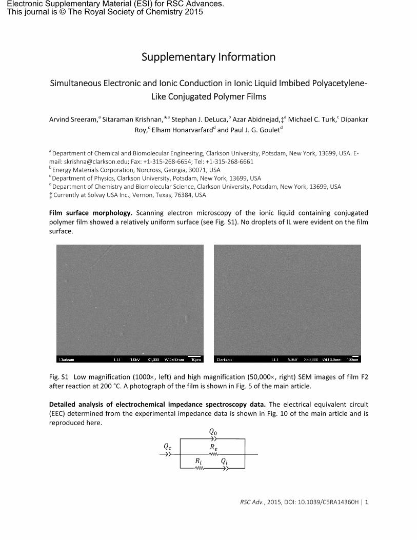
 Film  surface  morphology.  Scanning  electron  microscopy  of  the  ionic  liquid  containing  conjugated polymer film showed a relatively uniform surface (see Fig. S1). No droplets of IL were evident on the film surface.  

 

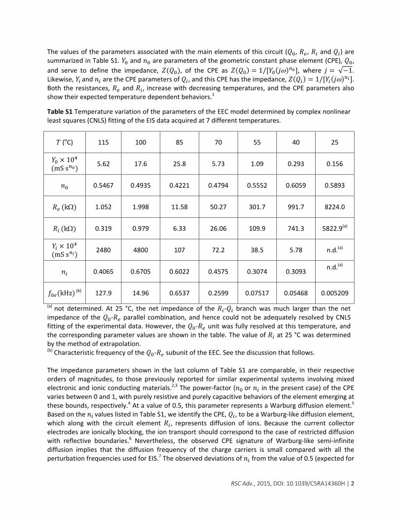
Fig. S1  Low magnification  (1000,  left) and high magnification  (50,000, right) SEM  images of  film F2 after reaction at 200 °C. A photograph of the film is shown in Fig. 5 of the main article.  Detailed  analysis  of  electrochemical  impedance  spectroscopy  data.  The  electrical  equivalent  circuit (EEC) determined from the experimental  impedance data  is shown  in Fig. 10 of the main article and  is reproduced here. 

 

Electronic Supplementary Material (ESI) for RSC Advances.This journal is © The Royal Society of Chemistry 2015

RSC Adv., 2015, DOI: 10.1039/C5RA14360H | 2 

The values of the parameters associated with the main elements of this circuit ( ,  ,   and  ) are summarized in Table S1.   and   are parameters of the geometric constant phase element (CPE),  , 

and  serve  to  define  the  impedance,  ,  of  the  CPE  as  1/ , where  √ 1. Likewise,   and   are the CPE parameters of  , and this CPE has the impedance,  1/ . Both the resistances,   and  ,  increase with decreasing temperatures, and the CPE parameters also show their expected temperature dependent behaviors.1 

Table S1 Temperature variation of the parameters of the EEC model determined by complex nonlinear least squares (CNLS) fitting of the EIS data acquired at 7 different temperatures. 

 (oC)  115  100  85  70  55  40  25 

10  mSs  

5.62  17.6  25.8  5.73  1.09  0.293  0.156 

  0.5467  0.4935  0.4221  0.4794  0.5552  0.6059  0.5893 

  k   1.052  1.998  11.58  50.27  301.7  991.7  8224.0 

  k   0.319  0.979  6.33  26.06  109.9  741.3  5822.9(a) 

10  

mSs  2480  4800  107  72.2  38.5   5.78  n.d.(a) 

  0.4065  0.6705  0.6022  0.4575  0.3074  0.3093 n.d.(a) 

 

kHz  (b)  127.9  14.96  0.6537  0.2599  0.07517  0.05468  0.005209 

(a) not determined. At 25  °C,  the net  impedance of  the  ‐  branch was much  larger  than  the net impedance of  the  ‐  parallel combination, and hence could not be adequately  resolved by CNLS fitting of the experimental data. However, the  ‐  unit was fully resolved at this temperature, and the corresponding parameter values are shown  in the table. The value of   at 25 °C was determined by the method of extrapolation. (b) Characteristic frequency of the  ‐  subunit of the EEC. See the discussion that follows.  The  impedance parameters  shown  in  the  last  column of Table S1 are comparable,  in  their  respective orders of magnitudes,  to  those previously  reported  for  similar experimental  systems  involving mixed electronic and  ionic conducting materials.2,3 The power‐factor (  or    in the present case) of the CPE varies between 0 and 1, with purely resistive and purely capacitive behaviors of the element emerging at these bounds, respectively.4 At a value of 0.5, this parameter represents a Warburg diffusion element.5 Based on the   values listed in Table S1, we identify the CPE,  , to be a Warburg‐like diffusion element, which  along with  the  circuit  element  ,  represents  diffusion  of  ions.  Because  the  current  collector electrodes are ionically blocking, the ion transport should correspond to the case of restricted diffusion with  reflective  boundaries.6  Nevertheless,  the  observed  CPE  signature  of Warburg‐like  semi‐infinite diffusion  implies  that  the  diffusion  frequency  of  the  charge  carriers  is  small  compared with  all  the perturbation frequencies used for EIS.7 The observed deviations of   from the value of 0.5 (expected for 

RSC Adv., 2015, DOI: 10.1039/C5RA14360H | 3 

an  ideal  Warburg  element)  is  attributed  to  inhomogeneous  distribution  of  diffusion  sites  in  the sample.6,8 

Unlike  the  case  of  ions,  electron  transport  in  our  measurements  is  associated  with  non‐blocking boundaries, and therefore, the parameters of the (“electron  leaking”) geometric CPE,  , are affected by  the diffusive movements of electrons. The expected Warburg‐like nature of    is validated by  the values of  , observed in the neighborhood of 0.5, as expected for a Warburg element. It is likely that, this    is a parallel  combination of  the actual geometric CPE with a Warburg‐like CPE  resulting  from electron diffusion. The latter is expected to dominate the resulting value of such a combination, because 

the intrinsic   for these systems tends to be rather small (typically in the range between 1011 and 109 S sn),2,3  which  makes  the  innate  impedance  of  the  geometric  CPE  very  large.  The  effect  of  electron diffusion on  the value of    is also suggested by  the observed  increase  in  the value of  this parameter with temperature, consistent with an expected  increase  in the diffusion coefficient with an  increase  in temperature. 

As  seen  in  Fig.  9  of  the main  article,  the  Nyquist  spectra  recorded  at  the moderate  temperatures displayed two visually separable impedance arcs formed by the   and the   subunits of the EEC.  The  specific  circuit‐blocks  linked  to  these  individual  arcs  can  be  identified  from  a  careful examination  of  the  characteristic  frequencies  (or  time  constants)  of  the  arcs.  For  a  simple  parallel combination of a  resistor and a CPE,  the characteristic  frequency would appear at  the  top  (maximum 

′′) of  the depressed semicircle generated by  the combined elements.9 However, with  the mutually overlapping  arcs  observed  in  the  present work,  it was  difficult  to  clearly  locate  these  characteristic frequencies by simple inspection. 

Therefore, in order to identify the electronic and ionic components of the recorded Nyquist plot at each temperature  setting, we  evaluated  the  characteristic  frequency of  the   block using  the CNLS‐fitted parameters. Subsequently, we traced the observed frequency spectrum to  locate the position of the  corresponding  data  point  (labeled  by  its  frequency  coordinate)  on  the  given  plot.  The   subunit of the EEC was specifically chosen for this analysis, because the  impedance parameters of this block were fully resolved in the CNLS fits at all temperatures of measurement (Table S1). In addition, this combination of elements would  lead  to a well‐defined, and hence  readily  identifiable, semicircle with whose center is located at an angle of  1 /2  below the  ′ axis. Once the Nyquist feature for this impedance contribution of electronic conduction was identified, the remaining Nyquist feature could be readily linked to ionic conduction. 

The time constant ( ) and the corresponding characteristic frequency ( ) of the   combination were calculated using:9 

⁄ 2  

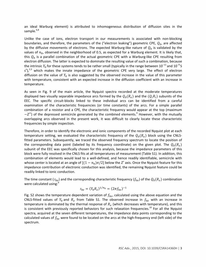
Fig. S2 shows the temperature dependent variation of  , calculated using the above equation and the CNLS‐fitted  values  of  and    from  Table  S1.  The  observed  increase  in    with  an  increase  in temperature is dominated by the thermal response of   (which decreases with temperature), and this is  consistent with previously  reported behaviors  for  such  relaxation  frequencies.10 For all  the Nyquist spectra, acquired at the seven different temperatures, the impedance data points corresponding to the calculated values of   were found to be located on the arcs at the high‐frequency end (left side) of the spectrum. 

RSC Adv., 2015, DOI: 10.1039/C5RA14360H | 4 

 

Fig. S2  Temperature dependence of the characteristic frequency,  , of the  ‐   impedance unit  in the EEC. The symbols represent data points obtained by CNLS fitting the experimental impedance data, and  the  solid  trace  is  the best‐fit  curve  for  the   vs.  temperature data. The equation used and  the overall quality of the fit (  value) are indicated in the figure. 

On  the basis of  this analysis,  it was concluded  that  the arc associated with  the higher  frequency data (left  side  of  the  Nyquist  spectrum)  in  Fig.  9  was  linked  to  electronic  conduction,  while  the  arc corresponding to the  lower frequency data (on the right side of the Nyquist plot) was associated with ionic conduction. 

Shape  of  the Nyquist  spectra  acquired  at  115  °C.  The  radius  of  the  arc  attributed  to  the  electronic conduction is proportional to  .9 From the values of   given in Table S1, it is evident that the radius of this arc would decrease with an increase in temperature. Simultaneously, because of an increase in   with temperature  (cf. Fig. S2), the top of the arc would shift toward the  left of the Nyquist spectrum, carrying with it the entire arc. At 115 °C, the top of the electronic arc was located at impedance values corresponding  to  128  kHz,  and  therefore,  at  the  very  left  end  of  the  ′  axis.  (Note  that  the  last experimental data point observed at the left‐most end of the  ′ axis in each panel of Fig. 9 was from a measurement using a perturbation frequency of 300 kHz). As a result, only a small portion of the   arc was revealed  in our measurements  (see the high‐frequency corner of the Nyquist spectrum  in Fig. 9D), while  the  remaining plot area was covered by  the arc  resulting  from  ionic conduction. Note also that the overall dimension of the ionic arc was significantly smaller for the spectrum acquired at 115 °C, compared with  the  ionic arcs observed  in  the  lower  temperature spectra. However, on  the optimized impedance scale used in Fig. 9D, the Nyquist feature of the ionic rail appears to dominate the observed spectrum. In conclusion, the impedance spectrum collected at 115 °C was predominantly the signature of the of the  ionic rail, whereas the spectrum acquired at 25 °C was, for most part, a manifestation of the  electronic  rail.  The  spectra  acquired  at  intermediate  temperatures displayed  impedance  features from both, the electronic and the ionic transport pathways. 

References 1. J. R. Macdonald, Solid State Ionics, 1984, 13, 147–149. 2. M. Wasiucionek, J. Garbarczyk, B. Wnȩtrzewski, P. Machowski and W. Jakubowski, Solid State Ionics, 1996, 92, 155–

160. 3. E. S. Matveeva, R. D. Calleja and V. Parkhutik, J. Non‐Cryst. Solids, 1998, 235, 772–780. 4. J. Jorcin, M. E. Orazem, N. Pébère and B. Tribollet, Electrochim. Acta, 2006, 51, 1473–1479. 5. E. Cuervo‐Reyes, C. P. Scheller, M. Held and U. Sennhauser, J. Electrochem. Soc., 2015, 162, A1585–A1591. 6. J. Bisquert, J. Phys. Chem. B, 2002, 106, 325–333. 7. J. Garland, D. Crain and D. Roy, Electrochim. Acta, 2014, 148, 62–72. 

20 40 60 80 100 12010

‐3

10‐2

10‐1

100

101

102

103

Temperature (oC)

f 0e (

kHz)

y = 3.37×10– 4 e0.1041x

r2 = 0.9463

RSC Adv., 2015, DOI: 10.1039/C5RA14360H | 5 

8. J. Bisquert and A. Compte, J. Electroanal. Chem., 2001, 499, 112–120. 9. G. J. Brug, A. L. G. Van Den Eeden, M. Sluyters‐Rehbach and J. H. Sluyters, J. Electroanal. Chem., 1984, 176, 275–295. 10. J. R. MacDonald, Solid State Ionics, 1985, 15, 159–161.