
Electronic and Structural Dynamics of Complex...
175
Electronic and Structural Dynamics of Complex Materials Nicky Dean Jesus College, Oxford Submitted for the degree of Doctor of Philosophy Trinity Term 2010
Transcript of Electronic and Structural Dynamics of Complex...

Electronic and Structural Dynamics ofComplex Materials
Nicky Dean
Jesus College, Oxford
Submitted for the degree of Doctor of Philosophy
Trinity Term 2010


for my family


Wake, butterfly -
It’s late,
We’ve miles to go together.
— Basho


Abstract
The time-resolved determination of dynamics in complex materials is an important goal for
understanding and controlling material properties, especially on ultrafast timescales. This
thesis reports on the development of broadband spectroscopic techniques for characterising
electronic and structural dynamics in such materials and their application to the quasi-two-
dimensional charge-density-wave Mott insulator 1T -TaS2. The experiments take two main
approaches. First, optical pump-probe spectroscopy from the terahertz to the visible regions
of the electromagnetic spectrum is used to investigate the collective response. Secondly,
time- and angle-resolved photoemission spectroscopy monitors single-electron dynamics on
the earliest timescales across the Brillouin zone.
In the photoinduced phase of TaS2, terahertz spectroscopy demonstrates an increase in
conductivity as the phase transition occurs and reveals the evolution of three phonon modes,
which undergo transient Fano reshaping due to electron-lattice interactions. Pump-probe
measurements at higher energy highlight coherent excitation of the charge density wave am-
plitude mode and the emergence of a broad resonance feature associated with polaron for-
mation in the new phase. The photoemission experiments show that photoexcitation causes
prompt collapse of the Mott gap and leads to partial unfolding of the Brillouin zone on longer
timescales, as structural distortions relax.
The emerging picture of this transient phase is one in which the Mott gap is melted but
the low-temperature symmetry is retained. Meanwhile, transport is dominated by polaronic
conductivity. This unique phase is only accessible by photo-doping.
Finally, a new method of ultrafast control, in which light is coupled to vibrational modes
of the system rather than electronic excitations, is introduced and demonstrated in the man-
ganites. An exploration of this technique using FELs promises to reveal the role of different
types of distortion in driving ultrafast processes, while phase stabilisation of excitation pulses
opens up new paths to coherent control.
vii


Role of the author
Many of the experimental results presented in this thesis were obtained in the Oxford labo-
ratory of the Cavalleri Group. Others were taken elsewhere as part of multi-national collabo-
rations. Unless otherwise clearly stated, the data acquisition and analysis was performed by
the author.
The pulse characterisation schemes in chapter 3 were built by the author, who also took
the measurements.
In chapter 4, the terahertz spectroscopy system presented was designed and built by
the author and R. Tobey. The derivation of optical constants from time-resolved terahertz
measurements was performed by the author with assistance from J. Petersen.
All of the experimental apparatus described in chapter 5 was designed and built by the
author and R. Tobey, with additional help from D. Fausti. The results presented were all
taken and analysed by the author, with helpful input from J. Petersen and S. Kaiser. L.
Gasparov provided the static FTIR data.
The time- and angle-resolved photoemission spectroscopy measurements in chapter 6 were
carried out on the Artemis beamline at the Central Laser Facility, as part of a collaboration
involving J. Petersen, S. Kaiser, the author, A. Simoncig, A. L. Cavalieri, and C. Cacho.
In chapter 7, the laboratory-based results in Pr0.7Ca0.3MnO3 were taken by R. Tobey and
the author, in collaboration with M. Rini at the Lawrence Berkeley National Laboratory, USA
and A. Cavalleri. The free electron laser experiments were carried out at the FELBE facility
at the Forschungszentrum Dresden-Rossendorf, Germany. The optical switch was designed
and built by S. Winnerl and W. Seidel. The remainder of the experimental apparatus was
designed and built by M. Gensch and the author. The data presented were acquired by M.
Gensch, the author, and N. Stojanovic, with assistance from S. Winnerl and W. Seidel. The
carrier–envelope phase stable measurements were conceived by A. Cavalleri. The apparatus
was designed and built by the author, who also took the measurements presented.
ix


Acknowledgements
To say that I have enjoyed my time as a D.Phil student is something of an understatement.
It has been an eye-opening experience which has enabled me to travel to many exciting places
all over the world. And to Long Island. For this I am deeply indebted to my supervisor,
Andrea Cavalleri, without whom I would never have stumbled upon this fascinating field of
physics. His enthusiasm seems to know no bounds, and his personal support was a great help
whenever anything was refusing to do as it was supposed to.
As far as the rest of the research group is concerned, I couldn’t have been luckier with
the selection of colleagues. Scientifically, they were invaluable, even as I stared blankly back
at them in ignorance. Special mention must go to Ron Tobey for teaching me how to put
an experiment together in the first place. Socially, they have been some of the best friends
I have ever made. The early days with Ron and Simon Wall will be fondly remembered, as
will late nights in the Hi-Lo with Julia Stahler, Jesse Petersen, Daniele Fausti, and Andreas
Dienst. I should also like to thank Jesse for still talking to me after all those endless weeks
at RAL in the cold.
As one of the loudest and most disruptive people in the Simon Room, I also owe a debt of
thanks to the rest of my office, who made it a fun and pleasant working environment. Kevin
O’Keeffe was a man of constant surprises, and I have missed Charlotte Woolley’s presence on
Saturdays dearly these last few months.
I am grateful for the support of my housemates George Duncan-Jones, Fil Wyszynski, and
Melissa Coll-Smith, who seemed to enjoy my grumbling more than anyone really ought to.
The endless gossiping and nights rounded off at the Fir Tree will be sorely missed, along with
my strolls in the park and visits to the ducks with George. I owe a great deal to Matt Gray,
who was always ready with a wrap and a bowl of soup when needed. The constitutionals, the
trips to Blackwell’s, and the hunts for pretzels came to define a large part of my life in the
last four years. I would also very much like to thank Jojo, Shani, and all the girls who broke
my heart at the Woodstock Road Deli, for keeping me in fresh supply of butter beans, pasta,
coleslaw, cheese, and basil pesto.
Finally, I would like to thank my parents and my brothers for their continued support
and encouragement through all this. I couldn’t have done it without them.
xi


Contents
1 Introduction 1
1.1 Capturing Dynamics . . . . . . . . . . . . . . . . . . . . . . . . . . . . . . . . 1
1.2 The Ultrafast Regime . . . . . . . . . . . . . . . . . . . . . . . . . . . . . . . 3
1.3 Strongly Correlated Electron Materials . . . . . . . . . . . . . . . . . . . . . . 4
1.4 Photoinduced Phenomena . . . . . . . . . . . . . . . . . . . . . . . . . . . . . 5
1.5 Characterising Ultrafast Behaviour . . . . . . . . . . . . . . . . . . . . . . . . 6
2 Tantalum Disulphide 9
2.1 Transition Metal Dichalcogenides . . . . . . . . . . . . . . . . . . . . . . . . . 9
2.2 Charge Density Waves . . . . . . . . . . . . . . . . . . . . . . . . . . . . . . . 9
2.3 Mott Insulators . . . . . . . . . . . . . . . . . . . . . . . . . . . . . . . . . . . 12
2.4 Tantalum Disulphide . . . . . . . . . . . . . . . . . . . . . . . . . . . . . . . . 13
2.4.1 Basic properties . . . . . . . . . . . . . . . . . . . . . . . . . . . . . . 13
2.4.2 Thermal phases of 1T -TaS2 . . . . . . . . . . . . . . . . . . . . . . . . 15
2.4.3 Effects of commensuration . . . . . . . . . . . . . . . . . . . . . . . . . 16
2.4.4 Time-resolved studies . . . . . . . . . . . . . . . . . . . . . . . . . . . 18
3 Aspects of Ultrafast Spectroscopy 21
3.1 Ultrafast Sources . . . . . . . . . . . . . . . . . . . . . . . . . . . . . . . . . . 21
3.2 Optical Parametric Amplifiers . . . . . . . . . . . . . . . . . . . . . . . . . . . 22
3.2.1 Nonlinear optics . . . . . . . . . . . . . . . . . . . . . . . . . . . . . . 22
3.2.2 Optical parametric amplification . . . . . . . . . . . . . . . . . . . . . 23
3.2.3 Design of the infrared optical parametric amplifier . . . . . . . . . . . 24
3.2.4 Determining the wavelength . . . . . . . . . . . . . . . . . . . . . . . . 26
3.2.5 Determining the pulse duration . . . . . . . . . . . . . . . . . . . . . . 28
3.3 Pump-Probe Spectroscopy . . . . . . . . . . . . . . . . . . . . . . . . . . . . . 30
3.4 Anatomy of Transient Reflectivity Measurements . . . . . . . . . . . . . . . . 32
3.4.1 Timescales . . . . . . . . . . . . . . . . . . . . . . . . . . . . . . . . . 32
xiii

xiv Contents
3.4.2 Coherent phonons . . . . . . . . . . . . . . . . . . . . . . . . . . . . . 32
3.5 Summary . . . . . . . . . . . . . . . . . . . . . . . . . . . . . . . . . . . . . . 34
4 Terahertz Time-Domain Spectroscopy 35
4.1 The Terahertz Domain . . . . . . . . . . . . . . . . . . . . . . . . . . . . . . . 35
4.2 Generation and Detection . . . . . . . . . . . . . . . . . . . . . . . . . . . . . 36
4.3 Determining the Optical Properties . . . . . . . . . . . . . . . . . . . . . . . . 40
4.3.1 The complex optical constants . . . . . . . . . . . . . . . . . . . . . . 40
4.3.2 Fresnel’s relations . . . . . . . . . . . . . . . . . . . . . . . . . . . . . 41
4.3.3 Analysis of THz-TDS measurements . . . . . . . . . . . . . . . . . . . 42
4.3.4 The phase problem . . . . . . . . . . . . . . . . . . . . . . . . . . . . . 44
4.4 Time-Resolved Terahertz Time-Domain Spectroscopy . . . . . . . . . . . . . . 45
4.4.1 Acquisition complications . . . . . . . . . . . . . . . . . . . . . . . . . 45
4.5 Determining the Transient Optical Properties . . . . . . . . . . . . . . . . . . 48
4.6 Summary . . . . . . . . . . . . . . . . . . . . . . . . . . . . . . . . . . . . . . 51
5 The Photoinduced Phase of 1T -TaS2 53
5.1 Ultrafast Dynamics in 1T -TaS2 . . . . . . . . . . . . . . . . . . . . . . . . . . 53
5.2 Fano Resonances . . . . . . . . . . . . . . . . . . . . . . . . . . . . . . . . . . 54
5.3 Terahertz Experiments . . . . . . . . . . . . . . . . . . . . . . . . . . . . . . . 58
5.3.1 Experimental setup . . . . . . . . . . . . . . . . . . . . . . . . . . . . . 58
5.3.2 Static measurements . . . . . . . . . . . . . . . . . . . . . . . . . . . . 60
5.3.3 Time-resolved measurements . . . . . . . . . . . . . . . . . . . . . . . 65
5.4 Infrared Experiments . . . . . . . . . . . . . . . . . . . . . . . . . . . . . . . . 72
5.4.1 Experimental setup . . . . . . . . . . . . . . . . . . . . . . . . . . . . . 72
5.4.2 Near-infrared response . . . . . . . . . . . . . . . . . . . . . . . . . . . 75
5.4.3 Broadband infrared response . . . . . . . . . . . . . . . . . . . . . . . 81
5.5 Evidence for Polaronic Conductivity . . . . . . . . . . . . . . . . . . . . . . . 84
5.5.1 Polarons . . . . . . . . . . . . . . . . . . . . . . . . . . . . . . . . . . . 84
5.5.2 Polaronic conductivity in the photoinduced phase of TaS2 . . . . . . . 86
5.6 Summary . . . . . . . . . . . . . . . . . . . . . . . . . . . . . . . . . . . . . . 89
6 Time- and Angle-Resolved Photoemission Spectroscopy of 1T -TaS2 91
6.1 Angle-Resolved Photoemission Spectroscopy . . . . . . . . . . . . . . . . . . . 91
6.2 Time- and Angle-Resolved Photoemission Spectroscopy . . . . . . . . . . . . 94
6.3 Photoemission spectroscopy of TaS2 . . . . . . . . . . . . . . . . . . . . . . . 95
6.4 TARPES Experiments in TaS2 . . . . . . . . . . . . . . . . . . . . . . . . . . 96
6.4.1 Experimental setup . . . . . . . . . . . . . . . . . . . . . . . . . . . . . 96

Contents xv
6.4.2 Static measurements . . . . . . . . . . . . . . . . . . . . . . . . . . . . 99
6.4.3 Time-resolved measurements . . . . . . . . . . . . . . . . . . . . . . . 101
6.5 Summary . . . . . . . . . . . . . . . . . . . . . . . . . . . . . . . . . . . . . . 107
7 Vibrational Excitation of Complex Materials 109
7.1 A New Approach . . . . . . . . . . . . . . . . . . . . . . . . . . . . . . . . . . 109
7.2 Manganites . . . . . . . . . . . . . . . . . . . . . . . . . . . . . . . . . . . . . 110
7.2.1 Basic properties . . . . . . . . . . . . . . . . . . . . . . . . . . . . . . 110
7.2.2 Phase transitions . . . . . . . . . . . . . . . . . . . . . . . . . . . . . . 112
7.3 Pr1−xCaxMnO3 . . . . . . . . . . . . . . . . . . . . . . . . . . . . . . . . . . . 114
7.4 Vibrational Control Experiments . . . . . . . . . . . . . . . . . . . . . . . . . 115
7.4.1 Experimental setup . . . . . . . . . . . . . . . . . . . . . . . . . . . . . 115
7.4.2 Experimental results . . . . . . . . . . . . . . . . . . . . . . . . . . . . 117
7.4.3 The next steps . . . . . . . . . . . . . . . . . . . . . . . . . . . . . . . 120
7.5 Studying Resonant Effects . . . . . . . . . . . . . . . . . . . . . . . . . . . . . 120
7.5.1 Laboratory limitations . . . . . . . . . . . . . . . . . . . . . . . . . . . 120
7.5.2 Free electron lasers . . . . . . . . . . . . . . . . . . . . . . . . . . . . . 121
7.5.3 Experiments at FELBE . . . . . . . . . . . . . . . . . . . . . . . . . . 122
7.5.4 Experimental results . . . . . . . . . . . . . . . . . . . . . . . . . . . . 124
7.5.5 Further measurements . . . . . . . . . . . . . . . . . . . . . . . . . . . 126
7.6 Field-Resolved Effects . . . . . . . . . . . . . . . . . . . . . . . . . . . . . . . 128
7.7 Summary . . . . . . . . . . . . . . . . . . . . . . . . . . . . . . . . . . . . . . 131
8 Conclusion and Future Directions 133
8.1 Overview . . . . . . . . . . . . . . . . . . . . . . . . . . . . . . . . . . . . . . 133
8.1.1 Tantalum disulphide . . . . . . . . . . . . . . . . . . . . . . . . . . . . 133
8.1.2 Vibrational excitation . . . . . . . . . . . . . . . . . . . . . . . . . . . 135
8.2 Looking Ahead . . . . . . . . . . . . . . . . . . . . . . . . . . . . . . . . . . . 135
8.2.1 Tantalum disulphide . . . . . . . . . . . . . . . . . . . . . . . . . . . . 135
8.2.2 Vibrational excitation . . . . . . . . . . . . . . . . . . . . . . . . . . . 136
8.2.3 Further afield . . . . . . . . . . . . . . . . . . . . . . . . . . . . . . . . 137
8.3 Final Remarks . . . . . . . . . . . . . . . . . . . . . . . . . . . . . . . . . . . 138
Bibliography 139


Figures
1 Introduction 1
1.1 ‘Plate Number 156. Jumping; running straight high jump’ by Eadweard Muy-
bridge . . . . . . . . . . . . . . . . . . . . . . . . . . . . . . . . . . . . . . . . 2
2 Tantalum Disulphide 9
2.1 The Peierls distortion in a 1D metal . . . . . . . . . . . . . . . . . . . . . . . 10
2.2 Excitations of the charge density wave state . . . . . . . . . . . . . . . . . . . 11
2.3 Structure of 1T -TaS2 . . . . . . . . . . . . . . . . . . . . . . . . . . . . . . . . 14
2.4 Resistivity of TaS2 as a function of temperature . . . . . . . . . . . . . . . . . 15
2.5 Schematic representation of the band structure of 1T -TaS2 . . . . . . . . . . 16
2.6 Optical conductivity of TaS2 for a variety of temperatures in the QC and C
phases . . . . . . . . . . . . . . . . . . . . . . . . . . . . . . . . . . . . . . . . 17
3 Aspects of Ultrafast Spectroscopy 21
3.1 Schematic diagram of a near-infrared optical parametric amplifier . . . . . . . 24
3.2 Measuring wavelengths . . . . . . . . . . . . . . . . . . . . . . . . . . . . . . . 27
3.3 Determining pulse durations . . . . . . . . . . . . . . . . . . . . . . . . . . . . 29
4 Terahertz Time-Domain Spectroscopy 35
4.1 Schematic layout for free-space electro-optic sampling . . . . . . . . . . . . . 37
4.2 Schematic layout for a THz time-domain spectrometer . . . . . . . . . . . . . 38
4.3 THz time-domain traces and associated spectra . . . . . . . . . . . . . . . . . 39
4.4 Reflection and refraction of electromagnetic waves at the interface between
two media . . . . . . . . . . . . . . . . . . . . . . . . . . . . . . . . . . . . . . 41
4.5 Schematic setup for a time-resolved THz time-domain spectrometer operating
in transmission . . . . . . . . . . . . . . . . . . . . . . . . . . . . . . . . . . . 46
4.6 Effect of delay lines in TRTS . . . . . . . . . . . . . . . . . . . . . . . . . . . 47
xvii

xviii Figures
4.7 Approximating a photoexcited sample by a thin film on an unexcited sample
substrate . . . . . . . . . . . . . . . . . . . . . . . . . . . . . . . . . . . . . . 49
5 The Photoinduced Phase of 1T -TaS2 53
5.1 Fano lineshapes for different asymmetry parameters q . . . . . . . . . . . . . 56
5.2 Fano conductivity profiles . . . . . . . . . . . . . . . . . . . . . . . . . . . . . 58
5.3 Experimental layout for the time-resolved THz spectroscopy measurements . 60
5.4 Temperature-resolved THz measurements on TaS2 . . . . . . . . . . . . . . . 61
5.5 Complex conductivity σ(ω) of TaS2 obtained at 15K . . . . . . . . . . . . . . 63
5.6 THz traces acquired from TaS2 . . . . . . . . . . . . . . . . . . . . . . . . . . 66
5.7 Photoinduced conductivity σ1(ω) . . . . . . . . . . . . . . . . . . . . . . . . . 68
5.8 Temporal and intensity dependent behaviour of σ1(ω) . . . . . . . . . . . . . 69
5.9 Temporal evolution of the 1.6THz mode . . . . . . . . . . . . . . . . . . . . . 70
5.10 Time-dependent asymmetry parameter and renormalised mode frequency . . 71
5.11 Experimental layout for the infrared pump-probe measurements . . . . . . . . 73
5.12 Pump-induced changes in reflectance for TaS2 at 15K . . . . . . . . . . . . . 75
5.13 Fourier transforms of the coherent oscillations in ∆R(t)/R . . . . . . . . . . . 76
5.14 Fit to the data at 0.62 eV after excitation with 1.4mJ cm−2 pump intensity . 77
5.15 Intensity dependence of the fit coefficients at 0.62 eV probe energy . . . . . . 79
5.16 Pump-probe traces for different probe photon energies . . . . . . . . . . . . . 81
5.17 Intensity dependence of the fit coefficients at all probe energies . . . . . . . . 82
5.18 Peak reflectance changes at 0 ps as a function of probe energy . . . . . . . . . 83
5.19 Diagrammatic representation of a polaron . . . . . . . . . . . . . . . . . . . . 85
5.20 Comparison of the phases of TaS2 . . . . . . . . . . . . . . . . . . . . . . . . 87
6 Time- and Angle-Resolved Photoemission Spectroscopy of 1T -TaS2 91
6.1 The relationship between the energy levels in a solid and the photoemission
spectrum . . . . . . . . . . . . . . . . . . . . . . . . . . . . . . . . . . . . . . 92
6.2 Schematic representation of an ARPES experiment . . . . . . . . . . . . . . . 93
6.3 Schematic of the TARPES beamline layout . . . . . . . . . . . . . . . . . . . 97
6.4 Real and reciprocal space structures of TaS2 . . . . . . . . . . . . . . . . . . . 99
6.5 Static photoemission intensity maps and energy distribution curves for the
low-temperature phase of TaS2 . . . . . . . . . . . . . . . . . . . . . . . . . . 100
6.6 Temporal behaviour of the electronic structure . . . . . . . . . . . . . . . . . 102
6.7 Evolution of the bands through the photoinduced phase transition . . . . . . 103
6.8 Variation of dynamics over the full range of energies at the Γ and M points . 105
6.9 Spectral distribution of changes to band structure on electronic and structural
timescales . . . . . . . . . . . . . . . . . . . . . . . . . . . . . . . . . . . . . . 106

Figures xix
7 Vibrational Excitation of Complex Materials 109
7.1 The ideal unit cell of an ABO3 perovskite . . . . . . . . . . . . . . . . . . . . 110
7.2 Schematic representation of the d-level electronic structure in the presence of
a crystal field . . . . . . . . . . . . . . . . . . . . . . . . . . . . . . . . . . . . 111
7.3 Properties of manganites . . . . . . . . . . . . . . . . . . . . . . . . . . . . . . 113
7.4 The properties of Pr1−xCaxMnO3 . . . . . . . . . . . . . . . . . . . . . . . . . 114
7.5 Optical conductivity spectrum of Pr0.7Ca0.3MnO3 . . . . . . . . . . . . . . . 116
7.6 Schematic layout for the vibrational control experiment in PCMO . . . . . . 117
7.7 Reflectance changes for PCMO after photoexcitation with mid-IR radiation . 118
7.8 Schematic layout of the FEL at FELBE . . . . . . . . . . . . . . . . . . . . . 122
7.9 Using the optical switch to change the FEL repetition rate . . . . . . . . . . . 123
7.10 Schematic layout for the FELBE experiments . . . . . . . . . . . . . . . . . . 125
7.11 Reflectance changes for PCMO after photoexcitation with FEL radiation . . 127
7.12 Illustration of the carrier-envelope phase evolution from pulse to pulse . . . . 129
7.13 A carrier-envelope phase stable pulse generated by DFG between two OPAs . 130


Chapter 1
Introduction
1.1 Capturing Dynamics
This year sees the fiftieth anniversary of the laser, and while it may have started out life
as a scientific curiosity, the great ‘solution looking for a problem’ [1], it has since become
one of the most ubiquitous pieces of technology in existence, finding a home for itself in
environments as diverse as the research laboratory, the hospital, and the living room. At
its birth, many considered the laser as little more than a death ray [2], undoubtedly fuelled
by Cold War paranoia [3]. Scientists working on laser development had other ideas. Shortly
after demonstrating the first working laser [4], Theodore Maiman described the five potential
applications he foresaw for his creation: (i) true amplification of light; (ii) increasing the
number of communication channels; (iii) probing matter for basic research; (iv) high-power
beams for space communications; (v) concentrating light for industry, chemistry, and medicine
[5].
With the subsequent decades of intense laser research and development, the probing of
matter has become an important area of research for the laser. This is especially true with
pulsed lasers, which can be used to trigger and measure dynamical behaviour in solids on
extremely fast timescales.
Such time-resolved measurements capture snapshots of an event as it happens, which can
then be built up into a full sequence, mapping out exactly what is going on at any given time.
In the late 19th century, Eadweard Muybridge performed one of the first ever time-resolved
1

2 1.1. Capturing Dynamics
Figure 1.1: ‘Plate Number 156. Jumping; running straight high jump’ by Eadweard Muy-
bridge (1887), courtesy of Corcoran Gallery of Art, Washington, DC [6]. These early time-
resolved photographs were used to understand dynamical motion of people and animals.
experiments when he captured Leland Stanford’s horse in motion, settling the debate as to
whether or not a horse’s hooves are ever all off the ground at the same time. Muybridge used
a series of cameras with high shutter speeds, each triggered by a trip wire, to capture the
horse at different points in its gallop. Each exposure was short enough to clearly capture the
horse at a distinct point in its motion, revealing for the first time the nature of its movements,
previously too fast to be resolved by the eye. Muybridge went on to capture an enormous
number of dynamical events from both animals and humans, unveiling their actions for all to
see [7]; an example of such a measurement is shown in figure 1.1.
This concept can be applied to laser-based time-resolved experiments used to study physi-
cal, chemical, and biological processes. In the contemporary version of Muybridge’s measure-
ments, the cameras are replaced by laser pulse trains, with their short pulse durations acting
as the high-speed ‘shutters’. A first intense pulse is used to initiate dynamics in the system
under scrutiny. Then a second laser pulse interacts with the system, becoming encoded with
information about its properties at the moment of arrival. By changing the relative time
delay between the pulses a series of snapshots is created, providing an image of the system’s
evolution, much like Muybridge’s images captured their subjects in motion. This technique
lies at the heart of the pump-probe experiment.

Chapter 1. Introduction 3
In order for these snapshots to be of any use, regardless of the century, they need to
clearly resolve what they are measuring. Any image taken of a dynamic event captures its
progress throughout the exposure time. If the system being observed is changing during this
period, then the image gets blurred, and whilst this leads to interesting photographic effects,
it is not helpful in providing information on what is actually happening. Thus it becomes
crucial to reduce the exposure time to a timescale comparable to or shorter than the event
taking place. It is this principal which allowed Muybridge to understand the movements of
racehorses and which allows scientists to understand the motion of atoms and electrons in all
manner of processes around us.
1.2 The Ultrafast Regime
Time-resolved science has garnered two Nobel Prizes, marking important milestones in the
speed with which dynamical events can be recorded. In 1967, the Nobel Prize in Chemistry
was awarded to Manfred Eigen, Ronald G.W. Norrish, and George Porter ‘for their studies
of extremely fast chemical reactions, effected by disturbing the equilibrium by means of very
short pulses of energy’ [8]. They were able to monitor chemical reactions taking place on
microsecond (10−6 seconds) and nanosecond (10−9 seconds) timescales. The rapid growth
in femtosecond technology in the ’80s and ’90s paved the way for the second prize, awarded
to Ahmed Zewail in 1999 ‘for his studies of the transition states of chemical reactions using
femtosecond spectroscopy’ [8]. By using light in a manner similar to that described earlier,
Zewail was able to capture reactions taking place on picosecond (ps, 10−12 seconds) and
femtosecond (fs, 10−15 seconds) timescales.
Processes occurring on such short timescales are referred to as ‘ultrafast’ processes. They
include not only chemical reactions, but also many operations taking place in solid state
systems, where the nature of interactions and ordering in a crystal gives rise to an abundance
of ultrafast effects. The continuing development of ultrafast laser sources, and the ever-
shorter probes they provide, has enabled a great deal of progress to be made in observing
and understanding these fundamental processes, extending the approach of Zewail in new and
exciting directions.
In addition to studying underlying interactions, ultrafast technology has opened up the
ability to control matter in new ways. Using laser radiation, material systems can be driven

4 1.3. Strongly Correlated Electron Materials
into new non-equilibrium states, inaccessible by more traditional methods. The properties of
these new meta-stable phases can be controlled and altered by varying the properties of the
driving laser, suggesting a wealth of potential technological applications based on short-lived
or rapidly-changing effects.
1.3 Strongly Correlated Electron Materials
Oftentimes, when trying to describe the electronic properties of solids, conventional band
theory is invoked. Within this framework, electron-electron interactions are ignored and each
electron is treated as independent from the rest. The electrons occupy atomic orbitals, which
form a set of discrete energy levels. When the atoms are brought into a crystal formation,
these energy levels become very close and form bands, which are separated by energy gaps.
The number of electrons in a band and the size of the gap separating successive bands dictates
the properties of the solid. Band theory has proved immensely successful at describing the
electronic properties of many materials, such as metals, insulators, and semiconductors.
However, this independent-electron model is only an approximation to the true behaviour,
albeit a very good one in many cases. In reality, the electrons are interacting with one
another all the time. As the strength of the interactions becomes increasingly important,
the independent-electron picture begins to break down and the predictions of band theory no
longer match the observed behaviour. This is the realm of strongly correlated electron, or
complex, materials. These are materials in which the Coulomb interaction between electrons
is larger than their kinetic energy, meaning an electron remains on a given lattice site long
enough to feel the presence of other electrons nearby. This results in a large number of exotic
ordered states and unusual phase transitions. The properties of such materials are often vastly
different to those predicted by conventional band theory [9, 10].
In general, it is not just the inter-electron correlations which are important, but also the
correlation between the electrons and many other degrees of freedom, such as the lattice.
The ground state properties of a complex material are then determined by the competition
between these various interactions. If several different couplings are competing on similar
energy scales, then these properties become very sensitive to subtle perturbations, resulting
in a variety of different phases. This complex interplay produces such fascinating effects as
superconductivity, where electron-lattice coupling not only reduces the electronic bandwidth,

Chapter 1. Introduction 5
but also creates an attractive force between the electrons, leading to the formation of Cooper
pairs [11].
The properties of correlated materials can be controlled by changing the strength of differ-
ent interactions, causing some to become more prevalent than others. Typically, this involves
the application of pressure or magnetic or electric fields, varying the temperature, or chemical
doping, which adds or removes electrons from the system. Tipping the balance in this way
produces interesting phase transitions separated by only small differences in energy [12]. Un-
derstanding the nature of these couplings is vital to understanding the macroscopic behaviour
of the material.
1.4 Photoinduced Phenomena
In addition to those methods of control mentioned above, the properties of a material can also
be perturbed using light. Unlike those methods, photoexcitation is a non-adiabatic process,
shaking the system up in a highly non-equilibrium fashion. The effects of photoexcitation
can vary depending on the material properties and nature of the light used, and range from
simple carrier excitation to photoinduced structural and electronic phase transitions. Many
different types of dynamics can arise from photoexcitation, and studying them can reveal a
lot about the nature of the underlying interactions in the solid.
Photoexcitation has been used in semiconductors for a long time to understand carrier
relaxation and early-timescale dynamics in both absorption spectroscopy [13, 14] and, more
recently, THz spectroscopy [15]. The parallels between photoexcitation and chemical doping
have led to the process often being described as ‘photo-doping’ [16].
Light is also frequently used for controlling the behaviour of a material through photoin-
duced phase transitions [17]. In these types of transition, excitation of electrons upsets the
interplay between degrees of freedom, driving the system into a new regime where its proper-
ties can become quite different: structural relaxation can take place, shifting the positions of
ions towards some new symmetry position [18–20], the optical properties can undergo large-
scale changes [21], and metallic states can be formed [22]. All of these effects last for only
fractions of a second, with the system eventually relaxing back to its equilibrium state.

6 1.5. Characterising Ultrafast Behaviour
1.5 Characterising Ultrafast Behaviour
The range of tools available for studying ultrafast processes has blossomed in the last couple
of decades. The frontiers of ultrafast science continue to explore ever shorter timescales,
studying effects on the scale of a few femtoseconds [23, 24] and pushing on into the attosecond
(10−18 seconds) regime [25]. Observing the collapse of gaps after photoexcitation on the
fastest timescales and clocking the rate at which processes occur can reveal a great deal of
information on the formation of states in complex materials.
However, whilst these endeavours provide insight into the fundamental timescales and
electronic interactions, there is still the important task of characterising the dynamics of
photoinduced phases in solids. In the same way that it is important to fully determine the
equilibrium properties of a material by studying its electrodynamic response over a broad en-
ergy range, a full understanding of photoinduced phenomena can only be attained by looking
across different energy scales. This requires an array of different ultrafast probes covering
large portions of the electromagnetic spectrum, from terahertz (THz, 1012 Hz) frequencies,
up through the infrared and visible spectrum, and into the ultraviolet and X-ray regions.
Time-resolved analogues of established static techniques such as X-ray diffraction, which
can provide information on the ordering of electronic states [26, 27], and photoelectron spec-
troscopy, which maps out the band structure as photoinduced processes occur [28, 29], are
powerful tools in approaching a fuller appreciation of the effects of photoexcitation.
It is the aim of this thesis to develop a series of sophisticated characterisation techniques to
produce a more detailed depiction of the photoinduced phases of complex materials, focussing
on the intriguing Mott-insulating charge-density-wave compound 1T -TaS2. This necessitates
the use of a variety of different ultrafast probes, all based on the same stroboscopic experi-
mental principal outlined at the start of this chapter, making use of photon energies from the
milli-electron volt scale up to tens of electron volts.
The methods employed will take two routes, each of which interrogates the system in a
slightly different manner. Broadband optical spectroscopy measurements offer insight into
the transport properties and collective behaviour of the system, capturing dynamics between
1meV and 1 eV during the first few picoseconds after photoexcitation. Meanwhile, time- and
angle-resolved photoelectron spectroscopy gives information on the single particle picture,

Chapter 1. Introduction 7
providing momentum-resolved snapshots of the evolution of the electronic band structure
during the onset of the photoinduced phase transition. The combination of these techniques
allows for detailed characterisation of the electronic and structural dynamics of photoinduced
phases in complex materials. By widening the window over which ultrafast processes are
observed, a richer understanding of the exotic phases accessible with light may be achieved.


Chapter 2
Tantalum Disulphide
2.1 Transition Metal Dichalcogenides
Throughout the 1960s and 1970s, layered transition metal dichalcogenides were the subject
of intense experimental scrutiny [30, 31], and they continue to find themselves constantly
under the microscope to this day [32–38]. This class of materials is interesting due to its
two-dimensional behaviour, which results in a wide variety of phenomena, from ordinary
insulating and metallic behaviour, to semimetallic and superconducting properties [30, 38].
It has also proven a rich hunting ground for various types of charge and spin density wave
ordering [39–41], as well as Mott and Peierls transitions [42, 43].
Two phenomena have emerged as the dominant features of transition metal dichalco-
genides: the formation of various types of charge density wave state and the existence of a
Mott insulating phase at low temperatures. This chapter will first discuss these phenomena in
more detail, before elaborating further on a specific transition metal dichalcogenide, 1T -TaS2,
in which these two effects play a key role.
2.2 Charge Density Waves
In materials with highly anisotropic band structures, electron-electron and electron-phonon
interactions can lead to new ground states and collective excitations known as charge density
waves (CDWs). Such ground states occur predominantly in low-dimensional materials, and
are especially prevalent in one-dimensional systems [43, 44]. Their name aptly describes the
9

10 2.2. Charge Density Waves
EF
kF-kF0 p/a- /ap
a
r(r) r(r)
2a
kF-kF 0 p/a- /ap
D
E(k) E(k)
k k
Figure 2.1: The Peierls distortion in a 1D metal. Left: undistorted metal chain. Right: the
Peierls distortion turns the metal into an insulator. Light blue lines at the top of the figure
show the spatial charge density, ρ(r), and orange dots represent atoms. The lower portion
describes the dispersion relation in both cases, with red lines indicating occupied states.
salient feature of the CDW ground state: a periodic charge density modulation throughout
the crystal, accompanied by a periodic lattice distortion.
The formation of the CDW is usually explained through the simple one-dimensional model
of the Peierls transition [45]. In the absence of electron-electron and electron-phonon inter-
actions, a linear chain of atoms is separated by a distance a, with each atom representing a
lattice point and with one atom per unit cell. The electrons occupy states up to the Fermi
energy EF , and the dispersion relation is that of a free electron gas. This situation is illus-
trated on the left of figure 2.1. If an electron-phonon interaction is introduced and the chain
is distorted to shift every other atom slightly, as shown in the top right of figure 2.1, then
the unit cell doubles in size, halving the Brillouin zone. A gap opens at the new Brillouin
zone boundary, k = π/2a, turning the previously metallic chain into an insulator. In this
one-dimensional case, the reduction in energy at the Fermi surface is greater than the elastic
energy required for the lattice distortion [46], meaning a one-dimensional chain cannot be a
metal.
The other consequence of the modified dispersion relation is a modulation of the charge
density along the chain. As indicated in the top right of figure 2.1, the periodic lattice
distortion creates a spatially varying distribution of charge of the form cos(ρx + ϕ). This

Chapter 2. Tantalum Disulphide 11
AmplitudeMode
PhaseMode
Figure 2.2: Excitations of the charge density wave state. Lines show changes to the charge
density whilst dots are the ions. Arrows indicate the changes in the ion position.
charge density is associated with a new collective mode of the condensate called the charge
density wave [44, 46].
The spatial modulations of electronic density and lattice displacement of the CDW state
are described by a complex order parameter Ψ ∝ ∆eiϕ, much like superconductors. This
makes it possible to have excitations of both amplitude (∆) and phase (ϕ). These two
modes can be seen in figure 2.2 for the k = 0 case. Phase excitations, or phasons, represent
translations of the condensate (in the limit of k = 0). The electronic charge density is
displaced relative to the ions, resulting in a dipole moment, so the phason is optically active.
Amplitude excitations, or amplitudons, represent changes in the charge density amplitude
throughout the lattice. There is no displacement of the charge density relative to the ions,
and so no dipole moment; as such, amplitudons are Raman active [44].
CDW materials are intensely studied, especially due to their close connection with su-
perconductivity [47, 48]. They also provide an ideal playground for time-resolved studies,
where the excitation of the CDW modes or collapse of the CDW gap leads to understanding
of the collective behaviour of the system [35, 49]. Their prominent role in the transition
metal dichalcogenides, and TaS2 in particular, make a basic understanding of their properties
essential.

12 2.3. Mott Insulators
2.3 Mott Insulators
Band theory is enormously successful at describing the electronic properties of materials where
electrons can be treated as independent from one another. However, as electron correlations
become stronger, this theory begins to break down and the measured properties can become
vastly different from the predictions. This was first noticed in the case of transition metal
oxides by de Boer and Verwey [50]. A class of these compounds have only partially filled
3d bands, and so in the context of band theory they should be conductors; in fact, they
turn out to be insulators. This was subsequently explained by considering electron-electron
interactions [51].
Mott went on to describe how electron-electron interactions could suppress metallic be-
haviour in favour of an insulating state in NiO [9]. If an electron hops from one atom to
another, it leaves behind it a positively charged hole. The electron and hole attract each other
with a force resulting from the potential U ∝ −e2/r, where e is the electron charge and r is the
electron-hole separation. Mott reasoned that the existence of electron-hole pairs would screen
the field between an electron and a hole, reducing the potential to U ∝ −(e2/r) exp(−qr),
where q depends on the density of electron-hole pairs. If the density of pairs becomes large
enough then the potential U will no longer support bound states of electrons and holes and
the system can conduct. Crucially, it is the Coulomb potential which is the dominant factor,
with a large U causing electrons to be localised on-site.
Hubbard took Mott’s ideas and used them to formulate an approximate model for the
Hamiltonian of a system with strong electron-electron interactions, demonstrating how the
transition between the localised and non-localised states may occur. The theory produced
the Mott-Hubbard Hamiltonian [52]:
H = −t∑
<i,j>,σ
(c†i,σcj,σ + h.c.) + U
N∑i=1
ni,↑ni,↓. (2.1)
The first term comes from the tight-binding approximation of band theory and describes
the kinetic energy of the electrons, where t is the transfer integral, representing the inter-site
hopping of electrons, and c†i,σ, ci,σ are the creation and annihilation operators for an electron
at site i with spin up or down (σ =↑, ↓). t depends on the atomic separation and on the
particular orbitals the electrons occupy.

Chapter 2. Tantalum Disulphide 13
The second term in the Hamiltonian arises from the on-site Coulomb repulsion of the
electrons, and hence takes into account Mott’s consideration of electron-electron interactions.
U represents the Coulomb potential of two electrons on the same lattice site and ni,σ = c†i,σci,σ
is the electron number operator for the spin state σ.
From this model, it may be seen that the competition between t and U drives the system
between two different states, as initially described by Mott. When t≫ U , such that the mu-
tual electron repulsion is weak compared to the kinetic energy, the system behaves according
to the tight-binding model and band theory adequately describes its behaviour. In the other
limit, U ≫ t, the Coulomb repulsion prevents electrons from moving to occupied sites and
the charges become localised. This leads to the formation of a Mott insulator, when band
theory predicts metallic behaviour but the electron-electron repulsion is dominant, causing a
gap to open of size
Eg = U − 2Nt, (2.2)
where N is the number of nearest-neighbour atoms.
Mott insulators are of great importance in understanding the interplay between electron-
electron and electron-lattice interactions. They are significant to the work of this thesis since
the ground state of TaS2 exhibits both charge density wave and Mott characteristics, which
respond independently to photoexcitation, leading to an exotic phase of this material which
cannot be reached in equilibrium.
2.4 Tantalum Disulphide
2.4.1 Basic properties
Transition metal dichalcogenides have the basic chemical structure MX2, where M is a tran-
sition metal and X a chalcogenide. Structurally, they form sheets of X–M–X sandwiches,
which are loosely bound together by van der Waals forces; it is this weak interlayer coupling
which provides the quasi-two-dimensional character. Within the sandwich, the coordination
of the metal atom may be octahedral or trigonal prismatic, and the different possible sand-
wich stackings result in a large number of possible polytypes, the simplest two of which are
the pure octahedral (1T ) and pure trigonal prismatic (2H) structures. However, all MX2 ma-
terials share hexagonal symmetry. It is this wide variation in structural as well as chemical

14 2.4. Tantalum Disulphide
S
Ta
(a) (b)
aa
c
a
a
Figure 2.3: Structure of 1T -TaS2. Unit cell dimensions: a = 3.36 A, c = 5.90 A [53]. (a)
Octahedral coordination unit forming the S–Ta–S sandwiches. (b) The Ta plane. Without
the CDW, the unit cell is that shown by the dashed line in the upper left corner. With the
CDW, “Star of David” cluster formation takes place, shown by the solid lines. Arrows show
the displacement of Ta atoms and the dashed line connecting the stars gives the new unit
cell.
properties which leads to the myriad opportunities for experimental study.
Of all the quasi-two-dimensional transition metal dichalcogenides, the 1T polytype of
tantalum disulphide, 1T -TaS2(hereafter referred to simply as TaS2), is one of the most widely
studied. Its basic structure is shown in figure 2.3(a). Historically, it is notable for being the
among the first two-dimensional materials in which a charge density wave was observed [31].
It also becomes Mott insulating at low temperature [54], which is intimately connected to
the CDW behaviour. A number of studies have been carried out on this material, including
low-energy electron diffraction [55], photoemission spectroscopy [34, 56, 57], Fourier transform
infrared spectroscopy [58–60], Raman spectroscopy [32, 33, 61], and pump-probe spectroscopy
[28, 35], all in the hope of understanding the relationship between the charge density wave
behaviour and the Mott physics in this peculiar compound.

Chapter 2. Tantalum Disulphide 15
0 100 200 300 400
10-3
10-2
I
QC
( c
m)
Temperature (K)
C
Figure 2.4: Resistivity of TaS2 as a function of temperature for the CDW phases, taken
from [53]. C, QC, and I denote commensurate, quasicommensurate, and incommensurate
phases, respectively. The three phases can be distinguished by the abrupt hysteretic changes
in resistivity. The arrows indicate the paths for heating and cooling.
2.4.2 Thermal phases of 1T -TaS2
TaS2 has four thermodynamic phases, separated by first-order phase transitions, and differ-
entiated by significant differences in resistivity [53] and CDW commensuration [54, 57]. At
high temperatures, T > 550K, TaS2 is metallic and no CDW is present. The structure is
that of CdI2, with space group P 3m1 [33, 39]. As it is cooled below T = 550K, a CDW
distortion occurs. The CDW is incommensurate with the underlying lattice for temperatures
550 > T > 350K (I phase). Figure 2.4 shows resistivity measurements as a function of tem-
perature, highlighting the different CDW phases. Figure 2.3(b) shows the structure of the
tantalum plane; the unit cell of the undistorted and I phases is shown in the upper left corner.
Below Tc = 180K, a periodic lattice distortion creates clusters of tantalum atoms in the so-
called “Star of David” formation, as illustrated in figure 2.3(b). The CDW wave vector rotates
13.9 from the a-axis to become fully commensurate with the lattice (C phase), with each
star cluster finding itself at the corner of a new superlattice unit cell. This new superlattice,
indicated by the dashed line in the centre of figure 2.3(b), has√13×
√13 periodicity. Raman
spectroscopy shows good separation between Eg and Ag modes, and it was therefore argued
that the symmetry of the single layer best describes the symmetry of the whole crystal, leading
to the symmetry assignment of P 3 [33].

16 2.4. Tantalum Disulphide
Energ
y
EF
UCO UHB
LHB
Figure 2.5: Schematic representation of the band structure of 1T -TaS2. Left: the commen-
surate CDW splits the electrons into three manifolds, with the star-centre electron occupying
the top band arising from the uppermost cluster orbital (UCO). Right: the narrow band is
prone to a Mott-Hubbard transition, splitting it into two Hubbard bands (LHB and UHB).
Between these two phases, for 180K < T < 350K, commensurate domains of stars form
into a hexagonal array, with a domain size of about 70 A [38, 62]. The domain size increases
with decreasing temperature, and neighbouring domains are separated by discommensurate
regions. In addition, the orientation of the domains relative to the CDW changes slightly
as the C phase is approached [63]. Furthermore, as the temperature is lowered, the CDW
rotates away from the lattice, starting at around 11 and ending at around 13 [63]. The angle
between the lattice and the CDW never reaches the commensurate value of 13.9; instead there
is a discontinuous jump in angle on going below 180K. Hence this phase is described as the
quasi-commensurate (QC) phase. Its electronic behaviour is metallic.
2.4.3 Effects of commensuration
In the C phase, the structural distortion and resulting lock-in of the CDW to the lattice cause
the electrons to pair up around the star, leaving only the electron at the star centre unpaired.
The new lattice periodicity leads to reconstruction of the Brillouin zone and a collapse of
the band structure into a series of manifolds [57, 64, 65], as shown in figure 2.5. The two

Chapter 2. Tantalum Disulphide 17
0.01 0.1 1
100
1000
360 K 342 K 300 K 200 K 180 K 160 K 30 K
1 (-1cm
-1)
Frequency (eV)
Figure 2.6: Optical conductivity of TaS2 for a variety of temperatures in the QC and C
phases, indicating the opening of a gap at 100meV, taken from [60]. All measurements were
taken upon cooling.
lower-lying bands each consist of six of the Ta 5d valence electrons from the outer rings of
the star. The thirteenth star-centre electron sits alone above these manifolds in a narrow
half-filled band straddling the Fermi energy, occupying the uppermost cluster orbital (UCO).
This band is split off from higher energy bands due to spin-orbit coupling [65], whilst its small
size makes it highly susceptible to Mott localisation.
Fazekas and Tosatti argued that band structure effects alone would result in TaS2 being
metallic [42, 54], as is apparent from the schematic diagram of figure 2.5. However, this
could not be reconciled with the existing resistivity data, which was much larger than ex-
pected for a two-dimensional metal. They therefore proposed that Mott localisation must
take place in the commensurate phase in order to explain the observed electrical properties.
The Mott-Hubbard transition splits the UCO band of the zone-folded structure into lower
(LHB) and upper (UHB) Hubbard bands, as indicated on the right of figure 2.5. Importantly,
Fazekas and Tosatti also pointed out that the Mott localisation arises as a consequence of the
CDW commensuration, and does not drive the lock-in transition [54]; it is possible to have a
commensurate CDW state with metallic as well as insulating behaviour [66].
Thus it may be seen that, at Tc = 180K, the CDW commensuration leads to a reduction of
the bandwidth below the energy necessary for double occupation of the upper cluster orbital

18 2.4. Tantalum Disulphide
and a Mott gap opens in the electronic structure, with electrons becoming localised at the
star-centres [34, 67, 68]. Optical conductivity measurements, shown in figure 2.6, demonstrate
the drop in low frequency conductivity and opening of the gap, estimated to be at 100meV
[60]. These measurements also clearly show a large increase in the number of phonon modes as
the symmetry changes between the I and C phases. Additionally, more modes become visible
as the temperature is lowered due to changes in the screening of the modes by electrons.
There is one final interesting remark to be made on the adiabatic phase transitions in
1T -TaS2. It has recently been shown that below 5K and under increasingly high pressure,
the Mott phase melts giving way to a textured CDW state, similar to that of the QC phase,
but with the emergence of superconductivity [38]. The superconducting phase persists even
as the CDW is eventually lost. It is thought that this phase arises from commensurability
effects and competition between the superconducting and CDW states.
2.4.4 Time-resolved studies
The coexistence of the charge density wave and Mott insulating states in TaS2 highlights
important contributions from both electron-electron and electron-phonon interactions in de-
termining the ground state of the system. In order to gain better insight into the interplay
between the two, it is necessary to dissect the system and examine effects caused by one
process or the other. This is where time-resolved experiments come in: a light pulse perturbs
the equilibrium state and its response is monitored on ultrafast timescales. By examining the
different timescales involved as the system recovers, information can be yielded on the role of
phonons and electrons in the ground state.
Initial time-resolved explorations in TaS2 looked at the response to photoexcitation in
the near-infrared [35, 69, 70]. These experiments studied both single particle and collective
excitations by monitoring changes in the reflectance at a single frequency following excitation.
They found further evidence for the existence of a gap at Tc as well as the excitation of the
coherent CDW amplitude mode at 2.4THz. The temperature dependence of the frequency
and width of this mode was examined and found to show hysteresis effects in agreement with
previous Raman spectroscopy measurements [32, 33]. Furthermore, the single particle dy-
namics were strongly influenced by the transition at Tc, with a marked drop in the amplitude
and decay time of the reflectance change on going from the insulating to metallic states. This

Chapter 2. Tantalum Disulphide 19
observation describes the importance of commensuration in the C and QC phases: the lack of
a fully commensurate CDW results in rapid dephasing of the coherent oscillations and hence
strong damping of the distortions.
Time-resolved photoemission spectroscopy measurements on TaS2 then helped develop
a clearer understanding of the electronic and phononic excitations in this compound [28,
37]. The technique enables a mapping of the electron states close to the Fermi energy in
time as they respond to photoexcitation. Similar oscillatory behaviour to the near-infrared
experiments was observed in the QC and C phases. Crucially, however, the photoemission
spectroscopy measurements revealed a prompt collapse of the Mott gap at k = 0. This occurs
on a timescale short compared to the amplitude mode period (i.e. less than 100 fs) and was
found to recover with a time constant of ∼ 680 fs.
This important work provided two key pieces of information in the study of TaS2. First,
the time-dependent behaviour of the LHB showed that the ground state was indeed a Mott
insulator, rather than a Peierls insulator. Whilst the nature of the ground state was not
strongly contested, little hard evidence had arisen until this point to conclusively prove that
the gap was of electronic rather than structural origin. This also highlights the importance
of such time-resolved experiments in unpicking the contributions of electron-electron and
electron-phonon interactions to the equilibrium properties.
The second, and perhaps more interesting, piece of information uncovered was the exis-
tence of a photoinduced insulator–metal phase transition in TaS2, as evidenced by the collapse
of the gap seen in the photoemission spectra. By comparing the time-dependent measure-
ments with theoretical spectra, it was concluded that the transition is caused by an elevated
electron temperature, with only minor contributions due to photo-doping. The photoinduced
phase is deemed metallic due to the disappearance of the Mott insulating gap and an increase
in the density of states at the Fermi level. However, its dynamics were shown to be qualita-
tively different to the equilibrium metallic state at high temperature, including the existence
of a mid-gap resonance [37].
More recently, ultrafast electron diffraction experiments have studied the response of the
CDW to photoexcitation [71]. They found that the CDW order was not fully suppressed by
the light pulse, indicating that the periodic lattice distortion could not be undone in spite
of large changes to the electronic structure. This provided further evidence for the notion of

20 2.4. Tantalum Disulphide
a Mott transition at Tc, but also directly indicated that the photoinduced phase retains the
distortions caused by the CDW, even as the Mott gap is melted.
The existence of this new transient photoinduced phase provides an opportunity to study
a unique state of TaS2, in which the electronic correlations have been removed and the gap has
melted, and yet the lattice symmetry of the insulator is retained, with only weak structural
perturbations. Additionally, understanding the relaxation of this phase back to equilibrium
may shed further light on the formation of the commensurate Mott-localised low-temperature
phase.
The characterisation of the transient state is best approached via time-resolved optical
spectroscopy, which enables the electrodynamics of the system to be probed over a range of
energies and at all times through the phase transition, and also allows for a separation of
structural and electronic effects. This determination of the optical properties will proceed
through two main routes. The first will be through the use of time-resolved terahertz spec-
troscopy, which provides field-resolved information on the low-frequency dynamics around
1THz and elucidates information about long-range transport. The second method relies on
more conventional pump-probe techniques, measuring reflectance changes. However, in the
pump-probe experiments performed in this thesis, the probe can be varied over a broad en-
ergy range to provide information on transient changes taking place around the gap energy
(100meV) and up to the visible region (∼ 2 eV). Finally, time- and angle-resolved photoemis-
sion spectroscopy will be employed to study the single particle response across the Brillouin
zone, rather than just at the zone centre, as in earlier experiments.
The description of these techniques and the results obtained in characterising the pho-
toinduced phase will now form the content of the next chapters.

Chapter 3
Aspects of Ultrafast Spectroscopy
3.1 Ultrafast Sources
Rapid growth in the development of ultrafast lasers in the 1990s, aided by the discovery of
new lasing materials and new mode-locking techniques, such as Kerr lens mode-locking [72],
led to tremendous advances in the field of ultrafast science. Thanks to gains in their reliability
and ease of operation, ultrafast lasers have become a ubiquitous tool for a broad number of
disciplines within physics, chemistry, and biology.
The majority of ultrafast lasers are based on Ti:sapphire as the lasing medium, typically
producing radiation with a central wavelength near 800 nm (1.55 eV). While there is much
that can be understood using the bare laser pulse at this wavelength, many features of physical
systems occur at energies other than this. As such, it is desirable to be able to tune the laser
wavelength continuously over a broad spectrum. This is achievable through nonlinear optics,
which has led to the development of numerous tunable femtosecond sources [73].
This chapter will introduce the methods required to generate pulses across a broad fre-
quency range using optical parametric amplifiers. It will also discuss the pump-probe tech-
nique in more detail, since it underlies all the experimental methods employed in this thesis.
Due to its importance and experimental complications, the generation and application of
low-energy terahertz radiation will be left to a separate chapter.
21

22 3.2. Optical Parametric Amplifiers
3.2 Optical Parametric Amplifiers
3.2.1 Nonlinear optics
The interaction of intense laser light with matter results in changes to a material’s optical
properties, leading to a number of different phenomena. This occurs through nonlinear optical
processes. An applied electric field E induces a polarisation P in a medium. For weak fields,
the polarisation is linearly dependent on the field. However, for the intense fields usually
encountered with laser pulses the response becomes nonlinear. In general, the polarisation
may be described by a power series in the applied field:
P = χ(1)E + χ(2)E2 + χ(3)E3 + . . . . (3.1)
In this expression, χ(n) is the nth order nonlinear susceptibility [74]. Depending on the laser
intensity and optical properties of the nonlinear medium, the relative contributions of higher
order susceptibilities become more or less important.
A laser beam has a time-varying electric field of the form
E(t) = E0e−iωt + c.c. . (3.2)
The simplest nonlinear interaction occurs when just the second-order susceptibility χ(2) is
non-zero, in which case the nonlinear polarisation from equation (3.1) is
P (2)(t) ∝ 2E0E∗0 + E2
0e−i2ωt + c.c. . (3.3)
The result of the nonlinear interaction is to generate a zero-frequency field (which does not
radiate) and a field at twice the frequency of the laser pulse. This process is known as
second-harmonic generation.
However, in general a laser pulse contains more than one frequency, leading to two different
important effects. Consider a pulse which contains two frequencies:
E(t) = E1e−iω1t + E2e
−iω2t + c.c. . (3.4)
Using only the χ(2) term again, the laser induces a nonlinear polarisation of the form
P (2)(t) ∝ constant + E21e
−i2ω1t + E22e
−i2ω2t
+ 2E1E2e−i(ω1+ω2)t + 2E1E
∗2e
−i(ω1−ω2)t + c.c. .(3.5)

Chapter 3. Aspects of Ultrafast Spectroscopy 23
As before, there is a rectified zero-frequency field and second-harmonic generation from the
fundamental frequencies, but now there are also contributions at the sum and difference
frequency of the two components. Sum and difference frequency generation form the basis of
many of the nonlinear optical techniques employed in this work.
The other remaining process which is integral to the optical parametric amplifier is su-
percontinuum, or white light, generation. This is a highly nonlinear process, by which the
spectrum of a laser is broadened in a transparent nonlinear medium [75, 76]. It arises primar-
ily due to the interplay between self-phase modulation and self-focussing. In these processes,
an intense laser pulse creates an intensity-dependent refractive index through the third-order
susceptibility. This refractive index varies in time, leading to the creation of frequency side-
bands and a broadening of the pulse spectrum. There are further contributions from other
nonlinear processes which affect the output, though a complete description is yet to be un-
derstood [76].
3.2.2 Optical parametric amplification
The general principle of optical parametric amplification stems from the processes described
in section 3.2.1. In an optical parametric amplifier (OPA), a high intensity light pulse with
frequency ωp (the pump beam) entering a nonlinear medium amplifies a lower intensity pulse
at ωs (the signal beam) and generates a third pulse at ωi (the idler beam). The frequencies
are related according to energy conservation by the expression
~ωp = ~ωs + ~ωi, (3.6)
where by definition ωi < ωs < ωp. For the process to occur efficiently, momentum conservation
must also be satisfied. That is,
kp = ks + ki, (3.7)
where kp, ks, and ki are the pump, signal, and idler wave vectors, respectively. This is also
referred to as the phase matching condition.
The phase matching condition (3.7) can be rewritten in terms of the refractive index n in
the nonlinear medium as
np =niωi + nsωs
ωp, (3.8)

24 3.2. Optical Parametric Amplifiers
SF
DMNC
DM
NC DM
800 nminput BSBS
DM
DM
Figure 3.1: Schematic diagram of a near-infrared optical parametric amplifier. Red lines
indicate pump beams. BS – beam splitter. S – sapphire. F – filter. DM – dichroic mirror.
NC – nonlinear crystal.
since k = nω/c. In general, different frequencies travel at different speeds in a medium, so the
difficulty for an OPA lies in finding a suitable nonlinear medium in which this condition can
be satisfied. This can be done using uniaxial crystals, in which the refractive index at a given
frequency depends on both the polarisation of the light and the direction of propagation.
This dependence of refractive index on polarisation is called birefringence. Phase matching
then proceeds by selecting appropriate polarisations of pump and signal beams and correctly
orienting the nonlinear crystal. By careful selection of the medium, an OPA can efficiently
amplify a broad range of frequencies.
3.2.3 Design of the infrared optical parametric amplifier
The near-infrared (IR) OPA used for the experiments in this thesis was a two-stage TOPAS-
C from Light Conversion. Two amplification stages are used in order to minimise effects of
group velocity mismatch between pump and signal beams, which would be a concern if a
larger crystal were used instead. A schematic layout of the OPA is shown in figure 3.1. The
800 nm output of a Ti:sapphire femtosecond laser serves as the input. A large percentage of
the beam is split off for later use in the second stage. Of the remaining light, a small portion
is used to generate a white light continuum seed in sapphire. The bulk of the 800 nm light is
then filtered out to leave only the broadened spectrum, which serves as the signal beam for
the first stage of amplification.

Chapter 3. Aspects of Ultrafast Spectroscopy 25
In the first stage, the continuum is mixed non-collinearly with a split-off portion of the
800 nm light in a β-barium borate (BBO) crystal. This crystal is chosen for its efficient
phase matching properties over the near-IR region. Dichroic mirrors are used to combine the
two beams at a narrow angle before mixing them. The white light continuum is dispersed,
meaning different frequency components arrive at different times within the pulse envelope.
Furthermore, it is desirable to have relatively narrow bandwidth pulses, to enable better
frequency selectivity when driving and studying ultrafast phenomena. To this end, only a
portion of the continuum is amplified to produce the required wavelength. To select the
correct wavelength for amplification, the relative time delay between the white light and the
800 nm pulse is adjusted using a translation stage, indicated by the double-headed arrow in
figure 3.1. The phase matching condition is then met by tuning the angle of the crystal.
Non-collinear mixing is chosen to provide easy filtration of the pump and idler beam after
amplification.
Next, the amplified signal beam is mixed with the second stage pump beam in another
BBO crystal, this time in a collinear arrangement to allow for maximum amplification. After
this final amplification stage, the pump, signal, and idler are all co-propagating. The pump
is separated out using a dichroic mirror and blocked in a beam dump.
The OPA is capable of producing wavelengths between 1180 and 1620 nm in the signal
beam and 1620 and 2680 nm in the idler beam. They leave the OPA collinearly, but can be
separated using a chicane of dichroic mirrors, as illustrated in figure 3.1. By judicious choice
of these mirrors, the signal or idler can be selected to leave the chicane with maximum power.
Two OPAs were employed for some of the experiments to be described, though the layout
of both was as described above. By operating them at different powers, one OPA can be
used as a pump source and the other as a probe source. This facilitates not only frequency-
resolved probing of a system, but also frequency-resolved pumping, which is useful to examine
excitations at different wavelengths. Both OPAs were driven by 60 fs pulses from a 1 kHz
Ti:sapphire amplified laser. The pump used 1.4mJ of this source laser and output a maximum
energy of 370µJ at 1450 nm (combined signal and idler energy), while the probe took 0.3mJ
and produced a peak energy of 100µJ, also at 1450 nm.
The range of the near-IR OPAs may be extended into the mid-IR through difference fre-
quency generation (DFG), a process described in section 3.2.1, where pulses at frequencies ω1

26 3.2. Optical Parametric Amplifiers
and ω2 are mixed in a nonlinear crystal to produce a third pulse at their difference frequency,
ω3 = ω1 − ω2 [74]. GaSe is used as the nonlinear medium as it has a large nonlinear sus-
ceptibility and its birefringent properties mean that it can be angled tuned to provide phase
matching over almost the whole of its transparency window. As such, it is ideally suited to
produce light on the microjoule scale down to approximately 22µm.
The DFG scheme is implemented with only a minor modification to the OPA design of
figure 3.1. It requires the removal of the final chicane, which separates the signal and idler,
replacing it with the GaSe crystal. This results in the collinear interaction of signal and idler
beams to produce the DFG beam. The mid-IR wavelengths can then be separated by a careful
selection of filters. The disadvantage of this arrangement is that the filters can substantially
reduce the DFG pulse energy, making it suitable only for probing applications. In order to
use it as a pump, it is better to use a non-collinear scheme, where spatial filtering of signal
and idler does not reduce the mid-IR power.
3.2.4 Determining the wavelength
Characterising the output of the OPA is relatively simple in the near-IR range. Second-
harmonic generation produces wavelengths in the visible, which can be easily detected on
a commercial spectrometer. This allows the OPA to be easily calibrated over the basic
wavelength range. However, the mid-IR region is harder to determine due to a lack of detectors
and spectrometers sensitive to these wavelengths.
Therefore, to ascertain the wavelength in the mid-IR, a Michelson interferometer was
built, as illustrated in figure 3.2(a). The incoming light is split into two equal parts by
a beamsplitter, each of which travels down a separate arm. They are then reflected back
and recombined on the other side of the splitter. A pellicle beamsplitter is used to prevent
the introduction of dispersion to the pulse. The path length of one of the arms can be
adjusted by an amount τ = ∆x/c, where ∆x is the distance the mirror is moved. The beams
are then focussed onto a liquid nitrogen cooled HgCdTe detector, which offers sensitivity
down to around 21µm. The fields of the recombined beams interfere to give a net field
E = E1(t− τ) + E2(t) and the detector measures the resulting intensity [77].
The intensity recorded depends on the temporal separation of the fields, such that when
τ = 1/2ω, so that the fields are separated by a half-period, there is a minimum in intensity,

Chapter 3. Aspects of Ultrafast Spectroscopy 27
(a)
-400 -200 0 200 400
-0.03
-0.02
-0.01
0.00
0.01
0.02
0.03
Ampl
itude
(a.u
.)
Time (fs)
(b)
0 10 20 30 40 50 600.0
0.4
0.8
1.2
(c)
Mag
nitu
de (a
.u.)
Frequency (THz)
Figure 3.2: Measuring wavelengths. (a) Schematic of a Michelson interferometer. (b) Time
domain trace. (c) FFT of time domain measurement.
whilst for τ = 1/ω there is a maximum. By varying the time delay τ and recording the
intensity at each point, an interferogram is built up which depends on the field of the light,
not its intensity. An example interferogram is shown in figure 3.2(b) for a DFG pulse centred
at 10µm. This type of interferogram is called an electric field autocorrelation [77]. Its Fourier
transform gives the spectral intensity of the light. The spectrum corresponding to the field
autocorrelation of figure 3.2(b) is illustrated in figure 3.2(c).
The mid-IR pulses output by the DFG stage of the OPAs can be measured using the
Michelson interferometer to provide spectral information, though the pulse duration cannot
be accurately ascertained from this measurement. Intensity cross- or autocorrelations must
be performed instead, as will be described below.

28 3.2. Optical Parametric Amplifiers
3.2.5 Determining the pulse duration
As well as characterising the wavelength of the OPA pulses, it is important to know their
duration. As mentioned above, this is done using cross- or autocorrelations of the pulses in
a nonlinear crystal. A number of approaches exist for these measurements [77], though only
two will be mentioned here.
The first method applies to near-IR wavelengths. For wavelengths down to around 2µm,
the pulses can interact in BBO and generate a third pulse at their sum frequency, as outlined in
section 3.2.1. This sum frequency is in the visible region, so can be measured using a standard
silicon photodiode. The intensity of the sum-frequency pulse depends on the intensities of
the input pulses according to:
ISF(t) =
∫ ∞
−∞I1(t)I2(t− τ)dτ . (3.9)
By varying the time delay between the two pulses, the intensity profile of their cross-correlation
(or autocorrelation, if two copies of the same pulse are used) is obtained. This may then be
used to calculate the duration of the individual pulses. This process is illustrated schemat-
ically in figure 3.3(a), while figure 3.3(b) shows an autocorrelation profile for 1.3µm pulses
obtained from one of the OPAs. The autocorrelation has a FWHM of 287 fs, meaning the
single pulse duration is 203 fs after deconvolution.
The mid-IR pulse durations were determined by cross-correlation between them and the
1.3µm near-IR pulses. Due to their low intensity and the nonlinear properties of BBO,
a different scheme needs to be employed to that for the near-IR pulses. Instead of using
sum frequency generation in BBO, the pulses were mixed in ZnTe, where the Kerr effect
was used. In this case, the field of the mid-IR light induces a birefringence in the ZnTe
crystal, which causes a rotation of the polarisation of the co-propagating pulse. By measuring
the degree of polarisation rotation as the two pulses are delayed relative to one another,
their cross-correlation profile can be mapped out, similar to that found for the near-IR case.
This technique closely resembles the electro-optic sampling method of terahertz spectroscopy,
which will be described in detail in chapter 4. A schematic of the mid-IR/near-IR cross-
correlation apparatus is shown in figure 3.3(c). A cross-correlation intensity profile obtained
in this manner between a 1.3µm pulse and a 14.8µm pulse is shown in figure 3.3(d). Using
the 1.3µm pulse duration calculated above, the 14.8µm pulse is found to have a duration of

Chapter 3. Aspects of Ultrafast Spectroscopy 29
(a)
BBO
-800 -400 0 400 800
0.0
0.4
0.8
1.2
Inte
nsity
(a.u
.)
Time (fs)
FWHM = 287 fs(b)
(c)
ZnTe
-800 -400 0 400 800
0
1
2
3
4
5
Inte
nsity
(a.u
.)
Time (fs)
FWHM = 339 fs
(d)
Figure 3.3: Determining pulse durations. (a) Schematic representation of the intensity
autocorrelation scheme used to measure near-IR pulse durations. (b) Autocorrelation of a
1.3µm pulse using the setup illustrated in (a). (c) Schematic layout of the cross-correlation
scheme used to measure mid-IR pulse durations. Arrows in circles represent the polarisation
of the near-IR light field. (d) Cross-correlation of a 1.3µm pulse with a 14.8µm pulse using
the setup sketched in (c).

30 3.3. Pump-Probe Spectroscopy
approximately 270 fs.
The pulse durations determined using the methods described in this section are all mea-
sured in situ for the experiments they relate to. This means that any temporal effects caused
by non-collinear experimental geometries are taken into account. Furthermore, the use of
thin nonlinear crystals in the measurement process ensures that dispersion effects are kept
to a minimum. As such, the pulse durations measured are representative of their interaction
time at the sample.
3.3 Pump-Probe Spectroscopy
Femtosecond pulses are ideally suited to the study of ultrafast processes in condensed matter
physics, as well as a variety of other systems. They are regularly employed in pump-probe
experiments, which have arisen as the predominant technique to study dynamics on the
ultrafast timescale. In these experiments, an intense ‘pump’ pulse is used to excite the system
into a non-equilibrium state, driving dynamics in various degrees of freedom as it does so.
The system then relaxes back to its ground state, usually via some intermediate meta-stable
state. A second weaker ‘probe’ pulse is then used to interrogate the response of the system
as it undergoes this evolution. By changing the arrival time of the probe pulse relative to the
pump and measuring the resulting changes to the probe, a series of snapshots of the system
can be acquired, which allow for a complete mapping of the properties of the system in time.
The pump-probe time delay is controlled by varying the distance one of the two beams
travels, usually using a pair of mirrors on a mechanical delay stage. Then a relative time delay
of τ = 50 fs, for instance, can be introduced by moving the delay stage by ∆x = cτ/2 = 7.5µm,
where the factor of two accounts for the retroreflection of the light. With the availability of
high precision stages, the limiting factor for the temporal resolution of an experiment becomes
the pulse durations themselves, rather than the mechanical precision of the stage.
The pump-probe spectroscopy technique is furthered by changing not just the pump-probe
time delay but also the photon energy of the interrogation or excitation pulses. Changing the
probe frequency allows for the investigation of the response at different energy scales, and
can provide information on different processes and phenomena within the system. Changing
the pump frequency is useful to explore the importance of photon energy in driving spe-
cific processes, such as gap collapse in insulators or intra-band excitations in charge-transfer

Chapter 3. Aspects of Ultrafast Spectroscopy 31
materials.
In general, optical pump-probe experiments are carried out by measuring the intensity of
the probe pulse after it is reflected or transmitted by the sample under scrutiny. Changes in
the reflectance or transmittance are recorded, which can then be interpreted to give informa-
tion on the changes to the optical properties. Transmission experiments are generally easier
to interpret, since they give direct information on the absorption properties of the material.
Also, by using thin samples, problems concerning the mismatch of pump and probe penetra-
tion depths may be avoided, if the samples are thinner than the pump skin depth. However,
transmission experiments are frequently not possible due to the difficulties in preparing thin
samples or because of the opacity of the material of interest. Therefore, reflection geometry
experiments must often be employed.
The experiments in this thesis are all based on reflection measurements. The probe pulse is
reflected from the photoexcited surface and measured by a detector downstream. The nature
of detection depends on the frequency of the probe light: in the case of visible to mid-IR
frequencies, the intensity of the light pulse is recorded by a diode, resulting in measurements
of the reflectance; in THz reflection spectroscopy, the electric field of the probe pulse is
directly recorded after reflection, thereby measuring changes to the complex reflectivity. In
the former case, the selection of appropriate diodes is important for the frequency range
under investigation, since the sensitivity of diode materials varies across the spectrum. The
detection scheme in the latter case will be discussed in detail in chapter 4.
The reflectivity has a complicated dependence on the optical properties of the material
and the incident angles involved. Often, it is also necessary to consider the problem of pump-
probe penetration depth mismatch mentioned above. These issues mean that a straightfor-
ward analysis of the signals acquired is not always possible, and different approaches and
approximations need to be made. This is especially true in the case of terahertz-based pump-
probe experiments, which measure electric fields rather than intensities, and will be discussed
in chapter 4. An analysis of these concerns in optical measurements will be discussed in
chapter 5.

32 3.4. Anatomy of Transient Reflectivity Measurements
3.4 Anatomy of Transient Reflectivity Measurements
3.4.1 Timescales
The pump pulse excites the system in a non-trivial way, leading to sometimes dramatic
changes in the optical properties. As the system relaxes, energy is redistributed through
different processes on different timescales. Most commonly, the energy from the pump is
initially deposited in the electronic subsystem. This excites electrons into new states and
leads to a prompt change in the reflectivity; for example, they may be promoted across the
band gap in an insulator or semiconductor. The subsequent redistribution of energy among
different degrees of freedom in the system then leads to further changes in the reflectivity.
The timescales for changes in the signal then provide information on these processes.
The evolution of the reflectivity often undergoes a series of events as follows [78, 79].
Immediately after photoexcitation, the electron distribution is non-thermal and it thermalises
via electron-electron scattering on a timescale τe-e of typically just a few femtoseconds to
hundreds of femtoseconds [80]. Electrons then begin to thermalise with the lattice through
electron-phonon scattering. This occurs on a timescale τe-ph which is typically on the order
of a hundred femtoseconds to a few picoseconds. Measurements of this longer relaxation rate
can reveal information on the electron-phonon coupling constant [81].
Generally speaking, these processes lead to close to exponential decay of the reflectivity
back towards the equilibrium value. The overall generic form of a pump-probe reflectance
trace then is zero signal before the arrival of the pump, a prompt change on excitation, and
approximately exponential decay, with one or more timescales, back towards zero.
3.4.2 Coherent phonons
The incoherent processes described in section 3.4.1 are not the only ones that can affect the
transient optical properties of the solid. It is also possible to observe large oscillatory changes
in the reflectance or transmittance whose frequency corresponds to Raman-active phonon
modes. These oscillations indicate that it is possible to excite lattice vibrations in the crystal;
indeed, it is a general phenomenon which occurs whenever an intense laser pulse interacts
with a solid.
In a crystal lattice, phonons exist with a density described by the Bose-Einstein distri-

Chapter 3. Aspects of Ultrafast Spectroscopy 33
bution n(ω) =[exp( ~ω
kBT )− 1]−1
[82]. Their phases are random, so their motion cancels
out and there is no macroscopic influence on the polarisation. However, the impact of an
ultrafast laser pulse can cause the phonons to oscillate in phase with one another, inducing
time-dependent macroscopic changes in the optical properties, which translate into changes in
the reflectivity or transmission measured by a probe pulse [83, 84]. Crucially, the excitation
pulse must have a duration less than the phonon period.
Coherent phonon generation in absorptive materials has been explained via the displacive
excitation of coherent phonons (DECP) mechanism [85]. The phonon equilibrium displace-
ments are a function of the free energy of the system, and so are dependent on temperature.
The arrival of a pump pulse creates a quasi-equilibrium state, where the electron temperature,
and hence the free energy, has been modified. This creates a new quasi-equilibrium position
for the phonon, which now finds itself in an excited state. The phonon experiences a restoring
force due to this change, and begins to oscillate as it returns back to its ground state.
The quasi-equilibrium position Q0(t) is dependent on the electron temperature and also
the density of electrons promoted to excited bands, described by n(t). In DECP this depen-
dence is taken to be linear:
Q0(t) = κn(t), (3.10)
where κ is a constant of proportionality. The electron density in the excited bands can be
described by the rate equation
n(t) = ρP (t)− βn(t), (3.11)
where the first term gives the excitation rate of the pump pulse and the second term is the
rate of electron transfer back to the equilibrium state.
The oscillation of the phonon coordinate Q(t) in this linear regime is given by
Q(t) = −ω20 (Q(t)−Q0(t))− 2γQ(t), (3.12)
where ω0 is the equilibrium frequency of the phonon mode and γ is the damping constant of
the mode. A solution to equation (3.11) is n(t) = ρεpump
∫∞0 g(t − τ)e−βτdτ , where εpump
is the energy density of the pump pulse and g(t) is the normalised pump pulse shape. This
produces a result for the phonon coordinate of the form
Q(t) ∝∫ ∞
0g(t− τ)
e−βτ − e−γτ
(cos(Ωτ)− β′
Ωsin(Ωτ)
)dτ , (3.13)

34 3.5. Summary
with Ω2 = ω20 + γ2 and β′ = β − γ. In the limit of impulsive excitation and weak damping,
such that g(t) tends to a δ function and ω0 ≫ γ, equation (3.13) shows that the motion of
the phonon coordinate is oscillatory and decays exponentially in time. Furthermore, in the
limit of the phonon lifetime being longer than the phonon period (β ≪ ω0), the cosine term
dominates. Hence phonons generated by DECP are expected to oscillate as cos(ω0τ). This
modulation directly alters the reflectivity, producing reflectance changes along the lines of
∆R(t)
R∝ e−βτ + e−γτ
(cos(Ωτ)− β′
Ωsin(Ωτ)
). (3.14)
It was originally expected that the changes initiated by DECP were of A-type symmetry,
since such modes do not alter the symmetry of the system [78]. It was later shown that other
Raman-active modes of E as well as A-type could be excited [86]. Observations of coherent
phonons can provide important information on the coupling between the lattice and other
degrees of freedom in strongly correlated electron materials [24, 87, 88]. Their presence will
help determine the role of the CDW distortion in the photoinduced phase of TaS2.
3.5 Summary
This chapter has introduced some key concepts in ultrafast spectroscopy. The use of optical
parametric amplifiers allows for frequency-resolved studies of ultrafast processes. Determining
the frequency of the light they generate is an important part of such experiments and can be
achieved using a Michelson interferometer.
Pump-probe experiments use time-delayed pulses to excite a system and monitor its evo-
lution. A number of different physical phenomena can manifest themselves through the time-
domain traces obtained in this way. Principally, the different timescales elicit information on
the relaxation pathways in the system. A further effect of relevance to this thesis is coherent
phonon generation, which takes place via the displacive excitation mechanism.
All of these concepts will be important when describing the experimental work under-
taken in later chapters of this thesis. Before discussing this, the topic of THz time-domain
spectroscopy, mentioned briefly in section 3.3, will be expanded upon.

Chapter 4
Terahertz Time-Domain Spectroscopy
4.1 The Terahertz Domain
The terahertz (THz) region of the electromagnetic spectrum, defined as extending from 0.1
to 30THz, is of great importance to the study of condensed matter systems, as it is in this
region that many of the phenomena influencing the electronic properties of materials are to
be found. Bound states such as excitons and Cooper pairs have energies in the THz range, as
do phonons, and information may also be gained on scattering rates in semiconductors and
superconductors and confinement in low-dimensional solids, all by investigating this region.
However, the availability of suitable sources and detectors has hindered experimental progress
in the past. Traditionally, forays into the far-infrared region relied on microwave sources
and Fourier transform infrared (FTIR) spectrometers. Microwave sources are limited to a
range below about 0.1THz, making them ineffective for higher energy studies, and FTIR
methods lack brightness in the THz range. Additionally, the optical constants, such as the
dielectric function or complex conductivity, cannot be obtained directly but must be derived
using Kramers-Kronig relations. Their reliance on extrapolations outside of the measured
range makes them susceptible to phase errors, with different extrapolations providing slightly
different results.
In the last two or three decades, optical technology has developed enormously, and the
THz region has opened up through the advent of THz time-domain spectroscopy (THz-TDS).
This technique has overcome the earlier problems of infrared spectroscopy by providing sources
35

36 4.2. Generation and Detection
with broad bandwidth in an inaccessible spectral region and by enabling direct measurements
of the dielectric function of materials without resorting to Kramers-Kronig methods. The
principle is founded on the generation of THz transient waves using ultrafast laser pulses,
which are then detected using optical gating. This allows for a direct measurement of the
electric field of the pulse itself, which is used to reconstruct the real and imaginary parts of
the optical constants without extrapolation or approximation. Gated detection also allows for
highly sensitive frequency measurements. Furthermore, the pulsed nature of the THz source
makes it ideal for use in pump-probe experiments, with THz transients having durations of
typically 1 ps or less.
4.2 Generation and Detection
The two most common schemes for generating and detecting THz radiation are the photo-
conductive antenna [89–91] and optical rectification and free-space electro-optic sampling in
nonlinear electro-optic media [92–94]. The development of THz-TDS began with photocon-
ductive antennae, though their usage has some limitations. Principally, they are extremely
sensitive to alignment, such that it is difficult to get accurate measurements of the THz
fields [95] and they also have bandwidth limitations due to the natural timescale of carrier
dynamics in the antenna [92, 95]. Free-space electro-optic sampling (EOS) is capable of mea-
suring much higher frequencies [94, 96] and with less alignment sensitivity than the antenna
approach, leading its more widespread use today. As such, it will be the focus in all that
follows.
The generation of THz transients takes place via optical rectification of a femtosecond
laser pulse in a nonlinear electro-optic medium. It may be understood in terms of a phase
matched χ(2) process involving different frequency components within the same pulse [97].
An incident laser pulse induces a nonlinear time-varying polarisation in the medium through
difference frequency mixing of its Fourier components. This polarisation acts as a source of
electromagnetic radiation with a spectrum extending from 0 up to several THz, if the driving
pulse has sufficient bandwidth [96].
EOS essentially acts as the inverse of this process, mixing the THz pulse with an optical
laser pulse in a nonlinear medium through the Pockels effect. In the Pockels effect, a nonlinear

Chapter 4. Terahertz Time-Domain Spectroscopy 37
Without THz With THz
After /4l
After ZnTe
Polarisation
EO l/4 WP
THz pulse
Opticalpulse
Balancedphotodiodes
Figure 4.1: Schematic layout for free-space electro-optic sampling. EO – electro-optic
medium. λ/4 – quarter-wave plate. WP – Wollaston prism. The effect of the THz field and
electro-optic sampling optics on the polarisation of the detection pulse are illustrated beneath.
polarisation is induced in an electro-optic medium according to [74]
Pi(ω) = 2∑jk
χ(2)ijk(ω = ω + 0)Ej(ω)Ek(0). (4.1)
Thus a static field induces a birefringence in the medium which is proportional to the applied
field amplitude, and by measuring the degree of birefringence the applied field strength may
be determined; this is the principle of free-space EOS.
The THz field and the optical pulse co-propagate through the medium; assuming the THz
phase velocity and optical group velocity match, a short optical pulse feels a constant electric
field due to the instantaneous THz field and its polarisation becomes rotated due to the field-
induced birefringence. The degree of rotation is proportional to the THz field at the point the
two pulses overlap, so a measurement of the polarisation rotation gives a measurement of the
THz electric field. This is achieved by propagating the optical pulse through a quarter-wave
(λ/4) plate and then a Wollaston prism. The λ/4 plate is aligned such that in the absence
of the THz field, the linearly polarised sampling pulse becomes circularly polarised. The
Wollaston prism then splits the pulse into two orthogonal components, which are detected
by two photodiodes. The orthogonal components are equal in size so the difference between

38 4.2. Generation and Detection
EO l/4 WP
THz
Laser in Pump
Sampling
BS
EO
Sample
Figure 4.2: Schematic layout for a THz time-domain spectrometer. EO – electro-optic
medium. λ/4 – quarter-wave plate. WP – Wollaston prism. BS – beam splitter.
the detectors is zero. When the THz field is present, the optical sampling pulse becomes
slightly rotated and the polarisation is elliptical after the λ/4 plate. Now the two detectors
are unbalanced and an intensity difference is measured between them which is proportional to
the ellipticity of the sampling beam. Thus the intensity difference is a direct measurement of
the instantaneous THz electric field. The whole process is shown schematically in figure 4.1.
By scanning the relative delay of the optical and THz pulses and measuring the ensuing
intensity differences, the electric field of the THz pulse may be mapped out in time.
A THz time-domain spectrometer based on optical rectification and free-space EOS was
built as illustrated in figure 4.2. The electro-optically active medium used is ⟨110⟩ cut ZnTe,
since it has good phase-matching properties between pulses at 800 nm and 0 to 5THz. It
also has a relatively large electro-optic coefficient, resulting in relatively large THz transients
and correspondingly large EOS measurements. Its first TO phonon mode is at 5.3THz,
which restricts its detectable bandwidth to about 5THz. For higher frequency investigations,
crystals such as GaP, with its higher TO phonon frequency [94], or GaSe, which can be angle
tuned to provide broad phase matching [98, 99], should be used.
The driving laser was a Ti:sapphire amplified laser centred at 800 nm with a pulse dura-
tion of approximately 50 fs. Typical THz transients obtained with this system are shown in
figure 4.3. The top left panel shows a trace obtained with the spectrometer in air, while the

Chapter 4. Terahertz Time-Domain Spectroscopy 39
Figure 4.3: THz time-domain traces and associated spectra. Top: THz trace obtained in
air. Bottom: THz trace under vacuum.
top right panel gives its Fourier transform spectrum. The ringing at long times is caused by
absorption and re-radiation from molecules in air, which have resonances in the THz region.
The result is a confusing time-domain trace with many absorption lines in its spectrum. This
complicates any spectral analysis since the contribution from the atmosphere must be taken
into account. It also reduces the overall amplitude of the THz electric field and introduces
noise. To clean up the spectrum, the whole apparatus was placed inside a vacuum cham-
ber, excluding the λ/4 plate, Wollaston prism, and balanced detectors. The resulting THz
transient and its spectrum can be seen in the bottom panels of figure 4.3. The ringing after
the THz pulse is removed, leaving only the rectified THz field, and the spectrum is signifi-
cantly cleaner. The vacuum chamber also allows for cryogenically-cooled samples to be used
without worrying about windows and their associated losses, by mounting the cryostat cold
finger within the spectrometer chamber. This is important due to the lack of windows with
suitable transparency in the THz region and becomes even more important when dealing with
time-resolved pump-probe studies, when it would become necessary to find window materials
which are transparent in diverse regions of the spectrum. This will be covered in more detail
later.

40 4.3. Determining the Optical Properties
4.3 Determining the Optical Properties
The power of THz-TDS is its ability to record both amplitude and phase information by
direct measurement of the electric field. This provides amplitude and phase information on
the transmission or reflection coefficients of the sample of interest, which in turn yields both
real and imaginary parts of the complex dielectric function, within the spectrum of the THz
pulse. As discussed above, this is a major advantage over FTIR methods, which only provide
power spectra and rely on Kramers-Kronig methods to determine the optical constants.
This section will now outline the basic procedure for obtaining the complex dielectric
constant and complex optical conductivity of a medium from measurements of the THz tran-
sient. Since the samples of interest in this thesis are all opaque, all experiments are carried
out using reflection measurements only; the opacity and sample thickness are such that there
is no detectable signal in transmission. Therefore, only the reflectivity will be considered in
all that follows, though the analysis may also be applied to the transmission coefficients to
find the appropriate relations in that case.
4.3.1 The complex optical constants
The optical properties of a medium are described by the dielectric constant ε, the optical
conductivity σ, and the complex refractive index n, all of which are, in general, complex
quantities:
ε(ω) = ε1(ω) + iε2(ω), (4.2)
σ(ω) = σ1(ω) + iσ2(ω), (4.3)
n(ω) = n(ω) + iκ(ω), (4.4)
where n is the refractive index and κ is the absorption coefficient [100]. The complex refractive
index is related to the complex dielectric constant by [101]
n2(ω) = ε(ω). (4.5)
The general relation between the dielectric constant and complex conductivity may be
shown to be [101]
ε(ω) = ε(ω) + iσ(ω)
ωε0, (4.6)

Chapter 4. Terahertz Time-Domain Spectroscopy 41
q2
q1
q1
Ei Er
Et
2
1
q2
q1
q1
Ei Er
Et
2
1
(a) (b)
Figure 4.4: Reflection and refraction of electromagnetic waves at the interface between two
media for E parallel to (a) and perpendicular to (b) the plane of incidence.
where ε0 is the permittivity of free space, ε(ω) describes the motion of bound charges, and
σ(ω) describes that of free charges, in the limit of a very low frequency or DC field. However,
at higher frequencies, especially optical frequencies, the response of free and bound charges to
the rapidly varying field changes dramatically from the low frequency case, and the distinc-
tion between bound and free charges becomes one of convention [82]. As such, it is possible
to redefine ε(ω) using an arbitrary function of frequency, so long as σ(ω) is correspondingly
redefined, satisfying the relation (4.6). The relation between the dielectric constant and com-
plex conductivity is redefined here to place the response of all electrons into the conductivity
term [102]:
ε(ω) = 1 + iσ(ω)
ωε0. (4.7)
This definition holds well so long as the conductivity remains greater than unity. It also
allows for clarity in converting back and forth between ε and σ, since the real and imaginary
parts of σ and ε may now be expressed in terms of each other as:
σ1 = ωε0ε2, (4.8a)
σ2 = ωε0(1− ε1). (4.8b)
Thus with relation (4.7) it can be seen that the real part of the conductivity connects to the
imaginary part of the dielectric constant, while the imaginary part of the conductivity relates
to the real part of the dielectric constant.
4.3.2 Fresnel’s relations
The optical constants as outlined in the previous section determine the response of a medium
to an external electromagnetic wave. The wave will be partially transmitted and partially

42 4.3. Determining the Optical Properties
reflected, with different frequencies of light being affected by different amounts. Figure 4.4
shows a wave, Ei, travelling from medium 1 into medium 2 at an angle θ1 to the surface
normal. A fraction Er is reflected at an angle θ1 and a fraction Et is transmitted at an
angle θ2, both relative to the surface normal. In figure 4.4(a) Ei is parallel to the plane of
incidence, denoting p-polarisation, whilst in figure 4.4(b) Ei is perpendicular to the plane
of incidence, denoting s-polarisation. The ratio of reflected to incident electric fields is the
reflection coefficient, r = Er/Ei. Satisfying the boundary conditions for electric and magnetic
fields at an interface yields the Fresnel relations [103]:
rs =n1 cos θ1 − n2 cos θ2n1 cos θ1 + n2 cos θ2
, (4.9)
rp =n2 cos θ1 − n1 cos θ2n2 cos θ1 + n1 cos θ2
, (4.10)
which describe the reflection coefficient r in terms of the complex refractive indices n1, n2 and
angles θ1, θ2. These relations are crucial in analysing the THz-TDS data, where the objective
is to convert the fields Ei, Er into the refractive index n, or the conductivity σ.
4.3.3 Analysis of THz-TDS measurements
Having established the definitions of the optical constants and their relations to one another,
it is necessary to see how to recover them from measurements of the THz transients. The
experimental procedure of THz-TDS involves the measurement of electric fields reflected from
the samples under investigation. The Fresnel relations (4.9)–(4.10) suggest that the refractive
index can be obtained from the measured fields, and then the expressions in section 4.3.1 can
be used to convert that into a dielectric constant or complex conductivity. However, the
reflection coefficient depends on the incident electric field, which is generally not known in
a reflection experiment. It is also insufficient to simply remove the sample and measure
the freely propagating THz field, as this does not preserve any phase differences which arise
between reflected and incident pulses. These differences carry information about the complex
constants and so it is crucial to preserve them. To overcome this problem, a THz-TDS
reflection experiment requires a measurement of the THz field reflected from the sample
and from a reference reflector whose reflection coefficient is known. Since the incident field is
common to both scenarios, it disappears in a ratio of the two reflectivities, and the reflectivity

Chapter 4. Terahertz Time-Domain Spectroscopy 43
of the sample can be found from
rsample(ω) =
∫∞−∞Esample(t)e
iωtdt∫∞−∞Eref(t)eiωtdt
rref(ω), (4.11)
where E(t) refers to the electric field measured in the time domain [102]. Expressing this in
a slightly clearer way, the complex reflectivity of the sample may given by
r(ω) =E(ω)
E0(ω)r0(ω), (4.12)
where now r(ω) and E(ω) refer to the reflectivity and field from the sample, r0(ω) and E0(ω)
refer to the reflectivity and field from the reference reflector, and E(ω), E0(ω) are the Fourier
transforms of E(t), E0(t).
Now, E(t) and E0(t) are measured directly using electro-optic sampling, E(ω) and E0(ω)
are calculated from them, and r0(ω) is already known, so r(ω) can now be calculated using
equation (4.12).
The Fresnel relation for s-polarisation given by equation (4.9) describes the reflection
coefficient in terms of the complex refractive index of media 1 and 2. Henceforth, a subscript
2 will denote the sample whilst a subscript 1 refers to the incident medium (normally air or
vacuum). Equation (4.9) can be inverted to give an expression for the sample refractive index
n2 in terms of the sample reflectivity r (calculated from the THz transients) and the incident
medium properties:
n2 cos θ2 =
(1− r
1 + r
)n1 cos θ1. (4.13)
This can be converted into a dielectric constant using equation (4.5):
ε2 cos2 θ2 = n21 cos
2 θ1
(1− r
1 + r
)2
. (4.14)
The only concern now is the unknown angle θ2. It can be removed entirely without
assumption using Snell’s Law [101] and equation (4.5), to leave the following expression for
the dielectric constant in the medium:
ε2(ω) = n21 sin2 θ1 + n21 cos
2 θ1
(1− r
1 + r
)2
. (4.15)
It is assumed hereafter that medium 1 is vacuum, so that n1 = 1. The subscript 2 may now
be dropped since it is clear that only the sample is being discussed. The subscript 1 on θ1

44 4.3. Determining the Optical Properties
may also be dropped assuming that θ now only refers to the angle of incidence. Finally, the
dielectric constant of the sample is given by
ε(ω) = sin2 θ + cos2 θ
(1− r
1 + r
)2
, (4.16)
and the complex conductivity is given by
σ(ω) = iωε0 cos2 θ
(1−
(1− r
1 + r
)2), (4.17)
where equation (4.7) has been used to convert ε(ω) to σ(ω). It should be remembered that
r = r(ω) always refers to s-polarised THz radiation.
4.3.4 The phase problem
This section has outlined the procedure for determining the optical constants of a material us-
ing measurements of reflected THz transients. The technique has had some success [104–107],
though difficulties with phase shifts when changing between sample and reference [106, 107]
have meant that it is not as widely applied as transmission THz-TDS, where such problems
can be more easily countered.
The phase problem arises due to uncertainty in the position of the sample relative to the
reference reflector [106–108]. For a misalignment of the sample relative to the reference of size
∆x, a phase shift 2∆xωc is introduced into the complex electric field. As such, the measured
field is Emeas.(ω) = E(ω)e−i 2∆xωc , where E(ω) represents the complex field when the sample
is in the correct position. This feeds into the complex reflectivity of equation (4.12) and can
lead to errors in the determined optical constants.
It is possible to account for this phase shift numerically by applying a correction to
equation (4.12) to counter the misalignment phase [105, 108]. This correction takes the
form of an opposing phase shift −2∆xωc . Since ∆x may not be known, the phase must be
iteratively adjusted to retrieve the correct optical constants. In general this may require some
foreknowledge of the sample properties. In the case of TaS2 discussed in this thesis, existing
FTIR measurements taken from reference [60] were used as a comparison to find the necessary
phase shift and extract the optical constants.
It should be noted that determining the precise details of the static optical constants are
not the goal of this thesis; instead, it is the time-dependent changes that are of interest.

Chapter 4. Terahertz Time-Domain Spectroscopy 45
To this end, it is sufficient to obtain a measurement of the optical constants in the ground
state which recreates the salient features already unearthed by other methods. For the time-
dependent properties, there is no issue of phase shifts due to sample movement, since the
transient field changes ∆E(ω) are referenced to the unperturbed field E(ω); by alternating
between the two measurements there is no need for the sample to move. Hence the phase
problem is only a concern when deriving the static properties.
4.4 Time-Resolved Terahertz Time-Domain Spectroscopy
While THz-TDS offers enormous gains over traditional IR spectroscopy techniques, its ul-
trafast pulsed nature offers access to a whole new field of time-resolved THz spectroscopy
(TRTS). Combining the THz generation and detection schemes with an additional pump
pulse enables both the frequency and temporal responses of a material to photoexcitation
to be determined. Figure 4.5 demonstrates a typical setup for such an experiment using
transmission geometry. By appropriate use of delay lines, the pump-induced changes to the
optical constants may be retrieved as a function of time. The field of TRTS has had great
success in understanding the dynamics of semiconductors [15, 104, 105, 107, 109, 110], Mott
insulators [111], and superconductors [112–114] in response to an optical pump. Using high
intensity THz generation schemes, it has also been possible to perform THz-pump–THz-probe
measurements [115–117].
4.4.1 Acquisition complications
As intimated above, the delay lines used in TRTS are important as they allow for the acquisi-
tion of various types of pump-probe trace. Figure 4.6(a) shows a schematic of the three delay
lines used in a TRTS experiment: line 1 is the pump beam, line 2 is the THz transient beam,
and line 3 is the THz sampling beam. The most useful information is extracted by obtaining
a series of THz scans at different pump-probe delays in a two-dimensional (2D) dataset [15].
It is possible to achieve this by performing a series of one-dimensional (1D) scans and putting
them together to form a full dataset. This is done by acquiring 1D probe scans and then 1D
pump scans. A probe scan fixes the pump line (1) relative to the THz line (2), thereby deter-
mining the pump-probe delay, then scans the THz field with the sampling beam (3). In this

46 4.4. Time-Resolved Terahertz Time-Domain Spectroscopy
Sampling
EO
Generation
Pump
EO l/4 WP
Sample
Figure 4.5: Schematic setup for a time resolved THz time-domain spectrometer operating
in transmission. EO – electro-optic medium. λ/4 – quarter-wave plate. WP – Wollaston
prism.
manner, changes to the THz field after photoexcitation are recorded; a typical 1D probe scan
can be seen in figure 4.6(b). A pump scan fixes the sampling beam (3) at a point in the THz
field, usually the peak, and scans them both relative to the pump (1). This then describes
the average THz response to photoexcitation and provides no real frequency information. An
example of a 1D pump scan is shown in figure 4.6(c). One dimensional scans cannot provide
the full temporal and frequency response, which is why they must be combined to provide
the full dynamics [15].
There are two problems with the collection of data in TRTS which need to be addressed.
The first occurs at early times, as the excitation pulse arrives at the sample. Since the
THz pulse duration is typically longer than the pump pulse, only parts of the THz pulse
arriving after the pump will be affected by it. Therefore, different parts of the pulse will
experience different optical constants in the sample and the 1D probe scans will contain
mixed information on the temporal behaviour of the frequency components. This creates
problems with defining when the pump pulse should arrive, and produces datasets which
have different effective time zeroes [15]. The second problem is that the optical constants will
evolve after photoexcitation as the THz pulse propagates, so the full dynamics may not be
captured.
These problems are exacerbated when the response of the sample is comparable to or faster

Chapter 4. Terahertz Time-Domain Spectroscopy 47
Pump
THz
SamplingLaser in
1
2
3(a)
-2 0 2 4 6 8
E (a
.u.)
Time (ps)
(b)
-2 0 2 4 6 8
E (a
.u.)
Time (ps)
(c)
Figure 4.6: Effect of delay lines in TRTS. (a) Schematic of the delay lines explained in
section 4.4.1. (b) Measuring pump-induced changes to the whole THz field. (c) Measuring
pump-induced changes to the peak of the field.
than the THz pulse duration, as is the case in figures 4.6(b) and 4.6(c). There, 1D probe
scans adequately show what is happening at times greater than ∼ 2 ps, where the response in
figure 4.6(c) has settled into a constant value (on the timescales investigated). However, the
interesting part of the response is clearly happening in the first couple of picoseconds. Figure
4.6(b) shows that the THz field has a duration of a couple of picoseconds, so that different
parts of the pulse experience slightly different refractive indices.
The solution to these problems is to obtain a full 2D scan by synchronous scanning of
the delay lines. The objective then is to fix the pump-probe delay between pump and THz
sampling beams, so between lines (1) and (3) in figure 4.6(a), and to scan the THz field (2). In
this way, every part of the THz field experiences the same pump delay, there is no ambiguity
as to the position of time zero for a given pump delay, and the full frequency response as a
function of time can be extracted for all times, even during the THz pulse [15, 118]. Cuts
through the 2D dataset will produce either 1D probe or 1D pump scans, like those of figures

48 4.5. Determining the Transient Optical Properties
4.6(b) or 4.6(c), respectively, but only the full 2D scan can be used to determine the complete
temporal and frequency response of the sample under scrutiny.
4.5 Determining the Transient Optical Properties
Time-resolved THz spectroscopy maps changes in the electric field of a THz transient in time
in response to an excitation laser pulse. A 2D dataset of ∆E(t, τ) is produced, as outlined
in section 4.4.1, where t describes the EOS time delay and τ describes the pump-sampling
probe delay. Fourier transformation then yields frequency information via ∆E(ω, τ). The
transient changes in the field need to be processed as in the static case of section 4.3 in order
to provide information on the evolving optical properties of the sample. However, due to the
nature of photoexcitation there are complications which prevent the straightforward analysis
already presented from being universally applied to time-resolved measurements.
As it propagates through a medium, light is absorbed and the intensity of a laser pulse
decreases exponentially according to Beer’s Law
I(z) = I0e−αz, (4.18)
where α is the absorption coefficient and 1/α gives the penetration depth [101]. This results
in a spatially-varying distribution of photoexcited carriers, so that the optical properties tend
to vary not only in time but in space as well. In transmission measurements, for thin films
with a thickness less than the penetration depth of the pump, this spatial variation can be
largely ignored and the sample may be treated as though it has been homogeneously excited
[113, 119, 120].
For thicker samples where the pump beam penetration depth is not comparable to the
sample thickness, the difference in penetration depths of THz and pump beams may be
accounted for using transfer-matrix methods [111], though often the long-wavelength nature of
THz radiation can be used to simplify these procedures. Such cases arise when the penetration
depth of the THz pulse is considerably greater than the penetration depth of the pump pulse;
the photoexcited region can then be considered as a homogeneous slab of finite thickness on
the surface of an unexcited sample. For these thin film cases, the Tinkham formula [121] can
be applied to find the conductivity of the layer for transmission measurements [122, 123].
With opaque samples, these approaches can also be applied, though the consideration now

Chapter 4. Terahertz Time-Domain Spectroscopy 49
q2q
1
q1
Et
21
Er
Ei J
s
Figure 4.7: Approximating a photoexcited sample by a thin film (red) on an unexcited
sample substrate (blue). Ei, Er, and Et represent the incident, reflected, and transmitted
THz electric fields respectively. Js is the current induced in the film.
is in terms of the reflectivity rather than the transmission. The THz penetration depth must
be much larger than the pump penetration depth, δ ≫ d, for the thin film approximation to
be valid; then the pump penetration depth d is taken to be the thickness of the film. Figure
4.7 illustrates this scenario, where the photoexcited thin film (red) sits on top of the unexcited
sample volume (blue). The THz field is incident at an angle θ1 relative to the surface normal.
A THz field induces a surface current density js = σE [101] and if the wavelength of the
THz pulse is also larger than d then the electric field may be taken to be uniform across
the film. The film separates media 1 and 2, and the THz fields must satisfy the boundary
conditions
n× (H1 −H2) =
∫ ∞
0jsdz , (4.19)
n× (E1 −E2) = 0 . (4.20)
As the field is taken to be uniform throughout the film, the integral in equation (4.19) simplifies
to Js, where Js is the current in the thin film. Looking at figure 4.7 and taking the THz pulses
to be s-polarised, the boundary conditions yield
(Hi −Hr) cos θ1 −Ht cos θ2 = Js , (4.21)
Ei + Er = Et . (4.22)
The ratio of magnetic to electric fields is given by the admittance, Y = H/E, which is the

50 4.5. Determining the Transient Optical Properties
inverse of the impedance, Z = 1/Y . Making the definition
Y± = Y1 cos θ1 ± Y2 cos θ2 (4.23)
and combining the boundary conditions (4.21) and (4.22), the reflected field for s-polarisation
can be expressed as
Er =1
Y+(Y−Ei − Js) . (4.24)
Now, the surface current density was given above as js = σE, so for a uniform field over
the film the surface current is given by Js = σEd = (Ei +Er)σd. This allows equation (4.24)
to be rearranged to produce the reflection coefficient:
r =Er
Ei=Y− − σd
Y+ + σd. (4.25)
Finally, the admittance can be rewritten in terms of the impedance as Y = 1/Z = n/Z0, where
n is the refractive index of the medium and Z0 is the impedance of free space (Z0 = 377Ω).
The reflection coefficient then takes a form akin to the Fresnel form of (4.9):
r =n1 cos θ1 − n2 cos θ2 − Z0σd
n2 cos θ1 + n2 cos θ2 + Z0σd. (4.26)
This equation expresses the reflectivity from the thin-film–substrate combination and is com-
pletely general. It may be used for static problems if the film is thinner than the THz
penetration depth through both film and substrate, and for dynamic problems assuming the
pump penetration depth is much smaller than that of the THz.
In the case of time-resolved measurements, the conductivity in equation (4.26) should be
regarded as the change in conductivity of the sample rather than the conductivity of the film
itself. This becomes clear by considering the behaviour before photoexcitation, when no film
exists. Within the thin film approximation, the thickness of the layer is determined by the
equilibrium optical properties. As such, the region of space which will become ‘occupied’ by
the layer can be thought to always exist but with a conductivity given by the equilibrium
conductivity. Thus the pump beam contributes to this conductivity and in time the film
properties revert back to those of the bulk. Therefore, in equation (4.26) σ is rewritten as
∆σ to reflect this important point.
Since TRTS measures ∆E(t), ∆r(ω) is an important quantity. By analogy with the static
case in section 4.3.3, TRTS will rely heavily on a formula similar to equation (4.12). In the

Chapter 4. Terahertz Time-Domain Spectroscopy 51
time-resolved situation, the reference quantities E0(ω) and r0(ω) are now provided by the
unperturbed sample, turning equation (4.12) into
∆r(ω) =∆E(ω)
E(ω)r(ω) , (4.27)
which relates the changes in measured electric field and reflectivity (∆E(ω) and ∆r(ω)) to
the equilibrium measurements of the sample (E(ω) and r(ω)).
In all cases to be considered, medium 1 will be vacuum and medium 2 will be the sample,
so that n1 = 1 and n2 = n. Then, using equations (4.27) and (4.12) for the perturbed and
unperturbed reflectivities, respectively, together with the Fresnel relations (4.9) and (4.26),
the ratio ∆r/r may be expressed as
∆r
r=
(cos θ1 − n cos θ2 − Z0σd
cos θ1 + n cos θ2 + Z0σd
)(cos θ1 + n cos θ2cos θ1 − n cos θ2
)− 1 . (4.28)
Snell’s Law eliminates θ2 via cos θ2 =√
1− 1n2 sin
2 θ1, and equation (4.28) can be inverted to
give the change in conductivity after photoexcitation:
∆σ(ω) =1
Z0d
∆E(ω)
E(ω)
(n2√
1− 1
n2sin2 θ − cos2 θ
)∆E(ω)
E(ω)
(cos θ − n
√1− 1
n2sin2 θ
)+ 2 cos θ
, (4.29)
where the subscript 1 has been dropped from θ since only the incident angle is now involved,
and relation (4.27) has been used to replace the reflectivities with the measured THz field
quantities. Tildes have been re-inserted to indicate those symbols that are complex quantities.
This treatment allows for the extraction of the complex optical conductivity of a photoex-
cited material at arbitrary delay times using measurements of the unperturbed THz field and
the pump-induced changes to it. Aside from these experimental quantities, equation (4.29)
also requires the complex refractive index of the sample in the range of the THz spectrum to
be known, though this can be found using the THz-TDS technique described in section 4.3.
4.6 Summary
Summarising the procedures outlined in the preceding sections, reflection-based TRTS re-
quires measurements of THz transients from the sample under study, E(t), and from a known

52 4.6. Summary
reference, E0(t), as well as measurements of the pump-induced changes to the THz field at a
series of time delays, ∆E(t, τ). Fourier transformation of these quantities yields the complex
frequency-domain variables E(ω), E0(ω), and ∆E(ω). By proper acquisition of these differ-
ential measurements, the optical properties of the sample may be deduced for all times before
and after arrival of the pump pulse. This is achieved using the following relations:
r(ω) =E(ω)
E0(ω)r0(ω) , (4.30)
σ(ω) = iωε0 cos2 θ
(1−
(1− r(ω)
1 + r(ω)
)2), (4.31)
∆σ(ω) =1
Z0d
∆E(ω)
E(ω)
(n2√
1− 1
n2sin2 θ − cos2 θ
)∆E(ω)
E(ω)
(cos θ − n
√1− 1
n2sin2 θ
)+ 2 cos θ
. (4.32)
The reflectivity r0(ω) is known, since it is from a reference reflector; this should be a well-
understood material with a flat THz response, such as gold. ε0 and Z0 are the permittivity
and impedance of free space respectively, d is the penetration depth of the pump beam, θ
is the THz beam angle of incidence, and n is the complex refractive index of the unexcited
sample.
The terahertz spectroscopic techniques discussed throughout this chapter provide a pow-
erful set of tools for determining the low-frequency optical properties of both equilibrium
and transient photoinduced phases. The encapsulation of both amplitude and phase infor-
mation into the measurement removes the reliance on extrapolation and models inherent to
pre-exisiting techniques. While time-domain spectroscopy only generates information in a rel-
atively narrow spectral range, it does so in a single measurement and can be easily switched
between time-resolved and static measurements in either reflection or transmission geometries
and at any temperature. This versatility makes time-resolved THz spectroscopy an appealing
prospect with a wealth of applications in ultrafast science.

Chapter 5
The Photoinduced Phase of 1T -TaS2
5.1 Ultrafast Dynamics in 1T -TaS2
As detailed in chapter 2, investigations into the curious behaviour of TaS2 began in the
middle of the twentieth century, where its two-dimensional characteristics made it, and other
transition metal dichalcogenides, a rich test bed for charge density wave (CDW) phenomena
[39]. However, due to the coexistence of a Mott state with the commensurate CDW, TaS2 is
unique among this class of materials.
The ultrafast dynamics of TaS2 have been studied for almost a decade now, beginning
with temperature-dependent measurements of the single particle and collective response to
photoexcitation [35]. The formation of the photoinduced phase was monitored by Perfetti
et al. using time-resolved photoemission [28]. They found that the Mott gap was melted
within their experimental resolution (∼ 50 fs) due to electronic temperature effects, with
only a weak influence from CDW excitation. Femtosecond electron diffraction then helped
substantiate this view somewhat more by showing that photoexcitation does not trigger a
complete relaxation of the structural distortion caused by the CDW [71]. Further details can
be found in chapter 2.
From these previous investigations, the emerging picture is one of a transient phase in
which the Mott state is melted by light whilst the lattice symmetry is only weakly perturbed,
such that the CDW state remains essentially unaltered. Such a state does not exist in the
equilibrium phases of TaS2, outlined in section 2.4; the Mott behaviour usually always appears
53

54 5.2. Fano Resonances
alongside the low-temperature lattice symmetry.
However, whilst these investigations provide crucial pieces of information about the single-
particle gap and the CDW order parameter, a more detailed understanding of the electrody-
namics of the transient phase is lacking. Studying the transport properties of the transient
phase is appealing because of the strong electron-electron and electron-phonon interactions
which exist in this material. Disrupting the electron correlations and exciting the lattice leads
to a novel phase which has potentially very interesting properties arising from the changes in
interactions. Such a study requires a combination of optical probes spanning a broad range of
frequencies, with each portion of the spectrum presenting its own set of technical challenges.
This chapter reports on ultrabroadband time-resolved measurements of photoexcited TaS2,
covering nearly three decades in frequency from the terahertz (THz) (∼ 1THz) to the visible
(∼ 500THz). These investigations characterise the photoinduced phase, shedding light on the
interplay between electrons and the lattice in this system. TaS2 provides an interesting choice
for the application of these broadband techniques, the development of which could in future
be applied to a variety of complex materials. The experiments in the THz region (between 1
and around 3THz) will be discussed first, followed by the mid-infrared to visible pump-probe
measurements, since the experimental techniques and interpretation of the data are markedly
different in the two cases. Before discussing the experiments, however, a description of the
Fano effect is given, which will be important for the study of the phonon modes in section
5.3.
5.2 Fano Resonances
The study of phonon resonances is important to understand the structural properties of a
material. The approaches of Raman and IR spectroscopy provide a means to study phonons
in equilibrium states, producing spectra containing resonance features which can be described
by symmetric Lorentzian lineshapes. Phonon resonances can also be studied through THz
time-domain spectroscopy, as shall be seen in section 5.3. These lineshapes reveal the phonon
frequency and lifetime through their central position and linewidth, respectively. However,
when the phonons interact strongly with other excitations in the system, these resonances
can become asymmetric.
Asymmetric resonances have been observed for a long time, beginning with Beutler’s

Chapter 5. The Photoinduced Phase of 1T -TaS2 55
asymmetric profiles in the Rydberg lines from some noble gases in 1935 [124]. Ugo Fano offered
an explanation of this phenomenon based on quantum mechanical superposition principles
[125]. He later expanded and elaborated on this theory in what was to become one of the
most frequently cited papers in Physical Review [126].
Within the context of atomic spectra, Fano suggested that coupling via a ‘configuration
interaction’ between a discrete state and an energetically degenerate continuum of states
modifies the discrete state. More specifically, the discrete state contains an admixture of the
continuum states, which alters the transition amplitude to the discrete state. He showed that,
irrespective of the excitation mechanism, a transition via a suitable operator T between an
initial state i and a state ΨE of the discrete–continuum configuration has the matrix element
⟨ΨE |T |i⟩ =1
πV ∗E
⟨φE |T |i⟩ sin∆
+1
πV ∗E
P
∫dE′V
∗E′⟨ψE′ |T |i⟩E − E′ sin∆− ⟨ψE |T |i⟩ cos∆,
(5.1)
where φ and ψE represent the discrete state and the continuum of states, respectively, VE
gives the strength of the configuration interaction (⟨ψE′ |H|φ⟩ = VE′), and ∆ is the phase
shift arising from it. P indicates ‘the principal part of’ [126]. The square of equation (5.1)
gives the probability of transitions from the initial state to the state at energy E within the
configuration.
Simplifying equation (5.1) to
⟨ΨE |T |i⟩ =1
πV ∗E
⟨ΦE |T |i⟩ sin∆− ⟨ψE |T |i⟩ cos∆, (5.2)
where
Φ = φ+ P
∫dE′VE′ψE′
E − E′ , (5.3)
reveals the modification to the discrete state. The phase parameter ∆ varies sharply as the
energy crosses the resonance. As can be seen from equation (5.2), the sine and cosine terms
mean that around the resonance there is interference with opposite phase due to contributions
from transitions to the discrete state and to the continuum. Thus the transition probability
vanishes on one side of the resonance and is enhanced on the other; this is the root of
asymmetric profiles in resonance features.
A further consequence of the interaction is a shift in the resonance energy from the position
of the unperturbed level. Experimentally, this means that spectroscopic measurements will

56 5.2. Fano Resonances
-10 -5 0 5 10
0
2
4
6
8
10
-10 -5 0 5 10
0
20
40
60
80
100q values: 0 0.5 1 2 3
()
q values: 3 5 10
()
Figure 5.1: Fano lineshapes for different asymmetry parameters q.
determine the perturbed resonance energy Eφ+∆E rather than the unperturbed energy Eφ.
Similarly, information is provided on the modified state Φ and not φ.
Fano went on to give the lineshape for the resonance profile as∗
µ = µ0(q + ϵ)2
1 + ϵ2, (5.4)
where ϵ = (E−Eϕ−∆E)/12Γ is the dimensionless reduced energy parameter, Γ is the spectral
width of the state φ, µ0 represents the background cross section, and q is the Fano asymmetry
parameter [126]. The asymmetry parameter can be interpreted as the ratio of matrix elements
for transitions between some initial state and two excited states [127]. One of these elements is
the amplitude for transitions into the modified discrete state in the presence of the interaction,
while the other is the amplitude to go first into the continuum and then into the discrete state
via the discrete–continuum interaction. The presence of an asymmetric profile may then be
thought of as arising from interference between two quantum pathways for a transition.
Figure 5.1 illustrates some example Fano lineshapes. In the limit |q| → ∞, transitions
to the continuum are weak and the lineshape returns to the symmetric Lorentzian form,
µ ∝ 1/(1 + ϵ2). When q = 1, the amplitudes for the two transitions are equal and the profile
becomes maximally asymmetric. The limit of q = 0 gives a symmetric Lorentzian dip known
∗Note that the symbol µ is used here to represent the scattering cross section profile, rather than the more
traditional σ. This is to avoid later confusion with the optical conductivity σ.

Chapter 5. The Photoinduced Phase of 1T -TaS2 57
as an antiresonance. For q < 0, the shape flips about ϵ = 0, with the sharp rise occurring for
ϵ > 0 and the slow fall for ϵ < 0. In general, the asymmetry parameter is discussed in terms of
1/q rather than q, since 1/q is roughly proportional to the interaction strength. Thus larger
1/q denotes a more asymmetric shape.
The Fano effect is a completely general spectroscopic feature, which is not limited to its
original context of photoionisation spectra. Whilst it has found a place in atomic, molecular,
and orbital physics, it is also frequently applied to various condensed matter systems, such as
quantum dots [128], nanoscale structures [129], and a variety of bulk solids [130–133], where
it has proven useful in interpreting transport and optical properties. In condensed matter
systems, the discrete state is usually a phonon mode, which interacts with an electronic
continuum. Investigations of the Fano effect in this way have led to an understanding of
the interaction between electrons and the lattice, and their combined role in the optical
properties of correlated materials [132, 134]. More recently, photoinduced Fano effects have
been observed in semiconductors and metals [135–137]. Such studies have led to a deeper
understanding of the ultrafast dynamics between electrons and the lattice.
The Fano form of the dielectric function ε(ω) was first elaborated by Davis and Feldkamp
[138]. Using their derivation, the conductivity close to a resonance feature due to the Fano
effect is given by
σFano(ω) = iσ0(q − i)2(i+
ω2−ω20
γ0ω
) , (5.5)
with
σ0 =ω2p
γ0q2, (5.6)
where ω0 and γ0 are the resonance frequency and linewidth, respectively, and ωp gives the
strength of the resonance [131, 139].
Figure 5.2 shows some example conductivity profiles using equation (5.5). As can be seen,
the Fano effect results in mixing of the real and imaginary parts of the complex conductivity
as 1/q grows, i.e. as the interaction with the configuration increases. Measurements of the
complex conductivity σ(ω) or dielectric constant ε(ω) in condensed matter systems can then
reveal the existence of interactions between different degrees of freedom.

58 5.3. Terahertz Experiments
-10 -5 0 5 10
-0.5
0.0
0.5
1.0
-10 -5 0 5 10
-1.0
-0.5
0.0
0.5
q values: 1 2 3 5 10
1
q values: 1 2 3 5 10
2
Figure 5.2: Fano conductivity profiles, showing real (left) and imaginary (right) parts of
the conductivity.
5.3 Terahertz Experiments
5.3.1 Experimental setup
The time-resolved THz spectroscopy experiments were carried out using a 1.3µm pump pulse
and a broadband THz probe pulse. The pump pulse was created using an optical parametric
amplifier (OPA), as outlined previously in section 3.2. The OPA was used to simplify the
timing between pump and probe for the later experiments which would require a second OPA.
The choice of 1.3µm wavelength was made since this was a stable high-power wavelength for
the OPA, but which was also close to that of the earlier pump-probe experiments performed
at 800 nm [28, 35, 71]. This placed the pump energy (950meV) well above the Mott gap
energy (100meV) and allowed for direct comparisons between these measurements and the
results of previous experiments. The THz transients were generated using optical rectification
and detected by electro-optic sampling (EOS), using ZnTe crystals as described in chapter
4. For both pump and probe generation, the source was Ti:sapphire amplified laser system
operating at 1 kHz, with a central wavelength of 800 nm and pulse duration of 60 fs.
As also mentioned in chapter 4, it is desirable to perform the THz measurements under
vacuum to produce cleaner signals. This led to the creation of a vacuum chamber which took

Chapter 5. The Photoinduced Phase of 1T -TaS2 59
the innovative step of placing all the THz generation and detection optics together with the
cryostat cold finger and sample in one enclosure. This prevented losses of THz power due
to transmission through cryostat windows, permitted cryogenic cooling of the sample, and
allowed for arbitrary angles of incidence for both pump and probe beams, unencumbered by
the geometry of the usual cryostat outer casing.
An additional benefit was the ability to use short focal length optics for the THz beam.
Due to the long wavelength of the THz pulses, typically centred around 200µm, it is difficult
to achieve spot sizes of less than a few hundred micron without using very short focal length
optics or expanding the beam before focussing. A reasonable spot size of 500µm diameter
could be achieved using a 50mm focal-length 90 off-axis parabolic mirror, without crowding
the cold finger with focussing and re-collimating elements. This also meant that the pump
spot could be kept at around 1mm diameter, so that intensities on the order of 1mJ cm−2
could still be attained.
The experimental layout for the THz spectroscopy measurements is sketched in figure
5.3. Two mechanical chopper wheels were used on either the THz path or the pump path
to allow for lock-in detection of THz transients or differential THz traces. The 800 nm beam
was blocked after THz generation using black rubberised fabric, which is transparent in the
THz region. A wire grid polariser was then used to clean up the THz polarisation, which was
s-polarised. After reflection from the sample, the THz and electro-optic sampling beams were
combined collinearly using a 90 off-axis parabolic mirror with a small hole drilled through it.
For the pump beam, a silicon wafer was used to block parasitic light at visible wavelengths,
while a pair of polarisers allowed for continuous control of the pump intensity without altering
its polarisation.
Due to their inherently two-dimensional nature, samples of TaS2 exist as thin slivers of a
few millimetres in diameter. A portion of the surface was coated with a 200 nm layer of gold
to provide a reference for the THz measurements. The sample was then mounted onto the
tip of a helium-cooled closed-loop cryostat cold finger. The THz angle of incidence was 45
while the pump was focussed at normal incidence.

60 5.3. Terahertz Experiments
EO
EOF
P
l/4 WP
BS
BS
OPA
Laser in
1
2
CP
S
Figure 5.3: Experimental layout for the time-resolved THz spectroscopy measurements.
BS – beam splitter. EO – electro-optic crystal. F – THz filter. P – THz polariser. λ/4 –
quarter-wave plate. WP – Wollaston prism. S – silicon. CP – crossed polarisers. The orange
circle represents the cryostat cold finger with the sample (black line) mounted on top. The
light blue box represents the vacuum chamber and grey-blue boxes are delay stages. 1 and 2
label the two chopper wheels.
5.3.2 Static measurements
Before performing time-resolved measurements in the THz region, it was important to carry
out static measurements to determine the low-frequency conductivity of TaS2. These could
be performed using the setup of figure 5.3 by blocking the pump beam and using chopper 1.
Detection then proceeded as outlined in section 4.2.
A first experiment measured simply the electric field reflected from the sample as a function
of temperature close to the lock-in phase transition at Tc = 180K. Figure 5.4 shows the
acquired electric fields and their associated fast Fourier transform (FFT) spectra. The time-
domain data show that as the temperature is lowered there is a drop in the measured electric
field strength. At 180K there is also the sudden appearance of additional ripples for times

Chapter 5. The Photoinduced Phase of 1T -TaS2 61
-2 0 2 4 6
0.0
0.2
0.4
0.6
-2 0 2 4 6
0.0
0.2
0.4
(d)(c)
(b) 220 K 200 K 190 K 180 K 160 K 140 K 120 K 100 K
E (a
.u.)
Time (ps)
220 K200 K190 K
180 K160 K140 K120 K100K
(a)
0 1 2 3 40.0
0.5
1.0
1.5
FFT
Mag
nitu
de (a
.u.)
Frequency (THz)
250 K 230 K 210 K 180 K 160 K 140 K
250 K
230 K
210 K
180 K
160 K
E (a
.u.)
Time (ps)
140 K
0 1 2 3 40.0
0.5
1.0
1.5
FFT
Mag
nitu
de (a
.u.)
Frequency (THz)
Figure 5.4: Temperature-resolved THz measurements on TaS2 across the thermal phase
transition at Tc = 180K. (a) and (b) show cooling down through the transition; (c) and (d)
are warming up through it.
t > 2 ps. In the frequency domain, these ripples correspond to the appearance of peaks in
the spectrum centred at approximately 1.6, 2.0, and 2.3THz. These findings correspond to
the temperature-dependent drop in reflectivity and the appearance of IR active modes at the
lock-in transition, as observed in previous studies [32, 60]. These modes can therefore act
as a fingerprint to identify the onset of the transition. Furthermore, on heating the sample
from below Tc, hysteresis effects are seen which are consistent with FTIR and resistivity
measurements [53, 60].
What sets THz time-domain spectroscopy (THz-TDS) apart from more traditional IR
spectroscopy methods is its ability to capture the complex optical constants directly, without

62 5.3. Terahertz Experiments
reliance on Kramers-Kronig relations (as in FTIR techniques) or multiple angles of incidence
(as in ellipsometry). The complex conductivity σ(ω) = σ1(ω) + iσ2(ω) of TaS2 at 15K
was obtained using the method laid out in section 4.3.3. More details can be found there;
here, only the important relations are given. The procedure requires a comparison of THz
transients reflected from the sample and from a known reference reflector. In the present
case, the reference is the gold-coated part of the sample. Equations (4.12) and (4.17) give the
optical constants as
r(ω) =E(ω)
E0(ω)r0(ω), (5.7)
σ(ω) = iωε0 cos2 θ
(1−
(1− r(ω)
1 + r(ω)
)2), (5.8)
where E(ω) and E0(ω) come from the experimentally obtained electric fields from the sample
and the reference, respectively, θ is the angle of incidence, ε0 is the permittivity of free space,
and r0(ω) is the reflectivity of the reference.
The reflectivity of gold was calculated using the Drude model for conductivity,
σ(ω) =ε0ω
2pτ
1− iωτ, (5.9)
where τ = 24.5 fs and ωp/2π = 2175THz are the scattering time and plasma frequency,
respectively, taken from literature values [122, 140]. The reflectivity can then be determined
by using this in the Fresnel relation
r0(ω) =cos θ −
√n2g − sin2 θ
cos θ +√n2g − sin2 θ
, (5.10)
where ng is the refractive index of gold, given by n2g(ω) = εg(ω) = 1+ iσg(ω)/ωε0. Using this
value for r0(ω) in equation (5.7) produces the reflectivity of the sample r(ω), which in turn
yields its conductivity σ(ω).
Figure 5.5 shows σ(ω) obtained in this way. In section 4.3.4 the problem of phase shifts
in THz-TDS was discussed. To correct for phase differences appearing when raising and
lowering the sample between gold-coated and uncoated regions, an additional phase term was
introduced as outlined in section 4.3.4. The extracted conductivity was then compared with
FTIR measurements from Gasparov et al. [60] to ensure that the general features were the

Chapter 5. The Photoinduced Phase of 1T -TaS2 63
1.2 1.6 2.0 2.4 2.8-150
-100
-50
0
500
50
100
150
200
1 (-1cm
-1)
2 (-1cm
-1)
Frequency (THz)
Figure 5.5: Complex conductivity σ(ω) of TaS2 obtained at 15K. Black dots are data for
the real (σ1, top) and imaginary (σ2, bottom) parts of the conductivity. Red lines are the
associated fits.
same, i.e. reasonable mode shapes and similar background σ1(ω). A phase shift of ω∆t, with
∆t = 5 fs, was required to obtain the conductivity in figure 5.5. This introduces a phase shift
of 0.03 rad at 1THz. The three peaks apparent in the spectra of figure 5.4 become three
pronounced resonances in the optical conductivity, corresponding to the three lowest-lying
phonon modes also observed elsewhere [32, 60]. The general shape and size of σ(ω) in this
region also closely resemble these earlier studies.
In THz-TDS, the frequency resolution is dictated by the duration of the THz pulses. In
the experiments performed in this chapter, the measured THz transients were found to have
usable non-zero content over some 12 ps. This provides a spectral resolution of approximately
0.08THz. Zero-padding has been used to interpolate the experimental data and produce the
conductivity shown in figure 5.5.

64 5.3. Terahertz Experiments
j ω0j (THz) γj (THz) Sj
1 1.61 (0.06) 0.05 (0.08) 6.0 (3.3)
2 2.03 (0.03) 0.10 (0.17) 2.7 (1.8)
3 2.36 (0.16) 0.05 (0.48) 0.7 (1.0)
σ0 (Ω−1 cm−1) τ (fs) ε∞
39.9 (27.6) 56.1 (92.2) 40.7 (25.3)
Table 5.1: Drude-Lorentz fit parameters for TaS2 at 15K using equation (5.11). Uncertain-
ties in brackets are the 95% confidence intervals from the least-squares fit.
The optical conductivity may be analysed according to the Drude-Lorentz model, a
phenomenological model using harmonic oscillators to describe the response of the system
[139, 141]. Within this framework, the complex optical conductivity is given by
σ(ω) =σ0
1− iωτ+ iε0ω
1− ε∞ −n∑
j=1
Sjω20j
ω20j − ω2 − iωγj
. (5.11)
The first term is simply the Drude conductivity from equation (5.9), with σ0 = ε0ω2pτ . The
term ε∞ represents the high-frequency response of the dielectric constant. The last term
gives the contribution from the jth Lorentzian harmonic oscillator, where Sj is the oscillator
strength, ω0j is the resonance frequency, and γj is its linewidth.
The red line in figure 5.5 is the least-squares fit to the data obtained using this model.
Both real and imaginary parts are fit simultaneously, imposing additional constraints on the
parameters. Table 5.1 lists the fit parameters for equation (5.11) applied to the unpadded
THz conductivity, so with the experimental frequency resolution of 0.08THz discussed above.
The uncertainties in brackets are the 95% confidence intervals from the least-squares fit. The
mode frequencies match the phonon frequencies already in the literature [32, 60] and the value
of σ0 found is a good measure of the low-frequency conductivity, in close agreement with other
studies [53, 60]. However, the frequency window is a little too narrow to accurately determine
the scattering time τ for the Drude component. Overall, the fit is good and accurately
describes the data.

Chapter 5. The Photoinduced Phase of 1T -TaS2 65
These initial findings confirm the validity of using THz-TDS to measure the optical proper-
ties of TaS2. The technique is able to reliably reproduce the conductivity within the measure-
ment bandwidth, in good agreement with existing studies. These equilibrium phase measure-
ments can now be used in conjunction with the differential measurements of the time-resolved
experiments to reconstruct the optical properties of the transient photoinduced phase.
5.3.3 Time-resolved measurements
The experimental setup for the time-resolved measurements was described in section 5.3.1 and
is drawn in figure 5.3. Using a pair of crossed polarisers, the 1.3µm pump intensity could be
continuously varied up to ≈ 1mJ cm−2, whilst the signals showed no dependence on the pump
polarisation. As discussed in section 4.4, scanning different delay lines relative to one another
results in different types of data acquisition. The two key data types are differential EOS
traces, which provide information on the full frequency response, and THz peak differential
traces, which describe the average THz response. The former trace is referred to as a probe
scan, while the latter is called a pump scan. Both require the use of chopper 2 only; further
details on their intricacies can be found in section 4.4. In the discussion to follow, t describes
the THz–EOS-probe delay time and τ describes the pump–THz delay time.
Probe scans were acquired for a number of different pump intensities and pump–THz
delay times τ . In addition, pump scans were collected to monitor the overall response to
photoexcitation. Figure 5.6 shows typical pump and probe scans taken in the experiment.
A static EOS trace, used to reference the differential data, is given in figure 5.6(a). From
the pump scan of figure 5.6(c), the general photoinduced dynamics become clear: there is a
prompt increase in the reflected electric field on arrival of the pump pulse, followed by decay
back towards equilibrium. After the first few picoseconds, the response does not return to
zero but remains at a small but finite value. On timescales of hundreds of picoseconds to
nanoseconds, this value gradually decays to zero as the system relaxes back to its ground
state.
The probe scans of figure 5.6(b) reveal significant modulations to the THz field. Com-
paring figures 5.6(a) and (b), the bulk of the THz field, for times −1 < t < 1 ps, is enhanced
by the pump pulse. For t & 2 ps, there are interesting additional features that appear in the
wake of the THz pulse. The probe traces also have an unusual behaviour as a function of τ :

66 5.3. Terahertz Experiments
-4
0
4
8
E (x
104 ) (
a.u.
) (a)
0.0
0.1
0.2
0.3
0.4
0.5
0.6
0.7
0.8
0.9 (b)
10 ps6 ps5 ps4 ps
3 ps
2.5 ps
2 ps
1.5 ps
1 ps
0.5 ps
0 ps
-0.5 ps
E (x
104 ) (
a.u.
)
-1 ps
-2 0 2 4 6 8 10
0.00
0.04
0.08
0.12 (c)
E (x
104 ) (
a.u.
)
Time (ps)
Figure 5.6: THz traces acquired from TaS2 at the highest pump intensity. (a) Static EOS
trace. (b) Differential probe traces for different pump delays. The time delay τ is indicated
next to each trace. (c) Differential pump trace.

Chapter 5. The Photoinduced Phase of 1T -TaS2 67
the main part of the THz field decreases in size, as indicated by the average THz response of
figure 5.6(c), but in the tail there is no simple decay of ∆E. Instead, the signal drops then
returns, shifting around in both t and τ .
The time-domain response itself cannot reveal the full behaviour of the system. Rather, the
probe traces must be converted to the frequency domain if they are to provide any insight into
what is going on. The pump traces cannot give specific information on the frequency-resolved
dynamics. The full procedure for this transformation is given in section 4.5. In essence, it
models the photoexcited sample as a two-layer system: one thin layer representing the excited
region and one infinite layer representing the unperturbed bulk. The approximation requires
the pump penetration depth d to be much smaller than that of the THz, δ; in the experiments
here, d = 45nm and δ ≈ 7µm, easily satisfying this condition. Then, from equation (4.29)
with θ = 45, the conductivity change for a given pump–THz time delay τ in this thin-film
limit is,
∆σ(ω, τ) =1
Z0d
∆E(ω, τ)
E(ω)
(n2√
1− 1
2n2− 1
2
)∆E(ω, τ)
E(ω)
(1√2− n
√1− 1
2n2
)+
√2
, (5.12)
where Z0 is the impedance of free space, n is the refractive index of the unperturbed sample,
and ∆E(ω, τ) and E(ω) are the Fourier transforms of the probe traces ∆E(t, τ) and the
EOS trace E(t), respectively. The refractive index of the sample can be calculated from the
conductivity determined in section 5.3.2 using n2 = 1 + iσ(ω)/ωε0.
The experimentally obtained probe traces for different time delays τ and different pump
intensities were converted to conductivity changes ∆σ(ω, τ) using the above procedure. The
full complex conductivity σ(ω, τ) was recovered for all τ by adding ∆σ(ω, τ) to the previously
obtained static conductivity. Figure 5.7(a) shows the real part of the conductivity σ1 calcu-
lated for a pump intensity of 550µJ cm−2 for times τ > 0 ps. Figure 5.7(b) shows selected σ1
after photoexcitation. The equilibrium σ1 at 15K (from THz-TDS) and at 230K (from FTIR
measurements by Gasparov et al. [60]) are also plotted for comparison. The conductivity
increases promptly at 0 ps and rapidly decreases back to equilibrium, as expected from the
time domain traces of figure 5.6.
The dependence of the conductivity on time and pump intensity may be further investi-
gated by examining the mean THz response, given by σ1(1THz); these behaviours are plotted

68 5.3. Terahertz Experiments
0
2
4
6
8 1.21.6
2.02.4
0
50
100
150
200
250
300
Frequency (THz)
Time D
elay (ps)
σ1 (Ω
−1 c
m−
1)
(a)
(b)
Frequency (THz)
σ1 (Ω
−1 c
m−
1)
Figure 5.7: (a) Photoinduced conductivity σ1(ω, τ) for different pump-probe delays τ after
excitation with a 550µJ cm−2 pump pulse. (b) Comparison of the photoinduced phase con-
ductivity (coloured lines) with the thermal phase conductivity (black lines). High temperature
data are courtesy of [60]
in 5.8. Figure 5.8(a) shows the temporal evolution of σ1(1THz), which matches the pump
trace of figure 5.6(c). The prompt increase and exponential decay reflect the loss and recovery
of the Mott gap observed in photoemission experiments by Perfetti et al. [28]. The recovery
time constant of 1.3±0.2 ps is also close to the figure they reported. As the gap begins to melt,
there is an increase in conductivity as insulating behaviour is lost and spectral weight shifts
across the Fermi energy. However, the photoinduced change in σ1 is significantly smaller than
that observed upon heating. This can be seen clearly in figure 5.7(b), where the conductivity
immediately above the thermal insulator–metal transition at 230K can be compared to the
conductivity after the photoinduced insulator–metal transition at 0 ps.
Figure 5.8(b) plots the intensity dependence of the photoinduced conductivity immediately
after excitation, which increases continuously with pump fluence. Additionally, the phonon
modes remain prominent, with little or no screening after excitation or as the fluence is
increased.
These observations are all inconsistent with the temperature-dependent behaviour of TaS2.
As the temperature is raised, σ1 is essentially unchanged until the transition at 220K [53,

Chapter 5. The Photoinduced Phase of 1T -TaS2 69
-2 0 2 4 6
40
60
80
100
(a)1 (
1 TH
z) (
-1cm
-1)
549 J cm-2
216 J cm-2
73 J cm-2
Time (ps)0 200 400 600 800
30
60
90
120
1 (1 T
Hz)
(-1cm
-1)
(b)
Intensity ( Jcm-2)
Figure 5.8: (a) Temporal behaviour of σ1(1THz) for different pump intensities. (b) Intensity
dependence of σ1(1THz) at 0 ps time delay.
60]. After the thermal transition, there is also almost complete screening of the phonons.
These discrepancies indicate that the photoinduced metallic state has qualitatively different
transport properties to those observed in the thermal metallic state.
Further insight into the properties of the photoinduced phase can be gained by a closer
examination of the phonon lineshapes. Figure 5.9 shows the complex conductivity around
the 1.6THz phonon resonance at various time delays. The lineshapes of the equilibrium
insulating phase can be accurately represented by symmetric Lorentzian profiles, as described
in section 5.3.2. However, those of the photoinduced metallic phase develop a pronounced
asymmetry, which varies in time. The real part σ1 exhibits a clear shift of spectral weight
from the low- to the high-energy side of the mode, with a dip developing below the central
frequency. Simultaneously, the imaginary part σ2 flattens on the high-energy side. A similar
effect, though of smaller magnitude, is seen in the other two modes within the measurement
bandwidth.
These asymmetries are an example of the Fano effect, a general spectroscopic feature
which arises from coupling between a discrete resonance and a continuum of excitations [126].
This effect was discussed in more detail in section 5.2. There, it was shown that the coupling
produces interference around the resonance, leading to a complex conductivity characterised
by an asymmetry parameter q. The optical conductivity is then modified from the Drude-

70 5.3. Terahertz Experiments
1.4 1.6 1.8
0 ps
1 ps
2 ps
2.5 ps
4 ps
3 ps
5 ps
1 (a.u
.)
Frequency (THz)1.4 1.6 1.8
2 (a.u.)0 ps
1 ps
2 ps
2.5 ps
3 ps
4 ps
5 ps
Figure 5.9: Temporal evolution of the 1.6THz mode after excitation with a 550µJ cm−2
pump pulse, showing both real (left) and imaginary (right) parts of the conductivity (black
lines). Red lines are fits to the data using a Fano lineshape.
Lorentz model of equation (5.11) to become
σ(ω) =σ0
1− iωτ+ iε0ω (1− ε∞) +
n∑j=1
iσ0,j(qj − i)2(i+
ω2−ω2j
γjω
) . (5.13)
The only change is to the final term, which replaces the Lorentzian shapes with Fano res-
onances. Here, j labels the phonon lineshapes, each of which has frequency and linewidth
given by ωj and γj , respectively, as well as an asymmetry parameter qj (larger 1/q denotes a
more asymmetric profile). The strength of the mode is given by σ0,j = ω2p,j/(γjq
2j ).
Equation (5.13) was fit to the experimentally derived complex optical conductivity, using
three terms in the summation to represent the three phonons at 1.61, 2.04, and 2.36THz. The
red lines in figure 5.9 show the fits obtained for the lowest frequency mode at 550µJ cm−2 as

Chapter 5. The Photoinduced Phase of 1T -TaS2 71
0.0
0.2
0.4
-0.2
0.0
0.2
0.4
0.61/
q 1
-2 0 2 4 6 8
1.59
1.60
1.61
1.62
1 (TH
z)
Time (ps)
1/q 2
-2 0 2 4 6 81.95
2.00
2.05
2.10
2.15
2 (TH
z)
Time (ps)
Figure 5.10: Time-dependent asymmetry parameter 1/q and renormalised mode frequency
ω for the 1.61THz (left) and 2.04THz (right) phonon modes. Horizontal black lines mark
the equilibrium parameters.
a function of pump-probe time delay. There is good agreement between the fit and the data.
The time-dependent asymmetry parameter 1/qj and the renormalised mode frequency ωj
are plotted in figure 5.10 for the phonons at 1.61 and 2.04THz. As expected from figure
5.9, there is a pronounced change in 1/q in the 1.61THz mode after photoexcitation, as well
as a shift in the phonon frequency. The delayed onset of the effect is expected to be due to
anharmonic coupling from higher energy processes which are perturbed by the laser first, such
as electron-electron scattering. The asymmetry parameter in this mode decays exponentially
with a time constant of 0.9±0.3 ps, which is similar to the temporal dependence of σ1(1THz)
and to the recovery of the Mott gap. Furthermore, the positive sign of 1/q shows that the
phonons are interacting with a continuum centred at higher energy [126, 132]. The most
likely candidate for this is the new states appearing as the Mott gap begins to melt.
The existence of the transient Fano parameter suggests that the electron-phonon inter-
action is changing in time as the photoinduced insulator–metal transition takes place. The
72 5.4. Infrared Experiments
shift in the central frequency of the mode is further evidence of this, since measurements of
the discrete state in presence of the Fano effect are modulated by the discrete–continuum
coupling, shifting the apparent energy of the unperturbed state. The fit therefore suggests
that the electron-phonon interaction is strongly altered in the photoexcited phase.
As a final comment on the fit parameters, it should be noted that the changes to the
fit parameters for the second mode in figure 5.10, while noisier than for the lower frequency
mode, still show similar behaviour, albeit on a smaller scale. It is difficult to resolve clear
changes in the third mode at 2.36THz, though there appears to be a shift in ω3; this may
be due to a combination of its position near the edge of the measurement bandwidth and its
smaller strength, making it noisier than the other modes.
Summarising the results of the THz spectroscopy measurements, the low-energy transport
properties of the photoinduced phase of TaS2 begin to emerge. A prompt increase in con-
ductivity is observed, which scales with pump intensity. This correlates well with the known
collapse of the Mott gap from photoemission experiments. The phonon modes remain largely
unscreened and acquire asymmetries which evolve in time, suggesting important changes to
the electron-phonon interaction. The picture developing is one of a transient metallic state
having markedly different properties to the thermal one. More insight into the electrodynam-
ics of this phase can be gained by studying its properties at higher energy, which is where the
discussion will shift to now.
5.4 Infrared Experiments
5.4.1 Experimental setup
The THz experiments are unique in their ability to record both amplitude and phase infor-
mation, allowing for a reconstruction of the low-frequency optical properties of the sample.
However, their bandwidth is limited to frequencies below 3THz. While much useful informa-
tion can be gained here, especially regarding the near-DC conductivity, it is also constructive
to look at higher frequencies to see how other features are changing. This must be done using
more standard reflectance measurements, which only record intensity changes. Nonetheless,
they can provide invaluable information on the dynamics of the system.
To this end, a second series of measurements was carried out on TaS2 to probe the response

Chapter 5. The Photoinduced Phase of 1T -TaS2 73
F
CP
BS
OP
A
Laser in
OP
A
DFG
S
C
Figure 5.11: Experimental layout for the infrared pump-probe measurements. BS – beam
splitter. DFG – difference frequency generation stage. F – filter. S – silicon. CP – crossed
polarisers. C – chopper wheel. The orange circle represents the cryostat cold finger with the
sample (black line) mounted on top. The light blue box represents the vacuum chamber and
the grey-blue box is a delay stage.

74 5.4. Infrared Experiments
to photo-doping from the mid-IR to the visible regions of the spectrum. The experimental
setup, which shares much of the apparatus of the THz experiments, is sketched in figure 5.11.
The laser was the same 1 kHz 800 nm amplified source as before. Also as in the previous set
of experiments, an OPA was used to generate pump light at 1.3µm (0.95 eV), whose intensity
was controlled with a pair of crossed polarisers. Silicon was used to filter out the parasitic
visible light. Again, the signals obtained showed no dependence on the pump polarisation.
The vacuum chamber/cryostat combination from the THz measurements was used again
here in order to maintain the same sample conditions as before, as well as to prevent any
potential problems with cryostat window materials and apertures when using different probing
wavelengths.
This time, the probe source came from a second OPA, identical to the first although
with a lower output power. A difference frequency generation (DFG) stage, consisting of an
angle-tunable GaSe crystal, could be mounted to the output of the OPA to extend its range
from the near-IR down to ≈ 20µm. A Michelson interferometer could be inserted into the
beam path to verify the infrared wavelength, as described in section 3.2.4. A 50µm thick
polypropylene film was used as a window for the probe beam, as it is transparent over a broad
spectral range and thin enough to cause only minimal dispersion and distortion of the beam.
In order to detect the correct probe wavelengths, a variety of detectors and filters (labelled
F in figure 5.11) were employed with sensitivity in different spectral regions. In order to block
out stray pump light at 1.3µm, a germanium wafer was placed in front of all the detector
types. In the near-IR around 2µm, silicon and germanium wafers were used as filters to
remove undesirable shorter wavelengths produced in the OPA, and an amplified InGaAs
diode was used to detect them after the sample.
For wavelengths longer than 2.7µm, the DFG stage needed to be used. This generated
longer wavelengths through collinear mixing of the signal and idler outputs of the OPA. As
such, it was necessary to remove the more intense near-IR components co-propagating with
the weaker mid-IR light. In addition to the silicon and germanium wafers, a 2.5-mm-thick
plate of indium arsenide was used as a long-pass filter for wavelengths longer than 3.6µm. For
wavelengths longer than 10µm, an additional interference filter, consisting of stacks of lead
telluride and zinc selenide on a germanium substrate, was used. The mid-IR wavelengths were
detected using liquid-nitrogen-cooled HgCdTe detectors. Their sensitivity could be adjusted

Chapter 5. The Photoinduced Phase of 1T -TaS2 75
0.00
0.02
0.04
0.06
-2 0 2 4 6 8 10-0.8
-0.4
0.0
0.4
0.8
1.4 mJ cm-2
0.8 mJ cm-2
0.4 mJ cm-2
0.2 mJ cm-2
0.08 mJ cm-2R
/R
R/R
(x10
0)
Time (ps)
Figure 5.12: Top: pump-induced changes in reflectance for TaS2 at 15K for different pump
intensities. Bottom: coherent oscillations after subtraction of the incoherent background.
between 5 and 18µm by replacing the sapphire window with zinc selenide.
Visible wavelengths were generated from the OPA output by second-harmonic generation
in a BBO crystal. Blue coloured glass was then used to filter out the infrared light, and a
silicon diode was used as a detector.
The pump was chopped with a mechanical copper wheel (C in figure 5.11) and changes to
the probe at the chopper frequency were measured by lock-in detection. The reflectance was
measured as a function of time from 84meV, just below the 100meV Mott gap, up to 1.9 eV.
The pump intensity was varied to coincide with the THz measurements.
5.4.2 Near-infrared response
The reflectance changes at 2µm wavelength (0.62 eV photon energy) were measured as a
function of pump-probe time delay. The results for different pump intensities are shown in
figure 5.12. All the signals show a sharp increase in the conductivity on arrival of the pump,

76 5.4. Infrared Experiments
0 1 2 3 40.00
0.15
0.30
0.45
1.4 mJ cm-2
0.8 mJ cm-2
0.4 mJ cm-2
0.2 mJ cm-2
0.08 mJ cm-2FT
Am
plitu
de (a
.u.)
Frequency (THz)
Figure 5.13: Fourier transforms of the coherent oscillations in ∆R(t)/R for different pump
intensities.
followed by decay to a long-lived quasi-equilibrium. Superimposed on this are large-amplitude
coherent oscillations. As the pump intensity increases, the peak and offset of the signal grow in
size. The amplitude of the coherent oscillations also increases, though they appear to dampen
faster. Additionally, at high intensities there is a beating, indicative of the appearance of a
second frequency close to the first. This is more apparent after subtracting the incoherent
background, as shown in the bottom panel of figure 5.12.
The Fourier transforms of these oscillations are given in figure 5.13. The dominant fre-
quency is at approximately 2.4THz. This corresponds to the Ag mode reported by Sugai et
al. [33] and attributed to the charge density wave (CDW) amplitude mode [33, 61]. Their
appearance in pump-probe experiments was first observed by Demsar et al. [35], and they
are thought to arise from coherent excitation of the amplitude mode [35, 69]. As the pump
intensity is increased this mode grows in population and a slight red-shift in frequency can be
observed. At an intensity of around 1mJ cm−2, a second frequency component emerges close
to 2THz. This mode was assigned as an Eg mode [33] and has been observed in time-resolved

Chapter 5. The Photoinduced Phase of 1T -TaS2 77
0 2 4 6 8 100.00
0.02
0.04
0.06
R/R
Time (ps)
3 4 5 6 7 8 9
0.012
0.015
0.018
R/R
Time (ps)
Figure 5.14: Fit (red line) to the data (black dots) at 0.62 eV after excitation with a pump
intensity of 1.4mJ cm−2. The bottom panel shows a close up of later times.
studies by Toda et al. [69].
In order to analyse the data in more detail, the reflectance changes for different intensities
were fitted with the following function:
∆R(t)
R= erf(t)
∑j=1,2
Aje−t/τj cos (ωjt+ ϕj) + Se−t/τS +D
. (5.14)
Here, erf(t) = 12 − 1√
π
∫ t′
0 exp(−t2/∆t2)dt′ represents the error function, which describes the
rising edge of the signal as the integral of a Gaussian function of width ∆t. The oscillatory
response is modelled by a cosine of frequency ωj and initial amplitude Aj , which decays
exponentially with time constant τj . The next term describes the single-particle incoherent
contribution, which has amplitude S and decays with a time constant τS . The final term D
gives the background signal due to processes with lifetimes longer than measured here.
The fit for the pump-probe trace at 1.4mJ cm−2 is shown in figure 5.14. On the whole, the
fit is good and is able to reproduce the data well. The inclusion of a second frequency compo-

78 5.4. Infrared Experiments
nent at ≈ 2.05THz accurately recreates the beating effect seen at later times, as highlighted
in the bottom panel of figure 5.14. The salient features from the fits to the 0.62 eV data are
shown in figure 5.15. The information pertaining to the second mode, with a frequency of
2.05THz, has been omitted since this mode is only apparent at high intensities and so is hard
to fit across the full intensity range.
The data are all well represented by a cosine function, with no additional phase shift
required. This confirms the displacive excitation mechanism as the origin for the oscillations
(see section 3.4.2 for more details). At all intensities, the rise time corresponds to the pump-
probe cross-correlation time of ≈ 300 fs FWHM, which was independently measured at the
sample position by sum-frequency generation between the pump and probe in BBO (as de-
scribed in section 3.2.5). This means that the onset of the transition is prompt compared to
the pump-probe cross-correlation, as expected; indeed, the Mott gap collapse was measured
by Perfetti et al. to occur on a timescale faster than 50 fs [28].
The decay time of the single particle response τS , given in figure 5.15(b), shows a linear
dependence on the intensity, as does the background D in figure 5.15(d). This simply suggests
that as more electrons are excited, they take longer to thermalise and this depends only on
the number of electrons or photons.
Interestingly, the peak of the response S in figure 5.15(d) behaves super-linearly, though
over the investigated intensity range no saturation is seen. At higher intensities it may be
possible to observe such effects, which would suggest that the photoinduced Mott-insulator–
metal phase transition is becoming saturated as more of the pumped volume is excited.
Increasing the number of pump photons excites more electrons and the Mott gap begins to
melt more fully. Eventually, the gap should collapse completely, in which case increasing the
photon number cannot change the response any further.
Finally, the coherent oscillations also show interesting nonlinear behaviour in the pho-
toinduced phase. Figures 5.15(a) to (c) give the frequency, decay time, and amplitude of the
CDW amplitude mode oscillations, respectively. The mode is found to show a pronounced
red-shift and is increasingly damped as the intensity rises. This damping can arise simply due
to screening effects from the hot electrons. The background D indicates a linear increase in
photoexcited carriers, which could then be the cause of the screening and subsequent damping
of the phonon modes.

Chapter 5. The Photoinduced Phase of 1T -TaS2 79
0 500 1000 1500
2.40
2.42
2.44
2.46
A (p
s)
Intensity ( J cm-2)
(a)
0 500 1000 15000
2
4
6
8
10
12
14
16
A (p
s)
Intensity ( J cm-2)
(b)
0.0
0.2
0.4
S (ps)
0 500 1000 15000.0
0.2
0.4
0.6
A (x
100)
Intensity ( J cm-2)
(c)
0 500 1000 1500
0.00
0.02
0.04
0.06 D S
Ampl
itude
Intensity ( J cm-2)
(d)
0 500 1000 15000.0
0.4
0.8
1.2
A/D
Intensity ( J cm-2)
(e)
0 500 1000 15000
1
2
3
4
5 S/
D
Intensity ( J cm-2)
(f)
Figure 5.15: Intensity dependence of the fit coefficients at 0.62 eV probe energy. (a) Fre-
quency, (b) decay time (blue dots), and (c) amplitude of the CDW amplitude mode oscilla-
tions; (b) also shows the decay time for the incoherent response (green dots). (d) Amplitude
of incoherent response (S) and background (D). The ratio of amplitude mode and incoherent
response to the background are shown in (e) and (f), respectively. Lines are guides to the
eye.

80 5.4. Infrared Experiments
Additionally, phonons can become damped through inelastic phonon scattering, which
arises from anharmonic crystal field effects. Such effects give rise to red-shifting of the mode
frequency as the amplitude of oscillation increases; both the frequency shift and increase in
amplitude may be observed here in figures 5.15(a) and (c). The Mott gap has recovered within
around 1 ps, and this prevents electronic excitations of energy less than the gap size, so less
than 100meV. Therefore, the only damping mechanism for the amplitude mode is expected
to be anharmonic decay through other phonon modes.
The thermal behaviour of the collective excitations in TaS2 was studied by Demsar et
al. [35]. Using pump-probe techniques, they studied the response of the CDW amplitude
mode as the temperature was raised through the insulator–metal phase transition at Tc. By
comparing the measurements of this section with those of Demsar et al., further differences
between the photo- and thermally-induced phases become apparent.
Firstly, it was found that the amplitude mode frequency red-shifted with lattice tempera-
ture until it reached Tc, at which point a sharp drop occurred. Concomitantly, the damping Γ
shows a sudden increase at the same temperature, with the oscillations dying out within the
first two or three picoseconds just above the transition temperature. Equivalent behaviour
was reported in photoemission experiments [37]. These features occur as TaS2 undergoes
a first-order phase transition from the commensurate to quasi-commensurate phases. The
quasi-commensurate phase is characterised by domains of commensurate CDW interspersed
by incommensurate regions, resulting in a lack of long-range ordering and an incomplete lock-
in of the CDW to the lattice. The rapid dephasing of coherent oscillations in the thermal
metallic phase may then be thought of as arising from this lack of distinct CDW commensu-
ration, which prevents the amplitude mode frequency from being clearly defined.
In the case of the photoinduced transition, as the pump intensity is increased there are only
continuous changes to ω and Γ, with no sharp features. This recalls the change in conductivity
found in section 5.3.3, which also showed only continuous growth. The existence of long-lived
oscillations even at intensities as high as 1.4mJ cm−2 implies that the transient phase retains
the symmetry of the low-temperature phase and does not lose the commensuration of the
CDW exhibited by the high-temperature phase. Thus photoexcitation relaxes the structural
distortion, softening the modes as in the thermal case, but it is not capable of removing the
CDW ordering or its commensuration. This further substantiates the view that the Mott gap

Chapter 5. The Photoinduced Phase of 1T -TaS2 81
-2 0 2 4 6 80.00
0.08
0.16
0.24
1.9 eV
0.08 eV
0.12 eV
0.26 eV
0.62 eV
R/R
Time (ps)
Figure 5.16: Pump-probe traces for different probe photon energies, all for pump intensities
of approximately 750µJ cm−2.
approaches melting independently of the CDW distortions, which are only weakly perturbed,
as proposed in other measurements [28, 71].
5.4.3 Broadband infrared response
The reflectance changes at 0.62 eV reveal a lot about the collective and single particle dynamics
at high energies. However, as mentioned in section 5.4.1, the reflectance was not just measured
at a single probe energy, but from the visible to the mid-IR regions of the spectrum, providing
a broad energy range to further characterise the photoinduced dynamics of TaS2.
The reflectance changes in time ∆R(t)/R after excitation with a pump centred at 0.95meV
(1.3µm) were thus measured as a function of probe energy and pump intensity. Figure 5.16
shows example traces for similar pump intensities but for each of the probing wavelengths.
Qualitatively similar behaviour to that at 0.62 eV is observed. As such, the changes at all
probe energies and intensities were fitted with equation (5.14); the resulting fit coefficients
are summarised in figure 5.17. Crucially, the reflectance changes show a dependence on probe
energy as well as pump intensity. As is clear from both figures 5.16 and 5.17, the oscillations
begin to disappear and their lifetime apparently decreases as the probe energy is lowered.

82 5.4. Infrared Experiments
0 500 1000 15000.0
0.4
0.8
1.2
1.6 1.9 eV 0.62 eV 0.26 eV
A (x
100)
Intensity ( J cm-2)
(a)
0 500 1000 1500
0.0
0.1
0.2
0.3 1.9 eV 0.26 eV 0.12 eV
S
Intensity ( J cm-2)
(b)
0 500 1000 1500
0.00
0.02
0.04
0.06
0.08 1.9 eV 0.26 eV 0.12 eV 0.08 eV
D
Intensity ( J cm-2)
(c)
0 500 1000 1500
0.1
0.2
0.3
0.4 1.9 eV 0.26 eV
S (p
s)
Intensity ( J cm-2)
(d)
Figure 5.17: Intensity dependence of the fit coefficients at all probe energies. (a) Amplitude
of the CDW amplitude mode oscillations A. (b) Amplitude of the incoherent response S. (c)
Amplitude of the background D. (d) Decay time of the incoherent response τS . Lines are
guides to the eye.

Chapter 5. The Photoinduced Phase of 1T -TaS2 83
100 1000
0.00
0.05
0.10
0.15R/R
Energy (meV)
(a)
100 1000
0.0
0.1
0.2
0.3
Energy (meV)
Osc
. Am
p./P
eak
(b)
Figure 5.18: Peak reflectance changes at 0 ps as a function of probe energy for a pump
intensity of approximately 750µJ cm−2. (a) Peak reflectance changes ∆R(0 ps)/R. (b) Ratio
of oscillation amplitude to ∆R(0 ps)/R.
Additionally, the magnitude of the peak and long-lived reflectance changes varies with the
probe energy, as shown in figures 5.17(b) and (c).
One explanation for the changes in the amplitude mode behaviour could be that the probe
pulses are getting progressively longer, and subsequently the effect of the coherent phonons is
averaged out over successive periods of oscillation. However, the pump-probe cross-correlation
remains at about the same width for all probing energies, and is always less than the period
of the amplitude mode (1/ωA = 1/2.44THz ≈ 410 fs). Hence any variation in the oscillations
is expected to be connected to material properties at different energies. The absorption
coefficient changes over the probed region, with the probe penetration depth becoming longer
than that of the pump as the energy gets lower. As a result, the probe sensitivity to the
coherently excited phonons in the photoexcited surface layer decreases with photon energy,
shortening their apparent lifetime.
The dependence of reflectance on probe energy is illustrated more clearly in figure 5.18,
where the peak reflectance changes, ∆R/R at t = 0ps, and the ratio of the oscillation am-
plitude to peak ∆R/R are plotted for a single pump intensity as a function of probe energy.
As the probe energy is lowered towards the gap (of size ∆ = 100meV), ∆R/R increases
dramatically due to the shift of spectral weight across the Fermi energy into the previously
gapped region [28]. There is a peak in the changes close to and just above the gap energy.

84 5.5. Evidence for Polaronic Conductivity
Conversely, the coherent lattice vibrations influence the optical response progressively less.
This suggests that the structural distortions are only weakly connected to the low-frequency
electrodynamics. As discussed when looking at the response at 0.62 eV in section 5.4.2, the
loss of the Mott gap appears to be independent from the coherent CDW distortions. The
evidence from the rest of the infrared region supports this proposition.
Furthermore, there is the emergence of a large feature in the reflectance changes of figure
5.18(a) upon collapse of the gap. This feature plays a potentially important role in the
transport properties of the photoinduced phase, which will be discussed in the next section
of this chapter.
5.5 Evidence for Polaronic Conductivity
5.5.1 Polarons
An electron moving in the conduction band of a polar crystal is continuously influenced by
the lattice polarisation field; at the same time, the presence of the electron influences the
polarisation of the lattice. The Coulomb force of the electron attracts and repels nearby
ions, producing a localised distortion of the lattice, as indicated in figure 5.19. This distorted
polarisation then acts on the electron to lower its energy. As the electron moves through the
lattice, it carries the distortion along with it, and this combination of an electron and its
self-induced polarisation field, in the form of a phonon ‘cloud’, can be considered as a new
quasiparticle called a polaron [142, 143]. The effective mass of the polaron is larger than that
of the bare electron, since the electron must drag the distortion around with it, whilst at the
same time the energy of the combined state is lowered by their mutual interaction.
The idea for the polaron first arose when Landau discussed self-trapping of electrons in
NaCl [144]. The concept was later solidified by Pekar, who calculated polaron eigenstates in
the limit of strong electron-lattice coupling, wherein a stationary polaron may be described
by a localised electron moving in its own polarisation field [145]. In its simplest form, the
polaron exists as a model for the interaction between a particle (here an electron) and a
quantum field (the polarisation field of the lattice in the present case); as such, it enabled the
first application of quantum field theory to solid state physics, initially approached by Frolich
et al. [146].

Chapter 5. The Photoinduced Phase of 1T -TaS2 85
e-
Figure 5.19: Diagrammatic representation of a polaron. A free electron (in the centre of
the figure) moves through a lattice, producing a local distortion around it. Positive (red) ions
are attracted, whilst negative (blue) ones are repelled. The polaron radius is indicated by the
dashed line.
A polaron has a size determined by the extent of the lattice distortion created by the
electron, as indicated schematically by the dashed line in figure 5.19. When the polaron radius
is larger than the unit cell, it is called a large, or Frolich, polaron [146, 147]. In this case, the
lattice can be treated as a continuum. When the polaron radius becomes comparable to the
lattice constant, so that the distortion is limited to the immediate vicinity of the electron, the
quasiparticle is called a small, or Holstein, polaron [148, 149]. Here, the discrete nature of
the lattice must be considered. The effect of small polarons leads to self-trapping of electrons
and their transport becomes characterised by hopping between lattice sites.
The properties of polarons depend heavily on the strength of the electron-lattice interac-
tion, and the two types of polaron present two limiting cases of this coupling. Small polarons
are expected when strong, short-range interactions dominate, whilst large polarons represent
the case of weaker, more long-range interactions. Due to the inherent confinement proper-
ties of low-dimensional materials, polarons are frequently important in understanding the
transport properties of quasi-one- or two-dimensional systems [150–152]. Furthermore, po-

86 5.5. Evidence for Polaronic Conductivity
larons have been observed in low-dimensional charge-density-wave systems, where the strong
electron-phonon coupling makes electrons susceptible to small polaron formation [153, 154].
In TaS2, angle-resolved photoemission spectroscopy of the quasi-commensurate phase by
Clerc et al. [36, 57] revealed anomalous spectral properties, including broadened lineshapes
and the absence of an expected quasiparticle peak crossing the Fermi level. Polaronic effects
were proposed as a possible mechanism to explain these properties. The static deformation
occurring upon star formation in the quasi-commensurate phase leads to enhanced electron-
phonon coupling, with the stars acting as small molecules favouring short-range interaction.
Clerc et al. invoked these molecules as centres for small polarons and considered an interplay
between long- and short-range electron-phonon interactions, leading to enhancement of the
coupling. However, their methods could not directly confirm the existence of polarons, and
no additional information is available to confirm or reject this view in the equilibrium phases
of TaS2.
5.5.2 Polaronic conductivity in the photoinduced phase of TaS2
The photoinduced phase in TaS2 explored in this chapter has provided a broadband view of the
changes to the optical properties occurring after photoexcitation. Figure 5.20(a) summarises
the photoinduced reflectance changes across the full frequency range investigated. Also shown
in this figure is the equilibrium reflectance below and immediately above the thermal phase
transition at Tc = 220K.
In the THz range the raw ∆R signal is small (≪ 1%) due to the large difference between
the pump and probe penetration depths. As outlined in section 5.3.3, this mismatch allowed
for the use of a thin-film model to extract the optical conductivity from the measured changes
in the THz electric field. Conversely, in the mid-IR region, where the extinction coefficients
are somewhat better matched, a pronounced increase in reflectance is clearly visible already
in the unprocessed data.
At high photon energies, only the intensity of the pulses could be measured, contrary to
the THz region where the field could be directly recorded. Therefore, in order to extract
the broadband time-dependent optical conductivity in absence of phase information at high
photon energies, the following procedure was applied to the acquired data. First, the static
broadband reflectance at 30K (provided by Gasparov et al. [60]) was fitted by modelling the

Chapter 5. The Photoinduced Phase of 1T -TaS2 87
10 100 1000
0.5
0.6
0.7
0.8
0.9
230 K
R
Frequency (meV)
30 K
(a)
10 100 1000
100
1000
230 K
1 (-1cm
-1)
Frequency (meV)
30 K
(b)
Figure 5.20: Comparison of the phases of TaS2 at all measured frequencies. (a) Reflectance
change immediately after photoexcitation (red dots). Horizontal errors bars give the FWHM
of the probe pulse spectrum. The red line gives a fit to the data, as explained in the text.
(b) Calculated conductivity immediately after photoexcitation (red line). The dashed line is
the Lorentzian representing a polaron band. In both (a) and (b) the continuous black lines
are the reflectance and conductivity, respectively, of the thermal phases, provided by [60].

88 5.5. Evidence for Polaronic Conductivity
equilibrium optical conductivity as a series of Lorentzian harmonic oscillators. This leads to
a conductivity of the form of equation (5.11), namely
σ(ω) = iε0ω
1− ε∞ −n∑
j=1
Sjω20j
ω20j − ω2 − iωγj
, (5.15)
where each Lorentzian oscillator accounts for a phonon or electronic transition band of fre-
quency ω0j and linewidth γj .
The fit procedure was carried out using the Asf for Windows (WAsf) program developed
by Steffen Schultz at the University of Stuttgart [155]. This program calculates the dielectric
function based on a number of different models, including the Drude or Lorentzian models,
using user-defined inputs, such as plasma frequency and oscillator strength. It then generates
other optical response functions, e.g. conductivity and reflectivity, from this using relations
similar to those in section 4.3. This can be done for single or multiple layer systems. The
models can be fit to different measurements of optical properties (reflectance, conductivity,
etc.) simultaneously and all the output functions are Kramers-Kronig consistent.
For the data on TaS2, the model chosen was a series of Lorentzian oscillators, as described
above. One oscillator was chosen for each phonon mode. Additional Lorentzians were used
to model the electronic transitions for the low-temperature conductivity around 1 eV and a
Drude term was added for the background conductivity in the THz region. Fitting was carried
out by adjusting the parameters for each oscillator to be consistent with the conductivity and
reflectance data simultaneously.
The photoinduced changes in reflectance were then analysed by extending the two-layer
model of section 5.3.3 across all frequencies. Thus the photoexcited region was treated as a
uniform layer of 45 nm thickness, representing the pump penetration depth, sitting on top of
an unperturbed bulk. Starting with the thin layer in the same state as the bulk, the reflectance
changes could be modelled by applying shifts of spectral weight among the oscillators of the
perturbed layer in the WAsf program. This reproduced the optical conductivity already
obtained in the THz region and accounted for the near-IR reflectance changes. However,
the mid-IR response required the addition of a new resonance centred at 155 ± 25meV; it
was not sufficient to use only the oscillators from the unperturbed state. This feature has
no analogue in any of the thermal phases. Its position and uncertainty were obtained by
adjusting its parameters by eye within the spectral resolution of the mid-IR points (indicated

Chapter 5. The Photoinduced Phase of 1T -TaS2 89
by the horizontal error bars in figure 5.20(a)) so that it still appeared acceptable with the
sparse data available.
The broadband conductivity and reflectance of the photoinduced phase at 0 ps time delay,
as determined by this procedure, are indicated by the red lines in figure 5.20. From all the
data now discussed in this chapter, three features emerge as especially meaningful: reduced
low-frequency conductivity compared to the high-temperature phase; Fano lineshapes for the
phonons, indicative of strong electron-lattice coupling; and a transient mid-IR resonance,
highlighted by the dashed line in figure 5.20(b). The appearance of mid-IR bands is char-
acteristic of polaron formation, as observed in other strongly correlated materials [156–159],
and the asymmetric reshaping in the phonon resonances emphasises strong coupling between
electrons and the lattice coinciding with the emergence of this new feature.
From these combined observations, then, the key conclusion of this work is that transport
in the photoinduced phase is polaronic. Microscopically, charges that in the ground state were
localized by electron correlations are made mobile after photo-doping. However, electron-
lattice coupling is still strong due to the presence of the CDW, and this imposes a dominant
energy scale on their transport. These features belong to an exotic state of TaS2 that is only
accessible with photoexcitation.
5.6 Summary
This chapter has attempted to characterise the photoinduced metallic phase of TaS2, us-
ing optical spectroscopy over a broad frequency range to measure its transport properties.
Time-resolved THz time-domain spectroscopy is employed to directly retrieve the low-energy
complex conductivity, while the high-energy reflectance is measured using time-resolved re-
flection spectroscopy techniques. These different frequency probes reveal much about different
energy scales: long-range transport is revealed at low frequencies and the CDW behaviour
may be elucidated at high frequencies.
The photoinduced phase is found to be qualitatively different from the thermal phase in a
number of ways, and it is the combination of probes which allows for a full characterisation.
Crucially, the transient metallic phase is one in which the Mott gap begins to melt, leading
to an increase in conductivity at low frequencies, but the lattice retains its low-temperature
symmetry, with the CDW distortion being only partially relaxed. The strong electron-lattice

90 5.6. Summary
coupling, highlighted by the continued presence of the CDW after photoexcitation and the
appearance of transient Fano effects, dominates the transport properties of the photoinduced
phase. The data presented indicate the importance of polaronic transport in photo-doped
TaS2, descending directly from the separate influence that light has on electron correlations
and on the lattice response.
A more detailed study of the properties of the polaron band could be achieved by acquiring
pump-probe data at more frequencies across the infrared region. This would allow for a better
spectral profile of the band to be built up, and would provide an understanding of its temporal
evolution as the system relaxes back to equilibrium.
Broadband time-resolved optical spectroscopy has been employed with great success to
study photoinduced effects in other complex materials [21, 160, 161]. It is proving to be an
indispensable tool to understand the role of many interacting degrees of freedom in transient
states of complex matter. By expanding the spectrum down into the THz and up into the
ultraviolet and X-rays, the breadth of information about these competing elements will only
increase. In the case of TaS2 presented here, this dissection of the relative importance of
electron and lattice contributions may point towards a better understanding of the formation
of the Mott–CDW ground state in this intriguing material.

Chapter 6
Time- and Angle-Resolved Photoemission
Spectroscopy of 1T -TaS2
6.1 Angle-Resolved Photoemission Spectroscopy
Over the last few decades, angle-resolved photoemission spectroscopy (ARPES) has proven
to be one of the most direct methods of studying the electronic structure of solids, with
recent developments enabling for extremely high precision measurements of the energy and
angular distribution of electrons. By providing detailed information on the shape and size
of Fermi surfaces and electronic band structures, ARPES has afforded great insight into
the behaviour of many strongly correlated materials, including Mott insulators [37, 162], low-
dimensional materials [36, 163], and high-temperature superconductors [164, 165]. In essence,
the spectrum measured by ARPES gives the one-electron spectral function of the material,
offering a veritable smorgasbord of information on the single-particle excitations.
The term photoemission spectroscopy is applied to the myriad experimental techniques
based on the photoelectric effect. Electrons in a solid may absorb photons and, if the photon
energy is sufficiently high, escape from the surface with a kinetic energy
Ekin = hν − Φ− |EB| , (6.1)
where hν is the photon energy, Φ is the work function of the material, and EB is the electron
binding energy. Since the photon energy is known, the measured kinetic energy distribution
of the electrons will reflect the energy distribution of the initial states they occupied in the
91

92 6.1. Angle-Resolved Photoemission Spectroscopy
FEF
hn
hn
Sample
Spectrum
EF
Ekin
E
Core levels
Valence band
Figure 6.1: The relationship between the energy levels in a solid (left) and the photoemission
spectrum (right) produced by photons with energy hν.
solid; this relationship is illustrated in figure 6.1.
ARPES builds on the principle of photoemission spectroscopy by revealing the momentum
of the electrons as well as their energy, allowing for the momentum-dependent band structure
to be studied. A sketch of the ARPES process is given in figure 6.2. A monochromatic beam
of radiation incident on the sample surface emits electrons with a spread of kinetic energies
and over a range of angles. An electron energy analyser with a finite acceptance angle collects
these photoelectrons and measures their energy and emission angle. The electron momentum
has modulus p =√2mEkin, and its component parallel to the surface is given by
p∥ = ~k∥ =√
2mEkin sin θ. (6.2)
In considering photoelectron spectra, it is important to make some simplifying assump-
tions to reduce the complexity of the actual physical process. Ordinarily, this requires in-
voking the independent-particle picture and the sudden approximation, which means that
many-body interactions are ignored and any changes the system undergoes during the pho-
toemission process are neglected. The process is further simplified by the so-called one-step

Chapter 6. Time- and Angle-Resolved Photoemission Spectroscopy of 1T -TaS2 93
e–
Electron energy analyser
q
Figure 6.2: Schematic representation of an ARPES experiment. High energy photons emit
electrons from the sample surface (grey area) at a variety of angles. They are captured by an
analyser, which records their kinetic energy and emission angle based on the path they travel
through the system.
process, in which the electron is regarded as undergoing an optical transition from some initial
state in the solid to some final ionised state, which also has finite overlap with the initial state
[165, 166].
Within these simplifications, momentum conservation relates the initial and final states
by
kf − ki = khν . (6.3)
Generally speaking, the photon momentum khν can be neglected compared to that of the
electron, and the transition between states can be considered as vertical. Due to the lack
of translational symmetry on crossing the sample surface, the perpendicular component of
momentum k⊥ is not conserved in the photoemission process, which means that a complete
mapping of E(k) is not always straightforward or achievable. However, translational sym-
metry is preserved in the plane of the sample, so that k∥ is conserved and the photoelectron
momentum k∥ in equation (6.2) can be regarded as the crystal momentum.
In the case of low-dimensional materials, the dispersion of k⊥ is negligible and its contri-
bution to the overall electronic dispersion can be dropped. The dispersion is then dependent
almost entirely on k∥, and E(k∥) can be mapped by simply measuring photoelectron energy
as a function of p∥. This makes one- or two-dimensional materials particularly well-suited for

94 6.2. Time- and Angle-Resolved Photoemission Spectroscopy
ARPES studies. In particular, for such materials lacking dispersion along the surface nor-
mal, the width of photoemission peaks directly gives the photohole lifetime, which provides
information on correlation effects [167].
6.2 Time- and Angle-Resolved Photoemission Spectroscopy
From the preceding section, it can be seen that ARPES is a powerful tool for mapping
out band structures in materials. By varying the temperature or chemical composition of the
materials of interest, changes in band structure can be followed as phase transitions take place,
providing information on the opening or closing of gaps and the restructuring of electronic
bands. Early ARPES experiments used photons from helium lamps or synchrotron sources,
which offered high-quality data from monochromatic sources.
However, there are many questions concerning the interplay of electrons and phonons
which cannot be studied with these equilibrium techniques. By combining photoelectron
spectroscopy with ultrafast laser sources, it becomes possible to directly monitor the evolu-
tion of electronic states after excitation, shedding light on the correlations between different
degrees in the system [28, 168, 169]. The rapid development of femtosecond laser technology
in recent years has made pulsed ultrafast sources of high-energy photons more readily avail-
able, leading to the burgeoning field of time- and angle-resolved photoemission spectroscopy
(TARPES).
Fundamentally, TARPES uses the same principles as optical pump-probe spectroscopy de-
scribed in chapters 3, 4, and 5, except the probe laser beam is replaced by photoelectrons. An
intense pump beam is used to excite the system into a non-equilibrium state, which gradually
relaxes back to the ground state. A second laser pulse is used to generate ultraviolet photons,
usually by either high harmonic generation in gas jets [170] or by frequency quadrupling of
the laser fundamental frequency in successive BBO crystals [29, 37]. The ultraviolet photons
are then focussed onto the sample, where they eject photoelectrons whose angle of emission
and kinetic energy map out the band structure, as described in section 6.1. By varying the
time delay between the two beams, as in any pump-probe experiment, a complete picture of
the electronic structure can be built up in time as the electronic structure evolves.

Chapter 6. Time- and Angle-Resolved Photoemission Spectroscopy of 1T -TaS2 95
6.3 Photoemission spectroscopy of TaS2
Due to its quasi-two-dimensional properties, TaS2 has become the subject of numerous photoe-
mission studies, where the presence of CDW and Mott effects creates unusual band structures
with many interesting features [56, 57, 67, 171–174]. This wealth of experimental data also
allows for the testing of many theoretical band structure calculations [65, 175–178]. More
details on the properties of TaS2 are provided in chapter 2, but the main points of the band
structure will be repeated here for convenience.
In TaS2 the formation of the CDW causes a clustering of groups of thirteen tantalum atoms
into star shapes, with two rings of six atoms each centred around the thirteenth atom. When
the CDW becomes commensurate with the lattice below Tc = 180K, a superlattice forms and
the Brillouin zone folds, reflecting the new symmetry of this low-temperature commensurate
phase. The original bands become Umklapp, or shadow, bands after translation through the
reconstructed Brillouin zone, while the clustering of atoms collapses the electronic structure
into submanifolds [64, 172]. Finally, spin-orbit coupling splits off a narrow band from the
uppermost submanifold into a gap [65]. This narrow band is then susceptible to electron
localisation and a correlation gap is seen to open at the Fermi energy [34, 67].
This gap was widely assumed to be a Mott gap, which explained the observed behaviour
of the commensurate phase [54]. However, the CDW plays an important role in the formation
of this state and its full contribution to the ground state remained experimentally unverified.
Using TARPES, the role of lattice and electronic effects can be separated. After photoexci-
tation, the transient photoemission spectra revealed a collapse of the lower Hubbard band,
with spectral weight shifting across the Fermi energy, resulting in the formation of a metallic
state. This was found to take place within the temporal resolution of the experiment (≈ 50 fs),
confirming the Mott insulating nature of the ground state [28, 37]. Conversely, in the case
of a gap arising purely from CDW formation, gap melting has been found to proceed on a
timescale comparable to the motion of the CDW lattice deformations, i.e. on the order of
hundreds of femtoseconds [29]. By clocking the changes to the electronic structure, it has
proven possible to separate structural and electronic effects in complex materials, separately
monitoring their contributions to the band structure.
To date, TARPES experiments have been limited to photon energies of 6 eV, generated

96 6.4. TARPES Experiments in TaS2
by quadrupling the output of a 1.5 eV laser. From equations (6.1) and (6.2), it is clear that
the maximum photoelectron momentum k∥ possible occurs for electrons at the Fermi energy,
when Ekin = hν−Φ. This means that the amount of Fermi surface which can be investigated
using TARPES is fundamentally limited by the photon energy used; going to higher photon
energies would allow for higher electron momenta, revealing more of the Brillouin zone.
In TaS2, which has a work function Φ = 5.5 eV, the use of 6 eV photons limits photoe-
mission measurements to the centre of the Brillouin zone. However, due to the complicated
interplay between the CDW and Mott physics in determining the ground state properties, it
is desirable to look at different regions of momentum space to get a complete picture of the
electronic band structure. In particular, due to the incomplete CDW relaxation described
in chapter 5, it would be prudent to investigate effects at the edges of the folded Brillouin
zone, which arises from the CDW distortions. At the same time, it is necessary to maintain
a high-degree of temporal resolution in order to differentiate structural and electronic effects.
The rest of this chapter will outline experiments undertaken using ultrafast high-harmonic
sources to map changes across large portions of momentum space in TaS2 in response to
photoexcitation. In combination with the results of chapter 5, an even more comprehensive
view of the photoinduced phase of this fascinating material is obtained.
6.4 TARPES Experiments in TaS2
6.4.1 Experimental setup
Time- and angle-resolved photoemission spectroscopy was carried out on the Artemis beamline
at the Central Laser Facility of the Rutherford Appleton Laboratory. This facility is based
around a high-average-power laser source producing 30 fs pulses at 785 nm, which is used
to generate short pulses of tuneable ultraviolet radiation. A schematic of the layout of the
facility is shown in figure 6.3.
The laser is a 1-kHz Ti:sapphire amplified system, capable of producing up to 14mJ pulse
energies. 600µJ of this is sent into the high harmonic generation vacuum chamber, where it
is focussed down into a pulsed jet of argon gas. For sufficiently high gas pressures and laser
intensities, high harmonic generation takes place via above-threshold ionisation [179, 180].
This process can be considered using a simple semi-classical approach [181, 182]. When a

Chapter 6. Time- and Angle-Resolved Photoemission Spectroscopy of 1T -TaS2 97
Harmonicgenerationchamber
Mono-chromator
Photoemissionchamber
Hemisphericalanalyser
Laser in
TM
Gas jet
LEEDapparatus
Figure 6.3: Schematic of the TARPES layout at the Artemis beamline. TM is the toroidal
mirror. The sample (black rectangle) sits at the centre of the photoemission chamber on a
cryogenically cooled sample mount (orange circle). Photoelectrons (blue arrow) are detected
by a hemispherical analyser attached to the chamber. A LEED apparatus allows for sample
surface characterisation and orientation.
strong electric field is applied across an atom, the potential experienced by an electron can
be lowered sufficiently to allow it to escape by tunneling ionisation. Half an optical cycle
later, the field direction changes and the electron finds itself accelerated back towards the
atom, picking up kinetic energy as it travels. It can then recombine with the core, emitting
high energy harmonic photons as it does so. The frequency of the harmonic depends on the
electron trajectory, so on the point at which it is ‘born’ during the laser field, which then
determines the kinetic energy it has upon recombination [183].
The harmonic generation scheme at Artemis is capable of producing harmonics in the
extreme ultraviolet (XUV) range between 10 and 100 eV [170]. Single harmonics can be
selected from the spectrum produced by the gas jet using a specially designed monochromator,
consisting of a pair of toroidal mirrors and a plane diffraction grating, as shown schematically
in figure 6.3. The first mirror collimates the XUV light and directs it onto the grating,
whilst the second one refocusses it onto an exit slit. The grating is positioned in an off-
plane mounting, such that the wave vectors of the incident and diffracted light are nearly
parallel to the grooves. This provides higher efficiency from the monochromator and also

98 6.4. TARPES Experiments in TaS2
reduces its effect on the temporal profile, so that short pulses may be maintained [184, 185].
There is, of course, a trade-off between pulse duration and frequency resolution, but this
trade-off is minimised using this design. The monochromatic XUV beam is focussed into the
photoemission chamber by a final toroidal mirror.
The photoemission chamber contains a cryogenically-cooled sample mount and a helium
lamp for static high-resolution ARPES measurements at 21.2 eV. Photoelectrons emitted
from the sample are collected by a hemispherical analyser, which adjusts the trajectories of
incident electrons according to their kinetic energy. A multichannel plate, phosphor screen,
and CCD camera arrangement is used to detect the photoelectrons, producing momentum-
and energy-resolved images.
In addition, the sample mount can be rotated to make use of the low energy electron
diffraction (LEED) apparatus fitted to the photoemission chamber, as shown in figure 6.3.
The LEED apparatus allows the sample surface to be checked for cleanliness through the
quality of the observed diffraction pattern. It also enables the Brillouin zone orientation to
be determined. The sample may then be rotated about its surface normal to fix the cuts
through the Brillouin zone that will be made during ARPES measurements.
Due to the large energies achievable, the high harmonic photons allow for static band
structure measurements to be taken over large portions of the Brillouin zone. However, the
real power of this source lies in its pulsed nature, which means it can be combined with a
second laser pulse to produce time-resolved band structure images, as described in section
6.2.
As shown in figure 6.3, this second pulse comes from the remaining beam not used for
high harmonic generation. A delay stage allows for the time delay between the two beams
to be adjusted. The pump beam is then brought in alongside the XUV beam in the toroidal
mirror chamber, so that pump and probe are close to collinear, and is focussed down by a
long focal length lens to an intensity of ≈ 1mJ cm−2.
The TaS2 sample was held at 20K, so that it was in the Mott insulating commensurate
phase. From the generated harmonic spectrum, the thirteenth harmonic was selected, pro-
viding XUV photons of 20.8 eV energy. The energy resolution of the system is 180meV,
which is limited by the linewidth of the harmonic source. While better resolution is in prin-
ciple possible, it comes at the sacrifice of temporal resolution, which is paramount for this

Chapter 6. Time- and Angle-Resolved Photoemission Spectroscopy of 1T -TaS2 99
Γ M
K
(a) (b)
(c)
Figure 6.4: (a) Tantalum plane of TaS2, after figure 2.3. Solid grey lines are the star
clusters while arrows show the atomic displacements upon cooling. Dashed lines indicate the
low-temperature commensurate CDW phase unit cell (centre) and the unit cell in absence of
the CDW at high temperatures (bottom right). (b) Brillouin zone for the low-temperature
commensurate structure. The high-symmetry points are labelled by blue dots: Γ – zone
centre, M – centre of a zone face, and K – middle of an edge joining two faces. (c) Relationship
between the high-temperature undistorted phase Brillouin zone (pink with grey lines) and that
of the low-temperature commensurate phase (black lines).
experiment.
With the high photon energies presented by this apparatus, it is possible to study the
momentum-dependent behaviour of the electronic structure of TaS2 as it undergoes the pho-
toinduced insulator–metal phase transition. In particular, areas of the Brillouin zone can be
explored away from the zone centre, so that effects near the zone edges may be studied.
6.4.2 Static measurements
As a first test of the apparatus, the laser harmonic source was used to generate static photoe-
mission spectra from TaS2 as a function of energy and momentum. These were then compared
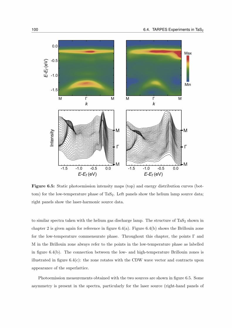
100 6.4. TARPES Experiments in TaS2
-1.5 -1.0 -0.5 0.0
Intensity
-1.0 -0.5 0.0M
M
M MΓ
Min
Max
-1.5
-1.0
-0.5
0.0
k
M MΓ
k
Γ
E-Ef (eV) E-Ef (eV)
E-Ef (eV)
M
M
Γ
-1.5
Figure 6.5: Static photoemission intensity maps (top) and energy distribution curves (bot-
tom) for the low-temperature phase of TaS2. Left panels show the helium lamp source data;
right panels show the laser-harmonic source data.
to similar spectra taken with the helium gas discharge lamp. The structure of TaS2 shown in
chapter 2 is given again for reference in figure 6.4(a). Figure 6.4(b) shows the Brillouin zone
for the low-temperature commensurate phase. Throughout this chapter, the points Γ and
M in the Brillouin zone always refer to the points in the low-temperature phase as labelled
in figure 6.4(b). The connection between the low- and high-temperature Brillouin zones is
illustrated in figure 6.4(c): the zone rotates with the CDW wave vector and contracts upon
appearance of the superlattice.
Photoemission measurements obtained with the two sources are shown in figure 6.5. Some
asymmetry is present in the spectra, particularly for the laser source (right-hand panels of

Chapter 6. Time- and Angle-Resolved Photoemission Spectroscopy of 1T -TaS2 101
figure 6.5). These asymmetries are caused by two effects. First of all, as is clear from figure
6.3, the experimental geometry means that photons from either source are incident at large
angles to the sample surface when looking at photoelectrons emitted near normal incidence,
so around the centre of the Brillouin zone. As the sample is rotated to look from one side
of the zone to the other, the angle of incidence of the XUV photons is not symmetric about
the surface normal. The optical constants can change rapidly, such that the absorption is not
symmetric about the zone centre. This angular variation is also polarisation dependent, which
is the second cause of the asymmetric spectra. The helium lamp is unpolarised, whereas the
laser source is p-polarised, leading to the differences in symmetry between the two spectra.
Despite the asymmetry, the laser source is able to reproduce the salient features of the
spectrum. The appearance of the Mott gap is indicated by the limited spectral weight at the
Fermi energy and the formation of the lower Hubbard band at around −0.2 eV. The sub-
manifolds associated with the structural distortions can be resolved, with the shadow bands
appearing at k = 0 (the Γ point). These bands are separated by a gap at the reconstructed
Brillouin zone boundary (the M point). All these features are in agreement with existing
photoemission data on TaS2 [28, 34, 172]. In light of this, the time-resolved measurements
are expected to produce reliable representations of the changes in band structure after pho-
toexcitation.
6.4.3 Time-resolved measurements
Time-resolved measurements of the photoemission spectrum were made as the phase transi-
tion occurs and the system evolves in response to excitation of TaS2 with a pump laser pulse.
The time-dependent energy distribution of photoelectrons is shown in figure 6.6, where the
response has been integrated across the entire Brillouin zone. The collapse of the Mott gap
is indicated by a loss of intensity below the Fermi energy, especially in the lower Hubbard
band, along with an increase of spectral weight above it. Following this prompt change, there
are oscillations in the intensity due to a rigid shift back and forth of the entire spectrum,
as shown in figure 6.6(b). These oscillations occur at the frequency of the CDW amplitude
mode and are connected to its coherent excitation. These features are all in agreement with
the earlier time-resolved studies [28, 37].
What separates this study from the previous ones is the ability to have momentum reso-

102 6.4. TARPES Experiments in TaS2
-0.3
-0.2
-0.1
0.0
0.1
Time (ps)
Min
Max
-0.5 0.0 0.5 1.0 1.5
Time (ps)
-0.5 0.0 0.5 1.0 1.5
0
10%
20%
30%
E-Ef (e
V)
∆(I
nte
nsity)
at Ef
Figure 6.6: Temporal behaviour of the electronic structure. (a) Map of photoelectron
intensity, integrated over the entire Brillouin zone, as a function of time before and after
photoexcitation. (b) Intensity changes at the Fermi level. Dots are experimental data, while
the blue line is a fit accounting for the onset and oscillatory decay of the electronic response.
The red dashed line is the non-oscillatory component of the fit.

Chapter 6. Time- and Angle-Resolved Photoemission Spectroscopy of 1T -TaS2 103
U1
-600 -400 -200 0 200 400
+200 fs
-100 fs
+60 fs
+200 fs
∆(I
nte
nsity)
Ef
LHB
E-Ef (meV)
Inte
nsity
x10
Inte
nsity
(a)
-100 0 100 200
EfLHBU1∆
(In
ten
sity)
(sca
led
)
Time (fs)
(b)
Figure 6.7: Evolution of the bands through the photoinduced phase transition. (a) The
top panel shows a high-resolution energy distribution curve (EDC) at the Γ point. U1 –
uppermost Umklapp band. LHB – lower Hubbard band. Ef – Fermi energy. The middle
panel gives EDCs before and after photoexcitation. The bottom panel shows differential
EDCs at 60 and 200 fs after photoexcitation. (b) Temporal evolution of changes at the Γ
point for three key energies.
lution and observe a large portion of the Brillouin zone. Of particular interest is the response
of the lower Hubbard band and the uppermost Umklapp band, where effects are found to
occur at different rates. Changes taking place at the Γ point are summarised in figure 6.7. As
shown in figure 6.7(a), spectral weight at the Fermi level and just above it appears promptly
and has begun to decay by 200 fs. On the other hand, around the uppermost Umklapp band
the intensity is suppressed, and this suppression is still growing 200 fs later. This difference
in behaviour can be seen more clearly in figure 6.7(b). Here, the intensity changes are plotted
as a function of time for the three key areas of the photoemission spectrum: at the Fermi
energy, at the lower Hubbard band, and at the uppermost Umklapp band.
From figure 6.7, then, there are clearly different timescales associated with the changes
at different positions in momentum and energy, which can be attributed to different physical
mechanisms. At the Fermi energy there is an increase in intensity brought about by the
melting of the Mott gap. This change is expected to be prompt, as it is connected to the
electronic phase transition. Indeed, its response time is equal to the pump-probe cross-
104 6.4. TARPES Experiments in TaS2
correlation time of 45 fs. The gap collapse also causes the loss of intensity at the lower Hubbard
band, and the same temporal response is seen there. At lower energies, in the shadow bands,
the response is slower. This is consistent with a reduction in spectral weight brought about by
unfolding of the band structure due to incipient relaxation of the coupled CDW and lattice
distortion. Such changes occur on structural rather than electronic timescales, hence the
slower response time.
Whilst one timescale dominates over the other at these three key regions, at different
energies and momenta the spectral changes are characterised by a mixture of the two. Figure
6.8 illustrates the temporal evolution of the differential photoelectron intensity at both the
zone centre and the zone boundary for a number of different energies. To separate the
contributions of electronic and structural processes, the data at earliest times were fitted in
the time domain using two timescales. The first is that of the prompt electronic response
of the system, limited by the instrumental response time; the second slower timescale is
associated with the onset of structural relaxation. The fit then takes the form
∆I(t) = A erf(t/w) +(e−t2/w2
)∗(Be(t−t0)/τ
). (6.4)
The first term represents the electronic response as an error function of width w, derived from
a step function convolved with the Gaussian pump-probe cross-correlation function, which
has a full width at half maximum of w = 45 fs. The second term represents the structural
response, where this time the cross-correlation is convolved with an exponential increase that
only begins to turn on at t = 0. The time constant τ for this exponential growth is equal to
half of the CDW amplitude mode period (ωAM ≈ 2.5THz). The resulting fits are given by
the solid lines in figure 6.8.
The relative contribution of the two components varies as the momentum is increased
from Γ to M, as can be seen by comparing the two panels of figure 6.8. This becomes more
apparent in figure 6.9(a), where the amplitudes of the electronic and structural fit components
across the Brillouin zone are displayed separately.
On electronic timescales, spectral intensity is lost at the peak of the lower Hubbard band
and transferred across the Fermi level. This corresponds to the creation of hot electrons and
the loss of the Mott gap. As seen in figure 6.9(a), this process is momentum independent,
indicating that the effects of the electron-electron interaction pervade the Brillouin zone.
Conversely, the structural response exhibits dispersion, with some important features

Chapter 6. Time- and Angle-Resolved Photoemission Spectroscopy of 1T -TaS2 105
-100 0 100 200 -100 0 100 200
LHB
U1
∆(I
nte
nsity)
At Γ point At M point
Time (fs) Time (fs)
Ef
Figure 6.8: Variation of dynamics over the full range of energies at the Γ (left panel) and M
points (right panel). Each trace represents the intensity change at a particular energy. Dots
are experimental data and curves are fits to a two-component model (see text). Key spectral
features are indicated by the shaded regions, where U1 is the uppermost Umklapp band, LHB
is the lower Hubbard band, and Ef is the Fermi energy.

106 6.4. TARPES Experiments in TaS2
-400
-1
0
1
Amplitude
Fast (electronic) response
Slow (structural) response
-200
0
kM
LHB
E-E
f (m
eV
)E
-Ef (
me
V)
U1
-400
-200
0
Γ
(a)
0
Str
uctu
ral
resp
onse
at E
f
kΓ
k (1)f k (2)f
M
(b)
Figure 6.9: (a) Spectral distribution of changes to band structure on electronic (top) and
structural (bottom) timescales. The purple lines indicate the lower Hubbarb band (LHB)
and uppermost Umklapp band (U1) peak positions in the low-temperature insulating phase.
The arrows indicate transfer of electronic spectral weight. (b) Amplitude of slow changes in
spectral intensity at the Fermi level. The arrows indicate the two Fermi wave vectors in the
high-temperature incommensurate phase.

Chapter 6. Time- and Angle-Resolved Photoemission Spectroscopy of 1T -TaS2 107
emerging from the lower panel of figure 6.9(a). Around k = 0, a negative amplitude for the
structural fit component in the Umklapp band indicates a partial loss of this band as the CDW
distortion relaxes and the zone unfolds. Furthermore, there is positive amplitude between the
low-temperature bands at the M point, signifying a softening of the CDW gap in this region.
Across the Brillouin zone, positive amplitude is concentrated above the lower Hubbard band
peak, implying that the band edge is shifting upwards in energy as the structure relaxes.
Figure 6.9(b) plots the amplitude of the structural fit component near the Fermi energy.
From this, it can be seen that the energy shift due to the relaxation is concentrated at the
Fermi wave vectors of the high-temperature incommensurate phase. So, photo-doping not
only melts the Mott gap, creating a transient metallic phase, but it also partially undoes
the low-temperature structural distortions, driving the system back towards the undistorted
high-temperature phase.
6.5 Summary
This chapter has built on the characterisation of the photoinduced phase of TaS2 undertaken in
chapter 5 by monitoring the temporal evolution of the electronic band structure in response
to excitation with light. This has been done using time- and angle-resolved photoelectron
spectroscopy with sub-50-fs time-resolution to separate the effects of electrons and lattice.
Additionally, the high photon energy used enabled a full investigation of the Brillouin zone
to be undertaken, expanding upon previous photoemission measurements [28].
At the earliest times of the phase transition, TaS2 is seen to become metallic through the
collapse of the Mott gap. At the same time, structural relaxation begins to occur, though its
slower onset shows that it is not the driving force behind the transient metallic state. Long-
range CDW order is retained in this phase, as shown by femtosecond electron diffraction
measurements [71] and as suggested by the results of chapter 5. However, the TARPES study
indicates that the effects of CDW-related backfolding of the Brillouin zone are at least partially
undone by photoexcitation, shifting the band edge up in energy towards the high-temperature
phase.
The ability to separate time and energy scales across momentum space afforded by
TARPES experiments is a crucial step in understanding the dynamics of strongly correlated
materials. In future, it should allow for the testing of theories of the electronic spectrum in

108 6.5. Summary
complex systems, as well as unveiling the interplay between their different degrees of freedom.
When combined with other spectroscopic techniques, such as those presented elsewhere in this
thesis, a more detailed and richer understanding of the physics of correlated materials begins
to emerge.

Chapter 7
Vibrational Excitation of Complex Materials
7.1 A New Approach
The photoexcitation technique used in the preceding chapters and, indeed, in the majority
of previous pump-probe experiments, relies on pumping the system with photons on the eV
energy scale. This energy couples directly to the electrons, creating hot carriers which then
interact with the other degrees of freedom, re-distributing the energy throughout the system.
It has also frequently been mentioned that the ground state of a complex material is deter-
mined by strong competition between many parameters, including phonons, electrons, and
magnetic interactions. Furthermore, many photoinduced phase transitions are accompanied
by structural changes, making the role of electrons and phonons in the transition somewhat
unclear. A natural question then arises: can a phase transition be initiated by driving phonon
excitations, without exciting the electronic structure? If light can be coupled to a lattice vi-
bration by making its frequency resonant with that of the phonon mode, this could help
elucidate the role of structural distortions in the phase transition.
This chapter will present some preliminary work on this approach. These ‘vibrational
control’ experiments were initially carried out in the manganites, although the technique
is now being extended to other materials, including organic Mott insulators and cuprates.
Tabletop techniques allow for investigations into the mid-infrared range, whilst free electron
lasers offer the opportunity to explore the role of much lower-energy excitations.
109

110 7.2. Manganites
La , Sr , Ca ,...3+ 2+ 2+
Mn , Mn3+ 4+
O2-
Figure 7.1: The ideal unit cell of an ABO3 perovskite. The A-sites are occupied by rare
earth ions at the corners of the cell. The B-sites are occupied by manganese ions. Oxygen
ions form an octahedral cage around the manganese ion.
7.2 Manganites
7.2.1 Basic properties
The manganites are a family of materials containing trivalent or tetravalent manganese ions
[186]. Many of them form in the ABO3 perovskite structure, illustrated in figure 7.1. In
this type of structure, the A-sites contain large ions, typically rare earth or alkaline earth
ions, such as Ca2+, La3+, or Sr2+, whilst the B-sites have a smaller ion of Mn3+ or Mn4+, or
some other transition metal for different oxide families, such as cuprates or cobaltites. The
O2− ions sit on the faces of the A-site cube, forming an octahedral cage around the central
manganese ion.
The manganese ions have an active d-shell, with five degenerate levels in the uppermost
3d manifold. When placed into the perovskite crystal structure, the crystal field lifts this
degeneracy, creating a lower-energy three-fold-degenerate t2g level and a higher-energy two-
fold-degenerate eg level. This crystal-field splitting, often referred to as the 10Dq splitting,
is typically of the order of 1 or 2 eV in manganites [187]. A sketch of the splitting is given in
figure 7.2.
There is a strong Hund coupling between the spins in manganites, which results in the
four electrons of the Mn3+ ion being in a state of maximum spin [188]. This produces the
configuration t32g↑eg↑, as shown in figure 7.2. This configuration is unstable to a Jahn-Teller

Chapter 7. Vibrational Excitation of Complex Materials 111
t2g
eg
Figure 7.2: Schematic representation of the d-level electronic structure for a Mn ion in
isolation (left) and in the presence of cubic (middle) and tetrahedral (middle) crystal fields.
Arrows indicate spins.
distortion of the lattice [189], in which the degeneracy of the t2g and eg levels can be lifted
and the overall energy of the system lowered. This can be viewed by considering the electron
orbitals: the t2g levels consist of dxy, dyz, and dzx orbitals, which point between the oxygen
anions, whilst the eg levels consist of dx2−y2 and d3z2−r2 orbitals, pointing towards the oxygen
anions. Then, for a distortion along the z-direction, the Coulomb energy of the d3z2−r2 orbital
is lowered due to the expansion along this axis. However, this increases the Coulomb energy
between the dx2−y2 orbital and the oxygen anions. For the Mn3+ cation, the dx2−y2 orbital
is unoccupied, so it becomes energetically favourable for the distortion to take place. This
effect is illustrated on the right-hand side of figure 7.2. In Mn 4+ ions, the eg levels are empty
and there is no Jahn-Teller effect.
Additional deviations from perfect cubic perovskite structure occur in the form of tilting
of the oxygen octahedra. The degree of tilting is dependent on the size of the A-site cation
[190], and is an important parameter for the properties of the manganites, as shall be seen
shortly.

112 7.2. Manganites
Interest in manganites grew dramatically in the 1990s after they were found to display
the colossal magnetoresistance effect [191–193]. Magnetoresistance describes the change in
electrical resistivity of a material under the influence of an external magnetic field. Ordinarily,
the resistivity increases when a magnetic field is applied, since the electron path is lengthened
by the additional force of the field. However, manganites show the opposite behaviour, with
the resistivity decreasing with increasing magnetic field. This negative magnetoresistance was
dubbed colossal due to the enormous size of the effect; resistivity changes of some nine orders
of magnitude have been recorded [193].
7.2.2 Phase transitions
From the preceding discussion, it is clear that the manganites are highly sensitive to the types
of ion used, the number of electrons in the system, and the departure from cubic structure
introduced by distortions. Indeed, the correlations between charge, lattice, spin, and orbital
degrees of freedom are very strong, and subsequently manganites display a range of interesting
phenomena. Moreover, they exhibit very rich phase diagrams as external parameters such as
temperature, pressure, chemical doping, and magnetic field are varied, with subtle changes
leading to dramatic alterations in the macroscopic properties.
Many different phases can be obtained by altering the chemical doping. By changing the
A-site ions to some new composition of the form A1−xA′xMnO3, the ratio between trivalent
and tetravalent manganese ions is shifted. This alters the magnetic state by changing the spin
from site to site, which can have a large impact on the conducting properties. The ground
state can include insulating and metallic ferromagnetic or insulating antiferromagnetic phases,
and may show charge and/or orbital ordering behaviour [187]. As an example of the variation
in behaviour, the phase diagram for La1−xSrxMnO3 as a function of temperature and chemical
doping x is shown on the left-hand side of figure 7.3, where an array of metallic and insulating
phases may be observed.
In addition to altering the number of holes at the manganese sites, chemical substitution
produces mismatch between the ionic radii at the A-sites, which can introduce strain. For
smaller A-site cations, the oxygen anions are pulled away from their ideal positions, distorting
the octahedra. This changes the Mn–O–Mn bond length and angle, and alters the electronic
bandwidth.

Chapter 7. Vibrational Excitation of Complex Materials 113
Figure 7.3: Properties of manganites. Left: phase diagram for La1−xSrxMnO3, taken
from [194]. PI, PM and CI denote paramagnetic insulating, paramagnetic metallic and spin-
canted insulating states, respectively. FI, FM, and AFM denote ferromagnetic insulating,
ferromagnetic metallic, and antiferromagnetic metallic states. Right: effect of pressure on
resistivity as a function of temperature in La0.79Ca0.21MnO3, taken from [195].
In manganites, conduction takes place by hopping of electrons from manganese site to
manganese site via intermediate oxygen sites in a ‘double-exchange’ mechanism [196, 197].
The effective hopping t between sites is proportional to cos θ, where θ is the angle of the
Mn–O–Mn bond. For large distortions, then, θ shrinks and the kinetic energy of the electrons
decreases, reducing the hopping and creating a tendency for insulating behaviour.
The bond angle, and, more importantly, the orthorhombic distortion of the manganites,
is often quantified through the geometric ‘tolerance factor’, defined as
Γ =dA–O√2dMn–O
, (7.1)
where dA–O is the distance between the A-site and the nearest oxygen ions, and dMn–O is the
shortest distance between manganese and oxygen ions [187]. An undistorted structure has
dA–O =√2 and dMn–O = 1, in units of the Mn–O distance, and hence has Γ = 1. As the
A-site ions shrink and the oxygens move away from their ideal positions, dA–O gets smaller
and Γ < 1, indicating a reduced Mn–O–Mn angle and thus a reduced hopping amplitude as
the electron orbital overlap decreases. The tolerance factor is minimised for a bond angle of

114 7.3. Pr1−xCaxMnO3
Figure 7.4: The properties of Pr1−xCaxMnO3. Left: phase diagram as a function of tem-
perature and doping x. PI, COI, CI, and FI are paramagnetic, charge-ordered, spin-canted,
and ferromagnetic insulators, respectively. AFI and CAFI are antiferromagnetic and canted
antiferromagnetic insulators. Right: structure of Pr1−xCaxMnO3, with the orthorhombic
distortion exaggerated for clarity.
90, when the hopping also vanishes [197, 198].
As well as being affected by doping, the tolerance factor can also be altered by applying
pressure. This changes the distortion of the structure, altering both the octahedral tilting and
any Jahn-Teller distortions which may be present. In turn, the bandwidth and the conducting
properties can be altered. The effect of pressure on resistivity is shown on the right-hand side
of figure 7.3 for La0.79Ca0.21MnO3. Here, the resistivity is quashed and the ferromagnetic
transition temperature, given by the peak in the resistivity curve, is shifted by increasing the
hydrostatic pressure.
7.3 Pr1−xCaxMnO3
Pr1−xCaxMnO3 (PCMO) is unique among the manganite family inasmuch as it has no in-
sulating phase for any temperature or chemical doping [193]. This is due to the small ionic
radius of the calcium cations, which produces a large distortion of the oxygen octahedra and

Chapter 7. Vibrational Excitation of Complex Materials 115
a tendency toward charge localisation. As a result, the tolerance factor Γ is small. The phase
diagram of PCMO is shown on the left of figure 7.4, while its structure is shown on the right.
In this diagram the tilting has been exaggerated for effect.
Despite of the lack of metallic behaviour with chemical doping, it is possible to induce an
insulator–metal phase transition by application of magnetic field [193] and external pressure
[199, 200]. Furthermore, at x = 0.3, there is a photoinduced metallic phase, which has been
characterised by large resistivity changes [201–203].
Given the existence of this photoinduced phase, the importance of the structural distor-
tions on the electronic properties, and the pronounced distortion present in this compound,
PCMO would seem to be a natural candidate for a vibrational control experiment. The con-
ducting properties rely on the structure, modulation of which by pressure drives the system
metallic. If the structure can be directly modulated using light, it may be possible to drive
the system into a conducting phase without excitation of the electrons, but by altering the
conducting pathways themselves.
Figure 7.5 shows the optical conductivity of PCMO between 10 and 100meV [204]. Three
modes are present at 23, 42, and 71meV, corresponding to three infrared active vibrational
modes of a cubic perovskite. They are identified as the Pr/Ca site external mode, the Mn–
O–Mn bending mode, and the Mn–O stretching mode, respectively [205]. The experiments
discussed in the rest of this chapter will focus on large-amplitude coherent excitation of these
modes in a bid to drive the system into a metallic state on ultrafast timescales.
7.4 Vibrational Control Experiments
7.4.1 Experimental setup
The experimental setup used for the vibrational control measurements is very similar to
that employed in the TaS2 measurements of chapter 5. Figure 7.6 illustrates the layout. A
Ti:sapphire laser operating at 1 kHz and 800nm central wavelength is split into two parts.
The larger part of the beam is fed into an optical parametric amplifier (OPA), whose design is
the same as that described in chapter 3. This OPA acts as the pump source. The signal and
idler outputs are spilt using dichroic mirrors and then recombined non-collinearly in a GaSe
crystal, where they interact to produce tunable mid-infrared light by difference frequency

116 7.4. Vibrational Control Experiments
Bending mode Stretching mode
Figure 7.5: Optical conductivity spectrum of Pr0.7Ca0.3MnO3 at 10K, taken from [204].
Also illustrated are bending and stretching modes of the Mn–O octahedra.
generation (DFG). The non-collinear arrangement allows for spatial filtering of the light,
minimising losses due to filters.
The DFG scheme is capable of producing radiation down to around 20µm (62meV) with
pulse energies of a few microjoule. This makes it ideal as a source to study the response of
the highest-lying stretching mode at 71meV. The pump light generated was then focussed
down onto a Pr0.7Ca0.3MnO3 sample with intensities of around 1mJ cm−2. A doping level
of x = 0.3 was used to coincide with studies of the photoinduced phase transition already
performed at that doping. Henceforth, the term PCMO will only refer to Pr0.7Ca0.3MnO3.
The sample was fixed onto a cryostat cold finger, allowing the temperature to be controlled
down to a few kelvin.
The second part of the main laser beam was passed into a second OPA, which could be
tuned between the visible and the infrared, just as in chapter 5; this constituted the probe

Chapter 7. Vibrational Excitation of Complex Materials 117
BS
OPA
Laser in GaSe
OPA
Figure 7.6: Schematic layout for the vibrational control experiment in PCMO. OPA –
optical parametric amplifier. BS – beam splitter. The orange circle represents the cryostat
cold finger, with the sample (black line) mounted at its centre. The grey-blue box is a delay
stage.
beam. Its delay relative to the pump beam was controlled with a delay stage, so that the
response to mid-infrared excitation could be mapped out in time.
The pump beam was chopped using a mechanical chopper wheel and reflectance changes
to the probe beam were recorded by lock-in detection, all as in chapter 5.
7.4.2 Experimental results
The PCMO sample was held at 30K and pumped with light resonant to the 71meV stretching
vibration. The reflectance was measured as a function of pump-probe time delay and is shown
in figure 7.7(a). A prompt change in reflectance is observed on arrival of the pump, which
decays after around 1 ps to a long-lived phase lasting for hundreds of picoseconds, as indicated
by the constant change in reflectance at long times. No dependence on pump polarisation
was observed in any of the measurements. The reflectance changes observed are qualitatively
similar to those seen after excitation at 1.55 eV, with the same dynamics and development of
a meta-stable state. In the equilibrium insulating state of PCMO, the insulating gap has size
∆ = 180meV [204]. Crucially, then, the 1.55 eV pump energy is far in excess of the insulating
gap size, whereas 71meV lies below it. This suggests that an ultrafast response that is similar
in nature to that formed by above-gap excitation may be induced by pumping below gap.
In order to characterise the photoinduced phase, the reflectance changes were measured
across a range of probe energies for the same pump intensity. Figure 7.7(b) summarises

118 7.4. Vibrational Control Experiments
-2 -1 0 1 2 3 4 5
0.00
0.02
0.04
0.06
0.08(a)
R
/R
Time (ps)
0.80 0.85 0.90 0.95 1.00 1.05
-0.03
-0.02
-0.01
0.00
R/R
Probe energy (eV)
(b)
Figure 7.7: Reflectance changes for PCMO after photoexcitation with mid-infrared radi-
ation. (a) Reflectance changes as a function of time after excitation at 71meV, measured
at 0.99 eV (1250 nm). (b) Probe energy dependence of the reflectance changes 1 ps after
excitation with 71meV pulses.

Chapter 7. Vibrational Excitation of Complex Materials 119
the results obtained in the near-infrared between 1.05 and 0.8 eV, showing the reflectance
changes 1 ps after excitation at 71meV. Additional spectrally resolved measurements were
also obtained at higher probe energies by Rini et al. [206]. Overall, a decrease in reflectance is
seen for energies between 0.8 and 2 eV, whilst an increase occurs for higher photon energies.
This spectrum is consistent with previous results obtained for the photoinduced insulator–
metal transition in PCMO [203]. In that study, it was shown that above-band-gap excitation
and application of a magnetic field can induce the same spectral features, characterised by a
decrease in reflectivity between 0.5 and 1.9 eV and an increase above it. This was attributed
to a collapse of the insulating gap present at equilibrium. The direct correlation between the
results of figure 7.7(b), combined with those of Rini et al. [206], and the earlier optical study
implies that a metallic state is formed promptly as a result of photoexcitation resonant with
a lattice vibration of the system.
The response of PCMO to mid-infrared pumping was investigated further by Rini et al.
by tuning the pump wavelength across the resonance feature [206]. The reflectance change
is maximum when the pump wavelength is resonant with the Mn–O stretching mode, and
vanishes as the wavelength is tuned away from it. Conductivity measurements were also
carried out by measuring the resistance between gold electrodes fixed to the surface. These
showed a five-order-of-magnitude increase in conductivity immediately after excitation, with
the change decreasing as the pump was tuned away from resonance [206]. All of this provides
further support for the notion of a vibrationally induced ultrafast insulator–metal phase
transition.
The results presented in figure 7.7, together with those of Rini et al., show that reso-
nant excitation of the Mn–O phonon mode at 71meV in PCMO initiates a transition to
a meta-stable conducting phase. This happens on femtosecond timescales and persists for
nanoseconds. Importantly, this transition does not excite electrons, since the photon energy
is below gap, so that the electrons remain in their ground state. Furthermore, since no ther-
mal metallic phase exists for PCMO for any value of doping x, as indicated by figure 7.4,
the effect cannot be caused by simple laser heating. Rather, it appears that coherent mod-
ulation of the tolerance factor, induced by exciting a vibrational mode of the system, leads
to dramatic changes in the electron hopping probability. This demonstrates an alternative
mechanism for ultrafast phase transitions in correlated materials, highlighting the important

120 7.5. Studying Resonant Effects
role played by structural effects in these systems.
7.4.3 The next steps
This first experiment demonstrates the possibility of vibrational excitation for driving ul-
trafast changes in correlated materials. The approach opens the way to understanding the
importance of the lattice in a host of interesting and elusive problems, including colossal
magnetoresistance and high-temperature superconductivity, where phonons are expected to
play a crucial part. The coupling between spin and lattice degrees of freedom also makes
the manipulation and control of magnetic states an attractive prospect. Depositing energy
directly into specific lattice modes and bypassing the electrons may provide fresh insight
into the behaviour of many types of complex material, highlighting the role of the lattice in
determining the electronic properties.
However, in order to understand all these effects, there are a few points to consider in
moving forward. First, what is the importance of specific modes? Can driving different modes
in the system have the same effect or does it differ, and why? Comparing the effects for dif-
ferent modes would help elicit information on the conduction mechanisms in the material and
on the role of the structural distortions in the electronic properties more generally. Further-
more, what is the role played by the electric field of the light pulse? What are the sub-cycle
distortions caused by the field doing to the electronic structure? These are more long-term
goals, but attempting to address them will form the remainder of this chapter.
7.5 Studying Resonant Effects
7.5.1 Laboratory limitations
The measurements carried out in section 7.4 used tabletop sources to produce the light re-
quired for studying the highest-lying mode in PCMO. Somewhat serendipitously, the wave-
length range afforded by difference frequency generation covers this mode, but stops at around
20µm (62meV), making an exploration of the other modes impossible with the available non-
linear optical techniques.
In order to understand the role played by specific structural distortions in ultrafast phase
transitions, it is important to be able to study the effects of different modes. This can be

Chapter 7. Vibrational Excitation of Complex Materials 121
achieved by performing experiments in materials which have modes at higher frequencies or
by using different sources of light to access lower-frequency modes.
The first route has been explored for the organic one-dimensional Mott insulator (BEDT-
TTF)-F2TCNQ. This compound has phonon modes at 6µm and 10µm, which are expected
to affect the electronic bandwidth of the system in different ways by altering the electron
orbital overlap. By driving these two modes with mid-infrared light from table-top sources, a
collapse of the Mott state was found for one mode but not the other, highlighting the different
role played by structural distortions in the two cases [207].
However, as can be seen for the manganites in section 7.3, such systems with accessible
modes cannot always be found. Free electron lasers offer a way around the limitations of
traditional nonlinear techniques, opening up the possibilities for examining other modes of
the system.
7.5.2 Free electron lasers
The free electron laser (FEL) is capable of producing tunable radiation over a broad range
of wavelengths, from the far-infrared up to X-rays, using a high-energy electron beam as
a lasing medium [208–210]. The free electron laser at the superconducting electron linear
accelerator with high brilliance and low emittance (FELBE) located at Forschungszentrum
Dresden-Rossendorf, Germany, is an FEL operating in the far- to mid-infrared regions [211].
A schematic of the FEL is shown in figure 7.8. The electron beam is generated by a thermionic
electron gun and then accelerated by a superconducting linear accelerator. The undulator is
a series of magnets whose field direction alternates from section to section, as illustrated in
figure 7.8. The magnetic field moves the electrons back and forth in a direction perpendicular
to the undulator axis, causing the electrons to emit radiation with a wavelength determined by
their energy and the undulator period and gap size. The wavelength of the infrared radiation
can thus be tuned by adjusting the undulator gap, for a given period.
The undulator sits in the centre of a resonator consisting of two mirrors whose separation
is fixed by the repetition rate of the electron beam, set at 13MHz. The resonator is tuned to
maximise the power output of the FEL. There are two undulators in use at FELBE, which
provide almost continuous coverage from 4 to 250µm [212, 213]. The spectral width of pulses
produced by FELBE is typically ∆λ/λ 6 2%, depending on the wavelength desired. The

122 7.5. Studying Resonant Effects
Beam dump
Undulator
Superconductingaccelerator
Electroninjector
Mirror Mirror
IR beam
Figure 7.8: Schematic layout of the FEL at FELBE.
pulses are Fourier limited, putting their duration in the range of several picoseconds.
Thus FELBE provides a source of tunable narrowband infrared radiation across a range of
wavelengths, making it suitable for studying the role of different phonon modes in vibrational
control experiments in PCMO and any number of other complex materials. While it offers
narrower bandwidth pulses, which would allow for better understanding of the selectivity of
the effects, this naturally comes at the expense of the pulse duration, which is lengthened
from the femtosecond to picosecond timescales.
7.5.3 Experiments at FELBE
While excitation of the stretching mode at 71meV showed an ultrafast insulator–metal phase
transition, it is desirable to try to understand what the importance of this particular distortion
is. To this end, the FELBE free electron laser could be used to try to excite the two other
lower-frequency modes at 23 and 42meV, corresponding to the Pr/Ca site external mode and
the Mn–O–Mn bending mode, respectively. Since conduction in manganites is supposed to
take place via double-exchange hopping between manganese and oxygen sites, the bending
mode is expected to play an important role in the transport properties, and so an effect
similar to that observed for excitation at 71meV should be seen. However, the lowest-lying
external mode does not affect the tolerance factor, leaving the Mn–O bond angle and length
unchanged, but moving the Pr/Ca ions relative to the Mn–O octahedra instead. As such, the
response is anticipated to be quite different when exciting this mode.
An important technical challenge to overcome in these experiments is concerned with the
repetition rate of the FEL. The mid-infrared pulse train has a frequency of 13MHz, giving
a pulse separation of some 77 ns. This is not desirable, since the meta-stable state found in

Chapter 7. Vibrational Excitation of Complex Materials 123
Ge
FEL in(13 MHz)
Laser(1 kHz)
FEL out(1 kHz)
0.6
0.2
0.4
0.0-400 -200 0 200 400
Am
plit
ude (
V)
Time (ns)
-600 -400 -200 0 200 400
0.02
0.01
0.00
-0.01
Figure 7.9: Using the optical switch to change the FEL repetition rate. Left: schematic
diagram of the switch inputs and outputs. Right: oscilloscope trace showing reflected FEL
pulses. The switching laser arrives at 0 ns. The inset shows the full scale of the switched-out
pulse for comparison with the unswitched pulses.
the laboratory experiments lasts for some nanoseconds before returning back to equilibrium.
Furthermore, the average power of the FEL at the wavelengths of interest is typically on the
order of several watts, meaning the laser could potentially heat the sample up. While there is
no thermal metallic phase, so that heating is not expected to produce conducting behaviour,
the effects of heating with the laser may suppress any transient effects it also induces. As
such, it is desirable to first turn down the repetition rate of the FEL to something much
lower, increasing the inter-pulse separation and reducing the average power.
This is achieved by using an optical switch, based on laser-generated plasma in germanium
[214]. The FEL beam is incident at Brewster’s angle onto a germanium plate, such that it
is transmitted with minimal reflection. A Nd:YAG amplified laser operating at 1 kHz and
1064 nm is focussed onto the germanium, where it generates an electron-hole plasma. For a
sufficiently high plasma density, the optical properties are altered so as to make the germanium
reflecting for the FEL. Since the electrons and holes eventually recombine, the effect is only
transient; a decay constant of 590 ps has been measured [214]. This means that if the FEL
arrives immediately after the Nd:YAG laser pulse, it will be reflected, while for times before
and soon after the Nd:YAG pulse, it will be transmitted. Since the laser has a repetition
rate of 1 kHz, the reflected pulses will also have a 1 kHz repetition rate, with the remaining
pulses blocked after passing through the germanium. This process is shown in figure 7.9.
Also shown in this figure is an oscilloscope trace recorded on a HgCdTe detector, sensitive to

124 7.5. Studying Resonant Effects
the mid-infrared wavelengths of the FEL. Ideally, only one pulse would be switched out by
the laser; in practice, the plasma is still dense enough to allow for partial switching of some
successive pulses. However, as can be seen from the figure and its inset, the ratio between
the initial switched pulse and all other pulses is very large, so that the effect of these residual
pulses is significantly smaller.
With the switch operational, the FEL repetition rate can be reduced to match the 1 kHz
Nd:YAG laser. While the unswitched pulses are not fully suppressed, a contrast ratio of
400:1 for switched to unswitched pulses was found during the experiment. The Nd:YAG laser
can also be used to probe the reflectance changes of the PCMO sample following vibrational
excitation.
A schematic of the experimental layout for the FEL experiments is shown in figure
7.10. The FEL beam was first sent through a polarisation rotator, consisting of a rotat-
able periscope. This was designed to optimise the polarisation of the FEL for the optical
switch. The unswitched FEL pulses were transmitted through the germanium and blocked
by a beam dump. A vacuum chamber similar to that used in chapter 5 was used for the
FEL measurements. This design was chosen rather than a more conventional cryostat since
it allowed for much smaller focal length optics to be used; this meant that greater pump
intensities could be achieved. The Nd:YAG probe beam was made collinear with the pump
by passing it through the back of the final pump focussing parabolic mirror. This was neces-
sary as the short focal length mirror crowded the sample. The intensity of the probe beam
was monitored using a silicon photodiode, and changes to the reflectance of the sample were
measured using lock-in detection. The whole optical table could be enclosed with plastic
and purged with nitrogen, which was important to prevent losses of the infrared light due to
absorption by water in the air.
7.5.4 Experimental results
As a first feasibility test for using the FEL to drive vibrational excitations, the wavelength
was tuned to 17.4µm (71meV) to try to repeat the laboratory measurements of section
7.4. The wavelength was then tuned down to 29.4µm (42meV), resonant with the bending
mode of PCMO. For these initial explorations, the measurements were performed at room
temperature, with the intention of cooling down to low temperatures after ironing out any

Chapter 7. Vibrational Excitation of Complex Materials 125
BS
Polarisation
rotator
GeBD
FEL in
Laser in
Figure 7.10: Schematic layout for the FELBE experiments. BS – beam splitter. Ge –
germanium. BD – beam dump. The orange circle represents the cryostat cold finger. The
sample (black line) is mounted to it and can be rotated about an axis perpendicular to the
page. The blue-grey box is a delay stage and the light blue box represents the vacuum
chamber.

126 7.5. Studying Resonant Effects
technical issues with using the FEL as a pump source.
The FEL was focussed down to a spot diameter of approximately 300µm, as measured
with a Spiricon infrared camera. The upper limit of intensity for the FEL pulses after the
optical switch was estimated as 200µJ cm−2 for the 17.4µm light, and 820µJ cm−2 at 29.4µm.
The low pulse energies make an accurate determination of the beam intensity at the sample
difficult at present, though schemes for calibration are in progress.
The preliminary results obtained by pumping PCMO at 17.4µm are displayed in figures
7.11(a) and (b). Despite the noise level, a change in reflectance is observed upon arrival of
the FEL pump pulse. The probe laser has a pulse duration of ≈ 20 ps, meaning the resulting
temporal profile is somewhat different to that observed with the femtosecond sources, although
the pump still initiates long-lived reflectance changes. The magnitude of the signal measured
100 ps after excitation shows a roughly linear dependence on the pump intensity. Despite the
low intensity achieved with the FEL, a photoinduced response is found, making the FEL a
viable source for investigating phonon-induced effects.
The wavelength was then tuned to 29.4µm; the first results obtained are shown in figures
7.11(c) and (d). As is the case at 17.4µm, a reflectance change is observed upon excitation
by the FEL, leading to a long-lived state. The signals obtained at this wavelength are noisier
than those found at the shorter wavelength due to FEL instabilities. However, it is still
possible to differentiate the response before and after the pump arrives. This represents the
first response from driving the bending mode in this compound.
7.5.5 Further measurements
The results presented from the experiments at FELBE represent the first investigations using
this source to study time-dependent phenomena in solids. Much is still to be done to improve
the system and understand the nature of the photoinduced dynamics. A better measure for
the intensity of the pump pulses is required; currently a scheme using HgCdTe detectors is
being implemented. Improvements in FEL stability and optical switch efficiency should also
increase the pulse energy and improve the signal-to-noise ratio.
Future measurements will require the cryostat to be used, reducing the temperature of
the sample to that used in earlier investigations. This is necessary to optimise the phonon
spectrum, reducing broadening introduced by thermal effects. It also allows for a more direct

Chapter 7. Vibrational Excitation of Complex Materials 127
-150 -100 -50 0 50 100 150
-0.010
-0.005
0.000
R/R
(%)
Time (ps)
(a)
0 50 100 150 200
-0.03
-0.02
-0.01
0.00
0.01(b)
R/R
(%)
Pump intensity ( J cm-2)
-150 -75 0 75 150-0.010
-0.005
0.000
R/R
(%)
Time (ps)
(c)
0 200 400 600 800
-0.015
-0.010
-0.005
0.000
0.005(d)
R/R
(%)
Pump intensity ( J cm-2)
Figure 7.11: Reflectance changes for PCMO after photoexcitation with FEL radiation. (a)
and (b): ∆R/R as a function of time and intensity after excitation at 17.4µm. (c) and (d):
∆R/R as a function of time and intensity after excitation at 29.4µm.

128 7.6. Field-Resolved Effects
comparison with the laboratory experiments. The tunable narrow bandwidth radiation offered
by the FEL means that future experiments should also focus on exploring the resonant nature
of the phonon-induced effects in a bid to understand the role of the structural distortion in
controlling the conducting properties. The unique characteristic of the FEL is its ability to
explore all three main phonons, so that a comparison of the different vibrations is possible.
This is important for any future understanding of the nature of ultrafast vibrationally induced
phase transitions.
7.6 Field-Resolved Effects
Section 7.4.3 proposed two directions for the field of vibrational control. The first, the explo-
ration of other modes and their role in controlling the electronic bandwidth, was discussed in
section 7.5. The second will be briefly discussed in this section.
The idea behind this proposal is to elucidate the importance of the driving electric field
when exciting vibrational modes of a complex material. Since the light couples to a structural
distortion, it is expected that the field of the pulse may be important to the process as it
modulates the ionic bonds. However, the precise nature of the structural modulation remains
to be seen.
While DFG is capable of producing infrared radiation resonant with lattice vibrations,
this radiation is incoherent in nature, in that the relationship between the carrier phase and
the pulse envelope is not well defined from pulse to pulse. This means that for each pulse in
the train, the electric field is slightly different and any information concerning the field is lost
as the signal is averaged over many pulses.
The carrier–envelope (CE) phase measures the offset between the peak of the electric field
and the peak of the pulse envelope. A change in CE phase from pulse to pulse represents
the slip of the carrier wave through the pulse envelope. In general, the CE phase evolves as
optical pulses propagate through a dispersive medium, where the phase and group velocities
are different [215]. This process occurs in mode-locked laser systems, meaning that their CE
phase is not stabilised. Instead, it varies by a fixed amount ∆ϕCE for each successive pulse.
This process is sketched in figure 7.12. If the CE phase was locked for each pump pulse then
the driving electric field would always look the same and phase effects may become apparent
when dealing with certain phenomena.

Chapter 7. Vibrational Excitation of Complex Materials 129
Df 2Df
t
Figure 7.12: Illustration of the carrier-envelope phase evolution from pulse to pulse. The
phase offset between pulses changes by an amount ∆ϕ.
Techniques exist to stabilise the CE phase of mode-locked laser systems, although these
all rely on active feedback mechanisms to correct for the group velocity mis-match in the
lasing medium [216]. However, passive stabilisation is also possible using OPAs.
In an OPA, a pump beam amplifies a signal beam, generating an idler beam in the process,
as described in chapter 3. It has been shown elsewhere that in parametric amplification the
phase of the signal wave is preserved while the beam is amplified [74, 217]. Furthermore, the
relationship between the phases ϕ of the pump, signal, and idler is given by
ϕI = ϕP − ϕS − π/2, (7.2)
where I, S, and P represent idler, signal, and pump respectively [217]. If the pump and
signal originate from the same laser source then their phases are locked and are related by
ϕP = ϕS + ∆ϕ, where ∆ϕ is constant. From equation (7.2), then, it follows that the idler
phase is constant regardless of any CE-phase instability of the laser. This principal has been
applied to generate phase-stable infrared light using different frequency components of the
same broadband pulse [218].
If two OPAs are driven by the same laser source, it follows that the mutual phase rela-
tionship between the signals of the two OPAs should be locked in a similar way to the pump
and signal of a single OPA. Then if the signal beams from each OPA are used as the pump
and signal in a DFG process, the idler generated from them should have a constant phase
for every pulse. This would provide a source of tunable mid-infrared light, as described in
chapter 3, except with CE-phase-stabilised pulses.
Such a scheme was employed to generate CE-phase-stable light by DFG in GaSe. The
resulting mid-infrared radiation was then detected using electro-optic sampling in a second

130 7.6. Field-Resolved Effects
-600 -400 -200 0 200 400 600
-0.75
-0.50
-0.25
0.00
0.25
0.50
0.75
1.00
Elec
tric
field
(a.u
.)
Time (fs)0 10 20 30 40 50
0.0000
0.0001
0.0002
0.0003
Mag
nitu
de
Frequency (THz)
Figure 7.13: A carrier-envelope phase stable pulse generated by DFG between two OPAs.
The dashed red lines represent a Gaussian envelope with FWHM ≈ 300 fs. The Fourier trans-
form spectrum is shown on the right. The central frequency is 25.5THz and the bandwidth
is ∆ν = 3THz.
GaSe crystal, using the same apparatus described in chapter 4. This field-resolved detection
of the electric field serves as proof of its phase stability: if the CE phase were not stabilised
then the field would slip through the envelope and appear slightly different for each pulse,
and the effect of averaging over successive pulses would wash out any field-related effects,
leaving only an effect characterising the pulse envelope.
Pulses were generated with typical energies of 0.5 to 2µJ for wavelengths between 10 and
18µm. Figure 7.13 shows a CE-phase-stable pulse generated at 11.8µm (25.5THz). The
stability of the CE phase offset was found to drift slowly over timescales of about an hour,
but can be corrected by introducing fused silica wedges into one of the OPA paths before the
difference frequency mixing takes place [219].
CE-phase-stable light generated in this way is expected to facilitate the study of field-
resolved effects in vibrational control experiments. Currently, investigation is underway in
applying these mid-infrared pulses to manganites, where the presence or absence of field-
induced effects should reveal important information about the phonon-induced phase tran-
sition [220]. Furthermore, their application to organic compounds, where work has already
been carried out using non-stabilised pulses, should demonstrate interesting phase-dependent

Chapter 7. Vibrational Excitation of Complex Materials 131
effects as the electron wavefunctions are coherently modulated across the molecule [207].
7.7 Summary
This chapter has tried to offer a brief overview of an emerging new field of ultrafast science, in
which light is coupled directly to structural modes of a system without electronic excitation,
rather than putting energy directly into the electronic degree of freedom. A first set of exper-
iments showed that it is possible to induce an insulator–metal phase transition by resonant
excitation of a stretching mode in a manganite system, presenting exciting new opportuni-
ties for understanding the important effect the lattice can have on influencing the electronic
properties. The use of FELs can open up the available spectrum for resonant excitation,
allowing the role of different modes to be explored across a range of different structures. At
the same time, the generation of CE-phase-stable pulses will allow field-dependent effects to
be monitored as the structure is modulated.
Subsequent to the first experiment in PCMO, other measurements have shown vibra-
tionally induced melting of charge order [221], control of the Mott criterion in organic insula-
tors [207], the generation of coherent phonons [220], and the creation of a transient supercon-
ducting phase in a doped cuprate [222]. The ability to initiate ultrafast dynamics by coupling
to phonons rather than electrons offers much promise in untangling the role of different de-
grees of freedom in strongly correlated materials and will become an important means to
understand a variety of problems, from magnetic and electronic ordering to high-temperature
superconductivity.

Chapter 8
Conclusion and Future Directions
8.1 Overview
This thesis has used a variety of ultrafast spectroscopic techniques to understand and char-
acterise photoinduced effects in complex materials. An understanding of the response of a
system across a range of energies is essential to determining its properties, be it an equilibrium
state or a transient photoinduced phase. Photoexcitation of solids enables the interactions of
different components to be separated, making ultrafast effects an important element of any
material study. In addition, understanding these effects can lead to control of them, which has
many potential technologically important applications. The broadband spectroscopic studies
presented in this work have combined photon energies from 1meV up to 20 eV as ultrafast
probes of the transient state of TaS2 induced by light at 1 and 1.5 eV. Meanwhile, the prin-
cipal of vibrational control in manganites was introduced, which demonstrates a new way to
understand and control the lattice in a variety of problems.
8.1.1 Tantalum disulphide
The photoinduced phase of 1T -TaS2 was explored using two approaches: broadband optical
spectroscopy to study the collective response of the system, and angle-resolved photoemission
spectroscopy to understand the single particle behaviour and electronic band structure. The
results of these investigations were described in chapters 5 and 6, respectively.
A time-resolved THz time-domain spectroscopy system was developed to allow for field-
133

134 8.1. Overview
resolved studies at the lowest energies. By preserving phase information in the pulses, a
direct reconstruction of the optical properties of a solid is possible as they evolve in response
to photoexcitation. This reveals information on long-range transport properties and can
also illuminate the response of phonon modes, allowing for explicit observations of both
electronic and structural effects in time in a single measurement. In TaS2, the complex
optical conductivity was recovered as a function of time. It was found that the melting of
the Mott gap leads to an increase in low-frequency conductivity, although not to the value
found at the thermal phase transition. Additionally, transient asymmetries were observed in
the phonon resonances, suggesting a coupling between these low-energy structural modes and
a higher-energy electronic excitation.
These low-frequency techniques were complemented by additional higher-frequency ap-
proaches. The output of a near-infrared optical parametric amplifier was extended into the
mid-infrared region using nonlinear optical techniques. This provided a femtosecond source of
probe light over a broad energy range. Whilst it lacks the phase information afforded by THz
spectroscopy, it reveals a lot about coherently generated phonons and about the dynamics
in a region not normally covered in pump-probe spectroscopy. Studies of the photoinduced
reflectance changes in the mid-infrared to visible regions revealed the excitation of the charge
density wave amplitude mode at 2.4THz. This suggests that the charge density wave distor-
tion is only partially undone by photoexcitation, in agreement with earlier studies [28, 71].
Moreover, the reflectance revealed the emergence of a new broad resonance at 155meV. Given
the strong electron-phonon coupling present in this material, this feature was interpreted as
a polaron band.
These two methods can characterise the dynamical behaviour of photoinduced phases
across a broad region of the spectrum, allowing for insight into ultrafast processes in enor-
mous detail. In addition, a time- and angle-resolved photoemission spectroscopy system was
developed, using high harmonic generation to produce photons at 20.8 eV with 50 fs resolu-
tion. Such a system enables the single particle response to be studied, capturing the dynamics
of electrons with momentum specificity, and mapping out the evolution of the band structure
after photoexcitation across large regions of the Brillouin zone. By studying the earliest times
of the photoinduced phase transition in TaS2, the collapse of the Mott gap could be directly
observed. Concomitantly, structural relaxation was seen to occur on timescales connected to
Chapter 8. Conclusion and Future Directions 135
the charge density wave, indicating a partial unfolding of the Brillouin zone back towards the
undistorted higher symmetry phase.
Bringing all these elements together presents a clearer view of the photoinduced phase
of TaS2. This phase is found to be qualitatively different from any of the thermal phases:
the Mott gap is lost and conductivity is found to increase, though it remains lower than
in the equilibrium metallic phase; the charge-density-wave structural distortion relaxes, but
only partly, with the symmetry of the low-temperature phase remaining unchanged; and the
transport properties are strongly polaronic, with a polaron band appearing at 155meV.
8.1.2 Vibrational excitation
Although the majority of the work presented in this thesis is connected to probing techniques,
a new type of pumping technique was introduced in chapter 7. This chapter dealt with the
idea of vibrational excitation, in which light is directly coupled to the structural modes of
a complex material, rather than the electronic excitations. A first set of experiments was
presented, in which an insulator–metal phase transition was initiated by modulation of a
stretching vibration in a perovskite manganite. This result opens up a new field of ultrafast
phase transition, in which electrons are left in their ground state but the lattice is excited. This
offers the potential to understand and control a number of processes in strongly correlated
electron materials where the lattice plays an important role in the electronic properties.
Following on from this, the potential application of FELs was described, accompanied by
some preliminary findings. The aim of these continuing measurements is to investigate other
phonon modes in the system and understand the role they play in controlling the conducting
properties. Finally, the generation of carrier–envelope phase stable radiation was introduced
and demonstrated. This may reveal new field-induced effects in complex materials, which
have hitherto been unobservable.
8.2 Looking Ahead
8.2.1 Tantalum disulphide
While the spectroscopic techniques presented in this thesis cover a broad spectral range and
go a long way towards characterising the salient features of the photoinduced phase of TaS2,

136 8.2. Looking Ahead
there is still room for further exploration.
Broadening the THz spectrum beyond 2.8THz would provide a more complete study of
the structural modes of TaS2, including the anomalous mode identified at 6.2THz, which
is believed to be connected to both structural and electronic changes at the thermal phase
transition [60]. At higher frequencies, a finer selection of probe wavelengths would yield more
detailed information on the polaron band, which may be connected to the loss and recovery
of the Mott gap.
There a number of additional investigations which may offer further information on the
photoinduced phase. Few-femtosecond pulses could help further differentiate the electronic
and structural processes in the photoinduced phase of TaS2, where the melting of both Mott
and charge-density-wave gaps cannot be distinguished with longer pulses. Also, tuning of
the pump photon energy could test the proposal of Perfetti et al. [28] that the photoinduced
phase transition originates from electronic temperature effects.
8.2.2 Vibrational excitation
The field of ultrafast vibrationally induced phenomena is still very fresh and offers many
possibilities for studying condensed matter systems. Going forward, it will be important to
start applying the kinds of spectroscopic technique used in this thesis to characterise the
phases induced by driving structural effects. This is important not only to understand their
behaviour but also to compare it to transient phases induced by electronic excitations and
look for differences between the two. This will help in understanding the competition between
electrons and lattice and how this determines the macroscopic properties of the system. Us-
ing photoemission spectroscopy will play a key role in this process, since it provides direct
measurements of the band structure which can be compared easily to theoretical predictions.
In terms of the initial measurements presented at the end of chapter 7, there is clearly much
still to be done. The FEL experiments are still in an early stage of development. However, if
successful, these measurements promise to provide much insight into the role of different types
of structural excitation in influencing the electronic properties of materials. Furthermore, the
effects of carrier–envelope-phase-stable radiation in these transitions needs to be considered,
since it offers some interesting prospects for new phases and coherent control.
Many new effects are being observed using vibrational excitation [220, 221], including con-

Chapter 8. Conclusion and Future Directions 137
trol of Mott insulators [207] and the induction of cooperative phases such as superconductivity
[222]. The real challenge now is to start characterising and understanding these states on a
number of different levels. This will require the marriage of ultrafast spectroscopic techniques,
such as those presented here, and these new methods for excitation and control.
8.2.3 Further afield
As developments in ultrafast technology continue apace, the condensed matter scientist is
increasingly spoilt for choice in the number of tools at his or her disposal. The field of ultrafast
science is constantly expanding into new territory, as pulses get ever shorter and the available
energy scales expand. These advances usher in fresh promises in terms of understanding the
behaviour of matter.
Two questions lie at the heart of this progression: what does light reveal about the different
phases of materials, and can light be used to control these states and to create new ones?
Controlling material properties has been a long-standing goal of solid state physics, and using
pulses of light has opened up avenues for transient and switchable behaviours unattainable
with more traditional techniques. Future possibilities include the control of magnetism or
superconductivity; if light can be used to coherently control the spin state of a lattice, or
generate macroscopic condensed states, then this would pave the way for a variety of exciting
technological applications.
The introduction of new spectroscopic techniques to the realm of the ultrafast is important
for the future characterisation of these controlled states and also to the broader understanding
of complex materials. The methods used in this thesis are making great strides towards this,
but it is necessary to bring other advancements into play.
Much as Muybridge’s images of horses and Victorian women were able to capture the
motion of everyday objects, so now are femtosecond X-ray and electron diffraction techniques
on the verge of capturing the motion of atoms [223]. Continuing improvements in free electron
lasers also promise snapshots of atomic motion on the shortest timescales and of the smallest
and most complex structures [224, 225]. Such developments bring the advent of the ‘molecular
movie’ ever closer, enabling direct observations of lattice dynamics as phase transitions take
place. Ultrafast X-ray techniques also bring the ability to understand electron spin and orbital
dynamics [27, 226], which are vital to the understanding of magnetic phenomena.

138 8.3. Final Remarks
It is also important to understand the electronic dynamics, as discussed in this thesis.
Time-resolved photoemission is a powerful tool for doing this, though it is still in its infancy.
The band structure measurements it provides can serve as a basis for theories of complex
materials and photoinduced phenomena which are still poorly understood. Moreover, as
pulses shrink down to the attosecond regime, the ability to observe charge transfer processes,
unveiling the precise motion of electrons through a material, is fast approaching [25, 182].
Ultimately, the combination of direct structural characterisation and a full determination
of the optical properties will provide a rigorous and comprehensive view of all aspects of the
dynamics of many intriguing materials. This deep understanding will also be important when
considering control and optimisation of their properties. Ultrafast spectroscopies are vital
for the study of all manner of materials, from low-dimensional organic compounds, to high-
temperature superconducting cuprates and pnictides, where the complex interplay between
different degrees of freedom leads to exciting yet elusive behaviour.
8.3 Final Remarks
The combination of broadband spectroscopic techniques presented here provides the necessary
means for a necessary means for a fuller understanding of photoinduced phenomena, which
cannot be achieved by looking at small spectral regions in isolation. It has been the aim of this
thesis to push these tools forward and to provide a richer characterisation of the photoinduced
phases in complex materials, focussing here on 1T -TaS2. Future developments offer a number
of exciting technical challenges and will ultimately enhance the comprehension and control
of these exotic materials. A full determination of structural and electronic dynamics is only
achievable by bringing multiple tools to bear, and looking at how the system behaves as a
whole; the more pieces of the jigsaw are put together, the clearer the picture becomes.

Bibliography
[1] J. Hecht. Beam: The Race to Make the Laser (Oxford University Press, USA, 2005).
[2] “Electronics: the death ray next?”. Newsweek page 78 (1960).
[3] J. Baar. “Death ray visualised as H-bomb successor”. Washington Post and Times
Herald page A8 (1958).
[4] T. H. Maiman. Stimulated optical radiation in ruby. Nature 187, 493 (1960).
[5] J. Hecht. A short history of laser development. Applied Optics 49, F99 (2010).
[6] E. Muybridge. ‘Plate Number 156. Jumping; running straight high jump’ (1887). Col-
lotype on paper, 18 7/16 x 23 1/4 inches. Corcoran Gallery of Art, Washington DC.
Museum Purchase, 1887. 87.7.156.
[7] E. Muybridge. Muybridge’s Complete Human and Animal Locomotion (Dover Publica-
tions, 1979).
[8] Nobel prize website (2010). http://nobelprize.org.
[9] N. F. Mott. The basis of the electron theory of metals, with special reference to the
transition metals. Proceedings of the Physical Society. Section A 62, 416 (1949).
[10] E. Wigner. On the interaction of electrons in metals. Physical Review 46, 1002 (1934).
[11] L. N. Cooper. Bound electron pairs in a degenerate Fermi gas. Physical Review 104,
1189 (1956).
[12] M. Imada, A. Fujimori, and Y. Tokura. Metal-insulator transitions. Reviews of Modern
Physics 70, 1039 (1998).
[13] J. Orenstein and G. L. Baker. Photogenerated gap states in polyacetylene. Physical
Review Letters 49, 1043 (1982).
[14] C. V. Shank, et al. Picosecond dynamics of photoexcited gap states in polyacetylene.
Physical Review Letters 49, 1660 (1982).
139

140 Bibliography
[15] M. C. Beard, G. M. Turner, and C. A. Schmuttenmaer. Transient photoconductivity
in GaAs as measured by time-resolved terahertz spectroscopy. Physical Review B 62,
15764 (2000).
[16] G. Yu, et al. Transient photoinduced conductivity in single crystals of YBa2Cu3O6.3:
“photodoping” to the metallic state. Physical Review Letters 67, 2581 (1991).
[17] S. Koshihara, et al. Photoinduced valence instability in the organic molecular compound
tetrathiafulvalene-p-chloranil (TTF-CA). Physical Review B 42, 6853 (1990).
[18] A. Cavalleri, et al. Femtosecond structural dynamics in VO2 during an ultrafast solid-
solid phase transition. Physical Review Letters 87, 237401 (2001).
[19] K. Sokolowski-Tinten, et al. Femtosecond X-ray measurement of coherent lattice vibra-
tions near the Lindemann stability limit. Nature 422, 287 (2003).
[20] A. Cavalleri, et al. Evidence for a structurally-driven insulator-to-metal transition in
VO2 : A view from the ultrafast timescale. Physical Review B 70, 161102 (2004).
[21] M. Chollet, et al. Gigantic photoresponse in 1/4-filled-band organic salt (EDO-
TTF)2PF6. Science 307, 86 (2005).
[22] K. Miyano, T. Tanaka, Y. Tomioka, and Y. Tokura. Photoinduced insulator-to-metal
transition in a perovskite manganite. Physical Review Letters 78, 4257 (1997).
[23] D. Polli, et al. Coherent orbital waves in the photo-induced insulator–metal dynamics
of a magnetoresistive manganite. Nature Materials 6, 643 (2007).
[24] S. Wall, D. Prabhakaran, A. T. Boothroyd, and A. Cavalleri. Ultrafast coupling between
light, coherent lattice vibrations, and the magnetic structure of semicovalent LaMnO3.
Physical Review Letters 103, 097402 (2009).
[25] A. L. Cavalieri, et al. Attosecond spectroscopy in condensed matter. Nature 449, 1029
(2007).
[26] A. Cavalleri, et al. Band-selective measurements of electron dynamics in VO2 using
femtosecond near-edge X-ray absorption. Physical Review Letters 95, 067405 (2005).
[27] M. Rini, et al. Transient electronic structure of the photoinduced phase of
Pr0.7Ca0.3MnO3 probed with soft X-ray pulses. Physical Review B 80, 155113 (2009).
[28] L. Perfetti, et al. Time evolution of the electronic structure of 1T -TaS2 through the
insulator-metal transition. Physical Review Letters 97, 067402 (2006).
[29] F. Schmitt, et al. Transient electronic structure and melting of a charge density wave
in TbTe3. Science 321, 1649 (2008).

Bibliography 141
[30] J. A. Wilson and A. D. Yoffe. The transition metal dichalcogenides: discussion and
interpretation of the observed optical, electrical and structural properties. Advances in
Physics 18, 193 (1969).
[31] J. A. Wilson, F. J. Di Salvo, and S. Mahajan. Charge-density waves in metallic, layered,
transition-metal dichalcogenides. Physical Review Letters 32, 882 (1974).
[32] S. Uchida and S. Sugai. Infrared and Raman studies on commensurate CDW states in
transition metal dichalcogenides. Physica B 105, 393 (1981).
[33] S. Sugai, K. Murase, S. Uchida, and S. Tanaka. Comparison of the soft modes in
tantalum dichalcogenides. Physica B 105, 405 (1981).
[34] B. Dardel, et al. Spectroscopic signatures of phase transitions in a charge-density-wave
system: 1T -TaS2. Physical Review B 46, 7407 (1992).
[35] J. Demsar, L. Forro, H. Berger, and D. Mihailovic. Femtosecond snapshots of gap-
forming charge-density-wave correlations in quasi-two-dimensional dichalcogenides 1T -
TaS2 and 2H-TaSe2. Physical Review B 66, 041101 (2002).
[36] F. Clerc, et al. Fermi surface of layered compounds and bulk charge density wave
systems. Journal of Physics: Condensed Matter 19, 355002 (2007).
[37] L. Perfetti, et al. Femtosecond dynamics of electronic states in the Mott insulator 1T -
TaS2 by time resolved photoelectron spectroscopy. New Journal of Physics 10, 053019
(2008).
[38] B. Sipos, et al. From Mott state to superconductivity in 1T -TaS2. Nature Materials 7,
960 (2008).
[39] J. A. Wilson, F. J. D. Salvo, and S. Mahajan. Charge-density waves and superlattices
in the metallic layered transition metal dichalcogenides. Advances in Physics 24, 117
(1975).
[40] F. J. Di Salvo. Charge density waves in layered compounds. Surface Science 58, 297
(1976).
[41] R. L. Withers and J. A. Wilson. An examination of the formation and characteristics of
charge-density waves in inorganic materials with special reference to the two- and one-
dimensional transition-metal chalcogenides. Journal of Physics C: Solid State Physics
19, 4809 (1986).
[42] P. Fazekas and E. Tosatti. Charge carrier localization in pure and doped 1T -TaS2.
Physica B 99, 183 (1980).

142 Bibliography
[43] S. van Smaalen. The Peierls transition in low-dimensional electronic crystals. Acta
Crystallographica Section A Foundations of Crystallography 61, 51 (2004).
[44] G. Gruner. Density Waves in Solids. Frontiers in Physics (Perseus Publishing, 1994).
[45] R. E. Peierls. Quantum Theory of Solids (Oxford University Press, 1955).
[46] G. Gruner. The dynamics of charge-density waves. Reviews of Modern Physics 60,
1129 (1988).
[47] A. M. Gabovich and A. I. Voitenko. Superconductors with charge- and spin-density
waves: theory and experiment (review). Low Temperature Physics 26, 305 (2000).
[48] A. M. Gabovich, A. I. Voitenko, J. F. Annett, and M. Ausloos. Charge- and spin-
density-wave superconductors. Superconductor Science and Technology 14, R1 (2001).
[49] H. Schafer, et al. Disentanglement of the electronic and lattice parts of the order
parameter in a 1D charge density wave system probed by femtosecond spectroscopy.
Physical Review Letters 105, 066402 (2010).
[50] J. H. D. Boer and E. J. W. Verwey. Semi-conductors with partially and with completely
filled 3d-lattice bands. Proceedings of the Physical Society 49, 59 (1937).
[51] N. F. Mott and R. Peierls. Discussion of the paper by de Boer and Verwey. Proceedings
of the Physical Society 49, 72 (1937).
[52] J. Hubbard. Electron correlations in narrow energy bands. II. The degenerate band
case. Proceedings of the Royal Society of London. Series A. Mathematical and Physical
Sciences 277, 237 (1964).
[53] A. Thompson, R. F. Gamble, and J. F. Revelli. Transitions between semiconducting
and metallic phases in 1T -TaS2. Solid State Communications 9, 981 (1971).
[54] P. Fazekas and E. Tosatti. Electrical, structural and magnetic properties of pure and
doped 1T -TaS2. Philosophical Magazine Part B 39, 229 (1979).
[55] J. van Landuyt, G. van Tendeloo, and S. Amelincky. Electron diffraction study of inter-
and intrapolytypic phase transitions in transition metal dichalcogenides. I. Electron
diffraction patterns. Physica Status Solidi (A) 26, 359 (1974).
[56] T. Pillo, et al. Remnant Fermi surface in the presence of an underlying instability in
layered 1T -TaS2. Physical Review Letters 83, 3494 (1999).
[57] F. Clerc, et al. Lattice-distortion-enhanced electron-phonon coupling and Fermi surface
nesting in 1T -TaS2. Physical Review B 74, 155114 (2006).

Bibliography 143
[58] A. S. Barker, J. A. Ditzenberger, and F. J. DiSalvo. Infrared study of the electronic
instabilities in tantalum disulfide and tantalum diselenide. Physical Review B 12, 2049
(1975).
[59] A. R. Beal, H. P. Hughes, and W. Y. Liang. The reflectivity spectra of some group
VA transition metal dichalcogenides. Journal of Physics C: Solid State Physics 8, 4236
(1975).
[60] L. Gasparov, et al. Phonon anomaly at the charge ordering transition in 1T -TaS2.
Physical Review B 66, 094301 (2002).
[61] J. R. Duffey, R. D. Kirby, and R. V. Coleman. Raman scattering from 1T -TaS2. Solid
State Communications 20, 617 (1976).
[62] A. Spijkerman, et al. X-ray crystal-structure refinement of the nearly commensurate
phase of 1T -TaS2 in (3 + 2)-dimensional superspace. Physical Review B 56, 13757
(1997).
[63] R. E. Thomson, B. Burk, A. Zettl, and J. Clarke. Scanning tunneling microscopy of
the charge-density-wave structure in 1T -TaS2. Physical Review B 49, 16899 (1994).
[64] N. V. Smith, S. D. Kevan, and F. J. DiSalvo. Band structures of the layer compounds
1T -TaS2 and 2H-TaSe2 in the presence of commensurate charge-density waves. Journal
of Physics C: Solid State Physics 18, 3175 (1985).
[65] K. Rossnagel and N. V. Smith. Spin-orbit coupling in the band structure of recon-
structed 1T -TaS2. Physical Review B 73, 073106 (2006).
[66] J. A. Wilson. Questions concerning the form taken by the charge-density wave and the
accompanying periodic-structural distortions in 2H-TaSe2, and closely related materi-
als. Physical Review B 17, 3880 (1978).
[67] B. Dardel, et al. Temperature-dependent pseudogap and electron localization in 1T -
TaS2. Physical Review B 45, 1462 (1992).
[68] J. J. Kim, W. Yamaguchi, T. Hasegawa, and K. Kitazawa. Observation of Mott local-
ization gap using low temperature scanning tunneling spectroscopy in commensurate
1T -TaSa2. Physical Review Letters 73, 2103 (1994).
[69] Y. Toda, K. Tateishi, and S. Tanda. Anomalous coherent phonon oscillations in the
commensurate phase of the quasi-two-dimensional 1T -TaS2 compound. Physical Review
B 70, 033106 (2004).
[70] T. Onozaki, Y. Toda, S. Tanda, and R. Morita. Coherent double-pulse excitation of
charge-density-wave oscillation. Japanese Journal of Applied Physics 46, 870 (2007).

144 Bibliography
[71] M. Eichberger, et al. Ultrafast order parameter melting in a 2-D charge density wave
1T -TaS2 probed by femtosecond electron diffraction. In International Conference on
Ultrafast Phenomena, OSA Technical Digest (CD), page MA2 (Optical Society of Amer-
ica, 2010).
[72] D. E. Spence, P. N. Kean, and W. Sibbett. 60-fsec pulse generation from a self-mode-
locked Ti:sapphire laser. Optics Letters 16, 42 (1991).
[73] G. Cerullo and S. De Silvestri. Ultrafast optical parametric amplifiers. Review of
Scientific Instruments 74, 1 (2003).
[74] R. W. Boyd. Nonlinear Optics (Academic Press, 2003), 2nd edition.
[75] R. L. Fork, et al. Femtosecond white-light continuum pulses. Optics Letters 8, 1 (1983).
[76] A. L. Gaeta. Catastrophic collapse of ultrashort pulses. Physical Review Letters 84,
3582 (2000).
[77] J.-C. Diels and W. Rudolph. Ultrashort Laser Pulse Phenomena: Fundamentals, Tech-
niques, and Applications on a Femtosecond Time Scale (Optics and Photonics Series)
(Academic Press, 1996).
[78] P. B. Allen. Theory of thermal relaxation of electrons in metals. Physical Review Letters
59, 1460 (1987).
[79] J. Shah. Ultrafast Spectroscopy of Semiconductors and Semiconductor Nanostructures
(Springer Series in Solid-State Sciences) (Springer, 1999), 2nd edition.
[80] W. H. Knox, et al. Femtosecond carrier thermalization in dense Fermi seas. Physical
Review Letters 61, 1290 (1988).
[81] S. D. Brorson, et al. Femtosecond room-temperature measurement of the electron-
phonon coupling constant γ in metallic superconductors. Physical Review Letters 64,
2172 (1990).
[82] N. W. Ashcroft and N. D. Mermin. Solid State Physics (Brooks Cole, 1976), 1st edition.
[83] K. A. Nelson, D. D. Dlott, and M. D. Fayer. Excited state dynamics in pure molecular
crystals: perylene and the excimer problem. Chemical Physics Letters 64, 88 (1979).
[84] M. Hase and M. Kitajima. Interaction of coherent phonons with defects and elementary
excitations. Journal of Physics: Condensed Matter 22, 073201 (2010).
[85] H. J. Zeiger, et al. Theory for displacive excitation of coherent phonons. Physical Review
B 45, 768 (1992).

Bibliography 145
[86] G. A. Garrett, T. F. Albrecht, J. F. Whitaker, and R. Merlin. Coherent THz phonons
driven by light pulses and the Sb problem: What is the mechanism? Physical Review
Letters 77, 3661 (1996).
[87] J. Demsar, K. Biljakovic, and D. Mihailovic. Single particle and collective excitations
in the one-dimensional charge density wave solid K0.3MoO3 probed in real time by
femtosecond spectroscopy. Physical Review Letters 83, 800 (1999).
[88] K. Ishioka, et al. Ultrafast electron-phonon decoupling in graphite. Physical Review B
77, 121402 (2008).
[89] D. Auston. Impulse response of photoconductors in transmission lines. IEEE Journal
of Quantum Electronics 19, 639 (1983).
[90] D. H. Auston, K. P. Cheung, and P. R. Smith. Picosecond photoconducting Hertzian
dipoles. Applied Physics Letters 45, 284 (1984).
[91] N. Katzenellenbogen and D. Grischkowsky. Efficient generation of 380 fs pulses of THz
radiation by ultrafast laser pulse excitation of a biased metal-semiconductor interface.
Applied Physics Letters 58, 222 (1991).
[92] A. Nahata, A. S. Weling, and T. F. Heinz. A wideband coherent terahertz spectroscopy
system using optical rectification and electro-optic sampling. Applied Physics Letters
69, 2321 (1996).
[93] Q. Wu and X. C. Zhang. Ultrafast electro-optic field sensors. Applied Physics Letters
68, 1604 (1996).
[94] Q. Wu and X. C. Zhang. 7 terahertz broadband GaP electro-optic sensor. Applied
Physics Letters 70, 1784 (1997).
[95] Q. Wu and X.-C. Zhang. Design and characterization of traveling-wave electrooptic
terahertz sensors. IEEE Journal of Selected Topics in Quantum Electronics 2, 693
(1996).
[96] C. Kubler, R. Huber, and A. Leitenstorfer. Ultrabroadband terahertz pulses: generation
and field-resolved detection. Semiconductor Science and Technology 20, S128 (2005).
[97] Y. R. Shen. The Principles of Nonlinear Optics (Wiley Classics Library) (Wiley-
Interscience, 2002).
[98] K. Liu, J. Xu, and X. C. Zhang. GaSe crystals for broadband terahertz wave detection.
Applied Physics Letters 85, 863 (2004).

146 Bibliography
[99] C. Kubler, R. Huber, S. Tubel, and A. Leitenstorfer. Ultrabroadband detection of
multi-terahertz field transients with gase electro-optic sensors: Approaching the near
infrared. Applied Physics Letters 85, 3360 (2004).
[100] E. M. Lifshitz, L. D. Landau, and L. P. Pitaevskii. Electrodynamics of Continuous
Media (Butterworth-Heinemann, 1984), 2nd edition.
[101] M. Born and E. Wolf. Principles of Optics (CambridgeUniversity Press, 1998, 1998).
[102] G. Gruner (editor). Millimeter and Submillimeter Wave Spectroscopy of Solids
(Springer, 1998), 1st edition.
[103] W. J. Duffin. Electricity and Magnetism (McGraw Hill Higher Education, 1990), 4th
edition.
[104] S. C. Howells and L. A. Schlie. Transient terahertz reflection spectroscopy of undoped
InSb from 0.1 to 1.1 THz. Applied Physics Letters 69, 550 (1996).
[105] T. I. Jeon and D. Grischkowsky. Characterization of optically dense, doped semicon-
ductors by reflection THz time domain spectroscopy. Applied Physics Letters 72, 3032
(1998).
[106] A. Pashkin, et al. Phase-sensitive time-domain terahertz reflection spectroscopy. Review
of Scientific Instruments 74, 4711 (2003).
[107] S. Nashima, O. Morikawa, K. Takata, and M. Hangyo. Measurement of optical proper-
ties of highly doped silicon by terahertz time domain reflection spectroscopy. Applied
Physics Letters 79, 3923 (2001).
[108] M. Khazan, R. Meissner, and I. Wilke. Convertible transmission-reflection time-domain
terahertz spectrometer. Review of Scientific Instruments 72, 3427 (2001).
[109] M. C. Nuss, D. H. Auston, and F. Capasso. Direct subpicosecond measurement of
carrier mobility of photoexcited electrons in gallium arsenide. Physical Review Letters
58, 2355 (1987).
[110] L. Fekete, et al. Ultrafast carrier dynamics in microcrystalline silicon probed by time-
resolved terahertz spectroscopy. Physical Review B 79, 115306 (2009).
[111] J. Kitagawa, et al. Terahertz conductivity of localized photoinduced carriers in a Mott
insulator YTiO3 at low excitation density, contrasted with the metallic nature in a band
semiconductor Si. Journal of Physics: Condensed Matter 19, 406224 (2007).
[112] B. I. Greene, et al. Far-infrared light generation at semiconductor surfaces and its
spectroscopic applications. IEEE Journal of Quantum Electronics 28, 2302 (1992).

Bibliography 147
[113] R. D. Averitt, et al. Conductivity artifacts in optical-pump THz-probe measurements
of YBa2Cu3o7. Journal of the Optical Society of America B 17, 327 (2000).
[114] H. Wald. Carrier dynamics in YBa2Cu3O7−x studied by pump and probe terahertz
excitation. Physica C: Superconductivity 362, 324 (2001).
[115] M. C. Hoffmann, et al. THz-pump/THz-probe spectroscopy of semiconductors at high
field strengths [invited]. Journal of the Optical Society of America B 26, A29 (2009).
[116] M. C. Hoffmann and D. Turchinovich. Semiconductor saturable absorbers for ultrafast
terahertz signals. Applied Physics Letters 96, 151110 (2010).
[117] J. Hebling, et al. Nonlinear optical effects in germanium in the THz range: THz-pump
- THz-probe measurement of carrier dynamics. In P. Corkum, et al. (editors), Ultrafast
Phenomena XVI, volume 92, chapter 214, pages 660–662 (Springer Berlin Heidelberg,
Berlin, Heidelberg, 2009).
[118] J. T. Kindt and C. A. Schmuttenmaer. Theory for determination of the low-frequency
time-dependent response function in liquids using time-resolved terahertz pulse spec-
troscopy. The Journal of Chemical Physics 110, 8589 (1999).
[119] E. Knoesel, M. Bonn, J. Shan, and T. F. Heinz. Charge transport and carrier dynamics
in liquids probed by THz time-domain spectroscopy. Physical Review Letters 86, 340
(2001).
[120] M. C. Nuss, et al. Dynamic conductivity and coherence peak in YBa2Cu3O7 supercon-
ductors. Physical Review Letters 66, 3305 (1991).
[121] M. Tinkham. Energy gap interpretation of experiments on infrared transmission through
superconducting films. Physical Review 104, 845 (1956).
[122] A. Thoman, A. Kern, H. Helm, and M. Walther. Nanostructured gold films as broad-
band terahertz antireflection coatings. Physical Review B 77, 195405 (2008).
[123] J. F. Federici, et al. Direct picosecond measurement of photoinduced Cooper-pair break-
ing in lead. Physical Review B 46, 11153 (1992).
[124] H. Beutler. Uber Absorptionsserien von Argon, Krypton und Xenon zu Termen zwischen
den beiden Ionisierungsgrenzen 2P 03/2 und 2P 0
1/2. Zeitschrift fur Physik A Hadrons and
Nuclei 93, 177 (1935).
[125] U. Fano. Sullo spettro di assorbimento dei gas nobili presso il limite dello spettro d’arco.
Il Nuovo Cimento 12, 154 (1935).
[126] U. Fano. Effects of configuration interaction on intensities and phase shifts. Physical
Review 124, 1866 (1961).

148 Bibliography
[127] A. R. P. Rau. Perspectives on the Fano resonance formula. Physica Scripta 69, C10
(2004).
[128] M. Kroner, et al. The nonlinear Fano effect. Nature 451, 311 (2008).
[129] A. E. Miroshnichenko, S. Flach, and Y. S. Kivshar. Fano resonances in nanoscale
structures. Reviews of Modern Physics 82, 2257 (2010).
[130] F. Cerdeira, T. A. Fjeldly, and M. Cardona. Effect of free carriers on zone-center
vibrational modes in heavily doped p-type Si. II. Optical modes. Physical Review B 8,
4734 (1973).
[131] A. Damascelli, K. Schulte, D. van der Marel, and A. A. Menovsky. Infrared spectroscopic
study of phonons coupled to charge excitations in FeSi. Physical Review B 55, R4863
(1997).
[132] S. Lupi, et al. Fano effect in the a−b plane of Nd1.96Ce0.04CuO4+y: Evidence of phonon
interaction with a polaronic background. Physical Review B 57, 1248 (1998).
[133] I. Kezsmarki, et al. Variation of the charge dynamics in bandwidth- and filling-
controlled metal-insulator transitions of pyrochlore-type molybdates. Physical Review
B 73, 125122 (2006).
[134] W. J. Padilla, et al. Infrared signatures of hole and spin stripes in La2−xSrxCuO4.
Physical Review B 72, 205101 (2005).
[135] J. D. Lee, J. Inoue, and M. Hase. Ultrafast Fano resonance between optical phonons and
electron-hole pairs at the onset of quasiparticle generation in a semiconductor. Physical
Review Letters 97, 157405 (2006).
[136] M. Hase, J. Demsar, and M. Kitajima. Photoinduced Fano resonance of coherent
phonons in zinc. Physical Review B 74, 212301 (2006).
[137] U. Siegner, M. A. Mycek, S. Glutsch, and D. S. Chemla. Ultrafast coherent dynamics
of Fano resonances in semiconductors. Physical Review Letters 74, 470 (1995).
[138] L. C. Davis and L. A. Feldkamp. Interaction of many discrete states with many continua.
Physical Review B 15, 2961 (1977).
[139] A. Perucchi, et al. Optical investigation of the metal-insulator transition in FeSb2. The
European Physical Journal B - Condensed Matter and Complex Systems 54, 175 (2006).
[140] M. A. Ordal, et al. Optical properties of the metals Al, Co, Cu, Au, Fe, Pb, Ni, Pd,
Pt, Ag, Ti, and W in the infrared and far infrared. Applied Optics 22, 1099 (1983).

Bibliography 149
[141] M. Dressel and G. Gruner. Electrodynamics of Solids (Cambridge University Press,
2002), 1st edition.
[142] G. R. Allcock. On the polaron rest energy and effective mass. Advances in Physics 5,
412 (1956).
[143] J. Appel. Polarons. In F. Seitz, D. Turnbull, and H. Ehrenreich (editors), Solid State
Physics, volume 21, pages 193–391 (Academic Press, 1968).
[144] L. D. Landau. Uber die Bewegung der Elektronen in Kristalgitter. Physikalische
Zeitschrift der Sowjetunion 3, 644 (1933).
[145] S. I. Pekar. Issledovanija po ekektronnoj teorii kristallov. Gostekhizdat, Moskva (1951).
[146] H. Frohlich, H. Pelzer, and S. Zienau. Properties of slow electrons in polar materials.
Philosophical Magazine Series 7 41, 221 (1950).
[147] H. Frohlich. Electrons in lattice fields. Advances in Physics 3, 325 (1954).
[148] J. Yamashita and T. Kurosawa. On electronic current in NiO. Journal of Physics and
Chemistry of Solids 5, 34 (1958).
[149] T. Holstein. Studies of polaron motion: Part II. The “small” polaron. Annals of Physics
8, 343 (1959).
[150] X. Wu, F. M. Peeters, and J. T. Devreese. Effect of screening on the optical absorption of
a two-dimensional electron gas in GaAs-AlxGa1−xAs heterostructures. Physical Review
B 34, 2621 (1986).
[151] G. Q. Hai, F. M. Peeters, and J. T. Devreese. Polaron energy and effective mass in a
quantum well. Physical Review B 42, 11063 (1990).
[152] H. M. Rønnow, et al. Polarons and confinement of electronic motion to two dimensions
in a layered manganite. Nature 440, 1025 (2006).
[153] L. Perfetti, et al. Spectroscopic indications of polaronic carriers in the quasi-one-
dimensional conductor (TaSe4)2I. Physical Review Letters 87, 216404 (2001).
[154] L. Perfetti, et al. Mobile small polarons and the Peierls transition in the quasi-one-
dimensional conductor K0.3MoO3. Physical Review B 66, 075107 (2002).
[155] ASf for Windows, copyright University of Stuttgart. (2008). Email
[156] X. X. Bi and P. C. Eklund. Polaron contribution to the infrared optical response of
La2−xSrxCuO4+δ and La2−xSrxNiO4+δ. Physical Review Letters 70, 2625 (1993).

150 Bibliography
[157] J. T. Devreese and J. Tempere. Large-polaron effects in the infrared spectrum of high-Tc
cuprate superconductors. Solid State Communications 106, 309 (1998).
[158] S. Lupi, et al. Evolution of a polaron band through the phase diagram of
Nd2−xCexCuO4−y. Physical Review Letters 83, 4852 (1999).
[159] S. Ciuchi and S. Fratini. Signatures of polaronic charge ordering in optical and dc
conductivity using dynamical mean field theory. Physical Review B 77, 205127 (2008).
[160] S. Iwai, et al. Ultrafast optical switching to a metallic state by photoinduced Mott
transition in a halogen-bridged nickel-chain compound. Physical Review Letters 91,
057401 (2003).
[161] K. Kimura, et al. Ultrafast photoinduced transitions in charge density wave, Mott
insulator, and metallic phases of an iodine-bridged platinum compound. Physical Review
B 79, 075116 (2009).
[162] A. Damascelli, D. H. Lu, and Z. X. Shen. From Mott insulator to overdoped supercon-
ductor: evolution of the electronic structure of cuprates studied by ARPES. Journal of
Electron Spectroscopy and Related Phenomena 117-118, 165 (2001).
[163] M. Grioni, S. Pons, and E. Frantzeskakis. Recent ARPES experiments on quasi-1D bulk
materials and artificial structures. Journal of Physics: Condensed Matter 21, 023201
(2009).
[164] Z. X. Shen and D. S. Dessau. Electronic structure and photoemission studies of
late transition-metal oxides – Mott insulators and high-temperature superconductors.
Physics Reports 253, 1 (1995).
[165] A. Damascelli, Z. Hussain, and Z. X. Shen. Angle-resolved photoemission studies of the
cuprate superconductors. Reviews of Modern Physics 75, 473 (2003).
[166] A. Damascelli. Probing the electronic structure of complex systems by ARPES. Physica
Scripta T109, 61 (2004).
[167] N. V. Smith, P. Thiry, and Y. Petroff. Photoemission linewidths and quasiparticle
lifetimes. Physical Review B 47, 15476 (1993).
[168] R. Haight, et al. Picosecond time-resolved photoemission study of the InP(110) surface.
Physical Review Letters 54, 1302 (1985).
[169] H. S. Rhie, H. A. Durr, and W. Eberhardt. Femtosecond electron and spin dynamics
in Ni/W(110) films. Physical Review Letters 90, 247201 (2003).

Bibliography 151
[170] I. C. E. Turcu, et al. Ultrafast science and development at the Artemis facility. In V. I.
Vlad (editor), ROMOPTO 2009: Ninth Conference on Optics: Micro- to Nanophotonics
II, volume 7469, page 746902 (SPIE, 2009).
[171] R. Manzke, et al. On the phase transitions in 1T -TaS2. Europhysics Letters 8, 195
(1989).
[172] T. Pillo, et al. Fine structure in high-resolution photoemission spectra of quasi-two-
dimensional 1T -TaS2. Physical Review B 64, 245105 (2001).
[173] M. Bovet, et al. Pseudogapped Fermi surfaces of 1T -TaS2 and 1T -TaSe2: A charge
density wave effect. Physical Review B 69, 125117 (2004).
[174] L. Perfetti, et al. Unexpected periodicity in the quasi-two-dimensional Mott insula-
tor 1T -TaS2 revealed by angle-resolved photoemission. Physical Review B 71, 153101
(2005).
[175] A. M. Woolley and G. Wexler. Band structures and fermi surfaces for 1T -TaS2, 1T -
TaSe2 and 1T -VSe2. Journal of Physics C: Solid State Physics 10, 2601 (1977).
[176] S. Sharma, L. Nordstrom, and B. Johansson. Stabilization of charge-density waves in
1T -TaX2 (X=S,Se,Te): First-principles total energy calculations. Physical Review B
66, 195101 (2002).
[177] M. Bovet, et al. Interplane coupling in the quasi-two-dimensional 1T -TaS2. Physical
Review B 67, 125105 (2003).
[178] J. K. Freericks, et al. Theoretical description of time-resolved pump/probe photoe-
mission in TaS2: a single-band DFT+DMFT(NRG) study within the quasiequilibrium
approximation. Physica Status Solidi (B) 246, 948 (2009).
[179] X. F. Li, et al. Multiple-harmonic generation in rare gases at high laser intensity.
Physical Review A 39, 5751 (1989).
[180] A. L’Huillier and P. Balcou. High-order harmonic generation in rare gases with a 1-ps
1053-nm laser. Physical Review Letters 70, 774 (1993).
[181] P. B. Corkum. Plasma perspective on strong field multiphoton ionization. Physical
Review Letters 71, 1994 (1993).
[182] P. B. Corkum and F. Krausz. Attosecond science. Nature Physics 3, 381 (2007).
[183] P. Agostini and L. F. DiMauro. The physics of attosecond light pulses. Reports on
Progress in Physics 67, 813 (2004).

152 Bibliography
[184] F. Frassetto, et al. Design and characterization of the xuv monochromator for ultrashort
pulses at the artemis facility. In A. M. Khounsary, C. Morawe, and S. Goto (editors),
Advances in X-Ray/EUV Optics and Components III, volume 7077, page 707713 (SPIE,
2008).
[185] M. Pascolini, et al. Gratings in a conical diffraction mounting for an extreme-ultraviolet
time-delay-compensated monochromator. Applied Optics 45, 3253 (2006).
[186] G. H. Jonker and J. H. Van Santen. Ferromagnetic compounds of manganese with
perovskite structure. Physica 16, 337 (1950).
[187] E. Dagotto. Nanoscale Phase Separation and Colossal Magnetoresistance (Springer,
2003), 1st edition.
[188] C. Zener. Interaction between the d shells in the transition metals. Physical Review 81,
440 (1951).
[189] J. Kanamori. Crystal distortion in magnetic compounds. Journal of Applied Physics
31, S14 (1960).
[190] P. M. Woodward. Octahedral tilting in perovskites. I. Geometrical considerations. Acta
Crystallographica Section B 53, 32 (1997).
[191] S. Jin, et al. Thousandfold change in resistivity in magnetoresistive La-Ca-Mn-O films.
Science 264, 413 (1994).
[192] G. C. Xiong, et al. Giant magnetoresistive memory effect in Nd0.7Sr0.3MnO2 films.
Applied Physics Letters 67, 3031 (1995).
[193] Y. Tomioka, et al. Magnetic-field-induced metal-insulator phenomena in
Pr1−xCaxMnO3 with controlled charge-ordering instability. Physical Review B 53,
R1689 (1996).
[194] Y. Tokura and Y. Tomioka. Colossal magnetoresistive manganites. Journal of Mag-
netism and Magnetic Materials 200, 1 (1999).
[195] J. J. Neumeier, M. F. Hundley, J. D. Thompson, and R. H. Heffner. Substantial pres-
sure effects on the electrical resistivity and ferromagnetic transition temperature of
La1−xCaxMnO3. Physical Review B 52, R7006 (1995).
[196] C. Zener. Interaction between the d-shells in the transition metals. II. Ferromagnetic
compounds of manganese with perovskite structure. Physical Review 82, 403 (1951).
[197] P. W. Anderson and H. Hasegawa. Considerations on double exchange. Physical Review
100, 675 (1955).

Bibliography 153
[198] J. Kanamori. Superexchange interaction and symmetry properties of electron orbitals.
Journal of Physics and Chemistry of Solids 10, 87 (1959).
[199] H. Y. Hwang, T. T. M. Palstra, S. W. Cheong, and B. Batlogg. Pressure effects on
the magnetoresistance in doped manganese perovskites. Physical Review B 52, 15046
(1995).
[200] Y. Moritomo, H. Kuwahara, Y. Tomioka, and Y. Tokura. Pressure effects on charge-
ordering transitions in perovskite manganites. Physical Review B 55, 7549 (1997).
[201] M. Fiebig, K. Miyano, Y. Tomioka, and Y. Tokura. Visualization of the local insulator-
metal transition in Pr0.7Ca0.3MnO3. Science 280, 1925 (1998).
[202] M. Fiebig, et al. Action spectra of the two-stage photoinduced insulator-metal transition
in Pr1−xCaxMnO3. Physical Review B 60, 7944 (1999).
[203] M. Fiebig, K. Miyano, Y. Tomioka, and Y. Tokura. Sub-picosecond photo-induced
melting of a charge-ordered state in a perovskite manganite. Applied Physics B: Lasers
and Optics 71, 211 (2000).
[204] Y. Okimoto, et al. Optical study of Pr1−xCaxMnO3 (x = 0.4) in a magnetic field:
Variation of electronic structure with charge ordering and disordering phase transitions.
Physical Review B 59, 7401 (1999).
[205] A. V. Boris, et al. Infrared optical properties of La0.7Ca0.3MnO3 epitaxial films. Journal
of Applied Physics 81, 5756 (1997).
[206] M. Rini, et al. Control of the electronic phase of a manganite by mode-selective vibra-
tional excitation. Nature 449, 72 (2007).
[207] S. Kaiser, et al. Controlling “Mottness” in a correlated electron system via coher-
ent vibrational excitation. In International Conference on Ultrafast Phenomena, OSA
Technical Digest (CD), page ThC5 (Optical Society of America, 2010).
[208] D. A. G. Deacon, et al. First operation of a free-electron laser. Physical Review Letters
38, 892 (1977).
[209] I. B. Bernstein and J. L. Hirshfield. Theory of a free-electron laser. Physical Review
Letters 40, 761 (1978).
[210] Z. Huang and K. J. Kim. Review of x-ray free-electron laser theory. Physical Review
Special Topics - Accelerators and Beams 10, 034801 (2007).
[211] S. A. Zvyagin, et al. Terahertz-range free-electron laser electron spin resonance spec-
troscopy: Techniques and applications in high magnetic fields. Review of Scientific
Instruments 80, 073102 (2009).

154 Bibliography
[212] P. Michel, et al. First lasing at the ELBE mid-IR FEL. In Proceedings of the 26th
International Free Electron Laser Conference, Trieste, Italy, 29 August3 September
2004, page MOAIS04 (2004).
[213] U. Lehnert, et al. First experiences with the fir-fel at elbe. In Proceedings of the 29th
International Free Electron Laser Conference, Novosibirsk, Russia, 2631 August 2007,
page MOPPH036 (2007).
[214] W. Seidel, et al. Remote controlled IR-diagnostic station for the FEL at Rossendorf. In
Proceedings of the 28th International Free Electron Laser Conference, Berlin, Germany,
27 August - 1 September 2006, page TUPPH015 (2006).
[215] S. T. Cundiff. Phase stabilization of ultrashort optical pulses. Journal of Physics D:
Applied Physics 35, R43 (2002).
[216] D. J. Jones, et al. Carrier-envelope phase control of femtosecond mode-locked lasers
and direct optical frequency synthesis. Science 288, 635 (2000).
[217] A. Baltuska, T. Fuji, and T. Kobayashi. Controlling the carrier-envelope phase of
ultrashort light pulses with optical parametric amplifiers. Physical Review Letters 88,
133901 (2002).
[218] R. Huber, A. Brodschelm, F. Tauser, and A. Leitenstorfer. Generation and field-resolved
detection of femtosecond electromagnetic pulses tunable up to 41 THz. Applied Physics
Letters 76, 3191 (2000).
[219] C. Manzoni, M. Forst, H. Ehrke, and A. Cavalleri. Single-shot detection and direct
control of carrier phase drift of midinfrared pulses. Optics Letters 35, 757 (2010).
[220] M. Forst, et al. Coherent polarons in ferromagnetic La0.7Sr0.3MnO3. In International
Conference on Ultrafast Phenomena, OSA Technical Digest (CD), page ME46 (Optical
Society of America, 2010).
[221] R. I. Tobey, D. Prabhakaran, A. T. Boothroyd, and A. Cavalleri. Ultrafast electronic
phase transition in La1/2Sr3/2MnO4 by coherent vibrational excitation: Evidence for
nonthermal melting of orbital order. Physical Review Letters 101, 197404 (2008).
[222] D. Fausti, et al. Photo-induced superconductivity in charge ordered LESCO
(La1.8−xEr0.2SrxCuO4, x = 0.125). In International Conference on Ultrafast Phenom-
ena, OSA Technical Digest (CD), page MG4 (Optical Society of America, 2010).
[223] R. J. D. Miller, et al. ‘Making the molecular movie’: first frames. Acta Crystallographica
Section A 66, 137 (2010).

Bibliography 155
[224] R. Neutze, et al. Potential for biomolecular imaging with femtosecond X-ray pulses.
Nature 406, 752 (2000).
[225] H. N. Chapman, et al. Femtosecond diffractive imaging with a soft-X-ray free-electron
laser. Nature Physics 2, 839 (2006).
[226] M. Chergui. Picosecond and femtosecond X-ray absorption spectroscopy of molecular
systems. Acta Crystallographica Section A 66, 229 (2010).