Electron Microprobe Analyses and Magnetic Properties of Non ...
27
Geophys. J. R. ustr. SOC. (1970) 21.485-511. Electron Microprobe Analyses and Magnetic Properties of Non-Stoichiometric Titanomagnetites in Basaltic Rocks I(. M. Creer and J. D. Ibbetson (Received 1970 July 1) Summary Chemical analyses have been made of non-stoichiometric (i.e. slightly oxidized) titanomagnetites in basaltic rocks from Argentina, Turkey, the Azores, the Canary Islands, Japan, Bulgaria, Aden and the Pacific area. The compositions do not differ significantly from the average compositions of titanomagnetite grains which contain ilmenite lamellae (usually taken as evidence of deuteric oxidation) in other basalts from the same regions and also from Oregon. The shapes of the thermomagnetic curves are considered to provide a rapid and useful approximation to the degree of non-stoichiometry. This has been determined more precisely from observations that the measured Curie points are invariably higher than the compositional ones, calcu- lated for stoichiometric titanomagnetites of the same composition. The degree of non-stoichiometry so obtained has been represented by plotting the estimated compositions of the grains studied on a triangular plot. 1. Introduction Interest in the chemical composition of titanomagnetites occurring in basalts and diabases has developed rapidly in recent years principally from considerations of the origin and stability of the natural magnetization of these rocks. Electron probe microanalyses of optically homogeneous basaltic titanomagnetites have been reported by Ade-Hall (1964), Ade-Hall, Wilson & Smith (1965), Carmichael & Nicholls (1967), Schult (1968) and Smith (1967) and of exsolved material by Smith (1968) and Wilson, Haggerty & Watkins (1968). Some of these authors compared the chemical and magnetic properties. Ade-Hall (1964) found a limited range of compositions for which the Curie points should be between 0" and 100°C whereas the measured Curie points lay between 0" and nearly 600°C. Attention was drawn to the fact that the Curie points of rocks tend to be higher than the value predicted by the mole per cent of ulvospinel present assuming a stoichiometric pure titano- magnetite (O'Reilly & Banerjee 1967; Wright & Lovering 1965). Several suggestions were made for this discrepancy including: (a) oxidation resulting in cation vacancies and some order-disorder phenomena or (b) submicroscopic exsolution of titanium and iron-rich phases. Pouillard (1950) found that the substitution of aluminium and chromium for iron in magnetites slightly depresses the Curie point and Frolich, Loffler & Stiller (1965) discussed how impurity cations may affect the Curie point. In the microprobe analyses of Ade-Hall (1964), Ade-Hall et al. (1965) and Smith (1967), A1 and Mg were not determined although it is known from chemical analyses 485 Downloaded from https://academic.oup.com/gji/article-abstract/21/5/485/753110 by guest on 11 February 2018
Transcript of Electron Microprobe Analyses and Magnetic Properties of Non ...

Geophys. J . R. ustr. SOC. (1970) 21.485-511.
Electron Microprobe Analyses and Magnetic Properties of Non-Stoichiometric Titanomagnetites in Basaltic Rocks
I(. M. Creer and J. D. Ibbetson
(Received 1970 July 1)
Summary
Chemical analyses have been made of non-stoichiometric (i.e. slightly oxidized) titanomagnetites in basaltic rocks from Argentina, Turkey, the Azores, the Canary Islands, Japan, Bulgaria, Aden and the Pacific area. The compositions do not differ significantly from the average compositions of titanomagnetite grains which contain ilmenite lamellae (usually taken as evidence of deuteric oxidation) in other basalts from the same regions and also from Oregon.
The shapes of the thermomagnetic curves are considered to provide a rapid and useful approximation to the degree of non-stoichiometry. This has been determined more precisely from observations that the measured Curie points are invariably higher than the compositional ones, calcu- lated for stoichiometric titanomagnetites of the same composition. The degree of non-stoichiometry so obtained has been represented by plotting the estimated compositions of the grains studied on a triangular plot.
1. Introduction
Interest in the chemical composition of titanomagnetites occurring in basalts and diabases has developed rapidly in recent years principally from considerations of the origin and stability of the natural magnetization of these rocks. Electron probe microanalyses of optically homogeneous basaltic titanomagnetites have been reported by Ade-Hall (1964), Ade-Hall, Wilson & Smith (1965), Carmichael & Nicholls (1967), Schult (1968) and Smith (1967) and of exsolved material by Smith (1968) and Wilson, Haggerty & Watkins (1968). Some of these authors compared the chemical and magnetic properties. Ade-Hall (1964) found a limited range of compositions for which the Curie points should be between 0" and 100°C whereas the measured Curie points lay between 0" and nearly 600°C. Attention was drawn to the fact that the Curie points of rocks tend to be higher than the value predicted by the mole per cent of ulvospinel present assuming a stoichiometric pure titano- magnetite (O'Reilly & Banerjee 1967; Wright & Lovering 1965). Several suggestions were made for this discrepancy including: (a) oxidation resulting in cation vacancies and some order-disorder phenomena or (b) submicroscopic exsolution of titanium and iron-rich phases. Pouillard (1950) found that the substitution of aluminium and chromium for iron in magnetites slightly depresses the Curie point and Frolich, Loffler & Stiller (1965) discussed how impurity cations may affect the Curie point. In the microprobe analyses of Ade-Hall (1964), Ade-Hall et al. (1965) and Smith (1967), A1 and Mg were not determined although it is known from chemical analyses
485
Downloaded from https://academic.oup.com/gji/article-abstract/21/5/485/753110by gueston 11 February 2018

486 K. M. Creer and J. D. Ibbetson
that they are often present to the extent of a few per cent in natural titanomagnetites (Carmichael & Nicholls 1967; Vincent 1960; Wright 1964; Wright & Lovering 1965). However, their presence cannot account for the size of the discrepancy reported. Schult (1968) found that magnetic properties of oxidized titanomagnetites (titano- maghemites) agreed with those predicted by Verhoogen (1956, 1962), a result which differs from that of Akimoto, Katsura & Yoshida (1957) whose samples however have since been shown not to have been titanomaghemite as originally thought (Ozima & Larson 1969). It has been suggested that self-reversal of magnetization may occur in titanomagnetites which contain more than about 50 mole per cent of ulvo- spinel (O'Reilly & Banerjee 1967; Schult 1968), but up to the present time reversible self-reversal connected with N-type thermomagnetic curves seems to be always below room temperature.
Chemical analyses of titanomagnetite grains separated from igneous rocks generally show that they are oxidized (Nagata 1961). A correlation between polarity and the state of oxidation has been reported by several authors, e.g. Ade-Hall & Wilson (1963), Ade-Hal1 (1964), Wilson & Watkins (1967) and Wilson (1966) but this correlation appears not to be general (Larson & Strangway 1966; Ade-Hall & Watkins 1970).
2. Experimental method
2.1 Principles The theory and experimental techniques involved in electron probe micro-
analysis of titanomagnetites have been discussed by Smith (1965) and Heinrich (1968a, b). The instrument employed by us was a Cambridge Instrument Company ' Geoscan ' which has two linear spectrometers capable of examining elements in the atomic number range 11 to 95. The high take-off angle of 75" of this instrument minimizes the overall absorption corrections (Yakowitz & Heinrich 1968). Never- theless, care must be taken in the preparation and mounting of samples (Heinrich 1963; Long & Sweatman 1969), since errors in flatness and orientation cause varia- tions in the emergence angle of the X-rays generated.
2.2 Preparation and selection of samples Rock discs of 2-5cm diameter were prepolished in several stages using wetted
silicon carbide papers on the rotating discs of a Strauer ' Rotor ' machine. They were finished with a series of diamond pastes using fibre covered laps on a Strauer ' D P ' machine. Between stages the samples were cleaned by ultrasonics in a water bath to prevent contamination of laps with coarser paste from the previously used lap.
As the conductivity of basalts is rather low, the samples were coated with a 100 A thick conducting layer of copper to avoid electrostatic charging of the sample. This would deflect the electron beam and cause unsteady probe conditions. With an accelerating voltage of 20 kV, the electron beam current was adjusted to produce specimen currents of the order of 0.04pA. Considerable time and care was taken in the selection of grains suitable for analysis. The following criteria were adopted: (i) that if possible the grains should be larger than 20microns to avoid edge effects, (ii) they should have been identified as titanomagnetites under the ore microscope, (iii) they should exhibit low topographical relief, and (iv) preliminary analysis should have indicated little or no silica, the presence of which was taken to indicate that the grain was ' wedging out ' and that silicates beneath were being analysed.
2.3 Procedure and corrections to measurements The X-ray intensities generated in pure metallic samples of the elements to be
determined in the grains were first measured. Then having selected a good spot or
Downloaded from https://academic.oup.com/gji/article-abstract/21/5/485/753110by gueston 11 February 2018

Non-stoicbiomelric titaeomagnetites in basaltic rocks 481
area on a grain, the intensities of the same X-ray lines generated in the rock were measured. Finally the standards were remeasured in order to detect and allow for instrumental drift (Heinrich 1968a; Smith 1967). This rarely amounted to more than 2 per cent over a three-hour period. As a check, samples of pure ulvospinel and magnetite were analysed together with the unknowns during most runs. If the analyses of these ‘substandards’ were out by more than 3 per cent, having made corrections for linear drift, all the analyses made during that run were rejected.
The ‘ raw results ’ obtained directly from the probe readings were corrected (i) for dead time of the electronics, (ii) for mass absorption under Philibert’s (1963) model modified by Duncumb and Shields (1966), (iii) for fluorescence (Reed 1965), and (iv) for back-scattered and stopped electrons (factors R and S respectively, Duncumb & Reed 1967).
Heinrich (1968b) has discussed the common sources of error in electron probe microanalysis. His comparison of experiment and theory showed Philibert’s equa- tion to be satisfactory. The effect of errors in the input parameters in the absorption (Philibert 1963) and fluorescence schemes (Reed 1965) shows that significant errors can arise if Philibert’s function has a value less than 0.8 or if wavelengths greater than 10 A are used (see also Long & Sweatman 1969).
In the grains we examined, iron, titanium and oxygen constitute the main elements although the latter could not be measured at the time these measurements were made. The concentrations of Mg, Al, Cr, Ca, P, Zn, Ni and Si were also measured. Si was measured in order to detect whether the silicates surrounding the ore grain under examination were being excited by the probe. The apparent mass concentration of the copper coating film was also determined. An average composition of a given grain was found by rastering, that is by scanning the electron beam over an area (up to about 20microns square) lying within the boundaries of the grain. For those samples containing only small ore grains which were too small to raster, spot analyses were made.
2.4 Objects of study-required accuracy We have selected grains which appear homogeneous in colour and reflectivity
when observed under the ore microscope and start with the supposition that we are dealing with unoxidized, stoichiometric (albeit slightly impure) titanomagnetites. We then test the validity of this supposition by measuring the Curie point and com- paring this with that expected for stoichiometric titanomagnetites of the measured composition.
2 . 5 Normalization of results Since we did not measure the oxygen content, we could not normalize the sum
of the analysed weights per cent of cations and anions to 100 per cent, and so we developed a graphical method for making the sum of the analysed weights per cent of cations equal to the value (which we call C) expected for a stoichiometric, though chemically impure titanomagnetite.
The proportion by weight of cations in a given titanomagnetite depends on the fraction of titanium and the ‘impurities’ present. If the series is expressed as IdFeJ-a-xTi,04, then the ratio Tix/Fe3-a-x depends only on the value of 6 and not on the nature cf the impurity element. If it is assumed that the impurities replace iron then the x value or position on the magnetite-ulvospinel line can be deduced from the Ti/Fe ratio and the associated value of 6 (Fig. 1).
However, the cation sum depends on the atomic weight of the impurity elements. This is illustrated in Fig. 2 for different values of S for Mg and A1 and means that if the effective value of 6 can be estimated from the observed weight per cent of Mg and A1 (e.g. 0.1 atoms of Mg per molecular formula unit, i.e. 6 = 0.1, corresponds to
Downloaded from https://academic.oup.com/gji/article-abstract/21/5/485/753110by gueston 11 February 2018

488 K. M. Creer and J. D. Ibbesson
/
- 0.4
- 0.3
- 0.2
- 0.1
t I I I I I I I
0 0.1 0.2 0.3 0.4 0.5 0.6 0.7 0.8 0.9 1.0 X
FIG. 1. Curves of iron-titanium ratios vs. molecular proportion (x) of ulvospinel for different amounts of ' impurity ' cation 1. 6 is defined in the molecular formula
I b Fe3-b-x Ti,04. I = Mg or Al.
approximately 1.1 per cent by weight of Mg and the same molecular proportion of A1 impurity corresponds to 1.2 per cent by weight of Al), then the cation sum expected can be estimated for an observed Ti/Fe ratio. In general, the cation sum obtained from the analysis will differ slightly from the expected value due to experimental error and then the factor f required to obtain agreement can be obtained by simple division. This will not change the ratio of Ti/Fe but will change the estimate of the expected cation sum. First, a factorfis applied and the effect on 6 noted. It is then usually possible to obtain a revised value of .f that gives an estimate of 6 and cation sum consistent with each other. Elements whose atomic number is close to that of Fe and which are present to only a minor extent can be added to Fe in this procedure (0.5 per cent by weight of Mn or Cr correspond to 6 = 0.02).
Normalization factors f are given in the Tables 1 and 2 where it is seen that they are usually greater than unity. Many of our earlier analyses gave low values because we deposited too thin a conducting film as we subsequently proved. Pre-analyses of some samples revealed that although the weight per cent of cations analysed in some of the earlier runs were low, the relative proportions were correct. Normalization factors f greater than about 1.1 which remained high for subsequent analyses suggest that the ore grains under examination were not titanomagnetites but rather titano-
Downloaded from https://academic.oup.com/gji/article-abstract/21/5/485/753110by gueston 11 February 2018

Ti,
1.0-
0.9
0.8
0.7 -
%&-X
-
-
0.6 -
0.5 - 0.4-
0.3 -
0.2-
0.1 -
Non-stoichiometric titanomagnetites in basaltic rocks
Cation sum for lines of constant S i\ . \ i \
489
Cation sum expected
FIG. 2. Total weight per cent of cations expected for different amounts of impurity cation (Mg or AI). Titanomagnetite series - Mg substituted; - - - - - A1 substituted. Haematiteilmenite series .................. Mg substituted; - - - Lines
of constant Ti molecular proportions.
maghemites, ilmohematites or pseudobrookites or else that they contained sub- micron-sized holes which would produce the same effect of total low cation content. In such cases we made further observations with the ore microscope.
Random errors were estimated by making independent measurements over about five rasters on different grains in each polished section. For moderately good analyses, the standard deviation was usually of the order of the difference in per- centage of cations in the unoxidized spinel series and that in the oxidized rhombo- hedral series (2.5 per cent if expressed as equivalent iron). A generalization may be made that in the Argentinian and Turkish basalts there were as many grains with apparent excess as with apparent deficiency of cations as expressed byf, so it seems likely that these ' titanomagnetite ' grains must in fact be relatively unoxidized.
2 . 6 Estimation of ' compositional' Curie points ' Compositional ' Curie points were estimated from the electron microprobe
measurements by calculating the effective x value, i.e. the compositional position along the magnetite-ulvospinel join of the ternary diagram, magnetite being denoted by x = 0, and ulvospinel by x = 1. The Curie point of pure magnetite was taken as 575"C, that of ulvospinel as - 120°C and a linear variation was assumed to hold between the two extremes.
The x value was found in two ways, (i) Figs 1 and 2 were used to deduce x from the ratio of Ti/(Fe+ Mn+Cr), expressed as weights per cent, for an estimated amount (6) of Mg and Al, and (ii) the Ti content alone was used: pure ulvospinel contains 21.4 per cent by weight of Ti but replacement of Fe by lighter atoms increases this percentage by reducing the effective atomic weight, so that if we divide the weight per cent of Ti by 21.4 we obtain an upper limit to the compositional x value. The Curie point deduced from this x value will therefore be low. In Fe2-,Y,TiO4 the
Downloaded from https://academic.oup.com/gji/article-abstract/21/5/485/753110by gueston 11 February 2018

Sam
ple
Loco
litY
No.
Arg
entin
a 11
7 11
8 13
9 15
2 20
3 29
3 37
6 T3
3 T3
4
Turkey
A57
A
41
A10
6 D
123
D12
7 G
143
H12
2 T9
1 K
27
BT3
1
Tabl
e 1
Ana
lysi
s of
app
aren
tly u
nexs
olve
d* ti
tano
mag
netit
e gra
ins
No. o
f an
alys
es
Fe
Ti
Mg
Al
Mo
Ni
Zn
Cr
Weig
ht p
er c
ent o
f cat
ions
5 5 5 5 5 5 5 5 5 3 2 5 2 2 2 5 2 2 2
50-9
15
.1
1-3
1.8
0.6
0.0
0.1
1.0
49-0
17
.3
1.8
1.4
0-6
0.1
0.1
0.1
52.1
11
.6
2.5
1.8
0.5
0.1
0.1
1.9
50.5
16
.1
1.6
2-0
0.6
0.1
0.1
0.1
524
12.8
2.
6 1.
7 0.
5 0.
0 0.
1 0.
3 51
.8 13
.6
2-3
1.7
0.5
0.0
0-1
0.2
51-7
13
.4
2.7
1-9
0.5
0.0
0.1
0.2
50.1
16
.1 1.9
0
9
0.5
n.d.
0.
1 0.
1 50
-5
15.1
2.
0 1.
9 0-
5 n.
d.
0.4
0.1
52.9
15
.0
0.7
0.8
0.5
0.0
0.2
0.1
52.1
14
.5
1.7
1.5
0.6
n.d.
n.
d.
n.d.
53
.9
13.7
1-
1 0.
9 0.
5 0-
0 0.
1 0.
5 52
.9
15.9
0.
6 0.
8 0
5
0.0
0.2
0.1
50.3
18
.3
1.1
0.5
0-1
0.1
0.4
0.0
54.0
15
.5
0.6
0.6
0.5
0-0
0.1
0-2
51.5
15
.9
1.4
0.7
0.5
0-1
0.1
0.2
54.8
13
.7
0.4
1.2
0.9
0.0
0-2
0.0
49.6
12
.4
3.2
3.0
0.6
0.1
0.1
0.1
50.2
18
.2
0.5
0.6
0-7
0.0
0.2
0.1
Cal
cula
ted
quan
titie
s C
fR
xT
,
70.8
1.
12
0.29
0.
68
100"
70
.4
1-08
0.
35
0.74
60"
70.4
1.
04
0.20
0.
51
220"
70
9 1.
07
0.29
0.
70
85"
70.4
1.1
0 0-
22
0.51
22
0"
70.2
1-
09
0-26
0.
61
150"
70
-4
1.07
0.
24
0.61
15
0"
70.9
1.
26
0.32
0.
74
60"
70.5
1.
09
0.27
0.
65
120"
71.1
1.
06
70.7
1.
06
71.1
1-
25
71.3
1.
01
71.0
1.
04
71.3
1.
03
70.9
1.
06
71.3
1-
05
69.6
1.
07
71-2
1.
07
0.28
0.
69
0.26
0.
63
0.24
0.
61
0.30
0.
74
0.35
0.
81
0.28
0.
66
0.29
0.
71
0.24
0-
62
0.24
0.
52
0.35
0.
84
75"
135"
15
0"
140"
10
" 11
0"
80"
140"
16
0"
-25"
4 4 2 2 2 1 1 1' 2 2 1 3 1 1 1 1 1 1 1'
-
520
550
250
&50
0 20
0 &
550
300
&53
0 18
0-25
0 -
150-
300
-
100-
150
-
350
-
-
200-
350
300
300?
2w
-400
10
0-20
0 30
0 1 2
0 18
0-50
0 10
0-20
0 23
0
Downloaded from https://academic.oup.com/gji/article-abstract/21/5/485/753110by gueston 11 February 2018

Tab
le 1
(con
tinue
d)
Azo
res
Ade
n
Japa
n
Ger
man
y
Paci
fic
Bul
garia
cana
ries
FL
lFl
FL2A
l F
LU
2
FL2B
4 FL
2D2
FL7A
S
H2l
A
J93
RK
TP38
A
B1
B3
B6
B9
B10
Ic6
Ic16
Ic
l Ic
3
3 52
.6
12.0
2-
5 2-
0 0.
7 n.
d.
0.3
0.1
5 53
.2
14.9
0.
7 1.
2 0.
9 n.
d.
0.1
0.0
5 53
-4
14.9
0-
7 1.
1 0.
8 n.
d.
0.1
0.0
6 50
.9
16.3
1.
6 1.
0 0.
6 n.d
. 0.
4 0.
1 5
49.8
16
.2
1.8
1.7
0.8
n.d.
0.
1 0.
1 4
50.8
17
.3
0.6
0.7
0.6
n.d.
0.
1 0.
1
2 53
.3
14.2
1.
5 1.
9 0.
5 n.
d.
0.1
n.d.
4 51
.1
16.7
1.
1 0.
9 0.
5 0.
1 0.
1 0.
3
5 52
.5
10.2
2.
0 3.
6 0-
6 n.
d.
0.3
0.7
5 49
.5
17.6
1.
1 1.
6 0.
6 n.d
. 0.
2 0-
0
3 53
.5
10.3
1.
9 3.
6 0.
5 n.
d.
n.d.
0.
3 3
47.9
13.9
2.
9 4.
1 0.
5 n.
d.
n.d.
0.
4 3
52.1
11
.6
3.2
2.1
0.7
n.d.
n.
d.
0.4
4 50
.0
13.3
1.
2 3.
0 0.
5 n.
d.
n.d.
2.
4 1
51.6
14
.4
0.7
3.0
0.5
n.d.
n.
d.
0.1
2 49
.4
14.0
2.
8 3-
1 0
5
n.d.
n.
d.
0.1
2 52
.0
14.1
1.
8 1.
5 1.
0 n.
d.
n.d.
0.
2 3
60.0
8.
2 0.
7 0.
6 0-
8 n.
d.
n.d.
1.0
4
49.4
14
.2
3.0
2.3
0.7
n.d.
n.
d.
0-5
70.2
1.
08
0.22
0.
53
205"
71
.0
1.11
0.
27
0-68
lo
o"
71.0
1.
05
0.27
0.
68
100"
70
.7
1.06
0.
32
0.73
65
" 70
.5
1.10
03
2 0.
74
60"
70.2
1.
03
0.34
0-
81
10"
70.2
1.
01
0.27
0.
61
150"
71.0
1-
10
0.31
0.
72
70"
69.9
1-
86
0.19
0-
46
250"
71.6
1.
01
0.34
0.
76
90"
70.1
1.
06
0.19
0.
47
250"
69
.7
1.06
0.
28
0.61
15
0"
70.1
1-
09
0.22
0.
54
200"
70
.4
1-05
0.
25
0.60
16
0"
70.3
1.
05
0.28
0.
64
125"
69.9
1.
07
0.25
0.
58
170"
70
.6
1.08
0.
25
0.64
13
0"
71.3
1.
16
0.13
0-
38
310"
70
.1
1.09
0.
23
0-63
14
0"
* sam
ples
cont
aini
ng ti
tano
mag
netit
e gra
ins
exhi
bitin
g si
gns o
f m
aghe
mat
izat
ion
or g
ranu
latio
n ar
e in
clud
ed in
thi
s ta
ble.
2 3 1' 2 4 1' 1 1 1 2 1 1 1 1 1 2 1 4 1
350
&47
0 (k)
300
&56
0 (k)
250,
400
&53
0 (f)
400
&67
0 (j
) -
520
ti) 5
150-
250
&54
0 (f
) n
Downloaded from https://academic.oup.com/gji/article-abstract/21/5/485/753110by gueston 11 February 2018

Tabl
e 2
Ana
lyse
s of
exs
olve
d* t
itano
mag
netit
e gra
ins
Loca
lity
Arg
entin
a
Turk
ey
Azo
res
Ore
gon
Japa
n
Sam
ple
No.
of
Wei
ght p
er cent
of c
atio
ns
Cal
cula
ted
quan
titie
s N
o.
anal
yses
Fe
T
i Mg
A1
Mn
Ni
ZD
Cr
C
f R
x
T,
115
5 49
.9
15.3
2.
1 2.
2 0.
3 0.
0 0.
0 0.
6 70
.4
1.15
0.
30
0.72
70
" 16
3 5
49.5
18
.2
1.6
0.6
0.4
0.1
0.1
0.1
70.6
1-
12
0.36
0.
83
0"
289
5 51
.1
18-2
0.
6 0.
6 0.
4 0.
0 0.
1 0.
2 71
.2
1.12
0.
35
0.79
20
" 31
7 5
51.1
11
.6
2.2
1.8
4.2
0.0
0.1
0-1
71.0
1.
08
0.20
0.
52
210"
B21
5
52.5
15
.6
1.0
0.8
0.4
0.1
0.1
0.1
71.1
1.
16
0.29
0.
73
50"
KY
9A
3 57
.6
9.5
1.4
1.0
0.5
0.1
0.1
0.1
70-7
1.
04
0.16
0.
45
235"
FLlA
6 5
48.3
19
.7
1.1
0.9
0.8
n.d.
0-
1 0-
0 70
.9
1.11
0.40 0.90
-20"
FL
lOC
4 4
48.6
17
.7
1.7
1-5
0.7
n.d.
0.
1 0.
1 70
.4
1.24
0.
36
0.78
30
"
319
3 56
.2
5.1
0.7
1.6
0.4
0.1
0.2
7.0
71.4
1.
05
0.08
0-
26
390"
32
6 2
55.6
7.
9 1.
0 1.
8 0.
4 0.
1 0.
1 4.
4 71
.3
1.22
0.
13
0.36
30
5"
359
3 62
.7
6.7
0.6
1.2
0.4
0.1
0.1
0.0
71.6
1.
08
0.11
0.
32
350"
36
6 3
50.5
18
.2
0.7
0.4
0.2
00
0.
1 0.
0 71
.2
1.02
0.
35
0.84
-11
0"
370
3 54
.3
12.6
0.
8 1.
9 0.
4 0.
1 0.
1 0.
0 71
.0
1.18
0.
23
0.58
18
5"
377
4 50
.2
17.0
1.
2 0.
7 0.
2 0.
1 0.
1 0.
0 71
.0
1-06
0.
33
0.78
30
"
J10
4 59
.0
9.8
0.8
0.9
0.3
n.d.
0.
2 0-
2 71
.2
1-10
0.
17 0.46
240"
J2
0 4
52.5
15
.7
1.0
1.1
0.4
n.d.
0.
1 0.
1 70
.9
1-04
0.
30
0.73
50
" 53
0 3
58.3
11
.0
0.4
1.0
0.3
0-0
0.2
0.1
71.3
1.
09
0.19
0.
52
200"
J4
0 4
56.8
13
.1
0.2
0.8
0.3
0.0
0.1
0.1
71-4
1.
11
0.23
0.
62
130"
J8
6 4
57.8
12
.0
0.4
0.4
0.7
n.d.
0.
2 0-
0 71
.5
1-11
0.
21
0.57
18
0"
Type
4 4 4 4 4 4 4 4 4 4 4 4 4 4 2 4 4 4 4
Js(T
) cur
ve
Tc ("c)
520
580
580
550
560
540
550
570
570
570
570
550
560
530
350
&57
0 52
5 56
0 55
0 53
0
* ilmenite-titanomagnetite
lam
ella
e pr
oduc
ed b
y de
uter
ic o
xida
tion.
Downloaded from https://academic.oup.com/gji/article-abstract/21/5/485/753110by gueston 11 February 2018

Non-stoichiometdc titanomagnetites in basaltic rocks
I N&I points of impure magnetites
493
X
FIG. 3. Neelpointsof impuremagnetites. Data replotted fromFrohlich eraf. (1965).
weight per cent of Ti for element Y, with say, mean atomic weight = 25 and E = 0.5, is 23.0, so that dividing the weight per cent of Ti by 23 gives an estimate of the lower limit to the x value, thus enabling us to make a better estimate of the Curie point. The data of Frolich et al. (1965), illustrated in Fig. 3, have been used to estimate the depression of the Curie point due to the measured weights per cent of ' impurity ' cations below that for a pure titanomagnetite with the same x value. (But note that Frohlich et aZ.'s data are for doped magnetite, not titanomagnetite for which no data exist.) The discrepancy between the two estimates varies by up to 20"C, but the accuracy of any individual estimate is hardly likely to be better than 10°C.
3. Results
The results of our microprobe analyses are presented in Tables 1 and 2. The weights per cent of cations analysed, corrected as described in Section 2 are listed, together with the number of analyses made. Table 1 lists measurements made on homogeneous, nearly homogeneous or slightly maghematized or granulated titano- magnetite grains, which did not contain exsolved ilmenite lamellae which are con- sidered to be characteristic of high temperature (deuteric) oxidation. Table 2 lists measurements made on exsolved ore grains. These have been placed in oxidation classes 2 to 5 on the scale familiar to rock magnetists (Wilson 8t Watkins 1967) and the listed compositions are integrated values for whole grains, having been obtained by scanning the electron beam over representative areas containing several lamellae.
Expected cation sums, expressed as weights per cent, and the normalization factors f by which the analysed weights per cent corrected as outlined in Section 2.3, are also listed in Tables 1 and 2. The calculated values of x, i.e. the molecular percentage of ulvospinel contained in the titanomagnetite grains and the mean Curie point estimated for a stoichiometric titanomagnetite grain with the calculated proportion of ulvo- spinel and with the ' impurity ' cations present (see Sections 2.5 and 2.6) are also listed.
Downloaded from https://academic.oup.com/gji/article-abstract/21/5/485/753110by gueston 11 February 2018

494 K.M.CreernndJ.D.Ibb&~~~
Our first observation is that the average value of x for grains listed in Table 1 is not significantly different from that for grains listed in Table 2, the two average values and their standard errors being 0.67 k0.02 and 0.62+0.05, respectively. The standard deviations for the two distributions and the numbers of samples studied are presented in Table 3. Thus it would seem that the overall composition of the ‘ titanomagnetites ’ has no bearing on the question of whether or not deuteric oxida- tion and its attendant exsolution has occurred.
Table 3 Average composition of the ‘ titanomagnetites ’ expressed as ‘ molecular proportions x
of ulv6spinel in the basalts studied’ Standard Standard Number of
Classification of grains Mean value deviation error samples
Homogeneous, slightly maghematized or granulated (from Table 1) 0.67 0.1 1 0.02 38
With exsolved ilmenite lamellae (Table 2) 0.62 0.21 0.05 19
Table 4
Average composition of the ‘ titanomagnetires ’ expressed as molecular proportion of ulv6spinel according to place of origin
Standard Standard Number of Place of origin Mean value deviation error samples
Argentine 0.66 0.1 1 0.03 13 Turkey 0.67 0.11 0.03 12 Azores 0-73 0.10 0.03 8 Oregon 0.56 0.24 0.11 6 Japan 0.60 0.11 0.05 6 Bulgaria 0.57 0.07 0.04 5 Canaries 0.56 0.1 1 0.06 5
There do, however, appear to be small and possibly signicant differences between the distribution of compositions o f , titanomagnetites ’ from different places of origin. The standard deviations of these distributions (assumed to be normal) together with their mean values and standard errors are listed in Table 4. The mean values and standard error bars are also presented graphically in Fig. 6 so that the reader may judge whether the differences are significant. The two horizontal lines in this figure at x = 0.67 and x = 0.62 represent the average values for samples in Tables 1 and 2 respectively.
Downloaded from https://academic.oup.com/gji/article-abstract/21/5/485/753110by gueston 11 February 2018

Non-stoichiometric titanomagnetites in basaltic rocks 495
Temperature "C
FIG. 4. Evolution of thermomagnetic curve of basalt initially containing almost unoxidized titanomagnetite with progressive oxidation. (Data from Creer & Petersen 1969). Thermomagnetic curve types 1, 2 & 4 are defined in this figure.
We now investigate the relationship between the thermomagnetic curves and the chemical composition of the ore grains studied. Our classification of thermomagnetic curves is based on the results of oxidation experiments carried out in the laboratory by prolonged heating in air at 400°C (Creer & Petersen 1969). The evolution of the thermomagnetic curves obtained after progressive oxidation of initially homogeneous titanomagnetite bearing basalt is illustrated in Fig. 4 where the shapes adopted as typical of different degrees of oxidation (all within deuteric oxidation class 1) are shown.
We have estimated the Curie (NCel) points for each sample studied from the thermomagnetic curves illustrated in Figs 5(a)-(s) and have tabulated these in Tables 1 and 2. We have also tabulated compositional Curie points determined as described in Section 2. In Fig. 7 we plot the cumulative per cent of samples for which the differences between measured and ' compositional ' Curie points indicated on the abscissa have been observed. Samples have been grouped according to the shape of the thermomagnetic curve. There would appear to be a significant difference between the curves obtained for samples yielding type 1 or type 2 curves. (Note: examples of type 1' curves are provided by samples FL2a2, T33, FL7a or A41, Figs 5(f) and (h), which are characterized by their tendency to oxidize rapidly on heating in air-see Creer, Ibbetson & Drew 1969; Sanver & O'Reilly 1970).
Thus the elevation of Curie temperature taken together with the shape of the thermomagnetic curve provides information about the early stages of oxidation of ' titanomagnetites ' in basalts. Creer & Petersen (1969) concluded (i) that the elevation of the lower Curie point was due to the formation of a cation deficient spinel in the early stages of oxidation, and (ii) that the higher Curie point was due to the exsolution on a sub-microscopic scale of an iron-rich magnetic phase. All thermomagnetic curves measured for basalts containing optically two-phase ore grains were of type 4, exhibiting a single high Curie point above 500 "C.
6
Downloaded from https://academic.oup.com/gji/article-abstract/21/5/485/753110by gueston 11 February 2018

496 K. M. Creer and J. D. Ibbetson
(C 1 139
\ \
. 0 1 2 3 4 5 d
I I I I I 1 2 3 4 5
Downloaded from https://academic.oup.com/gji/article-abstract/21/5/485/753110by gueston 11 February 2018

Non-stoichiomeMc titanolljngnetitea In baseltic rocks 497
0 I 2 3 4 5 6
Downloaded from https://academic.oup.com/gji/article-abstract/21/5/485/753110by gueston 11 February 2018

498 K. M. Crew and J. D. Ibbetaon
Downloaded from https://academic.oup.com/gji/article-abstract/21/5/485/753110by gueston 11 February 2018

Non-stoicbiamtMc titanomqptitea in ba~l t ic rock8 499
I 2 3 4 5 6
I 2 5 6 3 4
0 I 2 3 4 5 6
FIG. 5 (a)+). Measured thermomagnetic curves for basalt samples analysed by electron microprobe.
Downloaded from https://academic.oup.com/gji/article-abstract/21/5/485/753110by gueston 11 February 2018

500 K. M. Creer and J. D. Ibbetson
FIG. 6. Average compositions of ' titanomagnetite * grains expressed as molecular proportion of ulvospinel for different places of origin. a = Argentine; b = Turkey; c = Azores; d = Oregon; e = Japan; f = Bulgaria and g = Canaries. See also
Table 4.
I I ' 2
FIG. 7. Cumulative curves of per cent of samples having Curie points elevated by amount indicated along x axis. These differences between the measured and
compositional ' Curie points are taken from Table I . The three curves are for samples exhibiting type 1 thermomagnetic curves (points represented by circles), type 1' thermomagnetic curves (points represented by triangles) and type 2
thermomagnetic curves (points represented by squares).
Downloaded from https://academic.oup.com/gji/article-abstract/21/5/485/753110by gueston 11 February 2018
Non-stoichiometric titanomagnetites in basaltic rocks 501
4. Correlation of optical and thermomagnetic properties
Polished sections of the samples studied under the microprobe were also observed under the ore microscope at magnification of 160x (low power objective) and 600x (high power objective under oil). The results of these observations are sum- marized in Tables 5 and 6, which correspond to Tables 1 and 2 respectively.
All samples listed in Table 5 contain ‘ titanomagnetites ’ which have been assigned to oxidation class 1 (except A57 to Icl which contain a few grains containing ilmenite lamellae, oxidation class 2 and which are therefore classified at oxidation state 1.5). We note that the thermomagnetic curves of these samples show considerable variations in shape (see Table 1, right-hand columns for classification).
There appeared to be no relationship between the shape of thermomagnetic curve and ‘ titanomagnetite ’ or ilmenite grain size (cols. 4 and 10, Table 5 ) or to the shapes of these grains (cols. 5 and 10) or to their colour (cols. 8 and 11). The characteristics of maghematization did not seem to be particularly important either: possibly because these are difficult to describe quantitatively in a satisfactory manner.
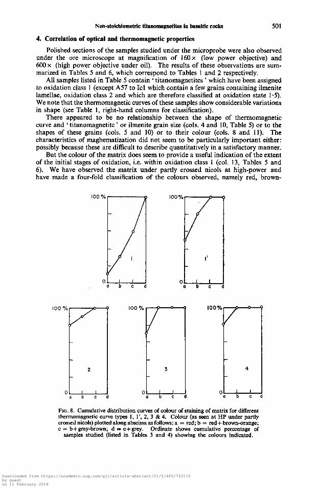
But the colour of the matrix does seem to provide a useful indication of the extent of the initial stages of oxidation, i.e. within oxidation class 1 (col. 13, Tables 5 and 6). We have observed the matrix under partly crossed nicols at high-power and have made a four-fold classification of the colours observed, namely red, brown-
)
100
O ’ O K , 0
a b c d
FIG. 8. Cumulative distribution curves of colour of staining of matrix for different thermomagnetic curve types 1, l‘, 2, 3 & 4. Colour (as seen at HP under partly crossed nicols) plotted along abscissa as follows: a = red; b = red + brown-mange; c = b+grey-brown; d = c+grey. Ordinate shows cumulative percentage of
samples studied (listed in Tables 3 and 4) showing the colours indicated.
Downloaded from https://academic.oup.com/gji/article-abstract/21/5/485/753110by gueston 11 February 2018

Tabl
e 5
Sam
ples
con
tain
ing
hom
ogen
eous
and
slig
htly
mag
hem
atiz
ed o
r gra
nula
ted
titan
omag
netit
es
(4)
Arg
entin
a 29
3 l(
e)
376
l(e)
T3
3 l’(
f)
117
3(a)
118
3(a)
13
9 2(
c)
152
2(d)
203
2(c)
T3
4 2(
g)
350-
2 10
-5
30-2
10
0-2
40
4
130-
1 30
00-2
50
-2
50-2
50
-2
100-
2 10
0-10
SE
sk
SE
SE
sk
SE
sk
SE
E
sk
E SE
sk
E
- PB
r G
Y
pP-B
r b
Gr-
Br
c
GY
b
PBr
Br-
Gy/
P a
P-Br
C
P-Br
P-
Br
- G
Y
P-Br
a
Gy-
Br
b
nil
4-l(2
0)
P-Br
30
4(15
) P-
Br
2&3(
10)
Gy-
Br
6-2(
10)
Gy-
Br
7-l(1
0)
P-Br
nil
0.5%
FeS
R
(sil)
fm
0.5%
FeS
fm 2
F
Br-
R s
il i &
fm
Or-
Br
st,
R s
il &
i pB
r st
(R s
t)
1% F
eS
(R-O
r st
) 1%
FeS
R
sil fm
P 1%
FeS
t 9
1%
TM
Cr c
ores
i P 0.
5% F
eS fm
2
8
A
A
(AX
W
A
6-2(
10)
P-Br
40
-1(1
5)
P-Br
Turk
ey
A57
2(
0)
A41
l’(
g)
D12
3 l(
n)
D12
7 l(
e)
G14
3 l(
i)
H12
2 l(
i)
T91
l(i)
K2
7 l(j
) A
106
3(d)
BT3
1 l’(
o)
100-
2 20
-10
4 100-
2 15
0-2
100-
2 45
0-2
250-
2 20
-2
100-
20
2 100-
4
SE
E sk
SE
E E E
E E SE
sk
SE
BD
F A
C
1.5
1 P-
Br
P-Br
b b
10-3
(5)
P-Br
PB
r
P-Br
PB
r pB
r pP
-Br
PBr
Cr-
Br
PBr
P-Br
R i
fm
Or
(Or s
il)
Or
sil
GY
(R fm
) GY
G
Y
GY
Gy
Or s
il (R
i)
Gy-
Or
st
C a 1%
FeS
FeS
0.5%
FeS
Downloaded from https://academic.oup.com/gji/article-abstract/21/5/485/753110by gueston 11 February 2018

Tabl
e 5
(con
tinue
d)
Gy
(R-B
r fm
) A
zore
s F
LlF
l l‘(
k)
300
E
(BH
F)
1 pP
-Br
a 20
(3)
P-B
r G
y 2
SE
FL7A
5 l’
(f)
250-
2 SE
A
1 P-
Br
a 12
-3(5
) P-
Br
Gy
Gy
Br s
t (R
sil)
FL
2Al
2(k)
50
-2
SE
AC
1
P-B
r b
20-2
(5)
pBr
GY
GY
(R f
m)
FL2A
2 2(
k)
50-2
SE
CD
1
P-B
r b
154(
10)
pBr
GY
G
Y (R
fm
)
FL2B
4 20
) 60
-2
SE
AC
1
pP-B
r/G
y a
10-2
(5)
pBr
GY
G
Y (R
i)
2 sk
D
2 sk
FL2D
2 4(
j) 30
0-2
SE
AB
CD
1
P-B
r a
40-1
(5)
pBr
GY
Br-
Or
st,
R
R s
il fm
& i
Ade
n H
21A
l’(
k)
150-
2 SE
AE
1’
P-Br
b
30-5
(5)
Gy-
Br
Gy
pBr
fm
Japa
n J9
3 l(
c)
200-
10
sk
BC
(F)
1 P-
Br
b 80
-5(5
) P-
Br
Gy
R-B
r fm
Ger
man
y R
K
l(1)
80
-2
EO
1
pP-B
r a
3-2(
8)
P-B
r G
y G
y fm
DE
G
5’
Paci
fic
TP3
8 2(
b)
1000
-2
SE
AE
(F)
1 P-
Br
b 60
0-25
(10)
P-
Br
Gy
GY
(R) f
m
Bul
garia
B1
l(
1)
100-
2 SE
0
1 G
y-B
r -
nil
GY
G
y-B
r B3
l(
1)
160-
2 SE 0
1 G
y-B
r -
nil
GY
(B
r fm
) B6
l(
m)
500-
2 SE
(C)
1 G
y-B
r -
nil
GY
(R f
m)
B9
l(m
) 20
0-2
SE 0
1 G
y-B
r a
25-l(
4)
GY
G
Y
B10
l(
m)
350-
2 SE 0
1 G
y-B
r a
25-l(
4)
GY
GY
Canary I
s. IC
3 l(
b)
100-
2 SE
0
1 C
r-Br
- ni
l G
Y
Gy-
Br
st
IC6
l’(a)
23
00-2
SE 0
1 C
r-Br
- ni
l GY
(R
) IC
16
l(a)
10
0-2
SE
AC
E
1 C
r-Br
- ni
l cy
pB
r st
ICl
4(g)
60
0-1
SE
AC
(F)
1.5
P-B
r b
3-l(1
0)
P-B
r G
y-B
r
0 a 0.
5% F
eS
1% F
eS
1% F
es. C
r cor
es in
TM
1%
FeS
1%
FeS
Cr cores i
n 1%
of
TM
Cr
cores in
50%
of T
M
Cr cores in
5%
of
TM
~
1
0
w
Downloaded from https://academic.oup.com/gji/article-abstract/21/5/485/753110by gueston 11 February 2018

Tabl
e 5
(con
rinue
d)
s P
Not
es
Col
. (1
): C
ount
ry of
orig
in.
Col
. (2
): Sa
mpl
e nu
mbe
r
Col
. (3
): Ty
pe o
f th
erm
omag
netic
cur
ve a
nd f
igur
e ke
y.
Col
. (4
): R
ange
of
grai
n sizes i
n m
icro
ns.
Col
. (5
): S
hape
of grains:-E
= eu
hedr
al; S
E =
sub-
euhe
dral
; sk
= sk
elet
al.
Col
. (6
): M
aghe
mat
izat
ion a
nd g
ranu
latio
n of
tita
nom
agne
tite g
rab
. A:
- co
ntai
ning
pat
ches
of
gre.
y/w
hite
mat
eria
l in
the
regi
on o
f cr
acks
/ble
mis
hes,
smal
l in
area
com
pare
d w
ith th
e gr
ain.
B:
- co
ntai
ning
pat
ches
of
grey
/whi
te m
ater
ial n
ot o
bvio
usly
ass
ocia
ted
with
cra
cks o
r oth
er fa
ults
. C:
- ba
nds
of g
rey/
whi
te a
long
edge
s and
/or
inte
rior t
o th
e gr
ain.
D
:- so
me
grai
ns h
ave
an o
vera
ll w
hitis
h/gr
ey c
olou
r cas
t. E:
- some gr
ains S
een
to c
onta
in ir
regu
lar v
einl
ets
of gr
ey/w
hite
mat
eria
l sur
roun
ding
isla
nds o
f ap
pare
ntly
una
ltere
d tit
anom
agne
tite.
F:-
occa
sion
al grain e
xhib
its il
men
ite la
mel
lae.
G
:- pr
esen
ce o
f tit
anom
agne
tite g
rain
s co
ntai
ning
gran
ules
of
rutil
e.
(XI.
(7):
Oxi
datio
n nu
mbe
r (d
eute
ric).
Col
. (8
): C
olou
r of
titan
omag
netit
es.
Col
. (9
): Pr
opor
tion
of i
lmen
ite in ore m
iner
als:-
(a
) les
s th
an 1
0 pe
r cen
t; (b
) bet
wee
n 10
and
50
per c
ent;
(c) m
ore
than
50
per
cent
.
Col
. (10
): Range
of g
rain
siz
es o
f ilm
enite
: ave
rage
leng
th-b
read
th r
atio
incl
uded
in
brac
kets
.
Col
. (11
): C
olou
r of
ilmen
ites.
Col
. (12
): G
ener
al c
olou
r of
pol
ished
sec
tion
view
ed a
t low
pow
er m
agni
ficat
ion
in u
npol
ariz
ed li
ght.
&I.
(13)
: G
ener
al c
olou
r and
des
crip
tion w
hen
view
ed u
nder
par
tly c
ross
ed n
icol
s at h
igh
pow
er m
agni
ficat
ion
( x 6
50).
Abb
revi
atio
ns ha
ve m
eani
ng a
s fol
low
s:-
frn =
ferr
omag
nesi
anq,
sil =
silic
ates
. i =
inte
rstit
ial,
st =
stai
ns.
Bra
cket
s in
dica
te th
at th
e fe
atur
es d
escr
ibed
do
not o
ccur
freq
uent
ly.
Col
. (14
): ad
ditio
nal n
otes
- Fe
S =
pyr
ites,
Cr =
chro
mile
, TM =
tita
nom
agne
tite.
ID L
4 P
Col
our a
bbre
viat
ions
(col
s 8.
11.
12 a
nd 1
3)
Gy,
gre
y; P
, pin
k; B
r, br
own;
Cr,
crea
m; R
, red
; Or,
oran
ge; p
, pal
e.
Downloaded from https://academic.oup.com/gji/article-abstract/21/5/485/753110by gueston 11 February 2018

Non-stoichiometric titanomagnetites in basaltic rocks 505
orange, grey-brown and grey. We have plotted in Fig. 8 curves showing the cumu- lative number of samples exhibiting a given type of thermomagnetic curve with the colour of the matrix observed as described above and note that these curves exhibit a notable correlation in the early stages of oxidation (within class 1) for samples which yield thermomagnetic curves of types 1, 1’ or 2. For more highly oxidized samples which yield thermomagnetic curves of types 3 or 4, no appreciable distinction can be drawn from observations of the colour of the matrix (including ferromag- nesians and feldspars) as it invariably exhibits patches of red rather than orange or brown.
5. Degree of oxidation of ‘ titanomagnetites ’ in basalts
Ideally this would be measured directly by the microprobe. But, in practice, difficulties arise in the accurate determination of oxygen when accompanied by titanium. This is because oxygen has a K absorption edge at 23.3 A while titanium has an L absorption edge in the same region. Thus when oxygen occurs in a sample containing titanium, the apparent concentration of oxygen depends on the amount of titanium present. The difference in oxygen content of ulvospinel and magnetite is small: the former contains 28.6 per cent by weight and the latter 27.6 per cent. However, the difference as ‘ seen ’ by the probe is enhanced by the titanium in ulvo- spinel. The nature of the corrections to be applied to a more complex natural sample become very important. They are large and at present are not known sufficiently well to permit the determination of oxygen with sufficient accuracy to determine the degree of non-stoichiometry. Hence, in the work described in this paper, we have adopted the method described below, involving a combination of microprobe and magnetic studies.
From the microprobe measurements we determine x, the molecular proportion of ulvospinel in the ‘ titanomagnetite ’ having made allowance for the ‘ impurity ’ cations contained as described in Section 2. We then note the difference between the measured and compositional Curie points, both of which are listed in Tables 1 and 2. This observed elevation of Curie temperature we attribute to oxidation to a cation deficient spinel. The commonly quoted data about the Curie points of these com- pounds are those published by Akimoto et al. (1957) but recently it has been shown that their samples were not single phase, i.e. they were not homogeneous cation deficient titanomagnetites as they originally supposed.
Recently, Readman & O’Reilly (1970, in preparation) have carried out new determinations of the Curie points of synthetic non-stoichiometric titanomagnetites by oxidizing wet-ground material in air at temperatures of 200-300”C. Their results are illustrated in Fig. 9. We used these contours to locate the points plotted in Fig. 10 where the compositions of our natural ‘ titanomagnetites ’ are represented.
On the triangular compositional diagrams of Figs 9 and 10, oxidation lines for constant Ti/Fe ratio run parallel to the base of the triangle; thus having obtained our x values from the microprobe analyses, we use the elevation of Curie temperature and the data of Fig. 9 to locate the compositions of the grains we studied and hence their degree of non-stoichiometry.
6. On the importance of cation deficient titanomagnetites in rock magnetism
Many investigations by numerous workers have been made into the question of whether a relationship exists between the polarity of remanent magnetization in rocks and their petrology, in particular to the state of oxidation of the ‘ titanomagnetites ’. While some workers claim to have found such a correlation (e.g. Wilson & Watkins 1967; Ade-Hall &Wilson 1969), others have failed to do so, e.g. Larson & Strangway (1966), Ade-Hall & Watkins (1970).
Downloaded from https://academic.oup.com/gji/article-abstract/21/5/485/753110by gueston 11 February 2018

Tabl
e 6
Sam
ples
con
tain
ing
titan
omag
netit
es w
ith il
men
ite la
mel
lae
Tita
nom
agne
tite g
rain
s Ilm
enite
gra
ins
Gen
eral
(1
) (2
) (3
) (4
) (5
) (6
) (8
) (9
) (1
0)
(11)
(1
2)
(13)
(1
4)
Arg
entin
a 11
5 4(
n)
60-2
SE
4.5
Gy-
Br
b 14
-3(8
) G
Y-l
k G
Y
Br-O
r-R
fm &
i 2"
ov
Turk
ey
Ore
gon
FlO
m
Ja
w
163
4(n)
12
0-10
28
9 4(
n)
60-2
31
7 4(
d)
50-2
4
B21
4(o)
50
-2
KY
9a2 401
) 20
0-1
319
4(s)
20
-1
326
4(s)
40-2
35
9 4(@
100-
2 36
6 4(
r)
50-2
37
7 4(
r)
60-2
20
-2
370
4(r)
20
-2
FLlA
6 2(
p)
50-2
FL
10C
44(h
) 20
0-2
J10
4(p)
30
-2
J20
4(p)
50
-2
J30
4(r)
60-2
J4
0 4(
r)
300-
2 J8
6 4(
r) 40
0-2
SE
5 SE
5 E
2.5
sk
E4
SE
3.
5
SE
4 SE
3.
5 SE
4.5
SE
3 E
2
sk
1
SE
5
E 3.
5 SE
3.
5
E 3.
5 E
2-5
E2
E
5.5
E3
Gy-
Br
Gy-
Br
pP-B
r P-
Br/G
y-B
r
P-Br
P-
Br
PBr
PBr
PBr
Cr-B
r C
r-Br
Cr-B
r PB
r
P-Br
P-
Br
P-Br
P-
Br
Cr-B
r P-
Br
Cr-B
r
b 18
0-5(
5)
PlB
r*
c 30
-2(1
0)
Gy-
Br*
b
14-2
(10)
P-
Br
b 15
-5(8
) P-
Br
a ve
rysm
all
P-B
r
a 10
-2(5
) G
y b
8-3(
10)
Cr-B
r b
9-3(
10)
Br*
b
u)-2
(4)
pBr*
b
40-5
(8)
b 50
-2(5
) G
y*
a 25
-2(5
) P-
Br*
a
25-2
(5)
P-B
r*
b 25
-5(8
) P-
Br*
a
15-5
(10)
pB
r*
a 15
-5(1
0)
pBr
b 40
-2(5
) pB
r-G
y ni
l G
y
Br-
Or-
R f
m, s
il &
i B
r-O
r R
fm, s
il &
i (R
i)
(2"
ov)
(2" ov)
0.5%
FeS
, (2"
ov)
F
g k cl
Br-
Or-
R
i 1
Br-
Or
sil
muc
h 2"
ov
I..
Or
st.
R i
& si
l R
i&fm
R
sil &
i O
r st
R i,
R s
il
P f B
r R
fm, s
il &
i
GY
R
fm, s
il &
i 2"
ov
GY
R
fm
muc
h 2"
ov
Br-
Gy
(R i
& si
l) G
Y
Rfm
&i
GY
GY
.
Ri&
fm
muc
h 2"
ov
(R i,
sil
& fr
n)
Or-B
r st
sil
Downloaded from https://academic.oup.com/gji/article-abstract/21/5/485/753110by gueston 11 February 2018

Tabl
e 6
(con
tinue
d)
Not
es
Col
. (1
): C
ount
ry of
orig
in.
Col
. (2
): S
ampl
e nu
mbe
r.
Col
. (3
): T
ype
of th
enno
mag
netic
curv
e an
d figure k
ey.
Col
. (4
): R
ange
of g
rain
sizes i
n microns.
Col
. (5
): S
hape
of grai
ns:-
E =
euhe
dral
; SE
= su
b-eu
hedr
al; s
k =
skel
etal
.
Col
. (6
): O
xida
tion
num
ber
(deu
teric
).
Col
. (8
): C
olou
r of t
itano
mag
netit
es.
Col
. (9
): P
ropo
rtio
n of
ilmen
ite in
ore m
iner
als;
(a) l
ess
than
10 per
cent
, (b)
bet
wee
n 10
and
50
per
cent
, (c)
mor
e th
an 5
0 pe
r cen
t.
Col
. (10
): R
ange
of
grai
n siz
es o
f ilm
enite
: ave
rage
leng
th-b
read
th r
atio
incl
uded
in b
rack
ets.
Col
. (11
): C
olou
r of
ilmen
ites:
*in
dica
tes p
rese
nce
of a
ssoc
iate
d ha
emat
ite.
Col
. (12
): G
ener
al c
olou
r of
polis
hed
sect
ion
view
ed a
t low
pow
er m
agni
ficat
ion
in u
npol
ariz
ed li
ght.
Col
. (13
): G
ener
al c
olou
r and
des
crip
tion
whe
n vi
ewed
und
er p
artly
cro
ssed
nic
ols
at h
igh
mag
nific
atio
n x
650)
.
Col
. (14
): 2
" ov
= se
cond
ary
ore
exso
lved
in p
yrox
enes
or o
livin
es.
Surr
ound
ing
brac
kets
indi
cate
infr
eque
nt o
ccur
renc
e.
Abb
revi
atio
ns a
s fol
low
s:-
fm =
ferr
omag
nesi
ans,
sil =
silic
ates
, i =
inte
rstit
ial;
infr
eque
nt f
eatu
res i
nclu
ded
in b
rack
ets.
B C
ols (
8),
(ll)
, (12
) and
(13)
: abb
revi
atio
ns fo
r col
ours
as
in T
able
3.
Downloaded from https://academic.oup.com/gji/article-abstract/21/5/485/753110by gueston 11 February 2018

508 K. M. Creer and J. D. Ibbetson
Ti 0,
1/3
' '2 Fe20s / I I
t I '
Fe 0 113 Feg, I /
FIG. 9. Curie (Nkl) temperature of cation deficient ' titanomagnetites ' (titano- maghematites). Curves obtained from experimental studies of wet-ground synthetic
material (after Readman).
One reason for this apparent lack of agreement may be that the critically important properties were not being observed. Thus, the state of deuteric oxidation has been described in terms of a five- or six-fold classification of increasing oxidation. We believe, however, that the more important magnetic transformations may occur within the oxidation class 1 and that they may be attributable to low temperature rather than deuteric oxidation. This is discussed at greater length by Creer & Petersen (1 969) and Creer er al. (1 969).
But we stress that on our model the (partial) self-reversal is produced by (magneto- static) interaction between a mother phase (the titanium-rich titanomagnetite initially present) and a daughter phase (an iron-rich titanomagnetite with Curie point above 50O0C, exsolved on a submicroscopic scale). Our model thus differs from those in which self-reversal occurs due to cation migration when titanomagnetites are oxidized to homogeneous cation deficient spinels. This latter process may also be important in nature, though we note that of the 20 points representing the integrated chemical composition of the oxidized titanomagnetites we have studied (Fig. lo), only one, viz. sample number 18 falls within the area of the ternary diagram where self-reversal of TRM occurs, i.e. where the net magnetization is due to the tetrahedral sites rather than to the oxtahedral sites as in an unoxidized or moderately oxidized titano- magnetite, assuming the O'Reilly-Banerjee (1967) model of cation distribution (Fig. 1 1 (a)). Thus the high states of oxidation required for self-reversal of TRM on this cation distribution model may have been achieved only rarely in nature.
Downloaded from https://academic.oup.com/gji/article-abstract/21/5/485/753110by gueston 11 February 2018

Non-stoichiometric titanomagnetites in basaltic rocks
TiOe
509
FIG. 10. Compositions of ' titanomagnetites ' contained in rocks studied in this paper determined from microprobe analysis and data from Fig. 8. Key to points asfol1ows:- 1 = sample293;2 = 376;3 = A41;4 = D123;5 = D127;6 = H122; 7 = T91; 8 = K27; 9 = RK; 10 = B1; 11 = B3; 12 = B6; 13 = B9; 14 = B10; 15 = Ic16:16 = Ic3;17 = T33;18 = BT31;19 = FL2a2(phasewithTc = 250°C);
19' = FL2a2 (phase with T, = 400 "C) and 20 = FL7a5.
( 0 ) (b)
FIO. 11. The range of compositions of oxidized titanomagnetites susceptible to self-reversal of NRM is indicated by the dotted shading. (a) For the O'Reilly- Banerjee (1967) model of cation distribution, and (b) for the Verboogen (1962) model. For the former model the compositional range in which the first-stage of oxidation only has occurred (i.e. in which only the Fez+ in B sites have been oxidized
to Fe3++) is shown by the diagonal shading.
Downloaded from https://academic.oup.com/gji/article-abstract/21/5/485/753110by gueston 11 February 2018

510 K. M. Creer and J. D. Ibbetson
On the Verhoogen (1962) model in which self-reversal is produced due to re- ordering of the cations as they migrate into their preferred sites from an initially random distribution, a rather wider range of compositions of cation deficient spinels is susceptible to self-reversal of remanence (Fig. ll(b)). In this model all the Fe3+ ions preferentially occupy A sites in the equilibrium distribution whereas in the O'Reilly-Banerjee model the lowest energy state is considered to be one in which B sites are occupied by a certain proportion of Fez+ as well as Fe3+.
We think that the Occurrence of partial and possibly of complete self-reversal due to progressive oxidation of titanomagnetite at normal temperatures over geo- logical time may be of importance in nature and in particular must be taken account of in the interpretation of marine magnetic anomalies (Creer, Petersen & Petherbridge 1970). But the mechanism may be one of sub-microscopic exsolution rather than of cation migration within a material which remains homogeneous.
Acknowledgments
The work was supported by a research grant for Rock and Mineral Magnetism from N.E.R.C. to which we express our thanks. We also take much pleasure in expressing our thanks and appreciation to Mr W. Davison who carefully and patiently carried out most of the microprobe measurements and who kept our Geoscan in working order.
Department of Geophysics and Planetary Physics,
University of Newcastle upon Tyne. School of Physics,
References
Ade-Hall, J. M., 1964. Electron probe microanalyser analyses of basaltic titano- magnetites and their significance to rock magnetism, Geophys. J. R . astr. SOC.,
Ade-Hall, J. M. & Wilson, R. L., 1963. Petrology and the natural remanence of the Mull lavas, Nature, 198, 659-660.
Ade-Hall, J. M. & Wilson, R. L., 1969. Opaque petrology and natural remanence polarity and natural remanence polarity in Mull (Scotland) dykes, Geophys. J. R. astr. Sac., 18, 333.
Ade-Hall, J. M., Wilson, R. L. & Smith, P. J., 1965. The petrology, Curie points and natural magnetisations of basic lavas, Geophys. J. R. astr. SOC., 9, 323-336.
Ade-Hall, J. M. & Watkins, N. D., 1970. Absence of correlations between opaque petrology and natural remanence polarity in Canary Island lavas, Geophys. J. R. astr. SOC., 19, 351-360.
Akimoto, S., Katsura, T. k Yoshida, M., 1957. Magnetic properties of TiFe,O,-Fe,O, system and their change with oxidation, J. Geomagn. Geoelect. Kyoto, 9, 165.
Carmichael, I. S. E. & Nicholls, J., 1967. Iron-titanium oxides and oxygen fugacities in volcanic rocks, J. geophys. Res., 72, 4665-4687.
Creer, K. M., Ibbetson, J. & Drew, W., 1969. Activation energy of cation migration in titanomagnetites, Geophys. J. R. astr. SOC., 19, 93-101.
Creer, K. M. & Petersen, N., 1969. Thermochemical magnetisation in basalts, Z. Geophys., 501-516.
Creer, K. M., Petersen, N. & Petherbridge, W., 1970. Partial self-reversal of remanent magnetization and viscous magnetization in basalts, Geophys. J. R. astr. SOC., 21, 471-483.
Frohlich, F., Loffler, H. & Stiller, H., 1965. Interpretations of changes in Curie temperatures observed in rocks, Geophys. J. R. astr. SOC., 9, 411-412.
8, 301-312.
Downloaded from https://academic.oup.com/gji/article-abstract/21/5/485/753110by gueston 11 February 2018

Non-stoichiometric titanomagnetites in basaltic rocks 51 1
Heinrich, K. F. J., 1968a. Common sources of error in electron probe microanalysis.
Heinrich, K. F. J., 1968b. Electron probe microanalysis: A Review, Appl. Spectrosc.,
Larson, S . E. & Strangway, D. W., 1966. Magnetic polarity and igneous petrology,
Long, J. V. P. & Sweatman, T. R., 1969. Quantitative electron-probe microanalysis
Nagata, T., 1961. Rock Magnetism, p. 87, Maruzen Co. Ltd. O’Reilly, W. & Banerjee, S. K., 1967. The mechanism of oxidation in titano-
magnetites: a magnetic study, Min. Mag., 36, 29-37. Ozima, M. & Larson, E. E., 1969. Low and high temperature oxidation of titano-
magnetite in relation to irreversible changes in the magnetic properties of sub- marine basalts (abstract only), Trans. Am. geophys. Union, 50, 132.
A method for calculating the absorption correction in electron- probe microanalysis, X-ray optics and X-ray microanalysis, Eds Pattee, H. H. & Cosslett, V. F., Arne Engstrom. A.P., 379-392.
Pouillard, E., 1950. Sur le Comportement de 1’Alumine et de 1’Oxyde de Titane vis-a-vis des Oxydes de Fer, Ann. chinz., 12, 164214.
Reed, S. J. B., 1965. Characteristic fluorescence corrections in electron-probe microanalysis, Brit. J. appl. Phys., 16, 913426.
Sanver, M. & O’Reilly, W., 1970. Identification of naturally occurring non- stoichiometric titanomagnetites, P.E.P.Z., 2, 166-1 74.
Schult, A., 1968. Self-reversal of magnetization and chemical composition of titanomagnetites in basalts, Earth Planet. Sci. Lett., 4, 57-63.
Smith, J. V., 1965. X-ray-emission microanalysis of rock-forming minerals, J. Geol., 73, 830-864.
Smith, P. J., 1967. Electron probe microanalysis of optically homogeneous titano- magnetites and ferrian ilmenites in basalts of palaeomagnetic significance, J. geophys. Res., 72, 5087-5100.
Smith, P. J., 1968. Palaeomagnetism and the compositions of highly-oxidised iron- titanium oxides in basalts, Phys. earth. planet. Znt., 1, 88-92.
Verhoogen, J., 1962. Oxidation of iron-titanium oxides in igneous rocks, J. geol.,
Verhoogen, J., 1956. Ionic ordering and self-reversal of magnetisation in impure magnetites, J. geophys. Res., 61, 201.
Vincent, E. N., 1960. N . Jb. Miner. Abh., 96, 993-1016.
Wright, J. B., 1964. Iron-titanium oxides in some New Zealand iron sands, N. Zealand J. Geol. Geophys., 7, 424-444.
Wright, J. B. & Lovering, J. F., 1965. Electron-probe microanalysis of the optically homogeneous titanomagnetites and ferrian ilmenites in basalts of palaeomagnetic significance, Min. Mag., 35, 604621.
Wright, J. B., 1967. Self-reversal and field reversal in palaeomagnetism, Geophys. J. R . astr. SOC., 12, 511-516.
Wilson, R. L., 1966. Further correlations between the petrology and natural magnetic polarity of basalts, Geophys. J. R. astr. Soc., 10, 413420.
Wilson, R. L. & Watkins, N. D., 1967. Correlation of petrology and natural magnetic polarity in ColumbiaPlateau basalts, Geophys. J. R. astr. Soc., 12,405425.
Wilson, R. L., Haggerty, S. F. & Watkins, N. D., 1968. Variation of palaeomagnetic stability and other parameters in a vertical traverse of a single Icelandic lava, Geophys. J. R. astr. Soc., 16, 79-96.
Yakowitz, H. & Heinrich, K. F. J., 1968. Quantitative electron probe microanalysis: absorption correction uncertainty I, Microchim. Acta., 182-200.
Advances in X-ray analysis Vol. ZZ, 40-55. Plenum Press, New York.
22, Part I, 395-403.
Nature, 212, 756-757.
of rock-forming minerals, J. Petrology, 10, Part 2, 332-379.
Philibert, J., 1963.
70, 168-181.
Ulvospinel in the Skaergaard Intrusion, Greenland,
Downloaded from https://academic.oup.com/gji/article-abstract/21/5/485/753110by gueston 11 February 2018