Electromigration Reliability Analysis of Power Delivery ... · Electromigration Reliability...
89
Electromigration Reliability Analysis of Power Delivery Networks in Integrated Circuits by Mohammad Fawaz A thesis submitted in conformity with the requirements for the degree of Master of Applied Sciences Graduate Department of Electrical & Computer Engineering University of Toronto c Copyright 2013 by Mohammad Fawaz
Transcript of Electromigration Reliability Analysis of Power Delivery ... · Electromigration Reliability...

Electromigration Reliability Analysis of Power Delivery
Networks in Integrated Circuits
by
Mohammad Fawaz
A thesis submitted in conformity with the requirementsfor the degree of Master of Applied Sciences
Graduate Department of Electrical & Computer EngineeringUniversity of Toronto
c© Copyright 2013 by Mohammad Fawaz
Abstract
Electromigration Reliability Analysis of Power Delivery Networks in Integrated Circuits
Mohammad Fawaz
Master of Applied Sciences
Graduate Department of Electrical & Computer Engineering
University of Toronto
2013
Electromigration in metal lines has re-emerged as a significant concern in modern VLSI
circuits. The higher levels of temperature and the large number of EM checking strate-
gies, have led to a situation where trying to guarantee EM reliability often leads to
conservative designs that may not meet the area or performance specs. Due to their
mostly-unidirectional currents, the problem is most significant in power grids. Thus, this
work is aimed at reducing the pessimism in EM prediction. There are two sources for
the pessimism: the use of the series model for EM checking, and the pessimistic assump-
tions about chip workload. Therefore, we propose an EM checking framework that allows
users to specify conditions-of-use type constraints to capture realistic chip workload, and
which includes the use of a novel mesh model for EM prediction in the grid, instead of
the traditional series model.
ii

Acknowledgements
It would not have been possible to write this thesis without the immense help and support
of the amazing people around me. I owe a very important debt to all of those who were
there when I needed them most.
First and above all, I would like to thank my supervisor Professor Farid N. Najm, who
supported me throughout my thesis with his great patience, regular encouragement, and
continuous advice. Professor Najm is easily the best advisor anyone could ever hope for;
his deep insight, professional leadership, and warm friendliness were key factors without
which the development of this work would not have been possible. Thank you professor
for your overwhelming efforts and for your mentorship on both professional and personal
levels.
I am also thankful for Professors Jason Anderson, Andreas Veneris, and Costas Sarris,
from the ECE department at the University of Toronto, for reviewing this work and
providing their valuable comments.
I would also like to thank Abhishek for his guidance and support throughout the first
half of my degree program. Abhishek was always there to answer my questions and to
discuss new research ideas. Special thanks go to my colleague and my friend Sandeep
Chatterjee who’s work was closely related to mine. A major part of this research was done
in collaboration with him, especially the content of Chapter 3. The many long discussions
we had helped a lot in understanding the problem and in shaping the proposed solutions.
Zahi “zehe” Moudallal, my colleague and one of my best friends, deserves a very
special mention. I thank him for all the great times we had inside and outside the lab.
The long working hours would not have been the same without his presence and his sense
of humor. I wish him best of luck in all his future endeavors.
I am also grateful to Noha “noni” Sinno for her friendship and her constant support
over the past two years. Thank you Noha for the fun times and for all the long discussions
we had about life in general; they helped me face the world with a better attitude. I
must also express my gratitude to Elias “ferzol” El-ferezli who helped me a lot when I
first arrived to Toronto. His friendship, advice, and assistance were key in surviving the
first few months away from home and in making me a better person overall.
Of my friends at the University of Toronto, I would like to thank Dr. Hayssam
Dahrouj for his motivation, Agop Koulakezian for all the help, as well as my office mates
in Pratt building, room 392, for making the lab a great and pleasant environment. I wish
them the best and the brightest futures.
Last but not least, I would like thank my parents Bassam Fawaz and Jamila Fawaz,
to whom I dedicate this work, for always encouraging me and investing their time and
iii

money in my future. Thank you for your constant support and advice, and for always
believing in me and making me who I am today. I would also like to thank my two
younger brothers Hassan and Hussein and wish them the best of luck in achieving their
future goals.
iv

Contents
1 Introduction 1
1.1 Motivation . . . . . . . . . . . . . . . . . . . . . . . . . . . . . . . . . . . 1
1.2 Contributions . . . . . . . . . . . . . . . . . . . . . . . . . . . . . . . . . 2
1.3 Organization . . . . . . . . . . . . . . . . . . . . . . . . . . . . . . . . . 3
2 Background 4
2.1 Introduction . . . . . . . . . . . . . . . . . . . . . . . . . . . . . . . . . . 4
2.2 Electromigration . . . . . . . . . . . . . . . . . . . . . . . . . . . . . . . 4
2.2.1 Flux Divergence . . . . . . . . . . . . . . . . . . . . . . . . . . . . 5
2.2.2 Blech Effect . . . . . . . . . . . . . . . . . . . . . . . . . . . . . . 5
2.2.3 Failure Models . . . . . . . . . . . . . . . . . . . . . . . . . . . . 6
2.3 Reliability Mathematics . . . . . . . . . . . . . . . . . . . . . . . . . . . 7
2.3.1 Overview . . . . . . . . . . . . . . . . . . . . . . . . . . . . . . . 7
2.3.2 Reliability Measures . . . . . . . . . . . . . . . . . . . . . . . . . 7
2.3.3 Time-to-Failure Distributions . . . . . . . . . . . . . . . . . . . . 10
2.4 Traditional Electromigration Checking . . . . . . . . . . . . . . . . . . . 13
2.4.1 Current Density Limits . . . . . . . . . . . . . . . . . . . . . . . . 13
2.4.2 Statistical Electromigration Budgeting (SEB) . . . . . . . . . . . 13
2.5 Electromigration in the Power Grid . . . . . . . . . . . . . . . . . . . . . 14
2.5.1 Overview . . . . . . . . . . . . . . . . . . . . . . . . . . . . . . . 14
2.5.2 Power Grid Model . . . . . . . . . . . . . . . . . . . . . . . . . . 16
2.6 Sampling and Statistical Estimation . . . . . . . . . . . . . . . . . . . . . 20
2.6.1 Overview . . . . . . . . . . . . . . . . . . . . . . . . . . . . . . . 20
2.6.2 Sampling from the Standard Normal . . . . . . . . . . . . . . . . 20
2.6.3 Sampling from the Lognormal . . . . . . . . . . . . . . . . . . . . 21
2.6.4 Mean Estimation by Random Sampling . . . . . . . . . . . . . . . 21
2.6.5 Probability Estimation by Random Sampling . . . . . . . . . . . 24
2.7 Notation . . . . . . . . . . . . . . . . . . . . . . . . . . . . . . . . . . . . 25
v

3 Vector-Based Power Grid Electromigration Checking 26
3.1 Introduction . . . . . . . . . . . . . . . . . . . . . . . . . . . . . . . . . . 26
3.2 The ‘Mesh’ Model . . . . . . . . . . . . . . . . . . . . . . . . . . . . . . . 27
3.3 Estimation Approach . . . . . . . . . . . . . . . . . . . . . . . . . . . . . 28
3.3.1 MTF and Survival Probability Estimation . . . . . . . . . . . . . 28
3.3.2 Resistance Evolution . . . . . . . . . . . . . . . . . . . . . . . . . 28
3.3.3 Generating Time-to-Failure Samples . . . . . . . . . . . . . . . . 29
3.4 Computing Voltage Drops . . . . . . . . . . . . . . . . . . . . . . . . . . 30
3.4.1 Sherman-Morrison-Woodbury Formula . . . . . . . . . . . . . . . 32
3.4.2 The Banachiewicz-Schur Form . . . . . . . . . . . . . . . . . . . . 33
3.4.3 Case of Singularity . . . . . . . . . . . . . . . . . . . . . . . . . . 36
3.5 Implementation . . . . . . . . . . . . . . . . . . . . . . . . . . . . . . . . 37
3.6 Experimental Results . . . . . . . . . . . . . . . . . . . . . . . . . . . . . 39
3.7 Conclusion . . . . . . . . . . . . . . . . . . . . . . . . . . . . . . . . . . . 41
4 Vectorless Power Grid Electromigration Checking 43
4.1 Introduction . . . . . . . . . . . . . . . . . . . . . . . . . . . . . . . . . . 43
4.2 Problem Definition . . . . . . . . . . . . . . . . . . . . . . . . . . . . . . 43
4.2.1 Modal Probabilities . . . . . . . . . . . . . . . . . . . . . . . . . . 44
4.2.2 Current Feasible Space . . . . . . . . . . . . . . . . . . . . . . . . 46
4.3 Optimization . . . . . . . . . . . . . . . . . . . . . . . . . . . . . . . . . 48
4.3.1 Local Optimization . . . . . . . . . . . . . . . . . . . . . . . . . . 49
4.3.2 Exact Global Optimization . . . . . . . . . . . . . . . . . . . . . . 55
4.4 Experimental Results . . . . . . . . . . . . . . . . . . . . . . . . . . . . . 57
4.5 Conclusion . . . . . . . . . . . . . . . . . . . . . . . . . . . . . . . . . . . 59
5 Simulated Annealing Based Electromigration Checking 60
5.1 Introduction . . . . . . . . . . . . . . . . . . . . . . . . . . . . . . . . . . 60
5.2 Simulated Annealing for Continuous Problems . . . . . . . . . . . . . . . 60
5.2.1 Overview . . . . . . . . . . . . . . . . . . . . . . . . . . . . . . . 60
5.2.2 Main Algorithm . . . . . . . . . . . . . . . . . . . . . . . . . . . . 61
5.2.3 The Acceptance Function . . . . . . . . . . . . . . . . . . . . . . 62
5.2.4 Cooling Schedule . . . . . . . . . . . . . . . . . . . . . . . . . . . 62
5.2.5 Next Candidate Distribution . . . . . . . . . . . . . . . . . . . . . 63
5.2.6 Stopping Criterion . . . . . . . . . . . . . . . . . . . . . . . . . . 66
5.3 Simulated Annealing with Local Optimization . . . . . . . . . . . . . . . 67
5.4 Optimization with Changing Currents . . . . . . . . . . . . . . . . . . . 67
vi

5.4.1 Estimating EM Statistics for Step Currents . . . . . . . . . . . . 67
5.4.2 Optimization . . . . . . . . . . . . . . . . . . . . . . . . . . . . . 69
5.5 Optimization with Selective Updates . . . . . . . . . . . . . . . . . . . . 70
5.6 Experimental Results . . . . . . . . . . . . . . . . . . . . . . . . . . . . . 71
5.7 Conclusion . . . . . . . . . . . . . . . . . . . . . . . . . . . . . . . . . . . 74
6 Conclusion and Future Work 76
Bibliography 78
vii

List of Tables
3.1 Comparison of power grid MTF estimated using the series model and the
mesh model . . . . . . . . . . . . . . . . . . . . . . . . . . . . . . . . . . 40
3.2 Survival probability estimation . . . . . . . . . . . . . . . . . . . . . . . 40
4.1 Exact average minimum TTF computation . . . . . . . . . . . . . . . . . 58
5.1 Speed and accuracy comparison between the first Simulated Annealing
based method and the exact solution of chapter 4 . . . . . . . . . . . . . 70
5.2 Comparison of power grid average minimum TTF and CPU time for the
three Simulated Annealing based methods . . . . . . . . . . . . . . . . . 71
viii
List of Figures
2.1 A triple point in a wire . . . . . . . . . . . . . . . . . . . . . . . . . . . . 5
2.2 Standard normal and lognormal distributions . . . . . . . . . . . . . . . . 12
2.3 High level model of the power grid . . . . . . . . . . . . . . . . . . . . . 16
2.4 A resistive model of a power grid . . . . . . . . . . . . . . . . . . . . . . 17
2.5 A small resistive grid . . . . . . . . . . . . . . . . . . . . . . . . . . . . . 19
3.1 Resistance evolution . . . . . . . . . . . . . . . . . . . . . . . . . . . . . 29
3.2 Mesh model MTF estimation . . . . . . . . . . . . . . . . . . . . . . . . 38
3.3 CPU time of MTF estimation using the mesh model . . . . . . . . . . . . 41
3.4 Estimated statistics for grid DC3 (200K nodes) . . . . . . . . . . . . . . 42
4.1 Choosing the next starting point I(2) . . . . . . . . . . . . . . . . . . . . 55
4.2 CPU time of the exact approach versus the number of grid nodes . . . . 59
5.1 Generating lambda . . . . . . . . . . . . . . . . . . . . . . . . . . . . . . 65
5.2 One way of reflecting yk+1 back into X to obtain yk+1 = yk+1 . . . . . . . 66
5.3 CPU time of the Simulated Annealing based methods versus the number
of grid nodes . . . . . . . . . . . . . . . . . . . . . . . . . . . . . . . . . 73
5.4 Average minimum TTF estimated for the three Simulated Annealing based
methods versus the number of grid nodes . . . . . . . . . . . . . . . . . . 74
5.5 Simulated Annealing progress for a particular TTF sample using all the
three proposed methods (33K grid) . . . . . . . . . . . . . . . . . . . . . 75
ix

Chapter 1
Introduction
1.1 Motivation
The on-die power grid in integrated circuits (IC) is the electric network that provides
power from the power supply pins on the package to the on-die transistors. The power
grid must supply a source of power that is fairly free from fluctuations over time. A large
drop in supply voltage may lead to timing violations or logic failure. With technology
scaling, power grid verification, which involves checking that the voltage levels provided
to the underlying logic are within an acceptable range, has become a critical step in any
IC design. Unfortunately, it is not enough to check the performance of the grid at the
fabrication time; a well designed power grid must continue to deliver the required voltage
levels to all circuit nodes for a certain number of years before failing.
Electromigration (EM), a long term failure mechanism that affects metal lines, is a
key problem in VLSI especially in the power grid. The gradual transport of metal atoms
caused by electromigration leads to the creation of a void which significantly increases
the resistance of the line in consideration and can lead to an open circuit. This affects the
power distribution to the underlying logic and may cause harmful voltage fluctuations.
Checking for electromigration in a power grid involves computing its mean time-to-failure,
which gives the designer an idea about the robustness of the grid and whether it needs
to be redesigned or not.
What is most worrying is that existing electromigration checking tools provide pes-
simistic results, and hence the safety margins between the predicted EM stress and the
EM design rules are becoming smaller. Historically, electromigration checking tools relied
on worst-case current density limits for individual grid lines. Later on, Statistical Electro-
migration Budgeting (SEB) was introduced in [1] in which the series model is employed
with other simplifying assumptions leading to a simple expression of the failure rate as
1

Chapter 1. Introduction 2
the sum of failure rates of individual components, and became a standard technique in
many industrial CAD tools. SEB is appealing because it relates the reliability of circuit
components to the reliability of the whole system. In addition, SEB is simple to use and
allows some components to have high failure rates as long as the sum of all the failure
rates is acceptable.
Nonetheless, modern power grids are meshes rather than the traditional “comb” struc-
ture. The mesh structure allows multiple paths between any two nodes, and accordingly,
modern grids have some level of redundancy that must be considered to get a better
prediction of the lifetime of the grid. Moreover, the rate of EM degradation in power
grid lines depends on the current density, and hence on the patterns of current drawn by
the underlying circuitry. It is impractical to assume that the exact current waveforms are
available for all the chip workload scenarios. Also, one might need to verify the grid early
in the design flow where a limited amount of workload information is available. There-
fore, a vectorless approach is needed to deal with the uncertainties about the underlying
logic behavior. A vectorless technique is a technique that does not require the exact
current waveforms nor specific chip input vectors; it can verify the chip using limited
information about the circuit operation.
1.2 Contributions
The goal of this research is to develop an efficient, less pessimistic, and vectorless
electromigration checking tool for mesh power grids. We first propose a vector-based tech-
nique which computes the mean time-to-failure of the power grid using a more accurate
model than SEB and which assumes that the current waveforms are available exactly. A
vector-based technique is a technique that requires the exact currents drawn by the chip
based on a specific chip input vector. This step is necessary to explain our model and
will be a basis for our other contributions. The engine developed can also be used to
compute the survival probability of the grid for a certain number of years as well as to
derive its reliability function.
To overcome user uncertainty about the chip workload, we also propose a vector-
less framework which extends the vector-based engine to the case where partial current
specifications are available in the form of constraints on the currents and on the usage
frequencies of different power modes. In this domain, our first contribution is an exact
but expensive approach which relies on solving a set of linear and mixed integer opti-
mization problems. The exact approach is interesting and only useful when the grid is
small or when only certain parts of the grid need to be verified.

Chapter 1. Introduction 3
To deal with larger grids, we propose three other approximate approaches that are
based on the use of Simulated Annealing [2]. The proposed approaches provide fairly
accurate results as well as significant speed up over the exact solution.
1.3 Organization
This thesis is organized as follows: Chapter 2 develops all the necessary background ma-
terial on electromigration, reliability mathematics, and the power grid model. Chapter 3
describes the new vector-based checking model which takes the redundancy of the grid
into account. Chapter 4 presents our exact approach for vectorless power grid EM check-
ing, and Chapter 5 shows Simulated Annealing-based approaches. We conclude with
future research directions in Chapter 6.

Chapter 2
Background
2.1 Introduction
In this chapter, we present a review of all the background material needed for this work.
Section 2.2 discusses the the physics of electromigration as well as the basic mathematical
models associated with it. In Section 2.3, we cover the mathematical functions describing
the reliability of a physical system. In Section 2.4 we present the existing electromigra-
tion checking techniques including current density limits checks and most importantly
Statistical Electromigration Budgeting. In Section 2.5 we turn our focus on the power
grid and its model. We also discuss the reasons why checking for electromigration in the
power grid is critical for the safety of the chip. Section 2.6 presents a summary of the
basic sampling techniques as well some of the existing mean and probability estimation
methods. The last Section introduces few notations that will be useful throughout the
thesis.
2.2 Electromigration
Electromigration in metal lines is the gradual transport of metal caused by the momentum
exchange between the conducting electrons and the diffusing metal atoms. Over time,
metal diffusion causes a depletion of enough material so as to create an open circuit. A
pile-up of metal (called hillock) can also occur and can cause a short circuit between
neighboring wires, but this phenomena is usually suppressed and ignored in modern IC
due to the layers of other material around the wires. In this work, we will only consider
the effect of voids on the lifetime of the power grid while ignoring the effect of shorts
that could occur between neighboring lines due to hillocks.
4
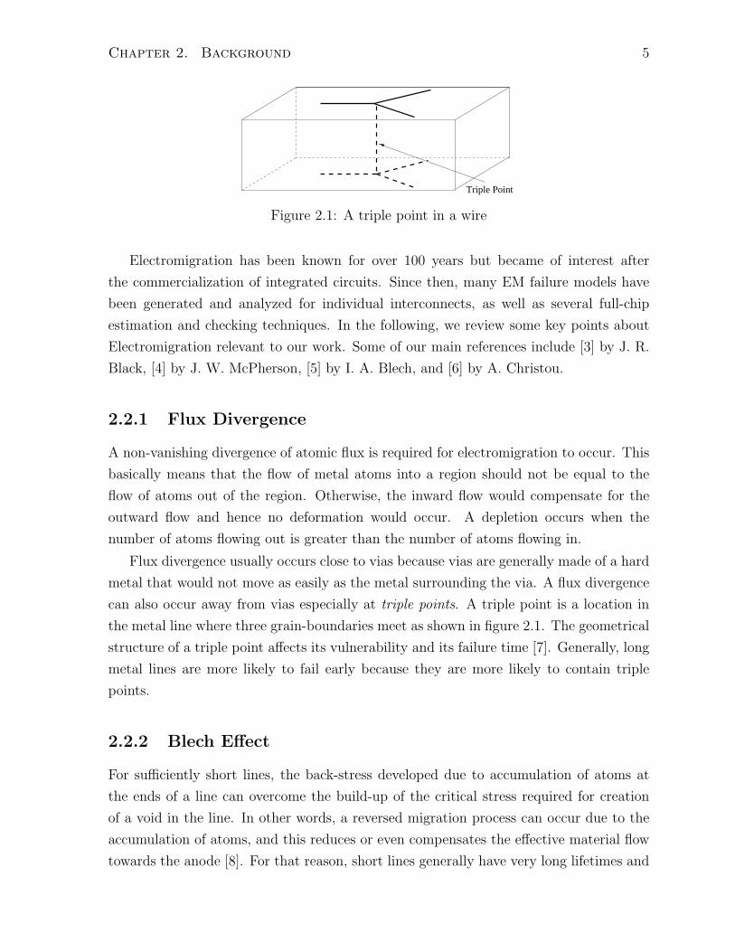
Chapter 2. Background 5
Triple Point
Figure 2.1: A triple point in a wire
Electromigration has been known for over 100 years but became of interest after
the commercialization of integrated circuits. Since then, many EM failure models have
been generated and analyzed for individual interconnects, as well as several full-chip
estimation and checking techniques. In the following, we review some key points about
Electromigration relevant to our work. Some of our main references include [3] by J. R.
Black, [4] by J. W. McPherson, [5] by I. A. Blech, and [6] by A. Christou.
2.2.1 Flux Divergence
A non-vanishing divergence of atomic flux is required for electromigration to occur. This
basically means that the flow of metal atoms into a region should not be equal to the
flow of atoms out of the region. Otherwise, the inward flow would compensate for the
outward flow and hence no deformation would occur. A depletion occurs when the
number of atoms flowing out is greater than the number of atoms flowing in.
Flux divergence usually occurs close to vias because vias are generally made of a hard
metal that would not move as easily as the metal surrounding the via. A flux divergence
can also occur away from vias especially at triple points. A triple point is a location in
the metal line where three grain-boundaries meet as shown in figure 2.1. The geometrical
structure of a triple point affects its vulnerability and its failure time [7]. Generally, long
metal lines are more likely to fail early because they are more likely to contain triple
points.
2.2.2 Blech Effect
For sufficiently short lines, the back-stress developed due to accumulation of atoms at
the ends of a line can overcome the build-up of the critical stress required for creation
of a void in the line. In other words, a reversed migration process can occur due to the
accumulation of atoms, and this reduces or even compensates the effective material flow
towards the anode [8]. For that reason, short lines generally have very long lifetimes and

Chapter 2. Background 6
in many cases, can be considered immortal; this is called the Blech Effect [5].
The Blech effect is quantified is terms of a critical value of the product of current
density (J) and length of a line (L), denoted βc. For modern IC, βc ranges between
2000A/cm and 10, 000A/cm.
This threshold value is very useful in circuit design. It determines whether a line is
immortal or not as follows: given a line ℓ of length Lℓ, subject to a current density Jℓ,
then ℓ is considered EM -immune (i.e. immortal) if JℓLℓ < βc and EM -susceptible if
JℓLℓ ≥ βc.
2.2.3 Failure Models
Since the degradation rate depends on the microstructure of a line which varies from
chip to chip, electromigration is considered to be a statistical phenomena. This means
that the time-to-failure of a mortal line under the effect of electromigration is a random
variable. It has been established for a while that EM failure times have a good fit to
a lognormal (LN) distribution, i.e. its logarithm has a normal (Gaussian) distribution.
Other, possibly more accurate models have been proposed such as the multilognormal
distribution [9] and the shifted lognormal distribution [7], however, the lognormal remains
the simplest and the most practical distribution to use.
The most commonly used expression for the mean time-to-failure (MTF) of a mortal
line is Black’s equation [6]:
MTF =a
AJ−η exp
(
Ea
kT
)
(2.1)
where A is an experimental constant that depends on the physical properties of the metal
line (volume resistivity, etc.), a is the cross sectional area of the line, J is the effective
current density, η is the current exponent that depends on the material of the wire and
the failure stage (η > 0), k is the Boltzmann’s constant, T is the temperature in Kelvin,
and Ea is the activation energy for EM.
Most of the references report a value between 1 and 2 for η. A value close 1 usually
indicates that the lifetime is dominated by the time taken by the void to grow, while
a value close 2 indicates that void nucleation (the accumulation of vacancies at sites of
flux divergence) is the dominant phase of the lifetime. Other references such as [4] report
different values for different metal systems: typical values are ≈ 2 for aluminum alloys
and ≈ 1 for copper.

Chapter 2. Background 7
2.3 Reliability Mathematics
2.3.1 Overview
In this section, we cover the reliability measures of a physical system based on a system
theoretic approach. This means that only the input-output properties of the system are
of interest, and not how it is built internally [10]. We start by a definition of reliability
and then we introduce the mathematical functions that describe it.
Definition 1. Reliability is the probability of performing a certain function without
failure for specific period of time.
This definition has the following four main elements:
1. Probability: The exact time-to-failure of a system is usually unpredictable be-
cause it depends on several stochastic physical phenomena. Accordingly, reliability
is a probability, i.e. a number between zero and one.
2. Function: The system under consideration must be evaluated based on a specific
functionality.
3. Failure: What constitutes a failure in a physical system must be well defined before
one can estimate its reliability. A system is said to fail when it becomes unable to
perform as intended.
4. Time: The system must perform for a period of time and hence reliability almost
always depends on time.
There are many mathematical metrics that describe the reliability of a system. In the
following we present the ones relevant to our work.
2.3.2 Reliability Measures
Let T be the time-to-failure of a system. We assume that T is the time to first failure
and that the system remains failed for all future time (i.e. the system is non-repairable).
Also, we assume that the system is working properly at time t = 0. This allows defin-
ing T as a continuous random variable (RV) with the following cumulative distribution
function (CDF):
F (t) = Pr{T ≤ t}, t > 0 (2.2)
Chapter 2. Background 8
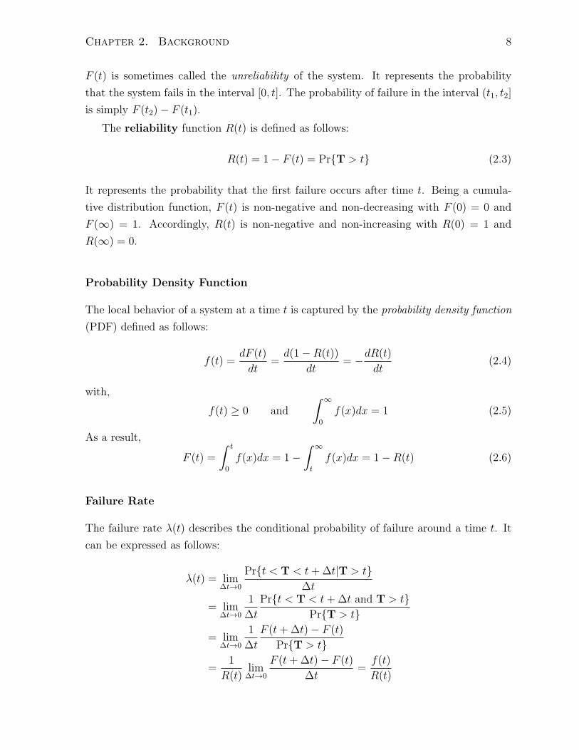
F (t) is sometimes called the unreliability of the system. It represents the probability
that the system fails in the interval [0, t]. The probability of failure in the interval (t1, t2]
is simply F (t2)− F (t1).The reliability function R(t) is defined as follows:
R(t) = 1− F (t) = Pr{T > t} (2.3)
It represents the probability that the first failure occurs after time t. Being a cumula-
tive distribution function, F (t) is non-negative and non-decreasing with F (0) = 0 and
F (∞) = 1. Accordingly, R(t) is non-negative and non-increasing with R(0) = 1 and
R(∞) = 0.
Probability Density Function
The local behavior of a system at a time t is captured by the probability density function
(PDF) defined as follows:
f(t) =dF (t)
dt=d(1−R(t))
dt= −dR(t)
dt(2.4)
with,
f(t) ≥ 0 and
∫ ∞
0
f(x)dx = 1 (2.5)
As a result,
F (t) =
∫ t
0
f(x)dx = 1−∫ ∞
t
f(x)dx = 1−R(t) (2.6)
Failure Rate
The failure rate λ(t) describes the conditional probability of failure around a time t. It
can be expressed as follows:
λ(t) = lim∆t→0
Pr{t < T < t+∆t|T > t}∆t
= lim∆t→0
1
∆t
Pr{t < T < t+∆t and T > t}Pr{T > t}
= lim∆t→0
1
∆t
F (t+∆t)− F (t)Pr{T > t}
=1
R(t)lim∆t→0
F (t+∆t)− F (t)∆t
=f(t)
R(t)

Chapter 2. Background 9
Basically, for small ∆t, the product λ(t)∆t represents the probability of failure in the
interval [t, t+∆t] under the condition that the system has survived until time t.
It is sometimes useful to express R(t) as a function of λ(t). To do that, we use (2.4)
to write:
λ(t) =f(t)
R(t)= − 1
R(t)
dR(t)
dt= − d
dt(lnR(t)) (2.7)
Integrating both sides between 0 to t:
∫ t
0
λ(x)dx = − (lnR(t)− lnR(0)) (2.8)
Because R(0) = 1, we obtain:
R(t) = exp
(
−∫ t
0
λ(x)dx
)
(2.9)
The Mean time-to-failure (MTF)
The mean time-to-failure is the expected value of the random variable T:
MTF = E[T] =
∫ ∞
0
tf(t)dt (2.10)
Knowing the fact that f(t) = −dR(t)dt
, we can write:
MTF = −∫ ∞
0
tdR(t) (2.11)
Integrating by parts:
MTF = −[
tR(t)
∣
∣
∣
∣
∞
0
−∫ ∞
0
R(t)dt
]
(2.12)
Clearly, tR(t)
∣
∣
∣
∣
0
= 0. Also, for most statistical distributions encountered in the study of
circuit reliability, R(t) falls faster than 1/t, meaning:
limt→∞
tR(t) = 0 (2.13)
Thus,
MTF =
∫ ∞
0
R(t)dt (2.14)
Therefore, the MTF is equal to the area under the reliability curve.

Chapter 2. Background 10
The α-Percentile
For a given α ∈ [0, 1], the α-percentile is the time instant tα for which F (tα) = α. Because
F is continuous and increasing, the inverse function F−1 exists and thus, tα = F−1(α)
is unique. Basically, tα is the time by which a fraction α of the population is expected
to fail. Computing tα is generally done using statistical tables or using existing software
routines (such as erf() function which is used when the distribution in hand is the
standard normal).
2.3.3 Time-to-Failure Distributions
A variety of statistical distributions are found to be useful to describe the reliability
of a system subject to a certain failure mechanism. Because it is very hard to derive
them from the basic physics of the failure, these distributions are generally determined
empirically where the distribution that best fits the observed data is the one used to
describe the phenomena under consideration. Below, we cover two of the mostly widely
used distributions in the study of reliability: the Normal distribution and the Lognormal
distribution.
The Normal distribution
The Normal (Gaussian) distribution has been found to describe many natural phenomena
and it very useful in many statistical techniques such as random sampling. The PDF of
the normal distribution is bell shaped and is given by:
f(t) =1
σ√2π
exp
[
−1
2
(
t− µσ
)2]
, −∞ < t < +∞ (2.15)
where µ is the mean and σ2 is the variance. The bell curve is symmetric around µ and it
can be shown that∫∞−∞ f(t)dt = 1. For a normal distribution, F (t), R(t), and λ(t) can
be expressed as integrals but they don’t have closed forms.
The standard normal distribution, whose PDF is shown in figure 2.2a, is a special
form of the normal distribution, where µ = 0 and σ = 1. Its PDF function is given by:
φ(z) =1√2π
exp
(
−1
2z2)
(2.16)
The CDF of the standard normal is usually denoted Φ(·), and is shown in figure 2.2b.
Given any normally distributed random variable T, with mean µ and variance σ2, the

Chapter 2. Background 11
random variable T−µσ
has a standard normal distribution, therefore the PDF of T is
f(t) = φ(
t−µσ
)
and its CDF is F (t) = Φ(
t−µσ
)
The Lognormal Distribution
A random variable T is said to have a lognormal distribution if the logarithm of T has a
normal distribution. The PDF of T can be shown to be:
f(t) =1
tσ√2π
exp
[
−1
2
(
ln t− µln
σln
)2]
, 0 < t < +∞ (2.17)
where µln is the mean of lnT, and σ2ln is its standard deviation. It can be shown that the
mean and variance of T can be expressed as follows:
µ = E[T] = exp
(
µln +1
2σ2ln
)
(2.18)
σ2 = Var(T) =(
exp(
σ2ln
)
− 1)
exp(
2µln + σ2ln
)
=(
exp(
σ2ln
)
− 1)
µ2 (2.19)
Also, it is easy to see that the CDF of the lognormal is the following:
F (t) = Pr{T ≤ t} = Pr{lnT ≤ ln t} = Φ
(
ln t− µln
σln
)
(2.20)
From this, we can write:
f(t) =d
dtF (t) =
d
dtΦ
(
ln t− µln
σln
)
=1
σlntΦ
(
ln t− µln
σln
)
(2.21)
Therefore,
λ(t) =f(t)
R(t)=
f(t)
1− F (t) =
1σlnt
Φ(
ln t−µln
σln
)
1− Φ(
ln t−µln
σln
) (2.22)
Again, the standard lognormal distribution is a special form of the lognormal for which
µln = 0 and σln = 1. The PDF and the CDF of the standard lognormal are shown in
figures 2.2c and 2.2d.

Chapter 2. Background 12
−5 −4 −3 −2 −1 0 1 2 3 4 50
0.05
0.1
0.15
0.2
0.25
0.3
0.35
0.4
T
f(t)
(a) PDF of the standard normaldistribution (µ = 0 and σ = 1)
−5 −4 −3 −2 −1 0 1 2 3 4 50
0.1
0.2
0.3
0.4
0.5
0.6
0.7
0.8
0.9
1
T
F(t
)(b) CDF of the standard normaldistribution (µ = 0 and σ = 1)
0 1 2 3 4 5 60
0.1
0.2
0.3
0.4
0.5
0.6
0.7
T
f(t)
(c) PDF of the standard lognormaldistribution (µln = 0 and σln = 1)
0 1 2 3 4 5 60
0.1
0.2
0.3
0.4
0.5
0.6
0.7
0.8
0.9
1
T
F(t
)
(d) CDF of the standard lognormaldistribution (µ = 0 and σ = 1)
Figure 2.2: Standard normal and lognormal distributions

Chapter 2. Background 13
2.4 Traditional Electromigration Checking
2.4.1 Current Density Limits
Historically, electromigration checking tools compared interconnect average current per
unit width Ieff (computed by averaging the current waveform over time and dividing the
result by the width of the line), to a conservative fixed limit to determine whether a line
is reliable or not. For every line, the following ratio is computed:
S =Actual Ieff
Design Limit Ieff(2.23)
Appropriate modifications are made to S when the line under consideration is a contact
or is holding a bipolar current. When S ≤ 1, the line is deemed reliable; otherwise, it
has to be redesigned. The designer has to guarantee that S ≤ 1 for all the lines in the
chip.
2.4.2 Statistical Electromigration Budgeting (SEB)
Because of the statistical nature of electromigration, identical lines subject to identical
current stress may show very different failure times, and hence, the procedure explained
in the previous section is not sufficient to guarantee a reliable interconnect. Moreover,
when chip-level reliability is in question, the current density limits above become math-
ematically arbitrary. This means that the chip is not necessarily reliable if S ≤ 1 for all
the lines. Similarly, the chip is not necessarily unreliable if S > 1 for some lines. To verify
a chip design, one must check that the whole metal structure is reliable, not so much the
individual lines. In [11] the authors proposed the treatment of the whole on-die metal
structure as a series system making use of a Weibull approximation to perform the series
scaling.
Definition 2. A system is said to be a series system if it is deemed to have failed if any
one of its components fails.
The time-to-failure of a series system composed of k components is the RV:
T = min(T1,T2, . . . ,Tk) (2.24)
where T1,T2, . . . ,Tk are the RVs representing the time to failure of the k components.

Chapter 2. Background 14
If the components are independent, then the reliability of the system is:
R(t) = Pr{T > t} =k∏
i=1
Pr{Ti > t} =k∏
i=1
Ri(t) (2.25)
Using (2.9), (2.25) can be written as:
exp
(
−∫ t
0
λ(x)dx
)
=k∏
i=1
exp
(
−∫ t
0
λi(x)dx
)
= exp
(
−k∑
i=1
∫ t
0
λi(x)dx
)
Taking the natural logarithm on both sides, and then differentiating with respect to t,
we get:
λ(t) =k∑
i=1
λi(t) (2.26)
This result leads to what is called the part count method, which was found applicable,
approximately, to electromigration in IC chips [11]. The key advantage of using the
series system model is that some lines, where it is hard to meet the design rules, may be
allowed to have high failure rates as long as the overall failure rate is acceptable. This
observation led, later on, to Statistical Electromigration Budgeting (SEB), introduced
in [1] and applied to the Alpha 21164 microprocessor. SEB also assumes a series system
model of the chip, where the failure rates of the chip components are budgeted over the
various interconnect classes. Again, the benefit is that designers are allowed to exceed the
design limits in some critical paths to push performance without compromising overall
chip reliability. Overall, SEB became the standard technique for EM checking in modern
IC design and verification.
2.5 Electromigration in the Power Grid
2.5.1 Overview
The power distribution network, commonly referred to as the “power grid”, is a multiple-
layer metallic mesh that connects the external power supply pins to the chip circuitry
thus providing the supply voltage connections to the underlying circuit components.
Ideally, every node in the power grid should have a voltage level equal to the supply
voltage level (vdd). However, due to the RLC behavior of grid transmission lines, and

Chapter 2. Background 15
due to circuit activity and coupling effects, the voltage levels at the nodes drop below
vdd. Similarly, the voltage levels at the ground grid nodes (which are supposed to be zero
Volts) may rise above zero.
With today’s deep sub-micron (DSM) technologies running at GHz clock speeds and
exhibiting small feature sizes, the voltage drops in the power grid are approaching serious
levels while affecting the performance, reliability, and correctness of the underlying logic.
Soft errors (glitches (errors) in signal lines which are not catastrophic and normally do
not destroy the device) as well as unwanted circuit delays have been observed in the cases
where the voltage drops are sufficiently high [12]. As a result, the performance of a power
grid is generally evaluated based on how well the supply voltage vdd is being delivered
to grid nodes. Every node in the power grid should be able to provide a certain voltage
level to the underlying components. This condition is generally quantified using a certain
threshold on the voltage drop at any given node. If the voltage drop at a node turns
out to be larger than its corresponding threshold, the node is considered unsafe, and
accordingly, the whole grid is deemed to be obsolete or failing. The process of checking
the validity of every node in the grid is called Power Grid Verification, which is a major
step in the design of any chip.
To make things worse, power grid rails suffer from all kinds of wear-out mechanisms
such as contact and via migration, corrosion, and most importantly electromigration [10].
These problems generally have an effect on the long-term reliability, and often can cause
sharp rises in the resistance of grid interconnects resulting in a poor grid performance.
Consequently, checking that the power grid performs as intended at the fabrication time
is not enough. A well designed grid should continue to deliver the required voltage levels
to all circuit nodes for a certain number of years before failing.
With technology scaling, electromigration seems to be the most serious of all wear-out
mechanisms. It is forecast that the metal line reliability due to EM will get dramatically
worse as we move towards the 14nm node [13]. Even today, design groups are reporting
that foundries are requiring very strict EM rules, creating tight bottlenecks for designers.
Although electromigration affects signal and clock lines, there are good reasons to be
more concerned about EM in the rails of the power grid:
1. First, signal and clock lines usually carry bidirectional currents, and hence they
tend to have longer lifetimes under EM due to healing. Healing occurs when the
damage done due to EM is reversed by an atomic flow in the direction opposite
to the electron wind force that caused the damage in first place. Power grid lines
carry mostly unidirectional current with no benefit from healing, and thus they fail
early.

Chapter 2. Background 16
Power GridMetal Lines
Connections to External Power Supply(C4 Sites)
Circuit Blocks
Integrated Circuit
Figure 2.3: High level model of the power grid
2. Second, the currents flowing in signal and clock lines are easy to predict since they
are determined by charging and discharging of the capacitive loads in the circuit
which are usually known. Therefore, their reliability is relatively easy to estimate.
However, currents flowing in power grid lines are much harder to predict due to the
uncertainty about the underlying circuit activity and current requirements.
2.5.2 Power Grid Model
Because EM is a long-term cumulative failure mechanism, the changes in the current
waveforms on short time-scales are not very significant for EM degradation. In fact, the
standard approach to check for EM under time-varying current is to compute a constant
value called the effective-EM current, derived from the time-varying current waveform.
The value obtained represents the DC current that effectively gives the same lifetime
as the original waveform under the same conditions. As mentioned earlier, power grid
lines carry mostly-unidirectional currents for which, effective currents are chosen as the
average currents. Accordingly, it is sufficient to consider a DC model of the grid subject
to average current sources that model the currents drawn by the underlying logic blocks.
This is justified because the power grid is a linear system, and hence its average branch
currents can be obtained by subjecting it to average current sources.

Chapter 2. Background 17
i Vdd_+
gg
g g
g
g
g
g
g
g
g
g
g
ggg
g
g
g g g g
g
g
i
Figure 2.4: A resistive model of a power grid
Let the power grid consist of n+ q nodes, where nodes 1 . . . n have no voltage sources
attached, and the remaining nodes connect to ideal voltage sources that represent the
connections to external power supply, and let node 0 represent the ground node. Let
Ik be the current source connected to node k, where the direction of positive current is
from the node to ground. We assume that Ik ≥ 0 and that Ik is defined for every node
k = 1, . . . , n so that nodes with no current source attached have Ik = 0. Let I be the
vector of all Ik sources, k = 1, . . . , n. Let Uk(t) be the voltage at every node k, and let
U(t) be the vector of all Uk(t) values. Even though Uk is a DC value, we still introduce a
time dependence to reflect the changes that will occur when the grid lines start to fail due
to electromigration. Note that the nodes attached to vdd will not be explicitly included
in the system formulation below as their voltage levels are known (vdd).
Applying Kirchoff’s Current Law (KCL) at every node, k = 1, . . . , n, leads to the
following matrix formulation:
G(t)U(t) = −I +Gdd(t)Vdd (2.27)
where G(t) represents the conductance matrix of the grid resulting from the application
of modified nodal analysis (MNA), simplified by the fact that all the voltage sources are
to ground; Gdd(t) is another matrix consisting of conductance elements connected to the
vdd sources; Vdd is a constant vector each entry of which is equal to vdd. Again, the time
dependence in G(t) and Gdd(t) is there to reflect the changes in the grid structure and

Chapter 2. Background 18
conductance values as grid lines fail over time. If we set all sources Ik to zero in (2.27),
then U(t) = Vdd, and the equation becomes:
G(t)Vdd = Gdd(t)Vdd (2.28)
which allows us to rewrite (2.27) as:
G(t) [Vdd − U(t)] = I (2.29)
Define Vk(t) = vdd − Uk(t) to be the voltage drop at node k, and let V (t) be the vector
of all the voltage drops. The system equation becomes:
G(t)V (t) = I (2.30)
As long as the grid is connected, G(t) is known to be a diagonally-dominant symmetric
positive definite matrix with non-positive off-diagonal entries. Accordingly, G(t) can be
shown to be anM-matrix, so that G−1(t) exists and G−1(t) ≥ 0 [14].
Generally, G is formed using the MNA element stamping method as follows. Starting
with an n × n matrix of zeros, every conductance g in the grid connecting nodes i and
j (i, j ∈ {1, 2, . . . , n}), adds an n× n matrix ∆G to G such that ∆G contains all zeros
except that ∆Gii = ∆Gjj = −∆Gij = −∆Gji = g. If g connects node i to a voltage
supply (that is connected to ground, then ∆G has only one nonzero entry ∆Gii = g.
Notice that, in all cases, ∆G is a rank-1 matrix that can be written as an outer product
uuT with u being a vector of zeros except at positions i and j where ui = −uj = √g (All
outer products result in rank-1 matrices [15]). If g connects node i to a voltage supply,
then u is a vector of zero except at position i where ui =√g.
As an example, we will apply MNA to the circuit in figure 2.5. The ith resistor has a
conductance gi. The resulting conductance matrix is the following:
G =
g1 + g2 + g3 −g2 0 −g4 0 0
−g2 g2 + g3 + g5 −g3 0 −g5 0
0 −g3 g3 + g6 0 0 −g6−g4 0 0 g4 + g7 −g7 0
0 −g5 0 −g7 g5 + g7 + g8 −g80 0 −g6 0 −g8 g6 + g8 + g9
(2.31)

Chapter 2. Background 19
+_
+_dd
v
ddv
6
g g g
g g g
g g g
1 2 3
4 5 6
7 8 9i
i
4
3
1 2 3
4 5
Figure 2.5: A small resistive grid
With I being:
I =[
0 0 i3 i4 0 0]T
(2.32)
Because Black’s model depends on the current density through the metal line, branch
currents are needed. Let b be the number of branches in the grid, and let Ib,l(t) represent
the branch currents where l = 1, . . . , b, and let Ib(t) be the vector of all branch currents.
Relating all the branch currents to the voltage drops V (t) across them, we get:
Ib(t) = −R−1MTV (t) = −R−1MTG−1(t)I (2.33)
where R is a b × b diagonal matrix of the branch resistance values and M is an n × bincidence matrix whose elements are ±1 or 0 such that the term ±1 occurs in location
mkl of the matrix where node k is connected to the lth branch, else a 0 occurs. The signs
of the non-zero terms depend on the node under consideration. If the reference direction
for the current is away from the node, then the sign is positive, else it is negative.
Back to the example above, and based on the reference directions indicated in fig-
ure 2.5, the resulting R−1 and M are the following:
R−1 = diag(g1, g2, g3, g4, g5, g6, g7, g8, g9) (2.34)

Chapter 2. Background 20
M =
−1 1 0 1 0 0 0 0 0
0 −1 1 0 1 0 0 0 0
0 0 −1 0 0 1 0 0 0
0 0 0 −1 0 0 1 0 0
0 0 0 0 −1 0 −1 1 0
0 0 0 0 0 −1 0 −1 1
(2.35)
2.6 Sampling and Statistical Estimation
2.6.1 Overview
Sampling is the process of selecting a subset of individuals from the domain of a statistical
distribution to estimate certain characteristics of the whole population. As will be later
explained, the main parts of this research rely on sampling as well as mean and probability
estimation by random sampling. For that, Sections 2.6.2 and 2.6.3 show how to generate
samples from the standard normal and the lognormal distributions respectively, while
sections 2.6.4 and 2.6.5 focus on techniques for mean and probability estimation using
Monte Carlo.
2.6.2 Sampling from the Standard Normal
Many algorithms have been developed to sample from a given distribution. The Ziggurat
method is one of the most famous approaches developed in the early 1980’s by Marsaglia
and Tsang [16], which allows sampling from decreasing or symmetric unimodal proba-
bility density functions at high generation rates (meaning that the method is able to
generate a large number of samples efficiently, in a short amount of time). The method
was later improved in [17].
The general idea of sampling is to choose uniformly a point (x, y) under the curve of
the PDF, and return x as the required sample (Many software packages (C++, MATLAB,
etc.) have routines that return pseudo-random numbers from a uniform distribution). To
do that, the Ziggurat method covers the target density function with a set of horizontal
equal area rectangles, picks one of the rectangles randomly, and then samples a point
uniformly inside the chosen rectangle. If the point was found to be under the actual
PDF curve, then the corresponding horizontal coordinate is returned. Otherwise, another
point in the rectangle is sampled. When the sampling is to be done from the tail of the
distribution, a special expensive calculation is done using logarithms (see [18]) . Notice
that the accuracy of the method depends on the number of rectangles used to cover

Chapter 2. Background 21
the PDF. In [17], 255 rectangles were used and found to be sufficient for reliable and
fast sampling. Because the standard normal distribution is symmetric around zero, the
Ziggurat method was found to be very effective and easily implementable.
2.6.3 Sampling from the Lognormal
Because the PDF of the lognormal distribution is neither monotone nor symmetric, the
Ziggurat method cannot be used to sample from a lognormal distribution. However, it
is possible to obtain such a sample by proper modification of another sample obtained
from the standard normal. This, in fact, is easier and much more efficient.
Let T be a lognormally distributed random variable with µ = E[T], σ2 = Var(T),
µln = E[lnT], and σ2ln = Var(lnT). Because lnT is normally distributed, we know that
the RV Z = lnT−µln
σlnhas a standard normal distribution. Thus, we can write:
T = exp(µln + σlnZ) (2.36)
This means that, given a sample z from the standard normal distribution generated as ex-
plained in the previous section, we can derive a sample τ from the lognormal distribution
with the mean and variance above as follows:
τ = exp(µln + σlnz) (2.37)
In practice, µ instead of µln is usually known. An example of that is Black’s equation
that gives the MTF of a mortal line subject to electromigration. From (2.18), we can
write:
lnµ = µln +1
2σ2ln (2.38)
Hence, we can rewrite (2.37) as:
τ = exp
(
lnµ− 1
2σ2ln + σlnz
)
= µ exp
(
σlnz −1
2σ2ln
)
(2.39)
2.6.4 Mean Estimation by Random Sampling
Also known as the Monte-Carlo approach, mean estimation by random sampling refers
to iteratively selecting specific values from the domain of a distribution and computing
their arithmetic average as an estimate of the true mean of the distribution. Let X be

Chapter 2. Background 22
a continuous random variable (RV) with a density function f(x), and let µ = E[X],
and σ2 = Var(X). Also, Let X1,X2, . . . ,Xw be a set of independent and identically
distributed RVs with the same density function f(x) as X. This collection of RVs is
referred to as a random sample. Let Xw be the arithmetic average of all the Xi’s, then
Xw is an RV known as the sample mean, and is given by:
Xw =X1 +X2 + . . .+Xw
w=
1
w
w∑
i=1
Xi (2.40)
Clearly,
E[Xw] =1
w
w∑
i=1
E[Xi] =1
w
w∑
i=1
µ = µ (2.41)
and
Var(Xw) =w∑
i=1
Var
(
Xi
w
)
=w∑
i=1
σ2
w2=σ2
w(2.42)
Applying Chebyshev’s inequality with mean µ and variance σ2/w, we get:
Pr{
|Xw − µ| < ǫ}
≤ σ2
wǫ2(2.43)
which shows that the distribution of Xw tightens around the mean as w increases. When
w → +∞, Xw → µ with a probability 1. This is usually referred to as the law of large
numbers. In practice, one would like to know how large w should be in order to have
a certain confidence level that the obtained arithmetic average is within a certain small
interval around µ.
Sampling from a Normal
Assume in this section that X is known to be normal, so that Xw is also normal and the
random variable Z = Xw−µσ/
√w
has a standard normal distribution. Also, assume that xw =∑w
i=1xi
wis an observed value of Xw, corresponding to the observed values x1, x2, . . . , xw
of the RVs X1,X2, . . . ,Xw. For a given α ∈ [0, 1], we call zα/2 the (1−α/2)-percentile ofthe RV Z, i.e. the value that satisfies Pr{Z ≤ zα/2} = 1− α/2. Knowing α, zα/2 can be
obtained using statistical tables or using the erf() function available on most computer
systems. Due to symmetry, Pr{|Z| ≤ zα/2} = 1 − α, i.e. we can say with a confidence
(1− α) that:|xw − µ|σ/√w≤ zα/2 (2.44)

Chapter 2. Background 23
Dividing both sides by |xw| (assuming xw 6= 0), we get:
|xw − µ||xw|
≤ zα/2σ
|xw|√w
(2.45)
Hence, a sufficient condition to have an upper bound δ ∈ (0, 1) on the relative error |xw−µ||xw|
with a confidence (1− α), is to have:
zα/2σ
|xw|√w≤ δ (2.46)
which gives the following stopping criterion:
w ≥(
zα/2σ
|xw|δ
)2
(2.47)
Furthermore, it can be shown that if (2.46) is true, then we have:
|xw − µ||µ| ≤ δ
1− δ , ǫ (2.48)
which ensures an upper bound on the relative deviation from the true mean µ. For most
cases, ǫ is a better metric to use than δ. Clearly, δ = ǫ1+ǫ
, and hence the stopping criterion
becomes:
w ≥(
zα/2σ
|xw|ǫ/(1 + ǫ)
)2
(2.49)
One limitation of the above formula is that it requires the knowledge of σ which is
unavailable in most cases. A good way of overcoming this limitation is by using the
sample standard deviation given by:
sw =
√
√
√
√
1
w − 1
w∑
i=1
(xi − xw)2 (2.50)
With sw in place of σ, the RVT = Xw−µsw/
√wis known to have a Student’s t-distribution which
approaches the standard normal distribution for large w. Accordingly, for sufficiently
large w (typically w ≥ 30 as specified in [19]), the same stopping criterion above can be
used with sw used instead of σ.

Chapter 2. Background 24
Sampling from an Unknown Distribution
Studies have shown that the distribution of Xw−µsw/
√w
is, in most cases, fairly close to a
t-distribution even when X is not normal, and hence it approaches a standard normal
for sufficiently large w (typically w ≥ 30 as specified in [19]). In conclusion, when sam-
pling from an unknown distribution, the required stopping criteria to achieve a relative
deviation ǫ from the mean µ with a confidence level of (1− α), is:
w ≥(
zα/2sw|xw|ǫ/(1 + ǫ)
)2
for w ≥ 30 (2.51)
2.6.5 Probability Estimation by Random Sampling
Another application of Monte Carlo sampling is probability estimation. Consider an
experiment whose outcome is random and can be either of two possibilities: success and
failure. Such an experiment is referred to as a Bernoulli trial (or binomial trial). Let
p be the (unknown) probability of success. One way of estimating p is by performing a
sequence of w trials, and counting the number x of successes that are are observed. By
the law of large numbers :
limw→∞
x
w= p (2.52)
In practice, one would like to know how large w should be so that xwis fairly close to p.
This is generally quantified, as before, in terms of two small numbers α and ǫ as to say:
“we are (1− α)× 100% confident that∣
∣
xw− p∣
∣ < ǫ.”
In [20], three lower bounds on w were derived. These bounds are functions of α and
ǫ, and are found using the notion of confidence intervals from statistics [19].
The first bound corresponds to the case where p ∈ [0.1, 0.9], and is given by:
B1(α, ǫ) =(zα/2
2ǫ
)2
(2.53)
where zα/2 is as defined in the previous section. The second bound corresponds to the
case where p 6∈ [0.1, 0.9] and x is large (x > 15), and is found to be:
B2(α, ǫ) =
zα/2√2ǫ+ 0.1 +
√
(ǫ+ 0.1)z2α/2 + 3ǫ
2ǫ
(2.54)
and the third bound corresponds to the case where p 6∈ [0.1.0.9] and x is small (x ≤ 15),

Chapter 2. Background 25
and is found to be:
B3(α, ǫ) =(√
63 + zα/22√ǫ
)2
(2.55)
Ultimately, for a given error bound ǫ, and a confidence level (1 − α) × 100%, we can
determined the minimum number of patterns w to be applied by taking the maximum
of the three lower bounds predicted above:
w > max (B1(α, ǫ),B2(α, ǫ),B3(α, ǫ)) (2.56)
2.7 Notation
Throughout the rest of the thesis, we will be using the 1-norm and the infinity norm
defined as follows: given a vector x ∈ Rn with entries xi, i = 1 . . . n:
‖x‖1 ,n∑
i=1
|xi|
‖x‖∞ , maxi=1...n
|xi|
Also, we will be using the notation 1λ to denote a λ × 1 vector of ones, 0λ to denote a
λ× 1 vector of zeros, and eλ to denote the n× 1 vector containing 1 at the λth position
and zeros everywhere else (n is the number of nodes in a power grid and e0 = 0n)

Chapter 3
Vector-Based Power Grid
Electromigration Checking
3.1 Introduction
In this chapter, we describe a novel approach for power grid electromigration checking
based on a new failure model that is more realistic and more accurate than SEB. The
main drawback of SEB is that it applies overly conservative and pessimistic analysis.
Accordingly, and because SEB is still in use, design groups are suffering from a significant
loss of margins between the predicted EM stress and the allowed thresholds. Due to the
reduced margins, the designers are finding it very hard to meet the EM design rules and
to sigh-off on chip designs. In this chapter, we focus on reducing the pessimism of SEB
by improving the way system level reliability is obtained given the reliability of individual
lines. For that, we will assume (for now) that the currents drawn from the power grid
by the underlying logic blocks are known exactly. The issue of uncertainty about the
currents will be addressed in other chapters.
Recall that SEB relies on a series system assumption, where the power grid is deemed
to fail when any of its components fail. However, modern power grids are meshes, as
shown in figure 2.4, rather than the traditional comb structure. The mesh structure
allows multiple paths between any two nodes, and accordingly, the power grid will not
necessarily fail if one of its metal lines fails, but it can tolerate multiple failures as long
as the voltages at its nodes remain acceptable. This implies some level of redundancy
in the grid, which has largely been ignored in EM checking tools, both in academia
and industry. In this chapter, we develop a new model, referred to as the mesh model,
that factors in the redundancy of a power grid while estimating its MTF and reliability.
26

Chapter 3. Vector-Based Power Grid Electromigration Checking 27
Experimental results in Section 3.6 show that a grid can tolerate up to 50 or more line
failures before it truly fails, with 2-2.5X longer lifetimes than the series system.
3.2 The ‘Mesh’ Model
As explained earlier, the performance of a power grid is generally evaluated based on
how well the supply voltage vdd is conducted to grid nodes. In other words, for a grid
to function as intended, the voltage drop at each of its nodes should be smaller than a
certain threshold because otherwise, soft errors in the underlying logic may occur [12]. A
node is said to be safe when its voltage drop meets the corresponding threshold condition,
and unsafe otherwise. Let Vth be the vector of all the threshold values which are typically
user-specified, and assume that Vth > 0 to avoid trivial cases.
Because the currents drawn from the grid are known, the vector I in (2.30) and (2.33)
is a constant vector. We assume that at t = 0, the grid is connected, so that there is a
resistive path from any node to another that does not go through a vdd or ground node.
Also, we assume that the grid is safe at t = 0. That is, all the voltage drops at all the
nodes are below their corresponding threshold, i.e.:
V (0) = G−1(0)I ≤ Vth (3.1)
Notice that if this assumption is not true, the grid would be failing at t = 0, i.e. is unsafe
at production time.
As we move forward in time, the EM-susceptible lines start to fail in the order of
their failure times due to electromigration. Accordingly, the conductance matrix G(t)
of the grid changes and so does V (t). The grid is deemed to fail at the earliest time for
which the condition V (t) = G−1(t)I ≤ Vth is no longer true, meaning when any of the
grid nodes becomes unsafe. This new model is referred to as the mesh model, and will
be used to determine the failure time of the grid when the failure times of its lines are
known. Notice that if, for a particular vector I, the first failure in the grid causes the
condition V (t) ≤ Vth to be violated, then the mesh model reduces to the standard series
system model. Experimental data will show that a grid can actually tolerate more than
one failure.

Chapter 3. Vector-Based Power Grid Electromigration Checking 28
3.3 Estimation Approach
3.3.1 MTF and Survival Probability Estimation
Let Tm be the random variable denoting the time-to-failure of the grid according to the
mesh model. In order to estimate the MTF of the power grid using the mesh model, i.e.
E[Tm], we perform Monte-Carlo analysis. In every iteration, we generate one sample of
the grid time-to-failure using the mesh model and we stop once the convergence criteria
of Monte Carlo is met (condition (2.51)).
Because I is known, one can find the branch currents in the grid using (2.33), and
then find the JL-product of every line. This allows filtering out the EM-immune lines.
The mean time-to-failure of all the other lines can then be found using Black’s equation.
For every Monte Carlo iteration, we choose time-to-failure samples from the lognormal
distribution for all the EM-susceptible lines (as in section 2.6.3). We then sort the samples
in increasing order and find the time at which the condition V (t) ≤ Vth is first violated
according to that particular order. This gives one grid time-to-failure sample.
We also use Monte-Carlo sampling to estimate the probability of survival of a grid
up to Y years, i.e. Pr (Tm > Y). For that, we repeat the same procedure in every Monte
Carlo iteration, and we try to figure out whether the grid has failed before t = Y or not.
Because this represents a Bernoulli trial, we use the bounds derived in section 2.6.5 to
determined how many trials are needed to have an error bound ǫ and a confidence level
(1− α)× 100%. If w trials were needed, and if the grid was found to be safe at t = Y in
x of those trials, then
Pr{Tg > Y} ≈x
w
3.3.2 Resistance Evolution
Because V (t) is needed to check if V (t) ≤ Vth, we need to model the resistance of grid lines
once they fail so that we know how G(t) evolves with time and compute V (t) accordingly
(recall, I is known). Extensive analysis has been done to model the evolution of resistance
of a metal line subject to electromigration. In [21], the authors show that for copper lines
from the 65 nm technology node, the resistance increases, due to void creation, by an
initial step Rstep at the failure time, and then continues to increase gradually (almost
linearly with a rate of change dRdt
= Rslope) afterwards as shown in figure 3.1a. Both Rstep
and Rslope seem to increase as the length of the line increases but are not affected by its
width. Other references such as [22] and [23] show similar observations and present a
similar model.

Chapter 3. Vector-Based Power Grid Electromigration Checking 29
(a) Resistance evolution for copper lines fromthe 65 nm technology node (courtesy of [21])
R 0
TTFTime
Resistance
(b) Infinite resistance model; R0 is the initialresistance of the wire
Figure 3.1: Resistance evolution
In this work, we assume that the resistance of a line becomes infinite at its failure time
(see figure 3.1b). In effect, we are assuming that the failure is not gradual and is, in some
sense, quantized. This infinite resistance model leads to simple and conservative analysis
since in reality, lines continue to conduct current after failure but with high resistance,
and hence employing the infinite resistance model means we are assuming that the line
is more degraded than it actually is.
3.3.3 Generating Time-to-Failure Samples
As mentioned before, branch currents are needed to discover the EM-immune lines, and
to find the MTF of all the other lines using Black’s equation. Since the grid will be
changing over time due to the failure of its components, the branch currents will also
change. For simplicity, we will assume that the statistics of the lines can be determined
using the branch currents of the grid before the failure of any of its components. This
assumption means that, after the failure of a line, the MTFs of the other lines remain
the same even though the branch currents are changing. This will boost the speed of our
method and make it a lot simpler at the expense of some loss in accuracy. Please note
that the case of changing currents is fully detailed in [24].
If G0 is the conductance matrix of the original grid (i.e. G0 = G(0)), then the vector
of initial voltage drops can be written as V0 = V (0) = G−10 I. This allows writing:
Ib(0) = Ib = −R−1MTG−10 I

Chapter 3. Vector-Based Power Grid Electromigration Checking 30
At t = 0, the current density of a line l with a cross sectional area al, length Ll, and
branch current Ib,l, can be written as:
Jl =|Ib,l|al
(3.2)
To know if line l is EM-susceptible, JlLl should be computed and compared to βc. If
JlLl < βc, then the line is EM-immune and should be discarded and removed from the
set of line that may fail and cause the grid to fail. Otherwise, its MTF µl should be
computed using Black’s equation which can be rewritten as follows:
µl =aη+1l
A|Ib,l|−η exp
(
Ea
kTm
)
(3.3)
For the purpose of Monte Carlo analysis, a Time-to-Failure (TTF) sample τl should be
assigned to every EM-susceptible line in every Monte Carlo iteration. This can be done
by sampling a real number ψl from the standard normal distribution N (0, 1), and then
applying the transformation presented in section 2.6.3:
τl = µl exp
(
ψlσln −1
2σ2ln
)
(3.4)
If bTl is the row of −R−1MTG−10 that corresponds to line l, then Ib,l = bTl I and hence,
given a sample ψl from the standard normal distribution, we can find a sample TTF τl
for every line l, using (3.4) and (3.3):
τl =aη+1l
A|bTl I|−η exp
(
Ea
kTm
)
exp
(
ψlσln −1
2σ2ln
)
(3.5)
Let
cl ,
[
aη+1l
Aexp
(
Ea
kTm
)
exp
(
ψlσln −1
2σ2ln
)]− 1η
bl
Then,
τl = |cTl I|−η (3.6)
3.4 Computing Voltage Drops
Checking if the grid is failed at a particular point in time requires checking the condition
V (t) ≤ Vth. Because the infinite resistance model is used, V (t) changes only when a line
fails, and remains the same between any two consecutive line failures. Therefore, V (t)

Chapter 3. Vector-Based Power Grid Electromigration Checking 31
should be recomputed every time a line fails. One way of doing that is by updating G(t)
and then resolving V (t) = G−1(t)I using LU factorization of G(t) and backward and
forward solves. For LU factorization, G(t) is written as a product of a lower-triangular
matrix L(t) and an upper triangular matrix U(t):
G(t) = L(t)U(t), (3.7)
and (2.30) becomes:
L(t)U(t)V (t) = I. (3.8)
Define the vector Y (t) = U(t)V (t) so that (3.8) becomes:
L(t)Y (t) = I (3.9)
Because L(t) is lower triangular, a forward solve finds the values of the components
of Y (t) consecutively in O(n2) operations. Having solved for Y (t), a backward solve
calculates the values of the components of V (t) in reverse order, using the fact that
Y (t) = U(t)V (t) and that U(t) is upper triangular. The cost of the forward solve is
also O(n2), making the total cost of the forward/backward solves O(n2). Generally, the
complexity of the LU factorization itself is O(n3) for dense matrices, but since G(t) is
sparse, the complexity becomes around O(n1.5).
Unfortunately, we are required to solve for V (t) after every line failure until the
condition V (t) ≤ Vth is no longer true, and this procedure has to be repeated in every
Monte Carlo iteration. Thus, performing an LU factorization, from scratch, every time a
line fails is very expensive. But because we are modelling the failure of every line by an
open circuit, we can write the change inG corresponding to the kth line failure as a rank-1
matrix −∆Gk. This corresponds to the removal of a conductance from the conductance
matrix by reversing the element stamping procedure for that particular conductance.
Accordingly, ∆Gk is exactly as defined earlier (in section 2.5.2), and can be written as
∆Gk = ukuTk .
After the failure of k lines, let U be the n× k matrix such that:
U =[
u1 u2 . . . uk
]

Chapter 3. Vector-Based Power Grid Electromigration Checking 32
Therefore,
UUT =[
u1 u2 . . . uk
]
uT1
uT2...
uTk
(3.10)
= u1uT1 + u2u
T2 + . . .+ uku
Tk =
k∑
j=1
ujuTj =
k∑
j=1
∆Gj (3.11)
This means we can write the vector of voltage drops Vk after the failure of k lines as:
Vk =
(
G0 −k∑
j=1
∆Gj
)−1
I =(
G0 −UUT)−1
I (3.12)
3.4.1 Sherman-Morrison-Woodbury Formula
Given the equation above and the initial vector of voltage drops V0, is it possible to obtain
Vk efficiently without computing the inverse of G0 −UUT ? The answer is yes, and for
that we employ the Sherman-Morrison-Woodbury formula [25]. In essence, the formula
asserts that the inverse of a rank-k correction of some invertible matrix can be computed
by doing a rank-k correction to the inverse of the original matrix. The formula is also
known as the matrix inversion lemma, and states the following: Given a nonsingular
matrix A ∈ Rn×n, and matrices P,Q ∈ R
n×k such that Ik + PTA−1Q is nonsingular,
then A+PQT is also nonsingular and:
(
A+PQT)−1
= A−1 −A−1P(Ik +QTA−1P)−1QTA−1 (3.13)
where Ik is the k × k identity matrix.
Using (3.13), we can write the inverse of G0 −UUT as follows:
(
G0 −UUT)−1
= G−10 +G−1
0 U(Ik −UTG−10 U)−1UTG−1
0 (3.14)
This assumes that G0 is nonsingular (which we know because the grid is assumed to be
connected and safe at t = 0), and that Ik −UTG−10 U is also nonsingular. We will first
handle the case where Ik−UTG−10 U is nonsingular, and discuss the singularity case later
on.

Chapter 3. Vector-Based Power Grid Electromigration Checking 33
Using (3.12) and (3.14), we have:
Vk = G−10 I +
[
G−10 U(Ik −UTG−1
0 U)−1UTG−10
]
I (3.15)
Define Zk = G−10 U = [G−1
0 u1 . . . G−10 uk]. Because G−1
0 I = V0, we can finally write:
Vk = V0 + ZkW−1k yk (3.16)
where
Wk = Ik −UTZ and yk = UTV0
The vector Vk must be computed using (3.16) for every k = 1, 2, . . . until the condition
Vk ≤ Vth is no longer true. Computing V0 should be done only once by doing an LU
factorization of G0 and forward/backward solves. For every k, Zk must be updated by
appending the column vector G−10 uk, which can be computed using forward/backward
substitutions. Finally, the inverse of the dense k× k matrix Wk must be computed. For
that, we notice that k is generally small, and hence we can factorize Wk for every k in
O(k3) time, which is cheap for small k. However, k can become large for large grids,
and hence computing the LU factorization of Wk may become expensive. To overcome
this limitation, we propose a further refinement based on the Banachiewicz-Schur form
so that the complexity is reduced to O(k2). To take full advantage of this technique,
we will always use the Banachiewicz-Schur form when updating the voltage drops (i.e.
∀k = 1, 2, . . .).
3.4.2 The Banachiewicz-Schur Form
Let M ∈ Rk×k be 2× 2 block matrix:
M =
[
A b
cT d
]
(3.17)
where A ∈ R(k−1)×(k−1), b ∈ R
k−1, c ∈ Rk−1, and d is a scalar. The Schur-complement of
A in M is the real number s given by:
s = d− cTA−1b (3.18)

Chapter 3. Vector-Based Power Grid Electromigration Checking 34
If both M and A in (3.17) are non-singular, then s 6= 0. This allows writing, M as:
M =
[
Ik−1 0
cTA−1 1
][
A 0
0 s
][
Ik−1 A−1b
0 1
]
(3.19)
where Ik−1 is the identity matrix of size (k − 1) × (k − 1). The expression above can
be verified by performing the multiplication of the three matrices shown. The inverse of
M as given in the form above can be found by inverting each of the three matrices, and
reversing the order of their multiplication. The inverse obtained is [26]:
M−1 =
[
Ik−1 −A−1b
0 1
]
A−1 0
01
s
[
Ik−1 0
−cTA−1 1
]
(3.20)
which can be reduced to:
M−1 =
A−1 +A−1bcTA−1
s−A−1bT
s
−cTA−1
s
1
s
(3.21)
Equation (3.21) is known as the Banachiewicz-Schur form. It expresses M−1 in terms of
A−1, b, c, and d.
Back to (3.16), we observe that Wk can be written as:
Wk = Ik −UTZk = Ik −UTG−10 U
= Ik −
uT1...
uTk−1
uTk
G−10 [u1 . . . uk−1 uk]
Therefore,
Wk =
1− uT1G−10 u1 . . . −uT1G−1
0 uk−1 −uT1G−10 uk
.... . .
......
−uTk−1G−10 u1 . . . 1− uTk−1G
−10 uk−1 −uTk−1G
−10 uk
−uTkG−10 u1 . . . −uTkG−1
0 uk−1 1− uTkG−10 uk
(3.22)

Chapter 3. Vector-Based Power Grid Electromigration Checking 35
From (3.22), and because for every j ∈ {1, . . . , k},
uTkG−10 uj =
(
uTkG−10 uj
)T= uTj
(
G−10
)Tuk = uTj G
−10 uk
we can write Wk in terms of Wk−1 (from the previous iteration) as:
Wk =
[
Wk−1 bk
bTk dk
]
(3.23)
where
bk = [−uT1G−10 uk . . . − uTk−1G
−10 uk]
T ∈ Rk−1 (3.24)
dk = 1− uTkG−10 uk ∈ R (3.25)
Hence, using the Banachiewicz-schur form, we can express W−1k in terms of W−1
k−1 as:
W−1k =
W−1k−1 +
W−1k−1bkb
TkW
−1k−1
sk−W−1
k−1bk
sk
−bTkW
−1k−1
sk
1
sk
(3.26)
where sk is the schur complement of Wk−1 in Wk. Notice that sk 6= 0 because Wk is
assumed to be invertible for now. Using (3.18), we can write:
sk = dk − bTkW−1k−1bk (3.27)
Also, by construction, we know that after k interconnect failures:
yk = UTV0 =
uT1...
uTk
V0 =
uT1 V0...
uTk V0
=
[
yk−1
uTk V0
]
(3.28)
Thus, we can update yk from yk−1 by appending pk = uTk V0 at the end. Now, we can

Chapter 3. Vector-Based Power Grid Electromigration Checking 36
write W−1k yk as:
W−1k yk =
W−1k−1 +
W−1k−1bkb
TkW
−1k−1
sk−W−1
k−1bk
sk
−bTkW
−1k−1
sk
1
sk
[
yk−1
pk
]
=
W−1k−1yk−1 +
W−1k−1bkb
TkW
−1k−1yk−1
sk−W−1
k−1bk
skpk
−bTkW
−1k−1yk−1
sk+pksk
(3.29)
But, the previous solution xk−1 = W−1k−1yk−1 is known from the previous iteration, there-
fore:
xk =
xk−1 +W−1
k−1bkbTk xk−1
sk−W−1
k−1bk
skpk
−bTk xk−1
sk+pksk
(3.30)
Define ak =bTk xk−1 − pk
sk. Now, we can rewrite (3.30) as:
xk =
[
xk−1 + akW−1k−1bk
−ak
]
(3.31)
We can use (3.26) and (3.31) to directly update W−1k and xk from their previous values.
Notice thatW−1k is required because, in the next iteration, W−1
k bk+1 is needed to compute
xk+1 using (3.31). The implementation requires a single matrix-vector product (O(k2))and O(k2) additions and divisions.
3.4.3 Case of Singularity
Recall that G0 −UUT is invertible if and only if Wk is invertible, which is invertible if
and only if sk 6= 0. Therefore, if for some k, sk is found to be zero, then we know that
both Wk and G0 −UUT are singular. In this case, Vk cannot be computed. Physically,
because we are modelling the failure of a line by an open circuit, it is possible for a
node to become isolated making the conductance matrix non-invertible. Accordingly,
the condition V (t) ≤ Vth is automatically violated because an isolated node represents
a high impedance with an unknown voltage level. Overall, the grid is deemed to fail
at the earliest time for which the condition V (t) ≤ Vth is no longer true or when the

Chapter 3. Vector-Based Power Grid Electromigration Checking 37
conductance matrix of the grid becomes singular (which can be detected by checking if
sk is zero).
3.5 Implementation
Algorithm 1 FIND GRID TTF
Input: V0, G0, LOutput: τs, τm1: Assign TTF samples to all the lines in list L (Assign a TTF of ∞ for immortal lines)2: Find the line in L with lowest TTF and assign its TTF to τs.3: Z0 ← [ ],W−1
0 ← [ ], x0 ← [ ], y0 ← [ ], grid singular ← 0, k ← 14: while (Vk ≤ Vth and grid singular = 0) do5: Find line lk ∈ L with lowest TTF and its conductance stamp ∆Gk
6: Find uk such that ∆Gk = uTk uk.7: (Vk,Zk,W
−1k , xk, yk, grid singular) ← FIND VK (V0,G0, uk,Zk−1,W
−1k−1, xk−1, yk−1, k)
8: L ← L− lk9: k ← k + 1
10: end while
11: Assign to τm the TTF of line lk.12: return τm
The overall flow for obtaining a sample of power grid TTF using both the series and the
mesh model is given in Algorithm 1. The algorithm requires G0, V0 which can be computed,
once for all Monte Carlo iterations, using LU factorization, and L, a list containing all the
lines in the grid. We start by assigning TTF samples to all the resistors in the power grid as
described in section 3.3.3 (We assign a TTF of ∞ for EM-immune lines). If the grid is viewed
as a series system, the failure of the first resistor causes the grid to fail, i.e. the series system
TTF τs is assigned to the TTF sample of the first failing resistor in L. The algorithm then
continues to compute the mesh model TTF τm by failing grid lines and computing the vector of
voltage drops Vk using Procedure 1 which employs both Sherman-Morrison-Woodbury formula
and the Banachiewicz-Schur form. The algorithm exits once the grid becomes singular (flagged
by grid singular generated by Procedure 1), or when the condition Vk ≤ Vth is violated. The
sample τm is assigned the TTF sample of the last line that caused the grid to fail. To further
clarify the procedure, we present the flow chart of figure 3.2 to explain the steps to follow to
estimate the grid MTF using the mesh model.
To estimate the MTF of the grid, Algorithm 1 is run w times to generate w grid TTF
samples. As mentioned earlier, the number of iterations w is determined using (2.51). The
MTF of the grid is then estimated by the arithmetic mean of all the samples obtained. Also,
Algorithm 1 can be used to find the probability of survival of a grid up to a period of Y years.
Recall that computing the survival probability requires a number w of trials for which we count
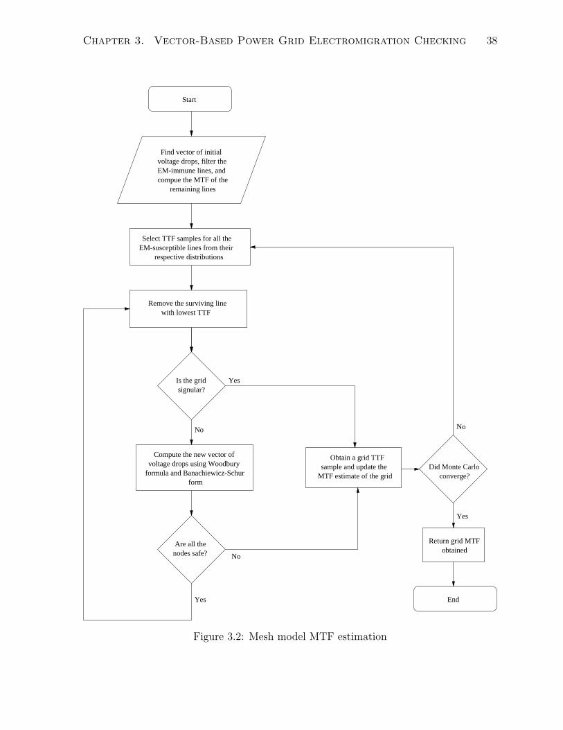
Chapter 3. Vector-Based Power Grid Electromigration Checking 38
signular?Is the grid
Are all the nodes safe?
Did Monte Carlo converge?
Start
Return grid MTF obtained
End
Yes
Yes
Yes
NoNo
No
Select TTF samples for all the
respective distributionsEM-susceptible lines from their
Remove the surviving line with lowest TTF
voltage drops, filter theEM-immune lines, andcompue the MTF of the
remaining lines
Find vector of initial
sample and update theMTF estimate of the grid
Obtain a grid TTF Compute the new vector ofvoltage drops using Woodbury
formformula and Banachiewicz-Schur
Figure 3.2: Mesh model MTF estimation

Chapter 3. Vector-Based Power Grid Electromigration Checking 39
Procedure 1 FIND VK
Input: V0, G0, uk, Zk−1, W−1k−1, xk−1, yk−1, k
Output: Vk, Zk, W−1k , xk, yk, grid singular
1: zk ← G−10 uk using LU factorization followed by backward forward substitutions.
2: pk ← uTk V03: if k = 1 then
4: Zk ← [zk]5: yk ← [pk]6: W−1
k ← 11−uT
kzk
7: xk ←W−1k yk
8: else
9: Zk ← [Zk−1 zk]10: yk ← [yTk−1 pk]
T
11: Find bk and dk as given in (3.24) and (3.25)12: Wb ←W−1
k−1bk13: sk ← dk − bTkWb
14: if sk = 0 then
15: grid singular ← 116: else
17: ak ← bTkxk−1−pk
sk18: Find xk using (3.31)19: Find Wk using (3.26)20: end if
21: end if
22: Vk ← V0 − Zkxk
the number of times the grid is found to survive up to t = Y (success). For a particular trial,
checking for a success can be done easily using Algorithm 1. In fact, computing the survival
probability for different values of Y allows us to derive the reliability function as well as other
statistical measures (PDF, CDF, and failure rate).
3.6 Experimental Results
Algorithms 1 and Procedure 1 have been implemented in C++. We carried out several ex-
periments using 5 different power grids generated as per user specifications, including grid
dimensions, metal layers, pitch and width per layer. Supply voltages and current sources were
randomly placed on the grid which is assumed to have Aluminum interconnects. The param-
eters of the grids are consistent with 1.1V 65nm CMOS technology. As for the EM model
employed, and because Aluminum is assumed, we use an activation energy of 0.9eV , a current
exponent η = 1 (we assume that the lifetime is dominated by the time taken by the void to
grow), a nominal temperature Tm = 373K (The user can provide any temperature profile for
the grid lines; we use Tm = 373 as an average temperature throughout the chip), a critical Blech
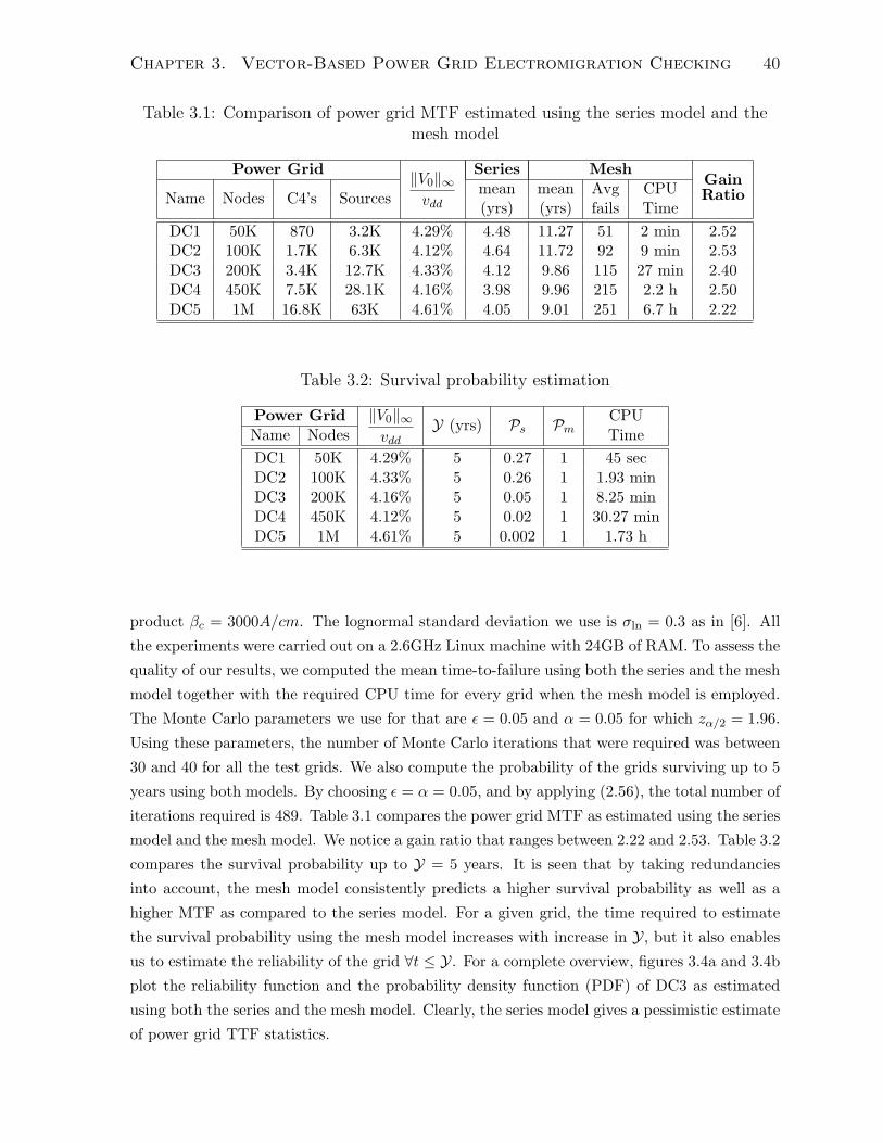
Chapter 3. Vector-Based Power Grid Electromigration Checking 40
Table 3.1: Comparison of power grid MTF estimated using the series model and themesh model
Power Grid ‖V0‖∞vdd
Series MeshGainRatioName Nodes C4’s Sources
mean mean Avg CPU(yrs) (yrs) fails Time
DC1 50K 870 3.2K 4.29% 4.48 11.27 51 2 min 2.52DC2 100K 1.7K 6.3K 4.12% 4.64 11.72 92 9 min 2.53DC3 200K 3.4K 12.7K 4.33% 4.12 9.86 115 27 min 2.40DC4 450K 7.5K 28.1K 4.16% 3.98 9.96 215 2.2 h 2.50DC5 1M 16.8K 63K 4.61% 4.05 9.01 251 6.7 h 2.22
Table 3.2: Survival probability estimation
Power Grid ‖V0‖∞vdd
Y (yrs) Ps Pm CPUName Nodes Time
DC1 50K 4.29% 5 0.27 1 45 secDC2 100K 4.33% 5 0.26 1 1.93 minDC3 200K 4.16% 5 0.05 1 8.25 minDC4 450K 4.12% 5 0.02 1 30.27 minDC5 1M 4.61% 5 0.002 1 1.73 h
product βc = 3000A/cm. The lognormal standard deviation we use is σln = 0.3 as in [6]. All
the experiments were carried out on a 2.6GHz Linux machine with 24GB of RAM. To assess the
quality of our results, we computed the mean time-to-failure using both the series and the mesh
model together with the required CPU time for every grid when the mesh model is employed.
The Monte Carlo parameters we use for that are ǫ = 0.05 and α = 0.05 for which zα/2 = 1.96.
Using these parameters, the number of Monte Carlo iterations that were required was between
30 and 40 for all the test grids. We also compute the probability of the grids surviving up to 5
years using both models. By choosing ǫ = α = 0.05, and by applying (2.56), the total number of
iterations required is 489. Table 3.1 compares the power grid MTF as estimated using the series
model and the mesh model. We notice a gain ratio that ranges between 2.22 and 2.53. Table 3.2
compares the survival probability up to Y = 5 years. It is seen that by taking redundancies
into account, the mesh model consistently predicts a higher survival probability as well as a
higher MTF as compared to the series model. For a given grid, the time required to estimate
the survival probability using the mesh model increases with increase in Y, but it also enables
us to estimate the reliability of the grid ∀t ≤ Y. For a complete overview, figures 3.4a and 3.4b
plot the reliability function and the probability density function (PDF) of DC3 as estimated
using both the series and the mesh model. Clearly, the series model gives a pessimistic estimate
of power grid TTF statistics.
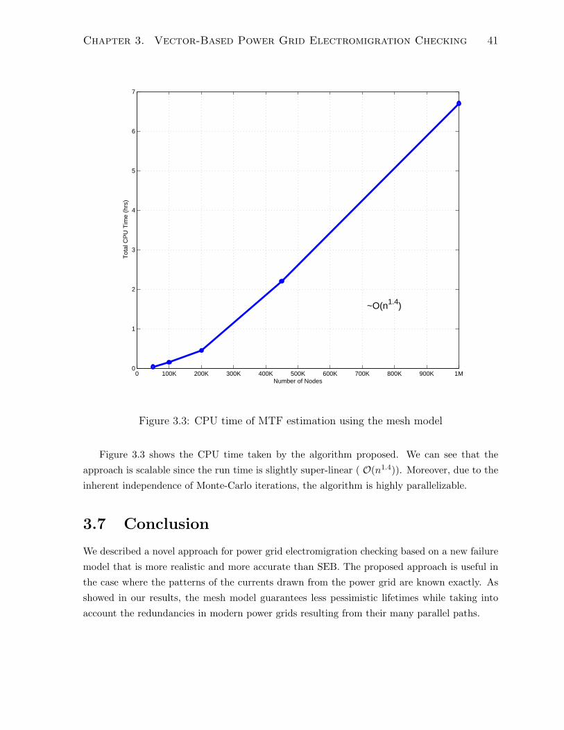
Chapter 3. Vector-Based Power Grid Electromigration Checking 41
0 100K 200K 300K 400K 500K 600K 700K 800K 900K 1M0
1
2
3
4
5
6
7
Number of Nodes
Tot
al C
PU
Tim
e (h
rs)
~O(n1.4)
Figure 3.3: CPU time of MTF estimation using the mesh model
Figure 3.3 shows the CPU time taken by the algorithm proposed. We can see that the
approach is scalable since the run time is slightly super-linear ( O(n1.4)). Moreover, due to the
inherent independence of Monte-Carlo iterations, the algorithm is highly parallelizable.
3.7 Conclusion
We described a novel approach for power grid electromigration checking based on a new failure
model that is more realistic and more accurate than SEB. The proposed approach is useful in
the case where the patterns of the currents drawn from the power grid are known exactly. As
showed in our results, the mesh model guarantees less pessimistic lifetimes while taking into
account the redundancies in modern power grids resulting from their many parallel paths.

Chapter 3. Vector-Based Power Grid Electromigration Checking 42
0 2 4 6 8 10 12 14 160
0.2
0.4
0.6
0.8
1
Time (years)
Rel
iabi
lity
Series ModelMesh Model
(a) Reliability function of grid DC3
0 2 4 6 8 10 12 14 160
0.02
0.04
0.06
0.08
0.1
Time (years)
Pro
babi
lity
Series ModelMesh Model
(b) Probability distribution function for TTFs of grid DC3
Figure 3.4: Estimated statistics for grid DC3 (200K nodes)

Chapter 4
Vectorless Power Grid
Electromigration Checking
4.1 Introduction
In chapter 3, we have seen how to estimate the reliability statistics of a power grid under the
effect of electromigration using the newly introduced mesh model. Recall that the currents
drawn from the power grid by the underlying logic blocks were assumed to be known exactly.
Clearly, if these currents change, the rate of EM degradation also changes. In practice, it is
not realistic to assume that the exact current waveforms are available for all the chip workload
scenarios, since this would require the simulation of the chip for millions of clock cycles at a low
enough level of abstraction that would provide the current waveforms. Moreover, one might
need to verify and check the grid early in the design flow, before fully designing the underlying
circuit. Therefore, one would like a vectorless approach that can deal with the uncertainty
about the underlying circuit currents. In this chapter, we present a vectorless extension of the
mesh model presented in the previous chapter. We show how the reliability statistics can be
obtained when only partial information about the power budget and the workload activity is
known.
4.2 Problem Definition
A constraint-based Vectorless power grid verification framework was first introduced in [27].
This framework defines a feasible space for currents in the form of current bounds, the idea
behind which is to capture circuit uncertainty via design specs or power budgets known in
the early design stages. Two types of constraints were defined: local constraints and global
constraints which respectively express bounds on the currents drawn by individual current
sources and by groups of current sources concurrently.
43

Chapter 4. Vectorless Power Grid Electromigration Checking 44
4.2.1 Modal Probabilities
Modern integrated circuits have complex multi-modal behavior, where major blocks of the chip
have different modes of operation (such as stand-by, low power, high performance, etc.). Spec-
ifying the block power dissipation requires knowledge of how often these modes are exercised.
For every circuit block j, let k = 1 . . . r enumerate the different modes of operation and Ijk
denote the block average supply current in that mode. The overall average supply current of
that block is given by Ij =r∑
k=1
αjkIjk, where 0 ≤ αjk ≤ 1 represent the probability of being in
different modes with the constraint thatr∑
k=1
αjk = 1. We propose that it is reasonable to expect
the user to specify the currents Ijk using the average power dissipation of each block in every
power mode. The mode probabilities αjk are generally harder to assess, but users are expected
to be able to specify values for some of them, or narrow ranges for others. If α denotes the
nr× 1 vector of all the mode probabilities (considering all the n blocks connected to the n grid
ndoes, having r modes of operation each), then we can write:
αmin ≤ α ≤ αmax (4.1)
where αmin and αmax have entries between 0 and 1, and contain any information the user may
have about the modes of operation. For a node with no current source attached, the lower and
upper bounds on its corresponding mode probabilities are set to zero.
The user can also specify bounds on the average current of every block, if available. This
allows us to infer other constraints on α in the form:
Iℓ,min ≤ Lα ≤ Iℓ,max (4.2)
where L is an n× nr matrix such that I = Lα. The matrix L contains information about the
currents drawn by the circuit blocks in each power mode.
Since chip components rarely draw their maximum currents simultaneously, global con-
straints are also used. For instance, if a certain limit is specified on the average power dissipa-
tion of the chip, then one may say that the sum of all the current sources is no more than a
certain upper bound. In general, the same concept can be applied for groups of current sources
forming functional blocks with known upper and lower bounds on their average power [27]. If
m is the total number of global constraints, then we can write:
Ig,min ≤ SLα ≤ Ig,max (4.3)
where S is an m × n matrix that only contains 0s and 1s and indicates which current sources
are present in each global constraint. The matrix contains a 1 at the kth entry of the ith row if

Chapter 4. Vectorless Power Grid Electromigration Checking 45
the kth circuit block (current sources) is present in the ith global constraint.
One last set of constraints should be added to guarantee that
r∑
k=1
αjk = 1 for every block j:
Bα = 1n (4.4)
where B is an n×nr matrix containing only 1s and 0s such that the vector Bα contains the sum
of mode probabilities per block in each of its entries. Together, all the constraints presented
above define a feasible space of mode probabilities, denoted by Fα, such that α ∈ Fα if and
only if, α satisfies (4.1) , (4.2), (4.3), and (4.4).
For example, consider a circuit having three blocks with two modes of operation each: high
performance and low power. Assume that the blocks draw respectively 0.2A, 0.3A, and 0.25A on
average in high performance mode, and 0.1A, 0.2A, and 0.15A in low power mode. Also, let α11,
α21, and α31 denote the probabilities of the blocks being in high performance mode, and α12,
α22, and α32 the probabilities of being in low power mode. If the average currents of the blocks
are I1, I2, and I3, and if I =[
I1 I2 I3
]Tand α =
[
α11 α12 α21 α22 α31 α32
]T
then we can write:
I = Lα =
0.2 0.1 0 0 0 0
0 0 0.3 0.2 0 0
0 0 0 0 0.25 0.15
α
The following is a possible set of constraints that a user can specify:
0.1
0.2
0.2
0.3
0.6
0.1
≤ α ≤
0.7
0.6
0.5
0.9
0.9
0.9
0.11
0.21
0.17
≤ Lα ≤
0.18
0.29
0.24
[
0.35
0.4
]
≤ SLα =
[
1 1 0
0 1 1
]
Lα ≤[
0.41
0.48
]
Bα =
1 1 0 0 0 0
0 0 1 1 0 0
0 0 0 0 1 1
α =
1
1
1
For every feasible setting of α, the overall block average currents are different, and the
reliability of the power grid is correspondingly different.

Chapter 4. Vectorless Power Grid Electromigration Checking 46
4.2.2 Current Feasible Space
As a first step towards finding the worst-case TTF of the grid, we transform the feasible space
Fα to the current domain. This helps reduce the number of variables from nr to n, as well as
the number of constraints. It is easy to see that replacing Lα by I in (4.2) and (4.3) results in
the first set of constraints defining the feasible space of currents:
Iℓ,min ≤ I ≤ Iℓ,max (4.5)
Ig,min ≤ SI ≤ Ig,max (4.6)
On the other hand, given the constraints on the individual α’s for every current source, we can
find lower and upper bounds for all the sources, as follows. Recall that every current source Ij
can be written as Ij =∑r
k=1 αjkIjk, and let αj denote the vector of all the mode probabilities
corresponding to Ij , then due to (4.1) we can write:
αj,min ≤ αj ≤ αj,max
where αj,min and αj,max contain the upper and lower bounds on the entries of αj as specified
in (4.1). Due to (4.4), we can write:∑r
k=1 αjk = 1, and hence, we can find bounds Ij,min and
Ij,max on Ij by solving the following two linear programs (LP):
Min/Maxr∑
k=1
αjkIjk
subject to αj,min ≤ αj ≤ αj,maxr∑
k=1
αjk = 1
(4.7)
The LPs above should be solved for every current source in the power grid. If any of the
LPs turns out to be infeasible, then the user specifications are not consistent. Notice that
due to the structure of the LPs above, we do not need to use any of the classical LP solving
methods (simplex or interior point). In fact, the claim below shows how compute the solutions
directly. Assume, without loss of generality, that the modes of operation of block j are sorted
in decreasing order of their power consumption, i.e. Ij1 ≥ Ij2 ≥ . . . ≥ Ijr. Also, call αjk,min
and αjk,max, k = 1, . . . , r, the entries of the vectors αj,min and αj,max respectively.
Claim 1. Consider the largest h ≤ r for whichh−1∑
k=1
αjk,max ≤ 1. Then, the solution to the

Chapter 4. Vectorless Power Grid Electromigration Checking 47
maximization problem in (4.7) is:
αjk =
αjk,max for k = 1, . . . , h− 1
1−h−1∑
k=1
αjk for k = h
αjk,min for k = h+ 1, . . . , r
Proof. To see why this works, notice that the problem is infeasible if∑r
k=1 αjk,min > 1 or∑r
k=1 αjk,max < 1. Assuming that the problem is feasible, we notice that we can replace the
last equality constraint by the inequality constraint∑r
k=1 αjk ≤ 1 without changing the optimal
solution. The reason is that if we were able to fit all the α’s without reaching equality, then∑r
k=1 αjk,max < 1, making the original problem infeasible, which contradicts our assumption.
Accordingly, we want to show that the greedy approach explained above solve the problem
below:
Maximize
r∑
k=1
αjkIjk
subject to αj,min ≤ αj ≤ αj,maxr∑
k=1
αjk ≤ 1
Consider the following transformation of variables:
wk =αjk − αjk,min
αjk,max − αjk,min, for k = 1, . . . , r
In the space of w, the problem becomes:
Maximizer∑
k=1
ckwk +r∑
k=1
Ijkαjk,min
subject to 0 ≤ wk ≤ 1, k = 1, . . . , rr∑
k=1
bkwk ≤ d
(4.8)
where ck = Ijk(αjk,max −αjk,min), bk = (αjk,max −αjk,min), and d = 1−∑rk=1 αjk,min. Because
the original problem is assumed to be feasible, we have d ≥ 0. Also, we notice that ck ≥ 0 and
bk ≥ 0 for every k. Ignoring the constant term∑r
k=1 Ijkαjk,min in the objective function, (4.8)
becomes an LP relaxation of the well known 0-1 Knapsack problem [28] for which the optimal
solution can be found using a greedy approach. If c1b1≥ c2
b2≥ . . . ≥ cr
br(which is true because
ck
bk= Ijk and the Ijk’s are assumed to be sorted in this order), then the optimal solution can be
found as follows: set w1 = w2 = . . . = wh−1 = 1, wh = d−∑h−1k=1 bk, and wh+2 = . . . = wr = 0,
where h is the largest possible. Transforming this solution back into the α space gives the
solution described earlier.

Chapter 4. Vectorless Power Grid Electromigration Checking 48
Claim 2. Consider the smallest g ≥ 1 for which
r∑
k=g+1
αjk,max ≤ 1. Then, the solution to the
minimization problem in (4.7) is:
αjk =
αjk,max for k = g + 1, . . . , r
1−r∑
k=g+1
αjk for k = g
αjk,min for k = 1, . . . , g − 1
The proof the claim 2 is similar to the proof of claim 1.
Ultimately if all the LPs turn out to be feasible, we obtain a lower and an upper bound on
every current source. However, (4.5) also provides similar bounds, hence, all the bounds should
be combined to obtain:
Imin ≤ I ≤ Imax (4.9)
Overall, we obtain a new feasible space of currents, that we call F , such that I ∈ F if and only
if, I satisfies (4.9) and (4.6).
Back to the example in the previous section, the resulting reduced set of constraints in the
current domain would be:
0.14
0.22
0.21
≤ I ≤
0.17
0.25
0.24
[
0.35
0.4
]
≤ SI =
[
1 1 0
0 1 1
]
I ≤[
0.41
0.48
]
Our goal is to look for the worst-case reliability of the power grid given all the possible feasible
combinations of I. For that, one can look into finding the worst-case MTF of the grid, or
the average worst-case TTF. Because our original vector-based engine uses Monte Carlo and
computes one grid TTF at a time, we will follow this up by also using a Monte Carlo approach
while computing a worst-case TTF of the grid, in every iteration, given all the constraints,
and finally report the average of all the obtained TTFs. This approach makes sense because
one would want to look into several samples of the grid and obtain the worst-case TTF for
each sample, and finally generate an average of all the minimums obtained. This leads to a
framework that allows vectorless EM checking while imposing reasonable and minimal demands
on the user.
4.3 Optimization
Over all the feasible vectors I ∈ F , we would like to find the average worst-case TTF of the grid,
which we do by performing a Monte Carlo analysis as before. In every iteration, we choose a
sample from the standard normal distribution for every line in the grid, and we find the smallest

Chapter 4. Vectorless Power Grid Electromigration Checking 49
grid TTF that can be obtained using the mesh model given any I ∈ F , and the set of samples
chosen for the lines. Recall that these samples are used to sample failure times for the lines
using equation (3.6) which in this case yields an expression for every TTF since I is not fixed.
Define Ψ to be the vector containing the samples ψl, l = 1 . . . b, and let T (Ψ, I) be a function
defined on F such that for every vector I ∈ F , T (Ψ, I) is the grid failure time corresponding
to the set of samples in Ψ and subject to the vector of source currents I. If Ψi represents the
vector containing the samples chosen at Monte Carlo iteration i, then the goal is to solve the
following set of optimization problems:
While (Monte-Carlo has not converged) :
Minimize: T (Ψi, I)
subject to: I ∈ F(4.10)
In the following, we discuss how to solve every minimization problem in the loop above given
a fixed vector Ψ. We do that by partitioning the feasible space into small subsets in which we
perform local optimizations. The global optimum will be the smallest of all the local optimums.
We first explain the local optimization in the first subset given a starting point in the feasible
space, and then show how to move into the other subsets.
4.3.1 Local Optimization
In this section, we will refer to T (Ψ, I) by T (I) for convenience. Let I(1) be a given point in
F and T (I(1)) be the corresponding grid time-to-failure. As will be explained later, we need
several initial points in F to solve every iteration in (4.10), and every initial point will lead to
a subset of F in which a local optimization will be performed. Therefore, a superscript is used
to index the initial points that will be chosen, as well as the corresponding subsets.
In order to compute T (I(1)), we need to compute the JL product of every line, filter
out all the lines that turn out to be EM-immune, and sort the other lines according to their
time-to-failure. Let l(1)1 , l
(1)2 , . . . , l
(1)ζ be the resulting sorted list of EM-susceptible lines, and
τ(1)1 , τ
(1)2 , . . . , τ
(1)ζ the corresponding list of TTFs such that:
τ(1)1 ≤ τ (1)2 ≤ . . . ≤ τ (1)ζ (4.11)
Also, let l(1)ζ+1, l
(1)ζ+2, . . . , l
(1)b be the list of all the other lines, i.e. the EM-immune ones.
Assume that, according to the order in (4.11), the grid fails for the first time after the
failure of the first p EM-susceptible lines. In other words, the grid is safe if l(1)1 , l
(1)2 , . . . , l
(1)p−1
fail, but fails when l(1)p fails. This implies that T (I(1)) = τ
(1)p as explained in the previous
chapter. Throughout the rest of this chapter, we assume that p < ζ, because otherwise, the
grid becomes immortal indefinitely which is unrealistic.

Chapter 4. Vectorless Power Grid Electromigration Checking 50
General Case
Definition 3. We define S(1) to be the subset of F corresponding to I(1) such that, at every
I ∈ S(1), the set of lines that fail until the failure time of the grid, their branch current directions,
the line that ultimately causes the grid to fail, and the EM-immune lines, are all the same as
those at I(1).
If, at any given point I ∈ S(1), the list of lines that fail before the failure of the grid is
l(I)1 , . . . , l
(I)p (in this order), the set of lines that are EM-susceptible but do not fail before the
failure of the grid is {l(I)p+1, . . . , l(I)ζ }, and the set of EM-immune lines is {l(I)ζ+1, . . . , l
(I)b }, then
we know, from the definition, that {l(I)1 , . . . , l(I)p } = {l(1)1 , . . . , l
(1)p }, l(I)p = l
(1)p , {l(I)p+1, . . . , l
(I)ζ } =
{l(1)p+1, . . . , l(1)ζ }, and {l
(I)ζ+1, . . . , l
(I)b } = {l
(1)ζ+1, . . . , l
(1)b }. Clearly, I(1) belongs to S(1) as all of the
conditions explained in the definition are satisfied.
For I ∈ F , assume that the TTF of line l(I)i , i ∈ {1, . . . , ζ}, can be written using (3.6) as:
τi(I) = |cTi I|−η
Let ξi = ±1 denote the sign of cTi I(1) for i ∈ {1, . . . , p}, i.e. ξi =
cTi I(1)
|cTi I(1)|, which implies
ξicTi I
(1) ≥ 0.
Claim 3. For every I ∈ S(1), T (I) = τp(I)
Proof. For any I ∈ S(1), l(I)p fails right after the failure of the set {l(I)1 , . . . , l(I)p−1} and is the first
to cause the failure of the grid. Therefore, T (I) = τp(I).
Claim 3 shows how to write T (I) as a closed form expression inside S(1) which is a non-empty
subset because I(1) ∈ S(1). To minimize T in F , we start by performing a local optimization in
a subset of F where T can be explicitly defined, namely S(1). In other words, we are interested
in solving the following optimization problem:
Minimize τp(I)
subject to I ∈ S(1)(4.12)
To solve (4.12), we introduce a new function νp on S(1) defined by νp(I) = (τp(I))− 1
η . Because
ξpcTp I
(1) ≥ 0, and because the direction of the current in line l(I)p (= l
(1)p ) is the same at both
I(1) and any I ∈ S(1), we have that ξpcTp I ≥ 0, ∀I ∈ S(1). Therefore, we can write νp(I) =
(τp(I))− 1
η =[
∣
∣cTp I∣
∣
−η]− 1
η=∣
∣cTp I∣
∣ = ξpcTp I, meaning, νp(I) is a linear function.
Lemma 1. A point Iopt is a solution for (4.12) if, and only if, νp(Iopt) is a maximum for νp(I)
in S(1).

Chapter 4. Vectorless Power Grid Electromigration Checking 51
Proof. Since η > 0 and τp(I) is a positive function for I ∈ S(1) (meaning νp(I) is a positive
function in S(1) as well), then:
Iopt is a solution for (4.12)⇔ τp(I) ≥ τp(Iopt), ∀I ∈ S(1)
⇔ (νp(I))−η ≥ (νp(Iopt))
−η, ∀I ∈ S(1)
⇔[
(νp(I))−η]− 1
η ≤[
(νp(Iopt))−η]− 1
η , ∀I ∈ S(1)
⇔ νp(I) ≤ νp(Iopt), ∀I ∈ S(1)
which proves the lemma.
Lemma 1 implies that in order to solve (4.12), we can solve instead the following maximiza-
tion problem
Maximize ξpcTp I
subject to I ∈ S(1)(4.13)
to get Iopt. The solution to (4.12) would simply be (ξpcTp Iopt)
−η.
For i ∈ {1, . . . , b}, let bi denotes the row of −R−1MTG−10 (from equation (2.33)) that
corresponds to line l(I)i , and let ai and Li denote the cross sectional area and length of l
(I)i
respectively. Also, define Gp to be the conductance matrix of the grid after the failure of
l(I)1 , . . . , l
(I)p , and Gp−1 the conductance matrix after the failure of l
(I)1 , . . . , l
(I)p−1 only. For now,
we assume that the failure occurs due to the violation of the voltage drop condition. The case
of failure by singularity is discussed later.
Theorem 1. I ∈ S(1) if, and only if, the following constraints are satisfied:
Li
aiξib
Ti I ≥ βc for i ∈ {1, . . . , p} (4.14)
Li
ai|bTi I| < βc for i ∈ {ζ + 1, . . . , b} (4.15)
ξpcTp I − ξicTi I ≤ 0 for i ∈ {1, . . . , p− 1} (4.16)
|cTi I| − ξpcTp I ≤ 0 for i ∈ {p+ 1, . . . , ζ} (4.17)
G−1p−1I ≤ Vth (4.18)
G−1p I 6≤ Vth (4.19)
Proof. Using definition 3, we know that for every I ∈ S(1), lines l(I)1 , . . . , l(I)p have the same
direction they have at I(1), therefore:
ξibTi I ≥ 0 and ξic
Ti I ≥ 0 for j ∈ {1, . . . , p} (4.20)
Also, lines l(I)1 , . . . , l
(I)p are EM-susceptible, meaning their JL products are greater than βc.

Chapter 4. Vectorless Power Grid Electromigration Checking 52
Using (3.2), this can be written as:
|bTi I|ai
Li ≥ βc, i = 1, . . . , p (4.21)
Similarly, lines l(I)ζ+1, . . . , l
(I)b are EM-immune, meaning we can write:
|bTi I|ai
Li < βc, i = ζ + 1, . . . , b
which is identical to (4.15).
Moreover, l(I)p fails after lines {l(I)1 , . . . , l
(I)p−1}, and before all the other lines. This is equivalent
to:
maxj∈{1,...,p−1}
τj(I) ≤ τp(I) ≤ mink∈{p+1,...,ζ}
τk(I)
which is also equivalent to:
maxj∈{1,...,p−1}
|cTj I|−η ≤ |cTp I|−η ≤ mink∈{p+1,...,ζ}
|cTk I|−η (4.22)
The grid is safe after the failure of the lines in the set {l(I)1 , . . . , l(I)p−1}. This is equivalent to (4.18)
because Gp−1 is defined to be the conductance matrix of the grid after the failure of those lines.
The grid fails after the failure of the lines in the set {l(I)1 , . . . , l(I)p }. This is equivalent to (4.19)
because Gp is defined to be the conductance matrix of the grid after the failure of those lines.
It remains to show that:
(4.20), (4.21), and (4.22)⇔ (4.14), (4.16), and (4.17)
We do this using a two way proof. Assume (4.20), (4.21), and (4.22) are true, then (4.21)
implies (4.14) because |bTi I| = ξibTi I for i = 1, . . . , p. Also, (4.22) implies:
maxj∈{1,...,p−1}
(
ξjcTj I)−η ≤
(
ξpcTp I)−η ≤ min
k∈{p+1,...,ζ}|cTk I|−η (4.23)
By taking the(
− 1η
)thpower of all the terms of (4.23), we can write
maxk∈{p+1,...,ζ}
|cTk I| ≤ ξpcTp I ≤ minj∈{1,...,p−1}
ξjcTj I (4.24)
which implies (4.16) and (4.17). This is true because − 1η < 0 and hence, taking the
(
− 1η
)th
power reverses all the inequalities in which case, the min operator becomes a max, and vice
versa.
On the other hand, assume (4.14), (4.16), and (4.17) are true, then (4.24) is true. Since

Chapter 4. Vectorless Power Grid Electromigration Checking 53
maxk∈{p+1,...,ζ}
|cTk I| ≥ 0, then
0 ≤ ξpcTp I ≤ minj∈{1,...,p−1}
ξjcTj I
and hence, (4.20) is true. In addition, we can take the (−η)th power of all the terms in (4.24)
to get (4.23) because −η < 0. Now, we can easily get (4.22) from (4.23) because (4.20) is true.
Finally, (4.21) is also true because of (4.20) and (4.14).
Notice that (4.15) is equivalent to:
Li
aibTi I < βc and − Li
aibTi I < βc for i ∈ {ζ + 1, . . . , b} (4.25)
which can be written in matrix form as
H1I < h1 (4.26)
where H1 is a 2(b− ζ)× n matrix and whose rows are the row vectors
Li
aibTi and − Li
aibTi , i ∈ {ζ + 1, . . . , b}
Call γ1 the number of rows in H1 (γ1 = 2(b − ζ)). The vector h1 is the vector of size γ1
containing βc in all its entries.
Similarly, the inequalities in (4.14), (4.16), (4.17), and (4.18) can be combined in matrix
form as
H2I ≤ h2 (4.27)
with H2 being the (n+ 2ζ − 1)× n matrix whose rows are the row vectors
−Li
aiξib
Ti , i ∈ {1, . . . , p}
ξpcTp − ξicTi , i ∈ {1, . . . , p− 1}
cTi − ξpcTp and − cTi − ξpcTp , i ∈ {p+ 1, . . . , ζ}
and the rows of G−1p . Call γ2 the number of rows in H2 (γ2 = n+ 2ζ − 1). The vector h2 is of
size γ2 and is the following:
h2 =
−βc1p02ζ−p−1
Vth

Chapter 4. Vectorless Power Grid Electromigration Checking 54
Ultimately, S(1) can be redefined using the following set of constraints:
I ∈ FH1I < h1
H2I ≤ h2
G−1p I 6≤ Vth
All the constraints presented above are linear and define a convex polytope (or the interior of
a convex polytope) except G−1p I 6≤ Vth which consists of a disjunction of constraints where at
least one entry of G−1p I has to be greater than its corresponding entry in Vth. We deal with
that using a theorem that will be presented shortly.
For any strictly positive number δ define a fixed real number d = ‖Vth‖∞(1 + δ).
Theorem 2. For any I, G−1p I 6≤ Vth if and only if, ∃y ∈ {0, 1}n with ‖y‖1 ≤ n − 1 such that
G−1p I > Vth − dy.
Proof. If G−1p I 6≤ Vth, then there exists a non-empty set of indices K ⊆ {1, . . . , n} such that
eTkG−1p I > eTk Vth for every k ∈ K. If we let y = [y1 . . . yn]
T with yk = 0 for k ∈ K, and yk = 1
otherwise, then clearly ‖y‖1 ≤ n− 1, and G−1p I > Vth− dy because d > ‖Vth‖∞ and the entries
of the vector G−1p I are always positive.
On the other hand, if there exists y ∈ {0, 1}n with ‖y‖1 ≤ n − 1, and G−1p I > Vth − dy,
then ∃k such that yk = 0, and eTkG−1p I > eTk Vth. Therefore, G
−1p I 6≤ Vth.
The theorem above allows rewriting (4.13) as follows:
Maximize ξpcTp I
subject to I ∈ FH1I < h1
H2I ≤ h2
G−1p I > Vth − dy‖y‖1 ≤ n− 1
y ∈ {0, 1}n
(4.28)
The problem above is an integer linear program (ILP) because it has a linear objective function,
linear constraints, and some integer variables, namely the entries of y; solving this ILP would
solve (4.12) as explained before, and would minimize T inside S(1) ⊂ F .
Singular Case
If at I(1) the grid fails by singularity, then the same analysis as above can be done. The only
difference is that the constraint G−1p I 6≤ Vth cannot be added, and is in fact redundant because

Chapter 4. Vectorless Power Grid Electromigration Checking 55
(2)
F
S(1)
I
I
(1)
Figure 4.1: Choosing the next starting point I(2)
Gp is known to be singular in this case, and there is no need to add that as one of the constraints
defining S(1). Notice that in this case, (4.13) becomes a linear program:
Maximize ξpcTp I
subject to I ∈ FH1I < h1
H2I ≤ h2
(4.29)
In the following, we show how to globally minimize T in F by performing a set of local
optimizations as above until F is fully explored.
4.3.2 Exact Global Optimization
Similarly to S(1), every local optimization requires a starting point in F . In order to create S(2),we need a point I(2) ∈ F at which we compute the TTF of the grid and then follow a similar
procedure to the one explained in the previous section. Note that finding I(1) can be done
by solving a linear feasibility problem in the set F . However, we cannot do the same for I(2)
because if we choose I(2) in F without other restrictions and it turns out that it belongs to S(1),then S(2) becomes identical to S(1), which adds redundancy to our approach and accordingly,
the global optimization may or may not terminate. In short, I(2) should be chosen in the set
F −S(1) (See figure 4.1). Using the constraints in theorem 1, we can infer the set of conditions

Chapter 4. Vectorless Power Grid Electromigration Checking 56
required for I(2) to be in outside S(1) (in the general case) as follows:
H1I 6< h1
or H2I 6≤ h2
or G−1p I ≤ Vth
(4.30)
For any strictly positive number δ, define
d = (1 + δ)max(
‖h1 −H1I‖∞, ‖h2 −H2I‖∞, ‖G−1p I − Vth‖∞
)
Theorem 3. (4.30) is true if and only if, there exists x ∈ {0, 1}γ1, y ∈ {0, 1}γ2, and z ∈ {0, 1}with
‖x‖1 + ‖y‖1 + z ≤ γ1 + γ2 (4.31)
such that:H1I ≥ h1 − dxH2I > h2 − dy
G−1p I ≤ Vth + dz1n
(4.32)
Proof. The proof is similar to that of theorem 2. Assume (4.30) is true, and define x =
[x1 . . . xγ1 ]T , y = [y1 . . . yγ2 ]
T , and z, such that:
xk = 0 ⇐⇒ eTkH1I ≥ eTk h1, for k = 1, . . . , γ1
yk = 0 ⇐⇒ eTkH2I > eTk h2, for k = 1, . . . , γ2
z = 0 ⇐⇒ G−1p I ≤ Vth
Also, let v = [xT yT z]T . Because (4.30) is true, then at least one entry in v is zero, since
otherwise, we have that H1I < h1, H2I ≤ h2, and G−1p 6≤ Vth, which makes (4.30) false. Having
at least one zero entry in v means that there exists a nonempty set of indices K ⊆ {1, . . . , γ1 +γ2+1} such that vk = 0 for k ∈ K. Clearly, (4.31) is true because ‖x‖1+‖y‖1+z = ‖v‖1 ≤ γ1+γ2.We still have to check that (4.32) is true.
1. Define K1 = K ∩ {1, . . . , γ1}. We will first show that
H1I ≥ h1 − dx (4.33)
i.e. eTkH1I ≥ eTk h1 − dxk for k ∈ {1, . . . , γ1}. If k ∈ K1, then we know eTkH1I > eTk h1,
meaning eTkH1I > eTk h1 − dxk (because xk = 0). If k ∈ {1, . . . , γ1} − K1, then eTkH1I >
eTk h1 − dxk because xk = 1, and d > ‖h1 −H1I‖∞ (i.e. d ≥ eTk (h1 −H1I) for every k).
2. Define K′2 = K ∩ {γ1 + 1, . . . , γ1 + γ2}, and K2 = {k − γ1 : k ∈ K′
2}. We will now show
that
H2I > h2 − dy (4.34)
Chapter 4. Vectorless Power Grid Electromigration Checking 57
i.e. eTkH2I > eTk h2 − dyk for k ∈ {1, . . . , γ2}. If k ∈ K2, then we know eTkH2I > eTk h2,
meaning eTkH2I > eTk h2 − dyk (because yk = 0). If k ∈ {1, . . . , γ2} − K2, then eTkH2I >
eTk h2 − dyk because yk = 1, and d > ‖h2 −H2I‖∞ (i.e. d > eTk (h2 −H2I) for every k).
3. We will finally show that:
G−1p I ≤ Vth + dz1n (4.35)
i.e. eTkG−1p I ≤ eTk Vth + dz for k ∈ {1, . . . , n}. If z = 0, then we know G−1
p I ≤ Vth which
means that (4.35) is automatically true. If z = 1, then eTkG−1p I ≤ eTk Vth+ dz is true (and
so is (4.35)) because d > ‖G−1p I − Vth‖∞ (i.e. d ≥ eTk (G−1
p I − Vth) for every k).
We now prove the other direction of the theorem. Assume that there exists x ∈ {0, 1}γ1 ,y ∈ {0, 1}γ2 , and z ∈ {0, 1} with (4.31) and (4.32) being true, then either z = 0, or ∃k such that
xk = 0 or ∃k such that yk = 0. If z = 0, then G−1p I ≤ Vth, and if xk = 0, then eTkH1I > eTk h1
and if yk = 0 then eTkH2I > eTk h2, which basically implies (4.30).
In the singular case, the last set of constraints in (4.32) as well as the binary variable z are
not needed. Theorem 3 implies that finding I(2) requires solving a feasibility problem in the
following space:
I ∈ FH1I ≥ h1 − dxH2I > h2 − dy
G−1p I ≤ Vth + dz1n
‖x‖1 + ‖y‖1 + z ≤ γ1 + γ2
x ∈ {0, 1}γ1 , y ∈ {0, 1}γ2 , z ∈ {0, 1}
which can be done using an ILP. The same approach should be used to find the ith starting
point corresponding to subset S(j): I(i) should be chosen as to satisfy the constraints I ∈ Fand I 6∈ S(j), j = 1, . . . , i− 1. This can also be done using an ILP similarly to I(2). When such
point cannot be found, i.e. when F −⋃i−1j=1 S(j) becomes empty, we infer that the feasible space
F is fully explored and the algorithm terminates while returning the best local minimum found.
The result is one sample TTF for the grid which should be added to the other samples found
in other Monte Carlo iterations. Algorithm 2 shows how to compute exact global minimum of
the grid TTF given a set of normal samples Ψ using the proposed approach.
4.4 Experimental Results
Algorithm 2 has been implemented in C++. The algorithm use the Mosek optimization pack-
age [29] to solve the required LPs and ILPs. An approximate sparse inverse of G0 is found
using SPAI [30], and all the other required inverses are found using the Woodbury formula,
i.e. (3.14). We carried out several experiments using 5 different power grids generated as per

Chapter 4. Vectorless Power Grid Electromigration Checking 58
Algorithm 2 EXACT GLOBAL MINIMIZATION
Input: ΨOutput: Global Minimum of T (Ψ, I)1: Find I(1) in F using an LP2: Set solved← false and i← 23: while (solved = false) do4: Find T (Ψ, I(i−1)) using Algorithm 15: Build the constraints defining S(i−1) as outlined in section 4.3.16: Solve maxI∈S(i−1) T (I) using an ILP
7: Solve a feasibility problem in F −⋃i−1j=1 S(j) to get I(i) as outlined in section 4.3.2
8: if (I(i) cannot be found) then9: solved← true
10: end if
11: i← i+ 112: end while
13: Return the smallest local minimum found
Table 4.1: Exact average minimum TTF computation
Power Grid Proposed Approach
Name Nodes C4’s SourcesAvg Min CPUTTF (yrs) Time
G1 141 12 12 7.50 3.21 minG2 177 12 12 9.11 5.94 minG3 237 12 20 10.38 25.10 minG4 392 24 30 8.01 49.24 minG5 586 12 42 9.79 4.42 h
user specifications, including grid dimensions, metal layers, pitch and width per layer. Supply
voltages and current sources were randomly placed on the grid. The parameters of the grids
are consistent with 1.1V 65nm CMOS technology. As for the EM model employed, we use,
as before, an activation energy of 0.9eV , a current exponent η = 1, a nominal temperature
Tm = 373K, a critical Blech product βc = 3000A/cm, and a standard deviation σln = 0.3.
All the experiments were carried out on a 2.6GHz Linux machine with 24GB of RAM. We
compute the average minimum time-to-failure of the grid and report the required CPU time
for every grid. The Monte Carlo parameters we use for that are ǫ = 0.1 and α = 0.05 for which
zα/2 = 1.96. Table 4.1 shows the test grids with the number of nodes, the number of voltage
sources (C4s), and the number of current sources indicated in each case. The obtained average
minimum grid time-to-failure for each grid are reported. The CPU time required is reported
as well and is shown in figure 4.2. By investigating the runtime of the different parts of our
algorithm, it turns out that most of the total CPU time is spent on selecting starting points
required to generate the subsets. It should also be noted that the number of subsets that were

Chapter 4. Vectorless Power Grid Electromigration Checking 59
100 150 200 250 300 350 400 450 500 550 6000
0.5
1
1.5
2
2.5
3
3.5
4
4.5
Number of Nodes
Tot
al C
PU
Tim
e (h
rs)
Figure 4.2: CPU time of the exact approach versus the number of grid nodes
found in F is on average, between 20 and 40 subsets depending on the structure of the feasible
space as well as on the random seeds used for selecting the TTFs of the grid lines.
4.5 Conclusion
We described an early vectorless approach for power grid electromigration checking under a
constraint-based framework to capture workload uncertainty. We presented an exact, theo-
retically interesting approach which requires solving several ILPs. With proper parallelization
the exact optimization may become practical to check for electromigration in the main feeder
network or in parts of the whole grid, but for all practical purposes, the method is of theoretical
interest only and is not scalable.

Chapter 5
Simulated Annealing Based
Electromigration Checking
5.1 Introduction
As mentioned in chapter 4, vectorless electromigration checking is required to manage user
uncertainties about the chip workload. The approach we developed is exact, and is useful for
small grids. However, for large grids containing hundreds of thousands of nodes, the method
becomes impractical to use as it requires solving several ILPs in every Monte Carlo iteration.
In this chapter, we present three approximate approaches for constraint-based power grid elec-
tromigration checking. All the methods are based on Simulated Annealing, a heuristic based
global optimization technique. The first method uses the TTF estimation technique developed
in chapter 3 as well as the local optimizer developed in chapter 4. The second method uses the
TTF estimation technique developed in [24], which is an extension to our original estimation
technique (from chapter 3) and that takes care of changing branch currents as grid lines start to
fail. The third method uses an extension to the TTF estimation technique of [24], and explores
locality in the grid.
5.2 Simulated Annealing for Continuous Problems
5.2.1 Overview
Simulated Annealing (SA) is a random-search global optimization techniques that was first
developed by Kirkpatrick et al [31] and Cerny [32]. SA was found to be useful to solve many
VLSI CAD problems. SA is often used when the search space is discrete but can also be used for
continuous global optimization problems. In this chapter, we are concerned with optimization
over continuous variables as our feasible space is a continuous domain of currents, i.e. we are
60

Chapter 5. Simulated Annealing Based Electromigration Checking 61
concerned with problems having the following form:
f∗ = minx∈X
f(x) (5.1)
where X ⊆ Rn is a continuous compact domain. SA algorithms are based on an analogy with
annealing in metallurgy, a technique that involves cooling and heating a material as to increase
the size of its crystals and reduce their defects. If the temperature is slowly decreased, the
thermal mobility of the molecules is reduced and they form a pure crystal that corresponds to
the state of minimum energy. If the temperature is decreased quickly, a liquid metal rather
ends up in a polycrystalline or amorphous state with a higher energy and not in a pure crystal.
In [33], a Metropolis Monte Carlo method was proposed to simulate the physical annealing
process. Later, SA algorithms for combinatorial optimization problems were developed by
observing the analogies between the configurations of a physical system and the feasible points,
and between the energy function and the objective function. The approach has been later
extended to continuous global optimization problems.
5.2.2 Main Algorithm
At each iteration, SA algorithms generate a candidate point and decide whether to move to it
or to stay at the current point based on a random mechanism controlled by a parameter called
temperature. The flow of the algorithm is as follows:
• Step 0: Choose x0 ∈ X and let z0 = {x0} and k = 0.
• Step 1: Sample a point yk+1 from the next candidate distribution D(zk).
• Step 2: Sample a number p between 0 and 1 from the uniform distribution and set:
xk+1 =
{
yk+1 if p ≤ A(xk, yk+1, Tk)
xk otherwise(5.2)
where A is called the acceptance function and has values in [0, 1], and Tk is a parameter
called the temperature at iteration k.
• Step 3: Set zk+1 = zk ∪{yk+1}. The set zk contains all the information collected up to
iteration k, i.e. all the points observed up to this iteration.
• Step 4: Set Tk+1 = U(zk+1, T0), where U is called the cooling schedule and is a function
with nonnegative values.
• Step 5: Check a stopping criterion and if it fails, set k ← k + 1 and go back to step 1.

Chapter 5. Simulated Annealing Based Electromigration Checking 62
In order to define a complete SA algorithm, one should appropriately choose the distribution
D of the next candidate point, the acceptance function A, the cooling schedule U , and the
stopping criterion. Below, we present a short discussion about each component separately.
5.2.3 The Acceptance Function
Very few acceptance functions have been employed in the existing literature about SA for
continuous optimization problems. The acceptance function used in most cases is the Metropolis
function presented below:
A(x, y, T ) = min
{
1, exp
(
−f(y)− f(x)T
)}
(5.3)
Notice that the condition p ≤ A(xk, yk+1, Tk) in step 2 of the SA algorithm is automatically
satisfied if f(yk+1) ≤ f(xk) because in this case, A(xk, yk+1, Tk) = 1. Accordingly, xk+1 = yk+1.
In the case where f(yk+1) ≥ f(xk), the Metropolis function generates a number between 0 and
1 representing the probability of accepting the next candidate point yk+1. This probability
depends on the temperature parameter Tk and on how large is the gap |f(yk+1) − f(xk)|.Notice that, a large gap or a low temperature result in a low acceptance probability. Accepting
an ascent step from f(xk) to f(yk+1) is sometimes necessary to avoid being trapped at a local
minimum, and is called hill-climbing.
Another possible acceptance function is the Barker function:
A(x, y, T ) = 1
1 + exp(
f(y)−f(x)T
) (5.4)
Notice that the Barker function may not accept descent steps if they don’t improve the function
value by a significant amount. Nonetheless, at low T , descent steps are most likely accepted.
5.2.4 Cooling Schedule
An appropriate choice of the cooling schedule U is critical for a well performing SA algorithm.
Good cooling schedules generally depend on the value of f∗ (the optimal objective), in which
case the purpose of SA is finding a point x∗ ∈ X having a (near) optimal objective. In [34], the
cooling schedule is defined as follows:
U(zk, T0) = β [f(xk)− f∗]g1 (5.5)
where β, g1 > 0 are constants. If f∗ is not known, it is suggested to employ an estimate f of it
which is updated every time a function value lower than the estimate is found. The basic idea
of the schedule above is that ascent steps should be accepted with a low probability when the

Chapter 5. Simulated Annealing Based Electromigration Checking 63
function value at the current point xk is close to the global optimum. Instead, if the function
value at xk is much greater than the global optimum, the temperature is high and ascent steps
are accepted to prevent the algorithm from getting trapped away from the global optimum.
In the case where no estimate f can be obtained, one can simply use:
Tk+1 = a⌊ kM ⌋T0 (5.6)
where T0 is the initial temperature, a is a real number between 0.8 and 0.99, and M is an
integer. This cooling schedule allows the temperature to decrease by a factor of a after each
group of M iterations.
Notice that any cooling schedule must take into account the scale of the function in consid-
eration. For example, assume that Tk = 1, f(xk) = 0, and f(yk+1) = 0.1, then the probability
that xk+1 = yk+1 is equal to e−0.1 ≈ 0.9 (according to the Metropolis function). For another
function g(x) = 1000 × f(x), g(xk) = 0, and g(yk+1) = 100, and hence the probability that
xk+1 = yk+1 is equal to e−100 ≈ 0. Therefore, we notice how poorly the SA algorithm behaves
when the temperature does not take into account the scale of the function.
To solve this problem, one can compute the objective function at one or more points in
the feasible space. A good starting temperature would be 5-10 times larger than the observed
function values.
5.2.5 Next Candidate Distribution
Because the feasible space is a continuous domain, there are infinitely many possible next
candidate points. The point starting point x0 can be found by solving a feasibility problem
inside the space X (which can be done by solving an LP in the case where X is a convex
polytope). Choosing other points in X, however, must be done in a random and more efficient
way. In [34] the next candidate point yk+1 is generated as follows:
yk+1 = xk +∆rθk (5.7)
where θk is a random direction in Rn with ‖θk‖2 = 1, and ∆r is a fixed step size. If the point
obtained is outside X, another point is generated using the same procedure. The choice of ∆r
usually depends on the objective function f and on the volume of the feasible space, and bad
choices may lead to a deterioration of the performance of the algorithm. Moreover, when the
dimension n is high, the probability of obtaining a point inside the feasible space becomes low,
and one might need to repeat the procedure above many times before obtaining a point inside
X.
A better approach explained in [35] generates yk+1 by first choosing θk as above, and then
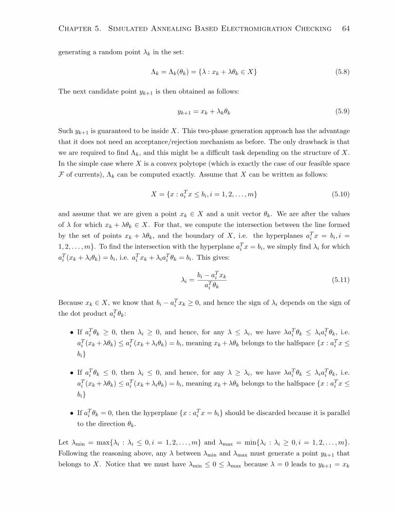
Chapter 5. Simulated Annealing Based Electromigration Checking 64
generating a random point λk in the set:
Λk = Λk(θk) = {λ : xk + λθk ∈ X} (5.8)
The next candidate point yk+1 is then obtained as follows:
yk+1 = xk + λkθk (5.9)
Such yk+1 is guaranteed to be inside X. This two-phase generation approach has the advantage
that it does not need an acceptance/rejection mechanism as before. The only drawback is that
we are required to find Λk, and this might be a difficult task depending on the structure of X.
In the simple case where X is a convex polytope (which is exactly the case of our feasible space
F of currents), Λk can be computed exactly. Assume that X can be written as follows:
X = {x : aTi x ≤ bi, i = 1, 2, . . . ,m} (5.10)
and assume that we are given a point xk ∈ X and a unit vector θk. We are after the values
of λ for which xk + λθk ∈ X. For that, we compute the intersection between the line formed
by the set of points xk + λθk, and the boundary of X, i.e. the hyperplanes aTi x = bi, i =
1, 2, . . . ,m}. To find the intersection with the hyperplane aTi x = bi, we simply find λi for which
aTi (xk + λiθk) = bi, i.e. aTi xk + λia
Ti θk = bi. This gives:
λi =bi − aTi xkaTi θk
(5.11)
Because xk ∈ X, we know that bi − aTi xk ≥ 0, and hence the sign of λi depends on the sign of
the dot product aTi θk:
• If aTi θk ≥ 0, then λi ≥ 0, and hence, for any λ ≤ λi, we have λaTi θk ≤ λiaTi θk, i.e.
aTi (xk+λθk) ≤ aTi (xk+λiθk) = bi, meaning xk+λθk belongs to the halfspace {x : aTi x ≤bi}
• If aTi θk ≤ 0, then λi ≤ 0, and hence, for any λ ≥ λi, we have λaTi θk ≤ λiaTi θk, i.e.
aTi (xk+λθk) ≤ aTi (xk+λiθk) = bi, meaning xk+λθk belongs to the halfspace {x : aTi x ≤bi}
• If aTi θk = 0, then the hyperplane {x : aTi x = bi} should be discarded because it is parallel
to the direction θk.
Let λmin = max{λi : λi ≤ 0, i = 1, 2, . . . ,m} and λmax = min{λi : λi ≥ 0, i = 1, 2, . . . ,m}.Following the reasoning above, any λ between λmin and λmax must generate a point yk+1 that
belongs to X. Notice that we must have λmin ≤ 0 ≤ λmax because λ = 0 leads to yk+1 = xk

Chapter 5. Simulated Annealing Based Electromigration Checking 65
| |X
λ
λ
xk
θk
max
min
λ
yk+1
|| |
Figure 5.1: Generating lambda
which belongs to X. Ultimately, the set Λk can be described as follows:
Λk = {λ : λmin ≤ λ ≤ λmax} (5.12)
The procedure above is illustrated in figure 5.1. Even though this two-phase mechanism
presents a huge advantage over the first approach, it still presents a major drawback known as
the jamming problem. Jamming occurs when the point xk is very close to a boundary of the
feasible region. In this case, the set Λk is very small along many directions θk. To see why,
consider a hypercube in Rn and assume that xk is very close to one of its corners. The fraction
of the whole set of directions leading to small set Λk is about 1− 12n (The only viable directions
are the ones away from the corner, and these roughly represent 12n of all the directions). When
the set Λk is small, the next candidate point will be very close to xk, and hence a small progress
will be observed in the algorithm. To solve this problem, the concept of reflection is introduced
in [36]. The basic idea of reflection consists of generating points outside X and reflect them
back into X. Let X be some compact set containing X. We define the set Λk as follows:
Λk = Λk(θk) = {λ : xk + λθk ∈ X} (5.13)
We then sample a uniform random point λk from Λk, and obtain the point:
yk+1 = xk + λkθk (5.14)

Chapter 5. Simulated Annealing Based Electromigration Checking 66
θθ
k
k
xk
yk +1
yk +1
X
X
y+1k
~
Figure 5.2: One way of reflecting yk+1 back into X to obtain yk+1 = yk+1
If yk+1 ∈ X, then we simply set yk+1 = yk+1 to obtain our next candidate point. Otherwise, we
reflect yk+1 back into X by first finding the point yk+1, intersection between the line segment
[xk, yk+1] and the boundary of X (which can be easily done as before when X is a convex
polytope), and then computing the point y′k+1 as follows:
y′k+1 = yk+1 + ‖yk+1 − yk+1‖θk (5.15)
where θk is a random vector in Rn with ‖θk‖ = 1. If y′k+1 ∈ X, then we set yk+1 = y′k+1,
otherwise, we reflect y′k+1 back into X. Figure 5.2 illustrates the procedure explained.
5.2.6 Stopping Criterion
Due to the difficult nature of the problems solved by SA algorithms, it is hard to define a
stopping criterion which guarantees a global optimum within a given accuracy. Typically, one
of the following rules is applied:
• A given minimum temperature has been reached.
• A certain number of iterations has passed without accepting a new solution.
• A specific number of total iterations has been executed.

Chapter 5. Simulated Annealing Based Electromigration Checking 67
5.3 Simulated Annealing with Local Optimization
As our first approximate approach, we propose using SA in the context of a Monte Carlo simu-
lation to find the average minimum grid TTF of the grid. We use SA to minimize the function
T (Ψi, I) (defined in section 4.3) over the feasible space F in every Monte-Carlo iteration. We
use the Metropolis function as our acceptance function, and use the cooling schedule in (5.6).
To sample random points in F , we use the two phase generation mechanism presented earlier
as well as reflection for a better space exploration. Our SA algorithm converges once the tem-
perature reaches a certain minimum value Tǫ. Once SA terminates, we run the local optimizer
we developed in section 4.3.1 at the best point found. However, instead of solving an ILP, we
solve a relaxed version by allowing the entries of the vector y (in (4.28)) to be in the range
[0, 1] instead of the set {0, 1}. The result is an estimate sample for the minimum grid TTF. As
before, enough samples should be collected until Monte Carlo converges. Algorithm 3 shows
the details of our first approximate approach to minimize the grid TTF given a set of normal
samples Ψ using SA and the local minimizer.
Algorithm 3 SIMULATED ANNEALING WITH LOCAL OPTIMIZATION
Input: ΨOutput: Global Minimum of T (Ψ, I)1: Find a starting point I0 in F using an LP2: Compute T (Ψ, I0) using Algorithm 13: Set k ← 0, and choose an initial temperature T0.4: while (Tk+1 ≥ ǫ) do5: Sample a new point I ′k+1 in F as explained in section 5.2.56: Find T (Ψ, I ′k+1) using Algorithm 17: Find Ik+1 based on the acceptance function (5.3) as in (5.2)8: Find Tk+1 using (5.6)9: Set k ← k + 1
10: end while
11: Solve a local minimization around the best point found using a convex relaxation of theILP and return the result (procedure of section 4.3.1).
5.4 Optimization with Changing Currents
5.4.1 Estimating EM Statistics for Step Currents
Recall (from section 3.3.3) that when developing the approach for estimating the EM statistics
of the power grid when the chip workload is known exactly, we assumed that the statistics of
the individual lines can be determined using the branch currents of the grid before the failure
of any of its components. This basically means that, as the grid lines start to fail, we ignore
the changes in the branch currents and the effect of these changes on the time-to-failure of

Chapter 5. Simulated Annealing Based Electromigration Checking 68
the lines. In [24], the authors developed an extension to this approach in which the change in
failure statistics is estimated when the current densities in the lines change over time. Below,
we summarize the key points in their approach.
Consider a specific metal line of length L in the power grid subject to the following current
density profile:
J(t) =
J0 for t0 ≤ t ≤ t1J1 for t1 < t ≤ t2...
Jk for tk < t ≤ tk+1
...
Jp for tp < t < tp+1
(5.16)
where Jk−1 6= Jk ∀k > 0, t0 = 0, and tp+1 = ∞. It is interesting to note that (5.16) is the
typical current density profile of a surviving interconnect in the power grid, where the kth
failing interconnect has τ = tk. Let Tk represent the random variable describing the statistics
of the line for the time span tk < t ≤ tk+1. The RV Tk is defined over [0,∞] but describes the
statistics of line only for t ∈ (tk, tk+1]. Let µT,k = E[Tk], and let τk represent the time-to-failure
sample of the line for the same time span tk < t ≤ tk+1. Under certain mild assumptions, and
ignoring the Blech effect, the authors show that the following holds:
(
µT,k
µT,k-1
)
=
(
Jk−1
Jk
)η
(5.17)
which then leads to the following formula to update the TTF sample of the line:
τk = tk + (τk−1 − tk−1)
(
Jk−1
Jk
)η
(5.18)
If the Blech effect is considered, then two cases arise. If JkL ≤ βc, then τk = ∞. Otherwise,
the formula to update the TTF sample becomes as follows:
τk = tk + (τk−q − tk−q+1)
(
Jk−q
Jk
)η
(5.19)
where q is such that Jk−qL > βc, JkL > βc, and JiL ≤ βc for i ∈ {k − q + 1, . . . , k − 1}.
In order to find the TTF of a grid using the changing currents model, the authors follow
the steps of Algorithm 4. They start with a list L of all the grid lines to which they assign TTF
samples (they assign ∞ to immortal lines). Every time a line fails, the TTF of the remaining
lines in L are updated as explained above. Procedure 1 of chapter 3 is also used to update the
voltage drops as before (Woodbury formula and Banachiewicz-Schur).
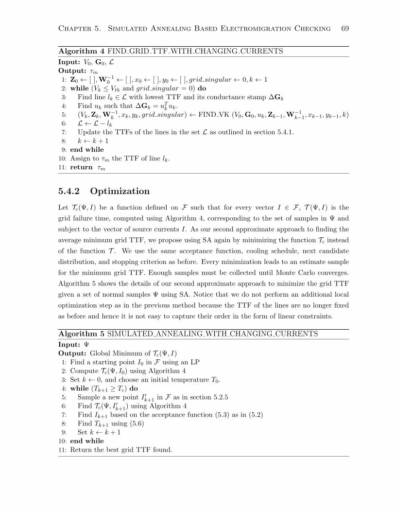
Chapter 5. Simulated Annealing Based Electromigration Checking 69
Algorithm 4 FIND GRID TTF WITH CHANGING CURRENTS
Input: V0, G0, LOutput: τm1: Z0 ← [ ],W−1
0 ← [ ], x0 ← [ ], y0 ← [ ], grid singular ← 0, k ← 12: while (Vk ≤ Vth and grid singular = 0) do3: Find line lk ∈ L with lowest TTF and its conductance stamp ∆Gk
4: Find uk such that ∆Gk = uTk uk.5: (Vk,Zk,W
−1k , xk, yk, grid singular) ← FIND VK (V0,G0, uk,Zk−1,W
−1k−1, xk−1, yk−1, k)
6: L ← L− lk7: Update the TTFs of the lines in the set L as outlined in section 5.4.1.8: k ← k + 19: end while
10: Assign to τm the TTF of line lk.11: return τm
5.4.2 Optimization
Let Tc(Ψ, I) be a function defined on F such that for every vector I ∈ F , T (Ψ, I) is the
grid failure time, computed using Algorithm 4, corresponding to the set of samples in Ψ and
subject to the vector of source currents I. As our second approximate approach to finding the
average minimum grid TTF, we propose using SA again by minimizing the function Tc insteadof the function T . We use the same acceptance function, cooling schedule, next candidate
distribution, and stopping criterion as before. Every minimization leads to an estimate sample
for the minimum grid TTF. Enough samples must be collected until Monte Carlo converges.
Algorithm 5 shows the details of our second approximate approach to minimize the grid TTF
given a set of normal samples Ψ using SA. Notice that we do not perform an additional local
optimization step as in the previous method because the TTF of the lines are no longer fixed
as before and hence it is not easy to capture their order in the form of linear constraints.
Algorithm 5 SIMULATED ANNEALING WITH CHANGING CURRENTS
Input: ΨOutput: Global Minimum of Tc(Ψ, I)1: Find a starting point I0 in F using an LP2: Compute Tc(Ψ, I0) using Algorithm 43: Set k ← 0, and choose an initial temperature T0.4: while (Tk+1 ≥ Tǫ) do5: Sample a new point I ′k+1 in F as in section 5.2.56: Find Tc(Ψ, I ′k+1) using Algorithm 47: Find Ik+1 based on the acceptance function (5.3) as in (5.2)8: Find Tk+1 using (5.6)9: Set k ← k + 1
10: end while
11: Return the best grid TTF found.

Chapter 5. Simulated Annealing Based Electromigration Checking 70
Table 5.1: Speed and accuracy comparison between the first Simulated Annealing basedmethod and the exact solution of chapter 4
Power Grid Exact Solution Simulated Annealing
ErrorName Nodes
Avg Min CPU Avg Min CPUTTF (yrs) Time TTF (yrs) Time
G1 141 7.50 3.21 min 7.39 2.12 min -1.47%G2 177 9.11 5.94 min 9.54 2.13 min 4.72%G3 237 10.38 25.10 min 9.91 2.44 min -4.53%G4 392 8.01 49.24 min 7.93 2.69 min -1.00%G5 586 9.79 4.42 h 10.05 2.58 min 2.66%
5.5 Optimization with Selective Updates
When estimating the EM statistics for step currents, the most computationally expensive steps
are updating the voltage drops and updating the TTFs after the failure of each line. In this
section, we describe a new approach for grid TTF estimation based on locality. The idea is
fully explained in [37] and emerges from observing that not all the nodes are equally impacted
when a line in the grid fails. In fact, only the nodes located in the immediate neighborhood of
the failing line are significantly impacted. This locality can be exploited to update the TTFs
of only a selection of the grid lines in order to speed-up the TTF estimation process at the cost
of some loss in accuracy.
Let N = {1, 2, . . . , n} denotes the set of all the nodes in the power grid. Also, let∂V[k]
∂Rdenotes the change in the voltage drop of node k with respect to the failure of interconnect R.
Define the set NR as follows:
NR =
{
k ∈ N :∂V[k]
∂R> δv
}
(5.20)
where δv is a user defined threshold. Finding NR can be done by checking which nodes in the
grid presented a change in their voltage drop larger than δv after the failure of R. The proposed
algorithm updates only the TTFs of the lines connected to the nodes in NR. A smaller value of
δv improves the accuracy of the estimated TTF at the cost of reduction in speed, and vice-versa.
As before, let Tl(Ψ, I) be a function defined on F such that for every vector I ∈ F , Tl(Ψ, I)is the grid failure time computed using Algorithm 4 but modified as to perform a selective TTF
update as explained above, corresponding to the set of samples in Ψ, and subject to the vector
of source currents I. As our third approximate approach to finding the average minimum grid
TTF, we use SA by minimizing the function Tl. Algorithm 6 shows the details of the proposed
approach. No additional local optimization is done here as well for the same reasons explained
in the previous section.

Chapter 5. Simulated Annealing Based Electromigration Checking 71
Algorithm 6 SIMULATED ANNEALING WITH SELECTIVE UPDATES
Input: ΨOutput: Global Minimum of Tc(Ψ, I)1: Find a starting point I0 in F using an LP2: Compute Tc(Ψ, I0) using Algorithm 43: Set k ← 0, and choose an initial temperature T0.4: while (Tk+1 ≥ Tǫ) do5: Sample a new point I ′k+1 in F as in section 5.2.56: Find Tc(Ψ, I ′k+1) using Algorithm 4 but modified as to perform a selective TTF update
as explained in section 5.57: Find Ik+1 based on the acceptance function (5.3) as in (5.2)8: Find Tk+1 using (5.6)9: Set k ← k + 1
10: end while
11: Return the best grid TTF found.
Table 5.2: Comparison of power grid average minimum TTF and CPU time for thethree Simulated Annealing based methods
Power SA with SA with SA with
Grid Local Opt Changing Currents Locality
Name NodesAvg.
CPU TimeAvg.
CPU TimeAvg.
CPU TimeMin TTF Min TTF Min TTF
G6 9K 15.14 yrs 17.4 min 15.05 yrs 9.6 min 15.26 yrs 8.0 minG7 19K 14.20 yrs 66.0 min 13.37 yrs 57.6 min 14.13 yrs 36.8 minG8 33K 12.19 yrs 2.3 hrs 12.18 yrs 2.5 hrs 12.18 yrs 1.5 hrsG9 51K 12.67 yrs 4.8 hrs 14.10 yrs 4.0 hrs 14.19 yrs 2.9 hrsG10 73K 12.48 yrs 7.2 hrs 13.89 yrs 6.6 hrs 13.98 yrs 3.9 hrsG11 132K 12.70 yrs 21.0 hrs 14.46 yrs 22.1 hrs 14.59 yrs 15.0 hrs
5.6 Experimental Results
Algorithms 3, 4, 5, and 6 have been implemented in C++. To solve the required linear programs
in algorithm 3, we again used the Mosek optimization package [29]. We use SPAI [30] as well to
compute the sparse inverse of G0. We carried out experiments on a set of randomly-generated
power grids, using a 2.6 GHz Linux machine with 24 GB of RAM. The grids are generated
based on user specifications, including grid dimensions, metal layers, pitch and width per layer,
and C4 and current source distribution. Moreover, all experiments were performed on grids
with up to ten global constraints (on groups of current sources). The parameters of the grids
are consistent with 1.1V 65nm CMOS technology. Notice that the first five grids (G1-G5) are
the same grids used in chapter 4. As for the EM model employed, we use similar parameters as
in the previous chapters: an activation energy of 0.9eV , a current exponent η = 1, a nominal
temperature Tm = 373K, a critical Blech product β = 3000A/cm, and a standard deviation

Chapter 5. Simulated Annealing Based Electromigration Checking 72
σln = 0.3. To asses the quality of our results, we computed the average worst-case grid TTF
using the SA with local optimization approach together with the required CPU time for every
grid. Table 5.1 shows the speed and accuracy of the simulated annealing approach by comparing
the obtained averages with the results of the exact approach of chapter 4. we can see that the
error is always less than ±5% while the run time is much less for the SA approach. The exact
approach required solving several ILPs and for that reason, the required CPU time is much
larger than that of the first SA based method. The observed accuracy for the small grids shows
that SA is able to explore the feasible space relatively well while reaching points very close to
the exact global optimum.
Table 5.2 shows the average minimum grid TTF obtained using the three Simulated Anneal-
ing based methods proposed for larger grids (G6-G11). As observed, the first method generally
generates a lower average minimum grid TTF than the other two methods because it includes
an additional local optimization step. The runtime of the second method is comparable to the
first because the TTF estimation in the second method requires updating the TTF of all the
lines in the grid every time a line fails, which is expensive. This problem is solved in the third
method where we see that the average minimum TTF obtained is very close to that of the
second method, while the run time is, on average, 1.5X better. The number of Monte Carlo
iterations that were required for convergence were between 30 and 40 for all the test grids.
Figure 5.3 shows the CPU time of all three methods versus the number of nodes in the grid.
Complexity analysis shows that the first two methods have around O(n1.6) empirical complexity
while the third have around O(n1.4) empirical complexity. Even though the first two methods
use different TTF estimators, the runtime for both methods is similar, and the reason is that
the second method uses a more expensive TTF estimator (the one developed in [37]) but does
not have the extra local optimization step. The average minimum TTF obtained are shown
in figure 5.4, where we can that the results of the second and third method almost overlap.
To better show the effectiveness of Simulated Annealing in finding the worst-case grid TTF,
figure 5.5 shows the progress of SA for all three methods for a particular Monte Carlo iteration
(33K nodes grid). We can see that SA is able to reduce the TTF estimated from around 21
years to 12 years. The local optimizer is able to provide a further reduction of 1 year (this
reduction always seems to be between 0.5 and 3 years for all the grids). In addition, the figure
shows that there is in fact a large separation between the TTF of the grid at different points
in space, i.e. the TTF of the grid is highly sensitive to the change in currents. This basically
means that it is not enough to compute the TTF of the grid at an arbitrary feasible point:
computing the minimum is necessary.
Lastly, and to check how sensitive SA is to the random seed used to travel the feasible
space, we minimized the TTF of grid G6 (using the optimization method of section 5.5) 50
times while keeping the same TTF samples for the grid lines and while changing the random
seed that controls how the next candidate points are being chosen. We obtained 50 different
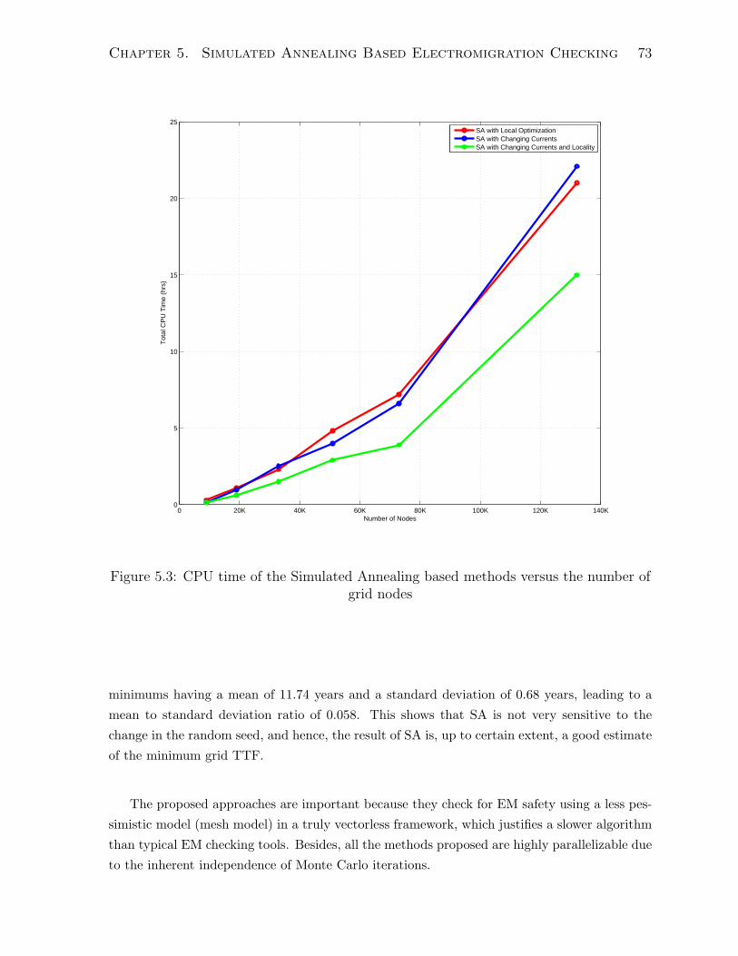
Chapter 5. Simulated Annealing Based Electromigration Checking 73
0 20K 40K 60K 80K 100K 120K 140K0
5
10
15
20
25
Number of Nodes
Tot
al C
PU
Tim
e (h
rs)
SA with Local OptimizationSA with Changing CurrentsSA with Changing Currents and Locality
Figure 5.3: CPU time of the Simulated Annealing based methods versus the number ofgrid nodes
minimums having a mean of 11.74 years and a standard deviation of 0.68 years, leading to a
mean to standard deviation ratio of 0.058. This shows that SA is not very sensitive to the
change in the random seed, and hence, the result of SA is, up to certain extent, a good estimate
of the minimum grid TTF.
The proposed approaches are important because they check for EM safety using a less pes-
simistic model (mesh model) in a truly vectorless framework, which justifies a slower algorithm
than typical EM checking tools. Besides, all the methods proposed are highly parallelizable due
to the inherent independence of Monte Carlo iterations.

Chapter 5. Simulated Annealing Based Electromigration Checking 74
0 20K 40K 60K 80K 100K 120K 140K0
2
4
6
8
10
12
14
16
18
20
Number of Nodes
Est
imat
ed A
vera
ge M
inim
um T
TF
(yr
s)
SA with Local OptimizationSA with Changing CurrentsSA with Changing Currents and Locality
Figure 5.4: Average minimum TTF estimated for the three Simulated Annealing basedmethods versus the number of grid nodes
5.7 Conclusion
We described three early vectorless approaches for power grid electromigration checking under
a constraint-based framework. The approaches employ the well known Simulated Annealing al-
gorithm. We show the accuracy of the methods as compared to the exact approach of chapter 4,
and show that the methods are very scalable as the complexity is slightly super linear.
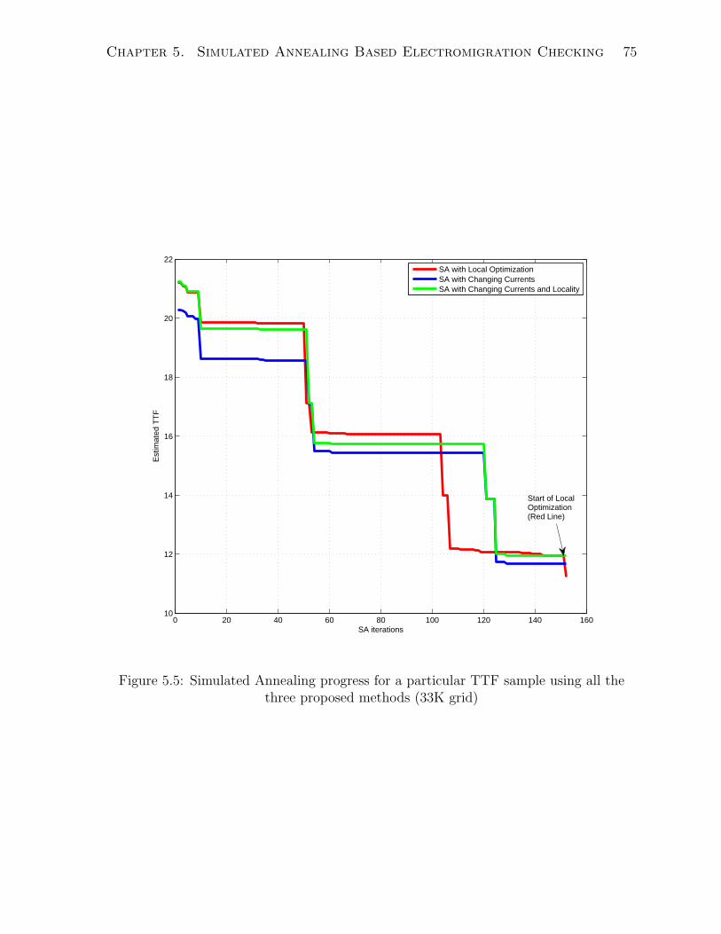
Chapter 5. Simulated Annealing Based Electromigration Checking 75
0 20 40 60 80 100 120 140 16010
12
14
16
18
20
22
SA iterations
Est
imat
ed T
TF
SA with Local OptimizationSA with Changing CurrentsSA with Changing Currents and Locality
Start of LocalOptimization(Red Line)
Figure 5.5: Simulated Annealing progress for a particular TTF sample using all thethree proposed methods (33K grid)

Chapter 6
Conclusion and Future Work
The latest trends toward low power and high performance semiconductor manufacturing has
emphasized the need for a robust design of the power delivery network. Every node in the
power grid must behave as a reliable source of supply voltage and must behave as such for a
certain number of years before failing. Timing violations and logic failures are bound to happen
when large voltage drops occur at grid nodes.
Under the effect of electromigration, metal line resistance increases as a line approaches
failure and starts to deform due to void creation. This affects the distribution of power among
grid nodes, and in most cases, leads to large voltage fluctuations. Accordingly, power grid
electromigration checking involves computing the mean time-to-failure of the power grid. Such
a metric gives the designer an idea about the robustness of the grid and whether it needs to be
redesigned or not.
Existing electromigration checking techniques and commercial tools assume the grid to be
a series system. As a result, the predicted EM stress is much worse than it actually is because
the grid is deemed to fail when any of its lines fail. This is leading to minimal margins between
the predicted EM stress and the EM design rules, making it very hard to sign-off chip designs
using traditional EM checking approaches. Therefore, there is a need to reconsider the existing
tools and to look with suspicion at the pessimism built into traditional EM checking methods.
Another critical aspect in EM checking, that which was the other focus of this thesis, is
the imprecise characterization of circuit currents. To capture this uncertainty, we built on the
framework of currents constraints as well as the constraints on the activity of different power
modes in every block. Verifying the power grids becomes a question of finding the average
worst-case time-to-failure of the power grid over all the possible chip workload scenarios. The
benefit of such a systematic framework is that it helps the user to manage design uncertainties
especially early in the design flow.
In chapter 3, we developed a new power grid MTF estimation technique to capture the
inherent redundancy in the grid. The method was verified using vector-based simulation where
76

Chapter 6. Conclusion and Future Work 77
we have shown that the MTF estimated is around 2-2.5X greater than the MTF predicted by
SEB. Besides, the method was shown to be runtime-efficient, scalable, and easily parallelizable.
In chapter 4, we extended the approach to the vectorless case, where an exact average worst-
case TTF of the grid was computed over all the possible chip workload scenarios using a set of
linear and mixed integer optimization problems. An important drawback of the exact approach
is that its runtime is too prohibitive for it to be scalable or useful except for small grids or
small islands in large grids. For that, chapter 5 introduces three more methods that are based
on the well known Simulated Annealing algorithm. The approaches are based on different TTF
estimation engines and were shown to be fairly accurate and relatively scalable. Collectively,
all the techniques presented can fill real and diverse design needs.
The research presented in this thesis seems to have raised many new questions with the
introduction of the mesh model. One might ask about the applicability of the model in modern
power grids where the lifetime of individual metal lines is governed by more complicated prob-
abilistic models than Black’s model. In addition, the approach must be extended to consider
better resistance evolution models for the failing lines. The infinite resistance was a simplifying
assumption which led to conservative yet possibly inaccurate results. On the other hand, a
Monte Carlo approach will always be relatively expensive and hence, one might want to look
into a direct approach for computing the MTF of the grid without the need for sampling. This
would also help the vectorless part of the work as it would make the Simulated Annealing based
algorithms much faster. Finally, it might be viable to explore existing model reduction schemes
which might allow hierarchical and incremental electromigration checking.

Bibliography
[1] J. Kitchin, “Statistical electromigration budgeting for reliable design and verification in a
300-MHz microprocessor,” in Symposium on VLSI Circuits Digest, 1995, pp. 115–116.
[2] M. Locatelli, Handbook of Global Optimization. Kluwer Academic Publishers, 2002, vol. 2,
ch. Simulated Annealing Algorithms for Continuous Global Optimization, pp. 179–229.
[3] J. R. Black, “Electromigration, a brief survey and some recent results,” IEEE transactions
on Electronic Devices, 1969.
[4] J. W. McPherson, Reliability Physics and Engineering. Springer, 2010.
[5] I. A. Blech, “Electromigration in thin aluminium on titanium nitride,” Journal of Applied
Physics, vol. 47, no. 4, pp. 1203–1208, 1976.
[6] A. Christou and M. Peckerar, Electromigration and Electronic Device Degradation. John
Wiley and Sons, 1994.
[7] G. Yoh and F. N. Najm, “A statistical model for electromigration failures,” in International
Symposium on Quality Electronic Design, San Jose, CA, Mar. 2000.
[8] B. Geden, “Unerstand and Avoid Electromigration (EM) & IR-drop in Custom IP Blocks,”
Synopsys, Tech. Rep., November 2011.
[9] J. R. Lloyd and J. Kitchin, “The electromigration failure distribution: The fine-line case,”
Journal of Applied Physics, February 1991.
[10] E. A. Amerasekera and F. N. Najm, Failure Mechanisms in Semiconductor Devices, 2nd ed.
John Wiley and Sons, 1997.
[11] D. Frost and K. F. Poole, “A method for predicting VLSI-device reliability using series
models for failure mechanisms,” IEEE Transactions on Reliability, vol. R-36, pp. 234–242,
1987.
[12] R. Ahmadi and F. N. Najm, “Timing analysis in presence of power supply and ground
voltage variations,” in IEEE/ACM International Conference on Computer-Aided Design,
San Jose, CA, November 2003.
78

Bibliography 79
[13] J. Warnock, “Circuit design challenges at the 14nm technology node,” in ACM/IEEE 47th
Design Automation Conference (DAC-2011), San Diego, CA, Jul. 5-9 2011.
[14] F. N. Najm, Circuit Simulation. John Wiley and Sons, 2010.
[15] S. Boyd and L. Vandenberghe, Convex Optimization. Cambridge University Press, 2004.
[16] G. Marsaglia and W. W. Tsang, “A fast, easily implemented method for sampling from
decreasing or symmetric unimodal density functions,” SIAM Journal of Scientific and
Statistical Computing, vol. 5, pp. 349–359, 1984.
[17] ——, “The ziggurat method for generating random variables,” Journal of Statistical Soft-
ware, vol. 5, 2000.
[18] ——, “Generating a variable from the tail of a normal distribution,” Technometrics, vol. 6,
pp. 101–102, 1964.
[19] J. E. Freund, I. R. Miller, and R. Johnson, Probability and Statistics for Engineers, 6th ed.
Prentice-Hall, 2010.
[20] F. N. Najm, “Statistical estimation of the signal probability in VLSI circuits,” University
of Illinois at Urbana-Champaign, Coordinated Science Laboratory, Tech. Rep. UILU-ENG-
93-2211, April 1993.
[21] L. Doyen, E. Petitprez, P. Waltz, X. Federspiel, L. Arnaud, and Y. Wouters, “Extensive
analysis of resistance evolution due to electromigration induced degradation,” Journal of
Applied Physics, 2008.
[22] L. Arnaud, P. Lamontagne, F. Bana, Y. L. Friec, , and P. Waltz, “Study of electromi-
gration void nucleation time in cu interconnects with doping elements,” Microelectronic
Engineering, April 2012.
[23] B. Li, T. D. Sullivan, T. C. Lee, and D. Badami, “Reliability challenges for copper inter-
connects,” Microelectronics Reliability, March 2004.
[24] S. Chatterjee, M. Fawaz, and F. N. Najm, “Redundancy-aware electromigration check-
ing for mesh power grids,” in IEEE/ACM International Conference On Computer-Aided
Design, San Jose, CA, Nov. 2013.
[25] N. J. Higham, Functions of Matrices: theory and computation, 1st ed. SIAM, 2008.
[26] Y. Tian and Y. Takane, “Schur complements and banachiewicz-schur forms,” Electronic
Journal of Linear Algebra, vol. 13, pp. 405–418, Dec 2005.

Bibliography 80
[27] D. Kouroussis and F. N. Najm, “A static patter-independent technique for power grid
voltage integrity verification,” in ACM/IEEE Design Automation Conference, Anaheim,
CA, June 2003.
[28] H. Kellere, U. Pferschy, and D. Pisinger, Knapsack Problems. Springer, 2004.
[29] The MOSEK optimization software. [Online]. Available: http://www.mosek.com
[30] N. H. Abdul Ghani and F. N. Najm, “Fast vectorless power grid verification using an ap-
proximate inverse technique,” in ACM/IEEE Design Automation Conference, San Fran-
sisco, CA, Jul. 26-31 2009.
[31] S. Kirkpatric, C. Gelatt, and M. Vecchi, “Optimization by simulated annealing,” Science,
vol. 220, pp. 671–680, 1983.
[32] V. Cerny, “Thermodynamical approach to the travelling salesman problem: An efficient
simulation algorithm,” Journal of Optimization Theory and Applications, vol. 45, pp. 41–
51, 1985.
[33] N. Metropolis, A. Rosentbluth, M. Rosentbluth, and A. Teller, “Equation of state calcu-
lations by fast computer machines,” J. Chem. Phys., 1953.
[34] I. Bohachevsky, M. Johnson, and M. Stein, “Generalized simulated annealing for function
optimization,” Technometrics, vol. 28, pp. 895–901, 1986.
[35] H. Romeijn and R. Smith, “Simulated annealing for constrained global optimization,”
Journal of Global Optimization, vol. 5, pp. 101–126, 1994.
[36] H. Romeijn, Z. Zabinski, D. Graesser, and S. Neogi, “New reflection generator for simu-
lated annealing in mixed-integer/continuous global optimization,” Journal of Optimization
Theory and Applications, vol. 101, pp. 403–427, 1999.
[37] S. Chatterjee, “Redundancy aware electromigration checking for mesh power grids,” Mas-
ter’s thesis, University of Toronto, August 2013.