ELECTROMAGNETICFIELDFROMAHORIZONTAL ... spherical conducting or electrically earth coated with a...

Progress In Electromagnetics Research, PIER 54, 221–244, 2005

ELECTROMAGNETIC FIELD FROM A HORIZONTALELECTRIC DIPOLE IN THE SPHERICALELECTRICALLY EARTH COATED WITH N-LAYEREDDIELECTRICS

K. Li †

The Electromagnetics Academy at Zhejiang UniversityZhejiang UniversityZijingang Campus, Hangzhou, Zhejiang, 310058, P. R. China

Y.-L. Lu

School of Electrical and Electronic EngineeringNanyang Technological UniversitySingapore 639798

Abstract—In this paper, the electromagnetic field in air froma radiating horizontal electric dipole located in the homogeneousisotropic spherical electrically earth coated with N -layered dielectricsis investigated anew. The starting point is based on the formulas forthe electromagnetic fields in air from vertical electric and magneticdipoles situated in air above the surface of the earth coated with N -layered dielectrics. The complete explicit formulas are derived for theelectromagnetic fields in the earth due to vertical electric and magneticdipoles located in air. By using reciprocity theorem, the formulas arereadily obtained for the six components of the electromagnetic field inair radiated by a horizontal electric dipole located in the earth.

1 Introduction

2 The EM Field in the Earth due to a Vertical ElectricDipole Situated in Air

3 The EM Field in the Earth due to a Vertical MagneticDipole Situated in Air

† Also with the School of Electrical and Electronic Engineering, Nanyang TechnologicalUniversity, Singapore 639798

222 Li and Lu

4 The EM Field in Air of a Horizontal Electric DipoleLocated in the Earth

5 Computations and Analysis

6 Conclusions

References

1. INTRODUCTION

The problem of the electromagnetic (EM) field from a dipole sourcelocated on or near the surface of the spherical earth has been a subjectof interest for many years. The early classic harmonic-series solutionfor a dipole in the presence of a homogeneous sphere was begun byWatson [1]. The subsequent further developments were made by otherpioneers [2–11], such as Van del Pol, Fock, Bremmer, Norton, and Wait.Despite the remarkable progress that had already been made on thisproblem, some aspects of it remained in the dark. The problem wasrecently reexamined by Houdzoumis [12, 13] and Margetis [14]. Theexact formulas are obtained for the complete EM field on the surfaceof the spherical earth when vertical and horizontal electric dipoles arelocated on that surface.

When the spherical earth is covered with layered dielectrics,the derivations of the EM field radiated by a dipole source are ingeneral much more complicated. In [15–17], the complete explicitformulas have been derived for the EM field of a dipole source overthe spherical conducting or electrically earth coated with a dielectriclayer. Furthermore, the general case of the EM field radiated by adipole source near the surface of the spherical earth coated with N -layered dielectrics has been treated in [18].

In what follows, we will attempt to determine the EM field from ahorizontal electric dipole located in the spherical electrically earth. Thestarting point is based on the formulas for the EM fields in air due tovertical electric and magnetic dipoles situated in air above the surfaceof the earth coated with N -layered dielectrics addressed in [18]. Byusing boundary conditions, the formulas of the EM fields in the earthdue to vertical electric and magnetic dipoles located in air are derivedreadily. Based on the above results, using the reciprocity theorem, theformulas are obtained for the six components of the EM field froma horizontal electric dipole located in the earth. To illustrate theapplications of the formulas obtained, computations are carried outwhen the layered dielectrics are composed of successive 2 sphericallybounded layers, each with the thickness l/2.

Progress In Electromagnetics Research, PIER 54, 2005 223

2. THE EM FIELD IN THE EARTH DUE TO AVERTICAL ELECTRIC DIPOLE SITUATED IN AIR

x

y0

Region 0:

Region n:

Region n+1:

1k

0k

nk

1nk

),,(rVED

Region 1:

z

ar

'1lar

'nlar

'1nlar

=

=

=

=

−

−

−

−

θ φ

+

...

Figure 1. The vertical electric dipole at the height zs in air abovethe surface of the spherical earth coated with N -layered dielectrics:l′j = l1 + · · · + lj , j = 1, 2, ..., n.

In this section we will start with the formulas for the EM fieldin air due to a vertical electric dipole over the surface of the sphericalearth coated with N -layered dielectrics addressed in [18]. Assumingthat dipole is represented by the current density zIdlδ(x)δ(y)δ(z − b),where b = zs + a, and zs > 0 denotes the height of the dipole abovethe surface of the spherical earth coated with N -layered dielectrics, therelevant geometry is illustrated in Fig. 1. The general case of sphericallayering is that the layered dielectrics above the earth are composed ofsuccessive N spherically bounded layers, each with arbitrary thicknesslj , j = 1, 2, ..., n. The center of the sphere is the origin of a coordinate

224 Li and Lu

system (r, θ, φ). The air (Region 0, r ≥ a) is characterized by thepermeability µ0, uniform permittivity ε0, and conductivity σ0 = 0.The N -layered dielectrics with the uniform thickness l consists of Nspherical layers, e.g., l = l1 + l2 + · · · + ln. The dielectric in Regionj (a − l

′j ≤ r ≤ a − l

′j−1) is characterized by the permeability µ0,

relative permittivity εrj , and conductivity σj . The earth (Region n+1,r ≤ a− l

′n) is the dielectric medium characterized by the permeability

µ0, relative permittivity εr(n+1), and conductivity σn+1. With use ofa harmonic time factor e−iωt, the wave numbers of those regions are

k0 = ω√µ0ε0,

kj = ω√µ0 (ε0εrj + iσj/ω), j = 1, 2, ..., n,

kn+1 = ω

√µ0

(ε0εr(n+1) + iσn+1/ω

). (1)

The complete formulas for the components E(0)r , E(0)

θ , and H(0)φ of the

EM field in the air due to a vertical electric dipole at (a + zs, 0, 0),which is defined as the electric-type field, have been obtained in [18].They are

E(0)r

E(0)θ

H(0)φ

=iIdl · ηλa

· ei(kaθ+π

4)

√θ sin θ

·√πx

×

∑s

Fs(zs) · Fs(zr)ts − q2

· eitsx

∑s

iFs(zs) ·∂Fs(z)k0∂z

|z=zr

(ts − q2)

[1 +

ts2

(2k0a

)2/3] · eitsx

∑s

Fs(zs) · Fs(zr)/η0

(ts − q2)

[1 +

ts2

(2k0a

)2/3] · eitsx

(2)

Here, θ = d/a, d is the great-circle distance between the dipole sourceand the observer, and a is the earth radius. x = (k0a/2)1/3 θ is anormalized range parameter, and ts(s = 1, 2, ...) are the roots of themode equation.

W′2(t) − qW2(t) = 0, (3)


where

q = i1η0

(k0a

2

) 13

· Z0(a). (4)

The surface impedance, Z0(a), at the boundary between Regions 0 and1 has been obtained in [18]. It is

Z0(r)∣∣∣∣r=a

= −ωµ0γ1

k21

· tanh

{iγ1l1 + tanh−1

[γ2 · k2

1

γ1 · k22

· tanh[iγ2l2

+ tanh−1[γ3 · k2

2

γ2 · k23

· tanh[iγ3l3 + · · · + tanh−1

[γn · k2

n−1

γn−1 · k2n

· tanh[iγnln + tanh−1

(kn · �g

γn

) ]]· · ·

]]]]}. (5)

The “height-gain” function Fs(z) is defined by

Fs(z) =W2(ts − y)W2(ts)

, (6)

where

y =[2ν(ν + 1)

a3

]1/3

z ≈(

2k0a

)1/3

k0z. (7)

Here, W2 is the Airy function of the second kind. zr denotes the heightof the observer above the surface of the earth coated with N-layereddielectrics. It is noted that zs and zr are somewhat less than the range,d, while the latter is less than the earth radius, a.

It is seen that, in Region j (j = 1, 2, ..., n), the non-zerocomponents E(j)

r , E(j)θ , and H

(j)φ of the EM field can be expressed in

terms of the potential function, Uj , which is the solution of the scalarHelmholtz equation

(∇2 + k2j )Uj = 0, (8)

In spherical coordinates, because of symmetry, a solution for Uj iswritten in the form of

Uj =1rRj(r)Φ(θ). (9)

It is well known that the azimuthal field variations can be expressedin terms of the Legendre functions of the first kind Pν(cos(π− θ)) and

226 Li and Lu

their derivatives [15–18]. The radial field variations are determined bythe following differential equation.

d2Rj(r)dr2

+ k2j

[1 − ν(ν + 1)

k2j r

2

]Rj(r) = 0. (10)

In Region j (j = 1, 2, ..., n), a − l′j ≤ r ≤ a − l

′j−1, l

′j � a, we take

r ≈ a. Taking into account ν(ν+1) ≈ k20a

2, the solution of (10), whichhas been addressed specifically in [18], can be written as follows:

Rj(r) = Bjeiγj ·[r−(a−l

′j)] + Cje

−iγj ·[r−(a−l′j)]. (11)

where γj =√k2

j − k20, j = 1, 2, ..., n. The surface impedance, Zj(r), at

any point in Region j for the EM field of electric type can be expressedas follows:

Zj(r) =E

(j)θ

H(j)φ

= −ωµ0γj

k2j

· Bjeiγj ·[r−(a−l

′j)] − Cje

−iγj ·[r−(a−l′j)]

Bneiγn·[r−(a−l

′j)] + Cje

−iγj ·[r−(a−l′j)]

= −ωµ0γj

k2j

· tanh[ln

(Bj

Cj

) 12

+ iγj [r − (a− l′j)]

].

(12)

Taking into account the impedance boundary conditionZ1(r)|r=a = Z0(r)|r=a at r = a, which is between Regions 0 and 1,it is easily obtained

�1E =B1

C1= exp

{2 tanh−1

[γ2 · k2

1

γ1 · k22

· tanh[iγ2l2 + tanh−1

[γ3 · k2

2

γ2 · k23

· tanh[iγ3l3 + · · · + tanh−1

[γn · k2

n−1

γn−1 · k2n

× tanh[iγnln + tanh−1

(kn · �g

γn

) ]]· · ·

]]]]},

(13)

With the boundary condition Z2(r)|r=a−l1= Z1(r)|r=a−l1

at r = a−l1,we get

�2E =B2

C2= exp

{2 tanh−1

[γ3 · k2

2

γ2 · k23

· tanh[iγ3l3 + tanh−1

[γ4 · k2

3

γ3 · k24


× tanh[iγ3l3 + · · · + tanh−1

[γn · k2

n−1

γn−1 · k2n

· tanh[iγnln

+ tanh−1(kn · �g

γn

) ]]· · ·

]]]]}. (14)

With the boundary condition at r = a− l′j (l′j = l1 + l2 + ...+ lj), whichis between Regions j and j + 1, we obtain

�jE =Bj

Cj= exp

{2 tanh−1

[γj+1 · k2

j

γj · k2j+1

· tanh[iγjlj + tanh−1

[γj+1 · k2

j

γj · k2j+1

· tanh[iγj+1lj+1+· · ·+tanh−1

[γn · k2

n−1

γn−1 · k2n


(kn · �g

γn

) ]]· · ·

]]]]}. (15)

With the boundary condition at r = a− l′n (l′n = l1 + l2 + ...+ ln = l),we find

�nE =Bn

Cn= exp

[2 tanh−1

(kn · �g

γn

) ]. (16)

When the observer lies on the boundary between Regions 0 and1, zr = 0, Fs(0) = 1, ∂Fs(zr)/(k0∂z)|zr=0 = −iZ0/η0. The completeformulas for the components Er, Eθ, and Hφ of the EM field in Region1 (a − l1 < r < a) due to a vertical electric dipole at (a + zs, 0, 0) inRegion 0 (r > a) can be derived readily.

E(1)r

E(1)θ

H(1)φ

=iIdl · ηλa

· ei(k0aθ+π

4)

√θ sin θ

·√πx

×

k20

k21

· �(1)1E ·

∑s

Fs(zs)ts − q2

· eitsx

�(2)1E · ∑

s

Fs(zs) · Z0(a)/η0

(ts − q2)

[1 +

ts2

(2k0a

)2/3] · eitsx

�(3)1E ·

∑s

Fs(zs)/η0

(ts − q2)

[1 +

ts2

(2k0a

)2/3] · eitsx

, (17)

228 Li and Lu

where

�(1)

1E

�(2)1E

�(3)1E

=

�1E · eiγ1[r−(a−l1)] + e−iγ1[r−(a−l1)]

�1E · eiγ1l1 + e−iγ1l1

�1E · eiγ1[r−(a−l1)] − e−iγ1[r−(a−l1)]

�1E · eiγ1l1 − e−iγ1l1

�1E · eiγ1[r−(a−l1)] + e−iγ1[r−(a−l1)]


. (18)

On applying the boundary conditions at r = a − l1, r = a − l2,...,r = a−ln, we can write the complete formulas for the components E(n)

r ,E

(n)θ , andH(n)

φ of the EM field at the boundary r = a−l (l = l1+...+ln)radiated by a vertical electric dipole at (a + zs, 0, 0) in air (Region 0,r > a).E

(n)r

E(n)θ

H(n)φ

r=a−l

=iIdl · ηλa

· ei(k0aθ+π

4)

√θ sin θ

·√πx

×

k20

k2n

· �(1)nE ·

∑s

Fs(zs)ts − q2

· eitsx

�(2)nE ·

∑s

Fs(zs) · Z0(a)/η0

(ts − q2)

[1 +

ts2

(2k0a

)2/3] · eitsx

�(3)nE ·

∑s

Fs(zs)/η0

(ts − q2)

[1 +

ts2

(2k0a

)2/3] · eitsx

,

(19)

where

�(1)

nE

�(2)nE

�(3)nE

= ei(γ1l1+γ2l2+...+γnln) ·

n∏j=1

�jE + 1�jE · ei2γj lj + 1

n∏j=1

�jE − 1�jE · ei2γj lj − 1

n∏j=1

�jE + 1�jE · ei2γj lj + 1

. (20)

Consequently, we obtain the following expressions for the EM field of


electric type in Region n+1.E

(n+1)r

E(n+1)θ

H(n+1)φ

r=a−l−dr

=iIdl · ηλa

· ei(k0aθ+kn+1dr+π

4)

√θ sin θ

·√πx

×

k20

k2n+1

· �(1)nE ·

∑s

Fs(zs)ts − q2

· eitsx

�(2)nE ·

∑s

Fs(zs) · Z0(a)/η0

(ts − q2)

[1 +

ts2

(2k0a

)2/3] · eitsx

�(3)nE ·

∑s

Fs(zs)/η0

(ts − q2)

[1 +

ts2

(2k0a

)2/3] · eitsx

.

(21)

3. THE EM FIELD IN THE EARTH DUE TO AVERTICAL MAGNETIC DIPOLE SITUATED IN AIR

In this section we will start with the formulas for the EM field inair due to a vertical magnetic dipole over the surface of the sphericalearth coated with N -layered dielectrics. When the dipole source at(a+zs, 0, 0) is replaced by the vertical magnetic dipole with its momentM = Ida, and da is the area of the loop, the complete formulas forthe components E(0)

φ , H(0)r , and H

(0)θ of the EM field over the surface

of the spherical earth coated with the N -layered dielectrics, which isdefined as the magnetic-type field, have been derived in [18]. They are

E

(0)φ

H(0)r

H(0)θ

=ωµ0Ida

λa

ei(k0aθ+π4)

√θ sin θ

·√πx

∑s

Gs(zs)Gs(zr)ts − (qh)2

eit′sx

1η0

∑s

Gs(zs)Gs(zr)ts − (qh)2

eit′sx

i

η0

∑s

Gs(zs)∂Gs(z)k0∂z

|z=zr

ts − (qh)2eit′sx

,

(22)

230 Li and Lu

where

Gs(z) =W2(t

′s − y)

W2(t′s)

, (23)

is a “height-gain” function, and W2(t′s) is the Airy function of the

second kind. Here, t′s(s = 1, 2, ...) are the roots of the following mode

equation

W′2(t

′) − qhW2(t

′) = 0, (24)

where

qh =iωµ0

k0·(k0a

2

) 13

· Y0(a). (25)

The surface admittance, Y0(a), at r = a is expressed as follows:

Y0(r)|r=a = − γ1

ωµ0tanh

{iγ1l1 + tanh−1

[γ2

γ1· tanh

[iγ2l2

+ tanh−1[γ3

γ2· tanh

[iγ3l3 + · · · + tanh−1

[γn

γn−1


(− kn

γn · �g

)]]· · ·

]]]]}.

(26)

In Region j, the components E(0)φ , H(0)

r , and H(0)θ of the EM field

can be expressed in terms of a potential function, Vj , which is thesolution of the following scalar Helmholtz equation

(∇2 + k2j )Vj = 0. (27)

Similarly, the azimuthal field variations are expressed in terms of theLegendre functions of the first kind Pν(cos(π−θ)) and their derivatives,and the radial field variations are written as

R′j(r) = B

′je

iγj ·[r−(a−l′j)] + C

′je

−iγj ·[r−(a−l′j)]. (28)

Then, the quantity Yj(r) of the surface admittance in Region j for theEM field of magnetic type can be arrived at the following expressions.

Yj(r) =H

(j)θ

E(j)φ

= − γj

ωµ0·B′

jeiγj [r−(a−l

′j)] − C ′

ne−iγj [r−(a−l

′j)]

B′je

iγj [r−(a−l′j)] + C ′

je−iγj [r−(a−l

′j)]

= tanh

{ln

(B′

j

C ′j

)1/2

+ iγj [r − (a− l′j)]

}. (29)


Taking into account the impedance boundary condition Y1(r)|r=a =Y0(r)|r=a at r = a, it is easily obtained.

�1M =B′

1

C ′1

= exp

{2 tanh−1

[γ2

γ1· tanh

[iγ2l2 + tanh−1

[γ3

γ2

× tanh[iγ3l3 + · · · + tanh−1

[γn

γn−1· tanh

[iγnln

+ tanh−1(− kn

γn · �g

)]]· · ·

]]]]}, (30)

With the boundary condition Y2(r)|r=a−l′ = Y1(r)|r=a−l′ at r = a− l′1,we get

�2M =B

′2

C′2

= exp

{2 tanh−1

[γ3

γ2· tanh

[iγ3l3 + tanh−1

[γ4

γ3

× tanh[iγ3l3 + · · · + tanh−1

[γn

γn−1· tanh

[iγnln

+ tanh−1(− kn

γn · �g

)]]· · ·

]]]]}, (31)

With the boundary condition at r = a− l′j (l′j = l1 + l2 + ...+ lj), weobtain

�jM =B′

j

C ′j

= exp

{2 tanh−1

[γj+1

γj· tanh

[iγjlj + tanh−1

[γj+1

γj

× tanh[iγj+1lj+1 + · · · + tanh−1

[γn

γn−1· tanh

[iγnln

+ tanh−1(− kn

γn · �g

)]]· · ·

]]]]}, (32)

With the boundary condition at r = a − l, (l = l1 + l2 + ... + ln), wefind

�nM =B′

n

C ′n

= exp

[2 tanh−1

(− kn

γn · �g

)]. (33)

When the observer lies on the boundary between Regions 0 and1, zr = 0, Gs(0) = 1, ∂Gs(zr)/(k0∂z)|zr=0 = −iη0Y0(a), the complete

formulas for the components E(1)φ , H(1)

r , and H(1)θ of the EM field

232 Li and Lu

in Region 1 (a − l1 < r < a) due to a vertical magnetic dipole at(a+ zs, 0, 0) in Region 0 (r > a) are obtained as follows:

E(1)φ

H(1)r

H(1)θ

=iωµ0Ida

λa· e

i(k0aθ+π4)

√θ sin θ

·√πx

×

�(1)1M ·

∑s

Gs(zs)t′s − (qh)2

· eit′sx

�(2)1M ·

∑s

Gs(zs)/η0

t′s − (qh)2· eit′sx

�(3)1M ·

∑s

Gs(zs) · Y0(a)/η0


, (34)

where

�(1)

1M

�(2)1M

�(3)1M

=

�1M · eiγ1[r−(a−l1)] + e−iγ1[r−(a−l1)]

�1M · eiγ1l1 + e−iγ1l1

�1M · eiγ1[r−(a−l1)] + e−iγ1[r−(a−l1)]


�1M · eiγ1[r−(a−l1)] − e−iγ1[r−(a−l1)]

�1M · eiγ1l1 − e−iγ1l1

. (35)

With the boundary conditions at r = a− l′1, r = a− l′2, ..., r = a− l′n,we arrive at the following formulas for the components E(n)

r , E(n)θ , and

H(n)φ of the EM field at the r = a− l (l = l1 + ...+ ln).

E(n)φ

H(n)r

H(n)θ

r=a−l

=ωµ0Ida

λa· e

i(k0aθ+π4)

√θ sin θ

·√πx

×

�(1)nM ·

∑s


· eit′sx

�(2)nM ·

∑s


· eit′sx

�(3)nM ·

∑s

Gs(zs)Y0(a)/η0


, (36)


where

�(1)

nM

�(2)nM

�(3)nM

= ei(γ1l1+γ2l2+···+γnln) ·

n∏j=1

�jM + 1�jM · ei2γj lj + 1

n∏j=1

�jM + 1�jM · ei2γj lj + 1

n∏j=1

�jM − 1�jM · ei2γj lj − 1

. (37)

Then, it follows the complete formulas for the EM field in Regionn+ 1.

E(n+1)φ

H(n+1)r

H(n+1)θ

r=a−l−dr

=ωµ0Ida

λa· e

i(k0aθ+kn+1dr+π4)

√θ sin θ

·√πx

×

�(1)nM ·

∑s

Gs(zs)ts − (qh)2

· eit′sx

�(2)nM ·

∑s

Gs(zs)/η0

t′s − (qh)2· eitsx

�(3)nM ·

∑s

Gs(zs)Y0(a)/η0

ts − (qh)2· eit′sx

. (38)

4. THE EM FIELD IN AIR OF A HORIZONTALELECTRIC DIPOLE LOCATED IN THE EARTH

In this section, we attempt to formulate the formulas of the EM fieldin air due to a horizontal electric dipole, Ids he Idshe, which is locatedat the depth ds of the earth, as illustrated in Fig. 2. From the aboveexpressions of the EM fields in the earth (Region n+ 1) from verticalelectric and magnetic dipoles in air (Region 0), by using reciprocitytheorem, it is fairly straightforward to arrive the expressions of thevertical electric field E

he(0)r and the vertical magnetic field H

he(0)r in

air when a horizontal electric dipole is located in the earth.

Ehe(0)r = − iηIds

he

λa· e

i(k0aθ+kn+1ds+π4)

√θ sin θ

·√πx · cosφ

234 Li and Lu

x

y0

Region 0:

Region n:

Region n+1:

1k

0k

nk

1nk

),,(r

HED

Region 1:

z

ar

'1lar

'nlar

'1nlar

=

=

=

=

−

−

−

−

θ φ

+

Figure 2. The horizontal electric dipole at the depth ds in thespherical earth coated with N -layered dielectrics: l

′j = l1 + · · · + lj ,

j = 1, 2, ..., n.

×∑s

�(2)nE · Z0(a)/η0 · Fs(zr)

(ts − q2)

[1 +

ts2

(2k0a

)2/3] · eitsx, (39)

Hhe(0)r = − iIds

he

λa· e

i(k0aθ+kn+1ds+π4)

√θ sin θ

·√πx · sinφ

×∑s

�(1)nM ·Gs(zr)t′s − (qh)2

· eit′sx. (40)

Here, φ is the orientation angle between the dipole source and theobserver, and the horizontal dipole is located at (a − l − ds, 0, 0).In spherical coordinates, from Maxwell’s equations, the rest four


components Ehe(0)θ , Ehe(0)

φ , Hhe(0)θ , and H

he(0)φ can be expressed in

terms of Ehe(0)r and H

he(0)r .(

∂2

∂r2+ k2

)(rHhe(0)

φ ) = iωε0∂E

he(0)r

∂θ+

1sin θ

∂2Hhe(0)r

∂r∂φ, (41)(

∂2

∂r2+ k2

)(rEhe(0)

θ ) =∂2E

he(0)r

∂r∂θ+iωµ0

sin θ∂H

he(0)r

∂φ, (42)(

∂2

∂r2+ k2

)(rHhe(0)

θ ) = − iωε0sin θ

∂Ehe(0)r

∂φ+∂2H

he(0)r

∂r∂θ, (43)(

∂2

∂r2+ k2

)(rEhe(0)

φ ) =1

sin θ∂2E

he(0)r

∂r∂φ− iωµ0

∂Hhe(0)r

∂θ. (44)

From (41), we get

ν(ν + 1)r

(Hhe(0)φ ) = iωε0

∂Ehe(0)r

∂θ+

1sin θ

∂2Hhe(0)r

∂r∂φ. (45)

Taking into account the relation ν(ν + 1)/r ≈ k20a, as a result of some

straightforward operations we obtain the following expression for thecomponent Hhe(0)

φ .

Hhe(0)φ = − iIds

he

λa· e

i(k0aθ+kn+1ds+π4)

√θ sin θ

·√πx · cosφ

×[∑

s

�(2)nE · Z0(a)/η0 · Fs(zr)

ts − q2· eitsx +

1k0a sin θ

×∑s

�(1)nM · ∂Gs(z)

k0∂z|z=zr

t′s − (qh)2· eit

′sx

. (46)

Similarly, we obtain

Hhe(0)θ =

Idshe

λa· e

i(k0aθ+kn+1ds+π4)

√θ sin θ

·√πx · sinφ

×

1k0a sin θ

∑s

�(2)nE · Z0(a)/η0 · Fs(zr)

(ts − q2)

[1 +

ts2

(2k0a

)2/3] · eitsx

236 Li and Lu

−∑s

�(1)nM · ∂Gs(z)

k0∂z|z=zr

t′s − (qh)2· eit

′sx

, (47)

Ehe(0)θ =

ηIdshe

λa· e

i(k0aθ+kn+1ds+π4)

√θ sin θ

·√πx · cosφ

×

−∑s

�(2)nE · Z0(a)/η0 ·

∂Fs(z)k0∂z

|z=zr

ts − q2· eitsx

+1

k0a sin θ·∑s


· eit′sx

], (48)

Ehe(0)φ =

iηIdshe

λa· e

i(k0aθ+kn+1ds+π4)

√θ sin θ

·√πx · sinφ

×

i

k0a sin θ·∑s

�(2)nE · Z0(a)/η0 ·

∂Fs(z)k0∂z

|z=zr

(ts − q2)

[1 +

ts2

(2k0a

)2/3] · eitsx

+∑s


· eit′sx

], (49)

where the superscript he designates that the EM field is radiated by ahorizontal electric dipole. From the results obtained, it is seen that theEM field consists of the electric-type and magnetic-type terms when ahorizontal electric dipole is located in the earth coated with N-layereddielectrics.

5. COMPUTATIONS AND ANALYSIS

To illustrate the complete formulas for the EM field in N -layeredspherical regions from a dipole source, the computations are carriedout when the layered dielectrics are composed of a succession of 2spherically bounded layers, each with the thickness l/2. Assumingthat l = 100 m, the radius of the earth is a = 6370 km, Region 1(a− l/2 < r < a) is characterized by the relative permittivity εr1 = 10and conductivity σ1 = 10−5 S/m, Region 2 (a − l < r < a − l/2) is


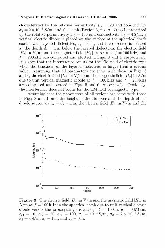
characterized by the relative permittivity εr2 = 20 and conductivityσ2 = 2×10−5 S/m, and the earth (Region 3, r < a− l) is characterizedby the relative permittivity εr3 = 100 and conductivity σ3 = 4 S/m, avertical electric dipole is placed on the surface of the spherical earthcoated with layered dielectrics, zs = 0 m, and the observer is locatedat the depth dr = 1 m below the layered dielectrics, the electric field|Er| in V/m and the magnetic field |Hφ| in A/m at f = 100 kHz, andf = 200 kHz are computed and plotted in Figs. 3 and 4, respectively.It is seen that the interference occurs for the EM field of electric typewhen the thickness of the layered dielectrics is larger than a certainvalue. Assuming that all parameters are same with those in Figs. 3and 4, the electric field |Eφ| in V/m and the magnetic field |Hr| in A/mdue to unit vertical magnetic dipole at f = 100 kHz and f = 200 kHzare computed and plotted in Figs. 5 and 6, respectively. Obviously,the interference does not occur for the EM field of magnetic type.

Assuming that the parameters of all regions are same with thosein Figs. 3 and 4, and the height of the observer and the depth of thedipole source are zr = ds = 1 m, the electric field |Er| in V/m and the

0 50 100 150 200 250 30010

9

108

107

106

105

ρ (km)

Mag

nitu

des

| Er | in V/m

| Hφ | in A/m

−

−

−

−

−

Figure 3. The electric field |Er| in V/m and the magnetic field |Hφ| inA/m at f = 100 kHz in the spherical earth due to unit vertical electricdipole versus the propagating distance ρ; l = 100 m, a = 6370 km,εr1 = 10, εr2 = 20, εr3 = 100, σ1 = 10−5 S/m, σ2 = 2 × 10−5 S/m,σ3 = 4 S/m, dr = 1 m, and zs = 0 m.

238 Li and Lu

0 50 100 150 200 250 30010 11

10 10

10 9

10 8

10 7

10 6

10 5

ρ (km)

Mag

nitu

des

| Er | in V/m

| Hφ | in A/m

−

−

−

−

−

−

−

Figure 4. The electric field |Er| in V/m and the magnetic field |Hφ| inA/m at f = 200 kHz in the spherical earth due to unit vertical electricdipole versus the propagating distance ρ; l = 100 m, a = 6370 km,εr1 = 10, εr2 = 20, εr3 = 100, σ1 = 10−5 S/m, σ2 = 2 × 10−5 S/m,σ3 = 4 S/m, dr = 1 m, and zs = 0 m.

0 50 100 150 200 250 30010

17

1016

1015

1014

1013

1012

1011

1010

ρ (km)

Mag

nitu

des

| Eφ | in V/m

| Hr | in A/m

−

−

−

−

−

−

−

−

Figure 5. The electric field |Eφ| in V/m and the magnetic field |Hr| inA/m in the spherical earth at f = 100 kHz due to unit vertical magneticdipole versus the propagating distance ρ; l = 100 m, a = 6370 km,εr1 = 10, εr2 = 20, εr3 = 100, σ1 = 10−5 S/m, σ2 = 2 × 10−5 S/m,σ3 = 4 S/m, dr = 1 m, and zs = 0 m.


0 50 100 150 200 250 30010

16

1015

1014

1013

1012

1011

1010

109

ρ (km)

Mag

nitu

des

| Eφ | in V/m

| Hr | in A/m

−

−

−

−

−

−

−

−

Figure 6. The electric field |Eφ| in V/m and the magnetic field |Hr| inA/m in the earth at f = 200 kHz due to unit vertical magnetic dipoleversus the propagating distance ρ; l = 100 m, a = 6370 km, εr1 = 10,εr2 = 20, εr3 = 100, σ1 = 10−5 S/m, σ2 = 2 × 10−5 S/m, σ3 = 4 S/m,dr = 1 m, and zs = 0 m.

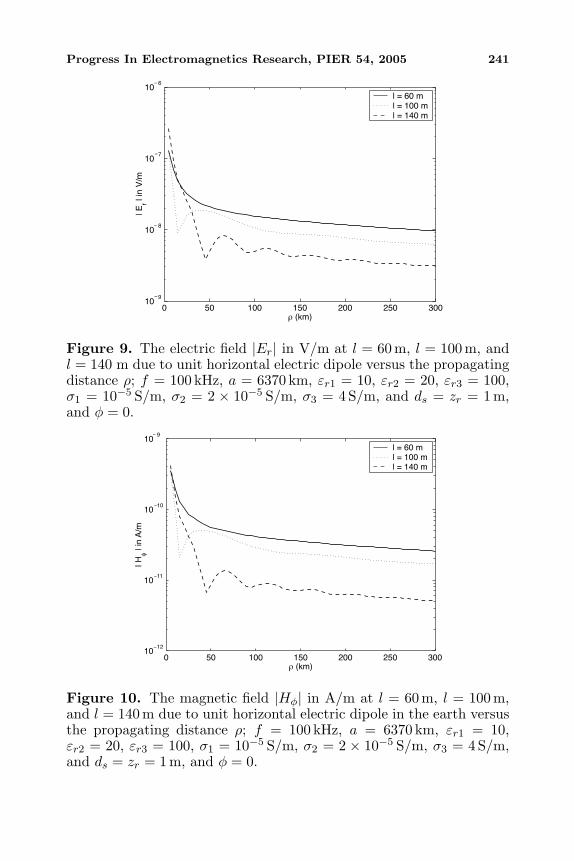
magnetic fields |Hφ| in A/m due to unit horizontal electric dipole atf = 100 kHz and f = 200 kHz are calculated and plotted in Figs. 7 and8, respectively. In order to demonstrate the influence of the thickness ofthe layered dielectrics, the electric fields |Er| in V/m and the magneticfields |Hφ| in A/m at l = 60 m, l = 100 m, and l = 140 m are shown inFigs. 9 and 10, respectively.

6. CONCLUSIONS

From the above derivations and computations, it is seen that theinterference occurs for the EM field radiated by horizontal or verticalelectric dipoles when the thickness of the layered dielectrics is largerthan a certain value and the interference does not occur for the EMfield radiated by vertical magnetic dipole. It has been demonstratedthat the excitation efficiency of horizontal or vertical electric dipolesis much higher than that of a vertical magnetic dipole. The formulasand computations for the EM field radiated by electrically horizontalantenna located in the earth or vertical antenna in air have usefulapplications in the communication to the observer in the air or in theasphalt- and cement-coated spherical earth at low frequencies.

240 Li and Lu

0 50 100 150 200 250 30010

10

109

108

107

106

ρ (km)

| Er |

in V

/m

f = 100 MHzf = 200 MHz

−

−

−

−

−

Figure 7. The electric field |Er| in V/m in the air at f = 100 kHzand f = 200 kHz due to unit horizontal electric dipole in the earthversus the propagating distance ρ; l = 100 m, a = 6370 km, εr1 = 10,εr2 = 20, εr3 = 100, σ1 = 10−5 S/m, σ2 = 2 × 10−5 S/m, σ3 = 4 S/m,and ds = zr = 1 m, and φ = 0.

0 50 100 150 200 250 30010

13

1012

1011

1010

109

108

ρ (km)

| Hφ |

in A

/m

f = 100 MHzf = 200 MHz

−

−

−

−

−

−

Figure 8. The magnetic field |Hφ| in A/m at f = 100 kHz and f =200 kHz due to unit horizontal electric dipole versus the propagatingdistance ρ; l = 100 m, a = 6370 km, εr1 = 10, εr2 = 20, εr3 = 100,σ1 = 10−5 S/m, σ2 = 2 × 10−5 S/m, σ3 = 4 S/m, and ds = zr = 1 m,and φ = 0.


0 50 100 150 200 250 30010

9

108

107

106

ρ (km)

| Er |

in V

/m

l = 60 ml = 100 ml = 140 m

−

−

−

−

Figure 9. The electric field |Er| in V/m at l = 60 m, l = 100 m, andl = 140 m due to unit horizontal electric dipole versus the propagatingdistance ρ; f = 100 kHz, a = 6370 km, εr1 = 10, εr2 = 20, εr3 = 100,σ1 = 10−5 S/m, σ2 = 2 × 10−5 S/m, σ3 = 4 S/m, and ds = zr = 1 m,and φ = 0.

0 50 100 150 200 250 30010

12

1011

1010

109

ρ (km)

| Hφ |

in A

/m

l = 60 ml = 100 ml = 140 m

−

−

−

−

Figure 10. The magnetic field |Hφ| in A/m at l = 60 m, l = 100 m,and l = 140 m due to unit horizontal electric dipole in the earth versusthe propagating distance ρ; f = 100 kHz, a = 6370 km, εr1 = 10,εr2 = 20, εr3 = 100, σ1 = 10−5 S/m, σ2 = 2 × 10−5 S/m, σ3 = 4 S/m,and ds = zr = 1 m, and φ = 0.

242 Li and Lu

REFERENCES

1. Watson, G. N., “The diffraction of radio waves by the earth,”Proc. the Royal Society, Vol. A95, 83–99, 1918.

2. Van der Pol, B. and H. Bremmer, “The propagation of radio wavesover a finitely conducting spherical earth,” Phil. Mag., Vol. 25,817–834, 1938; Further note on above, Vol. 27, 261–275, 1939.

3. Fock, V. A., Electromagnetic Diffraction and PropagationProblems, 191–212, Pergamon Press, Ltd., Oxford, 1965.

4. Bremmer, H., Terrestrial Radio Waves, Elsevier, New York, 1949.5. Bremmer, H., “Applications of operational calculus to ground-

wave propagation, particularly for long waves,” IRE Trans.Antennas Porpag., Vol. AP-6, 267–274, 1958.

6. North, K. A., “The calculations of ground-wave field intensity overa finitely conducting spherical earth,” Proc. IRE, Vol. 29, 623–639,1941.

7. Wait, J. R., “Radiation and propagation from a vertical antennaover a spherical earth,” Journal of Research of National Bureauof Standards, Vol. 56, 237–244, 1956.

8. Wait, J. R., “The electromagnetic field of a horizontal dipole inthe presence of a conducting half-space,” Can. J. Phys., Vol. 39,1017–1027, 1961.

9. Wait, J. R. and D. A. Hill, “Excitation of the HF surface wave byvertical and horizontal antennas,” Radio Sci., Vol. 14, 767–780,1979.

10. Hill, D. A. and J. R. Wait, “Ground wave attenuation function fora spherical earth with arbitrary surface impedance,” Radio Sci.,Vol. 15, No. 3, 637–643, 1980.

11. Wait, J. R., “The ancient and modern history of EM ground-wavepropagation,” IEEE Antennas and Propagat. Mag., Vol. 40, No. 5,7–24, 1998.

12. Houdzoumis, V. A., “Vertical electric dipole radiation over asphere: character of the waves that propagate through thesphere,” J. Appl. Phys., Vol. 86, 3939–3942, 1999.

13. Houdzoumis, V. A., “Two modes of wave propagation manifestedin vertical electric dipole radiation over a sphere,” Radio Sci.,Vol. 35, No. 1, 19–29, 2000.

14. Margetis, D., “Radiation of horizontal electric dipole on largedielectric sphere,” J. Math. Phys., Vol. 43, 3162–3201, 2002.

15. Pan, W. Y. and H. Q. Zhang, “Electromagnetic field of avertical electric dipole on the surface of a dielectric layer


overlay a global conductor,” Radio Sci., Vol. 38, No. 3, 1061,10.1029/2002RS002689, 2003.

16. Li, K. and S.-O. Park, “Electromagnetic field in the air generatedby a horizontal electric dipole located in the spherical electricallyearth coated with a dielectric layer,” J. Electromagn. WavesApplicat., Vol. 17, No. 10, 1399–1417, 2003.

17. Li, K., S.-O. Park, and H.-Q. Zhang, “Electromagnetic field inthe presence of a three-layered spherical region,” Progress InElectromagnetics Research, J. A. Kong (ed.), Vol. 45, 103–121,EMW Publishing, Cambridge, Boston, 2004.

18. Li, K., S.-O. Park, and H.-Q. Zhang, “The electromagnetic fieldover the spherical earth coated with N-layered dielectric,” RadioSci., Vol. 39, RS2008, doi:10.1029/2002RS002771, 2004.

19. Gradshteyn, I. S. and I. M. Ryzhik, Table of Integrals, Series, andProducts, Academic Press, New York, 1980.

Kai Li was born in Xiao County, Anhui, China on February 10,1968. He received his B.Sc. degree in Physics from Fuyang NormalCollege, Anhui, China, in 1990, M.Sc. degree in Radio Physics fromXidian University, Xi’an, Shaanxi, China, in 1994, and Ph.D. degreein Astrophysics from Shaanxi Astronomical Observatory, the ChineseAcademy of Sciences, Shaanxi, China, in 1998, respectively. FromAugust 1990 to December 2000, he was on the faculty of ChinaResearch Institute Radiowave Propagation (CRIRP). From January2001 to December 2002, he was with Information and CommunicationsUniversity (ICU), Taejon, South Korea as a Postdoctoral fellow. FromJanuary 2003 to January 2005, he was with the School of Electricaland Electronic Engineering, Nanyang Technological University (NTU),Singapore as a research fellow. Since January 2005, he was withthe Electromagnetics Academy (TEA) at Zhejiang University (ZJU),Zijingang Campus, Zhejiang University, China, where he is currentlya full professor in TEA at ZJU. His research interests include classicelectromagnetic theory and radio wave propagation. Dr. Li is a seniormember of Chinese Institute of Electronics (CIE) and a member ofChinese Institute of Space Science (CISS).

Yilong Lu was born in Chengdu, China. He received the B.Eng.degree from Harbin Institute of Technology, China, in 1982, the M.Eng.degree from Tsinghua University, China, in 1984, and the Ph.D.degree in 1991 from University College of London, U.K., in 1991,all in electronic engineering. From 1984 to 1988, he was with theAntenna Division in University of Electronic Science and Technology

244 Li and Lu

of China, Chengdu, China. Since 1992, he has been with the Schoolof Electrical and Electronic Engineering, Nanyang TechnologicalUniversity, Singapore, where he is currently an Associate Professorin the Communication Engineering Division. His research interestsare computational electromagnetics, antennas, array signal processing,and evolutionary computation for engineering optimization.

ELECTROMAGNETICFIELDFROMAHORIZONTAL ... spherical conducting or electrically earth coated with a...

Documents

Transcript of ELECTROMAGNETICFIELDFROMAHORIZONTAL ... spherical conducting or electrically earth coated with a...