
ELECTROMAGNETIC THEORY EKT 241/4: ELECTROMAGNETIC THEORY PREPARED BY: NORDIANA MOHAMAD SAAID...
67
EKT 241/4: ELECTROMAGNETIC THEORY ELECTROMAGNETIC THEORY PREPARED BY: NORDIANA MOHAMAD SAAID [email protected] CHAPTER 5 – TRANSMISSION LINES U N I V E R S I T I M A L A Y S I A P E R L I S U N I V E R S I T I M A L A Y S I A P E R L I S
-
Upload
nicholas-booker -
Category
Documents
-
view
237 -
download
6
Transcript of ELECTROMAGNETIC THEORY EKT 241/4: ELECTROMAGNETIC THEORY PREPARED BY: NORDIANA MOHAMAD SAAID...

EKT 241/4: ELECTROMAGNETIC ELECTROMAGNETIC THEORYTHEORY
PREPARED BY: NORDIANA MOHAMAD [email protected]
CHAPTER 5 – TRANSMISSION LINES
UN
IVE
RS
ITI M
AL
AY
SIA
PE
RL
ISU
NIV
ER
SIT
I MA
LA
YS
IA P
ER
LIS

Chapter Outline
General ConsiderationsLumped-Element ModelTransmission-Line EquationsWave Propagation on a Transmission LineThe Lossless Transmission Line Input Impedance of the Lossless LineSpecial Cases of the Lossless LinePower Flow on a Lossless Transmission LineThe Smith Chart Impedance MatchingTransients on Transmission Lines

General Considerations
• Transmission line – a two-port network connecting a generator circuit to a load.

The role of wavelength
• The impact of a transmission line on the current and voltage in the circuit depends on the length of line, l and the frequency, f of the signal provided by generator.
• At low frequency, the impact is negligible• At high frequency, the impact is very significant

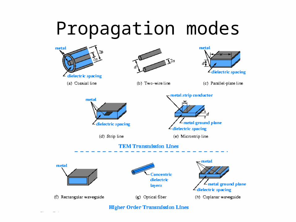
Propagation modes
• Transmission lines may be classified into two types:a) Transverse electromagnetic (TEM) transmission lines – waves propagating along these lines having electric and magnetic field that are entirely transverse to the direction of propagation b) Higher order transmission lines – waves propagating along these lines have at least one significant field component in the direction of propagation
Propagation modes

Lumped- element model

Lumped- element model
• A transmission line is represented by a parallel-wire configuration regardless of the specific shape of the line, i.e coaxial line, two-wire line or any TEM line.
• Lumped element circuit model consists of four basic elements called ‘the transmission line parameters’ : R’ , L’ , G’ , C’ .

Lumped- element model
• Lumped-element transmission line parameters:– R’ : combined resistance of both conductors
per unit length, in Ω/m– L’ : the combined inductance of both
conductors per unit length, in H/m– G’ : the conductance of the insulation medium
per unit length, in S/m– C’ : the capacitance of the two conductors per
unit length, in F/m

Lumped- element model
Note: µ, σ, ε pertain to the insulating material between conductors

Lumped- element model
• All TEM transmission lines share the following relation:
''CL
'
'
C
G
Note: µ, σ, ε pertain to the insulating material between conductors

Transmission line equations
• Complex propagation constant, γ
• α – the real part of γ - attenuation constant, unit: Np/m
• β – the imaginary part of γ - phase constant, unit: rad/m
j
CjG'LjR'
''

Transmission line equations
• The characteristic impedance of the line, Z0 :
• Phase velocity of propagating waves:
where f = frequency (Hz) λ = wavelength (m)
''
''0 CjG
LjRZ
fu p

Example 1
An air line is a transmission line for which air is the dielectric material present between the two conductors, which renders G’ = 0.
In addition, the conductors are made of a material with high conductivity so that R’ ≈0.
For an air line with characteristic impedance of 50Ω and phase constant of 20 rad/m at 700MHz, find the inductance per meter and the capacitance per meter of the line.

Solution to Example 1
• The following quantities are given:
• With R’ = G’ = 0,
• The ratio is given by
• We get L’ from Z0
Hz 107 MHz 700 rad/m, 20 ,50 80 fZ
'
'
'
' and ''''Im 0 C
L
Cj
LjZCLCjLj
pF/m 9.90501072
20'
80
Z
C
nH/m 227109.9050''' 1220 LCLZ

Lossless transmission line
• Lossless transmission line - Very small values of R’ and G’.
• We set R’=0 and G’=0, hence:
line) (lossless ''
line) (lossless 0
CL
line) (lossless '
'
0,G' and 0R' since
''
''
0
0
C
LZ
CjG
LjRZ
Lossless transmission line
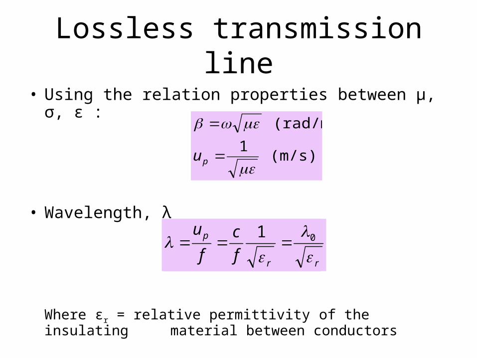
• Using the relation properties between μ, σ, ε :
• Wavelength, λ
Where εr = relative permittivity of the insulating material between conductors
(m/s) 1
(rad/m)
pu
rr
p
f
c
f
u
01
Voltage reflection coefficient
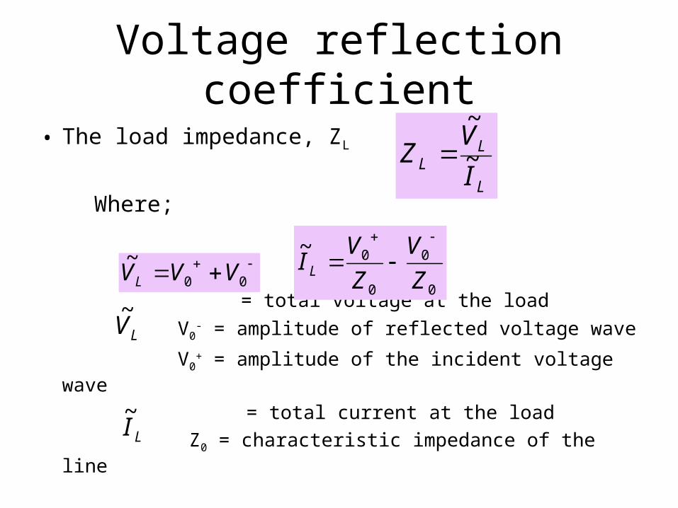
• The load impedance, ZL
Where;
= total voltage at the load
V0- = amplitude of reflected voltage wave
V0+ = amplitude of the incident voltage wave
= total current at the load
Z0 = characteristic impedance of the line
00
~VVVL
LV~
0
0
0
0~
Z
V
Z
VI L
LI~
L
LL
I
VZ ~
~

Voltage reflection coefficient
• Hence, load impedance, ZL:
• Solving in terms of V0- :
0
00
00 ZVV
VVZ L
00
00 V
ZZ
ZZV
L
L

Voltage reflection coefficient
• Voltage reflection coefficient, Γ – the ratio of the amplitude of the reflected voltage wave, V0
- to the amplitude of the incident voltage wave, V0
+ at the load.
• Hence,
less)(dimension 1
1
0
0
0
0
0
0
ZZ
ZZ
ZZ
ZZ
V
V
L
L
L
L

Voltage reflection coefficient
• Z0 for lossless line is a real number while ZL in general is a complex number. Hence,
Where |Γ| = magnitude of Γ
θr = phase angle of Γ
• A load is matched to the line if ZL = Z0 because there will be no reflection by the load (Γ = 0 and V0
−= 0.
rje

Voltage reflection coefficient
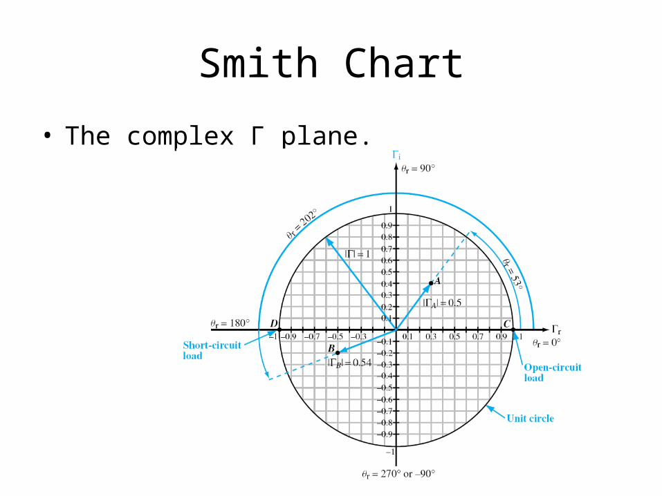
• When the load is an open circuit, (ZL=∞), Γ = 1 and V0
- = V0+.
• When the load is a short circuit (ZL=0), Γ = -1 and V0
- = V0+.

Example 2
• A 100-Ω transmission line is connected to a load consisting of a 50-Ω resistor in series with a 10pF capacitor. Find the reflection coefficient at the load for a 100-MHz signal.

Solution to Example 2
• The following quantities are given
• The load impedance is
• Voltage reflection coefficient is
Hz10MHz100 ,100 F,10 ,50 80
11LL fZCR
1595010102
150
/
118
LLL
jj
CjRZ
7.6076.0159.15.0
159.15.0
1/
1/
0L
0L
j
j
ZZ
ZZ

Standing Waves
• Interference of the reflected wave and the incident wave along a transmission line creates a standing wave.
• Constructive interference gives maximum value for standing wave pattern, while destructive interference gives minimum value.
• The repetition period is λ for incident and reflected wave individually.
• But, the repetition period for standing wave pattern is λ/2.

Standing Waves
• For a matched line, ZL = Z0, Γ = 0 and
= |V0+| for all values of z. zV
~

Standing Waves
• For a short-circuited load, (ZL=0), Γ = -1.

Standing Waves
• For an open-circuited load, (ZL=∞), Γ = 1.
The wave is shifted by λ/4 from short-circuit case.
Standing Waves
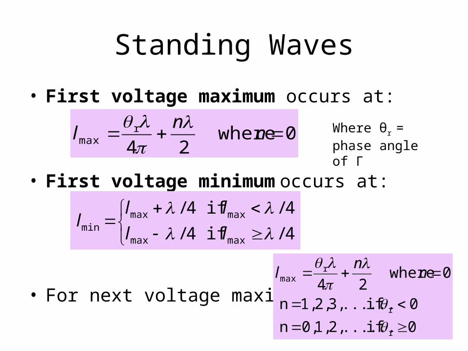
• First voltage maximum occurs at:
• First voltage minimum occurs at:
• For next voltage maximum:
0 where24
rmax n
nl
4/ if 4/
4/ if 4/
maxmax
maxmaxmin
ll
lll
0 if ...... 2, 1, 0, n
0 if ...... 3, 2, 1, n
0 where24
r
r
rmax
nn
l
Where θr = phase angle of Γ

Voltage standing wave ratio
• VSWR is the ratio of the maximum voltage amplitude to the minimum voltage amplitude:
• VSWR provides a measure of mismatch between the load and the transmission line.
• For a matched load with Γ = 0, VSWR = 1 and for a line with |Γ| - 1, VSWR = ∞.
less)(dimension 1
1~
~
min
max
V
VVSWR

Example 3
A 50- transmission line is terminated in a load with ZL = (100 + j50)Ω . Find the voltage reflection coefficient and the voltage standing-wave ratio (VSWR).

Solution to Example 3
• We have,
• VSWR is given by:
6.26
0L
0L 45.05050100
5050100
1/
1/ jej
j
ZZ
ZZ
6.245.01
45.01
1
1
VSWR
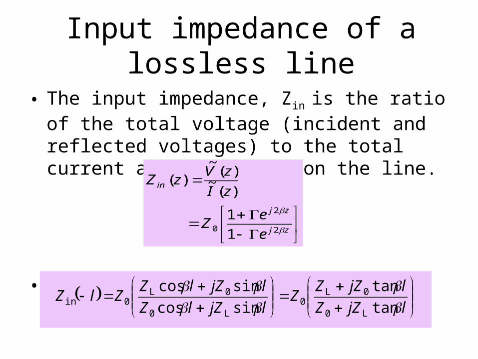
Input impedance of a lossless line
• The input impedance, Zin is the ratio of the total voltage (incident and reflected voltages) to the total current at any point z on the line.
• or
ljZZ
ljZZZ
ljZlZ
ljZlZZlZ
tan
tan
sincos
sincos
L0
0L0
L0
0L0in
zj
zj
in
e
eZ
zI
zVzZ
2
2
0 1
1
)(~
)(~
)(

Special cases of the lossless line
• For a line terminated in a short-circuit, ZL = 0:
• For a line terminated in an open circuit, ZL = ∞:
ljZlI
lVZ tan~
~
0
sc
scscin
ljZ
lI
lVZ cot~ 0
oc
ococin

Application of short-circuit and open-circuit measurements
• The measurements of short-circuit input impedance, and open-circuit input impedance, can be used to measure the characteristic impedance of the line:
• and
scinZ
ocinZ
ocin
scin ZZZo
ocin
scintan
Z
Zl
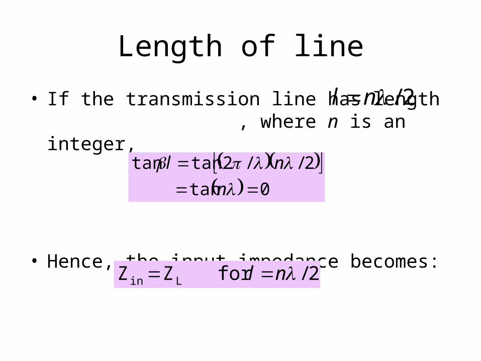
Length of line
• If the transmission line has length , where n is an integer,
• Hence, the input impedance becomes:
2/nl
0tan
2//2tantan
n
nl
2/for ZZ Lin nl
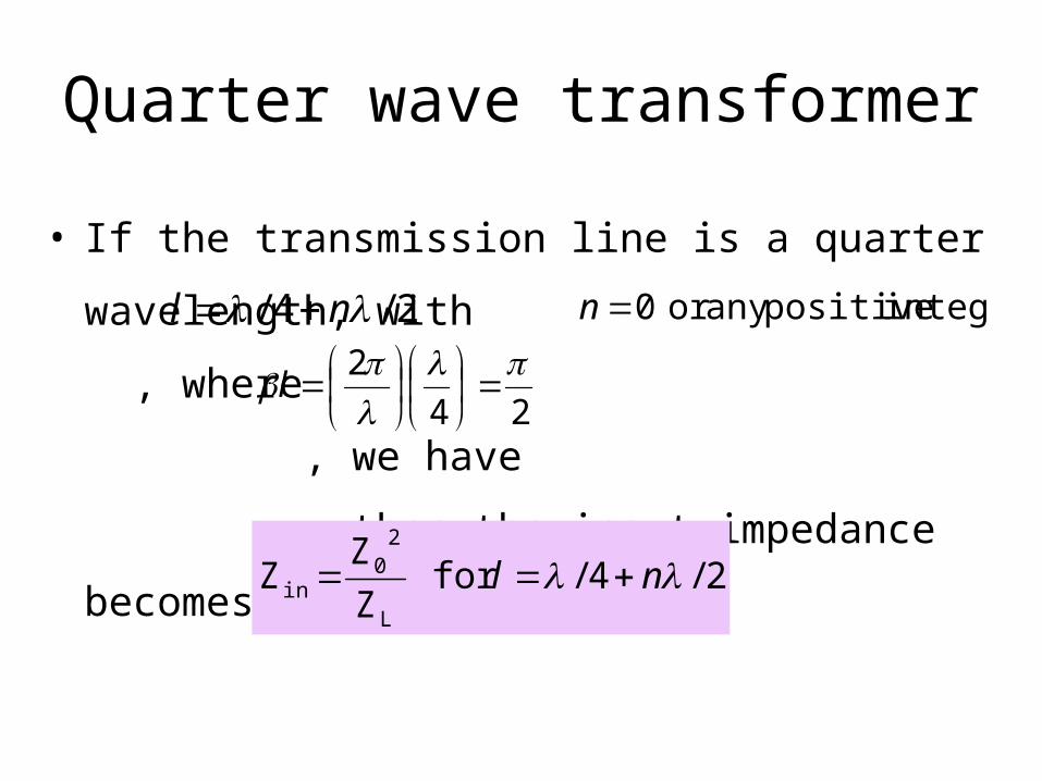
Quarter wave transformer
• If the transmission line is a quarter wavelength,
with ,
where , we have
, then the input impedance becomes:
2/4/ nl integer positiveany or 0n
24
2
l
2/4/for Z
ZZ
L
20
in nl

Example 4
A 50-Ω lossless transmission line is to be matched to a resistive load impedance with ZL=100Ω via a quarter-wave section as shown, thereby eliminating reflections along the feedline. Find the characteristic impedance of the quarter-wave transformer.

Solution to Example 4
• To eliminate reflections at terminal AA’, the input impedance Zin looking into the quarter-wave line should be equal to Z01 (the characteristic impedance of the feedline). Thus, Zin = 50Ω .
• Since the lines are lossless, all the incident power will end up getting transferred into the load ZL.
7.701005002
L
202
in
Z
Z
ZZ

Matched transmission line
• For a matched lossless transmission line, ZL=Z0:
1) The input impedance Zin=Z0 for all locations z on the line,
2) Γ =0, and
3) all the incident power is delivered to the load, regardless of the length of the line, l.

Power flow on a lossless transmission line
• Two ways to determine the average power of an incident wave and the reflected wave;– Time-domain approach– Phasor domain approach
• Average power for incident wave;
• Average power for reflected wave:
(W) 2 0
2
0iav Z
VP
iav
2
0
2
02rav 2
PZ
VP
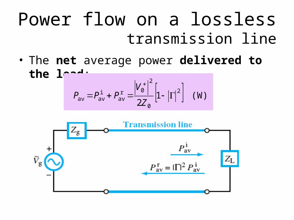
Power flow on a lossless transmission line
• The net average power delivered to the load:
(W) 12
2
0
2
0rav
iavav
Z
VPPP

Smith Chart
• Smith chart is used to analyze & design transmission line circuits.
• Impedances on Smith chart are represented by normalized value, zL for example:
• the normalized load impedance, zL is dimensionless.
0Z
Zz L
L

Smith Chart
• Reflection coefficient, Γ :
• Since , Γ becomes:
• Re-arrange in terms of zL:
• Normalized load admittance:
1/
1/
0
0
ZZ
ZZ
L
L
0Z
Zz L
L 1
1
L
L
z
z
LL jxrz
1
1L
1
11
LL z
y
Smith Chart
• The complex Γ plane.
Smith Chart
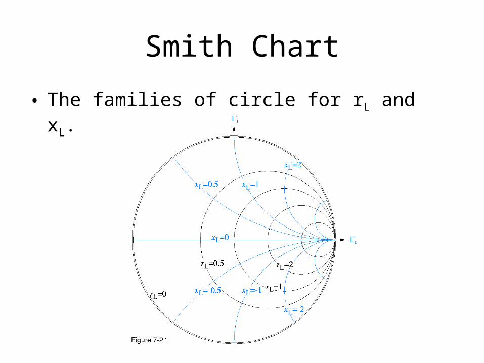
• The families of circle for rL and xL.

Smith Chart
• Plotting normalized impedance, zL = 2-j1

Input impedance
• The input impedance, Zin:
• Γ is the voltage reflection coefficient at the load.
• We shift the phase angle of Γ by 2βl, to get ΓL. This will zL to zin. The |Γ| is the same, but the phase is changed by 2βl.
• On the Smith chart, this means rotating in a clockwise direction (WTG).
lj
lj
in e
eZZ
2
2
0 1
1
Input impedance
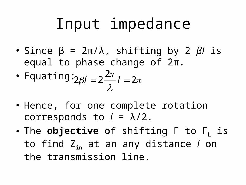
• Since β = 2π/λ, shifting by 2 βl is equal to phase change of 2π.
• Equating:
• Hence, for one complete rotation corresponds to l = λ/2.
• The objective of shifting Γ to ΓL is to find Zin at an any distance l on the transmission line.
2
222 ll

Example 5
• A 50-Ω transmission line is terminated with ZL=(100-j50)Ω. Find Zin at a distance l =0.1λ from the load.

Solution to Example 5
at B, zin = 0.6 –j0.66

VSWR, Voltage Maxima and Voltage Minima
VSWR, Voltage Maxima and Voltage Minima
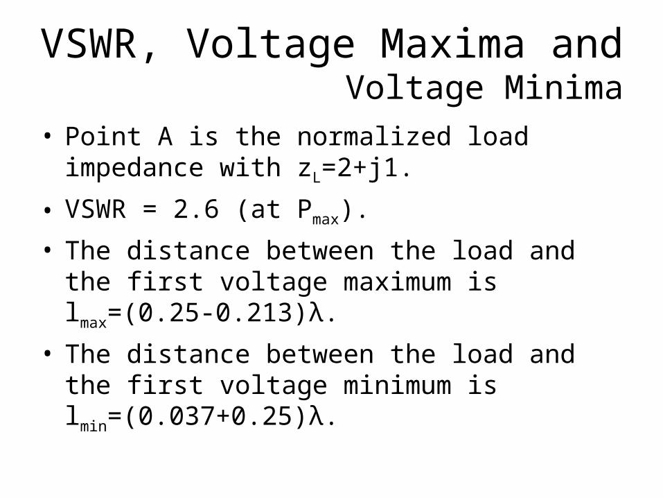
• Point A is the normalized load impedance with zL=2+j1.
• VSWR = 2.6 (at Pmax).
• The distance between the load and the first voltage maximum is lmax=(0.25-0.213)λ.
• The distance between the load and the first voltage minimum is lmin=(0.037+0.25)λ.
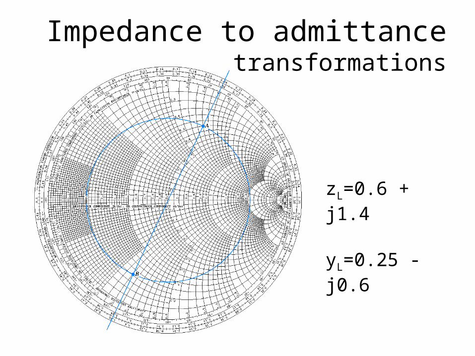
Impedance to admittance transformations
yL=0.25 - j0.6
zL=0.6 + j1.4

Example 6
• Given that the voltage standing-wave ratio, VSWR = 3. On a 50-Ω line, the first voltage minimum occurs at 5 cm from the load, and that the distance between successive minima is 20 cm, find the load impedance.

Solution to Example 6
• The distance between successive minima is equal to λ/2. Hence, λ = 40 cm.
• First voltage minimum (in wavelength unit) is at
on the WTL scale from point B.
• Intersect the line with constant SWR circle = 3.• The normalized load impedance at point C is:
• De-normalize (multiplying by Z0) to get ZL:
125.040
5min l
8.06.0L jz
40308.06.050L jjZ

Solution to Example 6
Impedance Matching
• Transmission line is matched to the load when Z0 = ZL.
• This is usually not possible since ZL is used to serve other application.
• Alternatively, we can place an impedance-matching network between load and transmission line.

Single- stub matching
• Matching network consists of two sections of transmission lines.
• First section of length d, while the second section of length l in paralllel with the first section, hence it is called stub.
• The second section is terminated with either short-circuit or open circuit.

Single- stub matching

Single- stub matching
• The distance d is chosen so as to transform the load admittance, YL=1/ZL into an admittance of the form Yd = Y0+jB when looking towards the load at MM’.
• The length l of the stub is chosen so that its input admittance, YS at MM’ is equal to –jB.
• Hence, the parallel sum of the two admittances at MM’ yields Y0, which is the characteristic admittance of the line.
Example 7
50-Ω transmission line is connected to an antenna with load impedance ZL = (25 − j50)Ω. Find the position and length of the short-circuited stub required to match the line.

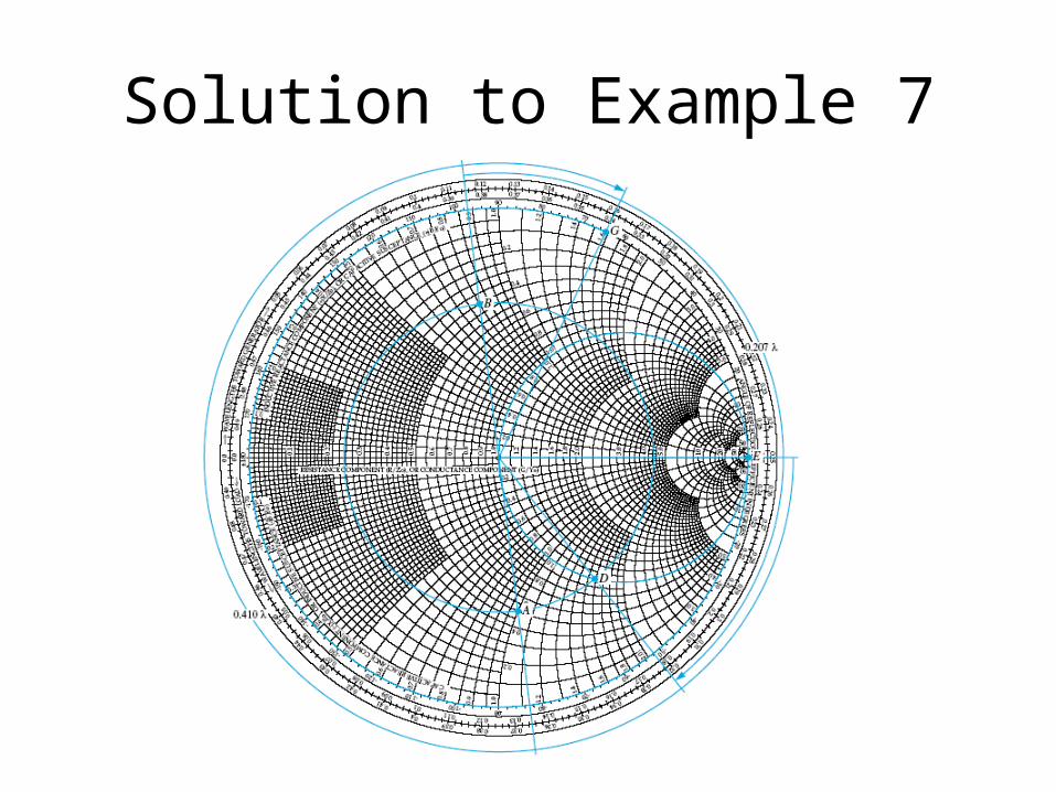
Solution to Example 7
• The normalized load impedance is
(located at A).
• Value of yL at B is which locates at position 0.115λ on the WTG scale.
• Draw constant SWR circle that goes through points A and B.
• There are two possible matching points, C and D where the constant SWR circle intersects with circle rL=1 (now gL =1 circle).
jj
Z
Zz
5.0
50
5025
0
LL
8.04.0L jy

Solution to Example 7

Solution to Example 7
First matching points, C.• At C, is at 0.178λ on WTG scale.• Distance B and C is• Normalized input admittance
at the juncture is:
E is the admittance of short-circuit stub, yL=-j∞.
Normalized admittance of −j 1.58 at F and position 0.34λ on the WTG scale gives:
58.11d jy 063.0155.0178.0 d
58.1
58.1101
s
s
sin
jy
jyj
yyy d
09.025.034.01 l

Solution to Example 7
Second matching point, D.• At point D,• Distance B and C is• Normalized input admittance at G. • Rotating from point E to point G, we get
58.11 jyd 207.0115.0322.02 d
58.1s jy
41.016.025.02 l
Solution to Example 7