Electromagnetic Modeling

2015 International Conference on Lightning and Static Electricity (Toulouse, France)

1

ELECTROMAGNETIC MODELING OF RETURN

CONDUCTOR CONFIGURATIONS USING THE FINITE

ELEMENT METHOD

Justin P. McKennon*

*Lightning Technologies, an NTS Company,USA. [email protected]

Keywords: Finite Element Analysis, Boundary Conditions,

COMSOL Multiphysics, Return Conductor

1 Abstract

Return conductor networks are typically used to provide a

low inductance return path back to the generator during most

full vehicle tests and tests of other large objects. There are

several commonly used methods of return networks, the most

popular of which are coaxial return arrays and ground planes.

During the construction of these arrays, practical

considerations often take precedence over the intended design

due to facility constraints, time, materials, and accessibility

issues. While conducting tests, it is not uncommon for wires

to be moved, droop, or fall, and the impact of these changes

on measurements and current flow is not well understood.

Utilizing the finite element method in COMSOL

Multiphysics, these effects can be accurately calculated. In

this work, a sample wing box is constructed in COMSOL

with several ribs and spars. A coaxial return array and ground

plane return network are modelled, with common routing and

configuration defects analyzed.

2 Introduction

The rationale for making use of a coaxial return array

configuration can be explained by examining the magnetic

fields within hollow conductors. If there are two conductors

carrying equal current in the same direction, the fields

produced by the two conductors cancel along a long

equidistant from the two conductors. The fields at other points

do not cancel, but their sum is lower than in the space outside

the conductors [1]. If there are three equally spaced parallel

conductors carrying equal currents, the fields are further

reduced in the intervening space between the conductors [1]

[2]. The more conductors carrying identical currents that are

arranged in a cylindrical configuration, the more magnetic

field cancellation occurs within the cylinder. If an infinite

number of parallel conductors are arranged in this

configuration so that they merge, forming a near solid tube,

the magnetic field due to currents on the tube becomes zero

everywhere inside the tube [1] [2]. Thus, by making use of

these principles, the impact of the return path on the test

object and measurements can be greatly reduced with the

aircraft or test object acting as the center conductor and the

return path as the outer conductor.

The further the return conductor array is from the surface of

the aircraft, the less the fields created by current travelling in

the conductor interact with the aircraft or test object inside the

array. However, due to practical limitations, the separation of

the wires is generally limited to 1-2 meters, which is a

common height that landing gear and test support objects are

able to raise the object above the ground. Wires are generally

held in place by return array stanchions such as those shown

below in Figure 1 [2].

Figure 1- Typical Stanchion Support of Return Conductors

Due to the randomness associated with taking measurements

(changes in applied current between injections, facility noise,

etc.) it is very difficult to characterize the influence of the

wires on the test object. Thus, in order to accurately

determine the influence of the return wires on the test object,

a geometrically accurate representation of the test setup must

be developed, including the array, and the fields and current

densities must be calculated.

Another common return network configuration involves the

use of a ground plane. Current is returned from the root of the

test object along a ground plane under the test object, which

connects to the generator to complete the circuit. Large test

objects often make use of this technique due to it being much

easier to implement than the return array. The intent of this

configuration is to minimize the influence of the return

current on the test object, due to the current density anywhere

in the ground plane being small [2].


2

Using software packages such as COMSOL Multiphysics,

highly accurate models of test objects (often derived directly

from Computer-Aided-Design (CAD) files) can be solved

analytically determining the field levels and current densities

associated with a test, without any of the issues associated

with noise or measurement challenges. COMSOL in

particular employs the Finite Element Method to solve

systems of partial differential equations that represent the

entirety of the physics interactions occurring in the model.

This paper focuses on the simulation and analysis of a

representative wing section in various return array

configurations through the use of the Finite Element Method

in COMSOL.

3 Model Development

3.1 Model Geometry

The model used in this work is that of a representative

aluminium wing section. The upper and lower wing skins are

both 0.2” thick, as are the forward and aft spars. Two

representative conductors are routed through the structure and

there are two apertures; one corresponding to an access panel

that may not be installed fully, and the second corresponding

to a NACA scoop as shown in Figure 2.

Figure 2 - Apertures in Geometry

200kA of the quad exponential analytical waveform for

Current Component A, defined in [3], is injected at 8 discrete

points intended to represent the redistribution of current that

occurs during an outboard wing tip strike. The injection

points are shown in Figure 3.

Figure 3 - Injection Points

Current flows through the wing structure and is removed at

the opposite end with connections to the return conductor

array. The ideal setup for the return array, in a pure coaxial

configuration – essentially an infinite number of infinitely

close return conductors, is shown in Figure 4.

Figure 4 - Ideal Return Array Setup

This configuration serves as the control for this research. The

effects of the return network on the test article are negated in

this configuration, allowing for the “True” values associated

with measurements to be obtained in this model.

3.2 Model Boundary Conditions

In order for the current density, electric fields, and magnetic

fields to be determined in an analytical model, proper

boundary conditions must be applied in order for the

governing mathematical equations to be solvable. This work

makes use of the Radio Frequency (RF) module in COMSOL

to do so. This work uses a 3D formulation of Maxwell’s

Equations to calculate the electromagnetic fields and current

densities, shown in Equation 1.

(1)

In (1), the magnetic vector potential, A, is solved for, and the

associated current densities and fields are determined. The

constitutive relations, and specific material parameters

(conductivity (σ), permittivity (ɛ), permeability (μ)), are

specified for each domain in the model. This allows for

different material types – aluminium, air, copper – to be

applied on various domains throughout the model to influence

the electromagnetic fields and flow of current accordingly.

One additional boundary condition is specifically used in this

model and warrants discussion. The Perfect Electrical

Conductor (PEC) boundary condition is applied

on all exterior surfaces to limit the solution to the model to a

finite size. This boundary condition sets the tangential

components of the electric potential to zero. It imposes

symmetry for electric and magnetic fields, and any current

flowing into a boundary with the PEC condition applied is

perfectly balanced by induced surface currents. This allows

for the PEC boundary condition to function as a way to


3

“Ground” the model and provide a way for any displacement,

conducted, and induced surface currents to be grounded. The

PEC boundary condition, in this work, is applied on all

exterior surfaces in the air domain of the model, as well as on

the connections to the return array conductors.

3.3 Mesh

The Finite Element Method is a numerical technique for

finding approximate solutions to systems of differential or

partial differential equations that are governed by boundary

conditions. At its core, the finite element method divides the

generated model geometry into smaller pieces – finite

elements – and uses variational methods to solve the problem

by minimizing the associated error function and achieve

convergence.

Once the geometry has been developed and the boundary

conditions have been applied, the model needs to be meshed.

COMSOL provides a robust, automatic meshing algorithm

that performs much of the meshing without need for user

input. Care must be taken to analyze the generated mesh and

ensure that sufficient mesh density exists in the regions of

interest in the model. The determination of the proper mesh

density falls outside the scope of this work. Using the

automatic meshing algorithm in COMSOL, Figure 5 is

produced.

Figure 5 - Meshed Model

4 Results

4.1 Nominal Coaxial Configuration

The wing model was first simulated in an ideal array

configuration, with no defects present in the geometry of the

return array to serve as a control for this work and provide a

basis for comparison. This configuration is a pure coaxial

geometry, with all of the current being returned along the

model boundaries to the current source. This is equivalent to

an infinite number of infinitely close return conductors.

Figure 6 shows the nominal configuration.

Figure 6 - Ideal Return Array

This configuration serves to demonstrate the current density

in the various components in the model, without the exterior

influence of any individual return conductors contributing to

the measurements. A plot of the current density, at 6.4 μS in

log base 10 scale, is shown in Figure 7.

Figure 7 - Current Density in Wing Box with Ideal Array

Configuration

As shown, the current density is concentrated at the edges of

the model. The skin effect, caused by the presence of eddy

currents in the Ribs, can also be seen in Figure 7.

Surface current density measurements in the upper wing skin,

FWD and AFT Spars, and on the lower wing skin near each

aperture were taken. The location of these measurements is

shown in blue in Figure 8. Figure 9 shows the measured

surface current densities at each location under the Ideal

Array Configuration.

Figure 8 - Surface Current Density Measurement Locations

on Exterior Surfaces


4

Figure 9 - Ideal Return Array Surface Current Density

Measurements

4.2 Array Configuration With Uniform Spacing

Since physical limitations (size, space, inductance, and

accessibility) prevent the use of the nominal configuration

shown in section 4.1, actual tests are run with a finite number

of conductors in the return array. The number of conductors

varies between individual tests and test articles; however the

most common array configuration involves several wires

encompassing the wing circumferentially. The configuration

used in this work has uniformly spaced conductors (in

relation to both the test object and one another). Each wire is

12 inches from the test article, and 18 inches from adjacent

wires. This spacing remains constant throughout the length of

the article, and is shown in Figure 10.

Figure 10 - Uniform Return Conductor Array Geometry

The same measurements described in section 4.1 were taken

with the uniformly spaced array conductors, and are shown in

Figure 11.

Figure 11 - Uniform Return Array Surface Current Density

Measurements

4.3 Array Configuration without Uniform Spacing

In order to take measurements during actual testing, parts of

the test article need to be opened, closed, moved, or altered. It

is not uncommon for the wires of the array to be moved

accidentally, or repositioned to accommodate personnel or

test equipment. Additionally, due to laboratory space and

inductance constraints, it may not be possible to uniformly

space the conductors. In Figure 12, a random, 10% variation

in conductor-to-conductor and conductor-to-test-object

spacing is introduced. This randomly displaces each of the

wires in the array from their uniform locations.

Figure 12 - Random Spaced Conductor Geometry

Figure 13 shows the surface current waveforms in this

configuration.

Figure 13 - Non-Uniform Return Array Surface Current

Density Measurements


5

4.4 Array Configuration with Uniform Spacing and

Sagging Wires

During some tests, it is not uncommon for individual wires in

the array to sag or droop. When this happens, the rest of the

array can stay intact (with the intended spacing), but one or

multiple wires can hang closer to, or further away from, the

test article. This is most common on wires routed along the

upper wing skin (wire sags closer to the surface) and lower

wing skin (wire sags further away from surface). Figures 14

and 15 show the sagging wires in this configuration. In each

case, the wire is sagging 4 inches from the uniform

configuration. Figures 16 and 17 show the surface current

density measurements in each configuration.

Figure 14 - Wire Sagging Away from Lower Wing Skin

Figure 15 - Wire Sagging Towards Upper Wing Skin

Figure 16 - Wire Sagging Away from Lower Wing Skin

Surface Current Density Measurements

Figure 17 - Sagging Wire Towards Upper Wing Skin Surface

Current Density Measurements

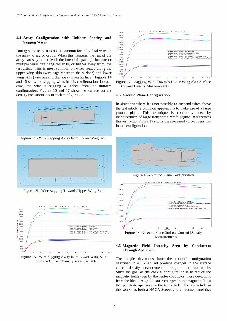
4.5 Ground Plane Configuration

In situations where it is not possible to suspend wires above

the test article, a common approach is to make use of a large

ground plane. This technique is commonly used by

manufacturers of large transport aircraft. Figure 18 illustrates

this test setup. Figure 19 shows the measured current densities

in this configuration.

Figure 18 - Ground Plane Configuration

Figure 19 - Ground Plane Surface Current Density

Measurements

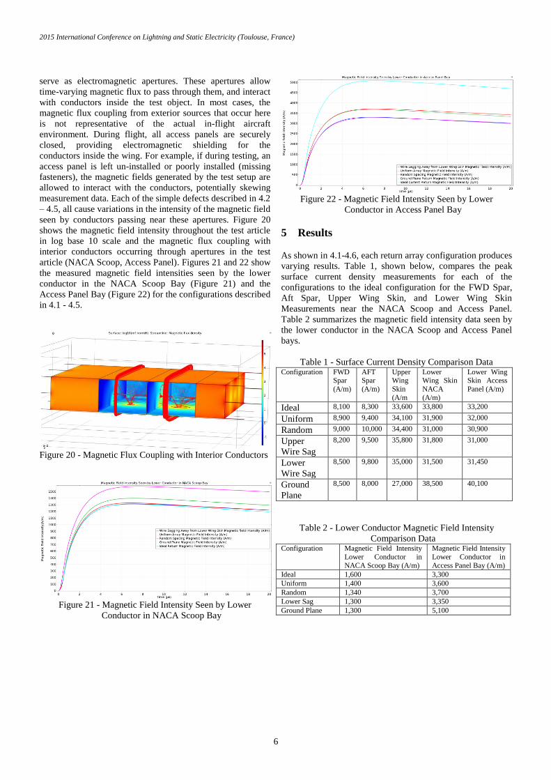
4.6 Magnetic Field Intensity Seen by Conductors

Through Apertures

The simple deviations from the nominal configuration

described in 4.1 - 4.5 all produce changes in the surface

current density measurements throughout the test article.

Since the goal of the coaxial configuration is to reduce the

magnetic fields seen by the center conductor, these deviations

from the ideal design all cause changes in the magnetic fields

that penetrate apertures in the test article. The test article in

this work has both a NACA Scoop, and an access panel that


6

serve as electromagnetic apertures. These apertures allow

time-varying magnetic flux to pass through them, and interact

with conductors inside the test object. In most cases, the

magnetic flux coupling from exterior sources that occur here

is not representative of the actual in-flight aircraft

environment. During flight, all access panels are securely

closed, providing electromagnetic shielding for the

conductors inside the wing. For example, if during testing, an

access panel is left un-installed or poorly installed (missing

fasteners), the magnetic fields generated by the test setup are

allowed to interact with the conductors, potentially skewing

measurement data. Each of the simple defects described in 4.2

– 4.5, all cause variations in the intensity of the magnetic field

seen by conductors passing near these apertures. Figure 20

shows the magnetic field intensity throughout the test article

in log base 10 scale and the magnetic flux coupling with

interior conductors occurring through apertures in the test

article (NACA Scoop, Access Panel). Figures 21 and 22 show

the measured magnetic field intensities seen by the lower

conductor in the NACA Scoop Bay (Figure 21) and the

Access Panel Bay (Figure 22) for the configurations described

in 4.1 - 4.5.

Figure 20 - Magnetic Flux Coupling with Interior Conductors

Figure 21 - Magnetic Field Intensity Seen by Lower

Conductor in NACA Scoop Bay

Figure 22 - Magnetic Field Intensity Seen by Lower

Conductor in Access Panel Bay

5 Results

As shown in 4.1-4.6, each return array configuration produces

varying results. Table 1, shown below, compares the peak

surface current density measurements for each of the

configurations to the ideal configuration for the FWD Spar,

Aft Spar, Upper Wing Skin, and Lower Wing Skin

Measurements near the NACA Scoop and Access Panel.

Table 2 summarizes the magnetic field intensity data seen by

the lower conductor in the NACA Scoop and Access Panel

bays.

Table 1 - Surface Current Density Comparison Data Configuration FWD

Spar

(A/m)

AFT Spar

(A/m)

Upper Wing

Skin

(A/m

Lower Wing Skin

NACA

(A/m)

Lower Wing Skin Access

Panel (A/m)

Ideal 8,100 8,300 33,600 33,800 33,200

Uniform 8,900 9,400 34,100 31,900 32,000

Random 9,000 10,000 34,400 31,000 30,900

Upper

Wire Sag

8,200 9,500 35,800 31,800 31,000

Lower

Wire Sag

8,500 9,800 35,000 31,500 31,450

Ground

Plane

8,500 8,000 27,000 38,500 40,100

Table 2 - Lower Conductor Magnetic Field Intensity

Comparison Data Configuration Magnetic Field Intensity

Lower Conductor in

NACA Scoop Bay (A/m)

Magnetic Field Intensity

Lower Conductor in

Access Panel Bay (A/m)

Ideal 1,600 3,300

Uniform 1,400 3,600

Random 1,340 3,700

Lower Sag 1,300 3,350

Ground Plane 1,300 5,100


7

6 Conclusion

In this work, several common return array configurations

were examined. An ideal coaxial return arrangement, in

which the magnetic fields generated by the return conductors

are very low, serves as the control for this research. Since the

ideal array is not attainable, the currently accepted best

practice is to uniformly space several conductors

circumferentially around the wing. Comparing the surface

current density measurements between the ideal and realistic

return arrays shows that the uniform configuration can serve

as an appropriate return configuration. With variations in the

surface current density measurements being less than 2,000

A/m between the two, in addition to comparable magnetic

field intensity measurements, it is reasonable to state that

measurements taken within a uniform return configuration are

acceptable. The ground plane return configuration produces a

significantly different current distribution, skewed towards

the lower wing skin area. Since the return is below the test

object, the path of least resistance is through the lower skin,

which explains the increased current density and magnetic

field readings.

However, as defects are introduced into the uniform array, be

it through improper spacing or sagging wires, the surface

current density also changes. With a variability in spacing

(conductor to conductor /conductor to test object) of 10% (or

less than 2 inches), the current density measurements change

by several hundred A/m (for a 200kA test current). During

actual testing, these distances can certainly be larger than 2

inches (from the uniform location), and the impacts of these

non-uniformities will continue to increase, especially near

apertures.

To summarize, the currently accepted method of a coaxial

return array provides a suitable return path for the current,

with minimal impact on the test object and measurements.

Deviations from this uniform array do have an impact

proportional to the distance the wire is located away from its

uniform (intended) location.

Poorly constructed arrays, or arrays that have been

unintentionally modified during testing, can skew data and

yield potentially misleading data as a result. Care must be

taken to ensure that the array stays in the uniform

configuration as much as possible, as deviations in return

conductor routing locations will alter current flow and impact

measurement data, providing an unrealistic aircraft

environment.

7 References

[1] Wieting, T, et al.: ‘Electromagnetic Field

Investigations Inside a Hollow Cylinder’,

International Journal for Computation and

Mathematics in Electrical and Electronic

Engineering, April 1995, pp. 223-227

[2] Fisher, F., Perala R., and Plumer, J.A.: ‘Lightning

Protection of Aircraft’ (Lightning Technologies,

2004, 2nd

edn)

[3] SAE ARP 5412B: ‘ Aircraft Lightning Environment

and Related Test Waveforms’, 2013

Electromagnetic Modeling

Documents

Transcript of Electromagnetic Modeling