Electrochemical Speciation and Quantitative Chromatography

for Modelling of Indium Bioleaching Solutions

From the Faculty of Chemistry and Physics

of the Technische Universität Bergakademie Freiberg

is approved this

THESIS

to attain the academic degree of

Doctor rerum naturalium

(Dr. rer. nat)

submitted by MChem. Charlotte Victoria Ashworth

born on the 17th May 1991 in Crewe, England

Supervisors: Prof. Gero Frisch, Technische Universität Bergakademie Freiberg

Prof. Karl Ryder, University of Leicester

Awarded on 06.09.2018

Declaration

I hereby declare that I completed this work without any improper help from a third party and

without using any aids other than those cited. All ideas derived directly or indirectly from other

sources are identified as such.

I did not seek the help of a professional doctorate-consultant. Only persons identified as having

done so received any financial payment from me for any work done for me.

My thesis has not previously been submitted to another examination authority in the same or

similar form in Germany or abroad.

Freiberg, 09.07.2018

i

Parts of this work have been published in the following paper:

Ashworth, Frisch. 2017. “Complexation equilibria of indium in aqueous chloride, sulfate and

nitrate solutions: An electrochemical investigation.” Journal of Solution Chemistry 46 (9):

1928–40.

This work has also been presented at the following conferences:

Presentations

- Electrochemical speciation measurements for geochemical modelling of leachate

solutions, BHT, Freiberg, 2018

- Electrochemical speciation measurements for quantitative analysis of polymetallic

solutions, AKES, Freiberg, 2018

- Complexation equilibria of indium in aqueous sulphate, chloride, and nitrate solutions,

AKES, Chemnitz, 2017

- Speciation and electrochemistry of indium in aqueous sulfate and chloride solutions,

ISSP-17, Geneva, 2016

- Untersuchungen zu Elektrochemie und Speziation des Indiums in sauren

Laugungslösungen, BHT, Freiberg, 2015

Posters

- The electrochemically active speciation of indium in aqueous sulphate and chloride

solutions, MANS-14, Halle, 2016

- The effect of ligand competition on the speciation and electrochemical behaviour of

indium in acidic solutions, GDCh-Wissenschaftsforum, Dresden, 2015

- The effect of ligand competition on the speciation and electrochemical behaviour of

indium in acidic solutions, MANS-13, Chemnitz, 2015

- The effect of inorganic acids on the electrodeposition of indium, MANS-12, Freiberg,

2014

ii

Acknowledgements

I would like to thank my supervisor Prof. Gero Frisch, without whom I would not be here,

either professionally or geographically. I am incredibly grateful for your patience, guidance,

and advice both here and in Leicester.

Additionally, many thanks to Prof. Karl Ryder for agreeing to be my second examiner.

I am grateful for the generous funding of the Dr. Erich Krüger Foundation, without which this

research would not have been possible. For their help and support I would also like to thank

the Salt and Mineral Chemistry work group and the Biohydrometallurgical Centre Freiberg.

Thanks also to new friends and neighbours here in Germany: the Frisch family for taking me

in, and Phil for taking me out. As well as old friends from home, especially Steph for nodding

patiently while I complained about science.

For all types of support other than scientific, I must thank my family, I could not have done it

without the constant encouragement and enthusiasm. Thank you for believing in me.

Finally I want to thank my fiancé Freddy, whether it was motivation or commiseration, you

always kept me going. Thank you for helping me get through this.

iii

Abstract

Since 2011, indium has been considered a critical raw material due to its economic importance

and supply risk. In order to meet future challenges, especially regarding processing of low-

grade resources, (bio)hydrometallurgical approaches to metal winning are likely to play a

significant role. Hence the Biohydrometallurgical Centre (BHMZ) was established to research

the entire biohydrometallurgical process chain for winning of indium from local sphalerite. The

focus of this work within the scope of the BHMZ was the development of methods to a)

determine indium stability constants, and b) quantify metal ions and sulfur species expected in

the leachate by the polysulfide leaching pathway of sphalerite. Including these results in

geochemical models can then allow the prediction of speciation, and hence chemical behaviour,

of target metals in leaching and extraction solutions.

A differential pulse voltammetry method was adapted to simultaneously determine indium

speciation and complex stability. The stability constants of indium complexes with nitrate,

chloride, and sulfate ions, as well as indium hydrolysis constants, were determined. This

method was also applied to extraction solutions where the stability of indium with

electrowinning additives was determined.

With ion chromatography it was possible to simultaneously quantify indium, copper, zinc,

nickel, manganese, and ferric and ferrous iron in a number of process relevant solutions.

Increasing column temperature to 45 ºC solved the co-elution of In3+ and Cu2+. Indium peak

splitting was explained by establishing the stability of indium in these measurements and

solved by diluting samples in the chromatographic eluent. High pressure liquid

chromatography was used to quantify polysulfides (Sx2–). A capping procedure to preserve

unstable polysulfides allowed separation and detection of polysulfide chains up to S82–, and an

average total polysulfide concentration of 12.5 µmol/kg was found in leachate samples.

This cumulative information was used in geochemical modelling to study indium behaviour in

model solutions, as well as leachate and extraction solutions under various conditions (pH,

redox potential, and temperature). Predominance, Pourbaix, and speciation diagrams were

constructed to describe and explain the behaviour of multiple components in various process

relevant solutions.

iv

Abbreviations

AMD acid mine drainage

CIGS copper indium gallium selinide

CRM critical raw material

CV cyclic voltammogram

DPV differential pulse voltammogram

EOL end of life

EXAFS extended x-ray absorption fine structure

GCE glassy carbon electrode

HMDE hanging mercury dropping electrode

HPLC high pressure liquid chromatography

IC ion chromatography

ITO indium tin oxide

LCD liquid crystal display

NPV normal pulse voltammetry

PGM platinum group metals

ppm parts per million

PLS pregnant leach solution

QCM quartz crystal microbalance

REE rare earth elements

SMDE / DME (static) mercury dropping electrode

Subscripts

a anodic

c cathodic

f free

com complexed

red reduced species

ox oxidised species

surf at electrode surface

bulk in bulk solution

p peak

lim diffusion limited

tot total

v

Symbols

α charge transfer coefficient

βx cumulative stability constant

δ diffusion layer thickness cm

ε molar absorption coefficient mol–1 L cm–1

η overpotential V

λ wavelength nm

μq shear modulus 2.947 × 1011 g cm–2 s–2

ρq density quartz 2.648 g cm–3

τ time delay after potential pulse s

υ scan rate V s–1

A area cm–2

Abs absorbance

c concentration mol kg–1 / mg L–1

C charge C

D diffusion coefficient cm2 s–1

E electrode potential V

E1/2 half wave potential V

ΔE potential pulse amplitude V

f frequency Hz

F Faraday constant 96,485.3329 C mol–1

G Gibbs free energy J mol–1

H enthalpy J mol–1

i current A

i0 exchange current A

I ionic strength mol kg–1

j current density A cm–2

k rate constant s–1

Kx stepwise stability constant

Kw ionic product of water

Ksp / K*sp solubility product

l length cm

m mass g

mHg mercury flow rate mg s–1

M molar mass g mol–1

vi

n number of electrons

Q reaction quotient

r bond length Å

R gas constant 8.314 J K–1 mol–1

S entropy J K–1 mol–1

t time s

T temperature K

x number of ligands

[M] / [L] concentration of metal ion / ligand mol kg–1 / mg L–1 [M(H2O)x] /

[MLx] concentration of hydrated metal ion /

metal-ligand complex mol kg–1 / mg L–1

Contents

Acknowledgements……………………………………………………………………………ii

Abstract……………………………………………………………………………………….iii

Abbreviations…………………………………………………………………………………iv

Chapter One – Introduction

1. Indium

1.1. Discovery, Occurrence, and Applications…………………………………………1

1.2. Properties and Compounds………………………………………………………..2

1.3. Availability, Production, and Demand…………………………………………….4

2. The Biohydrometallurgical Centre for Strategic Elements

2.1. Aims of the BHMZ………………………………………………………………..9

2.2. Hydrometallurgy…………………………………………………………………10

2.3. Biohydrometallurgy……………………………………………………………...12

2.4. Aims of this Work………………………………………………………………..16

3. Theoretical Background

3.1. Equilibrium Constants…………………………………………………………...19

3.2. Spectroscopic and Electrochemical Experimental Techniques…………………..27

3.3. Polarography……………………………………………………………………..33

3.4. Differential Pulse Voltammetry………………………………………………….37

3.5. Techniques to Determine Diffusion Coefficients………………………………..44

3.6. Geochemical Modelling…………………………………………………………46

3.7. Chromatographic Methods………………………………………………………49

Chapter Two – Establishment of Techniques and Application to Model Solutions

4. Spectroscopic and Electrochemical Behaviour of Indium

4.1. Spectroscopic Measurements…………………………………………………….53

4.2. Electrochemical Measurements………………………………………………….58

4.3. Summary of Qualitative Spectroscopic and Electrochemical Analyses………….64

5. Determining Indium Stability Constants

5.1. Differential Pulse Voltammetry Titration Technique…………………………….67

5.2. Indium Complexation with Sulfate………………………………………………71

5.3. Indium Complexation with Chloride…………………………………………….74

5.4. Indium Complexation with Hydroxide…………………………………………..75

5.5. Summary of Quantitative Determination of Indium Speciation and Stability……81

6. Geochemical Modelling

6.1. Modelling of Indium Complexation with Nitrate, Sulfate, and Chloride………..83

6.2. Modelling of Indium Hydrolysis…………………………………………………87

6.3. Summary of Geochemical Modelling of Model Indium Solutions………………93

7. Chromatographic Methods

7.1. Determining Sulfur Species with High Pressure Liquid Chromatography….……94

7.2. Determinging Metal Ion Concentration with Ion Chromatography……..……….98

7.3. Summary of Chromatographic Analyses of Model Indium Solutions…………..102

Chapter Three – Application to Project Relevant Samples

8. Analysis of Leachate Solutions

8.1. Detection of Polysulfides in Leachate Solutions…..…………………………....106

8.2. Determining Metal Ion Concentrations in Leachate Solutions..………………...108

8.3. Geochemical Modelling of Leachate Solutions……..…………………………..112

8.4. Application of Analysis Methods to Leachate Solutions…..……………………121

9. Analysis of Membrane Filtration Solutions

9.1. Determining Metal Ion Concentrations in Membrane Filtration Solutions….….122

9.2. Geochemical Modelling of Membrane Filtration Solutions…………………….124

9.3. Electrochemical Determination of Diffusion Coefficients……………………...128

9.4. Application of Analysis Methods to Membrane Filtration Solutions………...…132

10. Analysis of Electrowinning Solutions

10.1. Stability and Speciation of Indium in Electrowinning Solutions………………133

10.2. Application of Analysis Methods to Electrowinning Solutions………………..136

Chapter Four – Summary and Conclusions

11. Summary and Conclusions

11.1. Motivations……………………………………………………………………137

11.2. Technique Development and Application to Model Solutions………………...138

11.3. Application to Process Relevant Solutions…………………………………….142

Appendix

i. Experimental Methods…………………………………………………………….146

ii. PHREEQC Input Files……………………………………………………………154

iii. List of Tables and Figures………………………………………………………..162

References…………………………………………………………………………………..168

1

Chapter One – Introduction Indium is an essential component in a number of thin film applications and the tenfold increase

in demand predicted in the next 25 years cannot be satisfied by current production methods

[Angerer 2009; White and Hemond 2012]. Indium is typically recovered as a by-product during

smelting of sulfidic ores to produce zinc, hence indium production is dependent on zinc

manufacturing rates, rather than indium demand. Access to minerals containing high indium

concentrations is becoming increasingly challenging and current pyrometallurgical methods

cannot efficiently process these complex or low-grade sources of indium. Alternative

processing methods based on hydro- and biohydrometallurgical techniques could be an

effective alternative.

The Biohydrometallurgical Centre Freiberg (BHMZ) was established to develop a process

chain for in-situ bioleaching, where bacteria catalyse the oxidation of sulfidic minerals, to win

indium from local ores. The contribution of this work was to determine equilibrium constants

of indium under relevant hydrometallurgical conditions. Due to the sulfidic ore, interactions

between indium and sulfate will be of particular importance, but indium complexation with

nitrate and chloride will also be investigated. These constants can then be used by geochemical

modelling software to determine speciation, and hence chemical behaviour, of target metals in

leaching and extraction solutions.

The first part of chapter one will summarise the chemistry of indium and include an overview

of hydro- and biohydrometallurgy. The goals of the BHMZ project and the aims of this work

will be presented in the second section. A review of the theoretical fundamentals regarding

equilibrium constants, as well as the experimental techniques used to determine them in this

work is discussed in section 3.

1. Indium

1.1. Discovery, Occurrence, and Applications

Indium is considered a strategically important element due to its widespread use in electronic

devices. Indium tin oxide (ITO) is an essential component of solar panels and liquid crystal

displays (LCDs) and since 1992, thin-films have been the most significant application of

2

indium [Directorate-General for Internal Market, Industry, Entrepreneurship and SMEs 2017].

Its electrical conductivity, environmental resistance, low melting point, and ability to wet glass

makes ITO highly useful for thin film applications [Kim, Gilmore et al. 1999; George 2004].

Indium nitride, phosphide, and antimonide are semiconductors used in transistors and

microchips [Downs 1993; Alfantazi and Moskalyk 2003; Liu, Avrutin et al. 2010] and copper

indium gallium selenide (CIGS) is used for thin film solar cells [Powalla and Dimmler 2000].

Indium is the 68th most abundant element in the Earth's crust with a concentration of

approximately 50 ppb [Emsley 1999]. The abundance is similar to silver, bismuth, or mercury

[Hedrick 1999]. Indium minerals such as roquesite (CuInS2), cadmoindite (CdIn2S4), and indite

(FeIn2S4) are rarely formed and do not occur at concentrations sufficient for economical

extraction. Indium is often a trace constituent of minerals such as sphalerite (ZnS) [Frenzel,

Hirsch et al. 2016] where it deposits via ionic substitution of zinc [Bauer, Seifert et al. 2017].

Incorporation of indium in the sphalerite lattice proceeds via the coupled substitution

Cu+ + In3+ ⇌ 2 Zn2+ [Cook, Ciobanu et al. 2009]. However, copper and indium concentrations

in sphalerite are not always equal indicating this is not the only ionic substation reaction

occurring. The general co-substitution mechanism for trivalent ions has been presented:

M (I) + M (III) ⇌ 2 Zn (II), where M (I) = Cu and M (III) = In, Fe [Johan 1988].

Concentrations of indium in sphalerite are typically below 100 ppm [Graeser 1969; Grafenauer,

Gorenc et al. 1969], an average of the estimated indium content in zinc ores processed in 2009

was 26 ppm [Lokanc, Eggert et al. 2015].

Indium was discovered in 1863 by F. Reich and H. T. Richter of the TU Bergakademie

Freiberg. Spectral analysis of local pyrite, galena, and sphalerite ore was expected to include

the green emission line of thallium. Instead, a previously unidentified bright blue line was

found and thus the presence of an undiscovered element was proposed. The name indium

comes from the distinct indigo colour of its emission spectrum [Reich and Richter 1863].

1.2. Properties and Compounds

Indium is a post-transition metal chemically similar to gallium and thallium. According to its

position in the periodic table, the properties of indium are typically an intermediate between

the two. For example, from the valence electron configurations of gallium, indium, and

thallium (4d10 5s2 5p1), it is logical that the +3 and +1 cations are stable. Gallium commonly

3

only shows the Ga3+ oxidation state, In3+ is stable but under certain conditions In+ can also be

formed, whereas Tl+ is more likely to form than Tl3+ [Holleman, Wiberg et al. 2007].

Indium (III) oxide, In2O3, is formed when indium metal is burned in air or when the hydroxide

or nitrate is heated [Downs 1993]. Indates are produced from reactions with alkalis and

reactions with acids produce indium salts (e.g. In(OH)3 + 3 HCl → InCl3 + 3 H2O). Indium

trihalides are Lewis acids chemically similar to aluminium trihalides. Indium (I) compounds

are not common. Indium (I) oxide is produced when indium (III) oxide decomposes upon

heating above 700 °C [Downs 1993]. Even less frequently indium forms compounds in a +2 or

even fractional oxidation states, usually with In–In bonding, most notably in the halides In2X4

[Sinclair and Worral 1982].

The In3+ cation is classified as a hard Lewis acid due to its high charge, small size, and

symmetrical d10 valence electrons [Petrosyants and Ilyukhin 2011]. The In3+ ion forms a hexa-

aqua complex in water [In(H2O)6]3+ where metal-ligand complex formation occurs via ligand

substitution. In3+ forms strongly bonded coordination complexes with hard donor atoms such

as N, O and F, as well as some softer bases like P, S, and Cl. At increasing pH values associated

water molecules are deprotonated to form indium hydroxides, InOH2+ and In(OH)2+, eventually

forming neutral and highly insoluble In(OH)3, In(OH)4– is only formed at very high pH values.

1.2.1 Electrochemistry of Indium

A brief summary of the electrochemistry of indium will be given here, thorough evaluations

have been carried out in reviews by [Chung and Lee 2012] and [Piercy and Hampson 1975].

From the electron configuration of indium ([Kr] 4d10 5s2 5p1) it can be assumed that trivalent

indium compounds are stable. They are most commonly formed, however occasionally the

5s electrons are not donated, resulting in the less stable In+ cation. The ionisation potentials for

the three valence electrons are approximately 5.78, 18.87, and 28.03 eV for the 5p1, 5s2, and

5s1 electrons respectively [Piercy and Hampson 1975].

Electrochemical analysis of indium began with the determination of the deposition and

stripping mechanism of the In3+/0 redox pair. Groups such as [Lovrecek and Markovac 1962],

who studied variations in overpotential from indium amalgams, and [Losev and Molodov 1960]

who used labelled indium, initially proposed that the redox mechanism consisted of three

consecutive electron transfer steps. Where the rate determining step for both the anodic and

4

cathodic reactions was the electron transfer In3+ + e– ⇌ In2+. However, [Biederman and Wallin

1960], supported the presence of an In+ ion but could find no evidence indicating the existence

of the In2+ species. It is now known that the reduction of In3+ and the dissolution of metallic

indium occur via two charge-transfer steps with In+ as the intermediate ion. [Markovac and

Lovrecek 1965] later hypothesised that the rate limiting step for the cathodic reduction of

indium is the two electron transfer In3+ + 2 e– ⇌ In+, whereas for the anodic dissolution of

indium metal, the first step In + e– ⇌ In+ is rate limiting.

The standard reduction potentials of the In3+/0, In3+/+ and In+/0 couples have been determined by

various methods [Hakomori 1930; Bard and Parsons 1985; Visco 1965]:

In3+ + 2 e− ⇌ In+

In3+ + 3 e− ⇌ In

In+ + e− ⇌ In

𝐸𝜃 = −0.444 𝑉

𝐸𝜃 = −0.338 𝑉

𝐸𝜃 = −0.126 𝑉

(1)

(2)

(3)

The standard reduction potentials show that metallic indium is easier to oxidise to In3+ than In+.

The relationship between Gibbs energy and potential (ΔGϴ = –nFΔEϴ) can be used to show

that the disproportionation of the monovalent ion is energetically favourable as a positive value

for ΔEϴ results in a negative Gibbs energy.

Red: 2 In+ + 2 e− ⇌ 2 In 𝐸𝜃𝑟𝑒𝑑 = −0.126 𝑉 (4)

Ox: In+ ⇌ In3+ + 2 e− 𝐸𝜃𝑜𝑥 = −0.444 𝑉 (5)

3 In+ → 2 In + In3+ ∆𝐸𝜃 = +0.318 𝑉 (6)

∆𝐺𝜃 = −61.4 kJ mol−1

Hence the focus of this work will be on complexes formed with the aqueous In3+ ion and,

specifically regarding electrochemical investigations, the In3+/0 redox couple.

1.3. Availability, Production, and Demand

Indium is mostly produced as a by-product of pyrometallurgical zinc sulfide ore processing.

Hence indium production depends on the amount of sphalerite processed to manufacture zinc,

rather than the actual demand for indium. Recent estimates put the supply potential of indium

at a minimum of 1,300 t per year from sulfidic zinc and 20 t per year from sulfidic copper ores

5

[Frenzel, Hirsch et al. 2016]. This is significantly greater than current production rates which

reached 655 t in 2016. China is the leading producer of indium (290 t in 2016), followed by

South Korea (195 t), Japan (70 t), and Canada (65 t) [Tolcin 2017]. In 2016 the average indium

price was $240/kg, dramatically reduced from $705/kg in 2014 [Kelly and Matos 2015].

About 90 % of zinc refining is done through hydrometallurgical processes in four general

stages:

1. The Waelz process – a mixture of zinc concentrates and coal is heated to produce a

calcine of impure zinc oxide

2. Leaching – the calcine is leached with sulfuric acid forming a zinc sulfate solution

3. Cementation – precipitation of valuable noble metals with zinc or iron powder

4. Electrowinning – zinc is deposited on an aluminium cathode, where it can be

mechanically removed, melted, and cast into ingots.

Indium and other elements such a copper, cadmium, germanium, and gallium can be recovered

during cementation. Specific information regarding refinery technology is difficult to acquire

due to the proprietary nature of such processes, however a general summary of indium refining

is shown in Figure 1 using typical values and descriptions from Ullmann’s encyclopaedia [Felix

2002] and information provided by indium manufacturers [Fthenakis, Wang et al. 2009].

Low economic advantages to zinc producers, as well as complex extraction processes, typically

makes rates of indium recovery relatively poor. Typically, less than 20 % of the indium content

of concentrates is extracted to yield pure indium metal [Mikolajczak 2010]. However, higher

indium prices and technological developments are making it more economically viable for

mines, smelters, and refineries to invest in increasing yields and capacities.

7

and 62 % of the EU supply [European Commission 2014]. The European Commission has

created a list of Critical Raw Materials (CRMs) which combine a significant economic

importance to the EU with a high risk associated with their supply. The goal is to increase

awareness of potential supply risks, encourage efficient use of these materials, and stimulate

production by enhancing new mining and recycling activities. Indium has been designated a

CRM since the first report in 2011 [European Commission 2011].

1 2 3 4 5 6 70

1

2

3

4

5

Sb

Be

Bi

CoGa

Ge

Hf

Nb

P

Sc

V

HREEs

PGMs

Al

Cr

Kaoline clayMagnesite

Mn

Ni

Potash

Re

Sapele wood

Silica sandAgTalc

Te Sn

Zn

Ta

Borate

In

BentoniteAggregatesAu

GypsumPerlite

Feldspar

Ti

PbDiatomite

Natural rubber

SeS

Cu

Bauxite

Natural cork

LiCoking coal

Natural teak wood

Limestone

Iron oreMo

W

Mg

HeBaryte

Si

LREEs

Phosphate rock

Sup

ply

Ris

k

Economic Importance

Natural graphite

Figure 2: Raw materials considered by the 2017 report with highlighted CRMs

REE: rare earth elements, PGM: platinum group metals

In 2017 an assessment of 78 materials was carried out [European Commission 2017], the results

are shown in in Figure 2, critical raw materials with high economic importance and supply risk

are highlighted in the upper right portion of the graph. Additionally, the list of 26 CRMs from

this study can be seen in Table 1.

Table 1: List of CRMs designated by the EU commission in 2017

REE: rare earth elements, PGM: platinum group metals

Antimony Baryte Beryllium Bismuth Borate

Cobalt Fluorspar Gallium Germanium Hafnium

Helium Heavy & Light REEs Indium Magnesium Natural

Graphite Natural Rubber Niobium PGMs Phosphate Rock Phosphorus

Scandium Silicon Metal Tantalum Tungsten Vanadium

8

A complementary report from [Bertrand, Cassard et al. 2016] produced a map showing

European mineral deposits containing CRMs, from the EU FP7 ProMine project database, with

respect to the 2014 EU report on CRMs. Deposit size classes A, B and C (super large, large,

and medium deposits respectively) are thresholds defined for each CRM individually. For

indium, a medium, large, and super large deposit contains at least 25, 100, and 500 metric tons

of indium respectively. The only super large indium deposit in Europe is located in Germany.

An additional large indium deposit can be found in Portugal.

Figure 3: Map showing mineral deposits containing CRMs in Europe [Bertrand, Cassard et al. 2016]

The demand for new and efficient indium production methods, coupled with the location of

both the discovery of indium, and indium containing mineral deposits, prompted the TU

Bergakademie Freiberg, with funding from the Dr. Erich Krüger Foundation, to establish the

Biohydrometallurgical Centre for Strategic Elements (BHMZ). The goal was to support the

supply of strategically important indium using hydrometallurgical and especially

biohydrometallurgical approaches to metal winning.

9

2. The Biohydrometallurgical Centre for Strategic Elements

This section will discuss the motivations and aims of the Biohydrometallurgical Centre as well

as introduce hydro- and biohydrometallurgical metal processing methods, which both play an

important role in the BHMZ process chain. In the conclusion of this section the specific aims

of this work within the scope of the BHMZ will be presented.

2.1. Aims of the BHMZ

Current indium production methods will not likely support predicted increases in demand

[Schwarz-Schampera and Herzig 2002; Hoffmann 1992]. Thus, lower grade or more complex

indium sources must now be exploited. Modern mining practices strive to minimise energy

consumption while also meeting high environmental standards, in this regard

hydrometallurgical techniques can be more efficient than traditional pyrometallurgy.

The goal of the BMHZ was to apply a specific branch of hydrometallurgy, called

biohydrometallurgy, where the oxidation of minerals is catalysed by specialised bacteria.

Through interdisciplinary collaboration, the best methods to bring metals from various source

materials (mineral deposits, tailings, heaps, and recycling materials) into aqueous solution will

be determined. Furthermore, various approaches to obtain pure metals from the leachate will

be investigated. Overall, the BHMZ aims to promote research into environmentally acceptable

mining of strategically important metals such as indium.

Figure 4 describes the proposed BHMZ process chain. As leaching of both ore bodies (in-situ)

and tailings (heap leaching) will be considered, expertise regarding both surface and sub-

surface mining is required. Microbiologists will identify and cultivate bacteria suitable for

leaching. In this work resulting leachates will be analysed and information applied to

geochemical modelling to determine the most efficient conditions for subsequent indium

extraction. Solvent extraction will yield indium salts which can be dissolved in electrolyte

solutions for the electrowinning of pure indium metal. A variety of groups with a range of

specialities are contributing to the BHMZ, allowing interdisciplinary research along the entire

process chain (see Figure 4).

10

Figure 4: A schematic of the proposed BHMZ process chain with the related contributing groups

2.2. Hydrometallurgy

Hydrometallurgy is an extractive metallurgical technique where aqueous chemistry is used for

the recovery of metals from ores, concentrates, and recycled materials [Habashi 2005].

Typically the process is divided into three stages [Woollacott and Eric 1994]:

1. Leaching – use of aqueous solutions to extract metals from target metal containing

minerals, concentrates, wastes, etc. Leaching solutions vary in terms of pH, redox

potential, temperature, and presence of chelating agents, to optimise rate and selectivity

of the leach. Four common leaching configurations are heap, tank, autoclave, and in-

situ leaching.

2. Concentration and purification – after leaching the resultant leachate or pregnant leach

solution (PLS) is often dilute with respect to target metals and must undergo

concentration and removal of undesirable contaminants. A combination of

precipitation, cementation, solvent extraction, ion-exchange, and electrowinning

processes are usually used to extract target metals or concentrate them in the PLS.

3. Metal recovery – raw materials can be produced in the metal recovery step, however,

sometimes further refinement is required, usually via precipitation [Han, Kondoju et al.

2002] or electrolysis [Lee and Oh 2004].

11

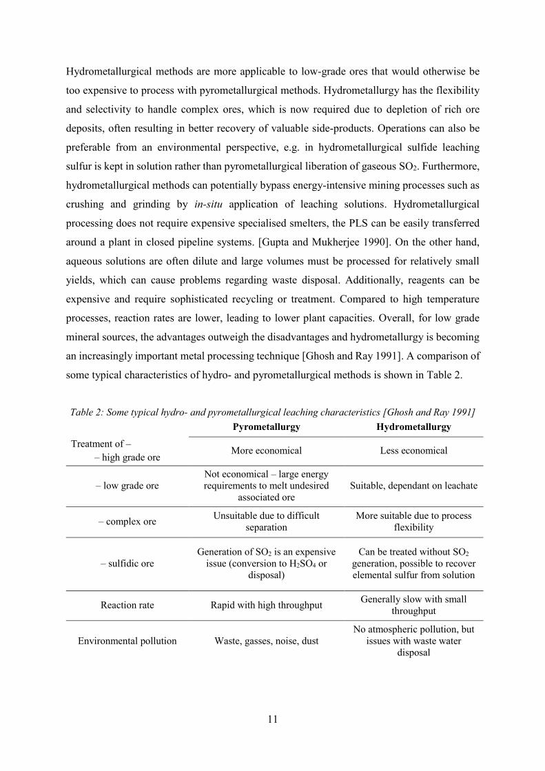
Hydrometallurgical methods are more applicable to low-grade ores that would otherwise be

too expensive to process with pyrometallurgical methods. Hydrometallurgy has the flexibility

and selectivity to handle complex ores, which is now required due to depletion of rich ore

deposits, often resulting in better recovery of valuable side-products. Operations can also be

preferable from an environmental perspective, e.g. in hydrometallurgical sulfide leaching

sulfur is kept in solution rather than pyrometallurgical liberation of gaseous SO2. Furthermore,

hydrometallurgical methods can potentially bypass energy-intensive mining processes such as

crushing and grinding by in-situ application of leaching solutions. Hydrometallurgical

processing does not require expensive specialised smelters, the PLS can be easily transferred

around a plant in closed pipeline systems. [Gupta and Mukherjee 1990]. On the other hand,

aqueous solutions are often dilute and large volumes must be processed for relatively small

yields, which can cause problems regarding waste disposal. Additionally, reagents can be

expensive and require sophisticated recycling or treatment. Compared to high temperature

processes, reaction rates are lower, leading to lower plant capacities. Overall, for low grade

mineral sources, the advantages outweigh the disadvantages and hydrometallurgy is becoming

an increasingly important metal processing technique [Ghosh and Ray 1991]. A comparison of

some typical characteristics of hydro- and pyrometallurgical methods is shown in Table 2.

Table 2: Some typical hydro- and pyrometallurgical leaching characteristics [Ghosh and Ray 1991] Pyrometallurgy Hydrometallurgy

Treatment of – – high grade ore

More economical Less economical

– low grade ore Not economical – large energy requirements to melt undesired

associated ore Suitable, dependant on leachate

– complex ore Unsuitable due to difficult separation

More suitable due to process flexibility

– sulfidic ore Generation of SO2 is an expensive

issue (conversion to H2SO4 or disposal)

Can be treated without SO2 generation, possible to recover elemental sulfur from solution

Reaction rate Rapid with high throughput Generally slow with small throughput

Environmental pollution Waste, gasses, noise, dust No atmospheric pollution, but

issues with waste water disposal

12

2.3. Biohydrometallurgy

Biohydrometallurgy is a field of hydrometallurgy in which the aqueous leaching of target

metals from minerals is catalysed or supported by bacteria [Vera, Schippers et al. 2013].

Biohydrometallurgy can be used to win metals, but uncontrolled bioleaching can have negative

results such as acid mine drainage (AMD) [Colmer, Temple et al. 1950].

In the case of metal sulfide bioleaching, minerals are oxidized to metal ions and sulfate via

intermediate sulfur species by aerobic, acidophilic, ferrous iron and/or sulfur oxidising

bacteria, such as Acidithiobacillus ferrooxidans, Acidithiobacillus thiooxidans or

Leptospirillum ferriphilum [Schippers 2009; Rawlings and Johnson 2007]. Thiobacilli are

chemolithoautotrophs and their energy is derived from chemical conversions of inorganic

sulfur species. Oxidation of hydrogen sulfide, thiosulfate, polythionates, or elemental sulfur

produces protons, acidifying the leachates often below pH 1 or 2 [Pokorna and Zabranska 2015;

Starkey 1935; Parker and Prisk 1953]:

H2S + 2 O2 → SO42− + 2 H+

S2O32− + H2O + 2 O2 → 2 SO4

2− + 2 H+

2 S4O62− + 6 H2O + 7 O2 → 8 SO4

2− + 12 H+

S0 + H2O + 1.5 O2 → SO42− + 2 H+

(7)

(8)

(9)

(10)

In addition to oxidation of sulfur species, Thiobacillus ferrooxidans can derive energy from the

oxidation of ferrous to ferric iron. This reaction consumes hydrogen ions and at pH values

higher than pH 3, ferric iron will precipitate as ferric hydroxide or jarosite. However, this

process liberates protons such that the overall pH remains low [da Silva 2004]:

2 Fe2+ + 2 H+ + 0.5 O2 → 2 Fe3+ + H2O

Fe3+ + 3 H2O → Fe(OH)3(s) + 3 H+

(11)

(12)

While there is still much debate in this field, two modes of bacterial attack are generally

considered: direct and indirect [Silverman and Ehrlich 1964]. The direct mechanism assumes

bacterial attachment to the mineral surface during sulfide oxidation, whereas the indirect

mechanism supports the oxidizing effect of ferric iron, which is constantly regenerated by the

bacteria (see Figure 5).

13

Figure 5: The two proposed mechanisms of bacterial attack for the oxidation of sphalerite

Direct mechanism

ZnS + 1.5 O2 + H2O → Zn2+ + 2 H+ + SO42−

Indirect mechanism

ZnS + 3 Fe3+ + H2O + 1.5 O2 + H+ → Zn2+ + 3 Fe2+ + 3 H+ + SO42−

(13)

(14)

A combination model proposed by [Sand, Gehrke et al. 2001], suggests that ferric iron and/or

protons are the only chemical agents oxidising a metal sulfide (indirect mechanism), but the

bacteria have the ability to i) regenerate ferric iron and/or protons, and to ii) concentrate them

at the mineral surface in order to enhance mineral breakdown.

Based on differing intermediates, two indirect leaching mechanisms have been proposed: the

thiosulfate and polysulfide pathways (see Figure 6 and equations 15 to 19). The electronic

structure of the semiconducting metal sulfide in question defines whether a mineral is soluble

in acid. For oxidation of acid insoluble minerals such as pyrite (FeS2), an oxidising agent such

as Fe3+ is required. For acid soluble minerals such as sphalerite (ZnS), in addition to Fe3+,

protons can also induce mineral breakdown [Sand, Gehrke et al. 2001; Tributsch 2001;

Schippers 2004]. Decomposition of sphalerite by protons is limited by the solubility product

Ksp = [S2–][Zn2+] (see section 3.1.3.) [Tributsch 2001].

15

The dissolution of sphalerite is initiated by proton attack (ZnS + 2 H+ → Zn2+ + H2S) and

consecutive oxidation of H2S by Fe3+. Due to the ability of Fe3+ to also break the metal-sulfide

bond, the H2S·+ radical may also be formed in a single reaction [Schippers and Sand 1999]:

ZnS + Fe3+ + 2 H+ → Zn2+ + Fe2+ + H2S∙+ (20)

The formation of polysulfides begins with dissociation of H2S·+:

H2S∙+ + H2O → H3O+ + HS∙ (21)

Two radicals can then react to form a disulfide:

2 HS∙ → H2S2 (22)

The resulting disulfide may react with Fe3+ or with another HS· radical:

H2S2 + Fe3+ → H2S2

∙+ + Fe2+

H2S2 + HS∙ ⇌ HS2∙ + H2S

(23)

(24)

Polysulfide chains are extended, analogous to equation 22 (or via e.g. HS2· + HS· ⇌ H2S3). In

an acidic solutions polysulfides decompose to form elemental sulfur rings, for example:

H2S9 → H2S + S8 (25)

Equations 20 to 25 describe the formation of elemental sulfur from the polysulfide leaching of

sphalerite. Since elemental sulfur is relatively stable under these conditions, only the presence

of sulfur oxidising bacteria would result in further oxidation to sulfate (equation 10), while

simultaneously providing the protons required for additional sphalerite oxidation. Hence the

bacterial function in bioleaching is to generate sulfuric acid and to maintain a high

concentration of Fe3+ for mineral oxidation.

16

2.4. Aims of this Work

From the polysulfide leaching mechanism of sphalerite it is known that leachates will contain

metal ions (zinc and iron) and a number of sulfur species (sulfate, polysulfides, and elemental

sulfur). However, as one of the significant advantages to hydrometallurgical methods is the

ability to leach in-situ, i.e. application of leaching solutions directly to mineral surfaces,

bioleaching will not be carried out on pure phase minerals but likely a mixture of minerals will

be oxidised. Additional leachate metal ions will likely include copper, manganese, cadmium,

and nickel, additional complexing ligands chloride and nitrate are also expected. Nitrate is of

additional interest as it forms the basis of the bacterial growth medium used to cultivate iron

and sulfur oxidising bacteria.

The behaviour of indium in process relevant solutions can be predicted with geochemical

modelling and this information can be used to enhance the efficiency of both leaching and

extraction methods. However, solution conditions, such as metal ion and sulfur species

concentrations, pH, temperature, redox potential, as well as the stability constants of relevant

complexes in solution are required.

While many analytical techniques exist for determining metal ion concentrations, often

procedures differ between metals, or simultaneous broad-spectrum analysis can be time

intensive. Furthermore, the distribution of sulfur species is notoriously difficult to determine,

especially for metastable polysulfides. The stability complexes of certain leachate components

are well established, however the majority of data related to the stability of indium species are

varied and not in good agreement.

The main goals of this project can be separated into the three following aims:

- Determine stability constants relevant for the conditions of hydrometallurgical

processing and subsequent extraction of indium,

- Develop analysis methods to quickly and simply determine the composition of process

relevant solutions, and

- Combine stability constants with solution conditions to determine indium speciation in

process relevant solutions with geochemical modelling.

17

2.4.1. Determining Indium Stability Constants

During leaching there are a number of ligand ions interacting with indium strongly influencing

solubility and chemical behaviour. The ligand with the highest concentration in the leachate

solution is sulfate. However, significant concentrations of other sulfur-containing ligands, as

well as chloride, and nitrate ions will also be present. The stability of these complexes directly

affects how indium can be separated from other metals, such as zinc, iron, and copper, in the

later stages of the bioleaching pathway.

The behaviour of In3+ has been investigated with respect to complexation [Biederman 1956]

and hydrolysis [Biryuk, Nazarenko et al. 1969]. The stability constants of indium chloride

complexes [Ferri 1972a]; the hydrolysis and equilibrium constants of indium hydroxide

[Rossotti and Rossotti 1956]; the stability [Sundén 1954a] and hydrolysis [Hattox and Vries

1936] constants of indium sulfate and the solubility [Tunaboylu and Schwarzenbach 1970] and

hydrolysis [Licht 1988] constants of indium sulfide have been determined with varying levels

of success.

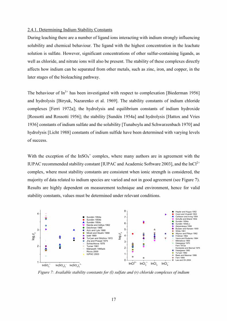
With the exception of the InSO4+ complex, where many authors are in agreement with the

IUPAC recommended stability constant [IUPAC and Academic Software 2003], and the InCl2+

complex, where most stability constants are consistent when ionic strength is considered, the

majority of data related to indium species are varied and not in good agreement (see Figure 7).

Results are highly dependent on measurement technique and environment, hence for valid

stability constants, values must be determined under relevant conditions.

1 2 31

2

3

4 Sundén 1954a Sundén 1954b Sundén 1954c Nanda and Aditya 1962 Deichman 1966 Aziz and Lyle 1968 Miceli and Stuehr 1968 Izatt 1969 Tur'yan and Strizhov 1972 Jha and Prasad 1975 Schischkova 1978 Turner 1981 Mahaseth 1995a/b Ricciu 2000 IUPAC 2003

log

x

InSO4+ In(SO4)2

– In(SO4)33–

1 2 3 4

0

1

2

3

4

5

6

7

8 Hepler and Hugus 1952 Cozzi and Vivarelli 1953 Carleson and Irving 1954 Schufle and Eiland 1954 Sundén 1954a Sundén 1954b,c Zelyanskaya 1958 Busaev and Kanaev 1959 White 1961 Altynov and Ptitsyn 1962 Fridman 1962 Vavra and Rudenko 1964 Mikhailova 1969 Hasegawa 1970 Ferri 1972a Kondyiela and Biernat 1975 Hasegawa 1980 Tur'yan 1982 Baes and Mesmer 1986 Ferri 1994 Lee and Oh 2004

log

x

InCl2+ InCl2+ InCl3 InCl4

–

Figure 7: Available stability constants for (l) sulfate and (r) chloride complexes of indium

18

The main focus of this work was to develop a quick, facile, and quantitative determination

method for the speciation and complexation constants of indium in process-relevant solutions.

2.4.2. Determining Leachate Composition

As previously mentioned, leaching solutions will contain a number of metal ions and

complexing ligands and the concentrations of these species must be determined for accurate

geochemical modelling. A fast, preferably in-situ, method is necessary for both separation and

quantification.

When analysing mixed metal solutions, one issue is the separation of components for

simultaneous analysis. Extensive broad-spectrum analysis methods can yield results with

overlapping or interrupted signals which introduces significant errors. Measurements with

procedures that differ between elements can be complex and time consuming. A simple,

simultaneous determination of metal ion concentrations in the leachate is required.

The biggest issue facing the analysis of sulfur species is the instability of intermediate

complexes. The analysis method must preserve speciation in the leachate rather than induce

decomposition of these compounds. Due to the leaching mechanism of sphalerite, the focus of

this work will be on the separation and quantification of the various polysulfide chains.

2.4.3. Geochemical Modelling of Process Solutions

Experimentally determined stability constants, component concentrations, and solution

parameters will be included in geochemical modelling software to determine indium behaviour

under the conditions of bioleaching and extraction, as well as with respect to certain parameters

such as pH or redox potential. It will be possible to observe how changing conditions such as

temperature, pH, and concentration can control solution behaviour. The ability to adjust indium

activity by modifying solution conditions, i.e. causing selective precipitation at a specific pH,

or minimising formation of complexes that interfere with solvent extraction, could result in

more efficient leaching and extraction processes.

19

3. Theoretical Background

The following section is a collection of the theoretical fundamentals relevant to this work.

Initially this focuses on equilibrium constants: their meaning, relevance, and methods of

determination. In the final parts of this section, the spectroscopic, electrochemical, and

chromatographic methods used in this work will be explained. For detailed experimental

procedures see Appendix i.

3.1. Equilibrium Constants

As the determination of stability constants will be a major component of this work, a brief

review of the fundamentals will be given here. The definitions of various equilibrium constants,

techniques to determine these values is also included.

An equilibrium constant is the reaction quotient of a chemical reaction at equilibrium [Ewing,

Lilley et al. 1994]. Constants are independent of analytical concentration but rely heavily on

temperature and ionic strength. The reaction quotient at equilibrium, Qeq, and therefore the

equilibrium constant, K, for a homogeneous reaction can be defined as:

𝛼A + 𝛽B ⇌ γC + δD 𝑄𝑒𝑞 = {C}𝛾{D}𝛿

{A}𝛼{B}𝛽= 𝐾 (26)

Quantities A, B, C, and D can be the equilibrium values of either pressure, fugacity,

concentration, or activity defining the pressure based, fugacity based, concentration based, or

standard equilibrium constant (Kϴ) respectively [IUPAC 2014].

3.1.1. Stepwise and Cumulative Stability Constants

A stability constant is an equilibrium constant for the formation of a complex. It is a measure

of the strength of the interaction between complex-forming reagents where a larger value

indicates a stronger complex. The formation of a metal-ligand complex in aqueous solutions

usually proceeds via a substitution reaction:

M(H2O)𝑥 + L ⇌ [M(H2O)𝑥−1L] + H2O (27)

20

The equilibrium constant for this reaction is expressed in equation 28. By assuming the activity

of water is constant, this equation can be simplified:

𝛽 = [M(H2O)𝑥−1L]

[M(H2O)𝑥][L] =

[ML]

[M][L] (28)

Stability constants for metal complexes, are generally expressed as association constants. A

cumulative association constant, β, is related to the direct formation of a complex from its

constituents. For the formation of a metal-ligand complex MLx, the cumulative constant is

defined as:

M + 𝑥 L ⇌ ML𝑥 𝛽𝑥 = [ML𝑥]

[M][L]𝑥 (29)

Whereas a series of stepwise association constants, K, for a complex, would be defined as:

M + L ⇌ ML𝑦 𝐾𝑦 = [ML𝑦]

[M][L] (30)

ML𝑦 + L ⇌ ML𝑦+1 𝐾𝑦+1 = [ML𝑦+1]

[ML𝑦][L] (31)

Where here y = 1. It follows that a cumulative constant is the product of its stepwise constants,

such that βx = Ky × Ky+1 × … Kx, and log βx = log Ky + log Ky+1 + … log Kx [Denbeigh 1981].

3.1.2. Hydrolysis Constants

When a metal ion forms a complex with a hydroxide ligand, an additional equilibrium must be

considered as formation of a hydrolysis complex of a metal ion can be expressed in two ways:

either by addition of a hydroxide ligand, or by deprotonation of an associated water molecule.

In aqueous solutions the concentrations of hydroxide ions and protons are related by the ionic

product of water, Kw = [H+][OH–], where at 25 °C –log Kw = 14.

M + OH− ⇌ M(OH) 𝐾 = [M(OH)]

[M][OH−] (32)

21

M(H2O) ⇌ M(OH) + H+ 𝛽 = [M(OH)]

[M][H+]−1= 𝐾 ∙ 𝐾𝑤 (33)

In general, when the hydrolysis product contains x hydroxide groups log β = log K + x log Kw,

which leads to them appearing to have unusually negative values.

3.1.3. Solubility Products

A solubility product Ksp is the equilibrium constant related to the dissolution of a solid phase

into an aqueous solution.

M(OH)𝑥 (s) ⇌ M𝑥 + 𝑥 OH− 𝐾sp = [M𝑥][OH−]𝑥 (34)

The solubility products of hydroxides can be given in a modified form, K*sp, defined as a

function of proton rather than hydroxide ion concentration [Baes and Mesmer 1976]. Similar

to hydrolysis constants, the two forms are related by the self-ionisation of water.

M(OH)𝑥 (s) + 𝑥 H+ ⇌ M𝑥 + 𝑥 H2O 𝐾sp∗ = [M𝑥][H+]−𝑥 =

𝐾sp

𝐾𝑤𝑥 (35)

These modified solubility products and hydrolysis constants are often used in geochemical

modelling software as pH, and hence proton concentration, is one of the required solution

parameter that must be defined by the user.

3.1.4. Thermodynamic Considerations

The link between stability and potential can be seen when considering Gibbs energy.

Equilibrium constants and potential, E, are related by the standard Gibbs free energy change,

ΔGϴ, which has contributions from enthalpy, ΔHϴ, and entropy, ΔSϴ:

∆𝐺Ѳ = −2.303 𝑅𝑇 log 𝐾 = −𝑛𝐹∆𝐸 = ∆𝐻Ѳ − 𝑇∆𝑆Ѳ (36)

Where R is the gas constant, T is temperature, n the stoichiometric number of electrons, and F

the Faraday constant. When both the standard enthalpy change (usually determined

calorimetrically) and stability constant are known, the standard entropy change is easily

calculated. The entropy factor can partly explain why stepwise stability constants of MLx

22

complexes usually decrease with increasing x. For the first ligand substitution, the ligand has a

choice of many water molecules to replace, as more ligands bind to the metal, available binding

sites become limited, hence disorder decreases with n. A more positive ΔS⊖ yields a more

negative ΔG⊖ and log K1 > log K2 [Beck and Nagypál 1990].

As previously stated, a standard equilibrium constant is a ratio of the thermodynamic activities

of products and reactants at equilibrium. A thermodynamic activity is the product of an analytes

concentration and activity coefficient, γ. To avoid complications using activities, stability

constants are determined in an inert electrolyte medium at high ionic strength, i.e. constant γ

even with slight variations in analyte concentration [Rossotti and Rossotti 1961]. Published

stability constants refer to the specific ionic medium used in their determination and different

values are obtained under different conditions. Often stability constants will be determined at

a range of ionic strengths, the values are then extrapolated to yield a stability constant at zero

ionic strength using specific ion interaction theory [Guggenheim and Turgeon 1955; Ciavatta

1990]. Hence it is always more desirable to determine a stability constant under the specific

conditions of interest.

Equilibrium constants also vary with temperature according to the Van’t Hoff equation, where

during an exothermic reaction (negative ΔH⊖), K decreases with temperature and the reverse

trend is observed for endothermic reactions [Atkins and Paula 2006].

𝑑(ln 𝐾)

𝑑𝑇=

∆𝐻𝜃

𝑅𝑇2 (37)

3.1.5. Previous Experimental Determination of Indium Stability Constants

An equilibrium constant can be expressed as a function of reactant and product concentration.

Hence, an equilibrium constant can be determined if these concentrations can be measured

[Schwarzenbach, Flaschka et al. 1969]. Typically, a titration is performed with one reactant in

the sample and another in the titrant. By knowing the initial concentrations, all analytical

concentrations can be derived as a function of the titrant volume added [Rossotti and Rossotti

1961].

The published stability constants of indium complexes originate from a variety of techniques.

Potentiometric methods are the most accurate for studying complexation of metal ions [Martell

23

and Motekaitis 1990; Janrao, Pathan et al. 2014] thus it has been the most commonly used

technique [Sundén 1954a; Aksel'rund and Spivakovskii 1959; Biederman, Li et al. 1961; Ferri

1972a, 1972b; Brown and Ellis 1982; Ferri, Salvatore et al. 1994; Mahaseth, Jha et al. 1994,

1995a, 1995b; Sundén 1953]. Most measurements have been carried out with quinhydrone or

indium amalgam electrodes, as producing a practical indium-selective electrode is challenging

due to the trivalent charge of the indium cation.

Constants have been determined from the analysis of indium absorption spectra [Biryuk,

Nazarenko et al. 1969; Tunaboylu and Schwarzenbach 1970; Nanda and Aditya 1962;

Rudolph, Fischer et al. 2004], however low intensity and significant spectral overlap makes

this a less than ideal technique. pH titration methods [Moeller 1942; Hepler and Hugus 1952;

Moeller 1941], calorimetrical methods [Izatt, Eatough et al. 1969], solubility measurements

[Deichman, Rodicheva et al. 1966], radioactive tracers [Rossotti and Rossotti 1956; Carleson

and Irving 1954], and ion exchangers [Sundén 1954b; Ferguson, Dobud et al. 1968; Schufle

and Eiland 1954; Schischkova 1978] have also been reported. 113In and 115In are both

quadrupolar and produce extremely broad lines, recent NMR analysis has yielded speciation

analysis [Deferm, Onghena et al. 2017] but not stability constants.

The two main experimental methods that have been previously applied to the determination of

indium stability constants are potentiometric and spectrophotometric titrations.

Potentiometric

Potentiometric measurements to determine complexation constants, such as those used by

[Sundén 1954c] and [Ferri 1972a] are based on the work of [Bjerrum 1941]. Assuming an

equilibrium constant βx, such as the one shown in equation 29, the total metal ion and total

ligand ion concentrations can be described by the following equations:

[In]𝑡𝑜𝑡 = [In3+]𝑓(1 + ∑ 𝛽𝑥[L−]𝑓𝑥)

𝑋

𝑥=1

[L]𝑡𝑜𝑡 = [L−]𝑓 + [In3+]𝑓 ∑ 𝑥𝛽𝑥[L−]𝑓𝑥

𝑋

𝑥=1

(38)

Where X is the maximum coordination number of the indium complex and [In3+]f and [L–]f are

the concentrations of the free indium and complexing ligand ions respectively. If the

1 + ∑ 𝛽𝑥[L−]𝑓𝑥𝑋

𝑥=1 term is called Z, the equations can be simplified:

24

[In]𝑡𝑜𝑡 = [In3+]𝑓𝑍 [L]𝑡𝑜𝑡 = [L−]𝑓 + [In3+]𝑓[L−]𝑓

𝑑𝑍

𝑑[L−]𝑓 (39)

It is possible to determine the polynomial Z through measurements of either [In]tot or [L]tot,

often called central ion or ligand measurements respectively. At constant [In]tot values, the

concentration of [L]tot is increased via titration and the potential, E’, of this solution measured.

Simultaneously a potential, E0, is measured in a solution under the same chemical conditions

but at [In]tot = 0. The difference between these potentials ΔE’ can be expressed as:

∆𝐸′ = 𝐸′ − 𝐸0 =2.303 𝑅𝑇

𝑛𝐹log

[In]𝑡𝑜𝑡

[In3+]𝑓 (40)

Using the relationship between [In]tot, [In3+]f, and Z as given in equation 39:

Δ𝐸’ =2.303 𝑅𝑇

𝑛𝐹log 𝑍 ∴ 1 + ∑ 𝛽𝑥[L−]𝑓

𝑥

𝑋

𝑥=1

= 10𝑛𝐹∆𝐸′

2.303 𝑅𝑇 (41)

In order to calculate βx and x from Z, the coordination number, x, and the free ligand

concentration [L–]f must be determined. A plot of [L]tot against [In]tot when considering ΔE’,

produces a series of linear fits where the gradient is equal to x. When these linear fits are

extrapolated to [In]tot = 0, it follows that [L–]f = [L]tot. The Z polynomial can be solved to yield

the stability constants of the complexes according to [Sundén 1953]:

𝑍𝑛 = (𝑍𝑛−1 − 𝛽𝑛−1)

[L−]𝑓= 𝛽1 + 𝛽2[L−]𝑓 + 𝛽3[L−]𝑓

2… (42)

A plot of Zx against [L–]f yields a curve with intercept βx. For example, Z1 is calculated from

the equation:

𝑍1 = (𝑍0 − 𝛽0)

[L−]𝑓 (43)

Where Z is calculated from equation 41, β0 is unity, and [L–]f is known. A plot of Z1 against

[L–]f, extrapolated to [L–]f = 0 yields the value β1. The plot for the last complex formed

25

(maximum coordination number, X) will be a straight line parallel to the x axis. The plot for

the penultimate complex will be a straight line with a positive gradient and all previous plots

will be curved. Alternatively, βx can be determined numerically from a series of simultaneous

equations for Z and [L–]f [Heath and Hefter 1977].

While this is a well-established method, accuracy depends heavily on the ΔE’ term, i.e. the two

simultaneous titrations must be extremely accurate. Furthermore, data analysis is extensive and

complicated with a multiple graphical analysis required for each stability constant.

Potentiometry is the measurement of a potential between two electrodes in a solution. One

electrode is a reference with a stable potential, while the potential of the other electrode varies

with sample composition. Later in this work (section 3.4) a voltammetric measurement

procedure is introduced where a potential is applied at an electrode surface and the resulting

current is measured with a three electrode system. Although the voltammetric method is not

too dissimilar to the measurement principle discussed here, measurements are fast, precise, and

simpler to analyse.

Spectrophotometric

In most spectroscopic determination of equilibrium constants, the concentration of a coloured

metal complex can be determined using the Beer-Lambert law [Spencer 1973], which describes

the linear relationship between the absorbance of a species and its concentration, c, molar

absorption coefficient, ε, and path length of light through the sample, l:

𝐴𝑏𝑠 = 휀𝑐𝑙 (44)

However, In3+ salt solutions are colourless so using direct spectroscopic methods in the visible

region is not possible. A common alternative to direct methods is the use of competing

complexes, i.e. copper sulfate gives a strong absorbance signal at around 800 nm [Inoue,

Philipsen et al. 2012], addition of In(ClO4)3 results in a significant decrease in this signal

implying formation of InSO4+, the stability of this complex can be calculated from the change

in signal and the known stability of CuSO4 [Nanda and Aditya 1962]. Alternatively a

competing ligand approach can be used, where the alternative ligand usually forms an intensely

coloured complex i.e. an indicator [Biryuk, Nazarenko et al. 1969].

26

Precise spectroscopic measurements usually have an upper limit of log β = 4 due to the

detection limits of the spectrometer. A significant disadvantage of spectroscopic measurements

arises during investigations of more complex systems when interference can occur between

overlapping spectra of multiple species.

3.1.6. Computational Determination of Stability Constants

As well as experimental methods, there are also computational methods available for the

determination of stability constants [Deelstra, Vanderleen et al. 1963; Paoletti, Vacca et al.

1966]. In general, a computational procedure consists of three stages: definition of the chemical

model, calculation of speciation and concentrations, and further refinement of equilibrium

constants [Leggett 1985].

A chemical model defines a set of chemical species in solution, as well as the solution

properties. A model is constrained by the laws of mass action and mass balance. Complexes

are defined stoichiometrically by the combination of reactants forming them. In dilute solutions

the concentration of water is assumed constant, and for simplicity inert species (supporting

electrolytes), or species at very low concentrations are omitted from the model.

A speciation calculation is made by calculating the concentrations of all species in an

equilibrium. This requires solving a series of non-linear mass balance equations such as the

ones in equation 38. Free reactant concentrations (e.g. [In3+]f or [L–]f) are initially estimated

but are then refined using methods such as Newton-Raphson iterations [Marinoni, Carrayrou

et al. 2017; I and Nancollas 2002; Crerar 1975]. From the free reactant concentrations and

estimated equilibrium constants, concentrations of the complexes can be derived.

Initially equilibrium constants are usually estimated from literature data sources. The aim of a

refinement process is to determine an equilibrium constant that gives the best fit to a set of

experimental data. This is usually achieved by minimising a function using a non-linear least-

squares method such as the Gauss-Newton algorithm [Leggett 1985; Potvin 1990]. A number

of computer programs exist for the calculation of equilibrium constants. For potentiometric

data the most common programs are Hyperquad [Gans, Sabatini et al. 1996], BEST [Martell

and Motekaitis 1992], and PSEQUAD [Zekany and Nagypal 1985]. For spectroscopic data

HypSpec, SQUAD, and Specfit [Gampp, Maeder et al. 1985] are frequently used.

27

In the scope of this research it was necessary to develop a quick, facile, and quantitative

determination method for the speciation and complexation constants of indium in process-

relevant solutions. Both voltammetric and spectroscopic techniques were investigated to

characterise indium behaviour in solution. Eventually a polarographic technique was

developed to simultaneously yield speciation and stability. The fundamentals of these

experimental measurements are discussed in the following sections.

3.2. Spectroscopic and Electrochemical Experimental Techniques

To characterise aqueous solutions of indium, specifically the interaction of indium with various

ligand anions, spectroscopic (Ultraviolet–visible spectroscopy, Extended X-Ray Absorption

Fine Structure) and electrochemical (voltammetry, quartz crystal microbalance) measurements

were made. Experimental details regarding these measurements can be found in Appendix i.

3.2.1. Ultraviolet–Visible Spectroscopy

Ultraviolet–visible (UV-Vis) spectroscopy refers to absorption spectroscopy in the UV and

visible electromagnetic spectral regions, where atoms and molecules undergo electronic

transitions from ground to excited states [Skoog, Holler et al. 2008]. The total potential energy

of a molecule is a sum of its electronic, vibrational, and rotational energies. Electronic energy

levels of simple molecules are widely spaced and usually only the absorption of a high energy

photon can excite a molecule. In complex molecules energy levels are more closely packed and

photons of near-ultraviolet and visible light can induce transitions [Kaufmann 2003].

When light passes through a sample, the absorbed light is the difference between the incident

and transmitted radiation. This can be expressed as transmittance but more commonly as

absorbance (the reciprocal of transmittance) due to the linear relationship between absorbance

and both concentration and path length, described by the Beer-Lambert law (equation 44).

Frequently UV-Vis spectra show multiple broad absorption bands. Compared with techniques

such as IR spectroscopy, UV-Vis spectroscopy can provide a limited amount of qualitative

information. However, if there are suitable characteristic peaks, it is still possible to yield

concentration (calibration curves using the Beer-Lambert law), the stoichiometry of metal-

ligand complexes (method of continuous variations), and equilibrium constants. UV-Vis

methods are most applicable to transition metal complexes or highly conjugated organic

compounds due to the excitement of d- and π-electrons respectively [Misra and Dubinskii

2002].

28

3.2.2. Extended X-Ray Absorption Fine Structure

X-ray Absorption Spectroscopy (XAS) includes both Extended X-Ray Absorption Fine

Structure (EXAFS) and X-ray Absorption Near-Edge Structure (XANES). X-rays of a narrow

bandwidth are shone through a sample and the increasing incident, and resultant transmitted

x-ray intensities are recorded. The number of x-ray photons transmitted through a sample, It, is

equal to the product of the incident photons, I0, and a decreasing exponential which depends

on the atoms in the sample, the absorption coefficient, µ, and the sample path length, χ. The

absorption coefficient can be obtained from the logarithmic ratio of the incident, I0, and

transmitted, It, x-ray intensities (an alternative form of the Beer-Lambert) [Stern 2001].

µ =ln (

𝐼𝑡

𝐼0)

𝜒

(45)

When the incident photon energy is equivalent to the binding energy of an electron of an atom

in the sample, the number of x-rays absorbed by the sample dramatically increases, resulting

in an absorption edge. Absorption edges are unique for all elements, corresponding to different

binding energies of electrons, giving XAS elemental selectivity as well as the ability to focus

on specific elements of interest [Rehr and Albers 2000]. Absorption results in the emission of

a wave-like photoelectron, interference caused by the scattering of this wave off surrounding

atoms results in an oscillation in the absorption coefficient with increasing energy. The

amplitude of the backscattered wave is proportional to the scattering strength of the

backscattering atom, which is related to electron density. The phase of the wave is correlated

to the distance of the backscattering atom from the central absorbing atom. From this EXAFS

interference pattern, the arrangement of atoms surrounding the absorbing central atom can be

determined [Groot 2001]. XAS is recorded as a plot of the absorption coefficient of the sample

against energy (Figure 8 (l)). A Fourier transform of the normalised, background subtracted

EXAFS region will give a plot of electron density as a function of distance from the central

absorbing atom (Figure 8 (r)).

31

In a reversible redox couple, the anodic and cathodic peak currents are equal and ipc/ipa = 1.

The Randles-Sevčik equation describes peak current [Matsuda and Ayabe 1955], at 25 °C it

can be expressed as:

|𝑖𝑝| = 2.687 × 105 𝐴𝑐√𝑛3𝐷𝑣 (48)

Where |ip| is the absolute peak current (A), A the electrode area (cm2), c the concentration

(mol cm–3), n the stoichiometric number of electrons, D the diffusion coefficient (cm2 s−1), and

v the scan rate (V s−1). Thus, peak currents are proportional to the concentration of the

electroactive species, as well as √𝑣. A plot of ip against √𝑣 is a good test of reversibility, it

should be linear and pass through the origin [Greef, Peat et al. 1985].

When initially only the oxidised species, Ox, is present in solution, a half wave reduction

potential, E1/2, for the reaction Ox + e– ⇌ Red, can be determined from the peak potentials:

𝐸12

= 𝐸𝑝𝑎 + 𝐸𝑝𝑐

2

(49)

For a reversible couple, the difference between the cathodic and anodic peak potentials should

equal 57.0/n mV.

With the electrochemical modelling software DigiElch [Bott, Feldberg et al. 1996], it is

possible to determine various thermodynamic and kinetic parameters in an electrochemical

reaction. The standard fitting protocol can be separated into three general stages:

1. Selection of experimental data

2. Suggest mechanism and input estimated chemical and electrochemical parameters

3. Select parameters to be fitted and run fitting software

Along with a suggested redox mechanism (i.e. In3+ + 3 e– ⇌ In), the number of electrons

consumed in the electrode reaction, an estimated standard reduction potential, and an electrode

area must be defined by the user. DigiElch produces a simulated CV curve which is then

compared to measured data, the standard deviation between these two curves is minimised

using an iterative Gauss-Newton method [Leggett 1985; Potvin 1990], similar to the

32

computational determination of stability constants (section 3.1.6). A number of parameters can

be optimised with DigiElch (redox potentials, electron transfer kinetic parameters, chemical

reaction rate constants, and diffusion coefficients). Unfortunately, as this number increases, so

does computational time, furthermore the possibility of finding a minimum in the error plot

decreases. Hence it is not recommended to use DigiElch to optimise all parameters

simultaneously. Additionally, while critically analysing a resulting fit, it is important to

consider that several mechanisms and parameter sets can be in good agreement with the

experimental data. In this work, the following parameters were calculated to analyse the

reversibility of an electrode reaction: the standard reduction potential, the rate constant of the

electrode reaction, and the transfer coefficient, α.

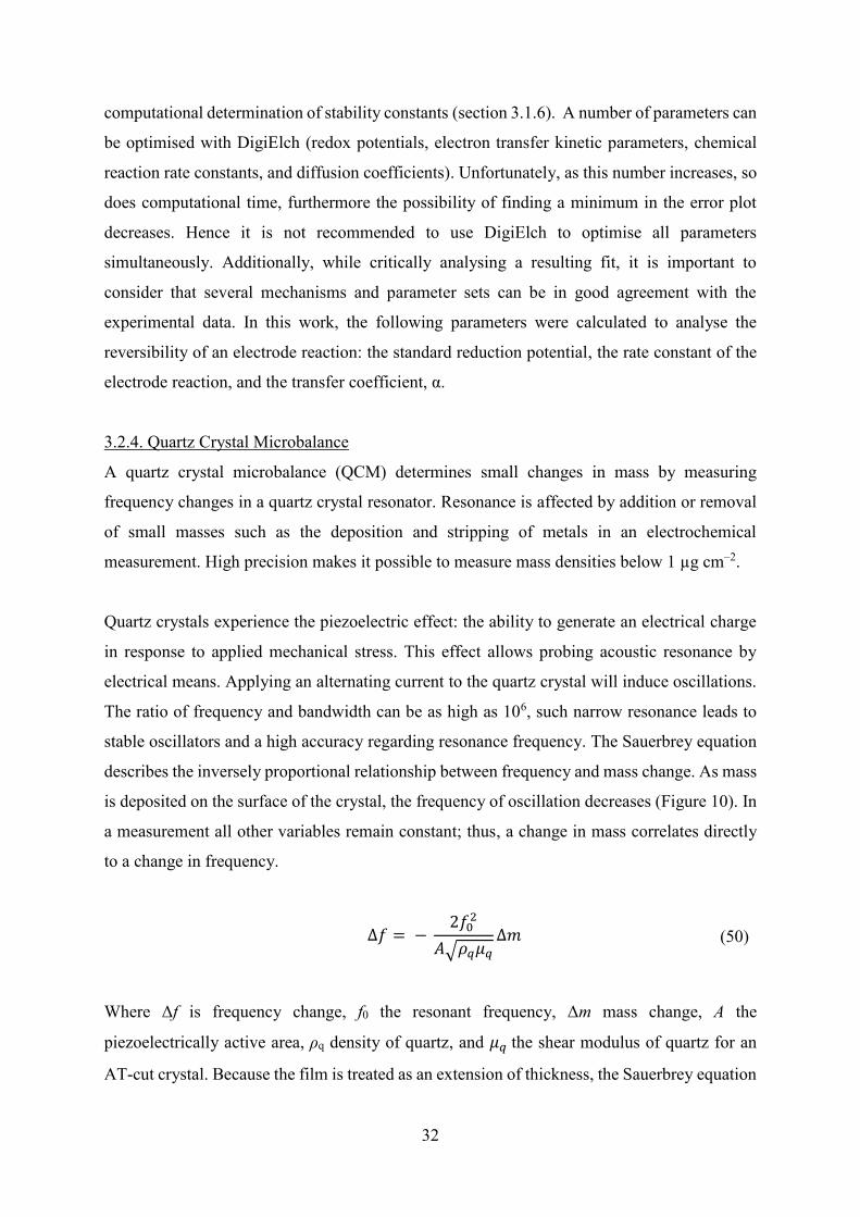
3.2.4. Quartz Crystal Microbalance

A quartz crystal microbalance (QCM) determines small changes in mass by measuring

frequency changes in a quartz crystal resonator. Resonance is affected by addition or removal

of small masses such as the deposition and stripping of metals in an electrochemical

measurement. High precision makes it possible to measure mass densities below 1 µg cm–2.

Quartz crystals experience the piezoelectric effect: the ability to generate an electrical charge

in response to applied mechanical stress. This effect allows probing acoustic resonance by

electrical means. Applying an alternating current to the quartz crystal will induce oscillations.

The ratio of frequency and bandwidth can be as high as 106, such narrow resonance leads to

stable oscillators and a high accuracy regarding resonance frequency. The Sauerbrey equation

describes the inversely proportional relationship between frequency and mass change. As mass

is deposited on the surface of the crystal, the frequency of oscillation decreases (Figure 10). In

a measurement all other variables remain constant; thus, a change in mass correlates directly

to a change in frequency.

∆𝑓 = − 2𝑓0

2

𝐴√𝜌𝑞𝜇𝑞

∆𝑚 (50)

Where Δf is frequency change, f0 the resonant frequency, Δm mass change, A the

piezoelectrically active area, ρq density of quartz, and 𝜇𝑞 the shear modulus of quartz for an

AT-cut crystal. Because the film is treated as an extension of thickness, the Sauerbrey equation

34

Figure 11: Schematic of (l) a mercury electrode and (r) a typical 3-electrode polarographic

measurement set-up (CE = counter electrode, WE = Hg working electrode, RE = reference electrode)

Similarly to traditional voltammetry, in polarography a potential sweep is applied to a working

electrode and the resultant current is recorded. When using a mercury electrode in HMDE

mode, a polarographic measurement produces a current signal analogous to a traditional

voltammogram. However, when measurements are performed on a DME or SMDE, although

measurements take place in a stagnant solution, the separation of the mercury drop from the

capillary disturbs the sample ensuring that each new drop grows into bulk solution. The

resulting signal (often called a polarographic wave) reaches a limited rather than peak current

(see Figure 12 (l)). The potential at the half height of this wave (ilim/2) corresponds to the half

wave reduction potential E1/2 [Kolthoff and Lingane 1939].

Mercury has several advantages as a working electrode. Its high overpotential for the reduction

of water to hydrogen can allow measurements at potentials as negative as –2 V (vs AgCl/Ag),

dependant on solution composition [Furman and Cooper 1950]. Metal deposition on other

electrode surfaces such as glassy carbon is often inhibited by electrocrystallisation kinetics and

can then be disrupted by simultaneous solvent breakdown (hydrogen evolution). In these cases,

it becomes impossible to distinguish between the currents relating to the reduction of analyte

and water. With a mercury electrode, most reduced metals form amalgams where often these

issues do not occur. Another advantage, specifically regarding the DME and SMDE, is by

replacing the drop at each measurement point, issues related to electrode surface fouling are

removed.

Due to its oxidation potential, the potential window of the mercury electrode is limited with

respect to positive potentials, depending on the solvent, mercury electrodes can be unusable

35

above 0.2 V (vs AgCl/Ag) [Bertram 1969]. In classical polarography for quantitative analytical

measurements, the current is continuously measured during the growth of the Hg drop,

therefore there is a substantial contribution from non-faradaic current. As the Hg flows from

the end of the capillary, initially there is a large increase in the surface area. As a consequence,

the initial current is dominated by capacitive effects, although this can be corrected for

measuring a background or residual current [Brett and Brett 1994]. Residual current has two

sources. One source is non-faradaic currents that accompanies a change in the working

electrode’s potential, which can be minimised using pulsed methods (see section 3.4). The

other source is faradaic currents from the oxidation or reduction of trace impurities in the

sample. Faradaic current due to impurities can be minimised by careful sample preparation,

e.g. using very pure chemicals, and by the removal of dissolved O2, which on a mercury

electrode undergoes a two-step reduction [Kolthoff and Lingane 1939]:

O2 + 2 H+ + 2 e− ⇌ H2O2 𝐸 ≈ −0.1 𝑉

H2O2 + 2 H+ + 2 e− ⇌ 2 H2O 𝐸 ≈ −0.9 𝑉

(52)

(53)

3.3.1. Determining Concentrations and Half Wave Reduction Potentials, E1/2

The Nernst equation for a simple reduction reaction is described below:

Ox + e− ⇌ Red 𝐸 = 𝐸𝜃 − 2.303 𝑅𝑇

𝑛𝐹log

[Red]

[Ox] (54)

To determine standard redox potentials from a polarographic wave, the Nernst equation must

be rewritten in terms of current instead of the concentrations. The current related to the

reduction of Ox depends on the rate at which it diffuses through the diffusion layer, δ. While

under diffusion control, the current, i, is equal to [Brett and Brett 1994]:

𝑖 = 𝑛𝐹𝐴𝐷(𝑐𝑏𝑢𝑙𝑘 − 𝑐𝑠𝑢𝑟𝑓)

𝛿 (55)

Where n the stoichiometric number of electrons, F the Faraday constant, A is electrode area, D

the diffusion coefficient, and cbulk and csurf are analyte concentrations in the bulk solution and

at the electrode surface respectively. Under the assumption that the only species present in the

bulk solution is Ox, the current from the reduction reaction equals:

36

𝑖 = 𝜎𝑂𝑥([Ox]𝑏𝑢𝑙𝑘 − [Ox]𝑠𝑢𝑟𝑓) (56)

Where σOx is a constant equal to nFADOx/δ. As limiting current, ilim, is reached the concentration

of Ox at the electrode surface approaches zero and equation 56 can be simplified to:

𝑖𝑙𝑖𝑚 = 𝜎𝑂𝑥 ∙ [Ox]𝑏𝑢𝑙𝑘 (57)

Hence limiting current is a linear function of [Ox] and polarography can be used to determine

analyte concentration. Typical signal to noise ratio allows detection limits of approximately

10−5 or 10−6 mol kg−1. The relationship between analyte concentration and the limiting current

is given by the Ilkovič equation [Bard and Faulkner 1980], derived from the Cottrell equation

for a planar electrode (equation 47):

|𝑖lim| = 708 𝑛 𝑐 √𝐷 √𝑚𝐻𝑔3 𝑡

16 (58)

Where |ilim| is the absolute limiting current (A), n is the stoichiometric number of electrons, c

is concentration (mol cm–3), D is the diffusion coefficient (cm2 s–1), mHg is the flow rate of

mercury (mg s–1), and t is the drop lifetime (s).

Equations 56 and 57 can be rearranged to give a term for [Ox]surf. From the assumption that the

only species in solution is Ox, the concentration of [Red]bulk is zero, and hence a similar

procedure can be followed to produce an equation for [Red]surf:

[Ox]𝑠𝑢𝑟𝑓 = 𝑖𝑙𝑖𝑚 − 𝑖

σ𝑂𝑥 [Red]𝑠𝑢𝑟𝑓 =

𝑖

σ𝑂𝑥 (59)

Substitution of equations 59 into the Nernst equation (equation 54) gives:

𝐸 = 𝐸𝜃 − 2.303 𝑅𝑇

𝑛𝐹log

σ𝑂𝑥

σ𝑅𝑒𝑑−

2.303 𝑅𝑇

𝑛𝐹log

𝑖

𝑖𝑙𝑖𝑚 − 𝑖 (60)

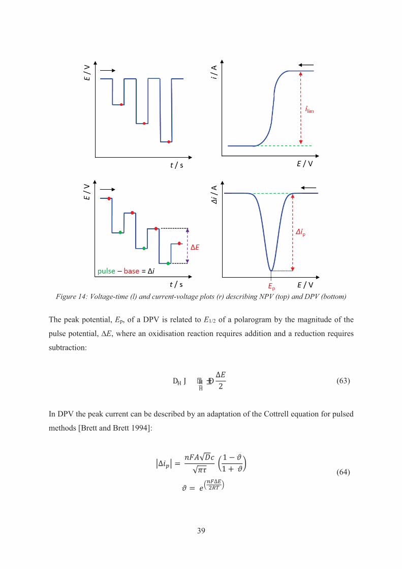
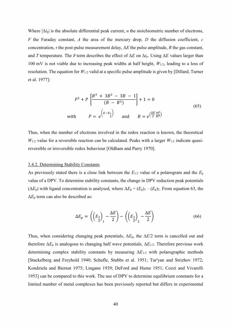
40

Where |Δip| is the absolute differential peak current, n the stoichiometric number of electrons,

F the Faraday constant, A the area of the mercury drop, D the diffusion coefficient, c

concentration, τ the post-pulse measurement delay, ΔE the pulse amplitude, R the gas constant,

and T temperature. The ϑ term describes the effect of ΔE on Δip. Using ΔE values larger than

100 mV is not viable due to increasing peak widths at half height, W1/2, leading to a loss of

resolution. The equation for W1/2 valid at a specific pulse amplitude is given by [Dillard, Turner

et al. 1977]:

𝑃2 + 𝑃 [

𝐵3 + 3𝐵2 − 3𝐵 − 1

(𝐵 − 𝐵2)] + 1 = 0

with 𝑃 = 𝑒(𝐸−𝐸1

2

) and 𝐵 = 𝑒(

∆𝐸2

𝑛𝐹𝑅𝑇

)

(65)

Thus, when the number of electrons involved in the redox reaction is known, the theoretical

W1/2 value for a reversible reaction can be calculated. Peaks with a larger W1/2 indicate quasi-

reversible or irreversible redox behaviour [Oldham and Parry 1970].

3.4.2. Determining Stability Constants

As previously stated there is a close link between the E1/2 value of a polarogram and the Ep

value of a DPV. To determine stability constants, the change in DPV reduction peak potentials

(ΔEp) with ligand concentration is analysed, where ΔEp = (Ep)1 – (Ep)2. From equation 63, the

ΔEp term can also be described as:

∆𝐸𝑝 = ((𝐸12

)1

−∆𝐸

2) − ((𝐸1

2)

2

−∆𝐸

2) (66)

Thus, when considering changing peak potentials, ΔEp, the ∆E/2 term is cancelled out and

therefore ΔEp is analogous to changing half wave potentials, ΔE1/2. Therefore previous work

determining complex stability constants by measuring ΔE1/2 with polarographic methods

[Stackelberg and Freyhold 1940; Schufle, Stubbs et al. 1951; Tur'yan and Strizhov 1972;

Kondziela and Biernat 1975; Lingane 1939; DeFord and Hume 1951; Cozzi and Vivarelli

1953] can be compared to this work. The use of DPV to determine equilibrium constants for a

limited number of metal complexes has been previously reported but differs in experimental

41

technique [Heath and Hefter 1977]. For simplicity, henceforth E1/2 rather than Ep will be used

to describe DPV peak potentials.

The complexation of the electrochemically active metal correlates with a shift in the E1/2 value.

For the reduction of an oxidised species, Ox, to reduced species, Red, the introduction of a

complexing ligand, L, leads to the reaction:

OxL𝑥 ⇌ Ox + 𝑥 L (67)

Because of its increased stability, reduction of the OxLx complex should be less favourable

than the reduction of Ox and hence occur at a more negative potential. This shift in potential

depends on the ligand concentration and x number of ligands bound to the metal. Therefore the

change in E1/2 with respect to ligand concentration is indicative of both the stoichiometry and

formation constant of a metal-ligand complex. A relationship between the relevant variables

can be constructed from two simple equations: the Nernst equation for the reduction of Ox

(equation 54) and the cumulative stability constant, βx, related to the formation of the metal

complex, OxLx (analogous to the stability constant for MLx in equation 29).

For a reversible redox couple, the half wave potential E1/2 is the potential at which exactly half

of the analyte close to the electrode surface has been reduced, i.e. when [Red]surf = [OxLx]surf.

When a ligand is present, its diminishing effect on the concentration of Ox must be considered.

Solving the stability constant term for [Ox] (equation 29) and substituting into the Nernst

equation gives:

𝐸 = 𝐸𝜃 − 2.303 𝑅𝑇

𝑛𝐹log

[Red][L]𝑥 𝛽𝑥

[OxL𝑥]

(68)

If the stability constant is sufficiently large that a strong complex is formed, essentially all [Ox]

is bound in a complex. This means that at E1/2 [Red] and [OxLx] are equal and equation 68 can

be simplified:

(𝐸12

)𝑐𝑜𝑚 = (𝐸12

)𝑓 − 2.303 𝑅𝑇

𝑛𝐹log([L]

𝑥𝛽𝑥)

(69)

42

Where the subscripts ‘com’ and ‘f’ indicate ‘complexed’ and ‘free’ metal ions respectively and

therefore Eϴ = (E1/2)f. When ∆E1/2 is the difference between (E1/2)com and (E1/2)f, equation 69

can be rearranged to give:

∆𝐸12

= − 2.303 𝑅𝑇

𝑛𝐹log 𝛽𝑥 −

2.303 𝑅𝑇𝑥

𝑛𝐹log [L]

(70)

Therefore, plotting ∆E1/2 against log [L] would produce a linear plot, where x can be obtained

from the gradient and log βx from the y-axis intercept. In summary, a simple measurement of

E1/2 as a function of ligand concentration can yield both the speciation and stability constant of

a metal complex. However, it is essential to maintain both metal ion concentration and ionic

strength during one series of measurements.

A notable advantage of DPV over cyclic voltammetry in determining E1/2 values specifically

for these measurements, is the opportunity to determine the speciation of indium in-situ in

leachate samples containing other redox-active ions. Due to sufficiently different redox

potentials of couples such as Fe3+/0, Cu2+/0, Zn2+/0, and In3+/0 (see Table 3), it may also be

possible to determine the speciation and stability of a range of metal ions found in the leachate

simultaneously.

-1.0 -0.8 -0.6 -0.4 -0.2 0.0 0.2

-3.5

-3.0

-2.5

-2.0

-1.5

-1.0

-0.5

0.0

Ni2+/0

Ep = –1.031 V

Pb2+/0

Ep = –0.363 V

Cr3+/0

Ep = –0.836 VIn3+/0

Ep = –0.489 V

Cd2+/0

Ep = –0.560 V

Zn2+/0

Ep = –0.983 V

i /

A

E / V

Cu2+/0

Ep = 0.042 V

no peaks: Mn2+/0, Fe3+/2+/0, Co2+/0

Figure 15: DPV measurements of 100 mg L−1 standard solutions of common leachate components

Figure 15 shows the DPV reduction peaks from standard solutions of metal ions commonly

found in the leachate. While it was not possible to produce peaks for all common leachate

components, e.g. Fe3+/0 which was outside the potential window of mercury, or Mn2+/0 where

43

reduction was not observed on the HMDE, a number of elements could be qualified using this

method. Issues may arise with the simultaneous determination of nickel and zinc, or cadmium

and indium, where peaks are not well separated. In these measurements all standard solution

concentrations were 100 mg L−1, however the sensitivity of DPV would allow measurement of

highly dilute samples, additionally investigation of a specific metal ion next to a large excess

of other elements, i.e. under similar conditions to that of indium in the leachate.

The E1/2 values calculated from the DPV peak potentials are listed in Table 3. The values are

in good agreement with the standard reduction potentials when the reference potential is taken

into consideration. The reduction of nickel on the mercury drop electrode occurs at a

significantly more negative potential than the standard redox potential. This is consistent with

measurements by [Torrance and Gatford 1985; Pihlar, Valenta et al. 1981; Flora and Nieboer

2002]. The likely cause of this phenomenon is formation of solid nickel in the HMDE amalgam.

A mixed phase containing solid nickel can be seen even at low nickel atomic percentages in a

mercury-nickel phase diagram [Massalski 2007], whereas most other metals form a liquid

amalgam under similar conditions.

Table 3: Standard redox potentials of leachate metal ions, Eϴ vs Ag/AgCl 3 mol kg−1 KCl (195 mV vs SHE), [Bard and Parsons 1985] and measured E1/2 values calculated from the Ep of a DPV

Eϴ / V E1/2 / V

Fe3+/2+ 0.576 -

Cu2+/0 0.145 0.055

Fe3+/0 –0.231 -

Pb2+/0 –0.320 –0.351

Ni2+/0 –0.452 –1.019

In3+/0 –0.533 –0.477

Cd2+/0 –0.598 –0.546

Fe2+/0 –0.635 -

Cr3+/0 –0.939 –0.824

Zn2+/0 –0.958 –0.983

3.5. Techniques to Determine Diffusion Coefficients

For members of the BHMZ who are investigating selective filtration as a method to extract

indium from leachate solutions, the diffusion coefficients of In3+ and relevant indium

44

complexes are important parameters. Diffusion coefficients can be used to calculate

hydrodynamic radii which are essential for selection of membranes with valid pore sizes. A

number of electrochemical methods were employed to determine the diffusion coefficients of

some indium species.

As previously mentioned, current measured during dynamic electrochemical experiments can

be divided into two parts: current under electron transfer kinetic control and under mass

transport control. Mass transport of an analyte is defined by the Nernst-Planck equation:

𝐽(𝑙) = −𝐷𝜕𝑐(𝑙)

𝜕𝑙+

−𝑧𝐹

𝑅𝑇𝐷𝑐

𝜕∅(𝑙)

𝜕𝑙+ 𝑐𝑣(𝑙) (71)

Where J(l) is the flux of the electroactive species at a distance l from the electrode surface, D

is the diffusion coefficient, ∂c(l)/∂l is the concentration gradient, ∂∅(l)/∂l is the potential

gradient, z and c are the charge and concentration respectively, v(l) is the velocity, F and R are

the Faraday and gas constants and T is temperature. The three terms represent the contributions

of diffusion, migration and convection to the flux of the electroactive species.

Electrochemical analysis techniques for the determination of diffusion coefficients are

designed such that diffusion is the only source of mass transport. If a measurement is conducted

in a stagnant solution containing an inert supporting electrolyte of suitable concentration,

migration and convection can be neglected. The diffusion coefficient is simply the

proportionality between flux, J(l), and the concentration gradient, ∂c(l)/∂l, as expressed in

Fick’s first law:

𝐽(𝑙) = −𝐷𝜕𝑐(𝑙)

𝜕𝑙 (72)

Faradaic currents are proportional to flux at the electrode surface, J0:

𝑖 = −𝑛𝐹𝐴𝐽0 (73)

Hence, in a redox reaction where the stoichiometric number of electrons and the electrode area

are known, voltammetric measurements are a simple technique to determine diffusion

coefficients.

46

t time, and r0 is electrode radius. The diffusion coefficient can be calculated from the gradient

of a linear plot of |id| against 1/√𝑡.

Cyclic and Differential Pulse Voltammetry

The fundamentals of cyclic voltammetry have already been discussed in section 3.2.3 and will

not be repeated. The peak current, ip, of a voltammogram is related to the diffusion coefficient

by the Randles-Sevčik equation (equation 48).

An adaptation of the Cottrell equation (described in equation 64) can be used to determine

diffusion coefficients from differential currents in pulsed voltammetric methods.

3.6. Geochemical Modelling

A geochemical model is a tool to calculate complex chemical reactions and equilibria in natural

systems. A model is defined with certain constraints e.g. the laws of mass action and mass

balance, so equilibrium constants for reactions in the overall composition are chemically valid.

A model should never be so simplified that it is unrealistic nor so detailed it cannot be

accurately calculated. Geochemical modelling is widely used in environmental protection and

remediation [Zhu and Anderson 2002], specifically predicting mobility and stability of

contaminants in groundwater, generation of acidic waters, or leaching of metals from mine

waste. In economic geology the dissolution of minerals in response to industrial wastes, waters,

or gases can be modelled [Bethke 2008]. In this study the overall aim is to use geochemical

modelling to predict the behaviour of target metals in complex process relevant solutions such

as leachate and extraction solutions.

3.6.1. Defining a Geochemical Model

To create a geochemical model, concentrations of the aqueous species, minerals, and gases

present in the system (the basis) must be defined, as well as chemical conditions such as pH,

temperature, and redox potential. Analogous to pH, in most modelling programs the redox

potential is defined by the function ‘pe’, where pe is the negative logarithm of electron activity.

The relationship between redox potential, E, and pe is –log{e–}a = 16.9 × E.

Typically, the basis is composed of water, elements, minerals, and gases. Once the basis is

defined, a modelling program can calculate the equilibrium state of species distribution,

47

mineral saturation indicies, and gas fugacities. The saturation index (SI) describes the equilibria

of solid phases, typically when a phase has a SI between –1 and 1, the mineral is considered to

be at equilibrium, a more negative SI indicates a soluble phase, and a positive SI indicates

precipitation. Typically geochemical models define all chemical equations in terms of a master

species, then iteratively refines the values of the master unknowns (unknowns for species i, are

activity, ai, the activity coefficient, γi, molality, mi, and amount in solution, ni) until the

convergence criteria for the set of simultaneous equations is met. For aqueous species to be at

equilibrium in an ion-association model, all mass-action equations must be satisfied.

A geochemical modelling program generally involves three datasets, the database, the input,

and the output files. The database contains definitions of possible chemical species, phases,

and gasses, and is a collection of their respective thermodynamic constants. An input file is

written by the user to produce the model. Basis composition and properties, any reactions that

are occurring, and desired data output are specified in the input file. An output is the results of

the calculations carried out by the program which should always be critically evaluated.

Geochemical modelling programs are essentially calculators and hence the accuracy of results

entirely depends on the validity of the input and database files.

Geochemical models are capable of simulating multiple reactions and processes including:

acid-base and redox reactions, complexation, mineral dissolution and precipitation, ion-

exchange, and radioactive decay. Commonly speciation, batch reaction, transport, or inverse

modelling are employed [Bethke 2008]:

1. Speciation Modelling – useful for predicting aqueous species distribution as well as

mineral dissolution or precipitation e.g. modelling of waste water treatment.

2. Batch Reaction Modelling – can be divided into equilibrium reactions (equilibria

between solutions, minerals, or gas phases) and non-equilibrium reactions (kinetic

reactions, addition or removal of elements, mixing, or temperature change). Used

frequently in the study of mine drainage and radioactive waste disposal.

3. Transport Modelling – can be used to study contaminant migration, diffusion in

sediments, and chemical evolution of natural systems. It can simulate diffusion,

dispersion, or chemical reactions as water moves through a one-dimensional column

when a column is divided into a series of finite defined cells.

4. Inverse Modelling – can be used to deduce previous geochemical reactions along a flow

path that resulted in a final defined model composition. At least two chemical analyses

48

of the solution at different points along the flow path are required. Phases are calculated

that account for changes in water composition between these points.

3.6.2. PHREEQC

While many modelling programs exist, PHREEQC (pH-REdox-EQuilibrium) a freely

available geochemical modelling program written in the C++ programming language, was

selected for this work [Parkhurst and Appelo 2013]. It can be used to calculate the distribution

of species in a specified solution. For calculating solute activities, PHREEQC uses ion-

association, Pitzer [Pitzer 1991], or specific ion interaction theory (SIT) equations

[Guggenheim and Turgeon 1955] to account for the non-ideality of aqueous solutions.

Distribution of elements among stable valence states can be observed based on a defined redox

potential which is key when modelling redox active solutions such as ferric and ferrous iron

containing leachates.

One limitation of the program, specifically in aqueous speciation modelling, is the lack of

consistency in the databases supplied by PHREEQC. The databases are a collection of

equilibrium constants taken from a variety of literature sources and only for a limited number

of elements. No systematic analysis of the quality of these values has been carried out and the

databases provided should be considered ‘preliminary’. Hence, careful selection of aqueous

species and thermodynamic data is the responsibility of the user. While thermodynamic

constants related to the more common components of the leachate (e.g. iron, zinc, copper, and

sulfur) were included in the databases supplied by PHREEQC, equilibrium constants of indium

complexes were not. In order to model speciation of indium under the conditions of

bioleaching, the stability constants determined by DPV methods would have to be added to the

database. In addition, ionic strengths used in stability constant determination are much higher

than the limits of the Debye–Hückel expressions considered by PHREEQC [Debye and Hückel

1923]. In an attempt to minimise inaccuracies, an equilibrium constant database was produced

for this work to include indium and other relevant recommended stability constants, chosen

both for their reliability and the fact they were determined at high ionic strength. Henceforth

this will be referred to as the BHMZ database.

49

3.7. Chromatographic Methods

Chromatography is an analytical technique used to separate, identify, and quantify components

in a mixture. In high pressure liquid chromatography (HPLC) a pressurised eluent (the mobile

phase) carries a sample mixture through a column (the stationary phase). Sample components

are separated due to the different degrees of interaction with the column, causing different

flow rates for each component [Weiß 2001]. Separated components are eventually eluted from

the column, the time at which a specific analyte elutes is called its retention time. The retention

time measured under particular conditions is an identifying characteristic of a given analyte. A

detector (e.g. conductivity, electrochemical, or photodiode array) generates a signal

proportional to the component amount emerging from the column, allowing quantitative

analysis.

The main advantages of chromatographic methods are the simplicity and speed of

measurements. Detection limits are very low, with pre-treatments and concentration steps,

concentrations in the ppb range can be measured. However, columns can be easily overloaded

with analytes and some samples must be diluted before analysis. Due to sensitivity,

chromatography is often used in water analysis and quality control [Parriott 2012]. However,

large volumes of eluents can be required. Due to the sensitivity of chromatography, eluents and

other chemicals must be highly pure and thus expensive. Columns are often delicate, and care

must be taken not to destroy the stationary phase matrix with an incompatible mobile phase.

Four common variations of HPLC are listed below [Vitha 2016]:

1. Normal Phase HPLC – Separates analytes based on polarity with a polar stationary

phase i.e. silica, and non-polar mobile phase i.e. hexane/chloroform

2. Reverse Phase HPLC – Non-polar stationary phase (usually based on alkyl chains

bonded to silica [Heftmann 2004]) and a polar mobile phase i.e. methanol or

acetonitrile. Separates analytes based on hydrophobic interactions.

3. Size-exclusion HPLC – Stationary phase contains precisely sized column pores where

sample components are separated according to molecular size

4. Ion-Exchange HPLC – Also called ion chromatography (IC). An ionically charged

stationary phase means higher charged sample ions will be more strongly attracted to

the column (coulombic or ionic interactions). Columns typically consists of polymeric

resins modified with ion-exchange groups [Weiß 2001]. The mobile phase is usually an

aqueous buffer solution.

50

Both reverse phase and ion-exchange chromatography (IC) were used in this work to quantify

polysulfides and metal ions respectively.

3.7.1. Reverse Phase Chromatography

In reverse phase chromatography the sample is carried by a polar eluent through a non-polar

stationary phase. Less polar, hydrophobic components of the sample are more strongly retained

on the column and hence have longer retention times. The polarity of the eluent is controlled

using a gradient pump which typically can determine the ratio of up to four eluent components.

For a simple schematic the reverse phase HPLC measurement set-up used in this work see

Figure 18 (top).

Reverse phase chromatography can be used to separate mixtures of polysulfides (Sx2–) as

polarity decreases with increasing chain length (increasing x) [Pang, Liang et al. 2015;

Vijayakumar, Govind et al. 2014]. Long chain polysulfides should be more strongly retained

on a non-polar column, however the instability of polysulfide chains means they would likely

be destroyed during the chromatographic separation process. To effectively separate and

quantify polysulfide species with HPLC, polysulfides must be stabilised while chain lengths

are preserved.

Separation and quantification of polysulfides using a C18 column and a methanol-ammonium

acetate eluent mixture has previously been successful [Kamyshny, Goifman et al. 2004;

Kawase, Shirai et al. 2014]. Before chromatographic analysis, polysulfides first underwent a

protection step where chains were capped with methyl or benzyl groups to stabilise them, while

preserving polysulfide distribution.

In previous investigations, all polysulfide samples were prepared in organic solvents and under

inert atmospheric conditions (to minimise polysulfides oxidation), neither of these

environments are applicable to the in-situ analysis of polysulfides in leachate solutions. These

methods will require adaptation for the analysis of polysulfides in aqueous leachates required

in this work.

3.7.2. Ion Chromatography

For subsequent indium extraction processes to be viable, an indium concentration of 10 mg l−1

is required in the leachate, but the concentration of iron and zinc will be in considerable excess.

51

Metal quantification techniques should be applicable to such samples, one advantage of ion

chromatography is the ability to accommodate samples with a large span in ion concentration.

To identify and quantify metal ions with chromatographic methods, metal ions in the sample

must be complexed in the mobile phase. Since the development of CS5 columns, a pyridine-

2,6-dicarboxylic acid (PDCA, see Figure 17 (l)) eluent has been regularly used [Roex and

Watkins 1990]. In conjunction with PDCA eluent, the CS5A column can separate metal ions

such as iron, copper, nickel, cobalt, cadmium, and zinc [Petrow and Strehlow 1967].

In a PDCA mobile phase the retention behaviour of metals on the CS5A column is

characterised by differences in the charge densities of the resulting PDCA complexes (see

Figure 17). Due to high stability constants of the metal-PDCA complexes listed in Table 4,

anion exchange dominates the separation mechanism. As the combination of CS5A column

and PDCA eluent has not previously been used for the quantification of indium, no In(PDCA)2–

stability constant is known.

Table 4: Stability constants of various metal-PDCA complexes [Weiß 2001] Metal Ion Complex log K2

Fe3+ Fe(PDCA)2– 17.1

Cu2+ Cu(PDCA)22– 16.5

Ni2+ Ni(PDCA)22– 13.5

Co2+ Co(PDCA)22– 12.7

Zn2+ Zn(PDCA)22– 11.8

Cd2+ Cd(PDCA)22– 11.2

Fe2+ Fe(PDCA)22– 10.4

Mn2+ Mn(PDCA)22– 8.5

In3+ In(PDCA)2– ?

Figure 17: Structural representation of (l) a divalent metal-PCDA complex

(r) post-column PAR derivatisation agent

After metal ions have been separated on the column, they are sequentially eluted and require

detection for quantification. Spectroscopic detection is common but as metal-PDCA complexes

are not UV-active, post-column derivatisation is required to replace PDCA ligands with another

complexing agent. A typical post-column derivatisation agent 4-(2-pyridylazo)resorcin (PAR)

(see Figure 17 (r)) forms stable UV-active complexes with metal ions. A simple schematic of

an IC measurement set-up is shown in Figure 18. The similarities between the set-ups shown

in in Figure 18 means that, with a suitable chromatographic instrument, a simple change in

53

Chapter Two – Establishment of Techniques and Application to

Model Solutions

The following chapter discusses the development of the experimental techniques used in this

work. Due to the reasons discussed in chapter one, it was decided that spectroscopic and

electrochemical experimental methods would be the focus of this study regarding the

investigation of indium complexation. Various spectroscopic measurements of aqueous indium

solutions were made in an attempt to elucidate speciation from characteristic spectra. For

voltammetric determination of stability constants, redox potentials are required, and a variety

of conditions were investigated in an effort to yield these values for the In3+/0 redox couple.

After critical evaluation it was clear that the most effective method was a pulsed voltammetry

measurement that quickly and simply allowed the simultaneous determination of speciation

and stability.

Chromatographic methods were investigated for the quantification of metal ions and sulfur

species commonly found in leachates. Initially measurements were made using 10 mg l−1

model solutions in accordance with the target indium concentration in the leachate. The goal

was to refine these methods such that they could be applied to process relevant solutions. In

the subsequent chapter all resulting measurement techniques were applied to samples such as

leachates and extraction solutions.

4. Spectroscopic and Electrochemical Behaviour of Indium

Spectroscopic and potentiometric analyses of indium have previously been effective in yielding

quantitative information regarding speciation and stability. Hence spectroscopic (UV-Vis,

EXAFS) and voltammetric (CV, QCM) analysis were made. For detailed experimental

methods see Appendix i.

4.1. Spectroscopic Measurements

For UV-Vis to be a suitable method to determine speciation, the absorption spectra of various

indium complexes must be identified. Spectra can then be compared to the analysis results of

samples with unknown indium speciation, to determine the indium complexes present in

solution. Initial spectroscopic investigations of indium were made using 100 mmol kg−1 soluble

54

indium salts (oxide, sulfate, chloride) in various 1 mol kg−1 mineral acids (perchloric, sulfuric,

hydrochloric). Solutions containing only one complexing ligand (e.g. In2(SO4)3 in H2SO4) were

compared to solutions containing multiple complexing ligands (e.g. In2(SO4)3 in HCl) to

observe spectroscopic responses to changes in indium speciation.

190 200 210 220 230 240 250 260 2700.0

0.5

1.0

1.5

2.0

2.5

3.0

3.5 mixed Cl–

/ m

ol–1

L c

m–1

/ nm

[In3+] = 100 mmol kg–1

[H+] = 1 mol kg–1 mol kg–1

[HSO4–] [Cl–]

In2(SO4)3 in H2SO4 1.15 In2O3 in H2SO4 1

InCl3 in H2SO4 1 0.3

In2(SO4)3 in HCl 0.15 1 InCl3 in HCl 1.3

SO42–

Figure 19: UV-Vis spectra of various 100 mmol kg−1 In3+ salts in 1 mol kg−1 acids.

Due to the acid concentration it is assumed that sulfuric acid is partially dissociated to HSO4–

In Figure 19 a clear difference in the resulting spectra can be observed between solutions that

contain chloride and sulfate ligands. Spectra of sulfate solutions showed a smaller single peak

at λp = 196.6 nm whereas chloride solutions had a larger peak at a higher wavelength

λp = 212.5 nm. Furthermore, the peak in the chloride spectra was broader and did not resemble

a Gaussian profile, possibly indicating the presence multiple overlapping peaks.

When solutions contained a mixture of chloride and sulfate ligands, an interesting observation

was made. When solutions contained an excess of chloride i.e. In2(SO4)3 in HCl, indium

exhibited chloride-like behaviour (i.e. larger peak with a higher λp). However, in an excess of

sulfate (InCl3 in H2SO4), sulfate-like behaviour (i.e. small peak with lower λp) was not

observed. The resulting spectrum, depicted by a green line in Figure 19, showed a large, broad

peak indicating mixed speciation. These results are consistent with literature trends regarding

the relative stability of indium sulfate and chloride complexes (see Figure 7), the higher

stability of chloride complexes means a large excess of sulfate ligands would be required to

effect changes in speciation when indium is already complexed by chloride. While speciation

changes can be observed using spectroscopic analysis of indium, so far no quantitative results

could be produced because a specific indium complex could not be assigned to a spectrum.

55

In an attempt to elucidate speciation from further spectroscopic measurements, lower indium

concentrations of 1 to 10 mmol kg−1 were used as resulting spectra had peaks with an

absorbance less than 4. Furthermore, lower indium concentrations are more consistent with

predicted indium concentrations in the leachate. Indium perchlorate was dissolved in

10 mmol kg−1 perchloric acid to supress indium hydrolysis. The poor complexation ability and

low nucleophilicity of perchlorate anions is due to the delocalization of the negative charge

over four oxygen atoms. Due to the weakly coordinating nature of perchlorate, measurements

of the hydrated In3+ ion were possible. Complexing ligands were added in the form of sodium

salts as required to investigate various metal-ligand complexes.

Samples containing sulfate and chloride ions showed absorption bands in the charge transfer

region of the UV-Vis spectrum, whilst no such signals are found for the samples containing

perchlorate (see Figure 20 (l)). This indicates the presence of the hydrated ion [In(H2O)6]3+ in

the absence of complexing ligands, which is supported by the EXAFS measurements of

[Seward, Henderson et al. 2000], who found no perchlorate coordination in 1 mol kg−1 HClO4

solutions below an In3+ concentration of 100 mmol kg−1. The UV-Vis spectra show clear

differences in the indium speciation between the three solutions, however while this technique

provides a simple method to quantify speciation changes, it is still impossible to assign a

particular spectrum to a specific species, as a number of indium sulfate and chloride complexes

are known to exist in solution (see available literature data in Figure 7).

200 220 240 260 280

0

5

10

15

20

25

30

/ m

ol–1

L c

m–1

/ nm

[In3+] = 10 mmol kg–1

[H+] = 10 mmol kg–1

[ClO4–] = 40 mmol kg–1

no additives.

+ 100 mmol kg–1 Na2SO4

+ 100 mmol kg–1 NaCl.

10 mmol kg–1 HClO4

190 200 210 220 230 240 250

-20

0

20

40

60

80

100 [In3+] = 1 mmol kg–1

[H+] = 10 mmol kg–1

-2.0 -1.5 -1.0 -0.5 0.0196

198

200

202

204

206

relationship between p and [Cl–]

p /

nm

log [Cl–] / M

/

mol

–1 L

cm

–1

/ nm

[Cl–] / mmol kg–1

0 1.5 5 15 30 50 120 180 300 500 1000

shift with increasing [Cl– ]

log [Cl–] / mol kg–1

Figure 20: (l) UV-Vis spectra of indium in various ligand containing solutions, (r) changing spectra

with regard to increasing chloride concentration

The UV-Vis response to changing chloride concentration can be seen in Figure 20 (r). When

anion concentration was gradually increased, the peaks of the UV-Vis spectra would shift

linearly with the logarithm of ligand concentration. At this time it cannot be confirmed if this

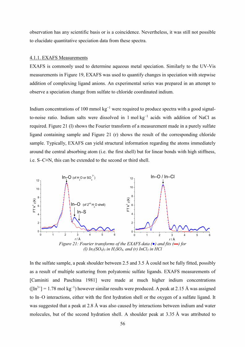
56

observation has any scientific basis or is a coincidence. Nevertheless, it was still not possible

to elucidate quantitative speciation data from these spectra.

4.1.1. EXAFS Measurements EXAFS is commonly used to determine aqueous metal speciation. Similarly to the UV-Vis

measurements in Figure 19, EXAFS was used to quantify changes in speciation with stepwise

addition of complexing ligand anions. An experimental series was prepared in an attempt to

observe a speciation change from sulfate to chloride coordinated indium.

Indium concentrations of 100 mmol kg−1 were required to produce spectra with a good signal-

to-noise ratio. Indium salts were dissolved in 1 mol kg−1 acids with addition of NaCl as

required. Figure 21 (l) shows the Fourier transform of a measurement made in a purely sulfate

ligand containing sample and Figure 21 (r) shows the result of the corresponding chloride

sample. Typically, EXAFS can yield structural information regarding the atoms immediately

around the central absorbing atom (i.e. the first shell) but for linear bonds with high stiffness,

i.e. S–C≡N, this can be extended to the second or third shell.

0 1 2 3 4 5 60

2

4

6

8

10

12

In–SIn–O (of 2nd H

2O shell)

In–O (of H2O or SO

4

2–)

FT k

2 (k

)

r / Å 0 1 2 3 4 5 6

0

2

4

6

8

10

12

FT k

2 (k

)

r / Å

In–O / In–Cl

Figure 21: Fourier transforms of the EXAFS data (●) and fits (▬) for

(l) In2(SO4)3 in H2SO4, and (r) InCl3 in HCl

In the sulfate sample, a peak shoulder between 2.5 and 3.5 Å could not be fully fitted, possibly

as a result of multiple scattering from polyatomic sulfate ligands. EXAFS measurements of

[Caminiti and Paschina 1981] were made at much higher indium concentrations

([In3+] = 1.78 mol kg−1) however similar results were produced. A peak at 2.15 Å was assigned

to In–O interactions, either with the first hydration shell or the oxygen of a sulfate ligand. It

was suggested that a peak at 2.8 Å was also caused by interactions between indium and water

molecules, but of the second hydration shell. A shoulder peak at 3.35 Å was attributed to

57

interactions between In3+ and the sulfur atom of an associated sulfate ligand. Caminiti et al.

also observed a small peak at 4.15 Å which they attributed to interactions between In3+ and

water molecules from the second hydration shell, however this was not seen in Figure 21 (l). It

would be possible to detect such interactions but only when sufficient measurements are made

such that a satisfactory background subtraction can be performed.

EXAFS measurements confirmed the presence of a 6.1(5) oxygen-coordinated indium

complex, with an average bond length of 2.169(9) Å. While these measurements could not

distinguish between the In–O interactions of associated water molecules and sulfate ligands,

results were consistent with the literature regarding aqueous [In(SO4)(H2O)5]+ complexes

[Caminiti and Paschina 1981] as well as bond lengths in the crystal structures of

InH(SO4)2·5H2O and InOH(SO4)(H2O)2 [Johansson, Seip et al. 1961].

In a purely chloride containing sample, the data and fit are in good agreement with each other,

and results are consistent with work from [Charnock, Henderson et al. 1999; Narita, Tanaka et

al. 2014; Seward, Henderson et al. 2000]. The average speciation in solution is an indium atom

surrounded by 2.9 ± 0.7 oxygen atoms and 3.5 ± 0.9 chlorine atoms, most likely a mixture of

the hydrated chloride complexes [InCl3(H2O)3] and [InCl4(H2O)2]–. This analysis is in

agreement with geochemical modelling predictions discussed later in section 6.2. The results

of the measurement series with increasing chloride concentration is described in Table 5. The

In–O and In–Cl bond lengths are consistent with the literature, [Seward, Henderson et al. 2000]

found In–O and In–Cl bond lengths of 2.14(1) and 2.40(1) Å respectively. As expected, the

number of chloride atoms included in the indium complex, increases with increasing chloride

concentration.

EXAFS is an extremely powerful tool to elucidate speciation, but the experimental

requirements for measurements (a tuneable x-ray source and hence a synchrotron) make it a

complex, expensive, and highly specialised technique. The goal of this work was to establish a

technique to quickly and easily establish indium speciation and stability, hence EXAFS is not

a practical technique for this work.

58

Table 5: EXAFS fit parameters of 100 mmol kg−1 In3+ in 1 mol kg−1 acids with the addition of NaCl

Sample Co-

ordinating atom

No. of atoms r / Å Speciation

Debye-Waller

factor / Å2

Fit index /

% In2(SO4)3 in

H2SO4

+ 100 mmol kg−1 NaCl

O Cl

6.5(4) 0.6(2)

2.149(6) 2.39(1)

[In(H2O)6]3+ and

[InCl(H2O)5]2+ 0.016(2) 0.002(3) 3.9 %

+ 500 mmol kg−1 NaCl

O Cl

3.3(1.0) 3.6(9)

2.09(3) 2.39(1)

[InCl3(H2O)3] and [InCl4(H2O)3]-

0.017(5) 0.012(3) 2.7 %

InCl3 in HCl O Cl

2.9(7) 3.5(9)

2.20(3) 2.44(1)

[InCl3(H2O)3] and [InCl4(H2O)3]–

0.009(6) 0.013(5) 7.0 %

4.2. Electrochemical Measurements

Potentiometric methods are an alternative approach to determine metal ion speciation and

stability. However these techniques require measurement of valid half wave reduction

potentials. Section 3.2.3 describes how half wave reduction potentials can be determined with

cyclic voltammetry, hence complementary CV measurements to the UV-Vis measurements

shown in Figure 19 were made.

-1.6 -1.4 -1.2 -1.0 -0.8 -0.6 -0.4 -0.2 0.0

-60

-40

-20

0

20

40

60

[In3+] = 100 mmol kg–1

[H+] = 1 mol kg–1

mol kg–1

[HSO4–] [Cl–]

In2(SO4)3 in H2SO4 1.15 In2O3 in H2SO4 1

InCl3 in H2SO4 1 0.3

In2(SO4)3 in HCl 0.15 1 InCl3 in HCl 1.3Cl–

mixedSO4

2–

j / m

A cm

-2

E / V

WE: GCERE: AgCl/Ag 3 mol kg–1 NaClCE: Pt

Figure 22: CVs of various 100 mmol kg−1 In3+ salts in 1 mol kg−1 acids.

Due to the acid concentration it is assumed that sulfuric acid is partially dissociated to HSO4–

None of the CVs in Figure 22 showed reversible electrode kinetics, and indium behaviour in

sulfate solutions showed a much more negative onset reduction potential and a significantly

smaller oxidation peak currents than in chloride solutions. Similarly to the UV-Vis

measurements, when solutions contained an excess of chloride ions i.e. In2(SO4)3 in HCl,

indium exhibited chloride-like behaviour (i.e. smaller deposition overpotential, larger

59

oxidation currents). However, in an excess of sulfate (InCl3 in H2SO4), sulfate-like behaviour

(i.e. large deposition overpotential, smaller oxidation currents) was not observed. The CV of

the mixed ligand sample showed a significantly less negative reduction onset potential, and

multiple reduction peaks, consistent with the UV-Vis measurements of InCl3 in H2SO4, mixed

speciation is indicated. Under these experimental conditions no valid In3+/0 half wave reduction

potentials could be determined, hence further investigations with alternative electrode

materials were made.

4.2.1. Influence of Electrode Material

One of the advantages of voltammetry is the ease at which an electrochemical set up can be

modified, specifically regarding the working electrode, where different electrodes have

different properties and potential windows. The most commonly used electrode surfaces are

the platinum (Pt) and glassy carbon electrodes (GCE) due to their chemical inertness, and the

large potential window of the GCE. The standard redox potential of In3+/0 vs SHE is –0.338 V

(equation 2). Due to the potential window of Pt in acidic solutions, Pt electrodes can be

excluded from these investigations [Bard and Faulkner 1980]. However, a variety of other

electrode surfaces were considered including the hanging mercury drop electrode (HMDE),

copper (Cu), indium (In), and gold (Au).

10 mmol kg−1 indium perchlorate was dissolved in 10 mmol kg−1 perchloric acid for the

following experiments. LiClO4 was included as an inert supporting electrolyte to supress

migration and maintain a constant ionic strength. Perchlorate is a weakly coordinating ligand,

allowing the analysis of hydrated In3+ ions. The resulting CVs shown in Figure 23 are plotted

in current density (mA cm–2) to remove the influence of various sized electroactive areas.

On both copper and gold surfaces, indium exhibited irreversible reduction and little or no

oxidation of In0 was recorded. Most likely the reduced indium metal formed stable alloys with

the electrode surfaces, possibly even diffusing into the bulk electrode. In3+ reduction on the

GCE showed substantial reduction overpotentials. The onset potential for indium reduction

was –0.78 V, compared to –0.46 V on the HMDE, however both reduction and oxidation waves

could be resolved. There was minimal deposition overpotential observed on the indium

electrode, however as expected, the oxidative stripping waves of the deposited metal and bulk

electrode did overlap. Additionally the indium electrode was easily passivated and preparing

the metal electrode surface for measurements was experimentally challenging.

60

-1.4 -1.2 -1.0 -0.8 -0.6 -0.4 -0.2 0.0

HMDE

GCE

Au

Cu

j / m

A c

m-2

E / V

5 m

A c

m-2

In

Figure 23: CVs of In3+/0 redox chemistry measured on various electrode surfaces

From these measurements it appears the HMDE is most suitable for the electrochemical

analysis of indium due to the apparent reversible redox behaviour of the In3+/0 couple. The GCE

could also be usable as long as the large reduction overpotential does not result in simultaneous

reduction of indium and water i.e. breakdown of the solvent at the end of the potential window.

Further analysis of indium electrochemistry with the GCE and HMDE are required.

4.2.2. Investigations with the Glassy Carbon Electrode

Advanced characterisation of indium electrochemistry on the CGE was carried out in non-

complexing perchlorate solutions as well as chloride and sulfate ligand containing samples.

-1.5 -1.0 -0.5 0.0

i / m

A

E / V

0.5

mA + 100 mmol kg–1 ClO4

–

+ 100 mmol kg–1 Cl–

+ 100 mmol kg–1 SO42–

-1.0 -0.9 -0.8 -0.7 -0.6 -0.5 -0.4

-75

-50

-25

0

25

i /

A

E / V

Eonset = –0.799 V –0.839 V

In3+ + 3 e– In0.

E = –0.533 V.

vs AgCl/Ag

Figure 24: (l) CVs on the GCE showing the changing electrochemical behaviour of indium in the

presence of various ligand anions (r) effects of ligands on reduction behaviour

61

In all samples nucleation loops were observed, a common result of inhibited metal deposition

on a GCE surface. With an AgCl/Ag (3 mol kg−1 NaCl) reference electrode, In3+ reduction is

expected around –0.53 V but it does not occur in these measurements until –0.8 V. The areas

of the oxidation peaks from indium stripping are significantly larger in samples containing

ligand anions. This corresponds to a larger amount of indium being deposited from these

solutions, therefore suggesting that chloride and sulfate complexes exhibit faster deposition

kinetics compared to aqua complexes. While it is possible to deposit indium onto a GCE from

all three solutions, deposition from chloride species occurs at a much smaller overpotential (see

Figure 24 (r) where the onset reduction potential in the sulfate sample is more negative than in

the chloride sample). While this is consistent with commonly made observations in the bulk

electroplating [Piercy and Hampson 1975] it is contrary to the stability of chloride complexes,

as the stabilisation of indium should shift the deposition potential to more negative values

compared to sulfate or aqua complexes. It is hence, a valid assumption that chloride has an

activating effect on the deposition kinetics of indium. The changes in electrochemical

behaviour in Figure 24 are indicative of changing speciation, which supports the UV-Vis

measurements in Figure 20 (l).

The shift in reduction potential of indium with changing chloride and sulfate concentration can

be clearly seen in Figure 25 where relatively small amounts of chloride can have a significant

effect on the electrochemical behaviour, and therefore speciation and stability, of indium.

-1.5 -1.0 -0.5 0.0

+ 500 mmol kg–1 Cl–

+ 50 mmol kg–1 Cl–

InCl3 in HCl

+ 5 mmol kg–1 Cl–

In3+:Cl– 1:13

In3+:SO42–:Cl– 1:11.5:5

In3+:SO42–:Cl– 1:11.5:0.5

In3+:SO42– 1:11.5

j / m

A c

m-2

E / V

50 m

A c

m-2

In3+:SO42–:Cl– 1:11.5:0.05

In2(SO4)3 in H2SO4

Figure 25: In3+ electrochemical behaviour with various concentrations of sulfate and chloride ligands

62

Despite the large potential window and hydrogen overpotential of the GCE, solvent breakdown

can still interfere with metal reduction. Two indications that this is occurring can be seen in

Figure 25: firstly the merging of the reduction waves of the analyte and solvent, and secondly

small steps in the reduction waves at negative potentials which indicate gas evolution at the

electrode surface.

To confirm the simultaneous reduction of indium and water, QCM measurements to determine

current efficiency were made. As described in section 3.2.4, EQCM methods can be used to

determine the ratio of deposited mass to total charge passed at the electrode surface, equivalent

to the number of electrons required to reduce or oxidise one atom of analyte. Traditional gold

QCM crystals coated with a thin glassy carbon layer were used for direct comparison with

earlier CV measurements.

0 50 100 150 200

-2

-1

0

1

2

3

4

5

6

i / m

A

t / s

0

2

4

6

m /

g

In3+ In0 C = 39.53 mCm = 5.894 g

7.98 e– / In

In0 In3+ C = 19.67 mCm = 6.881 g

3.40 e– / In

Figure 26: CV and QCM data (deposited mass) plotted against time

for current efficiency determination

In Figure 26 the ratio of charge to deposited mass yielded values of 7.98 and 3.40 electrons for

the reduction and oxidation of one indium atom respectively. Both values are higher than the

expected 3 electrons, but the significantly higher number of electrons required for the reduction

confirms the occurrence of side reactions, most likely the reduction of water at the electrode

surface (2 H2O + 2 e– ⇌ H2 + 2 OH–).

The combination of nucleation loops, i.e. effects of electrocrystallisation kinetics, and

simultaneous side reactions in these measurements was a clear indication that voltammetry on

63

a GCE would not be a suitable technique for the quantitative determination of speciation or

stability constants.

4.2.3. Investigations with the Hanging Mercury Drop Electrode

The CVs shown in Figure 24 measured on the GCE did not yield results from which valid half

wave reduction potentials could be determined. These measurements were repeated using a

hanging mercury drop electrode (HMDE) which forms amalgams with most metals, and no

nucleation loops or metal reduction overpotential were observed (see Figure 27).

When considering the CV of the perchlorate sample (depicted with a green line in Figure 27),

a good agreement between the oxidative and reductive charges were found, which were

0.276 mC and 0.291 mC respectively, indicating electrochemical reversibility. However CVs

of all indium solutions on the mercury electrode did not exhibit fully reversible behaviour.

Oxidation in a chloride environment showed a split peak indicating simultaneous oxidation of

multiple species and two separate redox couples could be observed in the sulfate sample.

-1.00 -0.75 -0.50 -0.25

+ 100 mmol kg–1 Cl–

+ 100 mmol kg–1 ClO4–

i /

A

E / V

+ 100 mmol kg–1 SO42–5

A

Figure 27: CVs of various indium samples measured on the HMDE

To more accurately investigate the reversibility of the In3+/0 couple on the HMDE, further

measurements were made using the non-complexing indium perchlorate solution. Firstly, CVs

were recorded at various scan speeds (see Figure 28) as a reversible couple would demonstrate

a linear relationship between scan rate, √𝑣, and peak current, ipc (see equation 47). The insert

in Figure 28 (l) shows the magnitude of the absolute cathodic peak currents, |ipc|, as well as the

R2 value which indicates the relationship with √𝑣 is non-linear.

64

Furthermore, the CV modelling software, DigiElch was used to model a CV measurement and

determine various thermodynamic and kinetic parameters. A comparison of the modelled

(blue) and experimentally determined (black) data and the resulting parameters are shown in

Figure 28 (r). The relationship between the peak potentials is not the value expected for a

reversible couple (Epc – Epa = 57.0/n mV (see section 3.2.3)), additionally the transfer

coefficient, α, determined by the model is less than the ideal value of 0.5.

-1.0 -0.8 -0.6 -0.4 -0.2

-1

0

1

2

3

4

5

6

7

2.0 2.5 3.0 3.5 4.0 4.5 5.0 5.5

0.6

0.8

1.0

1.2

1.4

R2 = 0.9819

|i pc| /

µA

v1/2 / (Vs-1)1/2

i /

A

E / V

scan rate / mV s-1

5 10 15 20 25 30

-1.0 -0.8 -0.6 -0.4 -0.2

-1

0

1

2

3

4

5

6

i /

A

E / V

E0 = 0.536(1) V = 0.33(7) ks = 0.0042(3) cm s–1

|Epc – Epa| = 75.1 mV 75.2 mV1

57/n = 19.0 mV

Figure 28: Investigations regarding the reversibility of the In3+/0 couple on the HMDE

(l) CVs at various scan speeds and (r) comparison with DigiElch modelling

The results of the investigations regarding the relationship between |ipc| and √𝑣, as well as the

values determined for the transfer coefficient and rate constant (ks is in the order of magnitude

10–3 cm s–1), all indicate quasi-reversible reduction of indium on the mercury electrode. Hence

mercury would be a suitable electrode material to determine indium half wave reduction

potentials if a method can be developed that produces valid results in ligand containing

solutions. Figure 27 shows that this is not the case for cyclic voltammetry, hence further

investigations of voltammetric methods on the HMDE (i.e. polarography) were required.

4.3. Summary of Qualitative Spectroscopic and Electrochemical Analyses

Electrochemical and spectroscopic measurements can yield qualitative and quantitative

information regarding indium in various ligand containing solutions. However, none of the

techniques discussed in this section could simply and effectively determine indium speciation.

Differences between the UV-Vis spectra of indium in the presence of various complexing

ligands implied that indium speciation changes could be observed. From the literature it is

known that multiple indium sulfate and chloride complexes are stable in aqueous solutions, i.e.

65

InSO4+ and In(SO4)2

– or InCl2+ and InCl4

–. Spectra could be categorised as showing chloride,

or sulfate-like activity, but it was not possible to elucidate the structures of these complexes.

During the analysis of indium sulfate EXAFS measurements, it was challenging to differentiate

between the interaction of indium with oxygen atoms from either the first hydration shell or

from a sulfate ligand. All results were consistent with previously reported literature but while

EXAFS is a reliable technique to confirm speciation, the challenging experimental

requirements means it is not possible to perform quick and simple speciation analyses.

Cyclic voltammetry measurements were made to complement the UV-Vis investigations.

Changes in speciation, and the resulting impact on electrochemical behaviour could be

observed but on the glassy carbon electrode simultaneous solvent breakdown or electrode

crystallisation kinetics made redox potentials impossible to determine.

Further investigations showed that indium reduction on the hanging mercury drop electrode

was a quasi-reversible electrode process. However in the presence of complexing ligands,

cyclic voltammetry did not consistently produce results that were suitable for the determination

of half wave reduction potentials. Hence further research into polarographic (specifically

differential pulse voltammetry) methods were developed, with the goal to quantitatively

determine speciation and stability constants.

66

5. Determining Indium Stability Constants

In this section the development of a differential pulse voltammetry procedure to simultaneously

determine both the speciation and stability constants of indium nitrate, sulfate, chloride, and

hydroxide complexes is presented. For detailed experimental methods see Appendix i.ii.iii.

Previous measurements showed mercury was a suitable electrode material for electrochemical

investigations of indium, however cyclic voltammetry was not a suitable technique to

determine half wave reduction potentials. Various polarographic procedures were investigated,

including variations with hanging and dropping mercury electrodes, as well as pulsed methods

(the theoretical fundamentals of these measurements are explained in sections 3.3 and 3.4).

-0.64 -0.60 -0.56 -0.52 -0.48 -0.44 -0.40

-0.7

-0.6

-0.5

-0.4

-0.3

-0.2

-0.1

0.0

0.1

measured

HMDE E1/2 / V DPV –0.538 LSV –0.536

SMDE DPV –0.518 Polarography –0.537

In3+/0 E = –0.533 V (vs AgCl/Ag)

i or

i /

A

E / V Figure 29: Reduction of 1 mmol kg−1 In3+recorded with polarography and DPV

with the hanging and dropping mercury electrode

From Figure 29 it is clear that measurements of In3+ reduction recorded on a static mercury

dropping electrode (SMDE) were significantly noisier than corresponding hanging drop

(HMDE) results. Furthermore differential currents recorded during pulsed measurements on

the SMDE were higher the expected zero current after In3+ reduction (observed on the HMDE),

a result that cannot be currently explained. During SMDE methods, a fresh electrode surface

is available at each measurement point, however the mechanical removal of the drop from the

capillary tip disturbed the sample solution giving rise to jumps in the recorded current. In

HMDE measurements, having a single drop for the entire measurement resulted in smooth

reduction peaks and waves for DPV and polarography respectively, where resulting determined

67

E1/2 values were in good agreement. All E1/2 values determined in these measurements are in

good agreement (± 2 mV) with the exception of the pulsed measurements on the SMDE which

deviated significantly from the expected value.

One advantage that DPV has over polarography cannot be observed in Figure 29, but instead

the analysis methods to yield half wave reduction potentials must be considered. To accurately

determine E1/2 from a polarogram, a secondary plot of E against log (ilim–i/i) must be produced

(equation 62), whereas determining E1/2 values from a DPV measurement only requires a

simple peak analysis and consideration of the pulse potential (equation 63).

Differential pulse voltammetry on the hanging mercury drop electrode produced fast, accurate,

and reproducible measurements from which half wave reduction potentials could be easily

calculated. It was hence decided, future potentiometric investigations to determine the

speciation and stability of indium would be carried out using DPV methods on the HMDE.

Measurement of E1/2 as a function of ligand concentration can yield both the speciation and

stability constant of a metal complex (see section 3.4). A series of DPV measurements are

made at increasing complexing ligand ion concentrations. The difference between E1/2 for the

reduction of the hydrated In3+ ion, and the E1/2 values for the reduction of complexed indium,

which become increasingly negative as ligand ion concentration is increased, is called ∆E1/2.

A plot of ∆E1/2 against the logarithmic ligand concentration yields data points through which a

series of linear fits can be made. The speciation of a complex, i.e. the x value for the complex

MLx, can be obtained from the gradient of these fits, and the stability constant, log βx, can be

determined from the y-axis intercept. It is essential to maintain both metal ion concentration

and ionic strength during one series of measurements. A DPV ‘titration’ technique was

developed which allowed precise changes in ligand ion concentration to be made to the sample

without effecting overall metal ion concentration, pH, or ionic strength.

5.1. Differential Pulse Voltammetry Titration Technique

To accurately control ligand concentration while maintaining a constant ionic strength,

measurements were made by adding a calculated amount of complexing ligand containing

‘titrant’ to a supporting electrolyte-containing ‘sample’. By having the same concentrations of

indium and acid in both solutions, and equivalent amounts of ligand and electrolyte ions; the

68

pH, indium concentration, and ionic strength of the sample was maintained, while the volume

and ligand concentration increased. Exact ligand concentration in the sample was calculated

from the concentration of the titrant and the new volume of the sample. DPVs were measured

at each titration step and E1/2 values were determined from the peak potentials. Furthermore

the reversibility of the reduction was investigated by determining W1/2 values, the peak width

at half height. Under the conditions of the DPV measurements (pulse potential, ΔE = 25 mV

and n = 3), the W1/2 of a fully reversible reduction would equal 36.5 mV, and a fully irreversible

reduction 73 mV [Oldham and Parry 1970].

The basis of the DPV titration samples was 1 mmol kg−1 In(ClO4)3 in 10 mmol kg−1 HClO4,

samples were acidic enough to supress indium hydrolysis and the indium concentration was

sufficient to yield DPV peaks that were reproducible and easy to analyse. Supporting

electrolyte concentration in the sample depended on the solubility of the alkali metal salt used

in the titrant, i.e. a DPV titration with a titrant containing Na2SO4 would require a sample with

a lower ionic strength than with Li2SO4 because the solubility of the sodium salt is lower.

5.1.1. Maintaining Ionic Strength

To maintain constant ionic strength throughout the DPV measurements a non-complexing

supporting electrolyte was added to the samples. KNO3 and LiClO4 are most commonly used

in such experiments and therefore measurements were recorded in both environments.

However results were inconsistent and calculated constants varied between electrolytes. For

example, two DPV titration series to investigate indium complexation with sulfate were

performed, both samples had an ionic strength of 1 mol kg−1, but one contained KNO3 and the

other LiClO4 as the supporting electrolyte. The stability constant for the InSO4+ species

determined in later sections in a nitrate electrolyte was log β1 = 1.77 ± 0.03, however in a

perchlorate electrolyte the value was log β1 = 2.85 ± 0.03. Due to the difference in these values,

it was considered that the electrolytes were not inert and were actually interacting with In3+

ions in the sample. Previous UV-Vis (section 4.1) and EXAFS measurements [Seward,

Henderson et al. 2000] did not indicate complexation of indium with perchlorate ions, but

[Tuck 1983] reported a stability constant for the InNO32+ complex of log β1 = 0.18 ± 0.08. Very

little literature is available on the stability of indium nitrate complexes, a fraction in comparison

to the chloride and sulfate systems. Furthermore, the accuracy of this data is questionable – the

value reported in the review from Tuck was labelled as ‘doubtful’.

69

In an attempt to detect InNO32+ and determine the nitrate concentration at which this species

forms, a DPV titration with a nitrate containing titrant was performed. Selected DPVs showing

the reduction of indium with varying nitrate concentration can be seen in Figure 30.

-0.60 -0.55 -0.50 -0.45 -0.40 -0.35 -0.30-0.25

-0.20

-0.15

-0.10

-0.05

0.00

[In3+] = 1 mmol kg–1

[H+] = 10 mmol kg–1

I = 3 mol kg–1 (LiClO4)

T = 293.45 K

i /

A

E / V

[NO3–] / mmol kg–1 40 100 200 300 600 800 1000

-3.0 -2.5 -2.0 -1.5 -1.0 -0.5 0.0 0.5

-18

-15

-12

-9

-6

-3

0

x = 0.29 ± 0.03 In3+ / InNO3

2+

x = 1.02 ± 0.12 InNO3

2+

log 1 = 0.40 ± 0.03

x = 0.0556 ± 0.0004 In3+

E

1/2 /

mV

log [NO3–] / mol kg–1

Figure 30: Selected DPVs (l) and plots (r) showing changing half wave reduction potentials for In3+/0 (▲) with nitrate ligand concentration, where linear fits (▬) are used to calculate x and βx

At nitrate concentrations below 100 mmol kg−1 there is no significant change in E1/2 values

with nitrate concentration and no measurable complexation of indium is occurring. Formation

of the InNO32+ complex is first observed at 100 mmol kg−1, indicated by an increase in the

calculated x value above this concentration. InNO32+ is only found in significant quantities in

nitrate concentrations above 1 mol kg−1 where the x value is equal to 1.0 ± 0.1. From these

measurements a stability constant of log β1 = 0.40 ± 0.03 for the InNO32+ complex was

determined.

These results show that in the presence of more than 1 mol kg−1 of nitrate ions, such as those

used to maintain ionic strength, InNO32+ complexes are formed. Hence, measurements of

indium stability constants made in a nitrate supporting electrolyte, would actually yield the

relative stability between the nitrate complex and the complex under investigation, rather than

from In3+. Previously published data determined under these conditions [Deichman, Rodicheva

et al. 1966; Mikhailova, Nacheva et al. 1969; Fridman, Sorochan et al. 1962], should therefore

be treated with caution if corrections for InNO32+ formation have not been made.

In DPV a change from a reversible to an irreversible process is accompanied by an increase in

peak width and a decrease in peak height. In Figure 30 (l) the DPV peaks can be seen at varying

nitrate concentrations and peak size and shape remain almost constant throughout (initially

peak height decreases with increasing nitrate concentration but after formation InNO32+ slowly

70

increasing peak height can be observed). This is in agreement with the peak width and half

height, W1/2, values where the difference between the first and last measurements (i.e. from

[NO3–] = 0 to 3 mol kg−1) is W1/2 = 60.18 mV and W1/2 = 61.13 mV respectively, indicating

quasi reversible In3+ reduction.

The alternative supporting electrolyte, LiClO4, was not expected to form indium complexes.

However the stability constant for the InSO4+ species determined in a perchlorate supporting

electrolyte (log β1 = 2.85 ± 0.03) was significantly larger than the IUPAC recommended

stability constant (log β1 = 1.78). Perchlorate ions can be reduced to yield chloride ions

(8 H+ + ClO4− + 8 e− → Cl− + 4 H2O) [Brown and Gu 2006] and previous CV measurements

(see Figure 25) have shown the significant impact that small concentrations of chloride ions

can have on the electrochemical behaviour of indium. During DPV titrations to determine

InSO4+ stability, it became clear, through spot tests with silver nitrate solution, that a slow

formation of small amounts of chloride ions from the breakdown of the supporting electrolyte

could not be prevented. Due to the higher affinity of indium for chloride over sulfate ions, this

had a significant effect on the resulting stability constant. The reason for this breakdown is

unknown, despite being observed by other groups [Kondziela and Biernat 1975]. The effects

are reproducible with various sources of chemicals but only occur when perchlorate and indium

are both present in acidic solutions, although the effect was most strongly observed in solutions

of perchloric acid. A possible explanation could be that perchlorate ions readily react with trace

impurities of organic molecules. However, because chloride evolution was quite significant

and only occurred in acidic samples when indium was present, it is rather suspected that there

may be catalytic effects of the indium ion to the breakdown of perchlorate. At this time these

findings cannot be fully explained. It is clear that stability constants for InSO4+ measured in

perchlorate media [Schischkova 1978; Ricciu, Secco et al. 2000; Tur'yan and Strizhov 1972]

should be treated with care.

The measurement series from Figure 30 describing the complexation of indium with nitrate

ions obviously required a LiClO4 support electrolyte as using KNO3 in the initial sample would

have been nonsensical. It was found that chloride evolution could be minimised in these

measurements by using a double jacketed AgCl/Ag 3 mol kg−1 KCl reference electrode, where

the outer electrolyte vessel contained 1 mol kg−1 KNO3 to minimise chloride-based electrolyte

leakage into the sample. Measurements must also be completed rapidly before chloride

evolution became too significant. Chloride evolution could not be totally supressed, and the

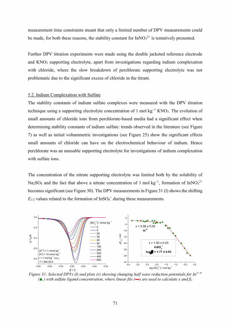
71

measurement time constraints meant that only a limited number of DPV measurements could

be made, for both these reasons, the stability constant for InNO32+ is tentatively presented.

Further DPV titration experiments were made using the double jacketed reference electrode

and KNO3 supporting electrolyte, apart from investigations regarding indium complexation

with chloride, where the slow breakdown of perchlorate supporting electrolyte was not

problematic due to the significant excess of chloride in the titrant.

5.2. Indium Complexation with Sulfate

The stability constants of indium sulfate complexes were measured with the DPV titration

technique using a supporting electrolyte concentration of 1 mol kg−1 KNO3. The evolution of

small amounts of chloride ions from perchlorate-based media had a significant effect when

determining stability constants of indium sulfate: trends observed in the literature (see Figure

7) as well as initial voltammetric investigations (see Figure 25) show the significant effects

small amounts of chloride can have on the electrochemical behaviour of indium. Hence

perchlorate was an unusable supporting electrolyte for investigations of indium complexation

with sulfate ions.

The concentration of the nitrate supporting electrolyte was limited both by the solubility of

Na2SO4 and the fact that above a nitrate concentration of 1 mol kg−1, formation of InNO32+

becomes significant (see Figure 30). The DPV measurements in Figure 31 (l) shows the shifting

E1/2 values related to the formation of InSO4+ during these measurements.

-0.65 -0.60 -0.55 -0.50 -0.45 -0.40 -0.35

-0.8

-0.6

-0.4

-0.2

0.0

i /

A

E / V

[SO42-] / mmol kg–1

0 5 20 30 40 50 100 200 300 400 600

[In3+] = 1 mmol kg–1

[H+] = 10 mmol kg–1

I = 1 mol kg–1 (KNO3)

T = 294.35 K

-3.5 -3.0 -2.5 -2.0 -1.5 -1.0 -0.5 0.0

-35

-30

-25

-20

-15

-10

-5

0

log [SO42–] / mol kg–1

x = 1.00 ± 0.03InSO4

+

log 1 = 1.77 ± 0.03

x = 0.06 ± 0.02In3+

E

1/2 /

mV

Figure 31: Selected DPVs (l) and plots (r) showing changing half wave reduction potentials for In3+/0

(▲) with sulfate ligand concentration, where linear fits (▬) are used to calculate x and βx

72

In Figure 31 (r), ΔE1/2 remains at essentially 0 mV up to a sulfate concentration of

approximately 30 mmol kg−1, indicating that up to this point, the speciation of the In3+ ion

remains unchanged. Above this concentration |ΔE1/2| increases and a linear fit through the data

points yields x = 1.00 ± 0.03, equating to the presence of a single sulfate ligand in the

coordination shell of indium. The stability constant calculated for InSO4+ in this measurement

is log β1 = 1.77 ± 0.03 which is in excellent agreement with work by [Deichman, Rodicheva et

al. 1966] who determined log β1 = 1.78 in 2 mol kg−1 NaNO3. However, the issues discussed

above imply that this value should be treated with reservations until it has been shown that

corrections for the formation of small amounts of InNO32+ are not required. An assessment of

the DPV curves in Figure 31 (l) show the reversibility of In3+ reduction is decreasing with

increasing sulfate concentration. In the absence of sulfate ligands W1/2 = 53.71 mV. As sulfate

concentration increases, so does W1/2 and when In3+ is reduced from a sulfate complex

W1/2 = 60.28 mV.

As one of the aims of this study was to determine the stability constants of indium under

conditions relevant to bioleaching, these titration measurements were repeated in ten-fold

excess concentrations (10 mmol kg−1) of iron and zinc, where the stability constants

determined for InSO4+ were log β1 = 1.79 ± 0.03 and log β1 = 1.88 ± 0.01 respectively. The

small impact that the presence of other metals have on stability constants determined with DPV,

means such values could be measured under conditions similar to that of leachate solutions.

When using a more soluble sulfate salt such as Li2SO4, the ionic strength of the supporting

electrolyte containing sample can also be increased. At a nitrate concentration of 3 mol kg−1,

the starting species of the differential pulse titration series is assumed to be InNO32+ rather than

In3+. As shown in Figure 32, this has a significant effect on the calculated stability constant for

the InSO4+ species, which in this measurement was determined to be log β1 = 1.27 ± 0.05

compared to log β1 = 1.77 ± 0.03 previously.

73

-0.6 -0.5 -0.4-0.25

-0.20

-0.15

-0.10

-0.05

0.00

[In3+] = 1 mmol kg–1

[H+] = 10 mmol kg–1

I = 3 mol kg–1 (KNO3)

T = 294.25 K

i /

A

E / V

[SO42-] / mmol kg–1

0 5 10 40 100 300 400 600 850 1000

-3.0 -2.5 -2.0 -1.5 -1.0 -0.5 0.0

-40

-30

-20

-10

0

x = 1.04 ± 0.07InSO4

+

log 1 = 1.27 ± 0.05

x = 2.05 ± 0.09In(SO4)2

–

log 2 = 1.64 ± 0.02

x = 0.14 ± 0.02InNO3

2+ / InSO4+

E

1/2 /

mV

log [SO42–] / mol kg–1

Figure 32: Selected DPVs (l) and plots (r) showing the changing half wave reduction potentials for In3+/0 (▲) with high sulfate ligand concentration, where linear fits (▬) are used to calculate x and βx

However, stability constants determined in these measurements become comparable when the

assumed intermediate complexes from the different reaction pathways of the two

measurements are considered. Direct formation of InSO4+ from In3+ has an associated stability

constant log β1 = 1.77 ± 0.03, but when InSO4+ is formed from an InNO3

2+ intermediate, two

stability constants must be considered:

In3+ + NO3

− → InNO32+

InNO32+ + SO4

2− → InSO4+ + NO3

−

log 𝛽1 = 0.40 ± 0.03

log 𝛽1 = 1.27 ± 0.05

(75)

(76)

In3+ + SO42− → InSO4

+ log 𝛽1 = 1.67 ± 0.08 (77)

The sum of the stability constants in equation 75 and 76 give the overall stability constant

log β1 = 1.67 ± 0.08 for the InSO4+ complex determined in a 3 mol kg−1 KNO3 supporting

electrolyte. The difference between the stability constants for the direct and indirect formation

of InSO4+ could be explained due to the difference in ionic strengths of the two measurements

but further analysis would be required to determine this experimentally. In section 6.1

geochemical modelling of indium speciation under the conditions of these DPV measurements

is presented. At nitrate concentration of 3 mol kg−1, the predicted concentration of InNO32+

surpasses that of In3+, which supports the assumption that the stability constant for the InSO4+

species from Figure 32 is likely the relative stability between InNO32+ and InSO4

+.

Due to the higher solubility of Li2SO4, and hence higher concentration of available sulfate

ligands, formation of the In(SO4)2– complex is also observed in this DPV titration. As with the

indirect formation of InSO4+, the formation constant relating to InNO3

2+ must be considered,

74

hence the calculated stability constant of the In(SO4)2– complex is log β2 = 2.04 ± 0.05. There

is less available literature regarding the stability of the higher order sulfate complexes (see

Figure 7), the value determined in this work sits within the range of previously determined

constants (1.8 ≤ log β2 ≤ 2.6), the value recommended by [Tuck 1983], log β2 = 2.53 ± 0.05, is

at the higher end of the data range. Indium reduction from the In(SO4)2– complex is almost

fully reversible with a W1/2 value of 45.05 mV.

5.3. Indium Complexation with Chloride

To determine the stability constants of indium complexes formed with chloride ions, a DPV

titration was performed with a NaCl containing titrant. Due to the higher solubility of NaCl

than Na2SO4, the following measurements had an ionic strength of 3 mol kg−1. LiClO4 was

used as a supporting electrolyte as the slow formation of small amounts of chloride ions from

the breakdown of the perchlorate supporting electrolyte was not problematic due to the large

excess of chloride containing titrant.

-0.70 -0.65 -0.60 -0.55 -0.50 -0.45 -0.40 -0.35

-3.5

-3.0

-2.5

-2.0

-1.5

-1.0

-0.5

0.0

[In3+] = 1 mmol kg–1

[H+] = 10 mmol kg–1

I = 3 mol kg–1 (LiClO4)

T = 293.25 K

i /

A

E / V

[Cl-] / mmol kg–1

0 3 7.5 10 15 20 30 40 80 200 600 1500 2989

-3.0 -2.5 -2.0 -1.5 -1.0 -0.5 0.0 0.5-120

-100

-80

-60

-40

-20

0

20

x = 4.1 ± 0.2InCl4

- log 4 = 4.49 ± 0.03

x = 2.0 ± 0.2InCl2

+ log 2 = 3.95 ± 0.09x = 1.45 ± 0.05

InCl2+ / InCl2+

x = 0.61 ± 0.07In3+/ InCl2+

E

1/2 /

mV

log [Cl–] / mol kg–1 Figure 33: Selected DPVs (l) and plots (r) showing changing half wave reduction potentials for In3+/0

(▲) with chloride ligand concentration, where linear fits (▬) are used to calculate x and βx

Complexation of indium with chloride ions described in Figure 33, is more complicated to

analyse than the sulfate measurement shown in Figure 31. E1/2 values are already changing at

chloride concentrations below 10 mmol kg−1, which is consistent with indium ions higher

affinity for chloride ions. However, until a chloride concentration of around 200 mmol kg−1 is

reached, gradients of the linear fits do not yield an integer value for x. This implies that at lower

chloride concentrations there is a mixed speciation of In3+, InCl2+ and InCl2+ complexes. The

fact that this is reflected in the DPV data shows that ligand exchange is sufficiently fast such

that this method can provide information on bulk speciation, and not only on single

electroactive species that may control electrodeposition kinetics. At chloride concentrations

75

between 200 to 400 mmol kg−1, the InCl2+ species alone dominates (x = 2.0 ± 0.2) and a

stability constant log β2 = 3.95 ± 0.09 is found. This is in good agreement with the

recommended value from [Tuck 1983] of log β2 = 3.71 ± 0.3. Above 500 mmol kg−1 chloride

concentration, the InCl4− species is present (x = 4.11 ± 0.23) with a stability of

log β4 = 4.49 ± 0.03 which is not dissimilar to work from [Hasegawa, Shimada et al. 1980] who

determined log β4 = 4.32.

Regarding reversibility, in the absence of chloride ligands, i.e. in 3 mol kg−1 LiClO4, a

W1/2 value of 62.5 mV was found. However, as indium is complexed by chloride ions,

reduction of indium from the InCl4– complex approaches reversibility and in 3 mol kg−1

chloride W1/2 = 41.35 mV. The fact that the reversibility of In3+ reduction differs between the

supporting electrolytes (in 3 mol kg−1 LiClO4, W1/2 = 62.5 mV and in 1 and 3 mol kg−1 KNO3,

W1/2 = 53.71 and 61.13 mV respectively), is another indication of the significant effects of

supporting electrolyte on these measurements, both with respect to ionic strength and also the

speciation of indium in the ‘non-complexing’ supporting electrolyte sample.

5.4. Indium Complexation with Hydroxide

The same DPV titration technique was adapted for the determination of indium hydrolysis

constants. The same principle was applied to maintain metal ion concentration and ionic

strength, but to observe formation of hydrolysis species, pH values would have to either

increase or decrease. Two complimentary techniques were developed: firstly starting from an

acidic indium solution and slowly increasing the pH with a hydroxide ion containing titrant

(here called a hydroxide titration), and secondly the reverse method, where the sample started

as a weakly acidic/neutral solution and pH was decreased by titrating with an acidic titrant

(here called a proton titration).

Both measurements required the sample pH to be continuously recorded. Unfortunately, the

design of the classic glass pH electrode allows small amounts of the internal KCl electrolyte to

enter the sample to protect the electrode from contamination from the sample (similar to the

AgCl/Ag reference electrode). As previously discussed, the resulting effect of chloride ions on

indium speciation obviously makes accurate analysis of In3+ hydrolysis impossible. To

overcome this issue, for one DPV titration series, two simultaneous titrations were made: both

samples underwent the same hydroxide or proton titration, but in one series DPV measurements

76

were made and in the other pH was recorded. As only trace amounts of KCl electrolyte was

leaking into the second sample, the impact of chloride concentration on pH should be

insignificant. This allowed the pH, and hence hydrolysis of indium, to be analysed during a

DPV titration series. In section 5.4.2 a mixed hydroxl-chloride complex is detected indicating

that higher chloride concentrations can significantly impact indium hydrolysis.

5.4.1. Hydroxide and Proton Titrations

As discussed in section 3.1.2, there are two ways to define a metal ion hydrolysis constant,

either by considering the addition of a hydroxide ligand (equation 32), or the deprotonation of

an associated water molecule (equation 33). In the former, the equilibrium considered in the

hydroxide titration, i.e. the definition of the stability constant, is comparable with the formation

of previous metal-ligand complexes, and hence the analysis method of the changing half wave

potentials is the same, i.e. plotting against the logarithmic OH– concentration as shown in

Figure 34 (top). Although it is important to note, in this case log K values rather than log β

values are determined. In the proton titration the defined stability constant is different, resulting

in a different equation for the changing half wave potential:

∆𝐸12

= − 2.303 𝑅𝑇

𝑛𝐹log 𝛽𝑥 −

2.303 𝑅𝑇𝑥

𝑛𝐹log [H+]−1 (78)

As shown in Figure 34 (bottom), in a proton titration ΔE1/2 must be plotted with respect to

log [H+]–1, or pH value, to yield the log β values of the indium hydrolysis species.

The results of both DPV titrations produced plots that looked unusual in comparison to

previous measurements. Firstly, the gradients of the ΔE1/2 plots were unexpected: during the

progression of a measurement series, higher order hydrolysis species are formed and hence the

number of complexing ligands, and therefore the x values of the subsequent linear regions,

should also be increasing in steepness. Furthermore, no integer values for x could be found.

Non-integer x values have been observed in previous measurements (mixed speciation at low

chloride concentrations), but in conjunction with the unusual shaped plots, mixed speciation

was not considered to be the lone cause. One possible explanation for this phenomenon could

be formation of polynuclear indium complexes.

77

-0.60 -0.55 -0.50 -0.45 -0.40 -0.35-3.0

-2.7

-2.4

-2.1

-1.8

-1.5

-1.2

-0.9

-0.6

-0.3

0.0

i /

A

E / V

Hydroxide Titration

[In3+] = 1 mmol kg–1

[H+]sample = 500 mmol kg–1

I = 500 mmol kg–1 (KNO3

-)

T = 293.85 K

pH value 0.364 0.406 0.447 0.715 1.070 1.358 1.403 1.432 1.502 1.508 1.527 1.546 1.567 1.588 1.612 1.637 1.664 1.692 1.718

-13.0 -12.5 -12.0 -11.5 -11.0 -10.5 -10.0

-10

-8

-6

-4

-2

0

2

4

6

E

1/2 /

mV

log [OH-] / mol kg–1

x = 0.69 ± 0.02

x = 0.37 ± 0.03

x = 0.06 ± 0.01

-0.60 -0.55 -0.50 -0.45 -0.40 -0.35-3.0

-2.5

-2.0

-1.5

-1.0

-0.5

0.0

3.612 3.300 3.083 2.974 2.745 2.711 2.575 2.481 2.318 2.221 2.196 2.060 1.951 1.863 1.810 1.607 1.431 1.241 0.654

[In3+] = 1 mmol kg–1

[H+]titrant = 500 mmol kg–1

I = 500 mmol kg–1 (KNO3)

T = 293.85 K

i /

A

E / V

Proton Titration

pH value

0.5 1.0 1.5 2.0 2.5 3.0 3.5

0

5

10

15

20

25

30

x = 0.11 ± 0.01x = 0.31 ± 0.01

x = 0.86 ± 0.03

E1/

2 / m

V

pH

x = 0.48 ± 0.05

Figure 34: Selected DPVs (l) and plots (r) showing changing half wave reduction potentials for In3+/0

in (top) hydroxide and (bottom) proton titrations. Arrows indicate measurement direction

So far in this work, the formation of polynuclear indium complexes has not been considered.

A potentiometric investigation by [Biederman 1956] suggested the formation a series of

polynuclear indium complexes: In2(OH)24+, In3(OH)4

5+ … Inn+1(OH)2n(n+3), however it was

unclear as to the number and significance of these species. The data presented by Biedermann

could also be explained by formation of a single polynuclear complex, In3(OH)45+, with a

stability constant log β = –9.27 ± 0.02.

While the presence of polynuclear complexes could not be proven conclusively in the scope of

this work, two techniques were used to provide support for this hypothesis. Firstly, hydroxide

titration measurements were repeated at lower indium concentrations in an attempt to minimise

formation of In3(OH)45+. In a hydroxide DPV titration at an indium concentration of

1 mmol kg−1 (see Figure 34 (top)), a ligand number ligand of x = 0.69 ± 0.02 was found between

hydroxide concentrations of log [OH–] = –13 and –12 (i.e. between pH 1 and 2). At a lower

indium concentration of 0.1 mmol kg−1, the corresponding x value was 0.93 ± 0.09 which could

be attributed to the formation of the InOH2+ complex. A stability constant log K1 = 10.8 ± 0.9

78

was found which using the equation log β = log K + x log Kw (see section 3.1.2), equates to

log β1 = –3.2 ± 0.9 which is in fairly good agreement with the literature value log β1 = –4.00

from [Baes and Mesmer 1976]. At low indium concentrations, DPV peaks are smaller and

hence the error in these measurements is increased and therefore not ideal for stability constant

determination.

The second method to provide evidence of polynuclear indium species was to reanalyse the

gradients of the ΔE1/2 plots presented in Figure 34 taking into account the possible presence of

In3(OH)45+, namely that the number of electrons involved in the reduction reaction is now n = 9

rather than 3. This could be an oversimplification of the reduction mechanism, as a (kinetically

slow) indirect breakdown of the polynuclear complex is likely. The re-analysis of the ΔE1/2

plots is presented in Figure 35.

-13.0 -12.5 -12.0 -11.5 -11.0 -10.5 -10.0 -9.5

-10

-8

-6

-4

-2

0

2

4

6

8

E 1/

2 / m

V

log [OH-] / mol kg–1

x = 2.07 ± 0.05In3(OH)4

5+ In(OH)2+

log K = 25.6 ± 0.7

x = 1.12 ± 0.08In(OH)2

+ In(OH)3

log K = 14.1 ± 0.9

x = 0.21 ± 0.04

0.5 1.0 1.5 2.0 2.5 3.0 3.5 4.0

0

5

10

15

20

25

30

x = 0.94 ± 0.04In3(OH)4

5+ In(OH)3

log = –2.9 ± 0.1

x = 2.57 ± 0.08In3(OH)4

5+ InOH2+ / In(OH)2+

log = –6.4 ± 0.1

x = 0.33 ± 0.03In3(OH)4

5+

E

1/2 /

mV

pH

x = 1.4 ± 0.1In3(OH)4

5+ In3+ / InOH2+

log = –5.2 ± 0.1

Figure 35: Re-analysis of changing half wave potential plots for (l) the hydroxide and (r) the proton

titration where presence of polynuclear indium complex In3(OH)45+ is considered

The re-analysed results for the hydroxide titration (Figure 35 (l)) initially looked encouraging,

specifically regarding the x values which are now closer to integer values, but the determined

log K values were unusually large. Similarly to the determination of the In(SO4)2– stability

constant, where the intermediate formation of InNO32+ must also be considered, the assumption

that polynuclear indium complexes are formed means any resulting hydrolysis constants must

consider the In3+ ⇌ In3(OH)45+ equilibrium. From the analysis of the hydroxide titration, the

following stability constants were determined using the literature stability constant for

In3(OH)45+, log β = –9.27 ± 0.02 [Biederman 1956]. Both log K and log β values are given

below, interchanged using the equation log β = log K + x log Kw described in section 3.1.2:

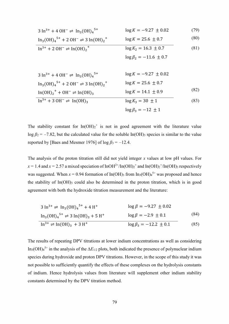
79

3 In3+ + 4 OH− ⇌ In3(OH)4

5+

In3(OH)45+ + 2 OH− ⇌ 3 In(OH)2

+

log 𝐾 = −9.27 ± 0.02

log 𝐾 = 25.6 ± 0.7

(79)

(80)

In3+ + 2 OH− ⇌ In(OH)2

+ log 𝐾2 = 16.3 ± 0.7

log 𝛽2 = −11.6 ± 0.7

(81)

3 In3+ + 4 OH− ⇌ In3(OH)45+

In3(OH)45+ + 2 OH− ⇌ 3 In(OH)2

+

In(OH)2+ + OH− ⇌ In(OH)3

log 𝐾 = −9.27 ± 0.02

log 𝐾 = 25.6 ± 0.7

log 𝐾 = 14.1 ± 0.9

(82)

In3+ + 3 OH− ⇌ In(OH)3 log 𝐾3 = 30 ± 1

log 𝛽3 = −12 ± 1

(83)

The stability constant for In(OH)2+ is not in good agreement with the literature value

log β2 = –7.82, but the calculated value for the soluble In(OH)3 species is similar to the value

reported by [Baes and Mesmer 1976] of log β3 = –12.4.

The analysis of the proton titration still did not yield integer x values at low pH values. For

x = 1.4 and x = 2.57 a mixed speciation of InOH2+/In(OH)2+ and In(OH)2

+/In(OH)3 respectively

was suggested. When x = 0.94 formation of In(OH)3 from In3(OH)45+ was proposed and hence

the stability of In(OH)3 could also be determined in the proton titration, which is in good

agreement with both the hydroxide titration measurement and the literature:

3 In3+ ⇌ In3(OH)4

5+ + 4 H+

In3(OH)45+ ⇌ 3 In(OH)3 + 5 H+

log 𝛽 = −9.27 ± 0.02

log 𝛽 = −2.9 ± 0.1

(84)

In3+ ⇌ In(OH)3 + 3 H+ log 𝛽3 = −12.2 ± 0.1 (85)

The results of repeating DPV titrations at lower indium concentrations as well as considering

In3(OH)45+ in the analysis of the ∆E1/2 plots, both indicated the presence of polynuclear indium

species during hydroxide and proton DPV titrations. However, in the scope of this study it was

not possible to sufficiently quantify the effects of these complexes on the hydrolysis constants

of indium. Hence hydrolysis values from literature will supplement other indium stability

constants determined by the DPV titration method.

80

5.4.2. Mixed Hydroxide Species

[Baes and Mesmer 1976] noted formation of indium hydrolysis complexes are hindered by the

presence of chloride. This is consistent with the high stability of indium chloride complexes.

Typically formation of hydrolysis products starts at pH 2, but at high chloride concentrations

this can be delayed until above pH 4. This stabilisation was attributed to a mixed hydroxy-

halide complex, InClOH+, formed from the mono-chloride complex with a stability constant of

log β1 = –0.63 [Ferri 1972b].

To detect the mixed hydroxy-halide species with DPV, a proton titration was performed where

both the sample and titrant had a chloride ion concentration of 15 mmol kg−1. Previous DPV

measurements (see Figure 33) had indicated that between 0 to 20 mmol kg−1 chloride, a mixed

In3+ and InCl2+ speciation was present. Unlike in other experiments, where the desired starting

indium speciation was In3+, in this measurement, due to the chloride concentration and weakly

acidic pH, the starting speciation would theoretically be InClOH+. As the proton titration

progressed, pH would decrease, and the hydroxy-chloride complex would be protonated to

InCl2+, the associated equilibrium constant would be the inverse of the formation of InClOH+

from InCl2+.

0.8 0.7 0.6 0.5 0.4 0.3 0.2

-1.35

-1.20

-1.05

-0.90

-0.75

-0.60

-0.45

-0.30

-0.15

0.00

2.950 2.862 2.754 2.698 2.521 2.423 2.347 2.239 2.106 1.890 1.556 1.380 1.012 0.822 0.602

[In3+] = 1 mmol kg–1

[Cl-] = 15 mmol kg–1

[H+]titrant = 485 mmol kg–1

I = 500 mmol kg–1 (LiClO4)

T = 300.55 K

i /

A

E / V

pH value

0.4 0.6 0.8 1.0 1.2 1.4 1.6 1.8

-10

-8

-6

-4

-2

0

2

4

6

x = –0.18 ± 0.01InClOH+

x = –0.81 ± 0.03InClOH+ InCl2+

log 1 = 0.77 ± 0.03

E

1/2 /

mV

pH Figure 36: Selected DPVs (l) and plots (r) showing changing half wave reduction potential for In3+/0

plotted against pH, for a proton titration in 15 mmol kg−1 Cl–

In Figure 36 initially small changes in ΔE1/2 indicated little or no changes in speciation from

InClOH+, however as pH decreased a negative trend in ΔE1/2 could be seen. This resulted in an

x value of –0.89 ± 0.03 which was attributed to the loss of a single hydroxide ligand. The

stability constant calculated for the protonation of InClOH+ was log β1 = 0.77 ± 0.03 (see

equation 86), hence the stability constant associated with the formation of InClOH+ from InCl2+

81

is log β1 = –0.77 ± 0.03 (see equation 87). This value is in good agreement with the literature,

log β1 = –0.63 [Ferri 1972b].

InClOH+ ⇌ InOH+ + Cl−

InOH+ + Cl− ⇌ InClOH+

log 𝛽1 = 0.77 ± 0.03

log 𝛽1 = −0.77 ± 0.03

(86)

(87)

5.5. Summary of Quantitative Determination of Indium Speciation and Stability

A differential pulse voltammetry technique has been applied to quickly and simply determine

the stability constants of indium with various complexing ligands. By measuring the effect of

increasing ligand concentration on the half wave reduction potential of indium, speciation and

stability could be determined simultaneously. Measurements were fast and simple: depending

on the number of titration steps, the combined measurement and analysis time was usually less

than 6 hours. Initially complexation with nitrate, chloride, and sulfate ligands was successfully

investigated. The methodology was adapted to determine hydrolysis constants however it was

not possible to quantify the effect polynuclear indium complexes had on the resulting

calculated values. The significantly larger errors that accompanied the experimentally

determined hydrolysis constants meant that values from the literature determined by other

methods were preferable for geochemical modelling. The higher stability of the indium

hydroxy-halide complex inhibited polynuclear complex formation and hence it was possible to

determine the stability of the InClOH+ species.

A summary of all the experimentally determined stability constants from this section is given

in Table 6. Suitable stability constants will now be included in geochemical modelling software

to produce speciation models. Initially these models will be compared to simple solutions but

later they will be applied to process relevant solutions to determine the chemical behaviour of

target metals as required.

82

Table 6: Stability constants determined with DPV and their suitability for geochemical modelling, compared to literature values [Tuck 1983; Baes and Mesmer 1976; Hasegawa, Shimada et al. 1980]

Equilibrium Constant log βx

Complex Experimental Literature Geochemical Modelling?

InNO32+ 0.40 ± 0.03 0.18 ± 0.08

InSO4+ 1.77 ± 0.03 1.78 ± 0.02

In(SO4)2 – 2.04 ± 0.05 2.53 ± 0.05

InCl2+ 3.95 ± 0.09 3.71 ± 0.3

InCl4– 4.49 ± 0.03 4.32

InClOH+ –0.77 ± 0.03 –0.63

InOH2+ –3.2 ± 0.9 –4.00

In(OH)2+ –11.6 ± 0.7 –7.82

In(OH)3 –12.2 ± 0.1 –12.4

83

6. Geochemical Modelling

In this section geochemical modelling (see section 3.6) will first be used to model simple

indium containing samples. Speciation will be predicted in samples with various indium

concentrations, ligand ion concentrations, and pH values, and compared to experimentally

determined results. The models designed in this section can then be later adapted to predict

behaviour in more complex systems. For the PHREEQC input files see Appendix ii.

6.1. Modelling of Indium Complexation with Nitrate, Sulfate, and Chloride

Input files were written so that PHREEQC, in conjunction with the BHMZ database, produced

speciation diagrams. Initially the speciation of indium in increasing nitrate, sulfate, and

chloride concentrations was modelled (for the PHREEQC input files see Appendix ii.i).

In the model, the sodium salts of nitrate, sulfate, and chloride were added stepwise to 1 kg of

water containing 1 mmol kg−1 In3+ at 25 °C. PHREEQC adjusted pH (pH 1 ± 0.05) and redox

potential (E = 237 ± 45 mV) to maintain charge balance and redox equilibrium respectively.

The resulting models had a residual error of 0.08 % after 14 iterations. One method to test the

validity of the model produced with experimentally determined constants, is to compare the

results when the BHMZ database includes stability constants from the literature and

experimentally determined stability constants. This comparison is shown in Figure 37.

As discussed in section 3.6.2, stability constants selected for the BHMZ database were

critically evaluated, regarding both the accuracy of their determination and the conditions under

which they were determined (high ionic strength). In general, constants determined

experimentally in this work did not differ significantly from the selected literature values,

hence resulting modelled speciation is also similar. The similarities between these results

indicate the critical assessment of literature values for the BHMZ database (i.e. selecting

accurate values determined at high ionic strength) was successful. The only major differences

in predicted speciation can be seen at high sulfate concentrations where the ratio between

InSO4+ and In(SO4)2

– is shifted, as well as the relationship between InCl2+ and InCl2+ at

intermediate chloride concentrations.

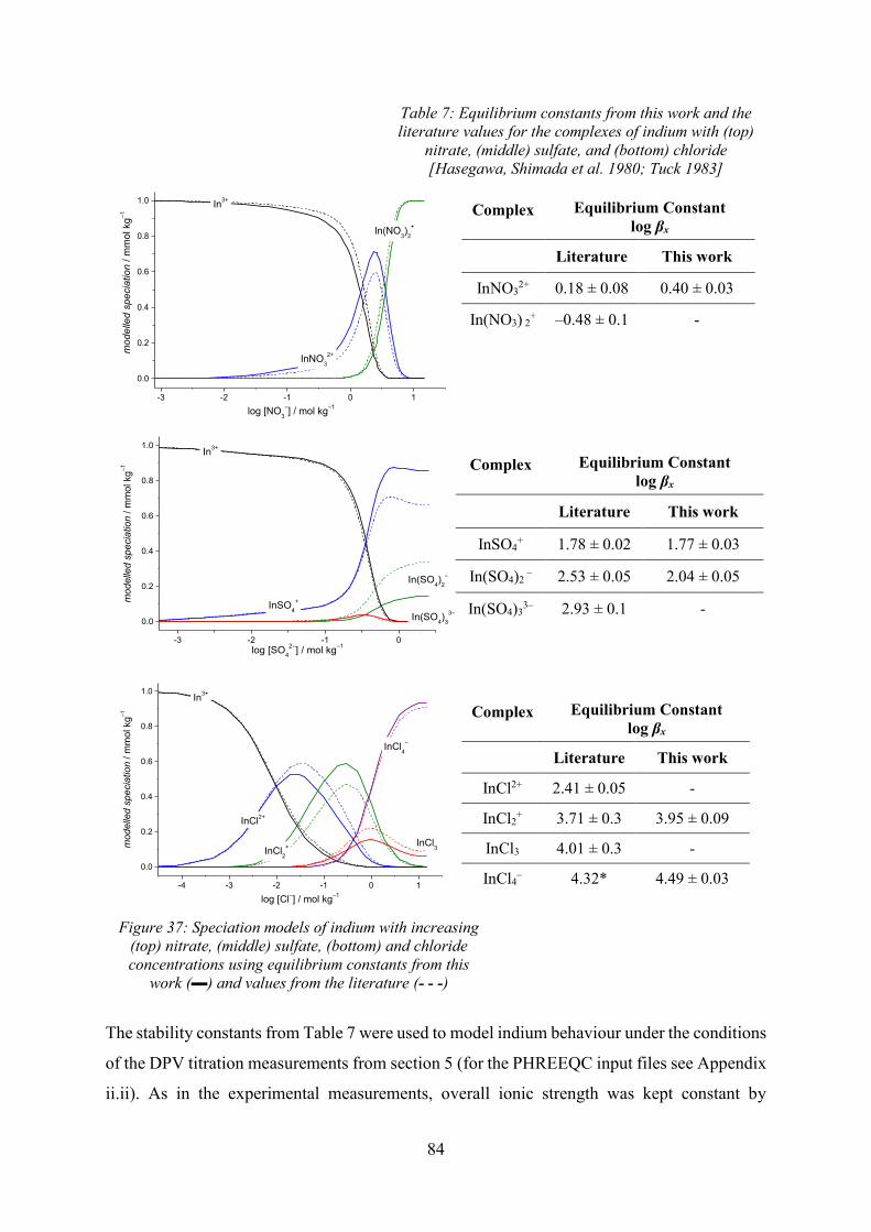
84

Table 7: Equilibrium constants from this work and the literature values for the complexes of indium with (top)

nitrate, (middle) sulfate, and (bottom) chloride [Hasegawa, Shimada et al. 1980; Tuck 1983]

-3 -2 -1 0 1

0.0

0.2

0.4

0.6

0.8

1.0

In(NO3)2+

InNO32+m

odel

led

spec

iatio

n / m

mol

kg–1

log [NO3–] / mol kg–1

In3+

Complex

Equilibrium Constant log βx

Literature This work

InNO32+ 0.18 ± 0.08 0.40 ± 0.03

In(NO3) 2+ –0.48 ± 0.1 -

-3 -2 -1 0

0.0

0.2

0.4

0.6

0.8

1.0

In(SO4)33–

mod

elle

d sp

ecia

tion

/ mm

ol k

g–1

log [SO42–] / mol kg–1

In3+

InSO4+

In(SO4)2–

Complex

Equilibrium Constant log βx

Literature This work

InSO4+ 1.78 ± 0.02 1.77 ± 0.03

In(SO4)2 – 2.53 ± 0.05 2.04 ± 0.05

In(SO4)33– 2.93 ± 0.1 -

-4 -3 -2 -1 0 1

0.0

0.2

0.4

0.6

0.8

1.0

InCl4–

InCl3InCl2+

InCl2+

In3+

mod

elle

d sp

ecia

tion

/ mm

ol k

g–1

log [Cl–] / mol kg–1

Complex

Equilibrium Constant log βx

Literature This work

InCl2+ 2.41 ± 0.05 -

InCl2+ 3.71 ± 0.3 3.95 ± 0.09

InCl3 4.01 ± 0.3 -

InCl4– 4.32* 4.49 ± 0.03

Figure 37: Speciation models of indium with increasing (top) nitrate, (middle) sulfate, (bottom) and chloride concentrations using equilibrium constants from this

work (▬) and values from the literature (- - -)

The stability constants from Table 7 were used to model indium behaviour under the conditions

of the DPV titration measurements from section 5 (for the PHREEQC input files see Appendix

ii.ii). As in the experimental measurements, overall ionic strength was kept constant by

85

increasing the complexing ligand concentration at the same rate as supporting electrolyte

concentration was decreased. The plots of changing half wave potentials from section 5 are

compared to the speciation models in Figure 38 to Figure 40.

-3.0 -2.5 -2.0 -1.5 -1.0 -0.5 0.0 0.5

-18

-15

-12

-9

-6

-3

0 x = 0.29 ± 0.03 In3+ / InNO3

2+

x = 1.03 ± 0.12 InNO3

2+

log 1 = 0.41 ± 0.03

x = 0.0556 ± 0.0004 In3+

E

1/2 /

mV

log [NO3–] / mol kg–1

0.0

0.2

0.4

0.6

0.8

1.0

m

odel

led

spec

iatio

n / m

mol

kg–1

InNO32+

In3+

In(NO3)2+

Figure 38: Changing half wave reduction potentials (▲) compared to modelled speciation (▬)

plotted against nitrate concentration

The initial speciation of free In3+ in the model is consistent with unchanging ΔE1/2 values,

which indicate no measurable complexation of indium. As nitrate concentration increases,

formation of InNO32+ is observed in the model and analysis of the DPV data over the same

concentration range shows a mixed In3+ and InNO32+ speciation. As nitrate concentration

approaches 1 mol kg−1, concentrations of the InNO32+ species surpasses In3+ in the model, and

this is also reflected in ΔE1/2 values. While formation of In(NO3)2+ can be seen in the model,

nitrate concentrations in the DPV measurements are not sufficiently high enough for this

species to form at predominant concentrations.

The model clearly demonstrates the presence of indium nitrate complexes at concentrations

consistent with those used to maintain ionic strength. This can also be seen in the models

describing the DPV titration experiments with sulfate, where KNO3 at various concentrations

was used as a supporting electrolyte.

86

-3.5 -3.0 -2.5 -2.0 -1.5 -1.0 -0.5 0.0-35

-30

-25

-20

-15

-10

-5

0

InNO32+

InSO4+

In3+

x = 1.00 ± 0.03 InSO4

+

log 1 = 1.77 ± 0.03

x = 0.06 ± 0.02In3+ / InNO3

+E

1/2 /

mV

log [SO42–] / mol kg–1

0.0

0.2

0.4

0.6

0.8

1.0

In(SO4)2–

mod

elle

d sp

ecia

tion

/ mm

ol k

g–1

-3.0 -2.5 -2.0 -1.5 -1.0 -0.5 0.0 0.5

-50

-40

-30

-20

-10

0

InNO32+

x = 1.04 ± 0.07InSO4

+

log 1 = 1.27 ± 0.05

In(SO4)2–

InSO4+

x = 2.05 ± 0.09In(SO4)2

-

log 2 = 1.64 ± 0.02

x = 0.15 ± 0.02InNO3

2+ / In3+

E

1/2

/ mV

log [SO42–] / mol kg–1

In3+

0.0

0.2

0.4

0.6

0.8

mod

elle

d sp

ecia

tion

/ mm

ol k

g–1

Figure 39: Changing half wave reduction potentials (▲) compared to modelled speciation (▬)

plotted against sulfate concentration where the supporting electrolyte was (l) 1 mol kg−1 KNO3 and (r) 3 mol kg−1 KNO3

As a DPV measurement progresses, supporting electrolyte concentration is steadily decreased

as complexing ligand is increased to maintain overall ionic strength. When using a 1 mol kg−1

KNO3 supporting electrolyte, initial nitrate and sulfate concentrations would be 1 and

0 mol kg−1 respectively but this would be almost reversed by the end of the measurement

(nitrate concentration decreases but never reaches 0 mol kg−1). Ideally under these conditions,

initial indium speciation would be free In3+, however the model in Figure 39 (l) shows the

InNO32+ species is also present. Above a sulfate concentration of 10 mmol kg−1, the

significantly more stable InSO4+ complex begins to form in the model, and this is reflected in

the changing E1/2 values shortly after. The presence of a small amount of the nitrate complex

does not appear to have a significant impact on the stability constant for InSO4+ determined in

this measurement. It is in good agreement with values determined in other supporting

electrolytes, hence no corrections regarding the initial presence of InNO32+ were made in these

measurements.

However, when DPV measurements were made with lithium rather than sodium sulfate salts,

the corresponding KNO3 supporting electrolyte concentration must also be increased. When

these higher concentrations are included in the model, initially concentrations of the indium

nitrate complex dominated over free indium (Figure 39 (r)). In the DPV titration this

corresponded to an effect on the experimentally determined stability constant for InSO4+

(log β1 = 1.27 ± 0.05 compared to log β1 = 1.77 ± 0.03 previously), however corrections could

be made for the formation of the nitrate complex, and then the stability constants for InSO4+

determined in the DPV titrations of both concentrations of sulfate were in fairly good

agreement. In the model shown in Figure 39 (r), formation of the In(SO4)2– complex begins

87

slowly above a sulfate concentration of 200 mmol kg−1 and this was reflected in the high sulfate

concentration DPV measurements above 400 mmol kg−1. The higher stability of In(SO4)2–

means formation is observed in the changing E1/2 values despite concentrations of InSO4+ being

in considerable excess.

In Figure 40, the ΔE1/2 values imply that at very low chloride concentrations there is mixed

speciation of In3+ and InCl2+ which is consistent with the prediction of the geochemical model.

InCl2+ formation begins as chloride concentration is increased, but it is not until 200 mmol kg−1

that InCl2+ is the dominant species in the model, consistent with the DPV analysis. Above a

chloride concentration of 500 mol kg−1, the more stable InCl4– complex is reflected in the

changing E1/2 values, this coincides with the chloride concentration at which predicted

formation of InCl4– becomes significant.

-3.0 -2.5 -2.0 -1.5 -1.0 -0.5 0.0 0.5

-140

-120

-100

-80

-60

-40

-20

0

20

x = 4.11 ± 0.23InCl4

– log 4 = 4.49 ± 0.03

InCl4–

InCl3

InCl2+

InCl2+

x = 2.02 ± 0.20InCl2

+ log 2 = 3.95 ± 0.11

x = 1.45 ± 0.05InCl2+ / InCl2

+

x = 0.61 ± 0.07In3+/ InCl2+

E

1/2 /

mV

log [Cl–] / mol kg–1

In3+

0.0

0.2

0.4

0.6

0.8

1.0

mod

elle

d sp

ecia

tion

/ mol

kg–1

Figure 40: Changing half wave reduction potentials (▲) compared to modelled speciation (▬)

plotted against chloride concentration

6.2. Modelling of Indium Hydrolysis

As selective precipitation is a useful tool in metal extraction and processing, a geochemical

model was used to predict the formation of soluble and insoluble indium hydroxide species. It

was not possible to accurately determine all indium hydrolysis constants experimentally.

However, unlike in the formation of indium sulfate and chloride complexes, where stability

constants differ between multiple sources, the hydrolysis constants of indium listed in Table 8

from a review by [Baes and Mesmer 1976] are widely accepted.

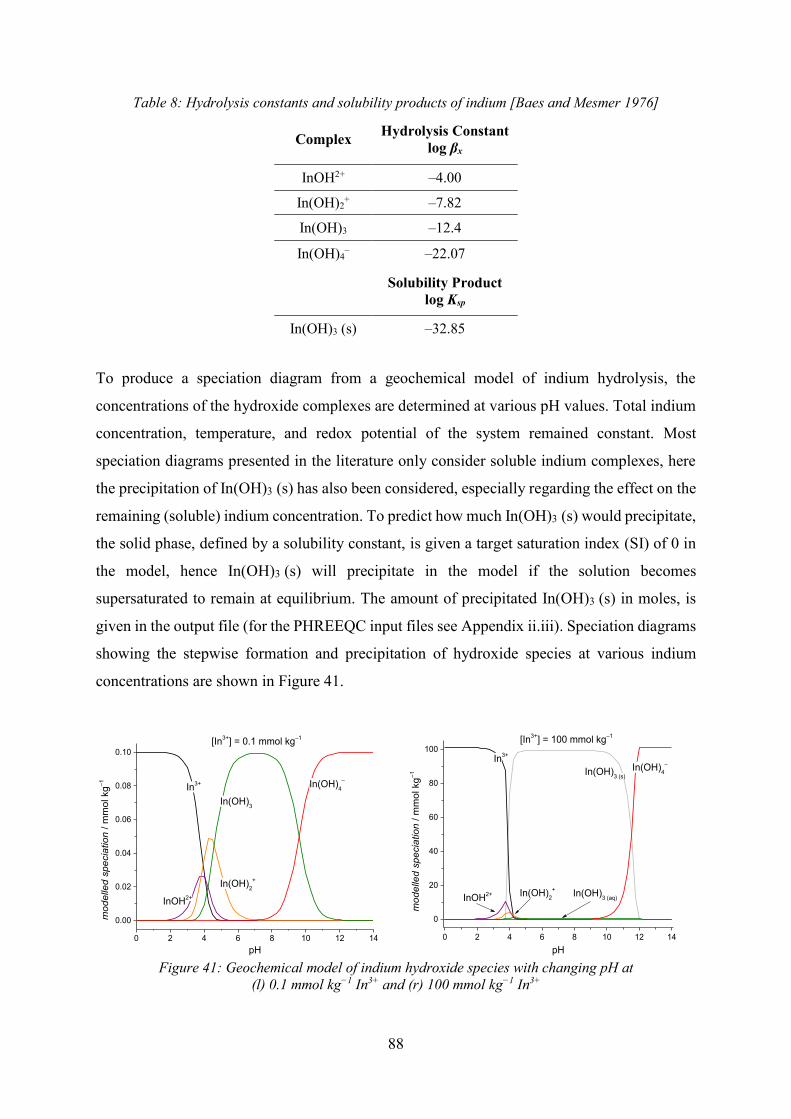
88

Table 8: Hydrolysis constants and solubility products of indium [Baes and Mesmer 1976]

Complex Hydrolysis Constant log βx

InOH2+ –4.00 In(OH)2

+ –7.82 In(OH)3 –12.4 In(OH)4

– –22.07

Solubility Product log Ksp

In(OH)3 (s) –32.85

To produce a speciation diagram from a geochemical model of indium hydrolysis, the

concentrations of the hydroxide complexes are determined at various pH values. Total indium

concentration, temperature, and redox potential of the system remained constant. Most

speciation diagrams presented in the literature only consider soluble indium complexes, here

the precipitation of In(OH)3 (s) has also been considered, especially regarding the effect on the

remaining (soluble) indium concentration. To predict how much In(OH)3 (s) would precipitate,

the solid phase, defined by a solubility constant, is given a target saturation index (SI) of 0 in

the model, hence In(OH)3 (s) will precipitate in the model if the solution becomes

supersaturated to remain at equilibrium. The amount of precipitated In(OH)3 (s) in moles, is

given in the output file (for the PHREEQC input files see Appendix ii.iii). Speciation diagrams

showing the stepwise formation and precipitation of hydroxide species at various indium

concentrations are shown in Figure 41.

0 2 4 6 8 10 12 14

0.00

0.02

0.04

0.06

0.08

0.10

InOH2+

In(OH)2+

[In3+] = 0.1 mmol kg–1

mod

elle

d sp

ecia

tion

/ mm

ol k

g–1

pH

In3+

In(OH)3

In(OH)4–

0 2 4 6 8 10 12 14

0

20

40

60

80

100

In(OH)3 (s)

mod

elle

d sp

ecia

tion

/ mm

ol k

g–1

pH

In3+

In(OH)4–

InOH2+ In(OH)2+ In(OH)3 (aq)

[In3+] = 100 mmol kg–1

Figure 41: Geochemical model of indium hydroxide species with changing pH at

(l) 0.1 mmol kg−1 In3+ and (r) 100 mmol kg−1 In3+

89

Figure 41 (l) shows that at a concentration of 0.1 mmol kg−1, all indium species are soluble. In

comparison, precipitation of insoluble In(OH)3 (s) can been seen over a wide pH range at higher

indium concentrations in Figure 41 (r). The amphoteric nature of indium means that soluble

species are formed at either very high or low pH values.

6.2.1 Modelling of Polynuclear and Mixed Hydroxy-Halide Indium Complexes

During the experimental determination of hydrolysis constants (see section 5.4), results

indicated the presence of polynuclear indium complexes. Effects of polynuclear species were

not seen in DPV titrations of other ligand anions, where pH remained constant around pH 1.7,

hence formation of In3(OH)45+ was not expected to be seen in the model until above pH 2.

When the stability constant for the polynuclear indium species In3(OH)45+ was included in the

BHMZ database, it can be seen from Figure 42, formation of the polynuclear indium species

dominates at moderate pH values in concentrated indium solutions. The effect was only noticed

when using DPV titration methods to determine hydrolysis constants because of the pH range

of these measurements.

0 2 4 6 8 10 12 14

0

20

40

60

80

100

In3(OH)45+

mod

elle

d sp

ecia

tion

/ mm

ol k

g–1

pH

In3+

InOH2+

In(OH)2+

In(OH)3 (s) In(OH)4–

In(OH)3 (aq)

[In3+] = 100 mmol kg–1

Figure 42: Distribution of the hydrolysis products of indium,

including polynuclear In3(OH)45+ and precipitation of In(OH)3 (s)

Inclusion of the polynuclear species in the model has an impact on indium solubility, in Figure

41 precipitation of In(OH)3 (s) can be seen from pH 3.75, but In3(OH)45+ supresses formation

of In(OH)3 (s) and in Figure 42 precipitation is not predicted until pH 4.25.

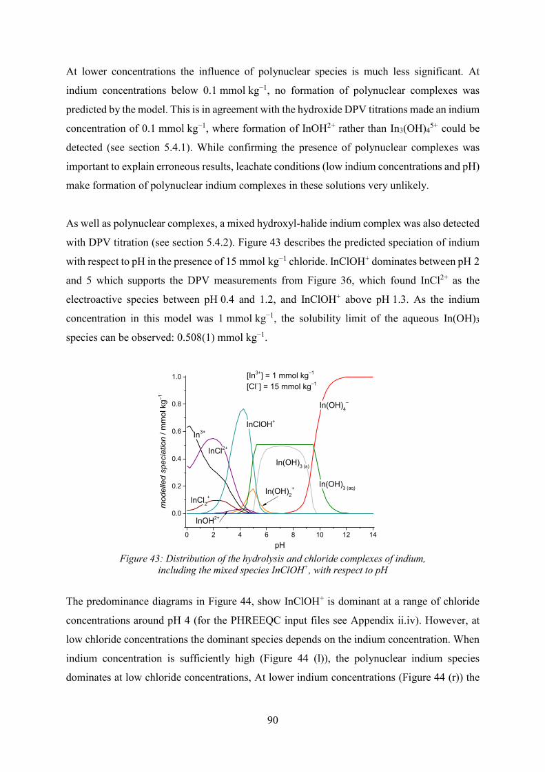
90

At lower concentrations the influence of polynuclear species is much less significant. At

indium concentrations below 0.1 mmol kg−1, no formation of polynuclear complexes was

predicted by the model. This is in agreement with the hydroxide DPV titrations made an indium

concentration of 0.1 mmol kg−1, where formation of InOH2+ rather than In3(OH)45+ could be

detected (see section 5.4.1). While confirming the presence of polynuclear complexes was

important to explain erroneous results, leachate conditions (low indium concentrations and pH)

make formation of polynuclear indium complexes in these solutions very unlikely.

As well as polynuclear complexes, a mixed hydroxyl-halide indium complex was also detected

with DPV titration (see section 5.4.2). Figure 43 describes the predicted speciation of indium

with respect to pH in the presence of 15 mmol kg−1 chloride. InClOH+ dominates between pH 2

and 5 which supports the DPV measurements from Figure 36, which found InCl2+ as the

electroactive species between pH 0.4 and 1.2, and InClOH+ above pH 1.3. As the indium

concentration in this model was 1 mmol kg−1, the solubility limit of the aqueous In(OH)3

species can be observed: 0.508(1) mmol kg−1.

0 2 4 6 8 10 12 14

0.0

0.2

0.4

0.6

0.8

1.0 [In3+] = 1 mmol kg–1

[Cl–] = 15 mmol kg–1

In(OH)2+

InOH2+

InCl2+

In(OH)3 (aq)

In(OH)3 (s)

In(OH)4–

InClOH+

InCl2+

In3+

mod

elle

d sp

ecia

tion

/ mm

ol k

g–1

pH Figure 43: Distribution of the hydrolysis and chloride complexes of indium,

including the mixed species InClOH+, with respect to pH

The predominance diagrams in Figure 44, show InClOH+ is dominant at a range of chloride

concentrations around pH 4 (for the PHREEQC input files see Appendix ii.iv). However, at

low chloride concentrations the dominant species depends on the indium concentration. When

indium concentration is sufficiently high (Figure 44 (l)), the polynuclear indium species

dominates at low chloride concentrations, At lower indium concentrations (Figure 44 (r)) the

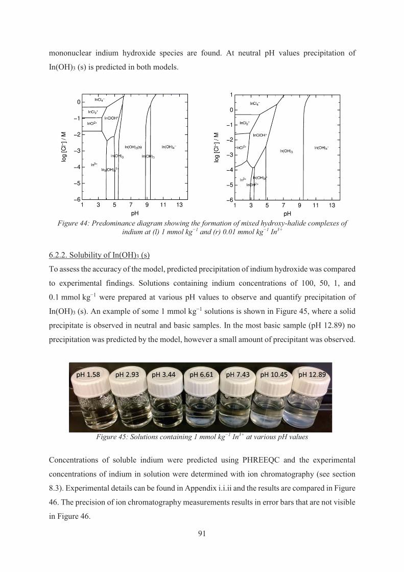
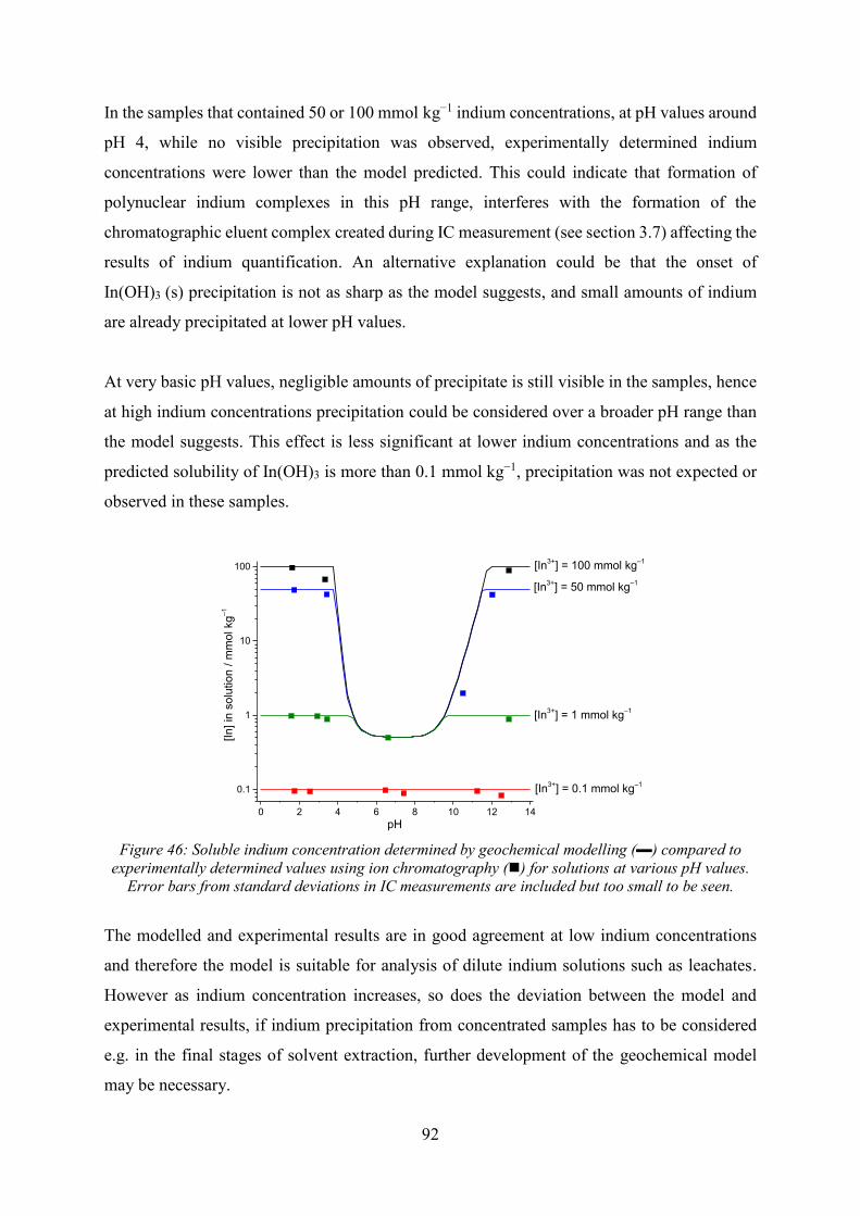
92

In the samples that contained 50 or 100 mmol kg−1 indium concentrations, at pH values around

pH 4, while no visible precipitation was observed, experimentally determined indium

concentrations were lower than the model predicted. This could indicate that formation of

polynuclear indium complexes in this pH range, interferes with the formation of the

chromatographic eluent complex created during IC measurement (see section 3.7) affecting the

results of indium quantification. An alternative explanation could be that the onset of

In(OH)3 (s) precipitation is not as sharp as the model suggests, and small amounts of indium

are already precipitated at lower pH values.

At very basic pH values, negligible amounts of precipitate is still visible in the samples, hence

at high indium concentrations precipitation could be considered over a broader pH range than

the model suggests. This effect is less significant at lower indium concentrations and as the

predicted solubility of In(OH)3 is more than 0.1 mmol kg−1, precipitation was not expected or

observed in these samples.

0 2 4 6 8 10 12 14

0.1

1

10

100

[In3+] = 50 mmol kg–1

[In3+] = 100 mmol kg–1

[In3+] = 0.1 mmol kg–1

[In3+] = 1 mmol kg–1

[In] i

n so

lutio

n / m

mol

kg–1

pH

Figure 46: Soluble indium concentration determined by geochemical modelling (▬) compared to experimentally determined values using ion chromatography () for solutions at various pH values.

Error bars from standard deviations in IC measurements are included but too small to be seen.

The modelled and experimental results are in good agreement at low indium concentrations

and therefore the model is suitable for analysis of dilute indium solutions such as leachates.

However as indium concentration increases, so does the deviation between the model and

experimental results, if indium precipitation from concentrated samples has to be considered

e.g. in the final stages of solvent extraction, further development of the geochemical model

may be necessary.

93

6.3. Summary of Geochemical Modelling of Model Indium Solutions

A database of experimentally determined stability constants has been produced, which, in

conjunction with self-written PHREEQC input files, allowed the successful modelling of

simple indium systems. Predicted speciation of indium with increasing ligand ion

concentrations was consistent with results from DPV titrations, and modelled behaviour of

hydroxide species was in good agreement with precipitation experiments of indium at low

concentrations. In chapter three, these models will be adapted and applied to project relevant

solutions, however to accurately model speciation in such samples, concentrations of the key

components must first be determined.

94

7. Chromatographic Methods

From the polysulfide leaching mechanism of metal sulfides, it is known that key leachate

components will be various metal ions and sulfur species. The following section will discuss

high pressure liquid chromatography (HPLC) and ion chromatography (IC) techniques which

were adapted to quantify sulfur species, in particular polysulfides, and metal ion concentrations

in process relevant solutions respectively. Chromatographic methods were selected for this

work because they offered a fast and accurate method for separating and quantifying both

aspects of the leachate. As described in section 3.7, polysulfide complexes were separated by

their polarity using a C18 column and a methanol-ammonium acetate eluent, and metal ions by

the stability of complexes formed with the eluent pyridine-2,6-dicarboxylic acid (PDCA) on

the CS5A column. For detailed experimental methods see Appendix i.iv.

7.1. Determining Sulfur Species with High Pressure Liquid Chromatography

The chemistry of sulfur compounds is important in many geochemical and biogeochemical

processes [Sand, Schippers et al. 1995; Schippers, Sand et al. 1996; Schippers, Rohwerder et

al. 1999], especially when considering their significant effect on redox processes. However,

due to the transitory nature of these unstable compounds, quantification has always been

challenging i.e. difficulties in sample preservation.

There are a wide range of aqueous sulfur species, including but not limited to sulfur (S0),

sulfide (S2–), sulfite (SO32–), thiosulfate (S2O3

2–), sulfate (SO42–), polysulfides (Sx

2–), and

polythionates (SxO62–). To assign and/or quantify these species, UV-Vis [Szekeres 1974; Koh

1990; Wincott and Vaughan 2006], IR and Raman [Milićev and Stergaršek 1989; Bondarenko

and Gorbaty 1997; Pokrovski and Dubrovinsky 2011; Wincott and Vaughan 2006; Holman,

Thompson et al. 2002], and electrochemical methods such as polarography and voltammetry

have been used [Luther, Giblin et al. 1985; Henneke, Luther et al. 1997; Ciglenečki and

Ćosović 1997; Rozan, Theberge et al. 2000; Umiker, Morra et al. 2002]. Sulfur species such

as SO42– and SO3

2– are easy to quantify with conventional anionic-IC methods [O’Reilly,

Dicinoski et al. 2001; Moses 1984; Kaasalainen and Stefánsson 2011; Hansen, Richter et al.

2002].

Due to the intermediates formed during the leaching of sphalerite, in this work determination

of sulfur species was focussed on polysulfides. Inorganic polysulfide chains have the general

95

formula Sx2-, or in their protonated form: H2Sx. Despite low concentrations, polysulfides may

play a significant role in environmentally relevant processes, i.e. metal precipitation [Chadwell,

Rickard et al. 1999; Luther 1991], due to their redox reactivity and high nucleophilicity.

There is little available literature regarding polysulfide analysis. Absorption studies

[Giggenbach 1972] and subsequent modelling [Teder 1971] has been carried out, as well as pH

titration [Schwarzenbach and Fischer 1960] techniques. One analytical method proposed

stabilisation with methylating agents, followed by gas chromatography and mass spectrometry

(GC-MS) [Korchevin, Turchaninova et al. 1991]. However, polysulfides chains of four or more

sulfur atoms are temperature sensitive and were destroyed in GC-MS analysis. Methylation

was effective at stabilising polysulfide chains but HPLC was preferable for analysis

[Kamyshny, Goifman et al. 2004; Kamyshny, Ekeltchik et al. 2006; Rizkov, Lev et al. 2004;

Steudel, Holdt et al. 1989; Dominko, Demir-Cakan et al. 2011; Kawase, Shirai et al. 2014].

Analysis of polysulfides can be separated into three areas: i) determining total concentration,

ii) separation, and iii) elucidating speciation [Kamyshny, Ekeltchik et al. 2006]. While total

polysulfide concentration can be readily determined, effective separation and quantification,

especially of ‘real-life’ samples, remains challenging. Until recently, there was a consensus

that individual spectra of different polysulfides could not be obtained, even the exact number

of polysulfide species existing in aqueous media is disputed today. Some authors believe that

the pentasulfide (S52–) is the longest polysulfide in water [Schwarzenbach and Fischer 1960;

Teder 1971; Giggenbach 1972] while others state that hexasulfide (S62–) is also likely to be

present in aqueous systems [Boulegue and Michard 1978].

7.1.1. Analysis of Polysulfides

The technique developed here was built on a combination of the work of [Kawase, Shirai et al.

2014] and [Kamyshny, Goifman et al. 2004], who both used HPLC to separate and assign

polysulfides. The significant difference between this work and the previously published

techniques was the inert environment in which those studies took place, attempting to minimise

polysulfide oxidation. As the overall aim of this study was to develop a methodology which

allowed quick and simple analysis of polysulfides in leachate solutions, where it would not

always be practical to work in an oxygen-free environment, i.e. sampling in underground

mines, in this work all derivatisation and separation of polysulfides took place under ambient

atmospheric conditions.

96

Kawase successfully used benzyl chloride as a polysulfide stabilising agent but due to

immiscibility with water, all polysulfide solutions were prepared in methanol. Kamyshny

prepared aqueous polysulfide solutions and simultaneously added methyl triflate and methanol

to bring capped polysulfides into the organic phase. Additionally, they characterised

disproportionation rates in the methanol/water mixture and determined the rate of polysulfide

methylation was sufficiently fast (0.375 seconds after methylation, more than 95 % of

polysulfides had reacted with MeOTf).

As all hydrometallurgical processes would be occurring in aqueous solutions, a successful

derivatisation technique was essential in aqueous samples. The technique of Fehér [Brauer

1954] was adapted to prepare a sodium polysulfide standard which was then diluted in

methanol to prepare a sample with a total polysulfide concentration of 10 mmol kg−1 (see

Appendix i.i.ii). Benzyl chloride was added to the polysulfide-methanol sample, after 30

seconds the yellow sodium polysulfides had been converted to colourless benzyl-polysulfides

(Bz2Sx).

The sample was carried through a reverse phase C18 column in a methanol-ammonium acetate

eluent mixture and after column separation the polysulfides passed through a UV-Vis detector

(see Appendix i.iv.i). The relevant section of the resulting chromatogram can be seen in Figure

47 (l). A large peak at ~1.5 minutes relating to the excess benzyl chloride did not interfere with

the polysulfides and is not included. The size of this peak can be slightly reduced by decreasing

the volume of benzyl chloride used during derivatisation, but this dramatically increases the

length of the derivatisation process. The benefits to a fast derivation process, i.e. preserving

polysulfide chain lengths, outweigh the relatively unproblematic benzyl chloride signal.

Kamyshny reported that the retention times of the various polysulfides have a logarithmic

dependence on chain length, which allowed identification of polysulfide species without the

use of reference materials. The relationship presented in Figure 47 (r) is linear for longer chain

polysulfides but non-linear for short chains Bz2S to Bz2S3.

There are considerable variations between the concentrations of polysulfides in the standard

solution. Significantly smaller peaks, and thus concentrations, of the more unstable longer

chains are found in comparison to the shorter chains. However, despite the ambient nature of

97

sample preparation conditions, it was still possible to detect long chain polysulfides up to a

chain length of 8 sulfur atoms.

2 3 4 5 6 7 8 9 10 11 12 13 14 150

400

800

1200

1600

2000

2400

Bz 2S

- 2.

221

Bz 2S

8 - 1

2.34

5

Bz 2S

7 - 9

.038

Bz 2S

6 - 6

.813

Bz 2S

5 - 5

.122

Bz 2S

4 - 3

.855B

z 2S3 -

3.1

57

coun

ts /

mA

U

t / min

Bz 2S

2 - 2

.522

8 9 10 11 12 13

0

5

10

t / min

1 2 3 4 5 6 7 80.2

0.3

0.4

0.5

0.6

0.7

0.8

0.9

1.0

1.1

log

(Rt)

/ min

Bz2Sx

relationship between retention time (Rt) and chain length (x)

Figure 47: (l) HPLC chromatogram showing retention times of benzyl-polysulfides separated by chain length, (r) relationship between logarithmic retention time and chain length

The polysulfide standard solution was diluted in methanol to produce samples containing total

polysulfide concentrations between 10 and 0.01 mmol kg−1 to determine the detection limits of

these species (for experimental details see Appendix i.i.ii). As shown in Figure 48, detection

of more stable mid-length chains was possible at low concentration but detection limits of more

unstable long and short chain polysulfides were much higher. Samples were measured

periodically over six month and showed no changes in peak areas or retention time, further

demonstrating the stability of the capped polysulfides.

Insert a) shows detection of shorter chain polysulfides Bz2S3 to Bz2S6 at total polysulfide

concentrations of 10 µmol kg−1 and insert b) shows the longer chain polysulfides Bz2S7 and

Bz2S8 can only be detected above 1 mmol kg−1. Additionally, the small peak related to the

shortest polysulfide chain, Bz2S2 and Bz2S, can only be seen above 100 µmol kg−1. In solutions

above 5 mmol kg−1, the signal related to Bz2S6 is distorted by an overlapping peak. In an

attempt to identify the source of this signal, samples that contained only sulfate, sulfide, or

sulfur were also analysed with HPLC, as other sulfur species are likely candidates. The only

measurements that resulted in a detectable signal was solutions containing elemental sulfur.

The retention time of Bz2S6 and sulfur are very similar under these conditions, hence the

overlapping peak. These peaks can be separated by changing eluent flow rate, temperature, or

the ratio of methanol and ammonium acetate (i.e. eluent polarity).

98

4 6 8 10 12 14 16 18 20 22 24 26

0.5 mmol kg–1c

0.2 mmol kg–1c

0.1 mmol kg–1c

0.01 mmol kg–1

10 mmol kg–1

5 mmol kg–1

2 mmol kg–1

1 mmol kg–1

0.5 mmol kg–1B

z 2S

(b)

Bz2S6

20 m

AU

coun

ts /

mA

U

t / min

10 mmol kg–1

5 mmol kg–1

2 mmol kg–1

1 mmol kg–1

0.5 mmol kg–1

0.2 mmol kg–1

0.1 mmol kg–1

0.01 mmol kg–1

Bz 2S

2S

Bz2S7

Bz2S8

1000

mA

U

100

mA

U

Bz2S3

Bz2S4

Bz2S5

Bz2S6

Bz2S3

Bz2S4

Bz2S5(a)

16 18 20 22 24 26

6 8 10 12 14 16

Figure 48: Chromatograms of polysulfide standard solutions at concentrations, (a) the detection of short chain polysulfides at concentrations down to 10 µmol kg−1

(b) the detection of longer chain polysulfides only possible down to ~1 mmol kg−1

In the later stages of this work this promising derivatisation and detection technique will be

used to quantify polysulfides in leachate samples.

7.2. Determining Metal Ion Concentration with Ion Chromatography

As discussed in section 3.7.1, for the chromatographic analysis of metal ions, they must be

complexed in the mobile phase. Two common complexing eluents are oxalic acid and

pyridine-2,6-dicarboxlic acid (PDCA). The high thermodynamic stability of the iron oxalate

complex (Fe(Ox)33– log K = 18.5) [Weiß 2001] inhibits ion-exchange through Donnan

exclusion. Hence, determination of iron using an oxalic acid eluent is impossible. Lead cannot

be spectroscopically detected after separation on the CS5A column with PDCA, the stability

of Pb(PDCA)22– is higher than the that of the UV-active complex (Pb(PAR)2) formed during

post column derivatisation.

One of the aims of the BHMZ is to produce leaching solutions with an indium concentration

of 10 mg l−1 as this is a viable concentration for subsequent extraction processes. For initial

testing concentrations of all metal ions were 10 mg l−1, however in leaching samples the

concentrations of iron and zinc are expected to be in considerably higher than indium.

For a comprehensive list of all quantifiable metal ions, standard solutions were prepared for

metal ions that were expected to be found in the leachate, these were then measured in an oxalic

99

acid and PDCA eluent. Retention times of metal ions in Figure 49 vary between the eluents

due to the differing stability constants of the metal complexes formed with PDCA and oxalic

acid respectively.

2 4 6 8 10

0

200

400

600

800

1000

coun

ts /

mA

U

t / min

Pb2+

Cu2+

Cd2+

Co2+

Zn2+

Ni2+

Oxalic Acid Eluent

t / min Pb3+ 2.63Cu2+ 3.06Cd2+ 4.08Co2+ 5.66Zn2+ 7.51Ni2+ 9.10

4 6 8 10 12 14 16

0

100

200

300

400

500

600

700

Co2+

Fe2+

Ni2+

Zn2+

In3+

coun

ts /

mA

Ut / min

Cu2+

PDCA Eluent

Cd2+

Fe3+

Mn2+

t / min Fe3+ 5.58Cu2+ 7.26In3+ 7.43Ni2+ 8.22Zn2+ 9.08Co2+ 10.12Cd2+ 11.17Mn2+ 12.10Fe2+ 13.39

Figure 49: Chromatograms of 10 mg L−1 metal standards measured in (l) oxalic acid and (r) PDCA

Almost all metal ions expected to be found in the leachate could be detected, with the exception

of chromium and arsenic. While a PDCA eluent allowed detection of more metal ions, the

separation of nickel, zinc, and cadmium was better in oxalic acid making quantification easier.

Indium could not be measured in an oxalic acid eluent, and in the PDCA eluent indium had

almost the same retention time as copper, this would cause them to co-elute in a mixed sample.

Retention times are usually unique to various ions thus allowing simultaneous analysis of

complex solutions. However, when retention times are insufficiently separated overlapping of

peaks can occur, under these circumstances it is almost impossible to obtain a quantitative

analysis.

7.2.1. Raised Temperature Ion Chromatography

IC measurements with a column such as the Dionex Ion Pac CS5A are typically done at a

column temperature of 30 °C, however at this temperature on the CS5A column, indium and

copper are impossible to differentiate. Other groups have reported the separation of indium

from zinc [Kawazu and Kakiyama 1978], cadmium [Strelow 1988], and other trace elements

in manganese [Faisca and Victor 1988] using IC. Previous methods to isolate group 13 metals

from ferric iron, copper, lead, and zinc [Yan, Zhang et al. 1988] involved precise control of

pH, chloride concentration, and temperature as well as complex pre and post-column

treatments. To achieve the separation of indium from other common leachate components,

variation of the column temperature was investigated.

100

Initially the dependence of retention times on temperature was established using standard

solutions. At 20 °C indium had a retention time of 8.49 minutes which was shifted to

6.20 minutes at 45 °C. This was a significantly larger shift than for all other metals, including

copper which shifted from 7.62 to 6.86 minutes over the same temperature range. Thus, at both

the lower and higher limits of the investigated temperature range, copper and indium peaks

were separated. However, when multiple element standards were prepared, it became clear that

at 20 °C the retention time of indium directly overlaps with nickel.

By measuring chromatograms across a range of temperatures, it is possible to track the shifting

indium peak. At 45 °C five distinct quantifiable peaks can be resolved, chromatograms and

resulting metal ion retention times can be seen in Figure 50.

2 4 6 8 10 12

0

54

x

x

x

x

x

x

20 oC

25 oC

30 oC

35 oC

40 oC

coun

ts /

mA

U

t / min

45 oC500

mA

U

(45 °C) t / min1. Fe3+ 4.432. In3+ 6.203. Cu2+ 6.864. Ni2+ 7.705. Zn2+ 8.33

1 2 3

Figure 50: Chromatographs showing the relationship between retention time and temperature for a

sample containing 10 mg L−1 Fe3+, In3+, Cu2+, Ni2+, and Zn2+

This technique would allow quick and simple simultaneous determination of most of the metal

ion concentrations found in the leachate, assuming the more complex background matrix of the

leachates does not affect metal ion separation on the column.

7.2.2. Stability of Indium in the Chromatographic Eluent

To prepare a calibration series for the quantitative analysis of indium, indium solutions up to

40 mg L–1 were prepared from a 1 g L–1 in 0.5 mol kg−1 HNO3 IC-grade standard solution. At

higher indium concentrations, and thus higher nitric acid concentrations, resulting

chromatograms displayed indium peaks with shoulders. Thus, measurements of 10 mg L–1

101

indium standards in various nitric acid concentrations were made (Figure 51 (a)). Peak

shoulders, and eventually peak splitting, could be seen with increasing nitric acid

concentration. To isolate the cause to either increasing H+ or NO3– concentrations, the

measurements were repeated in increasing HCl and KNO3 concentrations (Figure 51 (b) and

(c)). Due to the buffer behaviour of the eluent, which is in considerable excess, it was unlikely

that changing sample pH would have a significant effect on the resulting chromatogram. This

was confirmed by varying nitrate concentration while pH remained constant, where peak

splitting was also induced.

0

75

150

225

0

75

150

225

0

75

150

225

10 mg L–1 In3+ in increasing [HNO3]

10 mg L–1 In3+ in increasing [HCl]

coun

ts /

mA

U

(a)

(c)

0.5 min

10 mg L–1 In3+ in increasing [KNO3]

t / min

(b)

0

100

200

300

400

500

600

700

diluted inPDCA

diluted inH2O

diluted in10 mmol kg–1 HNO3

coun

ts /

mA

U

t / min1 min

[In3+] = 40 mg L–1

[NO3–] = 35 mmol kg–1

Figure 51: (l) Chromatograms showing indium peak splitting with increasing concentrations

of (a) HNO3 (b) HCl, and (c) KNO3 (r) 40 mg L–1 In3+ standards diluted in various media

Peak splitting can occur when an analyte is strongly bound in a sample (called a too strong

injection solvent) where metal ions are equally or more strongly bound to other components in

the sample than to the mobile phase [Hawkins and Dolan 2014]. The CS5A column and PDCA

eluent are not certified for the separation and detection of indium, hence the stability constant

of the In-PDCA complex is not known. If the stability constant is not sufficiently high, the

presence of competing ligands in the leachate sample, such as nitrate, chloride, or sulfate could

interfere with formation of In(PDCA)2– required for separation on the column.

The DPV titration technique described in section 5.1 was used to determine the stability

constant of the In(PDCA)2– complex. At low PDCA concentrations the formation of InPDCA+

can be detected (see Figure 52), this complex has a region of stability where ΔE1/2 remains

constant, but as PDCA concentration increases, the In(PDCA)2– complex was observed, with a

stability constant of log β2 = 6.7 ± 0.2. As the stability of the other metal-PDCA complexes

listed in Table 4 were given as log K values, the stepwise stability constant log K2 = 3.8 ± 0.2

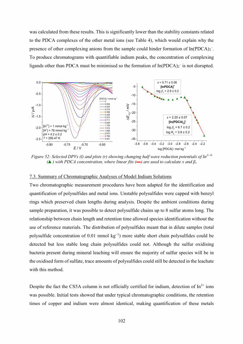
102

was calculated from these results. This is significantly lower than the stability constants related

to the PDCA complexes of the other metal ions (see Table 4), which would explain why the

presence of other complexing anions from the sample could hinder formation of In(PDCA)2–.

To produce chromatograms with quantifiable indium peaks, the concentration of complexing

ligands other than PDCA must be minimised so the formation of In(PDCA)2– is not disrupted.

-0.80 -0.75 -0.70 -0.65

-2.5

-2.0

-1.5

-1.0

-0.5

0.0

[In3+] = 1 mmol kg–1

[H+] = 76 mmol kg–1

pH = 4.2 ± 0.2T = 295.47 K

i /

A

E / V

[PDCA] / mmol kg–1

0 0.004 0.025 0.214 0.356 0.428 0.570 0.711 0.929 1.182 1.512 1.906 2.670 3.769 4.921

-3.8 -3.6 -3.4 -3.2 -3.0 -2.8 -2.6 -2.4 -2.2

-35

-30

-25

-20

-15

-10

-5

E

1/2 /

mV

log [PDCA] / mol kg–1

x = 0.71 ± 0.061

[InPDCA]+

log 1 = 2.9 ± 0.2

x = 2.20 ± 0.071

[In(PDCA)2]–

log 2 = 6.7 ± 0.2 log K2 = 3.8 ± 0.2

Figure 52: Selected DPVs (l) and plots (r) showing changing half wave reduction potentials of In3+/0

(▲) with PDCA concentration, where linear fits (▬) are used to calculate x and βx

7.3. Summary of Chromatographic Analyses of Model Indium Solutions

Two chromatographic measurement procedures have been adapted for the identification and

quantification of polysulfides and metal ions. Unstable polysulfides were capped with benzyl

rings which preserved chain lengths during analysis. Despite the ambient conditions during

sample preparation, it was possible to detect polysulfide chains up to 8 sulfur atoms long. The

relationship between chain length and retention time allowed species identification without the

use of reference materials. The distribution of polysulfides meant that in dilute samples (total

polysulfide concentration of 0.01 mmol kg−1) more stable short chain polysulfides could be

detected but less stable long chain polysulfides could not. Although the sulfur oxidising

bacteria present during mineral leaching will ensure the majority of sulfur species will be in

the oxidised form of sulfate, trace amounts of polysulfides could still be detected in the leachate

with this method.

Despite the fact the CS5A column is not officially certified for indium, detection of In3+ ions

was possible. Initial tests showed that under typical chromatographic conditions, the retention

times of copper and indium were almost identical, making quantification of these metals

103

impossible. It was possible to separate the elution of copper and indium by changing the

temperature at which these measurements were made and at 45 °C the peaks related to iron,

indium, copper, nickel, and zinc standards are well separated. Some adaptations to the

technique may be required to compensate for the complex background matrix of the leachates.

It was shown that the stability of the indium complex formed during chromatography is

significantly smaller than typical metal-PDCA complexes, hence the high concentration of

ligand ions in the leachate, i.e. sulfate, chloride, and nitrate, may interfere with the formation

of the In(PDCA)2– complex.

Techniques developed in this chapter will now be applied to project relevant solutions. The

chromatographic techniques to determine polysulfide and metal concentrations will be applied

to leaching samples. The experimentally determined stability constants have been collected in

the BHMZ database, so solution composition and properties can be included in geochemical

models to predict speciation and chemical behaviour of leachates and extraction solutions.

105

Table 9: Selected BHMZ contributing groups, aims, and collaborations during this work Group Aims Collaboration

2 Design, implementation, and operation of a research and testing in-situ bioleaching plant

- Provided mine water analysis (redox potential, pH, temperature)

6 The microbial leaching of target metal containing sphalerite

- Provided leachate samples from lab-scale leaching experiments

- Provided leachate analysis (ICP-MS, redox potential, pH, temperature)

- Leachate analysis with HPLC and IC to quantify polysulfide and metal ions

- Geochemical modelling of leachates with respect to pH, temp, redox potential

- Geochemical modelling of bioleaching efficiency

9

Development of a membrane separation process for selective recovery of metals from leaching solutions

- Provided membrane filtration samples

- Metal ion quantification in filtration samples with IC

- Geochemical modelling of various metal ions with respect to pH to explain metal retention during selective filtration

- Electrochemical determination of diffusion coefficients

12 Design electrolysis processes for the electrowinning and refining of indium

- Provided electrowinning electrolytes

- Determination of indium stability with electrowinning electrolytes

- Geochemical modelling of electrowinning samples

In the following chapter, analyses of three types of process relevant samples will be made.

Firstly in section 8, leachate solutions provided by group 6 who performed both in-situ and

laboratory scale bioleaching experiments will be investigated. The leaching solution applied to

ground ore in reactors (lab-scale) or directly to the ore body (in-situ) typically consisted of the

9K bacterial growth medium [Silverman and Lundgren 1959] in which a bacterial community

with Acidithiobacillus ferrivorans or Acidithiobacillus ferrooxidans as the major species was

cultivated. In addition FeSO4 was added and the solution acidified with H2SO4 [Gelhaar,

Schopf et al. 2015]. The goal of group 6 was to refine a leaching procedure that resulted in

leachates with an indium concentration of 10 mg L–1, as this was a viable concentration for the

subsequent indium extraction processes. In sections 8.1 and 8.2, chromatographic methods are

used to determine polysulfides and metal ion concentrations in leaching samples. Furthermore,

106

geochemical modelling is applied to predict speciation in the leachate, as well as the impact of

changing temperature, redox potential, and pH.

Membrane filtration samples were provided by group 9, who attempted to concentrate indium

in the leachate via selective filtration. Model solutions, for initial testing, as well as leachate

samples were passed over a filtration membrane with the goal to retain target metals in the

retentate, while undesirable metals e.g. iron, zinc, and copper passed through the membrane

into the permeate. In section 9 ion chromatography results are presented where the metal ion

concentrations in the retentate and permeate are determined. Geochemical modelling was used

to predict zinc, iron, copper, indium, and germanium speciation in these samples which offered

an explanation for the metal retention behaviour observed by group 9 with changing pH.

Figure 53 includes another indium concentration procedure: solvent extraction. During the

course of the BMHZ project, a successful solvent extraction procedure was developed. Indium

oxide with a purity of 99 % could be produced from complex solutions containing 1 mg L–1

indium and 1 g L–1 iron and zinc [Vostal, Šingliar et al. 2017]. Due to the organic solvents used

in this method, these solutions were not analysed in this work.

The final stage of the indium process chain, and the source of the third type of sample analysed

in this chapter, was the electrowinning and refining of indium. Two electrolyte systems were

suggested by group 12, based on methyl sulfonic acid (MSA) and methylglycinediacetic acid

(MGDA) respectively. In section 10 the DPV titration method (see section 5.1) was used to

determine the stability of indium with these electrolytes and hence geochemical modelling

could be used to determine the speciation of indium under the conditions of electrowinning.

8. Analysis of Leachate Solutions

8.1. Detection of Polysulfides in Leachate Solutions

The presence of sulfur oxidising bacteria in the leachate ensures that sulfate will be the most

prevalent sulfur species. However trace amounts of polysulfides are also expected. Following

the procedure developed for the polysulfide standard solutions (see section 7.1.1), leachates

were diluted in methanol and benzyl chloride was added to cap the polysulfide chains. The

resulting chromatograms from various leachates, compared to the 0.1 mmol kg−1 polysulfide

standard solution, are shown in Figure 54.

107

4 6 8 10 12 14 16

S8

Bz2S

coun

ts /

mA

U

t / min

0.1 mmol kg–1 polysulfide standard leachate 1 leachate 2 leachate 3 leachate 4 leachate 5 leachate 6

30 m

AU

Bz2S2

Bz2S3

Bz2S4

Bz2S5 Bz2S6

0 2 4 6 8 10

0

200

400

600

800

1000

1200

1400

tota

l pea

k ar

ea /

mA

U

total polysulfide concentration / mmol kg–1

R2 = 0.992

Figure 54: (l) Polysulfides found in leachates compared to the 0.1 mmol kg−1 standard solution (r) quasi-calibration curve using total polysulfide peak areas

Polysulfides could be detected in almost all leachate samples provided by group 6. It was

possible to detect polysulfides with chain lengths of up to 6 sulfur atoms and one leachate

showed presence of elemental sulfur. An additional peak at a retention time of 8.22 minutes

was found in samples 1 to 5 that could not currently be assigned. The procedure developed in

chapter two is not ideal for determining polysulfides at very low concentrations. Benzyl

chloride is insoluble in water, hence the leachate must be diluted in methanol which further

reduces polysulfide concentration. The concentration of benzyl chloride added must be

sufficient to induce rapid capping of polysulfides (to preserve distribution) but this results in a

large amount of benzyl chloride passing through the column. An alternative polysulfide

capping agent that does not have such a strong effect on the column could offer improved

results but this was not investigated in the scope of this work.

A quasi-calibration curve can be produced using the chromatograms of the standard polysulfide

solutions measured at different concentrations (see Figure 48). Unlike normal chromatographic

calibrations, where peak area with respect to the concentration of a single analyte is measured,

in this calibration the sum of all polysulfide peak areas, and hence total polysulfide

concentration, was considered. Using the calibration shown in Figure 54 (r), which showed a

linear relationship between total peak area and concentration, an average total polysulfide

concentration in the leachate samples of 12.5 µmol kg−1 can be estimated.

108

8.2. Determining Metal Ion Concentrations in Leachate Solutions

The aim of the measurements discussed in this section was to use the ion chromatography

methodology presented in section 7.2, to determine metal ion concentrations in leachate

samples. In the leachate, high iron and zinc concentrations were expected, depending on

column size, metal ion concentrations higher than 50 mg L–1, can permanently damage a

chromatographic column. An estimation of metal concentrations in the leachate was required

to determine a suitable leachate dilution factor. ICP-MS is a logical choice for such

measurements however standard addition with differential pulse voltammetry (DPV) can also

be used to analyse concentration as both peak height and area are proportional to concentration

(see equation 64). For initial testing with DPV a leachate dilution factor of 25 was used.

8.2.1. Leachate Metal Ion Quantification with DPV

Reduction of iron was not observed on the HMDE during DPV measurements, however a large

peak related to the Zn2+/0 redox couple can be seen in Figure 55 (l). The concentration of zinc

is significantly higher than the other metal ions, but redox potentials are sufficiently separated

so that the reduction of chromium, cadmium, and copper ions can also be observed. A variety

of leachate samples were analysed in this manner and some results are compared in Figure 55

(r), while presence of cadmium and copper occurred consistently in leachates, chromium and

lead could only be detected sporadically. At the time of these measurements, the goal of a

leachate sample with a indium concentration of 10 mg L–1, had not yet been achieved and

detection of indium was only possible in one leachate sample.

-1.0 -0.8 -0.6 -0.4 -0.2 0.0-0.8

-0.6

-0.4

-0.2

0.0

Cu2+/0

–0.026 V

Cd2+/0

–0.566 VCr3+/0

–0.797 V

i /

A

E / V

leachate 2

Zn2+/0

–0.977 V

-0.8 -0.6 -0.4 -0.2 0.0

leachate 1 leachate 2 leachate 3 leachate 4

In3+

i /

A

E / V

Cu2+Pb2+Cd2+Cr2+

0.02

A

Figure 55: (l) Typical leachate sample and (r) variations in trace metal components of leachates

measured with DPV (dilution factor 25)

109

The indium detection limit with DPV is around ten times lower than in IC measurements

(ca. 0.01 mg L–1 with DPV compared to 0.1 mg L–1 with IC), and the DPV detection limit can

be further reduced when anodic stripping voltammetry is employed to concentrate indium on

the mercury drop electrode (concentration of 10–5 mg L–1 could be detected). However the

similarities between the reduction potentials of cadmium and indium, and hence overlapping

peaks, meant quantification of indium in these measurements was not possible, (see Figure 56).

Standard addition was used to determine the concentrations of metal ions in the leachate during

DPV measurements. Due to the differing concentrations of zinc, cadmium, and copper in

comparison to the trace concentrations of lead and indium, two standard addition protocols

were prepared. Figure 56 (l) shows the results of a simultaneous standard addition of zinc,

cadmium, and copper, and Figure 56 (r) shows the addition of indium and lead.

-1.2 -1.0 -0.8 -0.6 -0.4 -0.2 0.0-3.0

-2.5

-2.0

-1.5

-1.0

-0.5

0.0

0.0 0.2 0.4 0.6 0.8 1.00123

456

leachate 3

Cu2+Cd2+Zn2+

i /

A

E / V

a)

Cu2+

Pb2+In3+

Cd2+

[Cd2+] = 0.2 ± 0.5 mg L–1

ICP-MS = 0.15 mg L–1

[Cu2+] = 0.8 ± 0.5 mg L–1 ICP-MS = 0.22 mg L–1

peak

are

a / n

AV–1

concentration added / mg L–1

-0.7 -0.6 -0.5 -0.4 -0.3 -0.2 -0.1

-0.03

-0.02

-0.01

0.00

0.0 0.2 0.4 0.6 0.8 1.0-15

-10

-5

0

leachate 3

In3+

Pb2+

Cd2+

In3+

i /

A

E / V

a) [Pb2+] = 0.06 ± 0.1 mg L–1

ICP-MS = 0.049 mg L–1

i p /

nA

concentration added / mg L–1

Figure 56: Standard addition of (l) zinc, cadmium, and copper using peak areas and

(r) indium and lead using peak heights to determine metal concentrations in leachates

In the DPV measurements of leachate sample 3, it initially appeared that the cadmium and

indium peaks would be sufficiently separated to allow quantification with standard addition.

However, with the addition of indium standards it became impossible to resolve two distinct

peaks for indium and cadmium. Indium peak heights could only be determined when indium

peaks surpassed the cadmium peaks. Hence, it was not possible to accurately determine indium

concentration with standard addition as the error was too large. Standard addition with DPV is

not a suitable method to quantify indium concentration in cadmium containing leachates.

Other leachate components could be more successfully analysed. The concentrations of zinc,

cadmium, copper, and lead determined with standard addition were in good agreement with

110

values determined by ICP-MS: [Zn2+] = 58.0 ± 3.7 mg L–1 (ICP-MS 55.45 mg L–1),

[Cd2+] = 0.2 ± 0.5 mg L–1 (ICP-MS 0.15 mg L–1), [Cu2+] = 0.8 ± 0.5 mg L–1 (ICP-MS

0.22 mg L–1), and [Pb2+] = 0.06 ± 0.1 mg L–1 (ICP-MS 0.049 mg L–1). As none of these metal

concentrations exceeds the limit of 50 mg L–1, these samples would be suitable for IC

measurements. Depending on the component concentrations, leachates will have to be diluted

by a factor of 25 to 50 before quantification with ion chromatography.

8.2.2. Leachate Metal Ion Quantification with Ion Chromatography

Separation of multi-element standard solutions was proven effective at a raised column

temperature of 45 °C in PDCA eluent (see section 7.2). Measurements of leachates would be

complicated by i) large differences between metal ion concentrations, and ii) leachate anions

which could contribute to matrix effects on the column. The following section will discuss the

adaption of the IC technique for successful quantitative leachate analysis.

Due to the high iron and zinc concentrations which would overload the column, the leachate

was diluted in water before measurement. Unfortunately the concentration of indium in the

leachate after dilution (0.002 mg L–1 determined with ICP-MS) was not sufficient to be

detected with IC. The detection limit of indium in these IC measurements was determined with

increasingly dilute indium standards, while peaks relating to indium concentrations of less than

0.5 mg L–1 could be seen, the signal to noise ratio required concentrations of close to 1 mg L–1

for accurate quantification. To show that IC would be a suitable technique for leachate

quantification when the 10 mg L–1 indium concentration target is reached, small amounts of an

indium standard solution was added to the leachates. This resulted in two rather one additional

peak appearing in the chromatogram (see Figure 57).

Several indium standard solutions were prepared from various sources to rule out

contamination, but results were reproducible. It was considered that the peak was a result of

indium redox chemistry, In+ can be stable under certain conditions, but measurements in an

oxidising media (H2O2) only effected the ratio of ferrous and ferric iron. Once all other

alternatives had been rules out, it was concluded that the second additional peak was caused by

indium peak splitting due to high concentrations of complexing ligands in the leachate, most

likely sulfate, which inhibited formation of the In(PDCA)2– complex in the eluent (see section

7.2.2).

111

4 6 8 10 12 14

0

200

400

600

800

1000

Leachate + 3 mg L–1 In3+

+ 5 mg L–1 In3+

Leachate 1 diluted in H2O

45 oCcoun

ts /

mAU

t / min

Fe3+

?In3+

Cu2+

Ni2+

Zn2+

Mn2+

Fe2+ 5.5 6.0 6.5

50

100

150

coun

ts /

mAU

t / min

?

In3+ - 6

.18

Figure 57: Chromatograms of the indium doped leachate resulting in an additional unidentified peak

In an attempt to minimise competing ligand effects during interactions between the sample and

the mobile phase, leachate samples were diluted in PDCA rather than water. Chromatograms

showing a single peak with addition of indium standards can be seen in Figure 58. Separation

of the peaks means concentrations of ferric and ferrous iron, indium, copper, nickel, zinc, and

manganese can be successfully quantified (see Table 10) in a single measurement.

Table 10: Concentrations of selected leachate components determined by ICP-MS and IC

2 4 6 8 10 12 14 160

200

400

600

800

1000

1200

1400

In3+

Leachate 1 diluted in PDCA

45 oC

coun

ts /

mAU

t / min

Leachate + 1 mg L–1 In3+

+ 3 mg L–1 In3+

+ 5 mg L–1 In3+

Fe3+

In3+

Cu2+

Ni2+

Zn2+

Mn2+

Fe2+

5.75 6.00 6.25 6.500

25

50

75

100

125

coun

ts /

mAU

t / min

4.90(3) mg L–1

3.17(2) mg L–1

0.91(7) mg L–1

In3+ conc.

Concentration

mg L–1 ICP-MS IC

Fe3+ 45

31.67(3)

Fe2+ 17.56(4)

Zn2+ 13.6 13.48(1)

Ni2+ 1.70 2.05(1)

Mn2+ 1.01 1.07(1)

Cu2+ 0.11 0.06(3)

In3+ 0.002 <0.1

Figure 58: Chromatograms of the leachate diluted with PDCA with addition of indium standards

As expected, concentrations of iron and zinc exceeded all other metals. The source of zinc in

the leachate is solely from the oxidation of sphalerite, however presence of iron in the leachate

is the results of mineral oxidation (pyrite, chalcopyrite) but also the initial addition of FeSO4

112

to the leaching solution. After one day almost all ferrous iron had been oxidised, this process

could be slowed by degassing the sample and pre-treating the CS5A column with 0.1 mol kg−1

Na2SO3 to remove oxygen, but not halted indefinitely. The lower concentrations of copper,

indium, nickel, and manganese are likely from their inclusion in mineral phases via ionic

substitution.

It was not possible to quantify every metal ion present in leachate samples with ion

chromatography, either because concentrations were below detection limits, or detection was

not possible with the CS5A column and PDCA eluent (e.g. lead). It was however possible to

simply and quickly determine the concentrations of a number of metal ions simultaneously,

and unlike in ICP-MS methods it was possible to differentiate between ferric and ferrous iron

which is essential when investigating the behaviour of iron oxidising bacteria.

The development of this technique resulted in a previously unknown functionality of the CS5A

column. While indium concentrations in the supplied leachates are currently below the

detection limits, leachates diluted in PDCA to minimise sample-mobile phase interactions,

would result in chromatograms suitable for leachate quantification when the 10 mg L–1 target

indium concentration is reached.

8.3. Geochemical Modelling of Leachate Solutions

Complex stability constants determined in section 5 were included in the BHMZ database. In

section 6, speciation of indium in model solutions (i.e. with addition of a single complexing

ligand or increasing pH) was predicted using geochemical modelling. For certain sample

conditions, such a temperature and redox potential, when no value is given by the user,

PHREEQC uses default values. While this was acceptable in the PHREEQC input files

describing the simple models, these values would have to be determined for accurate

geochemical modelling of leachates. Initial leaching investigations performed by group 6 in

the laboratory yielded very consistent results regarding leachate pH (typically pH 1 to 2),

temperature (measurements were made at 30 ºC), and redox potential (typically 600 to

800 mV). In in-situ bioleaching, factors such as the presence of multiple mineral phases, and

lower underground temperatures, will likely result in more variable leachate conditions.

Naturally occurring bacterial oxidation of minerals is constantly occurring in the mine. Acid

mine drainage (AMD) occurs when the mine waters resulting from uncontrolled bioleaching

114

water analysis in Table 11 will provide the pH, redox potential, and temperature limits for the

models.

8.3.2. Geochemical Modelling of a Leachate Solution

A thorough analysis of a laboratory leachate sample was made: ICP-OES, ICP-MS and IC were

used to determine sample composition, additionally redox potential (769 mV vs. SHE), pH

(1.69), and temperature (25 °C) were measured. PHREEQC required 9 iterations to produce a

model of the leachate with an error of 1.34 % using the BHMZ database (for the PHREEQC

input file see Appendix ii.v). Selected predictions of the model are given in Table 12.

Component concentrations (listed in decreasing order) were determined in mg L–1 and results

of the geochemical model was given in mol kg−1, hence the total concentrations of selected

leachate components are given in both forms in Table 12. Additionally, the species found at

significant concentrations for each component, as well as the percentage at which these are

found (with respect to each individual component) is shown in Table 12. For example,

7930 mg L–1 (or 8.344 × 10–2 mol kg−1) of sulfate ions were detected in the leachate, the model

predicted the major sulfate species were SO42– and HSO4

– and 53.70 % of total sulfate was in

the form SO42– and 27.30 % in the form HSO4

– (remaining sulfate was in the form of metal

sulfate complexes).

For most metals, the predominant species in the leachate was either the free cation or a sulfate

complex. However due to the high sulfate concentration, only 19 % of the total sulphate

concentration was complexed. This is compared to 2.26 and 2.29 % of chloride and nitrate

concentrations respectively. No nitrate complexes were predicted by the model at substantial

amounts and only indium and cadmium had chloride complexes at any significant

concentrations. Although the redox potential is relatively high (769 mV), the low pH (pH 1.69)

means both ferric and ferrous iron are stable. The ratio of sulfate to hydrogen sulfate

([SO42–] > [HSO4

–]) is consistent with the pH, and pKa values of sulfuric acid. From the

saturation indicies (see section 3.6), the model predicted the phases at equilibrium (–

1 ≤ SI ≤ 1): anglesite (PbSO4), goethite (FeOOH), gypsum (CaSO4·2 H2O), and jarosite

(KFe3(SO4)2(OH)6). As well as saturated phases (SI ≥ 1): hematite (Fe2O3).

115

Table 12: Speciation analysis of a leachate sample predicted by PHREEQC

Total Concentration

Measured mg L–1

Modelled mol kg−1

Significant Speciation %

SO42– 7930 8.344 × 10–2 SO4

2–

HSO4–

53.70 27.30

Zn 1410 2.179 × 10–2 Zn2+ ZnSO4

59.52 40.49

Fe3+ 904

8.896 × 10–3 Fe3+

FeOH2+

FeSO4+

69.31 11.78 9.54

Fe2+ 7.463× 10–3 Fe2+ FeSO4

58.17 41.82

Mg 76.9 3.198 × 10–3 Mg2+ MgSO4

52.35 47.62

Ca 56.6 1.427 × 10–3 Ca2+ CaSO4

64.16 35.76

Mn 37.6 6.917 × 10–4 Mn2+ MnSO4

53.49 46.45

Cl– 26.8 7.640 × 10–4 Cl– 97.53

Cd 12.9 1.160 × 10–4 Cd2+

CdCl+ 89.74 9.88

NO3– 12.1 8.730 × 10–4 NO3

– 97.71

Cu 9.47 1.506 × 10–4 CuSO4 Cu2+

50.00 49.73

As 4.07 5.490 × 10–5 H3AsO4 H2AsO4

– 69.16 30.84

Ni 0.809 1.393 × 10–5 Ni2+ NiSO4

63.25 36.70

Al 0.614 2.300 × 10–5 Al(SO4)2

–

AlSO4+

Al3+

42.32 41.47 16.20

K 0.5 1.292 × 10–5 K+

KSO4–

91.41 8.57

Cr 0.477 4.157 × 10–6 Cr3+ 99.73

Pb 0.421 2.053 × 10–6 Pb2+ 99.03

In 0.269 2.368 × 10–6 In3+

InSO4+

InCl2+

88.98 7.15 2.98

116

It was not possible to determine stability constants for the metastable polysulfide species.

However other sulfur species could be modelled using the Lawrence Livermore National

Library (LLNL) database [Johnson, Anderson et al. 2000], which includes reliable data for a

wide variety of minerals and aqueous species [Blasco, Gimeno et al. 2017]. Figure 60 (l) shows

a Pourbaix diagram for the aqueous sulfur species produced using Phreeplot and the LLNL

database (for an example of a Phreeplot input file for a Pourbaix diagram see Appendix ii.vii).

Due to its stability, SO42– is the dominant species over a wide range of potentials and pH values.

At strongly acidic pH values below pH 2, where H2SO4 is only partially dissociated, the

concentration of HSO4– exceeds SO4

2–. At low redox potentials below 250 to –250 mV

(depending on pH) H2S is the predominant species but at neutral pH values it is deprotonated

to HS–.

Figure 60: Pourbaix diagrams showing (l) predominant sulfur species in the leachate and

(r) aqueous sulfur species when SO42– formation is supressed [Druschel, Hamers et al. 2003]

As a Pourbaix diagram defines the predominant species at various pH and redox potentials, the

distribution of minor sulfur species is not described. One method to observe these species in

the model is to supress the formation of the predominant sulfate species. In the plot produced

by [Druschel, Hamers et al. 2003] shown in Figure 60 (r), it was possible to observe species

such as thiosulfate (S2O32–) and polythionates (SxO6

2–). Although supressing the formation of

such a significant species would have a substantial effect on the remaining sulfur species, and

hence brings the validity of the resulting model into question.

117

8.3.3. Modelling of Leachate Solutions at various pH, Redox Potentials, and Temperatures

Due to the results of the mine water analysis in section 8.3.1, the previously modelled

laboratory leachate sample was examined over a wider range of properties: pH 0 to 7, redox

potential –0.1 to 1.1 V, and temperature 9 to 20 °C.

pH Value

The dominant species, and the pH at which the predominant species changes, are shown in the

predominance plot in Figure 61. At low pH values, the majority of ions are un-complexed, and

as pH increases hydrolysis or sulfate complexes are formed. While the presence of iron and

indium sulfate complexes are predicted by the model, they are at low concentrations. At high

pH values iron and indium form hydroxide complexes, the low concentration of indium means

the neutral hydroxide In(OH)3 remains soluble, however most of the iron is precipitated as

Fe(OH)3 (s). Precipitation of iron containing phases are also seen with other ions: magnesium,

calcium, copper, and nickel are precipitated as ferrites and potassium as jarosite. The high

concentration of zinc ensures that while zinc ferrite (ZnFe2O4) is also formed, the amount of

soluble ZnSO4 exceeds that of the precipitate. Both manganese and aluminium form sulfate

complexes before precipitation of pyrolusite and diaspore respectively. At neutral pH arsenic

precipitation as lammerite is predicted. Cadmium remain un-complexed throughout the entire

pH range, lead does not form complexes but at higher pH values, is precipitated as crocoite.

Chromium form soluble oxide complexes that become deprotonated with increasing pH.

At neutral pH the model predicts there are over 40 additional mineral phases that are either at

equilibrium or saturated. Many ferric phases have a positive SI which is to be expected from

the insolubility of ferric iron at high pH values: delafossite (CuFeO2), geothite (FeOOH),

hematite (Fe2O3), magnetite (Fe3O4), and trevorite (NiFe2O4). Additionally, many manganese

phases are saturated: birnessite (Mn8O14·5 H2O), todorokite (Mn7O12·5 H2O), bixbyite

(Mn2O3), hausmannite (Mn3O4), and manganite (MnO(OH)). Copper mineral phases:

brochantite (Cu4(SO4)(OH)6), antlerite (Cu3(SO4)(OH)4), atacamite (Cu4Cl2(OH)6), and

tenorite (CuO). Furthermore, the following saturated aluminium phases: boehmite (AlO2H),

gibbsite (Al(OH)3), corundum (Al2O3), and alunite (KAl3(OH)6(SO4)2).

118

0 1 2 3 4 5 6 7

PbCrO4 (s)

5.50

KFe3(SO4)2(OH)6 (s)

1.78AlHO2 (s)

NiFe2O4 (s)

3.17Cu3(AsO4)2 (s)

6.64CuFe2O4 (s)

3.11

MnO2 (s)

5.44CaFe2O4 (s)

MgFe2O4 (s)

5.31

CrO42–

HAsO42–

Fe(OH)3 (s)

6.184.03

4.99

6.402.39

1.95

1.84

5.12

1.58

4.40

2.13

pH

In

Pb

Cr

K

Al

Ni

As

Cu

Cd

Mn

Ca

Mg

Fe

Zn2.53 3.44 4.20

1.16 1.95

4.43 4.75

Zn2+ ZnSO4

Fe3+FeOH2+

Fe3(OH)45+

Fe(OH)2+

Mg2+ MgSO4

Ca2+

Mn2+ MnSO4

Cd2+

Cu2+ CuSO4

H3AsO4H2AsO4

–

Ni2+

Al3+ AlSO4+ Al(SO4)2

–

K+

Cr3+ HCrO4–

Pb2+

In3+ In(OH)2+ In(OH)3

Figure 61: Dominant speciation of metal ions in the leachate between pH 0 and 7

Redox Potential

As mentioned in section 3.6.1, in PHREEQC the redox potential of a solution is defined by the

function ‘pe’, where pe is the negative logarithm of electron activity. The relationship between

redox potential, E, and pe is –log{e–}a = 16.9 × E. Hence, when the leachate described in

section 8.3.2 was modelled between pe –2 and 19, this correlated to redox potentials between

–0.12 and 1.12 V.

Only the speciation of redox active metals would be affected by changes in redox potential. Of

all the redox couples considered in the model, As3–/3+/5+, Cr2+/3+/5+/6+, Cu+/2+, Fe2+/3+, In+/3+,

Mn2+/3+/6+/7+, Pb2+/4+, only copper and iron speciation showed significant changes with respect

to redox potential. Below E = 0.764 V, the predominate iron species was Fe2+, and above this

potential, Fe3+. This is consistent with the standard redox potential of the Fe3+/2+ couple

Eϴ = 0.771 V [Bard and Parsons 1985]. Below 0.586 V the dominant copper species was

CuCl32– and at higher potentials CuSO4 (aq) (but Cu2+ was at almost the same concentration).

This is similar to the redox potential related to CuCl ⇌ Cu2+ found in the literature where

119

Eϴ = 0.537 V [Bard and Parsons 1985]. Due to the iron oxidising bacteria in the leachate

maintaining a high ferric iron concentration, the redox potential of leachate samples will

normally be relatively high, hence metal ions in the leachate will be in their oxidised state.

At low redox potentials, the model predicts arsenic has a positive saturation index, anglesite

(PbSO4), Cu, anhydrite (CaSO4), and gypsum (CaSO4·2 H2O) are at equilibrium. At high redox

potentials the saturated phases are: hematite (Fe2O3), jarosite (KFe3(SO4)2(OH)6), and goethite

(FeOOH). Pyrolusite (MnO2), anglesite (PbSO4), and gypsum (CaSO4·2 H2O) are at

equilibrium.

Temperature

The same procedure was used to model the leachate described in section 8.3.2 at temperatures

between 9 to 20 °C. Temperature did not have a significant effect on speciation but in general,

the concentration of sulfate complexes increased slightly and free metal ion concentrations

decreased, with increasing temperature. When precipitation is observed in the leachate at

higher pH values, temperature would have an impact on the solubility of these solid phases,

although over a temperature range of 10 °C, it is likely that this effect is also small.

8.3.4. Geochemical Modelling of Bioleaching Efficiency

Geochemical models cannot consider the behaviour and activity of bacteria, however an abiotic

leaching process could be modelled with some simplifications. If a geochemical model is

designed such that the modelled parameters are as similar as possible to an experimental

bioleaching process, the difference between the predictions of the abiotic model and the

experimental bioleaching results could be attributed to bacterial effects.

The parameters for the model came from bioleaching experiments carried out by BHMZ

colleagues from group 6 [Gelhaar, Schopf et al. 2015]: the experimental bioleaching solution

consisted of the 9K bacterial growth medium [Silverman and Lundgren 1959] containing

3 g L–1 (NH4)SO4, 0.1 g L–1 KCl, 0.5 g L–1 K2HPO4, 0.5 g L–1 MgSO4·7H2O, and 0.01 g L–1

Ca(NO3)2. In addition, 72 mmol kg−1 FeSO4 was added and the solution acidified to pH 2.70.

A bacterial community with Acidithiobacillus ferrivorans as the major species was cultivated

in this medium and 2 mass % of ground mineral ore (containing roughly 30 % sphalerite, 30 %

pyrite, 20 % galena, and 20 % quartz) was added to the leaching solution. After 20 days the

leachate had a pH of 1.8 and a redox potential of 850 mV and the zinc recovery rate was 70 %.

120

In the geochemical model the basis consisted of a solution with the same elemental

composition, pH, and temperature as the experimental bioleaching solution. This solution was

equilibrated with CO2 (g), O2 (g), and solid phases the same as the ore composition from the

experimental measurements. After equilibration, the model predicted the solution would have

a pH of 2.49 and a redox potential of 181 mV, the predicted zinc concentration in solution

would be equivalent to a zinc recovery rate of 50 %. The PHREEQC input file for this model

can be found in Appendix ii.vi.

The differences between the predictions of the model and the results of the bioleaching

experiments could be attributed to bacterial activity. Without the liberation of protons by sulfur

oxidising bacteria (equations 7 to 10) in bioleaching, the pH predicted by the model would be

higher than the one measured in the bioleaching experiment. Additionally the model cannot

consider iron oxidising bacteria (equation 11) present in the experimental bioleaching

measurements, therefore ferrous iron is not re-oxidised in the model and hence the predicted

redox potential is much lower. The lower concentrations of protons and ferric iron considered

by the model mean the oxidation rate of sphalerite would be significantly decreased and

therefore the predicted zinc concentration in solution was much lower. The comparison

between experimental results and the predictions of the model are summarised in Table 13.

Table 13: Selected experimental results and predictions from a

geochemical model attempting to replicate the bioleaching experiment Bioleaching

experiment Abiotic model

pH 1.8 2.49

Redox / mV 850 181

Zinc yield / % 70 50

Assuming an accurate model, the differences between the values listen in Table 13 could be

attributed to the bacterial activity not considered by the geochemical model, but realistically

this could be an oversimplification and requires experimental verification. As well as bacterial

effects, the model did not consider kinetic effects during the bioleaching experiments, for

example stirring and the increased mineral surface area of ground ore. Additionally, as the

model does not consider the bacterial oxidation of ferrous iron, the lack of ferric iron in the

modelled leachate means no precipitation of jarosite or iron hydroxide is predicted which is

not consistent with the experimental results. Since such precipitates usually form layers that

121

cover the mineral surface and inhibit oxidative attack, this is a significant difference between

the modelled and the actual experimental conditions. To more accurately quantify the effect of

bacterial activity on sulfidic mineral leaching, an experimental rather than theoretical

comparison between biotic and abiotic measurements is required. The results of an

experimental abiotic leaching measurement could be compared to this model, verification that

the predictions of this model are true, could allow this model to be used in further simulations.

8.4. Application of Analysis Methods to Leachate Solutions

A number of the techniques developed in the initial stages of this work were applied to leachate

samples provided by group 2 (see Table 9). Using chromatographic methods it was possible to

estimate an average total polysulfide concentration of 12.5 µmol kg−1 in leachate samples.

Due to a combination of the high concentration of complexing ligands in the leachate, and the

relatively low stability (in comparison to other metals) of the PDCA complex formed in the IC

eluent, the IC technique for quantifying metals had to be adapted for leachate analysis. When

leachate samples were diluted with PDCA instead of water, concentrations of iron, copper,

nickel, zinc, and manganese could be determined simultaneously. When the target leachate

indium concentration of 10 mg L–1 is reached, this technique will also be applicable for the

quantitative determination of indium.

The predominant speciation, and the effect that pH, redox potential, and temperature had on

leachate speciation was predicted with geochemical modelling. Additionally, a geochemical

model describing an experimental bioleaching process was constructed. If the predictions of

the model could be experimentally verified, the model could be used to theoretically quantify

the effects of bacterial activity during leaching.

122

9. Analysis of Membrane Filtration Solutions

One of the proposed stages of the indium extraction process is the concentration of target metals

in solution with selective filtration. A feed solution passes through or over a filtration

membrane where target metals remain in the retentate and other metals pass through to the

permeate solution. The speciation of indium, especially regarding the charge and size of the

complex, is essential for both membrane design and to understand metal interaction with the

membrane. Listed in Table 14 is the classes of filter membranes divided according to pore size.

As described in Figure 53, various sequential filtration processes will be required for the

extraction of indium from leaching solutions.

Table 14: Various filtration process defined by filter pore size [Melin and Rautenbach 2003]

Pore size / nm

Molecular mass / kDa Process Pressure /

bar Filtration

< 1 < 0.1 reverse osmosis 10 – 80 salts, small organic molecules

1 – 2 0.1 – 5 nanofiltration 3 – 20 poly/monovalent ions

2 – 100 5 – 5000 ultrafiltration 1 – 10 macromolecules, proteins

> 100 > 5000 microfiltration < 2 particles

> 10 µm - classic filtration - bulk solids

In the following section, ion chromatography will be used to determine the metal ion

concentrations in retentate and permeate solutions to investigate the selective filtration of

model solutions. Furthermore, geochemical modelling will be used to explain the retention

behaviour observed by group 9, during membrane filtration experiments made at various pH

values. To understand the interactions between the membrane surface and species in solution,

both particle size and charge are important parameters. The speciation, and hence charge, can

be predicted with geochemical modeling and the respective hydrodynamic radii can be

calculated from diffusion coefficients. In the final part of this section various electrochemical

methods are presented for the determination of indium diffusion coefficients.

9.1. Determining Metal Ion Concentrations in Membrane Filtration Solutions

Before membrane filtration methods could be applied to leachate samples, investigations using

model solutions containing metal ions found in the leachate were made by group 9 (see Table

123

9). Samples containing 0.1, 0.5, and 1 mmol kg−1 iron, indium, copper, zinc, and germanium

underwent a cross-flow filtration experiments at various pH values using a polyethersulfone-

based membrane filter, NP010. The aim of these investigations was to find filtration conditions

that selectively increased the concentration of target metals in the retentate. The concentrations

of metals ions in the retentate and permeate were determined with IC and compared to the

results of previous ICP-MS analysis. Figure 62 shows chromatograms of the retentate and

permeate after a 0.1 mmol kg−1 sample was filtered at pH 1.7. The concentrations determined

with IC and ICP-MS are shown in Table 15.

Table 15: Concentrations in the retentate and permeate determined by ICP-MS and IC

0 2 4 6 8 10 12 14

0

100

200

300

400

500

600

45 oC

In3+

retentate permeate

coun

ts /

mA

U

t / min

Fe3+

Cu2+ Zn2+

Fe2+

Retentate mg L–1

Permeate mg L–1

ICP-MS IC ICP-

MS IC

Fe3+ 5.61

4.16 3.86

2.74

Fe2+ 1.32 0.97

In3+ 16.3 19.1 7.44 14.5

Cu2+ 9.54 8.84 5.17 6.12

Zn2+ 7.60 10.95 6.66 7.68

Ge4+ 4.50 - 3.04 -

Figure 62: Chromatograms of the retentate and permeate after membrane filtration

As previously established in section 7.2, due to the similarities in the retention times of In3+

and Cu2+ on the CS5A column, separation of the peaks related to indium and copper requires

chromatograms to be measured at 45 °C. While the separation of copper and indium retention

times in the membrane filtration samples was successful, quantification of germanium was not

possible.

Normally the sample that is injected into the eluent contains hydrated or weakly complexed

metal ions. This means ligands in the sample can be easily displaced by eluent complexing

agents such as PDCA, and formation of the required metal-PDCA complex occurs without

difficulty. The formation of germanic acid (H4GeO4) in aqueous solutions, rather than cationic

Ge4+, likely means the formation of a Ge-PDCA complex does not occur. Hence,

chromatographic determination of germanium is not possible with the available setup.

124

Quantification of indium, copper, zinc, and iron was possible in these measurements, and

higher concentrations could be found in the retentate than in the permeate, however at pH 1.7

filtration was unselective as concentrations of all metal ions increased.

9.2. Geochemical Modelling of Membrane Filtration Solutions

In an attempt to find a pH at which the selective filtration of indium could occur, group 9 of

the BHMZ, performed a series of membrane filtration measurements using 0.1 mmol kg−1

model solutions at various pH values. The retention of the respective metal ions was calculated

from the ratio of the metal ion concentrations found in the permeate and retentate using

equation 88. A plot of retention with respect to pH for indium, germanium, zinc, and copper

can be seen in Figure 63.

𝑅 = (1 −[M]𝑝𝑒𝑟𝑚𝑒𝑎𝑡𝑒

[M]𝑟𝑒𝑡𝑒𝑛𝑡𝑎𝑡𝑒) (88)

0 2 4 6 8 10 12

0

20

40

60

80

100

In Ge Zn Cu

Ret

entio

n / %

pH

[M] = 0.1 mmol kg–1

Figure 63: Retention of indium, germanium, copper, and zinc at various pH values after filtration of a

0.1 mmol kg−1 model solution with a nanofiltration polymer membrane

A significant increase in the retention of indium occurs above pH 5, and the retention of copper

and zinc above pH 8. As speciation, both with regard to size and charge, would have a

significant impact on interactions with the membrane surface, and hence retention behaviour,

speciation of the metals in the model solutions were modelled with respect to pH. A pH range

between 0 and 14 was used and temperature and redox potential were kept constant at the

default program values (25 °C, pe = 4 or 237 mV). A redox potential between 100 and 300 mV

125

is realistic for dilute aqueous systems [Goncharuk, Bagrii et al. 2010]. The speciation of zinc,

copper, and germanium in 0.1 mmol kg−1 solutions at increasing pH values are shown in Figure

64. The speciation of 0.1 mmol kg−1 indium under the same conditions has been presented

previously in Figure 41 (l). At an indium concentration of 0.1 mmol kg−1, unlike in the

analogous zinc and copper results, no precipitation of In(OH)3 (s) is predicted. Additionally no

formation of polynuclear indium species is expected.

In Figure 64 (top) formation of the first zinc hydroxide complex ZnOH+ begins at pH 6, this is

much later than indium where formation of InOH2+ is already occurring at pH 2. Hydrolysis of

Cu2+ also begins at pH 6, Cu+ is found in small concentrations below pH 7. Initially both zinc

and copper form positively charged mono-hydroxide complexes, as pH increases neutral

hydroxides are precipitated, and eventually negatively charged complexes are formed at very

high pH. A change in complex charge would have a significant effect on the interactions

between metal and membrane. Precipitation of neutral hydroxides would result in the

membrane filter acting as a physical barrier between the retentate and permeate, however issues

of un-selectivity and membrane fouling could arise. At a concentration of 0.1 mmol kg−1, no

precipitation of germanium hydroxide is expected, the deprotonation of germanic acid occurs

above pH 9.

The results of the geochemical model shown in Figure 41 (l) predicts soluble indium hydroxide

species at a concentration of 0.1 mmol kg−1. However membrane filtration is being used a

method to concentrate indium in solution, ideally indium concentrations will not remain so

low. The solubility of In(OH)3 (aq) predicted in section 6.2 is 0.508(1) mmol kg−1 (see Figure

43) and above this concentration, issues of indium hydroxide precipitation, i.e. membrane

fouling, must be considered.

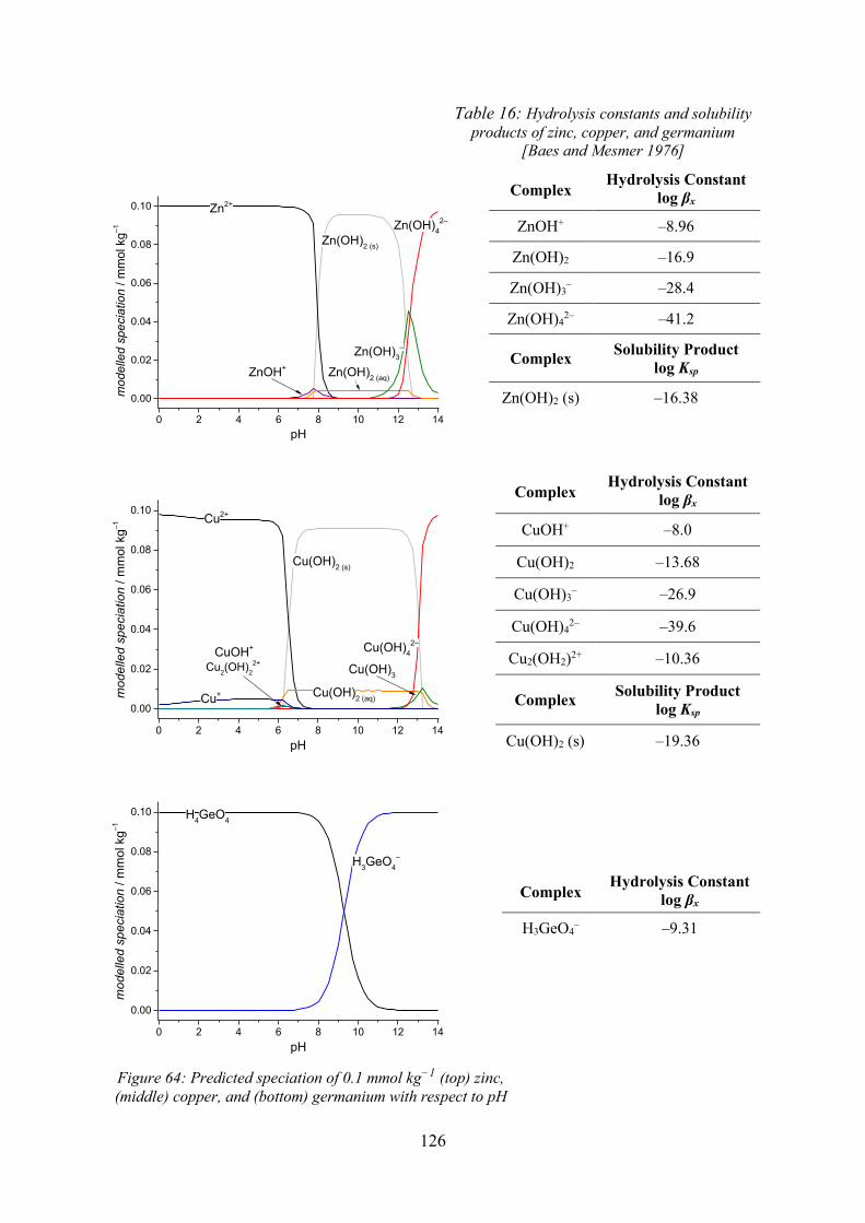
126

Table 16: Hydrolysis constants and solubility products of zinc, copper, and germanium

[Baes and Mesmer 1976]

0 2 4 6 8 10 12 14

0.00

0.02

0.04

0.06

0.08

0.10

Zn(OH)2 (aq)

mod

elle

d sp

ecia

tion

/ mm

ol k

g–1

pH

Zn2+

ZnOH+

Zn(OH)3–

Zn(OH)2 (s)

Zn(OH)42–

Complex Hydrolysis Constant

log βx

ZnOH+ –8.96

Zn(OH)2 –16.9

Zn(OH)3– –28.4

Zn(OH)42– –41.2

Complex Solubility Product log Ksp

Zn(OH)2 (s) –16.38

0 2 4 6 8 10 12 14

0.00

0.02

0.04

0.06

0.08

0.10

Cu2(OH)22+

CuOH+

mod

elle

d sp

ecia

tion

/ mm

ol k

g–1

pH

Cu2+

Cu+ Cu(OH)2 (aq)

Cu(OH)3

Cu(OH)42–

Cu(OH)2 (s)

Complex Hydrolysis Constant

log βx

CuOH+ –8.0

Cu(OH)2 –13.68

Cu(OH)3– –26.9

Cu(OH)42– –39.6

Cu2(OH2)2+ –10.36

Complex Solubility Product log Ksp

Cu(OH)2 (s) –19.36

0 2 4 6 8 10 12 14

0.00

0.02

0.04

0.06

0.08

0.10

H3GeO4–

H4GeO4

mod

elle

d sp

ecia

tion

/ mm

ol k

g–1

pH

Complex Hydrolysis Constant

log βx

H3GeO4– –9.31

Figure 64: Predicted speciation of 0.1 mmol kg−1 (top) zinc, (middle) copper, and (bottom) germanium with respect to pH

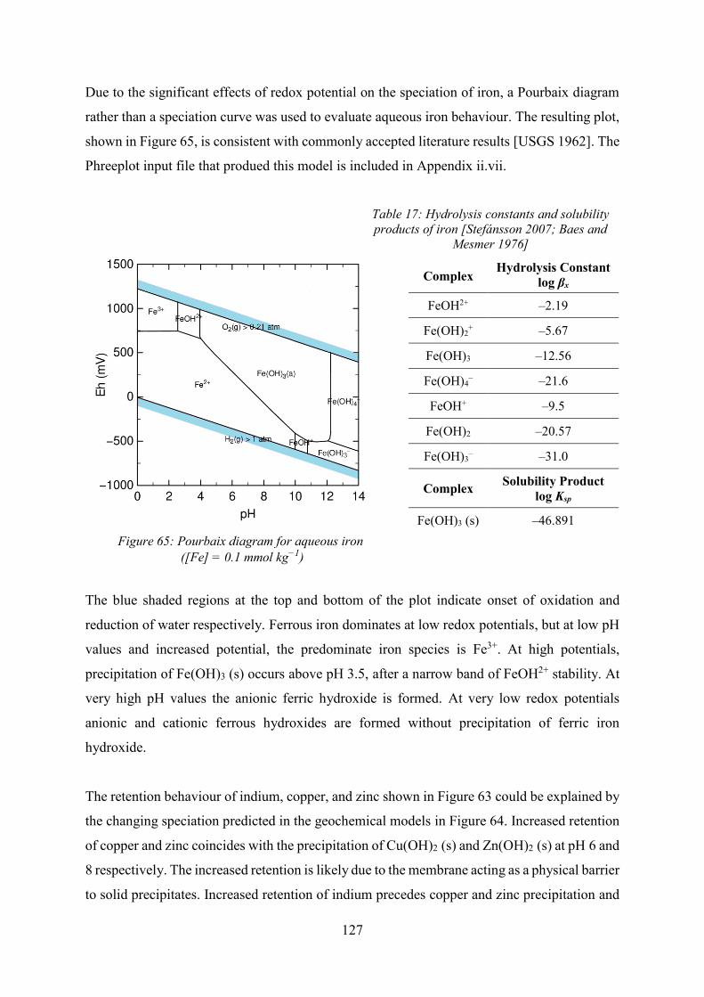
127

Due to the significant effects of redox potential on the speciation of iron, a Pourbaix diagram

rather than a speciation curve was used to evaluate aqueous iron behaviour. The resulting plot,

shown in Figure 65, is consistent with commonly accepted literature results [USGS 1962]. The

Phreeplot input file that produed this model is included in Appendix ii.vii.

Table 17: Hydrolysis constants and solubility products of iron [Stefánsson 2007; Baes and

Mesmer 1976]

Complex Hydrolysis Constant

log βx

FeOH2+ –2.19

Fe(OH)2+ –5.67

Fe(OH)3 –12.56

Fe(OH)4– –21.6

FeOH+ –9.5

Fe(OH)2 –20.57

Fe(OH)3– –31.0

Complex Solubility Product log Ksp

Fe(OH)3 (s) –46.891 Figure 65: Pourbaix diagram for aqueous iron

([Fe] = 0.1 mmol kg−1)

The blue shaded regions at the top and bottom of the plot indicate onset of oxidation and

reduction of water respectively. Ferrous iron dominates at low redox potentials, but at low pH

values and increased potential, the predominate iron species is Fe3+. At high potentials,

precipitation of Fe(OH)3 (s) occurs above pH 3.5, after a narrow band of FeOH2+ stability. At

very high pH values the anionic ferric hydroxide is formed. At very low redox potentials

anionic and cationic ferrous hydroxides are formed without precipitation of ferric iron

hydroxide.

The retention behaviour of indium, copper, and zinc shown in Figure 63 could be explained by

the changing speciation predicted in the geochemical models in Figure 64. Increased retention

of copper and zinc coincides with the precipitation of Cu(OH)2 (s) and Zn(OH)2 (s) at pH 6 and

8 respectively. The increased retention is likely due to the membrane acting as a physical barrier

to solid precipitates. Increased retention of indium precedes copper and zinc precipitation and

128

is already occurring at pH 5. The predicted speciation of indium in a 0.1 mmol kg−1 solution,

described in Figure 41 (l), does not include precipitation of In(OH)3 (s), at 0.1 mmol kg−1 all

indium species are soluble. The increased retention of indium is therefore not caused by the

membrane acting as a physical barrier, but a chemical one. The change from low to high indium

retention corresponds with indium speciation shifting from a cationic (In(OH)2+) to a neutral

species (In(OH)3). In comparison, germanium retention remains low throughout the

measurement, and although at higher pH values, an increased retention is observed, no obvious

relationship between the changing speciation predicted in Figure 64 (bottom) and retention is

shown.

Membrane filtration measurements made by group 9 were supported by geochemical models

indicating formation of neutral, but soluble, In(OH)3 (aq) allows the selective retention of

0.1 mmol kg−1 indium from copper and zinc at pH 5.

9.3. Electrochemical Determination of Diffusion Coefficients

The three mass transfer mechanisms of nanofiltration are: convection, diffusion, and

(electro)migration. To fully understand the mass transfer of an ion it is necessary to know its

diffusion coefficient. Furthermore by combining the Stokes-Einstein equation with a known

diffusion coefficient, it is possible to calculate the Stokes radius of an ion. This describes the

effective hydrodynamic radius of a species which is an essential parameter for the selection of

a suitable membrane.

The majority of the literature regarding indium diffusion is referring to the diffusion of indium

in silicon and semiconductor wafers. The available data for the diffusion coefficient of the

aqueous In3+ ion [Turnham 1965; Bozhikov, Bontchev et al. 2003] have been measured in

nitrate supporting electrolytes, but it has already been shown that this is an unsuitable

electrolyte for electrochemical analysis of indium due to formation of InNO3+2 complexes.

Other constants have been determined at a pH insufficient to suppress indium hydrolysis

[Kariuki and Dewald 1997]. Furthermore, there is no literature regarding the diffusion

coefficient of the InSO4+ complex, one of the significant indium complexes found in the

leachate and thus a value of key importance.

129

While many techniques exist for the calculation of diffusion coefficients, it is commonly found

that authors have chosen a single technique in their analysis. In this work, three electrochemical

analysis techniques were compared: chronoamperometry, differential pulse voltammetry

(DPV), and cyclic voltammetry (CV). For measurements principles see section 3.5. All samples

contained 1 mmol kg−1 In(ClO4)3 in 10 mmol kg−1 HClO4 and indium speciation was

controlled with addition of complexing ligands as listed in Table 18. As with previous DPV

measurements (see section 5.1.1), the use of a double jacketed AgCl/Ag 3 mol kg−1 KCl

reference electrode, where the outer electrolyte vessel contained 1 mol kg−1 KNO3, was

essential to minimise chloride contamination when measurement of In3+ free from complexing

ligands was required. For detailed experimental procedures, see Appendix i.ii.

Table 18: Ligands added to control indium speciation

Ligand ion Concentration / mmol kg−1

Expected speciation

NO3– 100 In3+

Cl– 15 InCl2+

Cl– 150 InCl2+

Cl– 800 InCl4–

SO42– 600 InSO4

+

Chronoamperometry

As described in section 3.5, in chronoamperometry a potential step from a potential E1, where

no electrode reaction is occurring, to a potential E2 where reduction of the analyte begins

instantaneously, is applied. This gives rise to a diffusion dependent current that varies with

time. An example of the results for the diffusion coefficient of the InCl4– species, determined

with chronoamperometry, is shown in Figure 66.

Figure 66 (a) describes the time dependant current decay immediately following the potential

step E2 = –0.75 V. When the step potential E2 is in a region of mass transport control, a plot of

absolute current density against 1/√𝑡 yields a straight line (Figure 66 (b)), the diffusion

coefficient can be determined from the gradient.

A plot of calculated InCl4– diffusion coefficients against step potential, E2, can be seen in Figure

66 (r). As the Cottrell equation (equation 74) is only valid for diffusion-controlled currents, the

values determined at step potentials before diffusion control is reached (indicated by the dotted

130

line in Figure 66 (r)) are not valid diffusion coefficients. However, they do illustrate that how

after diffusion control is reached, calculated diffusion coefficients maintain a stable value. The

diffusion coefficients determined with chronoamperometry for all indium species are listed in

Table 19.

0.0 0.5 1.0 1.5 2.0 2.5 3.0

-1.0

-0.8

-0.6

-0.4

-0.2

0.0

0.5 1.0 1.5 2.0 2.5 3.0 3.50.0

0.1

0.2

0.3

0.4

0.5

i /

A

t / s

E2 = –0.75 V

(a)

gradient = nFcAD1/2

1/2

|i |/

A

t–1/2 / s–1/2

(b)

-0.75 -0.70 -0.65 -0.60 -0.55 -0.50

0

1

2

3

4

5

+ 800 mmol kg–1 Cl–D

(x10

6 ) / c

m2 s–1

E / V

D(InCl4–) = 4.17 x 10–6 cm2s–1

-0.6

-0.4

-0.2

0.0

i /

A

Figure 66: (a) Current-time plot directly after stepping to potential E2, (b) linear plot of current density against 1/√𝑡, (r) plot showing how calculated diffusion coefficients (●) changes with step

potential, CV (▬) shows how D remains constant after diffusion control is reached

Differential Pulse Voltammetry

An adaptation of the Cottrell equation, described by equation 64, can be used to determine

diffusion coefficients with pulsed voltammetric methods, where ∆ip rather than ip is considered.

The ∆ip values and calculated diffusion coefficients of all samples can be found in Figure 67.

The trend of decreasing Ep from In3+ InSO4+ InCl2+ InCl2

+ InCl4– is consistent with

the stability of the various complexes. The peak from InSO4+ reduction has the smallest Δip of

all samples which could be attributed to the bulky sulfate ligand inhibiting diffusion.

-0.65 -0.60 -0.55 -0.50 -0.45 -0.40 -0.35 -0.30

-2.7

-2.4

-2.1

-1.8

-1.5

-1.2

-0.9

-0.6

-0.3

0.0

i /

A

E / V

100 mmol kg–1 NO3–

15 mmol kg–1 Cl–

150 mmol kg–1 Cl–

800 mmol kg–1 Cl–

600 mmol kg–1 SO42–

|ip| = 0.164 x 10–6 AD(InSO4

+) = 0.02 x 10–6 cm2 s–1

|ip| = 0.876 x 10–6 AD(In3+) = 0.74 x 10–6 cm2 s–1

|ip| = 1.469 x 10–6 AD(InCl2+) = 1.67 x 10–6 cm2 s–1

|ip| = 2.160 x 10–6 AD(InCl2

+) = 3.60 x 10–6 cm2 s–1

|ip| = 2.732 x 10–6 AD(InCl4

–) = 5.77 x 10–6 cm2 s–1

Figure 67: DPVs to determine the diffusion coefficients of various indium species

131

Cyclic Voltammetry

The fundamentals of cyclic voltammetry have been discussed in section 3.2.3. The cathodic

peak current, ipc, of a voltammogram is related to the diffusion coefficient of an analyte by the

Randles-Sevčik equation (equation 48). The Randles-Sevčik equation states that for a

reversible couple, a plot of peak potential, |ipc|, against scan rate, √𝑣 should be linear and pass

through the origin.

CVs measured at a range of scan speeds can be seen in Figure 68 (l). The linear relationship

between peak currents and scan rate in Figure 68 (r) indicates reversibility. However, from the

shifting reduction peak potentials, Epc, in Figure 68 (l) it is clear that the In3+/0 redox couple is

not undergoing a fully reversible reduction. This is consistent with the W1/2 values determined

with DPV for the reduction of In3+ in a nitrate environment (see section 5.1.1) which indicated

quasi-reversible indium reduction. The diffusion coefficients calculated with cyclic

voltammetry, listed in Table 19, are hesitantly presented.

-1.0 -0.8 -0.6 -0.4 -0.2-1

0

1

2

3

4

5

+ 100 mmol kg–1 NO3–

scan rate 5 mV s–1

10 mV s–1

15 mV s–1

20 mV s–1

25 mV s–1

30 mV s–1

40 mV s–1

50 mV s–1

70 mV s–1

85 mV s–1

100 mV s–1

i /

A

E / V 0.05 0.10 0.15 0.20 0.25 0.30

0.4

0.5

0.6

0.7

0.8R2 = 0.986gradient = 1.855 x 10–6

D(In3+

) = 0.357 x 10–6 cm2 s–1

|i p| /

A

1/2 / (V s–1)1/2

Figure 68: (l) CVs of a sample containing 100 mmol kg−1 KNO3 and (r) relationship between peak potentials, ipc, and scan rate, √𝑣

Table 19: Diffusion coefficients determined by various electrochemical methods Diffusion Coefficient (× 106) / cm2 s–1

Speciation CV DPV Chrono

In3+ 0.36 0.74 1.06

InCl2+ 1.32 1.67 2.05

InCl2+ 3.22 3.60 3.89

InCl4– 3.90 5.77 4.17

InSO4+ 0.06 0.09 0.05

132

The diffusion coefficients for In3+ determined in these measurements were significantly lower

than those in the literature. In 100 mmol kg−1 KNO3, [Turnham 1965] calculated an indium

diffusion coefficient of 4.36 × 10–6 cm2 s–1, and in dilute sucrose solutions [Wen-Ju, Jui-Ju et

al. 2003] measured a value of 4.40 × 10–6 cm2 s–1. It is likely that the quasi-reversible reduction

of In3+ in these measurements induced significant errors in this work. The diffusion coefficients

for InCl2+ were very similar to the value determined by [Kariuki and Dewald 1997],

3.95 × 10–6 cm2 s–1 measured in 100 mmol kg−1 chloride which is consistent with the increased

reversibility of indium reduction in chloride environments. The value determined for the

InSO4+ species was small considering aqueous diffusion coefficients are usually in the region

10–6 cm2 s–1, however currently no literature values can be found to compare to this work.

9.4. Application of Analysis Methods to Membrane Filtration Solutions

Chromatographic methods were applied to model membrane filtration solutions to determine

the iron, indium, copper, and zinc concentrations in both retentate and permeates. Results

showed that at acidic pH values, there was no significant difference between metal

concentrations in the two solutions and filtration was unselective. Quantification of germanium

was not possible, likely due to the formation of germanic acid inhibiting formation of the

PDCA complex.

To explain the metal retention behaviour observed by group 9 at increased pH values, the

hydrolysis species of these metals with respect to pH was predicted with PHREEQC. Increased

retention of zinc and copper coincided with precipitation of the neutral hydroxides, however at

0.1 mmol kg−1 all indium species are soluble. Increased retention of indium is likely due to a

change in the charge of the indium complexes from positive to neutral.

To help determine the hydrodynamic radius of various indium complexes, which is essential

in the design a selective membrane filtration process, diffusion coefficients were measured

using three electrochemical analysis methods. However issues with the reversibility of some

electrode reactions means results are only hesitantly presented.

133

10. Analysis of Electrowinning Solutions

Electrowinning and refining are the electrodeposition of metals directly from solution, allowing

the production of metals without the financial and environmental impact of smelting. Previous

work regarding the electrowinning of indium has focussed on chloride based electrolytes [Lee

and Oh 2004; Okamoto and Takebayashi 1995; Lee and Sohn 2003], hence initially a chloride-

methylsulfonic acid (MSA) system was suggested by group 12 (see Table 9). Initial electrolysis

investigations using a current density 100 A m–2 for 96 hrs, reached current efficiencies of

99 %, however also resulted in undesirable cathodic polarisation. An alternative sulfate-

methylglycinediacetic acid (MGDA) based electrolyte with a platinum plated titanium anode

and indium polished steel cathode, showed a 100 % cathodic current efficiency, as well as long-

term stability, with smooth bright deposits suitable for electrowinning. The compositions of

the two indium electrolysis solutions are listed in Table 20.

Table 20: Composition of indium electrowinning solutions In-MGDA- SO4

2– System (pH 2.2) In-MSA-Cl– System (pH 1.5)

g L–1 mol kg−1 g L–1 mol kg−1

In 60.00 0.523 In 60.00 0.523

MGDA 28.33 0.105 MSA 200.9 2.090

H2SO4 82.00 0.836 NaCl 30.53 0.523

By determining the stability constants of indium with respect to the electrowinning additives,

it would be possible to determine the electroactive indium species during electrolysis.

10.1. Stability and Speciation of Indium in Electrowinning Solutions

A number of stability constants are available for complexes of MGDA with selected metal ions

[BASF 2007]. These values range from the most stable complex, formed with Fe3+

(log β1 = 16.5), to the least stable, formed with Ba2+ (log β1 = 4.9). MSA is a popular

supporting electrolyte for electrochemical applications, as it is considered an environmentally

friendly alternative to other acidic electrolytes used in plating processes [Gernon, Wu et al.

1999]. No literature regarding formation or stability of indium complexes with MGDA or MSA

has been found.

134

As previously discussed in section 5, during a DPV titration experiment it is essential that ionic

strength, pH, and indium concentration remain constant. Earlier this was achieved by

exchanging the concentration of supporting electrolyte in the sample with that of the

complexing ligand in the titrant. Direct titration with MSA or MGDA solution would result in

changing pH throughout the measurements, hence the sodium salts of these acids were used

(see Figure 69).

Figure 69: Chemical structures of (l) N,N-bis(carboxymethyl)-DL-analine trisodium salt and (r)

sodium methylsulfonate

Similar to the complexing agent PDCA, initial testing showed large changes in the indium

reduction potential with very small concentrations of MGDA. Hence for the MGDA titration

an ionic strength of 50 mmol kg−1 was used. An aqueous solution of the trisodium salt of

methylglycinediacetic acid is basic and thus the titrant solution had a pH 10.87. To acidify the

titrant would result in a difference between the ionic strengths of the sample and titrant. A DPV

titration was recorded (see Figure 70), however the influence of hydrolysis species as a result

of changing pH with titrant addition is likely to impact the results.

-0.70 -0.65 -0.60 -0.55

-0.8

-0.6

-0.4

-0.2

0.0

i /

A

E / V

[MGDA] / mmol kg–1

0 0.03 0.75 0.125 0.224 0.323 0.421 0.569 0.666 1.480 1.761

[In3+] = 1 mmol kg–1

[MGDA]titrant = 50 mmol kg–1

I = 50 mmol kg–1 (KNO3)

T = 292.05 K-4.0 -3.5 -3.0 -2.5

-15

-10

-5

0

E

1/2 /

mV

log [MGDA] / mol kg–1

x = –0.17 ± 0.04In3+

x = 1.1 ± 0.1InMGDA

log 1 = 3.2 ± 0.3

x = 2.4 ± 0.2In(OH)2

+ / In(OH)3 (?)

Figure 70: DPVs (l) and plots (r) showing changing half wave reduction potentials of In3+/0 (▲) with

MGDA concentration, where linear fits (▬) are used to calculate x and βx

135

Initially, very small changes in E1/2 indicate no changing speciation, but above 1 mmol kg−1

MGDA, i.e. when [In3+] = [MGDA], the reduction potential becomes more negative suggesting

complexation of In3+. During initial titrant additions changing pH can be considered negligible

due to the small volume of titrant added to the sample. A linear fit through these points yields

an x value of 1.1 ± 0.1 indicating the formation of an In-MGDA complex. This is consistent

with the literature regarding MGDA complexation which states methylglycinediacetic acid

trisodium salt forms stable 1:1 chelate complexes with cations with a charge of at least +2

[BASF 2007; BASF AG and Schneider 1994]. The stability constant for the In-MGDA

complex determined with these measurements is log β1 = 3.2 ± 0.3, which means MGDA

forms a weaker complex with indium than with any other previously reported metal ions.

As the titration progresses, calculated x values for MGDA become unrealistic. Previously only

1:1 metal-MGDA complexes have been reported and steric effects of the bulky MGDA ligand

means formation of higher order In-MGDA complexes are unlikely. The x value 2.4 ± 0.2 is

likely due to the influence of indium hydroxide species. As it is not possible to quantify the

effect the indium hydroxide species have on the formation and stability of the In-MGDA

complex, the stability constant log β1 = 3.2 ± 0.3 is hesitantly presented.

When this constant is included in the BMHZ database, indium speciation under the conditions

of electrolysis (see Table 20) can be predicted (for the PHREEQC input file see Appendix

ii.viii). The results of the model indicate that speciation in the MGDA-SO42– electrolyte system

is dominated by the sulfate species: InSO4+ (44.10 %), In-MGDA (19.72 %), In3+ (19.43 %),

and In(SO4)2– (13.72 %). However due to the uncertain nature of the stability constant, this

model should be treated with caution.

During the titration with MSA, no significant change E1/2 was observed. This indicated that

even at concentrations above 2.5 mol kg−1, no complexation of In3+ with MSA is occurring.

Hence the indium speciation in the In-MSA-Cl– electrowinning system was determined to be:

InCl2+ (59.25 %), In3+ (23.24 %), and InCl2+ (15.97 %). Indium electrowinning in the MGDA-

SO42– electrolyte system produced more desirable results with smooth, bright, and stable

deposits, indicating indium deposition from a less stable sulfate species is better suited to

electrolysis than deposition from a chloride complex.

136

10.2. Application of Analysis Methods to Electrowinning Solutions

The DPV titration method (see section 5) was used in an attempt to determine the speciation

and stability of indium under the conditions of various electrowinning procedures. No

formation of indium complexes with methylsulfonic acid was detected and therefore the

geochemical model describing the MSA-Cl– electrolysis system (Table 20) predicted a

predominant indium speciation of InCl2+.

Issues with suspected indium hydroxide formation during a DPV titration series was a result

of the basic titrant formed from the trisodium salt of methylglycinediacetic acid. The resulting

stability constant related to the In-MGDA complex, although consistent with the literature

regarding complexes formed with other metals, was hesitantly suggested. When this complex

was included in the geochemical model, the predominant species in the more efficient

MGDA-SO42– electrowinning system was InSO4

+.

137

Chapter Four – Summary and Conclusions

11. Summary and Conclusions

11.1. Motivations

Indium is a critical raw material, meaning it is a strategically important metal with a high supply

risk. Current production methods from the processing of residues produced during smelting of

sulfidic ore to produce zinc will not likely keep up with increasing demands. Depletion of target

metal rich ores means hydrometallurgical methods are becoming an increasingly attractive

alternative for mineral processing. The use of aqueous chemistry rather than high temperatures

means hydrometallurgical methods offer more control, and are generally more adaptable to

low-grade sources or complex ores. The application of in-situ hydrometallurgical methods can

bypass energy-intensive mining processes such as crushing and grinding, and as no specialised

smelters are required, hydrometallurgical leaching methods are much more efficient at smaller

scales.

The goal of the Biohydrometallurgical Centre Freiberg (BMHZ) was to develop an in-situ

leaching process for the winning of target metals from local sulfidic ore. The process chain

would include a specific branch of hydrometallurgy, called biohydrometallurgy, where mineral

oxidation is catalysed by specialised bacteria. One disadvantage of hydrometallurgical methods

is that resulting leachates tend to be very dilute with respect to target metals, hence the BHMZ

also included collaborations with groups specialising in subsequent concentration and

extraction methods. Bioleaching methods to bring metals into aqueous solution were proposed

and various approaches to obtain pure metals from the leachate were investigated. A variety of

groups with a range of specialities contributed to the BHMZ, allowing interdisciplinary

research along the entire process chain.

To support the design of efficient leaching and extraction procedures, indium speciation,

solubility, and precipitation have been predicted using geochemical modelling. This required

the inclusion of indium stability constants in a modelling database, but due to considerable

disagreement between currently available constants, these values have been re-determined

experimentally. Furthermore, to accurately define the geochemical model, the composition

(component concentrations, pH, temperature, and redox potentials) of these processing

138

solutions has been determined. From the polysulfide leaching mechanism of sphalerite (the

indium bearing mineral of interest), it was predicted that key leachate components would be

the various metal ions and sulfur species resulting from sulfidic mineral oxidation. The

simultaneous determination of multiple metal concentrations is usually complicated, and

highly unstable sulfur species are difficult to quantify in-situ. Hence methods to quickly and

simply determine stability constants, as well as solution composition have been established in

this work. These methods were first optimised for model solutions, but in the final stages of

this study, they were also applied to leachate and extraction solutions provided by other

members of the BHMZ.

11.2. Technique Development and Application to Model Solutions

With the goal to quickly and simply determine indium speciation, and eventually relevant

stability constants, various spectroscopic and electrochemical techniques were investigated.

11.2.1. Spectroscopic and Electrochemical Investigations

UV-Vis measurements of indium in the presence of various complexing ligands resulted in

broad absorption bands in the charge transfer region. Although the spectra related to indium

perchlorate, chloride, and sulfate solutions differed, and hence changing speciation could be

observed, these spectra alone were not sufficient to determine and quantify speciation.

Extended X-Ray Absorption Fine Structure (EXAFS) measurements in solutions of indium

sulfate and chloride were made, where an average speciation was determined from the atoms

directly surrounding the central indium ion. The In–O bound length for the hydrated

[In(H2O)6]3+ complex determined in these measurements, 2.169(9) Å, was in good agreement

with the literature. In a chloride containing solution the average number of chloride ions in the

indium complex increased with increasing chloride concentration (at chloride concentrations

of 100 and 500 mmol kg−1, indium was complexed by 0.6(2) and 3.6(9) chloride ligands

respectively). It was more complicated to differentiate between the oxygen of an associated

water molecule and sulfate ligand and the difficulties in fitting the data resulted in large

deviations between measurement data and fit, hence results were not very accurate.

Electrochemical methods to determine speciation and stability require the determination of half

wave reduction potentials, E1/2. The electrochemical behaviour of the In3+/0 redox couple was

studied with cyclic voltammetry (CV) using several electrodes including gold, copper, indium,

139

glassy carbon, and mercury. Issues with irreversibility or passivation meant the only valid

options for investigating indium were glassy carbon or mercury electrodes. Further

investigations to determine current efficiency with a quartz crystal microbalance showed the

overpotential of indium reduction on glassy carbon resulted in simultaneous reduction of

indium and breakdown of the solvent. Using electrochemical modelling, it was confirmed that

quasi-reversible reduction of In3+ could be observed on the hanging mercury drop electrode,

but determination of valid indium half-wave reduction potentials in the presence of chloride

and sulfate ligands was not possible with CV methods. Due to the promising results of the

mercury electrode, a variety of polarographic methods to determine E1/2 values were

considered.

11.2.2. Polarographic Investigations

Cyclic voltammetry is a useful exploratory technique to evaluate the electrochemical

reversibility of a system as well as study various kinetic effects of redox reactions, however, it

was polarographic methods that offered quantitative determination of complex stability

constants. Differential pulsed voltammetry (DPV) was favoured over traditional polarography

due to increased sensitivity from the discrimination between faradaic and charging currents.

Additionally, peak-shaped plots rather than polarographic steps made determination of E1/2

values much more straightforward. Another notable advantage of DPV over CV in determining

E1/2 values is the sufficiently separated reduction potentials of metals such as iron, copper, and

zinc. This allowed determination of the speciation and stability of a range of metal ions found

in the leachate simultaneously, as well as the investigation of a specific metal ion next to a

large excess of other elements. A simple measurement of changing E1/2 values, determined with

DPV, as a function of ligand concentration yielded both the speciation and stability constant of

indium complexes, as long as metal ion concentration and ionic strength were kept constant

throughout one series of measurements. A ‘titration’ method was developed where a

complexing ligand containing ‘titrant’ was added to a supporting electrolyte-containing

‘sample’. The concentration of indium and acid was the same in both solutions and they

contained equivalent amounts of ligand and electrolyte ions. During the titration the pH, indium

concentration, and ionic strength of the sample was maintained, while the volume and ligand

concentration increased.

140

11.2.3. Determining Indium Stability Constants

DPV titrations were recorded in the two most common supporting electrolytes – KNO3 and

LiClO4. However, the resulting stability constants were inconsistent and varied between

solutions. Investigations regarding possible complexation of indium by these electrolytes, and

hence their suitability as inert supporting electrolytes, were made. By controlling nitrate

concentration in the samples, the stability constant for the InNO32+ complex

log β1 = 0.40 ± 0.03 was found, showing that at a high concentration of nitrate ions commonly

used to maintain ionic strength, indium complexation occurs. Hence stability constants

determined under such conditions actually describe the relative stability between the indium

nitrate complex and the complex under investigation, and should be treated with caution. The

presence of LiClO4 did not induce perchlorate complexation, but the slow formation of small

amounts of chloride ions from electrolyte breakdown could not be prevented in an indium

containing solution. Due to the high affinity indium has for chloride, this made perchlorate

electrolytes unsuitable for the determination of indium stability constants with ligands other

than chloride.

When sulfate DPV titrations were made in 1 mol kg−1 KNO3 supporting electrolyte, the

stability constant log β1 = 1.77 ± 0.03 for InSO4+ was determined. When a higher solubility

sulfate salt (Li2SO4) was used in the titrant, 3 mol kg−1 KNO3 was used to maintain ionic

strength. Due to indium nitrate complexation in the sample, the indirect formation of In(SO4)2–

was observed. The stability constant log β2 = 2.04 ± 0.05 was calculated when the intermediate

formation of InNO32+ was considered. The stability constant of InSO4

+ was successfully

measured in a ten-fold excess of zinc and iron (log β1 = 1.88 ± 0.01 and log β1 = 1.79 ± 0.03

respectively) to more closely simulate the conditions of indium in typical leaching samples.

Measurements to determine chloride complexation were recorded in a 3 mol kg−1 LiClO4

medium and the stability constants log β2 = 3.95 ± 0.11 and log β4 = 4.49 ± 0.03 were

determined for the InCl2+ and InCl4

− complexes, respectively.

The DPV titration technique was adapted for the analysis of hydrolysis complexes, however

unusual results in both proton and hydroxide titrations indicated the presence of polynuclear

indium species. While not conclusively proven in this study, measurements made at lower

indium concentrations and re-analysis of the data considering the presence of In3(OH)45+, both

support this hypothesis. The hydrolysis constants log β1 = –3.2 ± 0.9, log β2 = –11.6 ± 0.7, and

log β3 = –12.2 ± 0.1 were determined for the InOH2+, In(OH)2+, and In(OH)3 complexes,

141

respectively. Due to the larger error in these values, the choice was made to use literature values

for subsequent geochemical modelling. The stability constant log β1 = –0.77 ± 0.03 for the

formation of a mixed hydroxy-halide complex InClOH+ was also determined.

11.2.4. Geochemical Modelling of Simple Solutions

The experimentally determined stability constants were included in a geochemical modelling

database. This database, called the BHMZ database, also included critically evaluated stability

constants and solubility products for leachate-relevant species and mineral phases. Using the

modelling software PHREEQC, the speciation of indium with increasing nitrate, chloride, and

sulfate concentrations was predicted. The dominant indium species at 1 and 3 mol kg−1 KNO3

(In3+ and InNO3+ respectively) confirmed the indirect formation of In(SO4)2

– via InNO3+ in the

Li2SO4 DPV titrations. Hydrolysis was modelled at various indium concentrations. Unlike

typical speciation diagrams from the literature, hydrolysis was not modelled at infinite dilution

hence the precipitation of insoluble In(OH)3 (s) was predicted above 0.508(1) mmol kg−1.

Modelled precipitation of In(OH)3 (s) was in good agreement with experimental values.

Predominance diagrams produced with the supplementary modelling program PhreePlot,

predicted that at high indium concentrations polynuclear indium species dominated until

precipitation of In(OH)3 (s) at pH 5, and at lower indium concentrations the mononuclear

hydroxides were predominate and no precipitation occurred. Models that included polynuclear

and hydroxy-halide species supported the results of the DPV titrations.

11.2.5. Quantification with Chromatographic Methods

Chromatographic methods were chosen to quantify key components of the leachate because

both metal ions and polysulfides (Sx2–) could be analysed. Polarity of polysulfides decreases

with increasing chain length hence separation was possible using reverse phase high pressure

liquid chromatography (HPLC). Unstable polysulfide chains were first capped using a

methylating agent to preserve distribution during chromatographic separation. The relationship

between polysulfide chain length and retention time made it possible to identify polysulfides

without the use of reference materials. Polysulfide chains up to S82– were detected even when

solutions were prepared under ambient conditions.

Quantification of indium using ion chromatography (IC) on the CS5A column with a

pyridine-2,6-dicarboxylic acid eluent (PDCA) had previously not been attempted. The

significant effect of column temperature on retention time meant that at 30 °C, peaks related to

142

copper and indium ions overlap, but at 45 °C peaks for ferric and ferrous iron, indium, copper,

nickel, and zinc are sufficiently separated to allow simultaneous quantitative analysis. As the

column and eluent combination was not officially certified for indium detection, the stability

constant of the In(PDCA)2– complex, formed during chromatographic separation, was

unknown. The DPV titration technique was applied to indium complexation with PDCA, and

a stepwise stability constant of log K2 = 3.8 ± 0.2 was determined. This complex is significantly

less stable than corresponding complexes formed with metals such as iron, copper, and zinc.

11.3. Application to Process Relevant Solutions

Interdisciplinary research along the entire (bio)hydrometallurgical process chain required a

variety of expertise. Through collaborations with a number of groups in the BHMZ, the

methods optimised in this work using model solutions, were applied to process relevant

samples such as leachates, as well as extraction solution such as membrane filtration and

electrowinning samples. The goal was to determine the composition of these solutions, so the

BHMZ database could be used to produce relevant geochemical models.

11.3.1. Analysis of Leachate Samples

Low concentrations in the leachate was an issue for polysulfide detection using HPLC, further

development of the current procedure is required to produce signals large enough to quantify

polysulfides accurately. However, in the scope of this work, it was possible to identify

polysulfides up to S62–, as well as elemental sulfur in leachate samples. An average

concentration of 12.5 µmol kg−1 could be estimated using a quasi-calibration curve regarding

total polysulfide concentration.

Before chromatographic detection of metal ions, high concentrations of iron and zinc in the

leachate necessitated sample dilution. Unfortunately the 10 mg L–1 target indium concentration

in the leachate had not yet been achieved by BHMZ colleagues, hence leachate dilution reduced

the indium concentration below IC detection limits. Addition of indium standards to the

leachate was used to demonstrate the effectiveness of the technique. Chromatograms of

leachates at 45 °C after doping with indium resulted in two additional peaks when leachates

were diluted in water. One peak was consistent with the retention time of In3+ on the CS5A

column at 45 °C, and the second peak was determined to be a result of indium peak splitting.

The splitting of the indium peak was caused by a combination of high concentrations of

143

complexing ligands in the sample (likely high SO42– concentration in the leachate) and the

relatively low stability of the In(PDCA)2– complex. Formation of the required In-PDCA

complex in the eluent was inhibited and this resulted in the splitting of chromatographic signals

related to indium. Diluting leachates with eluent rather than water minimised competition

between sample and eluent complexes and chromatograms of indium doped leachates that were

suitable for simultaneous quantification were produced. Concentrations of iron, indium, nickel,

zinc, and manganese in the leachate could be simultaneously quantified in under 15 minutes.

Metal ion concentrations determined with IC were in very good agreement with values from

ICP-MS measurements, the significant advantage of IC was the discrimination between ferric

and ferrous iron concentrations which is essential for the study of iron oxidising bacteria.

With concentrations determined by IC or ICP-MS, as well as pH, redox potential, and

temperature measurements, geochemical modelling was used to determine predominate

speciation of key leachate components. In a representative leachate sample, the majority of

metals existed as the free metal ion or in a sulfate complex. For example, predicted indium

speciation was 88.98 % In3+, 7.15 % InSO4+, and 2.98 % InCl2+. The saturation indicies

determined by the model predicted a number of iron phases were either at equilibrium or

saturated.

As in-situ bioleaching will not be occurring under ideal laboratory conditions, mine water

surrounding the proposed in-situ leaching site (Research and Teaching Mine Reiche Zenche)

was analysed. The resulting pH, redox potential, and temperature ranges were applied to the

leachate geochemical model. A minimal impact on speciation was predicted with changing

temperature. Redox potential affected the relationship between the Cu2+/+ and Fe3+/2+ couples:

at high redox potentials Fe3+ and CuSO4 (aq)/Cu2+ dominated. Below E = 0.764 V, the

predominate iron species was Fe2+, and below 0.586 V the dominant copper species was CuCl-

32–. Increasing pH had a significant effect on all components of the leachate. As pH increases,

hydrolysis or sulfate complexes prevailed, eventually most metals were precipitated as iron

phases, either ferric hydroxide, ferrites, or jarosite. The low concentration of indium in the

leachate, i.e. below the solubility limit of In(OH)3 (s), meant that theoretically no indium

hydroxide would precipitate from the leachate at increased pH values. Results of the

geochemical models indicated that, assuming no co-precipitation of hydroxides is occurring,

leachate neutralisation could significantly reduce the concentrations of other leachate metals

144

while maintaining indium concentration, possibly reducing the complexity of subsequent

indium extraction methods.

A geochemical model was produced to simulate leaching experiments performed by BHMZ

colleagues. As PHREEQC cannot consider bacterial activity, the differences between the

predicted results of the abiotic model and the experimental results of the bioleaching

measurement, could be attributed to bacterial activity. The model predicted a leachate redox

potential significantly lower (181 mV) than experimentally observed (850 mV), additionally

the pH of the model (2.49) was not as acidic as the experimental result (1.8). The deviation in

the results could be explained by the bacterial oxidation of ferrous iron and sulfur, which

increases redox potential (ratio of Fe3+ and Fe2+) and lowers pH (liberation of protons) during

bioleaching. However before the model can be used for further simulations, it should be

experimentally verified.

11.3.2. Analysis of Membrane Filtration and Electrowinning Samples

After leaching, indium must be concentrated in solution before pure metal can be produced via

electrowinning. Membrane filtration was used to selectively filter indium at various pH values.

Concentrations of iron, copper, indium, and zinc were determined in these samples before and

after filtration using ion chromatography. Due to the formation of germanic acid in solution, it

was not possible to quantify germanium with IC.

The speciation of these metals with respect to pH was determined with geochemical modelling

and the results compared to retention during membrane filtration. Dramatically increased

retention of copper, zinc, and indium coincided with predicted formation of the neutral

hydroxides in the model. At metal ion concentrations of 0.1 mmol kg−1, In(OH)3 remained

soluble while Cu(OH)2 (s) and Zn(OH)2 (s) precipitated. The increased zinc and copper

retention was attributed to the membrane filter acting as a physical barrier, but indium retention

was likely increased due to changes in charge from positively charged In(OH)2+ to neutral

In(OH)3 above pH 5.

As well as metal ion quantification in membrane filtration samples, there was an additional

collaboration regarding diffusion coefficients. Stokes radii, which are essential values when

designing selective filtration procedures, can be determined from the diffusion coefficient of a

145

species. Electrochemical analysis methods, DPV, CV, and chronoamperometry were used to

determine the diffusion coefficients of In3+, InSO4+, InCl2+, InCl2

+, and InCl4–.

As part of the BHMZ process chain, both selective membrane filtration and solvent extraction

were investigated with the goal to produce solutions suitable for indium electrowinning. It was

not possible in the scope of this work to apply the electrochemical analysis methods to the

organic solvent extraction solutions, however DPV could be used to determine the stability

constants of indium with electrowinning additives. Two electrowinning electrolyte systems

were proposed, chloride-methylsulfonic acid (MSA), and sulfate-methylglycinediacetic acid

(MGDA). For the In-MGDA complex a stability constant of log β1 = 3.2 ± 0.6 was found, for

the In-MSA system no complexation was observed. The predominant indium species in the

MGDA-SO42– and MSA-Cl– systems were InSO4

+ and InCl2+ respectively.

The results of this work have contributed to the success of the interdisciplinary BHMZ

collaboration to develop a biohydrometallurgical process chain for the winning of indium. A

fast and facile method was developed to simultaneously analyse indium speciation and stability

and multiple indium stability constants have already been determined. This technique has been

shown to be highly adaptable, allowing investigations of complex stabilities in the presence of

other metal ions, as well as analysis of specific process relevant complexes. Methods to

quantify key components of leaching and extraction solutions were optimised for model indium

samples but were also successfully applied to multiple processing solutions. Polysulfide

distribution could be quantified in leachates and metal ion concentrations were determined in

a number of leaching and extraction solutions. Geochemical models produced in this work were

able to offer explanations for experimental observations made during metal processing. In the

future these models can be used to increase the efficiency of hydrometallurgical indium

leaching and extraction processes.

146

Appendix

i. Experimental Methods

i.i. Sample Preparation

i.i.i. Electrochemical and Spectroscopic Samples

Samples were always prepared using deionised water, with the exception of polarography

samples which required ultra-pure water. No air-sensitive or highly hydroscopic chemicals

were used; hence all samples were prepared on the bench or in a fume hood, then sealed in

25 mL snap-top containers and stored in closed boxes. The sources and purities of chemicals

used in this work are listed in Table i. For electrochemical measurements samples had an

indium concentration between 0.01 and 1 mmol kg−1. For spectroscopic measurements

concentrations were between 1 and 100 mmol kg−1. Ligand anions (chloride, sulfate, and

nitrate) and supporting electrolytes (perchlorate and nitrate) were added in the form of earth

alkali metal salts as required so that samples had a minimum ionic strength of 100 mmol kg−1.

To detect chloride contamination, a 100 mmol kg−1 AgNO3 in 0.5 mol kg−1 HNO3 solution was

prepared, three drops were added to samples, which was sufficient to give a visible white

precipitate in the presence of chloride ions.

All pH measurements were made with an inoLab pH/ION 7320 instrument and the SenTix 81

pH-Electrode (WTW). Before measurements the electrode underwent a 5-point calibration,

acceptable limits for the slope and zero point were –58.2 ± 2 mV/pH and 0 ± 5 mV respectively

at 20 °C. Redox potentials were measured with an inoLAB pH/ION/Cond 750 instrument and

SenTix ORP Electrode (WTW) which underwent a similar calibration procedure.

i.i.ii. Chromatography Samples

The sodium polysulfide standard solution was prepared by dissolving 25 g of Na2S∙3H2O and

12.5 g of sulfur in 50 mL of ultra-pure water. This solution was diluted to reach a polysulfide

concentration of 100 mmol kg−1 with respect to total polysulfide concentration. 1 mL of this

solution was further diluted in 8.5 mL methanol and 0.5 mL benzyl chloride was added to

prepare a 10 mmol kg−1 sample for analysis. After 30 seconds the yellow sodium polysulfides

had been converted to colourless benzyl-polysulfides. The same procedure was used to

147

investigate polysulfides in the leachate. When investigating the detection limits of polysulfides,

the ratio of polysulfide solution to methanol was changed but the volume of benzyl chloride

remained constant. These samples then underwent HPLC analysis as described in section i.iv.i.

For quantitative determination of transition metal ions with ion chromatography (IC),

calibration standards were prepared from 1000 ± 2 mg metal standard solutions in 0.5 mol kg−1

HNO3. At least 5 standards at concentrations between 5 and 40 mg L–1, diluted in 10 mmol kg−1

HNO3 or ultra-pure water, were prepared for each metal ion of interest. Calibration standards

were measured 3 times and calibration plots were produced by Chromeleon 7.2. Leachate

samples were diluted with ultra-pure water, 10 mmol kg−1 HNO3, or pyridin-2,6-dicarboxylic

acid (PDCA) eluent so that the concentrations of the metal ions of interest stayed within the

limits of the calibration standards.

For the determination of In(OH)3 (s) solubility at various pH values, aqueous indium solutions

at various concentrations were prepared using indium perchlorate. For acidic solutions, indium

perchlorate was dissolved in perchloric acid instead of water and for basic solutions, sodium

hydroxide was added. The pH values were recorded at the beginning and end of the 7-day

equilibration period. The samples were then filtered (with a 45 μm membrane), diluted in water

if required and acidified to pH 2 ± 0.5 with 1 mol kg−1 HClO4. The IC measurement procedure

is described in section i.iv.ii.

148

Table i: Sources and purities of chemicals used in this work Chemical Purity Source

InCl3 99.999 % ChemPUR

In2(SO4)3 > 99.99 % ChemPUR

In(ClO4)3·8 H2O 99.9 % Alfa Aesar

AgNO3 > 99 % Alfa Aesar

KNO3 > 99 % Merck

LiClO4 > 99 % ACROS Organics

Na2SO4 99.6 % VWR Chemicals

Li2SO4 > 99 % ROTH

NaCl 99.6 % VWR Chemicals

NaOH > 99 % VWR Chemicals

HCl p. a ROTH

H2SO4 p. a ROTH

HClO4 p. a Fluka

HNO3 IC grade VWR Chemicals

pH Buffers ± 0.05 pH (20 °C) ROTH

IC Standards Reagent: 99.999 % Conc.: 1000 mg ± 2 mg ROTH/Merck

IC Eluents p. a Thermo Fisher

PAR Reagent > 95 % Thermo Fisher

Methanol IC grade VWR Chemicals

i.ii. Electrochemical Measurements

The electrochemical analysis in this work is voltammetric. A potentiostat was required to both

apply potential, and record the resultant current. For almost all measurements a Metrohm

PGSTAT101 Autolab Potentiostat was used, with the exception of the quartz crystal

microbalance (QCM) data which was recorded on a Gamry Instruments Interface 1000 with an

associated EQCM module.

i.ii.i. Cyclic Voltammetry

The Autolab potentiostat was controlled with Nova 1.11.2. This software also had some

analysis capabilities, but the majority of electrochemical analysis was carried out in the

graphical plotting program Origin 2015. For cyclic voltammetry (CV) measurements, an

AgCl/Ag reference (3 mol kg−1 NaCl, ALS Japan), and self-made platinum mesh counter

electrodes were used. Some working electrodes were used as purchased: 3 mm glassy carbon

149

(ALS Japan), hanging mercury drop electrode (MME Pro, Metrohm), however 2 mm gold,

copper, and indium electrodes were prepared from high purity metal wire (> 99.999 %) and

encased in glass.

Before all measurements, all the electrodes were rinsed with deionised water and the working

electrode was polished with 3 µm alumina powder on an electrode polishing pad for at least 1

minute and washed with distilled water before and between measurements. To prepare the

mercury electrode, solutions under investigation were purged for 300 seconds with argon gas

and three fresh drops were formed and subsequently knocked from the capillary. Measurements

were recorded a minimum of three times to ensure reproducibility.

i.ii.ii. Quartz Crystal Microbalance

The EQCM flow cell (ALS Japan) was used with the previously described AgCl/Ag reference

electrode, a micro platinum counter electrode, and 1 cm glassy carbon coated AT cut 8 MHz

QCM crystal (International Crystal Manufacturing Co, Inc). The GC-coated crystal has an

electrode diameter of 10.16 mm, with a piezoelectric area of 0.205 cm2. Simultaneous CV and

QCM traces were recorded by the Gamry Instruments Framework 6.25 software and data was

analysed with the Gamry Echem Analyst. Scans were repeated 3 times to ensure

reproducibility. Between measurements the QCM crystal was removed and carefully rinsed

with 1 mol kg−1 nitric acid to remove any remaining unoxidised metal and washed with distilled

water.

i.ii.iii. Polarography

Differential pulse voltammetry (DPV) measurements were made on a 663 VA Polarography

Stand controlled by the Autolab Potentiostat in conjunction with the IME663 interface. A

double jacketed AgCl/Ag reference (internal electrolyte: 3 mol kg−1 KCl, external electrolyte:

3 mol kg−1 KCl or 1 mol kg−1 KNO3, Metrohm), a glassy carbon stick counter (Metrohm) and

a mercury dropping electrode (MME Pro, Metrohm) made up the three-electrode system.

Polarography grade mercury was used in the electrode, and both the mercury and capillary

were replaced at least every 6 months. Due to the high sensitivity of the Polarograph, ultra-

pure water was used during sample preparation. All samples were degassed with argon for 300

seconds to remove dissolved oxygen before analysis. The DPV procedure varied slightly

between samples but the general parameters are listed below in Table ii.

150

Table ii: General DPV measurement procedure, potentials vs. AgCl/Ag 3 mol kg−1 KCl reference Purge 300 s

New Hg drops 3

Equilibration time 10 s

Start potential –0.3 V

Stop potential –0.7 V

Step potential 1 mV

Modulation amplitude 25 mV

Modulation time 50 ms

Interval time 0.5 s

Scan rate 2 mV/s

Where the modulation amplitude is the magnitude of the potential pulse, the modulation time

is the delay after the pulse before current is recorded, and the interval time is the time between

measurement points. Scan rate could not be controlled but was determined from the step

potential and interval time. Peaks produced in the DPV measurements were fitted using Origin

2015, which was able to determine peak potentials, E1/2, peak currents, Δip, and peak widths

and half height, W1/2.

i.ii.iv. Chronoamperometry

Chronoamperometry measurements had the same electrochemical set up as in cyclic

voltammetry, where measurements were made on both glassy carbon and mercury electrodes.

To first determine the potential range of interest, a CV measurement was made. In

chronoamperometry, the potential of the working electrode is stepped from an area of no

reaction (no current) to an area of reduction (diffusion controlled current), the potential

windows of both these areas can be determined with cyclic voltammetry. For

chronoamperometry measurements of indium, the initial potential was usually –0.2 V, held for

10 seconds to equilibrate, then the subsequent step potentials were usually between –0.5 and –

0.9 V. Current recorded for 3 seconds, Measurements were repeated 3 times and the average

current response was analysed.

151

i.iii. Spectroscopic Measurements

i.iii.i. UV-Vis

UV-Vis spectra were recorded with a Jasco V-670 UV-VIS-NIR spectrometer controlled with

SpectraManager software. Before beginning a measurement series, the empty spectrometer was

baselined to remove atmospheric influences. Samples and their respective references were

simultaneously measured in QS-10 mm quartz glass cuvettes (Hellma Analytics) where, at an

indium concentration of 10 mmol kg−1, all peaks had an absorption maximum of less than 4

Abs units. Measurements were recorded between 1500 and 190 nm at a rate of 400 nm min–1.

i.iii.ii. Extended X-ray Absorption Fine Structure

EXAFS measurements require a tuneable source of monochromatic x-rays; hence a

synchrotron is essential. EXAFS measurements were carried out at the ESRF BM26A

beamline. Perspex sample holders with Kapton™ tape widows were designed so that by rotating

the sample stage, dilute samples could have a sample path length of up to 10 cm where

necessary to ensure good signal-to-noise ratio. Three spectra were recorded per sample in step

scan mode, and the results were summed, calibrated, and background subtracted using the

Athena XAS data processing program [Ravel and Newville 2005]. The type and number of

coordinating atoms, along with interatomic distances, and their root-mean-square variations

(σ2), were determined by data fitting using the program EXCURVE, which uses uses the

Hedin−Lundqvist potential to calculate electron scattering parameters [Gurman, Binsted et al.

1986].

i.iv. Chromatography Measurements

Chromatography was performed using the Thermo Scientific™ Dionex™ ICS-5000+ system.

The Dual Pump set up had an isocratic analytical IC pump, and a gradient analytical IC pump

for the PAR post-column reagent, and eluents respectively (gradient required for HPLC eluent

mixing). The AS-AP autosampler was maintained at 15 °C to prevent condensation in sample

vials but the temperature of the column compartment was varied as required. The wavelength

detection limits of the Photodiode Array Detector (PAD) were 190 to 800 nm (deuterium lamp:

190 to 380 nm, tungsten lamp: 380 to 800 nm). System control and data evaluation was

performed with the Chromeleon 7.2 software.

152

i.iv.i. High Pressure Liquid Chromatography

The reverse-phase 2 × 150 mm C18 column was used for the analysis of sulfur species. 2 μl

sample aliquots were carried in an eluent mixture of 90 % methanol and 10 % ammonium

acetate, at 30 °C and a flow rate of 0.2 mL min–1. The detector wavelength was 210 nm.

Samples were measured 3 times and the sodium polysulfide standard samples were also

systematically measured over several months to confirm derivatisation stability.

i.iv.ii. Ion Chromatography

For IC measurements a 2 × 250 mm Dionex IonPac CS5A column and 2 × 50 mm CG5A guard

were installed. Sample volumes between 10 and 20 μl were carried by Dionex MetPac eluents,

pyridin-2,6-dicarboxylicacid (PDCA) or oxalic acid, which were pumped at a rate of

0.25 mL min–1 (~1300 psi). Column temperature was varied between 15 and 45 °C as required.

After column separation, eluent and sample mixed with Dionex 4-(2-pyridylazo) resorcinol

monosodium salt (PAR) post column reagent in a 375-µl knitted reaction coil. PAR was

pumped at 0.12 mL min–1 (~550 psi). This mixture then passed through the PAD detector with

a detection wavelength of 530 nm. Samples were measured 3 times and the quantification error

was calculated by Chromeleon 7.2 from standard deviations in peak areas.

i.v. Geochemical Modelling

The freely available geochemical modelling software PHREEQC Interactive version

3.2.0.9820 was used in this work. The PHREEQC.DAT database was edited to remove species

irrelevant to this work and include indium equilibrium constants from the literature or

experimentally determined values where possible. The modified database was called

BHMZ.DAT and was used in all geochemical modelling procedures. When possible, results

were also compared to the PHREEQC and LLNL databases to check for erroneous results.

The PHREEQC input file requires the user to define the solution of interest. The required

parameters and the (default values) are: pH (7), pe (4), temperature (25 °C), density (1 g cm–

3), mass of water (1 kg). Additionally all elements present and their concentrations must be

defined. Specifications for elements with multiple oxidation states can be made i.e. Fe(3) or

Fe(2) for ferric and ferrous iron respectively.

The SOLUTION function was used for modelling of a single solution. To model a solution

series, i.e. a solution at changing pH values, the SOLUTION_SPREAD function was used.

153

When precipitation of solid phases was considered the EQUILIBRIUM_PHASES function was

applied to force equilibrium with the desired solid. Positive changes in the moles of the phase

assemblage could be attributed to precipitation. While at equilibrium, Fix_pH and Fix_pe were

used to maintain the desired pH and pe values respectively. Plots were produced directly in

PHREEQC using the USER_GRAPH function, but selected data was also exported to .txt files

for plotting or further analysis in Origin 2015 using SELECTED_OUTPUT.

The supplementary program, PhreePlot, was used to produce Pourbaix and predominance

diagrams. Example files provided by the program were amended for indium, iron, and sulfur.

The BHMZ database could also be used in conjunction with PhreePlot, with the exception of

the sulfur Pourbaix diagram which required the LLNL database. A representative selection of

PHREEQC and PhreePlot input files can be found in Appendix ii.

154

ii. PHREEQC Input Files

ii.i. Indium with Increasing Nitrate, Sulfate, and Chloride Concentration

The predicted speciation of indium with increasing nitrate, chloride, and sulfate concentrations

is described in Figure 37 of section 6.1. The PHREEQC input file used to analyse indium

chloride speciation is presented below. Stepwise addition of chloride to the initial solution is

simulated via reactions with halite. The USER_GRAPH function produces a plot of indium

speciation with respect to logarithmic chloride concentration. With the SELECTED_OUTPUT

instruction, concentration of chloride and indium species in molality at each reaction step is

exported to a .txt file.

SOLUTION 1 temp 25 pH 1 pe 4 redox pe units mmol/kgw density 1 In 1 Cl 0 -water 1 REACTION 1 Halite 1 0 0.01 0.05 0.07 0.1 0.5 1 2 3 4 5 10 20 30 40 50 100 200 300 500 600 800 900 1000 1500 2000 4000 5000 7000 10000 millimoles USER_GRAPH 1 -headings steps In+3 InCl+2 InCl2+ InCl3 InCl4- -axis_titles "log Cl- conc / mol" "Species / mol" -chart_title "Speciation of indium with increasing chloride concentration" -axis_scale x_axis auto auto auto auto log -initial_solutions true -connect_simulations true -plot_concentration_vs x -start 10 graph_x (mol("Cl-")) 20 graph_y (mol("In+3")), (mol("InCl+2")), (mol("InCl2+")), (mol("InCl3")), (mol("InCl4-")) -end -active true SELECTED_OUTPUT 1 -file In-increasing-Cl.txt -molalities In+3 InCl+2 InCl2+ InCl3 InCl4- Cl- END

155

ii.ii. Modelling the Conditions of DPV Titrations

The speciation of indium under the conditions of DPV are compared to the results of the

electrochemical measurements in Figure 38 to Figure 40. Unlike in the previous model as well

as increasing complexing ligand ion concentration, decreasing concentrations of supporting

electrolyte must be considered to maintain overall ionic strength. The SOLUTION_SPREAD

function is used to describe a series of solutions with varying sulfate and nitrate concentrations

(a selection is shown here for brevity). USER_GRAPH and SELECTED_OUTPUT functions

have been described previously.

SOLUTION_SPREAD pH 1.7 temp 25 pe 4 redox pe units mmol/kgw density 1 In N(5) S(6) 1 1000 0 1 998 2 1 996 4 1 994 6 1 992 8 1 990 10 1 985 15 1 980 20 1 960 40 1 940 60 1 920 80 1 900 100 1 800 200 1 600 400 1 400 600 1 200 800 USER_GRAPH 1 -headings steps In+3 In(SO4)+ In(SO4)2- In(NO3)+2 In(NO3)2+ -axis_titles "SO42- conc / mol" "Species / mol" "" -chart_title "Speciation of In under conditions of SO42- DPV titration" -axis_scale x_axis auto auto auto auto log -initial_solutions true -connect_simulations true -plot_concentration_vs x -start 10 graph_x (mol("SO4-2")) 20 graph_y (mol("In+3")), (mol("In(SO4)+")), (mol("In(SO4)2-")), (mol("In(NO3)+2")), (mol("In(NO3)2+"))

156

-end -active true SELECTED_OUTPUT 1 -file In-SO4-DPV.txt -molalities In+3 In(SO4)+ In(SO4)2- In(NO3)+2 In(NO3)2+ SO4-2 END

ii.iii. Modelling of Indium Hydrolysis

To describe indium hydrolysis a simple solution must be defined, where indium concentration

and pH are the key parameters (nitrate is included to maintain charge balance). To determine

precipitation, the solution is forced to be at equilibrium with an In(OH)3 (s) phase. Following

the definition of the phase, the first zero indicates the target saturation index, the second zero

indicates the amount (if the amount is zero then the phase cannot dissolve but will precipitate

if the solution becomes supersaturated).

During precipitation Fix_pH and Fix_pe are used to maintain the original pH and pe values

respectively. Dissolved oxygen is used to maintain pe and NaOH or HCl are used to maintain

pH depending on whether precipitation causes a decrease or increase in pH. For indium,

precipitation in solutions with a pH less than 7 consumes hydroxide ions, hence NaOH is

required to maintain pH (e.g. solution 1), but above pH 7, precipitation liberates hydroxide ions

and HCl is required to maintain pH (e.g. solution 2). A new solution must be defined for each

pH value of interest, two examples have been included below.

The resulting output file lists the concentrations of the soluble indium hydroxide species and

defines the initial and final moles in the phase assemblage. Initial moles of In(OH)3 (s) will be

zero hence the final moles in assemblage corresponds to the amount of precipitate.

SOLUTION 1 units mmol/kgw pH 1 In 1 N 3 EQUILIBRIUM_PHASES 1 In(OH)3(s) 0 0 Fix_pH -1 NaOH Fix_pe -4 O2(g)

SOLUTION 2 units mmol/kgw pH 13 In 1 N 3 EQUILIBRIUM_PHASES 2 In(OH)3(s) 0 0 Fix_pH -13 HCl Fix_pe -4 O2(g)

157

ii.iv. Predominance Diagram of Indium Hydroxide Species at Various Chloride Concentrations

The following input file is an adaptation of an example provided by Phreeplot which produces

a ‘hunt and track’ style predominance diagram. The resulting diagram can be viewed using a

Ghostscript graphical interface GSView32 version 5.

SPECIATION calculationType ht1 calculationMethod 1 mainSpecies In xmin 1 xmax 14 ymin -6 ymax 0.5 resolution 250 PLOT plotTitle "[In³⁺] = 1 x 10^-5 mM" xtitle pH ytitle "log [Cl^-] / M" extraText extratextInCl.dat CHEMISTRY include 'ht1.inc' PHASES Fix_Cl-; Cl- = Cl-; log_k 0. SOLUTION 1 pH 0 units mmol/kgw In 0.01 Na 1 Cl 1 SAVE SOLUTION 1 END USE SOLUTION 1 EQUILIBRIUM_PHASES 1 In(OH)3(s) 0 0 Fix_H+ -<x_axis> NaOH 10 -force_equality true Fix_Cl- <y_axis> NaCl 10 -force_equality true END

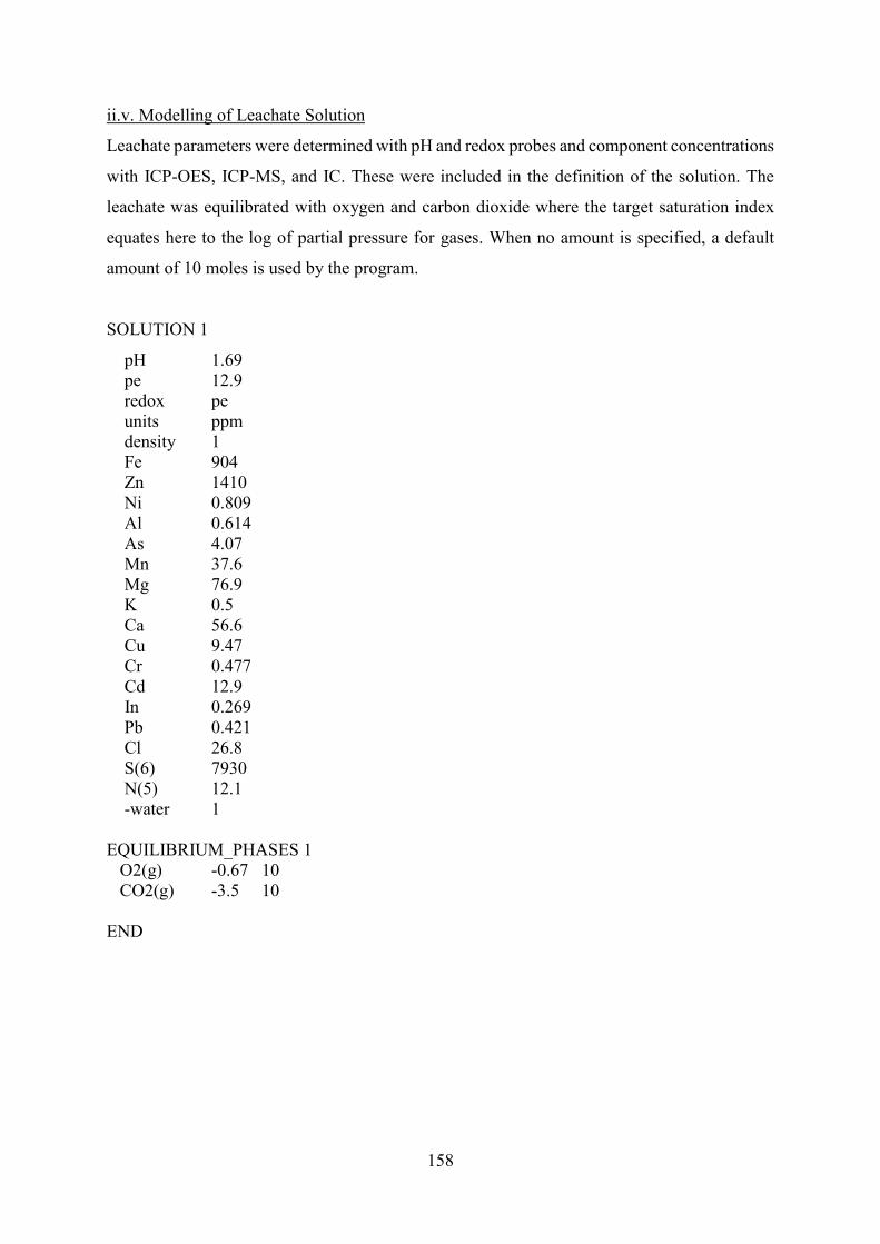
158

ii.v. Modelling of Leachate Solution

Leachate parameters were determined with pH and redox probes and component concentrations

with ICP-OES, ICP-MS, and IC. These were included in the definition of the solution. The

leachate was equilibrated with oxygen and carbon dioxide where the target saturation index

equates here to the log of partial pressure for gases. When no amount is specified, a default

amount of 10 moles is used by the program.

SOLUTION 1

pH 1.69 pe 12.9 redox pe units ppm density 1 Fe 904 Zn 1410 Ni 0.809 Al 0.614 As 4.07 Mn 37.6 Mg 76.9 K 0.5 Ca 56.6 Cu 9.47 Cr 0.477 Cd 12.9 In 0.269 Pb 0.421 Cl 26.8 S(6) 7930 N(5) 12.1 -water 1 EQUILIBRIUM_PHASES 1 O2(g) -0.67 10 CO2(g) -3.5 10 END

159

ii.vi. Abiotic Model of a Bioleaching Process

In section 8.3.2 geochemical modelling was used in an attempt to replicate the conditions of a

bioleaching experiment without the consideration of bacterial activity. The solution conditions

and mineral phases described in SOLUTION 1 and EQUILIBRIUM_PHASES 1 were

designed to be as close as possible to the experimental conditions described by BHMZ

colleagues [Gelhaar, Schopf et al. 2015]. The charge following the chloride concentration

indicates this species should be adjusted to achieve charge balance.

SOLUTION 1 temp 22 pH 2.7 pe 4 redox pe units ppm Ca 10 Cl 100 charge Fe 4020 K 1100 Mg 50 N 20 Amm 3000 P 500 S(6) 7070 -water 1 EQUILIBRIUM_PHASES 1 CO2(g) -3.5 O2(g) -0.67 Sphalerite 0 Galena 0 Pyrite 0 Quartz 0 END

160

ii.vii. Pourbaix Diagram for Iron

As with the predominance diagram, the following input file was adapted from an example

provided by Phreeplot. Here the y-axis is redox potential rather than chloride concentration.

SPECIATION jobTitle “Fe-H2O" calculationType ht1 calculationMethod 1 mainSpecies Fe xmin 0 xmax 14.0 ymin -90.0 ymax 0.0 resolution 250 PLOT plotTitle "Fe Pourbaix Diagram" xtitle pH yscale mV pymin -1000 # pymajor 500 pdf T CHEMISTRY include 'ht1.inc' SOLUTION 1 pH 0 units mmol/l Fe(3) 0.1 SAVE SOLUTION 1 END USE SOLUTION 1 EQUILIBRIUM_PHASES 1 Fix_H+ -<x_axis> NaOH 10 -force_equality true O2(g) <y_axis> Fe(OH)3(a) 0 0 END

161

ii.viii. Modelling of Electrolysis Solutions

For PHREEQC to predict indium speciation in electrowinning samples, not only did indium

stability constants have to be included in the database, but also the MGDA and MSA ligands

had to be defined as solution master species. This allowed the concentration of MGDA and

MSA to be included in the basis without defining them by their component atoms.

SOLUTION 1 units mol/L pH 2.2 In 0.523 S 0.836 MGDA 0.105

SOLUTION 2 units mol/L pH 1.5 In 0.523 Cl 0.523 MSA 2.090

162

iii. List of Tables and Figures

Table 1: List of CRMs designated by the EU commission in 2017……………………………..7

Table 2: Some typical hydro- and pyrometallurgical leaching characteristics………………..11

Table 3: Standard redox potentials of leachate metal ions, Eϴ vs Ag/AgCl 3 mol kg−1 KCl

(195 mV vs SHE) and measured E1/2 values calculated from the Ep of a DPV………...43

Table 4: Stability constants of various metal-PDCA complexes……………………………...51

Table 5: EXAFS fit parameters of 100 mmol kg−1 In3+ in 1 mol kg−1 acids with the addition of

NaCl…………………………………………………………………………………..58

Table 6: Stability constants determined with DPV and their suitability for geochemical

modelling, compared to literature values……………………………………………..82

Table 7: Equilibrium constants from this work and the literature values for the complexes of

indium with (top) nitrate, (middle) sulfate, and (bottom) chloride……………………84

Table 8: Hydrolysis constants and solubility products of indium…………………………….88

Table 9: Selected BHMZ contributing groups, aims, and collaborations during this work….105

Table 10: Concentrations of selected leachate components determined by ICP-MS and IC..111

Table 11: Results of mine water analysis……………………………………………………113

Table 12: Speciation analysis of a leachate sample predicted by PHREEQC………………..115

Table 13: Selected experimental results and predictions from a geochemical model attempting

to replicate the bioleaching experiment …………………………………………..…120

Table 14: Various filtration process defined by filter pore size……………………………...122

Table 15: Concentrations in the retentate and permeate determined by ICP-MS and IC…….123

Table 16: Hydrolysis constants and solubility products of zinc, copper, and germanium…...126

Table 17: Hydrolysis constants and solubility products of iron……………………………..127

Table 18: Ligands added to control indium speciation………………………………………129

Table 19: Diffusion coefficients determined by various electrochemical methods………….131

Table 20: Composition of indium electrowinning solutions………………………………...133

163

Figure 1: Refining of indium from the residues of zinc processing, % refers to typical weight

percentages…………………………………………………………………………….6

Figure 2: Raw materials considered by the 2017 report with highlighted CRMs………….……7

Figure 3: Map showing mineral deposits containing CRMs in Europe………………………...8

Figure 4: A schematic of the proposed BHMZ process chain with the related contributing

groups………………………………………………………………………………...10

Figure 5: The two proposed mechanisms of bacterial attack for the oxidation of sphalerite…..13

Figure 6: Thiosulfate and polysulfide leaching mechanisms of pyrite (FeS2) and sphalerite

(ZnS) respectively…………………………………………………………………….14

Figure 7: Available stability constants for (l) sulfate and (r) chloride complexes of indium…..17

Figure 8: (l) A transmission x-ray absorption spectrum µχ(E) against E where the XAS regions

are defined, (r) Fourier transform of the EXAFS region used for data analysis……….29

Figure 9: CV of a reversible redox couple Ox + e– ⇌ Red…………………………………….30

Figure 10: Deviations from the resonance frequency of a QCM crystal with deposited mass...33

Figure 11: Schematic of (l) a mercury electrode and (r) a typical 3-electrode polarographic

measurement set-up (CE = counter electrode, WE = Hg working electrode, RE =

reference electrode)…………………………………………………………………...34

Figure 12: (l) A polarographic reduction wave showing the relationship between ilim and E1/2,

(r) plot of E vs log (i/ilim–i), where n and E1/2 are calculated from the gradient and

intercept respectively…………………………………………………………………37

Figure 13: Lifetimes of faradaic, if, and non-faradaic currents, inf, after the application of a

potential pulse at t0, current measurement made at tm will contain minimum

contributions from inf…………………………………………………………………38

Figure 14: Voltage-time (l) and current-voltage plots (r) describing NPV (top) and DPV

(bottom)………………………………………………………………………………39

Figure 15: DPV measurements of 100 mg L−1 standard solutions of common leachate

components…………………………………………………………………………...42

164

Figure 16: (a) CV showing regions of no current at E1, and diffusion controlled current at E2

(b) potential-time plot and resulting (c) current-time plot for a chronoamperometry

measurement………………………………………………………………………….45

Figure 17: Structural representation of (l) a divalent metal-PCDA complex (r) post-column

PAR derivatisation agent……………………………………………………………..51

Figure 18: Simple schematic of (top) HPLC and (bottom) IC measurement set-up. With a

suitable instrument it is possible to easily switch between HPLC and IC measurements

by changing the column and the eluent………………………………………………..52

Figure 19: UV-Vis spectra of various 100 mmol kg−1 In3+ salts in 1 mol kg−1 acids. Due to the

acid concentration it is assumed that sulfuric acid is partially dissociated to HSO4–…..54

Figure 20: (l) UV-Vis spectra of indium in various ligand containing solutions, (r) changing

spectra with regard to increasing chloride concentration……………………………...55

Figure 21: Fourier transforms of the EXAFS data and fits for (l) In2(SO4)3 in H2SO4, and (r)

InCl3 in HCl…………………………………………………………………………..56

Figure 22: CVs of various 100 mmol kg−1 In3+ salts in 1 mol kg−1 acids. Due to the acid

concentration it is assumed that sulfuric acid is partially dissociated to HSO4–……….58

Figure 23: CVs of In3+/0 redox chemistry measured on various electrode surfaces……………60

Figure 24: (l) CVs on the GCE showing the changing electrochemical behaviour of indium in

the presence of various ligand anions (r) effects of ligands on reduction behaviour…..60

Figure 25: In3+ electrochemical behaviour with various concentrations of sulfate and chloride

ligands…………………………………………………………………………..…….61

Figure 26: CV and QCM data (deposited mass) plotted against time for current efficiency

determination……………………………………………………………………...….62

Figure 27: CVs of various indium samples measured on the HMDE…………………….…...63

Figure 28: Investigations regarding the reversibility of the In3+/0 couple on the HMDE……....64

Figure 29: Reduction of 1 mmol kg−1 In3+ recorded with polarography and DPV with the

hanging and dropping mercury electrode………………………………………..……66

Figure 30: DPVs (l) and plots (r) showing changing half wave reduction potentials for In3+/0

with nitrate ligand concentration, where linear fits are used to calculate x and βx……..69

165

Figure 31: DPVs (l) and plots (r) showing changing half wave reduction potentials for In3+/0

with sulfate ligand concentration, where linear fits are used to calculate x and βx……..71

Figure 32: Selected DPVs (l) and plots (r) showing the changing half wave reduction potentials

for In3+/0 with high sulfate ligand concentration, where linear fits are used to calculate

x and βx………………………………………………………………………………..73

Figure 33: DPVs (l) and plots (r) showing changing half wave reduction potentials for In3+/0

with chloride ligand concentration, where linear fits are used to calculate x and βx…...74

Figure 34: Selected DPVs (l) and plots (r) showing changing half wave reduction potentials for

In3+/0 in (top) hydroxide and (bottom) proton titrations……………………………….77

Figure 35: Re-analysis of changing half wave potential plots for (l) the hydroxide and (r) the

proton titration where presence of polynuclear indium complex In3(OH)45+ is

considered…………………………………………………………………………….78

Figure 36: Selected DPVs (l) and plots (r) showing changing half wave reduction potential for

In3+/0 plotted against pH, for a proton titration in 15 mmol kg−1 Cl–…………………...80

Figure 37: Speciation models of indium with increasing (top) nitrate, (middle) sulfate, (bottom)

and chloride concentrations using equilibrium constants from this work and values from

the literature…………………………………………………………………………..84

Figure 38: Changing half wave reduction potentials compared to modelled speciation plotted

against nitrate concentration………………………………………………………….85

Figure 39: Changing half wave reduction potentials compared to modelled speciation plotted

against sulfate concentration, where the supporting electrolyte was (l) 1 mol kg−1 KNO3

and (r) 3 mol kg−1 KNO3………………………………………………………………86

Figure 40: Changing half wave reduction potentials compared to modelled speciation plotted

against chloride concentration………………………………………………………..87

Figure 41: Geochemical model of indium hydroxide species with changing pH at (l)

0.1 mmol kg−1 In3+ and (r) 100 mmol kg−1 In3+……………………………………….88

Figure 42: Distribution of the hydrolysis products of indium, including polynuclear In3(OH)45+

and precipitation of In(OH)3 (s)………………………………………………………89

Figure 43: Distribution of the hydrolysis and chloride complexes of indium, including the

mixed species InClOH+, with respect to pH…………………………………………..90

166

Figure 44: Predominance diagram showing the formation of mixed hydroxy-halide complexes

of indium at (l) 1 mmol kg−1 and (r) 0.01 mmol kg−1 In3+……………………………...91

Figure 45: Solutions containing 1 mmol kg−1 In3+ at various pH values………………………91

Figure 46: Soluble indium concentration determined by geochemical modelling compared to

experimentally determined values using ion chromatography for solutions at various

pH values. Error bars from standard deviations in IC measurements are included but

too small to be seen…………………………………………………………………...92

Figure 47: (l) HPLC chromatogram showing retention times of benzyl-polysulfides separated

by chain length, (r) relationship between logarithmic retention time and chain

length…………………………………………………………………………………97

Figure 48: Chromatograms of polysulfide standard solutions at concentrations, (a) the detection

of short chain polysulfides at concentrations down to 10 µmol kg−1 (b) the detection of

longer chain polysulfides only possible down to ~1 mmol kg−1………………………98

Figure 49: Chromatograms of 10 mg L−1 metal standards measured in (l) oxalic acid and (r)

PDCA………………………………………………………………………………...99

Figure 50: Chromatographs showing the relationship between retention time and temperature

for a sample containing 10 mg L−1 Fe3+, In3+, Cu2+, Ni2+, and Zn2+…………………..100

Figure 51: (l) Chromatograms showing indium peak splitting with increasing concentrations of

(a) HNO3 (b) HCl, and (c) KNO3, (r) 40 mg L–1 In3+ standards diluted in various

media………………………………………………………………………………..101

Figure 52: Selected DPVs (l) and plots (r) showing changing half wave reduction potentials of

In3+/0 with PDCA concentration, where linear fits are used to calculate x and βx……102

Figure 53: Proposed in-situ bioleaching schematic, dashed arrows indicate ex-situ

electrowinning………………………………………………………………………104

Figure 54: (l) Polysulfides found in leachates compared to the 0.1 mmol kg−1 standard solution

(r) quasi-calibration curve using total polysulfide peak areas………………………..107

Figure 55: (l) Typical leachate sample and (r) variations in trace metal components of leachates

measured with DPV (dilution factor 25)…………………………………………….108

Figure 56: Standard addition of (l) zinc, cadmium, and copper using peak areas and (r) indium

and lead using peak heights to determine metal concentrations in leachates………...109

167

Figure 57: Chromatograms of the indium doped leachate resulting in an additional unidentified

peak………………………………………………………………………………….111

Figure 58: Chromatograms of the leachate diluted with PDCA with addition of indium

standards…………………………………………………………………………….111

Figure 59: Map of mine water sampling locations…………………………………………..113

Figure 60: Pourbaix diagrams showing (l) predominant sulfur species in the leachate and (r)

aqueous sulfur species when SO42– formation is supressed………………………….116

Figure 61: Dominant speciation of metal ions in the leachate between pH 0 and 7…………..118

Figure 62: Chromatograms of the retentate and permeate after membrane filtration………..123

Figure 63: Retention of indium, germanium, copper, and zinc at various pH values after

filtration of a 0.1 mmol kg−1 model solution with a nanofiltration polymer

membrane…………………………………………………………………………...124

Figure 64: Predicted speciation of 0.1 mmol kg−1 (top) zinc, (middle) copper, and (bottom)

germanium with respect to pH………………………………………………………126

Figure 65: Pourbaix diagram for aqueous iron ([Fe] = 0.1 mmol kg−1)………………………127

Figure 66: (a) Current-time plot directly after stepping to potential E2, (b) linear plot of current

density against 1/√𝑡, (r) plot showing how calculated diffusion coefficients changes

with step potential, CV shows how D remains constant after diffusion control is

reached………………………………………………………………………………130

Figure 67: DPVs to determine the diffusion coefficients of various indium species………..130

Figure 68: (l) CVs of a sample containing 100 mmol kg−1 KNO3 and (r) relationship between

peak potentials, ipc, and scan rate, √𝑣………………………………………………..131

Figure 69: Chemical structures of (l) N,N-bis(carboxymethyl)-DL-analine trisodium salt and

(r) sodium methylsulfonate………………………………………………………….134

Figure 70: DPVs (l) and plots (r) showing changing half wave reduction potentials of In3+/0

with MGDA concentration, where linear fits are used to calculate x and βx………….134

168

References

Aksel'rund and Spivakovskii. 1959. “Basic chlorides and hydroxide of indium.” Russian

Journal of Inorganic Chemistry 4 (5): 449–53

Alfantazi and Moskalyk. 2003. “Processing of indium: A review.” Minerals Engineering 16

(8): 687–94

Altynov and Ptitsyn. 1962. “Theory of the silver chloride electrode and determination of the

instability constants of complex chlorides.” Russian Journal of Inorganic Chemistry 7:

1088–91

Angerer. 2009. “Rohstoffe für Zukunfstechnologie”

Atkins and Paula. 2006. Atkins' Physical Chemistry: Oxford University Press

Aziz and Lyle. 1968. “Partition studies of chemical equilibria in indium (III) fluoride and

sulphate systems.” Journal of Inorganic and Nuclear Chemistry 30 (12): 3223–29

Baes and Mesmer. 1976. The Hydrolysis of Cations: John Wiley & Sons

Bard and Faulkner. 1980. Electrochemical Methods: John Wiley & Sons

Bard and Parsons. 1985. Standard Potentials in Aqueous Solution: Dekker

BASF. 2007. “Technical Information: Trilon® M”

BASF AG and Schneider. 1994. Use of glycine-N,N-diacetic acid derivatives as biodegradable

complexing agents for alkaline earth metal ions and heavy metal ions, and methods of

preparing them. WO9429421

Bauer, Seifert et al. 2017. “Indium-bearing sulfides from the Hämmerlein skarn deposit,

Erzgebirge, Germany: Evidence for late-stage diffusion of indium into sphalerite.”

Mineralium Deposita 27 (7): 1–18

Beck and Nagypál. 1990. Chemistry of Complex Equilibria: Wiley

Bertram. 1969. Electrochemistry at Solid Electrodes. Monographs in Electroanalytical

Chemistry and Electrochemistry: Marcel Dekker Inc.

Bertrand, Cassard et al. 2016. “Map of Critical Raw Material deposits in Europe.” Energy

Procedia 97: 44–50

Bethke. 2008. Geochemical and Biogeochemical Reaction Modeling: Cambridge University

Press

Biederman. 1956. “Studies on the hydrolysis of metal ions. Part 14: The hydrolysis of the

indium (III) ion.” Arkiv För Kemi 9: 277–93

169

Biederman, Li et al. 1961. “Studies on the hydrolysis of metal ions. Part 34: The hydrolysis of

the indium (III) ion, In3+, in 3 M (Na+) Cl– medium.” Acta Chemica Scandinavica 15:

555–64

Biederman and Wallin. 1960. “On the equilibrium In3+ + 2 In (s) ⇌ 3 In+.” Acta Chemica

Scandinavica 14: 594–608

Biryuk, Nazarenko et al. 1969. “Spectrophotometric determination of the hydrolysis constants

of indium ions.” Russian Journal of Inorganic Chemistry 14 (4): 503–6

Bjerrum. 1941. Metal Amine Formation in Aqueous Solution: Theory of the Reversible Step

Reactions: P. Haase and Son

Blasco, Gimeno et al. 2017. “Comparison of different thermodynamic databases used in a

geothermometrical modelling calculation.” Procedia Earth and Planetary Science 17:

120–23

Bond. 1980. Modern Polarographic Methods in Analytical Chemistry: M. Dekker

Bondarenko and Gorbaty. 1997. “In-situ Raman spectroscopic study of sulfur-saturated water

at 1000 bar between 200 and 500 °C.” Geochimica et Cosmochimica Acta 61 (7): 1413–

20

Bott, Feldberg et al. 1996. “Fitting experimental cyclic voltammetry data with theoretical

simulations using DigiSim 2.1.” Current Separations 15 (2): 67–71

Boulegue and Michard. 1978. “Constantes de formation des ions polysulfures S62–, S5

2– et S42–

en phase aqueuese.” Journal Francais d'Hydrologie 9: 27–33

Bozhikov, Bontchev et al. 2003. “Electrophoretic method for the determination of diffusion

coefficients of ions in aqueous solutions.” Journal of Radioanalytical and Nuclear

Chemistry 258 (3): 645–48

Brajter-Toth. 2002. Electroanalytical Methods: Guide to Experiments and Applications:

Springer-Verlag

Brauer. 1954. Handbuch der Präparativen Anorganischen Chemie: Ferdinand Enke Verlag

Brett and Brett. 1994. Electrochemistry: Principles, Methods and Applications: Oxford

Science Publications

Brown and Ellis. 1982. “The hydrolysis of metal ions. Part 4: Indium (III).” Journal of the

Chemical Society, Dalton Transactions, 1911–14

Brown and Gu. 2006. “The Chemistry of Perchlorate in the Environment.” In Perchlorate:

Environmental Occurrence, Interactions and Treatment, edited by Gu and Coates:

Springer Science+Business Media, Inc.

170

Buchert, Manhart et al. 2012. “Recycling Critical Raw Materials from waste electronic

equipment”

Busaev and Kanaev. 1959. “Computation of the stability constants of some complex

compounds of indium by the method of uniform variations using data obtained with the

aid of cationite.” Vestnik Moskovskogo Universiteta, Seriya Matematiki, Mekhaniki,

Astronomii, Fiziki, Khimii 14: 135–43

Caminiti and Paschina. 1981. “An x-ray diffraction study of the structure of the aqua indium

(III) ion in indium sulphate solution.” Chemical Physics Letters 82 (3): 487–91

Carleson and Irving. 1954. “The stability constants of the indium halides.” Journal of the

Chemical Society (Resumed), 4390–99

Chadwell, Rickard et al. 1999. “Electrochemical evidence for pentasulfide complexes with

Mn2+, Fe2+, Co2+, Ni2+, Cu2+ and Zn2+.” Aquatic Geochemistry 5 (1): 29–57

Charnock, Henderson et al. 1999. “High-temperature indium (III) solutions.” Journal of

Synchrotron Radiation 6: 607–8

Chung and Lee. 2012. “Electrochemical behaviours of indium.” Journal of Electrochemical

Science and Technology 3 (1): 1–13

Ciavatta. 1990. “The specific interaction theory in equilibrium analysis. Some empirical rules

for estimate interaction coefficients of metal ion complexes.” Annali di Chimica 80:

255–63

Ciglenečki and Ćosović. 1997. “Electrochemical determination of thiosulfate in seawater in the

presence of elemental sulfur and sulfide.” Electroanalysis 9 (10): 775–80

Colmer, Temple et al. 1950. “An iron-oxidizing bacterium from the acid drainage of some

bituminous coal mines.” Journal of Bacteriology 59: 317–28

Cook, Ciobanu et al. 2009. “Trace and minor elements in sphalerite: A LA-ICPMS study.”

Geochimica et Cosmochimica Acta 73 (16): 4761–91

Cozzi and Vivarelli. 1953. “Beitrag zur Chemie des Indiums.” Zeitschrift für Elektrochemie

57: 408–16

Crerar. 1975. “A method for computing multicomponent chemical equilibria based on

equilibrium constants.” Geochimica et Cosmochimica Acta 39 (10): 1375–84

da Silva. 2004. “Relative importance of diffusion and reaction control during the bacterial and

ferric sulphate leaching of zinc sulphide.” Hydrometallurgy 73 (3-4): 313–24

Debye and Hückel. 1923. “Zur Theorie der Elektrolyte. I. Gefrierpunktserniedrigung und

verwandte Erscheinungen.” Physikalische Zeitschrift 24: 185–2016

171

Deelstra, Vanderleen et al. 1963. “The calculation of the stability constants of some lanthanide-

α-hydroxy-carboxylate complexes using a high speed digital computer.” Bulletin des

Sociétés Chimiques Belges 72 (9-10): 632–41

Deferm, Onghena et al. 2017. “Speciation of indium (III) chloro complexes in the solvent

extraction process from chloride aqueous solutions to ionic liquids.” Dalton

Transactions 46: 4412–21

DeFord and Hume. 1951. “The determination of consecutive formation constants of complex

ions from polarographic data.” Journal of the American Chemical Society 73: 5321–22

Deichman, Rodicheva et al. 1966. “Reaction of indium sulphate with sodium sulphate in

aqueous solution.” Russian Journal of Inorganic Chemistry 11 (10): 1199–1201

Denbeigh. 1981. The Principles of Chemical Equilibrium: Cambridge University Press

Dillard, Turner et al. 1977. “Digital simulation of differential pulse polarography with

incremental time change.” Analytical Chemistry 49 (8): 1246–50

Directorate-General for Internal Market, Industry, Entrepreneurship and SMEs. 2017. “Study

of the review of the lists of Critical Raw Materials”

Dominko, Demir-Cakan et al. 2011. “Analytical detection of soluble polysulphides in a

modified Swagelok cell.” Electrochemistry Communications 13 (2): 117–20

Downs. 1993. Chemistry of Aluminium, Gallium, Indium, and Thallium: Springer

Druschel, Hamers et al. 2003. “Kinetics and mechanism of polythionate oxidation to sulfate at

low pH by O2 and Fe3+.” Geochimica et Cosmochimica Acta 67 (23): 4457–69

Emsley. 1999. The Elements: Oxford University Press

European Commission. 2011. “Report on Critical Raw Materials for the EU”

European Commission. 2014. “Report on Critical Raw Materials for the EU”

European Commission. 2017. “Report on Critical Raw Materials for the EU”

Ewing, Lilley et al. 1994. “Standard quantities in chemical thermodynamics. Fugacities,

activities and equilibrium constants for pure and mixed phases (IUPAC

Recommendations).” Pure and Applied Chemistry 66 (3): 533–52

Faisca and Victor. 1988. “Determination of trace elements in manganese metal and compounds

by ion-exchange chromatography and atomic absorption spectrometry. Part 2:

Determination of Bi, Cd, In, Zn, Pb, Fe (III); Ga, Cu (II), Co and U (VI).” Analytica

Chimica Acta 215: 317–23

Felix. 2002. Ullmann’s Encyclopedia of Industrial Chemistry: Indium and Indium Compounds:

Wiley-VCH

172

Ferguson, Dobud et al. 1968. “Coordination compounds of indium. Part 7: The stability of

indium (III) nitrate complexes in aqueous solution.” Journal of the Chemical Society A,

1058–1060

Ferri. 1972a. “On the complex formation equilibria between indium (III) and chloride ions.”

Acta Chemica Scandinavica 26: 733–46

Ferri. 1972b. “On the hydrolysis of the indium (III) ion in chloride solutions.” Acta Chemica

Scandinavica 26: 747–59

Ferri, Salvatore et al. 1994. “Complex formation equilibria at high ligand concentration:

Indium (III) chloride complexes.” Annali di Chimica 84: 141–48

Flora and Nieboer. 2002. “Determination of nickel by differential pulse polarography at a

dropping mercury electrode.” Analytical Chemistry 52 (7): 1013–20

Frenzel, Hirsch et al. 2016. “Gallium, germanium, indium, and other trace and minor elements

in sphalerite as a function of deposit type – A meta-analysis.” Ore Geology Reviews 76:

52–78

Fridman, Sorochan et al. 1962. “Stability of mixed halides of thallium and indium in solutions.”

Zhurnal Neorganicheskoi Khimii 7: 2127–33

Fthenakis, Wang et al. 2009. “Life cycle inventory analysis of the production of metals used in

photovoltaics.” Renewable and Sustainable Energy Reviews 13 (3): 493–517

Furman and Cooper. 1950. “A study of the polarographic behaviour of dropping amalgam

electrodes.” Journal of the American Chemical Society 72 (12): 5667–76

Gampp, Maeder et al. 1985. “Calculation of equilibrium constants from multiwavelength

spectroscopic data II: SPECFIT: two user-friendly programs in BASIC and standard

FORTRAN 77.” Talanta 32 (4): 257–64

Gans, Sabatini et al. 1996. “Investigation of equilbria in solution: Determination of equilibrium

constants with the HYPERQUAD suite of programs.” Talanta 43: 1739–53

Gelhaar, Schopf et al. 2015. “Indium extraction from Reiche Zeche sphalerite and community

analysis of acidic mine water.” Advanced Materials Research 1130: 392–95

George. 2004. “U.S. Geological Survey Minerals Yearbook.” USGS Survey

Gernon, Wu et al. 1999. “Environmental benefits of methanesulfonic acid.” Green Chemistry

1 (3): 127–40

Ghosh and Ray. 1991. Principles of Active Metallurgy: New Age International Ltd.

Gibson and Hayes. 2011. “Indium and Gallium Overview”

Giggenbach. 1972. “Optical spectra and equilibrium distribution of polysulfide ions in aqueous

solution at 20 °C.” Inorganic Chemistry 11 (6): 1201–7

173

Goncharuk, Bagrii et al. 2010. “The use of redox potential in water treatment processes.”

Journal of Water Chemistry and Technology 32 (1): 1–9

Graeser. 1969. “Minor elements in sphalerite and galena from Binnatal.” Contributions to

Mineralogy and Petrology 24 (2): 156–63

Grafenauer, Gorenc et al. 1969. “Physical properties and the chemical composition of

sphalerites from Yugoslavia.” Mineralium Deposita 4 (3): 275–82

Greef, Peat et al. 1985. Instrumental Methods in Electrochemistry: Woodhead Publishing Ltd.

Groot. 2001. “High-resolution x-ray emission and x-ray absorption spectroscopy.” Chemical

Reviews 101 (6): 1779–1808

Guggenheim and Turgeon. 1955. “Specific interaction of ions.” Transactions of the Faraday

Society 51: 747–61

Gupta and Mukherjee. 1990. Hydrometallurgy in Extraction Processes: CRC Press

Gurman, Binsted et al. 1986. “A rapid, exact, curved-wave theory for EXAFS calculations II:

The multiple-scattering contributions.” Journal of Physics C: Solid State Physics 19:

1845–61

Habashi. 2005. “A short history of hydrometallurgy.” Hydrometallurgy 79 (1-2): 15–22

Hakomori. 1930. “The electrode potential of indium against indium chloride solutions.”

Journal of the American Chemical Society 52: 2372–76

Han, Kondoju et al. 2002. “Recovery of indium from indium/tin oxides scrap by chemical

precipitation.” Geosystem Engineering 5 (4): 93–98

Hansen, Richter et al. 2002. “Determination of arsenic and sulfur species in environmental

samples by ion chromatography.” Analytical Chemistry 51 (6): 633–37

Hasegawa. 1970. “The behaviour of indium (III) complexes in several liquid-liquid distribution

distribution systems. I: A solvent extraction study of indium (III) complexes in aqueous

perchlorate media containing several anionic ligands.” Bulletin of the Chemical Society

of Japan 43: 2665–70

Hasegawa, Shimada et al. 1980. “Solvent extraction of 3B group metal ions from hydrochloric

acid with trioctylphosphine oxide.” Journal of Inorganic and Nuclear Chemistry 42

(10): 1487–89

Hattox and Vries. 1936. “The thermodynamics of aqueous indium sulfate solutions.” Journal

of the American Chemical Society 58: 2126–29

Hawkins and Dolan. 2014. “Understanding split peaks”

Heath and Hefter. 1977. “The use of differential pulse polarography for the determination of

stability constants.” Journal of Electroanalytical Chemistry 84: 295–302

174

Hedrick. 1999. “Rare Earths: U.S Geological Survey Minerals Yearbook.” Metals and Minerals

Heftmann. 2004. Chromatography: Fundamentals and Applications of Chromatography and

Related Differential Migration Methods: Elsevier

Henneke, Luther et al. 1997. “Sulphur speciation in anoxic hypersaline sediments from the

eastern Mediterranean Sea.” Geochimica et Cosmochimica Acta 61 (2): 307–21

Hepler and Hugus. 1952. “Hydrolysis and halide complexing of indium (III).” Journal of the

American Chemical Society 74: 6115–16

Hoffmann. 1992. “Recovering precious metals from electronic scrap.” The Journal of the

Minerals, Metals & Materials Society 44 (7): 43–48

Holleman, Wiberg et al. 2007. Lehrbuch der Anorganischen Chemie: Walter de Gruyter

Holman, Thompson et al. 2002. “Quantitative determination of sulfur-oxygen anion

concentrations in aqueous solution: Multicomponent analysis of attenuated total

reflectance infrared spectra.” Analytical Chemistry 66 (9): 1378–84

I and Nancollas. 2002. “EQUIL. General computational method for the calculation of solution

equilibriums.” Analytical Chemistry 44 (12): 1940–50

Inoue, Philipsen et al. 2012. “Electroless copper bath stability monitoring with UV-Vis

spectroscopy, pH, and mixed potential measurements.” Journal of the Electrochemical

Society 159 (7): 437–41

IUPAC. 2014. Compendium of Chemical Terminology: Gold Book

IUPAC and Academic Software. 2003. Stability Constant Database: IUPAC

Izatt, Eatough et al. 1969. “Calorimetrically determined log K, H and S values for the

interaction of sulphate ion with several bi- and ter-valent metal ions.” Journal of the

Chemical Society A: Inorganic, Physical, Theoretical, 47–53

Janrao, Pathan et al. 2014. “An overview of potentiometric determination of stability constants

of metal complexes.” Scientific Reviews and Chemical Communications 4 (1): 11–24

Jha and Prasad. 1975. “Ionic equilibria in tri-bivalent salts and corresponding thermodynamic

functions (indium alum).” Proceedings of the Nation Academy of Sciences, India 45A:

41–45

Johan. 1988. “Indium and germanium in the structure of sphalerite: an example of coupled

substitution with copper.” Mineralogy and Petrology 39 (3-4): 211–29

Johansson, Seip et al. 1961. “The crystal structure of InOH(SO4)(H2O)2.” Acta Chemica

Scandinavica 15: 1437–53

Johnson, Anderson et al. 2000. Database V8.R6.230: Lawrence Livermore National Library

175

Kaasalainen and Stefánsson. 2011. “Chemical analysis of sulfur species in geothermal waters.”

Talanta 85 (4): 1897–1903

Kamyshny, Ekeltchik et al. 2006. “Method for the determination of inorganic polysulfide

distribution in aquatic systems.” Analytical Chemistry 78 (8): 2631–39

Kamyshny, Goifman et al. 2004. “Equilibrium distribution of polysulfide ions in aqueous

solutions at 25 °C: A new approach for the study of polysulfides' equilibria.”

Environmental Science & Technology 38 (24): 6633–44

Kariuki and Dewald. 1997. “Polarographic determination of diffusion coefficient values of In

(III) in potassium chloride and nitrate supporting electrolytes.” Talanta 44 (10): 1765–

71

Kaufmann. 2003. Characterization of Materials: Wiley & Sons

Kawase, Shirai et al. 2014. “Electrochemical reactions of lithium-sulfur batteries: an analytical

study using the organic conversion technique.” Physical Chemistry Chemical Physics

16 (20): 9344–50

Kawazu and Kakiyama. 1978. “Cation-exchange chromatography of bismuth (III), cadmium

(II), indium (III), and zinc (II) ions with hydrochloric acid in aqueous acetone solution.”

Journal of Chromatography A 151 (3): 339–45

Kelly and Matos. 2015. “Historical statistics for mineral and material commodities in the

United States”

Kim, Gilmore et al. 1999. “Electrical, optical, and structural properties of indium–tin–oxide

thin films for organic light-emitting devices.” Journal of Applied Physics 86 (11):

6451–61

Koh. 1990. “Analytical chemistry of polythionates and thiosulfate.” Analytical Sciences 6 (1):

3–14

Kolthoff and Lingane. 1939. “The fundamental principles and applications of electrolysis with

the DME and Heyrovský's polarographic method of chemical analysis.” Chemical

Reviews 24: 1–94

Kondziela and Biernat. 1975. “Determination of stability constants of indium halogenide

complexes by polarography.” Journal of Electroanalytical Chemistry and Interfacial

Electrochemistry 61 (3): 281–88

Korchevin, Turchaninova et al. 1991. “Thermal transformations of allyl 2-thienyl sulfide and

selenide.” Chemistry of Heterocyclic Compounds 27 (10): 1049–52

Lee and Oh. 2004. “Analysis of ionic equilibria and electrowinning of indium from chloride

solutions.” Scandinavian Journal of Metallurgy 33: 279–85

176

Lee and Sohn. 2003. “Comparison of indium purification between vacuum refining and

electrowinning.” Journal of Materials Science 38 (24): 4843–48

Leggett, ed. 1985. Computational Methods for the Determination of Formation Constants:

Plenum Press

Licht. 1988. “Aqueous solubilities, solubility products and standard oxidation-reduction

potentials of the metal sulphides.” Journal of the Electrochemical Society 135 (12):

2971–75

Lingane. 1939. “Thermodynamic significance of polarographic half-wave potentials of simple

metal ions at the dropping mercury electrode.” Journal of the American Chemical

Society 61: 2099–2103

Liu, Avrutin et al. 2010. “Transparent conducting oxides for electrode applications in light

emitting and absorbing devices.” Superlattices and Microstructures 48 (5): 458–84

Lokanc, Eggert et al. 2015. “The availability of indium: The present, medium term, and long

term”

Losev and Molodov. 1960. “The mechanism of anode dissolution of indium amalgam in acid

solutions.” Doklady Akademii Nauk SSSR 135 (6): 1432–35.

Lovrecek and Markovac. 1962. “Studies of the electrochemical kinetics of indium. I: Kinetics

of deposition and dissolution in the indium + indium sulphate system.” Journal of the

Electrochemical Society 109 (8): 727–31

Luther. 1991. “Pyrite synthesis via polysulfide compounds.” Geochimica et Cosmochimica

Acta 55: 2839–49

Luther, Giblin et al. 1985. “Polarographic analysis of sulfur species in marine porewaters.”

Limnology and Oceanography 30 (4): 727–36

Mahaseth, Jha et al. 1994. “Ionic equilibria in tri-bivalent salts (indium alum) at 15 ºC.” Asian

Journal of Chemistry 6 (3): 619–25

Mahaseth, Jha et al. 1995a. “A recalculation of the dissociation constants of InSO4+ and the

corresponding thermodynamic functions.” Asian Journal of Chemistry 7 (2): 405–12

Mahaseth, Jha et al. 1995b. “A recalculation of the first dissociation constant of In(SO4)2– and

the corresponding thermodynamic functions.” Asian Journal of Chemistry 7 (1): 55–61

Marinoni, Carrayrou et al. 2017. “Thermodynamic equilibrium solutions through a modified

Newton Raphson method.” AIChE Journal 63 (4): 1246–62

Markovac and Lovrecek. 1965. “Studies of the electrochemical kinetics of indium. II: System

indium + indium sulphate at higher CD.” Journal of the Electrochemical Society 112

(5): 520–24

177

Martell and Motekaitis. 1990. “Potentiometry revisited: The determination of thermodynamic

equilibria in complex multicomponent systems.” Coordination Chemistry Reviews 100:

323–61

Martell and Motekaitis. 1992. Determination and Use of Stability Constants: VCH

Massalski. 2007. Binary Alloy Phase Diagrams: ASM International

Matsuda and Ayabe. 1955. “Zur Theorie der Randles‐ Sevčikschen Kathodenstrahl‐

Polarographie.” Zeitschrift für Elektrochemie 59 (6): 494–503

Melin and Rautenbach. 2003. Membranverfahren: Grundlagen der Modul- und

Anlagenauslegung: Springer

Miceli and Stuehr. 1968. “Ligand penetration rates into metal ion coordination spheres,

aluminium (III), gallium (III), and indium (III) sulfates.” Journal of the American

Chemical Society 90 (25): 6967–72

Mikhailova, Nacheva et al. 1969. “Stability constants of chloride complexes of indium in the

presence of alkali metal nitrates as the supporting electrolyte.” Radiokhimiya 11: 241–

45

Mikolajczak. 2010. “Verfügbarkeit von Indium und Gallium.” Galvanotechnik 2: 390–92

Milićev and Stergaršek. 1989. “Qualitative and quantitative determination by Raman

spectroscopy of different sulphur oxoacid anions, existing in equilibrium in oxidized

leach liquors, produced by desulphurization of flue gases.” Spectrochimica Acta Part

A: Molecular Spectroscopy 45 (2): 225–28

Misra and Dubinskii. 2002. Ultraviolet Spectroscopy and UV Lasers: Marcel Dekker

Moeller. 1941. “Contributions to the chemistry of indium. II: The hydrolysis of indium

trichloride solutions.” Journal of the American Chemical Society 63: 1206–7

Moeller. 1942. “Contributions to the chemistry of indium. V: Hydrolysis constants for indium

tribromide and triiodide solutions.” Journal of the American Chemical Society 64: 953–

54

Moses. 1984. “Sampling and analysing mixtures of sulphate, sulphite, thiosulphate and

polythionate.” Talanta 31 (5): 331–39

Moss, Tzimas et al. 2011. “Critical metals in strategic energy technologies: Assessing rare

metals as supply-chain bottlenecks in low-carbon energy technologies”

Nanda and Aditya. 1962. “Studies on ion association equilibria, spectrophotometric

dertermination of the thermodynamic instability constants of AlSO4+, GaSO4

+ and

InSO4+.” Zeitschrift für Physikalische Chemie 35: 139–45

178

Narita, Tanaka et al. 2014. “Structural properties of the inner coordination sphere of indium

chloride complexes in organic and aqueous solutions.” Dalton Transactions 43 (4):

1630–35

O’Reilly, Dicinoski et al. 2001. “Chromatographic and electrophoretic separation of inorganic

sulfur and sulfur–oxygen species.” Analytica Chimica Acta 432 (2): 165–92

Okamoto and Takebayashi. 1995. Method for recovering indium by electrowinning. 5543031A

Oldham and Parry. 1970. “Characterisation of electrode reversibility by pulse polarography.”

Analytical Chemistry 42 (2): 229–33

Pang, Liang et al. 2015. “Review - The importance of chemical interactions between sulfur

host materials and lithium polysulfides for advanced lithium-sulfur batteries.” Journal

of the Electrochemical Society 162 (14): 2567–76

Paoletti, Vacca et al. 1966. “Computer calculation of stepwise stability constants and heat

changes from calorimetric data. System silver (I)-pyridine.” The Journal of Physical

Chemistry 70 (1): 193–96

Parker and Prisk. 1953. “The oxidation of inorganic compounds of sulfur by various sulfur

bacteria.” Journal of General Microbiology 8: 344–64

Parkhurst and Appelo. 2013. Description of input and examples for PHREEQC version 3 – A

computer program for speciation, batch-reaction, one-dimensional transport, and

inverse geochemical calculations. U.S. Geological Survey Techniques and Methods

Parriott. 2012. A Practical Guide to HPLC Detection: Academic Press

Parry and Osteryoung. 1965. “Evaluation of analytical pulse polarography.” Analytical

Chemistry 37 (13): 1634–37

Petrosyants and Ilyukhin. 2011. “Indium (III) coordination compounds.” Russian Journal of

Inorganic Chemistry 56 (13): 2047–69

Petrow and Strehlow. 1967. “Spectrophotometric determination of thorium in bone ash using

Arsenazo III.” Analytical Chemistry 39 (2): 265–67

Piercy and Hampson. 1975. “The electrochemistry of indium.” Journal of Applied

Electrochemistry 5: 1–15

Pihlar, Valenta et al. 1981. “New high-performance analytical procedure for the voltammetric

determination of nickel in routine analysis of waters, biological materials and food.”

Fresenius' Zeitschrift für Analytische Chemie 307 (5): 337–46

Pitzer. 1991. Activity Coefficients in Electrolyte Solutions: CRC Press

Pokorna and Zabranska. 2015. “Sulfur-oxidizing bacteria in environmental technology.”

Biotechnology Advances 33: 1246–59

179

Pokrovski and Dubrovinsky. 2011. “The S3– ion is stable in geological fluids at elevated

temperatures and pressures.” Science 331 (6020): 1052–54

Potvin. 1990. “Modelling complex solution equilibria. I: Fast, worry-free least-squares

refinement of equilibrium constants.” Canadian Journal of Chemistry 68 (12): 2198–

2207

Powalla and Dimmler. 2000. “Scaling up issues of CIGS solar cells.” Thin Solid Films 361:

540–46

Ravel and Newville. 2005. “Athena, Artemis, Hephaestus: Data analysis for x-ray absorption

spectroscopy using IFEFFIT.” Journal of Synchrotron Radiation 12 (4): 537–41

Rawlings and Johnson. 2007. Biomining: Springer

Rehr and Albers. 2000. “Theoretical approaches to x-ray absorption fine structure.” Reviews of

Modern Physics 72 (3): 621–54

Reich and Richter. 1863. “Über das Indium.” Journal für Praktische Chemie 90: 172–76

Ricciu, Secco et al. 2000. “Kinetics and equilibria of the interaction of indium (III) with

pyrocathecol violet by relaxation spectrometry.” The Journal of Physical Chemistry A

104 (30): 7036–43

Rizkov, Lev et al. 2004. “Development of in-house reference materials for determination of

inorganic polysulfides in water.” Accreditation and Quality Assurance 9 (7): 399–403

Roex and Watkins. 1990. “Analysis of rare-earth elements in geological samples by gradient

ion chromatography: An alternative to ICP and INAA.” Chemical Geology 88 (1-2):

151–62

Rossotti and Rossotti. 1956. “Studies on the hydrolysis of metal ions. Part 15: Partition

equilibria in the system 114In/TTA/benzene.” Acta Chemica Scandinavica 10: 779–92

Rossotti and Rossotti. 1961. The Determination of Stability Constants and Other Equilibrium

Constants in Solution: McGraw-Hill Book Company Inc.

Rozan, Theberge et al. 2000. “Quantifying elemental sulfur (S0), bisulfide (HS−) and

polysulfides (Sx2−) using a voltammetric method.” Analytica Chimica Acta 415 (1-2):

175–84

Rudolph, Fischer et al. 2004. “Indium (III) hydration in aqueous solutions of perchlorate,

nitrate and sulfate. Raman and infrared spectroscopic studies and ab-initio molecular

orbital calculations of indium (III)-water clusters.” Physical Chemistry Chemical

Physics 6 (22): 5145–55

Sand, Gehrke et al. 2001. “(Bio)chemistry of bacterial leaching – direct vs. indirect

bioleaching.” Hydrometallurgy 59 (2-3): 159–75

180

Sand, Schippers et al. 1995. “Sulfur chemistry, biofilm, and the (in)direct attack mechanism -

a critical evaluation of bacterial leaching.” Applied Microbiology and Biotechnology

43: 961–66

Schippers. 2004. “Biogeochemistry of metal sulfide oxidation in mining environments,

sediments, and soils.” In Sulfur Biogeochemistry: Past and Present, edited by Amend

et al. Geological Society of America

Schippers. 2009. “Biomining for metal extraction from ore and waste.” Advanced Mineralogy

Solutions 1: 27–33

Schippers, Rohwerder et al. 1999. “Intermediary sulfur compounds in pyrite oxidation -

implications for bioleaching and biodepyritization of coal.” Applied Microbiology and

Biotechnology 52: 104–10

Schippers, Sand et al. 1996. “Sulphur chemistry in the bacterial leaching of pyrite.” Applied

Environmental Microbiology 62 (9): 3424–31

Schippers and Sand. 1999. “Bacterial leaching of metal sulphides proceeds by two indirect

mechanisms via thiosulphate or via polysulphides and sulphur.” Applied Environmental

Microbiology 65 (1): 319–21

Schischkova. 1978. “Komplexbildung von Indium (III) in wässrigen und wässrigorganischen

Lösungen verschiedener Sulfate.” Comptes rendus de l'Académie bulgare des Sciences

31 (8): 995–98

Schufle and Eiland. 1954. “Indium halide complexes studied by ion-exchange methods.”

Journal of the American Chemical Society 76: 960–62

Schufle, Stubbs et al. 1951. “A study of indium (III) chloride complexes by polarographic

methods.” Journal of the American Chemical Society 73: 1013–15

Schwarzenbach and Fischer. 1960. “Die Acidität der Sulfane und die Zusammensetzung

wässeriger Polysulfidlösungen.” Helvetica Chimica Acta 43 (5): 1365–90

Schwarzenbach, Flaschka et al. 1969. Complexometric Titrations: Methuen

Schwarz-Schampera and Herzig. 2002. Indium: Geology, Mineralogy and Economics:

Springer

Seward, Henderson et al. 2000. “Indium (III) chloride complexing and solvation in

hydrothermal solutions to 350 °C: an EXAFS study.” Chemical Geology 167 (1-2):

117–27

Silverman and Ehrlich. 1964. “Microbial Formation and Degradation of Minerals.” In

Advances in Applied Microbiology, edited by Umbreit: Academic Press

181

Silverman and Lundgren. 1959. “Studies on the chemoautotrophic iron bacterium

Ferrobacillus ferrooxidans. I: An improved medium and a harvesting procedure for

securing high cell yields.” Journal of Bacteriology 77 (5): 642–47

Sinclair and Worral. 1982. “Neutral complexes of the indium dihalides.” Canadian Journal of

Chemistry 60: 695–98

Skoog, Holler et al. 2008. Principles of Instrumental Analysis: Saunders College Publications

Spencer. 1973. “Spectrophotometric determination of an equilibrium constant.” Journal of

Chemical Education 50 (4): 298–99

Stackelberg and Freyhold. 1940. “Polarographische Untersuchungen an Komplexen in

wässriger Lösung.” Zeitschrift für Elektrochemie 46 (3): 120–29

Starkey. 1935. “Products of the oxidation of thiosulfate by bacteria in mineral media.” The

Journal of General Physiology 18 (3): 325–49

Stefánsson. 2007. “Iron (III) hydrolysis and solubility at 25 °C.” Environmental Science &

Technology 41 (17): 6117–23

Stern. 2001. “Musings about the development of XAFS.” Journal of Synchrotron Radiation 8:

49–54

Steudel, Holdt et al. 1989. “Ion-pair chromatographic separation of inorganic sulphur anions

including polysulphides.” Journal of Chromatography 475: 442–46

Strelow. 1988. “Determination of indium in a matrix of cadmium, mercury and tellurium by

ion exchange chromatography and graphite furnace atomic absorption spectroscopy.”

Journal of Analytical Atomic Spectrometry 3: 183–86

Sundén. 1953. “On the complex chemistry of the indium ion. Part I: The acetate, formiate,

propionate and glycolate systems.” Svensk Kemisk Tidskrift 65 (12): 257–74

Sundén. 1954a. “On the complex chemistry of the indium ion. Part II: The chloride, bromide

and sulphate systems.” Svensk Kemisk Tidskrift 66 (1): 20–33

Sundén. 1954b. “On the complex chemistry of the indium ion. Part IV: An investigation of the

chloride and sulphate systems by ion exchangers.” Svensk Kemisk Tidskrift 66 (5-6):

173–78

Sundén. 1954c. “On the complex chemistry of the indium ion. Part V: The chloride, bromide

and sulphate systems from extraction equilibria.” Svensk Kemisk Tidskrift 66 (12): 345–

50

Szekeres. 1974. “Analytical chemistry of the sulphur acids.” Talanta 21 (1): 1–44

Teder. 1971. “The equilibrium between elementary sulfur and aqueous polysulfide solutions.”

Acta Chemica Scandinavica 25: 1722–28

182

Tolcin. 2017. “Indium: USGS Mineral Commodity Summaries.” USGS Survey

Torrance and Gatford. 1985. “Differential pulse stripping voltammetry for the determination

of nickel and cobalt in simulated PWR coolant.” Talanta 32 (4): 273–78

Tributsch. 2001. “Direct versus indirect bioleaching.” Hydrometallurgy 59 (2-3): 177–85

Tuck. 1983. “Critical evaluation of equilibrium constants in solution. Part A: Stability constants

of metal complexes: Critical survey of stability constants of complexes of indium.”

Pure and Applied Chemistry 55 (9): 1477–1528

Tunaboylu and Schwarzenbach. 1970. “Die Löslichkeit von Indiumsulfid.” Chimia 24: 424–

27

Turner, Whitfield at al. 1981. “The equilibrium speciation of dissolved components in

freshwater and seawater at 25 ºC and 1 atm pressure.” Geochimica et Cosmochimica

Acta 45: 855–81

Turnham. 1965. “The polarographic diffusion coefficients of some simple cations in various

electrolytes, calculated for infinite dilution and under polarographic conditions.”

Journal of Electroanalytical Chemistry 10: 19–27

Tur'yan and Strizhov. 1972. “Polarographic determination of the instability constant of the

sulphato-complex of indium (III).” Russian Journal of Inorganic Chemistry 17 (7):

1066–67

Tur’yan, Tikhanov et al. 1982. “Electroreduction of In (III) ions catalysed by halide and

thiocyanate ions, and the polarographic determination of the stability constants of

halide and thiocyanate complexes if indium” Russian Journal of General Chemistry 52:

1520–25

USGS. 1962. “Chemistry of iron in natural water.” U.S. Geological Survey

Umiker, Morra et al. 2002. “Aqueous sulfur species determination using differential pulse

polarography.” Microchemical Journal 73 (3): 287–97

Vavra and Rudenko. 1964. “Sorption of indium on Kationite KU-2 and stability constants of

indium chloride complexes in water-ethanol solutions.” Vestnik Moskovskogo

Universiteta, Khimiya 6: 14–17

Vera, Schippers et al. 2013. “Progress in bioleaching: Fundamentals and mechanisms of

bacterial metal sulfide oxidation – Part A.” Applied Microbiology and Biotechnology

97 (17): 7529–41

Vijayakumar, Govind et al. 2014. “Molecular structure and stability of dissolved lithium

polysulfide species.” Physical Chemistry Chemical Physics 16 (22): 10923–32

183

Visco. 1965. “Kinetics and equilibrium of the system indium (III) - indium (I) - indium (0) in

acidic solutions.” Journal of Physical Chemistry 69: 202–7

Vitha. 2016. Chromatography: Principles and Instrumentation: John Wiley & Sons

Vostal, Šingliar et al. 2017. “Method for the recovery of indium from diluted bioleaching

solutions.” Solid State Phenomena 262: 265–68

Weiß. 2001. Ionenchromatographie: Wiley-VCH

Wen-Ju, Jui-Ju et al. 2003. “Standard Gibbs energies of transfer of In (III) ion.” Acta Physica

Sinica 19 (3): 230–32

White and Hemond. 2012. “The anthrobiogeochemical cycle of indium: A review of the natural

and anthropogenic cycling of indium in the environment.” Critical Reviews in

Environmental Science and Technology 42 (2): 155–86

White, Kelly et al. 1961. “Dinonyl naphthalene sulphonic acid and tri-n-octylamine as liquid

ion-exchangers for the study of Fe (III) and In (III) chloride complexes.” Journal of

Inorganic and Nuclear Chemistry 16: 337–44

Wincott and Vaughan. 2006. “Spectroscopic studies of sulfides.” Reviews in Mineralogy and

Geochemistry 61 (1): 181–229

Woollacott and Eric. 1994. Mineral and Metal Extraction: An Overview: South African

Institute of Mining and Metallurgy

Yan, Zhang et al. 1988. “Ionen-Chromatographie von Gallium, Indium und Thallium mit

Anwendungen in der Erzanalyse.” Fresenius' Zeitschrift für Analytische Chemie 331

(6): 601–6

Zekany and Nagypal. 1985. “PSEQUAD.” In Computational Methods for the Determination

of Formation Constants, edited by Leggett: Plenum Press

Zelyanskaya, Bausova et al. 1958. “Polarographic properties of gallium and indium.” Trudy

Institut Metallurgi, Academia Nauk SSR, Ural Filial 2: 263–74

Zhu and Anderson. 2002. Environmental Applications of Geochemical Modeling: Cambridge

University Press