Electrochemical Modeling of a single Li{Ion cell€¦ · Institute of Electrical Measurement and...

Institute of Electrical Measurement and Measurement Signal Processing

Electrochemical Modeling

of a single Li–Ion cell

Martin Sommer

Konstanz, Marz 4, 2010

Martin Sommer Konstanz, Marz 4, 2010 Electrochemical Modeling

1 / 31


Overview

� Modeling approaches

� Equivalent circuit model

� Electrochemical model

� Mathematical Model of the electrochemical system

� Numerical realization

� Method

� Discretization in space

� Discretization in time

� Simulation Results

� Problems


2 / 31


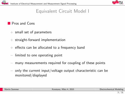
Equivalent Circuit Model I

� Pros and Cons

+ small set of parameters

+ straight-forward implementation

+ effects can be allocated to a frequency band

− limited to one operating point

− many measurements required for coupling of these points

− only the current input/voltage output characteristic can bemonitored/displayed


3 / 31


Equivalent Circuit Model II

Abbildung 1: Simple RC–model with additional impedance ZW for lowfrequencies.

Abbildung 2: Nyquist plot of a Li–Ion battery showing a characteristic halfcircle and a 45◦ straight line.


4 / 31


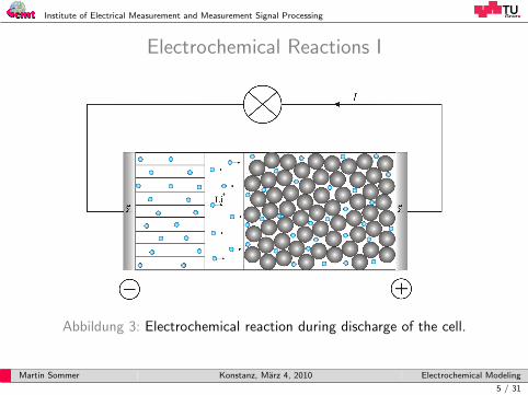
Electrochemical Reactions I

Abbildung 3: Electrochemical reaction during discharge of the cell.


5 / 31


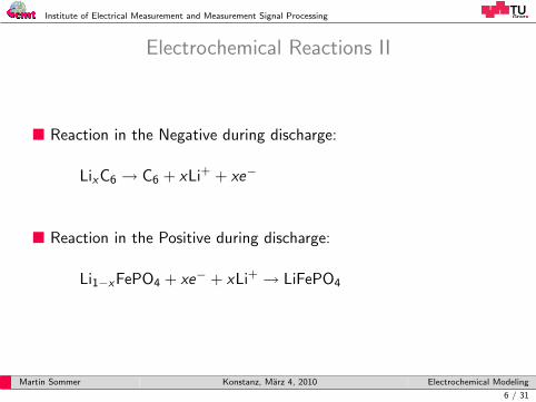
Electrochemical Reactions II

� Reaction in the Negative during discharge:

LixC6 → C6 + xLi+ + xe−

� Reaction in the Positive during discharge:

Li1−xFePO4 + xe− + xLi+ → LiFePO4


6 / 31


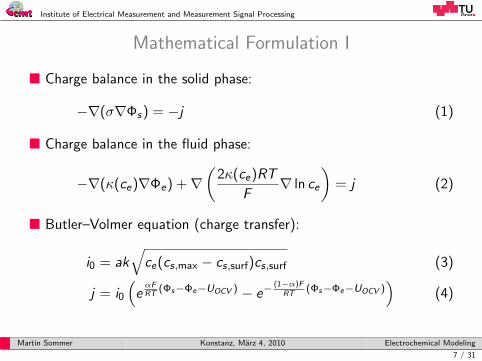
Mathematical Formulation I

� Charge balance in the solid phase:

−∇(σ∇Φs) = −j (1)

� Charge balance in the fluid phase:

−∇(κ(ce)∇Φe) +∇(

2κ(ce)RT

F∇ ln ce

)= j (2)

� Butler–Volmer equation (charge transfer):

i0 = ak√

ce(cs,max − cs,surf)cs,surf (3)

j = i0(

eαFRT

(Φs−Φe−UOCV ) − e−(1−α)F

RT(Φs−Φe−UOCV )

)(4)


7 / 31


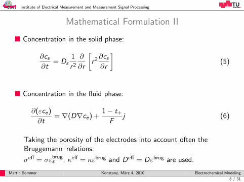
Mathematical Formulation II

� Concentration in the solid phase:

∂cs

∂t= Ds

1

r 2

∂

∂r

[r 2∂cs

∂r

](5)

� Concentration in the fluid phase:

∂(εce)

∂t= ∇(D∇ce) +

1− t+

Fj (6)

Taking the porosity of the electrodes into account often theBruggemann–relations:

σeff = σεbrugs , κeff = κεbrug and Deff = Dεbrug are used.


8 / 31


Boundary Conditions

� Charge balance in the solid phase:

−σ∇Φs = i fur x = 0, x = L

� Charge balance in the fluid phase:

−(κ(ce)∇Φe) +(

2κ(ce)RTF ∇ ln ce

)= 0 fur x = 0, x = L


−Ds∂cs∂r |r=0 = 0, −Ds

∂cs∂r

∣∣∣r=Rs = jaF


∇ce = 0 fur x = 0, x = L

Additionally a reference potential has to be defined! (e.g. Φs(0) = 0)


9 / 31


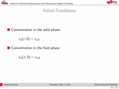
Initial Conditions


cs(r , 0) = cs,0


ce(x , 0) = ce,0


10 / 31


Modifications of the Equation System I

� Modification of the fluid potential after [1]:

Φe = Φe − 2κ(ce)RTF ln ce

therby the charge balance in the fluid results as follows

−∇(κ(ce)∇Φe) = j (7)

as well as

j = i0(

eαFRT

(Φs−(Φe+ 2κ(ce )RTF

ln ce)−UOCV)

−e−(1−α)F

RT(Φs−(Φe+ 2κ(ce )RT

Fln ce)−UOCV )

) (8)

for the Butler–Volmer equation.


11 / 31


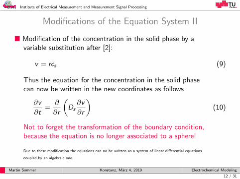
Modifications of the Equation System II

� Modification of the concentration in the solid phase by avariable substitution after [2]:

v = rcs (9)

Thus the equation for the concentration in the solid phasecan now be written in the new coordinates as follows

∂v

∂t=

∂

∂r

(Ds∂v

∂r

)(10)

Not to forget the transformation of the boundary condition,because the equation is no longer associated to a sphere!

Due to these modification the equations can no be written as a system of linear differential equations

coupled by an algebraic one.


12 / 31


The Control Volume Method I

� CVM on the example of the charge transfer in the solid phase [3]:

−∇(σ∇Φs) = −j (11)

The integration of the equation for the 1D case yields

−(σ

dΦs

dx

)e

−(−σdΦs

dx

)w

= −e∫

w

j dx . (12)

This equation can be discretized as follows

−(σe(Φs,E − Φs,P)

(δx)e

)+

(σw (Φs,P − Φs,W )

(δx)w

)= −j ∆x . (13)


13 / 31


The Control Volume Method II

This brings us to a linear equation for each discretization point

aPΦs,P = aE Φs,E + aW Φs,W + b (14)

with the coefficients

aE = σe(δx)w

, aW = σw(δx)w

, aP = aE + aW and b = j ∆x .

The resulting set of equations is symmetric showing a tridiagonalstructure. Systems of that kind can be solved by simple algorithms.


14 / 31


The Control Volume Method III

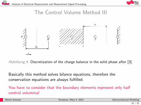
Abbildung 4: Discretization of the charge balance in the solid phase after [3].

Basically this method solves bilance equations, therefore theconservation equations are always fulfilled.

You have to consider that the boundary elements represent only halfcontrol volumina!


15 / 31


The Control Volume Method IV

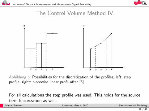
Abbildung 5: Possibilities for the discretization of the profiles; left: stepprofile, right: piecewise linear profil after [3].

For all calculations the step profile was used. This holds for the sourceterm linearization as well.


16 / 31


The Control Volume Method V

� Time discretization on the example of the modified concentrationequation in the solid phase (fully implicit scheme):

∂v

∂t=

∂

∂r

(Ds∂v

∂r

)(15)

(v 1P − v 0

P)

∆t∆r =

(Ds,e(v 1

E − v 1P)

(δr)e

)−(

Ds,w (v 1P − v 1

W )

(δr)w

)(16)

with the new coefficients for the equation system

aE =Ds,e

(δr)w, aW =

Ds,w

(δr)e, a0

P = ∆r∆t , aP = aE + aW + a0

P

and b = a0Pv 0

P .

This discretization has the advantage that its always stable!


17 / 31


The Finite Difference Method

� Discretization on the example of the concentration in the solidphase after [4]:

∂cs

∂t= Ds

1

r 2

∂

∂r

[r 2∂cs

∂r

](17)

∂cs,P

∂t=

Ds,e

∆r(δr)e

r 2e

r 2p

(cs,E − cs,P)− Ds,w

∆r(δr)w

r 2w

r 2p

(cs,P − cs,W ) (18)

This discretization leads to an asymmtric system matrix!


18 / 31


Implementation in Matlab R© I

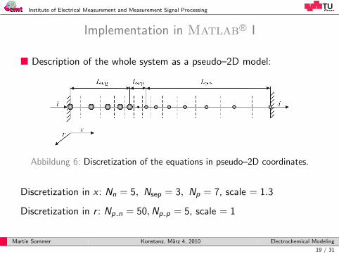
� Description of the whole system as a pseudo–2D model:

Abbildung 6: Discretization of the equations in pseudo–2D coordinates.

Discretization in x : Nn = 5, Nsep = 3, Np = 7, scale = 1.3

Discretization in r : Np n = 50,Np p = 5, scale = 1


19 / 31


Implementation in Matlab R© II

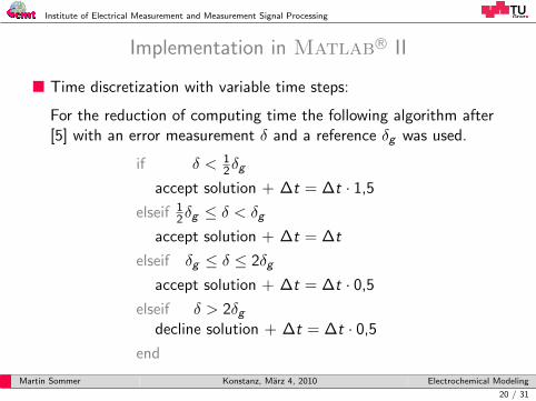
� Time discretization with variable time steps:

For the reduction of computing time the following algorithm after[5] with an error measurement δ and a reference δg was used.

if δ < 12δg

accept solution + ∆t = ∆t · 1,5

elseif 12δg ≤ δ < δg

accept solution + ∆t = ∆t

elseif δg ≤ δ ≤ 2δg

accept solution + ∆t = ∆t · 0,5

elseif δ > 2δgdecline solution + ∆t = ∆t · 0,5

end


20 / 31


Implementation in Matlab R© III

The error measurement is determined as follows

δ =‖vf − vc‖2

‖vf ‖2

, (19)

with vf being calculated using ∆t2 and vc using ∆t for the step size.

For the diffusion equations in the solid phased

δg = 1e−2 was used.

For the concentration in the liquid phase

δg = 1e−3 was used.

The step size can vary in the interval1 ms < ∆t < 60 s .


21 / 31


Implementation in Matlab R© IV

Abbildung 7: Error due to nonlinearity in t after [6].

Strong nonlinearities can lead to errors using a coarse step size!


22 / 31


Implementation in Matlab R© V

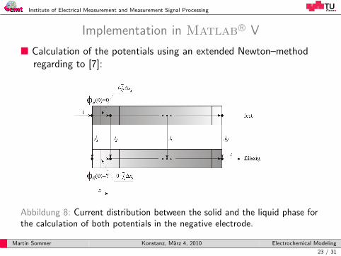
� Calculation of the potentials using an extended Newton–methodregarding to [7]:

Abbildung 8: Current distribution between the solid and the liquid phase forthe calculation of both potentials in the negative electrode.


23 / 31


Implementation in Matlab R© VI

For the negtive electrode the potential φe(0) is varied until the cur-rent is transferred from to solid to the liquid phase or vice versa.

i =

∫jdx =

∑k

jk∆xk (20)

For the positive electrode the reaction runs into the opposite direc-tion. The only difference is now that φe(Ln + Lsep) is known andφs(Ln + Lsep) has to be determined.

stopping criteria:

(i −∑k

jk∆xk) ≤ 1e−6, maxiter= 500, smin = 1 pV, smax p = 50 mV,

smax n = 100 mV .


24 / 31


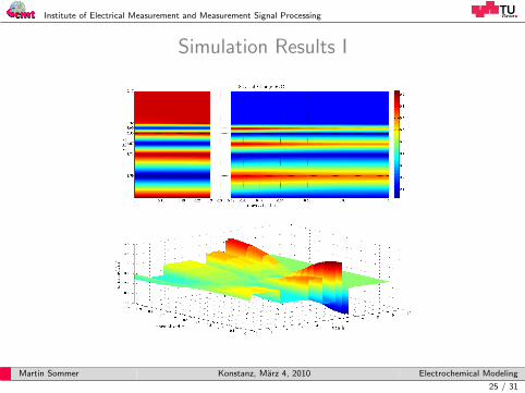
Simulation Results I


25 / 31


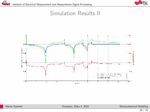
Simulation Results II


26 / 31


Problems

� Dealing with source term in potential equations (iterativemethods)

� Discretization dependencies (not known)

� Low i0 causes problems

� Number of parameters

� Errors

� Physics

� Mathematical Formulation

� Realization


27 / 31


Thank You For Your Attention!


28 / 31


Literatur I

J. Wu, J.Xu, H. Zou: On The Well Posedness Of A MathematicalModel For Lithium–Ion Battery Systems, Methods andApplications of Analysis, vol. 13, no. 3, 2006, S. 275–298

A. J. Bard, L.R. Faulkner: Electrochemical Methods:Fundamentals and Applications, John Wiley & Sons, 2nd edition,2001, S. 165

S. V. Patankar: Numerical Heat Transfer and Fluid Flow, series incomputational methods in mechanics and thermal sciences, 1980

L. Cai, R. E. White: Reduction of Model Order Based on ProperOrthogonal Decomposition for Lithium–Ion Battery Simulations,Journal of The Electrochemical Society, vol. 156, no. 3, 2009,S. 154–161


29 / 31


Literatur II

S. E. Minkoff, N. M. Kridler: A comparison of adaptive timestepping methods for coupled flow and deformatio modeling,Applied Mathematical Modeling, vol. 30, no. 9, 2006, S. 993-1009

E. Kreyszig: Advanced Egeneering Mathematics, John Wiley &Sons, 7th edition, 1993, S. 1035 ff.

B. Schweighofer: Simulation of the Dynamic Behavior of aLead–Acid Battery, Dissertation an der TUGraz, 2007


30 / 31

The author wishes to thank the “COMET K2 Forschungsförderungs-Programm” of the Austrian Federal Ministry for Transport, Innovation and Technology (BMVIT), the Austrian Federal Ministry of Economics and Labour (BMWA), Österreichische Forschungsförderungsgesellschaft mbH (FFG), Das Land Steiermark, and Steirische Wirtschaftsförderung (SFG) for their financial support.Additionally, we would like to thank the supporting companies and project partners

as well as

Electrochemical Modeling of a single Li{Ion cell€¦ · Institute of Electrical Measurement and...

Documents

Transcript of Electrochemical Modeling of a single Li{Ion cell€¦ · Institute of Electrical Measurement and...