Electricity markets - CERMICSdelmas/Enseig/levy-delatour-market.pdf · Electricity markets February...
73
Electricity markets February 2016 Arnaud de Latour, [email protected] Outline ELECTRICITY MARKET DESIGN The electricity value chain Electricty market microstructure (balancing mechanism) Tools for power generation, typical supply curve in electricity markets Key drivers of European electricity prices MODELLING ELETRICITY PRICES Main features of power prices Overview of spot and forward models A structural model for electricity prices (Aïd et al., 2011) Factorial models for energy prices (e.g. Kiesel et al., 2008) Disclaimer ! Any views or opinions presented in this presentation are solely those of the author and do not necessarily represent those of the EDF group. 1 – Electricity markets
Transcript of Electricity markets - CERMICSdelmas/Enseig/levy-delatour-market.pdf · Electricity markets February...
Electricity markets
February 2016 Arnaud de Latour, [email protected]
Outline
ELECTRICITY MARKET DESIGN
The electricity value chain
Electricty market microstructure (balancing mechanism)
Tools for power generation, typical supply curve in electricity markets
Key drivers of European electricity prices
MODELLING ELETRICITY PRICES
Main features of power prices
Overview of spot and forward models
A structural model for electricity prices (Aïd et al., 2011)
Factorial models for energy prices (e.g. Kiesel et al., 2008)
Disclaimer ! Any views or opinions presented in this presentation are solely those of the author and do not necessarily represent those of the EDF group.
1 – Electricity markets
ELECTRICITY MARKET DESIGN
2 – Electricity markets
Some generalities, the electricity value chain
Electricity market microstructure
Power production tools and drivers of European electricity prices
Main electricity features Electricity is a local commodity due to the non-storability and transport constraints
Electricity is a local commodity :
Electricity is non-storable
Present best way to store large volumes of power: hydro-reservoir.
A too long excess of demand compared to supply may lead to dramatic blackouts (example in July 30th, 2012: India, 670 millions people).
⇨ Minute by minute real-time assessment of the equilibrium between demand and supply
Electricity transport satisfies specific laws (Kirchhoff's laws).
In a meshed electricity network, power will go from one point to another using all available paths, causing possible electricity flow interference.
⇨ Cross-border trading opportunities, up to transfert capacities available
A common market structure for a local commodity :
Electricity being a local commodity, there are as many electricity markets as they are states…
Market microstructure highly depends on national regulation.
Nevertheless, common structure emerges driven by the necessary equilibrium between consumption and production.
A central role of the Transport System Operator, in France : RTE and in Europe : ENTSO (European Network System Operator).
3 – Electricity markets
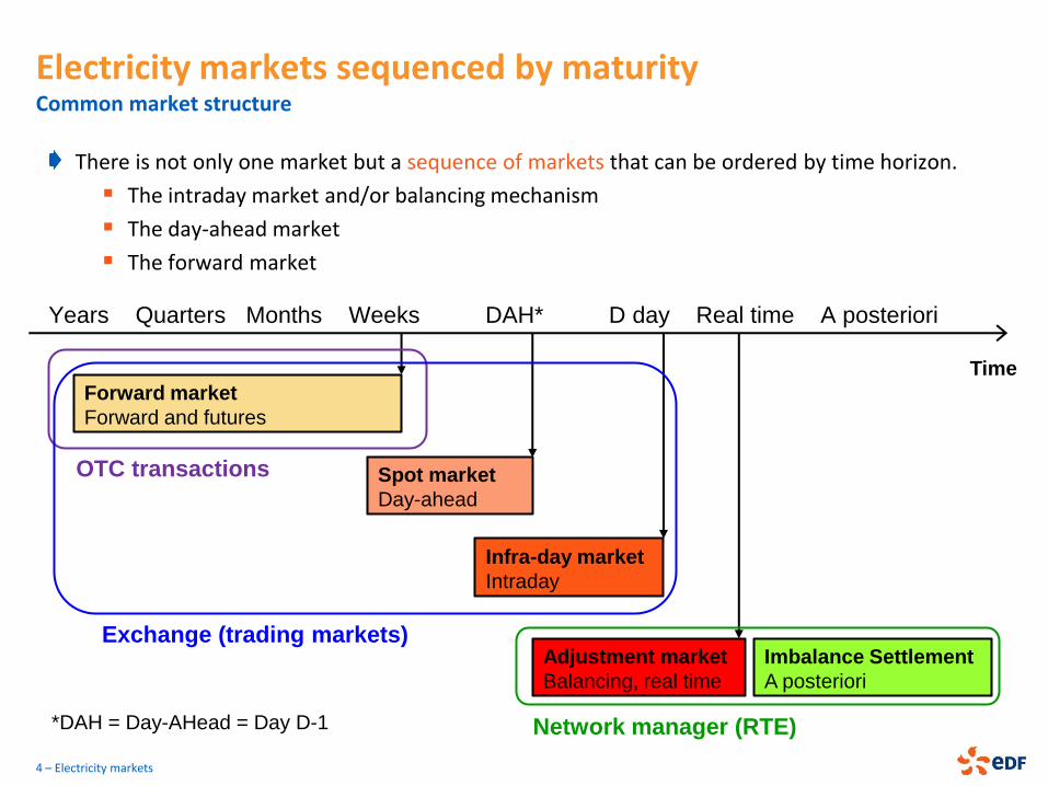
Electricity markets sequenced by maturity Common market structure
4 – Electricity markets
There is not only one market but a sequence of markets that can be ordered by time horizon.
The intraday market and/or balancing mechanism
The day-ahead market
The forward market
Time
Forward market
Forward and futures
Spot market
Day-ahead
Infra-day market
Intraday
Adjustment market
Balancing, real time
OTC transactions
Exchange (trading markets)
Network manager (RTE)
Imbalance Settlement
A posteriori
Years Quarters Months Weeks DAH* D day Real time A posteriori
*DAH = Day-AHead = Day D-1
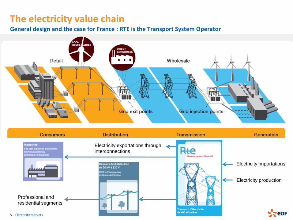
The electricity value chain General design and the case for France : RTE is the Transport System Operator
Electricity importations
Electricity production
Electricity exportations through
interconnections
Professional and
residential segments
5 – Electricity markets
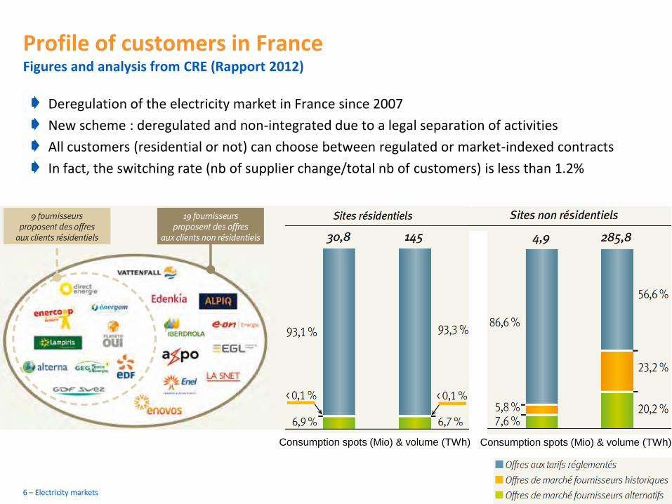
Profile of customers in France Figures and analysis from CRE (Rapport 2012)
Deregulation of the electricity market in France since 2007
New scheme : deregulated and non-integrated due to a legal separation of activities
All customers (residential or not) can choose between regulated or market-indexed contracts
In fact, the switching rate (nb of supplier change/total nb of customers) is less than 1.2%
6 – Electricity markets
Consumption spots (Mio) & volume (TWh) Consumption spots (Mio) & volume (TWh)
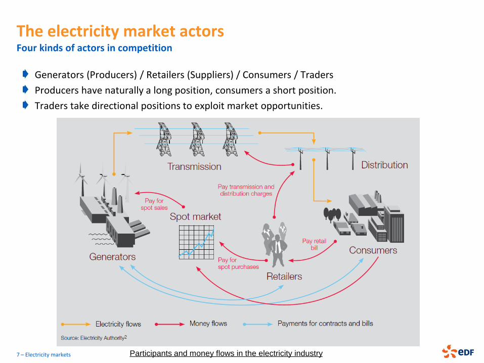
The electricity market actors Four kinds of actors in competition
Generators (Producers) / Retailers (Suppliers) / Consumers / Traders
Producers have naturally a long position, consumers a short position.
Traders take directional positions to exploit market opportunities.
7 – Electricity markets Participants and money flows in the electricity industry
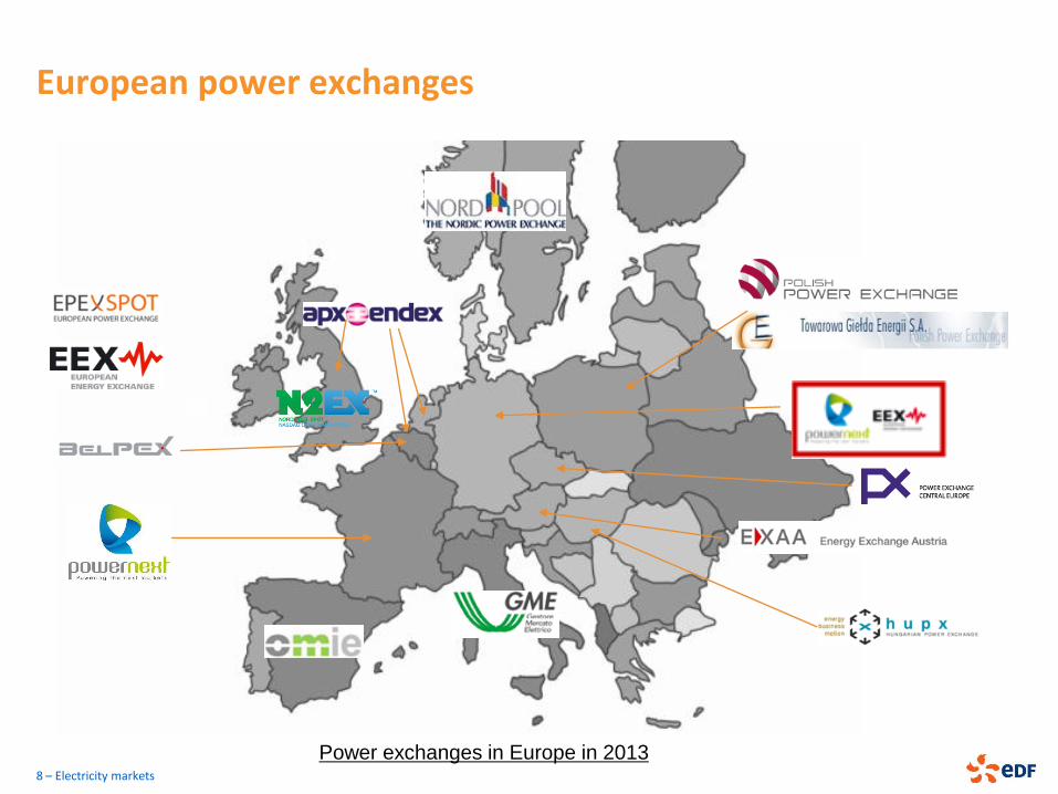
European power exchanges
8 – Electricity markets
Power exchanges in Europe in 2013
ELECTRICITY MARKET DESIGN
9 – Electricity markets
Some generalities, the electricity value chain
Electricity market microstructure
Power production tools and drivers of European electricity prices
Electricity market structure Coexistence of different markets
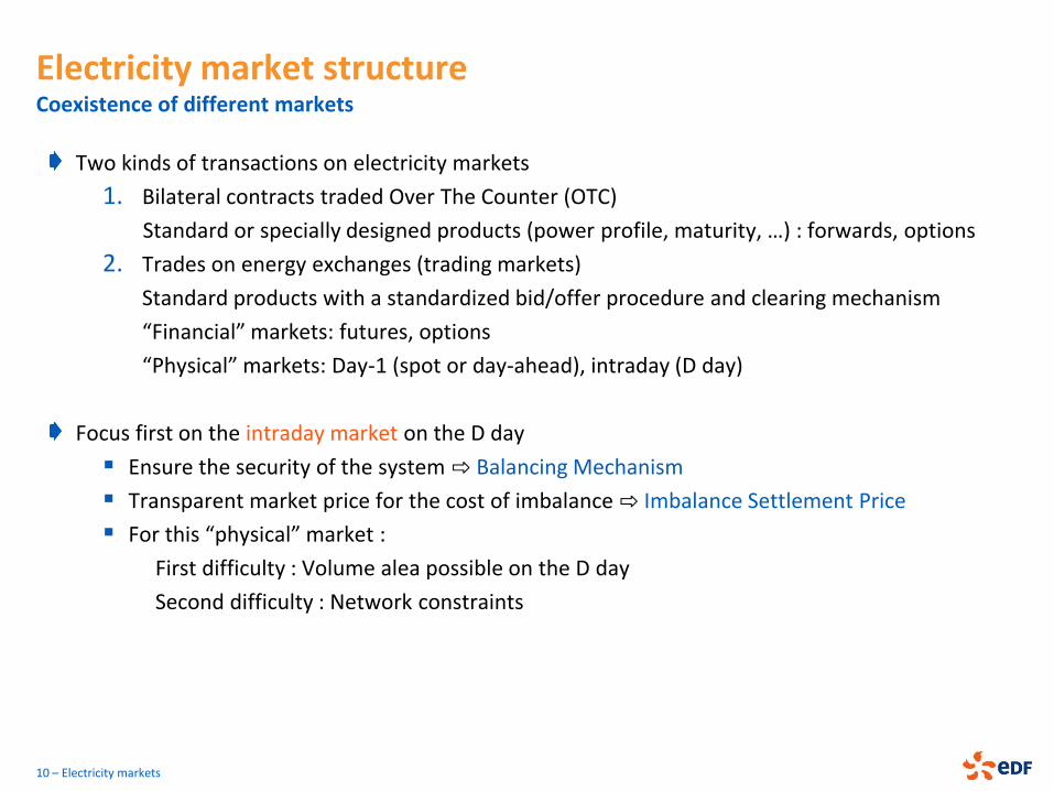
Two kinds of transactions on electricity markets
1. Bilateral contracts traded Over The Counter (OTC)
Standard or specially designed products (power profile, maturity, …) : forwards, options
2. Trades on energy exchanges (trading markets)
Standard products with a standardized bid/offer procedure and clearing mechanism
“Financial” markets: futures, options
“Physical” markets: Day-1 (spot or day-ahead), intraday (D day)
Focus first on the intraday market on the D day
Ensure the security of the system ⇨ Balancing Mechanism
Transparent market price for the cost of imbalance ⇨ Imbalance Settlement Price
For this “physical” market :
First difficulty : Volume alea possible on the D day
Second difficulty : Network constraints
10 – Electricity markets
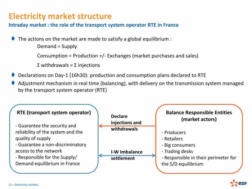
The actions on the market are made to satisfy a global equilibrium :
Demand = Supply
Consumption = Production +/- Exchanges (market purchases and sales)
Σ withdrawals = Σ injections
Declarations on Day-1 (16h30): production and consumption plans declared to RTE
Adjustment mechanism in real time (balancing), with delivery on the transmission system managed by the transport system operator (RTE)
11 – Electricity markets
RTE (transport system operator) - Guarantee the security and reliability of the system and the quality of supply - Guarantee a non-discriminatory access to the network - Responsible for the Supply/ Demand equilibrium in France
Balance Responsible Entities (market actors)
- Producers - Retailers - Big consumers - Trading desks - Responsible in their perimeter for the S/D equilibrium
Declare injections and withdrawals
I-W Imbalance settlement
Electricity market structure Intraday market : the role of the transport system operator RTE in France
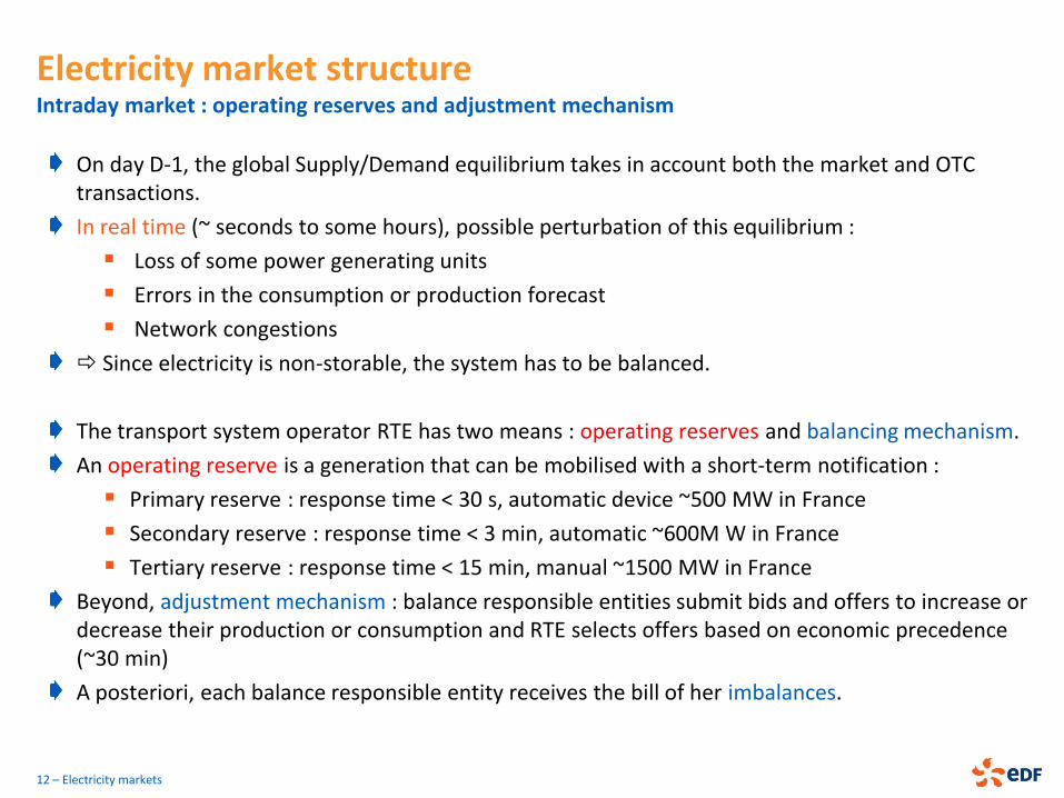
On day D-1, the global Supply/Demand equilibrium takes in account both the market and OTC transactions.
In real time (~ seconds to some hours), possible perturbation of this equilibrium :
Loss of some power generating units
Errors in the consumption or production forecast
Network congestions
Since electricity is non-storable, the system has to be balanced.
The transport system operator RTE has two means : operating reserves and balancing mechanism.
An operating reserve is a generation that can be mobilised with a short-term notification :
Primary reserve : response time < 30 s, automatic device ~500 MW in France
Secondary reserve : response time < 3 min, automatic ~600M W in France
Tertiary reserve : response time < 15 min, manual ~1500 MW in France
Beyond, adjustment mechanism : balance responsible entities submit bids and offers to increase or decrease their production or consumption and RTE selects offers based on economic precedence (~30 min)
A posteriori, each balance responsible entity receives the bill of her imbalances.
12 – Electricity markets
Electricity market structure Intraday market : operating reserves and adjustment mechanism
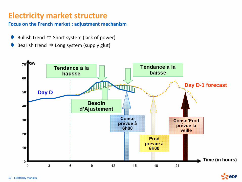
Bullish trend Short system (lack of power)
Bearish trend Long system (supply glut)
13 – Electricity markets
Day D-1 forecast
Day D
Electricity market structure Focus on the French market : adjustment mechanism
Time (in hours)
Adjustment mechanism : allow to compensate the power need/glut of the system
Bullish trend Offers for increasing the power injected (producers) in the system and erasing offers (cut-off injunctions, EJP) for reducing the demand
Bearish trend Offers for decreasing the power injected in the system (producers)
Offers ranked by merit order (RTE)
Imbalance settlement (“Règlement des écarts”)
RTE establishes, a posteriori, the bill to be paid or received by any actor, for the differentials observed on its perimeter (injections/withdrawals).
Formula based on the spot price and power generation costs
Incentive to a vertuous behavior for both producers and consumers
Example for EDF: Case of a Bull trend (lack of power)
If EDF is long (P>C) EDF receives the Spot
If EDF is short (P<C) EDF needs to pay max(Spot, Pu*)
14 – Electricity markets
*Pu = upper weighted average cost of power generation issued from the adjustment mechanism
Electricity market structure Focus on the French market : adjustment mechanism and imbalance settlement
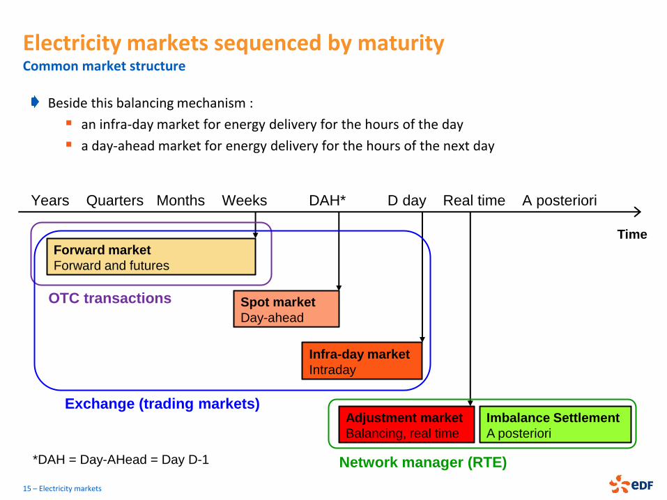
Electricity markets sequenced by maturity Common market structure
15 – Electricity markets
Beside this balancing mechanism :
an infra-day market for energy delivery for the hours of the day
a day-ahead market for energy delivery for the hours of the next day
Time
Forward market
Forward and futures
Spot market
Day-ahead
Infra-day market
Intraday
Adjustment market
Balancing, real time
OTC transactions
Exchange (trading markets)
Network manager (RTE)
Imbalance Settlement
A posteriori
Years Quarters Months Weeks DAH* D day Real time A posteriori
*DAH = Day-AHead = Day D-1
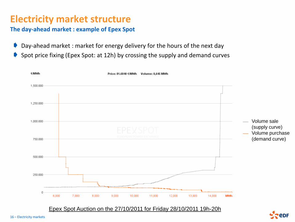
Electricity market structure The day-ahead market : example of Epex Spot
Day-ahead market : market for energy delivery for the hours of the next day
Spot price fixing (Epex Spot: at 12h) by crossing the supply and demand curves
16 – Electricity markets
Volume sale
(supply curve)
Volume purchase
(demand curve)
Epex Spot Auction on the 27/10/2011 for Friday 28/10/2011 19h-20h
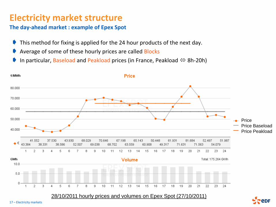
This method for fixing is applied for the 24 hour products of the next day.
Average of some of these hourly prices are called Blocks
In particular, Baseload and Peakload prices (in France, Peakload 8h-20h)
17 – Electricity markets
28/10/2011 hourly prices and volumes on Epex Spot (27/10/2011)
Price
Price Baseload
Price Peakload
Electricity market structure The day-ahead market : example of Epex Spot
18 – Electricity markets
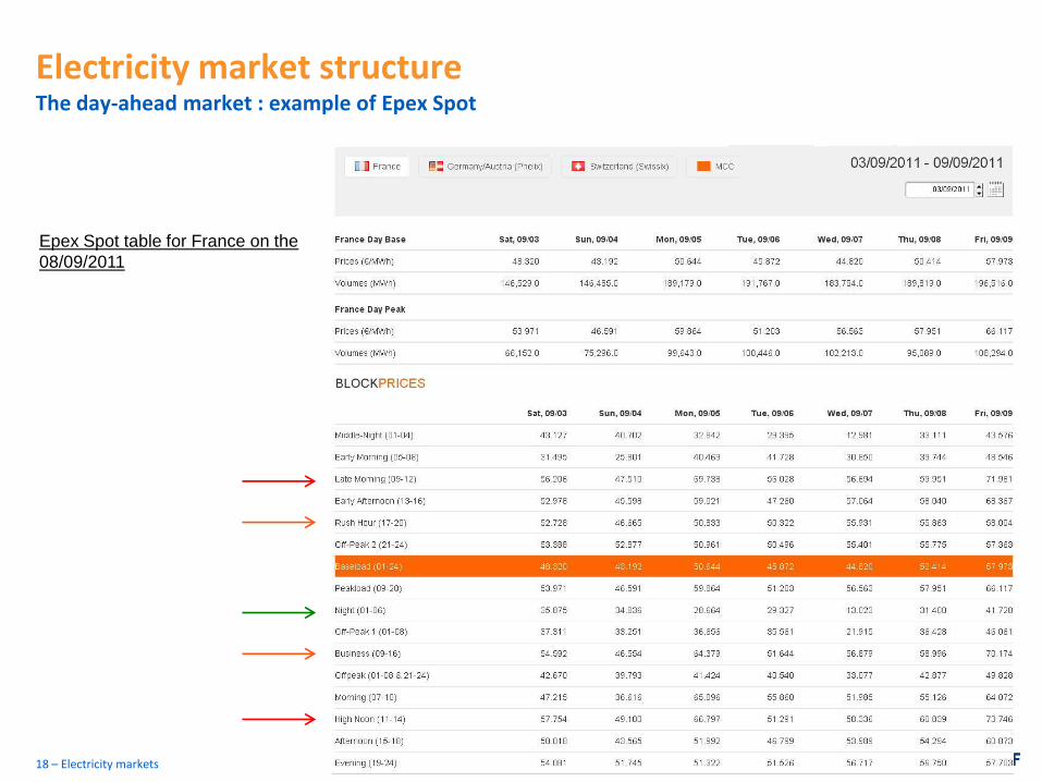
Epex Spot table for France on the
08/09/2011
Electricity market structure The day-ahead market : example of Epex Spot
Electricity market structure The forward market
19 – Electricity markets
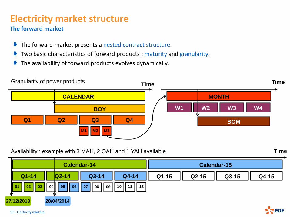
The forward market presents a nested contract structure.
Two basic characteristics of forward products : maturity and granularity.
The availability of forward products evolves dynamically.
Time
CALENDAR
Q1 Q2 Q3 Q4
M1 M2 M3
Calendar-14 Calendar-15
Q1-14 Q2-14 Q3-14 Q4-14
04 05 06 01 02 03
27/12/2013
07 08 09
Q1-15 Q2-15 Q3-15 Q4-15
MONTH
W1 W2 W3 W4
BOM
BOY
Time
28/04/2014
Time
10 11 12
Availability : example with 3 MAH, 2 QAH and 1 YAH available
Granularity of power products
20 – Electricity markets
The forward market corresponds to the market for products with granularities and maturities greater than one day.
Example of EEX : are available at the same time the following forward products :
6 calendars
11 quarters
9 months
4 weeks
2 weekends
8 days
In three flavours : Baseload (each hour), Peakload (8h-20h Monday to Friday) and Offpeak
Thus, 106 contracts are available… to be compared to the 525684 hours in the next six years…
Electricity market structure The forward market
Market horizon : Last delivery date covered by the futures products quoted Market depth : Available volumes of tradable products Completeness : Ability to find products on for any market horizons and any granularity
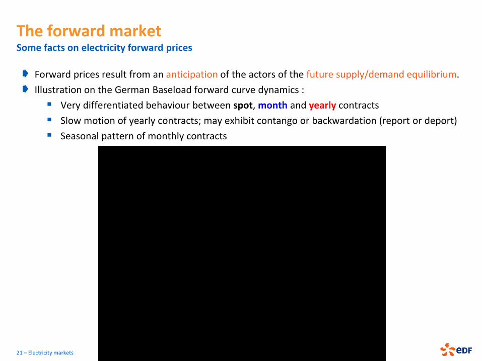
The forward market Some facts on electricity forward prices
Forward prices result from an anticipation of the actors of the future supply/demand equilibrium.
Illustration on the German Baseload forward curve dynamics :
Very differentiated behaviour between spot, month and yearly contracts
Slow motion of yearly contracts; may exhibit contango or backwardation (report or deport)
Seasonal pattern of monthly contracts
21 – Electricity markets
22 – Electricity markets
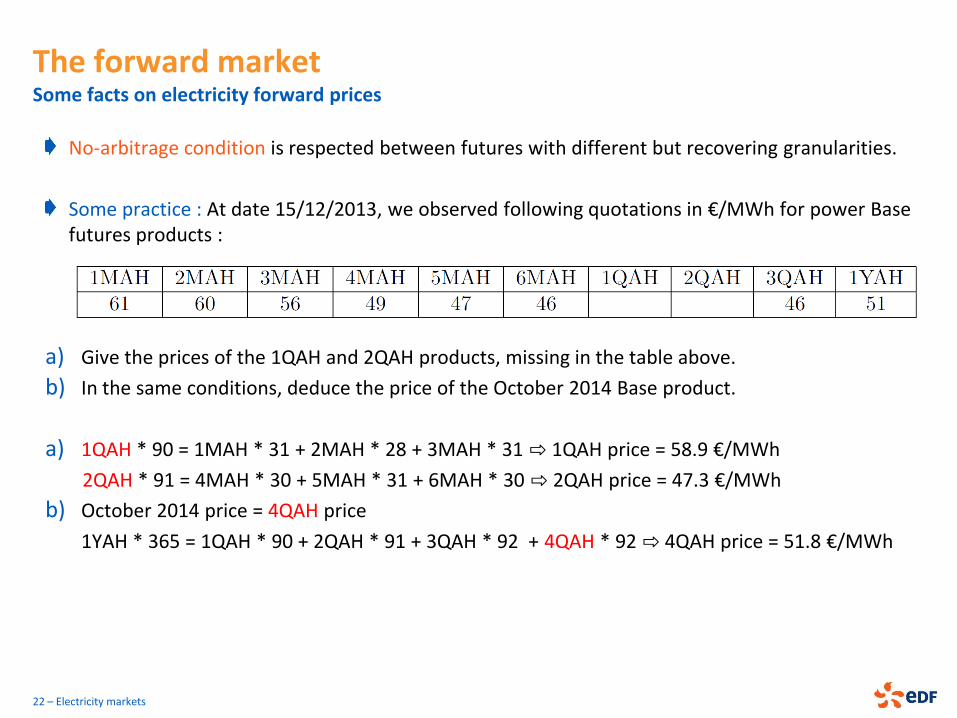
No-arbitrage condition is respected between futures with different but recovering granularities.
Some practice : At date 15/12/2013, we observed following quotations in €/MWh for power Base futures products :
a) Give the prices of the 1QAH and 2QAH products, missing in the table above.
b) In the same conditions, deduce the price of the October 2014 Base product.
a) 1QAH * 90 = 1MAH * 31 + 2MAH * 28 + 3MAH * 31 ⇨ 1QAH price = 58.9 €/MWh
2QAH * 91 = 4MAH * 30 + 5MAH * 31 + 6MAH * 30 ⇨ 2QAH price = 47.3 €/MWh
b) October 2014 price = 4QAH price
1YAH * 365 = 1QAH * 90 + 2QAH * 91 + 3QAH * 92 + 4QAH * 92 ⇨ 4QAH price = 51.8 €/MWh
The forward market Some facts on electricity forward prices
23 – Electricity markets
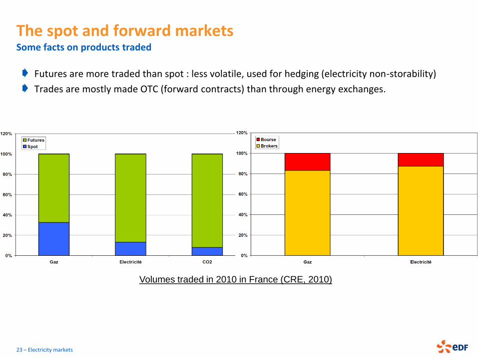
Futures are more traded than spot : less volatile, used for hedging (electricity non-storability)
Trades are mostly made OTC (forward contracts) than through energy exchanges.
The spot and forward markets Some facts on products traded
Volumes traded in 2010 in France (CRE, 2010)
ELECTRICITY MARKET DESIGN
24 – Electricity markets
Some generalities, the electricity value chain
Electricity market microstructure
Power production tools and drivers of European electricity prices
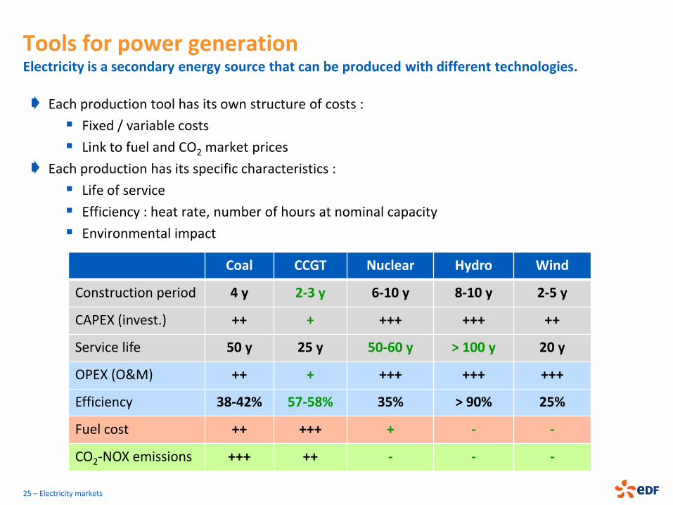
Tools for power generation Electricity is a secondary energy source that can be produced with different technologies.
25 – Electricity markets
Coal CCGT Nuclear Hydro Wind
Construction period 4 y 2-3 y 6-10 y 8-10 y 2-5 y
CAPEX (invest.) ++ + +++ +++ ++
Service life 50 y 25 y 50-60 y > 100 y 20 y
OPEX (O&M) ++ + +++ +++ +++
Efficiency 38-42% 57-58% 35% > 90% 25%
Fuel cost ++ +++ + - -
CO2-NOX emissions +++ ++ - - -
Each production tool has its own structure of costs :
Fixed / variable costs
Link to fuel and CO2 market prices
Each production has its specific characteristics :
Life of service
Efficiency : heat rate, number of hours at nominal capacity
Environmental impact
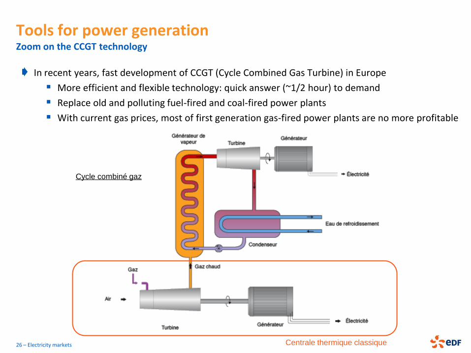
Tools for power generation Zoom on the CCGT technology
In recent years, fast development of CCGT (Cycle Combined Gas Turbine) in Europe
More efficient and flexible technology: quick answer (~1/2 hour) to demand
Replace old and polluting fuel-fired and coal-fired power plants
With current gas prices, most of first generation gas-fired power plants are no more profitable
26 – Electricity markets Centrale thermique classique
Cycle combiné gaz
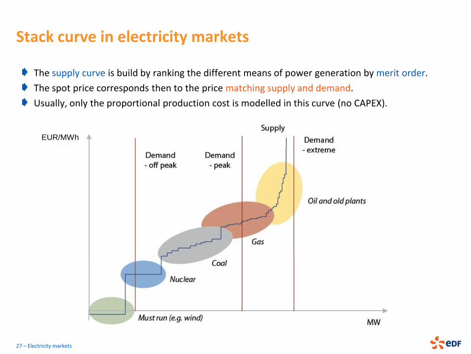
Stack curve in electricity markets
The supply curve is build by ranking the different means of power generation by merit order.
The spot price corresponds then to the price matching supply and demand.
Usually, only the proportional production cost is modelled in this curve (no CAPEX).
27 – Electricity markets
EUR/MWh
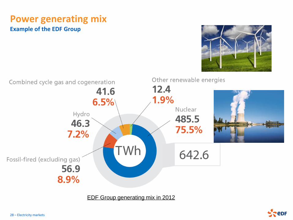
Power generating mix Example of the EDF Group
28 – Electricity markets
EDF Group generating mix in 2012
29 – Electricity markets
Source: Enerdata
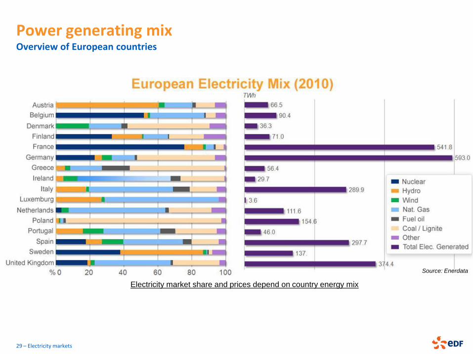
Electricity market share and prices depend on country energy mix
Power generating mix Overview of European countries
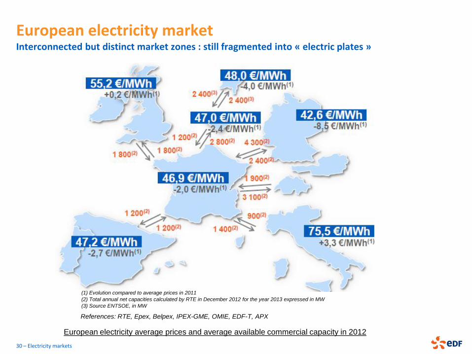
European electricity market Interconnected but distinct market zones : still fragmented into « electric plates »
30 – Electricity markets
(1) Evolution compared to average prices in 2011
(2) Total annual net capacities calculated by RTE in December 2012 for the year 2013 expressed in MW
(3) Source ENTSOE, in MW
European electricity average prices and average available commercial capacity in 2012
References: RTE, Epex, Belpex, IPEX-GME, OMIE, EDF-T, APX
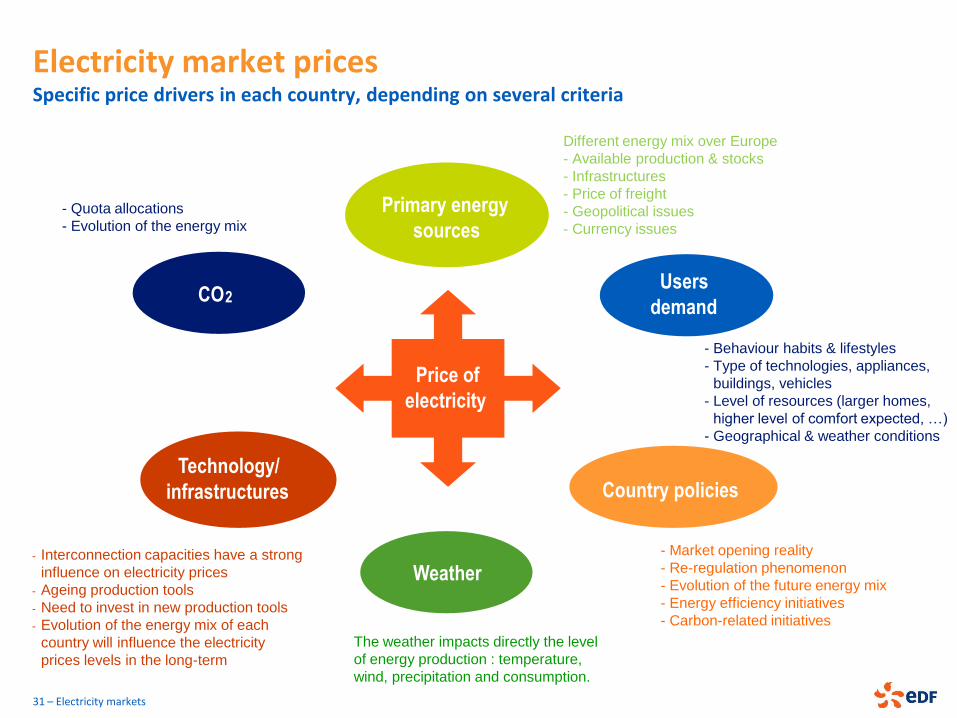
Electricity market prices Specific price drivers in each country, depending on several criteria
31 – Electricity markets
- Market opening reality
- Re-regulation phenomenon
- Evolution of the future energy mix
- Energy efficiency initiatives
- Carbon-related initiatives
The weather impacts directly the level
of energy production : temperature,
wind, precipitation and consumption.
- Interconnection capacities have a strong
influence on electricity prices
- Ageing production tools
- Need to invest in new production tools
- Evolution of the energy mix of each
country will influence the electricity
prices levels in the long-term
Different energy mix over Europe
- Available production & stocks
- Infrastructures
- Price of freight
- Geopolitical issues
- Currency issues
- Behaviour habits & lifestyles
- Type of technologies, appliances,
buildings, vehicles
- Level of resources (larger homes,
higher level of comfort expected, …)
- Geographical & weather conditions
- Quota allocations
- Evolution of the energy mix
CO 2
Primary energy
sources
Country policies
Weather
Technology/
infrastructures
Price of
electricity
Users
demand
Electricity market : main challenges
Key factors are changing the world :
An increase in the urban population: 50% of people living in cities, 70% by 2050
Resource scarcity
The need to “decarbonise” energy
A plural and multi-polar world (new emerging powers: China, Brazil, India, etc.)
An ever-more sprawling, decentralised world (urban systems, local energies, smart grids, etc.)
Today, the energy markets are facing a difficult equation :
Reduction of available resources : oil, gas, ...
Ageing production assets : nuclear power plants, ...
Environmental issues
An increasing demand
Precise forecasting are risky. Too many factors can influence the prices...
Tomorrow, the energy world will be even more uncertain and volatile.
32 – Electricity markets
MODELLING ELECTRICITY PRICES
33 – Electricity markets
Main features of power spot prices
Overview of spot and forward models
A structural model for electricity prices (Aïd et al., 2011)
Factorial models for energy prices (e.g. Kiesel et al., 2008)
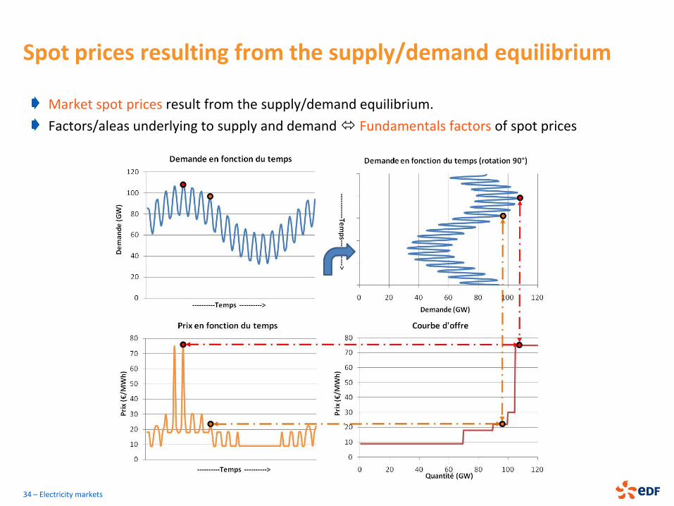
Spot prices resulting from the supply/demand equilibrium
Market spot prices result from the supply/demand equilibrium.
Factors/aleas underlying to supply and demand Fundamentals factors of spot prices
34 – Electricity markets
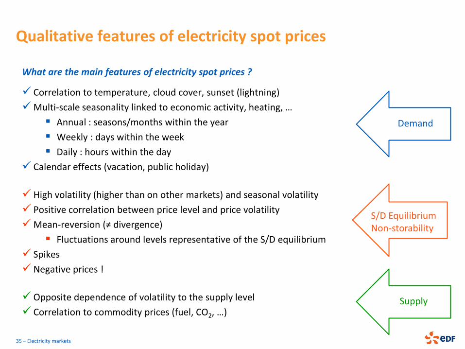
Qualitative features of electricity spot prices
What are the main features of electricity spot prices ?
Correlation to temperature, cloud cover, sunset (lightning)
Multi-scale seasonality linked to economic activity, heating, …
Annual : seasons/months within the year
Weekly : days within the week
Daily : hours within the day
Calendar effects (vacation, public holiday)
High volatility (higher than on other markets) and seasonal volatility
Positive correlation between price level and price volatility
Mean-reversion (≠ divergence)
Fluctuations around levels representative of the S/D equilibrium
Spikes
Negative prices !
Opposite dependence of volatility to the supply level
Correlation to commodity prices (fuel, CO2, …)
35 – Electricity markets
Demand
S/D Equilibrium Non-storability
Supply
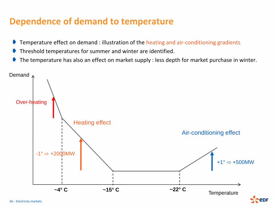
Dependence of demand to temperature
Temperature effect on demand : illustration of the heating and air-conditioning gradients
Threshold temperatures for summer and winter are identified.
The temperature has also an effect on market supply : less depth for market purchase in winter.
36 – Electricity markets
Temperature
Demand
+1° ⇨ +500MW
-1° ⇨ +2000MW
Air-conditioning effect
Heating effect
Over-heating
~4° C ~15° C ~22° C
Seasonality of electricity spot prices
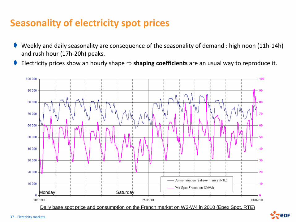
Weekly and daily seasonality are consequence of the seasonality of demand : high noon (11h-14h) and rush hour (17h-20h) peaks.
Electricity prices show an hourly shape ⇨ shaping coefficients are an usual way to reproduce it.
37 – Electricity markets
Monday Saturday
Daily base spot price and consumption on the French market on W3-W4 in 2010 (Epex Spot, RTE)
Shaping coefficients for electricity spot prices
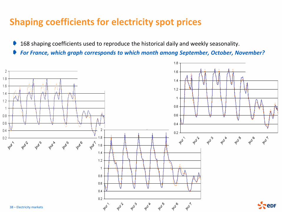
168 shaping coefficients used to reproduce the historical daily and weekly seasonality.
For France, which graph corresponds to which month among September, October, November?
38 – Electricity markets
Shaping coefficients for electricity spot prices
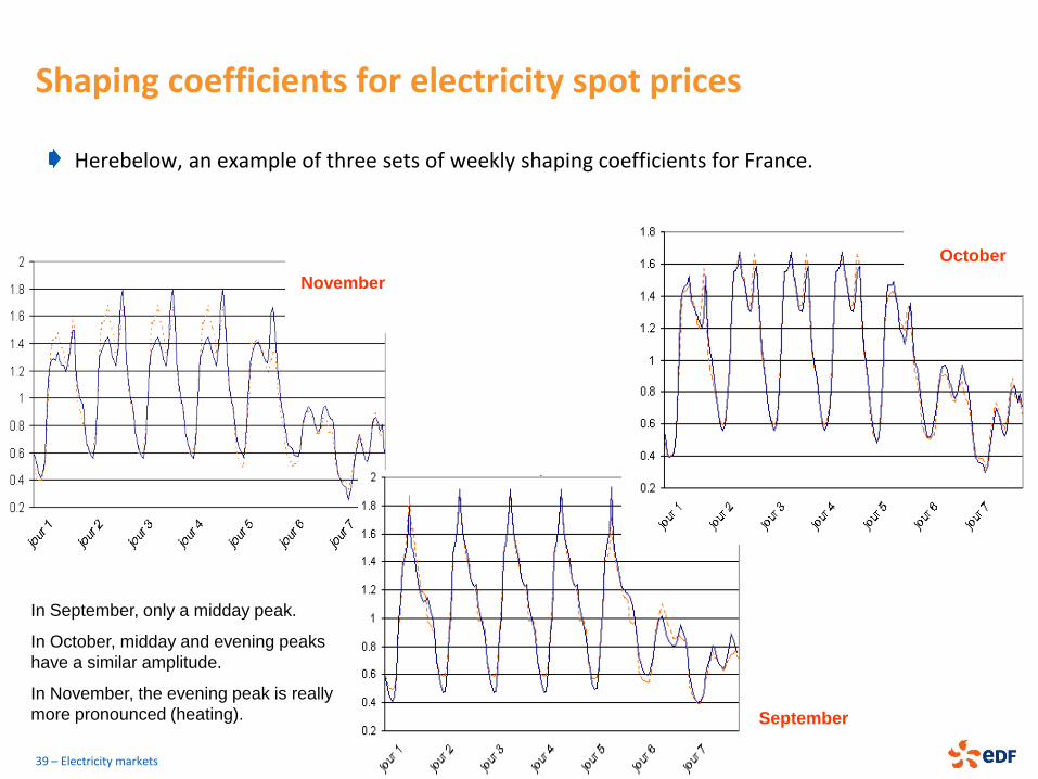
Herebelow, an example of three sets of weekly shaping coefficients for France.
39 – Electricity markets
In September, only a midday peak.
In October, midday and evening peaks
have a similar amplitude.
In November, the evening peak is really
more pronounced (heating). September
November
October
Mean reverting behavior of electricity spot prices
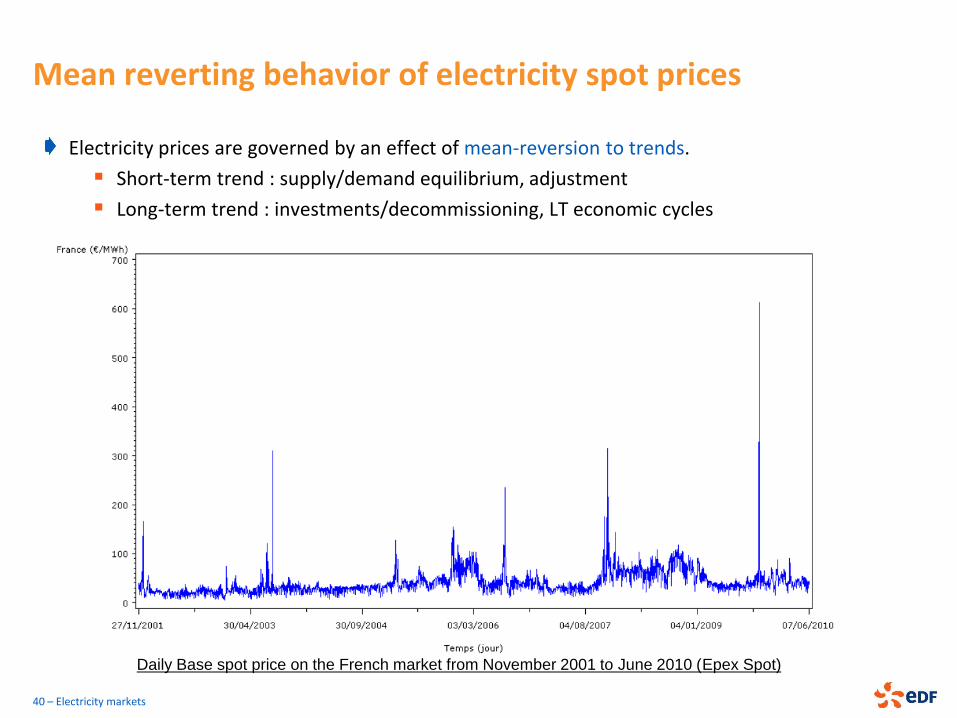
Electricity prices are governed by an effect of mean-reversion to trends.
Short-term trend : supply/demand equilibrium, adjustment
Long-term trend : investments/decommissioning, LT economic cycles
40 – Electricity markets
Daily Base spot price on the French market from November 2001 to June 2010 (Epex Spot)
Electricity prices spikes
41 – Electricity markets
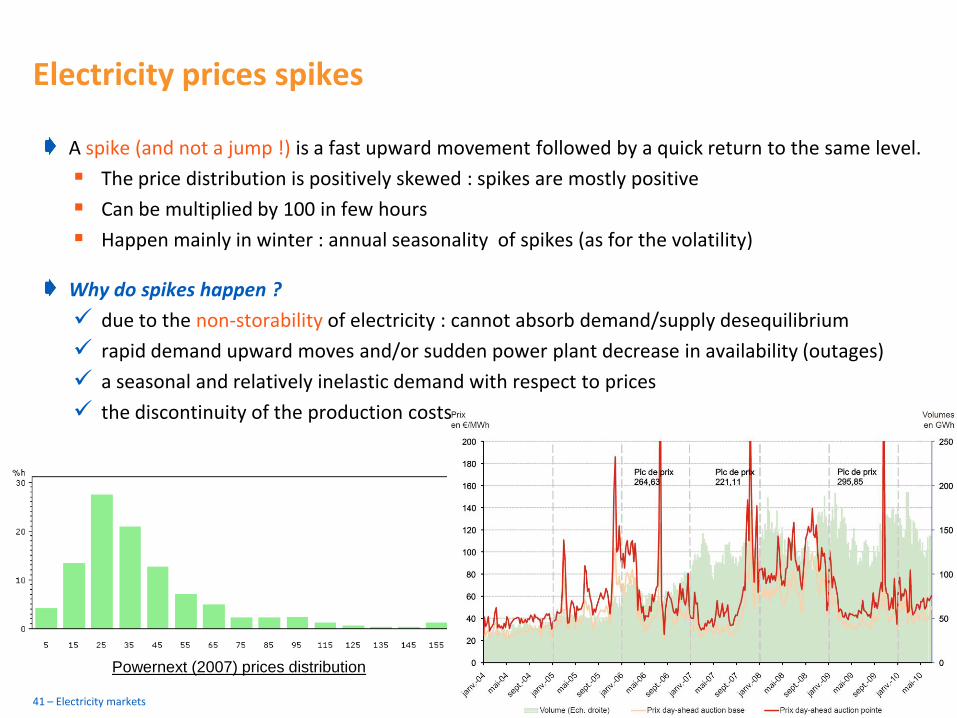
Powernext (2007) prices distribution
A spike (and not a jump !) is a fast upward movement followed by a quick return to the same level.
The price distribution is positively skewed : spikes are mostly positive
Can be multiplied by 100 in few hours
Happen mainly in winter : annual seasonality of spikes (as for the volatility)
Why do spikes happen ?
due to the non-storability of electricity : cannot absorb demand/supply desequilibrium
rapid demand upward moves and/or sudden power plant decrease in availability (outages)
a seasonal and relatively inelastic demand with respect to prices
the discontinuity of the production costs
Electricity prices spikes due to a very high demand
42 – Electricity markets
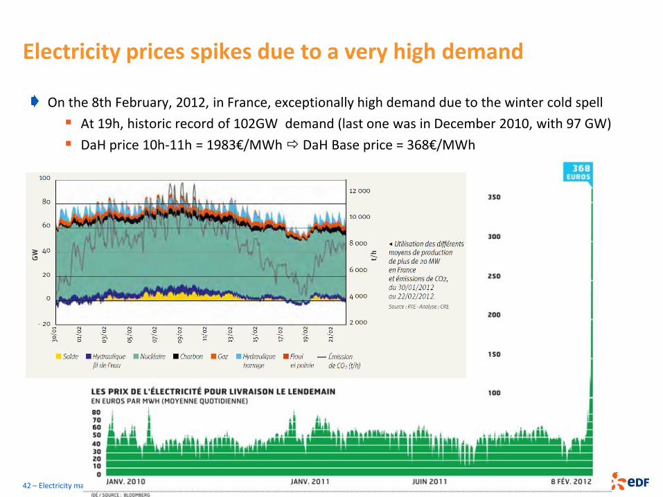
On the 8th February, 2012, in France, exceptionally high demand due to the winter cold spell
At 19h, historic record of 102GW demand (last one was in December 2010, with 97 GW)
DaH price 10h-11h = 1983€/MWh DaH Base price = 368€/MWh
Prices spikes due to a supply/demand desequilibrium
43 – Electricity markets
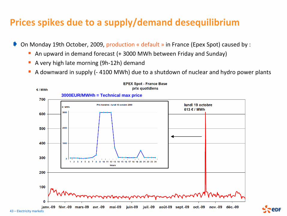
On Monday 19th October, 2009, production « default » in France (Epex Spot) caused by :
An upward in demand forecast (+ 3000 MWh between Friday and Sunday)
A very high late morning (9h-12h) demand
A downward in supply (- 4100 MWh) due to a shutdown of nuclear and hydro power plants
3000EUR/MWHh = Technical max price
Negative electricity spot prices
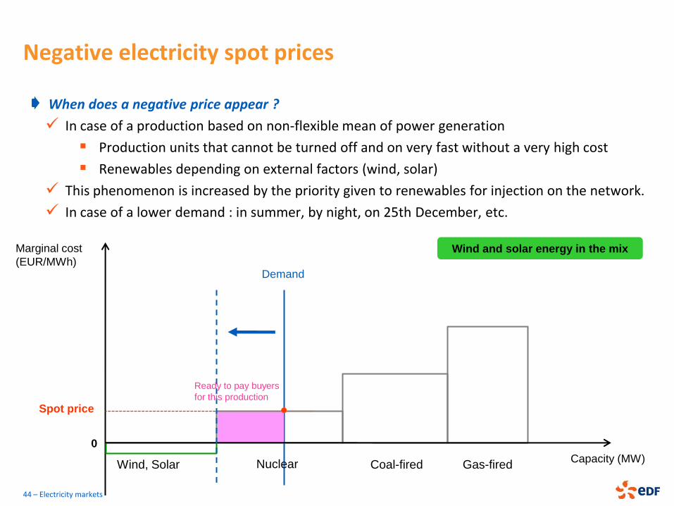
When does a negative price appear ?
In case of a production based on non-flexible mean of power generation
Production units that cannot be turned off and on very fast without a very high cost
Renewables depending on external factors (wind, solar)
This phenomenon is increased by the priority given to renewables for injection on the network.
In case of a lower demand : in summer, by night, on 25th December, etc.
Wind, Solar Capacity (MW)
Marginal cost
(EUR/MWh)
Coal-fired Gas-fired
Spot price
Wind and solar energy in the mix
Demand
Nuclear
Ready to pay buyers
for this production
0
44 – Electricity markets
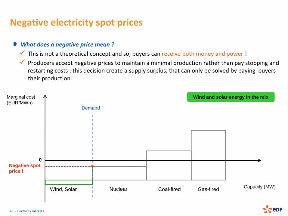
Negative electricity spot prices
What does a negative price mean ?
This is not a theoretical concept and so, buyers can receive both money and power !
Producers accept negative prices to maintain a minimal production rather than pay stopping and restarting costs : this decision create a supply surplus, that can only be solved by paying buyers their production.
Wind, Solar Capacity (MW)
Marginal cost
(EUR/MWh)
Coal-fired Gas-fired
Negative spot
price !
Wind and solar energy in the mix
Nuclear
0
Demand
45 – Electricity markets
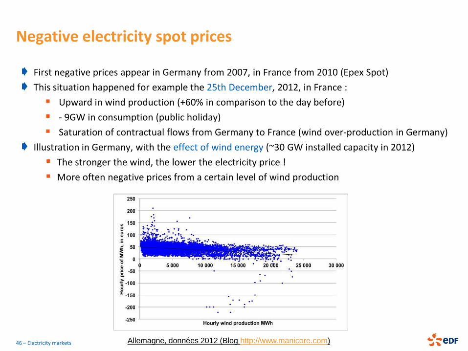
Negative electricity spot prices
First negative prices appear in Germany from 2007, in France from 2010 (Epex Spot)
This situation happened for example the 25th December, 2012, in France :
Upward in wind production (+60% in comparison to the day before)
- 9GW in consumption (public holiday)
Saturation of contractual flows from Germany to France (wind over-production in Germany)
Illustration in Germany, with the effect of wind energy (~30 GW installed capacity in 2012)
The stronger the wind, the lower the electricity price !
More often negative prices from a certain level of wind production
46 – Electricity markets Allemagne, données 2012 (Blog http://www.manicore.com)
MODELLING ELECTRICITY PRICES
47 – Electricity markets
Main features of power forward prices
Overview of spot and forward models
A structural model for electricity prices (Aïd et al., 2011)
Factorial models for energy prices
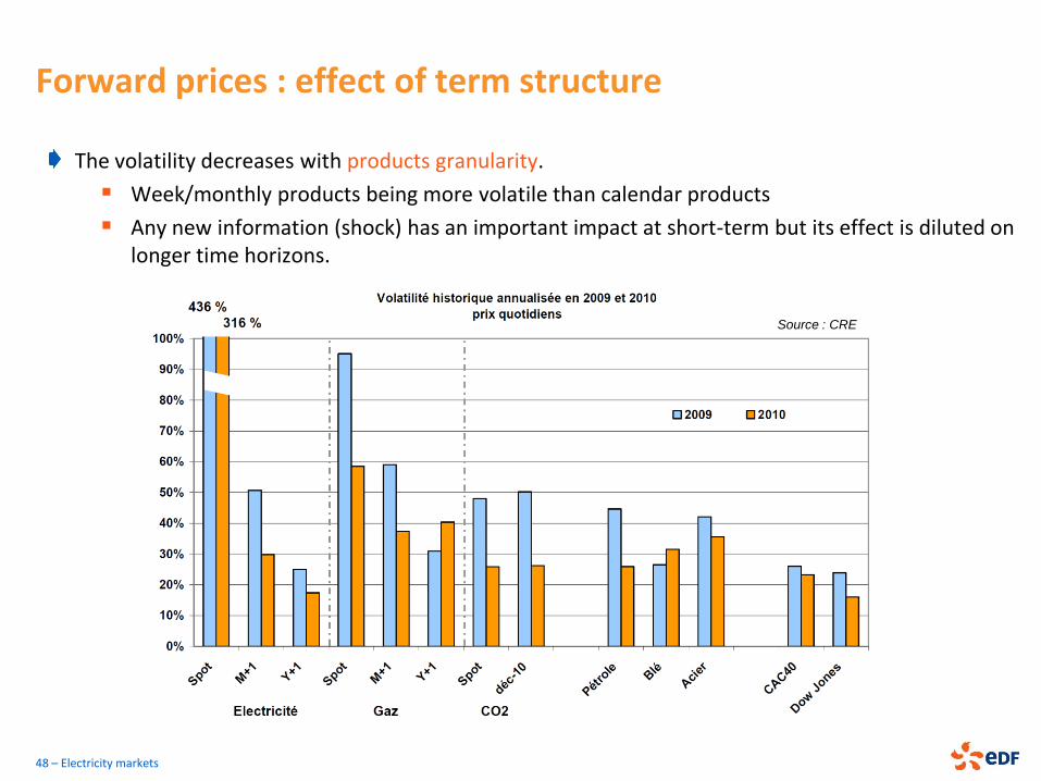
Forward prices : effect of term structure
The volatility decreases with products granularity.
Week/monthly products being more volatile than calendar products
Any new information (shock) has an important impact at short-term but its effect is diluted on longer time horizons.
48 – Electricity markets
Source : CRE
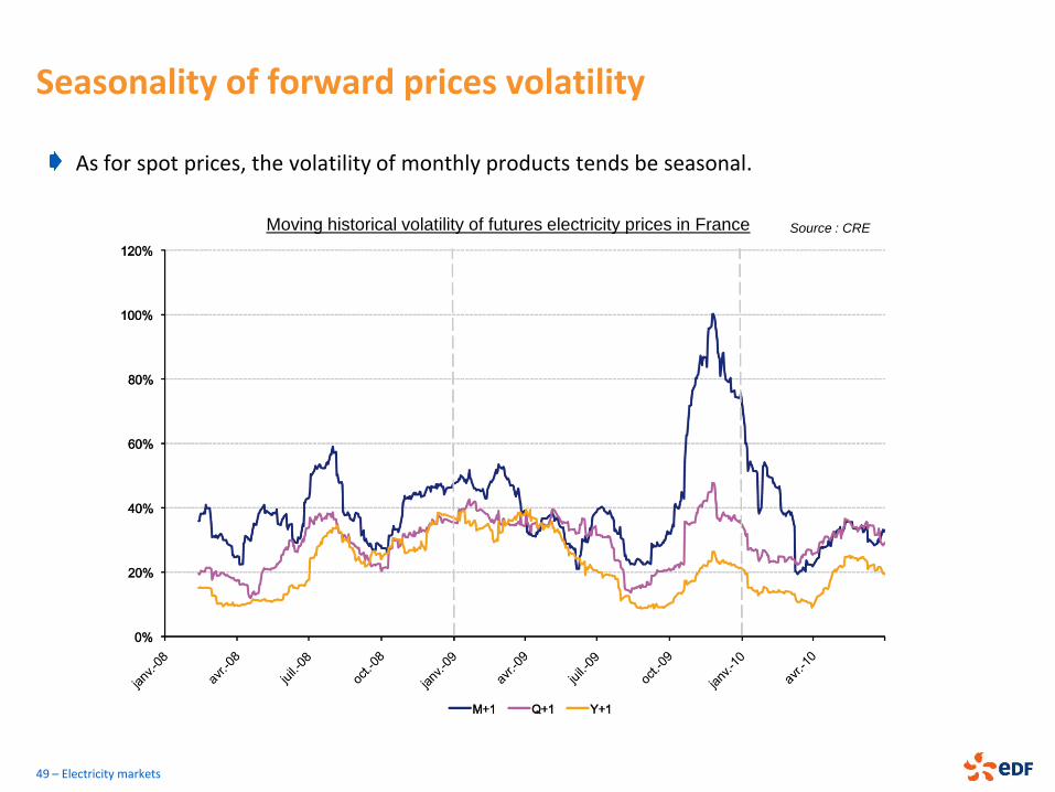
Seasonality of forward prices volatility
As for spot prices, the volatility of monthly products tends be seasonal.
49 – Electricity markets
Moving historical volatility of futures electricity prices in France Source : CRE
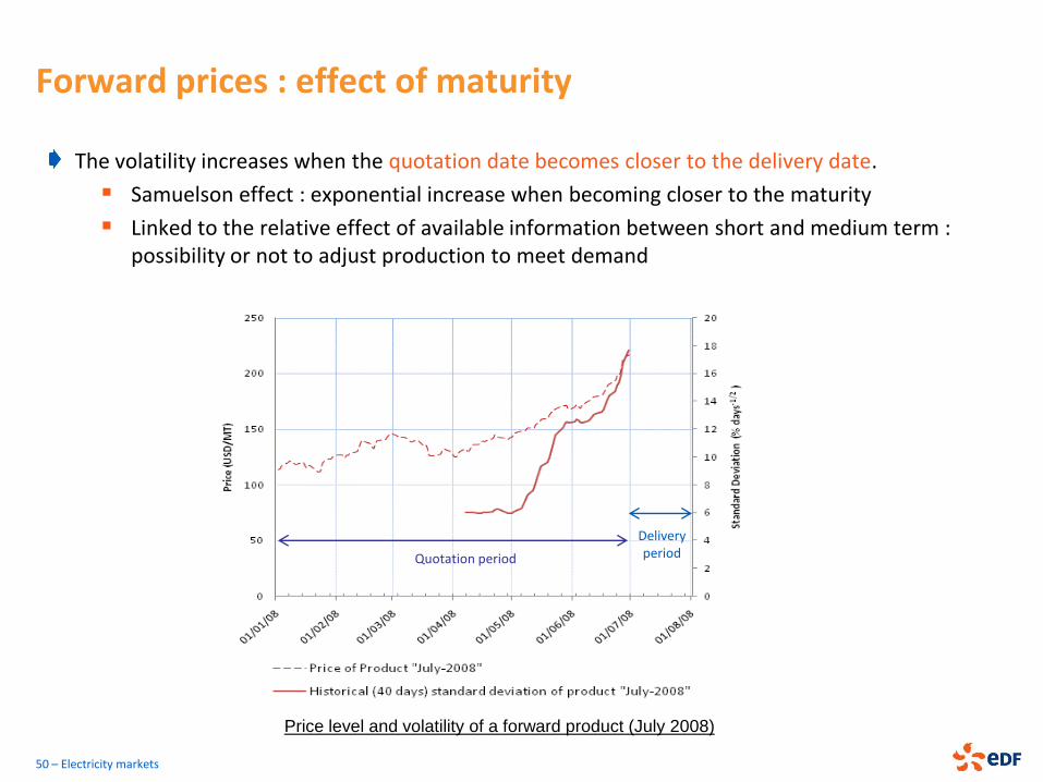
Forward prices : effect of maturity
The volatility increases when the quotation date becomes closer to the delivery date.
Samuelson effect : exponential increase when becoming closer to the maturity
Linked to the relative effect of available information between short and medium term : possibility or not to adjust production to meet demand
50 – Electricity markets
Price level and volatility of a forward product (July 2008)
Quotation period
Delivery period
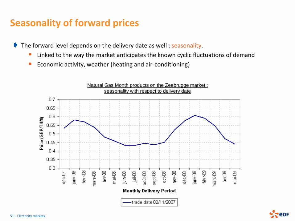
Seasonality of forward prices
The forward level depends on the delivery date as well : seasonality.
Linked to the way the market anticipates the known cyclic fluctuations of demand
Economic activity, weather (heating and air-conditioning)
51 – Electricity markets
Natural Gas Month products on the Zeebrugge market :
seasonality with respect to delivery date
MODELLING ELECTRICITY PRICES
52 – Electricity markets
Main features of power forward prices
Overview of spot and forward models
A structural model for electricity prices (Aïd et al., 2011)
Factorial models for energy prices
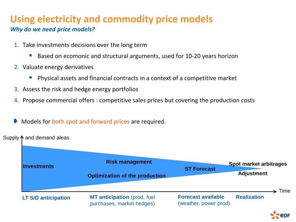
Using electricity and commodity price models Why do we need price models?
1. Take investments decisions over the long term
Based on ecomonic and structural arguments, used for 10-20 years horizon
2. Valuate energy derivatives
Physical assets and financial contracts in a context of a competitive market
3. Assess the risk and hedge energy portfolios
4. Propose commercial offers : competitive sales prices but covering the production costs
Models for both spot and forward prices are required.
Investments
Optimization of the production
ST Forecast Adjustment
Risk management Spot market arbitrages
Time
Supply and demand aleas
Forecast available
(weather, power prod) LT S/D anticipation Realization MT anticipation (prod, fuel
purchases, market hedges)
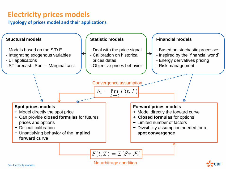
Electricity prices models Typology of prices model and their applications
54 – Electricity markets
Stuctural models
- Models based on the S/D E
- Integrating exogenous variables
- LT applicatons
- ST forecast : Spot = Marginal cost
Financial models
- Based on stochastic processes
- Inspired by the “financial world”
- Energy derivatives pricing
- Risk management
Statistic models
- Deal with the price signal
- Calibration on historical
prices datas
- Objective prices behavior
Spot prices models
+ Model directly the spot price
+ Can provide closed formulas for futures
prices and options
− Difficult calibration
− Unsatisfying behavior of the implied
forward curve
Forward prices models
+ Model directly the forward curve
+ Closed formulas for options
− Limited number of factors
− Divisibility assumption needed for a
spot convergence
Convergence assumption
No-arbitrage condition
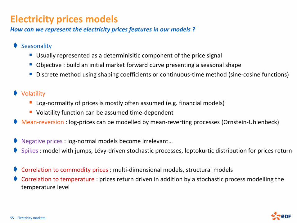
Electricity prices models How can we represent the electricity prices features in our models ?
Seasonality
Usually represented as a determinisitic component of the price signal
Objective : build an initial market forward curve presenting a seasonal shape
Discrete method using shaping coefficients or continuous-time method (sine-cosine functions)
Volatility
Log-normality of prices is mostly often assumed (e.g. financial models)
Volatility function can be assumed time-dependent
Mean-reversion : log-prices can be modelled by mean-reverting processes (Ornstein-Uhlenbeck)
Negative prices : log-normal models become irrelevant…
Spikes : model with jumps, Lévy-driven stochastic processes, leptokurtic distribution for prices return
Correlation to commodity prices : multi-dimensional models, structural models
Correlation to temperature : prices return driven in addition by a stochastic process modelling the temperature level
55 – Electricity markets
MODELLING ELECTRICITY PRICES
56 – Electricity markets
Main features of power forward prices
Overview of spot and forward models
A structural model for electricity prices (Aïd et al., 2011)
Factorial models for energy prices
A structural model for electricity prices (Aïd et al., 2011)
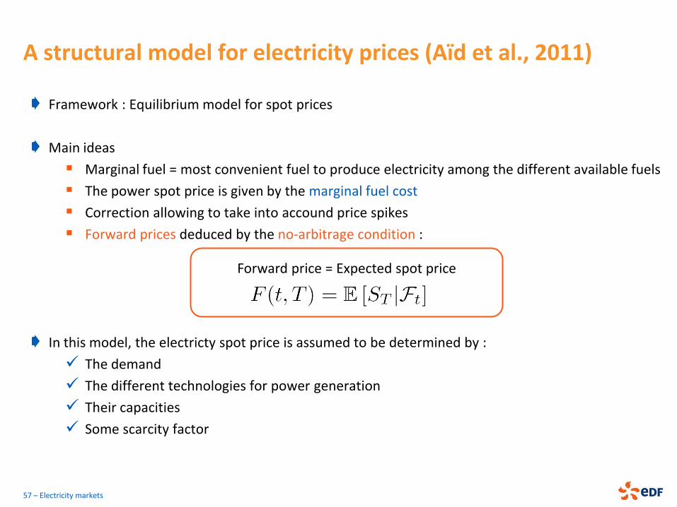
Framework : Equilibrium model for spot prices
Main ideas
Marginal fuel = most convenient fuel to produce electricity among the different available fuels
The power spot price is given by the marginal fuel cost
Correction allowing to take into accound price spikes
Forward prices deduced by the no-arbitrage condition :
In this model, the electricty spot price is assumed to be determined by :
The demand
The different technologies for power generation
Their capacities
Some scarcity factor
57 – Electricity markets
Forward price = Expected spot price
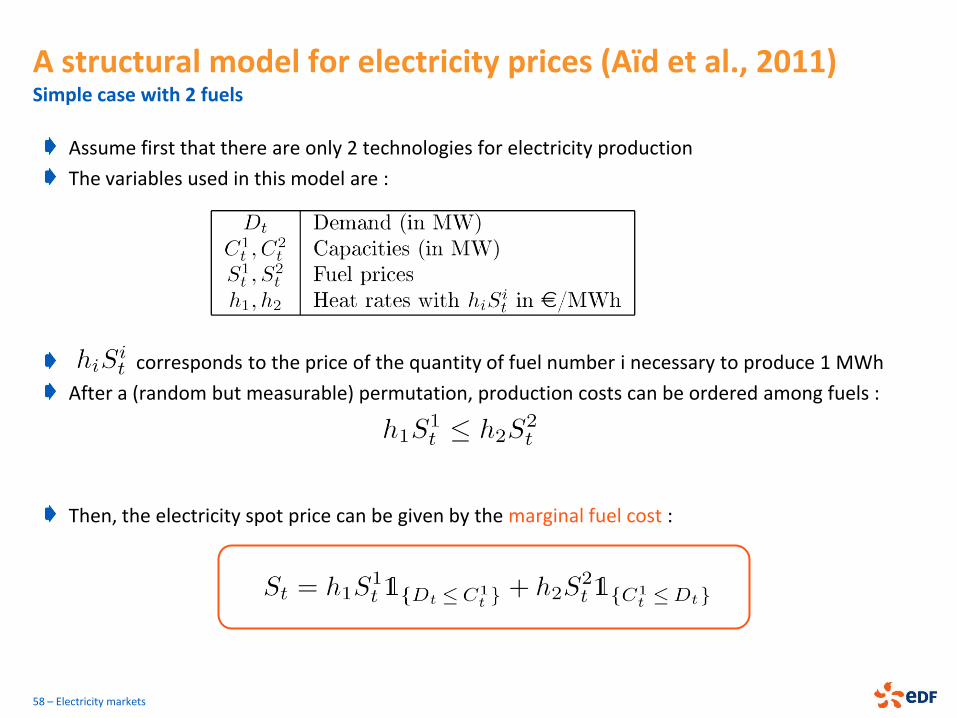
A structural model for electricity prices (Aïd et al., 2011) Simple case with 2 fuels
Assume first that there are only 2 technologies for electricity production
The variables used in this model are :
corresponds to the price of the quantity of fuel number i necessary to produce 1 MWh
After a (random but measurable) permutation, production costs can be ordered among fuels :
Then, the electricity spot price can be given by the marginal fuel cost :
58 – Electricity markets
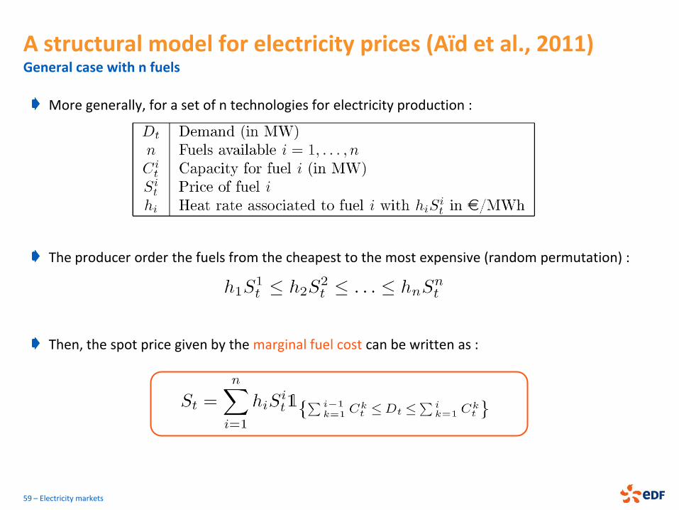
A structural model for electricity prices (Aïd et al., 2011) General case with n fuels
More generally, for a set of n technologies for electricity production :
The producer order the fuels from the cheapest to the most expensive (random permutation) :
Then, the spot price given by the marginal fuel cost can be written as :
59 – Electricity markets
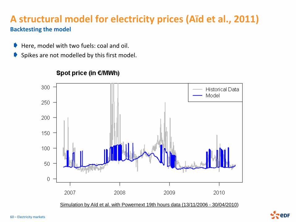
A structural model for electricity prices (Aïd et al., 2011) Backtesting the model
Here, model with two fuels: coal and oil.
Spikes are not modelled by this first model.
60 – Electricity markets
Simulation by Aïd et al. with Powernext 19th hours data (13/11/2006 - 30/04/2010)
A structural model for electricity prices (Aïd et al., 2011) Improving the model to model spikes
61 – Electricity markets
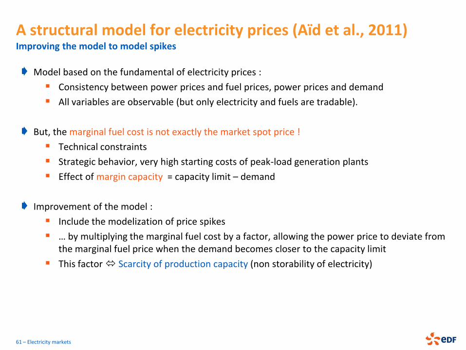
Model based on the fundamental of electricity prices :
Consistency between power prices and fuel prices, power prices and demand
All variables are observable (but only electricity and fuels are tradable).
But, the marginal fuel cost is not exactly the market spot price !
Technical constraints
Strategic behavior, very high starting costs of peak-load generation plants
Effect of margin capacity = capacity limit – demand
Improvement of the model :
Include the modelization of price spikes
… by multiplying the marginal fuel cost by a factor, allowing the power price to deviate from the marginal fuel price when the demand becomes closer to the capacity limit
This factor Scarcity of production capacity (non storability of electricity)
A structural model for electricity prices (Aïd et al., 2011) The model, improved to reproduce price spikes
62 – Electricity markets
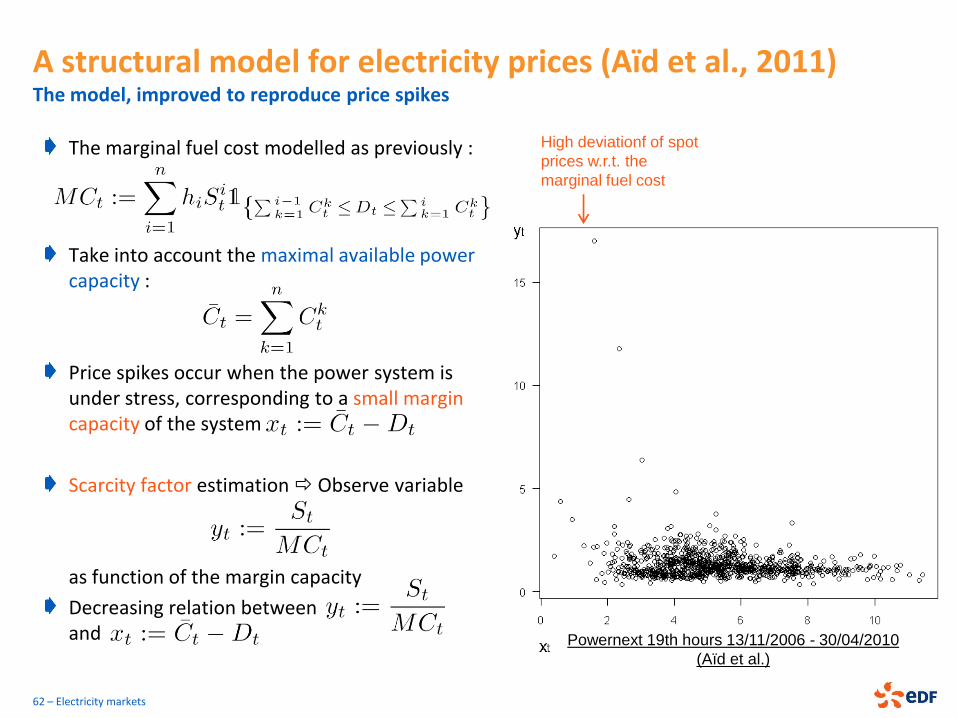
Powernext 19th hours 13/11/2006 - 30/04/2010
(Aïd et al.)
High deviationf of spot
prices w.r.t. the
marginal fuel cost
The marginal fuel cost modelled as previously :
Take into account the maximal available power capacity :
Price spikes occur when the power system is under stress, corresponding to a small margin capacity of the system
Scarcity factor estimation Observe variable
as function of the margin capacity
Decreasing relation between and
A structural model for electricity prices (Aïd et al., 2011) The model, improved to reproduce price spikes
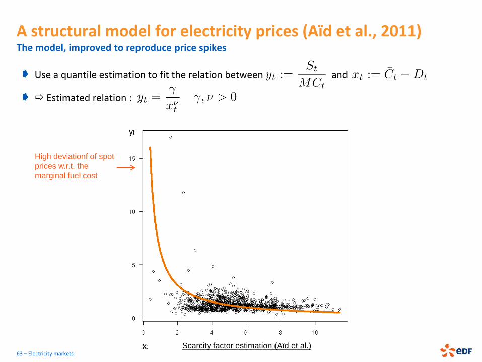
Use a quantile estimation to fit the relation between and
Estimated relation :
Scarcity factor estimation (Aïd et al.)
High deviationf of spot
prices w.r.t. the
marginal fuel cost
63 – Electricity markets
A structural model for electricity prices (Aïd et al., 2011) Backtesting the improved model
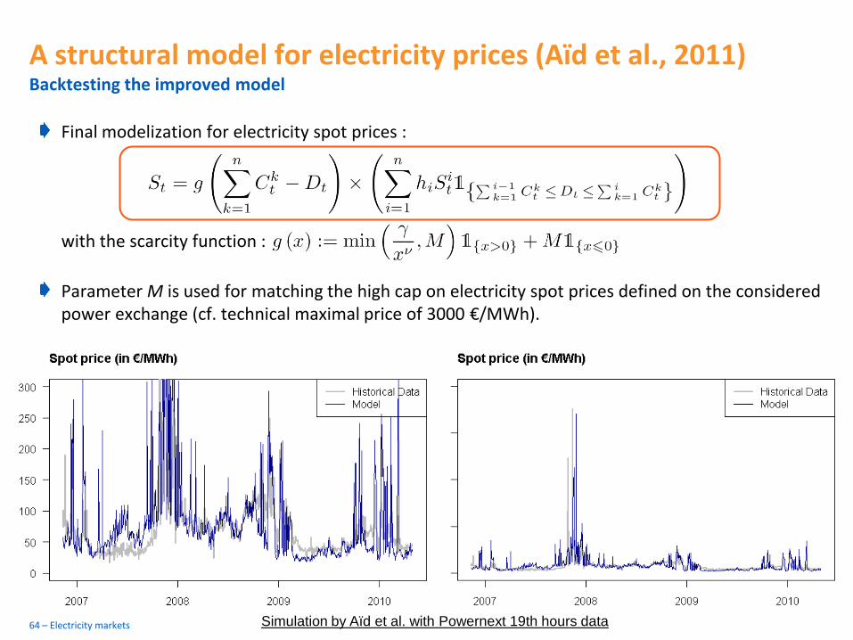
Final modelization for electricity spot prices :
with the scarcity function :
Parameter M is used for matching the high cap on electricity spot prices defined on the considered power exchange (cf. technical maximal price of 3000 €/MWh).
Simulation by Aïd et al. with Powernext 19th hours data 64 – Electricity markets
A structural model for electricity prices (Aïd et al., 2011) Pricing energy derivatives in this model
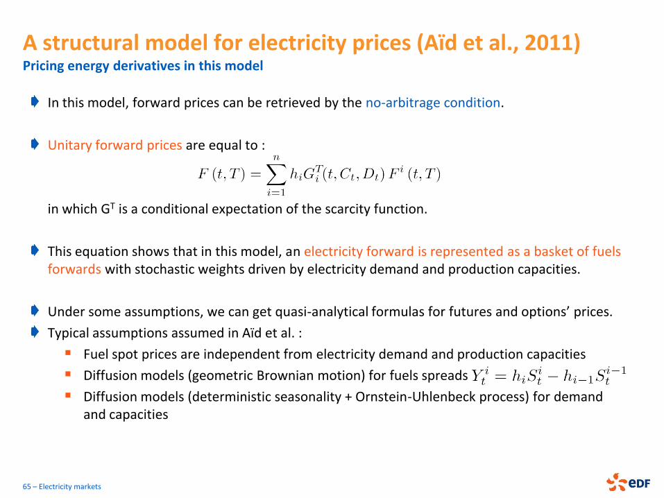
In this model, forward prices can be retrieved by the no-arbitrage condition.
Unitary forward prices are equal to :
in which GT is a conditional expectation of the scarcity function.
This equation shows that in this model, an electricity forward is represented as a basket of fuels forwards with stochastic weights driven by electricity demand and production capacities.
Under some assumptions, we can get quasi-analytical formulas for futures and options’ prices.
Typical assumptions assumed in Aïd et al. :
Fuel spot prices are independent from electricity demand and production capacities
Diffusion models (geometric Brownian motion) for fuels spreads
Diffusion models (deterministic seasonality + Ornstein-Uhlenbeck process) for demand and capacities
65 – Electricity markets
MODELLING ELECTRICITY PRICES
66 – Electricity markets
Main features of power forward prices
Overview of spot and forward models
A structural model for electricity prices (Aïd et al., 2011)
Factorial models for energy prices (e.g. Kiesel et al., 2008)
Forward curve modelling by factorial models Diffusion models for the forward curve
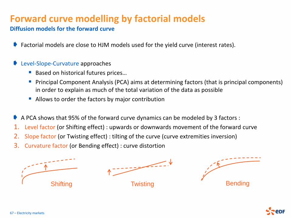
Factorial models are close to HJM models used for the yield curve (interest rates).
Level-Slope-Curvature approaches
Based on historical futures prices…
Principal Component Analysis (PCA) aims at determining factors (that is principal components) in order to explain as much of the total variation of the data as possible
Allows to order the factors by major contribution
A PCA shows that 95% of the forward curve dynamics can be modeled by 3 factors :
1. Level factor (or Shifting effect) : upwards or downwards movement of the forward curve
2. Slope factor (or Twisting effect) : tilting of the curve (curve extremities inversion)
3. Curvature factor (or Bending effect) : curve distortion
67 – Electricity markets
Shifting Twisting Bending
Forward curve modelling by factorial models Some basics on factorial models
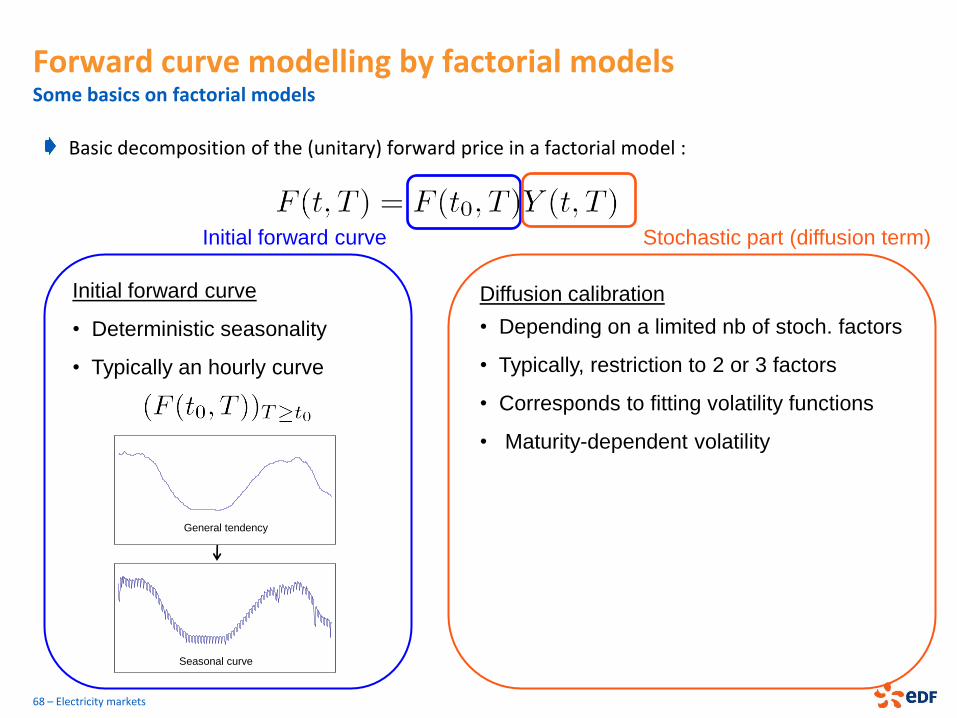
Basic decomposition of the (unitary) forward price in a factorial model :
68 – Electricity markets
Initial forward curve
• Deterministic seasonality
• Typically an hourly curve
General tendency
Seasonal curve
Diffusion calibration
• Depending on a limited nb of stoch. factors
• Typically, restriction to 2 or 3 factors
• Corresponds to fitting volatility functions
• Maturity-dependent volatility
Initial forward curve Stochastic part (diffusion term)

Diffusion
Delivery date
Forward prices
Random price
Price of 1MWh
delivered at time T
Quotation date
Initial price
Diffusion
Forward curve modelling by factorial models Notations : t0 = start of the diffusion, t = future observation date, T = start of delivery
69 – Electricity markets
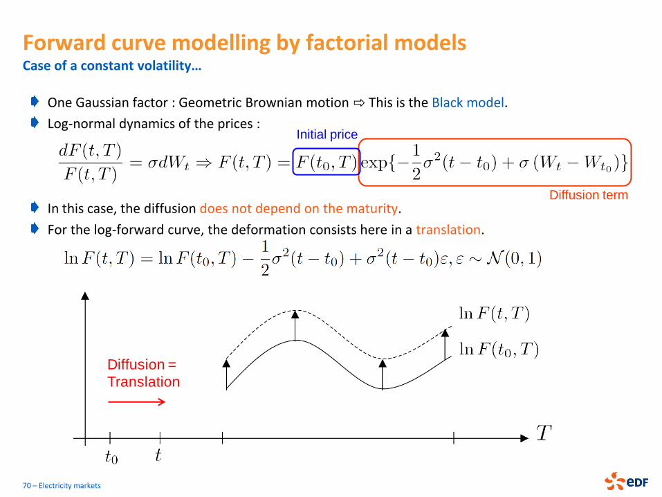
Forward curve modelling by factorial models Case of a constant volatility…
One Gaussian factor : Geometric Brownian motion ⇨ This is the Black model.
Log-normal dynamics of the prices :
In this case, the diffusion does not depend on the maturity.
For the log-forward curve, the deformation consists here in a translation.
70 – Electricity markets
Diffusion term
Initial price
Diffusion =
Translation
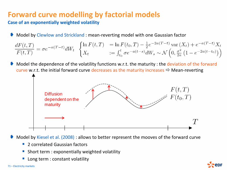
Forward curve modelling by factorial models Case of an exponentially weighted volatility
Model by Clewlow and Strickland : mean-reverting model with one Gaussian factor
Model the dependence of the volatility functions w.r.t. the maturity : the deviation of the forward curve w.r.t. the initial forward curve decreases as the maturity increases Mean-reverting
Model by Kiesel et al. (2008) : allows to better represent the mooves of the forward curve
2 correlated Gaussian factors
Short term : exponentially weighted volatility
Long term : constant volatility
71 – Electricity markets
Diffusion
dependent on the maturity
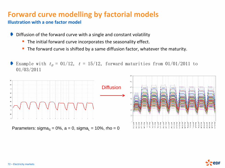
Diffusion of the forward curve with a single and constant volatility
The initial forward curve incorporates the seasonality effect.
The forward curve is shifted by a same diffusion factor, whatever the maturity.
Example with t0 = 01/12, t = 15/12, forward maturities from 01/01/2011 to 01/03/2011
72 – Electricity markets
Forward curve modelling by factorial models Illustration with a one factor model
Diffusion
Parameters: sigmaS = 0%, a = 0, sigmaL = 10%, rho = 0
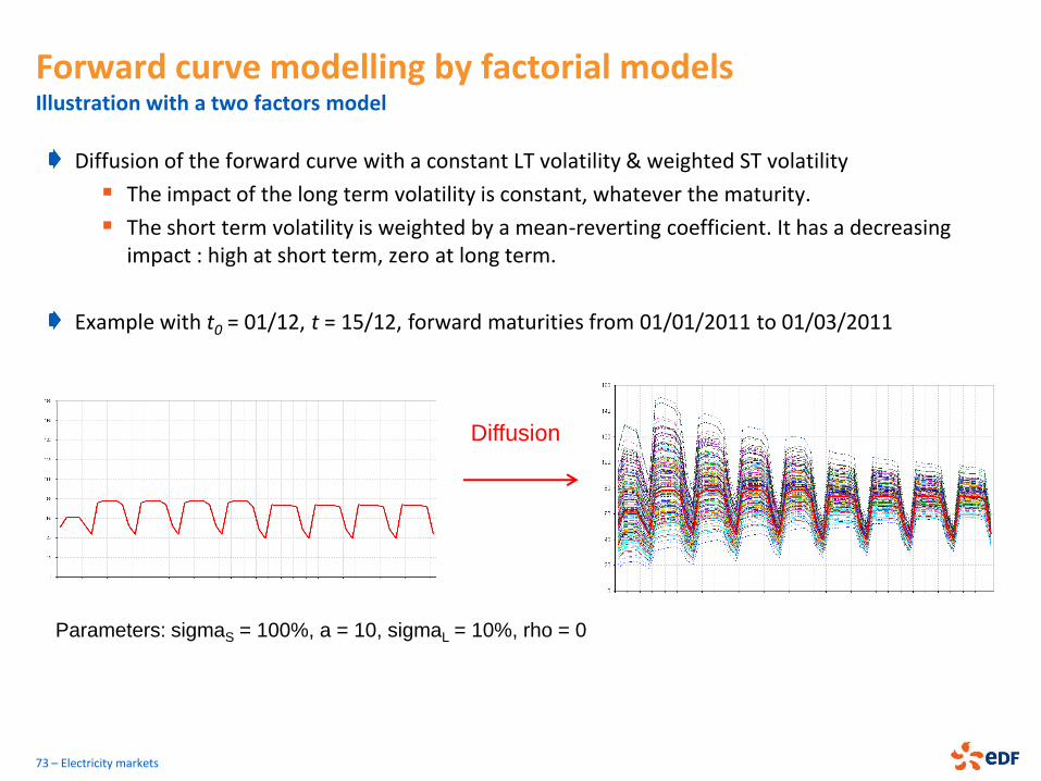
Diffusion of the forward curve with a constant LT volatility & weighted ST volatility
The impact of the long term volatility is constant, whatever the maturity.
The short term volatility is weighted by a mean-reverting coefficient. It has a decreasing impact : high at short term, zero at long term.
Example with t0 = 01/12, t = 15/12, forward maturities from 01/01/2011 to 01/03/2011
73 – Electricity markets
Forward curve modelling by factorial models Illustration with a two factors model
Diffusion
Parameters: sigmaS = 100%, a = 10, sigmaL = 10%, rho = 0