Electricity and Magnetism Energy of the Magnetic Field...

Electricity and MagnetismEnergy of the Magnetic Field

Mutual Inductance

Lana Sheridan

De Anza College

Mar 14, 2018

Last time

• inductors

• resistor-inductor circuits

Overview

• wrap up resistor-inductor circuits

• energy stored in an inductor

• coaxial inductor

• mutual inductance

Reminder: InductorsA capacitor is a device that stores an electric field as a componentof a circuit.

inductor

a device that stores a magnetic field in a circuit

It is typically a coil of wire.

Reminder: Inductance

inductance

the constant of proportionality relating the magnetic flux linkage(NΦB) to the current:

NΦB = L I ; L =NΦB

I

ΦB is the magnetic flux through the coil, and I is the current inthe coil.

RL Circuits: current rising

Current in loop:

974 Chapter 32 Inductance

After switch S1 is thrown closed at t ! 0, the current increases toward its maximum value e/R.

t !

L

t

R R0.632

i

e

t

Re

Figure 32.3 Plot of the current versus time for the RL circuit shown in Figure 32.2. The time constant t is the time interval required for i to reach 63.2% of its maximum value.

becomes zero and there is no time dependence of the current in this case; the cur-rent increases instantaneously to its final equilibrium value in the absence of the inductance. We can also write this expression as

i 5eR11 2 e2t/t 2 (32.7)

where the constant t is the time constant of the RL circuit:

t 5LR

(32.8)

Physically, t is the time interval required for the current in the circuit to reach (1 2 e21) 5 0.632 5 63.2% of its final value e/R. The time constant is a useful parameter for comparing the time responses of various circuits. Figure 32.3 shows a graph of the current versus time in the RL circuit. Notice that the equilibrium value of the current, which occurs as t approaches infinity, is e/R. That can be seen by setting di/dt equal to zero in Equation 32.6 and solving for the current i. (At equilibrium, the change in the current is zero.) Therefore, the current initially increases very rapidly and then gradually approaches the equilib-rium value e/R as t approaches infinity. Let’s also investigate the time rate of change of the current. Taking the first time derivative of Equation 32.7 gives

didt

5eL

e2 t/t (32.9)

This result shows that the time rate of change of the current is a maximum (equal to e/L) at t 5 0 and falls off exponentially to zero as t approaches infinity (Fig. 32.4). Now consider the RL circuit in Figure 32.2 again. Suppose switch S2 has been set at position a long enough (and switch S1 remains closed) to allow the current to reach its equilibrium value e/R. In this situation, the circuit is described by the outer loop in Figure 32.2. If S2 is thrown from a to b, the circuit is now described by only the right-hand loop in Figure 32.2. Therefore, the battery has been eliminated from the circuit. Setting e 5 0 in Equation 32.6 gives

iR 1 L didt

5 0

The time rate of change of current is a maximum at t ! 0, which is the instant at which switch S1 is thrown closed.

didt

t

Le

Figure 32.4 Plot of di/dt versus time for the RL circuit shown in Fig-ure 32.2. The rate decreases exponen-tially with time as i increases toward its maximum value.

i(t) =E

R

(1 − e−Rt/L

)

Derivative of current:


After switch S1 is thrown closed at t ! 0, the current increases toward its maximum value e/R.

t !

L

t

R R0.632

i

e

t

Re

Figure 32.3 Plot of the current versus time for the RL circuit shown in Figure 32.2. The time constant t is the time interval required for i to reach 63.2% of its maximum value.

becomes zero and there is no time dependence of the current in this case; the cur-rent increases instantaneously to its final equilibrium value in the absence of the inductance. We can also write this expression as

i 5eR11 2 e2t/t 2 (32.7)

where the constant t is the time constant of the RL circuit:

t 5LR

(32.8)

Physically, t is the time interval required for the current in the circuit to reach (1 2 e21) 5 0.632 5 63.2% of its final value e/R. The time constant is a useful parameter for comparing the time responses of various circuits. Figure 32.3 shows a graph of the current versus time in the RL circuit. Notice that the equilibrium value of the current, which occurs as t approaches infinity, is e/R. That can be seen by setting di/dt equal to zero in Equation 32.6 and solving for the current i. (At equilibrium, the change in the current is zero.) Therefore, the current initially increases very rapidly and then gradually approaches the equilib-rium value e/R as t approaches infinity. Let’s also investigate the time rate of change of the current. Taking the first time derivative of Equation 32.7 gives

didt

5eL

e2 t/t (32.9)

This result shows that the time rate of change of the current is a maximum (equal to e/L) at t 5 0 and falls off exponentially to zero as t approaches infinity (Fig. 32.4). Now consider the RL circuit in Figure 32.2 again. Suppose switch S2 has been set at position a long enough (and switch S1 remains closed) to allow the current to reach its equilibrium value e/R. In this situation, the circuit is described by the outer loop in Figure 32.2. If S2 is thrown from a to b, the circuit is now described by only the right-hand loop in Figure 32.2. Therefore, the battery has been eliminated from the circuit. Setting e 5 0 in Equation 32.6 gives

iR 1 L didt

5 0

The time rate of change of current is a maximum at t ! 0, which is the instant at which switch S1 is thrown closed.

didt

t

Le

Figure 32.4 Plot of di/dt versus time for the RL circuit shown in Fig-ure 32.2. The rate decreases exponen-tially with time as i increases toward its maximum value.

di

dt=

E

Le−Rt/L

RL Circuits: current rising

Potential drop across resistor:

80930-9 R L CI RCU ITSPART 3

VL (! L di/dt) across the inductor vary with time for particular values of !, L,and R. Compare this figure carefully with the corresponding figure for an RCcircuit (Fig. 27-16).

To show that the quantity tL (! L/R) has the dimension of time, we convertfrom henries per ohm as follows:

The first quantity in parentheses is a conversion factor based on Eq. 30-35, andthe second one is a conversion factor based on the relation V ! iR.

The physical significance of the time constant follows from Eq. 30-41. If weput t ! tL ! L/R in this equation, it reduces to

(30-43)

Thus, the time constant tL is the time it takes the current in the circuit to reachabout 63% of its final equilibrium value !/R. Since the potential difference VR

across the resistor is proportional to the current i, a graph of the increasingcurrent versus time has the same shape as that of VR in Fig. 30-17a.

If the switch S in Fig. 30-15 is closed on a long enough for the equilibriumcurrent !/R to be established and then is thrown to b, the effect will be to removethe battery from the circuit. (The connection to b must actually be made aninstant before the connection to a is broken. A switch that does this is called amake-before-break switch.) With the battery gone, the current through the resis-tor will decrease. However, it cannot drop immediately to zero but must decay tozero over time. The differential equation that governs the decay can be found byputting ! ! 0 in Eq. 30-39:

(30-44)

By analogy with Eqs. 27-38 and 27-39, the solution of this differential equationthat satisfies the initial condition i(0) ! i0 ! !/R is

(decay of current). (30-45)

We see that both current rise (Eq. 30-41) and current decay (Eq. 30-45) in an RLcircuit are governed by the same inductive time constant, tL.

We have used i0 in Eq. 30-45 to represent the current at time t ! 0. In ourcase that happened to be !/R, but it could be any other initial value.

i !!

R e"t/#L ! i0e"t/#L

L didt

$ iR ! 0.

i !!

R (1 " e"1) ! 0.63

!

R.

1 H%

! 1 H%

! 1 V & s1 H &A " ! 1 %&A

1 V " ! 1 s.

Fig. 30-17 The variation with time of(a) VR, the potential difference across theresistor in the circuit of Fig. 30-16, and (b)VL, the potential difference across the in-ductor in that circuit.The small trianglesrepresent successive intervals of one induc-tive time constant tL ! L/R.The figure isplotted for R ! 2000 %, L ! 4.0 H, and ! ! 10 V.

10 8 6 4 2

0 2 4 6 8

V R (

V)

t (ms)

0 2 4 6 8

V L (

V)

t (ms)

(a)

(b)

10 8 6 4 2

The resistor's potentialdifference turns on.The inductor's potentialdifference turns off.

CHECKPOINT 6

The figure shows three circuits with identical batteries, inductors, and resistors. Rankthe circuits according to the current through the battery (a) just after the switch isclosed and (b) a long time later, greatest first. (If you have trouble here, work throughthe next sample problem and then try again.)

(1) (2) (3)

halliday_c30_791-825hr.qxd 11-12-2009 12:19 Page 809

VR = iR

emf across inductor:

80930-9 R L CI RCU ITSPART 3

VL (! L di/dt) across the inductor vary with time for particular values of !, L,and R. Compare this figure carefully with the corresponding figure for an RCcircuit (Fig. 27-16).

To show that the quantity tL (! L/R) has the dimension of time, we convertfrom henries per ohm as follows:

The first quantity in parentheses is a conversion factor based on Eq. 30-35, andthe second one is a conversion factor based on the relation V ! iR.

The physical significance of the time constant follows from Eq. 30-41. If weput t ! tL ! L/R in this equation, it reduces to

(30-43)

Thus, the time constant tL is the time it takes the current in the circuit to reachabout 63% of its final equilibrium value !/R. Since the potential difference VR

across the resistor is proportional to the current i, a graph of the increasingcurrent versus time has the same shape as that of VR in Fig. 30-17a.

If the switch S in Fig. 30-15 is closed on a long enough for the equilibriumcurrent !/R to be established and then is thrown to b, the effect will be to removethe battery from the circuit. (The connection to b must actually be made aninstant before the connection to a is broken. A switch that does this is called amake-before-break switch.) With the battery gone, the current through the resis-tor will decrease. However, it cannot drop immediately to zero but must decay tozero over time. The differential equation that governs the decay can be found byputting ! ! 0 in Eq. 30-39:

(30-44)

By analogy with Eqs. 27-38 and 27-39, the solution of this differential equationthat satisfies the initial condition i(0) ! i0 ! !/R is

(decay of current). (30-45)

We see that both current rise (Eq. 30-41) and current decay (Eq. 30-45) in an RLcircuit are governed by the same inductive time constant, tL.

We have used i0 in Eq. 30-45 to represent the current at time t ! 0. In ourcase that happened to be !/R, but it could be any other initial value.

i !!

R e"t/#L ! i0e"t/#L

L didt

$ iR ! 0.

i !!

R (1 " e"1) ! 0.63

!

R.

1 H%

! 1 H%

! 1 V & s1 H &A " ! 1 %&A

1 V " ! 1 s.

Fig. 30-17 The variation with time of(a) VR, the potential difference across theresistor in the circuit of Fig. 30-16, and (b)VL, the potential difference across the in-ductor in that circuit.The small trianglesrepresent successive intervals of one induc-tive time constant tL ! L/R.The figure isplotted for R ! 2000 %, L ! 4.0 H, and ! ! 10 V.

10 8 6 4 2

0 2 4 6 8

V R (

V)

t (ms)

0 2 4 6 8

V L (

V)

t (ms)

(a)

(b)

10 8 6 4 2

The resistor's potentialdifference turns on.The inductor's potentialdifference turns off.

CHECKPOINT 6

The figure shows three circuits with identical batteries, inductors, and resistors. Rankthe circuits according to the current through the battery (a) just after the switch isclosed and (b) a long time later, greatest first. (If you have trouble here, work throughthe next sample problem and then try again.)

(1) (2) (3)


|EL(t)| = Ldi

dt

RL Circuits: Time Constant

τL = L/R

τL is called the time constant of the circuit.

(Notice that it is defined differently for RL circuits as opposed toRC circuits.)

This gives the time for the current to reach (1 − e−1) = 63.2% ofits final value.

Alternatively, it is the time for the potential drop across theinductor to fall to 1/e of its initial value.

It is useful for comparing the “relaxation time” of differentRL-circuits.

RL Circuits: current falling

80730-9 RL CI RCU ITSPART 3

This means that when a self-induced emf is produced in the inductor of Fig. 30-13,we cannot define an electric potential within the inductor itself, where the fluxis changing. However, potentials can still be defined at points of the circuit thatare not within the inductor—points where the electric fields are due to chargedistributions and their associated electric potentials.

Moreover, we can define a self-induced potential difference VL across aninductor (between its terminals, which we assume to be outside the region ofchanging flux). For an ideal inductor (its wire has negligible resistance), the mag-nitude of VL is equal to the magnitude of the self-induced emf !L.

If, instead, the wire in the inductor has resistance r, we mentally separate theinductor into a resistance r (which we take to be outside the region of changingflux) and an ideal inductor of self-induced emf !L. As with a real battery of emf! and internal resistance r, the potential difference across the terminals of a realinductor then differs from the emf. Unless otherwise indicated, we assume herethat inductors are ideal.

Fig. 30-14 (a) The current i is increasing,and the self-induced emf !L appears alongthe coil in a direction such that it opposesthe increase.The arrow representing !L canbe drawn along a turn of the coil or along-side the coil. Both are shown. (b) The cur-rent i is decreasing, and the self-induced emfappears in a direction such that it opposesthe decrease.

CHECKPOINT 5

The figure shows an emf !L induced in a coil. Which of the following can describe the current through the coil: (a)constant and rightward, (b) constant and leftward, (c) in-creasing and rightward, (d) decreasing and rightward,(e) increasing and leftward, (f) decreasing and leftward?

L

30-9 RL CircuitsIn Section 27-9 we saw that if we suddenly introduce an emf ! into a single-loopcircuit containing a resistor R and a capacitor C, the charge on the capacitor doesnot build up immediately to its final equilibrium value C! but approaches it in anexponential fashion:

(30-36)

The rate at which the charge builds up is determined by the capacitive timeconstant tC, defined in Eq. 27-36 as

tC ! RC. (30-37)

If we suddenly remove the emf from this same circuit, the charge does notimmediately fall to zero but approaches zero in an exponential fashion:

(30-38)

The time constant tC describes the fall of the charge as well as its rise.An analogous slowing of the rise (or fall) of the current occurs if we introduce

an emf ! into (or remove it from) a single-loop circuit containing a resistor R andan inductor L. When the switch S in Fig. 30-15 is closed on a, for example, the cur-rent in the resistor starts to rise. If the inductor were not present, the currentwould rise rapidly to a steady value !/R. Because of the inductor, however, a self-induced emf !L appears in the circuit; from Lenz’s law, this emf opposes the rise ofthe current, which means that it opposes the battery emf ! in polarity. Thus, thecurrent in the resistor responds to the difference between two emfs, a constant !due to the battery and a variable !L (! "L di/dt) due to self-induction.As long as!L is present, the current will be less than !/R.

As time goes on, the rate at which the current increases becomes less rapidand the magnitude of the self-induced emf, which is proportional to di/dt,becomes smaller. Thus, the current in the circuit approaches !/R asymptotically.

q ! q0e"t/#C.

q ! C!(1 " e"t/#C).

i (increasing)

(a)

i (decreasing)

(b)

L

L

L

L

The changing current changes the flux, whichcreates an emf that opposes the change.

Fig. 30-15 An RL circuit.When switchS is closed on a, the current rises and ap-proaches a limiting value !/R.

Sa

b R

L–+


Battery switched out - switch to b.Loop rule:

−EL − iR = 0

−Ldi

dt−iR = 0

Solution:

i =E

Re−t/τL ; τL =

L

R

RL Circuits: current falling

32.2 RL Circuits 975

Example 32.2 Time Constant of an RL Circuit

Consider the circuit in Figure 32.2 again. Suppose the circuit elements have the following values: e 5 12.0 V, R 5 6.00 V, and L 5 30.0 mH.

(A) Find the time constant of the circuit.

Conceptualize You should understand the operation and behavior of the circuit in Figure 32.2 from the discussion in this section.

Categorize We evaluate the results using equations developed in this section, so this example is a substitution problem.

S O L U T I O N

Evaluate the time constant from Equation 32.8: t 5LR

530.0 3 1023 H

6.00 V5 5.00 ms

(B) Switch S2 is at position a, and switch S1 is thrown closed at t 5 0. Calculate the current in the circuit at t 5 2.00 ms.

S O L U T I O N

Evaluate the current at t 5 2.00 ms from Equation 32.7:

i 5eR

11 2 e2t/t 2 512.0 V6.00 V

11 2 e22.00 ms/5.00 ms 2 5 2.00 A 11 2 e20.400 25 0.659 A

(C) Compare the potential difference across the resistor with that across the inductor.

At the instant the switch is closed, there is no current and therefore no potential difference across the resistor. At this instant, the battery voltage appears entirely across the inductor in the form of a back emf of 12.0 V as the inductor tries to maintain the zero-current condition. (The top end of the inductor in Fig. 32.2 is at a higher electric potential than the bottom end.) As time passes, the emf across the inductor decreases and the current in the resistor (and hence the voltage across it) increases as shown in Figure 32.6 (page 976). The sum of the two voltages at all times is 12.0 V.

In Figure 32.6, the voltages across the resistor and inductor are equal at 3.4 ms. What if you wanted to delay the condition in which the voltages are equal to some later instant, such as t 5 10.0 ms? Which parameter, L or R, would require the least adjustment, in terms of a percentage change, to achieve that?

S O L U T I O N

WHAT IF ?

At t ! 0, the switch is thrown to position b and the current has its maximum value e/R.

i

t

Re

Figure 32.5 Current versus time for the right-hand loop of the circuit shown in Figure 32.2. For t , 0, switch S2 is at position a.

It is left as a problem (Problem 22) to show that the solution of this differential equation is

i 5eR

e2t/t 5 Ii e2t/t (32.10)

where e is the emf of the battery and Ii 5 e/R is the initial current at the instant the switch is thrown to b. If the circuit did not contain an inductor, the current would immediately decrease to zero when the battery is removed. When the inductor is present, it opposes the decrease in the current and causes the current to decrease exponen-tially. A graph of the current in the circuit versus time (Fig. 32.5) shows that the current is continuously decreasing with time.

Q uick Quiz 32.2 Consider the circuit in Figure 32.2 with S1 open and S2 at posi-tion a. Switch S1 is now thrown closed. (i) At the instant it is closed, across which circuit element is the voltage equal to the emf of the battery? (a) the resistor (b) the inductor (c) both the inductor and resistor (ii) After a very long time, across which circuit element is the voltage equal to the emf of the battery? Choose from among the same answers.

continued

i =E

Re−t/τL ; τL =

L

R

Energy Stored in a Magnetic Field in an Inductor

Power delivered to inductor:

P = I |EL|

Energy stored in inductor carrying current i :

UB =

∫P dt =

∫ i0i ′(L

di′

dt

)dt

UB =1

2Li2

Compare with UE = Q2

2C (or UE = 12CV

2) for the energy stored in acapacitor.

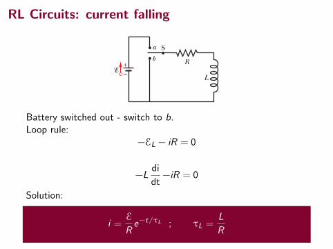
Energy Density of a Magnetic Field

The energy density of a magnetic field is the energy stored perunit volume.

uB =UB

A`

where A is the cross-sectional area of a solenoid and ` is thelength.

uB =L

A`

i2

2

Remember, L = µ0n2A` and B = µ0in.

Energy Density of a Magnetic Field

uB =B2

2µ0

Compare with uE = 12ε0E

2 for electric fields.

Energy Density of a Magnetic Field Question

Which of the following adjustments increases the energy density ina solenoid?

(A) increasing the number of turns per unit length on the solenoid

(B) increasing the cross-sectional area of the solenoid

(C) increasing the current in the solenoid

(D) two of the above

Energy Density of a Magnetic Field Question

Which of the following adjustments increases the energy density ina solenoid?

(A) increasing the number of turns per unit length on the solenoid

(B) increasing the cross-sectional area of the solenoid

(C) increasing the current in the solenoid

(D) two of the above←

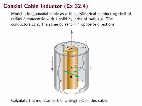
Coaxial Cable Inductor (Ex 32.4)Model a long coaxial cable as a thin, cylindrical conducting shell ofradius b concentric with a solid cylinder of radius a. Theconductors carry the same current i in opposite directions.


Use Equation 32.2 to find the inductance of the cable: L 5FB

i5

m0,

2p ln a b

abSubstitute for the magnetic field and integrate over the entire light gold rectangle:

FB 5 3b

a m0 i2pr

, dr 5m0 i,

2p 3

b

a drr

5m0 i,

2p ln a b

a b

Divide the light gold rectangle into strips of width dr such as the darker strip in Figure 32.7. Evaluate the mag-netic flux through such a strip:

dFB 5 B dA 5 B, dr

Finalize The inductance depends only on geometric factors related to the cable. It increases if , increases, if b increases, or if a decreases. This result is consistent with our conceptualization: any of these changes increases the size of the loop represented by our radial slice and through which the magnetic field passes, increasing the inductance.

32.4 Mutual InductanceVery often, the magnetic flux through the area enclosed by a circuit varies with time because of time-varying currents in nearby circuits. This condition induces an

Example 32.4 The Coaxial Cable

Coaxial cables are often used to connect electrical devices, such as your video system, and in receiving signals in television cable systems. Model a long coaxial cable as a thin, cylindrical conducting shell of radius b concentric with a solid cylinder of radius a as in Figure 32.7. The conductors carry the same current I in opposite directions. Calculate the inductance L of a length , of this cable.

Conceptualize Consider Figure 32.7. Although we do not have a visible coil in this geometry, imagine a thin, radial slice of the coaxial cable such as the light gold rectangle in Figure 32.7. If the inner and outer conductors are connected at the ends of the cable (above and below the figure), this slice represents one large conducting loop. The current in the loop sets up a magnetic field between the inner and outer conductors that passes through this loop. If the current changes, the magnetic field changes and the induced emf opposes the original change in the current in the conductors.

Categorize We categorize this situation as one in which we must return to the fundamental definition of inductance, Equation 32.2.

Analyze We must find the magnetic flux through the light gold rectangle in Figure 32.7. Ampère’s law (see Section 30.3) tells us that the magnetic field in the region between the conductors is due to the inner conductor alone and that its magnitude is B 5 m0i/2pr, where r is measured from the common center of the cylinders. A sample circular field line is shown in Figure 32.7, along with a field vector tangent to the field line. The magnetic field is zero outside the outer shell because the net current passing through the area enclosed by a circular path surrounding the cable is zero; hence, from Ampère’s law, r B

S ? d sS 5 0.

The magnetic field is perpendicular to the light gold rectangle of length , and width b 2 a, the cross section of interest. Because the magnetic field varies with radial position across this rectangle, we must use calculus to find the total magnetic flux.

S O L U T I O N

i

!

bdr

ri

a

BS

Figure 32.7 (Example 32.4) Sec-tion of a long coaxial cable. The inner and outer conductors carry equal cur-rents in opposite directions.

▸ 32.3 c o n t i n u e d

Finalize This result is equal to the initial energy stored in the magnetic field of the inductor, given by Equation 32.12, as we set out to prove.

Calculate the inductance L of a length `, of this cable.

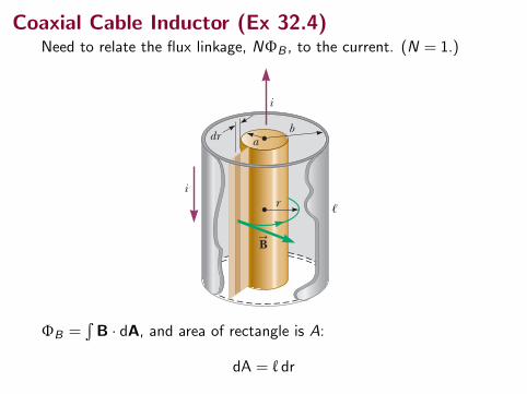
Coaxial Cable Inductor (Ex 32.4)Need to relate the flux linkage, NΦB , to the current. (N = 1.)


Use Equation 32.2 to find the inductance of the cable: L 5FB

i5

m0,

2p ln a b

abSubstitute for the magnetic field and integrate over the entire light gold rectangle:

FB 5 3b

a m0 i2pr

, dr 5m0 i,

2p 3

b

a drr

5m0 i,

2p ln a b

a b

Divide the light gold rectangle into strips of width dr such as the darker strip in Figure 32.7. Evaluate the mag-netic flux through such a strip:

dFB 5 B dA 5 B, dr

Finalize The inductance depends only on geometric factors related to the cable. It increases if , increases, if b increases, or if a decreases. This result is consistent with our conceptualization: any of these changes increases the size of the loop represented by our radial slice and through which the magnetic field passes, increasing the inductance.

32.4 Mutual InductanceVery often, the magnetic flux through the area enclosed by a circuit varies with time because of time-varying currents in nearby circuits. This condition induces an

Example 32.4 The Coaxial Cable

Coaxial cables are often used to connect electrical devices, such as your video system, and in receiving signals in television cable systems. Model a long coaxial cable as a thin, cylindrical conducting shell of radius b concentric with a solid cylinder of radius a as in Figure 32.7. The conductors carry the same current I in opposite directions. Calculate the inductance L of a length , of this cable.

Conceptualize Consider Figure 32.7. Although we do not have a visible coil in this geometry, imagine a thin, radial slice of the coaxial cable such as the light gold rectangle in Figure 32.7. If the inner and outer conductors are connected at the ends of the cable (above and below the figure), this slice represents one large conducting loop. The current in the loop sets up a magnetic field between the inner and outer conductors that passes through this loop. If the current changes, the magnetic field changes and the induced emf opposes the original change in the current in the conductors.

Categorize We categorize this situation as one in which we must return to the fundamental definition of inductance, Equation 32.2.

Analyze We must find the magnetic flux through the light gold rectangle in Figure 32.7. Ampère’s law (see Section 30.3) tells us that the magnetic field in the region between the conductors is due to the inner conductor alone and that its magnitude is B 5 m0i/2pr, where r is measured from the common center of the cylinders. A sample circular field line is shown in Figure 32.7, along with a field vector tangent to the field line. The magnetic field is zero outside the outer shell because the net current passing through the area enclosed by a circular path surrounding the cable is zero; hence, from Ampère’s law, r B

S ? d sS 5 0.

The magnetic field is perpendicular to the light gold rectangle of length , and width b 2 a, the cross section of interest. Because the magnetic field varies with radial position across this rectangle, we must use calculus to find the total magnetic flux.

S O L U T I O N

i

!

bdr

ri

a

BS

Figure 32.7 (Example 32.4) Sec-tion of a long coaxial cable. The inner and outer conductors carry equal cur-rents in opposite directions.

▸ 32.3 c o n t i n u e d

Finalize This result is equal to the initial energy stored in the magnetic field of the inductor, given by Equation 32.12, as we set out to prove.

ΦB =∫B · dA, and area of rectangle is A:

dA = ` dr

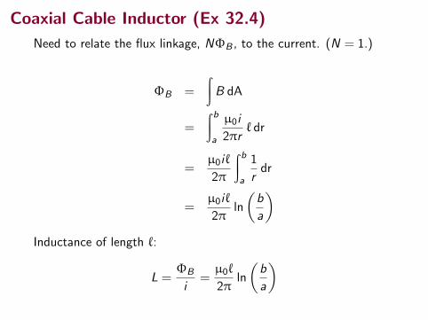
Coaxial Cable Inductor (Ex 32.4)

Need to relate the flux linkage, NΦB , to the current. (N = 1.)

ΦB =

∫B dA

=

∫ba

µ0i

2πr` dr

=µ0i`

2π

∫ba

1

rdr

=µ0i`

2πln

(b

a

)

Inductance of length `:

L =ΦB

i=µ0`

2πln

(b

a

)

Coaxial Cable Inductor (Ex 32.4)

Need to relate the flux linkage, NΦB , to the current. (N = 1.)

ΦB =

∫B dA

=

∫ba

µ0i

2πr` dr

=µ0i`

2π

∫ba

1

rdr

=µ0i`

2πln

(b

a

)Inductance of length `:

L =ΦB

i=µ0`

2πln

(b

a

)

Mutual Inductance

An inductor can have an induced emf from its own changingmagnetic field.

It also can have an emf from an external changing field.

That external changing field could be another inductor.

For self-inductance on a coil labeled 1:

N1ΦB,1 = L1i1

For mutual inductance:

N1ΦB,2→1 = M21i2

The flux is in coil 1, but the current that causes the flux is in coil 2.

Mutual InductanceFor mutual inductance:

N1ΦB,2→1 = M21i2

The flux is in coil 1, but the current that causes the flux is in coil 2.

which has the same form as Eq. 30-28,

L ! N"/i, (30-58)

the definition of inductance.We can recast Eq. 30-57 as

M21i1 ! N2"21. (30-59)

If we cause i1 to vary with time by varying R, we have

(30-60)

The right side of this equation is, according to Faraday’s law, just the magnitudeof the emf !2 appearing in coil 2 due to the changing current in coil 1.Thus, with aminus sign to indicate direction,

(30-61)

which you should compare with Eq. 30-35 for self-induction (! ! #L di/dt).Let us now interchange the roles of coils 1 and 2,as in Fig.30-19b; that is,we set up a

current i2 in coil 2 by means of a battery,and this produces a magnetic flux "12 that linkscoil 1.If we change i2 with time by varying R,we then have,by the argument given above,

(30-62)

Thus, we see that the emf induced in either coil is proportional to the rate ofchange of current in the other coil.The proportionality constants M21 and M12 seem tobe different. We assert, without proof, that they are in fact the same so that no sub-scripts are needed.(This conclusion is true but is in no way obvious.) Thus,we have

M21 ! M12 ! M, (30-63)

and we can rewrite Eqs. 30-61 and 30-62 as

(30-64)

and (30-65)!1 ! #M di2

dt.

!2 ! #M di1

dt

!1 ! #M12 di2

dt.

!2 ! #M21 di1

dt,

M21 di1

dt! N2

d"21

dt.

814 CHAPTE R 30 I N DUCTION AN D I N DUCTANCE

Fig. 30-19 Mutual induction. (a) Themagnetic field produced by current i1 incoil 1 extends through coil 2. If i1 is varied(by varying resistance R), an emf is inducedin coil 2 and current registers on the meterconnected to coil 2. (b) The roles of thecoils interchanged.

B:

1

+ –

i 1

N 1

Coil 1 Coil 2

B1

N 2 21 Φ

(a)

+ –

i 2

N 2

Coil 1 Coil 2(b)

N 1 12Φ

B2

B2

B1

R R

0 0


Mutual Inductance

mutual inductance

M =N1ΦB,2→1

i2=

N2ΦB,1→2

i1

which has the same form as Eq. 30-28,

L ! N"/i, (30-58)

the definition of inductance.We can recast Eq. 30-57 as

M21i1 ! N2"21. (30-59)

If we cause i1 to vary with time by varying R, we have

(30-60)

The right side of this equation is, according to Faraday’s law, just the magnitudeof the emf !2 appearing in coil 2 due to the changing current in coil 1.Thus, with aminus sign to indicate direction,

(30-61)

which you should compare with Eq. 30-35 for self-induction (! ! #L di/dt).Let us now interchange the roles of coils 1 and 2,as in Fig.30-19b; that is,we set up a

current i2 in coil 2 by means of a battery,and this produces a magnetic flux "12 that linkscoil 1.If we change i2 with time by varying R,we then have,by the argument given above,

(30-62)

Thus, we see that the emf induced in either coil is proportional to the rate ofchange of current in the other coil.The proportionality constants M21 and M12 seem tobe different. We assert, without proof, that they are in fact the same so that no sub-scripts are needed.(This conclusion is true but is in no way obvious.) Thus,we have

M21 ! M12 ! M, (30-63)

and we can rewrite Eqs. 30-61 and 30-62 as

(30-64)

and (30-65)!1 ! #M di2

dt.

!2 ! #M di1

dt

!1 ! #M12 di2

dt.

!2 ! #M21 di1

dt,

M21 di1

dt! N2

d"21

dt.

814 CHAPTE R 30 I N DUCTION AN D I N DUCTANCE

Fig. 30-19 Mutual induction. (a) Themagnetic field produced by current i1 incoil 1 extends through coil 2. If i1 is varied(by varying resistance R), an emf is inducedin coil 2 and current registers on the meterconnected to coil 2. (b) The roles of thecoils interchanged.

B:

1

+ –

i 1

N 1

Coil 1 Coil 2

B1

N 2 21 Φ

(a)

+ –

i 2

N 2

Coil 1 Coil 2(b)

N 1 12Φ

B2

B2

B1

R R

0 0


Mutual Inductance

N1ΦB,2→1 = M21i2

Considering the rate of change of both sides with time, and usingFaraday’s Law E = − dΦB

dt ,

E1 = −Mdi2dt

and

E2 = −Mdi1dt

A change of current in one coil causes a magnetic flux in the other.

Summary

• energy stored in the magnetic field

• coaxial inductor

• mutual inductance

• applications of mutual inductance

4th Collected Homework due Thursday Mar 22.

Quiz this Friday.

HomeworkSerway & Jewett:

• Ch 32, onward from page 988. Obj. Qs: 1; Conc. Qs.: 7;Probs: 11, 15, 19, 33, 41, 43

Electricity and Magnetism Energy of the Magnetic Field...

Documents

Transcript of Electricity and Magnetism Energy of the Magnetic Field...