Electrical Resonances and Harmonics in a Wind …lib.tkk.fi/Dipl/2012/urn100577.pdf · Aalto...
90
Aalto University School of Electrical Engineering Kalle Rauma Electrical Resonances and Harmonics in a Wind Power Plant Thesis submitted for examination for the degree of Master of Science in Technology Espoo, Finland 17 th February 2012 Supervisor: Prof. Liisa Haarla Instructor: D.Sc. (Tech.) Pedro Rodríguez
Transcript of Electrical Resonances and Harmonics in a Wind …lib.tkk.fi/Dipl/2012/urn100577.pdf · Aalto...
Aalto University School of Electrical Engineering Kalle Rauma
Electrical Resonances and Harmonics in a Wind Power Plant
Thesis submitted for examination for the degree of Master of Science in Technology Espoo, Finland 17th February 2012 Supervisor: Prof. Liisa Haarla Instructor: D.Sc. (Tech.) Pedro Rodríguez

AALTO UNIVERSITY SCHOOL OF ELECTRICAL ENGINEERING ABSTRACT Aalto University
School of Electrical Engineering
Author: Kalle Rauma
Name of the thesis: Electrical Resonances and Harmonics in a Wind Power Plant
Date: 17th February 2012 Number of pages: [9+81]
Supervisor: Prof. Liisa Haarla, Aalto University
Instructor: D.Sc. (Tech.) Pedro Rodríguez, Renewable Electrical Energy Systems,
Technical University of Catalonia
Language: English
Modern power networks have a growing number of power electronic devices, some of which can be seen as sources of harmonic currents. Moreover, the electric grids have numerous inductive and capacitive elements forming ideal conditions for harmonic resonances. These resonances, however, are a severe threat to power quality and the function of power systems. For this reason, the resonance analysis is an emerging topic in the field of power systems. In the current study, two analytical methods are used: a frequency scan and harmonic resonance mode analysis. Although the former method is well-known, the latter method is relatively new. The mathematical bases of these two methods are introduced in the theoretical section and then applied in the simulations of an aggregated model of an off shore wind power plant. The work has two principal objectives: to determine the main reasons for harmonic resonances in a wind power plant and to investigate the applicability of the harmonic resonance mode analysis to analyse the resonances. In addition to establishing the resonating elements in a wind power plant, the results reveal the harmonic resonance mode analysis to be a plausible tool for the systematic resonance analysis of power networks. The thesis offers new aspects of developing the modal approach to the resonance studies are provided. Keywords: resonance, wind power plant, harmonic resonance mode analysis, modal
analysis, harmonics, power quality
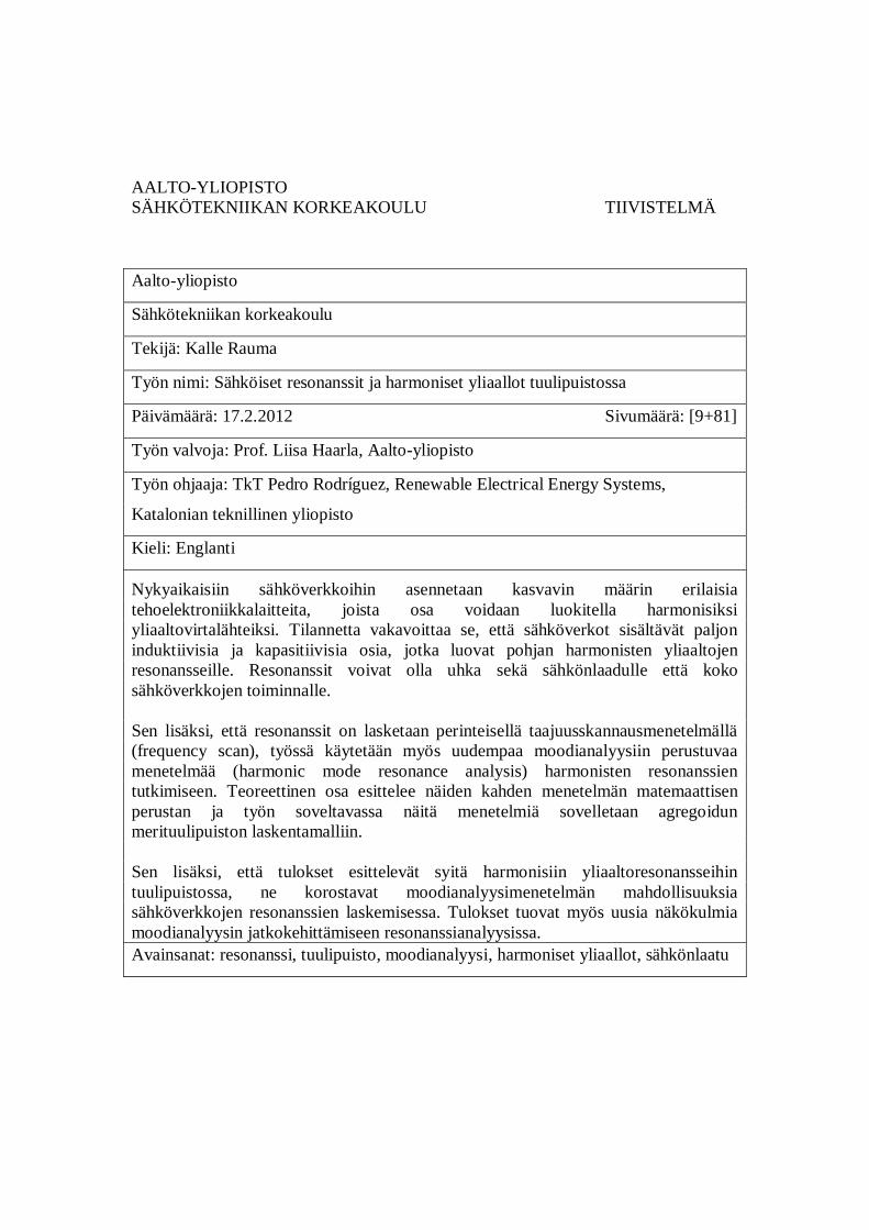
AALTO-YLIOPISTO SÄHKÖTEKNIIKAN KORKEAKOULU TIIVISTELMÄ Aalto-yliopisto
Sähkötekniikan korkeakoulu
Tekijä: Kalle Rauma
Työn nimi: Sähköiset resonanssit ja harmoniset yliaallot tuulipuistossa
Päivämäärä: 17.2.2012 Sivumäärä: [9+81]
Työn valvoja: Prof. Liisa Haarla, Aalto-yliopisto
Työn ohjaaja: TkT Pedro Rodríguez, Renewable Electrical Energy Systems,
Katalonian teknillinen yliopisto
Kieli: Englanti
Nykyaikaisiin sähköverkkoihin asennetaan kasvavin määrin erilaisia tehoelektroniikkalaitteita, joista osa voidaan luokitella harmonisiksi yliaaltovirtalähteiksi. Tilannetta vakavoittaa se, että sähköverkot sisältävät paljon induktiivisia ja kapasitiivisia osia, jotka luovat pohjan harmonisten yliaaltojen resonansseille. Resonanssit voivat olla uhka sekä sähkönlaadulle että koko sähköverkkojen toiminnalle. Sen lisäksi, että resonanssit on lasketaan perinteisellä taajuusskannausmenetelmällä (frequency scan), työssä käytetään myös uudempaa moodianalyysiin perustuvaa menetelmää (harmonic mode resonance analysis) harmonisten resonanssien tutkimiseen. Teoreettinen osa esittelee näiden kahden menetelmän matemaattisen perustan ja työn soveltavassa näitä menetelmiä sovelletaan agregoidun merituulipuiston laskentamalliin. Sen lisäksi, että tulokset esittelevät syitä harmonisiin yliaaltoresonansseihin tuulipuistossa, ne korostavat moodianalyysimenetelmän mahdollisuuksia sähköverkkojen resonanssien laskemisessa. Tulokset tuovat myös uusia näkökulmia moodianalyysin jatkokehittämiseen resonanssianalyysissa. Avainsanat: resonanssi, tuulipuisto, moodianalyysi, harmoniset yliaallot, sähkönlaatu

UNIVERSIDAD AALTO ESCUELA DE INGENIERÍA ELÉCTRICA RESUMEN Universidad Aalto
Escuela de Ingeniería Eléctrica
Autor: Kalle Rauma
Título de la tesis: Resonancias eléctricas y armónicos en un parque eólico
Fecha: 17 de febrero de 2012 Número de páginas: [9+81]
Supervisora: Prof. Liisa Haarla, Universidad Aalto
Instructor: Dr. Pedro Rodríguez, Sistemas Eléctricos de Energía Renovable,
Universitat Politècnica de Catalunya
Idioma: Inglés
Hoy en día se instalan una gran cantidad de aparatos de electrónica de potencia en las redes eléctricas y algunos de estos aparatos se consideran como fuentes de armónicos. Además, las redes eléctricas tienen varios componentes inductivos y capacitivos que juntos forman un entorno ideal para las resonancias armónicas. Las resonancias conforman una amenaza para la función de las redes eléctricas y para la calidad de suministro y por eso el análisis de las resonancias es un tópico emergente en el ámbito de las redes eléctricas. Además de calcular las resonancias con el escaneo de frecuencias se presenta un método relativamente reciente llamado análisis modal de las resonancias armónicas. La parte teórica introduce los fondos matemáticos de los dos métodos y la parte de las simulaciones aplica estos métodos en un modelo agregado de un parque eólico marino. El trabajo tiene dos objetivos principales: encontrar las razones de las resonancias armónicas en un parque eólico e investigar la aplicabilidad del método de análisis modal para analizar dichas resonancias. Los resultados no solamente describen las principales fuentes de las resonancias sino además matizan la importancia del método de análisis modal como una herramienta adicional para analizar las resonancias en redes eléctricas. Por otra parte se ofrecen nuevos aspectos de aplicación del análisis modal para estudiar las resonancias eléctricas. Palabras claves: resonancia, parque eólico, análisis modal, armónicos, calidad de
suministro

v
Acknowledgments
This Master´s thesis has been carried out at the research group of Renewable
Electrical Energy Systems in the Technical University of Catalonia (UPC) located in
the city of Terrassa in Spain.
Firstly, I would like to thank Alvaro Luna, since he gave me the possibility to be a
part of this great research group. I want to express my gratitude to my instructor Pedro
Rodríguez for his encourage and fresh ideas that made the work possible. In addition,
special acknowledgement goes to my supervisor Liisa Haarla, who is absolutely one
of the greatest professionals and certainly the most responsible professor that I have
met during my studies.
Special thanks to Khairul Nisak for her patience for working with me and Ignacio
Candela for his professional advice. It was always a joy to work with them.
Furthermore, I want to thank all the rest of the people from Renewable Electrical
Energy with whom I had great time inside and outside the university. I am glad
having the opportunity to be a member of one of the most competitive research groups
in the field of renewable energies in Spain. Even though the way of working of this
group was very productive, the work ambient was laid-back and, literally, warm and
sunny.
My stay in Spain would not have been easy or even likely without the support of
Xenia. In addition, I want to thank Lola and Mario for their great hospitality and all
the other people who have made my Mediterranean experience unforgettable.
Especially, I want to thank my family for supporting me in my studies during all these
years.
Terrassa, 11th November 2011
Kalle Rauma

vi
Acknowledgments .................................................................................. v
1 The Basics of Harmonic Analysis ................................................... 1
1.1 The Definition and Mathematical Form of Harmonics ............................................ 1
1.2 Generation of Harmonics .......................................................................................... 2
1.3 Indices Related to Harmonics ................................................................................... 2
1.4 Symmetrical Components Related to Harmonics .................................................... 3
1.5 Resonance Phenomena .............................................................................................. 4 1.5.1 Parallel Resonance ....................................................................................................... 4 1.5.2 Series Resonance ......................................................................................................... 5
2 Harmonics in a Wind Power Plant ................................................. 5
2.1 Importance of Resonance Analysis of a Wind Power Plant ..................................... 5
2.2 Direct Harm Caused by Harmonics ......................................................................... 6
2.3 Harmonic Sources in a Wind Power Plant ............................................................... 6 2.3.1 Power Converters in Wind Turbines ............................................................................. 7 2.3.2 Voltage Source Converter High Voltage Direct Current Links ...................................... 8 2.3.3 Flexible Alternative Current Transmission System Devices .......................................... 8
2.4 Increasing the Possibility of Harmonic Resonances ............................................... 10 2.4.1 Cable Connections ..................................................................................................... 10 2.4.2 Capacitor Banks and Reactors .................................................................................... 11
2.5 Harmonics Mitigation in a Wind Power Plant ....................................................... 11 2.5.1 Preventive Manners ................................................................................................... 11 2.5.2 Harmonic Filters ........................................................................................................ 12
2.5.2.1 Passive Filters ................................................................................................... 12 2.5.2.2 Active Filters .................................................................................................... 13 2.5.2.3 Hybrid Filters ................................................................................................... 13
2.6 Limits of German Electricity Association for Harmonic Currents ....................... 14
3 Computation Technique of Harmonic Analysis .......................... 15
3.1 Frequency Scan ....................................................................................................... 16
3.2 Harmonic Resonance Mode Analysis ..................................................................... 17 3.2.1 Sensitivity Matrix ...................................................................................................... 18 3.2.2 Eigenvalue Sensitivities with Respect to Power System Components .......................... 19 3.2.3 The Connection between Modes and Impedances of the Frequency Scan .................... 20
4 Simulations – Aggregated Wind Power Plant ............................. 20
4.1 Modelling the Wind Power Plant ............................................................................ 21
4.2 Resonance Analysis of the Wind Power Plant ........................................................ 24
4.3 The Effect of the Collector Cable Length on the Resonance Points....................... 29
4.4 The Effect of Transmission Cable Length on the Resonance Points...................... 37
4.5 Passive Filters at the Critical Buses ........................................................................ 39
4.6 Hybrid Filters at the Critical Buses ........................................................................ 43
4.7 Harmonic Current and Voltage Analyses............................................................... 48 4.7.1 Harmonic Current and Voltage Analysis of the Wind Power Plant .............................. 48 4.7.2 Harmonic Current and Voltage Analysis with Passive Filters ...................................... 55
4.8 The Impact of Skin Effect on Modal Analysis ........................................................ 59

vii
5 Analysis of the Results .................................................................. 62
5.1 Resonance Analysis of the Wind Power Plant ........................................................ 62
5.2 The Effect of Collector and Transmission Cable Lengths on Resonance Points ... 63
5.3 Adding Filters at Critical Buses .............................................................................. 64
5.4 Harmonic Current and Voltage Analyses............................................................... 65
5.5 Impact of the Skin Effect on Modal Analysis ......................................................... 67
6 Discussion ...................................................................................... 67
7 Conclusions and Future Work ..................................................... 68
7.1 Conclusions .............................................................................................................. 68
7.2 Future Work ............................................................................................................ 68
References ............................................................................................ 70
Appendix A........................................................................................... 78
Appendix B ........................................................................................... 80

viii
Symbols and Abbreviations Symbols
Frequency [Hz]
Harmonic frequency [Hz]
Harmonic order [p. u. ]
, Voltage [V] or [p. u. ]
, Current [A] or [p. u. ]
, , Positive, negative and zero sequence currents
Rotational operator
Resistance ]
Inductance [H]
Capacitance [F]
Admittance [S]
Modal impedance
G Generator
PF Participation Factor
[ ] Harmonic current matrix
[ ] Harmonic current vector
[ ] Harmonic voltage matrix
[ ] Harmonic voltage vector
[ ] Left eigenvector matrix
[ ] Right eigenvector matrix
[ ], [ ] Network admittance matrix
kth left eigenvector
Sensitivity matrix
kth right eigenvector
[ ] Diagonal eigenvalue matrix
Phase angle [rad]
Eigenvalue
Eigenvalue of the order
Network component parameter

ix
Abbreviations
AC Alternative current
DC Direct current
DFIG Doubly fed induction generator
HPF Harmonic power flow
HRMA Harmonic resonance mode analysis
HVDC High voltage direct current
IEEE Institute of Electrical and Electronics Engineers
MATLAB Matrix Laboratory (a programming language and a numerical
computing environment)
WPP Wind power plant
PCC Point of common coupling
PSCAD Power Systems Computer Aided Design (power system simulation
software)
RMA Resonance mode analysis
SC Short circuit
SVC Static var compensator
TCR Thyristor-controlled reactor
Total demand distortion
Total harmonic distortion
Total harmonic current distortion
TSC Thyristor-swithed capacitor
TSO Transmission system operator
VDEW Verband der Elektrizitätswirtschaft (German Electricity Association)
WPP Wind power plant
WTG Wind turbine generator

1
1 The Basics of Harmonic Analysis
In this chapter some essential definitions and phenomena are explained. First, the harmonics are defined and explained. Second, few important indices are shown. The subsequent part shows how the symmetrical components are related to the analysis of the harmonics. The last part explains the resonance phenomenon.
1.1 The Definition and Mathematical Form of Harmonics
Harmonics are sinusoidal voltages and currents with frequency multiply integer of the fundamental frequency that is 50 or 60 Hz in a typical power system. This can be expressed mathematically as
, (1)
where denotes the order of the harmonic ( = 1, 2, 3, … ), is the fundamental frequency and is the frequency of the harmonic. The harmonic of the order 1 refers to the fundamental frequency. [1] Mathematically harmonic currents can be expressed as follows
= + 2 sin(2 + ), (2)
where is the phase angle of the harmonic current and is the direct component of the current (does not exist always). The equation of the harmonic voltages has the same form, but current is replaced with voltage [2]. Terms that have > 1 represent the harmonic components of the current. In a similar way to the fundamental current and voltage, each component of the
harmonics can be expressed by polar or by Cartesian coordinates as follows
= = + j , (3)
where and are the real- and imaginary parts of the harmonic current. The underline refers to complex value. [3] The voltages and the currents below the fundamental frequency are called the sub-
harmonics ( < 1). The voltages and the currents that have any frequency between the harmonics (any non-integer values of ) are called inter harmonics. [2]

2
1.2 Generation of Harmonics
In harmonic free power systems currents and voltages always maintain sinusoidal form. Usually this is not the case as there are many non-linear power electronic devices and loads that do not consume power in a sinusoidal form but for example consume only some parts of the sinusoidal current and voltage. This causes distortion in the current and might distort the voltage waveform and the result can be seen as harmonic currents. Non-linear apparatus can be seen as sources of harmonics that inject harmonic currents or voltages into the power system. The majority of the harmonic sources are treated as harmonic current sources. [1] The main sources of harmonics in a wind power plant are presented in Section 2.3.
1.3 Indices Related to Harmonics
To make the measurement results of the harmonics easier to deal with and to make to the measurement results more comparable, a variety of different indices have been created. They are well defined in the standards, as in IEC 61000-series standards. The standards are not presented in this thesis, but some of the commonly used indices are shown. Total harmonic distortion ( ) is an index that compares the harmonic voltage components with the fundamental voltage component as
= . (4)
The variable is the number of harmonic and is the maximum harmonic order of interest. Typically harmonics are summed below the 51th order. [4] Total harmonic distortion can be expressed also in per cents. A similar index formed for current is called the total harmonic current distortion ( ) [5]. The mathematical form is
= . (5)
At times when the network is lightly loaded and the fundamental component of the current is small in comparison with the portion of harmonics, total harmonic current distortion is not descriptive as it exaggerates the level of harmonic current. To make the level of harmonic current components easier to observe, an index called total demand distortion ( ) is formed as

3
= . (6)
In Equation (6) is the maximum load current of the fundamental frequency component. [6] The maximum load current can be calculated, for example, from the measured average of the maximum demand current from the previous year. The main idea is to proportion the harmonic current with the fundamental current in certain load or part of the network.
1.4 Symmetrical Components Related to Harmonics
Symmetrical components means the analysis method where three phase currents ( , , ) are transformed to positive, negative and zero sequence components ( , , )
[7] by Fortescue transformation as
=1 1 11 a a1 a a
(7)
=1 1 11 a a1 a a
, (8)
where a is a rotational operator a = 1 120 = e [8]. In the Fortescue transformation, current can be replaced with voltage without problems. The method does not include any information about the frequency and consequently the method is applicable to harmonic currents. [9] Using symmetrical components requires that the harmonics are equal in all three phases. [4] However, the analysis of symmetrical components provides a helpful tool for analysing harmonics. [10] If a three phase system is perfectly balanced (all the phase currents and voltages
have the same amplitude and are phase shifted by 120o from each other), the phase information of the harmonics can be provided as follows:
- The harmonics of order h = 3n + 1 (n = 1, 2, 3, …) correspond to positive sequence
- The harmonics of order h = 3n + 2 (n = 0, 1, 2, 3, …) correspond to negative sequence
- The harmonics of order h = 3n + 3 (n = 0, 1, 2, 3, …) correspond to zero sequence [4]
4
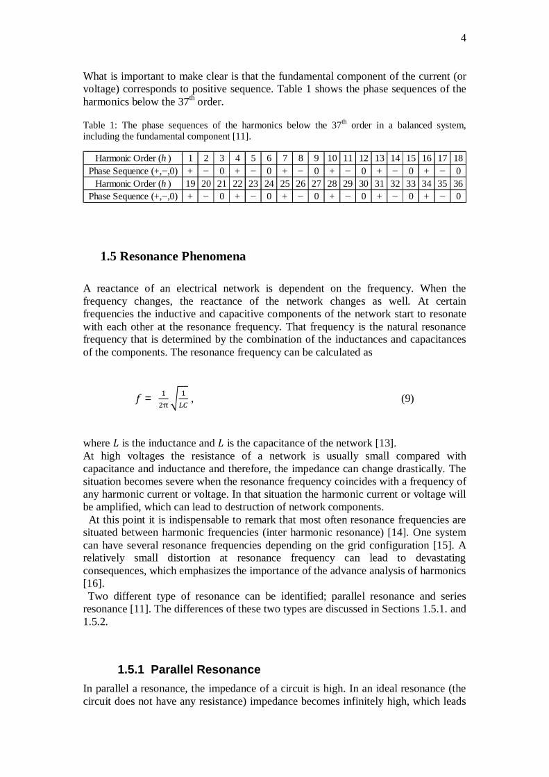
What is important to make clear is that the fundamental component of the current (or voltage) corresponds to positive sequence. Table 1 shows the phase sequences of the harmonics below the 37th order. Table 1: The phase sequences of the harmonics below the 37th order in a balanced system, including the fundamental component [11].
1.5 Resonance Phenomena
A reactance of an electrical network is dependent on the frequency. When the frequency changes, the reactance of the network changes as well. At certain frequencies the inductive and capacitive components of the network start to resonate with each other at the resonance frequency. That frequency is the natural resonance frequency that is determined by the combination of the inductances and capacitances of the components. The resonance frequency can be calculated as
= , (9)
where is the inductance and is the capacitance of the network [13]. At high voltages the resistance of a network is usually small compared with capacitance and inductance and therefore, the impedance can change drastically. The situation becomes severe when the resonance frequency coincides with a frequency of any harmonic current or voltage. In that situation the harmonic current or voltage will be amplified, which can lead to destruction of network components. At this point it is indispensable to remark that most often resonance frequencies are situated between harmonic frequencies (inter harmonic resonance) [14]. One system can have several resonance frequencies depending on the grid configuration [15]. A relatively small distortion at resonance frequency can lead to devastating consequences, which emphasizes the importance of the advance analysis of harmonics [16]. Two different type of resonance can be identified; parallel resonance and series
resonance [11]. The differences of these two types are discussed in Sections 1.5.1. and 1.5.2.
1.5.1 Parallel Resonance In parallel a resonance, the impedance of a circuit is high. In an ideal resonance (the circuit does not have any resistance) impedance becomes infinitely high, which leads
Harmonic Order (h ) 1 2 3 4 5 6 7 8 9 10 11 12 13 14 15 16 17 18Phase Sequence (+, ,0) + 0 + 0 + 0 + 0 + 0 + 0
Harmonic Order (h ) 19 20 21 22 23 24 25 26 27 28 29 30 31 32 33 34 35 36Phase Sequence (+, ,0) + 0 + 0 + 0 + 0 + 0 + 0

5
to extremely high overvoltage. At parallel resonance frequency, the voltage obtains its highest possible value at a given current. [17] Parallel resonance can occur when a source of a harmonic current is connected to the electrical circuit that can be simplified as a parallel connection of inductive and capacitive component [18]. In an extreme case, even a relatively small harmonic current can cause destructively high voltage peaks at resonance frequency [19]. Parallel resonance is common when there are capacitor banks or long AC lines connected with large transformers. In this case, large capacitances and inductances start to resonate with each other. [13]
1.5.2 Series Resonance Series resonance differs from the parallel resonance in its low impedance at a resonance frequency. At the resonance frequency the inductive and the capacitive reactance of a certain point becomes equal [12]. In this case, the capacitive reactance annuls the inductive reactance and the network impedance only consists of the resistance of the network. As the cable resistances are normally very low, the reduction of impedance can be seen as noticeably high currents [19]. The case is analogic to the parallel resonance, but instead of high voltages, high currents flow through a low impedance circuit.
2 Harmonics in a Wind Power Plant
The number of wind power plants (WPP) increases world widely and the nominal power of an average wind power plant increases. In many countries wind power has already taken an important part in the electrical energy production mix. Due to the importance of wind power, manufacturers and transmission system operators (TSO) cannot ignore the effects of wind power plants on the power quality and power system stability.
2.1 Importance of Resonance Analysis of a Wind Power Plant
Wind power plants introduce a great number of non-linear power electronic devices like full scale frequency converters into the grid. A large number of non-linear power electronic devices can have significant effect on the harmonic emissions. [20] These harmonics can form a serious threat for power quality [15]. That is why harmonic analysis has to be developed and taken as an integrated part of wind power plant design. Because every power network is unique and has different characteristics, the effect of the harmonics on every power system varies. Nevertheless, some common features can be found. Even if the percentage of the harmonics seemed small, the harmonic emission becomes a significant issue when the capacity of a wind power plant is hundreds of megawatts.

6
Emission of harmonics is not the only problem. Another problem occurs when the frequency of a harmonic current coincides with a resonance frequency. Optimal circumstances for a devastating resonance occur if some of the harmonics (or inter harmonics) coincides with the network resonance frequency. [21] The components that make the power system more likely to experience resonances are discussed in Section 2.4.
2.2 Direct Harm Caused by Harmonics
Harmonics have many kinds of adverse effects in a power network. The major part of the components used in power networks is mainly designed for the fundamental frequency. Many times, the components operate in conditions that do not form an optimal operating environment, which can have adverse effects on the components. Harmonic emissions are a commonly recognised problem in wind power plants. [22], [23] Probably the most significant problem is that harmonic currents cause overheating and extra losses in many components, like cables, capacitor banks, generators, transformers, reactors and any kinds of electronic equipment. Overheating shortens their useful lifetime, and in an extreme case, can lead to the destruction of some component, especially in the case of capacitor banks. [24] When a power system has components with large a capacitance or inductance, the probability of the existence of resonances increases, as explained before. If harmonic currents or voltages are high enough, they can provoke an unnecessary tripping of protective relays [2]. They can also degrade the interruption capability of circuit breakers [1]. If the filtering is not well designed, harmonics may cause adverse effects on the measuring devices that are not made for taking into account the existence of distorted waveforms. These malfunctions can have an effect on measured results although devices might be equipped with filters. [2] The functioning of many electronic devices is based on the determination of the shape of voltage waveform, for example detecting the zero-crossing point. As harmonic distortion can shift this point, the risk of system malfunction is evident [25]. Especially important is to mention the drawback of harmonics on impedance measurement that is used in distance relays [26]. The power transferred in power networks and communication networks is in a totally different scale (megawatt versus milliwatt), so even a relatively small amount of current distortion in the power network can easily provoke significant noise in a metallic communication circuit at harmonic frequencies [1].
2.3 Harmonic Sources in a Wind Power Plant
In modern wind power plants a huge number of different power electronic apparatus is installed, which is the main reason for harmonics in the wind power plants. The switching operations of the pulse width modulation (PWM) controlled converters are
7
the main sources of harmonic and inter harmonic currents, but not the only ones. Generally speaking, converters create harmonics in the range of a few kilohertz. [27] Measuring and controlling these harmonics is one of the greatest challenges of the
power quality in wind power plants. [28] The next sections present the most significant types of harmonic sources.
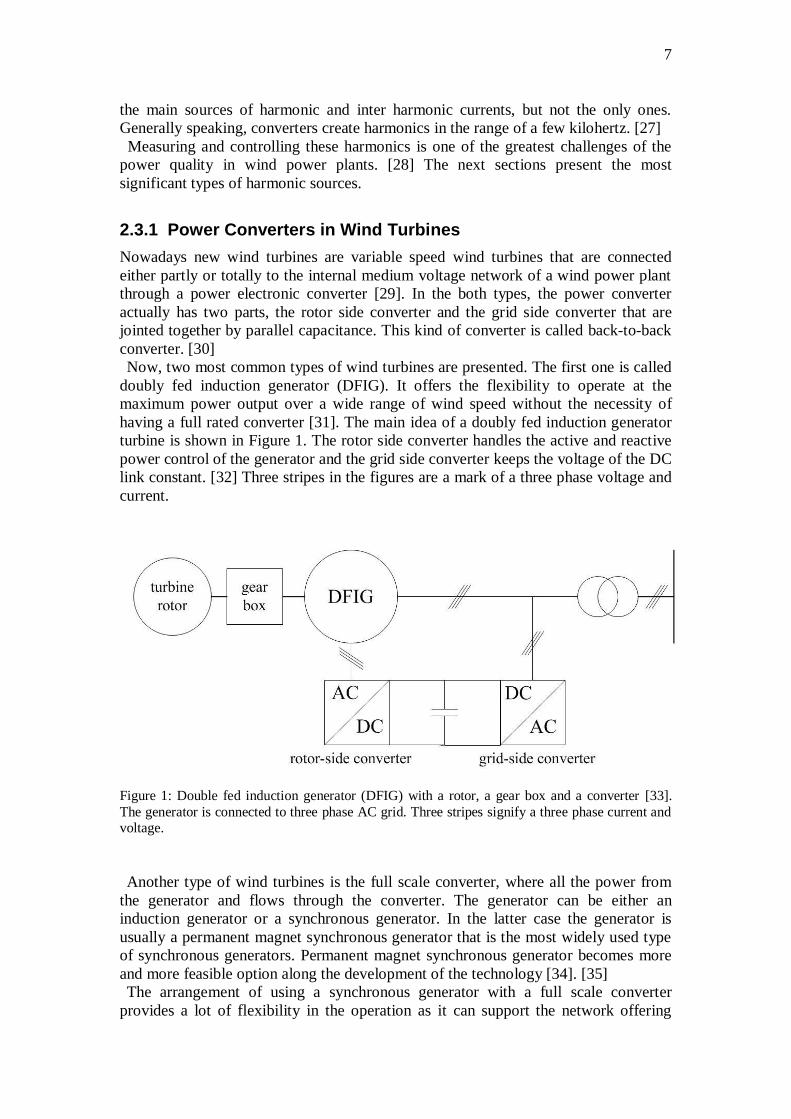
2.3.1 Power Converters in Wind Turbines Nowadays new wind turbines are variable speed wind turbines that are connected either partly or totally to the internal medium voltage network of a wind power plant through a power electronic converter [29]. In the both types, the power converter actually has two parts, the rotor side converter and the grid side converter that are jointed together by parallel capacitance. This kind of converter is called back-to-back converter. [30] Now, two most common types of wind turbines are presented. The first one is called
doubly fed induction generator (DFIG). It offers the flexibility to operate at the maximum power output over a wide range of wind speed without the necessity of having a full rated converter [31]. The main idea of a doubly fed induction generator turbine is shown in Figure 1. The rotor side converter handles the active and reactive power control of the generator and the grid side converter keeps the voltage of the DC link constant. [32] Three stripes in the figures are a mark of a three phase voltage and current.
Figure 1: Double fed induction generator (DFIG) with a rotor, a gear box and a converter [33]. The generator is connected to three phase AC grid. Three stripes signify a three phase current and voltage. Another type of wind turbines is the full scale converter, where all the power from
the generator and flows through the converter. The generator can be either an induction generator or a synchronous generator. In the latter case the generator is usually a permanent magnet synchronous generator that is the most widely used type of synchronous generators. Permanent magnet synchronous generator becomes more and more feasible option along the development of the technology [34]. [35] The arrangement of using a synchronous generator with a full scale converter
provides a lot of flexibility in the operation as it can support the network offering

8
reactive power even if there was not wind at all [36]. An arrangement of a synchronous generator with a full scale converter is shown in Figure 2.
Figure 2: A full scale converter configuration with a turbine rotor, a gear box, a generator (G) and a back-to-back converter [20]. The generator is connected to three phase AC grid. Three stripes signify a three phase current and voltage. The harmonic emissions of wind turbines can be classified as characteristic and non-characteristic harmonics. The characteristic harmonics depend on the converter topology and switching strategy used during an ideal operation (with no disturbances). For a six-pulse converter, the characteristic harmonics are the harmonics of the harmonic order 6 ± 1, where is a positive integer. Similarly for a twelve-pulse converter the characteristic harmonics are of the order 12 ± 1. [37] Apparently, the non-characteristic harmonics are the harmonics that are not counted
as characteristic harmonics. They are not depending on the converter topology, but the operating point of the converter [38]. This type of harmonics can be as large and as significant as the characteristic harmonics [39].
2.3.2 Voltage Source Converter High Voltage Direct Current Links Voltage source converter high voltage DC links are coming more and more popular as connections between an off shore transformer and an on shore substation [40]. With the help of this technology, the level and the direction of the power flow can be controlled quickly. Mostly voltage source converter high voltage DC converters utilize two-level topology, but the multi-level and the multi-pulse converters are becoming more and more attractive options due to their lower harmonic emission levels [41], [42]. The multi-pulse converters are made by connecting several six-pulse converters in parallel [43]. The low order harmonics are deleted proportionally to the increment in pulse numbers [44].
2.3.3 Flexible Alternative Current Transmission System Devices Flexible AC transmission systems is a large family of devices of a different kind that are used for controlling active and reactive power, increase voltage stability and reduce losses in the network [45]. In wind parks, the static var compensator (SVC) and the static synchronous compensator is the most widely used types of Flexible AC transmission systems apparatus. A static var compensator includes three parts: a thyristor-controlled reactor, a
thyristor-switched capacitor and a harmonic filter. A typical configuration of a static

9
var compensator is shown in Figure 3. It has its maximum capacitive and reactive power limits and it is able to operate within those limits. Usually, a static var compensator is installed at the collector bus of a wind power plant where it adjusts its reactive power output to support the network (for example in a sudden voltage dip). A static var compensator can solve most of the steady state voltage problems. A static var compensator injects harmonics to the network and that is why it has to be equipped with a filter. [46], [47]
Figure 3: Typical configuration of SVC [48]. Three stripes signify a three phase current and voltage. The filter is connected to three phase AC grid. TCR signifies thyristor-controlled reactor and TSC thyristor-switched capacitor. A static synchronous compensator consists of a voltage source or a current source
converter and an energy storage (sometimes used without an energy storage unit) as in Figure 4 [49]. A static synchronous compensator supports the grid when supplemental reactive power is needed. Compared with a static var compensator, a static synchronous compensator has quicker response time, smaller size and ability to provide active power (if it is equipped with energy storage). At the same voltage rate it has a capability to provide more reactive power than a static var compensator. The harmonic production of a static synchronous compensator depends on the topology of the converter, the switching frequency of the thyristors and the pulse pattern used. The higher is the number or the pulses, the more harmonics can be eliminated. [46], [50], [51], [52], [49]

10
Figure 4: A voltage source converter-based static synchronous compensator without energy storage [49]. The compensator is connected to three phase AC grid. Three stripes signify a three phase current and voltage.
2.4 Increasing the Possibility of Harmonic Resonances
All wind parks are unique. They all have their own resonance frequencies that are dependent on the grid topology, connected generators and reactive power apparatus used. [21] Furthermore, the impedance and the resonance points of a wind park change all the time when the number of turbines and capacitor banks in operations changes or when there are changes in the connections of collector cables [20]. The more turbines the wind park has, the more the impedance can vary. The topic is especially important in large off shore wind parks, where the number of
turbines in function can vary from a few to many hundreds. Moreover, off shore wind farms are connected with long cables that have large capacitance. [53] In the following sections, some of the most important components due to impedance
changes are discussed.
2.4.1 Cable Connections Cable connections in wind parks can be divided into two groups: an internal collector cable system of a wind power plant that connects the turbines of the wind park with each other and a transmission cable that connects the wind park to substation, many times located on shore. The total length of the collector cable system varies in different kinds of off shore wind power plants from a few kilometres until tens of kilometres. The widespread submarine collector cable network can bring a large capacitance in the system. [15] Underwater cables have to be resistant, and consequently well armoured [94]. The
11
armouring affects significantly the impedance and the frequency response of underwater cables [54]. The connection cable is another large capacitance that can magnify harmonic currents or voltages that are near the resonance frequency [16]. The connection may be an AC or a DC cable depending on transferred distance. Naturally, these two options have different effect on resonance frequencies. The DC connection cable can have the distance even up to 100 kilometres [55]. Harmonic resonance is one of the main technical challenges in the design and operation of off shore distribution system [25].
2.4.2 Capacitor Banks and Reactors Several capacitors connected together as capacitor banks are commonly used to compensate reactive power and to help improving the power factor. Many times, there is a capacitor bank at each turbine as well as at the point of common coupling (PCC). [56] The capacitor banks in the individual turbines are used also to support the voltage in sudden dips that may occur in harsh wind conditions [15]. Large wind power plants with even hundreds of turbines have a great number of different switching options for the capacitor banks. There can be shunt reactors connected to transmission cable terminations to
compensate the high capacitance of the cables. These reactors are inductive components that may be adjustable and equipped with a tap changer. The reactors can be connected to the same switch together with the cable connection. [57]
2.5 Harmonics Mitigation in a Wind Power Plant
There are two fundamental strategies for avoiding harmonics in wind power plants. The first one is to design the wind power plant and its components in a way that they do not produce harmonics. The second strategy is to use filters to filter out the harmonics. The second way is more common since the preventive method is not always possible. [58]
2.5.1 Preventive Manners Converters form the main source of harmonic currents and a decrease in the injection converter harmonics has a positive effect on total harmonic distortion in a wind power plant. One technique to achieve the reduction of the level of harmonics emitted by the converters is to increase the pulse number of the converters. The higher is the pulse number, the less harmonics are emitted. Another way to prevent the harmonics created in the converters is to use multi-level topology. [59] Another common method is to use a phase shifting transformer in each wind turbine to prevent the flow of harmonics into the medium voltage (usually between 10 kV and 33 kV) collector grid. The idea is to bring the harmonic currents phase shift of 180o and the harmonic currents delete each other. For example, delta-wye connected
12
transformer deletes the even harmonics, the third one and its multiples, so there are only harmonics of the order 5th, 7th, 11th, 13th, 17th and so on. [60], [61]
2.5.2 Harmonic Filters There are basically three types of filters used to mitigate harmonics. They can be classified as passive, active and hybrid filters. The following sections provide a brief description is of all of them.
2.5.2.1 Passive Filters Passive filters consist of capacitances, inductances and resistances tuned to damp harmonics. A significant disadvantage of the passive filters is that they can start to resonate together with the surrounding network elements. The most common type of passive filter is the parallel or the shunt passive filter. It is also named as the damped filter. It has a capacitor connected in series with a parallel connection of an inductor and a resistor, as shown in Figure 5. It provides a low impedance path for the tuned harmonic frequency and this way they trap the harmonic and damp it. Another general type of passive filter is the series passive filter. As its name
indicates, it is connected is series with the load. It includes an inductor and a capacitor that are connected in parallel. The components are tuned to provide a high impedance path for a selected harmonic frequency and a very low impedance path for the fundamental frequency. With this arrangement, the filter blocks the tuned frequency and does not affect the fundamental current. [11], [62] When talking about the series filters, one constraint is that they must withstand the
full current and they must be insulated for full line voltage, unlike the parallel or shunt filters that carry just a fraction of the full current. Moreover, the parallel filters provide reactive power for the grid at fundamental frequency. [63]

13
Figure 5: A passive shunt filter [63], [61], [58]. Three stripes signify a three phase current and voltage. R is a resistor, C is a capacitor and L is an inductor. The filter is connected to three phase AC grid.
2.5.2.2 Active Filters Active filters can be connected in parallel or in series with the load. The principal idea of their operation is that they inject current that is opposite in phase with the harmonics of the fundamental current. This way they eliminate the harmonic components from the fundamental current. [64] Nowadays the active filters show a significantly better performance in comparison with the passive filters. The advantages are that they can be programmed to block several orders of harmonics instead of just one and they can also provide reactive power when needed or they can be used to compensate the neutral current. [65] Moreover, the active filters do not have the danger of resonating with other network components as the passive filters. [66] The cost of the high power rated converter is the greatest disadvantage of the active filters although the prices are decreasing. [67], [68]
2.5.2.3 Hybrid Filters There is a great variety of different kinds of hybrid filters. They all try to achieve a high performance in the elimination of harmonics while minimizing the costs by combining an active and a passive filter. [68], [69], [70] Figure 6 shows one possible configuration of the hybrid filter. Any detailed classification of the hybrid filters is out of the scope of this thesis.

14
Figure 6: A hybrid filter in an industrial network [71]. Three stripes signify a three phase current and voltage. L is an inductor and C is a capacitor. The filter is connected to three phase AC grid.
2.6 Limits of German Electricity Association for Harmonic
Currents
German Electricity Association (Verband der Elektrizitätswirtschaft, VDEW) has set standard values for harmonic currents stemming from grid connected converters. These values are indispensables in the design process of output filters of converter for wind turbines [72]. The allowed amount of harmonic current is dependent on the voltage level, the short circuit power of the network and the rated output power of the converter. Table 2 shows constants for the voltage levels of 10 kV and 20 kV. The maximum harmonic current limits (separately for each harmonic) allowed can be calculated by multiplying these constants by the short circuit ratio of the network at the connection point as
, = , , (10)

15
where , is a constant from Table 2 and is the short circuit power of the network. [73] Table 2: German Electricity Association constants to calculate maximum allowed limits for each harmonic current. The maximum allowed limits for the harmonic currents can be calculated by multiplying the constants by the short circuit power of the network where a converter is connected. [73]
Constants for calculating the maximum allowed harmonic currents for any other voltage level can be calculated by using the constant values of Table 2 as they are inversely proportional to the voltage level. To calculate limits for triple harmonics as well as for harmonics up to 25th order the constant of the next harmonic must be used within the condition that the zero sequence currents are not routed into the grid. There are also other organizations, like IEEE, that give limits for injected harmonics related to the converters but their introduction is out of the scope of this project. [73], [74]
3 Computation Technique of Harmonic Analysis
This chapter explains the mathematical backgrounds of two methods for identifying resonances in electrical networks. The first method is called the frequency scan (or the impedance scan) and the second method is the harmonic resonance mode analysis. Both of these methods are used in the simulations of Chapter 4. Section 3.2.3 explains how these two methods are linked together.
Harmonic Order
h 10 kV Network 20 kV Network5 0.115 0.0587 0.082 0.041
11 0.052 0.02613 0.038 0.01917 0.022 0.01119 0.018 0.00923 0.012 0.00625 0.01 0.005
h > 25 and Pairs 0.06/h 0.03/hh < 40 0.06/h 0.03/h
h > 40* 0.18/h 0.09/h* Integer and not integer within a bandwidth of 200 Hz
The Constants for Calculating the Allowed Rated for Harmonic Currents

16
Traditionally, harmonic analysis has two steps; the first one is the frequency scan that is made to identify the resonance frequencies and the second step is to calculate the harmonic distortions at the buses of interest [29].
3.1 Frequency Scan
The frequency scan is also called the impedance scan, the current source method and the impedance sweep [13]. It is normally the first step of the harmonic analysis. Its principal objective is to detect the possible resonance frequencies in the electrical network [29]. The frequency scan is performed of one bus at the time. A sinusoidal current with the amplitude of 1 per unit and with a certain frequency (the frequency of interest) is injected into this bus and the corresponding voltages from the following equation are calculated as
[ ] = [ ] [ ], (11)
where [ ] is the network admittance matrix, [ ] harmonic current matrix and [ ] harmonic voltages and the subscript h denotes the harmonic order. [75] The diagonal entries of the [ ] matrix are called the driving point admittances and correspondingly the diagonal entries of the impedance matrix (the inverse of the admittance matrix) are called the driving point impedances [76]. The impedance seen at a bus is calculated at all frequencies, sweeping or scanning the frequency spectrum of interest. The result of this calculation is a plot (a curve) of the magnitude of the impedance seen from the bus (on the vertical axis) versus the harmonic frequency (or the harmonic order) (on the horizontal axis). [1] The frequency scan can be applied on both one phase and three phase systems. When applied on three phase systems, the entries of the admittance matrix are 3 matrices that include self- and transfer admittances between three phases. [1] The method is very illustrative, as it clearly shows the points of resonance. A dip in
the impedance plot signifies a series resonance and a sharp peak in the impedance curve refers to a parallel resonance at this frequency [53]. This is coherent with the resonance theory that says that in the ideal theoretical case the impedance at the parallel resonance becomes infinitely large and at the series resonance the impedance is limited to the value of the resistance [18]. Although, the frequency scan is very useful for finding the resonances of any
network, it has its limits. It does not indicate which of the systems components causes the resonance and where is the best location to control the resonance. [75] Alternatively, instead of injecting a current with a value of a 1 per unit, a voltage with a value of 1 per unit can be injected into one of the buses of the network. Similarly, a voltage versus frequency in the remaining points of the network is calculated. The peaks in the curve tell at which frequencies the voltages are magnified and, vice versa, the dips indicate at which frequencies the voltages are damped. This method is called a voltage scan or a voltage transfer function study. [77] One major challenge with the frequency scan analysis is to cover the enormous number of different system configurations. Although a single calculation is not
17
difficult, the great number of calculations that have to be evaluated makes the task laborious. In practice, this is performed by executing the frequency scan for several configurations and showing the results in a so-called contour plot, where the harmonic number is shown as a function of turbines in operation. [58]
3.2 Harmonic Resonance Mode Analysis
To give a broader picture that the frequency scan offers about a resonance problem there is an alternative method called harmonic resonance mode analysis (HRMA), resonance mode analysis (RMA) or simply modal analysis. It overcomes some restrictions that frequency scan has. This technique is based on the similar manipulation of the network admittance matrix [ ] that has been used for a long time in the investigation of power systems small signal stability. These well-known techniques can be utilized in the resonance studies. [78] The harmonic resonance mode analysis is designed for identifying parallel resonances, which is usually the most critical form of resonance (see Section 1.5) [79]. Harmonic resonance mode analysis is based on the fact that the admittance matrix of
a power network becomes singular, at resonance frequencies. Singularity of an admittance matrix means that its determinant is zero. It happens when one of the eigenvalues of an admittance matrix is zero. [80] Equation (12) shows that high nodal voltages occur when the admittance matrix comes closer to its singularity (when the eigenvalues in the diagonal eigenvalue matrix have very small values) [81]. In the equations the subscripts of the harmonic orders can be used as in Equation (11), but here the subscripts are left out to make the equations easier to read. The admittance matrix can be decomposed into three components as follows
[ ] = [ ][ ][ ], (12)
where [ ] is the left eigenvector matrix, [ ] is the right eigenvector matrix and [ ] is the diagonal eigenvalue matrix, that has the eigenvalues of the admittance matrix [ ] in the diagonal entries. To avoid confusions, one should keep in mind that usually in mathematics, the right eigenvector matrix is called the eigenvector matrix [80]. What is important to mention is that the left eigenvector matrix is the inverse of the right eigenvector matrix as
[ ] = [ ] . (13)
If we combine Equation (12) with Equation (13), we get the following:
[ ] = [ ][ ] [ ][ ]. (14)

18
Equation (14) shows the harmonic voltages at certain bus as a result of harmonic current injection. In Equation (15), the vector [ ] contains the harmonic currents and the vector [ ] contains the harmonic voltages as
[ ][ ] = [ ] [ ][ ]. (15) Equation (15) can be simplified as,
[ ] = [ ] [ ], (16) if it is said that [ ] = [ ][ ] is the modal voltage vector and [ ] = [ ][ ] is the modal current vector. [79], [82] The inverse of the eigenvalue is called modal impedance ( ) as its unit is ohm. The
smaller the eigenvalue (the greater the modal impedance) is, the greater is the harmonic resonance and therefore, the mode with the smallest eigenvalue (and highest modal impedance) is called critical mode. The result is that resonances occur at particular modes. [83], [84] There is a certain analogy to power system small signal stability analysis, as the right
eigenvector of the critical mode shows the controllability (or excitability) and the corresponding left eigenvector tells the observability of the critical mode [85], [86]. Since the harmonic resonance mode analysis can identify only the parallel resonances of an electric network, there is a similar method that is designed to identify series resonances. That method is identical to the harmonic resonance mode analysis, but instead of manipulating the nodal admittance matrix it the loop impedance matrix is manipulated. [87], [79] According to the experience of the author, the efficiency and the accuracy of the method is not clear yet and it is discarded in this thesis.
3.2.1 Sensitivity Matrix Harmonic resonance mode analysis can be used with modal sensitivity analysis that means investigating the effect of the entries of the admittance matrix on its eigenvalues. That is performed by constructing a sensitivity matrix. [88] An admittance matrix of the size (at any frequency) has eigenvalues and each of them corresponds to one right eigenvector and one left eigenvector. So, the kth eigenvalue has the corresponding right eigenvector and the corresponding left eigenvector . If is a network component parameter (for example the capacitance of a capacitor), the eigenvalue sensitivity with respect to this parameter is the admittance matrix sensitivity to this parameter. This is demonstrated as
= , (17) where Y is the admittance matrix. [75]

19
We can find the sensitivity of the kth eigenvalue with respect to the entries of the admittance matrix from the sensitivity matrix of size , which is calculated by multiplying the first column of the right eigenvector matrix by the first row of the left eigenvector matrix, as
= = . (18)
In Equation (18), the diagonal entries of the sensitivity matrix are called participation factors. The participation factors indicate how strongly each bus of the network is involved in the resonance at each mode. Since the right eigenvectors show the controllability and the left eigenvectors show the observability at a certain frequency, the participation factors indicate the bus where the controllability and the observability are optimized. Therefore, the participation factors indicate the location where any possible harmonic mitigation activities should be considered. [82], [78] Moreover, the magnitude of the participation factor shows how far the resonance emanates [87].
3.2.2 Eigenvalue Sensitivities with Respect to Power System Components
We can also have the eigenvalue sensitivities with respect to certain components. In other words, we can calculate the effect of a certain component on a designated eigenvalue. Here the equations are shown, but not conducted. For a shunt component at bus with admittance can be said that the sensitivity the of kth eigenvalue with respect to this component is the same as the eigenvalue sensitivity with respect to a certain bus or a bus participation factor
= , . (19)
That is logical since any shunt component affects only one entry of the admittance matrix. The case is slightly more complicated with series components since any series component has some effect on four entries in the admittance matrix. The kth eigenvalue sensitivity with respect to series component is
= , + , , , , (20)
where is the admittance of a series component that situates between the buses and . On the right side of the equation are the four entries of the sensitivity matrix. [75], [82]
20
3.2.3 The Connection between Modes and Impedances of the Frequency Scan
The impedance curves from the frequency scan are not exactly the same as the modal impedances that are given by the modal analysis. Although, the results from both calculations refer to the same physical phenomena, there is a slight difference as the results of the frequency scan can be seen as a composition of modes and participation factors. The impedance that is seen from the bus in the frequency scan is expressed as
= + + . (21) In Equation (21), is participation factor, is modal impedance and refers to the number of modes. [85] Equation (21) shows that does not always reach its maximum point when one of the modal impedances reaches its maximum point, since there are several modal impedances affecting [85]. Here, the important role of the participation factors can be seen clearly as they determine how much each mode (or modal impedance) takes part in the impedance seen from a particular bus.
4 Simulations – Aggregated Wind Power Plant
In this part of the thesis, resonance conditions and harmonics are studied based on simulations of an aggregated model of an off shore wind power plant. Section 4.1 explains how the wind power plant is modelled for the study of harmonics and resonances. In Section 4.2, the modal analysis and the frequency scan are performed for the wind power plant. Section 4.3 and 4.4 study how a change in the length of the collector cables and the transmission cables affects the resonance points of the wind power plant. After having an insight into the resonances of the wind power plant the effect of a passive and a hybrid filter on resonance conditions is studied (Sections 4.5 and 4.6). Section 4.7 analyses the harmonic current and voltages performed in cases without any filters and with passive filters. Section 4.8 studies the impact of skin effect on the modal analysis. Except this part, the results of the modal analysis as well as the results of the frequency scan are provided in all cases. MATLAB is used to calculate the modal analyses and PSCAD software to carry out the frequency scans. Some of the results in this chapter are in Appendices A and B in order to make the text more readable. It is indicated in text and in caption, if part of the information is in appendix.

21
4.1 Modelling the Wind Power Plant
In the simulations of this thesis, an aggregated model of a 400 MW wind power plant is used as in Figure 7. Each individual wind turbine is not modelled rather the turbines are presented as four large aggregated turbines, each of them situated at the end of one branch. Every turbine represents the power of 100 MW. Each of these four aggregated wind turbine models consists of a permanent magnet synchronous generator, a full scale converter, an LCL (inductance capacitance inductance) filter, and a generator transformer. Wind turbines (and converters) are connected to collector buses though 8 kilometres long 33 kV submarine collector cables. The collector cables are connected to 58 kilometres long 150 kV transmission cables through a three winding transformer with YNdd configuration that eliminates the zero sequence harmonics. Zigzag transformers are used for earthing the 33 kV collector cable network. On the grid side of the 150 kV cables there is a converter transformer to adjust the voltage to the voltage source converter of the high voltage DC connection. Between the high voltage DC converter and the 150 kV bus, there is a tuned filter and a phase reactor. A layout of the wind power plant is presented in Figure 7.
Figure 7: Layout of the aggregated wind power plant [88]. The figure is used with the permission of the author. Figure 8 shows how the system is modelled for the resonance studies. The parameters of the components are in Table 3. All the cable connections are modelled as -branches. All the transformers and reactors are modelled as series inductances. The possible saturation of the transformers is not taken into account, since this is sufficient for the majority of harmonic studies [89]. The zigzag transformers are excluded from the harmonic analysis. The tuned filter that is in parallel with the phase reactor and the high voltage DC connection is modelled as a capacitance, as in [89]. All the components of the network are reduced to 150 kV level. The harmonic analyses are performed below the 26th harmonic. All the frequency-dependent results are shown in per units rather than frequency as the per unit values are easy to perceive. The per unit value of the frequency is the same as harmonic order.

22
The components of the aggregated model of the wind power plant are shown in Figure 8 and the values of the components are in Table 3.

23
Figure 8: The model of the wind power plant used. WTG signifies wind turbine generator. The four branches are indicated clearly.

24
Table 3: The parameters of the components in the model, where all values are reduced to the 150 kV voltage. The names of the components can be seen in Figure 8.
4.2 Resonance Analysis of the Wind Power Plant
The wind power plant of Figures 7 and 8 is represented in the modal analyses, as a grid with 20 buses, or nodes, as presented in Figure 9. All of the buses are not real buses of the power system; rather they are nodes that help to spot the locations of the possible resonances.
Component The Name of Component Electrical Value
Phase reactor Lr 19.3 mHThe capacitance of the tuned filter
C1 5.658 E 6 F
Converter transformers Lt1 19.338 mH150 kV Cables Ztrans1, Ztrans2 - Series resistance 0.056 - Series inductance 1.0 mH - Shunt capacitance 0.52 E 6 FThree winding transformers Lt21, Lt22, Lt23, Lt24 38.676 mH33 kV Cables Ztrans11, Ztrans12, Ztrans21,
Ztrans22 - Series resistance 0.372 - Series inductance 18.181 mH - Shunt capacitance 5.709 E 8 FGenerator transformer Lt31, Lt32, Lt33, Lt34 51.568 mHLCL Filter - Wind turbine side Lf21, Lf22, Lf23, Lf24 1.2 H - Capacitor Cf11, Cf12, Cf13, Cf14 1.491 E 7 F - Grid side Lf11, Lf12, Lf13, Lf14 0.641 H

25
Figure 9: The wind power plant as it is used in the modal analyses. The model consists of 20 buses. The modal analysis is performed by finding the smallest eigenvalues of the admittance matrix (see Equation 12). The modal impedances are obtained by calculating the inverse of each eigenvalue. The frequencies of all the modal impedance peaks (the resonance frequencies) are found according to the explanation in Section 3.2. The bus participation factors are obtained by manipulating the admittance matrix at these frequencies. A detailed explanation of the modal analysis can be found in Section 3.2. Figure 10 shows the four most critical modes as a result of modal analysis. The horizontal axis (the values of X) shows the frequency in per units (the harmonic order) and the vertical axis (the values of Y) represents the absolute value of the modal impedance. The black curve with two peaks represents the critical mode, which is the mode with the highest modal impedance (see the first column of Table 4). The bus participation factors are presented in Table 4. Each column of the participation factor tables (as Table) represents one mode. In these tables the modes are arranged in the order of their criticality (the critical mode first, the second critical mode second, etc.). In addition, the harmonic order and the frequency of each modal impedance peak as well as the maximum value of the peak are shown. The number of mode in Tables 4 refers to the order in which MATLAB algorithm
ranks the eigenvalues. The order is dependent on the algorithm that is used to
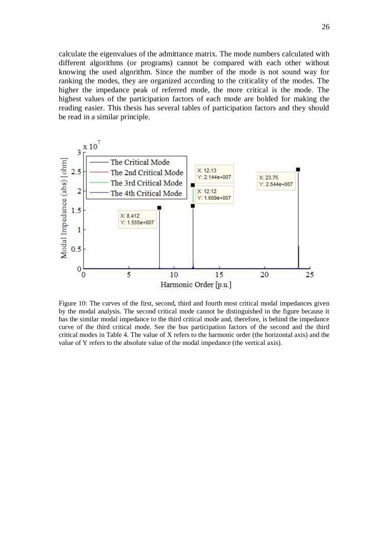
26
calculate the eigenvalues of the admittance matrix. The mode numbers calculated with different algorithms (or programs) cannot be compared with each other without knowing the used algorithm. Since the number of the mode is not sound way for ranking the modes, they are organized according to the criticality of the modes. The higher the impedance peak of referred mode, the more critical is the mode. The highest values of the participation factors of each mode are bolded for making the reading easier. This thesis has several tables of participation factors and they should be read in a similar principle.
Figure 10: The curves of the first, second, third and fourth most critical modal impedances given by the modal analysis. The second critical mode cannot be distinguished in the figure because it has the similar modal impedance to the third critical mode and, therefore, is behind the impedance curve of the third critical mode. See the bus participation factors of the second and the third critical modes in Table 4. The value of X refers to the harmonic order (the horizontal axis) and the value of Y refers to the absolute value of the modal impedance (the vertical axis).

27
The C
ritic
ality
of M
ode
12
34
56
78
910
1112
1314
1516
1718
1920
The N
umbe
r of
Mod
e7
1920
149
815
1716
1018
1211
136
53
42
1Ha
rmon
ic Or
der [
p.u.]
23.75
12.13
12.13
12.12
12.32
8.41
12.12
12.13
12.11
12.36
12.62
12.99
13.17
13.56
12.32
10.99
10.99
13.95
18.17
25.00
Freq
uenc
y [Hz
]11
87.35
606.4
606.4
605.8
561
6.15
420.6
560
5.860
6.560
5.65
617.8
631
649.2
565
8.55
677.9
616.1
554
9.754
9.769
7.690
8.612
50Th
e Max
imum
Ab
solu
te Va
lue
of M
odal
Impe
danc
e []
2.544
E+07
2.144
E+07
2.144
E+07
1.609
E+07
1.582
E+07
9.963
E+06
8.244
E+06
5.156
E+06
2.612
E+06
2.721
E+05
2.275
E+04
1.443
E+04
1.144
E+04
8.097
E+03
1.931
E+03
1.311
E+03
2.376
E+02
1.979
E+02
6.437
E+01
2.596
E+00
Bus
Parti
cipati
on
Facto
rs Bus 1
0.003
60.0
000
0.000
00.0
000
0.005
30.0
290
0.000
00.0
000
0.000
00.0
052
0.000
00.0
035
0.003
10.0
025
0.111
60.1
631
0.66
470.7
207
0.942
20.0
002
Bus 2
0.061
00.0
000
0.000
00.0
000
0.000
70.0
445
0.000
00.0
000
0.000
00.0
007
0.000
00.0
001
0.000
10.0
000
0.079
80.0
912
0.087
00.0
776
0.021
50.6
642
Bus 3
0.063
20.0
000
0.000
00.0
000
0.000
60.0
448
0.000
00.0
000
0.000
00.0
006
0.000
00.0
001
0.000
00.0
000
0.078
70.0
893
0.079
90.0
705
0.017
00.1
678
Bus 4
0.070
50.0
014
0.000
10.0
008
0.000
00.0
471
0.000
80.0
012
0.000
80.0
000
0.001
40.0
003
0.000
40.0
006
0.056
60.0
551
0.014
20.0
103
0.000
50.0
000
Bus 5
0.070
00.0
031
0.000
30.0
016
0.000
20.0
478
0.001
60.0
026
0.001
60.0
002
0.003
00.0
008
0.000
90.0
013
0.050
10.0
459
0.006
40.0
041
0.000
10.0
000
Bus 6
0.057
70.0
108
0.001
00.0
054
0.002
60.0
490
0.005
40.0
091
0.005
40.0
026
0.010
80.0
038
0.004
10.0
046
0.040
10.0
331
0.001
60.0
008
0.000
00.0
000
Bus 7
0.004
00.4
995
0.044
20.2
422
0.245
40.
0653
0.242
20.4
187
0.242
20.2
454
0.523
50.2
442
0.243
80.2
429
0.015
90.0
076
0.000
00.0
000
0.000
00.0
000
Bus 8
0.070
50.0
014
0.000
10.0
008
0.000
00.0
471
0.000
80.0
012
0.000
80.0
000
0.001
40.0
003
0.000
40.0
006
0.056
60.0
551
0.014
20.0
103
0.000
50.0
000
Bus 9
0.070
00.0
031
0.000
30.0
016
0.000
20.0
478
0.001
60.0
026
0.001
60.0
002
0.003
00.0
008
0.000
90.0
013
0.050
10.0
459
0.006
40.0
041
0.000
10.0
000
Bus 1
00.0
577
0.010
80.0
010
0.005
40.0
026
0.049
00.0
054
0.009
10.0
054
0.002
60.0
108
0.003
80.0
041
0.004
60.0
401
0.033
10.0
016
0.000
80.0
000
0.000
0Bu
s 11
0.004
00.4
995
0.044
20.2
422
0.245
40.
0653
0.242
20.4
187
0.242
20.2
454
0.523
50.2
442
0.243
80.2
429
0.015
90.0
076
0.000
00.0
000
0.000
00.0
000
Bus 1
20.0
632
0.000
00.0
000
0.000
00.0
006
0.044
80.0
000
0.000
00.0
000
0.000
60.0
000
0.000
10.0
000
0.000
00.0
787
0.089
30.0
799
0.070
50.0
170
0.167
8Bu
s 13
0.070
50.0
001
0.001
40.0
008
0.000
00.0
471
0.000
80.0
007
0.000
80.0
000
0.000
10.0
003
0.000
40.0
006
0.056
60.0
551
0.014
20.0
103
0.000
50.0
000
Bus 1
40.0
700
0.000
30.0
031
0.001
60.0
002
0.047
80.0
016
0.001
50.0
016
0.000
20.0
002
0.000
80.0
009
0.001
30.0
501
0.045
90.0
064
0.004
10.0
001
0.000
0Bu
s 15
0.057
70.0
010
0.010
80.0
054
0.002
60.0
490
0.005
40.0
053
0.005
40.0
026
0.000
80.0
038
0.004
10.0
046
0.040
10.0
331
0.001
60.0
008
0.000
00.0
000
Bus 1
60.0
040
0.044
20.4
995
0.242
20.2
454
0.06
530.2
422
0.243
60.2
422
0.245
40.0
394
0.244
20.2
438
0.242
90.0
159
0.007
60.0
000
0.000
00.0
000
0.000
0Bu
s 17
0.070
50.0
001
0.001
40.0
008
0.000
00.0
471
0.000
80.0
007
0.000
80.0
000
0.000
10.0
003
0.000
40.0
006
0.056
60.0
551
0.014
20.0
103
0.000
50.0
000
Bus 1
80.0
700
0.000
30.0
031
0.001
60.0
002
0.047
80.0
016
0.001
50.0
016
0.000
20.0
002
0.000
80.0
009
0.001
30.0
501
0.045
90.0
064
0.004
10.0
001
0.000
0Bu
s 19
0.057
70.0
010
0.010
80.0
054
0.002
60.0
490
0.005
40.0
053
0.005
40.0
026
0.000
80.0
038
0.004
10.0
046
0.040
10.0
331
0.001
60.0
008
0.000
00.0
000
Bus 2
00.0
040
0.044
20.4
995
0.242
20.2
454
0.06
530.2
422
0.243
60.2
422
0.245
40.0
394
0.244
20.2
438
0.242
90.0
159
0.007
60.0
000
0.000
00.0
000
0.000
0
Tabl
e 4:
The
bus
par
ticip
atio
n fa
ctor
s fro
m th
e ha
rmon
ic re
sona
nce
mod
e an
alys
is. A
ll of
the
20
mod
es a
re p
rese
nted
. The
hig
hest
val
ues
of th
e pa
rtici
patio
n fa
ctor
s of e
ach
mod
e ar
e bo
lded
.

28
Figure 11: The impedance given by the frequency scan is calculated at buses 1–7. See the order of the buses in Figure 9.
12.1 p.u., 354842
23.7 p.u., 23281
12.1 p.u., 7978
8.4 p.u., 34404
0
5000
10000
15000
20000
25000
30000
35000
40000
0 1 2 3 4 5 6 7 8 9 10111213141516171819202122232425
Impe
danc
e (a
bs) [
]
Harmonic Order [p.u.]
Bus 1Bus 2Bus 3Bus 4Bus 5Bus 6Bus 7

29
4.3 The Effect of the Collector Cable Length on the Resonance
Points
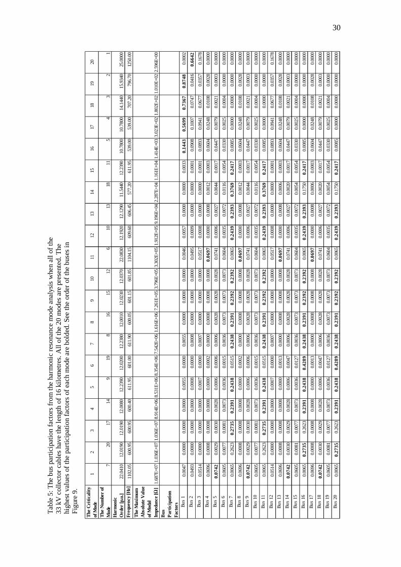
Since the 33 kV collector cables have significant shunt capacitance per unit of length, it is presumable that the length of the cables would have strong effect on resonance points of a network. This section studies the issue. This section shows the results of the modal analysis and the frequency scan in cases where all 33 kV collector cables have the lengths of 16 kilometres (two times the length that they had in Section 4.2) and 32 kilometres (four times the length that they had in Section 4.3), consequently. The cables are modelled as lumped -models. The other parts of the network remain unchanged. The results of the modal analysis are presented in Figures 12 (the case of 16 kilometres) and 15 (the case of 32 kilometres). Furthermore, the bus participation factors can be found in Tables 5 (the case of 16 kilometres) and 6 (the case of 32 kilometres). The results of the frequency scan are presented in Figures 13, 14 and 16. After these studies the parameters of the 33 kV cables in the branches 1 and 3 are changed to correspond to the lengths of 16 kilometres and 32 kilometres (see the branches in Figures 8 and 9). The results of the studies are presented in Figures 17–20.
Figure 12: The curves of the two most critical modes. The 33 kV collector cables have the length of 16 kilometres. The bus participation factors can be found in Table 5. The value of X refers to the harmonic order (the horizontal axis) and the value of Y refers to the absolute value of the modal impedance (the vertical axis).
30
The
Cri
tical
ity
of M
ode
12
34
56
78
910
1112
1314
1516
1718
1920
The
Num
ber o
f M
ode
720
1714
919
816
1512
610
1318
115
43
21
Har
mon
ic
Ord
er [p
.u.]
22.0
410
12.0
190
12.0
190
12.0
080
12.2
390
12.0
200
12.2
380
12.00
1012
.0230
12.03
7022
.083
012
.192
012
.129
011
.544
012
.239
010
.780
010
.780
014
.144
015
.934
025
.000
0Fr
eque
ncy
[Hz]
1102
.05
600.
9560
0.95
600.
4061
1.95
601.
0061
1.90
600.
0560
1.15
601.8
511
04.1
560
9.60
606.
4557
7.20
611.
9553
9.00
539.
0070
7.20
796.
7012
50.0
0Th
e M
axim
um
Abs
olut
e V
alue
of
Mod
al
Impe
danc
e [
]1.
687E
+07
1.03
6E+0
71.
036E
+07
8.91
4E+0
68.
531E
+06
8.35
4E+0
67.
542E
+06
1.61
6E+0
67.2
61E+
053.7
96E+
053.3
02E+
051.
912E
+05
9.19
6E+0
42.
287E
+04
1.16
1E+0
41.
414E
+03
3.02
3E+0
21.
802E
+02
1.01
0E+0
22.
596E
+00
Bus
Pa
rtic
ipat
ion
Fact
ors Bu
s 1
0.00
470.
0000
0.00
000.
0000
0.00
550.0
000
0.005
50.0
000
0.00
000.
0000
0.00
460.
0057
0.00
000.
0000
0.00
330.
1443
0.56
990.
7367
0.87
480.
0002
Bus
20.
0493
0.00
000.
0000
0.00
000.
0008
0.000
00.0
008
0.000
00.
0000
0.00
000.
0495
0.00
090.
0000
0.00
000.
0001
0.09
080.
1007
0.07
470.
0416
0.66
42Bu
s 3
0.05
140.
0000
0.00
000.
0000
0.00
070.0
000
0.000
70.0
000
0.00
000.
0000
0.05
170.
0008
0.00
000.
0000
0.00
010.
0893
0.09
410.
0677
0.03
570.
1678
Bus
40.
0696
0.00
080.
0008
0.00
080.
0000
0.000
20.0
000
0.000
80.
0008
0.00
080.
0697
0.00
000.
0008
0.00
120.
0003
0.06
040.
0248
0.01
080.
0028
0.00
00Bu
s 5
0.07
420.
0029
0.00
300.
0028
0.00
060.0
006
0.000
60.0
028
0.00
280.
0028
0.07
410.
0006
0.00
270.
0044
0.00
170.
0447
0.00
790.
0021
0.00
030.
0000
Bus
60.
0605
0.00
770.
0081
0.00
730.
0036
0.001
50.0
036
0.007
30.
0073
0.00
730.
0604
0.00
350.
0072
0.01
160.
0054
0.03
300.
0025
0.00
040.
0000
0.00
00Bu
s 7
0.00
650.
2623
0.27
350.
2391
0.24
380.0
515
0.24
380.
2391
0.23
920.
2392
0.00
650.
2439
0.23
930.
3769
0.24
170.
0085
0.00
000.
0000
0.00
000.
0000
Bus
80.
0696
0.00
080.
0008
0.00
080.
0000
0.000
20.0
000
0.000
80.
0008
0.00
080.
0697
0.00
000.
0008
0.00
120.
0003
0.06
040.
0248
0.01
080.
0028
0.00
00Bu
s 9
0.07
420.
0029
0.00
300.
0028
0.00
060.0
006
0.000
60.0
028
0.00
280.
0028
0.07
410.
0006
0.00
270.
0044
0.00
170.
0447
0.00
790.
0021
0.00
030.
0000
Bus
100.
0605
0.00
770.
0081
0.00
730.
0036
0.001
50.0
036
0.007
30.
0073
0.00
730.
0604
0.00
350.
0072
0.01
160.
0054
0.03
300.
0025
0.00
040.
0000
0.00
00Bu
s 11
0.00
650.
2623
0.27
350.
2391
0.24
380.0
515
0.24
380.
2391
0.23
920.
2392
0.00
650.
2439
0.23
930.
3769
0.24
170.
0085
0.00
000.
0000
0.00
000.
0000
Bus
120.
0514
0.00
000.
0000
0.00
000.
0007
0.000
00.0
007
0.000
00.
0000
0.00
000.
0517
0.00
080.
0000
0.00
000.
0001
0.08
930.
0941
0.06
770.
0357
0.16
78Bu
s 13
0.06
960.
0008
0.00
080.
0008
0.00
000.0
013
0.000
00.0
008
0.00
080.
0008
0.06
970.
0000
0.00
080.
0006
0.00
030.
0604
0.02
480.
0108
0.00
280.
0000
Bus
140.
0742
0.00
300.
0029
0.00
280.
0006
0.004
70.0
006
0.002
80.
0028
0.00
280.
0741
0.00
060.
0027
0.00
200.
0017
0.04
470.
0079
0.00
210.
0003
0.00
00Bu
s 15
0.06
050.
0081
0.00
770.
0073
0.00
360.0
127
0.003
60.0
073
0.00
730.
0073
0.06
040.
0035
0.00
720.
0054
0.00
540.
0330
0.00
250.
0004
0.00
000.
0000
Bus
160.
0065
0.27
350.
2623
0.23
910.
2438
0.42
890.
2438
0.23
910.
2392
0.23
920.
0065
0.24
390.
2393
0.17
500.
2417
0.00
850.
0000
0.00
000.
0000
0.00
00Bu
s 17
0.06
960.
0008
0.00
080.
0008
0.00
000.0
013
0.000
00.0
008
0.00
080.
0008
0.06
970.
0000
0.00
080.
0006
0.00
030.
0604
0.02
480.
0108
0.00
280.
0000
Bus
180.
0742
0.00
300.
0029
0.00
280.
0006
0.004
70.0
006
0.002
80.
0028
0.00
280.
0741
0.00
060.
0027
0.00
200.
0017
0.04
470.
0079
0.00
210.
0003
0.00
00Bu
s 19
0.06
050.
0081
0.00
770.
0073
0.00
360.0
127
0.003
60.0
073
0.00
730.
0073
0.06
040.
0035
0.00
720.
0054
0.00
540.
0330
0.00
250.
0004
0.00
000.
0000
Bus
200.
0065
0.27
350.
2623
0.23
910.
2438
0.42
890.
2438
0.23
910.
2392
0.23
920.
0065
0.24
390.
2393
0.17
500.
2417
0.00
850.
0000
0.00
000.
0000
0.00
00
Tabl
e 5:
The
bus
par
ticip
atio
n fa
ctor
s fro
m th
e ha
rmon
ic re
sona
nce
mod
e an
alys
is w
hen
all o
f the
33
kV
col
lect
or c
able
s hav
e th
e le
ngth
of 1
6 ki
lom
etre
s. A
ll of
the
20 m
odes
are
pre
sent
ed. T
he
high
est v
alue
s of
the
parti
cipa
tion
fact
ors
of e
ach
mod
e ar
e bo
lded
. See
the
orde
r of t
he b
uses
in
Figu
re 9
.

31
Figure 13: The frequency scan results seen at buses 1–6 when the collector cables have the length of 16 kilometres. The impedance at bus 7 is in its own figure. See the order of the buses in Figure 9.
Figure 14: The impedance of the frequency scan seen at bus 7 in cases when the collector cables have the length of 16 kilometres. See the order of the buses in Figure 9.
12.0 p.u.,620610
0
100000
200000
300000
400000
500000
600000
700000
0 1 2 3 4 5 6 7 8 9 10111213141516171819202122232425
Impe
danc
e (a
bs) [
]
Harmonic Order [p.u.]
Bus 7
22 p.u., 25208
8.2 p.u., 9317
12.0 p.u., 18832
0
5000
10000
15000
20000
25000
30000
0 1 2 3 4 5 6 7 8 9 10111213141516171819202122232425
Impe
danc
e (a
bs) [
]
Harmonic Order [p.u.]
Bus 1Bus 2Bus 3Bus 4Bus 5Bus 6

32
Figure 15: All of the 33 kV collector cables have the length of 32 kilometres. The bus participation factors can be found in Table 6. The value of X refers to the harmonic order (the horizontal axis) and the value of Y refers to the absolute value of the modal impedance (the vertical axis).

33
The
Cri
tical
ity
of M
ode
12
34
56
78
910
1112
1314
1516
1718
1920
The
Num
ber
of
Mod
e6
719
208
1213
149
1517
1610
1118
54
32
1Ha
rmon
ic
Ord
er [p
.u.]
7.873
07.8
740
11.7
650
11.76
5012
.0600
11.75
1011
.7520
11.7
500
12.0
650
11.7
590
11.7
740
11.7
620
11.9
100
13.3
910
12.0
600
10.1
370
10.1
370
13.6
230
14.8
270
25.0
000
Freq
uenc
y [H
z]39
3.65
393.
758
8.25
588.
2560
358
7.55
587.
658
7.5
603.2
558
7.95
588.7
588.1
595.5
669.
5560
350
6.85
506.
8568
1.15
741.
3512
50Th
e M
axim
um
Abso
lute
Val
ue
of M
odal
Im
peda
nce
[]
1.41
1E+0
78.
287E
+06
4.62
7E+0
64.
627E
+06
4.44
2E+0
64.
219E
+06
4.190
E+06
3.752
E+06
1.632
E+06
1.415
E+06
1.24
1E+0
61.
041E
+06
5.80
2E+0
47.
468E
+03
6.25
1E+0
31.
895E
+03
1.27
8E+0
32.
220E
+02
1.38
8E+0
22.
596E
+00
Bus
Part
icip
atio
n Fa
ctor
s Bus 1
0.023
30.0
233
0.000
00.0
000
0.006
30.
0000
0.00
000.
0000
0.00
620.
0000
0.00
000.
0000
0.00
680.
0031
0.00
000.
0954
0.14
430.
6523
0.79
630.
0002
Bus 2
0.041
30.0
414
0.000
00.0
000
0.001
20.
0000
0.00
000.
0000
0.00
120.
0000
0.00
000.
0000
0.00
150.
0000
0.00
000.
0816
0.09
610.
0896
0.06
100.
6642
Bus 3
0.041
70.0
418
0.000
00.0
000
0.001
10.
0000
0.00
000.
0000
0.00
110.
0000
0.00
000.
0000
0.00
140.
0000
0.00
000.
0810
0.09
460.
0828
0.05
430.
1678
Bus 4
0.047
20.0
472
0.001
40.0
003
0.000
00.
0009
0.00
090.
0009
0.00
000.
0009
0.00
170.
0009
0.00
010.
0006
0.02
680.
0664
0.06
820.
0203
0.00
800.
0000
Bus 5
0.053
00.0
530
0.010
80.0
020
0.002
20.
0066
0.00
660.
0066
0.00
220.
0066
0.01
280.
0066
0.00
180.
0050
0.13
900.
0471
0.03
970.
0023
0.00
050.
0000
Bus 6
0.053
50.0
535
0.020
40.0
038
0.006
30.
0124
0.01
240.
0124
0.00
630.
0124
0.02
410.
0123
0.00
580.
0097
0.13
070.
0377
0.02
850.
0005
0.00
010.
0000
Bus 7
0.05
930.
0593
0.39
030.0
718
0.23
910.
2301
0.23
010.
2301
0.23
910.
2301
0.46
080.
2301
0.23
960.
2339
0.00
490.
0140
0.00
620.
0000
0.00
000.
0000
Bus 8
0.047
20.0
472
0.001
40.0
003
0.000
00.
0009
0.00
090.
0009
0.00
000.
0009
0.00
170.
0009
0.00
010.
0006
0.02
680.
0664
0.06
820.
0203
0.00
800.
0000
Bus 9
0.053
00.0
530
0.010
80.0
020
0.002
20.
0066
0.00
660.
0066
0.00
220.
0066
0.01
280.
0066
0.00
180.
0050
0.13
900.
0471
0.03
970.
0023
0.00
050.
0000
Bus 1
00.0
535
0.053
50.0
204
0.003
80.0
063
0.01
240.
0124
0.01
240.
0063
0.01
240.
0241
0.01
230.
0058
0.00
970.
1307
0.03
770.
0285
0.00
050.
0001
0.00
00Bu
s 11
0.05
930.
0593
0.39
030.0
718
0.23
910.
2301
0.23
010.
2301
0.23
910.
2301
0.46
080.
2301
0.23
960.
2339
0.00
490.
0140
0.00
620.
0000
0.00
000.
0000
Bus 1
20.0
417
0.041
80.0
000
0.000
00.0
011
0.00
000.
0000
0.00
000.
0011
0.00
000.
0000
0.00
000.
0014
0.00
000.
0000
0.08
100.
0946
0.08
280.
0543
0.16
78Bu
s 13
0.047
20.0
472
0.000
30.0
014
0.000
00.
0009
0.00
090.
0009
0.00
000.
0009
0.00
000.
0009
0.00
010.
0006
0.01
770.
0664
0.06
820.
0203
0.00
800.
0000
Bus 1
40.0
530
0.053
00.0
020
0.010
80.0
022
0.00
660.
0066
0.00
660.
0022
0.00
660.
0003
0.00
660.
0018
0.00
500.
0919
0.04
710.
0397
0.00
230.
0005
0.00
00Bu
s 15
0.053
50.0
535
0.003
80.0
204
0.006
30.
0124
0.01
240.
0124
0.00
630.
0124
0.00
060.
0123
0.00
580.
0097
0.08
640.
0377
0.02
850.
0005
0.00
010.
0000
Bus 1
60.
0593
0.05
930.0
718
0.39
030.
2391
0.23
010.
2301
0.23
010.
2391
0.23
010.
0112
0.23
010.
2396
0.23
390.
0032
0.01
400.
0062
0.00
000.
0000
0.00
00Bu
s 17
0.047
20.0
472
0.000
30.0
014
0.000
00.
0009
0.00
090.
0009
0.00
000.
0009
0.00
000.
0009
0.00
010.
0006
0.01
770.
0664
0.06
820.
0203
0.00
800.
0000
Bus 1
80.0
530
0.053
00.0
020
0.010
80.0
022
0.00
660.
0066
0.00
660.
0022
0.00
660.
0003
0.00
660.
0018
0.00
500.
0919
0.04
710.
0397
0.00
230.
0005
0.00
00Bu
s 19
0.053
50.0
535
0.003
80.0
204
0.006
30.
0124
0.01
240.
0124
0.00
630.
0124
0.00
060.
0123
0.00
580.
0097
0.08
640.
0377
0.02
850.
0005
0.00
010.
0000
Bus 2
00.
0593
0.05
930.0
718
0.39
030.
2391
0.23
010.
2301
0.23
010.
2391
0.23
010.
0112
0.23
010.
2396
0.23
390.
0032
0.01
400.
0062
0.00
000.
0000
0.00
00
Tabl
e 6:
The
bus
par
ticip
atio
n fa
ctor
s fro
m th
e ha
rmon
ic re
sona
nce
mod
e an
alys
is w
hen
all o
f th
e 33
kV
col
lect
or c
able
s ha
ve th
e le
ngth
of 3
2 ki
lom
etre
s. A
ll of
the
20 m
odes
are
pr
esen
ted.
The
hig
hest
val
ues
of th
e pa
rtici
patio
n fa
ctor
s of e
ach
mod
e ar
e bo
lded
. See
the
orde
r of t
he b
uses
in F
igur
e 9.

34
Figure 16: The frequency scan results seen from the buses 1 to 7 in the case where all of 33 kV collector cables have the length of 32 kilometres. See the order of the buses in Figure 9. Now, two different cases are studied. In the first case the parameters of the 33 kV cables in the branches 1 and 3 are changed to correspond to the lengths of 16 kilometres (see the branches in Figures 8 and 9). In the second case the same cables have the length of 32 kilometres. In both of the cases the cable lengths of the branches 2 and 4 are 8 kilometres. The results of the first case are in Figures 17 (modal analysis) and 18 (frequency scan). The results of the second case are in Figures 19 (modal analysis) and 20 (frequency scan). The participation factors are in Tables 1 (the first case) and 2 (the second case) in Appendix A in order to make the reading of the thesis easier.
19.4 p.u.,44020
7.9 p.u., 11798
11.8 p.u., 195574
0
50000
100000
150000
200000
250000
0 1 2 3 4 5 6 7 8 9 10111213141516171819202122232425
Impe
danc
e (a
bs) [
]
Harmonic Order [p.u.]
Bus 1Bus 2Bus 3Bus 4Bus 5Bus 6Bus 7
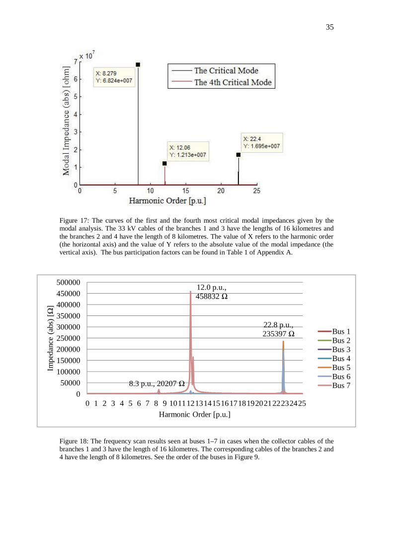
35
Figure 17: The curves of the first and the fourth most critical modal impedances given by the modal analysis. The 33 kV cables of the branches 1 and 3 have the lengths of 16 kilometres and the branches 2 and 4 have the length of 8 kilometres. The value of X refers to the harmonic order (the horizontal axis) and the value of Y refers to the absolute value of the modal impedance (the vertical axis). The bus participation factors can be found in Table 1 of Appendix A.
Figure 18: The frequency scan results seen at buses 1–7 in cases when the collector cables of the branches 1 and 3 have the length of 16 kilometres. The corresponding cables of the branches 2 and 4 have the length of 8 kilometres. See the order of the buses in Figure 9.
22.8 p.u., 235397
8.3 p.u., 20207
12.0 p.u.,458832
050000
100000150000200000250000300000350000400000450000500000
0 1 2 3 4 5 6 7 8 9 10111213141516171819202122232425
Impe
danc
e (a
bs) [
]
Harmonic Order [p.u.]
Bus 1Bus 2Bus 3Bus 4Bus 5Bus 6Bus 7
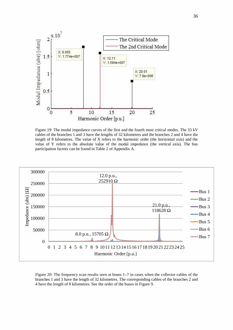
36
Figure 19: The modal impedance curves of the first and the fourth most critical modes. The 33 kV cables of the branches 1 and 3 have the lengths of 32 kilometres and the branches 2 and 4 have the length of 8 kilometres. The value of X refers to the harmonic order (the horizontal axis) and the value of Y refers to the absolute value of the modal impedance (the vertical axis). The bus participation factors can be found in Table 2 of Appendix A.
Figure 20: The frequency scan results seen at buses 1–7 in cases when the collector cables of the branches 1 and 3 have the length of 32 kilometres. The corresponding cables of the branches 2 and 4 have the length of 8 kilometres. See the order of the buses in Figure 9.
21.0 p.u.,118628
8.0 p.u., 15705
12.0 p.u.,252910
0
50000
100000
150000
200000
250000
300000
0 1 2 3 4 5 6 7 8 9 1011 12 13 1415 16 17 1819 20 21 2223 24 25
Impe
danc
e (a
bs) [
]
Harmonic Order [p.u.]
Bus 1Bus 2Bus 3Bus 4Bus 5Bus 6Bus 7

37
4.4 The Effect of Transmission Cable Length on the Resonance
Points
This section addresses the effect of the change of the length parameters of 150 kV cables on the resonances. 150 kV transmission cables are situated between buses 2 and 3, and 2–12 (see Figure 9). Longer cables, not 58 km but 116 km in the first case and 174 km in the second case. The parameters of 33 kV collector cables are maintained to correspond to the length of 8 kilometres in both cases. The modal impedance curves of the critical, second critical and sixth most critical modes are shown in Figures 21 and 23. The corresponding frequency-impedance curves of the frequency scan are shown in Figures 22 and 24. The bus participation factors of both of the cases are presented in Tables 1 and 2 (respectively) in Appendix B in order to make the reading of this thesis easier.
Figure 21: Three selected modes of the modal analysis. 150 kV transmission cables are 116 kilometres long (double their length in comparison with the case in Section 4.2). The corresponding bus participation factors can be found in Table 1 of Appendix B. The value of X refers to the harmonic order (the horizontal axis) and the value of Y refers to the absolute value of the modal impedance (the vertical axis).

38
Figure 22: The results of the frequency scan, when both 150kV cables have the length of 116 kilometres. See the order of the buses in Figure 9.
Figure 23: The first and the second most critical modes in the situation, where the electrical parameters of 150 kV cables are changed to correspond to the length of 174 kilometres. The corresponding bus participation factors can be found in Table 2 of Appendix B. The value of X refers to the harmonic order (the horizontal axis) and the value of Y refers to the absolute value of the modal impedance (the vertical axis).
19.2 p.u., 9063
7.7 p.u., 151505
12.1 p.u., 628149
0100000200000300000400000500000600000700000
0 1 2 3 4 5 6 7 8 9 10111213141516171819202122232425
Impe
danc
e (a
bs) [
]
Harmonic Order [p.u.]
Bus 1Bus 2Bus 3Bus 4Bus 5Bus 6Bus 7

39
Figure 24: The results of the frequency scan, when the electrical parameters of 150 kV cables are changed to correspond to the length of 174 kilometres. See the order of the buses in Figure 9.
4.5 Passive Filters at the Critical Buses
In this section, second-order shunt passive filters are connected to buses 7, 11, 16, and 20 (see Figure 9) to damp the resonance peaks. One filter is connected to each bus, therefore, totally four filters are installed. The filter is a typical second-order shunt filter with a resistance and an inductance in parallel with each other and a capacitance connected in series with them. The configuration of the passive filter with the values of the resistance (R), the inductance (L) and the capacitance (C) are shown in Figure 25.
7.1 p.u., 11353
12.1 p.u.,295738
17.4 p.u., 4298 0
50000
100000
150000
200000
250000
300000
350000
0 1 2 3 4 5 6 7 8 9 10111213141516171819202122232425
Impe
danc
e (a
bs) [
]
Harmonic Order [p.u.]
Bus 1Bus 2Bus 3Bus 4Bus 5Bus 6Bus 7

40
Figure 25: The shunt passive filter placed at buses 7, 11, 16 and 20. R is the resistance, L is the inductance and C is the capacitance of the passive filter. See the order of the buses in Figure 9. Three stripes signify a three phase current and voltage. Passive filters are usually designed for damping even rather than inter harmonics. Following this practice, the filters are dimensioned for the 12th harmonic (600 Hz) because that is the nearest even harmonic to the critical modes that are around 12.12 per unit (606 Hz). According to the bus participation factors (Table 4) the bus participation factors at buses 7, 11, 16 and 20 are the best locations to place the filters, so they are placed in parallel with the LCL filter capacitances. The curves of the modal impedances and the result of the frequency scan are shown in Figures 26 (modal impedance curves) and 27 (frequency-impedance curves of the frequency scan). The frequency scan is calculated at all buses 1–7 (see Figure 9). Table 7 shows the bus participation factors.

41
Figure 26: Three selected mode curves, when the passive filters are placed at buses 7, 11, 16 and 20. The value of X refers to the harmonic order (the horizontal axis) and the value of Y refers to the absolute value of the modal impedance (the vertical axis). See the order of the buses in Figure 9.
Figure 27: The impedances measured with the frequency scan at buses 1–7. See the order of the buses in Figure 9.
Impedance (abs) [ ]
9.1 p.u., 7473
23.5 p.u., 26843
2.3 p.u., 10766
0
5000
10000
15000
20000
25000
30000
35000
40000
0 1 2 3 4 5 6 7 8 9 10 11 12 13 14 15 16 17 18 19 20 21 22 23 24 25Harmonic Order [p.u.]
Bus 1
Bus 2
Bus 3
Bus 4
Bus 5
Bus 6
Bus 7
Impedance (abs) [ ]

42
The
Criti
calit
y of
Mod
e1
23
45
67
89
1011
1213
1415
1617
1819
20
The
Num
ber o
f M
ode
56
73
98
1014
1516
2019
1712
1113
184
21
Har
mon
ic
Ord
er [p
.u.]
23.5
410
23.5
400
23.5
250
23.05
002.
1460
2.14
82.
188
2.27
12.
272.2
672.
273
2.27
32.
275
24.9
9424
.993
24.9
9124
.991
12.58
616
.161
25Fr
eque
ncy
[Hz]
1177
.05
1177
1176
.25
1152
.510
7.3
107.4
109.
411
3.55
113.
511
3.35
113.6
511
3.65
113.
7512
49.7
1249
.65
1249
.55
1249
.55
629.3
808.
0512
50Th
e M
axim
um
Abs
olut
e V
alue
of
Mod
al
Impe
danc
e [
]2.
050E
+06
2.04
5E+0
69.
038E
+05
3.20
1E+0
43.8
91E+
033.
891E
+03
3.65
3E+0
32.
902E
+03
2.90
2E+0
32.
900E
+03
2.896
E+03
2.89
6E+0
32.
896E
+03
1.35
4E+0
31.
354E
+03
1.35
3E+0
31.2
72E+
034.1
82E+
029.
569E
+01
2.59
6E+0
0B
us
Part
icip
atio
n Fa
ctor
s Bus
10.
0038
0.00
380.0
038
0.00
410.
0017
0.00
170.
0016
0.00
000.
0000
0.000
00.
0000
0.00
000.
0000
0.00
000.
0000
0.000
00.
0000
0.47
220.
8879
0.00
02Bu
s 2
0.05
980.
0598
0.059
70.
0569
0.00
660.
0066
0.00
620.
0000
0.00
000.0
000
0.00
000.
0000
0.00
000.
0000
0.00
000.0
000
0.00
000.
1062
0.03
820.
6642
Bus
30.
0620
0.06
200.0
619
0.05
910.
0068
0.00
670.
0063
0.00
000.
0000
0.000
00.
0000
0.00
000.
0000
0.00
010.
0001
0.000
10.
0000
0.10
030.
0324
0.16
78Bu
s 4
0.07
090.
0709
0.070
90.
0706
0.01
030.
0103
0.00
970.
0007
0.00
070.0
007
0.00
010.
0014
0.00
080.
0453
0.04
530.0
453
0.09
170.
0300
0.00
180.
0000
Bus
50.
0712
0.07
120.
0712
0.07
180.
0122
0.01
220.
0116
0.00
150.
0015
0.001
50.
0003
0.00
300.
0016
0.07
760.
0776
0.077
60.
1620
0.01
800.
0004
0.00
00Bu
s 6
0.06
100.
0610
0.061
00.
0628
0.01
850.
0185
0.01
770.
0053
0.00
530.0
053
0.00
110.
0108
0.00
600.
1271
0.12
710.
1271
0.27
470.
0073
0.00
000.
0000
Bus
70.
0000
0.00
000.0
000
0.00
000.
2041
0.20
420.
2066
0.24
250.
2425
0.24
250.
0535
0.51
250.
2832
0.00
000.
0000
0.000
00.
0000
0.00
000.
0000
0.00
00Bu
s 8
0.07
090.
0709
0.070
90.
0706
0.01
030.
0103
0.00
970.
0007
0.00
070.0
007
0.00
010.
0014
0.00
080.
0453
0.04
530.0
453
0.09
170.
0300
0.00
180.
0000
Bus
90.
0712
0.07
120.
0712
0.07
180.
0122
0.01
220.
0116
0.00
150.
0015
0.001
50.
0003
0.00
300.
0016
0.07
760.
0776
0.077
60.
1620
0.01
800.
0004
0.00
00Bu
s 10
0.06
100.
0610
0.061
00.
0628
0.01
850.
0185
0.01
770.
0053
0.00
530.0
053
0.00
110.
0108
0.00
600.
1271
0.12
710.
1271
0.27
470.
0073
0.00
000.
0000
Bus
110.
0000
0.00
000.0
000
0.00
000.
2041
0.20
420.
2066
0.24
250.
2425
0.24
250.
0535
0.51
250.
2832
0.00
000.
0000
0.000
00.
0000
0.00
000.
0000
0.00
00Bu
s 12
0.06
200.
0620
0.061
90.
0591
0.00
680.
0067
0.00
630.
0000
0.00
000.0
000
0.00
000.
0000
0.00
000.
0001
0.00
010.0
001
0.00
000.
1003
0.03
240.
1678
Bus
130.
0709
0.07
090.0
709
0.07
060.
0103
0.01
030.
0097
0.00
070.
0007
0.000
70.
0014
0.00
010.
0006
0.04
530.
0453
0.045
30.
0104
0.03
000.
0018
0.00
00Bu
s 14
0.07
120.
0712
0.07
120.
0718
0.01
220.
0122
0.01
160.
0015
0.00
150.0
015
0.00
300.
0003
0.00
120.
0776
0.07
760.0
776
0.01
840.
0180
0.00
040.
0000
Bus
150.
0610
0.06
100.0
610
0.06
280.
0185
0.01
850.
0177
0.00
530.
0053
0.005
30.
0108
0.00
110.
0045
0.12
710.
1271
0.12
710.
0312
0.00
730.
0000
0.00
00Bu
s 16
0.00
000.
0000
0.000
00.
0000
0.20
410.
2042
0.20
660.
2425
0.24
250.
2425
0.51
250.
0535
0.21
270.
0000
0.00
000.0
000
0.00
000.
0000
0.00
000.
0000
Bus
170.
0709
0.07
090.0
709
0.07
060.
0103
0.01
030.
0097
0.00
070.
0007
0.000
70.
0014
0.00
010.
0006
0.04
530.
0453
0.045
30.
0104
0.03
000.
0018
0.00
00Bu
s 18
0.07
120.
0712
0.07
120.
0718
0.01
220.
0122
0.01
160.
0015
0.00
150.0
015
0.00
300.
0003
0.00
120.
0776
0.07
760.0
776
0.01
840.
0180
0.00
040.
0000
Bus
190.
0610
0.06
100.0
610
0.06
280.
0185
0.01
850.
0177
0.00
530.
0053
0.005
30.
0108
0.00
110.
0045
0.12
710.
1271
0.12
710.
0312
0.00
730.
0000
0.00
00Bu
s 20
0.00
000.
0000
0.000
00.
0000
0.20
410.
2042
0.20
660.
2425
0.24
250.
2425
0.51
250.
0535
0.21
270.
0000
0.00
000.0
000
0.00
000.
0000
0.00
000.
0000
Tabl
e 7:
Bus
par
ticip
atio
n fa
ctor
s of
the
mod
es fr
om th
e 8th
unt
il th
e 14
th,
whe
n th
e pa
ssiv
e fil
ters
are
loc
ated
at
buse
s 7,
11,
16
and
20.
The
parti
cipa
tion
fact
ors
with
the
high
est v
alue
s ar
e bo
lded
. See
the
ord
er o
f th
e bu
ses i
n Fi
gure
9.

43
4.6 Hybrid Filters at the Critical Buses
Instead of passive filters, simple hybrid filters are placed at buses 7, 11, 16 and 20 (one filter at each bus). The buses are the same where the passive filters were in Section 4.5 (see Figure 9). A hybrid filter is like a passive filter equipped with control and a controlled voltage source. The passive components (R, L and C) of the hybrid filters are the same as for the passive filters in Section 4.5 (see Figure 25). Figure 28 shows a scheme of the hybrid filter. More detailed explanation of the hybrid filter can be found in [91].
Figure 28: Hybrid filter connected to the buses 7, 11, 16 and 20. See the order of the buses in Figure 9. Three stripes signify a three phase current and voltage. The idea of the control is that the filter damps all the other frequencies except the fundamental one (50 Hz). For the fundamental frequency the filter appears as passive filter as shown in Figure 29. Because the filter is tuned to the harmonic frequency, it does not have any effect on the fundamental frequency. [91]
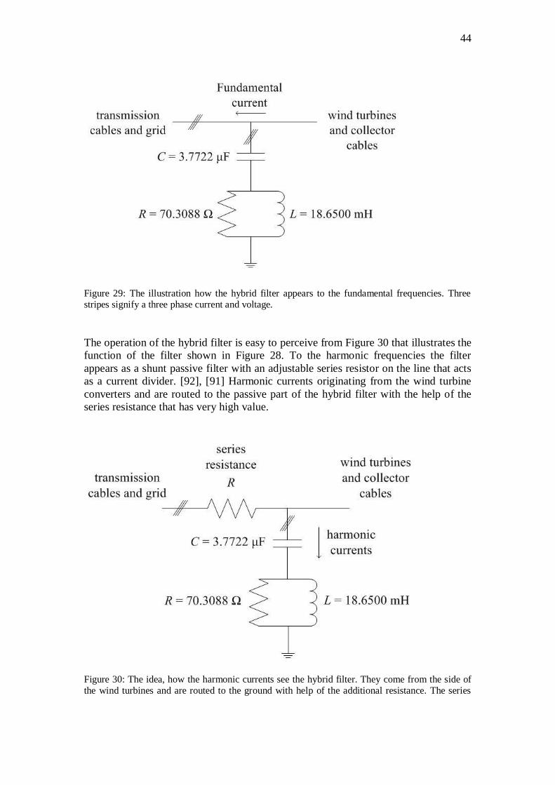
44
Figure 29: The illustration how the hybrid filter appears to the fundamental frequencies. Three stripes signify a three phase current and voltage. The operation of the hybrid filter is easy to perceive from Figure 30 that illustrates the function of the filter shown in Figure 28. To the harmonic frequencies the filter appears as a shunt passive filter with an adjustable series resistor on the line that acts as a current divider. [92], [91] Harmonic currents originating from the wind turbine converters and are routed to the passive part of the hybrid filter with the help of the series resistance that has very high value.
Figure 30: The idea, how the harmonic currents see the hybrid filter. They come from the side of the wind turbines and are routed to the ground with help of the additional resistance. The series

45
resistance has an extremely high value in order to route as many harmonic current to the filter as possible. Three stripes signify a three phase current and voltage. Figure 31 shows the behaviour of the resistance as a function of frequency. The resistance approaches zero at the fundamental frequency.
Figure 31: The behaviour of the additional resistance as a function of frequency. Note that frequency is in per units. The greater is the value of the resistance the more harmonic current is routed to the filter. In theory, if the resistance was infinitely large, all the harmonic currents would go the passive part of the filter and not continue their way to the transmission grid. Figure 32 shows the modal impedance curves of the three most critical modes when the hybrid filters are placed in the grid. Figure 33 shows the corresponding results of the frequency scan. The bus participation factors of the case are shown in Table 8.

46
Figure 32: The three most critical modes when the hybrid filters are placed to buses 7, 11, 16 and 20. The value of X refers to the harmonic order (the horizontal axis) and the value of Y refers to the absolute value of the modal impedance (the vertical axis). Table 8 shows the bus participation factors. See the order of the buses in Figure 9.
Figure 33: The results of the frequency scan in the case, where the hybrid filters are placed at buses 7, 11, 16 and 20. The frequency scan is calculated at buses 1–7. See the order of the buses in Figure 9.
23.5 p.u.,21989
9.1 p.u., 5306
0
5000
10000
15000
20000
25000
0 1 2 3 4 5 6 7 8 9 10 11 12 13 14 15 16 17 18 19 20 21 22 23 24 25Harmonic Order [p.u.]
Bus 1Bus 2Bus 3Bus 4Bus 5Bus 6Bus 7
Impedance (abs) [ ]

47
The
Cri
tical
ity
of M
ode
12
34
56
78
910
1112
1314
1516
1718
1920
The
Num
ber
of
Mod
e4
67
35
98
1513
1417
1820
1912
1610
112
1Ha
rmon
ic
Ord
er [p
.u.]
23.5
550
23.5
420
23.5
970
23.4
100
9.11
6010
.072
1.68
21.
651.
648
1.63
31.
651.
651.
633
1.63
31.
621.
575
1.57
524
.941
12.6
9425
Freq
uenc
y [H
z]11
77.7
511
77.1
1179
.85
1170
.545
5.8
503.
684
.182
.582
.481
.65
82.5
82.5
81.6
581
.65
81.0
078
.75
78.7
512
47.0
563
4.7
1250
The
Max
imum
Ab
solu
te V
alue
of
Mod
al
Impe
danc
e [
]1.
091E
+05
1.08
7E+0
51.
047E
+05
7.69
8E+0
44.
705E
+04
3.23
6E+0
32.
636E
+03
2.39
4E+0
32.
394E
+03
2.39
2E+0
32.
391E
+03
2.39
1E+0
32.
389E
+03
2.38
9E+0
32.
389E
+03
2.36
2E+0
32.
206E
+03
2.20
3E+0
32.
550E
+02
2.60
8E+0
0Bu
s Pa
rtic
ipat
ion
Fact
ors Bu
s 10.
0037
0.00
370.
0037
0.00
380.
0588
0.10
760.
0003
0.00
000.
0000
0.00
000.
0000
0.00
000.
0000
0.00
000.
0000
0.00
000.
0000
0.00
000.
5404
0.00
02Bu
s 20.
0595
0.05
940.
0598
0.05
860.
0717
0.09
150.
0010
0.00
000.
0000
0.00
000.
0000
0.00
000.
0000
0.00
000.
0000
0.00
000.
0000
0.00
000.
1699
0.67
04Bu
s 30.
0617
0.06
160.
0620
0.06
080.
0718
0.09
070.
0010
0.00
000.
0000
0.00
000.
0000
0.00
000.
0000
0.00
000.
0000
0.00
000.
0000
0.00
000.
1643
0.16
47Bu
s 40.
0715
0.07
150.
0715
0.07
160.
0669
0.07
940.
0535
0.05
530.
0553
0.05
570.
0777
0.04
130.
0080
0.10
430.
0561
0.05
720.
0811
0.08
110.
0061
0.00
00Bu
s 50.
0718
0.07
180.
0717
0.07
210.
0640
0.07
230.
0543
0.05
590.
0559
0.05
630.
0785
0.04
180.
0081
0.10
540.
0567
0.05
780.
0889
0.08
890.
0029
0.00
00Bu
s 60.
0614
0.06
140.
0612
0.06
200.
0546
0.05
720.
0564
0.05
760.
0576
0.05
800.
0809
0.04
300.
0084
0.10
850.
0583
0.05
920.
0867
0.08
670.
0008
0.00
00Bu
s 70.
0000
0.00
000.
0000
0.00
000.
0001
0.00
010.
0875
0.08
270.
0826
0.08
140.
1162
0.06
180.
0117
0.15
220.
0804
0.07
710.
0000
0.00
000.
0000
0.00
00Bu
s 80.
0715
0.07
150.
0715
0.07
160.
0669
0.07
940.
0535
0.05
530.
0553
0.05
570.
0777
0.04
130.
0080
0.10
430.
0561
0.05
720.
0811
0.08
110.
0061
0.00
00Bu
s 90.
0718
0.07
180.
0717
0.07
210.
0640
0.07
230.
0543
0.05
590.
0559
0.05
630.
0785
0.04
180.
0081
0.10
540.
0567
0.05
780.
0889
0.08
890.
0029
0.00
00Bu
s 10
0.06
140.
0614
0.06
120.
0620
0.05
460.
0572
0.05
640.
0576
0.05
760.
0580
0.08
090.
0430
0.00
840.
1085
0.05
830.
0592
0.08
670.
0867
0.00
080.
0000
Bus 1
10.
0000
0.00
000.
0000
0.00
000.
0001
0.00
010.
0875
0.08
270.
0826
0.08
140.
1162
0.06
180.
0117
0.15
220.
0804
0.07
710.
0000
0.00
000.
0000
0.00
00Bu
s 12
0.06
170.
0616
0.06
200.
0608
0.07
180.
0907
0.00
100.
0000
0.00
000.
0000
0.00
000.
0000
0.00
000.
0000
0.00
000.
0000
0.00
000.
0000
0.16
430.
1647
Bus 1
30.
0715
0.07
150.
0715
0.07
160.
0669
0.07
940.
0535
0.05
530.
0553
0.05
570.
0413
0.07
770.
1043
0.00
800.
0561
0.05
720.
0811
0.08
110.
0061
0.00
00Bu
s 14
0.07
180.
0718
0.07
170.
0721
0.06
400.
0723
0.05
430.
0559
0.05
590.
0563
0.04
180.
0785
0.10
540.
0081
0.05
670.
0578
0.08
890.
0889
0.00
290.
0000
Bus 1
50.
0614
0.06
140.
0612
0.06
200.
0546
0.05
720.
0564
0.05
760.
0576
0.05
800.
0430
0.08
090.
1085
0.00
840.
0583
0.05
920.
0867
0.08
670.
0008
0.00
00Bu
s 16
0.00
000.
0000
0.00
000.
0000
0.00
010.
0001
0.08
750.
0827
0.08
260.
0814
0.06
180.
1162
0.15
220.
0117
0.08
040.
0771
0.00
000.
0000
0.00
000.
0000
Bus 1
70.
0715
0.07
150.
0715
0.07
160.
0669
0.07
940.
0535
0.05
530.
0553
0.05
570.
0413
0.07
770.
1043
0.00
800.
0561
0.05
720.
0811
0.08
110.
0061
0.00
00Bu
s 18
0.07
180.
0718
0.07
170.
0721
0.06
400.
0723
0.05
430.
0559
0.05
590.
0563
0.04
180.
0785
0.10
540.
0081
0.05
670.
0578
0.08
890.
0889
0.00
290.
0000
Bus 1
90.
0614
0.06
140.
0612
0.06
200.
0546
0.05
720.
0564
0.05
760.
0576
0.05
800.
0430
0.08
090.
1085
0.00
840.
0583
0.05
920.
0867
0.08
670.
0008
0.00
00Bu
s 20
0.00
000.
0000
0.00
000.
0000
0.00
010.
0001
0.08
750.
0827
0.08
260.
0814
0.06
180.
1162
0.15
220.
0117
0.08
040.
0771
0.00
000.
0000
0.00
000.
0000
Tabl
e 8:
The
bus
par
ticip
atio
n fa
ctor
s whe
n th
e hy
brid
filte
rs a
re p
lace
d at
bus
es 7
, 11,
16
and
20. S
ee th
e or
der o
f the
bus
es in
Fig
ure
9. T
he p
artic
ipat
ion
fact
ors w
ith th
e hi
ghes
t val
ues
of
each
mod
e ar
e bo
lded
.

48
4.7 Harmonic Current and Voltage Analyses
Until this point, some characteristics of the resonances have been studied. In this section, harmonic currents originating from the wind turbine converter are injected in the wind power plant. This section shows what happens when harmonic currents are injected into the grid that is prone to trigger resonances. In addition, the effect of a passive filter on harmonic currents and voltages will be demonstrated. All the harmonic current and voltage analyses are performed by using PSCAD software.
4.7.1 Harmonic Current and Voltage Analysis of the Wind Power Plant
The injected harmonic currents follow the requirements of the German Electricity Association for the harmonic emissions of wind turbine converters [93]. The requirements are presented in Section 2.5. The precise injected harmonic currents are shown in Table 9. The harmonic currents in Table 9 are calculated as explained in Section 2.6 (Equation (10) and Table 2)). The short circuit ratio is 20 and the voltage level is 150 kV. The converters are modelled as harmonic current sources (see Figure 34). The harmonic currents below the 26th order are injected in the simulations at bus 5 (see Figure 34). Triple harmonics are excluded as they are normally eliminated in transformer windings. Current at the fundamental frequency is not injected into the grid, because in this way it is easier to distinguish the effect of passive filtering on current and voltage waveforms. Table 9: Injected harmonic currents that do not exceed the limits of the requirements of the German Electricity Association. The harmonic currents are calculated according to the explanation in Section 2.5.
The limits for the harmonic current emissions of the German Electricity Association cover the combination of a converter and an output filter. In other words, the harmonic currents coming out from a converter can exceed the limits, but the
Harmonic Order Current [A] Harmonic Order Current [A]
2 4.445 17.04 4 2.227 12.15 8 1.1111 7.70 10 0.8913 5.63 12 0.7417 3.26 14 0.6319 2.67 16 0.5623 1.78 18 0.4925 1.48 20 0.44
22 0.4024 0.37

49
harmonic currents have to be under the limits after flowing through the output filter. In this case, the output filter is an LCL filter. According to this the wind turbines and the LCL filters are together placed by the harmonic current sources. In the resonance calculations of the earlier sections of this chapter, the LCL filters have been considered as parts of the network and not as parts of the output filters. In this section, the LCL filters are excluded from the network as they are seen as parts of the converters (current sources). Taking away the LCL filters shifts the resonance frequencies and that is why a new resonance analysis of the wind power plant has to be performed. The removal of the output filters from the model of the wind power plant reduces the number of buses from 20 to 12. The reduced model of the aggregated wind power plant is presented in Figure 34. The components of the network have the same values as in the earlier sections (see Table 3).
Figure 34: The reduced model of the wind power plant for the harmonic current and voltage analyses. Here, the LCL filters are not a part of the network as they belong to the harmonic current sources. The values of the component are in Table 3. Figure 35 shows the curve of the critical mode and Table 10 presents the bus participation factors. In this case only one mode (the critical one) is needed to describe the resonance conditions of the network quite well. This is because, the second critical mode has significantly smaller maximum modal impedance compared with the critical one. This can be confirmed by observing the impedance calculated by

50
the frequency scan in Figure 36. According to Figure 35 the network has two clear resonance points: 8.535 per unit (427 Hz) and 22.610 per unit (1130 Hz). The bus participation factors of Table 10 show (the column of the critical mode) that the major resonance is divided evenly between several buses, and therefore, several filters are required to damp this resonance efficiently.
Figure 35: The impedance curve of the critical mode given by the modal analysis in the case of 12 buses (Figure 34). The same model is used in harmonic current and voltage analysis. The value of X refers to the harmonic order (the horizontal axis) and the value of Y refers to the absolute value of the modal impedance (the vertical axis). The values of the bus participation factors are in Table 10. See the order of the buses in Figure 34.

51
The
Cri
tical
ity
of M
ode
12
34
56
78
910
1112
The
Num
ber
of
Mod
e5
410
87
912
113
26
1H
arm
onic
O
rder
[p.u
.]22
.608
010
.435
025
.000
024
.999
024
.997
024
.988
2524
.988
14.1
4315
.431
2525
Freq
uenc
y [H
z]11
30.4
521.
7512
5012
49.9
512
49.8
512
49.4
1250
1249
.470
7.15
771.
5512
5012
50Th
e M
axim
um
Abs
olut
e V
alue
of
Mod
al
Impe
danc
e [
]
1.36
0E+0
71.
528E
+03
8.57
2E+0
28.
571E
+02
8.57
0E+0
28.
566E
+02
8.12
3E+0
28.
118E
+02
1.80
9E+0
21.
160E
+02
7.57
3E+0
02.
596E
+00
Bus
Pa
rtic
ipat
ion
Fact
ors Bu
s 1
0.00
580.
1303
0.00
000.
0000
0.00
000.
0000
0.00
000.
0000
0.73
330.
8493
0.00
000.
0002
Bus
20.
0713
0.09
810.
0000
0.00
000.
0000
0.00
000.
0000
0.00
000.
0736
0.04
840.
0000
0.66
42Bu
s 3
0.07
420.
0969
0.00
020.
0002
0.00
020.
0002
0.00
000.
0000
0.06
670.
0420
0.49
930.
1678
Bus
40.
0943
0.07
460.
0977
0.09
770.
0977
0.09
770.
0108
0.02
850.
0101
0.00
340.
0004
0.00
00Bu
s 5
0.09
940.
0698
0.15
220.
1522
0.15
220.
1522
0.01
720.
0454
0.00
490.
0011
0.00
000.
0000
Bus
60.
0943
0.07
460.
0977
0.09
770.
0977
0.09
770.
0108
0.02
850.
0101
0.00
340.
0004
0.00
00Bu
s 7
0.09
940.
0698
0.15
220.
1522
0.15
220.
1522
0.01
720.
0454
0.00
490.
0011
0.00
000.
0000
Bus
80.
0742
0.09
690.
0002
0.00
020.
0002
0.00
020.
0000
0.00
000.
0667
0.04
200.
4993
0.16
78Bu
s 9
0.09
430.
0746
0.09
770.
0977
0.09
770.
0977
0.18
270.
1712
0.01
010.
0034
0.00
040.
0000
Bus
100.
0994
0.06
980.
1522
0.15
220.
1522
0.15
220.
2911
0.27
280.
0049
0.00
110.
0000
0.00
00Bu
s 11
0.09
430.
0746
0.09
770.
0977
0.09
770.
0977
0.18
270.
1712
0.01
010.
0034
0.00
040.
0000
Bus
120.
0994
0.06
980.
1522
0.15
220.
1522
0.15
220.
2911
0.27
280.
0049
0.00
110.
0000
0.00
00
Tabl
e 10
: The
par
ticip
atio
n fa
ctor
s of a
ll of
the
mod
es in
the
case
of 1
2 bu
ses.
The
parti
cipa
tion
fact
ors
with
the
high
est v
alue
s of
eac
h m
ode
are
bold
ed. S
ee th
e nu
mbe
ring
of th
e bu
ses i
n Fi
gure
34
.

52
Figure 36: The results of the frequency scan in the reduced network of the wind power plant (see Figure 34). The frequency scan is calculated at buses 1–5. Harmonic currents presented in Table 7 are injected into bus 5. The voltage at the point of grid connection is a nominal value since there is an ideal voltage source connected. Harmonic current and voltage measurements are performed at buses 1, 2 and 4. Figure 37 shows the absolute values of the measured currents divided by the injected currents at all the buses. In the figure it is easy to see the amplification of each harmonic current.
22.6 p.u., 9029 8.5 p.u., 9564
0
2000
4000
6000
8000
10000
12000
14000
16000
18000
0 1 2 3 4 5 6 7 8 9 10 11 12 1314 15 16 17 18 1920 21 22 23 2425
Impe
danc
e (a
bs) [
]
Harmonic Order [p.u.]
Bus 1
Bus 2
Bus 3
Bus 4
Bus 5

53
Figure 37: Measured harmonic currents divided by the injected harmonic currents. The currents are measured at buses 1, 2 and 4. See the order of the buses in Figure 34. Figure 38 shows the voltages at buses 1, 2, 4 and 5. Note, that bus 5 is the injection bus and that the voltage is in per units. The amplification of the voltages (with respect to their value at bus 5) is shown in Figure 39. The figure shows the voltages measured at buses 1, 2 and 4 divided by the voltage at bus 5 (the harmonic current injection). In other words, Figure 39 presents the relative voltage amplification at harmonic frequencies.
0
10
20
30
40
50
60
2 4 5 7 8 10 11 12 13 14 16 17 18 19 20 22 23 24 25
Cur
rent
/ In
ject
ed C
urre
nt [p
.u.]
Harmonic Order [p.u.]
Bus 4Bus 2Bus 1
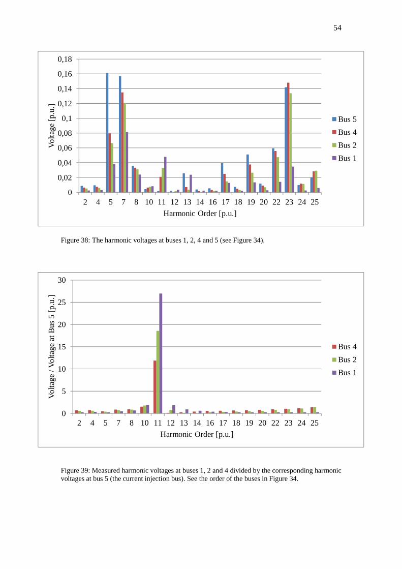
54
Figure 38: The harmonic voltages at buses 1, 2, 4 and 5 (see Figure 34).
Figure 39: Measured harmonic voltages at buses 1, 2 and 4 divided by the corresponding harmonic voltages at bus 5 (the current injection bus). See the order of the buses in Figure 34.
0
5
10
15
20
25
30
2 4 5 7 8 10 11 12 13 14 16 17 18 19 20 22 23 24 25
Volta
ge /
Volta
ge a
t Bus
5 [p
.u.]
Harmonic Order [p.u.]
Bus 4Bus 2Bus 1
0
0,02
0,04
0,06
0,08
0,1
0,12
0,14
0,16
0,18
2 4 5 7 8 10 11 12 13 14 16 17 18 19 20 22 23 24 25
Volta
ge [p
.u.]
Harmonic Order [p.u.]
Bus 5Bus 4Bus 2Bus 1

55
4.7.2 Harmonic Current and Voltage Analysis with Passive Filters In this section the current and voltages analyses are performed, but placing two kinds of passive filters to the network. The other type of filter is designed to damp resonances at the 8th (400 Hz) order and the other type to damp resonances at the 23th (1150 Hz) order. Both of these passive filters are of the same topology as used in the earlier cases (see Figure 25). The values of the components of the passive filters are shown in Table 11. One filter (that is designed for damping resonances at the 8th order) is connected to bus 1. One passive filter (that is designed for damping resonances at the 23rd order) is connected to buses 3 and 8 (one filter to each bus). Totally three passive filters are connected to the network. Table 11: The values of the electrical components of the passive filters. The topology of the filters is the same as in Figure 25. See the order of the buses in Figure 34.
The modal curve of the critical mode is shown in Figure 40 and the bus participation factors are presented in Table 12. Figure 41 presents the impedance curves given by the frequency scan at buses 1–5 (see Figure 34).
Figure 40: The modal impedance curve of the critical mode given by the modal analysis. Passive filters are placed in the network at buses 1 (for damping the 8th order harmonics), 3 (for damping the 23rd order harmonics) and 8 (for damping the 23rd order harmonics). The value of X refers to the harmonic order (the horizontal axis) and the value of Y refers to the absolute value of the modal impedance (the vertical axis). The participation factors are in Table 12. See the order of the buses in Figure 34.
Bus Resistance (R ) Inductance (L ) Capacitance (C ) Harmonic Order Frequency1 210.96 83.90 mH 1.89 F 8 p.u. 400 Hz
3, 8 134.30 18.60 mH 1.03 F 23 p.u. 1150 Hz

56
The
Cri
tical
ity
of M
ode
12
34
56
78
910
1112
The
Num
ber
of
Mod
e5
109
87
412
113
26
1H
arm
onic
O
rder
[p.u
.]6.
4950
25.0
000
24.9
990
24.9
970
24.9
920
9.29
825
24.9
813
.275
15.8
8625
25Fr
eque
ncy
[Hz]
324.
7512
5012
49.9
512
49.8
512
49.6
464.
912
5012
4966
3.75
794.
312
5012
50Th
e M
axim
um
Abs
olut
e V
alue
of
Mod
al
Impe
danc
e [
]
6.59
9E+0
38.
614E
+02
8.61
3E+0
28.
612E
+02
8.61
0E+0
28.
265E
+02
8.12
3E+0
28.
115E
+02
1.57
6E+0
28.
210E
+01
8.24
4E+0
02.
620E
+00
Bus
Pa
rtic
ipat
ion
Fact
ors Bu
s 1
0.04
130.
0000
0.00
000.
0000
0.00
000.
1143
0.00
000.
0000
0.71
910.
8735
0.00
000.
0002
Bus
20.
0843
0.00
000.
0000
0.00
000.
0000
0.11
240.
0000
0.00
000.
1161
0.05
280.
0000
0.67
68Bu
s 3
0.08
540.
0003
0.00
030.
0003
0.00
030.
1124
0.00
000.
0000
0.10
990.
0474
0.49
910.
1615
Bus
40.
0878
0.09
780.
0978
0.09
780.
0978
0.07
520.
0145
0.00
060.
0160
0.00
250.
0004
0.00
00Bu
s 5
0.08
840.
1520
0.15
200.
1520
0.15
200.
0679
0.02
300.
0010
0.00
810.
0006
0.00
000.
0000
Bus
60.
0878
0.09
780.
0978
0.09
780.
0978
0.07
520.
0145
0.00
060.
0160
0.00
250.
0004
0.00
00Bu
s 7
0.08
840.
1520
0.15
200.
1520
0.15
200.
0679
0.02
300.
0010
0.00
810.
0006
0.00
000.
0000
Bus
80.
0854
0.00
030.
0003
0.00
030.
0003
0.11
240.
0000
0.00
000.
1099
0.04
740.
4991
0.16
15Bu
s 9
0.08
780.
0978
0.09
780.
0978
0.09
780.
0752
0.18
630.
1922
0.01
600.
0025
0.00
040.
0000
Bus
100.
0884
0.15
200.
1520
0.15
200.
1520
0.06
790.
2968
0.30
620.
0081
0.00
060.
0000
0.00
00Bu
s 11
0.08
780.
0978
0.09
780.
0978
0.09
780.
0752
0.18
630.
1922
0.01
600.
0025
0.00
040.
0000
Bus
120.
0884
0.15
200.
1520
0.15
200.
1520
0.06
790.
2968
0.30
620.
0081
0.00
060.
0000
0.00
00
Tabl
e 12
: The
par
ticip
atio
n fa
ctor
s of a
ll th
e m
odes
in th
e ca
se w
here
the
filte
rs a
re p
lace
d at
the
buse
s 1, 3
and
8.
The
high
est v
alue
s of
the
parti
cipa
tion
fact
ors o
f eac
h m
ode
are
bold
ed fo
r mak
ing
them
eas
ier t
o re
ad. S
ee th
e or
der o
f the
bus
es in
Fig
ure
34.
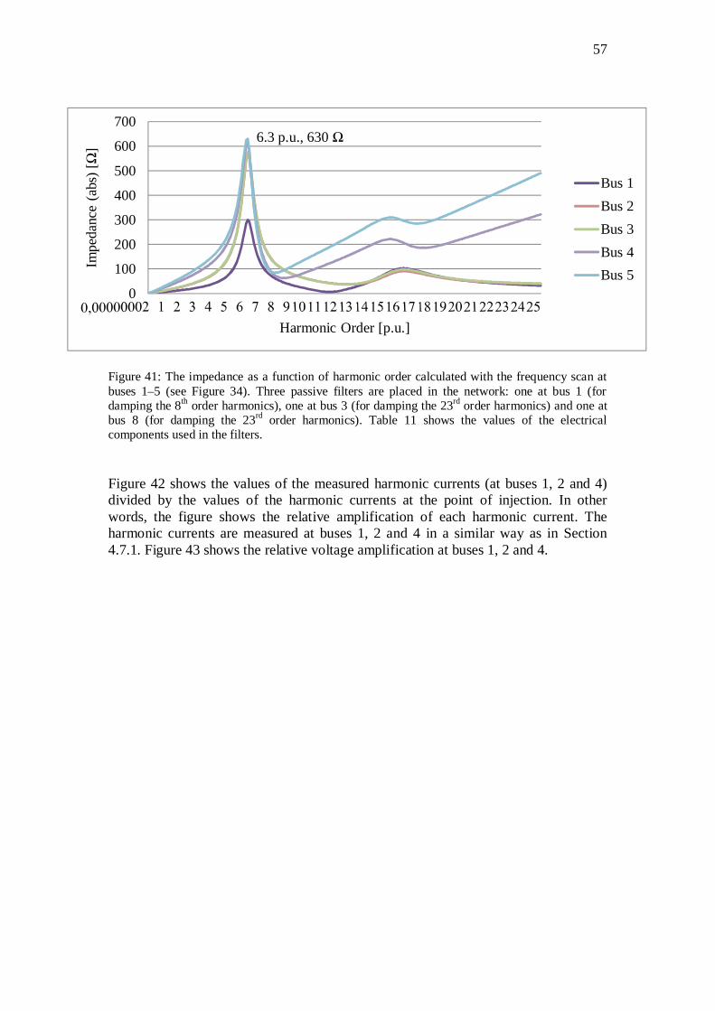
57
Figure 41: The impedance as a function of harmonic order calculated with the frequency scan at buses 1–5 (see Figure 34). Three passive filters are placed in the network: one at bus 1 (for damping the 8th order harmonics), one at bus 3 (for damping the 23rd order harmonics) and one at bus 8 (for damping the 23rd order harmonics). Table 11 shows the values of the electrical components used in the filters. Figure 42 shows the values of the measured harmonic currents (at buses 1, 2 and 4) divided by the values of the harmonic currents at the point of injection. In other words, the figure shows the relative amplification of each harmonic current. The harmonic currents are measured at buses 1, 2 and 4 in a similar way as in Section 4.7.1. Figure 43 shows the relative voltage amplification at buses 1, 2 and 4.
6.3 p.u., 630
0
100
200
300
400
500
600
700
Impe
danc
e (a
bs) [
]
Harmonic Order [p.u.]
Bus 1Bus 2Bus 3Bus 4Bus 5

58
Figure 42: Measured harmonic currents compared to the injected harmonic currents. The currents are measured the buses 1, 2 and 4 (see Figure 34).
Figure 43: Measured harmonic voltages at buses 1, 2 and 4 divided by the corresponding harmonic voltages at bus 5. See the order of the buses in Figure 34. The voltage waveforms before and after placing the filters can be seen in Figures 44 and 45. The voltages are measured at bus 2. The first waveform is without any filters (as in Section 4.7.1) and the second is with the passive filters (as in this section). The curves are obtained from the PSCAD software simulations.
0
0,2
0,4
0,6
0,8
1
1,2
1,4
1,6
2 4 5 7 8 10 11 12 13 14 16 17 18 19 20 22 23 24 25
Volta
ge /
Volta
ge a
t Bus
5 [p
.u.]
Harmonic Order [p.u.]
Bus 4Bus 2Bus 1
0
5
10
15
20
25
2 4 5 7 8 10 11 12 13 14 16 17 18 19 20 22 23 24 25
Cur
rent
/ In
ject
ed C
urre
nt [p
.u.]
Harmonic Order [p.u.]
Bus 4Bus 2Bus 1

59
Figure 44: The voltage waveform at bus 2 (see Figure 34) in the case with no filters (as in the simulations of Section 4.7.1).
Figure 45: The voltage waveform at bus 2 (see Figure 34) after placing the passive filters to the network (as in the simulations of this section).
4.8 The Impact of Skin Effect on Modal Analysis
Skin effect is always present at high frequency currents. An interesting question is if it has a significant effect on the modal analysis. In many harmonic analyses, skin effect is taken into account especially when modelling cables. The objective of this section is to study if it is important to take the skin effect into account in the harmonic resonance mode analysis. The skin effect is considered in the cables, the components where it usually has the greatest significance. The higher the frequency, the stronger is the skin effect. This means that with higher frequencies the current tends to flow more on the surface of the conductor and the resistance becomes higher. In different cable structures the skin effect appears slightly differently, and here it is taken into account with an equation that varies according to cable type. [94] In this simulation, the resistance R of the cable at a certain harmonic order is calculated as

60
= (0.187 + 0.532 ), (22)
where is the resistance of the cable at the fundamental frequency and ( 2.35) is the harmonic order [1]. Because the skin effect affects only resistances and not inductances or capacitances (that are the main components in resonances), a general conclusion could be drawn that including the skin effect in calculations does not shift the resonance frequencies. However, the increasing resistance could damp the impedance peaks at resonance points. The modal analysis is calculated with the aggregated wind power as shown in Figures 8 and 9. Curves of the four most critical modal impedances are shown in Figure 46. Table 13 presents the bus participation factors.
Figure 46: The four most critical modes when the skin effect of the cables is taken into account. The value of X refers to the harmonic order (the horizontal axis) and the value of Y refers to the absolute value of the modal impedance (the vertical axis). The modal impedance curve of the second critical mode cannot be seen, since it is behind the third critical mode as in Figure 10 (see the bus participation factors of the second and the third critical modes in Table 13). The harmonic analysis is calculated with the network shown in Figures 8 and 9. The bus participation factors are presented in Table 13. The order of the buses can be seen in Figure 34.

61
The
Criti
calit
y of
Mod
e1
23
45
67
89
1011
1213
1415
1617
1819
20
The
Num
ber
of
Mod
e7
1920
814
179
1516
1018
1112
136
53
42
1H
arm
onic
O
rder
[p.u
.]8.
4120
12.12
8012
.128
08.
4130
12.1
170
12.1
2712
.322
12.1
212
.113
12.3
3612
.316
13.4
13.5
1413
.577
10.4
9710
.953
13.7
3213
.964
18.5
5425
Freq
uenc
y [H
z]42
0.6
606.
460
6.4
420.
6560
5.85
606.
3561
6.160
660
5.65
616.
861
5.8
670
675.
767
8.85
524.
8554
7.65
686.
669
8.2
927.
712
50Th
e M
axim
um
Abs
olut
e V
alue
of
Mod
al
Impe
danc
e [
]
1.525
E+07
1.059
E+07
1.05
9E+0
79.
883E
+06
8.05
4E+0
67.
890E
+06
6.29
7E+0
63.
491E
+06
2.515
E+06
6.825
E+05
5.88
4E+0
49.
173E
+03
8.36
8E+0
37.
985E
+03
1.92
8E+0
31.3
53E+
032.1
89E+
021.
968E
+02
6.06
4E+0
12.
596E
+00
Bus
Pa
rtic
ipat
ion
Fact
ors Bu
s 1
0.02
900.0
000
0.000
00.
0290
0.00
000.
0000
0.00
530.
0000
0.00
000.0
053
0.000
00.
0027
0.00
250.
0024
0.11
180.
1581
0.69
030.
7222
0.94
830.
0002
Bus
20.
0445
0.000
00.0
000
0.04
450.
0000
0.00
000.
0007
0.00
000.
0000
0.000
70.0
000
0.00
000.
0000
0.00
000.
0798
0.09
030.
0829
0.077
30.0
194
0.66
42Bu
s 3
0.04
470.0
000
0.000
00.
0448
0.00
000.
0000
0.00
060.
0000
0.00
000.0
006
0.000
00.
0000
0.00
000.
0000
0.07
880.
0884
0.07
580.0
702
0.015
20.
1678
Bus
40.
0471
0.001
40.0
001
0.04
710.
0008
0.00
100.
0000
0.00
080.
0008
0.000
00.0
009
0.00
050.
0006
0.00
060.
0566
0.05
530.
0123
0.010
20.0
004
0.00
00Bu
s 5
0.04
780.0
030
0.000
20.
0478
0.00
160.
0022
0.00
020.
0016
0.00
160.0
002
0.002
00.
0011
0.00
120.
0013
0.05
010.
0464
0.00
520.0
040
0.000
00.
0000
Bus
60.
0490
0.010
50.0
005
0.04
900.
0054
0.00
780.
0026
0.00
540.
0054
0.002
60.0
070
0.00
440.
0046
0.00
460.
0401
0.03
380.
0012
0.000
80.0
000
0.00
00Bu
s 7
0.06
530.
4875
0.024
80.
0653
0.24
220.
3609
0.24
540.
2422
0.24
220.
2454
0.33
010.
2433
0.24
300.
2429
0.01
580.
0082
0.00
000.0
000
0.000
00.
0000
Bus
80.
0471
0.001
40.0
001
0.04
710.
0008
0.00
100.
0000
0.00
080.
0008
0.000
00.0
009
0.00
050.
0006
0.00
060.
0566
0.05
530.
0123
0.010
20.0
004
0.00
00Bu
s 9
0.04
780.0
030
0.000
20.
0478
0.00
160.
0022
0.00
020.
0016
0.00
160.0
002
0.002
00.
0011
0.00
120.
0013
0.05
010.
0464
0.00
520.0
040
0.000
00.
0000
Bus
100.
0490
0.010
50.0
005
0.04
900.
0054
0.00
780.
0026
0.00
540.
0054
0.002
60.0
070
0.00
440.
0046
0.00
460.
0401
0.03
380.
0012
0.000
80.0
000
0.00
00Bu
s 11
0.06
530.
4875
0.024
80.
0653
0.24
220.
3609
0.24
540.
2422
0.24
220.
2454
0.33
010.
2433
0.24
300.
2429
0.01
580.
0082
0.00
000.0
000
0.000
00.
0000
Bus
120.
0447
0.000
00.0
000
0.04
480.
0000
0.00
000.
0006
0.00
000.
0000
0.000
60.0
000
0.00
000.
0000
0.00
000.
0788
0.08
840.
0758
0.070
20.0
152
0.16
78Bu
s 13
0.04
710.0
001
0.001
40.
0471
0.00
080.
0007
0.00
000.
0008
0.00
080.0
000
0.000
60.
0005
0.00
060.
0006
0.05
660.
0553
0.01
230.0
102
0.000
40.
0000
Bus
140.
0478
0.000
20.0
030
0.04
780.
0016
0.00
150.
0002
0.00
160.
0016
0.000
20.0
013
0.00
110.
0012
0.00
130.
0501
0.04
640.
0052
0.004
00.0
000
0.00
00Bu
s 15
0.04
900.0
005
0.010
50.
0490
0.00
540.
0052
0.00
260.
0054
0.00
540.0
026
0.004
50.
0044
0.00
460.
0046
0.04
010.
0338
0.00
120.0
008
0.000
00.
0000
Bus
160.
0653
0.024
80.
4875
0.06
530.
2422
0.24
140.
2454
0.24
220.
2422
0.24
540.2
113
0.24
330.
2430
0.24
290.
0158
0.00
820.
0000
0.000
00.0
000
0.00
00Bu
s 17
0.04
710.0
001
0.001
40.
0471
0.00
080.
0007
0.00
000.
0008
0.00
080.0
000
0.000
60.
0005
0.00
060.
0006
0.05
660.
0553
0.01
230.0
102
0.000
40.
0000
Bus
180.
0478
0.000
20.0
030
0.04
780.
0016
0.00
150.
0002
0.00
160.
0016
0.000
20.0
013
0.00
110.
0012
0.00
130.
0501
0.04
640.
0052
0.004
00.0
000
0.00
00Bu
s 19
0.04
900.0
005
0.010
50.
0490
0.00
540.
0052
0.00
260.
0054
0.00
540.0
026
0.004
50.
0044
0.00
460.
0046
0.04
010.
0338
0.00
120.0
008
0.000
00.
0000
Bus
200.
0653
0.024
80.
4875
0.06
530.
2422
0.24
140.
2454
0.24
220.
2422
0.24
540.2
113
0.24
330.
2430
0.24
290.
0158
0.00
820.
0000
0.000
00.0
000
0.00
00
Tabl
e 13
: All
of th
e bu
s par
ticip
atio
n fa
ctor
s in
the
case
, whe
re th
e sk
in e
ffec
t is t
aken
into
ac
coun
t in
the
cabl
es. S
ee th
e or
der o
f the
bus
es 9
. The
hig
hest
val
ues
of th
e pa
rtici
patio
n fa
ctor
s of
eac
h m
ode
are
bold
ed.

62
5 Analysis of the Results
In this chapter all the results obtained from the simulations (Chapter 4) are analysed. In the first section (Section 5.1), the results from the basic configuration of the aggregated wind power plant are investigated. Section 5.2 examines the cases where the lengths of the collector and the transmission cables are changed. After this, in Section 5.3, the effect of the passive and the active filters on the resonance points is studied. Section 5.4 analyses the results of the harmonic current and voltage measurements. Lastly, in Section 5.5, it is commented how the skin effect affects the modal analysis.
5.1 Resonance Analysis of the Wind Power Plant
The bus participation factors in Table 4 clearly show that the aggregated wind power plant has the majority of its resonance points between the 12th and 13th harmonic (between 600 Hz and 650 Hz) although the critical resonance lies at the harmonic order of 23.75 per unit. The critical mode also has another peak at the frequency of 8.412 per unit (see Figure 10). Figure 10 shows that in this case considering only the four most critical modes (of the twenty modes) provides a clear idea of the resonance frequencies of the network. Table 4 presents the participation factors, where the critical mode is present in several buses, but the bus pairs 4 and 5, 8 and 9, 13 and 14, 17 and 18 (see Figure 9) are the ones that have the strongest participation in the resonance. In other words, these buses are the centres of the critical mode. Therefore the resonance of the critical mode occurs between the capacitances of the collector cables and the inductances of the generator transformers and the three winding transformers (see Figure 8). All these three components form together the conditions for a parallel resonance. To damp this resonance, the optimal locations to insert filtering are the buses with the highest participation factors, which in this case would be buses 4, 8, 13 and 17. Because the resonance exists in other buses as well, placing filters at these buses only would not damp the resonance totally. Observing the participation factors of the 2nd, 3rd, 4th and 5th most critical modes in Table 4, it is easy to notice that buses 7, 11, 16 and 20 are the ones most participating in these resonance modes. All four of these modes are very close to each other in terms of the maximum value of the modal impedance as well as in regard to their resonance frequency (that is near the 12th harmonic). These resonances could be damped rather effectively just by placing filters (tuned to 600 Hz) at buses 7, 11, 16 and 20. The same buses participate in the major part of the resonance modes, all of which are situated around the 12th and 13th order. It is important to point out that in this case the output filters (LCL filters) are problematic since they cause significant resonances. It is interesting to notice that the 2nd and 3rd critical modes (in Table 4) are identical what it comes to the resonance frequency and the maximum value of the modal impedance. The bus participation factors are identical, but the images are the reverse of each other. The participation factors of the 3rd critical mode at buses 13–20 are the same as the participation factors of the 2nd critical mode at buses 4–11 (see Figure 9). Likewise, the participation factors of the 3rd critical mode at buses 4–11 are the same

63
as the participation factors of the 2nd critical mode at buses 13–20. This is due to the symmetry of the network. Typically, the least important modes are not real resonances since they are inductances whose impedance increases naturally along with the growing frequency, as we can see in the case of the last mode (Table 4). As the network is very symmetric, a lot of symmetry can be noticed in the participation factors. The frequency scan is performed at all buses 1–7 (see Figure 11). The graphs given by the frequency scan support the results of the modal analysis indicating that the most important resonances lie at 8.4 per unit, 12.1 per unit and 23.7 per unit. It is important to highlight that the impedance peaks from the frequency scan are much lower in comparison with the modal impedances as they are different matters and are not directly comparable with each other. More information about their mutual connection is available in Chapter 3.
5.2 The Effect of Collector and Transmission Cable Lengths on
Resonance Points
The resonance points are near each other in cases when the length of the collector cable is 8 or 16 kilometres (see Figure 10 and 15). The highest point of the critical modal impedance is shifted about 100 Hz down and the other peak of the same mode experiences only a minimal shift in the same direction. The absolute values of the modal impedances decrease slightly. The area with many modal resonance peaks (around the 12th harmonic) experiences just minimal changes, what is observable from the participation factors is that the resonances around the 12th harmonic are concentrated in a slightly narrower frequency range when the collector cables have the length of 16 kilometres (see Tables 4 and 5). The graphs of the frequency scans also show that the peak at 23.7 per unit moves to 22 per unit (see Figures 11, 13 and 14). It is interesting that the impedance peak at bus 7 (at 12 per unit) increases remarkably (see Figures 11 and 14), although, the figure of the modal curves shows that they decrease. Even if the modal impedance peaks of the individual modes decrease, they are concentrated closer on each other (in terms of frequency) and their effect in a particular bus (in this case the bus 7) is superposed. The bus participation factors (in Tables 4 and 5) prove this statement. When the collector cables length increases to 32 kilometres, small changes in the location and the absolute value of the modal impedances can be noticed. As a general rule, all the resonance peaks move towards lower frequencies when the length of 33 kV cables increases. That is due to the greater shunt capacitances of the cables. Mathematically this phenomenon can be explained by Equation (9). The highest modal impedance can be found at 7.873 per unit. The maximum values of all the modal impedances decrease slightly. The frequency scan shows that the high impedance peak at bus 7 also decreases. When the collector cables in branches 1 and 3 (see Figures 8 and 9) have more length than the collector cables in branches 2 and 4, there are no any significant changes in the resonance frequencies (see Figures 17 and 19, and Tables 1 and 2 in Appendix A). The trend is similar to the earlier cases: as the cables gain more length (the cables have higher shunt capacitance) the resonance frequencies shift slightly

64
lower resonance frequencies. The most significant change is at about 2 per unit (100 Hz). When the length of the 150 kV transmission cables increases the resonance frequencies move towards lower frequencies but the shifts are moderate (see Figures 10 and 21). The greatest difference can be seen in the impedance of the frequency scan in the peaks at around 12 per unit. As the transmission cables length increase, the most of the impedance peaks lower significantly (see Figures 21 and 22, and Tables 1 and 2 in Appendix B). In the bus participation factors this effect is noticed as the modal impedance peaks around that area move fractionally away from each other and the effect of summation is not that strong as in the case of Section 4.3.
5.3 Adding Filters at Critical Buses
A second-order passive filter is located at buses 7, 11, 16 and 20 (one filter at each bus). See the order of the buses in Figure 9. Before adding the filters, the buses had strong resonances around the 12th harmonic. According to Figures 26 and 27 the passive filtering causes the disappearance of all the problematic resonance frequencies. The remaining resonances are split up into two groups: the group of higher frequencies is situated between the 22nd and the 24th order and the group of lower frequencies between the 2nd and the 3rd harmonic order. The group of higher frequencies also has a peak at the frequency of 9.1 per unit. The four most important resonances are situated in the higher frequency frame (see Table 7). These resonances are relatively dispersed, although, buses 5, 9, 14 and 18 can be identified as the centres of these resonances. The results of the frequency scan support this conclusion (Figure 27) showing that buses 5 and 6 participate strongly in the resonances at the 23.5th harmonic. Several new resonances appear in the lower frequency interval between the 2nd and the 3rd harmonic order. The participation factors show that buses 7, 11, 16 and 20 continue their complicated behaviour as they are the ones most involving in these new low frequency resonances. The results of the frequency scan in Figure 27 reveal that bus 7 has an important part in the resonance at 2.3 per unit as the other buses hardly participate in these resonances. It seems that rather than merely damping the resonance between the capacitance and the inductances of the LCL filter, the passive filters add more capacitance in parallel with the existing capacitance at buses 7, 11, 16 and 20 (see Figure 9). Because of the added capacitance, several resonance frequencies shift to the lower frequencies (see Table 7). This is the same effect that was seen before when increasing the length of the collector cables in Section 4.3. It is true that these resonance frequencies are partially damped as their peaks of the modal impedance are lower than before adding the filters (see Table 7). After placing the passive filters by the hybrid ones, the resonance peaks have similar frequencies, but their modal impedances are lower. This fact can be observed in Figures 32 and 33. What is important to consider is that the hybrid filters show better performance than the passive filters. Because the resonance modes are spread up in wide area, it is not impossible, even with the best filters, to damp them perfectly by placing only one filter at each branch of collector cables (see Figures 8 and 9). In

65
comparison with the case of passive filter resonances (Table 7) there are no significant changes in the group of the higher frequency, besides the descent of the maximum modal impedances. The impedance peaks in the group of lower frequency resonances descent as well but also shift about 1 per unit lower between the fundamental frequency and 2nd harmonic order.
5.4 Harmonic Current and Voltage Analyses
The modifications in the grid with the removal of the LCL filters (see the network in Figure 34) changed some characteristics of the network, although not drastically. When comparing the curves of the modal analyses of the cases with the LCL filters (Figure 10) and without (Figure 35) them, what is noticeable is that the critical modes have two peaks that do not change their place drastically after excluding the LCL filters from the grid model. In addition, the bus participation factors show that the second most important resonance area is around 12 per unit in the case with the LCL filters (Table 4) and around 10.4 per unit in the case without the LCL filters (Table 10). From the bus participation factors of the case without the LCL filters (Table 10) what must be taken considered is that the critical mode has outstandingly high modal impedance compared with the other modes. Moreover, the mode is spread over all the buses of the network, meaning that several filters will be needed to damp this mode efficiently. The second critical mode is divided among all the buses as well, but the maximum modal impedance of this mode is distinctly smaller than the impedance of the critical mode. The rest of the modes are not real resonance modes as they are just naturally growing impedances that increment along the growing frequency. The impedance graph given by the frequency scan (Figure 36) corresponds perfectly to the one from the modal analysis (Figure 35); they both have two peaks of the same orders. Figure 37 compares the measured harmonic currents (measured at buses 1, 2 and 4) to the injected harmonic currents. What is noticeable is that the form of the current amplification follows perfectly the form of the curve of the critical mode (Figure 35). The same form repeats in the impedance calculated by the frequency scan (Figure 36). Bus 1 amplifies the harmonic currents at around the 8th and 22nd harmonic while the bus 2 amplifies the currents around the 22nd and 23rd harmonic. The 8th harmonic current is multiplied by almost 40 times at bus 1 and the 22nd harmonic current by almost 50 times at bus 2. Compared with buses 1 and 2, bus 4 has just a small effect of amplification on the 22nd order. All this means that the most important areas to damp are the 8th and 22nd harmonic in the buses 1 and 2, respectively. The bus participation factors in Table 10 indicate placing the filter at bus 5 in order to damp the critical mode. Just by paying attention to the maximum values of the participation factors the peak of the critical mode at around the 8.5th harmonic cannot be noticed. Since one mode can have several impedance peaks, all the peaks of each mode have to be taken into account and not only the highest ones. Otherwise it may happen that some resonances leave without attention. Figure 38 and 39 present the voltage amplification and show that the most of the voltages is not amplified or are amplified little. The only exception is the 11th harmonic voltage that is amplified significantly in all of the buses 1, 2 and 4. The 11th harmonic corresponds to the second most critical mode. The amplification of this

66
mode can be observed clearly in Figure 39, which shows the relative increment of each harmonic voltage. This graph is totally different from the one of the current amplification (Figure 37). The voltage increases significantly at buses 1, 2 and 4. Mostly at bus 1, less at bus 2 and even less at bus 4. This result corresponds well to the bus participation factors (the column of the second most critical mode in Table 10), which are 0.1303 for bus 1, 0.0981 for bus 2 and 0.0746 for bus 4. If we compare these participation factors with the one of the bus 5, that is 0.0698, we can say that the harmonic voltages increase when going from a bus with the smaller bus participation factor to a bus with the greater participation factor (for the same mode) (see Table 10). The voltages around the 8th and 23nd harmonic do not increase because the values of the bus participation factors decrease when going from bus 5 to bus 4, bus 2 or bus 1 (the column of the critical mode in Table 10). The role of the bus participation factors in the voltage analysis certainly requires further research. After adding the three passive filters (one of for a damping the resonance at 400 Hz and two for damping the resonances at 1150 Hz, see Table 11), in Section 4.7.2, the highest peak of the critical mode can be found at 6.495 per unit and the same mode has also one lower peak at 16 per unit (Figures 40 and 41). A comparison of the filter results with the non-filter results reveals that the modal impedance of the critical mode has decreased remarkably. The filters do their task and damp the resonances at the 8th and 22nd harmonics, but also introduce new resonances at 6.495 per unit and 16 per unit, even though these peaks are significantly lower than the highest non-filter peaks (Figures 35 and 36). The same conclusion can be drawn from the graph of the frequency scan presented in Figure 41, although the highest peaks of the frequency scan are slightly shifted in comparison with the curve of the modal analysis. The form of the figure of the current amplification (Figure 42) corresponds very well to the curve of the modal impedance of the critical mode. The current that increased the most is the 7th harmonic. In addition, the 5th and 8th harmonic currents are significantly high. The currents after the 17th harmonic do not show any high increments. Before placing the filters, the highest current amplification was almost 50 times the injected current, after placing the filtering the highest current amplification is about 20 times the injected current (Figure 42). Moreover, bus 1 is responsible for this high value of the current. After placing the passive filters, the harmonic voltages (Figure 43) are better damped than before the filtering. This can be noticed in the bus participation factors in Table 12. At the 11th harmonic, the high peaks do not exist anymore. In fact, the peak around the 8th harmonic that is the only area where the voltages increase compared to their value at bus 5. The value of the voltage before the 7th harmonic is the highest at bus 4, the next at bus 2 and the smallest at bus 1. This case corresponds to the critical mode that has its bus participation factors in the same order of magnitude. In a similar manner, the voltages between the 10th and 12th harmonic correspond to the 6th critical mode. Again, after the 14th harmonic the critical mode becomes more dominating and the voltages are amplified more at buses 2 and 4 than at bus 1. In a similar way, the voltage amplification at the 16th harmonic corresponds to the 10th most critical mode. The harmonics that are between the resonance peaks and that do not seem corresponding clearly to any of the modes are probably mixes of different modes. More tangible improvement in voltage waveforms at bus 2 can be seen in Figures 44 and 45.

67
5.5 Impact of the Skin Effect on Modal Analysis
The skin effect is considered in the cable resistances. The curves of the modal impedances (Figure 46) show that the highest peaks are at the same locations as in Figure 10. Because the skin effect has a greater impact on higher frequencies, what can be noticed is that after including the skin effect the critical peak can be found at 8.412 per unit. The maximum values of all the modal impedances have descended. In this case only minimalistic changes can be noticed after taking into account the skin effect. For example the 6th and 4th as well as the 5th and 7th modes have changed their places in the table of the participation factors (Table 13). The changes are small and do not virtually have any impact on the resonance modes.
6 Discussion
According to the case studies presented in this thesis, the shunt capacitance of an underground cable system is the dominating element in the resonances of a wind power plant. A change in the length of the collector cables moves the resonance frequencies. As a general rule, the greater the capacitance of an (capacitive) element is, the lower are the resonance frequencies. What must be considered is that the cables do not resonate alone since they need an interaction with an inductive element to create a resonance. Typically this element is a (electrically) near locating transformer due to its large inductance. Passive filters are technically simple and fairly efficient damping the harmonics. However, they still have one remarkable inconvenience: not only do they usually damp the problematic frequency but they also introduce new resonance frequency to the network. That is why all potential secondary effects have to be investigated thoroughly when planning any passive filtering. The symmetry of a network can be noticed in the participation factors. The more symmetry there is in the network, the more the modal impedance peaks with similar resonance frequencies. It also appears that the modal impedance peaks are more concentrated into groups. Moreover, in symmetric grids one mode can have several centres of frequency. Likewise, there may be several modes that are exactly equal in terms of both resonance frequency and maximum absolute value of the modal impedance. In these cases, the bus participation factors of the modes are reversed or in a different order. Furthermore, the frequency scan does not see the individual modes since it calculates the sum of the modal impedances at certain point of the network. If there are several modes with similar resonance frequency, the impedance calculated by the frequency scan has the higher peak at that point. In other words, an effect of summation is observable in the result of the frequency scan. The harmonic mode analysis offers more information about the resonances than the traditional frequency scan. In addition, it is applicable to distribution as well as transmission systems. It also provides a wide insight into the power system resonances. Hence, the harmonic resonance modal analysis could be taken to form a part of systematic grid resonance and harmonic analysis. Although the modal analysis proves extremely useful, it has one inconvenience. The amount of information obtained increases significantly with the size of the network.

68
This increase is caused by the size of the admittance matrix and the number of participation factors growing proportionally to the square of the number of the buses. In the investigated case, the skin effect does not have any great effect on the modal analysis. According to the findings in the present study, it is not important to consider the skin effect in the harmonic studies below the 26th harmonic. Probably the skin effect has more importance at higher frequencies. It is still unclear how large a modal impedance peak must be to be considered significant. This certainly is dependent on the network configuration. However, more knowledge in this area is needed in order to implement the harmonic modal analysis as part of a systematic harmonic and resonance analysis. Because the simulation results have not been validated with any real life measurements, it is unknown whether they are near the real values. What is known is that the model of the aggregated wind power plant is quite rough, so the results cannot be exactly the same as in the real life. Thus, hopefully, they are sufficient to provide directional results. If there are any significant errors, they are probably related to the inaccuracy of the component models. One possible source of error is that each cable is presented as one -element, and presenting cables as several -elements in series could increase the accuracy of the simulations. Transformers also play an important role in the resonances and they could be modelled in a more detailed manner in order to obtain more exact results.
7 Conclusions and Future Work
This chapter states the final conclusions of the thesis and presents ideas how the work done in this thesis can be continued forward.
7.1 Conclusions
Electrical resonance in a power network can be a complex phenomenon where several components participate. Filtering is the most usual way for damping resonances and it can be said, that hybrid filters offer better performance than passive filters. Hybrid filters are technically more complex since they are equipped with a control and a controlled voltage source. The harmonic resonance mode analysis is a relatively new method in the network resonance analysis and it shows great usefulness when solving resonance problems. The harmonic mode analysis is a promising tool and reveals the grid resonance points effectively. It greatest inconvenience is that in the case of a large power system, the large amount of data makes the analysis of a power system laborious. Furthermore, efficient and reliable calculation algorithms are needed to identify the resonances.
7.2 Future Work
The reliability and the accuracy of the harmonic resonance mode analysis need to be verified with real life measurements in power systems. The harmonic resonance mode analysis detects the parallel resonances in a power system (that is the major resonance problem), but it could be completed to detect the

69
series resonances as well. The role and the physical meaning of the participation factors needs further investigation. A systematic and reliable automatic calculation algorithm based on the harmonic modal analysis would facilitate the resonance analysis of the distribution and transmission networks and help to identify the optimal locations for filters.

70
References
[1] J. Arrillaga and W. Neville," Power System Harmonics", ISBN: 0470851295, West Sussex: Wiley & Sons, 2003. [2] D. L. Rosa, "Harmonics and Power Systems", ISBN: 0849330165, Boca Raton, FL: CRC/Taylor & Francis, 2006. [3] L. Sainz, "Deterministic and Stochastic Study of Wind Farm Harmonic Currents," Energy Conversion, IEEE Transactions on, pp. 1071, 2010. [4] J. Elovaara and L. Haarla, "Sähköverkot 1: Järjestelmätekniikka ja sähköverkon laskenta", ISBN: 9789516723603, Helsinki: Otatieto, 2011. [5] N. Mohan, "Power Electronics Converters, Applications and Design", ISBN: 0471226939, Wiley, 2002. [6] R. E. Brown, "Electric Power Distribution Reliability", ISBN: 0849375673, Boca Raton, FL: CRC Press, 2009. [7] J. Elovaara and Y. Laiho, "Sähkölaitostekniikan Perusteet", ISBN: 9789516722859, Helsinki: Otatieto, 1999. [8] A. B. Baggini, "Handbook of Power Quality", ISBN: 0470065613, Chichester, England: John Wiley & Sons, 2008. [9] K. Dettmann, S. Schostan and D. Schulz, "Wind Turbine Harmonics Caused by Unbalanced Grid Currents", Electrical Power Quality and Utilisation, 13(2), 2007. [10] G. Atkinson-Hope, "Relationship Between Harmonics and Symmetrical Components", International Journal of Electrical Engineering Educators (IJEEE), vol. 2, April, 2004. [11] G. J. Wakileh, "Power System Harmonics - Fundamentals, Analysis and Filter Design", ISBN: 3540422382, Springer, 2001. [12] C. Sankaran, "Power Quality", ISBN: 0849310407, Boca Raton, FL: CRC Press, 2002. [13] H. K. Lukasz, J. Hjerrild and C. L. Bak, "Harmonic Models of a Back-to-Back Converter in Large Offshore Wind Farms Compared with Measurement Data", Nordic Wind Power Conference 2009, Bornholm, Denmark, 2009. [14] E. W. Gunther, "Interharmonics in Power Systems", IEEE Power Engineering Society Summer Meeting 2001, 2001, pp. 813–817 vol. 2.

71
[15] D. Patel, "Impact of Wind Turbine Generators on Network Resonance and Harmonic Distortion," Electrical and Computer Engineering (CCECE), 2010 23rd Canadian Conference on, 2010. [16] I. Arana, L. Kocewiak, J. Holboll, L. Bak and A. H. Nielsen, "How to Improve the Design of the Electrical System in Future Wind Power Plant", Nordic Wind Power Conference (NWPC2009), Bornholm, Denmark, 2009. [17] H. D. Young and R.A. Freedman, "Sears and Zemansky's University Physics with Modern Physics", ,ISBN: 0201603365, San Francisco: Addison-Wesley, 2011. [18] R. Zheng, "Harmonic Resonances Due to a Grid-Connected Wind Farm", Harmonics and Quality of Power (ICHQP), 14th International Conference on, Bergamo, Italy, pp. 1, 2010. [19] M. Aro, J. Elovaara, M. Karttunen, K. Nousiainen, V. Palva, "Suurjännitetekniikka", ISBN: 9789516723207, Helsinki: Otatieto, 2003. [20] H. K. Lukasz, J. Hjerrild and C. L. Bak, "Harmonic Analysis of Offshore Wind Farms with Full Converter Wind Turbines", 8th International Conference on Large-Scale Integration of Wind Power into Power Systems, Bremen, Germany, 2009. [21] B. Fox, D. Flynn, M. O´Malley, L. Bryans and R. Watson, "Wind Power Integration Connection and System Operational Aspects", Stevenage: Institution on Engineering and Technology, 2007. [22] S. T. Tentzerakis, "An Investigation of the Harmonic Emissions of Wind Turbines", Energy Conversion, IEEE Transactions on, 2007, pp. 150. [23] H. Sik Kim and D. D. Lu, "Wind Energy Conversion System from Electrical Perspective - A Survey", SGRE, 2010, pp. 127-131. [24] A. Kusko, "Power Quality in Electrical Systems", ISBN: 0071470751, McGraw-Hill Professional Publishing: Blacklick, OH, USA, 2007. [25] L. Xiaodong and W. M. Jackson, "Influence of Subsea Cables on Offshore Power Distribution Systems", Industry Applications, IEEE Transactions on, 2009, vol. 45, pp. 2136-2144. [26] S. R. Samantaray and P. K. Dash, "Transmission Line Distance Relaying Using Machine Intelligence Technique", Generation, Transmission & Distribution, The Institution of Engineering and Technology (IET), vol. 2, 2008, pp. 53–61. [27] S. Tentzerakis, S. Papathanassiou, P. Papadopoulos, D. Foussekis and P. Vionis, "Evaluation of Wind Farm Harmonic Current Emissions", European Wind Energy Conference (EWEC), Milan, Italy, 2007. [28] T. Ackermann, "Wind Power in Power Systems", ISBN: 0470855088, Chichester, West Sussex, England: John Wiley, 2005.

72
[29] Jun Li, N. Samaan and S. Williams, "Modeling of Large Wind Farm Systems for Dynamic and Harmonics Analysis", Transmission and Distribution Conference and Exposition, T&D, IEEE/PES, 2008, pp. 1–7. [30] M. Chaves, E. Margato, J. F. Silva, S. F. Pinto and J. Santana, "Fast Optimum-Predictive Control and Capacitor Voltage Balancing Strategy for Bipolar Back-to-Back NPC Converters in High-Voltage Direct Current Transmission Systems", Generation, Transmission & Distribution, The Institution of Engineering and Technology (IET), vol. 5, pp. 368–375, 2011. [31] S. Liang, Q. Hu and W. Lee, "A Survey of Harmonic Emissions of a Commercial Operated Wind Farm", Industrial and Commercial Power Systems Technical Conference (I&CPS), IEEE, 2010, pp. 1–8.
[32] B. Babypriya, A. Chilambuchelvan. "Modelling and Analysis of DFIG Wind Turbine Harmonics Generated in Grids", International Journal of Engineering and Technology (IJET), ISSN: 0975-4024, 2(3), June 2010, pp. 185–189.
[33] J. Hu, H. Nian, H. Xu and Y. He, "Dynamic Modeling and Improved Control of DFIG Under Distorted Grid Voltage Conditions", Energy Conversion, IEEE Transactions on, March 2011, vol. 26, pp. 163–175. [34] D. D. Banham-Hall, G. A. Taylor, C. A. Smith and M. R. Irving, "Towards Large-Scale Direct Drive Wind Turbines with Permanent Magnet Generators and Full Converters", Power and Energy Society General Meeting, 2010 IEEE, ISSN: 1944-9925, Minneapolis, USA, 25-29 July 2010, pp. 1–8. [35] A. T. Alexandridis and G. E. Marmidis, "Modeling Wind Generators with Full-Scale Frequency Converters: Stability and Passivity Properties", Power Generation, Transmission, Distribution and Energy Conversion (MedPower 2010), 7th Mediterranean Conference and Exhibition on, Agia Napa, Cyprus, 2010, pp. 1–5. [36] L. Kocewiak, L. Bak and J. Hjerrild, "Harmonic Aspects of Offshore Wind Farms", PhD Seminar on Detailed Modelling and Validation of Electrical Components and Systems 2010, Fredericia, Denmark, 2010, p. 40–45. [37] M. H. J. Bollen, S. Cundeva, S. K. Rönnberg, M. Wahlberg, Kai Yang and Liangzhong Yao, "A Wind Park Emitting Characteristic and Non-Characteristic Harmonics", Power Electronics and Motion Control Conference (EPE/PEMC) 14th International, 2010, pp. S14–22–S14–26. [38] L. Kocewiak, J. Hjerrild and L. Bak., "The Impact of Harmonics Calculation Methods on Power Quality Assessment in Wind Farms", ISBN: 978-1-4244-7244-4, Bergamo, Italy, 2010, pp. 1–9. [39] S. Tentzerakis, N. Paraskevopoulou, S. Papathanassiou and P. Papadopoulos, "Measurement of Wind Farm Harmonic Emissions", IEEE Power Electronics Specialists Conference (PESC 2008), Rhodes, Greece, 15-19 June 2008, pp. 1769-1775.

73
[40] Z. Jie and B. Guangqing, "Voltage Stability Improvement for Large Wind Farms Connection Based on VSC-HVDC", Power and Energy Engineering Conference (APPEEC) 2011, Wuhan, China, 2011, pp. 1-4. [41] E. Sheeba Percis, L. Ramesh, R. Rakesh, V. Gobinath and S. P. Chowdhury, "The Impact of BoBC in Off-Shore Wind Energy Conversion System," Computer, Communication and Electrical Technology (ICCCET) 2011, International Conference on, Tamil Nadu, India, 18-19 March 2011, pp. 424-429. [42] D. M. Mohan, B. Singh and B. K. Panigrahi, "A New Control Strategy for Active and Reactive Power Control of Three-Level VSC Based HVDC system," India Conference (INDICON) 2010, Annual IEEE, 2010, pp. 1-4. [43] Chung-ming Young, Ming-hui Chen, Chien-hsiang Lai and Der-Chun Shih, "A Novel Control for Active Interphase Transformer Using in a 24-Pulse Converter", Power Electronics Conference (IPEC), 2010 International, 2010, pp. 2086-2091. [44] D. Madhan Mohan, B. Singh and B. K. Panigrahi, "Harmonic Optimised 24-Pulse Voltage Source Converter for High Voltage DC Systems", Power Electronics IET, vol. 2, ISSN: 1755-4535, September 2009, pp. 563–573. [45] J. Jafarzadeh, M. T. Haq, S. M. Mahaei and P. Farhadi, "Optimal Placement of FACTS Devices Based on Network Security", Computer Research and Development (ICCRD), 2011 3rd International Conference on, ISBN: 978-1-61284-839-6, Shanghai, China, 2011, pp. 345–349. [46] S. N. Keshmiri, A. Jamehbozorg and G. Radman, "Optimum Reactive Power Compensation Regime for Radial Connected Wind Turbines", Southeastcon 2011 Proceedings of IEEE, ISSN: 1091-0050, Nashville, USA, 17-20 March 2011, pp. 24–29. [47] M. P. Donsión, J. A. Güemes and F. Oliveira, "Influence of a SVC on AC Arc Furnaces Harmonics, Flicker and Unbalance Measurement and Analysis", 15th IEEE Mediterranean Electrotechnical Conference (MELECON 2010), 2010, pp. 1423-1428. [48] P. Chopade, M. Bikdash, I. Kateeb and A. D. Kelkar, "Reactive Power Management and Voltage Control of Large Transmission System Using SVC (Static VAR Compensator)," Southeastcon, 2011 Proceedings of IEEE, ISSN: 1091-0050, Nashville, USA, 17-20 March 2011, pp. 85–90. [49] N. G. Hingorani, "Understanding FACTS Concepts and Technology of Flexible AC Transmission Systems", ISBN: 0780334558, Piscataway, USA: IEEE Press, 2000. [50] K. E. Okedu, S. M. Muyeen, R. Takahashi and J. Tamura, "Participation of FACTS in Stabilizing DFIG with Crowbar During Grid Fault Based on Grid Codes," GCC Conference and Exhibition (GCC), 2011 IEEE, 2011, pp. 365–368.

74
[51] K. E. Okedu, S. M. Muyeen, R. Takahashi and J. Tamura, "Comparative Study of Wind Farm Stabilization Using Variable Speed Generator and FACTS Device," GCC Conference and Exhibition (GCC), 2011 IEEE, 2011, pp. 569–572. [52] Z. Bingjie, W. Xiaojie, F. Xiao and D. Peng, "A Novel 12-pulse 3-level Inverter for STATCOM Using Selective Harmonic Elimination Modulation," Power and Energy Engineering Conference (APPEEC), ISBN: 978-1-4244-4812-8, Chengdu, China, 28–31 March 2010, pp. 1–5. [53] H. K. Lukasz, J. Hjerrild and C. L. Bak, "Wind Farm Structures´ Impact on Harmonic Emission and Grid Interaction", European Wind Energy Conference 2010, Warsaw, Poland, 2010. [54] C. H. Chien, "Theoretical Aspects of the Harmonic Performance of Subsea AC Transmission Systems for Offshore Power Generation Schemes," Generation, Transmission and Distribution, IEE Proceedings- , 2006. [55] B. Normark and E. Nielsen, "Advanced Power Electronics for Cable Connection of Offshore Wind", ABB, Copenhagen, Denmark, 2005. [56] S. Heier, "Grid Integration of Wind Energy Conversion Systems", ISBN: 047197143X, Chichester: Wiley, 2006. [57] F. Shewarega, I. Erlich and J. L. Rueda, "Impact of Large Offshore Wind Farms on Power System Transient Stability," Power Systems Conference and Exposition (PSCE '09), IEEE/PES, 2009, pp. 1–8. [58] M. Bradt, B. Badrzadeh, E. Camm, D. Mueller, T. Siebert, T. Smith and M. Starke, "Harmonics and Resonance Issues in Wind Power Plants,", IEEE Power and Energy Society - Wind Plant Collector System Design Working Group, 2010. [59] L. Qiang, H. Zhiyuan and T. Guangfu, "Investigation of the Harmonic Optimization Approaches in the New Modular Multilevel Converters," Power and Energy Engineering Conference (APPEEC), ISBN: 978-1-4244-4812-8, Chengdu, China, 28–31 March 2010, pp. 1–6. [60] S. A. Papathanassiou and M. P. Papadopoulos, "Harmonic Analysis in a Power System with Wind Generation", Power Delivery, IEEE Transactions on, 2006, vol. 21, pp. 2006-2016. [61] E. Muljadi, C. P. Butterfield, J. Chacon and H. Romanowitz, "Power Quality Aspects in a Wind Power Plant," IEEE Power Engineering Society General Meeting, ISBN: 1-4244-0493-2, Montreal, Canada, 2006. [62] R. Dugan, M. McGranagh, S. Santoso and W. Beaty, "Electrical Power Systems Quality", ISBN: 007138622X, New York: McGraw-Hill, 2003. [63] R. S. Vedam and M. Sarma, "Power Quality - VAR Compensation in Power Systems", ISBN: 1420064800, Boca Raton, FL: Chapman & Hall/CRC, 2009.

75
[64] M. H. Abdel-Rahman, "Power Quality and Harmonics - Post-Graduate Course", Aalto University School of Electrical Engineering, Espoo, Finland, 17 November 2010. [65] S. Qiang, J. Junpeng, T. Huan and C. Guitao, "Design of Active Power Filter for Low Voltage and High Current Switching Power Supply," Power and Energy Engineering Conference (APPEEC), ISSN: 2157-4839, Wuhan, China 25–28 March, 2011, pp. 1–4. [66] D. Li and J. Tian, "A Novel Active Power Filter for the Voltage Source Type Harmonic Source," Electrical Machines and Systems, International Conference on (ICEMS 2008), Wuhan, China, 17–20 October 2008, pp. 2077–2080. [67] C. Junling, L. Yaohua, W. Ping, Y. Zhizhu and D. Zuyi, "A Novel Combined System Using Cascaded Active Power Filter and Static var Compensator for High-Power Applications," Computer Distributed Control and Intelligent Environmental Monitoring (CDCIEM), 2011 International Conference on, ISBN: 978-1-61284-278-3, Changsha, China, 19–20 February 2011, pp. 664–667. [68] W. Zhao, Z. Shangli and A. Luo, "A New Injection Type Hybrid Active Power Filter and Its Application," Measuring Technology and Mechatronics Automation (ICMTMA), 2011 Third International Conference on, ISBN: 978-1-4244-9010-3, Shangshai, China, 6–7 January 2011, pp. 162–165. [69] Z. Tang and D. Liao, "The Research and Simulation of Shunt Hybrid Active Power Filter Based on PSCAD/EMTDC," Energy and Environment Technology, (ICEET '09), International Conference on, ISBN: 978-0-7695-3819-8, Guilin, China, 2009, pp. 352–356. [70] F. Z. Peng and D. J. Adams, "Harmonic Sources and Filtering Approaches-Series/Parallel, Active/Passive, and Their Combined Power Filters," IEEE Industry Applications Conference, Thirty-Fourth IAS Annual Meeting, Conference Record of the 1999, pp. 448–455, vol.1. [71] H. Fujita, T. Yamasaki and H. Akagi, "A Hybrid Active Filter for Damping of Harmonic Resonance in Industrial Power Systems," Power Electronics Specialists Conference (PESC 98) 29th Annual IEEE, 1998, pp. 209–216, vol.1. [72] P. Maibach, A. Faulstich, M. Eichler and S. Dewar, "Full-Scale Medium-Voltage Converters for Wind Power Generators up to 7 MVA," ABB Switzerland Ltd, www.abb.com, 2009. [73] S. V. Araujo, A. Engler, B. Sahan and F. Antunes, "LCL-filter Design for Grid-Connected NPC Inverters in Offshore Wind Turbines," Power Electronics (ICPE '07), 7th Internatonal Conference on, ISBN: 978-1-4244-1871-8, Daegu, South Korea, 22–26 October 2007, pp. 1133–1138. [74] A. A. Rockhill, M. Liserre, R. Teodorescu and P. Rodriguez, "Grid-Filter Design for a Multimegawatt Medium-Voltage Voltage-Source Inverter," Industrial Electronics, IEEE Transactions on, 2011, vol. 58, pp. 1205–1217.

76
[75] Z. Huang, Y. Cui and W. Xu, "Application of Modal Sensitivity for Power System Harmonic Resonance Analysis," Power Systems, IEEE Transactions on, vol. 22, 2007, pp. 222–231. [76] C. Chang, S. Chan and J. Teng, "A Fast Method for Driving Point Impedance Calculation of Unbalanced Distribution System", IEEE International Conference on Systems & Signals (ICSS 2005), 2005, pp. 134–138. [77] J. C. Das, "Power System Analysis Short-Circuit Load Flow and Harmonics", ISBN: 0824707370, New York: Marcel Dekker, 2002. [78] J. Machowski, "Power System Dynamics Stability and Control", ISBN: 0470725583, Chichester, U.K.: Wiley, 2008. [79] Caixia Yang, Kaipei Liu and Dongxu Wang, "Harmonic resonance circuit's modeling and simulation," Power and Energy Engineering Conference, (APPEEC 2009), ISBN: 978-1-4244-2486-3, Wuhan, China, 27–31 March 2009, pp. 1–5. [80] D. C. Lay, "Linear Algebra and its Applications", ISBN: 0321314859, Boston: Pearson/Addison-Wesley, 2006. [81] C. Yang, K. Liu and Q. Zhang, "An Improved Modal Analysis Method for Harmonic Resonance Analysis," Industrial Technology, (ICIT 2008), IEEE International Conference on, ISBN: 978-1-4244-1705-6, Chengdu, China, 2008, pp. 1–5. [82] M. Esmaili, H. Ali Shayanfar and A. Jalilian, "Modal Analysis of Power Systems to Mitigate Harmonic Resonance Considering Load Models," Energy, vol. 33, 2008, pp. 1361–1368.
[83] K. Nisak, I. Candela, K. Rauma, J. R. Hermoso and A. Luna, "An Overview of Harmonic Analysis and Resonances of a Large Wind Power Plant", Annual Conference of the IEEE Industrial Electronics Society (IECON 2011), 7–10 November 2011.
[84] C. Amornvipas and L. Hofmann, "Resonance Analyses in Transmission Systems: Experience in Germany," IEEE Power and Energy Society General Meeting 2010, ISSN: 1944-9925, Minneapolis, USA, 25–29 July 2010, pp. 1–8. [85] X. Wilsun, H. Zhenyu, C. Yu and W. Haizhen, "Harmonic Resonance Mode Analysis", IEEE Power Engineering Society General Meeting, 2005, pp. 2236 Vol. 3. [86] G. Argüello and H. Flores, "Estudio de estabilidad de pequeña señal en el sistema nacional interconectado aplicando el método de análisis modal", XIX Jornadas de Ingeniería Eléctrica y Electrónica (JIEE), vol. 19, 2005, pp. 192–198. [87] H. Zhou, Y. Wu, S. Lou and X. Xiong, "Power system series harmonic resonance assessment based on improved modal analysis", UI - JEEE 7(2), 2007, pp. 423-430.

77
[88] Yu Cui and Wilsun Xu, "Harmonic Resonance Mode Analysis Using Real Symmetrical Nodal Matrices," Power Delivery, IEEE Transactions on, 2007, vol. 22, pp. 1989-1990. [89] S. K. Chaudhary, R. Teodorescu, P. Rodriguez and P. C. Kjaer, "Control and Pperation of Wind Turbine Converters During Faults in an Offshore Wind Power Plant Grid with VSC-HVDC Connection", IEEE Power and Energy Society General Meeting, 2011, pp. 1–8. [90] W. Xu, "Status and future directions of power system harmonic analysis", IEEE Power Engineering Society General Meeting 2004, ISBN: 0-7803-7989-6, March 2004, Vol.1, pp. 756–761. [91] J. I. Candela, "Aportaciones al filtrado híbrido paralelo en redes trifásicas de cuatro hilos", ISBN: 9788469443545, Technical University of Catalonia (UPC), Department of Electrical Engineering (DEE), 14 June 2009. [92] S. Srianthumrong and H. Akagi, "A Medium-Voltage Transformerless AC/DC Power Conversion System Consisting of a Diode Rectifier and a Shunt Hybrid Filter," Industry Applications, IEEE Transactions on, ISSN: 0093-9994, May–June 2003, vol. 39, pp. 874–882.
[93] A. A. Rockhill, M. Liserre, R. Teodorescu and P. Rodriguez, "Grid-Filter Design for a Multimegawatt Medium-Voltage Voltage-Source Inverter," Industrial Electronics, IEEE Transactions on, ISSN: 0278-0046, vol. 58, pp. 1205–1217, April 2011.
[94] C. H. Chien and R. Bucknall, "Harmonic Calculations of Proximity Effect on Impedance Characteristics in Subsea Power Transmission Cables," Power Delivery, IEEE Transactions on, ISSN: 0885-8977, vol. 24, October 2009, pp. 2150–2158.

78
Appendix A: The Bus Participation Factors of the Aggregated Wind Power Plant When the Lengths of the 33 kV Collector Cables are Changed
The C
ritic
ality
of
Mod
e1
23
45
67
89
1011
1213
1415
1617
1819
20
The N
umbe
r of
M
ode
1319
1718
2015
1614
128
97
1110
65
34
21
Harm
onic
O
rder
[p.u
.]8.
2790
12.11
8012
.290
012
.061
012
.0130
7.841
09.5
3325
11.32
911
.781
2513
.268
2525
12.0
1314
.68
14.6
825
2525
Freq
uenc
y [H
z]41
3.95
605.9
614.
560
3.05
600.
6539
2.05
476.
6512
5056
6.45
589.
0512
5066
3.4
1250
1250
600.
6573
473
412
5012
5012
50Th
e Max
imum
Ab
solu
te V
alue
of
Mod
al
Impe
danc
e []
6.82
4E+0
71.4
31E+
071.
321E
+07
1.21
3E+0
79.
593E
+06
1.44
8E+0
42.4
24E+
031.
372E
+03
9.72
9E+0
27.0
40E+
024.
354E
+02
2.741
E+02
2.38
4E+0
22.
332E
+02
1.877
E+02
1.47
4E+0
29.
551E
+01
5.84
7E+0
17.
574E
+00
2.596
E+00
Bus
Part
icip
atio
n Fa
ctor
s Bus 1
0.02
760.
0000
0.005
10.
0002
0.00
000.0
225
0.01
510.0
000
0.21
290.
2938
0.003
80.
6096
0.00
000.0
000
0.72
980.
7951
0.88
660.
0002
0.000
00.
0002
Bus 2
0.04
400.
0000
0.000
70.
0000
0.00
000.0
401
0.01
500.0
006
0.10
040.
1074
0.098
40.
0951
0.00
010.0
003
0.07
600.0
621
0.03
850.
0082
0.000
00.
6642
Bus 3
0.04
430.
0000
0.000
60.
0000
0.00
000.0
405
0.01
490.0
010
0.09
770.
1036
0.099
50.
0882
0.00
010.0
006
0.06
890.0
553
0.03
270.
0067
0.49
930.
1678
Bus 4
0.04
790.
0000
0.000
00.
0006
0.00
150.0
458
0.01
160.0
041
0.05
600.
0499
0.042
80.
0213
0.03
150.0
456
0.01
150.0
070
0.00
230.
0008
0.000
30.
0000
Bus 5
0.05
000.
0000
0.000
20.
0029
0.00
550.0
493
0.00
770.0
176
0.03
620.
0279
0.003
30.
0063
0.01
350.0
222
0.00
230.0
011
0.00
020.
0001
0.000
00.
0000
Bus 6
0.05
100.
0001
0.001
70.
0084
0.01
440.0
517
0.00
260.0
279
0.02
360.
0158
0.135
70.
0018
0.03
580.0
521
0.00
040.0
002
0.00
000.
0000
0.000
00.
0000
Bus 7
0.06
470.
0061
0.137
50.
3185
0.48
170.0
723
0.19
750.0
004
0.00
330.
0012
0.000
50.
0000
0.00
010.0
001
0.00
000.0
000
0.00
000.
0000
0.000
00.
0000
Bus 8
0.04
640.
0016
0.000
10.
0006
0.00
000.0
444
0.01
090.1
367
0.05
220.
0457
0.006
10.
0181
0.00
310.2
379
0.00
950.0
057
0.00
190.
3914
0.000
40.
0000
Bus 9
0.04
700.
0034
0.000
50.
0011
0.00
000.0
458
0.00
870.2
287
0.04
100.
0330
0.003
80.
0088
0.00
180.1
528
0.00
360.0
018
0.00
040.
3476
0.000
00.
0000
Bus 1
00.
0480
0.01
140.0
043
0.00
310.
0000
0.048
00.
0029
0.36
150.
0267
0.01
870.
1559
0.00
260.
0048
0.35
790.
0007
0.000
20.
0000
0.01
020.0
000
0.00
00Bu
s 11
0.06
090.
5124
0.36
130.
1193
0.00
130.0
672
0.22
310.0
056
0.00
380.
0014
0.000
60.
0000
0.00
000.0
005
0.00
000.0
000
0.00
000.
0000
0.000
00.
0000
Bus 1
20.
0443
0.00
000.0
006
0.00
000.
0000
0.040
50.
0149
0.000
30.
0978
0.10
370.0
995
0.08
830.
0002
0.000
10.
0689
0.055
30.
0327
0.00
810.
4993
0.16
78Bu
s 13
0.04
790.
0000
0.000
00.
0007
0.00
150.0
458
0.01
160.0
014
0.05
600.
0499
0.042
90.
0213
0.10
260.0
088
0.01
150.0
070
0.00
230.
0009
0.000
30.
0000
Bus 1
40.
0500
0.00
000.0
002
0.00
300.
0054
0.049
30.
0077
0.006
00.
0363
0.02
790.0
033
0.00
630.
0441
0.004
30.
0023
0.001
10.
0002
0.00
010.0
000
0.00
00Bu
s 15
0.05
100.
0000
0.001
70.
0088
0.01
420.0
517
0.00
260.0
095
0.02
360.
0158
0.135
70.
0018
0.11
650.0
100
0.00
040.0
002
0.00
000.
0000
0.000
00.
0000
Bus 1
60.
0648
0.00
000.1
376
0.33
350.
4728
0.07
240.
1976
0.000
10.
0033
0.00
120.0
005
0.00
000.
0002
0.000
00.
0000
0.000
00.
0000
0.00
000.0
000
0.00
00Bu
s 17
0.04
790.
0014
0.000
10.
0009
0.00
000.0
458
0.01
120.0
345
0.05
420.
0473
0.006
50.
0186
0.19
640.0
327
0.00
970.0
058
0.00
190.
1213
0.000
40.
0000
Bus 1
80.
0489
0.00
300.0
005
0.00
170.
0000
0.047
40.
0090
0.062
90.
0431
0.03
460.0
038
0.00
920.
1232
0.022
10.
0037
0.001
90.
0004
0.10
150.0
000
0.00
00Bu
s 19
0.04
990.
0101
0.004
10.
0050
0.00
000.0
498
0.00
310.0
994
0.02
810.
0196
0.156
80.
0027
0.32
550.0
518
0.00
070.0
003
0.00
000.
0030
0.000
00.
0000
Bus 2
00.
0634
0.45
040.3
431
0.19
150.
0016
0.069
70.
2321
0.001
50.
0039
0.00
150.0
006
0.00
000.
0005
0.000
10.
0000
0.000
00.
0000
0.00
000.0
000
0.00
00
Tabl
e 1:
The
bus
par
ticip
atio
n fa
ctor
s whe
n th
e 33
kV
cab
les o
f the
bra
nche
s 1 a
nd 3
hav
e th
e le
ngth
s of
16
kilo
met
res a
nd th
e br
anch
es 2
and
4 h
ave
8 ki
lom
etre
s lon
gitu
de. T
he h
ighe
st v
alue
s of
the
parti
cipa
tion
fact
ors
of e
ach
mod
e ar
e bo
lded
for m
akin
g re
adin
g ea
sier
. Thi
s tab
le c
orre
spon
ds to
Fi
gure
17
in S
ectio
n 4.
3.
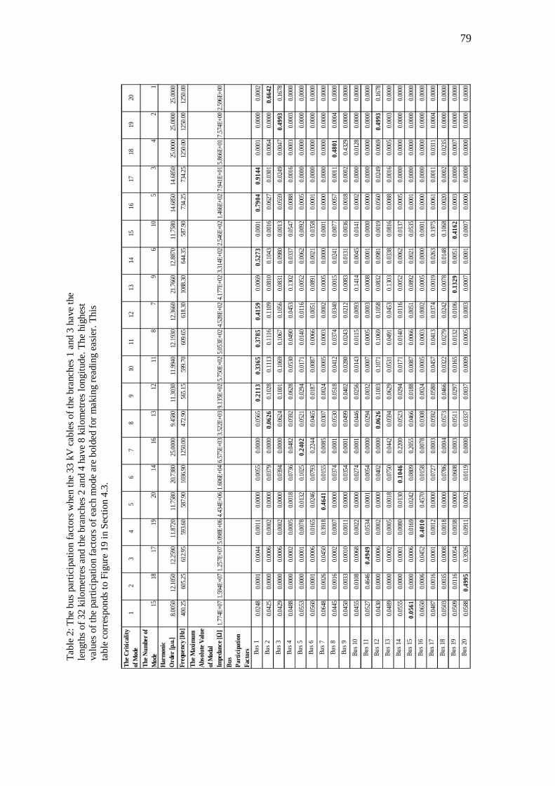
79
The C
ritic
ality
of
Mod
e1
23
45
67
89
1011
1213
1415
1617
1819
20
The N
umbe
r of
Mod
e15
1817
1920
1416
1312
118
79
610
53
42
1Ha
rmon
ic
Ord
er [p
.u.]
8.005
012
.1050
12.25
9011
.8720
11.75
8020
.7380
25.00
009.4
580
11.30
3011
.9940
12.19
3012
.3660
21.76
6012
.8870
11.75
8014
.6850
14.68
5025
.0000
25.00
0025
.0000
Freq
uenc
y [Hz
]40
0.25
605.2
561
2.95
593.6
058
7.90
1036
.9012
50.00
472.9
056
5.15
599.7
060
9.65
618.3
010
88.30
644.3
558
7.90
734.2
573
4.25
1250
.0012
50.00
1250
.00Th
e Max
imum
Ab
solu
te Va
lue
of M
odal
Im
peda
nce [
]1.7
74E+
071.5
94E+
071.2
57E+
075.0
98E+
064.4
34E+
061.6
06E+
046.5
75E+
033.5
22E+
039.1
35E+
025.7
50E+
025.0
53E+
024.5
28E+
024.1
77E+
023.3
14E+
022.5
46E+
021.4
66E+
027.9
41E+
015.8
66E+
017.5
74E+
002.5
96E+
00Bu
s Pa
rtici
patio
n Fa
ctor
s Bus 1
0.024
80.0
001
0.004
40.0
011
0.000
00.0
055
0.000
00.0
565
0.21
130.
3365
0.37
850.
4159
0.006
90.
5273
0.000
10.
7904
0.91
440.0
001
0.000
00.0
002
Bus 2
0.042
50.0
000
0.000
60.0
002
0.000
00.0
379
0.000
00.
0626
0.102
80.1
113
0.111
60.1
109
0.081
00.1
043
0.001
60.0
627
0.030
10.0
064
0.000
00.
6642
Bus 3
0.042
90.0
000
0.000
60.0
002
0.000
00.0
394
0.000
00.0
624
0.100
10.1
069
0.106
70.1
056
0.083
10.0
980
0.001
30.0
559
0.024
90.0
047
0.49
930.1
678
Bus 4
0.048
80.0
000
0.000
20.0
005
0.001
80.0
736
0.048
20.0
592
0.062
80.0
530
0.049
00.0
453
0.130
20.0
337
0.054
70.0
088
0.001
60.0
003
0.000
30.0
000
Bus 5
0.055
30.0
000
0.000
10.0
078
0.013
20.1
025
0.24
020.0
521
0.029
40.0
171
0.014
00.0
116
0.005
20.0
062
0.009
20.0
005
0.000
00.0
000
0.000
00.0
000
Bus 6
0.056
00.0
001
0.000
60.0
165
0.024
60.0
793
0.224
40.0
465
0.018
70.0
087
0.006
60.0
051
0.089
10.0
021
0.035
80.0
001
0.000
00.0
000
0.000
00.0
000
Bus 7
0.064
80.0
026
0.045
00.3
918
0.46
410.0
155
0.008
50.0
307
0.002
40.0
005
0.000
30.0
002
0.000
50.0
000
0.000
10.0
000
0.000
00.0
000
0.000
00.0
000
Bus 8
0.044
50.0
016
0.000
20.0
007
0.000
00.0
374
0.000
10.0
530
0.051
80.0
412
0.037
40.0
340
0.001
50.0
241
0.007
70.0
057
0.001
10.
4801
0.000
40.0
000
Bus 9
0.045
00.0
033
0.001
00.0
011
0.000
00.0
354
0.000
10.0
499
0.040
20.0
280
0.024
30.0
212
0.008
30.0
131
0.003
60.0
018
0.000
20.4
329
0.000
00.0
000
Bus 1
00.0
455
0.010
80.0
068
0.002
20.0
000
0.027
40.0
001
0.044
60.0
256
0.014
30.0
115
0.009
30.1
414
0.004
50.0
141
0.000
20.0
000
0.012
80.0
000
0.000
0Bu
s 11
0.052
70.4
646
0.49
490.0
534
0.000
10.0
054
0.000
00.0
294
0.003
20.0
007
0.000
50.0
003
0.000
80.0
001
0.000
00.0
000
0.000
00.0
000
0.000
00.0
000
Bus 1
20.0
430
0.000
00.0
006
0.000
20.0
000
0.040
20.0
000
0.06
260.1
003
0.107
10.1
069
0.105
80.0
832
0.098
10.0
019
0.056
00.0
249
0.006
90.
4993
0.167
8Bu
s 13
0.048
90.0
000
0.000
20.0
005
0.001
80.0
750
0.044
20.0
594
0.062
90.0
531
0.049
10.0
453
0.130
30.0
338
0.081
60.0
088
0.001
60.0
005
0.000
30.0
000
Bus 1
40.0
555
0.000
00.0
001
0.008
00.0
130
0.10
460.2
200
0.052
30.0
294
0.017
10.0
140
0.011
60.0
052
0.006
20.0
137
0.000
50.0
000
0.000
00.0
000
0.000
0Bu
s 15
0.05
610.0
000
0.000
60.0
169
0.024
20.0
809
0.205
50.0
466
0.018
80.0
087
0.006
60.0
051
0.089
20.0
021
0.053
50.0
001
0.000
00.0
000
0.000
00.0
000
Bus 1
60.0
650
0.000
60.0
452
0.40
100.4
570
0.015
80.0
078
0.030
80.0
024
0.000
50.0
003
0.000
20.0
005
0.000
00.0
001
0.000
00.0
000
0.000
00.0
000
0.000
0Bu
s 17
0.048
70.0
016
0.000
10.0
012
0.000
00.0
727
0.000
30.0
592
0.058
00.0
457
0.041
30.0
374
0.001
90.0
263
0.197
50.0
061
0.001
10.0
311
0.000
40.0
000
Bus 1
80.0
503
0.003
50.0
008
0.001
80.0
000
0.078
60.0
004
0.057
30.0
466
0.032
20.0
279
0.024
20.0
078
0.014
80.1
068
0.002
00.0
002
0.023
50.0
000
0.000
0Bu
s 19
0.050
90.0
116
0.005
40.0
038
0.000
00.0
608
0.000
30.0
511
0.029
70.0
165
0.013
20.0
106
0.13
290.0
051
0.41
620.0
003
0.000
00.0
007
0.000
00.0
000
Bus 2
00.0
588
0.49
950.3
926
0.091
10.0
002
0.011
90.0
000
0.033
70.0
037
0.000
90.0
005
0.000
30.0
007
0.000
10.0
007
0.000
00.0
000
0.000
00.0
000
0.000
0
Tabl
e 2:
The
bus
par
ticip
atio
n fa
ctor
s whe
n th
e 33
kV
cab
les o
f the
bra
nche
s 1 a
nd 3
hav
e th
e le
ngth
s of
32
kilo
met
res a
nd th
e br
anch
es 2
and
4 h
ave
8 ki
lom
etre
s lon
gitu
de. T
he h
ighe
st
valu
es o
f the
par
ticip
atio
n fa
ctor
s of e
ach
mod
e ar
e bo
lded
for m
akin
g re
adin
g ea
sier
. Thi
s ta
ble
corr
espo
nds t
o Fi
gure
19
in S
ectio
n 4.
3.

80
Appendix B: The Bus Participation Factors of the Aggregated Wind Power Plant When the Lengths of the 150 kV Transmission Cables are Changed
The C
ritic
ality
of
Mod
e1
23
45
67
89
1011
1213
1415
1617
1819
20
The N
umbe
r of
Mod
e8
1920
914
715
1716
1012
1118
136
54
32
1Ha
rmon
ic
Ord
er [p
.u.]
7.69
8012
.128
012
.1280
12.29
4012
.1060
19.24
8012
.1080
12.13
1012
.065
012
.2040
12.77
1012
.8490
13.95
8025
.0000
12.10
6010
.518
010
.5180
13.87
2015
.2950
25.00
00Fr
eque
ncy [
Hz]
384.
9000
606.4
000
606.4
000
614.7
000
605.3
000
962.4
000
605.4
000
606.
5500
603.2
500
610.2
000
638.5
500
642.4
500
697.9
000
1250
.0000
605.3
000
525.9
000
525.9
000
693.6
000
764.7
500
1250
.0000
The M
axim
um
Abso
lute
Val
ue
of M
odal
Im
peda
nce [
]3.0
33E+
072.1
44E+
072.
144E
+07
1.365
E+07
1.304
E+07
6.340
E+06
5.442
E+06
3.531
E+06
2.671
E+05
1.03
0E+0
52.0
24E+
041.7
49E+
046.4
08E+
031.3
89E+
031.3
41E+
031.1
99E+
032.
276E
+02
1.880
E+02
1.160
E+02
5.237
E+00
Bus
Part
icip
atio
n Fa
ctor
s Bus 1
0.02
610.0
000
0.000
00.0
041
0.000
00.0
156
0.000
00.
0000
0.000
00.0
043
0.003
40.0
033
0.000
00.0
000
0.11
800.
1327
0.61
700.
6823
0.82
080.0
006
Bus 2
0.04
840.0
000
0.000
00.0
006
0.000
00.0
622
0.000
00.
0000
0.000
00.0
007
0.000
20.0
002
0.000
00.0
000
0.09
420.0
983
0.105
50.0
945
0.062
70.6
567
Bus 3
0.04
920.0
000
0.000
00.0
005
0.000
00.0
672
0.000
00.
0000
0.000
00.0
005
0.000
10.0
001
0.000
00.0
005
0.09
150.0
950
0.090
60.0
793
0.048
80.
1712
Bus 4
0.05
060.0
013
0.000
10.0
000
0.000
80.
0673
0.000
80.
0014
0.000
80.0
000
0.000
20.0
002
0.001
10.0
471
0.05
800.0
573
0.015
60.0
110
0.003
70.0
001
Bus 5
0.05
100.0
028
0.000
20.0
003
0.001
70.0
648
0.001
70.
0030
0.001
70.0
003
0.000
70.0
008
0.002
50.0
782
0.04
890.0
473
0.006
90.0
043
0.000
90.0
000
Bus 6
0.05
120.0
097
0.000
80.0
029
0.005
60.0
515
0.005
60.
0104
0.005
60.0
027
0.003
70.0
038
0.009
10.
1225
0.03
590.0
336
0.001
70.0
008
0.000
10.0
000
Bus 7
0.05
390.
4504
0.038
80.
2453
0.24
190.0
134
0.24
190.
4818
0.24
180.
2455
0.24
440.
2442
0.49
670.0
019
0.00
830.0
066
0.000
00.0
000
0.000
00.0
000
Bus 8
0.05
060.0
013
0.000
10.0
000
0.000
80.
0673
0.000
80.
0014
0.000
80.0
000
0.000
20.0
002
0.001
10.0
471
0.05
800.0
573
0.015
60.0
110
0.003
70.0
001
Bus 9
0.05
100.0
028
0.000
20.0
003
0.001
70.0
648
0.001
70.
0030
0.001
70.0
003
0.000
70.0
008
0.002
50.0
782
0.04
890.0
473
0.006
90.0
043
0.000
90.0
000
Bus 1
00.
0512
0.009
70.0
008
0.002
90.0
056
0.051
50.0
056
0.01
040.0
056
0.002
70.0
037
0.003
80.0
091
0.12
250.
0359
0.033
60.0
017
0.000
80.0
001
0.000
0Bu
s 11
0.05
390.
4504
0.038
80.
2453
0.24
190.0
134
0.24
190.
4818
0.24
180.
2455
0.24
440.
2442
0.49
670.0
019
0.00
830.0
066
0.000
00.0
000
0.000
00.0
000
Bus 1
20.
0492
0.000
00.0
000
0.000
50.0
000
0.067
20.0
000
0.00
000.0
000
0.000
50.0
001
0.000
10.0
000
0.000
50.
0915
0.095
00.0
906
0.079
30.0
488
0.17
12Bu
s 13
0.05
060.0
001
0.001
30.0
000
0.000
80.
0673
0.000
80.
0000
0.000
80.0
000
0.000
20.0
002
0.000
00.0
471
0.05
800.0
573
0.015
60.0
110
0.003
70.0
001
Bus 1
40.
0510
0.000
20.0
028
0.000
30.0
017
0.064
80.0
017
0.00
000.0
017
0.000
30.0
007
0.000
80.0
000
0.078
20.
0489
0.047
30.0
069
0.004
30.0
009
0.000
0Bu
s 15
0.05
120.0
008
0.009
70.0
029
0.005
60.0
515
0.005
60.
0001
0.005
60.0
027
0.003
70.0
038
0.000
20.
1225
0.03
590.0
336
0.001
70.0
008
0.000
10.0
000
Bus 1
60.
0539
0.038
80.
4504
0.24
530.
2419
0.013
40.
2419
0.00
560.
2418
0.24
550.
2444
0.24
420.0
096
0.001
90.
0083
0.006
60.0
000
0.000
00.0
000
0.000
0Bu
s 17
0.05
060.0
001
0.001
30.0
000
0.000
80.
0673
0.000
80.
0000
0.000
80.0
000
0.000
20.0
002
0.000
00.0
471
0.05
800.0
573
0.015
60.0
110
0.003
70.0
001
Bus 1
80.
0510
0.000
20.0
028
0.000
30.0
017
0.064
80.0
017
0.00
000.0
017
0.000
30.0
007
0.000
80.0
000
0.078
20.
0489
0.047
30.0
069
0.004
30.0
009
0.000
0Bu
s 19
0.05
120.0
008
0.009
70.0
029
0.005
60.0
515
0.005
60.
0001
0.005
60.0
027
0.003
70.0
038
0.000
20.
1225
0.03
590.0
336
0.001
70.0
008
0.000
10.0
000
Bus 2
00.
0539
0.038
80.
4504
0.24
530.
2419
0.013
40.
2419
0.00
560.
2418
0.24
550.
2444
0.24
420.0
096
0.001
90.
0083
0.006
60.0
000
0.000
00.0
000
0.000
0
Tabl
e 1:
The
bus
par
ticip
atio
n fa
ctor
s whe
n th
e 15
0 kV
tran
smis
sion
cab
les a
re 1
16 k
ilom
etre
s lon
g.
The
high
est v
alue
s of
the
parti
cipa
tion
fact
ors o
f eac
h m
ode
are
bold
ed fo
r mak
ing
read
ing
easi
er.
This
tabl
e co
rres
pond
s to
Figu
re 2
1 in
Sec
tion
4.4.

81
The C
ritic
ality
of
Mod
e1
23
45
67
89
1011
1213
1415
1617
1819
20
The N
umbe
r of
Mod
e19
209
1417
87
1516
1011
1812
135
64
32
1Ha
rmon
ic
Ord
er [p
.u.]
12.12
8012
.1280
12.27
0012
.0950
12.12
907.0
780
7.080
012
.1000
12.03
4012
.3620
12.44
7011
.2900
11.12
4010
.3140
12.12
9010
.2480
10.24
8013
.2320
13.74
5025
.0000
Freq
uenc
y [Hz
]60
6.460
6.461
3.560
4.75
606.4
535
3.935
460
560
1.761
8.162
2.35
564.5
556.2
515.7
606.4
551
2.451
2.466
1.668
7.25
1250
The M
axim
um
Abso
lute
Val
ue
of M
odal
Im
peda
nce [
]2.1
44E+
072.1
44E+
071.0
82E+
071.0
36E+
079.2
80E+
068.4
46E+
063.0
47E+
062.0
31E+
061.8
13E+
051.0
41E+
055.4
52E+
041.2
65E+
041.0
90E+
045.7
17E+
031.0
06E+
039.6
49E+
022.4
98E+
022.1
99E+
021.8
00E+
028.0
64E+
00Bu
s Pa
rtic
ipat
ion
Fact
ors Bu
s 10.0
000
0.000
00.0
033
0.000
00.0
000
0.023
80.0
238
0.000
00.0
000
0.003
30.0
032
0.000
00.0
000
0.000
00.
1205
0.12
620.
5096
0.55
870.
6338
0.001
2Bu
s 20.0
000
0.000
00.0
005
0.000
00.0
000
0.050
80.0
509
0.000
00.0
000
0.000
40.0
003
0.000
00.0
000
0.000
00.1
079
0.109
70.1
329
0.127
00.1
148
0.64
40Bu
s 30.0
000
0.000
00.0
003
0.000
00.0
000
0.052
20.0
522
0.000
00.0
000
0.000
30.0
002
0.000
00.0
000
0.000
00.1
028
0.104
30.1
104
0.103
50.0
904
0.177
1Bu
s 40.0
013
0.000
10.0
001
0.000
90.0
013
0.053
00.0
530
0.000
90.0
009
0.000
10.0
001
0.001
50.0
010
0.001
10.0
581
0.057
70.0
213
0.017
40.0
122
0.000
1Bu
s 50.0
027
0.000
30.0
005
0.001
80.0
027
0.05
310.
0531
0.001
80.0
018
0.000
50.0
006
0.003
30.0
020
0.002
20.0
468
0.046
00.0
101
0.007
60.0
046
0.000
0Bu
s 60.0
095
0.001
10.0
032
0.005
80.0
097
0.052
60.0
526
0.005
80.0
058
0.003
30.0
035
0.011
20.0
063
0.006
70.0
318
0.030
80.0
028
0.001
80.0
009
0.000
0Bu
s 70.
4417
0.049
20.
2451
0.24
150.
4469
0.046
70.0
466
0.24
150.
2414
0.24
500.
2448
0.48
390.
2406
0.23
990.0
047
0.004
30.0
000
0.000
00.0
000
0.000
0Bu
s 80.0
013
0.000
10.0
001
0.000
90.0
013
0.053
00.0
530
0.000
90.0
009
0.000
10.0
001
0.001
50.0
010
0.001
10.0
581
0.057
70.0
213
0.017
40.0
122
0.000
1Bu
s 90.0
027
0.000
30.0
005
0.001
80.0
027
0.05
310.
0531
0.001
80.0
018
0.000
50.0
006
0.003
30.0
020
0.002
20.0
468
0.046
00.0
101
0.007
60.0
046
0.000
0Bu
s 10
0.009
50.0
011
0.003
20.0
058
0.009
70.0
526
0.052
60.0
058
0.005
80.0
033
0.003
50.0
112
0.006
30.0
067
0.031
80.0
308
0.002
80.0
018
0.000
90.0
000
Bus 1
10.
4417
0.049
20.
2451
0.24
150.
4469
0.046
70.0
466
0.24
150.
2414
0.24
500.
2448
0.48
390.
2406
0.23
990.0
047
0.004
30.0
000
0.000
00.0
000
0.000
0Bu
s 12
0.000
00.0
000
0.000
30.0
000
0.000
00.0
522
0.052
20.0
000
0.000
00.0
003
0.000
20.0
000
0.000
00.0
000
0.102
80.1
043
0.110
40.1
035
0.090
40.1
771
Bus 1
30.0
001
0.001
30.0
001
0.000
90.0
001
0.053
00.0
530
0.000
90.0
009
0.000
10.0
001
0.000
00.0
010
0.001
10.0
581
0.057
70.0
213
0.017
40.0
122
0.000
1Bu
s 14
0.000
30.0
027
0.000
50.0
018
0.000
30.
0531
0.05
310.0
018
0.001
80.0
005
0.000
60.0
000
0.002
00.0
022
0.046
80.0
460
0.010
10.0
076
0.004
60.0
000
Bus 1
50.0
011
0.009
50.0
032
0.005
80.0
011
0.052
60.0
526
0.005
80.0
058
0.003
30.0
035
0.000
00.0
063
0.006
70.0
318
0.030
80.0
028
0.001
80.0
009
0.000
0Bu
s 16
0.049
20.
4417
0.24
510.
2415
0.049
10.0
467
0.046
60.
2415
0.24
140.
2450
0.24
480.0
000
0.24
060.
2399
0.004
70.0
043
0.000
00.0
000
0.000
00.0
000
Bus 1
70.0
001
0.001
30.0
001
0.000
90.0
001
0.053
00.0
530
0.000
90.0
009
0.000
10.0
001
0.000
00.0
010
0.001
10.0
581
0.057
70.0
213
0.017
40.0
122
0.000
1Bu
s 18
0.000
30.0
027
0.000
50.0
018
0.000
30.
0531
0.05
310.0
018
0.001
80.0
005
0.000
60.0
000
0.002
00.0
022
0.046
80.0
460
0.010
10.0
076
0.004
60.0
000
Bus 1
90.0
011
0.009
50.0
032
0.005
80.0
011
0.052
60.0
526
0.005
80.0
058
0.003
30.0
035
0.000
00.0
063
0.006
70.0
318
0.030
80.0
028
0.001
80.0
009
0.000
0Bu
s 20
0.049
20.
4417
0.24
510.
2415
0.049
10.0
467
0.046
60.
2415
0.24
140.
2450
0.24
480.0
000
0.24
060.
2399
0.004
70.0
043
0.000
00.0
000
0.000
00.0
000
Tabl
e 2:
The
bus
par
ticip
atio
n fa
ctor
s whe
n th
e 15
0 kV
tran
smis
sion
cab
les a
re 1
74 k
ilom
etre
s lo
ng. T
he h
ighe
st v
alue
s of t
he p
artic
ipat
ion
fact
ors o
f eac
h m
ode
are
bold
ed fo
r mak
ing
read
ing
easi
er. T
his t
able
cor
resp
onds
to F
igur
e 23
in S
ectio
n 4.
4.