Electric Field Mapping (approx. 2 h 15 min.) (8/8/2018)

Equipment ● shallow glass pan● pitcher for water● masking tape● graph paper

(8.5”x14”)

● colored pencils● metal shapes● sand paper● paper towels● Graph paper

attached (print6 copies inadvance.

● DC power supplyPASCO 550 or 850interface

● Voltage probe with pointprobe & alligator clip

● rulers

● leads (2 banana-to- alligator; 1 banana- to-banana)

● “E-field probes”(optional use)

Introduction Positive and negative charges produce an “electric field”, E, at every point in space. The force experienced by a charge, q, in such an electric field is F = qE. Electric field lines begin and end on charges, since these are the sources of the electric field. We represent the electric field by vectors that point in the direction of the force that would occur on a positive “test” charge (left) and negative charge right. (see Fig. 1). The magnitude (strength) and direction (orientation) of the E field is observed with a positive “test charge” represented by the quantity qo. Wherever a test charge (qo) experiences an electric force, an electric field is present. The linked application below allows for you to experiment with charge configurations and the corresponding electric fields. Drag and drop positive and negative charges in space and “test” the field with the “sensor charge.” Leave the application running, we will return periodically throughout the experiment. Please complete this activity before entering the lab.

PhET Simulation: Charges and Fields https://phet.colorado.edu/en/simulation/charges-and-fields

Describe how the magnitude and direction of the Electric Field (E) varies based on: a) a single positive charge

b) a single negative charge

c) a dipole (a positive and a negative charge)

d) a line of positive charges (use multiple charges placed in a row)

e) a line of negative charges (use multiple charges placed in a row)

f) a line of positive and negative charges placed parallel to each other.

1

You probably noted E points away from positive charges and toward negative charges. As illustrated in Figure 1, electric field lines originate at positive charges and terminate at negative charges. In this lab, you will not measure the magnitude and direction of Electric Fields with positive “test charges” (qo), you will measure changes in the electric potential (voltage) in space. The magnitude of the the Electric Field is directly related to the lapse rate of the electric potential. You might ask, “What is the lapse rate of the the electric potential?” We will explain this using concepts you learned in your previous physics studies or everyday life.

Figure 1: Equipotentials and Electric Field Lines around a positive and negative point charge.

The analogy of a “hill” is useful in defining the concept of “lapse rates.” If a person were to ascend a gradual hill (slope) the change in vertical displacement per change in horizontal displacement is small. Alternatively, If a person were to ascend a steep hill (slope) the change in vertical displacement per change in horizontal displacement is large (compared to the gradual hill) .

Figure 3. Comparison of the slope for a small (15 feet) and large (45 feet) vertical displacement per similar horizontal displacement (100 feet). Our previous experience inform us that it requires a smaller effort (force) to ascend the first ramp compared to the second. Recalling content from Mechanics, the force parallel to the inclined place is F ∥ = mg sin Θ, therefore at greater angles relative to the horizontal, a greater applied force is required to move objects up or for you to walk up the inclined plane. Additionally, walking up both slopes requires work. The object moving up the steeper hill experiences a greater vertical displacement, therefore requires greater amounts of work to ascend the ramp, and lastly, experiences a greater change in potential energy. The gravitational potential energy change an object experiences is calculated using PE= mgΔh.

2

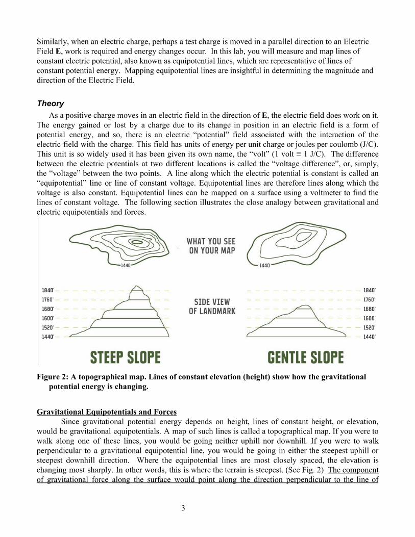
Similarly, when an electric charge, perhaps a test charge is moved in a parallel direction to an Electric Field E, work is required and energy changes occur. In this lab, you will measure and map lines of constant electric potential, also known as equipotential lines, which are representative of lines of constant potential energy. Mapping equipotential lines are insightful in determining the magnitude and direction of the Electric Field. Theory

As a positive charge moves in an electric field in the direction of E, the electric field does work on it. The energy gained or lost by a charge due to its change in position in an electric field is a form of potential energy, and so, there is an electric “potential” field associated with the interaction of the electric field with the charge. This field has units of energy per unit charge or joules per coulomb (J/C). This unit is so widely used it has been given its own name, the “volt” (1 volt ≡ 1 J/C). The difference between the electric potentials at two different locations is called the “voltage difference”, or, simply, the “voltage” between the two points. A line along which the electric potential is constant is called an “equipotential” line or line of constant voltage. Equipotential lines are therefore lines along which the voltage is also constant. Equipotential lines can be mapped on a surface using a voltmeter to find the lines of constant voltage. The following section illustrates the close analogy between gravitational and electric equipotentials and forces.

Figure 2: A topographical map. Lines of constant elevation (height) show how the gravitational potential energy is changing.

Gravitational Equipotentials and Forces

Since gravitational potential energy depends on height, lines of constant height, or elevation, would be gravitational equipotentials. A map of such lines is called a topographical map. If you were to walk along one of these lines, you would be going neither uphill nor downhill. If you were to walk perpendicular to a gravitational equipotential line, you would be going in either the steepest uphill or steepest downhill direction. Where the equipotential lines are most closely spaced, the elevation is changing most sharply. In other words, this is where the terrain is steepest. (See Fig. 2) The component of gravitational force along the surface would point along the direction perpendicular to the line of

3

constant elevation, in the steepest downhill direction. The more closely spaced the lines, the steeper the terrain, and the stronger the component of gravitational field along the surface.

Electric Equipotentials and Forces. Since there is no work associated with moving a charge along an electric equipotential, there is no net electric force in a direction along an electric equipotential line. Thus the component of the electric field vector E along an equipotential line must be zero. The direction of greatest rate of change in electric potential is the direction perpendicular to an electric potential line. Where the lines are most closely spaced, the electric potential energy is changing most sharply. In other words, this is where the electric force (and therefore the electric field) is strongest. The component of electric force (on a positive charge) along the surface points along the direction perpendicular to the line of constant electric potential, in the direction of sharpest decrease. The more closely spaced the lines, the sharper the decrease, and the stronger the component of electric field along the surface. Just as for the gravitational force, the electric force (and hence the electric field) points in the direction of the “steepest” change in electric potential (i.e. the direction in which the electric potential changes most rapidly in space).

In this lab you will look at the electric potential around different shapes of conductors. You will first use a voltmeter to map out lines of constant potential (i.e. constant voltage). After you have found and sketched the equipotential lines you will draw electric field lines, which are perpendicular to the equipotential lines. Procedure

Your conducting shapes will consist of metal shapes (e.g., point charges, plate charges, and metallic rings), which you will place in shallow water in a shallow glass pan. You should make reference marks on grid paper, label the axes and tape it to the bottom (i.e. underside) of the pan to facilitate repeatable placement of shapes and reading of measurement locations. Tap water generally has enough ions in it to conduct electricity (so salt should not be necessary).

1)Connect a voltage sensor in the Analog Input A of the 550, 750, or 850 interface. (see Figure 3) 2)Connect the positive negative terminal (black) on the power supply (PASCO 550, 750, or 850) to both of the metal shapes (one shape is connected to the positive (red) power supply terminal and the other shape is connected to the negative (black) power supply terminal as seen in Figure 3) using a banana plug and alligator clip AND THEN connect the negative terminal of the power supply (PASCO 550, 750, or 850) to the negative terminal (black) of the voltage probe (the voltage probe is a voltmeter). The negative power supply terminal (also connected to the negative voltage lead) is assigned a value of zero volts. The negative terminal is your “reference potential.” The positive (red) voltage sensor lead will allow you to measure the voltage between the reference point (e.g., zero volts) and any point in the electric fields where the positive voltage probe touches. Place a sharp object such as a stainless steel nail in the alligator clip of the positive lead of the voltage sensor to make precise location measurements of potential throughout the electric field.

4

Fugure 3: PASCO 550 interface Analog Input Port A (left) and power supply terminals (right).

Figure 4: A DC power supply is connected to two conducting shapes, establishing a potential difference between them. A voltmeter is used to measure the potential difference (voltage) between various points and the shape chosen to be the reference potential .

Your instructor will show you how to connect the circuit. Do not turn on the power supply until you are sure it is connected properly.

Launch the appropriate Capstone File: For PASCO 550 Interface https://drive.google.com/open?id=1a0SzhQhbfc9unWCYYZp0djhfSgRsOqlQ For PASCO 850 Interface https://drive.google.com/open?id=1IRBTgRgQ1gIJ8c_whl5lNSaFDu6hV9nO

5

After constructing the apparatus, making the electrical connections, and checking with the instructor, turn on the power supply by clicking the ON button for the SIGNAL GENERATOR followed by pressing the record (red button) button on the CONTROLS PALETTE at the bottom of the Capstone software suite. Figure: 5 on the left of the Capstone software suite. Note the Waveform is preset to DC, the DC voltage is set at 8.0V, and the voltage limit is 8V. Toggling between ON and OFF energizes the shapes.

Figure: 5 Screenshot of the signal generator in the PASCO Capstone software suite. Connect the circuit as shown by your instructor. Use two bars for your first conducting shapes. Tape a sheet of grid paper under the glass tray to make a reference grid. Be sure and connect the shapes to the DC voltage output on the interface.. Fill the shallow glass pan to a depth of about one centimeter with a pitcher provided on the lab cart. The voltage sensor probe is set to measure DC voltage. Practice using the free end (positive) of the the voltage probe to measure the voltage at various points in the water. As you move from the negative shape to towards the positive shape the voltage will increase. Test your connection by placing the positive test lead on the negative shape. The voltage of the negative shape should read zero volts. Next, place the positive lead on the positive shape. The voltage of the negative shape should read 8.0 volts, a value equivalent to the voltage source output. Verify that the entire surface of each conductive shape is at the same voltage, this is an equipotential surface. You will learn more about this concept in this course. If you experience difficulty in (a) assembling the equipment; (b) measuring voltages, or (c) have any questions, first speak with classmates from another lab group and if you are unable to resolve your concern, ask the instructor.

6

For your report: Make a sketch of your circuit. Label the positive and negative terminals of both the power supply and the meter. Part B: Mapping equipotentials Each lab partner should use an entire sheet of paper to make an overhead view sketch of your two

conducting shapes. Use the same type of graph paper as you placed under the glass so that your sketch can be full scale and accurately drawn. You may wish to draw axes on both your graph paper and the paper under the glass. Label the shape connected to the positive terminal “8 Volts” and the shape connected to the negative (reference) terminal “0 Volts”.

Use the voltmeter to find a point between the shapes, which is about 5 Volts. Draw an "X" on you sketch at the location of this point. You will now find an equipotential line by moving the voltage probe and tracing out a line, which is at a constant voltage (in this case, 5 Volts).

For the following one or more lab partners should be in charge of sketching while another moves the probe and another keeps track of the voltmeter. Have one partner move the probe about 1 cm while keeping the reading on the voltmeter at 4 Volts. On your sketch make an X at the second point and connect the two by a line to indicate an equipotential.

Continue to move the probe and record an X on your sketch at the points where you measure the same voltage and draw the equipotential lines that connect them. The separation between X’s may vary depending on how the voltage changes. If the voltage is constant for a long straight line you might move the probe a longer distance before recording an X. If the equipotential line changes direction quickly you may need to record more X’s in order to accurately sketch the equipotential lines.

Once you have sketched a line from the center between the two conductors out beyond the edges, you may have to go back to the center and sketch the second half of the line in the opposite direction. If your shapes are symmetrical you may expect the field lines to be symmetrical as well. You may be able to make fewer X’s: just check to see if the equipotential lines are indeed symmetric.

The line you have drawn is an equipotential with a value of 4 Volts. Label this line “4 Volts”. For the two parallel bars make sure that you have investigated the areas out near (and beyond) the areas of the bars.

Lab partners should now switch roles so a different person measures the voltage or records the sketches. Now repeat the procedure to find at least two more equipotential lines: for voltages at 1V increments (e.g., 1V, 2V, 3V, 4V, 5V, 6V, 7V) or whichever increments work best to resolve the equipotential line patterns) Label them on your sketch.

For your report: Each partner should have a sketch of the equipotential lines. Some of the sketches will be made during the voltage measurements. You can make additional copies by tracing, photocopying, or photographing these sketches.

7

Part C: Drawing Electric Field Lines You now have equipotential lines (counting the surfaces of the conductors). You can now draw the

electric field lines, which are perpendicular to the equipotentials using the following criteria:

Figure 4: Equipotentials (dashed lines) and Electric Field Lines (solid). Electric field lines should be perpendicular to equipotentials at the points where they cross.

Electric field lines: (a) originate from positive charges (e.g., positive shape, 8V surface) and terminate at

the negative charge (e.g., negative shape, 0V); (b) field lines are drawn perpendicular (at 90 degree angles) to the equipotential lines; (c) electric field lines never cross; and (d) most important, electric field strength intensity (magnitude) is greatest where the electric field lines and equipotential lines are the closest.

Collect and record equipotential values for the following charge distributions: (a) point charges (dipole); (b) parallel plates; and (c) parallel plates with a metallic ring situated in the

plates. Use the equipotential data to a) sketch the electric field lines and b) answer the questions below.

8

Based on your experimental evidence, sketch the electric potential as a function of horizontal location (along the dashed line) for: (a) point charges (8V potential difference). Take care in using your experimental evidence in determining whether or not the data represents a linear or non-linear relationship between voltage and horizontal location. If you are unsure of the relationship, discuss this with your, or other lab groups.

Assuming E = - ΔVoltage/Δx or in words, the Electric Field E strength is directly proportional to the lapse rate of the electric potential. What inferences can we make about the Electric Field based on your experimental evidence? Where is the electric field strongest? Explain your reasoning.

9

Next, repeat the measurements of potential (this time along the dashed line to save time) after reducing the voltage output from the power supply to 4V. Based on your experimental evidence, sketch the electric potential as a function of horizontal location (along the dashed line) for: (a) point charges (4V potential difference). Again, take care in using your experimental evidence in determining whether or not the data represents a linear or non-linear relationship between voltage and horizontal location.

Assuming E = - ΔVoltage/Δx or in words, the Electric Field E strength is directly proportional to the lapse rate of the electric potential. What inferences can we make about the Electric Field based on your experimental evidence? How does the general pattern of ΔVoltage/Δx compare to the 8V potential difference? Explain your reasoning.

10

Based on your experimental evidence, sketch the electric potential as a function of horizontal location (along the dashed line) for: (a) plate charges (8V potential difference). Again, take care in using your experimental evidence in determining whether or not the data represents a linear or non-linear relationship between voltage and horizontal location.

Assuming E = - ΔVoltage/Δx or in words, the Electric Field E strength is directly proportional to the lapse rate of the electric potential. What inferences can we make about the Electric Field based on your experimental evidence? a)How does the shape of potential function along line B between the plates compare to the shape of the potential function between the dipole (positive and negative point charges)? b)How would the potential functions along dashed lines A, B, and C compare? What information does the comparison of the potential functions along lines A, B, and C reveal about the electric field everywhere within the parallel plates? Explain your reasoning.

11

Based on your experimental evidence, sketch the electric potential as a function of horizontal location (along the dashed line) for: (a) parallel plates and a hollow conductive ring placed centrally between the plates (8V potential difference). Again, take care in using your experimental evidence in determining whether or not the data represents a linear or non-linear relationship between voltage and horizontal location.

Assuming E = - ΔVoltage/Δx or in words, the Electric Field E strength is directly proportional to the lapse rate of the electric potential. What inferences can we make about the Electric Field based on your experimental evidence? a)Compare the potential (voltage reading) at various locations within the ring. What is the value of ΔVoltage/Δx within the ring. What is the value for the Electric Field within the ring? Explain your reasoning. b)How do the values of ΔVoltage/Δx compare at points A, B, and C for this charge distribution? Rank the value of Electric Field strength at each point (e.g., A, B, C).

12

For your report: Draw the electric field lines on your sketch for a) the point charges (8V potential difference), parallel plates (8V potential difference), and hollow conductive ring situated between parallel plates (8V potential difference). Label the lines ”E” and draw arrows along them to show the direction of an electric field. The arrows should go from higher voltage (8V) to lower voltage (0V). At representative points draw a right angle symbol (⊥) where the field lines meet the equipotentials. The course instructor will specify specific lab report communication (write-up) criteria for this and other experiments. Questions: Voltage is a measure of potential energy per unit charge. If you were a positive charge and you moved

from a higher voltage (+10 volts) to a lower voltage (0 volts) how would your kinetic energy change?

What would the direction of the electrical force acting on you be? How does your answer change if you are a negative charge? What is the direction of the electric field in each case (is there any difference)? How does the potential energy of a charge change as it moves along the surface of a conductor? What is the force on an electron along the surface of the conductor (in other words the component of

force parallel to the surface)? What is the component of electric field along the surface of a conductor? When the equipotential lines bend, what happens to the electric field lines? Comment on the equipotential lines and the electric field between the two parallel bars. If the bars were

infinitely long, what would you expect the electric field between them to look like? Comment on the equipotentials and field lines for two circular shapes or a circular shape and a bar.

How does the symmetry of the configuration show up in the equipotentials and fields?

13

Free Plain Graph Paper from http://incompetech.com/graphpaper/plain/