ELEC 3004: Signals, Systems &...
14
LTI & Laplace Transforms ELEC 3004: Signals, Systems & Control Dr. Surya Singh, Prof. Brian Lovell & Dr. Paul Pounds Lecture # 4 March 12, 2012 [email protected] http://courses.itee.uq.edu.au/elec3004/2012s1/ © 2012 School of Information Technology and Electrical Engineering at the University of Queensland 2 Schedule of Events Week Date Lecture Title 1 1-Mar Overview 5-Mar Signals & Systems 8-Mar Sampling 12-Mar LTI & Laplace Transforms 15-Mar Convolution 19-Mar Discrete Fourier Series 22-Mar Fourier Transform 26-Mar Fourier Transform Operations 29-Mar Applications: DFFT and DCT 2-Apr Exam 1 (10%) 5-Apr (Guest Lecture from Industry) 16-Apr Data Acquisition & Interpolation 19-Apr Noise 23-Apr Filters & IIR Filters 26-Apr FIR Filters 30-Apr Multirate Filters 3-May Filter Selection 7-May Holiday 10-May Quiz (10%) 14-May z-Transform 17-May Introduction to Digital Control 21-May Stability of Digital Systems 24-May Estimation 28-May Kalman Filters & GPS 31-May Applications in Industry 6 2 3 4 5 13 7 8 9 10 11 12
Transcript of ELEC 3004: Signals, Systems &...

LTI & Laplace Transforms
ELEC 3004: Signals, Systems & Control
Dr. Surya Singh, Prof. Brian Lovell & Dr. Paul Pounds
Lecture # 4 March 12, 2012
http://courses.itee.uq.edu.au/elec3004/2012s1/© 2012 School of Information Technology and Electrical Engineering at the University of Queensland
2
Schedule of EventsWeek Date Lecture Title
1 1-Mar Overview5-Mar Signals & Systems8-Mar Sampling
12-Mar LTI & Laplace Transforms15-Mar Convolution19-Mar Discrete Fourier Series22-Mar Fourier Transform26-Mar Fourier Transform Operations29-Mar Applications: DFFT and DCT
2-Apr Exam 1 (10%)5-Apr (Guest Lecture from Industry)
16-Apr Data Acquisition & Interpolation19-Apr Noise23-Apr Filters & IIR Filters26-Apr FIR Filters30-Apr Multirate Filters3-May Filter Selection7-May Holiday
10-May Quiz (10%)14-May z-Transform17-May Introduction to Digital Control21-May Stability of Digital Systems24-May Estimation28-May Kalman Filters & GPS31-May Applications in Industry
6
2
3
4
5
13
7
8
9
10
11
12
3
Overview
• Laplace transform– Finite power signals
1. Unilateral Laplace transform
2. Bilateral Laplace transform
• Transform Analysis of Linear systems– Circuit Analysis
– Transfer functions
4
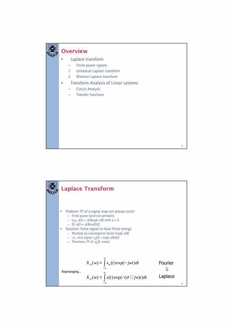
Laplace Transform
• Problem: FT of a signal may not always exist!– finite power (and not periodic), – e.g., x(t) = u(t)exp(-at)) with a < 0– Or x(t) = u(t)cos(5t)!
• Solution: Force signal to have finite energy– Multiply by convergence factor (exp(-σt))– i.e., new signal xσ(t) = exp(-σt)x(t)– Therefore, FT of xσ(t) exists
∫
∫∞
∞−
∞
∞−
+−=
−=
dttjwtxwX
dtjwttxwX
))(exp()()(
)exp()()(
σσ
σσ Fourier
Laplace
⇓Rearranging…
5
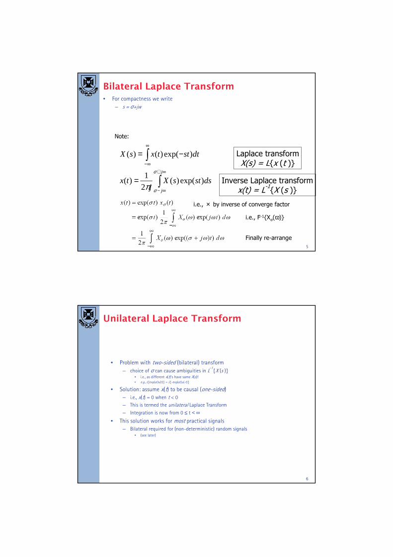
Bilateral Laplace Transform• For compactness we write
– s = σ+jw
∫
∫∞+
∞−
∞
∞−
=
−=
j
j
dsstsXj
tx
dtsttxsX
σ
σπ)exp()(
2
1)(
)exp()()( Laplace transformX(s) = L{x (t )}
Inverse Laplace transformx(t) = L
-1{X (s )}
Note:
i.e., F-1{Xσ(ω)}
i.e., × by inverse of converge factor
Finally re-arrange
6
Unilateral Laplace Transform
• Problem with two-sided (bilateral) transform
– choice of σ can cause ambiguities in L-1{X (s )}
• i.e., as different x(t)’s have same X(s)!• e.g., L{exp(at)u(t)} = L{-exp(at)u(-t)}
• Solution: assume x(t) to be causal (one-sided)– i.e., x(t) = 0 when t < 0
– This is termed the unilateral Laplace Transform
– Integration is now from 0 ≤ t < ∞• This solution works for most practical signals
– Bilateral required for (non-deterministic) random signals • (see later)

7
Unilateral Laplace Transform
• One-sided Laplace transform
• Laplace transform
– X(s) = L{x(t)}
• Inverse Laplace transform
– x(t) = L-1{X(s)}
∫∞
−
−=0
)exp()()( dtsttxsX
0- indicates origin is included in integration 0 ≤ t < ∞
8
Convergence of Laplace Transform
• Consider signal
• Convergence dependent on both σand a
– Note: ℜ{s} = σ• Region of Convergence (ROC)
– Finite integral (energy)
)()exp()( tuattx −=
a=-1
a=1a=2
( )( )[ ]
{ } asas
sX
ajwa
tasas
dtjwtta
dttassX
−>ℜ+
=
>+++
=
+−+−=
−+−=
+−=
∞
∞
∞
∫
∫
,1
)(
0,)(
1
exp1
)exp())(exp(
))(exp()(
0
0
0
σσ
σEffectively same as
� Fourier Transform
9
Laplace Examples
( ){ } ( ) ( )
( )
( )0,
1exp
exp
exp
0
0
0
>=
−−=
−=
−=
∞
∞
∞
∫
∫
σss
st
dtst
dtsttutuLUnit step function:
Impulse function: ( ){ } ( ) ( )
( ) ( )
( ) ( ) 10exp
exp
exp
0
0
0
0
=−=
−=
−=
∫
∫
∫
+
−
+
−
∞
∞−
dtts
dtstt
dtstttL
δ
δ
δδ
( ) ( ) ( ) ( ) ( ) ( ) ( )000
0
0
0
fdttfdtttfdtttf === ∫∫∫+
+
+
+
∞
∞−
δδδ
Remember:
10
Interpretation of Laplace Transform
• Represents signals, x(t), as sum of
– growing/decaying cosine waves
• at all frequencies (continuous), X(s)
– exp(σt )|X(s)|dw/2π is amplitude of growing/decaying cosine wave
• In frequency band w to w + dw
– ∠X(s) is phase shift of cosine wave
• parameter σ (ℜ{s}) determines rate of growth or decay
– Note: σ = 0 is the Fourier Transform ☺
• Constant amplitude cosine waves

11
Complex Phasors
Decaying σ < 0
Growing σ > 0
constant magnitude σ = 0As per Fourier Transform
12
Linear Transforms
• So far, we have looked at
– Fourier series
• Trigonometrical & Complex
– Fourier transform
– Laplace transform
• All represent signals as a
– Weighted sum (or integration) of
– Complex exponentials (that are orthogonal)
– e.g., complex FS, x(t) = Σ Xn exp(jnw0t)
• This relates directly to linear systems

13
Linear Transforms & Linear Systems
Useful, due to two properties of linear systems
1. Superposition principle
– Inputs are complex exponentials (sinusoids)
– Output is same exponentials, but with different weights, i.e., delay and amplify/attenuate input
( ) ( ){ } ( ){ } ( ){ }1 2 1 2H ax t bx t aH x t bH x t+ = +
In other words, each phasor can be considered individuallyand output calculated by summation of the individual phasors
14
Linear Transforms & Linear Systems
2. Ordinary differential equations (ODE)– Output y(t) related to input x(t) by ODE
m
m
mn
n
n dt
xdb
dt
dxbxb
dt
yda
dt
dyaya +++=+++ LL 1010
0 0 0
22
0 0 02
(exp( )) exp( )
(exp( )) ( ) exp( )
djn t jn jn t
dt
djn t jn jn t
dt
ω ω ω
ω ω ω
=
=
Differentiation is simple: • Frequency unchanged • Magnitude changes (complex)
Note: initially consider harmonically related sinusoids nω0 as per Fourier Series

15
Example RC Circuit
0 1 0 0
0
( ) exp( )
( ) exp( )
dya y t a b jn t
dtdy
y t RC jn tdt
ω
ω
+ =
+ =
x(t) (input)
R
C y(t) (output)
i
Specifically:a0 = 1 a1 = RCb0 = 1derivation shortly…
Using Kirchhoff’s laws, system described (modelled) by ODE
x(t) sinusoidal input(1 energy store ∴ 1st order)
16
Example RC Circuit
• If input single sinusoid xn(t) = exp(jnw0t)
– and system linear, (steady-state) output has form:
• Substituting (assumed) solution into ODE0( ) exp( )ny t K jn tω=
where K is complex constant (weight)
( ) ( )0 1 0 0 0
00
0 0 1
0
0
0 0 1 0
( ) ( ) exp
( ) exp( )( )
( ) exp( )
1
( ) 1 ( )
n n
n
n n
n
a y t a jn y t b jn t
by t jn t
a jn a
y t H jn t
bH
a jn a jn RC
ω ω
ωω
ω
ω ω
+ =
=+
=
= =+ +
Where Hn is the system transfer
function to thissingle phasor (K)
Same frequencyDifferent amp. &/or phase
( ) ( ) ( )0n
n
dy tjn y t
dxω=Note:

17
Response of Linear System
• Input represented as Fourier series
X1exp(jw0t)
X2exp(j2w0t)
Xnexp(jnw0t)
Σ Linear Systemy(t) x(t)
18
Response of Linear System
• Applying superposition principle– Applying individual phasors & shifting Xn terms
Σ
X1
H1 exp(jw0t)Linear System
y(t)
X2
H2 exp(j2w0t)Linear System
Xn
Hn exp(jnw0t)Linear System
exp(jw0t)
exp(j2w0t)
exp(jnw0t)
Each phasor is orthogonal and ∴ can be evaluated separately

19
Response of Linear System
• Output represented as Fourier series– output FS coefficients Yn = Hn Xn
Σ y(t)
H1X1exp(jw0t)
H2X2exp(j2w0t)
HnXnexp(jnw0t)∑
∞
−∞=
=n
nn tjnwXHty )exp()( 0
Input |.| & ∠ at this frequency
System |.| & ∠ at this frequency
Output |.| & ∠ at this frequency
20
General Approach
• Represent input as weighted sum of – Complex exponential basis functionsbasis functionsbasis functionsbasis functions,
– e.g., FS: exp(jnω0t): sinusoids at harmonic frequencies
• Basis functions are orthogonal– Amplitude (& phase) at each freq. evaluated separately
• System described by ODE– Response to exponentials (differentials) easy to calculate
• Frequency remains constant, Amp. & Phase change
– e.g., if response 2nd harmonic is 2ω0exp(2jω0)
• System is linear– Output is sum of responses of individual exponentials
• i.e., sum response at each frequency

21
Laplace Transforms
• General approach was illustrated with
– Periodic input (i.e., we used Fourier series)
– Steady state response
• But, in general interested in
– non-periodic input and
– Both transient & steady state response
• So, we use the Laplace transform
– Basis functions exp(st), where s = σ+jw– output response is H(s) exp(st)
– where H(s) is system transfer functiontransfer functiontransfer functiontransfer functionNote: still orthogonal
22
Laplace System Analysis
Steps in Laplace system Analysis,
1. Laplace transform input signal– X(s) = L{x(t)}
2. Calculate system transfer function– H(s)
3. Calculate (Laplace) output using multiplication– Y(s) = H(s)X(s)
4. Inverse Laplace transform– y(t) = L-1 {Y(s)}
Key: Calculating system transfer function: H(s)
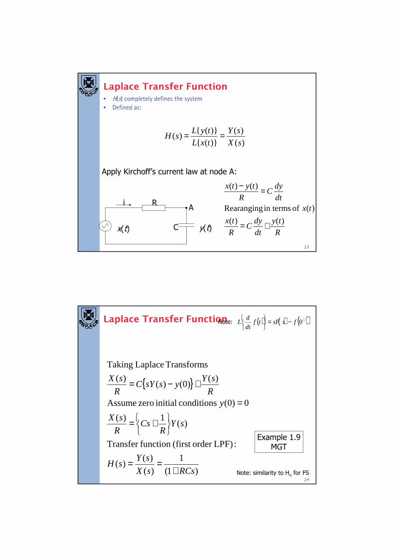
23
Laplace Transfer Function• H(s) completely defines the system
• Defined as:
)(
)(
)}({
)}({)(
sX
sY
txL
tyLsH ==
R
ty
dt
dyC
R
tx
txdt
dyC
R
tytx
)()(
)( of in terms Rearanging
)()(
+=
=−
x(t)
R
C y(t)
iA
Apply Kirchoff’s current law at node A:
24
Laplace Transfer Function
{ }
)1(
1
)(
)()(
:LPF)order (first function Transfer
)(1)(
0)0( conditions initial zero Assume
)()0()(
)(
Transforms Laplace Taking
RCssX
sYsH
sYR
CsR
sX
yR
sYyssYC
R
sX
+==
+=
=
+−=
Example 1.9MGT
( ) ( ) ( )+−=
0fssFtf
dt
dLNote:
Note: similarity to Hn for FS

25
Laplace Circuit Analysis
• Transform circuit elements– then apply Kirchoff’s current law
• Impedance of Capacitor = 1/Cs
– (Note: impedance of inductor = Ls)
X(s)
R
1/Cs Y(s)
A
)1(
1)(
)(1
)()()(
RCssH
sCsYCs
sY
R
sYsX
+=
==−
This is quick and easy way of doing circuit analysis
26
Laplace Circuit Analysis
• Impedance of Inductor = Ls
X(s)
R
Ls Y(s)
A
)()1(
1)(
)(1)()(
)(1)()(
RLs
Ls
Ls
RsH
sYsLR
sYsX
dttyLR
tytx
+=
+=
=−
=−∫By Kirchoff’s current law:
First order HPF
( ) ( )s
sFdfL
t
=
∫0
ξξNote:
27
Summary
• Laplace transform similar to Fourier– Applicable to broad range of signals
– Most one-sided (causal) finite energy and power
• Particularly useful for– solving ODE’s i.e., analysing linear, time-invariant systems (e.g., circuit
analysis)
• Based on summation (integration) of– (orthogonal) exponential (basis) functions
• like Fourier series and transform
– System response scaled versions of these• amplitude and phase change (only) at each frequency