Elasticity of Supply to the Firm and the Business Cycle · PDF fileElasticity of Supply to the...
40
Elasticity of Supply to the Firm and the Business Cycle Briggs Depew University of Arizona Todd A. Sørensen University of California, Riverside IZA August 23, 2011 Abstract A body of recent empirical work has found strong evidence that the labor elasticity of supply to the firm is finite, implying that firms may have wage setting power. However, these studies capture only snapshots of the parameter. We study this parameter over a period that provides substantial variation in the business cycle. Using a rich employee level dataset from the inter-war period, we are able to estimate the elasticity of supply to the firm during several recessions and expansions. Our analysis suggests that the elasticity is indeed lower during recessions, consistent with the comparative statics from the Burdett-Mortensen search model. This differential wage setting power over the business cycle provides an alternative explanation of the pro-cyclicality of wages. Contact Todd Sorensen at [email protected] and Briggs Depew at [email protected]. Feedback received at The University of Arizona, Dalhousie University, Konstanz University, and Lund University is greatly appreciated. Todd Sorensen is grateful to ROA Maastricht University where part of this research was conducted during a sabbatical visit. Alyssa Depew, Arindrajit Dube, Bryan Engelhardt, Torberg Falch, David Farris, Price Fishback, Taylor Jaworski, Ryan Johnson, Alan Manning, Mindy Marks, Ronald Oaxaca, Kathryn Radzik, Michael Ransom, Michael Reich, Chad Sparber, and Mo Xiao provided helpful feedback. Thanks to Kelvin Zhang Yi and Eric Siyu Lu for their research assistance. 1
Transcript of Elasticity of Supply to the Firm and the Business Cycle · PDF fileElasticity of Supply to the...

Elasticity of Supply to the Firm and the Business Cycle
Briggs DepewUniversity of Arizona
Todd A. SørensenUniversity of California, Riverside
IZA
August 23, 2011
Abstract
A body of recent empirical work has found strong evidence that the labor elasticity of supplyto the firm is finite, implying that firms may have wage setting power. However, these studiescapture only snapshots of the parameter. We study this parameter over a period that providessubstantial variation in the business cycle. Using a rich employee level dataset from the inter-warperiod, we are able to estimate the elasticity of supply to the firm during several recessions andexpansions. Our analysis suggests that the elasticity is indeed lower during recessions, consistentwith the comparative statics from the Burdett-Mortensen search model. This differential wagesetting power over the business cycle provides an alternative explanation of the pro-cyclicalityof wages.
Contact Todd Sorensen at [email protected] and Briggs Depew at [email protected] received at The University of Arizona, Dalhousie University, Konstanz University, andLund University is greatly appreciated. Todd Sorensen is grateful to ROA Maastricht Universitywhere part of this research was conducted during a sabbatical visit. Alyssa Depew, Arindrajit Dube,Bryan Engelhardt, Torberg Falch, David Farris, Price Fishback, Taylor Jaworski, Ryan Johnson,Alan Manning, Mindy Marks, Ronald Oaxaca, Kathryn Radzik, Michael Ransom, Michael Reich,Chad Sparber, and Mo Xiao provided helpful feedback. Thanks to Kelvin Zhang Yi and Eric SiyuLu for their research assistance.
1

1 Introduction
One of the most important, yet understudied, parameters of the labor market is the elasticity of
labor supply to the firm. A finite elasticity of supply may contradict the classic assumption that
firms have no wage setting power. If firms face no other constraints in setting wages, the finite
elasticity will drive a wedge between a worker’s wage and her marginal revenue product. Manning
(2003) posits that labor market frictions imply that a model with upward sloping supply curves to
the firm, as first described by Robinson (1933), best represents the labor market.1 Ultimately, the
value of the elasticity of supply to the firm is an empirical question. A small but quickly growing
literature has attempted to estimate this parameter.2
All previous work has captured only snapshots of this elasticity. Our primary contribution is
to study how this elasticity varies over the business cycle. We show that the Burdett-Mortensen
search model predicts pro-cyclicality in the elasticity of supply to the firm. This implies that firms
may have more wage setting power during recessions than during expansions. This is consistent
with empirical evidence of the pro-cyclicality of wages, but provides a different theoretical basis
than has been offered in the past: differential wage setting ability over the business cycle.
To test for the cyclicality of this parameter, we employ a rich dataset of employee records from
the Ford Motor Company for the inter-war years of 1919 through 1940 (Whatley and Wright 1995).
From this data, Whatley and Sedo (1998) and Foote, Whatley and Wright (2003) suggest that
Ford may have enjoyed monopsony power during this period, but do not estimate the supply elas-
ticity directly. This data covers five NBER defined contractions and six NBER defined expansions
(Committee 2011). The highly volatile labor market during this period provides us with the vari-
ation needed in the business cycle to identify the cyclicality of the elasticity of supply to the firm.
No other twenty year period provides us with the same frequency and degree of business cycle
variation. Our primary finding is that the elasticity of supply to the firm, never more than six in1For a more detailed summary of monopsonistic labor markets see Ransom (1993) and Boal and Ransom (1997)2See Boal (1995), Ransom and Oaxaca (2005), Ransom and Oaxaca (2010), Hirsch, Shank and Schnabel (2006),
Hirsch (2007), Hotchkiss and Quispe-Agnoli (2009), Ransom and Sims (2009), Ransom and Lambson (2011), Hirsch,Shank and Schnabel (2010), Falch (2010), and Falch (2011). Many of these estimates are in the range of 1 to 3.Dube, Lester and Reich (2011) estimate structural parameters of the Burdett-Mortensen search model using reducedform supply elasticities resulting from exogenous variation in minimum wages and find estimates in the 4 to 10 range.Staiger, Spetz and Phibbs (2010) use an exogenous wage change and find a short-run elasticity of supply of 0.1.
2
any period, drops by around half in a recession. Lack of an instrumental variable likely biases our
point estimates of the elasticity downward. However, we show that we are likely underestimating
the cyclicality of the elasticity as estimates are more biased during periods of economic growth
than during periods of contraction, thus strengthening our results regarding the cyclicality of the
parameter.
Our work also contributes to the literature on the identification of the labor elasticity of supply
to the firm. First, our identification strategy extends the standard methodology by relaxing the
assumption that the firm replaces all separations with recruits. This strategy is necessary because
our study involves a long period of time involving large fluctuations in employment. It will also
prove useful as a more robust estimation strategy for future researchers. Second, our rich-firm level
data allows our empirical analysis to more closely follow the theoretical model than prior studies.
Specifically, we document that a downward bias occurs when separation elasticities are calculated
using both voluntary and involuntary separations, as has been done in the past.
3
2 Model and Empirical Strategy
We extend the standard model used to estimate labor supply elasticities to the firm to take into
account fluctuations in the business cycle. Our extension is applicable for firms that are expand-
ing or contracting employment. This allows us to credibly estimate how εLw changes over the
business cycle. We also present a simplified Burdett and Mortensen (1998) search model that pro-
vides the theoretical foundation for the dynamic monopsony setting. We derive predictions of how
macroeconomic shocks cause changes in εLw through changes in the structural parameters of the
model.
2.1 Estimating Labor Elasticity of Supply to the Firm
Manning’s (2003) dynamic model of monopsony provides the foundation for the estimation approach
used in this paper. The model makes use of an assumption of a steady state in employment and an
insight from Card and Krueger (1995) which provides a method for obtaining the long-run supply
elasticities to the firm. From Card and Krueger (1995) the elasticity of supply to the firm is
εLw = εR − εs, (1)
where εR is the recruitment elasticity and εs is the separation elasticity. When a firm is neither
expanding nor contracting in employment, i.e. employment is in a steady state, Manning (2003)
shows that εs = −εR. This identity is derived from the fact that workers in the same labor market
face a similar job offer arrival rate, λ, and wage offer distribution, F (·). One can then simply apply
the identity from Card and Krueger (1995) to show that εLw = −2εs. This identity has been used
in most previous work measuring εLw, because separations are much easier to observe in data than
are recruits. Thus, other studies implement a strategy estimating εs and then calculating εLw as -2
times εs.
As the goal of this paper is to understand how the labor elasticity of supply to the firm, εLw,
varies over the business cycle, we must consider how to calculate εLw when the firm’s employment
levels are not constant. To the best of our knowledge, prior work has not developed an estimation
4

strategy robust to growth or contraction in employment at the firm.
We find that the generalized relationship between εLw and εs is
εLw = −(1 + γ)εss(w)
1− [1− s(w)]γ, (2)
where γ is the inverse employment growth rate during the period and s(w) is the separation rate.
Note that when γ = 1, the elasticity of labor supply to the firm, εLw, is simply equal to the result
given above: εLw = −2εsw. The derivation of equation 2 is found in the appendix.
It is easy to see that if γ 6= 1, an incorrect assumption of constant employment between time
periods will generate a biased result. If the firm is expanding (γ < 1), εLw will be overestimated,
and if the firm is contracting (γ > 1), εLw will be underestimated. This is important as we study
how εLw changes over the business cycle so that we do not over estimate the elasticity during
expansion and under estimate it during contraction.
2.2 Pro-cyclicality in the Labor Elasticity of Supply to the Firm
Here we show how changes in two key structural parameters of the Burdett-Mortensen search model
(the job offer arrival rate and the job destruction rate) affect the elasticity of supply to the firm. As
would be expected, a higher rate of job arrivals and a lower rate of job destruction decrease frictions
in the labor market and decrease attachment to a particular firm. In sum, the Burdett-Mortensen
search model tells us that εs will be counter-cyclical and thus εLw will be pro-cyclical.
In the Burdett-Mortensen model, the separation rate of employees at a firm, s(w), is defined by
s(w) = δ + λ[1− F (w)], (3)
where δ is the job destruction rate, or the rate at which employed workers exit the firm for non-
employment, λ is the job offer arrival rate, and F (w) is the probability that a wage offer dominates
the current wage. The separation elasticity is therefore defined as
εs = −ws′(w)
s(w)=
−λf(w)wδ + λ[1− F (w)]
. (4)
5
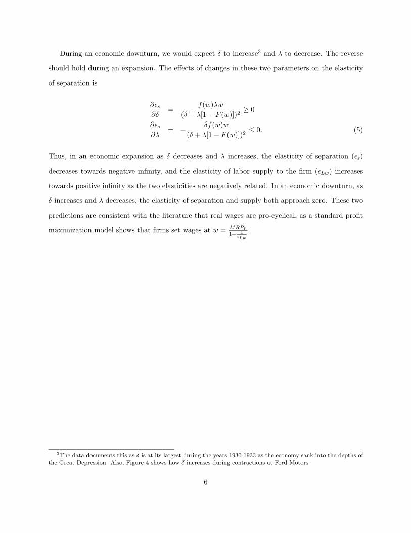
During an economic downturn, we would expect δ to increase3 and λ to decrease. The reverse
should hold during an expansion. The effects of changes in these two parameters on the elasticity
of separation is
∂εs∂δ
=f(w)λw
(δ + λ[1− F (w)])2≥ 0
∂εs∂λ
= − δf(w)w(δ + λ[1− F (w)])2
≤ 0. (5)
Thus, in an economic expansion as δ decreases and λ increases, the elasticity of separation (εs)
decreases towards negative infinity, and the elasticity of labor supply to the firm (εLw) increases
towards positive infinity as the two elasticities are negatively related. In an economic downturn, as
δ increases and λ decreases, the elasticity of separation and supply both approach zero. These two
predictions are consistent with the literature that real wages are pro-cyclical, as a standard profit
maximization model shows that firms set wages at w = MRPL1+ 1
εLw
.
3The data documents this as δ is at its largest during the years 1930-1933 as the economy sank into the depths ofthe Great Depression. Also, Figure 4 shows how δ increases during contractions at Ford Motors.
6

3 Data
The data for this paper is extracted from a larger dataset covering a sample of employee records
at Ford Motors from 1918 to 1947. The data’s principal investigators, Warren Whatley and Gavin
Wright, obtained employee work history through random sampling of archived records (Whatley
and Wright 1995). Maloney and Whatley (1995) begin to convey the idea that Ford Motors may
have had potential monopsony power over its workers. Later work by Whatley and Sedo (1998)
studies the quit behavior of workers at Ford Motors. Although the labor supply parameters that
are the focus of our paper are not estimated, their work did recognize potential monopsony power.
They state that, “the additional monopsony power that employers have over black workers results
in poorer job matches for black workers and lower reservation utilities. A lower reservation utility
reduces job search and the propensity to quit.” Foote et al. (2003) extends the work of Whatley
and Sedo (1998) and also suggests the existence of monopsony power.
The data was obtained in such a way that only workers who had separated from Ford Motors
by 1947 were intended to be included in the sample. Therefore, observations of workers with hire
dates closer to 1947 are fundamentally different from those in earlier time periods. Observations
for these workers had shorter tenure spans by construction of the sample. We limit our sample to
pre-1941 data not only because of this sample selection bias, but also because Ford Motors became
unionized in 1941 and the industrial landscape began to change due to the war. Observations from
1918 may have also been affected by policies related to World War I and are thus also omitted.
Each worker in the original sample is identified by a unique ID. When a job characteristic such
as wage or job position changes, a new job record was recorded. Included in the job record is a
variable that indicates when the job ended and whether the person moved internally in the firm,
such as to a new position or even a new wage, or whether the move was external through quitting,
being fired, being laid-off, military leave, etc.
In order to estimate the labor elasticity of supply to the firm, we needed the data to be structured
into equal length periods. We follow an estimation approach similar to Ransom and Oaxaca (2010),
who used year-end payroll data of a firm. We use the original Ford Motor employee data to
create semi-annual observations of employment status, wages, and tenure. We chose semi-annual
7
observations rather than annual observations because the average time between a wage change for
an employee was typically between five to six months, as reported in Table 2.4 Having finer time
periods also allows us to more precisely estimate the cyclicality of the labor elasticity of supply to
the firm.
The employee records provided the specific job title of each employee. However, these job titles
were not systematically organized. To capture the causal effect of wages on separation, one needs
to control for jobs or tasks that may be correlated with wages and that also affect an employee’s
decision to separate from the firm, for example, compensating wage differentials for working in
undesirable jobs. We use the job titles from the data to create job-specific indicator variables. We
found the most commonly used words to describe a job position and matched it with a corresponding
indicator variable.5
Summary statistics for the Ford data are given in Table 1. Each observation in the table
is a semi-annual worker observation as used in the analysis section. Table 2 provides detailed
information on separations and nominal wage changes at Ford. Involuntary separations were not
a trivial share of total separations in any time period. The number of nominal wage changes was
dominated by upward changes. However, there were downward changes in wages in each period.
From the second of 1929 through the first half of 1933, 35% of wage changes were downward.
We also obtained average and peak employment data from Ford’s archive to calculate year
to year growth rates during this period(Archives 1903-1972). Data on growth rates is needed to
correctly adjust the elasticities when a firm’s employment levels are not constant over time. Figure
1 shows both average and peak employment over the period of study.
4There is no consensus in the literature on the frequency of data to be used. Ransom and Oaxaca (2010) useyearly observations while Hotchkiss and Quispe-Agnoli (2009) use monthly observations. Intuitively, the length oftime used should coincide with the employees’ decisions to separate. Since we are interested in how wages affectseparation decisions it seems appropriate to equate the length of the time period to the average time between wagechanges. Also, as we are interested in changes in the parameter over the business cycle, our final results should beinvariant to specification choices uniformly affecting the level of the parameter in different time periods, as a differentchoice of time frame may do.
5We chose to aggregate to the following ten job titles: assembly, operator, laborer, maker, gdr, trade, hand, upper,missing, and other. The “trade” job title refers to jobs such as welding and electrician. The title “hand” refers tojobs such as machine hand or press hand. “Upper” workers are in reference to clerks, inspectors, and foreman. Theabbreviation “gdr” is unknown but commonly used.
8

4 Estimation Strategy and Identification
As shown previously, the elasticity of labor supply to a firm can be identified through the elasticity
of separation. Between the years 1919-1940, Ford Motors was often expanding or contracting in
employment. Manning’s (2003) assumption that the firm’s employment level is in a steady state
can be relaxed if one knows the growth rates of the firm over the time period and applies the
methods in Section 2. Here we explain how we will estimate the separation elasticities and then
solve for the labor elasticity of supply to Ford Motors.
4.1 Estimation Strategy
We use a linear probability model (LPM) to estimate the elasticity of separation with respect to
wage,6
si = β0 + β1 ln(wi) +XiB + µi, (6)
where si is the binary variable indicating that individual i separated from their job at Ford Motors
by voluntarily quitting. wi is the wage of individual i and the vector Xi represents other observable
variables for each individual that affect the separation decision. Included in Xi are age, job tenure,
age and job tenure squared, race, marital status, job, plant, and year fixed effects. µi is a vector of
unobserved variables.
We estimate four specifications of the LPM. The first specification excludes all controls except
for year fixed effects which control for the price level. The second specification adds the individual
level control covariates into the model. Controlling for actual experience at Ford is important, as
we are trying to isolate the effect of wages on the decision to separate. Without controlling for this
the true effect of wages on separation is confounded by more tenured workers receiving higher wages
and being more attached to the firm because of other reasons. The third and fourth specifications
add plant and job title fixed effects, respectively. Plant fixed effects control for working conditions,
which varied across plants (Foote et al. 2003). The job titles are used to control for unobserved6We also estimated the elasticities with a Probit model and found similar results. The choice to use the LPM over
the Probit model mainly resulted from the ease in bootstrapping the standard errors. The Probit specification ismuch more sensitive than the LPM specification when bootstrapping over smaller samples. However, point estimatesand statistical significance were similar between the two models when there was a relatively large sample.
9

tasks that were required of workers. Controlling for job titles and race is important in light of the
evidence in Foote et al. (2003) showing that black workers were often placed into more dangerous
and less desirable jobs than white workers.
The separation elasticity for each individual i is calculated from the linear regression model in
the following way,
εs,i =∂si∂wi
wisi
=β1
β0 + β1 ln(wi) +XiB. (7)
A point estimate of εLw was calculated by first solving for the average separation elasticity, εs =
1N
∑i εs,i, then applying equation 2 from Section 2.
Figure 1 shows the trends in average and peak employment at Ford Motors over our period of
study.7 Period specific γ’s were obtained from the year level data seen in the figure. From 1919
through 1929 employment, for the most part, steadily increased; this is consistent with the general
growth of the U.S. economy. Ford Motors experienced a large-scale contraction along with the U.S.
economy between 1929 and 1933. Growth once again picked up in 1933.
Given these different economic conditions over the time period of study, we begin our analysis
of the variation in εLw by estimating the value of the parameter for each of the following three
major sub-periods: 1) 1919 through the first half of 1929 (“The Roaring Twenties”), 2) the end of
1929 through the first half of 1933 (“The Great Contraction”), and 3) the period from the second
half of 1933 through 1940 (“The New Deal”).
We next turn our attention to the NBER defined expansions and contractions during our period
of study. No other 22-year period in the United States during the 20th century observed such large
and frequent fluctuations in the business cycle. We partition the data into 11 sub-periods for each
expansion (6) and contraction (5) in the period of study. We then estimate the elasticity of supply
to the firm for each sub-period.
4.2 Identification
Causal identification of the elasticity of separation is the first step in the identification of εLw.
To consistently identify the elasticity of separation, we must have variation in wages which is7The data was obtained from the Ford Motor archives through personal request (Archives 1903-1972).
10

independent from other unobserved factors that affect the probability of separating. Our wage
variation comes from different workers being paid different wages after conditioning on job title,
plant location, year, tenure, and other demographic information. Even with this rich set of controls,
we acknowledge the potential for omitted variable bias. Below we discuss the instrumental variable
approaches that have been undertaken by a small number of papers in this literature, then we
attempt to sign the bias that may affect our estimates.
Ransom and Sims (2009) is able to identify the elasticity of separation by instrumenting actual
salaries with pre-negotiated salaries for school teachers. Similarly, Falch (2011) was able to exploit
an exogenous wage change for a subset of school teachers. Ransom and Sims (2009) finds that
without instrumental variables, the elasticity of separation is biased upward and as a result the
labor elasticity of supply to the firm is biased downward. Other recent papers in this literature
that have analyzed private sector data, like ours, have not been able to find a valid instrument to
overcome endogeneity issues.8
Following the linear specification described above, suppose µi can be decomposed as τyi + ξi.
Therefore, the equation of interest is,
si = β0 + β1 ln(wi) +Xiβ2 + τyi + ξi, (8)
where yi represents an unobserved variable that is correlated with ln(wi) and ξi represents a vector
of unobserved characteristics such that E[ξi|ln(wi), Xi, yi] = 0. As long as τ 6= 0, the parameter of
interest, β1 cannot be estimated consistently:
plim β1 = β1 + τθ, (9)
where θ is the coefficient on ln(w) in the population regression of the omitted variable, y, on ln(w)8To properly instrument for wages we need an instrument that is correlated with wages, does not directly affect
separation decisions, and varies across individual employees. An ideal instrument would be a mechanism that ran-domly assigns wages to individual employees. Uncovering such an instrument in this context is difficult to imagine.Dube et al. (2011) is able to account for interactions among firms and workers in their estimation. Such equilib-rium effects are important as identification comes through changes in the minimum wage which in turn affects thewage distribution of all firms. Our identification comes through variation in wages at Ford alone. However, outsidefirm-employee interactions are still a concern as we describe later in the section.
11

and X.
The potential endogeneity issue that arises in our study is the concern that outside labor demand
shocks, yi, faced by individual i are positively correlated with wages after controlling for individual
characteristics as well as year, plant and job title fixed effects.9 Therefore, θ is positive. Likewise,
τ is believed to be positive as outside positive demand shocks for labor increase the job offer arrival
rate, λ, and the probability of separating from the firm. With τθ > 0, the estimated coefficient
on ln(w), β1, is biased in a positive direction. Therefore, εs would also be biased in a positive
direction, which would cause εLw to be biased in a negative direction.
However, we expect that θ is not constant over the business cycle. Specifically, wages are
typically more sticky downward than upward. Table 2 shows wage changes at Ford Motors over
time. Although, we see variation in both directions, wages move upward more easily in periods
with high outside labor demand than they move downward during periods of low outside labor
demand. These movements suggest that the magnitude of the bias, τθ, is not constant because
θ is greater during times of economic expansion than during times of economic contraction. The
greater downward bias during expansions implies that our estimate of the difference in the elasticity
between expansions and contractions will also be biased downwards. Thus we will underestimate
the pro-cyclicality of the elasticity of labor supply to the firm.
4.3 Estimation Bias from Involuntary Separations
The underlying idea in the search framework is that individuals voluntarily separate because they
accept a higher wage elsewhere (Manning 2003). Therefore, identification of εLw should come
from seeing how wages and voluntary separations covary. The data used in previous empirical
work has not specified the reason for separation, which creates measurement error problems. The
Ford employee data specifies whether the separation was a voluntary quit or a forced lay-off or9We also experimented with including peer variables that may be correlated with log wages and plausibly correlated
with unobserved labor demand shocks. The three peer variables included in the estimation equation are the averagewage of workers with the same tenure, workers in the same job title, and workers in the same plant. It is possiblethat individuals make wage comparisons between themselves and their peers when determining quitting decisions.However, the key idea behind the peer variables is to proxy for labor demand shocks at the individual level in orderto minimize the endogeneity of wages. However, the estimated results were robust to the inclusion of these peervariables.
12

firing. Therefore, we are in the position to eliminate and assess the potential bias due to the
misclassification of reasons for separating.
The bias is not straightforwardly signed when both voluntary and involuntary separations are
used to estimate population parameter on ln(w), β. In the extreme case, suppose that involuntary
separations, s′i, are orthogonal to log wages. Therefore, the estimate of β, using both voluntary and
involuntary separations, is biased towards zero as it is a weighted average of zero and β. However,
it is not clear that log wages are orthogonal to involuntary separations. One possibility is that
log wages and involuntary separations are negatively correlated even after controlling for Xi. We
address the direction of this bias empirically in the next section by comparing point estimates of
the elasticity of supply to the firm under inclusion and exclusion of involuntary quits. Furthermore,
we separately analyze the correlation between wages and fires and layoffs.
13

5 Results and Discussion
5.1 Main Results
Results from a set of linear probability model estimations using all years of data are presented
in Table 3. In each estimation, we find a negative and statistically significant coefficient on log
wage. The relatively small magnitudes of these coefficients suggest that a finite elasticity of labor
supply to the firm is expected. The first specification includes only year fixed effects. In the second
specification, we control for individual covariates. The linear tenure term is always negative and
significant, while age is positively correlated with separations. Marital status has a marginally
significant and positive effect on separations. The coefficient on an indicator variable for African-
American workers is negative and always significant (consistent with Foote et al. (2003)). The
third and fourth specifications include additional fixed effects for the plant at which the worker was
employed and the worker’s job title, respectively. The results are similar to the second specification
and suggest robustness in our results after conditioning on key demographic variables.
In Table 4, we report the labor elasticity of supply to the firm (εLw) from the estimation strategy
outlined in Section 2 and 4, which incorporates γ. The standard errors on the elasticity estimates
are obtained by bootstrapping with 500 replications.10 Estimates of the elasticity obtained from
pooling all years range from 3.03 to 3.88. The estimates from three major sub-periods are also
reported in Table 4.11 Across all four specifications we note a similar pattern. First, the estimate
of the labor elasticity of supply to the firm in The Roaring Twenties is similar in magnitude to the
estimate in the pooled sample (because a large fraction of observations come from those years).
Second, the estimate of the labor supply elasticity falls sharply during the Great Contraction. This
result is consistent with the finding of Bresnahan and Raff (1991), that show from the peak of
1929 to the trough of 1933, half of the U.S. auto plants shut down while only one third of U.S.10To obtain the bootstrapped standard errors, we used the bootstrapping package provided by Stata. This package
called a program from which an LMP was run and the supply elasticity was calculated post-estimation. We then foundthe standard deviation of the distribution of all 500 estimates of the elasticity provided, including from estimatesin which not all parameters or their standard could be estimated. We presume that some parameters could not beestimated in every bootstrapped sub-sample on account of the high number of fixed effects in the full model combinedwith the relatively small sample size in some of the sub-periods.
11In the appendix we report the estimates of the linear probability model run for the preferred fourth specificationfor each of the three major sub-periods. The full set of results is available upon request from the authors.
14

manufacturing establishments were closed. Therefore, job specific capital that Ford workers had
would have been relatively less demanded. Thus, the decrease in the elasticity of supply is due to this
decrease in the job offer arrival rate (λ). None of our point estimates from The Great Contraction
are significantly different from 0, thus we cannot reject a null hypothesis of perfectly inelastic
labor supply to the firm during this period.12 Finally, during the recovery period beginning after
1933, the labor supply elasticity increases to levels comparable to those of the Roaring Twenties.
Elasticities during the New Deal were slightly higher than during the Roaring Twenties, suggestive
of the effects of various changes to the labor market enacted during the New Deal.13
The results in Table 4 are prima facia evidence of the pro-cyclicality of the elasticity of labor
supply to the firm: the elasticity plummeted as the country sank into the Great Depression, and
then increased in value as the economy began to recover. We now further examine this relationship
using finer sub-periods in time from our data. First, in Figure 2 we present estimates of the
elasticity obtained from pooling data into three period windows.14 The figure also plots the national
unemployment rate.15 We see more evidence consistent with pro-cyclicality of the elasticity: the
large increase in unemployment beginning after 1929 is consistent with the plummeting elasticities
during this period. While the persistently high unemployment of the mid 1930s is not consistent
with the increasing elasticity during the same time, we do see the unemployment rate start to
decrease in 1934, around the time the elasticity of supply starts to increase.12While we would expect that the economic conditions during this period would create very inelastic labor supply,
we also believe that our estimates tend to be biased downwards for reasons as noted previously. Ransom andSims (2009) find that estimates of the elasticity of supply to the firm are biased downward prior to implementinginstrumental variables. This is consistent with Falch (2010) who finds downward bias through omitted variables.
13The Wagner Act of 1935 expanded employee collective bargaining rights and resultantly union membership rose.While Ford did not unionize until 1941, General Motors and Chrysler unionized during the mid 1930s. As unioncontracts increased wages significantly (we see this in our data from Ford when comparing 1940 and 1941), this likelyshifted the wage offer distribution to the right for Ford workers (as GM and Chrysler’s wages increased more quicklythan Ford’s.) The Fair Labor Standards Act of 1938 set a national minimum wage and overtime requirements. TheFederal Emergency Relief Administration, the Civil Works Administration, and the Works Progress Administration,all created in the New Deal era, offered government sponsored work relief on a large scale. These would have theeffect of increasing the job arrival rate during this period. Social insurance programs were created through the SocialSecurity Act of 1935. Such reform likely impacted the reservation wage of workers. See Fishback (2008) for a moredetailed summary of New Deal policies.
14To make the scale of the figure more concise, we bound the elasticity at its theoretical lower bound of 0. Theapproximate values of the parameter not shown above are as follows for each window centered around the given year:1931(I) is -3.7, 1931(II) is -6.7, 1932(I) is -4.9, 1932(II) is -6.0, 1933(I) is -1.2.
15Source of unemployment data is drawn from Romer (1986) and Coen (1973) as compiled by athttp://en.wikipedia.org/wiki/User talk:Peace01234 .
15

A cleaner test for the pro-cyclicality of the elasticity requires a sharper definition of the state of
the economy. Therefore, we turn to NBER business cycle data that defines peak and trough dates
of the business cycles throughout the 1920s and 1930s in order to directly test whether recessions
decrease the labor elasticity of supply to the firm. Figure 3 presents the 11 NBER defined sub-
periods and the estimates of the labor elasticity of supply to the firm in each sub-period.16 Six
blue dots represent estimates obtained during periods of expansion, while five red dots represent
estimates obtained during recessions. The size of each dot is proportional to the number of years
represented. With the exception of the first recessionary sub-periods, we see that whenever the
economy fell into recession, our estimate of the elasticity was lower than in the expansions that
preceded and followed the recession.17 This data is also presented in Table 5. Arrows indicate the
direction of the economy in the period. Note that with the lower elasticities in recessionary periods
also come higher markdown rates.18
Finally, in Table 6 we present the results of tests for the pro-cyclicality of the elasticity of labor
supply to the firm using the data presented in Table 5 and Figure 3. We regress both the level of
the elasticity and changes in the elasticity on an indicator variable for a recessionary sub-period.
Additionally, we perform non-parametric tests of a null hypothesis that the estimated elasticities
during expansions and contractions resulted from the same data generating process.
We run three parametric regressions on each dependent variable; these differ according to re-
gression weights used. Regardless of the weights, all 6 regressions yield negative coefficients varying
between -1.12 and -5.09, indicating the economic significance of a recession on the elasticity of labor
supply to the firm. Our first weighting strategy is to weight by the inverse of the standard error
on the point estimate of the elasticity in the sub-period. Thus, when using this weight, we put
more weight on periods for which we have a more precise estimate. Our second weighting strategy
is to weight proportionately to the number of years covered in each sub-period. This weight allows
the model to put more weight on longer expansions or contractions. This may be appropriate for16We define a semi-annual period as being part of an expansion/recession if more than half of the period was in an
NBER defined expansion/recession.17We present this same figure with the supply elasticities calculated by multiplying the separation elasticity by
negative two in Appendix Figure 1. This evidence points more strongly towards pro-cyclicality of the parameter.18The potential markdown is defined as MRPL−w
MRPLand was equated through the identity that the rate of potential
employee exploitation is equal to the inverse of εLw.
16

two reasons. If we consider an observation to be a recession or an expansion, this weighting is not
necessary. But if we consider an observation to be a time period in a given economy, we should
put more weight on longer expansions and contractions than on shorter ones. Second, a recession
may require some persistence in order to affect the elasticity of supply to the firm. This weighting
strategy would capture the effects of persistence. Finally, we weight by the product of both of the
weights described above, addressing both of the issues discussed here simultaneously.
We find negative but insignificant results when weighting by the inverse of the standard errors
for both of the dependent variables. However, when we weight by period length, we find negative
results that are significant at the 5% level for the elasticity level and 10% level for changes in
the elasticity. Finally, when weighting by the product of the two earlier weights, we find negative
and marginally significant results. Our non-parametric test is a Mann-Whitney “ranksum” test.
The null hypothesis is that elasticity estimates for both the recession and expansion periods were
generated by the same data generating process. We are able to reject the null at the 0.0001 level.
This rejection implies that the data generating process for recessionary periods produced lower
elasticities of supply.
Together, these results confirm the comparative statics derived from the Burrdett-Mortensen
model and presented in Section 3, namely that the labor elasticity of supply to the firm is pro-
cyclical. Potential downward estimation bias of the elasticity is larger during periods of economic
growth. Therefore, endogeneity issues bias us against finding a result.
5.2 Additional Estimation Issues
5.2.1 Employment Adjustment and Voluntary Quits
Here we address the importance of adjusting for changes in the employment level over time and
using only voluntary quits to estimate εLw. To examine the potential bias we 1) re-estimated the
model without adjusting for changes in the employment level and using only voluntary quits, and
2) re-estimated the model where we adjust for employment changes but include both voluntary
and involuntary separations in the analysis. The results in Table 8 are estimated from specification
four, which included individual controls as well as year, plant, and job title fixed effects. Both
17

types of specification error impact the estimates of εLw.
If the firm is expanding employment and we use the traditional approach of setting εLw = −2εs
then the εLw is over-estimated. Similarly, if the firm’s employment level is decreasing and we follow
the traditional approach, εLw will be under-estimated. This is confirmed with the results in Table 8,
which show that the Unadjusted estimate of εLw is above the Preferred estimate when employment
expanded. During the employment expansion of the Roaring 20s period the Unadjusted estimate
is 3.93, which is approximately 17% larger than the Preferred estimate of 3.36. Similarly, the New
Deal period shows an Unadjusted estimate of 5.53, which is approximately 18% larger than the
Preferred estimate of 4.70. Things are more complicated during the Great Depression period as the
estimates are negative (although not statistically different from zero) and therefore the adjustment
procedure is not valid.19
Table 2 shows the number of observed separations that are not voluntary. During the whole
period of study, involuntary separations accounted for around 20% of total separations. Notably,
layoffs and firings were an even larger share of total separations during the two periods in the Great
Depression. Figure 4 shows voluntary and involuntary separation rates over the period of study.
Voluntary separations appear to be pro-cyclical and involuntary separations appear to be counter-
cyclical. To further analyze the heterogeneity in separation behavior we present the results from
three regressions in Table 7. The specification is identical to the preferred specification described
above. However, the sample includes separations through fires and lay-offs instead of quits. The
first column shows there is a negative relationship between log wages and involuntary separations,
but the magnitude is several times smaller than the main results from the preferred specification
in Table 3. The second and third column separately show the correlation between log wages and
fires and quits, respectively. Log wages are negatively related with fires at a statistically significant
level, but not for lay-offs.
The potential bias from including involuntary quits in the analysis can be found by comparing
the estimates from the column labeled “Invol Quits” in Table 8 to our preferred estimates. Adding
involuntary separations to voluntary quits leads to lower estimates of the labor elasticity of supply19See Appendix Figure 1 for the effect of using the traditional approach over the NBER established business cycles.
18
in all periods. Therefore, previous work that has identified εLw through all separations is likely to
have underestimated εLw if involuntary separations occurred with high frequency.
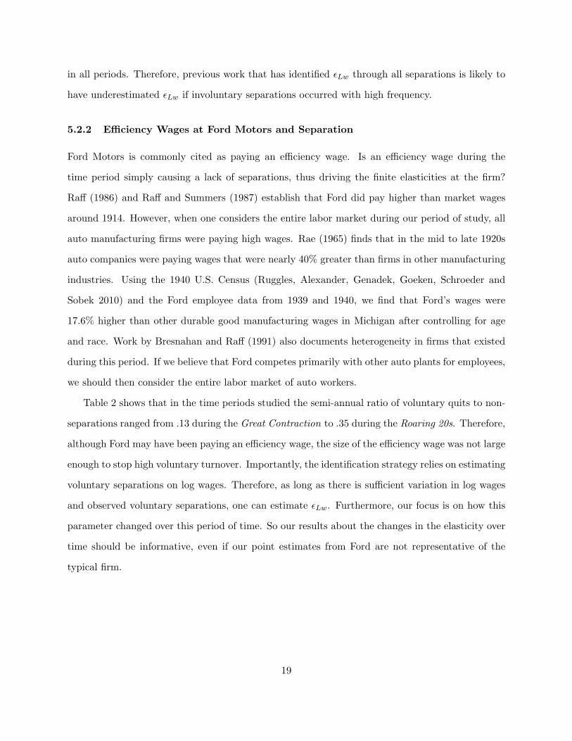
5.2.2 Efficiency Wages at Ford Motors and Separation
Ford Motors is commonly cited as paying an efficiency wage. Is an efficiency wage during the
time period simply causing a lack of separations, thus driving the finite elasticities at the firm?
Raff (1986) and Raff and Summers (1987) establish that Ford did pay higher than market wages
around 1914. However, when one considers the entire labor market during our period of study, all
auto manufacturing firms were paying high wages. Rae (1965) finds that in the mid to late 1920s
auto companies were paying wages that were nearly 40% greater than firms in other manufacturing
industries. Using the 1940 U.S. Census (Ruggles, Alexander, Genadek, Goeken, Schroeder and
Sobek 2010) and the Ford employee data from 1939 and 1940, we find that Ford’s wages were
17.6% higher than other durable good manufacturing wages in Michigan after controlling for age
and race. Work by Bresnahan and Raff (1991) also documents heterogeneity in firms that existed
during this period. If we believe that Ford competes primarily with other auto plants for employees,
we should then consider the entire labor market of auto workers.
Table 2 shows that in the time periods studied the semi-annual ratio of voluntary quits to non-
separations ranged from .13 during the Great Contraction to .35 during the Roaring 20s. Therefore,
although Ford may have been paying an efficiency wage, the size of the efficiency wage was not large
enough to stop high voluntary turnover. Importantly, the identification strategy relies on estimating
voluntary separations on log wages. Therefore, as long as there is sufficient variation in log wages
and observed voluntary separations, one can estimate εLw. Furthermore, our focus is on how this
parameter changed over this period of time. So our results about the changes in the elasticity over
time should be informative, even if our point estimates from Ford are not representative of the
typical firm.
19

5.3 Potential Wage Mark Downs and Pro-cyclical Real Wages
A firm facing a finite elasticity of supply is able to pay a wage less than the marginal revenue
product of labor. Therefore, given the pro-cyclicality of the labor elasticity of supply, the negative
effects of a recession can mitigated through lower labor costs. Table 8 reports the potential wage
markdown and its 95% confidence interval for the entire time period as well as the three major
sub-periods. We provide no evidence that Ford exploited the finite elastic labor supply and actually
paid workers less than their MRPL. The results suggest that during the Roaring 20s the potential
markdown on wages was 23% (wages potentially equated only 77% of MRPL). A perfectly inelastic
supply of labor to the firm during the Great Contraction suggests a potential 100% markdown of
wages. However, the upper-bound of the imprecise estimate suggests a potential markdown of only
27%. The expected New Deal period potential markdown was 18%.
The relationship between real wages and the business cycle has been studied in a number
of settings, including noncompetitive output markets and with price markups (Abraham and
Haltiwanger 1995). However, to our knowledge, the relationship has not been studied in a set-
ting with noncompetitive input markets, where firms can pay below the perfectly competitive wage
through finite εLw. A pro-cyclical εLw allows for firms to mark down wages during economic down-
turns and forces firms to pay more competitive wages during economic growth. Our results provide
an additional explanation for pro-cyclical real wages. Bils (1985) shows convincing evidence that
real wages are pro-cyclical by using disaggregated panel data. Beaudry and DiNardo (1991) de-
velops a contract model to understand how labor market conditions affect real wages. Under the
condition that mobility between firms is costly (labor market frictions), the model predicts the
unemployment rate at the time of hire and the individual’s entered into contract wage to be neg-
atively correlated. This is consistent with the monopsonistic outcome that labor market frictions
can grant firms the ability to pay workers less than their marginal revenue product of labor.
Solon, Whately and Stevens (1997) uses the Ford Motor Employee data set to try to explain that
empirical evidence suggests that real wages are pro-cyclical. While we focus on εLw as a potential
cause, they show that intra-firm mobility can also explain the pro-cyclicality of real wages for
individuals who do not separate from the firm.
20

6 Conclusion
Our study has for the first time addressed both theoretical and empirical evidence that the labor
elasticity of supply to the firm is pro-cylical. Comparative statics on the Burdett-Mortensen search
model predict that the labor elasticity of supply to the firm should increase during economic
expansion and decrease during economic contraction. Examining data that allows us to identify
the relationship between the elasticity and the business cycle, we find evidence that the elasticity is
lower during recessions than it is during expansions. Regressions that weight by the length of the
business cycles examined in our data allow us to reject the null hypothesis at the 5% level that the
mean elasticity is the same during expansionary and contractionary periods. Non-parametric tests
unequivocally allow us to reject a null that elasticities in these two states of the economy come
from the same data generating process.
We also present two identification related contributions. First, we derive a generalized estima-
tion strategy that can be applied to data sets where the firm’s employment level is not constant.
Second, we find that the inclusion of involuntary separations in the estimation of the elasticity of
supply to the fir can create significant attenuation bias if there is a high frequency of involuntary
quits.
The elasticity of supply to the firm potentially plays a large role in how wages and employ-
ment levels are determined within labor markets. A pro-cyclical labor elasticity of supply to the
firm allows firms to mark down wages during economic contractions and forces firms to pay more
competitive wages during economic expansions. This is consistent with recent work establishing
that wages are pro-cyclical, but under the scope of a new mechanism. It also provides insight into
how reduced labor costs for a firm can mitigate potential economic losses during a recession. Our
research adds to a small but growing literature on the elasticity and furthers future work with its
methodological contributions.
21

Table 1: Summary Statistics
Mean SD Min Max N1919(I)-1940(II)Separations 0.222 0.416 0.000 1.000 6979Wage 0.799 0.143 0.130 2.030 6979Age 31.201 7.413 15.000 57.500 6967Tenure 2.413 2.935 0.000 21.000 6967Married 0.535 0.499 0.000 1.000 6967Black 0.077 0.266 0.000 1.000 69671919(I)-1929(I)Separations 0.257 0.437 0.000 1.000 5255Wage 0.788 0.139 0.300 2.030 5255Age 30.567 6.644 16.500 57.500 5243Tenure 1.802 2.043 0.000 14.000 5243Married 0.527 0.499 0.000 1.000 5243Black 0.072 0.258 0.000 1.000 52431929(II)-1933(I)Separations 0.113 0.317 0.000 1.000 820Wage 0.878 0.169 0.130 1.630 820Age 34.659 7.955 18.000 51.000 820Tenure 4.273 3.438 0.000 14.500 820Married 0.632 0.483 0.000 1.000 820Black 0.066 0.248 0.000 1.000 8201933(II)-1940(II)Separations 0.123 0.328 0.000 1.000 904Wage 0.797 0.119 0.250 1.150 904Age 31.744 9.838 15.000 57.500 904Tenure 4.268 4.769 0.000 21.000 904Married 0.494 0.500 0.000 1.000 904Black 0.115 0.319 0.000 1.000 904
22

Table 2: Separations and Wage Changes at Ford
1919(I)-1940(II) 1919(I)-1929(I) 1929(II)-1933(I) 1933(II)-1940(II)# Stays 5422 3902 727 793# Quits 1545 1341 93 111# Fires 193 163 20 10# Layoffs 260 32 148 80Wage ∆ Per Worker 1.34 1.13 1.28 1.87∆ Up 0.89 0.92 0.65 0.93∆ Down 0.11 0.08 0.35 0.07Avg Days between ∆ 152.41 150.65 169.89 174.97
23

Tab
le3:
LP
ME
stim
ates
for
Yea
rs19
19(I
)th
roug
h19
40(I
I)
Yea
rF
Es
Yea
rF
Es
Yea
ran
dP
lant
FE
sY
ear
Pla
nt
and
Job
FE
sL
ogW
age
-0.4
7-0
.37
-0.3
9-0
.39
(0.0
39)
(0.0
40)
(0.0
41)
(0.0
42)
Bla
ck-0
.07
-0.0
7-0
.08
(0.0
16)
(0.0
16)
(0.0
17)
Age
0.01
0.01
0.01
(0.0
05)
(0.0
05)
(0.0
05)
Age
-Squ
ared
-0.0
0-0
.00
-0.0
0(0
.000
)(0
.000
)(0
.000
)T
enur
e-0
.04
-0.0
4-0
.03
(0.0
04)
(0.0
04)
(0.0
04)
Ten
ure-
Squa
red
0.00
0.00
0.00
(0.0
00)
(0.0
00)
(0.0
00)
Mar
ried
0.01
0.01
0.02
(0.0
11)
(0.0
11)
(0.0
11)
R-s
quar
ed0.
099
0.11
40.
117
0.12
3N
6979
6967
6967
6967
1R
obust
Sta
ndard
Err
ors
inpare
nth
eses
.
24

Table 4: Elasticity Estimates Over Major Sub-Periods
Spec 1 Spec 2 Spec 3 Spec 41919(I)-1940(II) 3.88 3.03 3.23 3.19
(0.31) (0.34) (0.33) (0.35)1919(I)-1929(I) 4.15 3.20 3.41 3.36
(0.30) (0.32) (0.32) (0.34)1929(II)-1933(I) 1.04 -1.29 -0.61 -0.90
(1.43) (1.65) (1.73) (1.84)1933(II)-1940(II) 4.54 4.30 4.63 4.70
(1.37) (1.39) (1.69) (1.70)1 Bootstrap standard errors presented in parentheses from 500
replications.
Table 5: Business Cycle (NBER) Estimates
Start Year End Year BS Direction Elasticity of Supply Markdown Obs1919(I) 1919(II) ↗ 1.59 0.39 228
(2.05)1920(I) 1921(I) ↘ 5.00 0.17 410
(1.18)1921(II) 1923(I) ↗ 3.82 0.21 977
(0.68)1923(II) 1924(I) ↘ 2.98 0.25 711
(0.89)1924(II) 1926(II) ↗ 3.90 0.20 1692
(0.81)1927(I) 1927(II) ↘ 0.72 0.58 363
(2.69)1928(I) 1929(I) ↗ 3.28 0.23 862
(0.82)1929(II) 1933(I) ↘ -0.90 1.00 820
(1.85)1933(II) 1937(I) ↗ 5.49 0.15 504
(2.10)1937(II) 1938(I) ↘ 3.49 0.22 118
(8.86)1938(II) 1940(II) ↗ 4.61 0.18 282
(2.95)a Bootstrap standard errors displayed in parentheses from 500 replications.
25
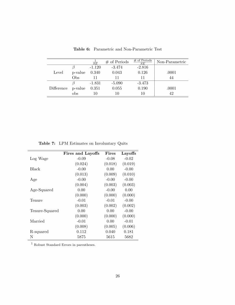
Table 6: Parametric and Non-Parametric Test
1SE # of Periods # of Periods
SE Non-Parametricβ -1.120 -3.474 -2.816
Level p-value 0.340 0.043 0.126 .0001Obs 11 11 11 44β -1.831 -5.090 -3.473
Difference p-value 0.351 0.055 0.190 .0001obs 10 10 10 42
Table 7: LPM Estimates on Involuntary Quits
Fires and Layoffs Fires LayoffsLog Wage -0.09 -0.08 -0.02
(0.024) (0.018) (0.019)Black -0.00 0.00 -0.00
(0.013) (0.009) (0.010)Age -0.00 -0.00 -0.00
(0.004) (0.003) (0.003)Age-Squared 0.00 -0.00 0.00
(0.000) (0.000) (0.000)Tenure -0.01 -0.01 -0.00
(0.003) (0.002) (0.002)Tenure-Squared 0.00 0.00 -0.00
(0.000) (0.000) (0.000)Married -0.01 0.00 -0.01
(0.008) (0.005) (0.006)R-squared 0.112 0.040 0.181N 5875 5615 56821 Robust Standard Errors in parentheses.
26

Tab
le8:
Bia
sR
educ
tion
and
Pot
enti
alW
age
Mar
kdow
na
Invo
lQ
uits
Una
djus
ted
Pre
ferr
edC
IC
IM
arkd
own
Mar
kdow
nM
arkd
own
Low
Hig
hH
igh
Low
1919
(I)-
1940
(II)
2.61
3.50
3.19
2.50
3.83
0.24
0.29
0.20
(0.3
0)(0
.39)
(0.3
5)19
19(I
)-19
29(I
)3.
163.
933.
362.
694.
030.
230.
270.
20(0
.31)
(0.4
0)(0
.34)
1929
(II)
-193
3(I)
-1.7
2-0
.59
-0.9
0-4
.51
2.72
1.00
1.00
0.27
(0.9
0)(1
.22)
(1.8
4)19
33(I
I)-1
940(
II)
3.65
5.53
4.70
1.37
8.03
0.18
0.42
0.11
(0.9
5)(2
.00)
(1.7
0)a
“M
ark
dow
n”
repre
sents
the
pote
nti
al
pro
port
ion
ofMRPL
that
wages
are
mark
eddow
n((MRPL−w
)/MRPL
)th
rough
the
firm
explo
itin
ga
finit
ela
bor
elast
icit
yof
supply
.
27
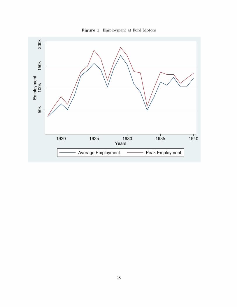
Figure 1: Employment at Ford Motors
50k
100k
150k
200k
Em
plo
ym
ent
1920 1925 1930 1935 1940Years
Average Employment Peak Employment
28

Figure 2: Elasticities over Time at Ford (1.5 Year Avg)
020
ur
01
510
Labor
Ela
sticity o
f S
upply
19 21 23 25 27 29 31 33 35 37 39Mid−Point Year
Estimated Elasticity Unemployment Rate
29

Figure 3: Elasticity of Supply to the Firm and the Business Cycle (NBER)
−2
02
46
Labor
Ela
sticity o
f S
upply
20 25 30 35 40Peaks and Troughs
Elasticity (Expansion) Elasticity (Contraction)
30

Figure 4: Separation Rates by Type
0.2
.4.6
Separa
tion R
ate
20 25 30 35 40Year
Voluntary Separations Involuntary Separations
31

References
Abraham, Katharine G. and John C. Haltiwanger, “Real Wages and the Business Cycle,”Journal of Economic Literature, 1995, 33 (3), 1215–1264.
Archives, Ford Motor Company, “Ford Motor Company Employment Statistics,” 1903-1972.
Beaudry, Paul and Jon DiNardo, “The Effect of Implicit Contracts on the Movement of WagesOver the Business Cycle: Evidence from Micro Data,” The Journal of Political Economy, 1991,99 (4), 665–688.
Bils, Mark J., “Real Wages over the Business Cycle: Evidence from Panel Data,” The Journalof Political Economy, 1985, 93 (4), 666–689.
Boal, William M., “Testing for Monopsony n Turn-of-the-Century Coal Mining,” The RANDJournal of Economics, 1995, 26 (3), 519–536.
and Michael R. Ransom, “Monopsony and the Labor Market,” Journal of EconomicLiterature, 1997, 35, 86–112.
Bresnahan, Timothy F. and Daniel M. G. Raff, “Intra-Industry Heterogeneity and the GreatDepression: The American Motor Vehicles Industry, 1929-1935,” The Journal of EconomicHistory, 1991, 51 (2), 317–331.
Burdett, Kenneth and Dale T. Mortensen, “Wage Differentials, Employer Size, and Unem-ployment,” Intenational Economic Review, 1998, 39 (3), 257–273.
Card, David E. and Alan B. Krueger, Myth and Measurement: The New Economics of theMinimum Wage, Princeton, NJ: Princeton University Press, 1995.
Coen, Robert M., “Labor Force and Unemployment in the 1920’s and 1930’s: A Re-ExaminationBased on Postwar Experience,” The Review of Economics and Statistics, 1973, 55 (1), 46–55.
Committee, NBER’s Business Cycle Dating, Business Cycle Definitions, Cambridge, MA:National Bureau of Economic Research, Inc., 2011.
Dube, Arindrajit, T. William Lester, and Michael Reich, “Do Frictions Matter in theLabor Market? Accessions, Separations and Minimum Wage Effects,” IZA Discussion PaperSeries, 2011, 5811.
Falch, Torberg, “The elasticity of labor supply at the establishment level,” Journal of LaborEconomics, 2010, 28 (2).
, “Teacher Mobility Responses to Wage Changes: evidence from a quasi-natural experiment,”American Economic Review, 2011, 101 (2).
Fishback, Price V., “New Deal,” in Steven N. Durlauf and Lawrence E. Blume, eds., The NewPalgrave Dictionary of Economics, Basingstoke: Palgrave Macmillan, 2008.
Foote, Christopher L., Warren C. Whatley, and Gavin Wright, “Arbitraging a Discrim-inatory Labor Market: Black Workers at the Ford Motor Company, 1918-1947,” Journal ofLabor Economics, 2003, 21 (3), 493–532.
32

Hirsch, Boris, “Joan Robinson Meets Harold Hotelling: A Dyopsonistic Explanation of the GenderPay Gap,” BGPE Discussion Papers 24, Bavarian Graduate Program in Economics (BGPE)Jun 2007.
, Thorsten Shank, and Claus Schnabel, “Gender Differences in Labor Supply to Monop-sonistic Firms: An Empirical Analysis Using Linked Employer-Employee Data from Germany,”IZA Discussion Papers 2443, Institute for the Study of Labor (IZA) Nov 2006.
, , and , “Differences in Labor Supply to Monopsonistic Firms and the Gender PayGap: An Empirical Analysis Using Linked Employer-Employee Data from Germany,” Journalof Labor Economics, 2010, 28 (2), 291–330.
Hotchkiss, Julie L. and Myriam Quispe-Agnoli, “Employer Monopsony Power in the LaborMarket for Undocumented Workers,” Federal Reserve Bank of Atlanta Working Paper, 2009,14a.
Maloney, Thomas and Warren Whatley, “Making the Effort: The Racial Contours of Detroit’sLabor Market, 1920-1940,” Journal of Economic History, 1995, 55, 465–93.
Manning, Alan, Monopsony in Motion: Imperfect Competition in Labor Markets, Priceton, N.J.:Princeton University Press, 2003.
Rae, J. B., The American Automobile: A Brief History, Chicago, IL: The University of ChicagoPress, 1965.
Raff, D. M. G., “Wage Determination Theory and the Five Dollar Day at Ford,” The Journal ofEconomic History, 1986, 48 (2), 387–399.
Raff, Daniel M. G. and Lawrence H. Summers, “Did Henry Ford Pay Efficiency Wages?,”Journal of Labor Economics, 1987, 5 (4).
Ransom, Michael R., “Seniority and Monopsony in the Academic Labor Market,” AmericanEconomic Review, 1993, 83 (1), 221–233.
and David P. Sims, “Estimating the Firm’s Labor Supply Curve in a “New Monopsony”Framework: School Teachers in Missouri,” IZA Discussion Papers 4271, Institute for the Studyof Labor (IZA) Jun 2009.
and Ronald L. Oaxaca, “Sex Differences in Pay in a ”New Monopsony” Model of the LaborMarket,” IZA Working Paper, 2005, 1870.
and , “New Market Power Models and Sex Differences in Pay,” Journal of Labor Eco-nomics, 2010, 28 (2), 267–290.
and Val E. Lambson, “Monopsony, Mobility, and Sex Differences in Pay: Missouri SchoolTeachers,” American Economic Review, 2011, 101 (3), 454–59.
Robinson, Joan, The Economics of Imperfect Competition, London, UK: Macmillan and Co. ltd.,1933.
33
Romer, Christina, “Spurious Volatility in Historical Unemployment Data,” The Journal of Po-litical Economy, 1986, 94 (1), 1–37.
Ruggles, Steven, J. Trent Alexander, Katie Genadek, Ronald Goeken, Matthew B.Schroeder, and Matthew Sobek, Integrated Public Use Microdata Series: Version 5.0[Machine-readable database] 2010.
Solon, Gary, Warren Whately, and Ann Huff Stevens, “Wage Changes and Intrafirm JobMobility over the Business Cycle: Two Case Studies,” Industrial and Labor Relations Review,1997, 50 (3), 402–415.
Staiger, Douglas O., Joanne Spetz, and Ciaran S. Phibbs, “Is There Monopsony in theLabor Market? Evidence from a Natural Experiment,” Journal of Labor Economics, 2010, 28(2), 211–236.
Whatley, Warren C. and Gavin Wright, Employee Recoreds of the Ford Motor Company[Detroit Area], 1918-1947, Ann Arbor, Michigan: Inter-university Consortium for Politicaland Social Research, 1995.
and Stan Sedo, “Quit Behavior as a Measure of Worker Opportunity: Black Workers in theInterwar Industrial North,” The American Economic Review Papers and Proceedings, 1998,88 (2), 363–367.
34
A Appendix
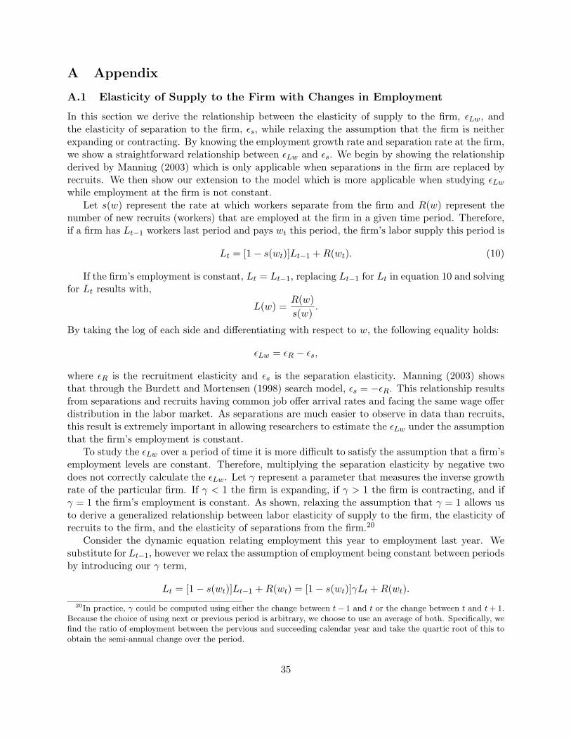
A.1 Elasticity of Supply to the Firm with Changes in Employment
In this section we derive the relationship between the elasticity of supply to the firm, εLw, andthe elasticity of separation to the firm, εs, while relaxing the assumption that the firm is neitherexpanding or contracting. By knowing the employment growth rate and separation rate at the firm,we show a straightforward relationship between εLw and εs. We begin by showing the relationshipderived by Manning (2003) which is only applicable when separations in the firm are replaced byrecruits. We then show our extension to the model which is more applicable when studying εLwwhile employment at the firm is not constant.
Let s(w) represent the rate at which workers separate from the firm and R(w) represent thenumber of new recruits (workers) that are employed at the firm in a given time period. Therefore,if a firm has Lt−1 workers last period and pays wt this period, the firm’s labor supply this period is
Lt = [1− s(wt)]Lt−1 +R(wt). (10)
If the firm’s employment is constant, Lt = Lt−1, replacing Lt−1 for Lt in equation 10 and solvingfor Lt results with,
L(w) =R(w)s(w)
.
By taking the log of each side and differentiating with respect to w, the following equality holds:
εLw = εR − εs,
where εR is the recruitment elasticity and εs is the separation elasticity. Manning (2003) showsthat through the Burdett and Mortensen (1998) search model, εs = −εR. This relationship resultsfrom separations and recruits having common job offer arrival rates and facing the same wage offerdistribution in the labor market. As separations are much easier to observe in data than recruits,this result is extremely important in allowing researchers to estimate the εLw under the assumptionthat the firm’s employment is constant.
To study the εLw over a period of time it is more difficult to satisfy the assumption that a firm’semployment levels are constant. Therefore, multiplying the separation elasticity by negative twodoes not correctly calculate the εLw. Let γ represent a parameter that measures the inverse growthrate of the particular firm. If γ < 1 the firm is expanding, if γ > 1 the firm is contracting, and ifγ = 1 the firm’s employment is constant. As shown, relaxing the assumption that γ = 1 allows usto derive a generalized relationship between labor elasticity of supply to the firm, the elasticity ofrecruits to the firm, and the elasticity of separations from the firm.20
Consider the dynamic equation relating employment this year to employment last year. Wesubstitute for Lt−1, however we relax the assumption of employment being constant between periodsby introducing our γ term,
Lt = [1− s(wt)]Lt−1 +R(wt) = [1− s(wt)]γLt +R(wt).20In practice, γ could be computed using either the change between t− 1 and t or the change between t and t+ 1.
Because the choice of using next or previous period is arbitrary, we choose to use an average of both. Specifically, wefind the ratio of employment between the pervious and succeeding calendar year and take the quartic root of this toobtain the semi-annual change over the period.
35

Therefore,
Lt =R(wt)
1− [1− s(wt)]γ. (11)
Taking logs and simplifying, we have
ln(Lt) = ln(R(wt))− ln(1 + s(wt)γ − γ).
Differentiating the above equation and multiplying by w we have
εLw = εR −γs′(wt)wt
1 + γs(wt)− γ
εLw = εR − εss(wt)γ
1 + γs(wt)− γ(12)
We can see above that there is now a more complex relationship between changes in wages andchanges in labor supply to the firm. We have found the effect through separations.
Our challenge now is to find εR in terms of εs. To do this, we turn to the definition of therecruitment elasticity and then to the search model. The elasticity of recruitment with respect tothe wage can be expressed by
εR =w ×R′(w)R(w)
. (13)
Under the Burdett and Mortensen (1998) model, the recruitment function is given by
R(w) = Ru + λ
∫ w
0f(x)L(x)dx,
where Ru is the amount of recruits that are hired from unemployment, λ is the job offer arrivalrate, f(w) is the density wage offers. Thus,
R′(w) = λf(w)L(w). (14)
Therefore, using equation (14) and (13), we have
εR =wλf(w)L(w)
R(w). (15)
By combining equation (11) and (15) the elasticity or recruitment with respect to wage is,
εR =wλf(w)
1 + s(w)γ − γ(16)
Last, we must consider the separations side of the Burdett and Mortensen model in order tofind the relationship between εR and εs. Separations in this model are given by
s(w) = δ + λ[1− F (w)],
where δ is the exogenous job destruction rate, λ is the job offer arrival rate and F (w) the distributionof wage offers. The derivative of the separation function with respect to the wage is then
s′(w) = −λf(w). (17)
36

Therefore by combining equation (16) and (17) the elasticity of recruitment is
εR =−ws′(w)
1− (1− s(w))γ,
εR = −εss(w)
1− (1− s(w))γ. (18)
Finally, by substituting equation (18) into equation (12), the elasticity of labor supply withrespect to wage can be identified through the separation elasticity of wage, εs, the separation rate,s(w), and rate of expansion or contraction of the firm, γ. We find that
εLw = −(1 + γ)εss(w)
1− (1− s(w))γ.
This derived adjustment is consistent with Manning (2003) as the equation collapses to εLw =−2εs when employment is constant over time (γ = 1). Note that the lower bound on s(w) isdetermined by γ. As R(w) ≥ 0, then s(w) ≥ 1− 1
γ .
37

A.2 Appendix Tables and Figures
38

Tab
le1:
LP
ME
stim
ates
for
Maj
orSu
b-P
erio
ds
1919
(I)-
1940
(II)
1919
(I)-
1929
(I)
1929
(II)
-193
3(I)
1933
(II)
-194
0(II
)L
ogW
age
-0.3
9-0
.50
0.03
-0.3
4(0
.042
)(0
.050
)(0
.066
)(0
.116
)B
lack
-0.0
8-0
.07
0.05
-0.1
1(0
.017
)(0
.021
)(0
.062
)(0
.031
)A
ge0.
010.
02-0
.02
0.02
(0.0
05)
(0.0
08)
(0.0
13)
(0.0
10)
Age
-Squ
ared
-0.0
0-0
.00
0.00
-0.0
0(0
.000
)(0
.000
)(0
.000
)(0
.000
)T
enur
e-0
.03
-0.0
5-0
.00
-0.0
1(0
.004
)(0
.007
)(0
.011
)(0
.008
)T
enur
e-Sq
uare
d0.
000.
00-0
.00
0.00
(0.0
00)
(0.0
01)
(0.0
01)
(0.0
00)
Mar
ried
0.02
0.02
0.00
0.03
(0.0
11)
(0.0
13)
(0.0
28)
(0.0
34)
R-s
quar
edN
7070
5346
820
904
1R
obust
Sta
ndard
Err
ors
inpare
nth
eses
.
39
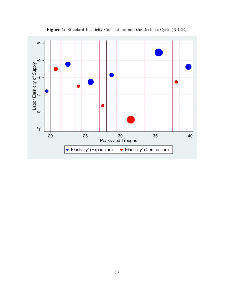
Figure 1: Standard Elasticity Calculations and the Business Cycle (NBER)
−2
02
46
8Labor
Ela
sticity o
f S
upply
20 25 30 35 40Peaks and Troughs
Elasticity’ (Expansion) Elasticity’ (Contraction)
40