ELASTIC LAYER ANALYSIS RELATED TO PERFORMANCE IN FLEXIBLE PAVEMENT DESIGN Friedrich W. Jung and William A. Phang,

:Ministry of Transportation and Communications, Ontario

From experience in Ontario with flexible pavements and from results of the AASHO Road Test, it was found that the calculated subgrade deflection under a standard wheel load is the best indicator of performance of the pavement as a whole when it is compared with other stress, strain, and deformation values calculated by elastic layer theory. In the calculations, layer equivalencies obtained from experience and variations in subgrades were expressed in terms of elastic moduli. Subgrade deflections can be calculated more simply by using Odemark's concept of equivalent layer thickness. Expressions for load equivalency factors were derived from AASHO Road Test data by using this simplified deflection calculation. Finally, a functional relationship between subgrade deflection, number of standard load applications, and present serviceability index was estab­lished. The findings constitute major parts of a design subsystem to be used within a management system for flexible pavements.

•THROUGH a process of continual pavement evaluation, pavement design engineers in Ontario were able to compile a table of successful thickness designs (1). The table recognizes differences in thickness caused by the traffic, road class, and type of subgrade. Elastic layer analysis was used to examine the table to find a more rational method of flexible pavement design. It was hoped that a possible clue to the success of the conventional designs listed in the table might be found.

The method of investigation was to assign values of elastic moduli to each pavement layer and subgrade class and to calculate stresses, strains, and deflections in each layer for a standard wheel load. The elastic moduli assigned to each pavement layer and to each class of subsoil were selected after a study of available literature. The calculated stresses, strains, and deflections were examined for a constant value of these parameters within each traffic or highway class. A constant value within the same road class over the six major subgrade types identified within Ontario could in­dicate a common distress mechanism and would provide a practical criterion for design.

In this process of calculation, in which the Chevron computer program was used, many different sets of moduli were assigned to the pavement layers and subgrades. Through this procedure, it was discovered that only the vertical deflection on top of the subgrade emerged as the response value, which could be made to remain constant within each traffic or road class. Several sets of assumed moduli were successful in this respect. Subgrade deflections were also calculated by a simplified method that uses the principle of equivalent layer thickness as proposed by Odemark (3).

The course of investigation was then directed to the best documented experiment available.

AASHO ROAD- TEST

Two sets of moduli, which had been applied successfully to the Ontario designs,

Publication of this paper sponsored by Committee on Flexible Pavement Design.

14

15

were assigned to the layers of the main factorial designs of the AASHO Road Test (5, 6), and the subgrade deflections were calculated for both the applied single-axle load in- -each loop and the standai·d 18-kip (80 kN) axle load. A statistical analysis of these cal­culated deflections not only resulted in a formula for load equivalency factors but cul­minated in finding a relationship between the loss of performance or serviceability and the number of equivalent standard load applications for given values of subgrade de­flection.

By using sets of elastic moduli for calculating subgrade deflections, we demonstrated that this deflection is linked to standards of performance or serviceability. The design subsystem of this research is shown in Figure 1. An equation was derived for deter­mining the necessary total equivalent granular thickness so that the design method could be completed.

EXPLORING SUCCESSFUL ONTARIO DESIGNS

Ontario's successful designs, which have survived an average of about 11.5 years , are given in Tables 1 and 2. The lines in the table pertain to traffic or road classes indicated by approximate average daily traffic values. The columns of the table pertain to the types of subgrade soils as they are classified in Ontario.

For each of the calculations, basically two sets of moduli were assumed and sub­sequently varied and modified into different sets with which calculations were continued. These two sets wer e the subgrade moduli E. , which constitute a decreasing sequence from hard subgrades (gra nular) to soft subgrades (soft clay) and the layer moduli E1,

E2, and E3 for asphaltic hot mix, granular base, and sand subbase. Cases 1, 2, 3, and 4 of these calculations were finally assembled, which may be thought of as being based on true or realistic relations between the assumed moduli. The moduli E1 , E2, and E3 of these four cases are related to the layer equivalencies, valid in Ontario, as follows:

hot mix : base : subbase = 1 : 2 : 3 = _l_ : _l_ : _l_ Wi .:IEz ~

(1)

The relationship between the set of layer moduli and the set of subgrade moduli is dif­ferent in all four cases, and this indicates insensitivity about this relationshiJ?.

For a wheel load of 9,000 lb (40 kN) and a pres sure area r adius of 6.4 in. (16.3 cm), all stresses, strains, and deflections at the layer interfaces were calculated. The most important of these are shown in Figure 2 and their values for cases 3 and 4 are given in Tables 3 and 4. In all four cases assembled, only the deflections on top of the subgrade were approximately equal for each of the five traffic or road classes. This indicates that this deflection could be a powerful design criterion.

SUBGRADE DEFLECTION AS DESIGN CRITERION

The calculations on the successful Ontario designs revealed that the most promising design parameter for flexible pavements was the vertical deflection on top of the sub­grade. This hypothesis is in line with previous research find ings (2) in which the ver­tical compressive strain on the subgrade was declared the dominating design parameter. These findings were based on the AASHO Road Test, which was carried out on the same subsoil. For constant subgrade modulus the two criteria are indeed equivalent, but the strain criterion obviously breaks down if a wide range of subgrades is considered. The same is true for the corresponding stress.

Tensile stress or strain in the asphaltic layer must be considered, although it is probably a secondary design criterion. For instance, the thickness of the asphaltic layer s , as a portion of the total equivalent thickness, could possibly be determined by the magnitude of tensile strain under r epeated loads (fatigue) and under var ying tem­perature conditions, whereas the total thickness is still determined by the subgrade deflection.

If only subgrade deflections are needed, the-11 it is more economical to calculate them by t he method suggested py Odemark (~,_±). The deviations of the following de­sign equations based on subgrade deflections can be studied in more detail in the

Figure 1. Pavement design subsystem.

Structural

h1, h,, h,

Material

E 1 , E,, E,, Em

Load

P a

Environment

Construction

etc

Model of the Pavement

Structure: E li,stic Layer

System

EXPERIMENT and EXPERIENCE

AASHO Road Test data

Ontario's successful des.

RESPONSE

Subgrade Deflection w

as Distress

Indicator

Brampton Road Test data 1------~ BBR

.--B-e-n-ke_l_m_a_n_B_e_a_m_d_a_t_a_S ___ "'i-- ---+18~

Table 1. Moduli of successful Ontario designs.

Subgrade Material, psi

Grain Type Sandy Silt and Clay, Loam Till of Materials Suitable as Silt <40, Very Silt 40 to 50, Silt >50, Very Granular Fine Sand Very Fine Sand Fine Sand

Case Modulus Borrow and Silt <45 and Silt 45 to 60 and Silt >60

E, 400,000 400, 000 400,000 400,000 E, 50,000 50,000 50,000 50,000 E, 15,000 15,000 15,000 E,, 15,000 8, 500 7,000 5,700

2 E, 320,000 320,000 320,000 320, 000 E, 40,000 40,000 40,000 40,000 E, 12,000 12,000 12,000 E, 15,000 8,400 6,900 5,700

E, 400,000 400,000 400,000 400,000 E, 50,000 50,000 50,000 50,000 E, 15,000 15,000 15,000 E, 11,000 6,000 5,000 4,000

4 E, eoo;ooo 600,000 600,000 600,000 E, 75,000 75,000 75,000 75,000 E, 22, 000 22,000 22,000 E, 11,000 6,000 5,000 4,000

Note: 1 psi • 6.8948 kPa,

OUTPUT FUNCTION

Deterioration

Applications N

Clay

Solt Hard Varved Lacuetrine and Leda

400,000 400,000 50,000 50,000 15,000 15,000

7,500 3,800

320,000 320 000 40,000 40, 000 12,000 12,000

7,600 3,900

400,000 400,000 50,000 50,000 15,000 15,000

5,300 2,700

600,000 600,000 75,000 75,000 22,000 22,000

5,300 2,700

Table 2. Average subgrade deflections of successful Ontario designs.

Subgrade Material Thickness, in.

Grain Type Sandy Silt and Clay Loam Till of Mate- Clay rials Suit- Silt <40, Silt 40 to 50, Silt .>50, able as Very Fine Very Fine Very Fine Soft

Thick- Granular Sand and Sand and Sand and Hard Varved Class and Road ness Borrow Silt <45 Silt 45 to 60 Silt >60 Lacustrine and Leda Average Deflection Values, in. b

King's highways Multilane h, 5.5 5.5 5.5 5.5 5.5 5.5 0.0128 0.0136 0.0163 0.0144

h, 7.5, 6.5' 6 6 6 6 6 h, 15 21,201 27 18 42 0.0119 0.0129 0.0152 0.0133

Two lanes, h, 4.5 4.5 4.5 4.5 4.5 4.5 0.0136 0.0145 0.0172 0.0151 AADT h, 7.5 6 6 6 6 6 >2,000 II, 15 21, 20' 27 18 42 0.0128 0.0138 0.0162 0.0142

Two lanes, h, 3.5 3.5 3.5 3.5 3.5 3.5 0.0167 0.0178 0.0212 0.0186 AADT h, 6 6 6 6 6 6 <2,000 h, 12, 11' 15 21 12 30 0.0159 0.0170 0.0206 0.0177

3econdary roads, h, 1.5 r{· 5 1.5 1.5 1.5 1.5 0.0202 0.0217 0.0259 0.0227 AADT >1,000 h, 6, 6 . 5' 6 6 6 6

h, 9 12 21, 18' 12 30, 27' 0.0200 0.0200 0.0260 0.0230

rownship roads, h, 1.5 1. 5 1.5 1.5 1.5 1.5 0.0268 0.0286 0.0347 0.0297 AADT >200 h, 4 6 6 6 6 6

h, 4 6 9 6 18 0.0260 0.0280 0.0338 0.0298

Note: 1 in. ::a 2.54 cm.

•Modified thicknesses only used for cases 3 and 4, bUpper values for each entry set are for Chevron; the bottom for Odemark ,

Table 3. Calculated criteria for case 3.

Subgrade Material

Grain Type Sandy Silt and Clay Loam Till of Mate-rials Suit- Silt <40, Silt 40 to 50, Silt >50, Average able as Very Fine Very Fine Very Fine Clay Deflection

Type of Criterion or Distress Granular Sand and Sand and Sand and Values Class of Road Indicator Borrow• Silt <45' Silt >45° Slit >60' Hard' Soft1 (in.)

King's highways Multilane Subgrade deflection, Chevron, in. 0.0157 0.0159 0.0163 0.0168 0.0162 0.0171 0.0163

Subgrade deflection, Odemark, in. 0.0152 0.0151 0.0158 0.0153 0.0153 0.0155 0.0152 Total deflection, Chevron, in. 0.0186 0.0236 0.0249 0.0265 0.0246 0.0284 0.0244 Total deflection, Odemark, in. 0.0168 0.0191 0.0194 0.0198 0.0194 0.0199 0.0191

Two lanes, SUbgrade deflection, Chevron, in. 0.0167 0.0170 0.0177 0.0176 0.0172 0.0179 0.0172 >2,000 AADT Subgrade deflection, O:lemark, in. 0.0161 0.0162 0.0172 0.0162 0.0164 0.0162 0.0162

Total deflection, Chevron, in. 0.0203 0.0262 0.0274 0.0289 0.0271 0.0308 0.0268 Total deflection, Odemark, in. 0.0182 0.0211 0.0213 0.0214 0.0213 0.0214 0.0208

Two lanes, Subgrade deflection, Chevron, 10. 0.0207 0.0208 0.0206 0.0207 0.0216 0.0228 0.0212 <2,000 AADT Subgrade deflection, Odemark, in. 0.0200 0.0199 0.0199 0.0198 0.0210 0.0211 0.0203

Total deflection, Chevron, in. 0.0245 0.0306 0.0319 0.0334 0.0321 0.0370 0.0316 Total deflection, Odemark, in. 0.0223 0.0251 0.0255 0.0256 0.0261 0.0267 0.0252

Secondary road, Subgrade deflection, Chevron, in. 0.0262 0.0263 0.0264 0.0250 0.0254 0.0263 0.0259 paved >1, 000 Subgrade deflection, Odemark, in. 0.0263 0.0266 0.0267 0.0253 0.0257 0.0257 0.0260 AADT Total deflection, Chevron, in. 0.0316 0.0402 0.0418 0.0426 0.0408 0.0460 0.0405

Total deflection, Odemark, in. 0.0305 0.0354 0.0360 0.0353 0.0352 0.0357 0.0346

Township road, Subgrade deflection, Chevron, in. 0.0334 0.0357 0.0340 0.0344 0.0327 0.0326 0.0347 paved >200 AADT Subgrade deflection, Odemark, in. 0.0334 0.0337 0.0346 0.0351 0.0332 0.0332 0.0338

Total deflection, Chevron, in. 0.0376 0.0487 0.0463 0.0488 0.0449 0.0505 0.0461 Total deflection, Odemark, in. 0.0362 0.0400 0.0415 0.0427 0.0403 0.0416 0.0404

King's highways Multllane Vertical subgrade stress, psi -6.88 -2.09 -1.51 -1.03 -1. 70 -0.532

Vertical subgrade strain, in. -0.000505 -0.000314 -0.000269 -0.000223 -0.000287 -0.000167 Radial asphalt stress, psi 142.0 142.0 140.0 139.0 141.0 137.0 Radial asphalt strain, in. 0.000204 0.000204 0.000202 0.000200 0.000203 0.000198

Two lanes, Vertical subgrade strain, psi -7.82 -2.44 -1.72 -1.14 -1.96 -5.69 >2,000 AADT Vertical subgrade strain, in. -0.000583 -0.000370 -0.000311 -0.000251 -0.000334 -0.000179

Radial asphalt stress, psi 153.0 159.0 157.0 156.0 158.0 154.0 Radial asphalt strain, in. 0.000227 0.000233 0.000231 0.000230 0.000232 0.000227

Two lanes, Vertical subgrade stress, psi -11.7 -3.72 -2.55 -1.64 -3.14 -8.98 <2,000 AADT Vertical subgrade strain, in. -0.000849 -0.000535 -0.000467 -0.000369 -0.000543 -0.000285

Radial asphalt stress, psi 179.0 173.0 171.0 169.0 172.0 167.0 Radial asphalt strain, in. 0.000269 0.000262 0.000260 0.000258 0.000262 0.000256

Secondary road, Vertical subgrade stress, psi -18.9 -6.03 -4.30 -2.51 -4.45 -1.22 paved >1, 000 Vertical subgrade strain, in. -0.000138 -0.000925 -0.000793 -0.000574 -0.000776 -0.000395 AADT Radial asphalt stress, psi 82.0 74.9 73.1 73.6 74.0 74.4

Radial asphalt strain, in. 0.000186 0.000176 0.000174 0.000175 0.000175 0.000176

Township road, Vertical subgrade stress, psi -28.3 -10.6 -6.99 -4.73 -7.24 -1.95 paved >200 Vertical subgrade strain, in. -0.001870 -0.001570 -0.001270 -0.001080 -0.001240 -0.000645 AADT Radial asphalt stress, psi 135.0 117.0 72.3 68.7 73.2 69.4

Radial asphalt strain, in. 0.000264 0.000223 0.000172 0.000168 0.000174 0.000170

Note: Modulus of (a) hot mix asphalt E 1 :::: 400,000; (b) the base E2 c 50,000; and (cl the subbase E3 = 15,000. 1 in~= 2.54 cm. 1 psi • 6~8948 kPa.

• Em • 11,000. bEm ""6,000~ "Em= 5,000~ dEm = 4,000 . eEm • 5,300, 'Em • 2,700.

Figure 2. Diagram of multilayer structure.

Table 4. Calculated criteria for case 4.

Type of Criterion or Distress Claes of Road Indicator

King 1s highways Multilane Subgrade deflection, Chevron, in.

Subgrade deflection, Odemark, in. Total deflection, Chevron, in. Total deflection, Odemark, in.

Two lanes, Subgrade deflection, Chevron, in. >2,000 AADT Subgrade deflection, Odemark, in.

Total deflection, Chevron, in. Total deflection, Odemark, in.

Two lanes, Subgrade deflection, Chevron, in. <2,000 AADT Subgrade deflection, Odemark, in.

Total deflection, Chevron, in~ Total deflection, Odemark, in.

Secondary road, Subgrade deflection, Chevron, in. paved >l,000 Subgrade deflection, Odemark, in. AADT Total deflection, Chevron, in,

Total deflection, Odernark, in.

Township road, Subgrade deflection, Chevron, in. paved >200 AADT Subgrade deflection, Odernark, in.

Total deflection, Chevron, in. Total deflection, Odemark, in.

King's highways Multilane Vertical subgrade stress, psi

Vertical subgrade strain, in. Radial asphalt stress, psi Radial asphalt strain, in.

Two lanes, Vertical subgrade stress, psi >2,000 AADT Vertical subgrade strain, in.

Radial asphalt stress, psi Radial asphalt strain, in.

Two lanes, Vertical subgrade stress, psi <2, 000 Vertical subgrade strain, in.

Radial asphalt stress, psi Radial asphalt strain, in.

Secondary road, Vertical subgrade stress, psi paved >1,000 Vertical subgrade strain, in. AADT Radial asphalt stress, psi

Radial asphalt strain, in.

Township road, Vertical subgrade stress, psi paved >200 AADT Vertical subgrade strain, in.

Radial asphalt stress, psi Radial asphalt strain, in.

CONTACT STRESS CT0

BITUMEN-B0Ui'O LAYERS ( MODULUS E 1 )

GRANULAR BASE AND SUIIBASE

/ TENSILE STRESS

----+----. OR STRAIN

(MODULUS E2 ,E 3 )

TOTAL DEFLECTION

h,

h2 +h,

SleGRADE "'CONfRESSIVE STRAIN, STRESS (MODULUS Em) OR DEFLECTION Of" SUIGRADE

Subgrade Material

Grain Type Sandy Silt and Clay Loam Till of Mate-rials Suit- Silt <40, Silt 40 to 50, Silt >50, able as Very Fine Very Fine Very Fine Clay Granular Sand and Sand and Sand and Borrow• Silt <45b Silt >45° Silt >60d Hard' Softr

0.0136 0.0141 0.0145 0.0150 0.0144 0.0146 0.0134 0.0132 0.0133 0.0134 0.0134 0.0136 0.0159 0.0195 0.0205 0.0217 0.0202 0.0225 0.0143 0.0154 0.0157 0.0159 0.0157 0.0161 0.0146 0.0150 0.0153 0.0157 0.0153 0.0152 0.0142 0.0143 0.0143 0.0142 0.0144 0.0142 0.0172 0.0214 0.0223 0.0235 0.0221 0.0243 0.0153 0.0170 0.0171 0.0172 0.0171 0.0172 0.0162 0.0181 0.0181 0.0164 0.0189 0.0201 0.0177 0.0175 0.0175 0.0174 0.0184 0.0165 0.0210 0.0250 0.0260 0.0271 0.0262 0.0299 0.0190 0 .0204 0.0206 0.0206 0.0213 0.0217

0.0231 0 .0230 0.0230 0.0220 0.0221 0.0233 0.0235 0.0235 0.0235 0.0223 0.0226 0.0226 0.0270 0.0327 0. 0337 0.0341 0.0326 0.0368 0.0261 0.0266 0.0289 0.0260 0.0261 0.0283

0.0249 0.0314 0.0297 0.0299 0.0286 0.0268 0.0302 0 .0298 0.0305 0.0309 0.0293 0,0290 0.0332 0.0406 0.0364 0.0400 0.0372 0.0411 0.0320 0.0335 0.0345 0.0353 0.0334 0.0339

-5.43 -1.64 -1.20 -0.624 -1.34 -0.426 -0.000368 -0.000242 -0 .000207 -0. 00172 -0.000220 -0.000130 151.0 144.0 142.0 140.0 143.0 137.0 0.000142 0.000137 0.000136 0.000134 0.000136 0.000132 -6.17 -1.91 -1.36 -0.910 -1.54 -0.455 -0.000447 -0.000286 -0.000238 -0.000193 -0.000257 -0.000139 161.0 161.0 158.0 156.0 159.0 153 .0 0.000157 0.000157 0.000155 0.000153 0.000156 0.000151 -9.29 -2. 92 -1.99 -1.29 -2.54 -0.715 -0.00656 -0.000412 -0.000356 -0.000260 -0.000419 -0.000217 190.0 175.0 172.0 169.0 174.0 167.0 0,000188 0.000176 0.000174 0.000172 0.000176 0.000170

-15,10 -4.75 -3, 36 -1.95 -3.49 -0 .966 -0.001070 -0.000722 -0.000611 -0. 000435 -0 .000600 -0.00296 80.6 69.1 67.9 69.6 66.7 71.1 0.000122 0.000112 0.000112 0.000113 0.000112 0.000114

-23.30 -8.44 -5.46 -3.67 -5.66 -1.51 -0.000490 -0.001240 -0.000984 -0.000622 -0 ,000965 -0.000480 150.0 114.0 66.2 62 .9 67.2 65.5 0.000173 0.000146 0.000110 0.000107 0.000110 0.000110

Note: Modulus of (a) the hot-mix asphalt E, = 600,000; (b) the base E2 = 75,000; and (c) the subbase E3 = 22,000. 1 in~= 2.54 cm. 1 psi= 6.8948 kPa.

a Em - 11,000, bEm = 6,000, cEm - 5,000. dEm ""4,000. eEm = 5,300. 1Em = 2,700.

Averag Deflect Values (m. )

0.0144 0.0134 0.0200 0.0155 0.0151 0.0143 0.0216 0.0166 0.0186 0.0176 0.0259 0.0206

0.0227 0.0230 0.0326 0.0260

0.0297 0.0299 0. 0364 0.0336

19

Appendix. The variable measurements may be either U.S. customary or metric units.

where

and where

p 1 W=--X---

2E.z Ca vi + ;:; z

m-1

z = 0.9 X L h1

i=l

w = subgrade deflection in inches; m = number of layers including subgrade; h1 = thickness of layer i in inches; E1 = modulus of layer i in psi; E. = subgrade modulus in psi; a = radius of loaded area in inches; and P = wheel load in lb.

(2)

(3)

The deflections w calculated in Eqs. 1 and 2 differ slightly from the subgrade de­flections calculated with the Chevron program (Tables 2, 3, and 4). The correlation coefficient r between the two calculated deflections, however, was found to be close enough to unity (r = 0.993 to 0,997) so that the much simpler method of calculation by Eqs. 2 and 3 is justified. The correlation between the two deflections of case 3 is shown in Figure 3.

SUBGRADE DEFLECTIONS OF AASHO ROAD TEST SECTIONS

Subgrade deflections w have been calculated for all designs given in Tables 1 and 2 and, for the moduli of cases 1 through 4, these deflections were approximately equal for each highway traffic class. In these calculations the applied load was constant, but the subgrade material E. was one of the main variables.

In contrast to this, the main factorial design sections of the AASHO Road Test were built on a uniform subgrade material (soft clay), but were exposed to a variety of axle loads (5). By using Eqs. 2 and 3, subgrade deflections w were calculated for these AASHO- Road Test designs. The wheel loads P of the single-axle weights in each loop we1·e assumed to be uniformly distributed over a circle of r adius a acco1·ding to re­corded tire pressures ( 6).

Based on a scale (7, fig. 28) and a soil support value of S = 3, the modulus of the sub­grade was assumed tobe E. = 3,000 psi (20. 7 MPa). The m oduli of th,e pavem ent layers were assumed to be the same as in the calculations on the Ontario designs ( Tables 3 and 4).

The number of weighted, i.e., seasonably adjus ted, load applications N for a terminal present serviceability index (PSI) p = 2.5 a nd the corresponding values of N1,5 for p = 1.5 are given elsewhere (5, table 8; 5, table 6 respectively). Correlation regression analyses were performed on all four sets of data (N2, 5 and N1.s, cases 3 and 4) for loops 3, 4, 5, and 6 separately, and the results are given in Tables 4 and 5.

If separate plots for each loop in each case are made and if each regression equation in the tables is drawn and modified, the regression analyses could be harmonized into the following expression based on a constant rounded average value of six for the slopes ( exponent of w).

N- 1 - W6 X lQK-0.00P

(4)

20

Figure 3. Correlation of subgrade deflections.

wheel load P

0.0

~-'" layars ·\ ,\ . ." •. · ... · ::: ... : .• ·.: .·~ base

II) ,wbo,e 0 " ::t.

VI

-w-._:-_-"{---,a:::r---"""->>-..A,grade deflection W,

1ubgrade Y=0.93110X +0.00209

r =0.996 w :c u ~

!: 003

~ .: ~ ~ ~ <(

~ ::> VI 002

~ a,: > w 0 ;::-

0015 0~2 0.025 0.03 0.035 o.o•

(X) ODEMARK SUBGRADE DEFLECTION IN INCHES

Table 5. Correlation regression equations for AASHO Road Test results (p = 2.5).

Loop Axle Load Number (kips) Equations for Case 3 Equations for Case 4

3 12 log N = -4. 567 log w - I. 529 log N = -4.520 log w - 1.715 •1 18 log N = -5.843 log w - 2.892 log N = -5.795 log w - 3.151 5 22 .4 log N = -5.745 log w - 2.729 log N = -5.672 log w - 2.959 0 30 log N = -6.156 log w - 2.857 log N = -6.118 log w - 3.152

Suggested predicting equation• for N = e N log N = -6 log w, - 3.22 log N = -6 log w, - 3.56

Note : Measurement of w and Ws is in inches 1 in, = 2,54 cm. 1 kip • 4.448 222 N,

Sample Size

27 28 27 27

109

•standard error of prediction of log N = 0,26; standard error in slope • 0 ,19, Standard error in Y-intercept • 0.58; correla­tion coefficient = -0 95

0.045

where the following are values for the constant K

Values

For p = 2.5 For p = 1.5 Difference, K2.s - K1.s

Case 3

4.03 3.94 0.09

Case 4

4.37 4.28 0.09

and the wheel load Pis to be measured in 1,000-lb (4.45 kN) units.

LOAD EQUIV ALENCY FACTOR

21

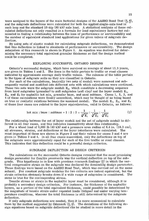
Equation 4 was established for a wide range of wheel loads P. The number of load applications N and the subgrade deflections w pertain to wheel load P. Equation 4 is also valid for the standard wheel load P., which is 9,000 lb (40 kN) (p, = 9) or for any other value within the range of the loads being investigated. If a load of P1 = 9 is ap­plied on any design section, the calculated subgrade deflection will be w,, and, with these two values, Eq. 4 will predict the number of equivalent standard axle load appli­cations N,. From these considerations, the load equivalency factor e = N,/N can be derived and was found to be

e = (:.r X 10-0.09(P-P,1 (5)

The following equation is presented for large values of z and for a constant radius of tire pressure area a= a, = constant (which is the same for P and P,):

e = (:.)6 X 10-0.09 (P - P,I (6)

(If P and P, are metric, then the -0.09 coefficient changes accordingly.) Equation 6 has been plotted in Figure 4 for P. = 9 [9,000 lb (40 kN)] together with equivalency factors derived by Shook and Chastain (8, 9). If Eq. 6 is true, it follows that the destructive effects of heavy axle loads P > P, have usually been overestimated.

PREDICTION OF EQUIVALENT STANDARD AXLE LOAD APPLICATIONS

The weighted axle load applications N2.s and N1.s (5, tables 6 and 8) were converted into numbers of equivalent standard 18-kip loads (N2~ = e x N2•5 and N1.s = e x N1.s) by using equivalency factors e calculated by Eq. 5.

N2.s and N1.s were then correlated with all the calculated deflections of loops 3, 4, 5, and 6 for cases 3 and 4. The results of these correlation regression analyses, each based on over 100 pairs of values w. - N, are as follows:

1. For case 3, p = 2.5: log N2.s = -5.93 log w. - 3.12; 2. For case 3, p = 1.5: log N1.s = -5.94 log w. - 3.06; 3. For case 4, p = 2.5: log N2.s = -5.90 log w, - 3.41; and 4. For case 4, p = 1.5: log N1.5 = -5.92 log w. - 3.35.

In all four cases correlation coefficients r""' -0.95, errors of prediction""' 0.26, 95 per­cent confidence limits of the slopes are approximately 5. 5 to 6.3, and average standard error of the slope""' 0.19. The errors of prediction(""' 0.26) compare favorably with the root-mean-square residual of the AASHO Road Test data, which is 0.31.

These correlation regression equations were then harmonized as before based on a constant slope of 6. The same equations were obtained as from Eq. 4 for P = 9 kips (40 kN). They are given in log form on the bottom of Tables 5 and 6. Plots of the points and the regression lines for cases 3 and 4 and for p = 2.5 are shown in Figures 5 and 6.

Thus, the subgrade deflection principle or model has been successfully applied to the AASHO Road Test data even with gross assumptions for the elastic moduli and layer

22

Figure 4. Load equivalency factor versus wheel load.

10-i--....L...-....L...-....L...-....L...-....L...-....L...-....L...-....L...--',--..1.---,,J---'---'----:iJ----'--+

r .. "' ~ ~

9 8 7

6

5

4-

3

2

l5·

i 1.0 ..... .9 ~ .8 ~ .7 w .6

.5

.4

.3

.2 P, , 9 KIPS

1.5 +--..-...... ,---,---..--+--..--..---,---,---,---.---,---,---,---,----4-4 5 6 7 8 9 10 11 12 13 l.d 15

Table 6. Correlation regression equations for AASHO Road Test results (p = 1.5).

Loop Axle Load Number (kips) Equations for Case 3 Equations for Case 4

3 12 log N = -4.358 log w - 1.174 log N = -4.214 log w - 1.212 4 18 log N = -5.838 log w - 2.805 log N = -5. 785 log w - 3.056 5 22.4 log N = -5. 766 log w - 2.647 log N = -5.652 log w - 2.823 6 30 log N = -5.891 log w - 2.414 log N = -5.849 log w - 2.689

Suggested predicting equation& for N = e N log Nie= -6 log w1 - 3.13 log N = -6 log w, - 3.47

Note: Measurement of wand w1 is in inches 1 in = 2.54 cm, 1 kip • 4 ,448 222 N

16 17

Sample Size

25 25 25 22

97

•standard error of prediction of log f'1 "'Q_26; standard error in slope "' 0 .20. Stcmdard error in Y-intercept "' O 59; correlation coefficient= ·0.95

18 19 20

P-

Figure 5. Verification of predicting Eq. 4 for case 3.

(J.08

0-07

0.06 X

o.os

).04

0.03

LEGEND-A Loop3,P5 =9kips,N=ewN, P=6kips X loop 4, P, = 9 kips, N= N, P= 9kips

B Loop5,P5 = 9kips,N=exN, P=ll.2kips

0 Loop6,P51: 9kips, N=e•N, P=15kips

• = 10-0.0,1,.,., ~ ) 6

X

Er 50000psi Ei= 15000 psi

E,.= 3000 psi

EQUIVALENT NUMBER OF 18 kip AXLE LOAD APPLICATIONS N. 0

o.02•-+--r---r-r..-i'"T"l-.--r-r"T'Tr---,-r-r"""T""T"1r-TI"""T""T'T'TT--r---r-r-r,rrn-..-i'"T"l-,---,r--r-r-r-rr,r---T"T"'1r'T"lr-

\OOO 10,000

'igure 6. Verification of predicting Eq. 4 for case 4.

\08

t.07

.06

0

04

1,000

'{ z 0 ;:: u ~ ~ w Cl ~

"' ~ ::,

"'

10,000

100,000

100,000

\000,000

LEGEND, A Loop 3, Ps = 9 kips, N=e KN, P=6 kips X Loop 4, P5 = 9 kips, N= N, P=9 kips

l!J Loop 5, P5 -= 9 kips,N=e•N, P=11.2kips 0 Loop 6, P5 = 9 kips, N=e xN, P=15 kips

es: 10-0.09(P-Psl•(: i6

\000,000

1),000.000

10,000,000

24

equivalencies. Equations 4, 5, and 6 and the regression equations were derived con­currently for both cases 3 and 4 with concordant results. This shows that the subgrade deflection model is not sensitive about the relation between subgrade and pavement layer moduli. From here on, investigations are restricted to case 3 as an example only.

LOSS OF SERVICEABILITY

The number of equivalent 18-kip axle load applications N for the two terminal levels of serviceability p = 2.5 and 1.5 (PSI) can be calculated by Eq. 4 by setting P = 9 kips (40 kNL This substitution leads to two expressions that have been combined into one performance equation relating N to the subgrade deflection w1 and to the loss in per­formance. With Eq. 4, and by using the K-values of case 3, by setting P, = 9 kips (18-kip axle) [40 kN (80 kN)], and by assuming an initial value of p0 = 4.2 (5), one can derive the following equation by connecting the three points Po = 4.2, Pi = 2:5, and p2 = 1.5 by a cubic parabola:

p = 4.200 - (1.22275 1/l + 4.4024 ip3) (7)

where

ip = 1000 x w: x N for w, in inches (8)

or

ip = 3.7238 w~ x N for w. in cm (9)

and where

w. = deflection on top of the subgrade as a design parameter for the standard wheel load P. = 9 kips (40 kN),

.J> = PSI, and Np = number of equivalent 18-kip (80 kN) axle weight applications.

The last term of Eq. 7 can be interpreted as the loss in PSI because of traffic loading.

PL = 1.2228 1/l + 4.402 1/>3 (10)

In this form, the predicting equation could eventually be used more universally, for instance for other initial values p0 and in other environments by including another loss term to account for additional losses from environmental forces, a concept which at present is being applied to the results of the Brampton Road Test (10, 11, 12). Figure 7 shows the losses PL as a function of N and w,. - - -

REQUIRED EQUIVALENT GRANULAR THICKNESS

Equation 2 can be solved explicitly for z, and the resulting equation, with Eq. 3, can • be multiplied by

(11)

where E2.g is the modulus for granular A base material. In this way, a design equation may be derived:

(12)

where H0 is the required granular thickness for the particular design in terms of granu­lar A material. This thickness requirement H0 is the sum of all layer thicknesses mul­tiplied by layer equivalency coefficients.

(13)

Figure 7. Loss of performance or serviceability because of traffic loading (mean values).

0

!,!

$ .. ... 12 w ::, 0 ... ~ ~ 2

i <

i 3

4 0

NUMBER OF EQUIVALENT 18 KIP AXLE LOAD APPLICATIONS N

Figure 8. Design chart for flexible pavements in Ontario.

::i :c

~ ~

~~ 0·0 3

" .. < ! 0 Q z 0 ;:: u w s 0

~ 0·02 < "' C)

"' ::,

"'

EQUIVALENT ASPHALT LAYER THICKNESS. (INS) 10 10 JO

m1ib1~ P , 9000 lb a 1 6 4 11

+ E1• 400,000 psi ;, E,• 50, 000 psi h,

+

E , l 15, 000 psi ;,

e. 1, 1500 • CBRI

dHii,, equations

H,• 1.y~-p )'-•' X ~ 0.9 2Emw1

E1

H8 •2h1 + h1 + f h3

equivalencin: 1"hot mhc • • 2"granular "A" sJ"aJbb8:18

30 40 so 60

H,• THICKNESS OF PAVEMENT IN EQUIVALENT INCHES OF GRANULAR A

GRAN. TYPE

MATERIALS

SUITABLE

ASGA~N.

BORROW

11,000

TYPICAL SUBGRAOE MODULI IN ONTARIO

iA.IIOl"lllt 1Ui'D CLA'I' LOAM TILL t!LJ c;, 6~ lfP..T ,o TJG s1Ll :>r,o 1/.F.S. 1/.F.S., 1/.F.S... .,.dSi.

6,000 TO

7,000

.,dSi .

"'·'° .. ,.ooo

TO 6,000

andSi . >,o

J,000 TO

5,000

LACUSTA INE

CLAYS

3,500 TO

6,000

VARVED AND

LEDA CLAYS

,,, 2,000

TO ,.soo

3

0.01

0.09

0.06

0.07

"' w :c u ~

0.06 ~

0 z ::,

0.05 0 "' w .. ::E < llj

0.04 z < :E

~ ~

0.03 "'

0.025

0.02

0.015

70

25

\'.)

~ "' 0..

"' ~ V, ... z w Nj ::E w

"' 0 ::, ... "' + <t w r ::E

c,. "' ci .,: w

GO 0..

0 uJ ::,

~ z .,: uJ ::E

26

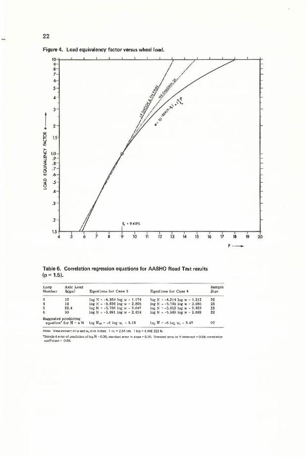
These coefficients express the effect of each layer in resisting load P. to generate a vertical deflection w. on the subgrade, which is the design parameter. Therefore, they are (as in Eq. 3) related to the pavement layer moduli as follows:

C1 = ~ C2=~ Cs=~ E21 E2g Es, (14)

In this paper, coefficients were based on exper ience gained in Ontario, especially from the Brampton Road Test results (10): C1 = 2, c2 = 1, and cs = %. TJ1ey determine the relation E1:E2 :Es of the pavement layer moduli (Eq. 1) within the subgrade deflec­tion concept (Eqs. 2 and 3). In other words, the pavement layer moduli were based on layei l -tuivalencies determined from experience. This is justified if the perfor­mance is linked to the subgrade deflections w calculated by Eqs. 2 and 3. [The similarity of desig.1 Eqs. 12 and 13 with the Kansas formula (13, 14) is recognized.]

A design chart for determining the required totalthickness in terms of H. was drawn with Eq. 12 and is shown in Figure 8. The following example may show how to use the chart. The assigned Odemark subgrade deflection is w. = 0.019 (to be taken from a suitable performance diagram similar to Fig. 7). The subgrade is a clay loam till with 30 per cent silt and with very fine sand and silt of about 40 percent; therefore, select Em = 6,000 psi (41. 4 MPa) from the table in Figure 8. The required granular A thick­ness from the same figure is H& = 21 in. (53 cm>.

CONCLUSIONS

A practicable system of flexible pavement design, which is a subsystem of the whole pav:ement management system, can be based on simple concepts of linear elastic theory. An elastic layer system can serve as a structural design pavement model. The sub­grade deflection for this model was found to be the most relevant distress indicator for the loss of performance of the pavement as a whole. The link between the response of this model, in terms of vertical deflections on the subgrade, and the output function, in terms of loss of performance, was established by considering past experience with successful Ontario designs and the AASHO Road Test.

The material characterizations and load applications of the input variables of this model, although not definitely established, were demonstrated and exemplified. Thus, experiences in Ontario were mainly used to establish realistic relations between layer and subgrade moduli, and AASHO Road Test data were used to exemplify the necessary range of loads.

REFERENCES

1. Phang, W. A., and Slocum, R. Pavement Decision Making and Management System. Ministry of Transportation and Communications, Ontario, Rept.- RRl 74, Oct. 1971.

2. Dormon, G. M., and Edwards, J. M. Shell 1963 Design Charts for Flexible Pave­ments, An Outline of Their Development. Shell International Petroleum Co. Ltd., London, O.P.D. Rept. 232/64M, April 1964.

3. Odemark, N. Investigations as to the Elastic Properties and Soils and Design of Pavements According to the Theory of Elasticity. statens Vaeginstitut, stockholm, 1949.

4. Shook, J. F., and Finn, F. N. Thickness Design Relationships for Asphalt Pave­ments. Proc., International Conference on the structural Design of Flexible Pave­ments, Univ. of Michigan, Ann Arbor, Aug. 1962, p. 52.

5. The AASHO Road Test, Report 5: Pavement Research. HRB Special Rept. 61 E, 1962.

6. The AASHO Road Test, Report 6: Special Studies. HRB Special Rept. 61 F, 1962. 7. Evaluation of AASHO Interim Guides for Design of Pavement Structures. NCHRP

Rept. 128, 1972. 8. Schnitter, G., and Jentasch, R. J. Designing Flexible Road Pavements. Proc.,

International Conference on the Structural Design of Flexible Pavements, Univ. of Michigan, Ann Arbor, Aug. 1962, p. 537.

27

9. Secor, K. E., and Monismith, C. L. Viscoelastic Properties of Asphalt Cement. HRB Proc., Vol. 41, 1962, pp. 299-320.

10. Kamel, N. I., Morris, J., Haas, R. C. G., and Phang, W. A. Layer Analysis of the Brampton Test Road and Application to Pavement Design. Highway Research Record 466, 1973, pp. 113-126.

11. Phang, W. A. Four Years' Experience at the Brampton Test Road. Ministry of Transportation and Communications, Ontario, Research Rept. RR153, Oct. 1969.

12 . Phang, W. A. The Effect of Seasonal Strength Variation on the Performance of Selected Base Materials. Ministry of Transportation and Communications, Ontario, Research Rept. IR39, April 1971.

13 . De Barros, S. T. A Critical Review of Present Knowledge of the Problem of Rational Thickness of Design of Flexible Pavements. Highway Research Record 71, 1965, pp. 105-128.

14. Yoder, E. J. Principles of Pavement Design. John Wiley and Sons, New York, 1959.

15. Szechy, K. Der Grundbau, Vol. 1. Springer-Verlag, Vienna, 1963, p. 249.

APPENDIX DESIGN FORMULA BASED ON SUBGRADE DEFLECTIONS

A design formula based on subgrade deflections can be derived by using various ex­isting concepts such as the solution of an elastic stress anal ysis for the isotropic half space and the equivalent layer thickness suggested by Odemark (3, 8).

Newmark (15) gives a formula for the vertical deflection in the center of a wheel load that is equally distributed over a circular contact area at depth z of a uniform elastic half space.

( ) a a ~ . ( ) 1 - cos aJ w • = 1 + µ X Eo X srn Ct + 1 - 2µ . sin Ct

where

w. = vertical deflection at the top of the subgrade; µ = Poisson's ratio;

r:1 0 = tire pressure, uniformly distributed over a circular area; a = radius of the loaded circular area; a = angle as indicated in the figures; and

a = arc tan ~. z

Equation 15 is rewritten so that an important simplification can be achieved:

(15)

28

K C7o a . w, = xEx sma (16)

where

K =; (1 + µ.) rcl - 2µ.) X 1 -. c2os a] r sm a (17)

Forµ. = 0.25 to 0.50 and for ex= 0 to 40 degrees the coefficient varies only slightly from K = 1.5 to K = 1.6, and a constant value can be selected. In particular, the coef­ficient K increases slightly by decreasing Poisson's ratio (µ. < O. 5) and by increasing a.

A fixed value of K = 1.5708 = i- > 1.5 is suggested.

For a Poisson's ratio ofµ. = 0.5, Eq. 15 is simply

1 5 a.ax . w 1 = • XE sma (18)

This is a well-known equation (2, 3, 4). By referring to Eq. 16, the following substitution can be made - - -

. tana t a dP 2 sin Qt = , an QI = z' an = fr a (7 o

../1 + tan2 a

w = KP X---1 __ _ 1

rrEz ~

Solving for z,

Z =v't1r ~~s -a2

K 1 where P = design wheel load = 1r a2 a., and rr = 2.

Figure 9. Diagram of elastic layered system. 1 -a

CONTACT STRESS 0-0

\ I

e11UViEN-eouND LAYERs ' ' \ a LI (MODULUS E1) ~

\

I I

GRANUlAR BASE AND SUBBASE

( MODULUS E2) r'a,/ ..,, I

'I I

I I

I I

I I

I I

SUBGRADE (MODULUS Em )

SUBGRADE DEFLECTION

(19)

(20)

29

According to Odemark (3), an elastic layered system as shown in Figure 9 can be transformed into a uniform-elastic half space by introducing an equivalent layer thick­ness h..1,

where

E1 = modulus of layer i, E. = modulus of subgrade = reference modulus, h1 = thickness of layer i,

he1 = equivalent thickness of layer i, and n = reduction factor, for flexible pavements = 0,9.

(21)

For flexible pavements, Odemark (3) has suggested a value of n = 0.9. This was veri­fied by numerous comparative calculations.

The depth z can be expressed by Eq. 21 as

m-1 m-1

z = I h.1 = n I h1 ~ (22>

i=l i=l