Eindhoven University of Technology MASTER Target height ... · monopulse radar. The monopulse...
88
Eindhoven University of Technology MASTER Target height estimation in multipath using monopulse complex angle van de Meerakker, J.C.H. Award date: 1998 Link to publication Disclaimer This document contains a student thesis (bachelor's or master's), as authored by a student at Eindhoven University of Technology. Student theses are made available in the TU/e repository upon obtaining the required degree. The grade received is not published on the document as presented in the repository. The required complexity or quality of research of student theses may vary by program, and the required minimum study period may vary in duration. General rights Copyright and moral rights for the publications made accessible in the public portal are retained by the authors and/or other copyright owners and it is a condition of accessing publications that users recognise and abide by the legal requirements associated with these rights. • Users may download and print one copy of any publication from the public portal for the purpose of private study or research. • You may not further distribute the material or use it for any profit-making activity or commercial gain
Transcript of Eindhoven University of Technology MASTER Target height ... · monopulse radar. The monopulse...

Eindhoven University of Technology
MASTER
Target height estimation in multipath using monopulse complex angle
van de Meerakker, J.C.H.
Award date:1998
Link to publication
DisclaimerThis document contains a student thesis (bachelor's or master's), as authored by a student at Eindhoven University of Technology. Studenttheses are made available in the TU/e repository upon obtaining the required degree. The grade received is not published on the documentas presented in the repository. The required complexity or quality of research of student theses may vary by program, and the requiredminimum study period may vary in duration.
General rightsCopyright and moral rights for the publications made accessible in the public portal are retained by the authors and/or other copyright ownersand it is a condition of accessing publications that users recognise and abide by the legal requirements associated with these rights.
• Users may download and print one copy of any publication from the public portal for the purpose of private study or research. • You may not further distribute the material or use it for any profit-making activity or commercial gain
Eindhoven University of TechnologyFaculty of Electrical EngineeringDepartment Measurement and Control Systems
Target heigllt estimationin multipath using
monopulse complex angle
JCH van de Meerakker
Report of the graduation project done by J.C.H. van de Meerakker at HollandseSignaalapparaten B.V. in Hengelo.Date: 1 september till 1 march 1998Supervisor Signaal: 1.K. BrouwerSupervisors TUE: prof. dr. ir. P.P.J. van den Bosch, ir. Y. Boers
The faculty of electrical engineering of Eindhoven University of Technology does not acceptany responsibility for the contents of traineeship- or graduation reports.
Target height estimation in multipath using monopulse complex angle
Summary
When a monopulse radar is tracking a low elevated target, multipath effects disturb the targetheight measurement. Various ways exist to estimate the target height under these circumstances.
In this paper a method is studied to estimate the target height using the complex angle of themonopulse ratio. This method consists of applying a transmitter frequency change and measuring the resulting phase change of the monopulse ratio. From these data the target height can becalculated.
Various error sources have been modelled and simulated:
• Antenna mispointing will in some situations cause loss of track. A way is derived to sayfrom a measurement whether or not it is susceptible to tracking divergence. In theory tracking divergence can often be avoided by choosing the appropriate transmitter frequencies.
• Glint will cause severe height measurement errors when the target is large.
• Diffuse reflection will cause errors at targets with high elevation and at high sea states.
• Quantisation noise is not a large source of error, due to the processing that is done in theMTTU.
• Phase imbalances between the receiver channels may cause systematic errors in the estimated target height. An experiment is proposed to investigate how large these phase imbalances are and how they vary with transmitter frequency, time and temperature.
The effect of glint, diffuse reflection, quantisation noise and phase imbalances can be reducedby making the applied frequency step larger. A restriction is that the measured phase changeshould not be larger than 1t, or else ambiguities will occur. Also, areas where mispointingcauses tracking loss should be avoided.
Low target measurements done at sea in 1991 have been used to test the method. Since themeasurements were taken at sea state 4, diffuse reflection is expected to cause severe errors onthe estimated target height. In the F-16 runs, the estimated target height is very noisy. In theRushton runs in some intervals the correct target height is found with a RMS error of 5 meters.Unexplained spikey areas remain.
If problems like phase imbalances are solved, measuring target height with the complex angleof the monopulse ratio may be useful for small, low flying targets at smooth sea.
It is recommended to perform tests to investigate phase imbalances, to investigate the mispointing effects and to test the complex angle method on low target measurements at smoothsea.

Target height estimation in multipath using monopulse complex angle
Samenvatting
Ais een monopulsradar een laagvliegend doel voIgt, wordt de doelshoogtemeting verstoorddoor multipad-effecten. Er bestaan verschillende manieren om onder deze omstandighedentoch de doelshoogte te meten.
In dit rapport wordt een methode onderzocht die de doelshoogte bepaalt met behulp van decomplexe hoek van het monopulsquotient. De methode bestaat eruit, dat een verandering in dezendfrequentie wordt aangebracht en dat de resulterende verandering van de fase van hetmonopulsquotient gemeten wordt. Uit deze data kan de doelshoogte berekend worden.
Verschillende foutenbronnen zijn gemodelleerd:
• Antenne mispointing zal in sommige situaties doelverlies opleveren. Een manier is afgeleidom uit gemeten waarden te concluderen of de desbetreffende meting zalleiden tot doelverlies. In theorie kan doelverlies vaak vermeden worden door geschikte zendfrequenties tekiezen.
• Glint veroorzaakt ernstige fouten in de gemeten hoogte als het doeI groot is.
• Diffuse reflectie veroorzaakt meetfouten bij doelen met hoge elevatie en bij hoge zeegang.
• Quantisatieruis is geen belangrijke bron van fouten, daar bij de dataverwerking in de MTTUeen groot gedeelte weggefilterd wordt.
• Faseongelijkheden tussen de verschillende kanalen in de ontvanger kunnen systematischefouten veroorzaken in de gemeten doelshoogte. Een experiment is voorgesteld om in kaartte brengen hoe groot deze faseongelijkheden zijn en hoe ze afhangen van de zendfrequentie,tijd en temperatuur.
Ret effect van glint, diffuse reflectie, quantisatieruis en faseongelijkheden kan verminderdworden door de toegepaste zendfrequentiestap groter te maken. Een beperking hierbij is, dat degemeten faseverandering niet groter mag zijn dan 7t, anders treden dubbelzinnigheden op.Tevens moeten gebieden waar mispointing doelverlies veroorzaakt vermeden worden.
Laagdoelmetingen, die in 1991 op zee gedaan zijn, zijn gebruikt om de methode te testen. Vanwege de hoge zeegang tijdens de metingen, sea state 4, werd verwacht dat diffuse reflectie ernstige fouten zou veroorzaken in de geschatte hoogte. Bij de F-16 metingen bevat de geschattehoogte veel ruis. Bij de Rushton metingen is op sommige intervallen de goede doelshoogtegevonden met een standaarddeviatie van 5 meter. In de metingen zijn gebieden waar omonverklaarde redenen veeI uitschieters op de gemeten hoogte zitten.
Ais problemen zoals faseongelijkheden opgelost zijn, kan doelshoogtemeting met de complexehoek van het monopulsquotient zinvol zijn voor kleine, lage doelen op rustige zee.
Ret is aan te bevelen, tests te doen om de faseongelijkheid te onderzoeken, om het effect vanrnispointing te onderzoeken en om de methode te testen bij rustige zee.

Table of Contents
1. Introduction 51.1. Monopulse radar 51.2. Multipath 81.3. Solutions to the low target problem 101.4. Objectives 11
2. Description of the low target problem 122.1 Reflection at the sea surface 122.2 Multipath geometry 132.3 Monopulse measurement in multipath 142.4 Measuring target height. 17
3. Sources of errors 213.1. Antenna mispointing 213.2. Noise on phase S 253.3. Glint 283.4. Quantisation noise 303.5. Diffuse reflection 33
4 Phase calibration of the STING-EO 384.1. Experiment 39
5. Target height measurements from real data 405.1. Processing 415.2. Results 425.3. Conclusions 49
6. Algorithm tuning 506.1. Choice of transmitter frequencies 506.1.1. Selecting the optimal frequency step 516.1.2. Finding a frequency range without mispointing divergence 526.2. Antenna control 57
7.1. Conclusions 597.2. Recommendations 60
Literature 62
Appendix A1 SymbolsAppendix A2 Integration of three measurementsAppendix A3 Derivation of 'YAppendix A4 Error in found target height due to mispointingAppendix A5 Coordinate systems round earth
Appendix B ListingsAppendix B 1 The simulatorAppendix B2 Processing registered measurements

5 Target height estimation in multipath using monopulse complex angle
1. Introduction
Monopulse radar is a widely used technique for measuring the location of a target. As it allowsaccurate measurements of the angular location of a target it is commonly used for tracking andfire control purposes.Unfortunately, monopulse radar suffers severe degradation in the case of multipath, when thetarget position is near the earth surface. The standard monopulse radar measures the target elevation with severe errors in this case. Different ways to deal with this problem are described inliterature, varying from filtering techniques to hardware solutions such as extra receiver channels. In this report a study is described on a technique that makes use of the complex angle ofthe monopulse quotient. After a theoretical description of the low target problem an algorithmfor measuring target height using the complex angle is described in chapter 2. In chapter 3 theinfluence of different error sources on the measured target height is investigated. When usingthe complex angle an accurate calibration of the phase error between t1 and L channel is necessary. In chapter 4 an experiment is described to investigate how this phase error changes asfunction of frequency, time and temperature. Target height measurement with complex anglefrom measured data are described in chapter 5. In chapter 6 the choice of the transmitter wavelengths and some demands on antenna control are described. In chapter 7 conclusions aredrawn about the conditions under which target height measurement with complex angle maybe useful and recommendations are given on further research.
1.1. Monopulse radar
Monopulse is a method of measuring the angular location of a source of radiation or of anobject that reflects radiation that is incident on it. The technique is used in many fields, forexample in astronomy to measure the position of radiating objects. It is also used in radar sincethe 1940s. Monopulse radar is nowadays widely used for precise angle measurement andtracking. [Sherman84] and [Leonov86] give a detailed explanation on the principles ofmonopulse radar. The monopulse technique is based on comparison of signals received by different antenna patterns. Different implementations exist. In this section the working of a common type of monopulse radar, the four feedhorn amplitude comparison monopulse radar, isdescribed.
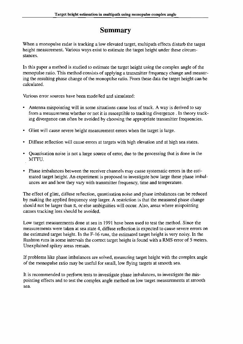
The basic principle of monopulse can best be understood by considering the situation of picture 1.1. The radar has two radar beams with a slightly different elevation angle. A radar pulseis transmitted on both beams at the same time and the reflection is measured. The differencebetween the voltage measured by the upper and the lower beam gives information on the elevation angle of the target with respect to the antenna axis, which is in monopulse radar usuallycalled boresight axis. See picture 1.3. for a definition of azimuth and elevation. if VI-V2 >0 the
target is above the boresight axis, if VI-V2 <0 the target is beneath the boresight axis and if
V1=V2 the target is on the boresight axis.The sum L= V1+V2 and the difference t1=V1-V2 are
plotted as function of elevation angle in picture 1.2. To make the measurement independent ofthe power of the reflected signal, the difference can be divided by the sum. This quotient iscalled the monopulse quotient. As can be seen from picture 1.2 the monopulse quotient is
Chapter 1. Introduction 6
approximately a linear function of angle for angles within the beamwidth. In practicalmonopulse systems a correction is done to make it a linear function of angle till approximatelyhalf the beamwidth of the sum beam.
VI = voltage from upper beamV2 = voltage from lower beam
Picture 1.1. Monopulse principle
1.5,-------r--....---,------r--....---,------r-----r....---,-----,
EIII<ll.cE::J
C/)-o~ 0.5 ..III<ll0.o-"0<ll.~ o·"iiiEoc:uiE -0.5<ll
~0.<llClIII.g -1>
-0.8 -0.6 -0.4 -0.2 0 0.2 0.4 0.6 0.8angle, normalized to Sum-pattern bandwidth
Picture 1.2. Antenna pattems amplitude comparison monopulse
The two beams of picture 1.1 measure the elevation angle. To measure also the azimuth angle,usually an antenna with four beams is used. A parabolic reflector is fed by a cluster of fourfeedhoms that are placed next to each other as in picture 1.4. A cross section of the beams isdrawn in picture 1.5. Note that due to the reflection at the paraboloid the beams are on the

7 Target height estimation in multipath using monopulse complex angle
opposite side of the boresight axis as the feedhorns. From signals received by the four feedhorns the L, ~E (elevation) and ~A (azimuth) signals are formed according to
North x
1L = 2:(A + B + C + D)
1= 2:((C+D)-(A+B))
1~E = 2:((A + C) - (B + D))
z
(1. I-a)
(lJ-b)
(1.1-c)
y
focal planeI
feed horns~waveguides boresi ht axis
------------g---~
a. Side view
Picture 1.4. Reflector and feed horns
~~
b. front view feedhorns
Picture 1.5. Cross section monopulse beams
For transmitting the radar pulse the same antenna is used as for receiving the echo. The fourfeedhorns transmit the same pulse, which has therefore the shape of the sum pattern of picture1.2. When receiving the echo the signals L, ~E and ~A are measured. The monopulse quotient
~EIL is proportional to the elevation angle of the target with respect to the boresight axis, the
monopulse quotient ~AIL is proportional to the azimuth angle.

Chapter 1. Introduction
1.2. Multipath
8
If a target is above a surface that reflects radar waves, such as the sea, the radar signal that isreflected by the target will not only travel through the direct path, but will also arrive via thereflecting surface. Thus, the radar receives two signals instead of one. This effect is called multipath.
The indirect path will be longer than the direct path. This way length difference causes a phasedifference between the two signals. Depending on this phase difference, the signals will interfere with each other. If they have equal magnitude, for example when reflecting at smooth sea,and opposite phase, they may cancel each other completely, causing the radar to lose track ofthe target.
This small received signal strength due to destructive interference is a problem for all types ofradar. Additional to this, monopulse radars suffer from the fact that receiving signals frommore than one direction, makes the monopulse measurement of target angle virtually worthless. This can be understood by looking at picture 1.6, in which the direct signal, the indirectsignal and the total signal as received by a monopulse antenna are drawn in the complexplane.The receiver measures a sum signal L and a difference signal ~E' These signals can be
thought of as being the sum of the signals that come from the target and from the mirror. L t
and Lm are the sum signals from respectively the target and the mirror, ~t and ~m are the difference signals. In this example L t and ~ t are in phase, because the target is above the boresight
axis. L mand ~m are in opposite phase, because the mirror image is beneath the boresight axis.Due to the way length difference and a phase shift at the mirroring point, there is a phase difference 'Pt between the direct and the indirect path. The sum and difference signal measured by
the radar will have a phase difference 'Ps' This phase difference need not be 0 or 1800 as is thecase in the free-space situation, but can have any value, depending on the position of target and
antenna.
1m
~E
~m"-
"-"-
"- L Re
Picture 1.6. Received signal in multipath
9 Target height estimation in multipath using monopulse complex angle
When L t and Lm have opposite phase and are of almost equal magnitude, the resulting L will
be very small. In that case, the real part of the complex monopulse quotient !lEIL will be very
large, leading to a far too large measurement of the target elevation angle. When L t and Lm are
in phase, the real part of !lEIL will be too small, leading to a too small measurement of the tar
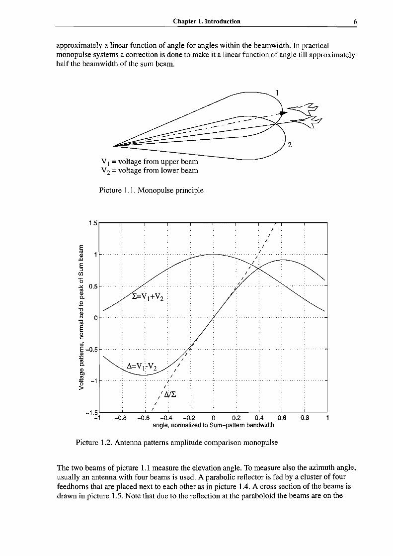
get elevation angle.The target height that a monopulse radar would measure in the case of multipath as function of the range is given in picture 1.7 for different values of the reflectioncoefficient of the sea surface p.
45
40 .......... • t • • • • • 'p'==O...8. . . . . ~ . . . . . ... .....
35 .......... . . . .
30 ......... . . . . . . . . .
,......,E 25........'ijlI)I-< 20::3enCdlI)
E 15
..c10
5
0 .........
-50 1 2 3 4 5 6
R [km]
Picture 1.7. Simulated monopulse measurement of the target height in the case of multipath
target height ht=5 m, antenna height ha=10m, transmitter wavelength 1..=0.0333 m,beamwidth=38 mrad, p=O, 0.2, 0.4, 0.6, 0.8
As can be seen from picture 1.7, multipath renders the target height measurement of amonopulse radar virtually worthless. The problem is most important when the target is lowabove the sea surface, for two reasons:
1. the target is near to its image, so that the antenna gain in the direction of the target is moreor less the same as in the direction of the image.
2. The reflection coefficient p is larger when the grazing angle, the angle at which the reflectedEM-wave incides at the sea surface, is lower, id est when the target is closer to the sea.
Because of this, the problem is also called the low target problem.

Chapter 1. Introduction
1.3. Solutions to the low target problem
10
The low target problem has been known since the 1960's and a number of solutions have beenproposed in the past. In this section, a short review is given of some of these solutions, withoutgoing too much into mathematical details.
Keeping the beam outside the mirror.
By making sure that the antenna gain in the direction of the virtual target is always small, theindirect signal will be eliminated or at least reduced. Practical implementations of this principle vary from pointing the antenna above the target, so that the beam does not touch the sea, tousing special beams that have a high beamwidth in azimuth and a small beamwidth in elevation[SHERMAN84],[MAAS97]. In phased array antennas it is possible to put a zero in the antennapattern in the direction of the virtual target.
Low target filter
As can be seen in picture 1.6, the measured target height has peeks and valleys around the realtarget height. Making use of a changing target range a low pass filter may be applied to get abetter height estimate. This has been done in the past, and it is used in commercial systemsnowadays. However, the accuracy of the method is low, and the method needs a target thatmoves towards or from the radar, preferably at high speed [ROTGANS88].
Nonsense channel
This method consists of the use of the diagonal of the monopulse cluster. In additional to the~E and ~T channel an extra channel is implemented as (A+D)-(B+C), the so called nonsense
channel (see picture 1.5). This channel has a wide zero in the direction of the antenna axis. Ifthe antenna is directed to the target, the nonsense channel will only receive energy of the virtual target. Using this information, the disturbance of the virtual target can be eliminated.[SHERMAN84], [ROTGANS88].
Complex angle
The phase difference CPt between direct and indirect signal depends on the wavelength and on
geometrical parameters like target range, antenna height and target height. This phase difference causes a phase shift CPs between ~ and L channel, as can be seen in picture 1.6. Thus, by
measuring CPs at different wavelengths theoretically the target height can be found. In this
report a method to do this will be treated in more detail.

11 Target height estimation in multipath using monopulse complex angle
1.4. Objectives
In the past, methods to estimate the target height using the complex angle have been devised([Sherman 71], [Sherman 84],[Symonds 73]) and experiments on the matter have been done([Howard 74]). [Nakatsuka 90] and [Wang 96] describe the use of complex angle with theantenna pointed midway between target and mirror target. At Signaal research is done onapplication of complex angle with the antenna pointed at the target. Tests have been done onthe matter in 1991, with negative results [Setyowati 92]. However, people at Nobeltech [Eckersten 92], reported to have an implementation of complex angle that performs well in a testenvironment.
In this report a further investigation on low target algorithms based on the complex angle isdone. Objective is to find out which are the factors that limit accuracy and to investigate whichdemands should be put on the radar hardware and control components to get the necessaryaccuracy.
Questions that we intend to answer are the following:
What is the influence of the different measurement errors on the found target height?• Inaccurate measurement of phase <Ps between L1 and L• Inaccurate initial estimation of the target height• Error in range, wavelength, antenna height• quantisation noise in the receiver
What is the influence of deviations from assumptions made in the model?• diffuse reflection• glint
What demands should be put on the hardware? (transmitter, receiver, antenna)
What demands should be put on the radar control? (wavelength and wavelength program,antenna control)
Chapter 2. Description of the low target problem
2. Description of the low target problem
12
(2.1)
When a target measured by a radar is close to a surface that reflects radar waves, the radarmeasurement will be corrupted by multipath interference. In this section, a description is givenof the multipath effect in the case of a monopulse radar and a target close to the sea surface. Insection 2.1 the reflection at the sea surface is discussed. In section 2.2 the used point mirrormodel is established. According to this model, radar waves between the target and the antennatravel along two different paths, the direct path and the indirect path. The length differencebetween the two paths introduces a phase difference between the two received signals. It isderived how this phase difference depends on the position of target and antenna. In section 2.3is described how the signals measured with a monopulse radar depend on the phase differencebetween the radar waves travelling through the direct and indirect path, on the reflection coefficient and on antenna parameters. In section 2.4 is derived how the target height can be measured using the phase of the monopulse ratio.
2.1. Reflection at the sea surface
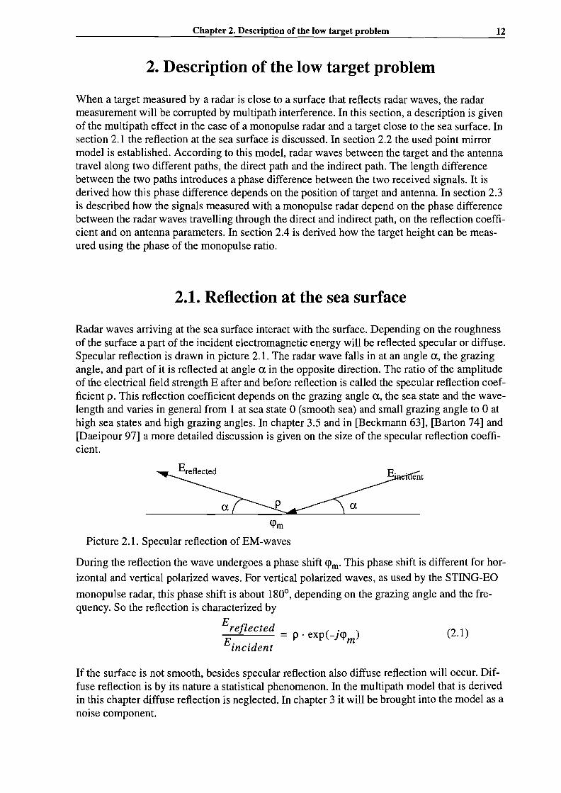
Radar waves arriving at the sea surface interact with the surface. Depending on the roughnessof the surface a part of the incident electromagnetic energy will be reflected specular or diffuse.Specular reflection is drawn in picture 2.1. The radar wave falls in at an angle a, the grazingangle, and part of it is reflected at angle a in the opposite direction. The ratio of the amplitudeof the electrical field strength E after and before reflection is called the specular reflection coefficient p. This reflection coefficient depends on the grazing angle a, the sea state and the wavelength and varies in general from 1 at sea state 0 (smooth sea) and small grazing angle to 0 athigh sea states and high grazing angles. In chapter 3.5 and in [Beckmann 63], [Barton 74] and[Daeipour 97] a more detailed discussion is given on the size of the specular reflection coefficient.
ent
a p a
<PmPicture 2.1. Specular reflection of EM-waves
During the reflection the wave undergoes a phase shift <Pm' This phase shift is different for hor
izontal and vertical polarized waves. For vertical polarized waves, as used by the STING-EO
monopulse radar, this phase shift is about 180°, depending on the grazing angle and the frequency. So the reflection is characterized by
Ereflected (.)-=-..::......-_- = p. exp -J<P
E. 'd mmCl ent
If the surface is not smooth, besides specular reflection also diffuse reflection will occur. Diffuse reflection is by its nature a statistical phenomenon. In the multipath model that is derivedin this chapter diffuse reflection is neglected. In chapter 3 it will be brought into the model as anoise component.

13 Target height estimation in multipath using monopulse complex angle
2.2. Multipath geometry
The phase difference between the signals received through the direct and indirect path in multipath depends on the geometry. In this section this relation is derived. The multipath situationaccording to the point mirror model is as in picture 2.3:
--_-Rah -.9[=----
ht
R --/~t ----.- II------ .-'- h
_----- .-'- I,tm- - - ...........- .- .- '-u Rth _ ~_r+
~--- '" Ih- - _ Ilhth I tm
I __~
Picture 2.3. Multipath geometry
In this picture the symbols are the following:ha, ht = Antenna height and target height with respect to the earth surface
ham' htm = Antenna height and target height with respect to the plane of reflection
hah, hth = Height of the plane of reflection near the antenna and near the target
u = grazing angleA=radius of the earth
Usually the antenna height ha and (an estimation of) the target height ht are known.We can cal
culate the antenna and target height with respect to the reflecting plane using the formulas (2.2a) and (2.2-b). These formulas are derived in appendix AS.
(2.2-a)
(2.2-b)
We are interested in the length difference d between the direct and the indirect path. FromPytagoras' theorem follows:
Chapter 2. Description of the low target problem 14
=(Rah + Rth)2 + (htm + ham)2
=(Rah + Rth)2 + (htm - ham)2
(2.3)
Because the elevations are low d«Rt so that d2 can be neglected. For the range difference d
can then be found:
And for the phase difference <Pt between the direct and indirect signal follows
(2.5)
<Pm is the phase shift that occurs in the reflection. The last formula gives the relation between
the geometric situation and the phase difference <Pt between the direct and indirect signal. More
in particular, it gives the relation between the target height htm above the reflecting surface, in
which we are interested, and the phase difference <Pt.
2.3. Monopulse measurement in multipath
In this section a closer look is taken at the quantities that are measured with a monopulse radar.More in particular, the relation is investigated between measurable quantities, like the real part,imaginary part and phase of the monopulse ratio and parameters of the multipath situation likethe reflection coefficient and the phase difference between the direct and indirect path.
In the case of multipath, the complex value of the sum and difference channel is given by thefollowing formulas:
(2.6-a)
(2.6-b)
In which:
Gs , GE E R = Antenna pattern of the Sum and Elevation channel (L and ~ in picture 1.2)
8 t =the angle between the target and the boresight-axis
15 Target height estimation in multipath using monopulse complex angle
8m = the angle between the mirrored target and the boresight-axis
p =The reflection coefficient of the reflecting surface<Pt =The phase difference between direct and indirect received signal
The monopulse ratio S is defined by:L1
S= -E CL
We can define an error voltage FE(8) as the monopulse ratio that would occur in the situation
without multipath with a target under angle 8. This error voltage is given by:
GE(8)F E(8) =Sfreespace =G
s(8) E R (2.7)
We will derive the monopulse ratio S as function of the error voltage in the direction of the target and the error voltage in the direction of the mirrored target. In the case of multipath Scanbe written as
(2.8)
Make the following definitions:
(2.9-a)
(2.9-b)
(2.9-c)
The error voltage T is the error voltage FE(8 t) that would be measured if only the target were
there, whereas M is the error voltage FE(8m)that would be measured if only the mirror imagewere there.
Chapter 2. Description of the low target problem 16
The effective reflection coefficient G gives the ratio between the strength of the sum signal proceeding from the mirror image and the sum signal proceeding from the target.
After substitution we find for S:
T+GMe-JCfJtS= . E C
1+ Ge-JCfJt
This can be rewritten as
Ge-JCfJtS = T-(T-M)· .
1 + Ge-JCfJt
This is to be separated in its real and its imaginary part.
(2.10)
(2.11)
Ge-Nt=
I + Ge-JCfJt
Ge- JCfJt 1 + GeNt=
1 + Ge-Nt 1 + GeNt=
G(cos<Pt-jsin<Pt + G)2
1 + 2Gcos<Pt + G
The real part of S is
and the imaginary part is
Re(S)
2Gcos<Pt + G
= T-(T-M)· 21 + 2Gcos<Pt + G
(2.12)
Im(S)Gsin <Pt
= (T -M)· 21 + 2Gcos<Pt + G
(2.13)
The phase of S is given by
<Ps = arg(S) = atan(~:gn (2.14)
17 Target height estimation in multipath using monopulse complex angle
2.4 Measuring target height
In this section a method to measure the target height is presented, based on the multipath model.The method is based on the following principle: the transmitter wavelength is changed and thechange of target range in the same time is measured. The resulting change in the phase of themonopulse ratio is measured. This change in phase depends amongst others on the target height.So if we know the magnitude of the change in transmitter wavelength, target range and phaseof the monopulse ratio, the target height can be calculated, as is shown in this section.
Theoretically it is possible to use only the change of target range and the resulting change inphase of the monopulse ratio to calculate the target height. However, the speed of targets we areinterested in, like missiles and aeroplanes, is too low to cause enough phase change in a shorttime. So a long time would be needed to make a measurement. This is not desirable because thetarget height and antenna height may change in this time. By changing the transmitter frequency, we can easily induce a larger phase change in a short time. To take both the change in targetrange and the change in transmitter wavelength into account, in the following derivation the target range and the transmitter wavelength are taken as one variable ~ according to:
~=R At
First let us take a look at the relation between the applied change in wavelength and target rangeand the resulting change in phase of the monopulse ratio.
(2.15)
in whichLl<Ps = phase change of the monopulse ratio S<Pt = phase difference between direct and indirect signal
Derivation of d<Ps/d<Pt
d<Ps/d<Pt follows from (2.14). If we assume the antenna to be pointing at the target, the error voltage T from the target direction is zero. Under this assumption we can calculate d<Ps/d<Pt:
When T is zero the real part of the monopulse ratio reduces to
2Gcos<Pt + G
Re(S)IT=o = M· 21+ 2Gcos<Pt + G
(2.16)
Chapter 2. Description of the low target problem
and the imaginary part reduces to
Gsin<PlIm(S)IT=o = -M· 2
1 + 2GcOS<P, + G
The phase is
<PSIT = 0= atan(~:~~))) = atan( -Gsin<p, 2JGCOS<P, + G
And d<Ps/d<Pt equals
2d<ps _ GCOS<P, + G- -1d<p, - 1 + 2GcOS<P, + G2
(2.17)
(2.18)
(2.19)
18
In the second tenn of the right hand part Re(S)IT=o can be recognised except for a factor M. So
d<ps = Re(S) _ 1d<p, M
(2.20)
The interesting thing about this approximation is that it consists only of elements that can bemeasured or are already known. Re(S) can be measured and M is an antenna parameter, depending on the mirror image angle, that can be calculated using an estimation for the target height.
Derivation of d<Pld~d<Pld~ follows from (2.5) to be
Isolating target heightFilling in d<Ps/d<Pt and d<Pld~ in (2.14) gives
~2 41th h~<P = J(1 - Re(S)) . am tmd~
S M ~2~l ~
Under the assumption that the target height is constant htm can be isolated, giving
(2.21 )
(2.22)
19 Target height estimation in muItipath using monopulse complex angle
(2.23)
Implementation
In practical measurement situations we can not do an infinite number of measurements. So theintegral in formula (2.23) has to be approximated from a few measurements.
Let us call the integrand A
41thA = (1 _Re(S») . am
M ;2(2.24)
The different parts of A are known or can be measured. We can approximate the integral of Afrom measurements.
Two measurements:
Three measurements, assuming that;2 is the mean Of;l and ;3:
S3
fAl+4A2+A3
Ad;z .~;6
SI
(2.25)
(2.26)
Three measurements in general:The integration can be done by fitting a parabola through the measurement points. The derivation is done in appendix A2.
Having approximated the integration, with the result the target height can be calculated using(2.23).
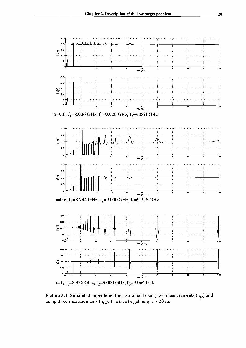
To compare the different methods, target height measurements have been simulated for differentvalues of the reflection coefficient p and for different sizes of the frequency interval. The resultsare plotted in picture 2.4. It appears that with three measurements errors are smaller than withtwo measurement. This is as expected, since with three measurements the integral is better approximated. However, with three measurements we still have some disturbance if the frequencies are far apart or if p is close to unity.
Chapter 2. Description of the low target problem 20
25,······· '.--
20 r' 'l"'I-olAl"WI~Il.,l..II.wIlwlhJ\rI.'-.j.ft\,-.~·IIA__-,-:J.I\\__::J~",----'--- ----:-__---'-__--'--_--'
.s'5f-.·
~ 'Or"
5~o0~L-L-----'----2~-~3---4'---~5---6'-------:':7---e'--------I.g----',0
At [krn)
25
20
:s 15
S'3= '0
:~...
o 2 3 4 5At [krn)
6 7 e 9 '0
p=0.6; f)=8.936 GHz, f2=9.000 GHz, f3=9.064 GHz
40
30
'0
°0~1.....I....'~"""""'-'--'-'---"c2~-----=-3---4';-------=-5-----:6=-------=7-----:e=-------=-g---:',O·
At [krn]
40 r- .
30r"
10 1-- ..
o .~ ~o 2 3 4 6
At [krn]e 7 e 9 '0
p=0.6; f)=8.744 GHz, f2=9.000 GHz, f3=9.256 GHz
e 7 a 9 105At (krn]
40~": , :.. ", "l ~: : : : : : ~
;~ ::~ ~:::1~:.. ~:I:·~::~~I~· ~i~,.~._a 2 3 4- 5 6 7 a 9 10
At (krTll)
;i .dOl ,'cul il .,.UJ.!=t .,t.°0 1 2 3 4
p=l; f)=8.936 GHz, f2=9.000 GHz, f3=9.064 GHz
Picture 2.4. Simulated target height measurement using two measurements (ht2) andusing three measurements (ht3). The true target height is 20 m.
21 Target height estimation in multipath using monopulse complex angle
3. Sources of errors
In this chapter, the influence of a number of error sources on the measured target height is investigated. These error sources are the following:• Antenna mispointing• Noise on <J>s
• Glint• Quantisation noise• Diffuse reflection
3.1. Antenna mispointing
The expression to calculate target height derived in chapter 2 was found under the assumptionthat the antenna were perfectly pointed at the target. Due to the fact that we need to know thetarget height to point the antenna, the assumption that the antenna be pointed to the target willin general not be true. In this section the influence of this mispointing on the target height measurement is discussed. A method is presented that enables us to draw conclusions about the waymispointing corrupts a particular target height measurement using quantities that can be measured.
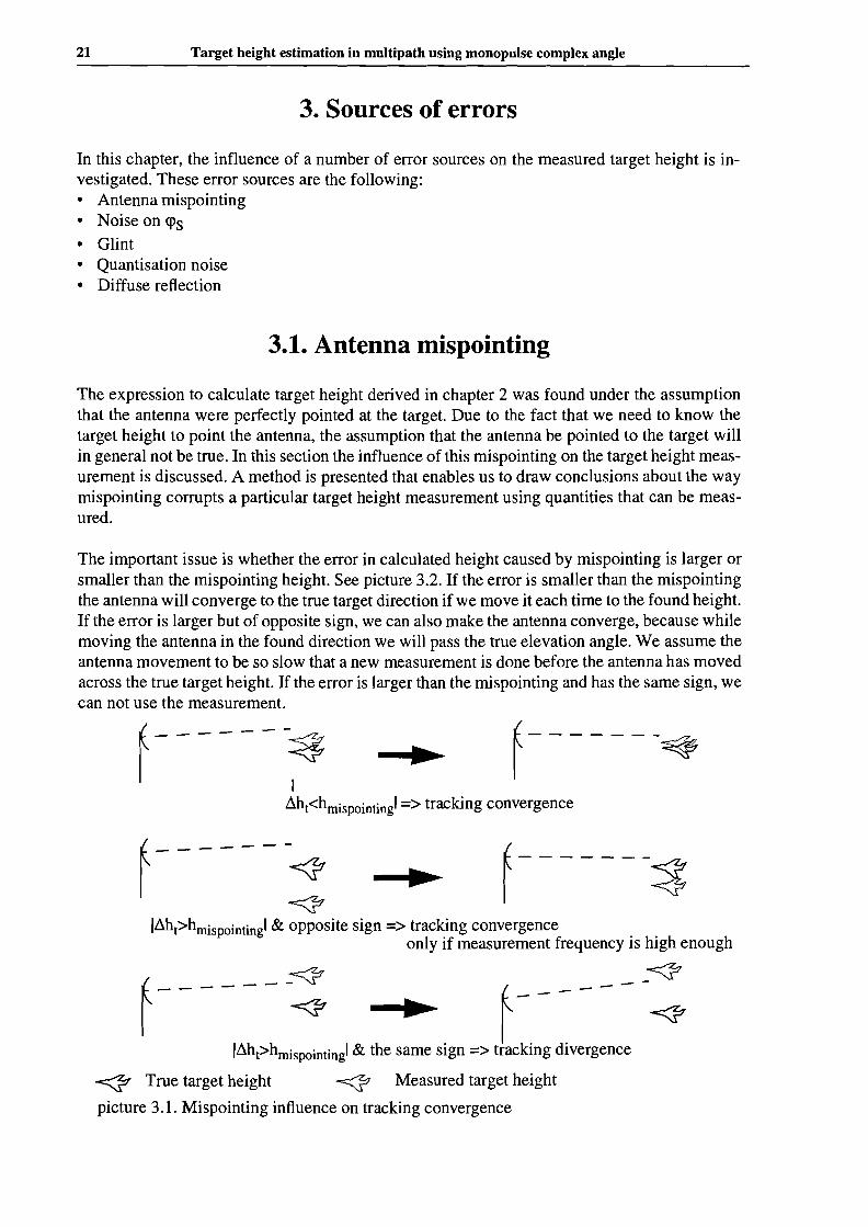
The important issue is whether the error in calculated height caused by mispointing is larger orsmaller than the mispointing height. See picture 3.2. If the error is smaller than the mispointingthe antenna will converge to the true target direction if we move it each time to the found height.If the error is larger but of opposite sign, we can also make the antenna converge, because whilemoving the antenna in the found direction we will pass the true elevation angle. We assume theantenna movement to be so slow that a new measurement is done before the antenna has movedacross the true target height. If the error is larger than the mispointing and has the same sign, wecan not use the measurement.f-------$
I
f- - - - - --~
Mlt<hmispointing' => tracking convergence
~-------
I -<}~
f-------:$IMlt>hmispointingl & opposite sign => tracking convergence
only if measurement frequency is high enough
~ _-<J7f- ------~ -l&t>hm~po;nHngl & ::::-s;gn => 1Cking diverg~ce <J"
~ True target height ~ Measured target height
picture 3.1. Mispointing influence on tracking convergence
Chapter 3. Sources of errors 22
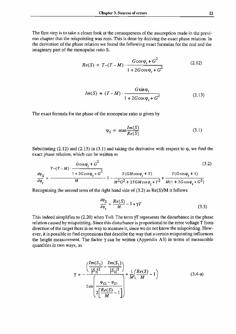
The first step is to take a closer look at the consequences of the assumption made in the previous chapter that the mispointing was zero. This is done by deriving the exact phase relation. Inthe derivation of the phase relation we found the following exact formulas for the real and theimaginary part of the monopulse ratio S.
Re(S)
2Gcos<i't + G=T-(T -M)· 2
1+ 2Gcos<i't + G
(2.12)
Im(S)Gsin<i't=(T-M)·----
21+ 2Gcos<i't + G
(2.13)
The exact formula for the phase of the monopulse ratio is given by
Im(S)<i's = atan Re(S) (3.1)
Substituting (2.12) and (2.13) in (3.1) and taking the derivative with respect to <i't we find theexact phase relation, which can be written as
2Gcosept + G (3.2)
T-(T-M)· 2depS 1 + 2Gcosept + G T(GMcosept + T) T(Gcosept + 1)
1 - + ------____::_dept - M M2G2 +2TGMcosept+T2 M(1+2Gcosept+G2)
Recognising the second term of the right hand side of (3.2) as Re(S)/M it follows
(3.3)
This indeed simplifies to (2.20) when T=O. The term if represents the disturbance in the phaserelation caused by mispointing. Since this disturbance is proportional to the error voltage T fromdirection of the target there is no way to measure it, since we do not know the mispointing. However, it is possible to find expressions that describe the way that a certain mispointing influencesthe height measurement. The factor y can be written (Appendix A3) in terms of measurablequantities in two ways, as
(3.4-a)
23 Target height estimation in multipath using monopulse complex angle
and as
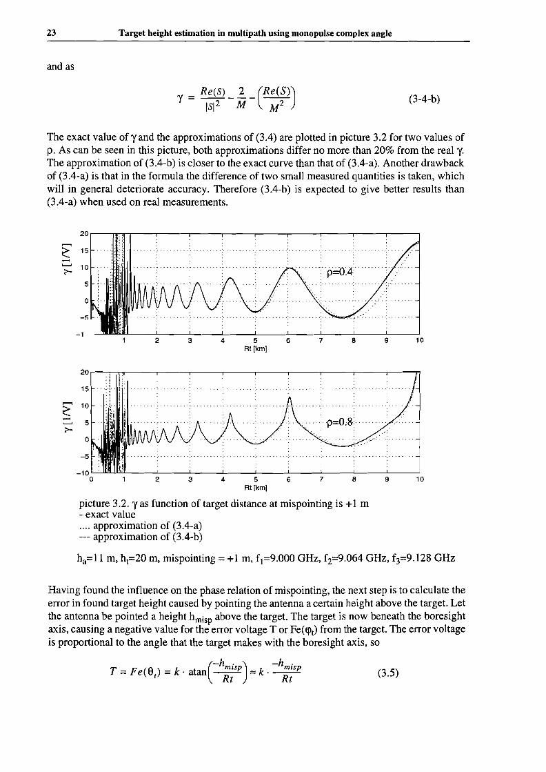
(3-4-b)
The exact value of y and the approximations of (3.4) are plotted in picture 3.2 for two values ofp. As can be seen in this picture, both approximations differ no more than 20% from the real y.The approximation of (3.4-b) is closer to the exact curve than that of (3.4-a). Another drawbackof (3.4-a) is that in the formula the difference of two small measured quantities is taken, whichwill in general deteriorate accuracy. Therefore (3.4-b) is expected to give better results than(3.4-a) when used on real measurements.
10987
·:.·········p·~OA····
65Rt [km]
432
", t.
". ".. ~; ~:.5
o
-1>
-1
~ 15 .....::ii ... /:!.....
.......... 10?-
20,----r....,......, --r----r----r---,------,----r----y------,.------,-----,"
20 ,----.----rT---,-----r---,.------,----,----r--r--,------,---T1
1098
.... - .
p=O$······
76432 5Rt[km]
picture 3.2. yas function of target distance at mispointing is +1 m- exact value.... approximation of (3.4-a)--- approximation of (3.4-b)
15
~ 10............... 5?-
ha=11 m, ht=20 m, mispointing = +1 m, f1=9.000 GHz, f2=9.064 GHz, f3=9.128 GHz
Having found the influence on the phase relation of mispointing, the next step is to calculate theerror in found target height caused by pointing the antenna a certain height above the target. Letthe antenna be pointed a height hmisp above the target. The target is now beneath the boresightaxis, causing a negative value for the error voltage T or Fe(q>t) from the target. The error voltageis proportional to the angle that the target makes with the boresight axis, so
T F (8) k (-hmisP) k -hmisp= e = 'atan--:::::: ._-
t Rt Rt (3.5)
Chapter 3. Sources of errors 24
in which k is the error voltage per unit of angle, a parameter of the monopulse system. In appendix A3 is derived that the error in the measured target height equals
(3.6)
(3.7)
In this expression htm is the target height with respect to the plane of reflection. Substituting(3.5) in (3.6) gives the relation between the mispointing height and the error in the measuredtarget height.
!1h t = htm . ykhmisp Rt 1 _ Re(S)
M
From equation (3.7) the condition under which mispointing will lead to a diverging error in thefound target height can be found. This is
htm . yk > 1Rt 1- Re(S)
M
(3.8)
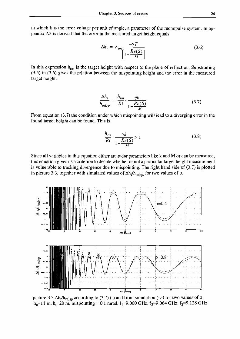
Since all variables in this equation either are radar parameters like k and M or can be measured,this equation gives us a criterion to decide whether or not a particular target height measurementis vulnerable to tracking divergence due to mispointing. The right hand side of (3.7) is plottedin picture 3.3, together with simulated values of I1ht/hmisp, for two values of p.
'"
Q.,enOs 0.5
.:; 0
..c-<l -0.5
_"1.5
'"
..
..
6At [klT'l
5At [krn]
..
..
"7
p=0.8'
"7
..
..
..
..picture 3.3l1ht/hmisp according to (3.7) (-) and from simulation (-.-) for two values of pha=ll m, ht=20 m, mispointing = 0.1 rnrad, f1=9.000 GHz, f2=9.064 GHz, f3=9.128 GHz
25 Target height estimation in multipath using monopulse complex angle
As can be seen from picture 3.3, equation (3.7) predicts the mispointing error quite well. However, in the peaks, differences occur. Especially at p=O.8, the rnispointing error has peaks while(3.7) has small dips superponed on the peaks that keep it below 1. These peaks and dips are dueto the error that is made by integrating only the three measured values of Re(S) instead of integrating all values of Re(S) between Al and 1..3, So for high values of p the threshold value of thecriterion beneath which we can use a height estimate should be taken much lower than one, orthe criterion should be combined with some other way of peak detection.
3.2. Noise on phase S
The measured phase <Ps of the monopulse ratio will in general have an error. Sources of this canbe for example
• noise• wavelength dependent phase differences between /). and L channel in the receiver• Quantisation noise on /). and L channel• glint• diffuse reflection
For measuring the target height we are interested in the difference of <Ps at two wavelengths. Apart of the error will be correlated and may cancel out when taking the difference, while a partwill be uncorrelated.
From the target height formula (2. 27) we learn that a certain phase difference error causes atarget height error according to
/).h t /).( /).<Ps)= (3.9)
ht /).<PsSo the relative error in target height is equal to the relative error in phase difference measurement. To obtain a small target height error, the phase difference should be taken as large as possible. At the same time it should be kept between -7t and +7t, to avoid ambiguity. Since the phasedifference /).<Ps is proportional to the radar frequency difference, the way to do this is to choosea suitable frequency difference.
A simulation is done with a normal distributed noise with a variance of 0.1 rad added to /).<Ps. Inpicture 3.4. the resulting target height and /).<Ps are plotted against range. It appears that when/).<Ps is small the error on ht is large. In this simulation /).f was 128 Mhz.

Chapter 3. Sources of errors
60,-----.-----.-----.-----.----,.-.---------,
50 .
26
20
10
~1~~~········li~,:·,:,'~~·.lhLJli;ii........r~~~'"~.
(3.10)
oOL...L.'---'-'----'---L----2L----
3L-----'-4L-------'-SL.l..---'----'---.J
6R[km]
4,----,-----,-----,-----,-----,---------,
3
2
~1
-30L--------JL--------J2L-------:3L--------J4L----SL-------:6
R[km]
picture 3.4. Effect of noisy L\CPs on the found target heightha=11 m, ht=20 m, mispointing = 0, f1,2,3= 9 GHz + -8, 0,8 * 8 MHz
To get an impression on the possibilities of reducing the error by choice of the frequency difference, a simulation has been done with the following choice of frequency difference.
L\f = 2· 1~8MHZ /\ /).f ~ 512MHzCPs
In which L\CPs was the mean of the measured /).CPs of four noisy simulations with L\f =12 MHz.In picture 3.5 the simulated target height measurement is plotted against range, as well as /).CPsand /)'f. In this picture it can be seen that for near ranges /).CPs is nearly constant 2 rad. For longerranges the wavelength difference gets to its maximal value. Here /).CPs is smaller and the targetheight is noisier. In general the noise on the target height is much smaller than in picture 3.4.However, using the full frequency interval to lower the influence of noise on L\cps, we do nolonger have the possibility to use frequency agility for other purposes.
27 Target height estimation in multipath using monopulse complex angle
30,------r----....---------r------.--------,------,
6543R[km]
2O...........LL.LL..-----'----_-'---- ----L ...L- ----'- --'
o
~20
.s:c
10
4,------r----....---------r------.--------,r-------,
'C 2~1Il 0:Ea."C -2
6543R[km]
2-4 '-----------'------'----------'-------'--------'------'
o40,-----,-----.---------r----...,-------,------,
o
N 20J:~
<0~
~ -20
-40 '----- ----'- -'-- ----'- --'-- ----1 ---'
o 234 5 6R[km]
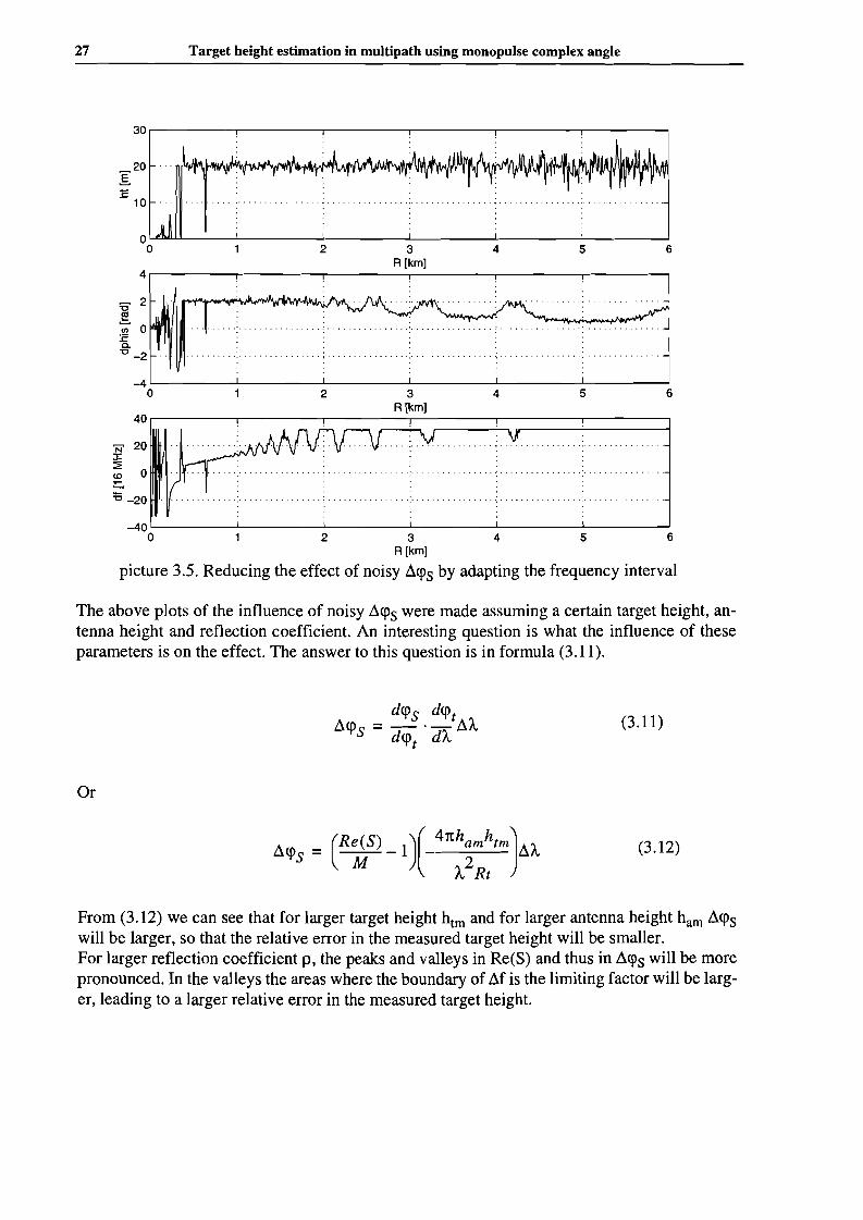
picture 3.5. Reducing the effect of noisy ~q>s by adapting the frequency interval
The above plots of the influence of noisy ~q>s were made assuming a certain target height, antenna height and reflection coefficient. An interesting question is what the influence of theseparameters is on the effect. The answer to this question is in formula (3.11).
(3.11)
Or
(3.12)
From (3.12) we can see that for larger target height htm and for larger antenna height ham dq>Swill be larger, so that the relative error in the measured target height will be smaller.For larger reflection coefficient p, the peaks and valleys in Re(S) and thus in dq>s will be morepronounced. In the valleys the areas where the boundary of ~f is the limiting factor will be larger, leading to a larger relative error in the measured target height.

Chapter 3. Sources of errors
3.3. Glint
28
Measuring the position of a target is based on the assumption that the electromagnetic wavesreflected by the target proceed from the geometric centre of the target. For targets smaller thanthe wavelength this is true. For larger targets however the electromagnetic point of gravity maybe shifted in all coordinates, distance, azimuth, elevation and doppler frequency. This phenomenon is called glint. The position of the electromagnetic point of gravity depends of the relativephase and strength of the electromagnetic waves reflected at the different parts of the target surface. Due to changes in the target orientation and to mechanical oscillations amongst differentparts of the target the position of the electromagnetic point of gravity varies in a stochastic way.
According to [Nooy] the glint distribution can be well approximated with a normal distribution.For uniform distributed scatterers over the span L of the target the position of the electromagnetic point of gravity along the span direction has a standard deviation of:
(3.13)
For most aeroplanes O'gl is between L/4 and L/6.
The way glint errors cause an error in the target height as measured according to (2.27) may beunderstood from the following:
Glint causes random shifts in the apparent target height and the apparent target range that differeach measurement. These shifts cause a random shift in the phase difference between the directand indirect path according to
So the standard deviation on <Pt is
41thamO'htm 41thamO'RtO'<Pt = ARt + AR 2
t
This causes an error on the phase of the monopulse ratio
(2.10)
(3.14)
(3.15)
Because this error is assumed to be uncorrelated between two measurements, the standard deviation of the error in the phase difference ~<Ps between two measurements will be
(3.16)
29 Target height estimation in multipath using monopulse complex angle
The standard deviation of the relative error in target height follows from (3.9)
(3.17)
To get insight in the order of magnitude of the error, let us fill in some values:
Assume the target height to be 20 m, the antenna height to be 10 meter, the wavelength to be0.03 m and the range to be 2000 m. According to 3.14 the error on the phase between direct andindirect path is
(3.18)
From which we can conclude that the influence of target height glint is much more importantthan that of target range glint.
Assume the target to be an F-16. This aeroplane has a length of 15 m and a height of 5 m. Sothe standard deviation of the target range glint aRt will be 5 m and the standard deviation of thetarget height glint aht will be approximately 1 m. Filling in these values in (3.18) gives
a<j)t = 2.1 . 1 + 0.0010 ·5 = 2[rad] (3.19)
(3.20)
As can be seen in picture 3.4 the phase difference L1<j)s will be at maximal about 2 rad. Thereforewe can expect a severe error: the standard deviation of the error is larger than L1<j)s itself. Furthermore, the error will fold itself back around plus and minus 1t, giving a distorted signal thatis hard to filter. The error on target height will therefore be not normal distributed and as largeas the maximal measurable target height.
Assume the target to be an Exocet missile. This missile has a length of 5 m and a diameter of0.35 m. The standard deviation of the target range glint aRt will be 2 m and the standard deviation of the target height glint aht will be approximately 0.1 m. Filling in these values in (3.18)gives
a<j)t = 2.1 ·0.1 + 0.0010 . 2 = 0.21 [rad] (3.21)
(3.22)
The phase difference L1<j)s is about 2 rad. So according to (3.17) the error on the measured targetheight will be normal distributed with a standard deviation of 15% of the target height.

Chapter 3. Sources of errors 30
3.4. Quantisation noise
In the monopulse receiver the sum and delta signals are AID converted. This will cause quantisation noise. In this chapter is investigated how large this noise is and how it corrupts the phasemeasurement. Because the way the digital signals are processed in the Multiple Target TrackingUnit (MTTU) will eliminate a large part of the errors, this step is taken into account as well.
L e(~) Re(~)
m(~)32 pts
Im(~)
e(Llli f/3 e(Llli)~E AGC Modulator
m(Llli FFf Im(Llli)
~Ae(M e(M)
m(M m(M)
IF 15 MHz I 5 MHz Frequency domainAGC gain Phase ref. I
Receiver I MTTU
picture 3.6 AID conversion and Doppler processing of the Sum and Delta channels
In picture 3.6. a part of the receiver and of the MTTU is drawn. At the left side the sum and deltachannels, having been modulated from radio frequency into intermediate frequency before,come into the automatic gain control (AGC). The AGC is adjusted in steps of 3 dB so that themean value of the AID converted sum signal is 48. The delta channels are amplified with thesame AGC factor. In the modulator, the signals are modulated with a reference signal to obtainthe in-phase and quadrature components. These are AID converted at a sample frequency of 15MHz and fed into the MTTU.
At this point we have the real and imaginary part of the sum signal and of the delta signals. Thesum signal has a mean value of 48 and will typically lying between 32 and 64, although largervalues may occur. The delta signals will in general be much smaller than the sum signal. Therefore, relatively large quantisation errors may occur in the delta signals.
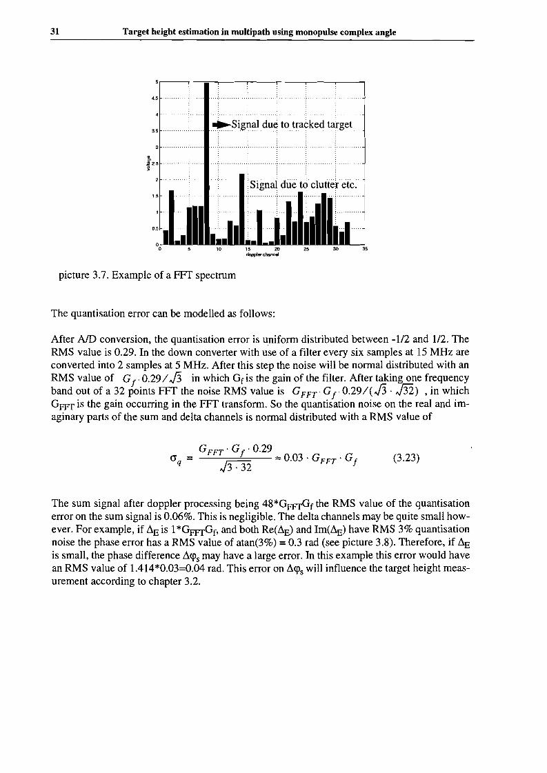
In the MTTU the incoming signals are first down converted to a sample frequency of 5 MHz.Then a 32 points Fast Fourrier Transform (FFT) is done. After this step, the signals are in thefrequency domain. Because of the doppler effect, the frequency band in which a signal originating from a certain radiation source comes, depends on the velocity of this source towards theradar antenna. So after the FFf signals originating from sources other than the target, like bullets fired from our ship to the target and sea clutter, will be in other frequency bands than thesignals we get directly and via the sea surface from the target. The latter is the case because thevirtual target travels at the same speed as the real. Only the frequency band in which the signalsfrom the target are is taken to give the final values of the sum and delta channels. In the case ofpicture 3.7. for example the signal of doppler channel 8 would be taken, thus getting rid of allnoise present in other doppler channels.
31 Target height estimation in muItipath using monopulse complex angle
4.5 .
4 .
3.5 .
8..l! 2.5 .~
2 ...
1.5
Signal due to clutte'retc~
35
picture 3.7. Example of a FFT spectrum
The quantisation error can be modelled as follows:
After AID conversion, the quantisation error is uniform distributed between -1/2 and 1/2. TheRMS value is 0.29. In the down converter with use of a filter every six samples at 15 MHz areconverted into 2 samples at 5 MHz. After this step the noise will be normal distributed with anRMS value of Gf' 0.29/J3 in which Gf is the gain of the filter. After taking one frequencyband out of a 32 points FFT the noise RMS value is Gppr' Gj' 0.29/( J3 .J32) ,in whichGFF[ is the gain occurring in the FFT transform. So the quantisation noise on the real and imaginary parts of the sum and delta channels is normal distributed with a RMS value of
Gppr ' Gf · 0.29CJq = J3:n z 0.03 . Gppr . Gf (3.23)
The sum signal after doppler processing being 48*GFF[Gf the RMS value of the quantisationerror on the sum signal is 0.06%. This is negligible. The delta channels may be quite small however. For example, if ~E is 1*GFF[Gf , and both Re(~E) and Im(~E) have RMS 3% quantisationnoise the phase error has a RMS value of atan(3%) = 0.3 rad (see picture 3.8). Therefore, if ~Eis small, the phase difference ~<j>s may have a large error. In this example this error would havean RMS value of 1.414*0.03=0.04 rad. This error on ~<j>s will influence the target height measurement according to chapter 3.2.

Chapter 3. Sources of errors 32
1m
RMS=0.03______-+-====:=-- --\-....;:;-__-.+ Re
11
picture 3.8. Example error £ in phase ~E signal
A simulation has been done with quantisation noise added to the real and imaginary parts of sumand difference signals. The quantisation noise was modelled as white gaussian noise with aRMS value of 0.03. The filter and FFT have not been included in detail in the simulation, because we are only interested in the noise reduction they cause, which is already accounted forin the RMS value 0.03. Consequently, GFFf and Gf are taken 1. The simulation results are inpicture 3.9. The noise on ~<Ps is largest between the peaks, because there L is large compared to~E' Since quantisation noise is basically noise on ~<Ps the resulting error on target height is according to the analysis of chapter 3.2. A possible way of reducing the error is the same as inchapter 3.2: choosing the transmitter frequencies further apart.
9 10
9 10
87456R[km]
32
00 2 3 4 5 6 7 8 9 10
1
.....
picture 3.9. Simulated effect of quantisation noise
33 Target height estimation in multipath using monopulse complex angle
3.5 Diffuse reflection
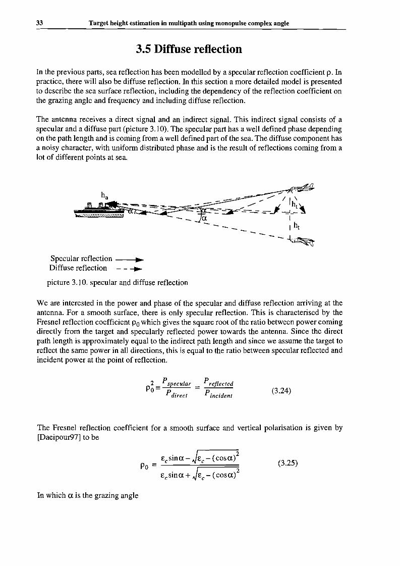
In the previous parts, sea reflection has been modelled by a specular reflection coefficient p. Inpractice, there will also be diffuse reflection. In this section a more detailed model is presentedto describe the sea surface reflection, including the dependency of the reflection coefficient onthe grazing angle and frequency and including diffuse reflection.
The antenna receives a direct signal and an indirect signal. This indirect signal consists of aspecular and a diffuse part (picture 3.10). The specular part has a well defined phase dependingon the path length and is coming from a well defined part of the sea. The diffuse component hasa noisy character, with uniform distributed phase and is the result of reflections coming from alot of different points at sea.
--~
Specular reflection --..~~Diffuse reflection - - ...
picture 3.10. specular and diffuse reflection
We are interested in the power and phase of the specular and diffuse reflection arriving at theantenna. For a smooth surface, there is only specular reflection. This is characterised by theFresnel reflection coefficient Po which gives the square root of the ratio between power corningdirectly from the target and specularly reflected power towards the antenna. Since the directpath length is approximately equal to the indirect path length and since we assume the target toreflect the same power in all directions, this is equal to the ratio between specular reflected andincident power at the point of reflection.
2 _ Pspecular _ PreflectedPO= - -.::..;..;",,;~
Pdirect Pincident(3.24)
The Fresnel reflection coefficient for a smooth surface and vertical polarisation is given by[Daeipour97] to be
In which a is the grazing angle
Po =Ecsina - JEc - (cosa)2
Ecsina + JEc - (cosa)2
(3.25)
Chapter 3. Sources of errors
and Ec the complex dielectric constant, given by
(3.26)
34
In which E is the dielectric constant of the reflecting surface, 0' its conductivity and Athe wavelength of the reflected electromagnetic wave.
In the case of sea water Ec is
Ec = 81-278j· A
In the case of a rough surface, specular ret1ection is reduced and diffuse reflection occurs. Specular reflection is reduced by the specular scattering factor Ps according to:
pC1Pol. P
s)2 == specular
Pdirect
This specular scattering factor is given by [Beckmann 63] to be
( (21t0'h sin U)2)
Ps = exp -2· A
In which O'h is the RMS waveheight and", is the grazing angle
(3.27)
(3.28)
The diffuse ret1ection coefficient Pd gives the relation between the power reflected directly fromthe target and the power reflected diffuse from the sea towards the antenna. It is defined by
(3.29)
The value of Pd is difficult to calculate, since reflected power should be integrated over a largereflecting surface. This integration is treated in [Beckmann 63], [de Vries88] and [Barton74].To enable quick Matlab simulations we will use a more simple model, using values for the diffuse reflection coefficient from literature [Barton74], [Daeipour97]. We will assume the diffusereflection to be proceeding from one point at sea.
35 Target height estimation in multipath using monopulse complex angle
The received monopulse ratio is modelled as:
The first terms represent the signal coming directly from the target.
The second terms represent the specular reflection. It is characterised by the Fresnel reflectioncoefficient Po and the roughness factor Ps which accounts for the decrease of the reflected signalstrength.
The third terms represent diffuse reflection. Diffuse reflection is assumed to be coming fromone point and to have a normal distributed strength with a RMS value of POPd' The diffuse reflection coefficient Pd is described in literature [Barton74]. According to a more detailed model[de Vries], the amount of diffuse power entering the antenna also depends on the antenna gainin the direction of the sea. We will apply the value of Pd given by Barton and make a rough correction for the small beamwidth of the STING-EO.
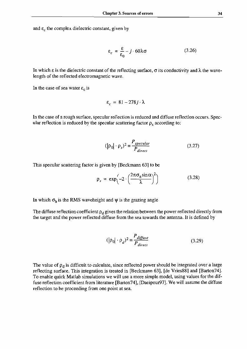
The relation between reflection coefficients and surface roughness as given by [Beckmann63]and [Barton74] is plotted in picture 3.11.
.....0.9s:::
Q).- psu8 0.8
Q)0U 0.7s:::.S..... 0.6U
Q)
4::Q) 0.5'-<Q)CI:l
c.2 0.4.......:a"'lj 0.3
s:::~
'-< 0.2~-;::lU
0.1Q)
0..C/)
OL.....<::::::..-...L-_....l-_---L_---L_----..Jl.-_.l....-_...L-_--..l-_--L_---'o 0.02 0.04 0.06 0.08 0.1 0.12 0.14 0.16 0.18 0.2
Roughness =
picture 3.11 Specular and diffuse reflection coefficients versus roughness
Chapter 3. Sources of errors
From this picture, Pd can be approximated as
( ( (3.51tCfhSina)2))Pd::::: 0.4· 1 - exp -2· A (3.31)
36
In the simulation, diffuse reflection is modelled as noise with a gaussian distribution in amplitude and a uniform distributed phase. From measurements [L090],[L091] is known that diffusereflection has a decorrelation time in the order of a second. This is taken into account in the simulation model by applying a n-points moving average filter, with n the number of samples persecond. To keep the power equal, the signal is multiplied with JO .The diffuse reflection is assumed to come from the specular reflection point.
Picture 3.11 is obtained assuming a wide antenna beam. It has been confirmed by measurements[Beard 61] with antennas with a beam width of 20° and 8°. The STING-EO has a beam widthof approximately 1.4°. Therefore the diffuse reflection perceived by the antenna will be smaller.To take this into account the diffuse signal has been attenuated by a factor two. This value isbased on the observation that diffuse reflection is often concentrated in a foreground and a horizon component. Due to the small antenna beam, the foreground component will not be perceived. Assuming the horizon component to contain approximately half the power, the factortwo is found. Still, not taking into account the pointing direction of the antenna, mistakes maybe made.
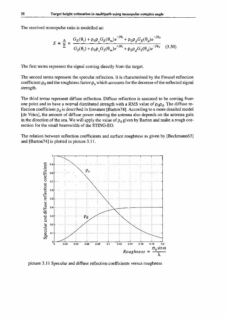
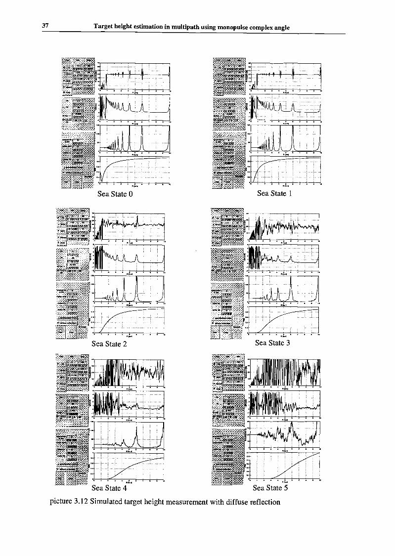
In picture 3.12 simulation results are given at various sea states. In this picture, it is visible howdiffuse reflection disturbs ~q>s in a growing way, as the sea state gets larger. In all pictures canbe seen how when Ps decreases the noise on ~q>s gets larger, until ~q>s starts folding back. In thelatter case the found target height is nonsense. Before this point, the found target height is noisy,but the mean corresponds to the true target height.
Although hard quantitative conclusions can not be drawn from this simple model, some qualitative reasoning about the influence of different parameters may be done:
Larger ~q>s: since diffuse reflection basically causes noise in ~q>s larger ~q>s will reduce target,height errors (see section 3.2). However, folding back will occur at approximately the samepoint.
Target distance: as can be seen in the picture, larger target distance gives better measurements.
Target height or antenna height: larger target or target height gives a larger grazing angle, thusmore diffuse reflection. On the other hand it increases ~q>s. The over all effect will be similar tothat of increasing 11Rt• Thus larger target or antenna height causes a larger target height measurement error.
37 Target height estimation in multipath using monopulse complex angle
~ :' I.' .~ : . .1.
!M,'J-. ., ,-40 , 2 3 .... 7 •• 10
:~ .., .. ]J~'!'lo.a ,•..•.......... - ; .
DO , r , • • • '0......Sea State 0
]~
lkfl"j.....Sea State 2
~,' ' ." . - -'!'.10 ... , ... ,.... : .... _,'. :
. . ..
_E#1DIGJJ ±i
: : : ~ .
'. ; }. :' i 3 :
~1......Sea State 4
lUlU]; ..J:~I· ••••·~.'j..:.. f·-.·.·. i..'· .11.._ALIi.: _
DO 1 r 3 of ~. "0......Sea State 1
~~.".... :. :._.•.• :.•. ~f:..•. :..••.j.•.'.s .;..,. ." , , , , .
II .; ....;. ., - , ._ ,.•
, _. . ,.. , ", "; , .
_: . .II ..•••.••...........•. '. ~ .••... '_'..
ttllEl')l:~
Sea State 3
Sea State 5
picture 3.12 Simulated target height measurement with diffuse reflection
Chapter 4. Phase calibration of the STING-EO 38
4 Phase calibration of the STING-EO
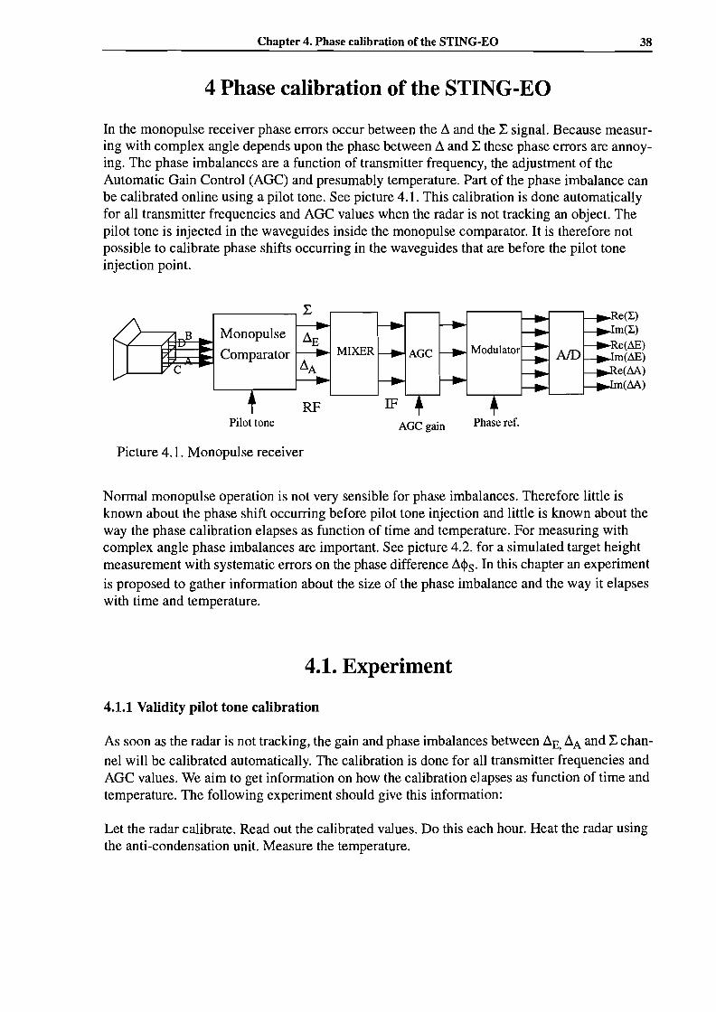
In the monopulse receiver phase errors occur between the ~ and the L signal. Because measuring with complex angle depends upon the phase between ~ and L these phase errors are annoying. The phase imbalances are a function of transmitter frequency, the adjustment of theAutomatic Gain Control (AGC) and presumably temperature. Part of the phase imbalance canbe calibrated online using a pilot tone. See picture 4.1. This calibration is done automaticallyfor all transmitter frequencies and AGC values when the radar is not tracking an object. Thepilot tone is injected in the waveguides inside the monopulse comparator. It is therefore notpossible to calibrate phase shifts occurring in the waveguides that are before the pilot toneinjection point.
Phase ref.
Modulator
AGe gain
MIXER
Pilot toneRF
B Monopulse'f---a~=c~ Comparator
Picture 4.1. Monopulse receiver
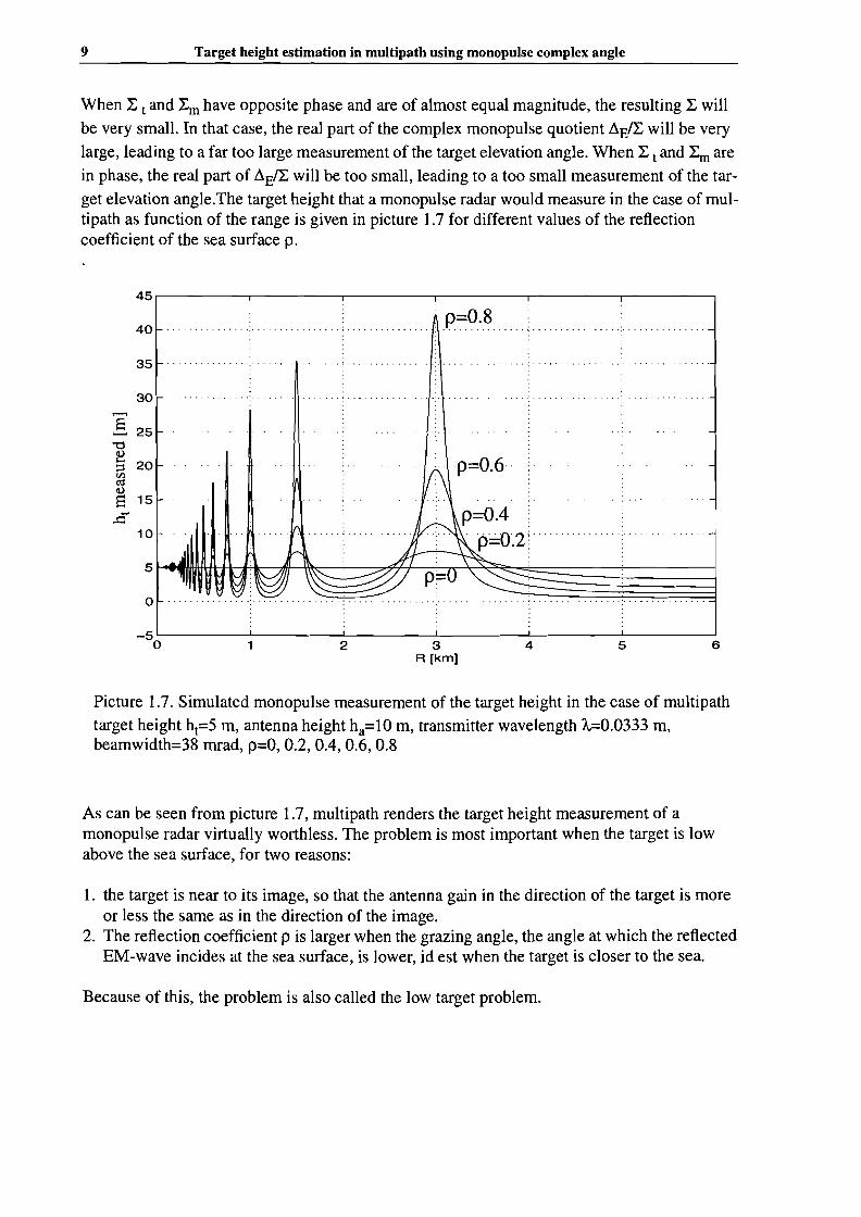
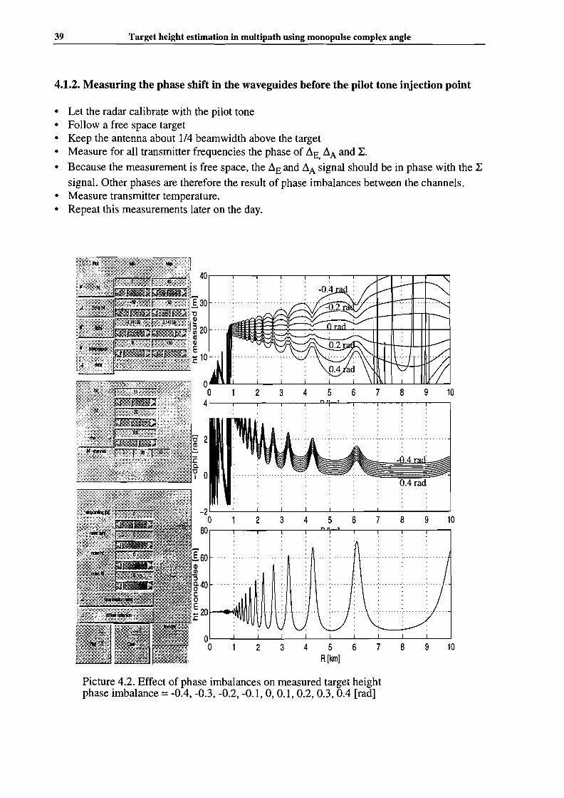
Normal monopulse operation is not very sensible for phase imbalances. Therefore little isknown about the phase shift occurring before pilot tone injection and little is known about theway the phase calibration elapses as function of time and temperature. For measuring withcomplex angle phase imbalances are important. See picture 4.2. for a simulated target heightmeasurement with systematic errors on the phase difference ~<l>s. In this chapter an experimentis proposed to gather information about the size of the phase imbalance and the way it elapseswith time and temperature.
4.1. Experiment
4.1.1 Validity pilot tone calibration
As soon as the radar is not tracking, the gain and phase imbalances between ~E, ~A and L channel will be calibrated automatically. The calibration is done for all transmitter frequencies andAGC values. We aim to get information on how the calibration elapses as function of time andtemperature. The following experiment should give this information:
Let the radar calibrate. Read out the calibrated values. Do this each hour. Heat the radar usingthe anti-condensation unit. Measure the temperature.
39 Target height estimation in multipath using monopulse complex angle
4.1.2. Measuring the phase shift in the waveguides before the pilot tone injection point
• Let the radar calibrate with the pilot tone• Follow a free space target• Keep the antenna about 1/4 beamwidth above the target• Measure for all transmitter frequencies the phase of ~E ~A and L.,• Because the measurement is free space, the ~E and ~A signal should be in phase with the L
signal. Other phases are therefore the result of phase imbalances between the channels.• Measure transmitter temperature.• Repeat this measurements later on the day.
-20 2 3 4 5 6 7 8 9 10
80
I60 . . . . . . ... . . ........ ......CD!!1:J§-40 • • • • • • l • • • • • • .• 1. ..........c:0
: 20~
00 2 3 4 5 6 7 8 9 10
R[km]
Picture 4.2. Effect of phase imbalances on measured target heightphase imbalance =-0.4, -0.3, -0.2, -0.1, 0, 0.1, 0.2, 0.3, 0.4 [rad]
Chapter 5. Target height measurements from real data
5. Target height nleasurements from real data
40
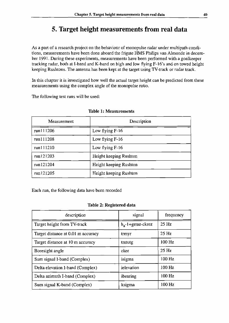
As a part of a research project on the behaviour of monopulse radar under multipath conditions, measurements have been done aboard the frigate HMS Philips van Almonde in december 1991. During these experiments, measurements have been performed with a goalkeepertracking radar, both at I-band and K-band on high and low flying F-16's and on towed heightkeeping Rushtons. The antenna has been kept at the target using TV-track or radar track.
In this chapter it is investigated how well the actual target height can be predicted from thesemeasurements using the complex angle of the monopulse ratio.
The following test runs will be used:
Table 1: Measurements
Measurement Description
run111206 Low flying F-16
run111208 Low flying F-16
run111210 Low flying F-16
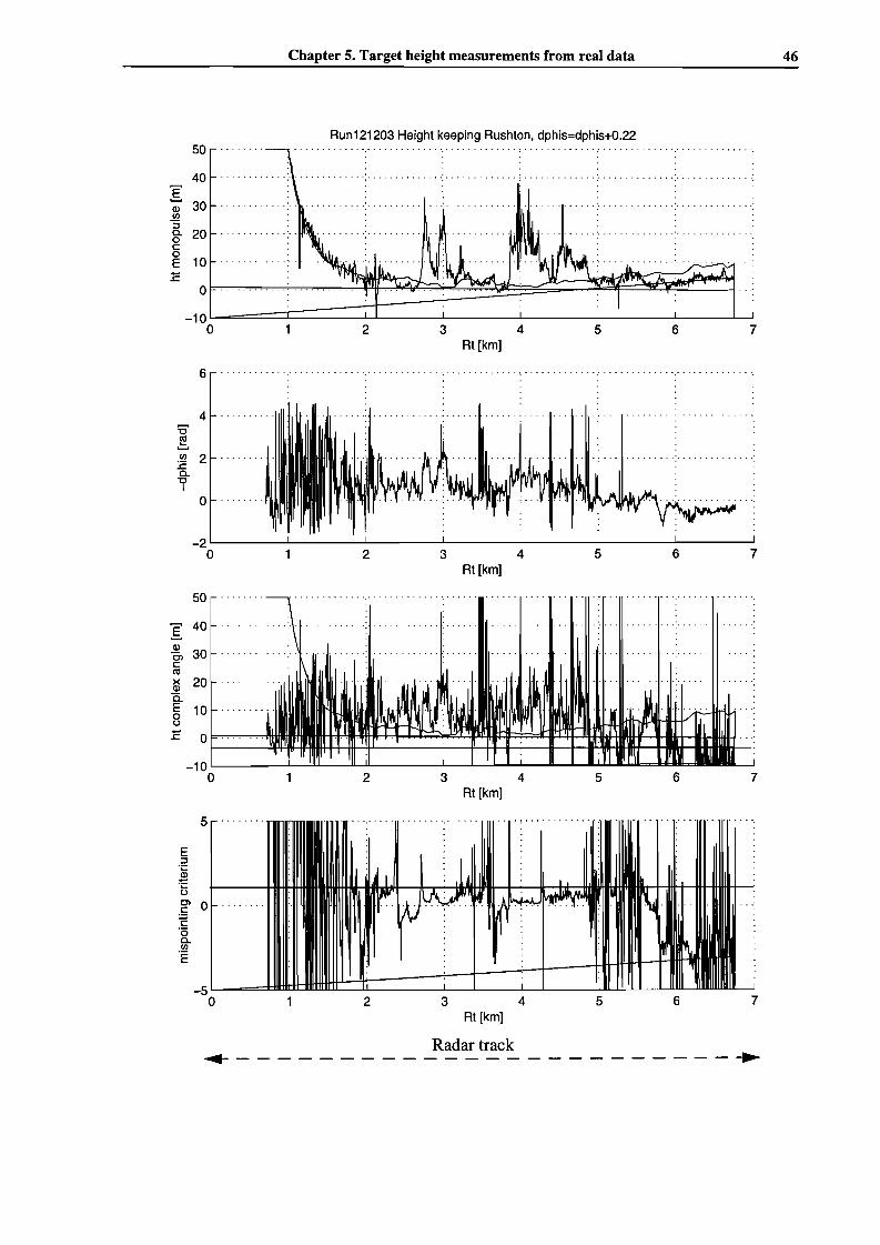
run121203 Height keeping Rushton
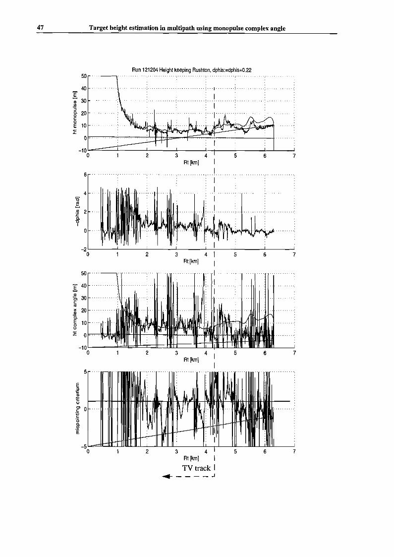
run121204 Height keeping Rushton
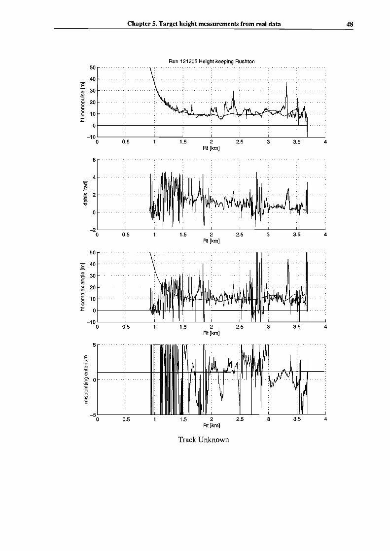
run121205 Height keeping Rushton
Each run, the following data have been recorded
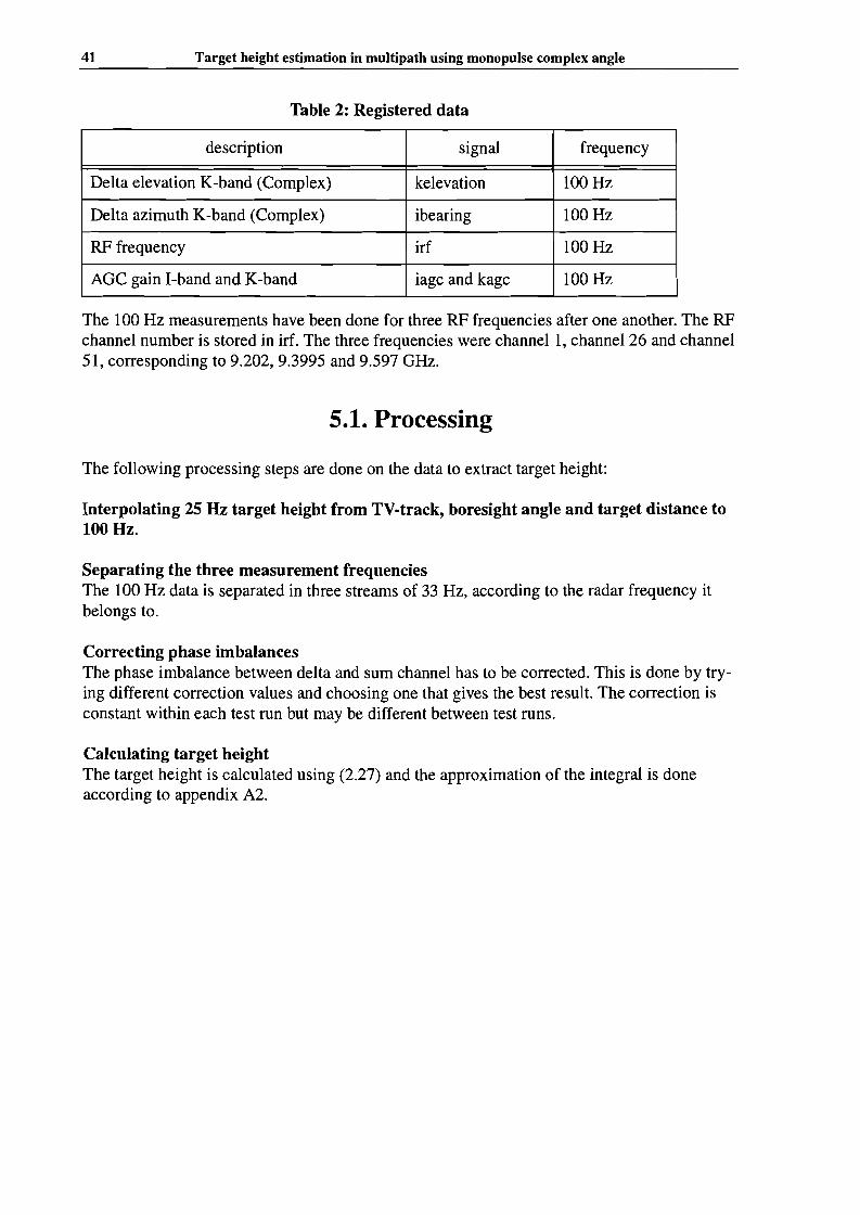
Table 2: Registered data
description signal frequency
Target height from TV-track ha-l+grmz-ckrez 25Hz
Target distance at 0.01 m accuracy trmyr 25Hz
Target distance at 10m accuracy tmtutg 100Hz
Boresight angle cker 25 Hz
Sum signal I-band (Complex) isigma 100Hz
Delta elevation I-band (Complex) ielevation 100Hz
Delta azimuth I-band (Complex) ibearing 100Hz
Sum signal K-band (Complex) ksigma 100Hz
41 Target height estimation in multipath using monopulse complex angle
Table 2: Registered data
description signal frequency
Delta elevation K-band (Complex) kelevation 100Hz
Delta azimuth K-band (Complex) ibearing 100Hz
RF frequency irf 100Hz
AGC gain I-band and K-band iagc and kagc 100Hz
The 100 Hz measurements have been done for three RF frequencies after one another. The RFchannel number is stored in irf. The three frequencies were channel 1, channel 26 and channel51, corresponding to 9.202,9.3995 and 9.597 GHz.
5.1. Processing
The following processing steps are done on the data to extract target height:
Interpolating 25 Hz target height from TV-track, boresight angle and target distance to100 Hz.
Separating the three measurement frequenciesThe 100 Hz data is separated in three streams of 33 Hz, according to the radar frequency itbelongs to.
Correcting phase imbalancesThe phase imbalance between delta and sum channel has to be corrected. This is done by trying different correction values and choosing one that gives the best result. The correction isconstant within each test run but may be different between test runs.
Calculating target heightThe target height is calculated using (2.27) and the approximation of the integral is doneaccording to appendix A2.

Chapter 5. Target height measurements from real data
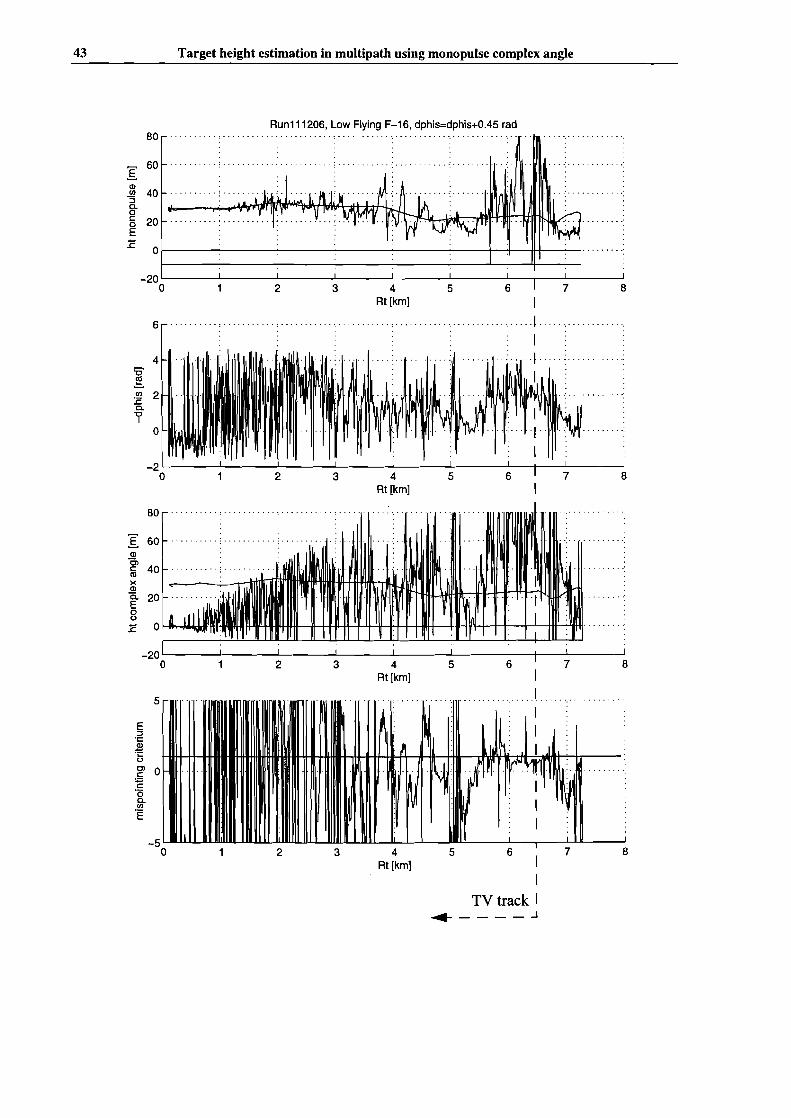
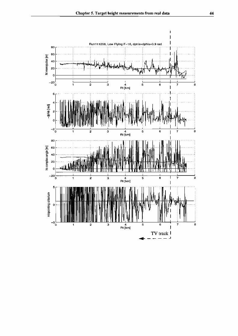
5.2. Results
For all runs the following plots have been made:
1. Target height as measured with standard monopulse method2. Phase difference ~<Ps.
3. Target height calculated from complex angle4. Mispointing divergence criterion
Everything is in earth coordinates
Beneath the figures the distance at which TV track was started is indicated (Source[Setyowati92] and [Bongers92])
42
43 Target height estimation in multipath using monopulse complex angle
Run111206, Low Flying F-16, dphis=dphis+O.4S rad
8
8
8
7
7
7
6
6
5
5
4Rt[km]
4Rt [km]
4Rt[km]
3
3
3
2 3 4 5 6 7 8Rt [km] I
ITV track I
.... ____ J
2
2
2
-20 L-__---'- ....L ...L.- L-__---'- -'--_+-_..I..-__----'o
_S .........u..uULI.JIII
o
5
80
I60
CD
'" 40"3a.0c:: 200EE
0
-200
6
4'0~
'" 2Ea.
"CI
0
-20
80
I 60 .CDtillii 40xCD
Ci. 20EooE
Chapter S. Target height measurements from real data 44
Run111208, Low Flying F-16, dphis=dphis+0.9 rad
8
8
8
7
7
7
6
6
6
ITV track I
-----'
1
......... 1-I- .... r'
... 1.
5
5
5
4Rt[km]
4Rt[km]
4Rt[km]
3
3
2
2
2 3
o
4
6 .....
-2 L- .L- ...l...- ....L... ....L.. --'- --'-__..:....----I. ---'
o 234 5 6 7 8Rt[km]
80
:[ 60.l!!C>
40I:
'")(.l!!Q. 20E0<.>~ 0
-200
5
E::::lg"5C> 0I:
~'0Q.
.!!1E
-50
80
:[ 60
<1l40.!!J.
::::lQ.0I: 200E~ 0
-200
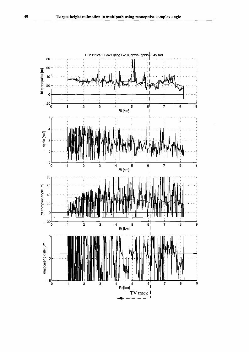
45 Target height estimation in multipath using monopulse complex angle
80
60I
CD-5 400o§ 20E
I... '.. ~un1.11210.' .Lo~ .FI~ing F~16: ~PhiS~dP~i~tO"~5 rad ..
: I...... .······r·..:J. .
~~~4'fIffl~~~~~~J1 :I
01-----------------+----1-----------.,
9
9
9
9
8
8
8
8
7
7
7
7
4 5Rt[km)
4 5Rt[km)
456Rt[km) I
TV track I~ .J
4 5Rt [km]
3
3
3
3
2
2
2
2
-2 '-------'---------L---'-------'--------'--------J'-t----'-----'------'o
-20 '---__....L-__---L '---__....L-__---L I.f-__--'----__---L__-----J
o
-20 1.-__...l.-__---L l-__...l-__---L 4--__...l-__---L__----'
o
_5L--o
E::J.;:
.2!";:og> 0E"00-f/)
"E
4
o
6
80 .
5
~11 20-0I
I 60CD0>1ij 40xCDa. 20E81: 0 I------i'
Chapter 5. Target height measurements from real data 46
Run121203 Height keeping Rushton, dphis=dphis+0.2250 ...
40E
30Q)Ul
""50- 200c:0E 10E
0
-100 2 3 4 5 6 7
Rt [km]
6 "," '," '"......... . "
4 ..... ... . . . . . . . . . ... .
'0~Ul 2:E0-"0
I
0
-20 2 3 4 5 6 7
Rt [km]
50
E 40
Q)
30Olc:ellX 20Q)
0..E 100(,)
E 0
-100 2 3 4 5 6 7
Rt [km]
5 ........
E::l';::
.s';::(,)
01 0C
~'00-Ul
'E
-50 2 3 4 5 6 7
Rt [km]
Radar track~- -- - - -- -- ---- - - - - - - - - ---~
47 Target height estimation in multipath using monopulse complex angle
Run 121204 Height keeping Rushton, dphis:=dphis+0.22
···· .... ·;···1·········:·····
50
40
I30Q)
m"S0- 200c:0E 10E
0
-100 2 3
Rt[km]4 5 6 7
6 '" .
4'0~m 2:c0-'0I
0 ..........
-20 2 3 4 5 6 7
Rt[km]
50
I 40Q)
30Olc:IIIX 20Q)
C.E 100(J
E 0
-100 2 3 4 5 6 7
Rt[km]
5
E:::I.~
~Cl 0 ...c:
:;:c:'00-m'E
-50 7
Rt[km] ITV track I
.... ____ ..1
Chapter 5. Target height measurements from real data
Run 121205 Height keeping Rushton
48
50 .
40
I(J) 30U>"3g- 20coE 10
Of---------------------------.1..-t-10 '--__---I. ---'- ...J- .l...-__----' ----'- --'-----'__
o 0.5 1.5 2 2.5 3 3.5 4Rt[km]
6 .
4
~:2 2c."0
I
o
-2 '--__---'- ---'- ...J- .l...-__----' ----'- --'-__----'
o 0.5 1.5 2 2.5 3 3.5 4Rt[km]
50
I 40
~ 30cCIl
~ 20C.E 1081: Ol-----------l
-1 0 L-__----' ----'-__.l...---'-_L..--'---'--__----J'----'-...........----'- ..........----J_~
o 0.5 1.5 2 2.5 3 3.5 4Rt[km]
0.5
5
-5 '--__----' JJJ.L-lll...
o 1.5 2Rt[km]
2.5 3 3.5 4
Track Unknown
49 Target height estimation in multipath using monopulse complex angle
5.3. Conclusions
As expected due to the high sea state (Sea State 4) not much low target effect occurs.
The F-16's give worse target height measurements with complex angle than the Rushtons. Tworeasons for this can be thought of:- higher glint- larger target height and consequently a larger grazing angle, causing less specular and morediffuse reflection.
Noise on ~<Ps grows at smaller distances. This is conform the results of the diffuse reflectionmodel.
On different plots, different ~<Ps corrections gave the best result. This would indicate that the
phase imbalance has changed between measurements. Because it was often difficult to seewhich was the best result, hard conclusions can not be drawn from this observation.
In the Rushton plots, outside the folding back area ~<Ps is not very noisy. However, within this
area there are small areas where large spikes occur.
In run121205 the mispointing criterion is consistent with itself, meaning that it does remainabove or below threshold for longer times. In run121204, runll1206 and runll1210 this isalso the case on many places though there are spiky areas. In runll1208 it is very noisy and inrun 121203 it does not behave as expected.
In run121205 and run121204 the non-spiky areas give the correct target height with an RMSerror of 5 m. Due to the high noise frequency, low pass filtering will improve the target heightmeasurement.
Chapter 6. Algorithm tuning
6. Algorithm tuning
50
In chapter 3 the influence of some error sources on the target height measurement was investigated. In this chapter it is described in more detail how the influence of error sources can beminimized by a good choice of measurement parameters. The choice of transmitter frequenciesis discussed in section 6.1. In section 6.2. is discussed how the antenna servo angular velocityshould be to prevent tracking divergence when the measured target elevation is beyond theactual target elevation.
6.1. Choice of transmitter frequencies
In many monopulse radars the transmitter frequency can be varied. In the STING the frequency can be varied around 9 GHz according to:
f = 9GHz + k . 8MHz
in which
kEN, -32 :5 k :5 32
In this section the choice of transmitter frequency is discussed and an algorithm to choose it isgiven.
The most serious limit on measuring target height is the effect of antenna rnispointing. If mispointing makes the tracking diverge, the measurement is useless, no matter how low the noiseis. So the first condition that has to be met is that rnispointing does not make the trackingdiverge. When this condition is met, we can start thinking about lowering the influence of othererror sources. Avoiding mispointing is investigated in section 6.1.1, while a way to reduce theother errors is discussed in section 6.1.2.
The outcome of the analysis of measurement errors in chapter 3 is that the choice of the frequency step influences the size of the phase step ~<Ps and by that means influences the signal to
noise ratio in the measured target height. A large frequency step reduces the error caused byphase measurement noise, glint, quantisation noise and diffuse reflection. On the other hand alarge frequency step may make ~<Ps so large that it folds back, leading to hard to filter errors.
Transmitter frequency choice consistes of two parts:1. Finding the desired frequency step2. Finding a frequency interval according to this step in which mispointing convergence
occurs
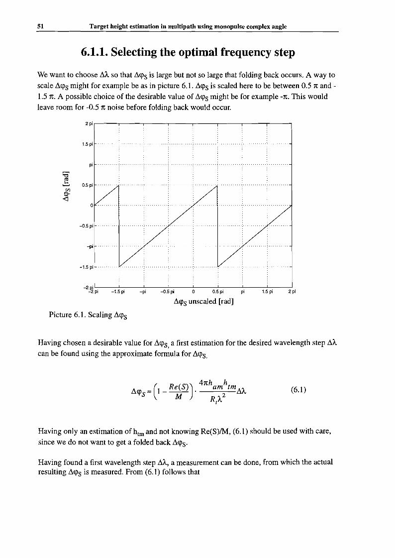
51 Target height estimation in multipath using monopulse complex angle
6.1.1. Selecting the optimal frequency step
We want to choose li.'A. so that li.<ps is large but not so large that folding back occurs. A way to
scale li.<ps might for example be as in picture 6.1. li.<ps is scaled here to be between 0.5 1t and
1.5 1t. A possible choice of the desirable value of li.<ps might be for example -1t. This would
leave room for -0.5 1t noise before folding back would occur.
2pi.---~---.----..-----.---~---.----..------,
1.5 pi
pi
:g~ 0.5 pi
ene<:l
o .
-0.5 pi
-pi
-1.5 pi
-2 p'i L.-_----'-__--'---__...L-__L.-_----'-__--'---__...L.-_-----J
-2 pi -1.5 pi -pi -0.5 pi 0 0.5 pi pi 1.5 pi 2 pi
li.<ps unsealed [rad]
Picture 6.1. Scaling li.<ps
Having chosen a desirable value for li.<ps a first estimation for the desired wavelength step li.'A..can be found using the approximate formula for li.<ps.
(6.1)
Having only an estimation of htm and not knowing Re(S)/M, (6.1) should be used with care,
since we do not want to get a folded back li.<ps.
Having found a first wavelength step li.'A., a measurement can be done, from which the actualresulting li.<ps is measured. From (6.1) follows that

Chapter 6. Algorithm tuning 52
~<pSdesired
~<PSaC1Ual(6.2)
so we can calculate a better desired ~A from the measurement. Care should be taken, becausethe method is subject to three problems:
1. ~<Ps may fold back, in which case (6.2) does not apply.
2. Noise on the measured ~<Ps may cause (6.2) to yield suboptimal values for ~A.
3. Offset on ~<Ps, caused by phase imbalances as described in chapter 4, makes (6.2) inappli
cable, unless compensated for.
To detect folding back, from time to time it should be checked if the found ~<Ps and ~A are
consistent with (6.1).
6.1.2. Finding a frequency range without mispointingdivergence
In chapter 3.1. was derived that in some areas antenna mispointing corrupts the target heightestimate too much to use it for tracking. The range at which these areas occur depends amongstothers on the transmitter frequency. In this section is investigated from simulated data if it ispossible to avoid these areas, by choosing the appropriate frequency. After that an algorithm isproposed to find frequency intervals where no mispointing divergence occurs.
As discussed in section 3.1 the measured target height is unfit for tracking if the height errorcaused by mispointing is larger than the error on the initial height estimate and has the samesign. So if the antenna points one meter above the target, target height measurements up to onemeter above the target are acceptable. In picture 6.1 the simulated target height measurement isplotted against range. The dotted line (...) is obtained using frequencies k1=-32, k2=-28, k3=24,
while the other line (-.-) is obtained using k1=24, k2=28, k3=32. So the two measurements are
on opposite sides of the frequency range.

53 Target height estimation in multipath using monopulse complex angle
2.----rJr.,-,y7TT1r;-r.TTT-----,r--------.-------r------,--------,
60005000400020001000-2o
-1.5
-1
1.5
I1:.~ 0.5.I::
Q)~
~ 0'0Q)
:;lQQ)
E -0.5~eiii
3000R[m]
Picture 6.2. Simulated target height measurement error---- transmitter frequencies k 1 23= -32, -28,-24-.-.- transmitter frequencies k1:2:3 =24,28,32ha= 11 m, ht = 20 m, p=0.6
In the areas where one or both lines are beneath one, measurements of the one beneath one canbe used for tracking. There remain areas where the target height error of both frequency intervals are above one. In these areas we do not have a measurement that can be trusted for tracking. These areas are drawn for different values of the reflection coefficient p in picture 6.3. Ascan be seen in this picture, the higher the reflection coefficient, the better the rnispointingdivergence areas can be avoided.
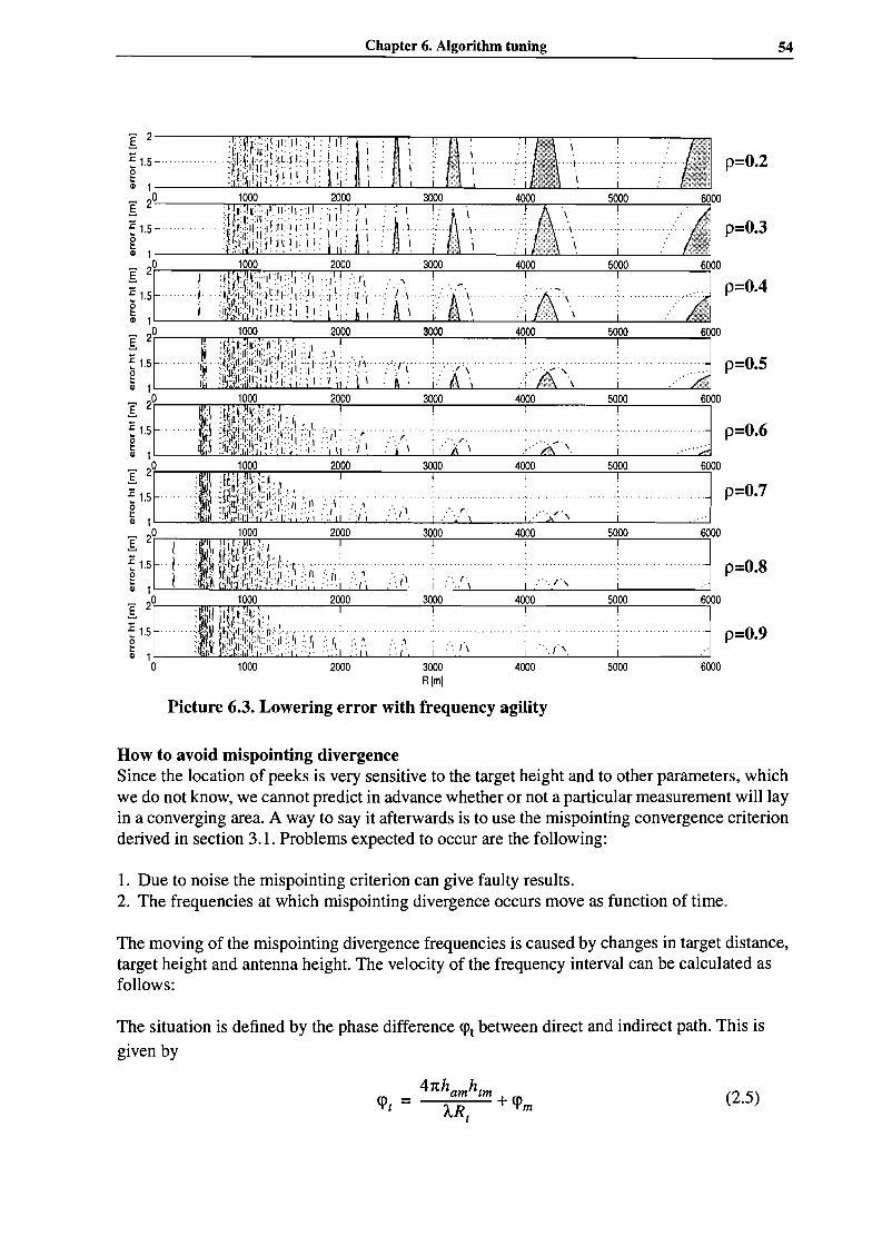
Chapter 6. Algorithm tuning 54
p=O.5
p=O.6
p=O.2
p=O.9
p=O.3
p=O.4
p=O.8
p=O.7
6000
6000
6000
I 2,------:T""'7r"'~:;-:-;-;;-:--1r:_:r...".""T""____:___y_~__,.____nrT--___.,..,._
~ 1.5gIII 1'__ -"""ClWJL...:..J...o...:....:....:.....:...-L....Jl....:.L:...--"-L._....L1.--'-----L.--'--~'___..:.......J..J
~ 2°r-------,T"T"7;r.=.,~:;-':T.-:-;-;--:-:-'~"""'7"T-,....,.-;--=r::-----.....:.::r:.::.....,,____,---=r::_--____:____"'ioS~ 1.5e:D 1'___ ~LJL'-l.L...:....:...:....:..."__'__'----L..J.L:.......II.-L....:..--LJ...--'----L.--""'''____ __~
- 2°i----:-----,'T"'"7m:::..,...,.",c-:"T'...,-,.~rr:,..----~~---...,~---~r_---~oS I~ 1.5 ~.. '. ... \ ~ .
g ~ ,III 1'___~----""""""''''''"''''___~-'--'-___.J.--'--....Il...,;'---.....u.._---''-_J...._...____'__L....L:2~~__L.__...:....:...._
~ 20 5000 6000
oS ~~ 1.5"~III 1 '---_----'l1.I·'---"""""IlL.:..L""'"'-'...:...J...I..'-.L..'-'-....J..L......L.._----U..--'------L:----llJ.........l__----L-Lff.~__l...__.l...___'__~
~ 20r-----;nl-,--:-m7'~~r---=r_:'------"'300=r=_0 4:::;00""'0 .=.:50rOO::__ =60iOOoS~ 1.5 ir .:;. . r.
~ 1'---_----"'''''--"'~1IL.L~'''''--'-.-.L'__':__''>--'-\L..'---,''1,---'_,---:-".-,"___'.1_..1-:1 .~:....L..~"---/___'..,__-----".;_.. ...L..•A;\"".~L·---"·'----_ _L_____'.c:..··_··..<ZJ·~·
- 20r----:'1lIlTT"'"-~Fr_:_---=r_:'------"'300=r=_0 4:::;00""'0 .=.:500r °::-- =60iOOoS I
~ 1.5o ~ .~ 1 '---_-:.:JlJ.<e.....:;;=hL.J.l...-'-'..L.:Ll.:..l.~...1L:.....··!.-I.'___-'-.:..;..·'.1___'.·1._..1...I' -'-.:~·........r...l.., ____11.-:-.._."",.. ~r·___'.'___L ~.:.:...J
_ 20 3000 4000 5000oS I~ 1.5· Ig I /':11 1 .\". .:··.i l. i .. r, i :".1',III 1'---'------""'It:.:..l..~::J.:.l.'-'-'-...:.:.:..L.:.L.........:.~---L.'___~__'__----'-'---"--.l____I._:.._...:.:.........:........__.l..._ ___:_J
-~ ~ ~ ~ ~oS 1 I
~ 1.5
~ 1 '---_--3IJJIL::...l:.;..L:oUL.;l<..::...;...u.:.:J.o...J.:..-:.:.,-,-\L:...::••••.L;,'-',___-,-:.;.j'.i....'· _..I...I' -'-.-'-....~(_,____Ii_.'---·...:.... ',---''-'-' LI' "'"'-oJ
o 2000 3000 4000 5000Rim]
Picture 6.3. Lowering error with frequency agility
How to avoid mispointing divergenceSince the location of peeks is very sensitive to the target height and to other parameters, whichwe do not know, we cannot predict in advance whether or not a particular measurement will layin a converging area. A way to say it afterwards is to use the mispointing convergence criterionderived in section 3.1. Problems expected to occur are the following:
1. Due to noise the mispointing criterion can give faulty results.2. The frequencies at which mispointing divergence occurs move as function of time.
The moving of the mispointing divergence frequencies is caused by changes in target distance,target height and antenna height. The velocity of the frequency interval can be calculated asfollows:
The situation is defined by the phase difference CPt between direct and indirect path. This is
given by
(2.5)
55 Target height estimation in multipath using monopulse complex angle
So if for example the target distance Rt gets 1% smaller, we need approximately a 1% increase
of the wavelength to keep <Pt the same.
For example: let the target distance be 3 km and velocity of the target towards the antenna be300 mls. The target distance gets 10% per second smaller, so the frequency should get 10% persecond smaller to keep <Pt the same. Assuming the initial frequency to be 9 GHz, then the fre-
quency changes at a rate of 900 MHz/s. This is about 11 RF channels per second. Of course atsmaller distances the change would be faster.
The algorithm to find the RF-frequencies should be insensitive to noise and quick enough tokeep track on the moving frequency intervals.
An algorithm to find a mispointing convergent intervalA possible algorithm is the following (picture 6.4)
• At random a RF channel is chosen. A measurement is done with this channel. As long as thernispointing criterion indicates that it is in a diverging area this is repeated.
• If we have a frequency within a converging area, a new frequency interval is created. Thelow and high border are set respectively at the found channel number minus and plus one.
• The interval is evaluated, which means the following:
• measurements are done at the border frequencies. If possible with regard to convergenceand if desirable with regard to the desirable size of the frequency interval, the borders areshifted outwards. If necessary because they have come into a divergence area they areshifted inwards. this is done independently for the upper and lower border.
• The interval is evaluated like that until it is at its maximal size. After that, apart from keeping evaluating the interval, random channels are tried to find a second interval.
• After this is found, both intervals are evaluated each time. In the middle of the largest interval a frequency is chosen for an extra measurement necessary for the target height estimation.
This algorithm has the following features:
• able to find borders of convergence intervals• robust to noise; crossing a border in noise is corrected in the next cycle• whenever there is an interval, three measurements in that interval are available for target
height estimation• keeping track of two intervals, making probable we already have a large second interval
when the first interval disappears from the frequency range• slow at start; corning at maximum size may take 3*64 measurements (worst case)• in steady state independent target height measurements possible at 20 Hz.• unable to handle shrinking desired wavelength interval
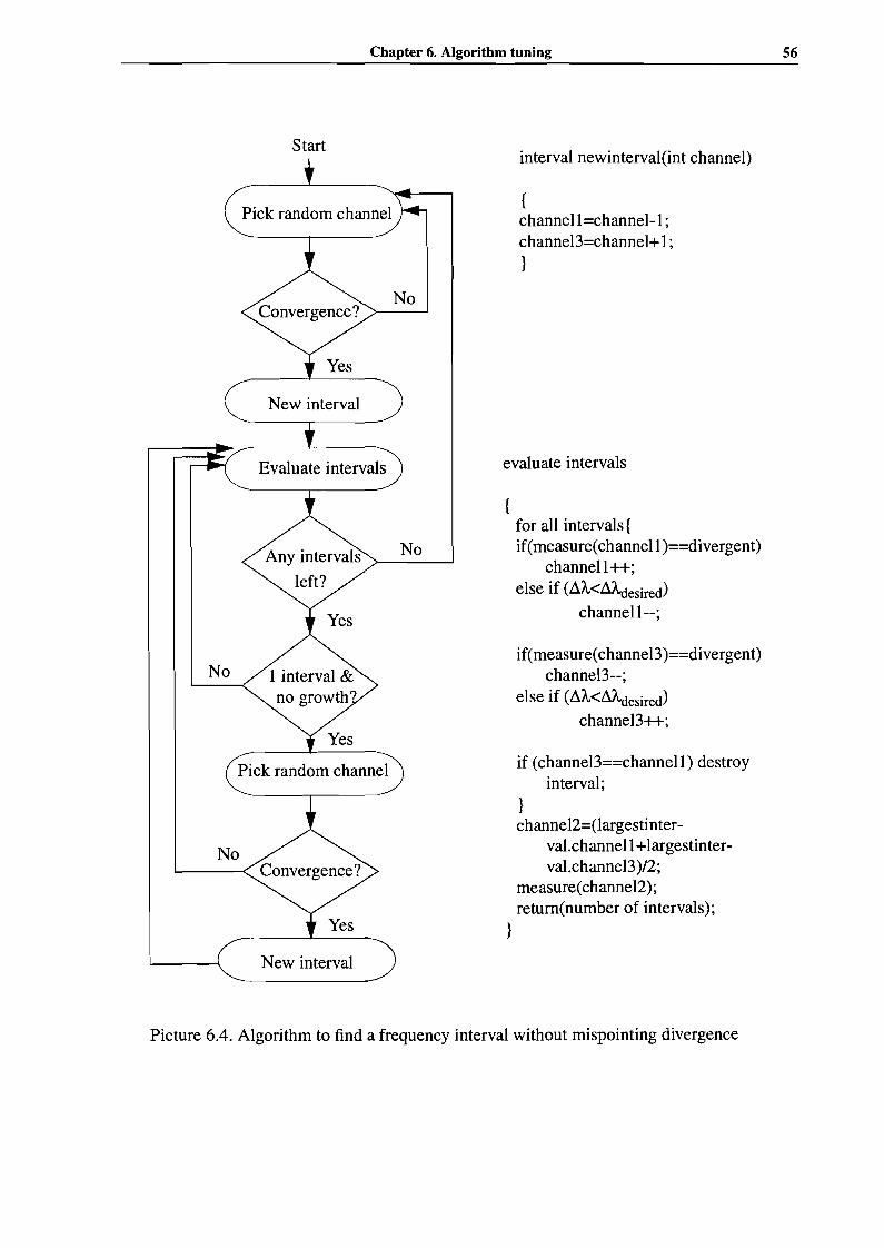
Start
Chapter 6. Algorithm tuning
interval newinterval(int channel)
56
No
Pick random channel
Yes
New interval
Evaluate intervals
I interval &no growth?
Yes
Pick random channel
No
No
{channell =channel-l ;channe13=channel+I;}
evaluate intervals
{for all intervals {if(measure(channell )==divergent)
channell ++;else if (~A.<~A.desired)
channel1--;
if(measure(channe13)==divergent)channe13--;
else if (~A.<~A.desired)
channe13++;
if (channe13==channell) destroyinterval;
No
New interval
}channeI2=(largestinter
val.channell+largestinterval.channe13)/2;
measure(channel2);retum(number of intervals);
}
Picture 6.4. Algorithm to find a frequency interval without mispointing divergence
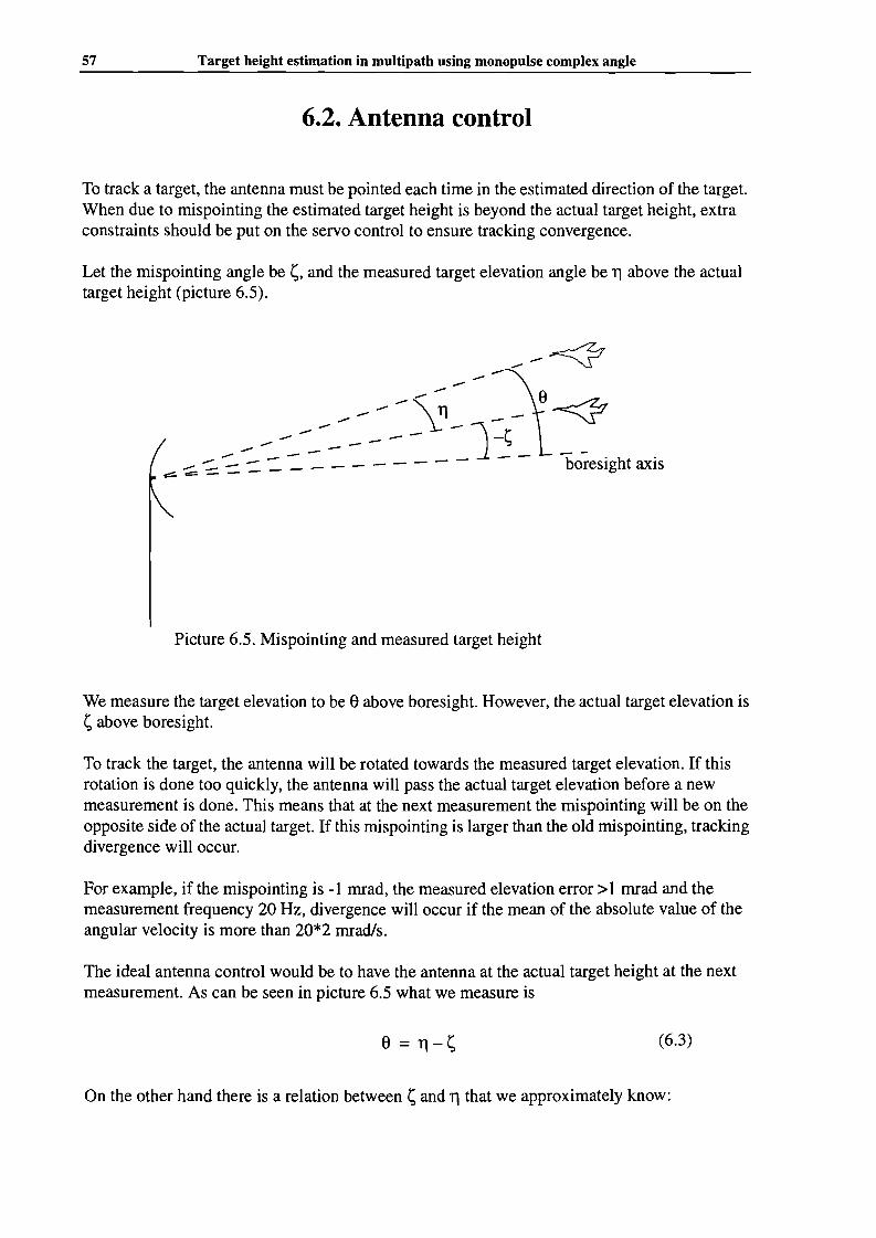
57 Target height estimation in multipath using monopulse complex angle
6.2. Antenna control
To track a target, the antenna must be pointed each time in the estimated direction of the target.When due to mispointing the estimated target height is beyond the actual target height, extraconstraints should be put on the servo control to ensure tracking convergence.
Let the mispointing angle be ~, and the measured target elevation angle be 11 above the actualtarget height (picture 6.5).
--~
_-----~:)-~2le~- - -Y-""" -- "='
-""" - - -_ -::::. -:. - -:. -=- _ - - - - - - - - - boresight axis~-==---
Picture 6.5. Mispointing and measured target height
We measure the target elevation to be eabove boresight. However, the actual target elevation is~ above boresight.
To track the target, the antenna will be rotated towards the measured target elevation. If thisrotation is done too quickly, the antenna will pass the actual target elevation before a newmeasurement is done. This means that at the next measurement the mispointing will be on theopposite side of the actual target. If this mispointing is larger than the old mispointing, trackingdivergence will occur.
For example, if the mispointing is -1 mrad, the measured elevation error>1 mrad and themeasurement frequency 20 Hz, divergence will occur if the mean of the absolute value of theangular velocity is more than 20*2 mrad/s.
The ideal antenna control would be to have the antenna at the actual target height at the nextmeasurement. As can be seen in picture 6.5 what we measure is
e=11-~ (6.3)
On the other hand there is a relation between ~ and 11 that we approximately know:
Chapter 6. Algorithm tuning 58
So
= htm yk == cRt 1- Re(S)
M
(3.7)
11 = c~
In which c is the mispointing criterion, which can be measured. Now we can solve for ~:
e~=-...,-
(c - I)(6.4)
So it is theoretically possible to calculate the mispointing angle from measurements. In practice, when c is close to unity (6.4) will yield unusable solutions, because errors on ewill beamplified. When c is negative, as is the case in picture 6.5, (6.4.) will yield a usable estimationof the mispointing angle. If the mispointing criterion can be estimated from measurementsaccurate enough, this may also be useful to calculate the target height more accurate.
The optimal antenna angular velocity is the velocity that would make the mispointing anglezero in one measurement. The maximal antenna angular velocity, at which the system is at theborder between convergence and divergence, is twice that speed.
59 Target height estimation in multipath using monopulse complex angle
7.1. Conclusions
Analysis and simulation
Mispointing, diffuse reflection, glint, quantisation noise and phase measurement noise havebeen modelled. The most important error sources are mispointing, diffuse reflection and glint.Due to diffuse reflection, the complex angle method will not work good at high sea states andtargets at higher elevations. Due to glint, the complex angle method will not work good at largetargets.
A height measurement can best be done with three measurement frequencies. Taking the measurement frequencies further apart will reduce most errors, but may lead to a larger integrationerror near peaks in the real part of the monopulse ratio. Taking the measurement frequenciesfurther apart is often not possible due to mispointing divergence.
At some areas mispointing causes tracking divergence. These areas are near peeks in the realpart of the monopulse ratio. A criterion has been derived to deduct from a measured valuewhether or not it is in such a divergence area. In many cases it is possible to avoid divergenceareas by choosing an appropriate transmitter frequency. An algorithm to do this has been proposed.
There probably exist phase imbalances between ~ and L channel, causing systematic errors inthe target height measured with complex angle. The size of these phase imbalances is unknownas is the way in which they depend on frequency, temperature and time. An experiment featuring a free space target that is tracked off boresight, has been proposed to investigate this.
Low target measurements
Low target measurements that were done at sea in 1991 have been processed. The results leadto the following conclusions:
Larger targets and higher flying targets give indeed worse results than smaller and lower targets.
The model for diffuse reflection is at least qualitatively correct.
In some runs and at some distances the measured mispointing criterion is above or belowthreshold for longer times, which means that the signal to noise ratio on the mispointing criterium is large. Whether or not the measured mispointing criterion corresponds to the actualeffect of mispointing remains to be tested.
In two test runs the correct target height is found in some areas with an RMS error of 5 m. Lowpass filtering may improve the result.
There are spiky areas in the measured phase difference, that remain unexplained. At theseareas, the target height and mispointing criterion are spiky too.

Chapter 7. Conclusions and recommendations 60
General conclusionIf the existing problems like phase imbalances are solved, measuring target height with complex angle may be useful for small, low flying targets at smooth sea. An accuracy of RMS 5 mat a measurement frequency of 20 Hz seems to be possible.
7.2. Recommendations
Future investigation on target height estimation using complex angle might consist of the following steps
1. Investigating phase imbalances:
Perform off boresight free space measurement as described in chapter 4.A way to calibrate these phase imbalances is to be developed.
2. Investigating mispointing and the mispointing criterion:Rushton at 10 m height. Large fixed frequency interval. Video tracking with known, small mispointing angle.
Rushton at 10 m height. Large fixed frequency interval. Video tracking with zero mispointingangle.
These measurements should confirm the theoretical analysis of the effects of mispointing andshould give an indication on the noisiness and usability of the mispointing criterion.
3. Developing a frequency choice algorithmHaving developed a usable mispointing criterion, a transmitter frequency choice algorithm canbe made. This should be tested with simulations and measurements:
Rushton at 10 m height. Frequency selection by means of frequency choice algorithm. Videotracking.
Other interesting measurementsTo see the effect of glint and diffuse reflection, the following measurements would be interesting:
1. Rushton at 10m height. Video tracking.
2. Rushton at 20 m height. Video tracking.
3. F-16 at 20 m height. Video tracking.
Differences between 1 and 2 will be mainly due to diffuse reflection.Differences between 2 and 3 will be mainly due to glint.
61 Target height estimation in multipath using monopulse complex angle
All measurements should be at low sea states, typically smaller than sea state 3. The followingquantities should be registered:• Actual target height• Target distance• Real and Imaginary part of ~E and L• Antenna pointing direction• Transmitter frequency• Phase imbalance correction
Further analysis:
Using a more realistic model for diffuse reflectionSpecular reflection is also statistical, with a decorrelation time of seconds, but a small autocorrelation between different transmitter frequencies This should introduce errors in the targetheight measurement.
Modelling glint more realistic, with respect to its time behaviour (autocorrelation function).
Explaining the spikes observed in the measured ~q>s.
Investigating how the measurements can best be filtered.

Literature
Literature
Books:
[Shennan 84]Shennan,S.M., MONOPULSE PRINCIPLES AND TECHNIQUES.London: Artech house, 1984
[Leonov 86]Leonov, A.I. and K.I. Fomichev, MONOPULSE RADAR.Norwood: Artech house, 1986, Translated from Russian
[Beckmann 63]Beckmann, P. and Spizzichino, A., THE SCATTERING OF ELECTROMAGNETIC WAVES FROM ROUGHSURFACES.Oxford; Pergamon press, 1963
Papers:
62
[Daeipour 97]Daeipour, E and W.D. Blair, Y. Bar-shalom, BIAS COMPENSATION AND TRACKING WITH MONOPULSERADARS IN THE PRESENCE OF MULTIPATH.IEEE transactions on Aerospace and Electronic Systems, Vol. 33 (1997), Iss. 3, P 863-882
[Eckersten 92]Eckersten, C, RADAR TRACKING OF SEA SKIMMERS, AN IMPLEMENTATION OF COMPLEX ANGLE.lEE Conference Publications n. 365 (1992), p 46-49
[Nakatsuka 90]Nakatsuka, K, TWO-BEAM TECHNIQUE FOR TRACKING A TARGET AT LOW ELEVATION ANGLES.lEE Proceedings F ( Radar and Signal Processing) Vol. 137 (1990), Iss. 6, p 397-406
[Wang 96]Wang, Xiqin and Peng, Yingning ; Ma, Zangue, ALGORITHM BASED ON ELEVATION GEOMETRIC MEANFOR MONOPULSE RADARS TO TRACK A TARGET AT LOW ALTITUDE.Proceedings of the 1996 CIE Int. Conference of Radar Proceedings, ICR'96, p 739-742
[Lo 90]Lo, T and J. Litva, MULTIPATH PROPAGATION EFFECTS ON LOW-ANGLE RADAR TRACKING: ANEXPERIMENTAL EVALUATIONAP-S International Symposium v. 4 (1990), P 1816-1819
[Lo 91]Lo, T. and J. Litva, CHARACTERISTICS OF DIFFUSE MULTIPATH AT LOW GRAZING ANGLES INNAVAL ENVIRONMENTS.International Geology and Remote Sensing Symposium v. 3 (1991), P 1259 - 63
[Beard 61]Beard, C.I., COHERENT AND INCOHERENT SCATTERING OF MICROWAVES FROM THE OCEAN.IRE Trans. Ant. Prop., vol AO-9, (sept. 1961) p 470-483
[Barton74]Barton, B.K., LOW ANGLE RADAR TRACKING.IEEE Proceedings, Vol. 62, n. 6, (june 1974) p 687-704

63 Target height estimation in muItipath using monopulse complex angle
[Symonds 73]Symonds, M.D. and J.M. Smith, MULTI-FREQUENCY COMPLEX ANGLE TRACKING OF LOW LEVELTARGETS.Proceedings of the lEE International Conference on Radar, Oct. 1973
[Sherman 71]Sherman, S.M., COMPLEX INDICAlED ANGLES APPLIED TO UNRESOLVED RADAR TARGETS ANDMULTIPATH.IEEE transactions on Aerospace and Electronic Systems, Vol. 7 (1971), No I.
[Howard 74]Howard, D.D. and S.M. Sherman, D.N. Thomson, J.J. Campbell,EXPERIMENTAL RESULTS OF THE COMPLEX INDICAlED ANGLE lECHNIQUE FOR MULTIPATHCORRECTION.IEEE transactions on Aerospace and Electronic Systems, Vol. 10 (1974), No 6.
Signaalliterature
[Nooy],Nooy, P.N.C., DOELSIGNATUREN & MEETINSTRUMENlEN.DNCS-Analyse
[de Vries 88]De Vries, J. and P.N.C. Nooy, DIFFUSE REFLECTIE BIJ MULTIPATH.MEMO PrAlAnalyse, 1 feb. 1988
[Maas 97]Maas, AJ. and E.R. Stolp, INVENTARISATIE VAN OPLOSSINGEN VOOR HET LAAGDOEL-PROBLEEM.R&S-FD-DAP, 21 jan. 1997
[Rotgans 88]Rotgans, P., INZICHT IN LAAGDOELFENOMEEN EN OPLOSSINGEN VAN DIT PRO-BLEEM.MEMO SEAT Nr. 667, 29 jan. 1988
[Setyowati 92]Setyowati, A.E., EVALUATIE VAN RADARMETINGEN IN EEN MULTIPATH OMGE-VING.Traineeship report, supervisor MJ.S. van Ommeren, 31 may 1992
[Bongers 92]Bongers, P.P.M., UITWERKING LAAGDOELMETINGENTraineeship report, supervisor M.J.S. van Ommeren, october 1992

Appendix At. Symbols
Appendix Al List of symbols
A=radius of the earth 0:= 6372 kmA = integrand of (2.23)FE(8) = error voltage from direction 8
G = pGS(8m)/GS(8t ) = effective reflection coefficient in the mirror direction
Gs , GE = Antennapattem of the Sum and Elevation channel
ha, ht = Antenna height and target height with respect to the earth surface
ham ,htm = Antenna height and target height with respect to the plane of reflection
hah ,hth = Height of the plane of reflection near the antenna and near the target
M=FE(8m) = error voltage from the mirror
Rt = target rangeS = /)J'f, = monopulse quotientT=FE(8t) = error voltage from the target
ex = grazing angley = factor accounting for the influence of mispointing on d<Ps/<pt
Ll = difference signalLl<Ps = phase change of the monopulse quotient SEc = dielectric constant of reflecting surface
8m= the angle between the mirrored target and the boresight-axis
8t = the angle between the target and the boresight-axis
A = transmitter wavelength~=RtA
p = The reflection coefficient of the reflecting surfacePo = Fresnel reflection coefficient for a smooth surface
Pd = Diffuse scattering coefficient
Ps = Specular scattering coefficient
'f, = sum signal<Pm = additional phase shift that occurs in reflection at sea surface.<Ps = phase of the monopulse ratio<Pt = phase difference <Pt between the direct and indirect signal.
64

65 Target height estimation in multipath using monopulse complex angle
Appendix A2 Integration of three measurements
Let three measurements, (xl,yl), (x2,y2) and (x3,y3) be given. We want to approximate the integral
x3
f ydx
xl
First fit a parabole through the measurement points:
y = ax2 + bx + c
Filling in the measurement points and solving the resulting three equations gives
b = (yl-y3)(x1 2-x22)-(yl-y2)(x1 2-x3 2)
(xl-x3)(x1 2-x22)-(xl-x2)(x1 2-x32)
(A2-1)
(A2-2)
(A2-3)
a =(yl-y2)-b(xl-x2)
(x1 2-x22)(A2-4)
c = yl-ax1 2 -bxl
Having calculated the coefficients of the parabole, the integration can be done
x3 x3
f ydx""'- f(ax 2 +bx+c)dx = ~(X33-x13)+~(X32-x12)+C(X3-Xl)xl xl
(A2-5)
(A2-6)

Appendix A3. Derivation of y
Appendix A3 Derivation of y
In chapter 3 it was stated that the phase relation with antenna rnispointing was
(3.3)
66
(A3-I)
(A3-2)
In this equation S is the monopulse quotient, <Ps is the phase of S, M=FE(Sm) is the error voltagein the direction of the mirror, T=FE(St)is the error voltage in the direction of the target. According to (3.2), the exact expression of 'Y is
(GMcoscpt + T) (Gcoscpt + 1)'Y = - ------~
M 2G2 + 2TGMcoscpt + T2 M(l + 2Gcoscpt + G2 )
In which the effective reflection coefficient in the mirror direction G = pGS(Sm)/GS(St).The purpose of this derivation is to express 'Y in terms of measurable quantities, such as Re(S),Im(S), <Ps and S. First look at the first term of (A3-1), which we will call A
(GMcoscpt + T)A=---:-----:---------:
M 2G2 + 2TGM COs CPt + T2
Looking at (2.16) and (2.17) we can derive the following expression
GsinCPt(T - M) . 2
Im(S) _ 1 + 2Gcoscpt + G =
ISj2 - [ Gcoscpt + G2
]2 [ GSincpt]2T-(T-M)· + (T-M)·----~
1+ 2Gcoscpt + G2
1 + 2Gcoscpt + G2
(T - M)GsinCPt= ----.,.---------.,,-
M 2G2 + 2TGMcoscpt + T2 (A3-3)
(A3-4)
Note that (A3-3) has the same denominator as (A3-2). However, the numerator of (A3-2) wesee a cosinus, whereas in the numerator of (A3-3) there is a sinus. The following goniometricequation enables us to write a cosinus as the difference of two sinuses.
(a +~) _sin a - sin ~cos -- -
2 2sin(a~ ~)
If we measure S at three equidistant frequencies, we will have measurements in which <Pt takesthree values. Applying (A3-4) and filling in a=<Pt3 ~=<Ptl and (a+~)l2=<Pt2 it follows. .
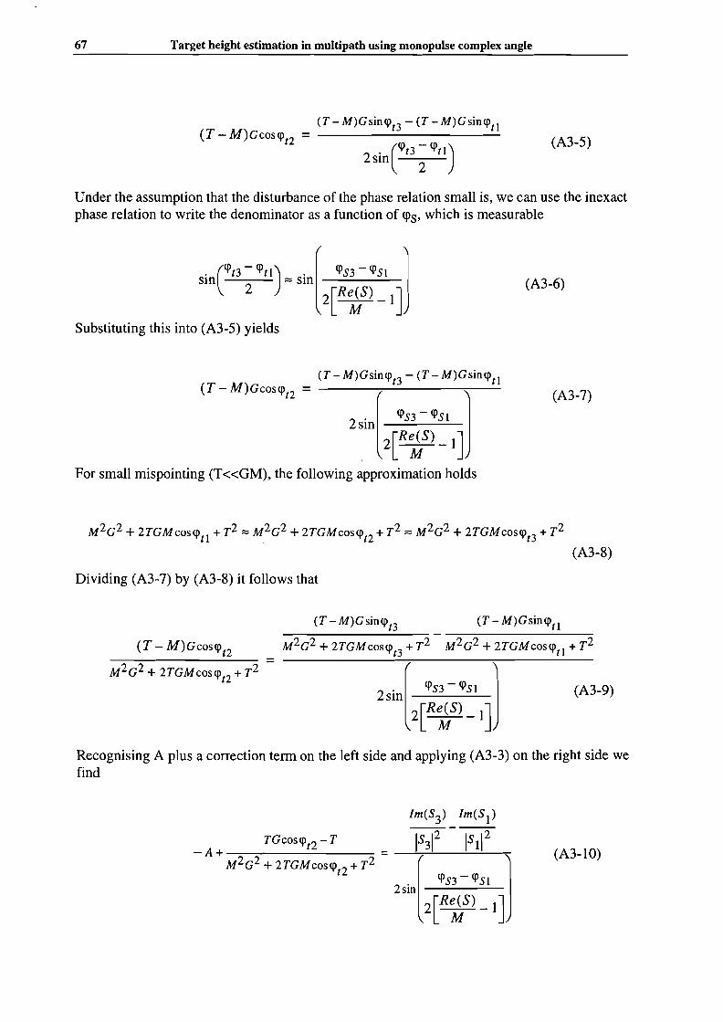
67 Target height estimation in multipath using monopulse complex angle
(T - M)GsinCPt3 - (T - M)GsinCPtl(T-M)GcosCPt2 =-----------
. (CPt3 - CPtl)2slO 2
(A3-5)
Under the assumption that the disturbance of the phase relation small is, we can use the inexactphase relation to write the denominator as a function of <Ps, which is measurable
(T - M)GcosCPt2 =
. (CPt3 - CPtl) . [ CPS3 - CPSi JSIO 2 =SIO
2[R~S) -1]
Substituting this into (A3-5) yields
(T - M)GsinCPt3 - (T - M)GsinCPtl
2SiO[2[~~\ ]]For small mispointing (T«GM), the following approximation holds
(A3-6)
(A3-7)
M2G2 + 2TGMcoscp + T2 =M2G2 + 2TGMcoscp + T2 =M2G2 + 2TGMcoscp + T2tl. t2 t3
(A3-8)
Dividing (A3-7) by (A3-8) it follows that
(T - M)GcosCPt2=
(T - M)GsinCPt3 (T - M)GsinCPtl
M2G2 + 2TGMcosCPt3 + T2 M2G2 + 2TGMcosCPtl + T2
2SiO[2[~~1 I]] (A3-9)
Recognising A plus a correction term on the left side and applying (A3-3) on the right side wefind
(A3-lO)
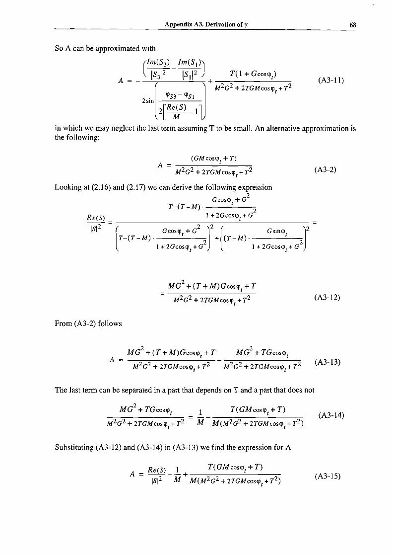
Appendix A3. Derivation of 'Y
(A3-11)
68
(A3-2)
in which we may neglect the last term assuming T to be small. An alternative approximation isthe following:
(GMcos<Pt + T)A = ----::----::-------::
M2G2 + 2TGMcos<Pt + T2
Looking at (2.16) and (2.17) we can derive the following expression2
Gcos<Pt + GT-(T-M)· 2
Re(S) 1 + 2Gcos<Pt + G
1Si2=[T_(T_M). GCOS<Pt+G2
J2
+[(T-M). Gsin<Pt J2=1 + 2Gcos<Pt + G
21 + 2Gcos<Pt + G
2
2MG + (T + M)Gcos<Pt + T
= ---:=---:=----------;:--
M2G2 + 2TGMcos<Pt + T2
From (A3-2) follows
(A3-12)
2MG + (T + M)Gcos<Pt + T
A =M2G2 + 2TGMcos<Pt + T2
2MG + TGcos<Pt
(A3-l3)
The last term can be separated in a part that depends on T and a part that does not
Substituting (A3-12) and (A3-14) in (A3-l3) we find the expression for A
Re(S) 1 T( GM cos<Pt + T)A = -- - - + --::--::-------___=_
ISI 2 M M(M2 G2 + 2TGM cos <Pt + T2)
(A3-14)
(A3-1S)
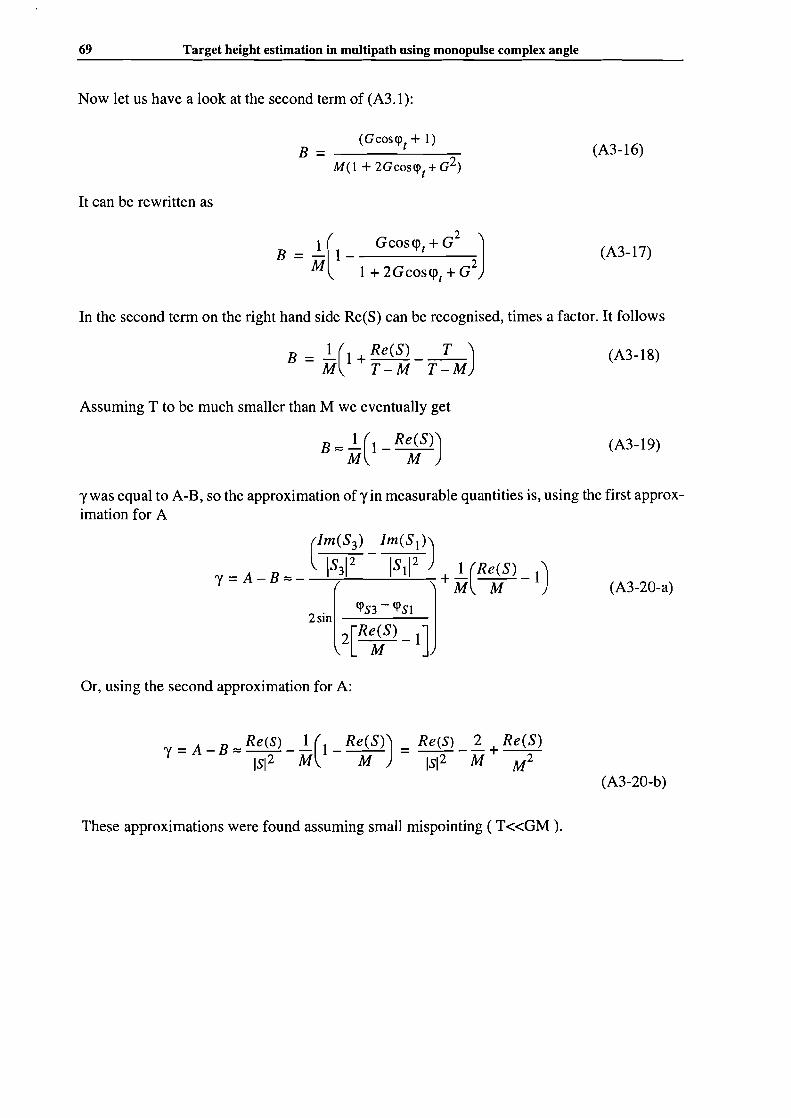
69 Target height estimation in multipath using monopulse complex angle
Now let us have a look at the second term of (A3.I):
(GCOSCPt + 1)B = -------:-
M(l + 2GcosCPt + G2)
It can be rewritten as
[2 J1 Gcos<j)t + G
B = M 1 - 1 + 2Gcos<j)t + G2
(A3-I6)
(A3-17)
In the second term on the right hand side Re(S) can be recognised, times a factor. It follows
B = 1-(1 + Re(S) _ _ T_)M T-M T-M
Assuming T to be much smaller than M we eventually get
(A3-I8)
(A3-I9)
"(was equal to A-B, so the approximation of"(in measurable quantities is, using the first approximation for A
Or, using the second approximation for A:
(A3-20-a)
(A3-20-b)
These approximations were found assuming small mispointing (T«GM ).
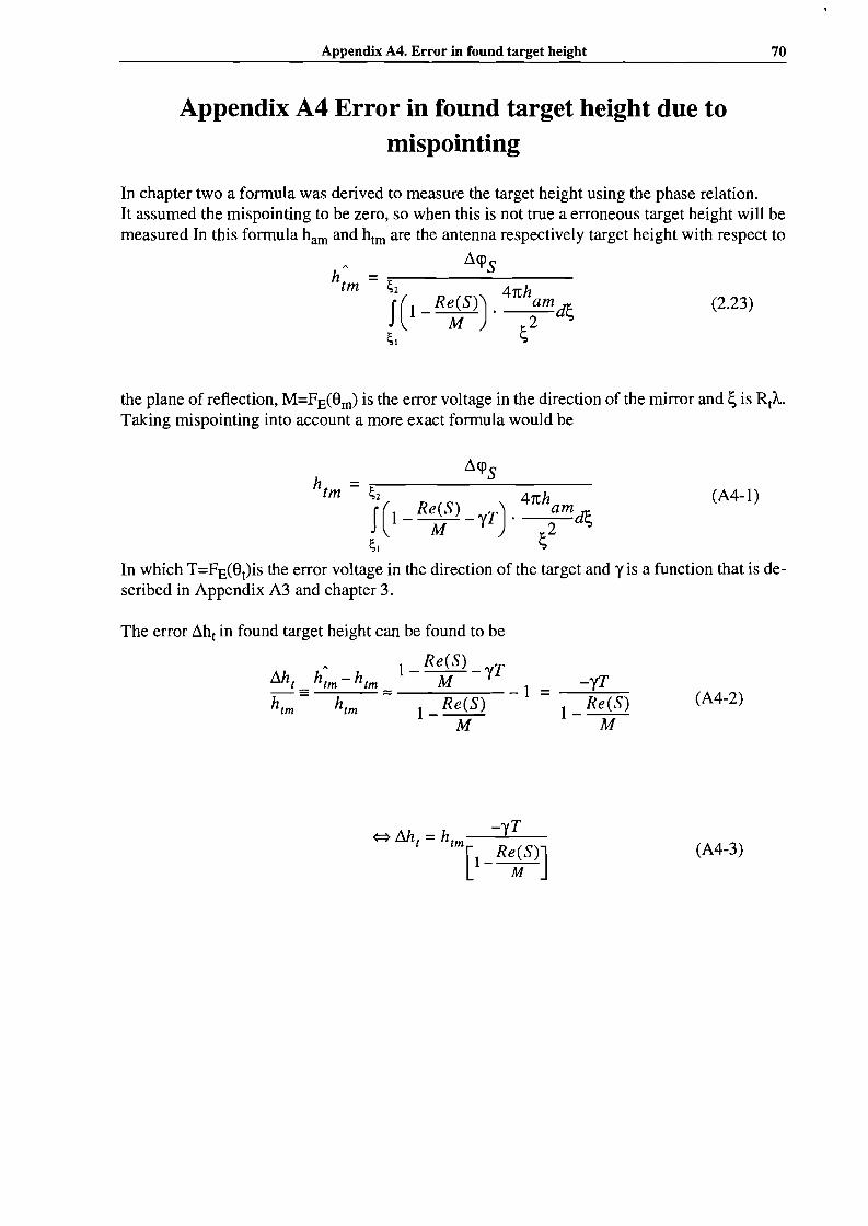
Appendix A4. Error in found target height
Appendix A4 Error in found target height due tomispointing
70
(2.23)
In chapter two a formula was derived to measure the target height using the phase relation.It assumed the mispointing to be zero, so when this is not true a erroneous target height will bemeasured In this formula ham and htm are the antenna respectively target height with respect to
A Ll<pSh -;;----------tm - ;2 41th
f(I-R~S)). r-;md~;\ ~
the plane of reflection, M=FE(Sm) is the error voltage in the direction of the mirror and ~ is RtA.Taking mispointing into account a more exact formula would be
Ll<PSh = ;;------------
tm ;2 41th (A4-1)f(l- Re(S) -YT). amd~
M r-2;[ ~
In which T=FE(St)is the error voltage in the direction of the target and Yis a function that is described in Appendix A3 and chapter 3.
The error Llht in found target height can be found to be
(A4-2)
(A4-3)
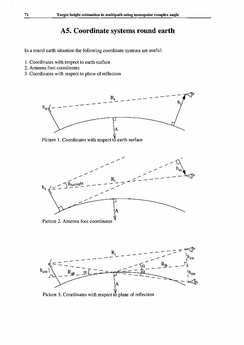
71 Target height estimation in multipath using monopulse complex angle
AS. Coordinate systems round earth
In a round earth situation the following coordinate systems are useful:
1. Coordinates with respect to earth surface2. Antenna foot coordinates3. Coordinates with respect to plane of reflection
Rt----- -
Picture 1. Coordinates with respect t earth surface
Picture 2. Antenna foot coordinates
---:;:;::~Rt _ - - - - -- -- ,
-------- ------ ,~--- ~
__ -- --a. Rth r+R L - - ~::: - - - - - - 'h
tmah a. _~..;:-::..._,~-~_=-_--JJJL
----- I- - ..I«?
Picture 3. Coordinates with respect t plane of reflection

Appendix AS. Coordinate systems round earth 72
Assuming the radius of the earth A to be large compared to the distance Rt and the target height
small compared to the distance Rt the following coordinate transformations may be used:
Between antenna foot and earth coordinates:
Assuming hta to be parallel to ht,Pythagoras theorem yields
(A5-I)
Between reflecting surface and earth coordinates
- ---------ham \ Rah a L =--
.l -----
hath
Picture 2.3. Multipath geometry
In this picture the symbols are the following:ha, ht = Antenna height and target height with respect to the earth surface
ham ,htm = Antenna height and target height with respect to the plane of reflection
hah ,hth = Height of the plane of reflection near the antenna and near the target
a = grazing angleA=radius of the earth
Usually the antenna height ha and ( an estimation of) the target height ht are known.We can
then calculate the height of the reflection plane using the following derivation. Pythagoras theorem states that
in which A is the radius of the earth = 6372 km. Because A»hah it follows:
In a similar way can be derived that
(A5-2)
(A5-3-a)

73
Thus
Target height estimation in multipath using monopulse complex angle
(A5-3-b)
(A5-4)
(A5-5)
Assuming ht to be of equal size as ha,
hth hah
h;=-';;;Combining this with (A5-4) gives for the height of the reflecting plane at the antenna and at thetarget
hah = Rt2
2A [I +ft:J'hth = Rt
2
2A.[I+ ~J'
(A5-.6-a)
(A5-6-b)
and finally we find the expressions for the antenna and target height with respect to the reflecting plane to be
(A5-.7-a)
(A5-.7-b)
The latter equations have been derived under the assumption that ha = ht• If ht«ha small errors
may occur. In picture A5-1 for example the plane of reflection is tilted to much counter clock
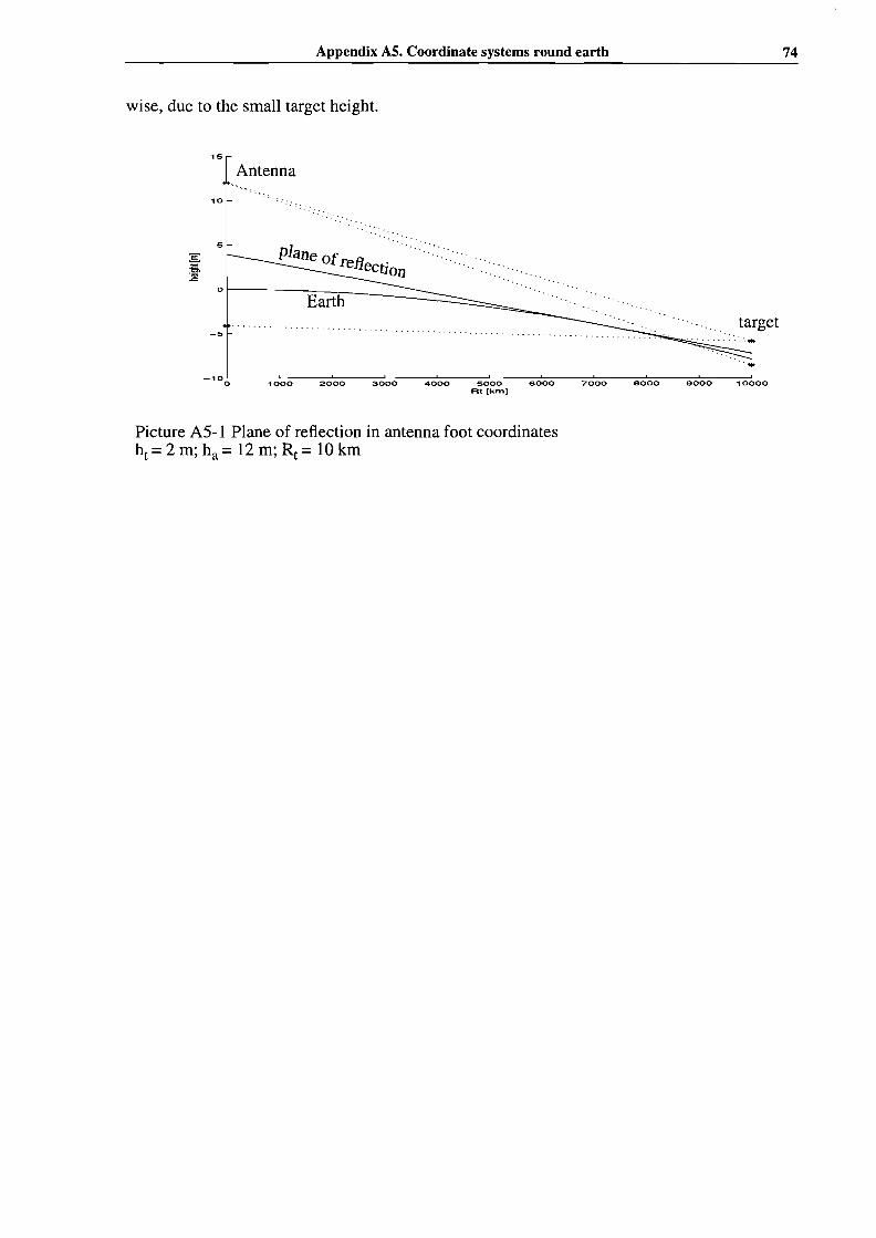
Appendix AS. Coordinate systems round earth 74
wise, due to the small target height.
1S
Antenna......
10 -;;
::::::::::::. "'.
target
plane ofrefl .' .ectlon
o r--REaafirtthh----==::::::::=::::::::=::::::.:::::=~····:·:'.
S
-S
-1 0 O~-----=-10='=0::-::0,--------:2=-=0'="00=---=c30=':0=-=0------:4:::'0'::-,00=---S=-=0:'=0=0-----=e-::00=-=0=-------:7::-::0~0=co-----:::-eo='=o:c:o,--------:g=-=o'="o=co---=1~OOOOAt [krn)
Picture A5-1 Plane of reflection in antenna foot coordinatesht =2 m; ha =12 m; Rt =10 km

75 Target height estimation in muItipath using monopulse complex angle
Appendix B Listings
Bl The simulator
The simulator simulates measurements with a monopulse radar under multipath conditions. Itconsists of a part that simulates the propagation path, a part that performs the monopulse measurement and a part that performs the calculations to estimate target height using complex angle.In the first two parts different noise sources can be added
The simulator consists of the following matlab scripts and functions
• menu.m• calcsim.m• plotten.m• monopuls.m• gel.m• gs.m• fe.m• integrate.m
menu.m draws a user interface. In this user interface the user can adjust the following:• quantities are to be plotted (target height measured with complex angle, error of the former,
~<Ps, target height measured with conventional monopulse method, specular reflection coefficient )
• upper and lower value of the plots• Geometrical situation (target height, antenna height, wave height / reflection coefficient,
transmitter frequency channels)• Error sources (mispointing height, noise dphi, height glint, distance glint, quantisation
noise, diffuse reflection ).• By clicking 'Plot' the simulation is done using 'calcsim.m' and the results are plotted using
'plotten.m' .• By clicking 'Clear' the screen is cleared.Input: noneOutput: a set of global variables that correspond with the user adjustments on the menu.
calcsim.m performs the simulation. The geometrical situation is transformed to reflecting planecoordinates. Mispointing is added. With 'monopuls.m' simulated measurements are done. Glintand receiver errors are added. The target height is calculated.Input: a set of global variables that correspond with the user adjustments on the menu.Output: a set of global variables with simulation results
plotten.m plots all selected quantities.Input: global variables corresponding with user adjustments on the menu, simulation resultsOutput: none
Appendix B Listings 76
monopuls(R,ha,ht,lambda,thetaborsight,waveheight,rho,tixedrho,diffusereflection)gives a simulated monopulse measurement. If fixedrho==l then p is taken rho, else it is calculated from the waveheight. If diffusereflection==1 then diffuse reflection is added.Input: Target distance, antenna height, target height, transmitter wavelength, borsight angle,RMS wave height, reflection coefficient, fixedrho, diffusereflectionGeometric properties are in reflecting plane coordinatesOutput: delta signal, sum signal, specular reflection coefficient
gel(theta,lambda)gives the antenna gain of the delta elevation channel in the direction theta at transmitter wavelength lambda.
gs(theta,lambda)gives the antenna gain of the sum channel in the direction theta at transmitter wavelength lambda.
fe(theta,lambda)gives the error voltage in the direction theta, which is per definition equal togel(theta,lambda).Igs(theta,lambda)
integrate(xl,x2,x3,yl,y2,y3)x3approximates the integral Jydx from three points.
xl
B2 Processing registered measurements
Processing a registered measurement can be done as follows:
load the measurement, by typing for example: ' load run121205'adjust the value HIGH and LOW in the listing of proces.mThese values indicate the highest and lowest sample number of the measurement. They can beobtained by looking at the 100 Hz target distance measurements tmtutg.
For example:type 'plot(tmtutg);' (see picture B-2)
In this picture we can see that the measurement went from 3500 m to 500 m distance, corresponding approximately with sample numbers 4200 till 6000. So HIGH=6000 and LOW=4200would be a good adjustment for this measurement.
proces.m calculates and plots target height using conventional monopulse, ~<ps,target heightusing complex angle and the mispointing criterium.

77 Target height estimation in multipath using monopulse complex angle
12oo0,----,..-------r------,,----.,-----.-----,-------,
10000
8000
6000
4000
2000
00L---1--'OO-0---2...L00-0 --:-::3QLOO,-------4"'00=-=-0---=-so::':-00---6QO=0:-----=7000
Picture B-2 target distance tmtutg versus sample number
B3 Listings
menu.m
fig=figure; % nieuwe figuurset(fig,'Color',[0,0.2,0.4D;plots=[ 1,1,1,1,0];ha=11 ;htc=20;goltboogte=0.301; rho=0.6; rhopopup=O; fixedrho=O;mins=[O,-lO,-pi,O] ;maxs=[40,1O,pi,150];mispointing=O;ruisdphisigma=O;ruisht=O;ruisRt=O;quantisatieruis=O;diffusereflectie=O;channel=[0,8,16];linestyle=";
pl1=0;pI2=0;p13=0;pI4=0;pI5=0;% handles naar plaatjes zijn aanvankelijk nul
uicontrolCStyle','frame','Units','normalized','Position',[0,0,0.31,1 D;

Appendix B Listings 78
uicontrolCStyIe', 'Pushbutton','Units', 'nonnalized' ,'Position',[0,0,0.095,0.1], 'String','Plot' ,'Callback', 'plotten;');uicontrolCStyIe' ,'Pushbutton','Units' ,'nonnalized', 'Position',[0.1,0,0.095,0.1], 'String', 'Clear','Callback', 'if (pI1),delete(pll);pll=O;end; if(pI2),delete(pI2);pI2=0;end; if (p13),delete(p13);p13=O;end; if (pI4),delete(pI4);pI4=0; end; if(pI5),delete(pI5);pI5=0;end;');uicontrolCStyle','text','Units','nonnalized', 'Position',[0.2,0,0.095,0.1] ,'String', 'linestyIe');linestyleedit=uicontroICStyle','edit','Units','nonnalized','Position',[0.2,0,0.095,0.05],'String',linestyle,'Callback','Iinestyle=get(linestyleedit,"String");');
x=[O.OI,O. 105,0. 1525,0.2];y=[0.9,0.85,0.8,0.75,0.71,0.67];
uicontroICStyle','frame','Units','nonnalized','Position',[O.005,0.72,0.30,0.28]);uicontroICStyle', 'text' ,'Units' ,'nonnalized','Position',[x(1),0.95,0.095,0.04], 'String', 'Plot');ch1=uicontrolCStyIe', 'checkbox','Units', 'nonnalized' ,'Position', [x(1),y(1),0.095,0.05], 'String','ht','Value',plots(1),'Callback', 'plots(1)=get(ch I,"Value");');ch2=uicontrolCStyIe', 'checkbox','Units','nonnalized', 'Position' ,[x(1),y(2),0.095,0.05], 'String','Error ht', 'Val-ue',plots(2),'Callback','plots(2)=get(ch2,"Value");');ch3=uicontrolCStyIe', 'checkbox','Units', 'nonnalized' ,'Position',[x(1),y(3),0.095,0.05] ,'String', 'dphi','Value',plots(3),'Callback','plots(3)=get(ch3,"Value");');ch4=uicontroICStyle','checkbox','Units','nonnalized','Position',[x(I),y(4),0.095,0.05],'String','htmonopuls','Value',plots(4),'Callback', 'plots(4)=get(ch4,"Value");');ch5=uicontrolCStyIe', 'checkbox','Units', 'nonnalized','Position',[x(1),y(5),0.095,0.05],'String' ,'rhos','Value',plots(5),'Callback','plots(5)=get(ch5,"Value");');
uicontroICStyle','text','Units','nonnalized','Position',[x(2),0.95,0.095,0.04],'String','Min');minsliderl=uicontroICStyle','slider','Units','nonnalized','Position',[x(2),y(I),0.095,0.025],'Min',-50,'Max', 190,'Value',mins(I), 'Callback', 'mins( 1)=get(minslider1,"Value") ;set(mintext I,"String",mins( I));' );mintext I=uicontrolCStyIe', 'edit' ,'Units', 'nonnalized', 'Position',[x(2),y( I )+0.025,0.095,0.025],'String',mins(I), 'Callback', 'mins(1)=eval(get(mintextl,"String"));set(minsliderI,"Value",mins( I));' );minslider2=uicontroICStyle','slider','Units','nonnalized','Position',[x(2),y(2),0.095,0.025],'Min',-40,'Max',40,'Value',mins(2),'Callback','mins(2)=get(minslider2,"Value");set(mintext2,"String",mins(2));' );mintext2=uicontrolCStyIe','edit' ,'Units', 'nonnalized', 'Position', [x(2),y(2)+0.025,0.095,0.025],'String',mins(2),'Callback', 'mins(2)=eval(get(mintext2,"String"));set(minslider2,"Value",mins(2));');rninslider3=uicontrol('Style','slider','Units','nonnalized','Position',[x(2),y(3),0.095,0.025],'Min',2*pi,'Max',2*pi,'Value',mins(3),'Callback','mins(3)=get(minslider3,"Value");set(mintext3,"String",mins(3));' );mintext3=uicontroICStyle','edit','Units','nonnalized','Position',[x(2),y(3)+0.025,0.095,0.025],'String',mins(3),'Callback','mins(3)=eval(get(mintext3,"String"));set(minslider3,"Value",mins(3));');minslider4=uicontrolCStyIe','slider','Units' ,'nonnalized','Position',[x(2),y(4),0.095,0.025],'Min',-10,'Max', 190,'Value',mins( I),'Callback', 'mins(4)=get(minslider4,"Value") ;set(mintext4,"String",mins(4));' );mintext4=uicontrolCStyIe', 'edit','Units', 'nonnalized','Position',[x(2),y(4)+0.025,0.095,0.025], 'String',mins(4),'Callback','mins(4)=eval(get(mintext4,"String"));set(minslider4,"Value",mins(4));');
uicontrol('StyIe','text',',0nits' ,'nonnalized','Position',[x(4),0.95,0.095,0.04], 'String','Max');maxslider l=uicontrol('Style', 'slider','Units', 'nonnalized', 'Position',[x(4),y( 1),0.095,0.025] ,'Min',50,'Max',190,'Value',maxs(I),'Callback','maxs(I)=get(maxsliderl,"Value");set(maxtextl,"String",maxs(I));');maxtext 1=uicontrol('Style', 'edit','Units' ,'nonnalized','Position',[x(4),y(1)+0.025,0.095,0.025] ,'String',maxs( I), 'Callback', 'maxs(1)=eval(get(maxtext I,"String"));set(maxsliderl,"Value",maxs(1));' );maxslider2=uicontrol('Style','slider','Units','nonnalized','Position',[x(4),y(2),0.095,0.025],'Min',-40,'Max',40,'Value',maxs(2),'Callback','maxs(2)=get(maxslider2,"Value");set(maxtext2,"String",maxs(2));');maxtext2=uicontrol('Style','edit','Units','nonnalized','Position',[x(4),y(2)+0.025,0.095,0.025],'String',maxs(2),'CalIback','maxs(2)=eval(get(maxtext2,"String"));set(maxslider2,"Value",maxs(2));');maxslider3=uicontrolCStyIe','slider','Units' ,'nonnalized','Position',[x(4),y(3),0.095,0.025], 'Min',-2*pi,'Max',2*pi,'Value',maxs(3),'Callback', 'maxs(3)=get(maxslider3,"Value");set(maxtext3,"String",maxs(3));' );maxtext3=uicontrol('StyIe' ,'edit','Units' ,'nonnalized','Position',[x(4),y(3)+0.025,0.095,0.025],'String' ,maxs(3),'Cal
79 Target height estimation in muItipath using monopulse complex angle
Iback','maxs(3)=eval(get(maxtext3,"String"»;set(maxslider3,"Value",maxs(3»;');maxslider4=uicontrol('Style', 'slider','Units' ,'normalized', 'Position',[x(4),y(4),0.095,0.025], 'Min',-10,'Max',1 90,'Value',maxs(I),'Callback','maxs(4)=get(maxslider4,"Value");set(maxtext4,"String",maxs(4»;');maxtext4=uicontrol('Style','edit','Units','normalized','Position',[x(4),y(4)+0.025,0.095,0.025],'String',maxs(4),'CalIback','maxs(4)=eval(get(maxtext4,"String"));set(maxslider4,"Value",maxs(4));');
y=y-O.27;
uicontrol('Style','frame','Units','normalized','Position',[0.005,0.445,0.30,0.25]);uicontrol('Style','text','Units','normalized','Position',[x(I),0.65,0.29,0.03],'String','Parameters','HorizontalAlignment' ,'left');
uicontrol('Style' ,'text','Units','normalized','Position',[x( 1),y(1),0.095,0.05] ,'String','ha');uicontrol('Style','text','Units','normalized','Position',[x(1),y(2),0.095,0.05],'String','ht');
% maak rho!golthoogteswitch met bijbehorende sliders! editvelden
call2=['rhoslider=uicontrol(''StyIe","slider","Units","normalized","Position",[x(2),',num2str(y(3»,',0.11,0.025],"Min",O,"Max", 1,"Value",rho,"Callback","rho=get(rhoslider,""Value"");set(rhotext,""String"",rho);");rhotext=uicontrol("Style","edit","Units","normalized","Position", [x(2),' ,num2str(y(3)+0.025),' ,0.11 ,0.025] ,"String",rho,"Callback","rho=eval(get(rhotext,''''String''''));set(rhoslider,""Value"",rho);");'];
call1=['rhoslider=uicontrol(''Style'',"slider","Units","normalized","Position", [x(2),' ,num2str(y(3»,',0.11,0.025],"Min",O,"Max",4,"Value",golthoogte,"Callback","golthoogte=get(rhoslider,""Value"");set(rhotext,""String"",golthoogte);") ;rhotext=uicontrol("StyIe","edit","Units","normalized","Position",[x(2),' ,num2str(y(3)+0.025),',0.11,0.025],''String",golthoogte,"Callback","golthoogte=eval(get(rhotext,"" String""));set(rhoslider,""Value"",golthoogte) ;") ;'];
rhopopup=uicontrol('Style','popup','Value',I+fixedrho, 'Units','normalized','Position', [x(1),y(3),0.095,0.05], 'String','Wave heightlrho', 'Callback', 'fixedrho=(get(rhopopup,"Value")==2); if (fixedrho), eval(ca1l2); else eval(calll); end; ');
if (fixedrho), eval(call2); else eval(calll); end; % initialiseer rhoslider en editveld
% done
uicontrol('Style' ,'text','Units', 'normalized','Position',[x( 1),y(4),0.095,0.05], 'String', 'RF-channels');
haslider=uicontrol('Style','slider','Units', 'normalized', 'Position',[x(2),y(1),0.11 ,0.025], 'Min', 1,'Max',30,'Value',ha,'Callback','ha=get(haslider,"Value");set(hatext,"String",ha);' );hatext=uicontrol('Style', 'edit' ,'Units', 'normalized', 'Position',[x(2),y(1)+0.025,0.11 ,0.025], 'String',ha,'Callback','ha=eval(get(hatext,"String"));set(haslider,"Value",ha);');htslider=uicontrol('Style','slider','Units' ,'normalized','Position',[x(2),y(2),0.11 ,0.025] ,'Min', 1,'Max',60,'Value',htc,'Callback','htc=get(htslider,"Value");set(httext,"String",htc);' );httext=uicontrol('StyIe' ,'edit','Units','normalized','Position',[x(2),y(2)+0.025 ,0.11,0.025] ,'String',htc, 'Callback','htc=eval(get(httext,"String"));set(htslider,"Value",htc);');channell text=uicontrol('StyIe' ,'edit','Units','normalized', 'Position', [x(2),y(4)+0.025,0.05,0.025],'String',channel(1),'Callback','channel(1)=eval(get(channell text,"String"));');channeI2text=uicontrol('StyIe','edit', 'Units','normalized', 'Position', [x(3),y(4)+0.025,0.05,0.025],'String',channel(2),'Callback','channel(2)=eval(get(channeI2text,"String"»;');channe13text=uicontrol('StyIe','edit' ,'Units','normalized', 'Position', [x(4),y(4)+0.025,0.05,0.025],'String' ,channel(3),'Callback','channel(3)=eval(get(channe13text,"String"»;');
y=y-O.3;

Appendix B Listings 80
..
uicontrolCStyIe','frame' ,'Units','normalized', 'Position', [0.005,0.1,0.3,0.33D;uicontrolCStyIe','text', 'Uni ts', 'normalized' ,'Position',[x(1),0.35,0.29,0.03], 'String', 'Error sources', 'HorizontalAlignment' ,'left');
uicontrolCStyIe','text', 'Units', 'normalized', 'Position',[x(1),y(1),0.1 ,0.05], 'String','mispointing [m]');uicontrolCStyIe','text', 'Units', 'normalized', 'Position',[x(1),y(2),0.1 ,0.05], 'String','noise dphi');uicontrolCStyIe','text', 'Units', 'normalized', 'Position',[x(1),y(3),0.1,0.05], 'String','noise ht');uicontrolCStyle', 'text','Units', 'normalized','Position',[x(1),y(4),0.1,0.05], 'String','noise Rt');%uicontrolCStyIe', 'text', 'Uni ts', 'normalized', 'Position',[x(1),y(4)+(y(4)-y(3)),0.1,0.05], 'String', 'quantisationnoise');
quant=uicontrolCStyIe','checkbox','Units', 'normalized', 'Position',[x( 1),y(5),0.195,0.04],'String', 'quantisationnoise','Value',quantisatieruis,'Callback','quantisatieruis=get(quant,''Value");');diffuse=uicontrolCStyle','checkbox','Units','normalized','Position',[x(I),y(6),0.195,0.04],'String','diffuse reflec-tion','Value',diffusereflectie,'Callback', 'diffusereflectie=get(diffuse,"Value");');
mispslider=uicontrolCStyIe','slider', 'Units', 'normalized', 'Position',[x(2),y(1),0.1,0.025], 'Min',-15,'Max', 15,'Val-ue' ,mispointing,'Callback','mispointing=get(mispslider,"Value");set(misptext,"String",mispointing);' );misptext=uicontrolCSty1e', 'edit', 'Units', 'normalized','Position',[x(2),y(1)+0.025,0.1,0.025],'String',rnispointing,'Callback', 'mispointing=eval(get(misptext,"String"));set(mispslider,"Value",mispointing);');ruisdphislider=uicontrolCStyIe', 'slider', 'Units', 'normalized', 'Position',[x(2),y(2),0.1 ,0.025],'Min',0, 'Max',3 ,'Value' ,ruisdphisigma, 'Callback', 'ruisdphisigma=get(ruisdphislider,"Value");set(ruisdphitext,"String",ruisdphisigma);' );ruisdphitext=uicontrolCStyIe','edit', 'Units', 'normalized', 'Position' ,[x(2),y(2)+0.025,0.1,0.025],'String',ruisdphisigrna, 'Callback', 'ruisdphisigma=eval(get(ruisdphitext,"String"));set(ruisdphislider,"Value",ruisdphisigma);');ruishtslider=uicontrolCStyle','slider' ,'Units', 'normalized','Position',[x(2),y(3),0.1 ,0.025], 'Min',0, 'Max',3, 'Value',ruisht,'Callback','ruisht=get(ruishtslider,"Value");set(ruishttext,"String",ruisht);' );ruishttext=uicontrolCStyle','edit','Units','normalized','Position',[x(2),y(3)+0.025,0.1 ,0.025] ,'String',ruisht,'Callback','ruisht=eval(get(ruishttext,"String"));set(ruishtslider,"Value",ruisht);');ruisRtslider=uicontrolCStyIe','slider', 'Units', 'normalized','Position',[x(2),y(4),0.1,0.025], 'Min',0, 'Max',3, 'Value',ruisRt, 'Callback','ruisRt=get(ruisRtslider,"Value");set(ruisRttext,"String",ruisRt);');ruisRttext=uicontrolCStyIe','edit', 'Units','normalized','Position', [x(2),y(4)+0.025,0.1,0.025] ,'String' ,ruisRt,'Callback' ,'ruisRt=eval(get(ruisRttext,"String"));set(ruisRtslider,"Value",ruisRt);');
Calcsim.m
format long;
aardstraal=6372e3; %[m]offset=26; dl=8; % Golflengte offset en verschil tussen meting2 en 3dr=O; % verandering doelrange tussen meting2 en meting3
lambda1=3e8.1(ge9+(channel( 1))*8e6);lambda2=3e8.1(ge9+(channel(2))*8e6);lambda3=3e8 .I(ge9+(channel(3))*8e6);
correctiefactor1=0.000 l.1fe(O.OOO1,lambda1);correctiefactor2=0.000 l.1fe(O.OOOl ,lambda2);correctiefactor3=0.000 l.lfe(O.OOO1,lambda3);
% ***** Foutenbronnen *****% mispointing mispointing[m]% ruisdphisigma variantie ruis op dphi [rad]

81 Target height estimation in multipath using monopulse complex angle
% ruisht ruis op doelshoogte ( door glint)% ruisRt ruis op de doelsafstand ( door glint)% quantisatieruis (0 of I)% diffuserefleetie (0 of I)
% ****** initialisatie *******
aantal=2000;ht=hte*ones(1,aantal); %doelshoogte t.o.v. aarde[m]R=5:5:aantal*5;%doelsafstand [m]RI=R-dr; R2=R; R3=R+dr;
ham=ha-R.*R.I(sqrt(2*aardstraal).*(1 +sqrt(ht./ha))).J\2; %antennehoogte t.o.V. spiegelvlak [m]hm=ht-R.*R.I(sqrt(2*aardstraal).*(1 +sqrt(ha./ht))).J\2; %doelshoogte t.o.v. spiegelvlak [m]
% De meetopstelling besehikt niet over kennis van de physisehe variabelen ht, %htm en ham. WeI zijn R en habekend. Verder is er een gesehatte waarde hte bekend % volgens:
hte=ht+mispointing;hahe=R.*R.I(sqrt(2*aardstraal).*(1+sqrt(hte./ha))).J\2; %Gesehatte hoogte spiegelvlak boven de aarde bij de antenne.hame=ha-hahe; %Gesehatte antennehoogte Lo.v. spiegelvlakhthe=R.*R.I(sqrt(2*aardstraal).*(1 +sqrt(ha./hte))).J\2; %Gesehatte hoogte spiegelvlak boven de aarde bij het doe!.htme=hte-hthe; %Gesehatte doelshoogte Lo.v. spiegelvlak
thetaborsight=atan((htme-hame)./R); %borsighthoek [rad] t.o.v. spiegelvlak
% ******** De antenne is gerieht, nu gaan we meten:
[delta1,som I,rhos]=monopuls(R1+ruisRt*randn(size(R)),ham,hm+ruisht*randn(size(ht)),lambdal ,thetaborsight,golfhoogte,rho,fixedrho,diffuserefleetie); %monopulsquotient[delta2,som2,rhos]=monopuls(R2+ruisRt*randn(size(R)),ham,hm+ruisht*randn(size(ht)),lambda2,thetaborsight,golfhoogte,rho,fixedrho,diffuserefleetie);[delta3 ,som3,rhos]=monopuls(R3+ruisRt*randn(size(R)),ham,hm+ruisht*randn(size(ht)),lambda3,thetaborsight,golfhoogte,rho,fixedrho,diffuserefleetie);
if (quantisatieruis), % quantisatiefouten toevoegenage=1.I2.J\(floor(log2(max(som3,max(soml,som2))))-5); % age zodanig dat som<64 maar weI aIle drie
metingen zelfde agesd=0.03.1age;som I=soml +sd.*(randn(size(soml))+j*randn(size(som I)));delta I=deltal +sd.*(randn(size(deltal ))+j*randn(size(delta I)));som2=som2+sd.*(randn(size(som2))+j*randn(size(som2)));delta2=delta2+sd.*(randn(size(delta2))+j*randn(size(delta2)));som3=som3+sd.*(randn(size(som3))+j*randn(size(som3)));delta3=delta3+sd.*(randn(size(delta3))+j*randn(size(delta3)));
end;
sl=deltal.lsoml; % monopulsquotient berekenens2=delta2.1som2;s3=delta3.1som3;
r=R.llOOO;
c1=hame+hthe+(eorreetiefaetor1.*real(sl)+thetaborsight).*Rl; % De doelhoogte volgens standaard monopuls
Appendix B Listings
methode t.o.v. aardec2=hame+hthe+(correctiefactor2.*real(s2)+thetaborsight).*R2;c3=hame+hthe+(correctiefactor3.*real(s3)+thetaborsight).*R3;
phis l=angle(s 1);phis2=angle(s2);phis3=angle(s3);
dphi=phis3-phis1+ruisdphisigma*randn(size(r));dphi=dphi-round«dphi+1.5)I2/pi)*2*pi; % nu ligt dphi tussen -pi en pi
%********************filteren phase en s **************+++++++++ **%fasefilter;%dphi=dp6;
% Filter s l,s2 en s3
%ss l=filter(ones(5, 1),5,s 1);%ss2=filter(ones(5, 1),5,s2);%ss3=filter(ones(5, 1),5,s3);%for 0=1:length(s1)),% ifO<length(s2)-2),s 1(i)=ss1(i+2); s2(i)=ss20+2);s30)=ss30+2);% else s 1(i)=O; s2(i)=0; s30)=0;% end;%end;%*********************************************++++++++ **
82
% De metingen zijn gedaan, nu gaan we het schattingsalgoritme uitvoeren. Dit heeft geen kennis van de physischevariabelen ht, htm en ham. WeI zijn R, ha bekend. Verder zijn geschatte waarden bekend voor de antennehoogtet.o.v. het spiegelvlak hame en voor het verband tussen htm t.o.v. het spiegelvlak en ht t.o.v de aarde.
for n=1 :5,thetam=atan« -htme-hame)./R2)-thetaborsight;A1=(I-real(sl )./fe(thetam,lambdal )).*4.*pi.*hame./(Rl.*lambdal )."2;A2=( l-real(s2)./fe(thetam,lambda2)).*4.*pi.*hame./(R2.*larnbda2)."2;A3=(l-real(s3)./fe(thetam,lambda3)).*4.*pi.*hame./(R3.*lambda3)."2;
htme=dphi./integrate(Rl.*lambdal ,R2.*lambda2,R3.*lambda3,A I,A2,A3);end;
% ********* En tenslotte het resultaat
d=real(htme)+hthe; % gemeten doe1shoogte t.o.v. aardee=d-ht;d(1ength(d))=0;e(1ength(e))=0;
gamma= real(s2)./abs(s2)."2 - 2.lfe(thetam,lambda2) + real(s2)./fe(thetam,lambda2)."2;
phit=4*pi*ham.*hm.flambda2./R + pi;thetat=atan(-mispointing./R);t=fe(thetat,lambda2);m=fe(thetarn,lambda2);G=rho.*gs(thetam,lambda2)./gs(thetat,larnbda2);gammaexact=( (G.*m.*cos(phit)+t)./(m."2.*G."2+2*t.*G.*m.*cos(phit)+t."2) -(G.*cos(phit)+1)./(l +2*G.*cos(phit)+G."2)./m ); % om te kijken of gamma kloptgamma2=-Omag(s3)./abs(s3)."2 - imag(sl)./abs(sl)."2)./(2*sin(dphi./2./(real(s2)./m - 1 ))) -l.Im.*(l-rea1(s2)./m);dht=hm.*gamma./( R.*correctiefactor2.*(l-real(s2)./m) ); % mispointing convergentie factor.

83 Target height estimation in multipath using monopulse complex angle
monopuls.m
function [delta,som,rhos]=monopuls(R,ha,ht,lambda,thetaborsight,golfhoogte,rho,fixedrho,diffusereflectie)
%monopuls(R,ha,ht,lambda,thetaborsight,golfhoogte) geeft het monopulsquotient als functie van R, ht, ha, lambda[m], de borsighthoek thetaborsight [rad]%en de RMS golfhoogte golfhoogte []% als fixedrho==1 dan wordt rhos=rho, anders wordt rhos berekend uit de grazing angle
grazingangle=atan«ha+ht)./R);
if (fixedrho), rhos=rho; rhod=max(0,min(0.4,0.4*(l-rhos."3)));
else
% bereken de speculiere en diffuse reflectiecoeficient
epsilonc=81-60*j*lambda*4.64;% relative dielectric constant of water = 81% conductivity of sea water = 4.64 [l/(Ohm*m)]rhoO=( epsilonc.*sin(grazingangle)-sqrt(epsilonc-cos(grazingangle)."2) )./ ( epsilonc.*sin(grazingangle)+sqrt(epsilonc-cos(grazingangle)."2) );k=golfhoogte.*sin(grazingangle).nambda;rhos=abs(rhoO.*exp(-2*(2*pi*k)."2));rhod=abs( rhoO.*0.4.*( l-exp(-2*(3 .5*pi*k)."2)) );end;
dif2=randn(size(R)).*rhod.*exp(j*rand(size(R))*pi*2); % diffuse component heeft random fase en normaal verdeelde sterkte, met standaarddeviatie rhod
dif=filter(ones(30, 1),6,dif2);
if (diffusereflectie==O), dif=O; rhod=O; end;
% berekening meetwaarde
Rt=sqrt(R.*R + (ht-ha).*(ht-ha));Rm=sqrt(R.*R + (ht+ha).*(ht+ha));
thetat=atan( (ht-ha)./R ) - thetaborsight;thetam=atan( (-ht-ha)./R ) - thetaborsight;thetad=thetam; % diffuse reflectie vanaf het punt van speculiere reflectie
dif=difl2; % correctie vanwege smalle bundel, uit de duim gezogen
som=gs(thetat,lambda).*exp(-j*2*pi.*Rtnambda) +gs(thetam,lambda).*rhos.*exp(-j*(2*pi.*Rm.nambda + pi))+gs(thetad,lambda).*exp(-j*(2*pi.*Rm.nambda +pi)).*dif;
delta=gel(thetat,lambda).*exp(-j*2*pi.*Rt.nambda) +gel(thetam,lambda).*rhos.*exp(-j*(2*pi.*Rm.nambda +pi)) +gel(thetad,lambda).*exp(-j*(2*pi.*Rm.nambda + pi)).*dif;
delta=delta.*exp(-j*angle(som)); % draai deltasom=abs(som);% en som zodat som op de reele as ligt
Appendix B Listings
gel.m
function a = gel(theta,lambda)%gel(theta,size) geeft de antennewinstfunctie in de richting %theta%van het elevatiepatroon van een monopulsantenne%theta[rad] is de hoek met de antenne-as%lambda[m] is de golflengte
squinthoek=O.OI5; kl=1.1; % klopt met fig. 48 van De Zwart
a=( sinc( (sin(theta-squinthoek).*k1.Ilambda) )-sinc( (sin(theta+squinthoek).*k l./lambda)) );
gs.m
function a = gs(theta,lambda)%gs(theta,size) geeft de antennewinstfunctie in de richting %theta%van het sompatroon van een monopulsantenne%theta[rad] is de hoek met de antenne-as%lambda[m] is de golflengte
squinthoek=O.OI5; kl=1.1; % klopt met fig. 48 van De Zwart
a=sinc( (sin(theta+squinthoek).*kl./lambda) )+sinc( (sin(theta-squinthoek).*kl./lambda) );
fe.m
function a = fe(theta,lambda)%fe(theta,lambda) geeft de foutspanning in de richting theta%theta[rad] is de hoek met de antenne-as%lambda [m] is de golflengtea=gel(theta,lambda).Igs(theta,lambda);
integrate.m
function z=integrate(x I ,x2,x3,yl,y2,y3)% benadert de integraal van y tussen xl en x3
% fit polynoom door de drie punten
b=( (yl-y3).*(xl.J'2-x2/'2)-(yl-y2).*(xl/'2 -x3/'2) ).I( (xl-x3).*(xl.J'2-x2.J\2)-(xl-x2).*(xl.J'2-x3/'2) );a=(-b.*(x l-x2)+(yl-y2)).I(xl.J\2-x2.J\2);c=yl-a.*xl.J\2-b.*xl;
% en de integraal is
z=1/3.*a.*(x3.J\3-x1.J\3)+1/2.*b.*(x3.J\2-x1.J\2)+c.*(x3-x I);
84
85
format long;
Target height estimation in multipath using monopulse complex angle
proces.m
clear e d dht ha tht sl s2 s3 Rl R2 R3 R r ht soml som2 som3 delta1 delta2 delta3;
aardstraal=6372e3; %[m]dr=-2; % verandering doelrange tussen meting2 en meting3mispointing=O;
ha=I1.8; %antennehoogte Lo.v. aarde[m]rho=0.6;
tht=ha-l +grmz-ckrez;%doelshoogte Lo.v. antennevoet[m]tht=tht+(sqrt(aardstraaIA2+trmyr.A2)-aardstraal); %corrigeer voor kromme aardetht=interp(tht,4);% doelshoogte Lo.v. aardoppervlak
thetabor=interp(cker,4); % borsighthoek ( antennevoetcoordinaten ) 100 Hz
r_l00Hz=interp(trmyr,4);
if (irf(I)==I), ofl=I;0f2=2;0f3=3; end;if (irf(1)==26), ofl=3;0f2=4;0f3=5; end;if(irf(I)==51), ofl=2;0f2=3;0f3=4; end;
lambda1=3e8/9202e6; %(ge9+irf(ofl )*8e6);lambda2=3e8/9399.5e6; %(ge9+irf(of2)*8e6);lambda3=3e8/9597e6; %(ge9+irf(of3)*8e6);
LOW=1000/3; HIGH=4oo0/3;for(n=floor(LOW):floor(HIGH», % Splits alles op in drie meetreeksen
deltal (n)=-ielevation(n*3+ofl);delta2(n)=-ielevation(n*3+0f2);delta3(n)=-ielevation(n*3+0f3);som1(n)=isigma(n*3+ofl);som2(n)=isigma(n*3+0f2);som3(n)=isigma(n*3+0f3);Rl(n)=cl OOHz(n*3+ofl);R2(n)=cl OOHz(n*3+0f2);R3(n)=cl00Hz(n*3+0f3);ht(n)=tht(n*3+1);thetaborsight(n)=thetabor(n*3+0f2); % Borsighthoek hoek (antennevoetcoordinaten) 33Hz
end;
s1=delta l.Isom1;s2=delta2.1som2;s3=delta3.1som3;R=(Rl+R2+R3)/3;ht=min(50,max(l,ht»; % zorg dat ht tussen 1 en 50 ligt
correctiefactorl =O.ooOI.1fe(O.OOOI ,lambda1);correctiefactor2=O.ooO l.1fe(O.OOOI ,lambda2);correctiefactor3=0.000 l.1fe(O.OOOI ,lambda3);
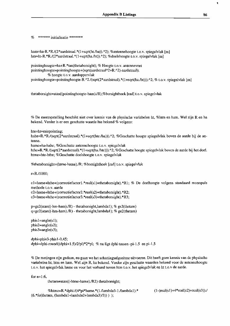
Appendix B Listings
% ****** initialisatie *******
ham=ha-R.*R./(2*aardstraal.*(1+sqrt(ht./ha)).Jl2); %antennehoogte t.o.v. spiegelvlak [m]hm=ht-R.*R./(2*aardstraal.*(1+sqrt(ha./ht)).Jl2); %doelshoogte t.o.v. spiegelvlak [m]
pointinghoogte=ha+R.*tan(thetaborsight); % Hoogte t.o.v. antennevoetpointinghoogte=pointinghoogte+(sqrt(aardstraaIJl2+R.Jl2)-aardstraal);
% hoogte t.o.v. aardoppervlakpointinghoogte=pointinghoogte-R.Jl2.I(sqrt(2*aardstraal).*(1+sqrt(ha./ht))).Jl2; % t.o.v. spiegelvlak [m]
thetaborsight=atan((pointinghoogte-ham)./R);%borsighthoek [rad] t.o.v. spiegelvlak
86
% De meetopstelling beschikt niet over kennis van de physische variabelen ht, %htm en ham. WeI zijn R en habekend. Verder is er een geschatte waarde hte bekend % volgens:
hte=ht+mispointing;hahe=R.*R./(sqrt(2*aardstraal).*(1+sqrt(hte./ha))).Jl2; %Geschatte hoogte spiegelvlak boven de aarde bij de antenne.hame=ha-hahe; %Geschatte antennehoogte t.o.v. spiegelvlakhthe=R.*R./(sqrt(2*aardstraal).*(1+sqrt(ha./hte))).Jl2; %Geschatte hoogte spiegelvlak boven de aarde bij het doel.htme=hte-hthe; %Geschatte doelshoogte t.o.v. spiegelvlak
%thetaborsight=(htme-hame)./R; %borsighthoek [rad] t.o.v. spiegelvlak
r=R./lOOO;
c l=hame+hthe+(correctiefactorl.*real(s1)+thetaborsight).*Rl; % De doelhoogte volgens standaard monopulsmethode t.o.v. aardec2=hame+hthe+(correctiefactor2.*real(s2)+thetaborsight).*R2;c3=hame+hthe+(correctiefactor3.*real(s3)+thetaborsight).*R3;
p=gs2(atan«-hm-ham)./R) - thetaborsight,lambdal); % gs2(thetam)q=ge2(atan«-hm-ham)./R) - thetaborsight,lambdal); % ge2(thetam)
phis1=angle(s 1);phis2=angle(s2);phis3=angle(s3);
dphi=phis3-phis 1-0.45;dphi=dphi-round«dphi+1.5)/2/pi)*2*pi; % nu ligt dphi tussen -pi-1.5 en pi-1.5
% De metingen zijn gedaan, nu gaan we het schattingsalgoritme uitvoeren. Dit heeft geen kennis van de physischevariabelen ht, htm en ham. WeI zijn R, ha bekend. Verder zijn geschatte waarden bekend voor de antennehoogtet.o.v. het spiegelvlak hame en voor het verband tussen htm t.o.v. het spiegelvlak en ht t.o.v de aarde.
for n=I:6,thetam=atan((-htme-hame).00)-thetaborsight;
%htme=R.*dphi./(4*pi*hame.*( l.flambda3-1.flambda1).*(6.*fe(thetam, (lambda1+lambda2+lambda3)/3))) );
(l-(real(s 1)+4*real(s2)+real(s3))./

,
87 Target height estimation in multipath using monopulse complex angle
A 1=(1-1 *real(s1)./fe(thetam,lambdal )).*4.*pi.*hame./(R1.*lambdal ).1\2;A2=(1-1 *real(s2)./fe(thetam,lambda2)).*4.*pi.*hame./(R2.*lambda2).1\2;A3=(1-1 *real(s3)./fe(thetam,lambda3)).*4.*pi.*hame./(R3.*lambda3).1\2;
htme=dphi./integrate(R1.*lambdal ,R2.*lambda2,R3.*lambda3,Al ,A2,A3);%htme=dphi./(Al +4*A2+A3).*6.1(R3.*lambda3-Rl.*lambda1);%htme=dphi./(Al +A3).*2./(R3.*lambda3-Rl.*lambdal);
%htme=R.*dphi./( 4*pi*hame*( Illambda3-1llambda I).*( l-(real(s I)+real(s3))./(2.*fe(thetam,(lambdal+lambda3)12))) );
sr=(s I+4*s2+s3)/6;%htme=R.*(s3-s1)./( 4*pi*hame*( Illambda3-1llambdal).*(j *sr-j*sr.*sr./fe(thetam,
(lambdal+lambda2+lambda3)/3)) );%htme=R.*(real(s3)-real(s1))./(4*pi*hame*( Illambda3-1llambda1).*(-imag(sr)+2*real(sr).*imag(sr)./
fe(thetam, (lambda1+lambda2+lambda3)/3)) );end;
% ********* En tenslotte plotten we het resultaat
d=real(htme)+hthe; % gemeten doelshoogte t.o.v. aardee=d-ht;d(LOW)=-IO; % maak laatste verste hoogte nul, i.v.m. met net plaatjee(LOW)=-IO;c2(LOW)=-1O;
m=fe(thetam,lambda2);gamma= real(s2)./abs(s2).1\2 - 2./fe(thetam,lambda2) + real(s2).Ife(thetam,lambda2).1\2;dht=hm.*gamma./( R.*correctiefactor2.*(1-real(s2)./m)); % mispointing criterium.
dht(LOW)=-lO;ht(LOW)=O;ht(LOW-l)=O;
subplot(4,1,1 );grid; hold;plot(r,min(80,max(-1 0,c2)));ylabel('ht monopulse [m]');xlabel('Rt [km]');plot(r,min(80,max(-1O,ht)),'r');
subplot(4,1 ,2);grid; hold;plot(r,-dphi);ylabel('-dphis [rad]');xlabel('Rt [km]');
subplot(4,1 ,3);grid; hold;plot(r,min(80,max(-1O,d)));ylabel('ht complex angle [m]');xlabel('Rt [km]');plot(r,min(80,max(-1 O,ht)),'r');
subplot(4,1 ,4);grid; hold;plot(r,min(5,max(-5,dht)));plot(r,I);ylabel('mispointing criterium');xlabel('Rt [km]');subplot(4,1,1);