EG Slope Stability - Geoplanning · · 2012-02-13Geologic Conditions Potential Failure Surface...

ENVIRONMENTAL GEOTECHNICS

NATURAL AND ARTIFICIAL SLOPES andGENERAL SLOPE STABILITY CONCEPTS

Prof. Ing. Marco Favarettig

Università di Padova Facoltà di Ingegneria

Dipartimento di Ingegneria Idraulica, Marittima, Ambientale e Geotecnica (I.M.A.GE.)

Via Ognissanti, 39 – 35129 – Italia

Tel: +39.049.827.7901 Fax: +39.049.827.7988

E‐Mail: [email protected]@ p

1

fi i i fDefinition of LANDSLIDE

The downward falling or sliding of a mass of soil, detritus, or rock on or

from a steep slope.

Introduction to SLOPE STABILITY

Slope stability problems have been faced throughout history when men

and women or nature has disrupted the delicate balance of natural soilp

slopes.

N d t d t d l ti l th d i ti ti t l dNeed to understand analytical methods, investigative tools, and

stabilization methods to solve slope stability problems.

2

AIMS OF SLOPE STABILITY ANALYSIS

The primary purpose of slope stability analysis is to contribute to the safe

and economic design of excavations embankments earth dams landfillsand economic design of excavations, embankments, earth dams, landfills,

and spoil heaps.

The aims of slope stability analyses are:

(1) To understand the development and form of natural slopes and the

processes responsible for different natural features.processes responsible for different natural features.

(2) To assess the stability of slopes under short-term (often during( ) y p ( g

construction) and long-term conditions.

3

AIMS OF SLOPE STABILITY ANALYSIS

(3) To assess the possibility of landslides involving natural or existing

i d lengineered slopes.

(4) To analyze landslides and to understand failure mechanisms and the(4) To analyze landslides and to understand failure mechanisms and the

influence of environmental factors.

(5) To enable the redesign of failed slopes and the planning and design of

preventive and remedial measures, where necessary.preventive and remedial measures, where necessary.

(6) To study the effect of seismic loadings on slopes and embankments.( ) y g p

4

NATURAL AND ARTIFICIALS SLOPES

The analysis of slopes takes into account a variety of factors relating to

topography, geology, and material properties, often relating to whether the

slope was naturally formed or engineered.

Natural slopes that have been stable for many years may suddenly fail

b f h i t h i i it d t fl l fbecause of changes in topography, seismicity, groundwater flows, loss of

strength, stress changes, and weathering.

Significant uncertainty exists about the stability of a natural slopeSignificant uncertainty exists about the stability of a natural slope.

5

NATURAL AND ARTIFICIALS SLOPES

Knowing that old slip surfaces exist in a natural slope makes it easier to

understand and predict the slope’s behavior. The shearing strength along

these slip surfaces is often very low because prior movement has caused

slide resistance to peak and gradually reduce to residual values.

Engineered slopes may be considered in three main categories:

embankments, cut slopes, and retaining walls. As these slopes are man-

made less uncertainty exists about their stability.

6

MODES OF FAILURE

Slope failures are usually due either to a sudden or gradual loss of

strength by the soil or to a change in geometric conditions, for

example, steepening of an existing slope.

7

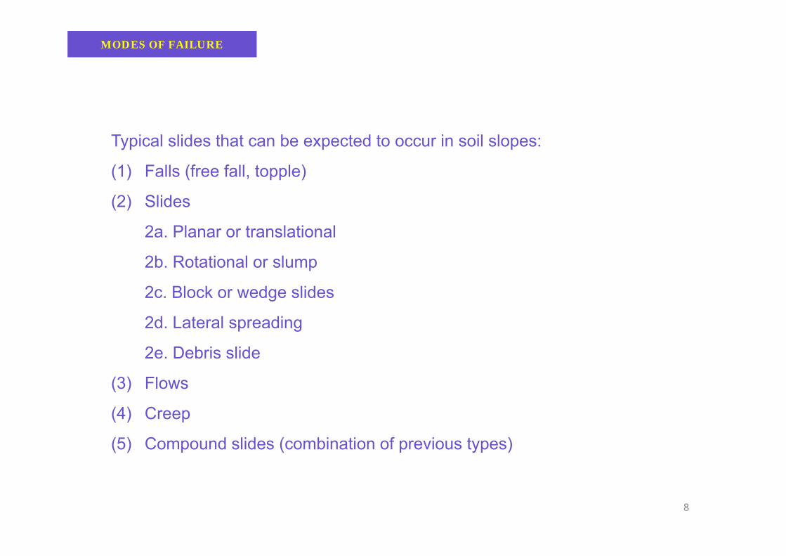
MODES OF FAILURE

Typical slides that can be expected to occur in soil slopes:

(1) Falls (free fall, topple)

(2) Slides

2a. Planar or translational

2b. Rotational or slump

2c. Block or wedge slides

2d. Lateral spreading

2e. Debris slide

(3) Flows

(4) Creep

(5) Compound slides (combination of previous types)

8

MODES OF FAILURE

9

Falls

Free fall

Topple

10

Slides

Rotational Slide

Usually occurs in

slopes consisting of

homogeneous

materials

Translational Slide

Usually occurs in

shallow soils

overlying relativelyoverlying relatively

stronger materials

11

Lateral spreading & Debris flow

Lateral spreading

Debris flow

12

MODES OF FAILURE

As most soils are generally heterogeneous, noncircular surfaces,

consisting of a combination of planar and curved sections, are most likely.

Often retrogressive failuresOften, retrogressive failures

consisting of multiple curved

surfaces can occur in layeredsurfaces can occur in layered

soils. Such failures are typical

where the first slip tends towhere the first slip tends to

oversteepen the slope, which

then leads to additional failures.

Such failures are typical where the first slip tends to oversteepen the

slope, which then leads to additional failures.

13

MODES OF FAILURE

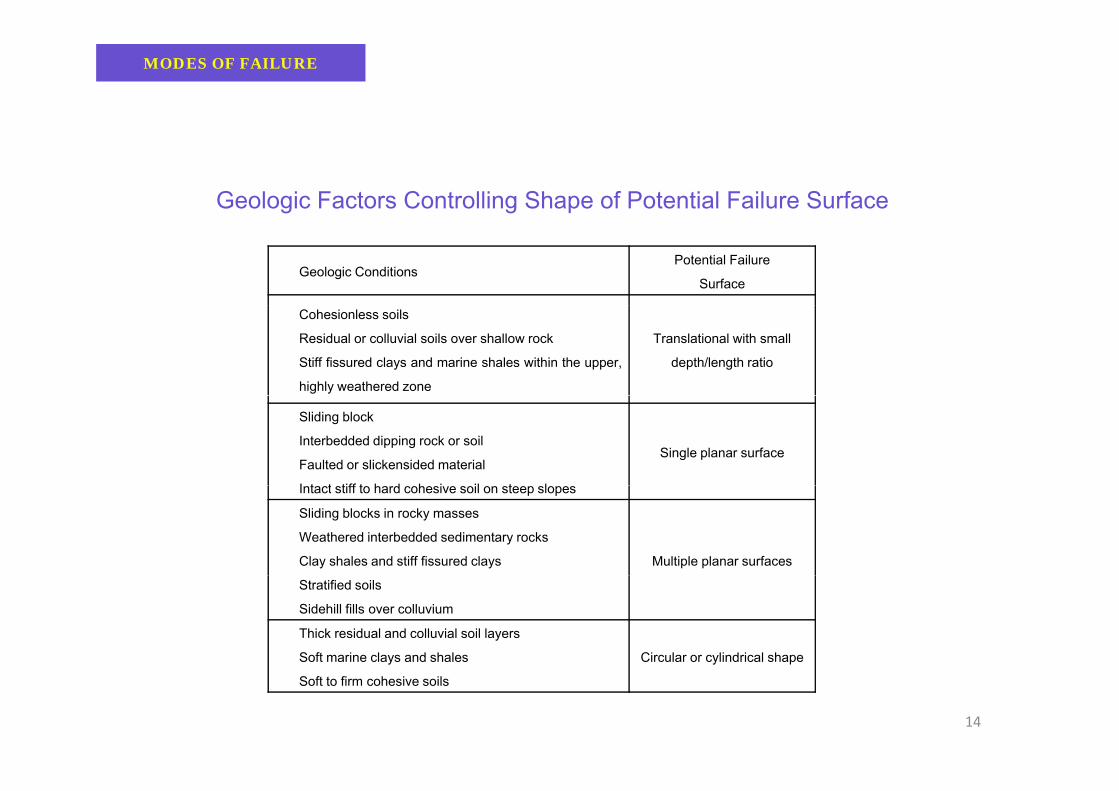
Geologic Factors Controlling Shape of Potential Failure Surface

Geologic ConditionsPotential Failure

Surface

Cohesionless soils

Residual or colluvial soils over shallow rock

Stiff fissured clays and marine shales within the upper,

highly weathered zone

Translational with small

depth/length ratio

Sliding block

Interbedded dipping rock or soil

Faulted or slickensided material

I t t tiff t h d h i il t l

Single planar surface

Intact stiff to hard cohesive soil on steep slopes

Sliding blocks in rocky masses

Weathered interbedded sedimentary rocks

Clay shales and stiff fissured clays Multiple planar surfaces

Stratified soils

Sidehill fills over colluvium

Thick residual and colluvial soil layers

Soft marine clays and shales Circular or cylindrical shape

Soft to firm cohesive soils

14

CASE HISTORIES (1)

Toppling failure

Planar Sliding

15

CASE HISTORIES (2)

Lateral spreading

T ll V ll L d lidTully Valley Landslide,

Phoenix, New York, 199316

CASE HISTORIES (3)

C f d j i dCones of dejection and screes at

the feet of Canadian Rockies

17

CASE HISTORIES (4)

S. Salvador, El Salvador, 2001

Debris Flow18

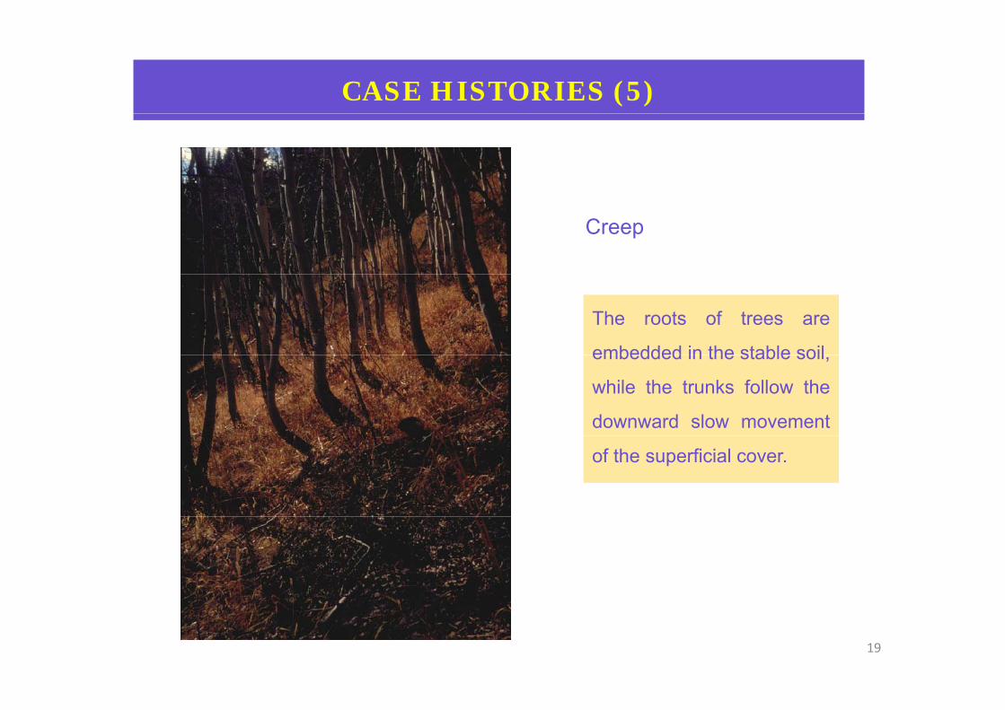
CASE HISTORIES (5)

Creep

The roots of trees are

embedded in the stable soilembedded in the stable soil,

while the trunks follow the

downward slow movement

of the superficial cover.

19

CASE HISTORIES (6)

Rotational landslide

with debris-flow

La Conchita, California, 1995

20

CASE HISTORIES (7)

F S J h AlbFort St. John, Alberta,

Canada, 2001

Roto-traslational

l d lidlandslide

Young River Landslide, Canada

21

FACTORS INFLUENCING SLOPE STABILITY

The main items required to evaluate the stability of a slope are:q y p

(1) Shear strength of the soils

(2) Slope geometry( ) p g y

(3) Pore pressures or seepage forces

(4) Loading and environmental conditions

(1) The shear strengths should be provided as undrained strength, su, or

th t i l M h C l b t d φthe more typical Mohr-Coulomb parameters, c and φ.

(2) The slope geometry may be known for existing, natural slopes or may

be a design parameter for embankments and cut slopesbe a design parameter for embankments and cut slopes.

(3) A major contributor to many slope failures is the change in effective

stress caused by pore water pressures These tend to alter the shearstress caused by pore water pressures. These tend to alter the shear

strength of the soil along the shear zone22

( )FACTOR OF SAFETY (FOS) CONCEPTS

F ti f th FOS t t f t i t d th t d i tFunction of the FOS: to account for uncertainty, and thus to guard against

ignorance about the reliability of the items that enter into the analysis,

such as strength parameters pore pressure distribution and stratigraphysuch as, strength parameters, pore pressure distribution, and stratigraphy.

The lower the quality of the site investigation, the higher the desired FOS

should be.

The FOS used in design will vary with material type and performance

requirements.

The required FOSs (nonseismic) are usually in the 1.25 to 1.5 range.

Higher factors may be required if there is a high risk of loss of life or

uncertainty regarding the pertinent design parameters. Likewise, lower

FOS b d if h i i fid f h f iFOSs may be used if the engineer is confident of the accuracy of input

data and if the construction is being monitored closely. 23

i fi i iFACTOR OF SAFETY– First Definition

In most limit equilibrium analyses, the shear strength required along a

potential failure surface to just maintain stability is calculated and thenp j y

compared to the magnitude of available shear strength. In this case the

FOS is assumed to be constant for the entire failure surface.

This average FOS will be given by the ratio of available to required shear

strength:

for total stressessu

req =τ for total stresses

for effective stresses

Freqτ

φ⋅σ+=τ

tan''c

24φ

+=τFFc

req

i fi i iFACTOR OF SAFETY– First Definition

The adoption of Fc and Fφ allows different proportions of the cohesive (c’)

and frictional (φ‘) components of strength to be mobilized along the failure(φ ) p g g

surface.

However, most limit equilibrium methods assume Fc and Fφ , implying that

the same proportion of the c’ and φ‘ components are mobilized at thep p φ p

same time along the shear failure surface.

25

d fi i iFACTOR OF SAFETY– Second Definition

Another definition of FOS often considered is the ratio of total resisting

forces to total disturbing (or driving) forces for planar failure surfaces org ( g) p

the ratio of total resisting to disturbing moments, as in the case for circular

slip surfaces.

Realize that these different values of the FOS obtained using the three

methods, that is, mobilized strength, ratio of forces, or ratio of moments, will

not give identical values for c – φ soils.

26

FACTOR OF SAFETY

First definitionFirst definition

Second definition

27

PORE WATER PRESSURES

If ff ti t l i i t b f d t illIf an effective stress analysis is to be performed, pore water pressures will

have to be estimated at relevant locations in the slope. These pore

pressures are usually estimated from groundwater conditions that may bepressures are usually estimated from groundwater conditions that may be

specified by one of the following methods:

(1) Phreatic Surface: This surface, or line in two dimensions, is defined by

the free groundwater level. Delineated, in the field, by using open

standpipes as monitoring wells.

(2) Piezometric Data: Specification of pore pressures at discrete points,

ithi th l d f i t l ti h t ti t thwithin the slope, and use of an interpolation scheme to estimate the

required pore water pressures at any location. Determined from field

piezometers a manually prepared flow net or a numerical solution usingpiezometers, a manually prepared flow net or a numerical solution using

finite differences or finite elements. 28

PORE WATER PRESSURES - ru

(3) P W t P R ti Thi i l d i l th d f(3) Pore Water Pressure Ratio: This is a popular and simple method for

normalizing pore water pressures measured in a slope according to the

definition:definition:

vu

urσ

=

where u is the pore pressure and σv, is the total vertical subsurface soil

stress at depth z Effectively the r value is the ratio between the pore

v

stress at depth z. Effectively, the ru, value is the ratio between the pore

pressure and the total vertical stress at the same depth.

This factor is easily implemented but the major difficulty is associated withThis factor is easily implemented, but the major difficulty is associated with

the assignment of the parameter to different parts of the slope.

It is usually reserved for estimating the FOS value from slope stabilityIt is usually reserved for estimating the FOS value from slope stability

charts or for assessing the stability of a single surface.29

PORE WATER PRESSURES

(4) Pi t i S f Thi f i d fi d f th l i f(4) Piezometric Surface: This surface is defined for the analysis of a

unique, single failure surface. This approach is often used for the back

analysis of failed slopesanalysis of failed slopes.

Note that a piezometric surface is not the same as a phreatic surface asNote that a piezometric surface is not the same as a phreatic surface, as

the calculated pore water pressures will be different for the two cases.

(5) Constant Pore Water Pressure: This approach may be used if the

i i h t if t t t i ti lengineer wishes to specify a constant pore water pressure in any particular

soil layer.

30

h i fPORE WATER PRESSURES – Phreatic surface

If h ti f i d fi d th t l l t d fIf a phreatic surface is defined, the pore water pressures are calculated for

the steady-state seepage conditions.

Thi t i b d th ti th t ll i t ti l liThis concept is based on the assumption that all equipotential lines are

straight and perpendicular to the segment of the phreatic surface passing

through a slice element in the slopethrough a slice-element in the slope.

31

h i fPORE WATER PRESSURES – Phreatic surface

Th if th i li ti f th h ti f t i θ d th ti lThus if the inclination of the phreatic surface segment is θ, and the vertical

distance between the base of the slice and the phreatic surface is h, the

pore pressure is given by:pore pressure is given by: ( )θ⋅⋅γ= 2ww coshu

This is a reasonable assumption for a

sloping straight-line phreatic surface, butp g g p ,

will provide higher or lower estimates of

pore water pressure for a curved

(convex) phreatic surface.

32

i i fPORE WATER PRESSURES – Piezometric surface

N t th t th ti l di t ( l ti l h d) i t k t t thNote that the vertical distance (elevational head) is taken to represent the

pressure.

There are some computer programs that oversimplify the analysis by

i i t ti h ti f i t i f With thimisinterpreting a phreatic surface as a piezometric surface. With this

erroneous assumption, the overestimated pore pressure head is incorrectly

taken as the vertical distance between the phreatic surface and base oftaken as the vertical distance between the phreatic surface and base of

slice.33

i

Th b h i i h t ti

Negative Pore Pressures

There may be cases where an engineer wishes to use negative pore

pressures to take advantage of the apparent cohesive strength available

due to suction within the soil in the slopedue to suction within the soil in the slope.

The influence of suction should be included by increasing the total cohesion

according to the measured values of matric suction within the slopeaccording to the measured values of matric suction within the slope.

In some cases, actual negative pore pressures have been used in slope

analysis to increase the shear strength of the soilanalysis to increase the shear strength of the soil.

This method is not recommended, as it only affects the frictional component

via the (σ – u) tan φ term and may not generate reliable values of strength.via the (σ u) tan φ term and may not generate reliable values of strength.

34

LIMIT EQUILIBRIUM METHOD – L.E.M.

There are numerous methods currently available for performing slope

stability analyses. The majority of these may be categorized as limit

equilibrium methods.

All the procedures currently used are based on the L.E.M. and have the

following assumptions in common:following assumptions in common:

• Coulomb’s failure criterion is satisfied along the assumed failure

surface, which may be a straight line, circular arc, logarithmic spiral, or, y g , , g p ,

other irregular surface.

• Plain strain conditions are supposed.

• The actual strength of the soil is compared with the value required for

the equilibrium of the soil mass and this ratio is a measure of the safety

factor.35

I thi th d il t t d i id l ti t i l d d t thi


In this method soils are treated as rigid-plastic materials and due to this

assumption the analysis does not consider deformations. Therefore, this

method allows to only condition at the onset of failuremethod allows to only condition at the onset of failure.

These methods are very similar to the kinematic approach, but frequently

the restrictions of a kinematically admissible mechanisms are ignored.

Limit Equilibrium Methods can be subdivided in two principal categories:Limit Equilibrium Methods can be subdivided in two principal categories:

• Methods that consider only the whole free body (Culmann method,

friction circle method)friction circle method).

• Methods that divide the free body into many vertical slices and consider

equilibrium of each slide (method of slices).equilibrium of each slide (method of slices).

36


37

Th t i l t l l t bilit

INFINITE SLOPE ANALYSIS

The most simple way to analyze slope stability.

It is used when:

• A slope extends for a relatively long distance and has a consistent• A slope extends for a relatively long distance and has a consistent

subsoil profile.

The failure plane is parallel to the surface of the slope and the limit

equilibrium method can be applied readily.

.Infinite slopes can be studied under several configurations:

• Infinite slope in dry sand• Infinite slope in dry sand.

• Infinite slope in c – φ soil with seepage: seepage parallel to the slope.

• Infinite slope in c – φ soil with seepage: horizontal seepage (i.e. rapidInfinite slope in c φ soil with seepage: horizontal seepage (i.e. rapid

dewatering of canals).38

ilINFINITE SLOPE ANALYSIS – Dry Soil

I t li t i th

Dry Soil

Interslice tensions on the

lateral sides of each element

are equal so the soil massare equal, so the soil mass

moves like a continuum.

Th l (W ) d d i i (W )The normal (W┴) and driving (W//)

forces are determined:

W┴ = W cosβ = γ b h 1 cosβ

W// = W sinβ = γ b h 1 sinβ where β is the constant inclination of the slope

39

ilINFINITE SLOPE ANALYSIS – Dry Soil

The available frictional strength along the failure plane will depend on φ

and is given by

If we consider the FOS as the ratio of available strength to strength

S = c’ b secβ + N tan φ = c’ b secβ + W┴ tan φ

required to maintain stability (limit equilibrium), the FOS will be given by

φ⋅β⋅+β⋅⋅φ⋅+β⋅⋅ 'tancosWsecb'c'tanNsecb'cSFOS

If we assume c’ = 0, FOS will be:

β⋅φββ

=β⋅

φβ==

sinWsinWWFOS

//

,

φ=

tanFOS

40

βtanOS

il i hINFINITE SLOPE ANALYSIS – Soil with seepage

If t t d l i h i φ

Seepage parallel to the slope

If a saturated slope, in cohesive c - φ

soil, has seepage parallel to the

slope surface the same limitslope surface the same limit

equilibrium concepts may be applied

to determine the FOS which willto determine the FOS, which will

now depend on the effective normal

force (N’)force (N ).

The total and effective weight of the slice, in this case, are respectively

given by:given by:

W = γsat b h 1 and W’ = (γsat - γw) b h 1 = γ’ b h 1 41


The effective normal force N’ is given by: N’ = N – U

where N is the total normal force and U the pore water force acting on the

base of the slice:

N = W┴ = W cosβ = γsat b h cosβ

( ) β⋅⋅⋅γ=β

⋅β⋅⋅γ= coshbcos

bcoshU w2

w

So the effective normal force N’ is given by:

N’ = (γsat - γw) b h 1 cosβ = γ’ b h 1 cosβ

The driving forces can be given by:

W’// = W’ sinβ = γ’ b h 1 sinβ

Pw = pw V = γw i V = γw i b h 1 42


where Pw is the seepage force and i is the hydraulic gradient defined as the

ratio between the hydraulic head measurements over the length of the flow

path:β=

ββ⋅

=Δ

= sincos/btanb

Lhi

So Pw will be given by:

Pw = γw i b h 1 = γw b h 1 sinβ

The available frictional strength along the failure plane will depend on φ’

and the effective normal force and is given byg y

S = c’ b secβ + (N – U) tan φ’

= c’ b secβ + N’ tan φ’ = c’ b secβ + γ’ b h 1 cosβ tan φ’

43

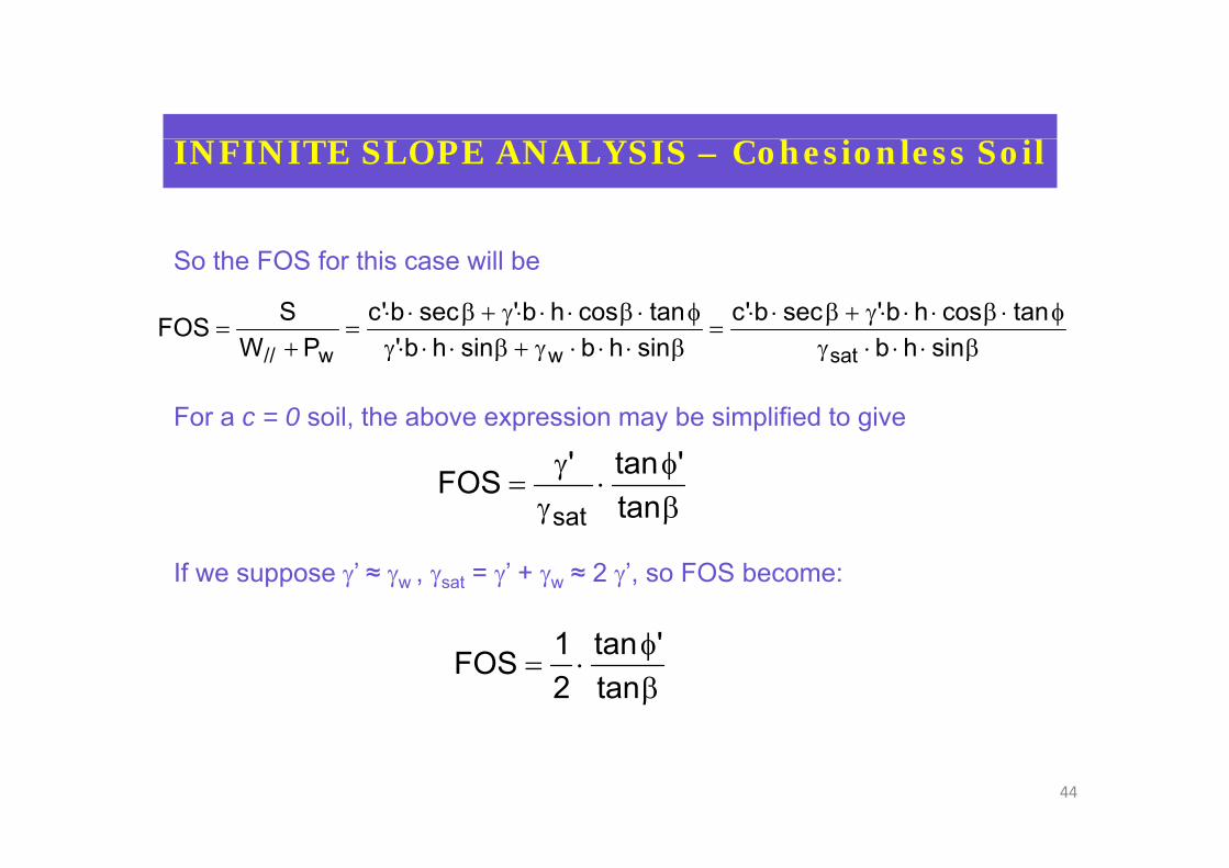
h i l ilINFINITE SLOPE ANALYSIS – Cohesionless Soil

So the FOS for this case will be

φ⋅β⋅⋅⋅γ+β⋅⋅=

φ⋅β⋅⋅⋅γ+β⋅⋅==

tancoshb'secb'ctancoshb'secb'cSFOS

For a c = 0 soil, the above expression may be simplified to give

β⋅⋅⋅γβ⋅⋅⋅γ+β⋅⋅⋅γ+ sinhbsinhbsinhb'PWFOS

satww//

βφ

⋅γ

γ=

tan'tan'FOS

sat

If we suppose γ’ ≈ γw , γsat = γ’ + γw ≈ 2 γ’, so FOS become:

βφ

⋅=tan

'tan21FOS

44


Horizontal Seepage

Th t t l d ff ti i ht f thThe total and effective weight of the

slice, also in this case, are

respectively given by:respectively given by:

W = γsat b h 1

W’ = (γsat - γw) b h 1 = γ’ b h 1

The effective normal force N’ is given by: N’ = N – U cosβ

where N is the total normal force and U the pore water force acting on the

base of the slice:

N = W┴ = W cosβ = γsat b h cosβ and U = γw b h45


So the effective normal force N’ is given by:

N’ = (γsat - γw) b h 1 cosβ = γ’ b h 1 cosβ

The driving forces can be given by:

W’// = W’ sinβ = γ’ b h 1 sinβ

Pw = pw V = γw i V = γw i b h 1

where P is the seepage force and i is the hydraulic gradient defined as thewhere Pw is the seepage force and i is the hydraulic gradient defined as the

ratio between the hydraulic head measurements over the length of the flow

path that in this case is given by:path, that, in this case, is given by:

β=β⋅

=Δ

= tanbtanb

Lhi

46

bL


So Pw will be given by:

Pw = γw i b h 1 = γw b h 1 tanβ

In this seepage condition, Pw lies on horizontal direction, so we can

subdivide Pw in the perpendicular and parallel components:

Pw,┴ = Pw sinβ = γw b h 1 tanβ sinβ

Pw,// = Pw cosβ = γw b h 1 tanβ cosβ

The available frictional strength along the failure plane will depend on φ’,

the effective normal force N’ and Pw ┴ and is given byw, g y

S = c’ b secβ + (N’ - Pw,┴) tan φ’

= c’ b secβ + (γ’ b h 1 cosβ − γw b h 1 tanβ sinβ) tan φ’w

47

h i l ilINFINITE SLOPE ANALYSIS – Cohesionless Soil

Then, the FOS for this case will be

If we suppose c’ = 0 and γ’ ≈ γw FOS become:

48

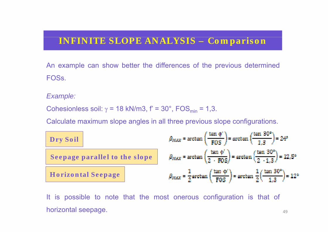
iINFINITE SLOPE ANALYSIS – Comparison

A l h b tt th diff f th i d t i dAn example can show better the differences of the previous determined

FOSs.

Example:

Cohesionless soil: γ = 18 kN/m3, f’ = 30°, FOSmin = 1,3.

Calculate maximum slope angles in all three previous slope configurations.

Dry Soily

Seepage parallel to the slope

Horizontal Seepage

It i ibl t t th t th t fi ti i th t fIt is possible to note that the most onerous configuration is that of

horizontal seepage. 49

CIRCULAR SURFACE ANALYSIS

Ci l f il f f d t b th t iti l i lCircular failure surfaces are found to be the most critical in slopes

consisting of homogeneous materials.

There are two analytical methods that may be used to calculate the FOS

for a slope :for a slope :

• the circular arc (φ = 0)the circular arc (φ 0)

• Friction circle.Friction circle.

50

i lCIRCULAR SURFACE ANALYSIS – Circular Arc

Th i l t i l l i i b d th ti th t i idThe simplest circular analysis is based on the assumption that a rigid,

cylindrical block will fail by rotation about its center and that the shear

strength along the failure surface is defined by the undrained strengthstrength along the failure surface is defined by the undrained strength.

As the undrained strength is

d th l f i t lused, the angle of internal

friction, φ, is assumed to be

zero (hence the φ = 0 method )zero (hence the φ = 0 method )

The FOS for such a slope may

b l d b t ki th tibe analyzed by taking the ratio

of the resisting and overturning

moments about the center ofmoments about the center of

the circular surface O.51

i lCIRCULAR SURFACE ANALYSIS – Circular Arc

If th t i t i b W d i ti tIf the overturning moments are given by W1x1 and resisting moments are

given by cuLR + W2x2, the factor of safety for the slope will be:

If the undrained shear strengthIf the undrained shear strength

varies along the failure

surface the c L term must besurface, the cuL term must be

modified and treated as a

variable in the abovevariable in the above

formulation.

52

i i i lCIRCULAR SURFACE ANALYSIS – Friction Circle

Thi th d i f l f h il ith φ 0 h th t thThis method is useful for homogeneous soils with φ > 0, such that the

shear strength depends on the normal stress.

It may be used when both cohesive and frictional components for shearIt may be used when both cohesive and frictional components for shear

strength have to be considered in the calculations.

The method is equally suitable for total or effective stress types of analysisThe method is equally suitable for total or effective stress types of analysis.

The method attempts to satisfy the requirement of complete equilibrium by

i th di ti f th lt t f th l d f i ti lassuming the direction of the resultant of the normal and frictional

component of strength mobilized along the failure surface. This direction

corresponds to a line that forms a tangent to the friction circle with acorresponds to a line that forms a tangent to the friction circle, with a

radius, Rf = R sin φm.

This assumption is guaranteed to give a lower bound FOS value.53


Th h i h t l th b f th f il f b illThe cohesive shear stresses along the base of the failure surface ab, will

have a resultant, Cm, that acts parallel to the direction of the chord ab.

Its location may be found by taking moments of the distribution and theIts location may be found by taking moments of the distribution and the

resultant, Cm, about the circle center. This line of action of resultant, Cm,

can be located usingcan be located using

The distance Rc of this line from

th t f th i l O ithe center of the circle O is:

54


Th t l i t f li ti A i l t d t th i t ti f thThe actual point of application, A, is located at the intersection of the

effective weight force, which is the resultant of the weight and any pore

water forces The resultant of the normal and frictional (shear) force P willwater forces. The resultant of the normal and frictional (shear) force, P, will

then be inclined parallel to a line formed by a point of tangency to the

friction circle and point Afriction circle and point A.

As the direction of Cm is known,

the force polygon can be closedthe force polygon can be closed

to obtain the value of the

mobilized cohesive force. Again,mobilized cohesive force. Again,

the final FOS is computed with

the assumption Fφ = Fc = FOSp φ c

along the failure circular surface.55


Th l ti d i ll f ll d hi ll S l ti dThe solution procedure is usually followed graphically. Solution procedure:

(1) Calculate weight of slide, W.

(2) Calculate magnitude and direction of the resultant pore water force, U

(may need to discretize slide into slices).

(3) C l l di l di(3) Calculate perpendicular distance

to the line of action of Cm.

(4) Fi d ff ti i ht lt t(4) Find effective weight resultant,

W ’, from forces W and U, and its

intersection with the line of actionintersection with the line of action

of Cm at A.

(5) Assume a value of Fφ(5) Assume a value of Fφ.

(6) Calculate the mobilized friction angle φm = tan-1 (tan φ) / Fφ .56

i i i l

(7) D th f i ti i l ith di R R i φ

CIRCULAR SURFACE ANALYSIS – Friction Circle

(7) Draw the friction circle, with radius Rf = R sin φm.

(8) Draw the force polygon with W ’ appropriately inclined, and passing

through point Athrough point A.

(9) Draw the direction of P, tangential to the friction circle.

(10) Draw direction of C according(10) Draw direction of Cm, according

to the inclination of the chord linking

the end-points of the failure surfacethe end points of the failure surface.

(11) The closed polygon will then

provide the value of Cm.provide the value of Cm.

(12) Using this value of Cm, calculate

Fc = c Lchord / Cm.c chord m

(13) Repeat steps 5 to 12 until Fc ≈ Fφ .57

If th bili d t th f φ il i t b l l t d th di t ib ti

METHOD OF SLICES

If the mobilized strength for a c – φ soil is to be calculated, the distribution

of the effective normal stresses along the failure surface must be known.

This condition is usually analyzed by discretizing the mass of the failureThis condition is usually analyzed by discretizing the mass of the failure

slope into smaller slices and treating each individual slice as a unique

sliding blocksliding block.

The method of slices is used

by most computer programsby most computer programs,

as it can readily accommodate

complex slope geometries,complex slope geometries,

variable soil conditions, and

the influence of external

boundary loads.58

i i ( )

Th l f l ti f th th d f li i l ti t th

METHOD OF SLICES – Basic assumptions (1)

There are several formulations of the method of slices in relation to the

assumption that the numerous authors had made. We can subdivide them

in three categories:in three categories:

1. Assumptions on interslice forces direction

(Bishop, 1955; Spencer, 1967; Morgenstern-Price, 1965)

2 Assumptions on the thrust line position (Janbu 1954)2. Assumptions on the thrust line position (Janbu, 1954)

3. Assumptions on the interslice forces distribution

(Sarma, 1973; Correia, 1988)

59

i i ( )

All th th d b d i il t b t th i diff t

METHOD OF SLICES – Basic assumptions (2)

All these methods are based on similar concepts, but they give different

FOSs values through the previous assumptions. However, all of them are

based on the Mohr Coulomb failure criterion (rigid perfect plastic behavior)based on the Mohr-Coulomb failure criterion (rigid-perfect plastic behavior).

All limit equilibrium methods for slope stability analysis divide a slide massAll limit equilibrium methods for slope stability analysis divide a slide mass

into n smaller slices, so that we can approximate the irregular base of the

slice (often an arc) as a chordslice (often an arc) as a chord.

Another hypothesis is that FOS is considered constant along the failureAnother hypothesis is that FOS is considered constant along the failure

surface.

60

f f

E h li i ff t d b l t f f

METHOD OF SLICES – System of forces

Each slice is affected by a general system of forces.

The thrust line connects theThe thrust line connects the

points of application of the

interslice forcesinterslice forces.

The location of this thruste ocat o o t s t ust

line may be assumed or its

location may be determinedy

using a rigorous method of

analysis that satisfies

complete equilibrium.61

f f

Th l i lifi d th d f l i l t th l ti f th

METHOD OF SLICES – System of forces

The popular simplified methods of analysis neglect the location of the

interslice force because

complete equilibrium is notcomplete equilibrium is not

satisfied for the failure mass.

For this system, there are

(6n – 2) unknowns. Also,

since only four equations for

each slice (4n equations)

can be written for the limit

equilibrium for the system,

the solution is statically

indeterminate. 62

f fMETHOD OF SLICES – System of forces

63

i ( )

A l ti i ibl idi th b f k b d d

METHOD OF SLICES – Assumptions (3)

A solution is possible providing the number of unknowns can be reduced

by making some simplifying assumptions.

One of these common assumptions is that the normal forces on the base

of the slices acts at the midpoint thus reducing the number of unknowns toof the slices acts at the midpoint, thus reducing the number of unknowns to

(5n – 2).

This then requires an additional (n – 2) assumptions to make the problem

determinate.determinate.

It is these assumptions that generally categorize the available methods ofp g y g

analysis.64

h dMETHOD OF SLICES – Common Methods

Li t f th th d f l i d th diti f t tiList of the common methods of analysis and the conditions of static

equilibrium that are satisfied in determining the FOS.

65

l f l iMETHOD OF SLICES – General formulation

C id b d f il th i t f lidi th f ABCD F thConsider a body of soil on the point of sliding on the surface ABCD. For the

purpose of analysis, we will divide the whole body of soil abode the surface

of sliding into n elementary slices separated by n 1 vertical boundariesof sliding into n elementary slices, separated by n-1 vertical boundaries.

The choice of vertical

interslice boundaries is

merely a matter of

convenience.

In general, the failure

condition is not satisfied

on these surfaces.66

l f l iMETHOD OF SLICES – General formulation

If th b d i t bl f d t ilib i diti t bIf the body is stable, force and moment equilibrium conditions must be

satisfied for each slice, and also for the whole body.

The failure condition

τf = c’ + (σn – u) tan φ’

must be satisfied everywhere

on the surface ABCDon the surface ABCD.

If Fc = Fφ = F along the failure

f d fisurface, we may define a

factor of safety in the form

67

l f l i

F th li i T [ b ] N [ b ]

METHOD OF SLICES – General formulation

For the slice i: Ti = [τ b secα]i ; Ni = [σn b secα]iThen:

It will be convenient to specify the pore pressure ui on BC in term of the

pore pressure ratio ru equal to [ub/W]i where Wi is the weight of slice i. Then

(1)( )

Vertical forces equilibrium of slice i

[T i + N ] [W ΔX] (2)[T sinα + N cosα]i = [W - ΔX]iwhere

ΔX = X X

(2)

ΔXi = X(i+1) - Xi

68

l f l i

S b tit ti ti (1) i t b (2) bt i


Substituting equation (1) into number (2) we obtain

Rearranging the terms, this yields

(3)(3)

where

Substitute equation (3) into number (1) to give

(4)69

l f l i

T ti l f ilib i f li i


Tangential forces equilibrium of slice i

R i th t thi i ld

(5)

Rearranging the terms, this yields

Substituting Ti with equation (4) we obtain

In considering the equilibrium of the whole soil mass, the internal interslice

forces (E2 to En and X2 to Xn) must vanish. Also if there are no external

forces on the end slices,

E E X X 0E1 = E(n+1) = X1 = X(n+1) = 0

70

l f l i

S th t


So that

(6)

Moment equilibrium of slice i around pivot OMoment equilibrium of slice i around pivot O

Since the moments of all internal forces (Ei, Xi) must also vanish when

considering the whole body,g y,

(7)

71

l f l i

S b tit ti th i f T d N bt i d i l thi b


Substituting the expression for Ti and Ni obtained previously this becomes

(8)(8)

In the case we have circular failure surface, equation (8) become

(9)

72

Th O di M th d f Sli (OMS) thi th d (F ll i 1927 1936)

METHOD OF SLICES – OMS

The Ordinary Method of Slices (OMS): this method (Fellenius, 1927, 1936)

is one of the simplest procedures based on the method of slices and

neglects all interslice forces (X and E ) and fails to satisfy force equilibriumneglects all interslice forces (Xi and Ei) and fails to satisfy force equilibrium

for the slide mass as well as for individual slices. So the number of

unknowns become: (5n 2) (n 1) (n 1) (n 1) = 2n +1 unknownsunknowns become: (5n – 2) – (n – 1) – (n – 1) – (n – 1) = 2n +1 unknowns

< 4n equations.

This method consider a circular failure surface

Xi Ei zi

This method consider a circular failure surface.

If we remember that:

and manipulating equation (7) to give

73

bt i

METHOD OF SLICES – OMS

we obtain

The Ordinary Method of Slices can be used also in the case of layeredThe Ordinary Method of Slices can be used also in the case of layered

soils. It is sufficient to consider the correct soil strength parameter (c’ and

φ’) at the base of each sliceφ ) at the base of each slice.

74

i h ’ h d

Th Bi h ’ M th d i f th t f th d b d li it

METHOD OF SLICES – Bishop’s Method

The Bishop’s Method is one of the most famous methods based on limit

equilibrium. He makes the hypothesis of a circular failure surface.

There are two different approaches:

a. Bishop’s Rigorous Method.

Satisfy moment equilibrium – circular failure surfaceSatisfy moment equilibrium circular failure surface

b. Bishop’s Simplified Method.b. Bishop s Simplified Method.

Satisfy complete equilibrium – circular failure surface

75

i h ’ h d

Bi h ’ Ri M th d


a. Bishop’s Rigorous Method

Bishop (1955) considers in his rigorous formulation equation (6) and

equation (9).

He also imposed that

Xi = λ f(x)

where λ is a constant unknown and f(x) a known function.

We saw early that there are n – 2 additional unknown which make the

bl i d t i t I thi d t th i ti ll Xproblem indeterminate. In this case, due to the previous assumption, all Xi

become known if λ is defined. Therefore, the total number of unknowns is:

(5n 2) (n 1) + 1 4n nkno ns 4n eq ation The problem is(5n – 2) – (n – 1) + 1 = 4n unknowns = 4n equation. The problem is

determinate and the equilibrium equations are satisfied. 76

i h ’ h d

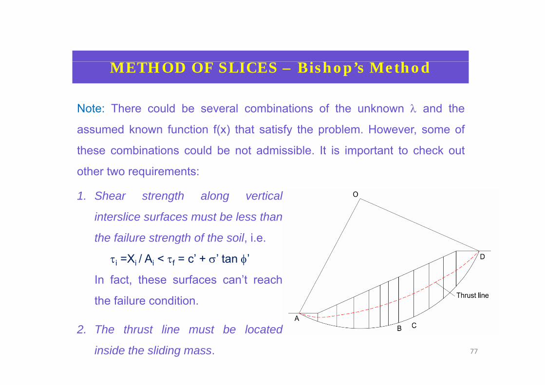
N t Th ld b l bi ti f th k λ d th


Note: There could be several combinations of the unknown λ and the

assumed known function f(x) that satisfy the problem. However, some of

these combinations could be not admissible It is important to check outthese combinations could be not admissible. It is important to check out

other two requirements:

1 Sh t th l ti l1. Shear strength along vertical

interslice surfaces must be less than

the failure strength of the soil i ethe failure strength of the soil, i.e.

τi =Xi / Ai < τf = c’ + σ’ tan φ’

In fact these surfaces can’t reachIn fact, these surfaces can t reach

the failure condition.

2. The thrust line must be located

inside the sliding mass. 77

i h ’ h dMETHOD OF SLICES – Bishop’s Method

b Bi h ’ Si lifi d M th db. Bishop’s Simplified Method

In his simplified approach, Bishop (1955) assumes that all vertical interslice

shear forces Xi are zero, reducing the number of unknowns by (n – 1). This

leaves (4n – 1) unknowns, leaving the solution overdetermined.

So, Xi = 0, λ = 0 and ΔXi = 0 give

78

i h ’ h dMETHOD OF SLICES – Bishop’s Method

S l ti dSolution procedure:

1) Assume initial value of F0

2) Calculate with F0 mα,i for each slice

3) Determine F with the above expression F0

If F = F0 : stop procedureIf F = F0 : stop procedure

If F ≠ F0 : iterate procedure – repeat steps (1) to (3)

79

b ’ h d

Si il t Bi h ’ th d th J b ’ th d b di d i t

METHOD OF SLICES – Janbu’s Method

Similar to Bishop’s method, the Janbu’s method can be discerned in two

different approaches:

a. Janbu’s Simplified Method.

Satisfy force equilibrium – Any kind of failure surface

b. Janbu’s Generalized Method.

Janbu assumes a location of the thrust line thereby reducing theJanbu assumes a location of the thrust line, thereby reducing the

number of unknowns to (4n – 1). Similar to the rigorous Bishop method,

Janbu also suggests that the actual location of the thrust line is anJanbu also suggests that the actual location of the thrust line is an

additional unknown, and thus equilibrium can be satisfied rigorously if

the assumption selects the correct thrust line. – Any kind of failurethe assumption selects the correct thrust line. Any kind of failure

surface80

b ’ h d

J b ’ Si lifi d M th d

METHOD OF SLICES – Janbu’s Method

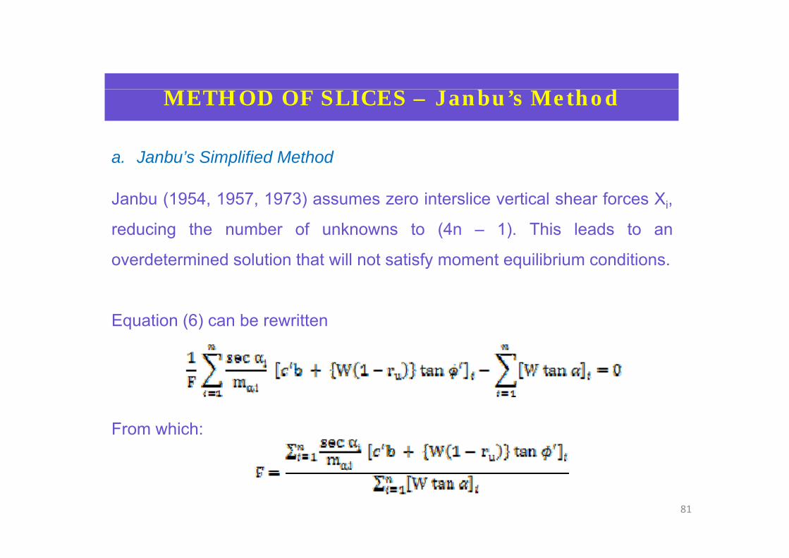
a. Janbu’s Simplified Method

Janbu (1954, 1957, 1973) assumes zero interslice vertical shear forces Xi,

reducing the number of unknowns to (4n – 1). This leads to an

overdetermined solution that will not satisfy moment equilibrium conditions.

Equation (6) can be rewritten

From which:

81

b ’ h dMETHOD OF SLICES – Janbu’s Method

Th ti f ti l i t li f i l d FOSThe assumption of zero vertical interslice forces give an overvalued FOS.

To account for this inadequacy, Janbu presented a correction factor, f0 (>1),

so that:so that:

This modification factor is a function of the slide geometry and the strengthg y g

parameters of the soil.There is no consensus concerning the

selection of the appropriate f0 value for

a surface intersecting different soil

types. In cases where such a mixed

variety of soils is present, the c – φ

curve is generally used to correct the

calculated FOS value. 82

b ’ h dMETHOD OF SLICES – Janbu’s Method

F i thi difi ti f t l b l l t d diFor convenience, this modification factor can also be calculated according

to the formula

where b1 varies according to the soil type:1 g yp

c only soils: b1 = 0.69

φ only soils: b1 = 0.31φ y 1

c and φ soils: b1 = 0.5

83

d d h dMETHOD OF SLICES – Advanced Methods

M t P i M th d M t d P i (1965)Morgenstern – Price Method Morgenstern and Price (1965) propose a

method in which the inclination of the interslice resultant force is assumed

to vary according to a “portion” of an arbitrary function i eto vary according to a portion of an arbitrary function, i.e.

Xi / Ei = λ f(x)

This additional “portion” of a selected function introduces an additionalThis additional portion of a selected function introduces an additional

unknown, leaving 4n unknowns and 4n equations.

The Morgenstern – Price Method satisfy equations (6) and (8) and then theThe Morgenstern Price Method satisfy equations (6) and (8) and then the

force and moment equilibrium for any kind of failure surface.

Spencer’s Method Spencer (1967, 1973) rigorously satisfies static

equilibrium by assuming that the resultant interslice force has a constant,

but unknown, inclination. This method derives from Morgenstern – Price

Method, assuming f(x) = cost. 84

A l li it ilib i (GLE) f l ti (Ch h 1986 F dl d t l

METHOD OF SLICES – GLE

A general limit equilibrium (GLE) formulation (Chugh, 1986; Fredlund et al.,

1981) can be developed to encompass most of the assumptions used by

the various methods and may be used to analyze circular and noncircularthe various methods and may be used to analyze circular and noncircular

failure surfaces.

In view of this universal applicability, the GLE formulation has become one

of the most popular methods as its generalization offers the ability to model

a discrete version of the Morgenstern and Price (1965) procedure via the

function used to describe the distribution of the interslice force angles.

The method can be used to satisfy either force and moment equilibrium or,

if required, just the force equilibrium conditions.if required, just the force equilibrium conditions.

85

Th GLE d li th l ti f i t f ti th t

METHOD OF SLICES – GLE

The GLE procedure relies on the selection of an appropriate function that

describes the variation of the interslice force angles to satisfy complete

equilibriumequilibrium.

The main difficulty in using the GLE procedure is related to the requirementThe main difficulty in using the GLE procedure is related to the requirement

that the user verify the reliability and “reasonableness” of the calculated

FOS This additional complexity prevents the general use of the GLEFOS. This additional complexity prevents the general use of the GLE

method for automatic search procedures that attempt to identify the critical

failure surface. However, single failure surfaces can be analyzed and thefailure surface. However, single failure surfaces can be analyzed and the

detailed solution examined for reasonableness.

86

Sl t bilit h t f l f li i l i t

STABILITY CHARTS

Slope stability charts are useful for preliminary analysis, to compare

alternates that can later be examined by more detailed analyses.

Chart solutions also provide a rapid means of checking the results ofChart solutions also provide a rapid means of checking the results of

detailed analyses.

Another use for slope stability charts is to back calculate strength valuesAnother use for slope stability charts is to back-calculate strength values

for failed slopes to aid in planning remedial measures. This can be done by

assuming an FOS of unity for the conditions at failure and solving for theassuming an FOS of unity for the conditions at failure and solving for the

unknown shear strength.

The major shortcoming in using design charts is that most of them are for

ideal, homogeneous soil conditions, which are not encountered in practice., g , p

87

hi i l b k dSTABILITY CHARTS – historical background

88

l ’ h

T l (1948) d l d l t bilit h t f il ith φ 0 d φ 0

STABILITY CHARTS – Taylor’s Charts

Taylor (1948) developed slope stability charts for soils with φ = 0 and φ > 0.

As shown in these charts, the slope has an angle β, a height H, and base

stratum at a depth of D H below the toe where D is a depth ratiostratum at a depth of D·H below the toe, where D is a depth ratio.

The charts can be used to determine the developed cohesion, cd, as

shown by the solid curves, and n·H, which is the distance from the toe to

the failure circle, as indicated by the short dashed curve.

If there are loadings outside the toe that prevent the circle from passing

below the toe, the long dashed curve should be used to determine the

d l d h i N t th t th lid d th l d h ddeveloped cohesion. Note that the solid and the long dashed curves

converge as n approaches zero. The circle represented by the curves on

the left of n 0 do not pass belo the toe so the loading o tside the toethe left of n = 0 do not pass below the toe, so the loading outside the toe

has no influence on the developed cohesion. 89

l ’ hSTABILITY CHARTS – Taylor’s Charts

90

i h ’ h

Bi h d M t ’ P d (1960) i it l th

STABILITY CHARTS – Bishop-Morgenstern’s Charts

Bishop and Morgenstern’s Procedure (1960) is quite more complex than

Taylor’s Charts. Compared to Taylor’s method, this one, furthermore, can

take into account water pore pressure inside the sliding mass and on thetake into account water pore pressure inside the sliding mass and on the

failure surface through water pore pressure ratio ru:

Bishop and Morgenstern’s Procedure is suitable for effective stress

analysis in homogeneous soils.

The charts are based on two parameters that are called stability factors mThe charts are based on two parameters that are called stability factors m

and n, so the FOS is defined as

FOS = m – n ruFOS m n ru

91

i h ’ h

d d d l t


m and n depend on several parameters:

• β, slope angle;

• φ’ soil friction angle;• φ , soil friction angle;

• df = H1/H, depth factor

• c’ / (γ H) similar to Taylor’s stability number• c / (γ H), similar to Taylor s stability number

df has a small influence on the solution, so one can refer essentially to

three value of it: 1.00, 1.25, 1.50.

In the charts are treated three conditions: c’ / (γ H) = 0.05

c’ / (γ H) = 0.025

c’ / (γ H) = 0

In general, user’s condition is located between two of the previous

situations. 92

i h ’ h

N ll th f t ( l f il f ) i b


Normally, the user refers to an average ru (along failure surface) given by:

where hi is the piezometric height of each of the slices in which the sliding

mass can be subdivided.

Note: This method doesn’t give the critical surface, but gives information

about dfabout df.

Given a series of geometrical and geotechnical parameters, it does exist a

ru value indicated with ru,e, through FOS for df = 1.0 is equal to FOS for df =

1.25, so that:

93

i h ’ hSTABILITY CHARTS – Bishop-Morgenstern’s Charts

A l l it i t l f hi h i F F th t iAnalogously, it exists a value of ru which gives F1.25 = F1.5, that is

If the calculated average ru is greater than r’u,e, then F1.25 < F1, so the

diti ith d 1 25 i iti lcondition with df = 1.25 is more critical.

The same reasoning can be made comparing user’s situation with df = 1.25

condition and df = 1.5 condition for establish which is the most critical

situation.

94

i h ’ hSTABILITY CHARTS – Bishop-Morgenstern’s Charts

95

EG Slope Stability - Geoplanning · · 2012-02-13Geologic Conditions Potential Failure Surface...

Documents

Transcript of EG Slope Stability - Geoplanning · · 2012-02-13Geologic Conditions Potential Failure Surface...