EFFICIENTLY MODELING LONG SEQUENCES WITH …
28
Under review as a conference paper at ICLR 2022 E FFICIENTLY MODELING L ONG S EQUENCES WITH S TRUCTURED S TATE S PACES Anonymous authors Paper under double-blind review ABSTRACT A central goal of sequence modeling is designing a single principled model that can address sequence data across a range of modalities and tasks, particularly on long-range dependencies. Although conventional models including RNNs, CNNs, and Transformers have specialized variants for capturing long dependencies, they still struggle to scale to very long sequences of 10000 or more steps. A promising recent approach proposed modeling sequences by simulating the fundamental state space model (SSM) x 0 (t)= Ax(t)+ Bu(t),y(t)= Cx(t)+ Du(t), and showed that for appropriate choices of the state matrix A, this system could handle long-range dependencies mathematically and empirically. However, this method has prohibitive computation and memory requirements, rendering it infeasible as a general sequence modeling solution. We propose the Structured State Space (S3) model based on a new parameterization for the SSM, and show that it can be computed much more efficiently than prior approaches while preserving their theoretical strengths. Our technique involves conditioning A with a low-rank correction, allowing it to be diagonalized stably and reducing the SSM to the well-studied computation of a Cauchy kernel. S3 achieves strong empirical results across a diverse range of established benchmarks, including (i) 91% accuracy on sequential CIFAR-10 with no data augmentation or auxiliary losses, on par with a larger 2-D ResNet, (ii) substantially closing the gap to Transformers on image and language modeling tasks, while performing generation 60× faster (iii) SoTA on every task from the Long Range Arena benchmark, including solving the challenging Path-X task of length 16k that all prior work fails on, while being as efficient as all competitors. 1 I NTRODUCTION A central problem in sequence modeling is efficiently handling data that contains long-range depen- dencies (LRDs). Real-world time-series data often requires reasoning over tens of thousands of time steps, while few sequence models address even thousands of time steps. For instance, results from the long-range arena (LRA) benchmark (Tay et al., 2021) highlight that sequence models today perform poorly on LRD tasks, including one (Path-X) where no model performs better than random guessing. Since LRDs are perhaps the foremost challenge for sequence models, all standard model families such as continuous-time models (CTMs), RNNs, CNNs, and Transformers include many specialized variants designed to address them. Modern examples include orthogonal and Lipschitz RNNs (Arjovsky et al., 2016; Erichson et al., 2021) to combat vanishing gradients, dilated convolutions to increase context size (Bai et al., 2018; Oord et al., 2016), and an increasingly vast family of efficient Transformers that reduce the quadratic dependence on sequence length (Katharopoulos et al., 2020; Choromanski et al., 2020). Despite being designed for LRDs, these solutions still perform poorly on challenging benchmarks such as LRA (Tay et al., 2021) or raw audio classification (Gu et al., 2021). An alternative approach to LRDs was recently introduced based on the state space model (SSM) (Fig. 1). SSMs are a foundational scientific model used in fields such as control theory, computational neuroscience, and many more, but have not been applicable to deep learning for concrete theoretical reasons. In particular, Gu et al. (2021) showed that deep SSMs actually struggle even on simple tasks, but can perform exceptionally well when equipped with special state matrices A recently derived to solve a problem of continuous-time memorization (Voelker et al., 2019; Gu et al., 2020a). Their 1
Transcript of EFFICIENTLY MODELING LONG SEQUENCES WITH …

Under review as a conference paper at ICLR 2022
EFFICIENTLY MODELING LONG SEQUENCESWITH STRUCTURED STATE SPACES
Anonymous authorsPaper under double-blind review
ABSTRACT
A central goal of sequence modeling is designing a single principled model thatcan address sequence data across a range of modalities and tasks, particularly onlong-range dependencies. Although conventional models including RNNs, CNNs,and Transformers have specialized variants for capturing long dependencies, theystill struggle to scale to very long sequences of 10000 or more steps. A promisingrecent approach proposed modeling sequences by simulating the fundamentalstate space model (SSM) x′(t) = Ax(t) + Bu(t), y(t) = Cx(t) + Du(t), andshowed that for appropriate choices of the state matrix A, this system could handlelong-range dependencies mathematically and empirically. However, this methodhas prohibitive computation and memory requirements, rendering it infeasible asa general sequence modeling solution. We propose the Structured State Space(S3) model based on a new parameterization for the SSM, and show that it canbe computed much more efficiently than prior approaches while preserving theirtheoretical strengths. Our technique involves conditioning A with a low-rankcorrection, allowing it to be diagonalized stably and reducing the SSM to thewell-studied computation of a Cauchy kernel. S3 achieves strong empirical resultsacross a diverse range of established benchmarks, including (i) 91% accuracyon sequential CIFAR-10 with no data augmentation or auxiliary losses, on parwith a larger 2-D ResNet, (ii) substantially closing the gap to Transformers onimage and language modeling tasks, while performing generation 60× faster (iii)SoTA on every task from the Long Range Arena benchmark, including solving thechallenging Path-X task of length 16k that all prior work fails on, while being asefficient as all competitors.
1 INTRODUCTION
A central problem in sequence modeling is efficiently handling data that contains long-range depen-dencies (LRDs). Real-world time-series data often requires reasoning over tens of thousands of timesteps, while few sequence models address even thousands of time steps. For instance, results from thelong-range arena (LRA) benchmark (Tay et al., 2021) highlight that sequence models today performpoorly on LRD tasks, including one (Path-X) where no model performs better than random guessing.
Since LRDs are perhaps the foremost challenge for sequence models, all standard model familiessuch as continuous-time models (CTMs), RNNs, CNNs, and Transformers include many specializedvariants designed to address them. Modern examples include orthogonal and Lipschitz RNNs(Arjovsky et al., 2016; Erichson et al., 2021) to combat vanishing gradients, dilated convolutions toincrease context size (Bai et al., 2018; Oord et al., 2016), and an increasingly vast family of efficientTransformers that reduce the quadratic dependence on sequence length (Katharopoulos et al., 2020;Choromanski et al., 2020). Despite being designed for LRDs, these solutions still perform poorly onchallenging benchmarks such as LRA (Tay et al., 2021) or raw audio classification (Gu et al., 2021).
An alternative approach to LRDs was recently introduced based on the state space model (SSM)(Fig. 1). SSMs are a foundational scientific model used in fields such as control theory, computationalneuroscience, and many more, but have not been applicable to deep learning for concrete theoreticalreasons. In particular, Gu et al. (2021) showed that deep SSMs actually struggle even on simple tasks,but can perform exceptionally well when equipped with special state matrices A recently derivedto solve a problem of continuous-time memorization (Voelker et al., 2019; Gu et al., 2020a). Their
1

Under review as a conference paper at ICLR 2022
= 𝐴𝑥 + 𝐵𝑢𝑦 = 𝐶𝑥 + 𝐷𝑢
𝑥 = 𝑥 + ,𝐵𝑢𝑦 = 𝐶𝑥 + -𝐷𝑢
𝑦 = -𝐾 ∗ 𝑢𝐴 =
1 0 01 2 01 3 3
State Space Computational RepresentationsLong-Range
Dependencies
𝑥𝑢 𝑦
𝐴
Figure 1: (Left) State Space Models (SSM) parameterized by matrices A,B,C,D map an input signal u(t) tooutput y(t) through a latent state x(t). (Center) Recent theory on continuous-time memorization derives specialA matrices that allow SSMs to capture LRDs mathematically and empirically. (Right) SSMs can be computedeither as a recurrence (left) or convolution (right). However, materializing these conceptual views requiresutilizing different representations of its parameters (red, blue, green) which are very expensive to compute. S3introduces a novel parameterization that efficiently swaps between these representations, allowing it to handle awide range of tasks, be efficient at both training and inference, and excel at long sequences.
Linear State Space Layer (LSSL) conceptually unifies the strengths of CTM, RNN and CNN models,and provides a proof of concept that deep SSMs can address LRDs in principle.
Unfortunately, the LSSL is infeasible to use in practice because of prohibitive computation andmemory requirements induced by the state representation. For state dimension N and sequencelength L, computing the latent state requires O(N2L) operations and O(NL) space – compared toa Ω(L + N) lower bound for both. Thus for reasonably sized models (e.g. N = 256 in Gu et al.(2021)), the LSSL uses orders of magnitude more memory than comparably-sized RNNs or CNNs.Although theoretically efficient algorithms for the LSSL were proposed, we show that these arenumerically unstable. In particular, the special A matrix is highly non-normal in the linear algebraicsense, which prevents the application of conventional algorithmic techniques. Consequently, althoughthe LSSL showed that SSMs have strong performance, they are currently computationally impracticalas a general sequence modeling solution.
In this work, we introduce the Structured State Space (S3), an efficient deep sequence model basedon the SSM that solves the critical computational bottleneck in previous work. Technically, S3reparameterizes the structured state matrices A appearing in Voelker et al. (2019); Gu et al. (2020a)by decomposing them as the sum of a low-rank and skew-symmetric term. Additionally, instead ofexpanding the standard SSM in coefficient space, we compute its truncated generating function infrequency space, which can be simplified into a multipole-like evaluation. Combining these two ideas,we show that the low-rank term can be corrected by the Woodbury identity while the skew-symmetricterm can be diagonalized stably, ultimately reducing to a well-studied and theoretically stable Cauchykernel (Pan, 2001; 2017). This results in O(N + L) computation and O(N + L) memory usage,which is essentially tight for sequence models. Compared to the LSSL, S3 is up to 30× faster with400× less memory usage, while exceeding the LSSL’s performance empirically.
Empirically, S3 significantly advances the state-of-the-art for LRD. On the LRA benchmark forefficient sequence models, S3 is as fast as all baselines while outperforming them by 20+ pointson average. S3 is the first model to solve the difficult LRA Path-X task (length-16384), achieving93.7% accuracy compared to 50% random guessing for all prior work. On speech classificationwith length-16000 sequences, S3 almost halves the test error (2.4%) of specialized Speech CNNs –by contrast, all RNN and Transformer baselines fail to learn (≥ 70% error).
Towards a general-purpose sequence model. Beyond LRD, a broad goal of machine learning is todevelop a single model that can be used across a wide range of problems. Models today are typicallyspecialized to solve problems from a particular domain (e.g. images, audio, text, time-series), andenable a narrow range of capabilities (e.g. efficient training, fast generation, handling irregularlysampled data). This specialization is typically expressed via domain-specific preprocessing, inductivebiases, and architectures. Sequence models provide a general framework for solving many of theseproblems with reduced specialization – e.g. Vision Transformers for image classification with less
2

Under review as a conference paper at ICLR 2022
2D information (Dosovitskiy et al., 2020). However, most models such as Transformers generallystill require substantial specialization per task to achieve high performance.
Deep SSMs in particular have conceptual strengths that suggest they may be promising as a generalsequence modeling solution. These strengths include a principled approach to handling LRDs, as wellas the ability to move between continuous-time, convolutional, and recurrent model representations,each with distinct capabilities (Fig. 1). Our technical contributions enable SSMs to be appliedsuccessfully to a varied set of benchmarks with minimal modification:
• Large-scale generative modeling. On CIFAR-10 density estimation, S3 is competitive with the bestautoregressive models (2.85 bits per dim). On WikiText-103 language modeling, S3 substantiallycloses the gap to Transformers (within 0.8 perplexity), setting SoTA for attention-free models.
• Fast autoregressive generation. Like RNNs, S3 can use its latent state to perform 60× fasterpixel/token generation than standard autoregressive models on CIFAR-10 and WikiText-103.
• Irregularly sampled time-series. Like specialized CTMs, S3 can adapt to changes in time seriessampling frequency without retraining, e.g. at 0.5× frequency on speech classification.
• Learning with weaker inductive biases. With no architectural changes, S3 surpasses SpeechCNNs on speech classification, outperforms the specialized Informer model on 40/50 time-seriesforecasting problems, and matches a 2-D ResNet on sequential CIFAR with over 90% accuracy.
2 BACKGROUND: STATE SPACES
Sections 2.1 to 2.4 describe the four properties of SSMs in Fig. 1: the classic continuous-time repre-sentation, addressing LRDs with the HiPPO framework, the discrete-time recurrent representation,and the parallelizable convolution representation. In particular, Section 2.4 introduces the SSMconvolution kernel K, which is the focus of our theoretical contributions in Section 3.
2.1 STATE SPACE MODELS: A CONTINUOUS-TIME LATENT STATE MODEL
The state space model is defined by the simple equation (1). It maps a 1-D input signal u(t) to anN -D latent state x(t) before projecting to a 1-D output signal y(t).
x′(t) = Ax(t) + Bu(t)
y(t) = Cx(t) + Du(t)(1)
SSMs are broadly used in many scientific disciplines and related to latent state models such as HiddenMarkov Models (HMM). Our goal is to simply use the SSM as a black-box representation in a deepsequence model, where A,B,C,D are parameters learned by gradient descent. For the remainderof this paper, we will omit the parameter D for exposition (or equivalently, assume D = 0) becausethe term Du can be viewed as a skip connection and is easy to compute.
2.2 ADDRESSING LONG-RANGE DEPENDENCIES WITH HIPPO
Prior work found that the basic SSM (1) actually performs very poorly in practice. Intuitively, oneexplanation is that linear first-order ODEs solve to an exponential function, and thus may sufferfrom gradients scaling exponentially in the sequence length (i.e., the vanishing/exploding gradientsproblem (Pascanu et al., 2013)). To address this problem, the LSSL leveraged the HiPPO theoryof continuous-time memorization (Gu et al., 2020a). HiPPO specifies a class of certain matricesA ∈ RN×N that when incorporated into (1), allows the state x(t) to memorize the history of theinput u(t). The most important matrix in this class is defined by equation (2), which we will call theHiPPO matrix. For example, the LSSL found that simply modifying an SSM from a random matrixA to equation (2) improved its performance on the sequential MNIST benchmark from 50% to 98%.
(HiPPO Matrix) Ank =
(2n+ 1)1/2(2k + 1)1/2 if n > k
n+ 1 if n = k
0 if n < k
. (2)
3

Under review as a conference paper at ICLR 2022
2.3 DISCRETE-TIME SSM: THE RECURRENT REPRESENTATION
To be applied on a discrete input sequence (u0, u1, . . . ) instead of continuous function u(t), (1) mustbe discretized by a step size ∆ that represents the resolution of the input. Conceptually, the inputs ukcan be viewed as sampling an implicit underlying continuous signal u(t), where uk = u(k∆).
To discretize the continuous-time SSM, we follow prior work in using the bilinear method (Tustin,1947), which converts the state matrix A into an approximation A . The discrete SSM is
xk = Axk−1 + Buk A = (I −∆/2 ·A)−1(I + ∆/2 ·A)
yk = Cxk B = (I −∆/2 ·A)−1∆B C = C.(3)
Equation (3) is now a sequence-to-sequence map uk 7→ yk instead of function-to-function. Moreoverthe state equation is now a recurrence in xk, allowing the discrete SSM to be computed like an RNN.Concretely, xk ∈ RN can be viewed as a hidden state with transition matrix A.
Notationally, throughout this paper we use A,B, . . . to denote discretized SSM matrices definedby (3). Note that these matrices are a function of both A as well as a step size ∆; we suppress thisdependence for notational convenience when it is clear.
2.4 TRAINING SSMS: THE CONVOLUTIONAL REPRESENTATION
The recurrent SSM (3) is not practical for training on modern hardware due to its sequentiality.Instead, there is a well-known connection between linear time-invariant (LTI) SSMs such as (1) andcontinuous convolutions. Correspondingly, (3) can actually be written as a discrete convolution.
For simplicity let the initial state be x−1 = 0. Then unrolling (3) explicitly yields
x0 = Bu0 x1 = ABu0 + Bu1 x2 = A2Bu0 + ABu1 + Bu2 . . .
y0 = CBu0 y1 = CABu0 + CBu1 y2 = CA2Bu0 + CABu1 + CBu2 . . .
This can be vectorized into a convolution (4) with an explicit formula for the convolution kernel (5).
yk = CAkBu0 + CA
k−1Bu1 + · · ·+ CABuk−1 + Buk
y = K ∗ u.(4)
K ∈ RL := KL(A,B,C) :=(CA
iB)i∈[L]
= (CB,CAB, . . . ,CAL−1
B). (5)
In other words, equation (4) is a single (non-circular) convolution and can be computed very efficientlywith FFTs, provided that K is known. However, computing K in (5) is non-trivial and is the focusof our technical contributions in Section 3. We call K the SSM convolution kernel or filter.
3 METHOD: STRUCTURED STATE SPACES (S3)
Our technical results focus on developing the S3 parameterization and showing how to efficientlycompute all views of the SSM (Section 2): the continuous representation (A,B,C) (1), the recurrentrepresentation (A,B,C) (3), and the convolutional representation K (4).
Section 3.1 motivates our approach, which is based on the linear algebraic concepts of conjugation anddiagonalization, and discusses why the naive application of this approach does not work. Section 3.2gives an overview of the key technical components of our approach and formally defines the S3parameterization. Section 3.3 sketches the main results, showing that S3 is asymptotically efficient(up to log factors) for sequence models. Proofs are in Appendices B and C.
3.1 MOTIVATION: DIAGONALIZATION
The fundamental bottleneck in computing the discrete-time SSM (3) is that it involves repeated matrixmultiplication by A. For example, computing (5) naively as in the LSSL involves L successivemultiplications by A, requiring O(N2L) operations and O(NL) space.
To overcome this bottleneck, we use a structural result that allows us to simplify SSMs.
4

Under review as a conference paper at ICLR 2022
Algorithm 1 S3 CONVOLUTION KERNEL (SKETCH)
Input: S3 parameters Λ,p, q,B,C ∈ CN and step size ∆Output: SSM convolution kernel K = KL(A,B,C) for A = Λ− pq∗ (equation (5))
1: C ← C(I −A
L)
. Truncate SSM generating function (SSMGF) to length L
2:
[k00(ω) k01(ω)k10(ω) k11(ω)
]←[C p
]∗ ( 2∆
1−ω1+ω −Λ
)−1
[B p] . Black-box Cauchy kernel
3: K(ω)← 21+ω
[k00(ω)− k01(ω)(1 + k11(ω))−1k10(ω)
]. Woodbury Identity
4: K = K(ω) : ω = exp(2πi kL ) . Evaluate SSMGF at all roots of unity ω ∈ ΩL5: K ← iFFT(K) . Inverse Fourier Transform
Lemma 3.1. Conjugation is an equivalence relation on SSMs (A,B,C) ∼ (V −1AV ,V −1B,CV ).
Proof. Write out the two SSMs with state denoted by x and x respectively:
x′ = Ax+ Bu x′ = V −1AV x+ V −1Bu
y = Cx y = CV x
After multiplying the right side SSM by V , the two SSMs become identical with x = V x. Thereforethese compute the exact same operator u 7→ y, but with a change of basis by V in the state x.
Lemma 3.1 motivates putting A into a canonical form by conjugation1, which is ideally morestructured and allows faster computation. For example, if A were diagonal, the resulting computationsbecome much more tractable. In particular, the desired K (equation (4)) would be a Vandermondeproduct which theoretically only needs O((N +L) log2(N +L)) arithmetic operations (Pan, 2001).
Unfortunately, the naive application of diagonalization does not work due to numerical issues. First,Vandermonde multiplication is itself a famously ill-conditioned problem (Pan, 2016). Furthermore,we derive the explicit diagonalization for the HiPPO matrix (2) and show it has entries exponentiallylarge in the state sizeN , rendering the diagonalization numerically infeasible (e.g. CV in Lemma 3.1would not be computable). We note that Gu et al. (2021) proposed a different (unimplemented)algorithm to compute K faster than the naive algorithm. In Appendix B, we prove that it is alsonumerically unstable for related reasons.
Lemma 3.2. The HiPPO matrix A in equation (2) is diagonalized by the matrix Vij =(i+ji−j). In
particular, V3i,i =(
4i2i
)≈ 24i. Therefore V has entries of magnitude up to 24N/3.
3.2 THE S3 PARAMETERIZATION: NORMAL PLUS LOW-RANK
The previous discussion implies that we should only conjugate by well-conditioned matrices V . Theideal scenario is when the matrix A is diagonalizable by a perfectly conditioned (i.e., unitary) matrix.By the Spectral Theorem of linear algebra, this is exactly the class of normal matrices. However,this class of matrices is restrictive; in particular, it does not contain the HiPPO matrix (2).
We make the observation that although the HiPPO matrix is not normal, it can be decomposed as thesum of a normal and low-rank matrix. However, this is still not useful by itself: unlike a diagonalmatrix, powering up this sum (in (5)) is still slow and not easily optimized. We overcome thisbottleneck by simultaneously applying three new techniques.
• Instead of computing K directly, we compute its spectrum by evaluating its truncated generatingfunction
∑L−1j=0 Kjζ
j at the roots of unity ζ. K can then be found by applying an inverse FFT.
• This generating function is closely related to the matrix resolvent, and now involves a matrixinverse instead of power. The low-rank term can now be corrected by applying the Woodburyidentity which reduces (A + pq∗)−1 in terms of A−1, truly reducing to the diagonal case.
• Finally, we show that the diagonal matrix case is equivalent to the computation of a Cauchy kernel1
ωj−ζk , a well-studied problem with stable near-linear algorithms (Pan, 2015; 2017).
1Note that although we ultimately care about A, conjugation commutes with discretization.
5

Under review as a conference paper at ICLR 2022
Our techniques apply to any matrix that can be decomposed as Normal Plus Low-Rank (NPLR).Theorem 1. All HiPPO matrices from (Gu et al., 2020a) have a NPLR representation
A = V ΛV ∗ − pq> = V (Λ− V ∗p(V ∗q)∗)V ∗ (6)for unitary V ∈ CN×N , diagonal Λ, and low-rank factorization p, q ∈ RN×r. These matricesHiPPO- LegS, LegT, LagT all satisfy r = 1 or r = 2. In particular, equation (2) is NPLR with r = 1.
3.3 S3 ALGORITHMS AND COMPUTATIONAL COMPLEXITY
By equation (6), note that NPLR matrices can be conjugated into diagonal plus low-rank (DPLR)form (now overC instead ofR). Theorems 2 and 3 describe the complexities of SSMs where A is inDPLR form. S3 is optimal or near-optimal for both recurrent and convolutional representations.Theorem 2 (S3 Recurrence). Given any step size ∆, computing one step of the recurrence (3) canbe done in O(N) operations where N is the state size.
Theorem 2 follows from the fact that the inverse of a DPLR matrix is also DPLR (e.g. also by theWoodbury identity). This implies that the discretized matrix A is the product of two DPLR matricesand thus has O(N) matrix-vector multiplication. Appendix C.2 computes A in closed DPLR form.Theorem 3 (S3 Convolution). Given any step size ∆, computing the SSM convolution filter K canbe reduced to 4 Cauchy multiplies, requiring only O(N + L) operations and O(N + L) space.
Appendix C, Definition 3 formally defines Cauchy matrices, which are related to rational interpolationproblems. Computing with Cauchy matrices is an extremely well-studied problem in numericalanalysis, with both fast arithmetic and numerical algorithms based on the famous Fast MultipoleMethod (FMM) (Pan, 2001; 2015; 2017). The computational complexities of these algorithms undervarious settings are described in Appendix C, Proposition 5.
We reiterate that Theorem 3 is our core technical contribution, and its algorithm is the very motivationof the S3 parameterization. This algorithm is formally sketched in Algorithm 1.
3.4 ARCHITECTURE DETAILS OF THE DEEP S3 LAYER
Concretely, an S3 layer is parameterized as follows. First initialize a SSM with A set to the HiPPOmatrix (2). By Lemma 3.1 and Theorem 1, this SSM is unitarily equivalent to some (Λ−pq∗,B,C)for some diagonal Λ and vectors p, q,B,C ∈ CN×1. These comprise S3’s 5N trainable parameters.
The overall deep neural network (DNN) architecture of S3 is similar to prior work. As defined above,S3 defines a map from RL → RL, i.e. a 1-D sequence map. Typically, DNNs operate on featuremaps of sizeH instead of 1. S3 handles multiple features by simply definingH independent copies ofitself, and then mixing theH features with a position-wise linear layer for a total ofO(H2)+O(HN)parameters per layer. Overall, S3 defines a sequence-to-sequence map of shape (batch size, sequencelength, hidden dimension), exactly the same as related sequence models such as Transformers.
4 EXPERIMENTS
Section 4.1 benchmarks S3 against the LSSL and efficient Transformer models. Section 4.2 validatesS3 on LRDs: the LRA benchmark and raw speech classification. Section 4.3 investigates whether S3can be used as a general sequence model to perform effectively and efficiently in a wide variety ofsettings including image classification, image and text generation, and time series forecasting.
Table 1: Deep SSMs: The S3 parameterization with Algo-rithm 1 is asymptotically more efficient than the LSSL.
TRAINING STEP (MS) MEMORY ALLOC. (MB)
Dim. 128 256 512 128 256 512
LSSL 9.32 20.6 140.7 222.1 1685 13140S3 4.77 3.07 4.75 5.3 12.6 33.5
Ratio 1.9× 6.7× 29.6× 42.0× 133× 392×
Table 2: Benchmarks vs. efficient Transformers
LENGTH 1024 LENGTH 4096
Speed Mem. Speed Mem.
Transformer 1× 1× 1× 1×Performer 1.23× 0.43× 3.79× 0.086×Linear Trans. 1.58× 0.37× 5.35× 0.067×S3 1.58× 0.43× 5.19× 0.091×
6

Under review as a conference paper at ICLR 2022
Figure 2: Visualizations of a trained S3 model on LRA Path-X. SSM convolution kernels K ∈ R16384 arereshaped into a 128× 128 image. (Top) Filters from the first layer (Bottom) Filters from the last layer
4.1 S3 EFFICIENCY BENCHMARKS
We benchmark that S3 can be trained quickly and efficiently, both compared to the LSSL, as well asefficient Transformer variants designed for long-range sequence modeling. As outlined in Section 3,S3 is theoretically much more efficient than the LSSL, and Table 1 confirms that the S3 is orders ofmagnitude more speed- and memory-efficient for practical layer sizes. In fact, S3’s speed and memoryuse is competitive with the most efficient Transformer variants benchmarked by Tay et al. (2021)—Linear Transformer (Katharopoulos et al., 2020) and Performer (Choromanski et al., 2020)—in aparameter-matched setting (Table 2, following the protocol of Tay et al. (2021)).
4.2 LEARNING LONG RANGE DEPENDENCIES
As described in Sections 2.2 and 3.1, S3 uses a principled approach to address LRDs based onthe HiPPO theory of continuous-time memorization. Our goal in this section is to validate that S3achieves high performance on difficult tasks that require long-range reasoning. We focus here on twoproblems: (i) the Long-Range Arena, a well-known benchmark designed to test efficient sequencemodels on LRDs, and (ii) a speech classification problem as a real-world test of LRDs.
Long Range Arena (LRA). LRA (Tay et al., 2021) contains 6 tasks with lengths 1K-16K steps,encompassing modalities and objectives that require similarity, structural, and visuospatial reasoning.Table 3 compares S3 against the 11 Transformer variants from Tay et al. (2021) as well as follow-upwork. S3 substantially advances the SoTA, outperforming all baselines on all tasks and averaging80.88% compared to less than 60% for every baseline. Notably, S3 achieves over 93% on Path-X, anextremely challenging variant of the Pathfinder task that involves reasoning about LRDs with sparsesignal over sequences of length 16384. All previous models have failed (i.e. random guessing) due tomemory or computation bottlenecks, or simply being unable to learn such long dependencies.
We analyze S3’s performance on Path-X by visualizing its learned representations, in particular 1-Dconvolution kernels K which are the focus of our technical results in Section 3. Fig. 2 shows that S3learns a variety of filters that display spatially consistent structure and demonstrate awareness of the
Table 3: (Long Range Arena) Accuracy on full suite of LRA tasks. (Top) Original Transformer variants inLRA. Full results in Appendix D.2. (Bottom) Other models reported in the literature.
MODEL LISTOPS TEXT RETRIEVAL IMAGE PATHFINDER PATH-X AVG
Transformer 36.37 64.27 57.46 42.44 71.40 7 53.66Reformer 37.27 56.10 53.40 38.07 68.50 7 50.56BigBird 36.05 64.02 59.29 40.83 74.87 7 54.17Linear Trans. 16.13 65.90 53.09 42.34 75.30 7 50.46Performer 18.01 65.40 53.82 42.77 77.05 7 51.18
FNet 35.33 65.11 59.61 38.67 77.80 7 54.42Nystromformer 37.15 65.52 79.56 41.58 70.94 7 57.46Luna-256 37.25 64.57 79.29 47.38 77.72 7 59.37S3 58.35 73.15 87.09 86.97 86.05 93.68 80.88
7

Under review as a conference paper at ICLR 2022
Table 4: (Speech classification) Transformer, CTM,RNN, CNN, and SSM models. (MFCC) Standardpre-processed MFCC features (length-161). (Raw)Unprocessed signals (length-16000). (0 .5×) Fre-quency change at test time. 7 denotes not applicableor computationally infeasible on single GPU.
MFCC RAW 0.5×Transformer 90.75 7 7Performer 80.85 30.77 30.68
ODE-RNN 65.9 7 7NRDE 89.8 16.49 15.12
ExpRNN 82.13 11.6 10.8LipschitzRNN 88.38 7 7
CKConv 95.3 71.66 65.96WaveGAN-D 7 96.25 7
LSSL 93.58 7 7S3 93.96 97.57 90.29
Table 5: (Pixel-level 1-D image classification)Transformer, RNN, CNN, and SSM models. Ex-tended results + citations in Appendix D.
SMNIST PMNIST SCIFAR
Transformer 98.9 97.9 62.2
LSTM 98.9 95.11 63.01r-LSTM 98.4 95.2 72.2UR-LSTM 99.28 96.96 71.00UR-GRU 99.27 96.51 74.4HiPPO-RNN 98.9 98.3 61.1LMU-FFT - 98.49 -LipschitzRNN 99.4 96.3 64.2
TCN 99.0 97.2 -TrellisNet 99.20 98.13 73.42CKConv 99.32 98.54 63.74
LSSL 99.53 98.76 84.65S3 99.63 98.70 91.13
2-D nature of the data. In particular, the lower layers learn simple kernels that extract features fromjust a few rows of local context while ignoring the rest of the image. On the other hand, higher layersaggregate information globally across full columns of the image at varying spatial frequencies. Filtersin these higher layers span the entire context (16384 pixels), confirming S3’s ability to learn LRDs.
Raw Speech Classification. Speech is a typical real-world time series domain, involving signalssampled from an underlying physical process at high frequency. We perform speech classificationusing the Speech Commands dataset (Warden, 2018). While most sequence models for speechrely on extensive preprocessing (e.g. to MFCC features), we classify raw speech (length-16000)following Romero et al. (2021). S3 achieves 97.6% accuracy, higher than all baselines that usethe 100× shorter MFCC features, and validates that a powerful LRD model is able to extractmore information from the raw data and outperform hand-crafted pre-processing. Additionally, weinclude a baseline CNN specifically designed for raw speech, the discriminator from the WaveGANmodel (Donahue et al., 2019), which performs worse than S3 while having 90× more parameters andincorporating many more architectural heuristics (Appendix D.2).
4.3 S3 AS A GENERAL SEQUENCE MODEL
A key goal of sequence modeling research is to develop a single model that can be applied in manydomains (e.g. images, audio, text, time-series) with a broad range of capabilities (e.g. efficienttraining, fast generation, handling irregularly sampled data). As a fundamental scientific model,SSMs are a promising candidate that come with a range of capabilities, and S3’s strong results on LRDbenchmarks spanning images, text, and speech are evidence of S3’s potential as a general sequencemodel. In this section, we focus on understanding this question in more depth by highlighting keystrengths of S3 in settings that usually require specialized models. The tasks we focus on (generativemodeling, image classification, time-series forecasting) are considered as LRD tasks in the literature,and serve as additional validation that S3 handles LRDs efficiently.
Large-scale generative modeling. We investigate two well-studied image and text benchmarks tovalidate the scalability, flexibility, and efficiency of S3. These tasks require much larger models thanour previous tasks – up to 250M parameters.
First, CIFAR density estimation is a popular benchmark for autoregressive models, where images areflattened into a sequence of 3072 RGB subpixels that are predicted one by one. Table 6 shows thatwith no 2D inductive bias, S3 is competitive with the best models designed for this task.
Second, WikiText-103 is an established benchmark for language modeling, an important task forlarge-scale sequence models where tokens are predicted sequentially based on past context. AlthoughRNNs were the model of choice for many years, Transformers are now the dominant model insuch applications that contain data that is inherently discrete. We show that alternative modelsto Transformers can still be competitive in these settings. By simply taking a strong Transformer
8

Under review as a conference paper at ICLR 2022
Table 6: (CIFAR-10 density estimation) As a generic se-quence model, S3 is competitive with previous autoregressivemodels (measured in bits per dim.) while incorporating no 2Dinductive bias, and automatically has fast generation.
Model bpd 2D bias Images / sec
Transformer 3.47 None 0.32 (1×)Linear Transf. 3.40 None 17.85 (56×)PixelCNN 3.14 2D conv. -Row PixelRNN 3.00 2D BiLSTM -PixelCNN++ 2.92 2D conv. 19.19 (59.97×)Image Transf. 2.90 2D local attn. 0.54 (1.7×)PixelSNAIL 2.85 2D conv. + attn. 0.13 (0.4×)Sparse Transf. 2.80 2D sparse attn. -
S3 (base) 2.92 None 20.84 (65.1×)S3 (large) 2.85 None 3.36 (10.5×)
Table 7: (WikiText-103 language modeling) S3approaches the performance of Transformers withmuch faster generation. (Top) Transformer base-line which our implementation is based on, withattention replaced by S3. (Bottom) Attention-freemodels (RNNs and CNNs).
Model Params Test ppl. Tokens / sec
Transformer 247M 20.51 0.8K (1×)
GLU CNN 229M 37.2 -AWD-QRNN 151M 33.0 -LSTM + Hebb. - 29.2 -TrellisNet 180M 29.19 -Dynamic Conv. 255M 25.0 -TaLK Conv. 240M 23.3 -S3 250M 21.28 48K (60×)
baseline (Baevski & Auli, 2018) and replacing the self-attention layers, S3 substantially closes thegap to Transformers (within 0.8 ppl), setting SoTA for attention-free models by over 2 ppl.
Fast autoregressive inference. A prominent limitation of autoregressive models is inference speed(e.g. generation), since they require a pass over the full context for every new sample. Severalmethods have been specifically crafted to overcome this limitation such as the Linear Transformer, ahybrid Transformer/RNN that switches to a stateful, recurrent view at inference time for speed.
As a stateful model, SSMs automatically have this ability (Fig. 1). By switching to its recurrentrepresentation (Section 2.3), S3 requires constant memory and computation per time step – in contrastto standard autoregressive models which scale in the context length. On both CIFAR-10 and WikiText-103, we report the throughput of various models at generation time, with S3 around 60× faster than avanilla Transformer on both tasks (details in Appendix D.3.3).
Irregularly sampled data. As a continuous-time model, S3 automatically adapts to irregularly-sampled data, a challenging setting for time series with a dedicated line of work (Rubanova et al.,2019; De Brouwer et al., 2019; Kidger et al., 2020). Without re-training, S3 achieves 90% accuracy at0.5× the frequency on Speech Commands, simply by changing its internal step size ∆ (Section 2.3).
Learning with weaker inductive bias. Beyond our results on speech (Section 4.2), we furthervalidate that S3 can be applied with minimal modifications on two domains that typically require spe-cialized domain-specific preprocessing and architectures. First, we compare S3 to the Informer (Zhouet al., 2021), a new Transformer architecture that uses a complex encoder-decoder designed fortime-series forecasting problems. A simple application of S3 that treats forecasting as a genericsequence-to-sequence transformation (Appendix D.3.5) outperforms the Informer and other baselineson 40/50 settings across 5 forecasting tasks. Notably, S3 is better on the longest setting in each task,e.g. reducing MSE by 32% when forecasting 30 days of weather data (Appendix D.3.5).
Finally, we evaluate S3 on pixel-level sequential image classification tasks (Table 5), popular bench-marks which were originally LRD tests for RNNs (Arjovsky et al., 2016). Beyond LRDs, thesebenchmarks point to a recent effort of the ML community to solve vision problems with reduceddomain knowledge, in the spirit of models such as Vision Transformers (Dosovitskiy et al., 2020) andMLP-Mixer (Tolstikhin et al., 2021). Sequential CIFAR is a particularly challenging dataset whereoutside of SSMs, all sequence models have a gap of over 25% to a simple 2-D CNN. By contrast, S3is competitive with a larger ResNet18 (7.9M vs. 11.0M parameters), both with (93.16% vs. 95.62%)or without (91.12% vs. 89.46%) data augmentation. Moreover, it is much more robust to otherarchitectural choices (e.g. 90.46% vs. 79.52% when swapping BatchNorm for LayerNorm).
5 CONCLUSION
We introduce S3, a model that uses a new parameterization for the state space model’s continuous-time, recurrent, and convolutional views to efficiently model LRDs in a principled manner. Resultsacross a set of established benchmarks evaluating a diverse range of data modalities and modelcapabilities suggest that S3 has the potential to be an effective general sequence modeling solution.
9

Under review as a conference paper at ICLR 2022
REFERENCES
Martin Arjovsky, Amar Shah, and Yoshua Bengio. Unitary evolution recurrent neural networks. InThe International Conference on Machine Learning (ICML), pp. 1120–1128, 2016.
Alexei Baevski and Michael Auli. Adaptive input representations for neural language modeling.arXiv preprint arXiv:1809.10853, 2018.
Shaojie Bai, J Zico Kolter, and Vladlen Koltun. An empirical evaluation of generic convolutional andrecurrent networks for sequence modeling. arXiv preprint arXiv:1803.01271, 2018.
Shaojie Bai, J Zico Kolter, and Vladlen Koltun. Trellis networks for sequence modeling. In TheInternational Conference on Learning Representations (ICLR), 2019.
Shiyu Chang, Yang Zhang, Wei Han, Mo Yu, Xiaoxiao Guo, Wei Tan, Xiaodong Cui, MichaelWitbrock, Mark Hasegawa-Johnson, and Thomas S Huang. Dilated recurrent neural networks. InAdvances in Neural Information Processing Systems (NeurIPS), 2017.
Rewon Child, Scott Gray, Alec Radford, and Ilya Sutskever. Generating long sequences with sparsetransformers. arXiv preprint arXiv:1904.10509, 2019.
Narsimha Chilkuri and Chris Eliasmith. Parallelizing legendre memory unit training. The Interna-tional Conference on Machine Learning (ICML), 2021.
Krzysztof Choromanski, Valerii Likhosherstov, David Dohan, Xingyou Song, Andreea Gane, TamasSarlos, Peter Hawkins, Jared Davis, Afroz Mohiuddin, Lukasz Kaiser, et al. Rethinking attentionwith performers. In The International Conference on Learning Representations (ICLR), 2020.
Yann N Dauphin, Angela Fan, Michael Auli, and David Grangier. Language modeling with gatedconvolutional networks. In International conference on machine learning, pp. 933–941. PMLR,2017.
Edward De Brouwer, Jaak Simm, Adam Arany, and Yves Moreau. Gru-ode-bayes: Continuousmodeling of sporadically-observed time series. In Advances in Neural Information ProcessingSystems (NeurIPS), 2019.
Chris Donahue, Julian McAuley, and Miller Puckette. Adversarial audio synthesis. In ICLR, 2019.
Alexey Dosovitskiy, Lucas Beyer, Alexander Kolesnikov, Dirk Weissenborn, Xiaohua Zhai, ThomasUnterthiner, Mostafa Dehghani, Matthias Minderer, Georg Heigold, Sylvain Gelly, et al. Animage is worth 16x16 words: Transformers for image recognition at scale. arXiv preprintarXiv:2010.11929, 2020.
N Benjamin Erichson, Omri Azencot, Alejandro Queiruga, Liam Hodgkinson, and Michael WMahoney. Lipschitz recurrent neural networks. In International Conference on Learning Represen-tations, 2021.
Gene H Golub and Charles F Van Loan. Matrix computations, volume 3. JHU press, 2013.
Albert Gu, Tri Dao, Stefano Ermon, Atri Rudra, and Christopher Re. Hippo: Recurrent memory withoptimal polynomial projections. In Hugo Larochelle, Marc’Aurelio Ranzato, Raia Hadsell, Maria-Florina Balcan, and Hsuan-Tien Lin (eds.), Advances in Neural Information Processing Systems33: Annual Conference on Neural Information Processing Systems 2020, NeurIPS 2020, December6-12, 2020, virtual, 2020a. URL https://proceedings.neurips.cc/paper/2020/hash/102f0bb6efb3a6128a3c750dd16729be-Abstract.html.
Albert Gu, Caglar Gulcehre, Tom Le Paine, Matt Hoffman, and Razvan Pascanu. Improving thegating mechanism of recurrent neural networks. In The International Conference on MachineLearning (ICML), 2020b.
Albert Gu, Isys Johnson, Karan Goel, Khaled Saab, Tri Dao, Atri Rudra, and Christopher Re.Combining recurrent, convolutional, and continuous-time models with the structured learnablelinear state space layer. In Advances in Neural Information Processing Systems (NeurIPS), 2021.
10

Under review as a conference paper at ICLR 2022
Sepp Hochreiter and Jurgen Schmidhuber. Long short-term memory. Neural computation, 9(8):1735–1780, 1997.
Angelos Katharopoulos, Apoorv Vyas, Nikolaos Pappas, and Francois Fleuret. Transformers are rnns:Fast autoregressive transformers with linear attention. In International Conference on MachineLearning, pp. 5156–5165. PMLR, 2020.
Patrick Kidger, James Morrill, James Foster, and Terry Lyons. Neural controlled differential equationsfor irregular time series. arXiv preprint arXiv:2005.08926, 2020.
Mario Lezcano-Casado and David Martınez-Rubio. Cheap orthogonal constraints in neural networks:A simple parametrization of the orthogonal and unitary group. In The International Conference onMachine Learning (ICML), 2019.
Shuai Li, Wanqing Li, Chris Cook, Ce Zhu, and Yanbo Gao. Independently recurrent neural network(IndRNN): Building a longer and deeper RNN. In Proceedings of the IEEE Conference onComputer Vision and Pattern Recognition, pp. 5457–5466, 2018.
Vasileios Lioutas and Yuhong Guo. Time-aware large kernel convolutions. In International Confer-ence on Machine Learning, pp. 6172–6183. PMLR, 2020.
Stephen Merity, Nitish Shirish Keskar, James Bradbury, and Richard Socher. Scalable languagemodeling: Wikitext-103 on a single gpu in 12 hours. SysML, 2018.
Aaron van den Oord, Sander Dieleman, Heiga Zen, Karen Simonyan, Oriol Vinyals, Alex Graves,Nal Kalchbrenner, Andrew Senior, and Koray Kavukcuoglu. Wavenet: A generative model for rawaudio. arXiv preprint arXiv:1609.03499, 2016.
Victor Pan. Structured matrices and polynomials: unified superfast algorithms. Springer Science &Business Media, 2001.
Victor Pan. Fast approximate computations with cauchy matrices and polynomials. Mathematics ofComputation, 86(308):2799–2826, 2017.
Victor Y Pan. Transformations of matrix structures work again. Linear Algebra and Its Applications,465:107–138, 2015.
Victor Y Pan. How bad are vandermonde matrices? SIAM Journal on Matrix Analysis andApplications, 37(2):676–694, 2016.
Razvan Pascanu, Tomas Mikolov, and Yoshua Bengio. On the difficulty of training recurrent neuralnetworks. In International conference on machine learning, pp. 1310–1318, 2013.
Jack Rae, Chris Dyer, Peter Dayan, and Timothy Lillicrap. Fast parametric learning with activationmemorization. The International Conference on Machine Learning (ICML), 2018.
Prajit Ramachandran, Tom Le Paine, Pooya Khorrami, Mohammad Babaeizadeh, Shiyu Chang, YangZhang, Mark A Hasegawa-Johnson, Roy H Campbell, and Thomas S Huang. Fast generation forconvolutional autoregressive models. arXiv preprint arXiv:1704.06001, 2017.
David W Romero, Anna Kuzina, Erik J Bekkers, Jakub M Tomczak, and Mark Hoogendoorn. Ckconv:Continuous kernel convolution for sequential data. arXiv preprint arXiv:2102.02611, 2021.
Yulia Rubanova, Tian Qi Chen, and David K Duvenaud. Latent ordinary differential equationsfor irregularly-sampled time series. In Advances in Neural Information Processing Systems, pp.5321–5331, 2019.
T Konstantin Rusch and Siddhartha Mishra. Unicornn: A recurrent model for learning very long timedependencies. The International Conference on Machine Learning (ICML), 2021.
Tim Salimans, Andrej Karpathy, Xi Chen, and Diederik P Kingma. Pixelcnn++: Improving thepixelcnn with discretized logistic mixture likelihood and other modifications. arXiv preprintarXiv:1701.05517, 2017.
11

Under review as a conference paper at ICLR 2022
Yi Tay, Mostafa Dehghani, Samira Abnar, Yikang Shen, Dara Bahri, Philip Pham, Jinfeng Rao,Liu Yang, Sebastian Ruder, and Donald Metzler. Long range arena : A benchmark for efficienttransformers. In International Conference on Learning Representations, 2021. URL https://openreview.net/forum?id=qVyeW-grC2k.
Ilya Tolstikhin, Neil Houlsby, Alexander Kolesnikov, Lucas Beyer, Xiaohua Zhai, Thomas Un-terthiner, Jessica Yung, Daniel Keysers, Jakob Uszkoreit, Mario Lucic, et al. Mlp-mixer: Anall-mlp architecture for vision. arXiv preprint arXiv:2105.01601, 2021.
Trieu H Trinh, Andrew M Dai, Minh-Thang Luong, and Quoc V Le. Learning longer-term depen-dencies in RNNs with auxiliary losses. In The International Conference on Machine Learning(ICML), 2018.
Arnold Tustin. A method of analysing the behaviour of linear systems in terms of time series. Journalof the Institution of Electrical Engineers-Part IIA: Automatic Regulators and Servo Mechanisms,94(1):130–142, 1947.
Ashish Vaswani, Noam Shazeer, Niki Parmar, Jakob Uszkoreit, Llion Jones, Aidan N. Gomez,Lukasz Kaiser, and Illia Polosukhin. Attention is all you need. In Advances in Neural InformationProcessing Systems (NeurIPS), 2017.
Aaron Voelker, Ivana Kajic, and Chris Eliasmith. Legendre memory units: Continuous-time represen-tation in recurrent neural networks. In Advances in Neural Information Processing Systems, pp.15544–15553, 2019.
Aaron Russell Voelker. Dynamical systems in spiking neuromorphic hardware. PhD thesis, Universityof Waterloo, 2019.
Pete Warden. Speech commands: A dataset for limited-vocabulary speech recognition. ArXiv,abs/1804.03209, 2018.
Max A Woodbury. Inverting modified matrices. Memorandum report, 42:106, 1950.
Felix Wu, Angela Fan, Alexei Baevski, Yann N Dauphin, and Michael Auli. Pay less attention withlightweight and dynamic convolutions. In The International Conference on Learning Representa-tions (ICLR), 2019.
Haoyi Zhou, Shanghang Zhang, Jieqi Peng, Shuai Zhang, Jianxin Li, Hui Xiong, and Wancai Zhang.Informer: Beyond efficient transformer for long sequence time-series forecasting. In The Thirty-Fifth AAAI Conference on Artificial Intelligence, AAAI 2021, Virtual Conference, volume 35, pp.11106–11115. AAAI Press, 2021.
A DISCUSSION
Related Work. Our work is most closely related to a line of work originally motivated by aparticular biologically-inspired SSM, which led to mathematical models for addressing LRDs.Voelker (2019); Voelker et al. (2019) derived a non-trainable SSM motivated from approximatinga neuromorphic spiking model, and Chilkuri & Eliasmith (2021) showed that it could be sped upat train time with a convolutional view. Gu et al. (2020a) extended this special case to a generalcontinuous-time function approximation framework with several more special cases of A matricesdesigned for long-range dependencies. However, instead of using a true SSM, all of these works fixeda choice of A and built RNNs around it. Most recently, Gu et al. (2021) used the full (1) explicitly asa deep SSM model, exploring new conceptual views of SSMs, as well as allowing A to be trained.As mentioned in Section 1, their method used a naive instantiation of SSMs that suffered from anadditional factor of N in memory and N2 in computation.
Beyond this work, our technical contributions (Section 3) on the S3 parameterization and algorithmsare applicable to a broader family of SSMs including these investigated in prior works, and ourtechniques for working with these models may be of independent interest.
12

Under review as a conference paper at ICLR 2022
Implementation. The computational core of S3’s training algorithm is the Cauchy kernel discussedin Sections 3.2 and 3.3 and Appendix C.3. As described in Appendix C.3 Proposition 5, there aremany algorithms for it with differing computational complexities and sophistication. Our currentimplementation of S3 actually uses the naive O(NL) algorithm which is easily parallelized on GPUsand has more easily accessible libraries allowing it to be implemented; we leverage the pykeopslibrary for memory-efficient kernel operations. However, this library is a much more general librarythat may not be optimized for the Cauchy kernels used here, and we believe that a dedicated CUDAimplementation can be more efficient. Additionally, as discussed in this work, there are asymptoticallyfaster and numerically stable algorithms for the Cauchy kernel (Proposition 5). However, thesealgorithms are currently not implemented for GPUs due to a lack of previous applications that requirethem. We believe that more efficient implementations of these self-contained computational kernelsare possible, and that S3 (and SSMs at large) may have significant room for further improvements inefficiency.
B NUMERICAL INSTABILITY OF LSSL
This section proves the claims made in Section 3.1 about prior work. We first derive the explicitdiagonalization of the HiPPO matrix, confirming its instability because of exponentially large entries.We then discuss the proposed theoretically fast algorithm from (Gu et al., 2021) (Theorem 2) andshow that it also involves exponentially large terms and thus cannot be implemented.
B.1 HIPPO DIAGONALIZATION
Proof of Lemma 3.2. The HiPPO matrix (2) is equal, up to sign and conjugation by a diagonal matrix,to
A =
1−1 21 −3 3−1 3 −5 41 −3 5 −7 5−1 3 −5 7 −9 61 −3 5 −7 9 −11 7−1 3 −5 7 −9 11 −13 8
.... . .
Ank =
(−1)n−k(2k + 1) n > k
k + 1 n = k
0 n < k
.
Our goal is to show that this A is diagonalized by the matrix
V =
(i+ j
i− j
)ij
=
11 11 3 11 6 5 11 10 15 7 11 15 35 28 9 1...
. . .
,
or in other words that columns of this matrix are eigenvectors of A.
Concretely, we will show that the j-th column of this matrix v(j) with elements
v(j)i =
0 i < j(i+ji−j)
=(i+j2j
)i ≥ j
is an eigenvector with eigenvalue j + 1. In other words we must show that for all indices k ∈ [N ],
(Av(j))k =∑i
Akiv(j)i = (j + 1)v
(j)k . (7)
13

Under review as a conference paper at ICLR 2022
If k < j, then for all i inside the sum, either k < i or i < j. In the first case Aki = 0 and in thesecond case v
(j)i = 0, so both sides of equation (7) are equal to 0.
It remains to show the case k ≥ j, which proceeds by induction on k. Expanding equation (7) usingthe formula for A yields
(Av)(j)k =
∑i
Akiv(j)i =
k−1∑i=j
(−1)k−i(2i+ 1)
(i+ j
2j
)+ (k + 1)
(k + j
2j
).
In the base case k = j, the sum disappears and we are left with (Av(j))j = (j+1)(
2j2j
)= (j+1)v
(j)j ,
as desired.
Otherwise, the sum for (Av)(j)k is the same as the sum for (Av)
(j)k−1 but with sign reversed and a few
edge terms. The result follows from applying the inductive hypothesis and algebraic simplification:
(Av)(j)k = −(Av)
(j)k−1 − (2k − 1)
(k − 1 + j
2j
)+ k
(k − 1 + j
2j
)+ (k + 1)
(k + j
2j
)= −(j + 1)
(k − 1 + j
2j
)− (k − 1)
(k − 1 + j
2j
)+ (k + 1)
(k + j
2j
)= −(j + k)
(k − 1 + j
2j
)+ (k + 1)
(k + j
2j
)= −(j + k)
(k − 1 + j)!
(k − 1− j)!(2j)!+ (k + 1)
(k + j
2j
)= − (k + j)!
(k − 1− j)!(2j)!+ (k + 1)
(k + j
2j
)= −(k − j) (k + j)!
(k − j)!(2j)!+ (k + 1)
(k + j
2j
)= (j − k)(k + 1)
(k + j
2j
)+ (k + 1)
(k + j
2j
)= (j + 1)v
(j)k .
B.2 FAST BUT UNSTABLE LSSL ALGORITHM
Instead of diagonalization, Gu et al. (2021, Theorem 2) proposed a sophisticated fast algorithm tocompute
KL(A,B,C) = (CB,CAB, . . . ,CAL−1
B).
This algorithm runs in O(N log2N + L logL) operations and O(N + L) space. However, we nowshow that this algorithm is also numerically unstable.
There are several reasons for the instability of this algorithm, but most directly we can pinpoint aparticular intermediate quantity that they use.Definition 1. The fast LSSL algorithm computes coefficients of p(x), the characteristic polynomialof A, as an intermediate computation. Additionally, it computes the coefficients of its inverse, p(x)−1
(mod xL).
We now claim that this quantity is numerically unfeasible. We narrow down to the case when A = Iis the identity matrix. Note that this case is actually in some sense the most typical case: whendiscretizing the continuous-time SSM to discrete-time by a step-size ∆, the discretized transitionmatrix A is brought closer to the identity. For example, with the Euler discretization A = I + ∆A,we have A→ I as the step size ∆→ 0.
Lemma B.1. When A = I , the fast LSSL algorithm requires computing terms exponentially large inN .
14
Under review as a conference paper at ICLR 2022
Proof. The characteristic polynomial of I is
p(x) = det |I − xI| = (1− x)N .
These coefficients have size up to(NN2
)≈ 2N√
πN/2.
The inverse of p(x) has even larger coefficients. It can be calculated in closed form by the generalizedbinomial formula:
(1− x)−N =
∞∑k=0
(N + k − 1
k
)xk.
Taking this (mod xL), the largest coefficient is(N + L− 2
L− 1
)=
(N + L− 2
N − 1
)=
(L− 1)(L− 2) . . . (L−N + 1)
(N − 1)!.
When L = N − 1 this is (2(N − 1)
N − 1
)≈ 22N
√πN
already larger than the coefficients of (1− x)N , and only increases as L grows.
C S3 ALGORITHM DETAILS
This section proves the results of Section 3.3, providing complete details of our efficient algorithmsfor S3.
Appendices C.1 to C.3 prove Theorems 1 to 3 respectively.
C.1 NPLR REPRESENTATIONS OF HIPPO MATRICES
We first prove Theorem 1, showing that all HiPPO matrices for continuous-time memory fall underthe S3 normal plus low-rank (NPLR) representation.
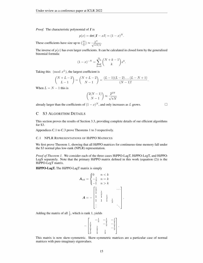
Proof of Theorem 1. We consider each of the three cases HiPPO-LagT, HiPPO-LegT, and HiPPO-LegS separately. Note that the primary HiPPO matrix defined in this work (equation (2)) is theHiPPO-LegT matrix.
HiPPO-LagT. The HiPPO-LagT matrix is simply
Ank =
0 n < k
− 12 n = k
−1 n > k
A = −
12 . . .1 1
21 1 1
21 1 1 1
2...
. . .
.
Adding the matrix of all 12 , which is rank 1, yields
−
− 1
2 − 12 − 1
212 − 1
2 − 12
12
12 − 1
212
12
12
.This matrix is now skew-symmetric. Skew-symmetric matrices are a particular case of normalmatrices with pure-imaginary eigenvalues.
15

Under review as a conference paper at ICLR 2022
Gu et al. (2020a) also consider a case of HiPPO corresponding to the generalized Laguerre polynomi-als that generalizes the above HiPPO-LagT case. In this case, the matrix A (up to conjugation by adiagonal matrix) ends up being close to the above matrix, but with a different element on the diagonal.After adding the rank-1 correction, it becomes the above skew-symmetric matrix plus a multiple ofthe identity. Thus after diagonalization by the same matrix as in the LagT case, it is still reduced todiagonal plus low-rank (DPLR) form, where the diagonal is now pure imaginary plus a real constant.
HiPPO-LegS. We restate the formula from equation (2) for convenience.
Ank = −
(2n+ 1)1/2(2k + 1)1/2 if n > k
n+ 1 if n = k
0 if n < k
.
Adding 12 (2n+ 1)1/2(2k + 1)1/2 to the whole matrix gives
−
12 (2n+ 1)1/2(2k + 1)1/2 if n > k12 if n = k
− 12 (2n+ 1)1/2(2k + 1)1/2 if n < k
Note that this matrix is not skew-symmetric, but is 12I + S where S is a skew-symmetric matrix.
This is diagonalizable by the same unitary matrix that diagonalizes S.
HiPPO-LegT.Up to the diagonal scaling, the LegT matrix is
A = −
1 −1 1 −1 . . .1 1 −1 11 1 1 −11 1 1 1...
. . .
.By adding −1 to this matrix and then the matrix2 2
2 2
the matrix becomes −2 −2
2−2
2 2
which is skew-symmetric. In fact, this matrix is the inverse of the Chebyshev Jacobi.
An alternative way to see this is as follows. The LegT matrix is the inverse of the matrix−1 1 0−1 1
−1 1−1 −1
This can obviously be converted to a skew-symmetric matrix by adding a rank 2 term. The inversesof these matrices are also rank-2 differences from each other by the Woodbury identity.
A final form is −1 1 −1 1−1 −1 1 −1−1 −1 −1 1−1 −1 −1 −1
+
1 0 1 00 1 0 11 0 1 00 1 0 1
=
0 1 0 1−1 0 1 00 −1 0 1−1 0 −1 0
This has the advantage that the rank-2 correction is symmetric (like the others), but the normalskew-symmetric matrix is now 2-quasiseparable instead of 1-quasiseparable.
16

Under review as a conference paper at ICLR 2022
C.2 COMPUTING THE S3 RECURRENT VIEW
We prove Theorem 2 showing the efficiency of the S3 parameterization for computing one step of therecurrent representation (Section 2.3).
Recall that without loss of generality, we can assume that the state matrix A = Λ− pq∗ is diagonalplus low-rank (DPLR), potentially over C. Our goal in this section is to explicitly write out a closedform for the discretized matrix A.
Recall from equation (3) thatA = (I −∆/2 ·A)−1(I + ∆/2 ·A)
B = (I −∆/2 ·A)−1∆B.
We first simplify both terms in the definition of A independently.
Forward discretization. The first term is essentially the Euler discretization motivated in Section 2.3.
I +∆
2A = I +
∆
2(Λ− pq∗)
=∆
2
[2
∆I + (Λ− pq∗)
]=
∆
2A0
where A0 is defined as the term in the final brackets.
Backward discretization. The second term is known as the Backward Euler’s method. Although thisinverse term is normally difficult to deal with, in the DPLR case we can simplify it using Woodbury’sIdentity (Proposition 4).(
I − ∆
2A
)−1
=
(I − ∆
2(Λ− pq∗)
)−1
=2
∆
[2
∆−Λ + pq∗
]−1
=2
∆
[D −Dp (1 + q∗Dp)
−1q∗D
]=
2
∆A1
where D =(
2∆ −Λ
)−1and A1 is defined as the term in the final brackets. Note that (1 + q∗Dp)
is actually a scalar, and A1 is actually itself a DPLR matrix.
S3 Recurrence. Finally, the full bilinear discretization can be rewritten in terms of these matrices asA = A1A0
B = A1∆B.
The discrete-time SSM (3) becomesxk = Axk−1 + Buk
= A1A0xk−1 + 2A1Bukyk = Cxk.
Note that A0,A1 are accessed only through matrix-vector multiplications. Since they are both DPLR,they have O(N) matrix-vector multiplication, showing Theorem 2.
C.3 COMPUTING THE CONVOLUTIONAL VIEW
The most involved part of using SSMs efficiently is computing K. This algorithm was sketched inSection 3.2 and is the main motivation for the S3 parameterization. In this section, we define thenecessary intermediate quantities and prove the main technical result.
The algorithm for Theorem 3 falls in roughly three stages. Assuming A has been conjugated intodiagonal plus low-rank form, we successively simplify the problem of computing K by applying thetechniques outlined in Section 3.2.
17

Under review as a conference paper at ICLR 2022
Reduction 0: Diagonalization By Lemma 3.1, we can switch the representation by conjugatingwith any unitary matrix. For the remainder of this section, we can assume that A is (complex)diagonal plus low-rank (DPLR).
Note that unlike diagonal matrices, a DPLR matrix does not lend itself to efficient computation ofK. The reason is that K computes terms CA
iB which involve powers of the matrix A. These are
trivially computable when A is diagonal, but is no longer possible for even simple modifications todiagonal matrices such as DPLR.
Reduction 1: SSM Generating Function To address the problem of computing powers of A,we introduce another technique. Instead of computing the SSM convolution filter K directly, weintroduce a generating function on its coefficients and compute evaluations of it.
Definition 2 (SSM Generating Function). We define the following quantities:
• The SSM convolution function is K(A,B,C) = (CB,CAB, . . . ) and the (truncated)SSM filter of length L
KL(A,B,C) = (CB,CAB, . . . ,CAL−1
B) ∈ RL (8)
• The SSM generating function at node z is
K(z;A,B,C) ∈ C :=
∞∑i=0
CAiBzi = C(I −Az)−1B (9)
and the truncated SSM generating function at node z is
KL(z;A,B,C) ∈ C :=
L−1∑i=0
CAiBzi = C(I −A
LzL)(I −Az)−1B (10)
• The truncated SSM generating function at nodes Ω ∈ CM is
KL(Ω;A,B,C) ∈ CM :=(KL(ωk;A,B,C)
)k∈[M ]
(11)
Intuitively, the generating function essentially converts the SSM convolution filter from the timedomain to frequency domain. Importantly, it preserves the same information, and the desired SSMconvolution filter can be recovered from evaluations of its generating function.
Lemma C.1. The SSM function KL(A,B,C) can be computed from the SSM generating functionKL(Ω;A,B,C at the roots of unity Ω = exp(2π kL : k ∈ [L] stably in O(L logL) operations.
Proof. For convenience define
K = KL(A,B,C)
K = KL(Ω;A,B,C).
Note that
Kj =
L−1∑k=0
Kk exp(2πijk
L).
Note that this is exactly the same as the Discrete Fourier Transform (DFT):
K = FLK.
Therefore K can be recovered from K with a single inverse DFT, which requires O(L logL)operations with the Fast Fourier Transform (FFT) algorithm.
18

Under review as a conference paper at ICLR 2022
Reduction 2: Woodbury Correction The primary motivation of Definition 2 is that it turns powersof A into a single inverse of A (equation (9)). While DPLR cannot be powered efficiently due to thelow-rank term, they can be inverted efficiently by the well-known Woodbury identity.Proposition 4 (Binomial Inverse Theorem or Woodbury matrix identity Woodbury (1950); Golub &Van Loan (2013)). Over a commutative ring R, let A ∈ RN×N and U ,V ∈ RN×p. Suppose Aand A + UV ∗ are invertible. Then Ip + V ∗A−1U ∈ Rp×p is invertible and
(A + UV ∗)−1 = A−1 −A−1U(Ip + V ∗A−1U)−1V ∗A−1
With this identity, we can convert the SSM generating function on a DPLR matrix A into one on justits diagonal component.Lemma C.2. Let A = Λ−pq∗ be a diagonal plus low-rank representation. Then for any evaluationnode z ∈ C, the truncated generating function satisfies
KL(z) =2
1 + z
[C∗R(z)−1B − C∗R(z)−1p
(1 + q∗R(z)−1p
)−1q∗R(z)−1B
]C = C(I −A
L)
R(z; Λ) =
(2
∆
1− z1 + z
−Λ
)−1
.
Proof. Directly expanding Definition 2 yields
KL(z;A,B,C) = C∗B + C
∗ABz + · · ·+ C
∗AL−1
BzL−1
= C∗ (
I −AL) (
I −Az)−1
B
= C∗(I −Az
)−1B
where C = C(I −A
L)
.
We can now explicitly expand the discretized SSM matrices A and B back in terms of the originalSSM parameters A and B. Lemma C.3 provides an explicit formula, which allows further simplifying
C∗(I −Az
)−1B =
2
1 + zC∗(
2
∆
1− z1 + z
−A
)−1
B
=2
1 + zC∗(
2
∆
1− z1 + z
− A + pq∗)−1
B
=2
1 + z
[C∗R(z)−1B − C∗R(z)−1p
(1 + q∗R(z)−1p
)−1q∗R(z)−1B
].
The last line applies the Woodbury Identity (Proposition 4) where R(z) =(
2∆
1−z1+z − A
)−1
.
The previous proof used the following self-contained result to back out the original SSM matricesfrom the discretization.Lemma C.3. Let A,B be the SSM matrices A,B discretized by the bilinear discretization with stepsize ∆. Then
C(I −A
)−1B =
2∆
1 + zC
[2
1− z1 + z
−∆A
]−1
B
Proof. Recall that the bilinear discretization that we use (equation (3)) is
A =
(I − ∆
2A
)−1(I +
∆
2A
)B =
(I − ∆
2A
)−1
∆B
19
Under review as a conference paper at ICLR 2022
The result is proved algebraic manipulations.
C(I −Az
)−1B = C
[(I − ∆
2A
)−1(I − ∆
2A
)−(I − ∆
2A
)−1(I +
∆
2A
)z
]−1
B
= C
[(I − ∆
2A
)−(I +
∆
2A
)z
]−1(I − ∆
2A
)B∆
= C
[I − z − ∆
2A(1 + z)
]−1
∆B
=∆
1− zC
[I − ∆A
2 1−z1+z
]−1
B
=2∆
1 + zC
[2
1− z1 + z
−∆A
]−1
B
Note that in the S3 parameterization, instead of constantly computing C = C(I −A
L)
, we can
simply reparameterize our parameters to learn C directly instead of C, saving a minor computationcost and simplifying the algorithm.
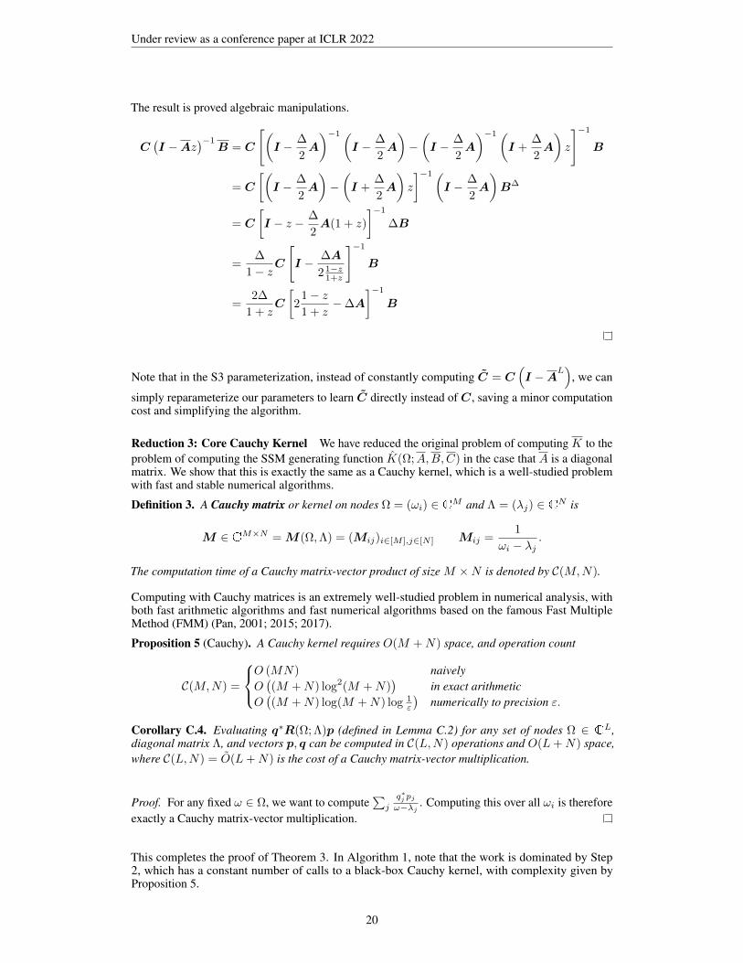
Reduction 3: Core Cauchy Kernel We have reduced the original problem of computing K to theproblem of computing the SSM generating function K(Ω;A,B,C) in the case that A is a diagonalmatrix. We show that this is exactly the same as a Cauchy kernel, which is a well-studied problemwith fast and stable numerical algorithms.
Definition 3. A Cauchy matrix or kernel on nodes Ω = (ωi) ∈ CM and Λ = (λj) ∈ CN is
M ∈ CM×N = M(Ω,Λ) = (Mij)i∈[M ],j∈[N ] Mij =1
ωi − λj.
The computation time of a Cauchy matrix-vector product of size M ×N is denoted by C(M,N).
Computing with Cauchy matrices is an extremely well-studied problem in numerical analysis, withboth fast arithmetic algorithms and fast numerical algorithms based on the famous Fast MultipleMethod (FMM) (Pan, 2001; 2015; 2017).
Proposition 5 (Cauchy). A Cauchy kernel requires O(M +N) space, and operation count
C(M,N) =
O (MN) naivelyO((M +N) log2(M +N)
)in exact arithmetic
O((M +N) log(M +N) log 1
ε
)numerically to precision ε.
Corollary C.4. Evaluating q∗R(Ω; Λ)p (defined in Lemma C.2) for any set of nodes Ω ∈ CL,diagonal matrix Λ, and vectors p, q can be computed in C(L,N) operations and O(L+N) space,where C(L,N) = O(L+N) is the cost of a Cauchy matrix-vector multiplication.
Proof. For any fixed ω ∈ Ω, we want to compute∑j
q∗j pjω−λj
. Computing this over all ωi is thereforeexactly a Cauchy matrix-vector multiplication.
This completes the proof of Theorem 3. In Algorithm 1, note that the work is dominated by Step2, which has a constant number of calls to a black-box Cauchy kernel, with complexity given byProposition 5.
20

Under review as a conference paper at ICLR 2022
Table 8: Full results for the Long Range Arena (LRA) benchmark for long-range dependencies in sequencemodels. (Top): Original Transformer variants in LRA. (Bottom): Other models reported in the literature.
Model LISTOPS TEXT RETRIEVAL IMAGE PATHFINDER PATH-X AVG
Random 10.00 50.00 50.00 10.00 50.00 50.00 36.67
Transformer 36.37 64.27 57.46 42.44 71.40 7 53.66Local Attention 15.82 52.98 53.39 41.46 66.63 7 46.71Sparse Trans. 17.07 63.58 59.59 44.24 71.71 7 51.03Longformer 35.63 62.85 56.89 42.22 69.71 7 52.88Linformer 35.70 53.94 52.27 38.56 76.34 7 51.14Reformer 37.27 56.10 53.40 38.07 68.50 7 50.56Sinkhorn Trans. 33.67 61.20 53.83 41.23 67.45 7 51.23Synthesizer 36.99 61.68 54.67 41.61 69.45 7 52.40BigBird 36.05 64.02 59.29 40.83 74.87 7 54.17Linear Trans. 16.13 65.90 53.09 42.34 75.30 7 50.46Performer 18.01 65.40 53.82 42.77 77.05 7 51.18
FNet 35.33 65.11 59.61 38.67 77.80 7 54.42Nystromformer 37.15 65.52 79.56 41.58 70.94 7 57.46Luna-256 37.25 64.57 79.29 47.38 77.72 7 59.37S3 58.35 73.15 87.09 86.97 86.05 93.68 80.88
D EXPERIMENT DETAILS AND FULL RESULTS
This section contains full experimental procedures and extended results and citations for our experi-mental evaluation in Section 4. Appendix D.1 corresponds to benchmarking results in Section 4.1,Appendix D.2 corresponds to LRD experiments (LRA and Speech Commands) in Section 4.2,and Appendix D.3 corresponds to the general sequence modeling experiments (generation, imageclassification, forecasting) in Section 4.3.
D.1 BENCHMARKING
Benchmarking results from Table 1 and Table 2 were tested on a single A100 GPU.
Benchmarks against LSSL For a given dimension H , a single LSSL or S3 layer was constructedwith H hidden features. For LSSL, the state size N was set to H as done in (Gu et al., 2021). For S3,the state size N was set to parameter-match the LSSL, which was a state size of N4 due to differencesin the parameterization. Table 1 benchmarks a single forward+backward pass of a single layer.
Benchmarks against Efficient Transformers Following (Tay et al., 2021), the Transformer mod-els had 4 layers, hidden dimension 256 with 4 heads, query/key/value projection dimension 128,and batch size 32, for a total of roughly 600k parameters. The S3 model was parameter tied whilekeeping the depth and hidden dimension constant (leading to a state size of N = 256).
We note that the relative orderings of these methods can vary depending on the exact hyperparametersettings. Other settings found S3 faster and more memory efficient than all Transformer variants, forexample when the query/key/value dimension was set to 256 instead of 128, as is more standard, andwhen the batch size is increased. However, we chose to report a setting closer to the ones in (Tayet al., 2021).
D.2 LONG-RANGE DEPENDENCIES
This section includes information for reproducing our experiments on the Long-Range Arena andSpeech Commands long-range dependency tasks.
Long Range Arena Table 8 contains extended results table with all 11 methods considered in (Tayet al., 2021).
For the S3 model, hyperparameters for all datasets are reported in Table 9. For all datasets, we usedthe AdamW optimizer with a constant learning rate schedule. The S3 state size was always fixed
21

Under review as a conference paper at ICLR 2022
Table 9: The values of the best hyperparameters found for classification datasets; LRA (Top) and images/speech(Bottom). LR is learning rate and WD is weight decay. BN and LN refer to Batch Normalization and LayerNormalization.
Depth Features H Norm Pre-norm Dropout LR Batch Size Epochs WD PatienceListOps 6 128 BN False 0 0.01 100 50 0.01 5Text 4 64 BN True 0 0.001 50 20 0 5Retrieval 6 256 BN True 0 0.002 64 20 0 20Image 6 1024 LN False 0.2 0.01 50 100 0.01 10Pathfinder 6 256 BN True 0.1 0.004 100 200 0 10Path-X 6 128 LN True 0.0 0.0002 16 100 0 20
CIFAR-10 6 1024 LN False 0.25 0.01 50 200 0.01 20
Speech Commands (MFCC) 4 256 LN False 0.2 0.01 100 50 0 5Speech Commands (Raw) 6 128 LN True 0.1 0.004 20 150 0 10
to N = 64. As S3 is a sequence-to-sequence model with output shape (batch, length, dimension)and LRA tasks are classification, mean pooling along the length dimension was applied after the lastlayer.
Hardware. All models were run on single GPU. Some tasks used an A100 GPU (notably, the Path-Xexperiments), which has a larger max memory of 40Gb. To reproduce these on smaller GPUs, thebatch size can be reduced or gradients can be accumulated for two batches.
Speech Commands We provide details of sweeps run for baseline methods run by us—numbersfor all others method are taken from Gu et al. (2021). The best hyperparameters used for S3 areincluded in Table 9.
Transformer (Vaswani et al., 2017) For MFCC, we swept the number of model layers 2, 4, dropout0, 0.1 and learning rates 0.001, 0.0005. We used 8 attention heads, model dimension 128,prenorm, positional encodings, and trained for 150 epochs with a batch size of 100. For Raw, theTransformer model’s memory usage made training impossible.
Performer (Choromanski et al., 2020) For MFCC, we swept the number of model layers 2, 4,dropout 0, 0.1 and learning rates 0.001, 0.0005. We used 8 attention heads, model dimension128, prenorm, positional encodings, and trained for 150 epochs with a batch size of 100. For Raw, weused a model dimension of 128, 4 attention heads, prenorm, and a batch size of 16. We reduced thenumber of model layers to 4, so the model would fit on the single GPU. We trained for 100 epochswith a learning rate of 0.001 and no dropout.
ExpRNN (Lezcano-Casado & Martınez-Rubio, 2019) For MFCC, we swept hidden sizes 256, 512and learning rates 0.001, 0.002, 0.0005. Training was run for 200 epochs, with a single layermodel using a batch size of 100. For Raw, we swept hidden sizes 32, 64 and learning rates0.001, 0.0005 (however, ExpRNN failed to learn).
Lipschitz RNN (Erichson et al., 2021) For MFCC, we swept hidden sizes 256, 512 and learningrates 0.001, 0.002, 0.0005. Training was run for 150 epochs, with a single layer model using abatch size of 100. For Raw, we found that LipschitzRNN was too slow to train on a single GPU(requiring a full day for 1 epoch of training alone).
WaveGAN Discriminator (Donahue et al., 2019) The WaveGAN-D in Table 4 is actually our improvedversion of the discriminator network from the recent WaveGAN model for speech (Donahue et al.,2019). This CNN actually did not work well out-of-the-box, and we added several features to help itperform better. The final model is highly specialized compared to our model, and includes:
• Downsampling or pooling between layers, induced by strided convolutions, that decreasethe sequence length between layers.
• A global fully-connected output layer; thus the model only works for one input sequencelength and does not work on MFCC features or the frequency-shift setting in Table 4.
• It only works with Batch Normalization turned on, whereas S3 works equally well witheither Batch Normalization or Layer Normalization.
• Almost 90× as many parameters as the S3 model (26.3M vs. 0.3M)
22
Under review as a conference paper at ICLR 2022
D.3 GENERAL SEQUENCE MODELING
This subsection corresponds to the experiments in Section 4.3. Because of the number of experimentsin this section, we use subsubsection dividers for different tasks to make it easier to follow: CIFAR-10density estimation Appendix D.3.1, WikiText-103 language modeling Appendix D.3.2, autoregres-sive generation Appendix D.3.3, sequential image classification Appendix D.3.4, and time-seriesforecasting Appendix D.3.5.
D.3.1 CIFAR DENSITY ESTIMATION
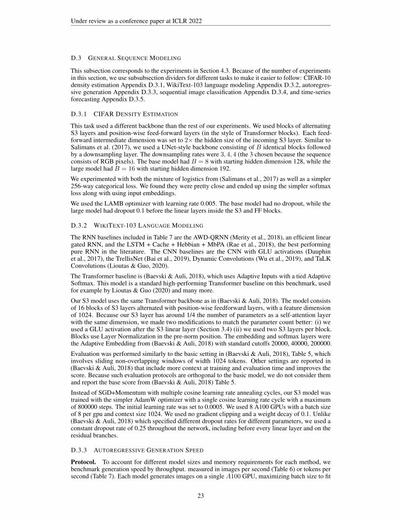
This task used a different backbone than the rest of our experiments. We used blocks of alternatingS3 layers and position-wise feed-forward layers (in the style of Transformer blocks). Each feed-forward intermediate dimension was set to 2× the hidden size of the incoming S3 layer. Similar toSalimans et al. (2017), we used a UNet-style backbone consisting of B identical blocks followedby a downsampling layer. The downsampling rates were 3, 4, 4 (the 3 chosen because the sequenceconsists of RGB pixels). The base model had B = 8 with starting hidden dimension 128, while thelarge model had B = 16 with starting hidden dimension 192.
We experimented with both the mixture of logistics from (Salimans et al., 2017) as well as a simpler256-way categorical loss. We found they were pretty close and ended up using the simpler softmaxloss along with using input embeddings.
We used the LAMB optimizer with learning rate 0.005. The base model had no dropout, while thelarge model had dropout 0.1 before the linear layers inside the S3 and FF blocks.
D.3.2 WIKITEXT-103 LANGUAGE MODELING
The RNN baselines included in Table 7 are the AWD-QRNN (Merity et al., 2018), an efficient lineargated RNN, and the LSTM + Cache + Hebbian + MbPA (Rae et al., 2018), the best performingpure RNN in the literature. The CNN baselines are the CNN with GLU activations (Dauphinet al., 2017), the TrellisNet (Bai et al., 2019), Dynamic Convolutions (Wu et al., 2019), and TaLKConvolutions (Lioutas & Guo, 2020).
The Transformer baseline is (Baevski & Auli, 2018), which uses Adaptive Inputs with a tied AdaptiveSoftmax. This model is a standard high-performing Transformer baseline on this benchmark, usedfor example by Lioutas & Guo (2020) and many more.
Our S3 model uses the same Transformer backbone as in (Baevski & Auli, 2018). The model consistsof 16 blocks of S3 layers alternated with position-wise feedforward layers, with a feature dimensionof 1024. Because our S3 layer has around 1/4 the number of parameters as a self-attention layerwith the same dimension, we made two modifications to match the parameter count better: (i) weused a GLU activation after the S3 linear layer (Section 3.4) (ii) we used two S3 layers per block.Blocks use Layer Normalization in the pre-norm position. The embedding and softmax layers werethe Adaptive Embedding from (Baevski & Auli, 2018) with standard cutoffs 20000, 40000, 200000.
Evaluation was performed similarly to the basic setting in (Baevski & Auli, 2018), Table 5, whichinvolves sliding non-overlapping windows of width 1024 tokens. Other settings are reported in(Baevski & Auli, 2018) that include more context at training and evaluation time and improves thescore. Because such evaluation protocols are orthogonal to the basic model, we do not consider themand report the base score from (Baevski & Auli, 2018) Table 5.
Instead of SGD+Momentum with multiple cosine learning rate annealing cycles, our S3 model wastrained with the simpler AdamW optimizer with a single cosine learning rate cycle with a maximumof 800000 steps. The initial learning rate was set to 0.0005. We used 8 A100 GPUs with a batch sizeof 8 per gpu and context size 1024. We used no gradient clipping and a weight decay of 0.1. Unlike(Baevski & Auli, 2018) which specified different dropout rates for different parameters, we used aconstant dropout rate of 0.25 throughout the network, including before every linear layer and on theresidual branches.
D.3.3 AUTOREGRESSIVE GENERATION SPEED
Protocol. To account for different model sizes and memory requirements for each method, webenchmark generation speed by throughput. measured in images per second (Table 6) or tokens persecond (Table 7). Each model generates images on a single A100 GPU, maximizing batch size to fit
23
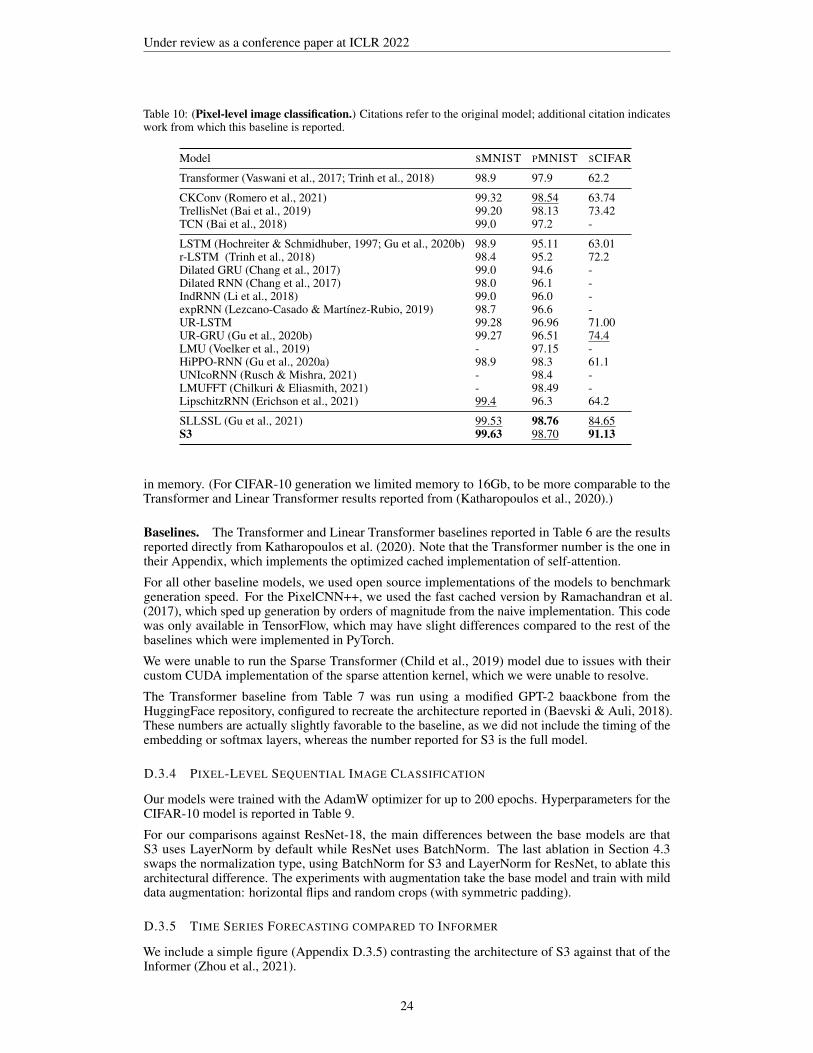
Under review as a conference paper at ICLR 2022
Table 10: (Pixel-level image classification.) Citations refer to the original model; additional citation indicateswork from which this baseline is reported.
Model SMNIST PMNIST SCIFAR
Transformer (Vaswani et al., 2017; Trinh et al., 2018) 98.9 97.9 62.2
CKConv (Romero et al., 2021) 99.32 98.54 63.74TrellisNet (Bai et al., 2019) 99.20 98.13 73.42TCN (Bai et al., 2018) 99.0 97.2 -
LSTM (Hochreiter & Schmidhuber, 1997; Gu et al., 2020b) 98.9 95.11 63.01r-LSTM (Trinh et al., 2018) 98.4 95.2 72.2Dilated GRU (Chang et al., 2017) 99.0 94.6 -Dilated RNN (Chang et al., 2017) 98.0 96.1 -IndRNN (Li et al., 2018) 99.0 96.0 -expRNN (Lezcano-Casado & Martınez-Rubio, 2019) 98.7 96.6 -UR-LSTM 99.28 96.96 71.00UR-GRU (Gu et al., 2020b) 99.27 96.51 74.4LMU (Voelker et al., 2019) - 97.15 -HiPPO-RNN (Gu et al., 2020a) 98.9 98.3 61.1UNIcoRNN (Rusch & Mishra, 2021) - 98.4 -LMUFFT (Chilkuri & Eliasmith, 2021) - 98.49 -LipschitzRNN (Erichson et al., 2021) 99.4 96.3 64.2
SLLSSL (Gu et al., 2021) 99.53 98.76 84.65S3 99.63 98.70 91.13
in memory. (For CIFAR-10 generation we limited memory to 16Gb, to be more comparable to theTransformer and Linear Transformer results reported from (Katharopoulos et al., 2020).)
Baselines. The Transformer and Linear Transformer baselines reported in Table 6 are the resultsreported directly from Katharopoulos et al. (2020). Note that the Transformer number is the one intheir Appendix, which implements the optimized cached implementation of self-attention.
For all other baseline models, we used open source implementations of the models to benchmarkgeneration speed. For the PixelCNN++, we used the fast cached version by Ramachandran et al.(2017), which sped up generation by orders of magnitude from the naive implementation. This codewas only available in TensorFlow, which may have slight differences compared to the rest of thebaselines which were implemented in PyTorch.
We were unable to run the Sparse Transformer (Child et al., 2019) model due to issues with theircustom CUDA implementation of the sparse attention kernel, which we were unable to resolve.
The Transformer baseline from Table 7 was run using a modified GPT-2 baackbone from theHuggingFace repository, configured to recreate the architecture reported in (Baevski & Auli, 2018).These numbers are actually slightly favorable to the baseline, as we did not include the timing of theembedding or softmax layers, whereas the number reported for S3 is the full model.
D.3.4 PIXEL-LEVEL SEQUENTIAL IMAGE CLASSIFICATION
Our models were trained with the AdamW optimizer for up to 200 epochs. Hyperparameters for theCIFAR-10 model is reported in Table 9.
For our comparisons against ResNet-18, the main differences between the base models are thatS3 uses LayerNorm by default while ResNet uses BatchNorm. The last ablation in Section 4.3swaps the normalization type, using BatchNorm for S3 and LayerNorm for ResNet, to ablate thisarchitectural difference. The experiments with augmentation take the base model and train with milddata augmentation: horizontal flips and random crops (with symmetric padding).
D.3.5 TIME SERIES FORECASTING COMPARED TO INFORMER
We include a simple figure (Appendix D.3.5) contrasting the architecture of S3 against that of theInformer (Zhou et al., 2021).
24

Under review as a conference paper at ICLR 2022
Forecast
S3 Layers
Context Forecast Window
encode
Decoder
Outputs
Masked Multi-head
ProbSparse
Self-attention
Multi-head
Attention
Encoder
Inputs: Xen
Concatenated Feature Map
Inputs: Xde=Xtoken, X0
0 0 0 0 0 0 0
Fully Connected Layer
Multi-head
ProbSparse
Self-attention
Multi-head
ProbSparse
Self-attention
Figure 3: Comparison of S3 and Informer (Zhou et al., 2021) models for forecasting tasks. (Left) S3 uses asimple sequence-to-sequence model; (Right) Informer uses a specialized encoder-decoder architecture designedspecifically for forecasting problems (figure taken from Zhou et al. (2021)).
Methods S3 Informer Informer† LogTrans Reformer LSTMa DeepAR ARIMA Prophet
Metric MSE MAE MSE MAE MSE MAE MSE MAE MSE MAE MSE MAE MSE MAE MSE MAE MSE MAE
ET
Th 1
24 0.061 0.191 0.098 0.247 0.092 0.246 0.103 0.259 0.222 0.389 0.114 0.272 0.107 0.280 0.108 0.284 0.115 0.27548 0.079 0.220 0.158 0.319 0.161 0.322 0.167 0.328 0.284 0.445 0.193 0.358 0.162 0.327 0.175 0.424 0.168 0.330168 0.104 0.258 0.183 0.346 0.187 0.355 0.207 0.375 1.522 1.191 0.236 0.392 0.239 0.422 0.396 0.504 1.224 0.763336 0.080 0.229 0.222 0.387 0.215 0.369 0.230 0.398 1.860 1.124 0.590 0.698 0.445 0.552 0.468 0.593 1.549 1.820720 0.116 0.271 0.269 0.435 0.257 0.421 0.273 0.463 2.112 1.436 0.683 0.768 0.658 0.707 0.659 0.766 2.735 3.253
ET
Th 2
24 0.095 0.234 0.093 0.240 0.099 0.241 0.102 0.255 0.263 0.437 0.155 0.307 0.098 0.263 3.554 0.445 0.199 0.38148 0.191 0.346 0.155 0.314 0.159 0.317 0.169 0.348 0.458 0.545 0.190 0.348 0.163 0.341 3.190 0.474 0.304 0.462168 0.167 0.333 0.232 0.389 0.235 0.390 0.246 0.422 1.029 0.879 0.385 0.514 0.255 0.414 2.800 0.595 2.145 1.068336 0.189 0.361 0.263 0.417 0.258 0.423 0.267 0.437 1.668 1.228 0.558 0.606 0.604 0.607 2.753 0.738 2.096 2.543720 0.187 0.358 0.277 0.431 0.285 0.442 0.303 0.493 2.030 1.721 0.640 0.681 0.429 0.580 2.878 1.044 3.355 4.664
ET
Tm
1
24 0.024 0.117 0.030 0.137 0.034 0.160 0.065 0.202 0.095 0.228 0.121 0.233 0.091 0.243 0.090 0.206 0.120 0.29048 0.051 0.174 0.069 0.203 0.066 0.194 0.078 0.220 0.249 0.390 0.305 0.411 0.219 0.362 0.179 0.306 0.133 0.30596 0.086 0.229 0.194 0.372 0.187 0.384 0.199 0.386 0.920 0.767 0.287 0.420 0.364 0.496 0.272 0.399 0.194 0.396288 0.160 0.327 0.401 0.554 0.409 0.548 0.411 0.572 1.108 1.245 0.524 0.584 0.948 0.795 0.462 0.558 0.452 0.574672 0.292 0.466 0.512 0.644 0.519 0.665 0.598 0.702 1.793 1.528 1.064 0.873 2.437 1.352 0.639 0.697 2.747 1.174
Wea
ther
24 0.125 0.254 0.117 0.251 0.119 0.256 0.136 0.279 0.231 0.401 0.131 0.254 0.128 0.274 0.219 0.355 0.302 0.43348 0.181 0.305 0.178 0.318 0.185 0.316 0.206 0.356 0.328 0.423 0.190 0.334 0.203 0.353 0.273 0.409 0.445 0.536168 0.198 0.333 0.266 0.398 0.269 0.404 0.309 0.439 0.654 0.634 0.341 0.448 0.293 0.451 0.503 0.599 2.441 1.142336 0.300 0.417 0.297 0.416 0.310 0.422 0.359 0.484 1.792 1.093 0.456 0.554 0.585 0.644 0.728 0.730 1.987 2.468720 0.245 0.375 0.359 0.466 0.361 0.471 0.388 0.499 2.087 1.534 0.866 0.809 0.499 0.596 1.062 0.943 3.859 1.144
EC
L
48 0.222 0.350 0.239 0.359 0.238 0.368 0.280 0.429 0.971 0.884 0.493 0.539 0.204 0.357 0.879 0.764 0.524 0.595168 0.331 0.421 0.447 0.503 0.442 0.514 0.454 0.529 1.671 1.587 0.723 0.655 0.315 0.436 1.032 0.833 2.725 1.273336 0.328 0.422 0.489 0.528 0.501 0.552 0.514 0.563 3.528 2.196 1.212 0.898 0.414 0.519 1.136 0.876 2.246 3.077720 0.428 0.494 0.540 0.571 0.543 0.578 0.558 0.609 4.891 4.047 1.511 0.966 0.563 0.595 1.251 0.933 4.243 1.415960 0.432 0.497 0.582 0.608 0.594 0.638 0.624 0.645 7.019 5.105 1.545 1.006 0.657 0.683 1.370 0.982 6.901 4.264
Count 22 5 0 0 0 0 2 0 0
Table 11: Univariate long sequence time-series forecasting results on four datasets (five cases).
In Appendix D.3.5, the goal is to forecast a contiguous range of future predictions (Green, length F) given a range of past context (Blue, length C ). We simply concatenate the entire context with asequence of masks set to the length of the forecast window. This input is a single sequence of lengthC + F that is run through the same simple deep S3 model used throughout this work, which maps toan output of length C + F . We then use just the last F features as the forecasted predictions.
Tables 11 and 12 contain full results on all 50 settings considered by Zhou et al. (2021). S3 sets thebest results on 40 out of 50 of these settings.
D.4 VISUALIZATIONS
We visualize the convolutional filter K learned by S3 for the Pathfinder and CIFAR-10 tasks inAppendix D.4 and Appendix D.4.
25

Under review as a conference paper at ICLR 2022
Figure 4: (Convolutional filters on Pathfinder) A random selection of filters learned by S3 in the first layer(top 4 rows) and last layer (bottom 4 rows) of the best model.
26

Under review as a conference paper at ICLR 2022
Figure 5: (Convolutional filters on sequential CIFAR) A random selection of filters learned by S3 in the firstlayer (top 4 rows) and last layer (bottom 4 rows) of the best model.
27

Under review as a conference paper at ICLR 2022
Methods S3 Informer Informer† LogTrans Reformer LSTMa LSTnet
Metric MSE MAE MSE MAE MSE MAE MSE MAE MSE MAE MSE MAE MSE MAE
ET
Th 1
24 0.525 0.542 0.577 0.549 0.620 0.577 0.686 0.604 0.991 0.754 0.650 0.624 1.293 0.90148 0.641 0.615 0.685 0.625 0.692 0.671 0.766 0.757 1.313 0.906 0.702 0.675 1.456 0.960168 0.980 0.779 0.931 0.752 0.947 0.797 1.002 0.846 1.824 1.138 1.212 0.867 1.997 1.214336 1.407 0.910 1.128 0.873 1.094 0.813 1.362 0.952 2.117 1.280 1.424 0.994 2.655 1.369720 1.162 0.842 1.215 0.896 1.241 0.917 1.397 1.291 2.415 1.520 1.960 1.322 2.143 1.380
ET
Th 2
24 0.871 0.736 0.720 0.665 0.753 0.727 0.828 0.750 1.531 1.613 1.143 0.813 2.742 1.45748 1.240 0.867 1.457 1.001 1.461 1.077 1.806 1.034 1.871 1.735 1.671 1.221 3.567 1.687168 2.580 1.255 3.489 1.515 3.485 1.612 4.070 1.681 4.660 1.846 4.117 1.674 3.242 2.513336 1.980 1.128 2.723 1.340 2.626 1.285 3.875 1.763 4.028 1.688 3.434 1.549 2.544 2.591720 2.650 1.340 3.467 1.473 3.548 1.495 3.913 1.552 5.381 2.015 3.963 1.788 4.625 3.709
ET
Tm
1
24 0.426 0.487 0.323 0.369 0.306 0.371 0.419 0.412 0.724 0.607 0.621 0.629 1.968 1.17048 0.580 0.565 0.494 0.503 0.465 0.470 0.507 0.583 1.098 0.777 1.392 0.939 1.999 1.21596 0.699 0.649 0.678 0.614 0.681 0.612 0.768 0.792 1.433 0.945 1.339 0.913 2.762 1.542288 0.824 0.674 1.056 0.786 1.162 0.879 1.462 1.320 1.820 1.094 1.740 1.124 1.257 2.076672 0.846 0.709 1.192 0.926 1.231 1.103 1.669 1.461 2.187 1.232 2.736 1.555 1.917 2.941
Wea
ther
24 0.334 0.385 0.335 0.381 0.349 0.397 0.435 0.477 0.655 0.583 0.546 0.570 0.615 0.54548 0.406 0.444 0.395 0.459 0.386 0.433 0.426 0.495 0.729 0.666 0.829 0.677 0.660 0.589168 0.525 0.527 0.608 0.567 0.613 0.582 0.727 0.671 1.318 0.855 1.038 0.835 0.748 0.647336 0.531 0.539 0.702 0.620 0.707 0.634 0.754 0.670 1.930 1.167 1.657 1.059 0.782 0.683720 0.578 0.578 0.831 0.731 0.834 0.741 0.885 0.773 2.726 1.575 1.536 1.109 0.851 0.757
EC
L
48 0.255 0.352 0.344 0.393 0.334 0.399 0.355 0.418 1.404 0.999 0.486 0.572 0.369 0.445168 0.283 0.373 0.368 0.424 0.353 0.420 0.368 0.432 1.515 1.069 0.574 0.602 0.394 0.476336 0.292 0.382 0.381 0.431 0.381 0.439 0.373 0.439 1.601 1.104 0.886 0.795 0.419 0.477720 0.289 0.377 0.406 0.443 0.391 0.438 0.409 0.454 2.009 1.170 1.676 1.095 0.556 0.565960 0.299 0.387 0.460 0.548 0.492 0.550 0.477 0.589 2.141 1.387 1.591 1.128 0.605 0.599
Count 18 5 6 0 0 0 0
Table 12: Multivariate long sequence time-series forecasting results on four datasets (five cases).
28