Efficient Wavelet-Based Scale Invariant Features … Wavelet-Based Scale Invariant Features Matching...

Efficient Wavelet-Based Scale Invariant Features Matching

SHWU-HUEY YEN1,a, NAN-CHIEH LIN1,b, HSIAO-WEI CHANG2,c Department of Computer Science and Information Engineering

Tamkang University1 151 Ying-Chuan Road, Tamsui, New Taipei City 25137, Taiwan

REPUBLIC OF CHINA Department of Computer Science and Information Engineering

China University of Science and Technology2

245, Sec. 3, Academia Road, Taipei 11581, Taiwan REPUBLIC OF CHINA

[email protected] [email protected]

[email protected]

Abstract: - Feature points’ matching is a popular method in dealing with object recognition and image matching problems. However, variations of images, such as shift, rotation, and scaling, influence the matching correctness. Therefore, a feature point matching system with a distinctive and invariant feature point detector as well as robust description mechanism becomes the main challenge of this issue. We use discrete wavelet transform (DWT) and accumulated map to detect feature points which are local maximum points on the accumulated map. DWT calculation is efficient compared to that of Harris corner detection or Difference of Gaussian (DoG) proposed by Lowe. Besides, feature points detected by DWT are located more evenly on texture area unlike those detected by Harris’ which are clustered on corners. To be scale invariant, the dominate scale (DS) is determined for each feature point. According to the DS of a feature point, an appropriate size of region centered at this feature point is transformed to log-polar coordinate system to improve the rotation and scale invariance. To enhance time efficiency and illumination robustness, we modify the contrast-based descriptors (CCH) proposed by Huang et al. Finally, in matching stage, a geometry constraint is used to improve the matching accuracy. Compared with existing methods, the proposed algorithm has better performance especially in scale invariance and blurring robustness. Key-Words: - Matching, Discrete Wavelet Transform (DWT), Dominate Scale (DS), Scale Invariance, Log-Polar Transform, Feature Point Descriptor 1 Introduction Many computer vision techniques, such as image retrieval and object recognition/tracking, have become more and more popular today. Robustness of feature points’ matching is a key to success of these applications. However, a small variation on images, such as shift, rotation and scaling, may affect the accuracy of feature point matching greatly. Therefore, to design a feature points matching system with robust detecting ability and invariant descriptor becomes the main challenge of this issue.

In 1977 Moravec developed an operator to locate “points of interest” which are also known as features, keypoints, or salient points in other research works. This operator is considered as a corner detector since it defines interest points as points where there is a large intensity variation in every direction. Moravec concluded that corners could be used to find matching regions in consecutive image frames [1][2]. The Moravec corner detector is

computationally efficient but it suffers from several problems. It is not rotation invariant, considered to have a noise response, and is susceptible to reporting false corners along edges and at isolated pixels. In 1988, Harris and Stephens developed an operator combing corner and edge detector by addressing the limitations of the Moravec operator [3]. The detector has desirable detection and repeatability rates which is why it has been widely used till now. However, the Harris corner detector still has some shortcomings. It is computationally demanding, sensitive to noise, has poor localization on many junction types, and it is not rotation invariant.

At first, corner detectors were designed for robotics and shape recognition and therefore, they may not be so suitable when applied to other applications [4]. In 1999, by taking Difference of Gaussian (DoG), Lowe presented a well-known scale-invariant feature transform (SIFT) algorithm.

WSEAS TRANSACTIONS on SIGNAL PROCESSING Shwu-Huey Yen, Nan-Chieh Lin, Hsiao-Wei Chang

ISSN: 1790-5052 121 Issue 4, Volume 7, October 2011

The SIFT features are invariant to image scale and rotation. They are also robust to changes in illumination, noise, and minor changes in viewpoint. To be highly distinctive, descriptors are computed in the image closed in scales to the keypoint’s scale. Histograms contain 8 bins (gradient orientations) each, and each descriptor contains a 4x4 array of histograms around the keypoint. This leads to a SIFT feature vector with 128 (=4x4x8) elements. For more information about SIFT, interested readers may refer to [5] [6]. There has been an extensive study done on the performance evaluation of different local descriptors, including SIFT, using a range of detectors [7]. The evaluation carried out suggests strongly that SIFT-based descriptors are the most robust and distinctive, and are therefore best suited for feature matching. Nevertheless, the complication of the SIFT algorithm made researchers continue to work on developing simpler algorithms in this topic.

The Discrete Wavelet Transform (DWT) provides a powerful framework to decompose images into different scales and orientations. In [4], they presented a wavelet-based salient point detector that extracts points on where variations occur in the image. To amend problems of shift variance and poor directional selectivity for diagonal features, Kingsbury suggested replacing DWT by Dual Tree Complex Wavelet Transform (DTCWT) [8]. Later on, they extended the DTCWT to a multi-scale keypoint detector [9]. An accumulated map is used to find robust keypoint scale selection. Compared to SIFT, their proposed method is shown to be more robust to rotation and less numerous. Also, DTCWT detector usually detects one keypoint per salient feature, which avoids producing too many redundant keypoints as in SIFT. However, besides keypoint detection by DTCWT, the descriptor design is also very important which is not discussed in [9].

Huang et al. [10] proposed a contrast-based descriptor called contrast context histogram (CCH). They proposed to extract the corners from a multi-scale Laplacian pyramid by Harris corner detector as feature points. CCH exploits the contrast properties of a local region centered at a feature point. Since it only evaluates the intensity differences between the center pixel (feature point) and the other pixels within the region, CCH is computationally efficient and invariant to rotation and linear illumination changes. However, the CCH is not scale invariant.

In this paper, we propose a wavelet-based feature point detector to combine with the CCH descriptor. The primary motivation is to develop an effective

feature point detecting system with a local descriptor that has smaller dimensionality. The computation simplicity and multi-scale properties are the reasons DWT is adopted. Accumulated map is used for feature points detecting. The local descriptors are computed in the image closed in scales, so called dominant scale (DS) determined by multi-scale of DWT, to the feature point’s scale. One novelty of the proposed algorithm is the size of region for calculating descriptor is accordance with the DS of the feature point. In this way, the feature points are not only computation efficient but also scale invariant. Since the accumulated map from DWT is used for feature points detecting, the problem of shift variance in DWT is not our concern. Also, since the orientation of the feature point is determined by its gradient, the poor directional selectivity of the DWT has no impact to our algorithm either.

The remaining of the paper is organized as follows. In Section 2, we describe the detail of our proposed method. Section 3 is the experimental results. The conclusion and future work are given in Section 4.

2 Proposed Method There are three main steps in our system: Feature Point Detection, Feature Point Descriptor and Feature Point Matching. Details are described in the following.

A. Feature Point Detection First we do the Discrete Wavelet Transformation (DWT) on the input image until the width or height of subband is not larger than 20 pixels. For example, an image with size 512×512 will do the DWT up to 5 levels. For each level i of the DWT, it generates three subbands Bib, b = 1, 2, 3 for HL, HH, LH. Equation (1) is to evaluate the energy magnitude Mi on level i.

βραρ )(3

1ib

b

ii ∏

=

= , (1)

where ρi is the coefficient of Mi, ρib is the magnitude of the coefficient on subband Bib, α and β are parameters. Setting low values for α and β will emphasis fine scales and improve the localization and detection of fine scale features, but it will make the detector sensitive to noise. In our experiments, α = 1 and β = 1/4 are used as recommended in [9] which claimed that this setting gives the best results



on different types of images. For each Mi, we use a bicubic interpolation

function to resize it to have the size of the input image, and use (2) to evaluate the accumulated map A.

∑=

=n

iif

1)M(A , (2)

where f is an interpolation function and n is the maximum level of DWT. The feature points are those local maximum of size 3×3 areas on A. Shown in Fig. 1, we compare the proposed feature points with the Harris corner feature points in Lena of 128×128. The image has 67 feature points detected by our method and 105 feature points by Harris corners. Unlike those shown in (b) which are close together, the feature points by DWT are located more evenly. Besides, feature points on the smooth texture connecting the ribbon to the hat are detected on (a) but not on (b). This shows that the proposed feature points are not only less in number but better represents the image comparing to Harris corners.

(a) (b)

Fig. 1 Feature points detected by (a) the proposed method and (b) Harris Corner Detector

After all the feature points are detected, DSp, the

Dominant Scale (DS) for a feature point p, is determined. DS is first proposed in [11] to have scale invariant property. If a feature point p is most prominent in a certain scale s, then p should have the strongest energy in the level i comparing to that on other levels assuming i is the level most close to such scale s. Thus, for a feature point p, the energies on all levels are compared and the level which has the largest energy is the DS of p as indicated in the Eq.(3).

{ } E ,...,E..., , Emax Arg DS 1p nii∀

= (3)

where Ei, the energy on level i, is the sum of corresponding position of feature point in three subbands of level i in DWT and n is the maximum level of DWT. The smaller value of DSp indicates that the feature point p has stronger reaction on lower level of DWT, and therefore a larger region around p should be included as sample data to calculate the feature point descriptor. On the other hand, the larger value of DSp represents that a smaller region around p should be included as sample data to calculate the descriptor. The diagram for feature point detection is shown at Fig. 2 where (1) & (2) means Eq.(1) & Eq.(2) are applied respectively.

Fig. 2 The diagram of feature point detection



B. Feature Point Descriptor We use DSp to decide the scale for R, a circular region for calculating local descriptor. As mentioned previously, larger DSp should choose smaller R and smaller DSp should choose larger R. Once R is decided, to be rotation invariant, a circular region of radius R/2 centered at the feature point p is used for calculating the descriptor. The circular area is then transformed to log-polar coordinate system that the circular area becomes a rectangular area. The transformation is accomplished by Eq.(4) and Eq.(5).

R

2sinr - 2R ,

R2cosr

2RI r) ,polar( ⎟⎟

⎠

⎞⎜⎜⎝

⎛⎟⎠⎞

⎜⎝⎛×⎟

⎠⎞

⎜⎝⎛×+=

πθπθθ

(4)

( ) log(r) ,polar ) ,(polar-log θδθ = , (5) where I(x, y) is the intensity of the sample within the circle, θ and r are the orientation axis and radius axis of the polar coordinate system. That is

2 20 0r ( ) ( )x x y y= − + −

and 1

0 0tan ( )y y x xθ −= − − , (6) where (x0, y0) is the feature point p. The advantage of the log-polar transformation (LPT) is two-fold. One is that objects occupying the center of Cartesian image become dominant over coarsely sampled background elements in the image periphery. And the other is that if image I2 is a rotation of image I1, then the difference of their LPTs is simply a translation in θ axis. As illustrated in Fig.3, (c) is a 90o rotation of (a), and (b), (d) are corresponding LPTs of (a) and (c). It is obvious that (d) is a translation of (b). The superimposed yellow curves depict the corresponding areas after transformation. Thus, in the matching problem, setting the orientation of the feature point as θ = 0 realizes the goal of rotation invariant.

After LPT, the obtained rectangular area, as in Fig. 3(b), is divided into 16 blocks with 2 equal parts in vertical (log(r)) and 8 equal parts in horizontal (θ). For each region k, a 2-bin histogram is constructed which records the average intensity differences that are above/below the intensity of the feature point [10]. Unlike CCH in [10] where the calculation is based on the intensity differences between the feature point and the other pixels in the region k, we calculate intensity differences between the mean intensity μ of a 3×3 window centered at

the feature point and the rest of pixels in the region k. By this way, the matching is more robust to possible small shifts of the feature points. Equations (7) and (8) define such histogram.

(a) (b)

(c) (d)

Fig. 3 Rotation effect on LPT (a) original image (c) original image rotated 90° (b) and (d) are the LPTs of (a) and (c) respectively

{ }

N xand Region x|-x

Hk

kRegion

k Region ++ ∑ >∈

=μμ

,

(7)

{ }

N xand Region x|-x

H -Region

k -Region

k

k

∑ <∈=

μμ,

(8)

where x is the intensity value of a pixel in the region k and μ is the mean intensity of a 3×3 window centered at the feature point, and N is number of points involved in the calculation. Finally, all these values of 16 regions are concatenated as a feature point descriptor of 32-dimension shown in (9).



( )-RegionRegion

-RegionRegion

-RegionRegion 16162211

H ,H ..., ,H ,H ,H ,H (p)Descriptor

+++

=

(9) C. Feature Point Matching For a query image Q and a target image T, the steps described above are applied such that all feature points are located and descriptors are evaluated. It is assumed that there are NQ and NT feature points in Q and T respectively. A matrix named Compare(Q,T) with size NQ×NT is constructed as in (10) to denote the distances of descriptors between feature points of Q and T where the distance d(p, p’) is defined in (11) with p, p’ are feature points of Q and T. The smaller it is meaning these two feature points are more likely to be the correct matching.

( ) ( ) ( )( ) ( ) ( )

( ) ( ) ( )⎥⎥⎥⎥⎥⎥

⎦

⎤

⎢⎢⎢⎢⎢⎢

⎣

⎡

=

TQQQ

T

T

NN2N1N

N22212

N12111

p' ,pd......p' ,pdp' ,pd..................

p' ,pdp' ,pdp' ,pdp' ,pd......p' ,pdp' ,pd

T)Compare(Q,

(10)

where

( ) )[k](p' Descriptor-(p)[k] Descriptor )p' d(p,32

1k

2∑=

=

(11)

In order to improve the matching accuracy, we use a simple geometric principle to ensure matching consistency. Three smallest values in Compare(Q,T) are located, say d(Pα , Pα ′), d(Pβ , Pβ ′), and d(Pγ , Pγ ′). If the figure formed by Pα , Pβ , Pγ in Q is similar to that formed by Pα ′, Pβ ′, Pγ ′ in T, then we call these points three basic points for Q and T respectively. Two figures are claimed to be similar if the corresponding ratios of three sides are similar enough. If these two figures are not similar, the next smallest value in Compare(Q,T) is picked to replace the biggest value of the three and check for similarity again. If all values in Compare(Q,T) have been checked and still can’t find the similar figures, these two images are claimed to be not matching.

Fig. 4 Three basic points in Q (left image) and T (right image) with feature point consistency relation

Suppose Pα , Pβ , Pγ and Pα′ , Pβ′ , Pγ′ are three

basic points found in Q and T, and we are looking for a matching for the feature point Pi of Q. For row i of the Compare(Q,T), if the smallest value is d(Pi, Pj), check for the consistency relation as illustrated in Fig. 4. That is to calculate the ratios Pi with basic points in Q corresponding to Pj with basic points in T. If Pi, P’

j are a matching pair then ratios defined in (12) should all equal to 1. However, in real applications with possible noises, Pi and P’

j are considered matched if ratios are close to 1 as defined in (13) where t is a given threshold. If t is small (e.g., 0.1) then matching accuracy will be improved but with possible high false negative, yet if t is large (e.g., 0.5) then the recall rate will be high with a price of increasing false positive. If the consistency relation in (13) is not satisfied for Pi, P’

j, and the next smallest value on row i is d(Pi, P’

l), then P’

l will replace P’j and the consistency relation

is checked again. If the consistency relation is failed for every point on row i, we claim Pi of Q has no matching in T.

pppp

r , pppp

r , p

pp r 321γ

γ

β

β

α

α

′′′ ′=

′=

′=

j

i

j

i

j

i

p. (12)

|r1/r2 - 1| < t and |r2/r3 - 1| < t and |r1/r3 - 1| < t.

(13) 3 The Experimental Results We compare the proposed method to the CCH method [10]. In CCH descriptors, feature vectors can be 32-dimension or 64-dimension. Our feature vectors are 32-dimension, therefore we choose 32-dimension feature descriptor of CCH for comparison. In order to compare the results, our algorithm and the CCH use the same feature matching method as described in C of the Section 2. The program is written by JCreator with JDK version 1.4, and the CPU is Intel Core 2 with 1.83 GHz clock rate. Memory size is 2GB. The testing



(a) (b) (c)

(d) (e) (f)

Fig. 5 The query images: (a) rotated 180° on Lina (i.e., R180(L)) (b) rotated 5° on Lina (i.e., R5(L)) (c) intensity changes on F-16 (i.e., I(F)) (d) Gaussian burring on Pepper (i.e., B(P)) (e) adding Gaussian noise on F-16 (i.e., N(F)) (f) JPEG compression on Pepper (i.e., J(P)) images are Lena(L), F-16(F), and Pepper(P) of 256×256. The query images are under several modifications- scaling, rotation, intensity change, adding Gaussian noise, Gaussian blurring, and JPEG compression- then find the matching features corresponding to the original images. The details of image modifications are the following: scaling (S)- the query image is halved (128×128), intensity (I)- the query image is 25% brighter than the original image, noise (N)- 3% of Gaussian noise is added to the query image, blurring (B)- Gaussian burring with a radius of 1.0 pixel is added, JPEG compression (J)- the query image is compressed then de-compressed with a compression quality of 4 (quality level is 1~12), rotation (R180 & R5)- the query image is rotated by 180 degrees and 5 degrees. All these image processes are done by Adobe Photoshop 6.0. Some of the query images are shown in Fig. 5.

In order to evaluate the effectiveness of the algorithm, two common criteria (14) and (15) are used.

points featurequery all ofnumber

points feature matchedcorrect ofnumber recall= ,

(14)

points feature matched ofnumber

points feature matchedcorrect ofnumber precision =

,

(15)

Recall and precision are real numbers between 0 and 1. The higher of the value in recall and precision indicates the better performance of the matching. However, the higher of the recall usually causes the lower of the precision, and the higher of the precision causes the lower of the recall. Therefore, F-measure that combines precision and recall by their harmonic mean is also adopted as given in (16). This is also known as the F1 measure, because recall and precision are evenly weighted. It is a special case of the general Fβ measure which was derived by van Rijsbergen. Fβ measures the effectiveness of retrieval with respect to a user who attaches β times as much importance to recall as precision [12].

precision recall2presision recall

F ⋅= ⋅

+. (16)



Table 1. Comparison on recall

Table 2. Comparison on precision

Partial experiment results are summarized in

Tables 1-3 for recall, precision, and F-measure. The t-value in Tables is the threshold t in (13) of the geometric constraint. When t is small (e.g., 0.1) then matching accuracy will be improved but with possible high false negative, yet if t is large (e.g., 0.5) then recall rate will be high with a price of increasing false positive. The labels under query in Tables are the modified query image (e.g., I(F) means a 25% intensity brightening has been applied on the image F-16; B(P) means a Gaussian blurring is applied on the image Pepper, etc.). In Tables, those bolded figures indicate the better performances and blue figures are the same performances between these two methods. The average on the right of the Table is considering performances for different threshold t-values on the same query image; and the average on the bottom of the Table is considering performances for different query images under the fixed t-value.

In changes of illumination (e.g., I(F)), both methods performed very well because the feature descriptors are based on the average in difference of intensities. It is worth noting that the intensity differences calculation in our method is based on the mean intensity of a 3×3 window centered at the feature point, while in CCH is based on only the feature point’s intensity. As the result indicates, the robustness has been improved by our method. When Gaussian noises are added to the query image (e.g., N(F)), more feature points are detected caused by noises. Thus precisions are not as good as recalls. The CCH method outperformed the proposed methods in recall, precision, and F-measure. In Gaussian blurring experiment (e.g., B(P)), the proposed method outperformed the CCH significantly. This indicates that corner features are vulnerable to blurring. The results also illustrates

RECALL Our method vs. CCH[10]

query t = 0.5 t = 0.4 t = 0.3 t = 0.2 t = 0.1 Ave

I(F) 0.98 0.94 0.98 0.92 0.96 0.91 0.93 0.87 0.90 0.83 0.950 0.894

N(F) 0.92 0.98 0.92 0.95 0.91 0.93 0.88 0.94 0.85 0.91 0.896 0.942

B(P) 0.96 0.59 0.96 0.59 0.97 0.56 0.97 0.50 0.97 0.42 0.966 0.532

J(P) 0.92 0.91 0.92 0.87 0.87 0.85 0.83 0.84 0.72 0.80 0.852 0.854

S(L) 0.88 0.71 0.87 0.66 0.82 0.60 0.75 0.57 0.63 0.45 0.790 0.598

R180(L) 0.86 0.85 0.80 0.81 0.77 0.76 0.69 0.68 0.58 0.58 0.740 0.736

R5(L) 0.84 0.83 0.81 0.79 0.78 0.75 0.66 0.65 0.55 0.54 0.728 0.712

Ave 0.909 0.830 0.894 0.799 0.869 0.766 0.816 0.721 0.743 0.647

PRECISION Our method vs. CCH[10]

query t = 0.5 t = 0.4 t = 0.3 t = 0.2 t = 0.1 Ave

I(F) 0.82 0.79 0.82 0.83 0.84 0.83 0.86 0.87 0.91 0.91 0.850 0.846

N(F) 0.83 0.86 0.83 0.87 0.84 0.88 0.86 0.89 0.89 0.92 0.850 0.884

B(P) 0.48 0.14 0.49 0.14 0.53 0.15 0.58 0.17 0.72 0.20 0.560 0.160

J(P) 0.96 0.68 0.95 0.73 0.91 0.74 0.88 0.75 0.82 0.79 0.904 0.738

S(L) 0.62 0.48 0.65 0.62 0.68 0.66 0.75 0.70 0.81 0.74 0.702 0.640

R180(L) 0.22 0.22 0.24 0.24 0.27 0.26 0.31 0.28 0.43 0.46 0.294 0.292

R5(L) 0.19 0.21 0.23 0.23 0.25 0.24 0.39 0.27 0.41 0.39 0.294 0.268

Ave 0.589 0.483 0.601 0.523 0.617 0.537 0.661 0.561 0.713 0.630



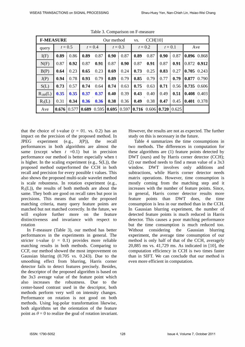
Table 3. Comparison on F-measure

that the choice of t-value (t = 01. vs. 0.2) has an impact on the precision of the proposed method. In JPEG experiment (e.g., J(P)), the recall performances in both algorithms are almost the same (except when t =0.1) but in precision performance our method is better especially when t is higher. In the scaling experiment (e.g., S(L)), the proposed method outperformed the CCH in both recall and precision for every possible t values. This also shows the proposed multi-scale wavelet method is scale robustness. In rotation experiment (e.g., R5(L)), the results of both methods are about the same. They both are good on recall rates but poor in precisions. This means that under the proposed matching criteria, many query feature points are matched but not matched correctly. In the future, we will explore further more on the feature distinctiveness and invariance with respect to rotation

In F-measure (Table 3), our method has better performances in the experiments in general. The stricter t-value (t = 0.1) provides more reliable matching results in both methods. Comparing to CCF, our method showed the most improvement on Gaussian blurring (0.705 vs. 0.243). Due to the smoothing effect from blurring, Harris corner detector fails to detect features precisely. Besides, the descriptor of the proposed algorithm is based on the 3x3 average value of the feature point which also increases the robustness. Due to the center-based contrast used in the descriptor, both methods perform very well on intensity changes. Performance on rotation is not good on both methods. Using log-polar transformation likewise, both algorithms set the orientation of the feature point as θ = 0 to realize the goal of rotation invariant.

However, the results are not as expected. The further study on this is necessary in the future.

Table 4 summarizes the time consumptions in two methods. The differences in computation for these algorithms are (1) feature points detected by DWT (ours) and by Harris corner detector (CCH); (2) our method needs to find a mean value of a 3x3 window. DWT involves only additions and subtractions, while Harris corner detector needs matrix operations. However, time consumption is mostly coming from the matching step and it increases with the number of feature points. Since, in general, Harris corner detector results more feature points than DWT does, the time consumption is less in our method than in the CCH. In Gaussian blurring experiment, the number of detected feature points is much reduced in Harris detector. This causes a poor matching performance but the time consumption is much reduced too. Without considering the Gaussian blurring experiment, the average time consumption of our method is only half of that of the CCH, averagely 20,885 ms vs. 41,729 ms. As indicated in [10], the computation efficiency in CCH is two times faster than in SIFT. We can conclude that our method is even more efficient in computation.

F-MEASURE Our method vs. CCH[10]

query t = 0.5 t = 0.4 t = 0.3 t = 0.2 t = 0.1 Ave

I(F) 0.89 0.86 0.89 0.87 0.90 0.87 0.89 0.87 0.90 0.87 0.896 0.868

N(F) 0.87 0.92 0.87 0.91 0.87 0.90 0.87 0.91 0.87 0.91 0.872 0.912

B(P) 0.64 0.23 0.65 0.23 0.69 0.24 0.73 0.25 0.83 0.27 0.705 0.243

J(P) 0.94 0.78 0.93 0.79 0.89 0.79 0.85 0.79 0.77 0.79 0.877 0.790

S(L) 0.73 0.57 0.74 0.64 0.74 0.63 0.75 0.63 0.71 0.56 0.735 0.606

R180(L) 0.35 0.35 0.37 0.37 0.40 0.39 0.43 0.40 0.49 0.51 0.408 0.403

R5(L) 0.31 0.34 0.36 0.36 0.38 0.36 0.49 0.38 0.47 0.45 0.401 0.378

Ave 0.676 0.577 0.689 0.595 0.695 0.597 0.716 0.606 0.720 0.625



Table 4. Comparison of time consumption (in ms)

Method Attack Proposed method CCH[10]

Scaling (S) 7288 20255

Rotated 180° (R180 ) 24789 57087

Rotated 5° (R5 ) 25841 58469

Intensity changes (I) 23532 35172

Gaussian Blurring (B) 15543 3390

Gaussian Noise (N) 25603 44609

JPEG Compression (J) 18256 34781

Average 20121 36251

4 Conclusion and Future Work We proposed a time efficient system using DWT to detect the feature points and improve the CCH to compute the feature descriptors, and finally, we adopted the geometric constraint to improve the matching accuracy. The proposed algorithm was supported by the experiments that it is robust to illumination changes, blurring, JPEG, and Gaussian noises. We also compared our method to CCH; the results in the proposed method were either better or similar in the CCH except the Gaussian noises. However, our average performance in Gaussian noise was still quite well (it is of 0.87 and up.)

In the future, we will explore more on the feature distinctiveness and invariance with respect to rotation. We will also try to combine more information such as color into the system and apply the system to practical applications. Acknowledgments The authors would like to thank the inspiration of the work of [10]. References: [1] Moravec, H. P., Towards Automatic Visual

Obstacle Avoidance, International Joint Conference on Artificial Intelligence, 1977 August 22-25, Massachusetts, USA, pp. 584.

[2] Moravec, H. P., Visual Mapping by a Robot

Rover, International Joint Conference on Artificial Intelligence, 1979 August 20-23, Tokyo, Japan, pp. 598-600.

[3] Harris, C., Stephens, M., A Combined Corner and Edge Detector, The Fourth Alvey Vision Conference; Manchester, UK. 1988, pp. 147-151.

[4] Loupias, E., Sebe, N., Bres, S., Jolion, J. M., Wavelet-Based Salient Points for Image Retrieval, International Conference on Image Processing, 2000 September 10-13, Vancouver, Canada, pp. 518-521.

[5] Lowe, D. G., Object Recognition from Local Scale-Invariant Features, The International Conference on Computer Vision, 1999 September 20-27, Kerkyra, Greece, pp. 1150-1157.

[6] Lowe, D. G., Distinctive Image Features from Scale-Invariant Keypoints, Int J Comput Vis. 2004; 60(2): pp. 91-110.

[7] Mikolajczyk, K., Schmid, C., A Performance Evaluation of Local Descriptors, IEEE Trans Pattern Anal Mach Intell. 2005, 27(10): pp. 1615-1630.

[8] Kingsbury, N., Complex Wavelets for Shift Invariant Analysis and Filtering of Signals, Applied and Computational Harmonic Analysis 2001; 10(3): pp. 234-253.

[9] Fauqueur, J., Kingsbury, N., Anderson, R., Multiscale Keypoint Detection Using the Dual-Tree Complex Wavelet Transform, International Conference on Image Processing, 2006 October 8-11, Georgia, USA. pp. 1625-1628.



[10] Huang, C. R., Chen, C. S., Chung, P. C., Contrast Context Histogram- An Efficient Discriminating Local Descriptor for Object Recognition and Image Matching, Pattern Recognition, 2008, 41(10): pp. 3071-3077.

[11] Pun, C. M., Lee, M. C., Log-Polar Wavelet

Energy Signatures for Rotation and Scale Invariant Texture Classification, IEEE Trans Pattern Anal Mach Intell., 2003, 25(5): pp. 590- 603.

[12] Van Rijsbergen, C. J., Information Retrieval, Butterworth-Heinemann Newton, MA, 1979.



Efficient Wavelet-Based Scale Invariant Features … Wavelet-Based Scale Invariant Features Matching...

Documents

Transcript of Efficient Wavelet-Based Scale Invariant Features … Wavelet-Based Scale Invariant Features Matching...