2-1

Chapter 2Efficient Water Allocation

Much has been written about economic efficiency and water allocation (e.g., Hartman andSeastone 1970, Howe 1971, James and Lee 1971, Water Resources Council 1983, Young 2005,and Young and Gray 1972) and about economic efficiency and optimization (e.g., Baumol1977). In this chapter, we summarize the key issues as they relate to the optimal solutionobtainable using Aquarius. Those issues include the basic assumptions of the economicefficiency paradigm and the limitations of its practical application, as well as the key strengths ofan emphasis on economic efficiency. We also review what is known about the demand for waterin agriculture, municipalities, industry, hydroelectric energy generation, and recreation; anddiscuss options for specifying monthly demand curves.

Current Water Allocation Systems

Existing water allocations have developed under systems of water rights. In the United States thoserights derive from either the Riparian or the Prior Appropriation Doctrine. The Prior AppropriationDoctrine has been prevalent in drier regions of the U.S. where there is often insufficient water tomeet all use requests and where careful modeling of water storage and allocation is mostnecessary. Under this doctrine, water is allocated according to a time-based priority rule wherebythe water available to satisfy a new application is reduced by the sum of all prior established rights.Thus, only the unappropriated flow is available to satisfy new applications. In some streams, lateappropriations are left with little flow, especially in drier years.

During European settlement of the western U.S., the primary emphasis for water use was onoffstream uses, most importantly farming, mining, and municipal or rural domestic uses. Later,economic development enhanced the importance of water use by industry and the production ofhydroelectric energy. As streams became more fully appropriated and heavily managed, and asurban populations grew and prevailing values changed, instream flow for recreation and habitatbecame another important water use (Gillilan and Brown 1997).

Date of application for a water right does not necessarily indicate the value of the water in thedesignated use. In addition, the values of water uses may change with shifts in technology,demographics, incomes, etc. Such shifts have been dramatic during this century, leading tosignificant changes in the economic value of water in different uses. A time-based prioritysystem favors early arrivals, which is not an efficiency problem if unappropriated flow is ampleor, in fully appropriated rivers, if voluntary transfers among water users are obstacle-free.However, a time-based allocation in a heavily appropriated river can become inefficient if, as iscommonly the case with water, institutional barriers or market failures impede the voluntarytransfer of rights from lower-valued to higher-valued uses.

2-2

Regardless of the process by which the existing allocation of water in a basin was established, itmay be helpful to compare that allocation with an efficient allocation because: 1) such acomparison may indicate promising opportunities for private water trades; 2) where trades arehampered or precluded by institutional barriers, the comparison may indicate areas whereinstitutional reforms may allow for a more efficient water allocation; and 3) where past waterdevelopments were publicly financed, the comparison may indicate changes that the publicentity should consider to increase the efficiency of the public project. Also, when considering anew publicly-financed water development, the opportunities for the project to increase theefficiency of water allocation should be carefully analyzed.

Economic Efficiency

Two fundamental economic concepts are efficiency and equity. Economic efficiency isconcerned with the aggregate wealth generated in a society; economic efficiency is improved ifaggregate wealth increases. Equity is concerned with the fairness of the distribution of thatwealth; equity is improved if fairness increases. Economic efficiency is subject to technicalevaluation, given the assumptions of the dominant (neoclassical) economic model. Equity is notsubject to technical evaluation within the neoclassical model. Therefore, regarding equity, therole of economics within this theoretical model is to indicate the effect of a policy on incomedistribution so that equity can be considered in the political arena.

Three assumptions of the neoclassical economic model are particularly relevant. The first is that,for the purpose of evaluating economic efficiency, the existing income distribution is accepted asgiven. This is important if a different and more acceptable income distribution would result indifferent demand and supply schedules, and thus in different prices for goods and services.Acceptance of the existing income distribution is justifiable in a democracy because the incomedistribution is, to a large extent, a matter of public policy.

The second assumption is that consumers are the best judges of their welfare; thus, the valuesthat individuals assign to goods and services are unquestioned. This consumer sovereigntyassumption is not fully met, if for no other reason than that consumers often lack accurateinformation. However, in a democratic society, consumer sovereignty is not an unreasonablepremise upon which to base resource allocation. Establishment of a democracy is, in a sense, arepudiation of allowing a select few to control resource flows.

The third assumption is that impacts outside the boundary of the analysis can be ignored. In waterresource literature, the boundary of the analysis has been called the "accounting stance." Theaccounting stance separates the geographic or demographic area of concern from that which isignored. This choice of boundary is important because it can determine whether a particular benefitor cost is relevant to the analysis. For example, effluent that lowers downstream water quality isignored if the downstream area is beyond the boundary of the analysis. Typically, the accountingstance coincides with the administrative responsibility of the entity performing the analysis, butmight be restricted by such things as data availability or the capacity of an analysis tool.

2-3

If benefits and costs occur at different points in time and the timing of their occurrence matters,the efficiency criterion must account for time. The traditional approach to this problem is tocompute a present value (PV). An allocation of resources across the total number of time periods(np) is efficient if it maximizes the PV of net benefits that could be received from all the possibleways of allocating those resources over the np periods. Mathematically, this is accomplished byevaluating the discounted algebraic sum of a stream of benefits minus costs over the life of theproject or period of analysis, as follows

(2.1)

where Bi is the benefit and Ci is the cost in period i, np indicates the total period of analysis, andr is the discount rate. Choice of the discount rate may depend on the opportunity cost of capitaland can include a risk adjustment. Typically r is below 0.1. If the future will not be discounted, ris set to zero. The current version of Aquarius does not compute discounted benefits, althoughprovisions have been made in the model for its future implementation. In what follows, weassume a zero discount rate.

It is important to recognize the distinction between economic and financial efficiency. Financialefficiency is concerned only with money flows. From this standpoint, a good or service is ofvalue only if money changes hands when it is exchanged or consumed. Economic efficiency isconcerned with all goods and services valued by the public regardless of whether consumption isaccompanied by monetary exchange. Financial efficiency is improved if net financial returnincreases. Economic efficiency is improved if the net wealth of society increases. For example,additional instream recreation opportunities available without cost to users are ignored from thestandpoint of financial efficiency but are relevant to economic efficiency if recreationists wouldbe willing to pay for the opportunities if they had to pay to use them. Financial efficiency is aprimary concern of private firms and corporations but may also be of interest to governmentsevaluating their cash flow for budgetary purposes. Economic efficiency is typically a primaryconcern of governments or organizations charged with administration of public welfare.

Aquarius can be used to evaluate either financial or economic efficiency. A key differencebetween evaluating financial and economic efficiency involves the selection of water uses to beincluded in the analysis. Financial efficiency may ignore some uses that are relevant to economicefficiency. For example, an individual firm may not care about the downstream effects of itswater depletions, but from the economic efficiency standpoint those depletions are importantconsiderations as long as the downstream area is within the spatial purview of the study.

Economic efficiency is maximized when the sum of benefits minus costs from the variousoutputs is as high as possible given people's values—as expressed by their willingness to pay orwillingness to accept compensation—and the physical constraints of the system (the productionfunctions). In the remainder of this chapter, we assume that costs are nil and that water uses areindependent (i.e., willingness to pay for a particular water use is independent of willingness topay for other uses). We also assume a Marshallian demand function rather than the more preciseHicksian (income compensated) demand function. A Marshallian demand function will closelyapproximate its Hicksian equivalent if income effects are small (Willig 1976). Income effects

2-4

should be small where the good at issue is a very small portion of the total purchases of theindividual, as is generally the case with water.

Given these simplifications, P is price (i.e., marginal willingness to pay) and x is level of outputin the following demand (i.e., marginal benefit) function: P = f (x). With demand functions forthe various water uses (j), the total benefit function (TB) to be maximized over the various timeperiods (i) is

(2.2)

where np = total number of time periods, nu = total number of water uses, and a = level of consumption.

TB is maximized when ai j are set so that the Ps are equal for all i and j. In other words, totalbenefits are maximized when the levels of consumption are such that the marginal benefits foreach use across all uses and time periods are equal. TB can only be maximized over the j uses forwhich marginal benefit functions are specified. If relevant uses are omitted because their benefitfunctions cannot be specified, they must be represented in some other way such as by adding aphysical constraint to the model.

Economic Demand Functions

In subsequent sections we report on past attempts to estimate demand functions for the variouswater uses included in Aquarius. In this section we review some general concepts.

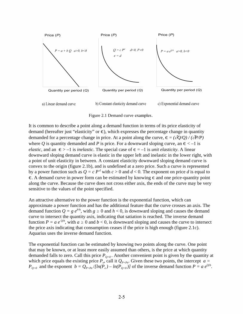
Demand functions are not easily estimated from market data. At any one time, all that isobserved is one point along the demand function–one price-quantity combination among a largenumber of combinations that could be observed under different conditions. However, by varioustechniques, including observation of different real-world or experimental markets involvingsimilar people in different supply situations, economists have learned about demand functions.Typically they find that as the price decreases the quantity consumed increases, yielding adownward sloping demand curve (figure 2.1). Further, although it is common in economics textbooks to illustrate demand functions using straight lines (figure 2.1a), most actual marketdemand functions are probably nonlinear. Of course, short portions of any demand curve can beapproximated by a straight line.

2-5

Figure 2.1 Demand curve examples.

It is common to describe a point along a demand function in terms of its price elasticity ofdemand (hereafter just “elasticity” or ,), which expresses the percentage change in quantitydemanded for a percentage change in price. At a point along the curve, , = (MQ/Q) / (MP/P)where Q is quantity demanded and P is price. For a downward sloping curve, an , < –1 iselastic, and an , > –1 is inelastic. The special case of , = –1 is unit elasticity. A lineardownward sloping demand curve is elastic in the upper left and inelastic in the lower right, witha point of unit elasticity in between. A constant elasticity downward sloping demand curve isconvex to the origin (figure 2.1b), and is undefined at a zero price. Such a curve is representedby a power function such as Q = c P d with c > 0 and d < 0. The exponent on price d is equal to,. A demand curve in power form can be estimated by knowing , and one price-quantity pointalong the curve. Because the curve does not cross either axis, the ends of the curve may be verysensitive to the values of the point specified.

An attractive alternative to the power function is the exponential function, which canapproximate a power function and has the additional feature that the curve crosses an axis. Thedemand function Q = g eP/h, with g $ 0 and h < 0, is downward sloping and causes the demandcurve to intersect the quantity axis, indicating that satiation is reached. The inverse demandfunction P = a e Q/b, with a $ 0 and b < 0, is downward sloping and causes the curve to intersectthe price axis indicating that consumption ceases if the price is high enough (figure 2.1c).Aquarius uses the inverse demand function.

The exponential function can be estimated by knowing two points along the curve. One pointthat may be known, or at least more easily assumed than others, is the price at which quantitydemanded falls to zero. Call this price PQ=0 . Another convenient point is given by the quantity atwhich price equals the existing price Pe, call it QP=Pe. Given these two points, the intercept a =PQ=0 and the exponent b = QP=Pe /[ln(Pe ) – ln(PQ=0 )] of the inverse demand function P = a eQ/b.

2-6

The two-point approach to estimating an exponential function fails to use information aboutelasticity of demand that may be available for at least one point along the demand curve.Elasticity varies along an exponential function. Aquarius includes a computational tool toestimate the coefficients of the exponential function knowing two points and the elasticity at oneof those two points. The tool uses a weighted least-square method to minimize the sum ofsquares of deviations of the observed points and elasticity from those of the fitted function. SeeAppendix B for details.

The coefficient b of the exponent in the inverse demand function P = a e Q/b is negative if thecurve is downward sloping. However, note that when specifying b in Aquarius the minus sign isassumed, so that the user enters only the absolute value of b (i.e., P = a e -Q/b) (see Chapter 4 andAppendix B).

It is important to distinguish between demand for water in general and demand for water fromthe particular source being modeled. For example, demand for the first increments of residentialwater is extremely high. Thus, a demand curve for residential water in general might intersectthe price axis at a very high price. However, residential water from a particular source may havealternative, though more costly, sources. The cost of the next more costly source would truncatethe demand curve for the particular source at issue at a price equal to that cost. Whenever analternative source exists, its cost can serve as an estimate of PQ=0.

When comparing demand functions for water in different uses it is important that each demandfunction be for raw water. For example, it would be incorrect to compare demand for raw waterin irrigation with demand for treated and delivered water in residential use. The latter estimate ofwillingness to pay would include the cost of treatment and delivery whereas the former wouldnot. If the process of estimating a demand function for a particular water use focuses on treatedand delivered water, treatment and delivery costs must be removed from the estimatedwillingness to pay to yield demand for raw water.

For offstream water uses that do not completely consume the diverted water, such as mostagricultural and municipal withdrawals, the quantity variable in a water demand function must bechosen to correspond with the way diversions are being modeled. Sometimes in modeling waterallocation, only the consumptive use amount is modeled; that is, withdrawal is set equal to theconsumptive use and return flow is thereby ignored. This is a viable procedure if actual return flowsreach the stream upstream of the next downstream diversion point of the model. In this case,consumptive use is the appropriate quantity variable for the water demand function. A moreaccurate characterization of water movement in a river basin is achieved by explicitly modelingreturn flows and specifying the point where they reach the water course. In this case, withdrawal isthe appropriate quantity variable. Either way, consumptive use includes actual evapotranspiration atthe location of use plus any other losses along the delivery and return paths.

In a well functioning water market, the marginal value of raw water is equal across uses. Thisequality occurs because, if marginal values differ, the higher-valued use can afford to purchasewater from a lower-valued use, paying a price that exceeds the water's value in the lower-valueduse. Transfers from lower-valued to higher-valued uses continue until the advantages of trade areeliminated, that is, until marginal values are equal and an optimal allocation is reached. Equalityof value at the margin does not indicate equality of value over the full extent of the demand

2-7

curve. Indeed, the value of the initial units of water to domestic or industrial uses, for example, isgreater than the value of initial units to most irrigated agriculture. However, in the absence ofinstitutional barriers to trade or significant transaction costs, actual marginal raw water deliveriesto each water use will occur at the point of equal marginal value.

Markets in the real world rarely perform as smoothly as they do in theory. Water transfers areoften constrained by institutional barriers such as contractual agreements attached to publiclyfunded storage and delivery projects that preclude sale to unauthorized uses, or by the lack oflegal recognition of some water uses such as habitat maintenance. Water transfers are alsotypically impeded by significant transaction costs such as those associated with quantifying andlegally defending return flow amounts. Institutional barriers and transaction costs may keepmarginal values of water in different uses from reaching equality, requiring separate valuationefforts to estimate the current marginal values of water in different uses.

In the following sections, we present information that will facilitate use of Aquarius including:1) evidence on the shape of the annual demand curve; 2) detail on placing the annual demandcurve in realistic price-quantity space; 3) information on the difference between demand fortreated and delivered water and demand for raw water; and 4) information on disaggregatingannual demand to the monthly time step. Prices from studies performed over the past twentyyears or so are reported. We have, unless stated otherwise, adjusted for inflation by updatingthese prices to 1995 dollars using the Gross Domestic Product (GDP) implicit price deflator.

Irrigation Water Use

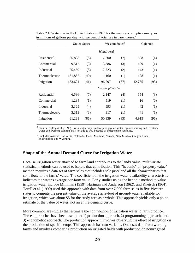
Irrigation in the United States in 1995 accounted for 41 percent of fresh water withdrawals and85 percent of consumptive use (table 2.1). In the 11 most western contiguous states, 87 percentof withdrawals and 93 percent of consumptive use was for agriculture. In some states, such asColorado, irrigation plays an even more important role (table 2.1).

The most direct approach to estimating the demand for irrigation water is to observe markettransactions where water rights are purchased by farmers in a competitive water market. Suchtransactions, however, seldom occur. Although farmers in some parts of the West commonly sellwater rights to municipal and industrial water users, and sometimes do so in relatively competitivemarkets, instances of open market water purchase by farmers are uncommon (Brown 2004).

Lacking a direct measure of farmers' demand for irrigation water, economists have focused onwater's role as an agricultural input. This role affects two end products that are commonly sold incompetitive markets; farm land and farm produce. Thus, water demand schedules are derived byestimating the contribution of irrigation water towards either the value of irrigated farms or thevalue of farm produce. The viability of these approaches rests on the degree to which the endproducts and non-water inputs are competitively priced. Subsidies and other impediments to thefree working of markets can alter prices to such an extent that the estimated water price reflectsmarket manipulation or control rather than resource demand and scarcity. Although thecompetitive market requirements are rarely met completely, they have been met to a sufficientdegree to sustain, over the past 40 years or so, numerous studies of the value irrigation water.

2-8

Table 2.1 Water use in the United States in 1995 for the major consumptive use types in millions of gallons per day, with percent of total use in parentheses.a

United States Western Statesb Colorado

Withdrawal

Residential 25,888 (8) 7,200 (7) 508 (4)

Commercial 9,512 (3) 3,386 (3) 109 (1)

Industrial 25,459 (8) 2,723 (2) 143 (1)

Thermoelectric 131,852 (40) 1,160 (1) 128 (1)

Irrigation 133,621 (41) 96,297 (87) 12,735 (93)

Consumptive Use

Residential 6,596 (7) 2,147 (4) 154 (3)

Commercial 1,294 (1) 519 (1) 16 (0)

Industrial 3,365 (4) 593 (1) 42 (1)

Thermoelectric 3,313 (3) 317 (1) 41 (1)

Irrigation 81,231 (85) 50,939 (93) 4,915 (95)

a Source: Solley et al. (1998). Fresh water only, surface plus ground water. Ignores mining and livestock water use. Percent columns may not add to 100 because of independent rounding. b Includes Arizona, California, Colorado, Idaho, Montana, Nevada, New Mexico, Oregon, Utah, Washington, and Wyoming.

Shape of the Annual Demand Curve for Irrigation Water

Because irrigation water attached to farm land contributes to the land's value, multivariatestatistical methods can be used to isolate that contribution. This "hedonic" or "property value"method requires a data set of farm sales that includes sale price and all the characteristics thatcontribute to the farms’ value. The coefficient on the irrigation water availability characteristicindicates the water's average per-farm value. Early studies using the hedonic method to valueirrigation water include Milliman (1959), Hartman and Anderson (1962), and Knetsch (1964).Torell et al. (1990) used this approach with data from over 7,000 farm sales in five Westernstates to compute the present value of the average acre-foot of ground-water available forirrigation, which was about $5 for the study area as a whole. This approach yields only a pointestimate of the value of water, not an entire demand curve. More common are studies that estimate the contribution of irrigation water to farm produce.Three approaches have been used, the: 1) production approach, 2) programming approach, and3) econometric approach. The production approach involves observing the effect of irrigation onthe production of specific crops. This approach has two variants. One uses data from workingfarms and involves comparing production on irrigated fields with production on nonirrigated

2-9

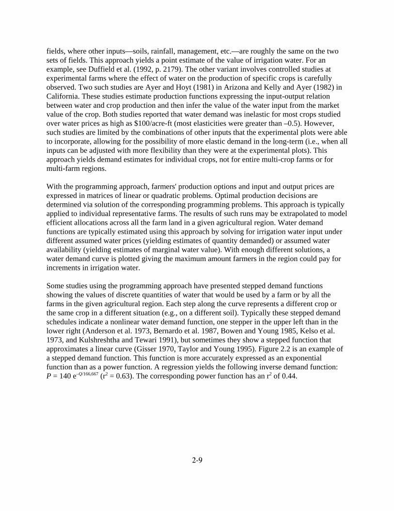
fields, where other inputs—soils, rainfall, management, etc.—are roughly the same on the twosets of fields. This approach yields a point estimate of the value of irrigation water. For anexample, see Duffield et al. (1992, p. 2179). The other variant involves controlled studies atexperimental farms where the effect of water on the production of specific crops is carefullyobserved. Two such studies are Ayer and Hoyt (1981) in Arizona and Kelly and Ayer (1982) inCalifornia. These studies estimate production functions expressing the input-output relationbetween water and crop production and then infer the value of the water input from the marketvalue of the crop. Both studies reported that water demand was inelastic for most crops studiedover water prices as high as $100/acre-ft (most elasticities were greater than –0.5). However,such studies are limited by the combinations of other inputs that the experimental plots were ableto incorporate, allowing for the possibility of more elastic demand in the long-term (i.e., when allinputs can be adjusted with more flexibility than they were at the experimental plots). Thisapproach yields demand estimates for individual crops, not for entire multi-crop farms or formulti-farm regions.

With the programming approach, farmers' production options and input and output prices areexpressed in matrices of linear or quadratic problems. Optimal production decisions aredetermined via solution of the corresponding programming problems. This approach is typicallyapplied to individual representative farms. The results of such runs may be extrapolated to modelefficient allocations across all the farm land in a given agricultural region. Water demandfunctions are typically estimated using this approach by solving for irrigation water input underdifferent assumed water prices (yielding estimates of quantity demanded) or assumed wateravailability (yielding estimates of marginal water value). With enough different solutions, awater demand curve is plotted giving the maximum amount farmers in the region could pay forincrements in irrigation water.

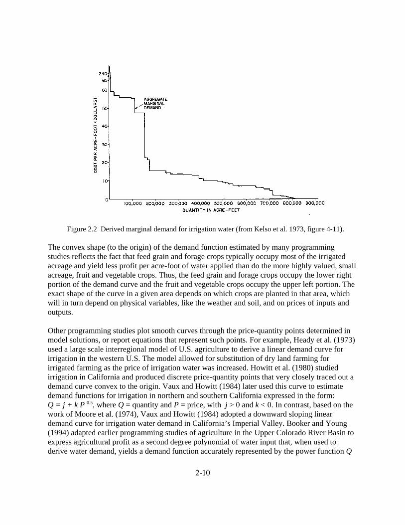
Some studies using the programming approach have presented stepped demand functionsshowing the values of discrete quantities of water that would be used by a farm or by all thefarms in the given agricultural region. Each step along the curve represents a different crop orthe same crop in a different situation (e.g., on a different soil). Typically these stepped demandschedules indicate a nonlinear water demand function, one stepper in the upper left than in thelower right (Anderson et al. 1973, Bernardo et al. 1987, Bowen and Young 1985, Kelso et al.1973, and Kulshreshtha and Tewari 1991), but sometimes they show a stepped function thatapproximates a linear curve (Gisser 1970, Taylor and Young 1995). Figure 2.2 is an example ofa stepped demand function. This function is more accurately expressed as an exponentialfunction than as a power function. A regression yields the following inverse demand function: P = 140 e–Q/166,667 (r2 = 0.63). The corresponding power function has an r2 of 0.44.

2-10

Figure 2.2 Derived marginal demand for irrigation water (from Kelso et al. 1973, figure 4-11).

The convex shape (to the origin) of the demand function estimated by many programmingstudies reflects the fact that feed grain and forage crops typically occupy most of the irrigatedacreage and yield less profit per acre-foot of water applied than do the more highly valued, smallacreage, fruit and vegetable crops. Thus, the feed grain and forage crops occupy the lower rightportion of the demand curve and the fruit and vegetable crops occupy the upper left portion. Theexact shape of the curve in a given area depends on which crops are planted in that area, whichwill in turn depend on physical variables, like the weather and soil, and on prices of inputs andoutputs.

Other programming studies plot smooth curves through the price-quantity points determined inmodel solutions, or report equations that represent such points. For example, Heady et al. (1973)used a large scale interregional model of U.S. agriculture to derive a linear demand curve forirrigation in the western U.S. The model allowed for substitution of dry land farming forirrigated farming as the price of irrigation water was increased. Howitt et al. (1980) studiedirrigation in California and produced discrete price-quantity points that very closely traced out ademand curve convex to the origin. Vaux and Howitt (1984) later used this curve to estimatedemand functions for irrigation in northern and southern California expressed in the form: Q = j + k P 0.5, where Q = quantity and P = price, with j > 0 and k < 0. In contrast, based on thework of Moore et al. (1974), Vaux and Howitt (1984) adopted a downward sloping lineardemand curve for irrigation water demand in California’s Imperial Valley. Booker and Young(1994) adapted earlier programming studies of agriculture in the Upper Colorado River Basin toexpress agricultural profit as a second degree polynomial of water input that, when used toderive water demand, yields a demand function accurately represented by the power function Q

2-11

= c P –0.66, with c > 0. The Vaux and Howitt (1984) and Booker and Young (1994) studies bothshowed downward sloping demand functions that were convex to the origin.

The econometric approach has been applied with cross-sectional data representing a largegeographical area over which water costs, perhaps because of pumping depths or applicationrates, vary substantially. For example, studies by Moore et al. (1994), Ogg and Gollehon (1989),and Frank and Beattie (1979) each used data from several western U.S. states. Ogg and Gollehonregressed water use on water price variables using three different functional forms. The mostsuccessful model used a power function, yielding an irrigation water demand function that isconvex to the origin, with a constant elasticity of –0.26. Frank and Beattie assumed a powerfunction and regressed the value of agricultural production on a set of explanatory variables.They found elasticities of demand for irrigation water from –1.0 to –1.5 depending on thegeographical region. Using data from seven Texas counties, Nieswiadomy (1985) regressedgroundwater pumping on explanatory variables including pumping cost and compared linear andlog-log (i.e., power) functional forms. The functional forms differed little in their ability toexplain variance in the pumping rate. The log-log coefficient on pump cost, equivalent to theelasticity of demand, was –0.8.

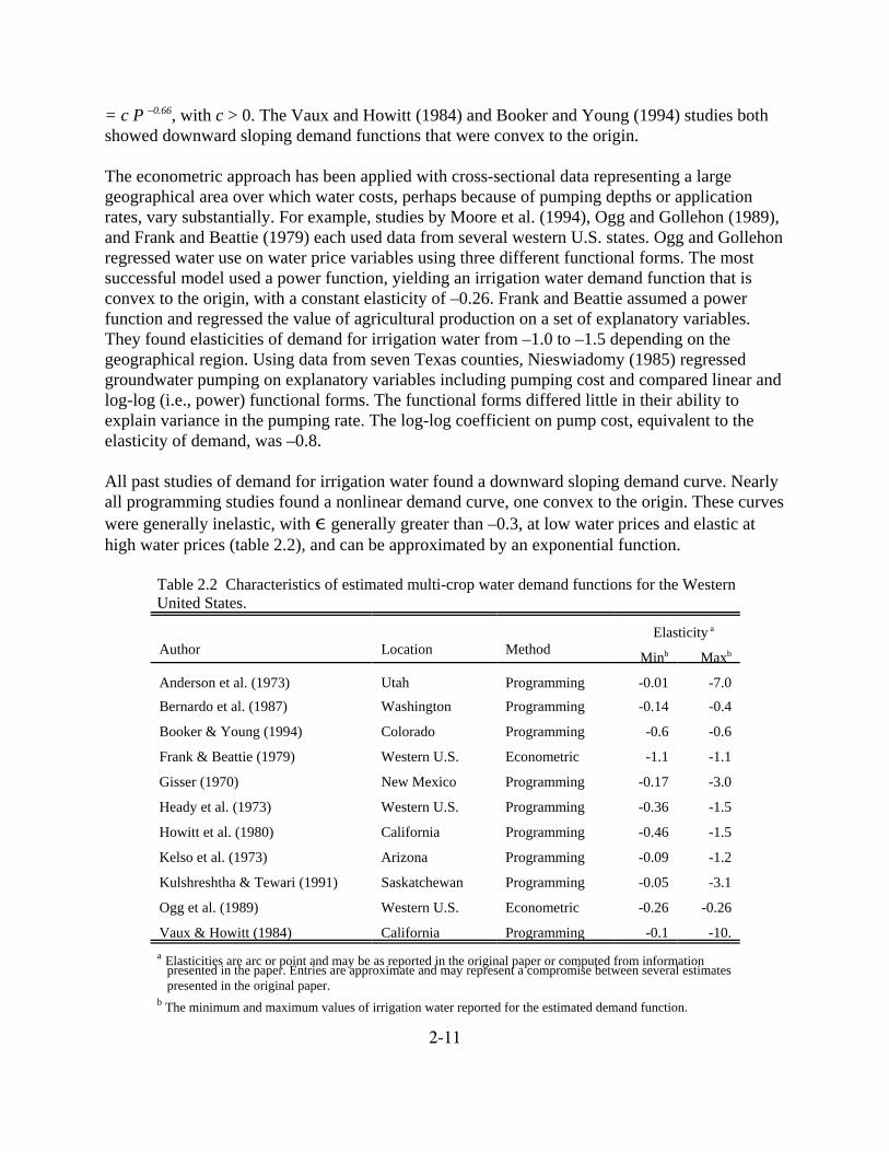
All past studies of demand for irrigation water found a downward sloping demand curve. Nearlyall programming studies found a nonlinear demand curve, one convex to the origin. These curveswere generally inelastic, with , generally greater than –0.3, at low water prices and elastic athigh water prices (table 2.2), and can be approximated by an exponential function.

Table 2.2 Characteristics of estimated multi-crop water demand functions for the Western United States.

Author Location Method Elasticity a

Minb Maxb

Anderson et al. (1973) Utah Programming -0.01 -7.0Bernardo et al. (1987) Washington Programming -0.14 -0.4

Booker & Young (1994) Colorado Programming -0.6 -0.6

Frank & Beattie (1979) Western U.S. Econometric -1.1 -1.1

Gisser (1970) New Mexico Programming -0.17 -3.0

Heady et al. (1973) Western U.S. Programming -0.36 -1.5

Howitt et al. (1980) California Programming -0.46 -1.5

Kelso et al. (1973) Arizona Programming -0.09 -1.2

Kulshreshtha & Tewari (1991) Saskatchewan Programming -0.05 -3.1

Ogg et al. (1989) Western U.S. Econometric -0.26 -0.26

Vaux & Howitt (1984) California Programming -0.1 -10.a Elasticities are arc or point and may be as reported in the original paper or computed from information presented in the paper. Entries are approximate and may represent a compromise between several estimates presented in the original paper.b The minimum and maximum values of irrigation water reported for the estimated demand function.

2-12

Of the studies that fitted smooth curves to these results, Vaux and Howitt (1984) used nonlinearand linear functions and Booker and Young (1994) presented a profit function that yielded a demandfunction that we most accurately expressed in an equation in power form. The econometric studiesgenerally either assume a power function—a common practice in economic studies partly becausethe exponent on price in a demand function is equal to the price elasticity—or find upon comparisonthat such a function performs better in terms of explained variance.

Representative Annual Irrigation Water Demand Curve

The amount of irrigation water diverted in a given farming area depends on many factors. Ifwater is not limited it will be diverted up to the point where its marginal value equals thefarmer's marginal cost of acquiring and applying the water. Where water limitations keepirrigation below the level at which marginal value equals marginal cost, the demand curve istruncated by the resource constraint. In any case, as the price of water increases, water use peracre may drop somewhat, but the main change will probably be a reduction in the number ofacres irrigated as acres are converted to dry land crops or removed from production. Therefore,the quantity axis of the demand curve cannot be expressed on a quantity per-acre basis, unlikethe demand curve for residential water, which can be expressed on a quantity per-capita basis, asevery person needs some water. The appropriate variable for the quantity axis of the irrigationdemand curve is water volume per year for the entire agricultural area.

Ideally, the demand curve for the agricultural area(s) to be included in a river basin waterallocation model should be carefully derived. However, where a demand curve has not beenderived, an approximation can be achieved by adopting a functional form and knowing one ortwo points along the curve. Assuming an exponential form, two points are needed such as PQ=0and QP=Pe. To provide rough estimates of these points, various papers were examined. The pricesat the upper left of the demand curves (approximating PQ=0) varied from under $100 to over$200/acre-ft. The estimated maximum prices depend on whether high-value fruits and vegetablesare grown in the area. The quantity demanded at the existing marginal price (QP=Pe) will varywith the acreage available for planting, soil type, weather (principally temperature andprecipitation), method of application (flood versus spray), etc. Existing prices are typically from$5 to $15/acre-ft for surface water delivered via gravity but may vary more widely if pumped.The following studies reported ground water pumping costs: Ogg and Gollehon (1989) describedcosts from $54 to $102/acre-ft across the West; Moore et al. (1994) reported costs ranging from$25 to $32 across the West; and Nieswiadomy (1985) related a cost of about $7 for areas ofTexas. These prices should correspond to withdrawals per acre across the West that, according toSolley et al. (1998, table 15), vary from 1.45 acre-ft on average in the Texas-Gulf region to 5.71acre-ft on average in the Lower Colorado region. For comparison, the weighted mean fresh wateragricultural withdrawal over the nine Western water resource regions was 2.90 acre-ft/acre(Solley et al. 1998).

2-13

Because there is considerable variety across the West, some knowledge of local conditions isneeded to estimate PQ=0, Pe and QP=Pe. But to provide an example, assume an exponentialfunctional form, where PQ=0 = $150, Pe = $15, an irrigated area of 10,000 acres, and existingannual withdrawals of 3 acre-ft/acre. Using these assumptions, the annual inverse demandfunction is P = 150 e–Q/13,000.

Demand for Raw Water

The cost of irrigating crops includes the expense of delivering water to the farm and applying itto the crops. Demand for raw water is estimated net of delivery and application costs. Oneapproach to estimating the demand curve for raw water is to subtract delivery and applicationcosts from willingness to pay for delivered and applied water.

Delivery costs for gravity-fed water are mainly the expense of constructing, maintaining, andoperating dams and canals. In most gravity-fed irrigation areas, these functions are performed byan association, such as an irrigation district, which, to cover the association's costs, chargesindividual farmers a fixed assessment fee per unit of water owned. Thus, the assessment feeapproximates the amortized average cost of storing and delivering the water. Such fees typicallyvary from $5 to $20/acre-ft. (A further complication, when evaluating economic efficiency, isthe effect of government subsidies on the values of agricultural products and the costs ofagricultural inputs. Many of the West's dams and canal systems have been publicly subsidized tosome extent.) Delivery costs for pumped water consist largely of the pumping expense.Marginal pumping cost is a function of energy unit cost and pumping depth, which are typicallyrather constant per acre-foot for an individual farmer in a given year.

Application costs vary by method. These costs may include fixed costs, such as for fieldleveling, installing ditches, and installing sprinkler equipment, and variable costs such as forhand moving of syphons or sprinkler heads and maintaining ditches or sprinkler equipment.

Monthly Distribution of Annual Demand

Farmers make water use decisions at various times. In the long run, all factors of productionunder the farmer’s control are variable. For example, the choice of whether to install a sprinkleirrigation system is variable in the long run. Annual (intermediate run) decisions focus largely onwhat to plant given expected prices and water availability. Monthly (short run) decisions usuallyfocus on responding to recent changes in prices and weather patterns. Daily (very short run)decisions might focus on how much water to apply to a specific field given existing moistureconditions. Decisions about the purchase of water rights or drilling a well are long orintermediate run decisions; decisions about rental of a water right (i.e., purchase of water forone-time use) are intermediate- or short-run decisions; and decisions about when to irrigate areshort-run or very short-run decisions.

2-14

Figure 2.3 Disaggregation of an annual demand curve.

Colorado Basinb

Upper Lower

January 0 4

February 0 7

March 0 9

April 4 10

May 23 10

June 35 11

July 23 12

August 12 11

September 3 9

October 0 7

November 0 5

December 0 4 a Source: U.S. Bureau of Reclamation (1986). b Columns may not sum to 100 because of rounding.

Table 2.3 Monthly allocation of annual irrigation withdrawals (in percent). a

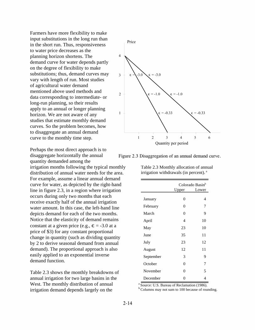
Farmers have more flexibility to makeinput substitutions in the long run thanin the short run. Thus, responsivenessto water price decreases as theplanning horizon shortens. Thedemand curve for water depends partlyon the degree of flexibility to makesubstitutions; thus, demand curves mayvary with length of run. Most studiesof agricultural water demandmentioned above used methods anddata corresponding to intermediate- orlong-run planning, so their resultsapply to an annual or longer planninghorizon. We are not aware of anystudies that estimate monthly demandcurves. So the problem becomes, howto disaggregate an annual demandcurve to the monthly time step.

Perhaps the most direct approach is todisaggregate horizontally the annualquantity demanded among theirrigation months following the typical monthlydistribution of annual water needs for the area.For example, assume a linear annual demandcurve for water, as depicted by the right-handline in figure 2.3, in a region where irrigationoccurs during only two months that eachreceive exactly half of the annual irrigationwater amount. In this case, the left-hand linedepicts demand for each of the two months.Notice that the elasticity of demand remainsconstant at a given price (e.g., , = -3.0 at aprice of $3) for any constant proportionalchange in quantity (such as dividing quantityby 2 to derive seasonal demand from annualdemand). The proportional approach is alsoeasily applied to an exponential inversedemand function.

Table 2.3 shows the monthly breakdowns ofannual irrigation for two large basins in theWest. The monthly distribution of annualirrigation demand depends largely on the

2-15

weather and on whether double cropping is practiced, which also depends on the weather. Astable 2.3 indicates, irrigated farming occurs year-round in the Lower Colorado Basin, whichincludes the desert areas of Arizona and California but not the cooler Upper Basin.

A limitation of the proportional approach is that it holds the maximum price, which is theintersection at the price axis, constant for all months at the level set by the annual demand curve,when in fact the farmer might be willing to pay more or less in some months. For example,because in a given month flexibility is limited to substitute among inputs, a farmer might bewilling to pay more for initial water quantities than the annual demand curve indicates. Anotherlimitation is that the assumption of constant monthly proportions of annual water use precludesthe possibility of adjusting the use among months in response to existing moisture conditions.Nevertheless, given the lack of estimated monthly demand functions and of data on howirrigation responds to natural moisture changes, the constant proportion disaggregation approachis probably the most viable.

Municipal Water Use

Distinctions among types of municipal and industrial (M&I) uses are unclear in the economicliterature. Some studies of "residential" or "domestic" demand use data from a sample ofindividual households and are clearly residential demand studies. Others use aggregated datafrom water providers that include deliveries to commercial, and possibly some industrial users,although the bulk of the deliveries are to residential users. In these studies, the terms"community", "municipal" and "residential" are often used inconsistently. In the followingsubsections on residential water use, "residential" and "municipal" studies are listed together andresults for the "municipal" studies that did not present separate estimates for residential andnonresidential users reflect the combination of residential and nonresidential uses. Commercialuse is presented separately. Industrial use is covered in the next section.

Residential water use in the U.S. is 7 percent of the total water withdrawal; commercial wateruse is an additional 2 percent. In relatively dry states with large agricultural sectors, such asColorado, these percentages are even lower (table 2.1). Although small in terms of quantity,municipal water use looms large in terms of average value per unit.

Shape of the Annual Demand Curve for Residential Water

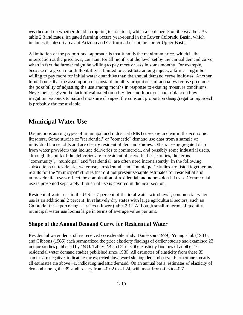
Residential water demand has received considerable study. Danielson (1979), Young et al. (1983),and Gibbons (1986) each summarized the price elasticity findings of earlier studies and examined 23unique studies published by 1980. Tables 2.4 and 2.5 list the elasticity findings of another 16residential water demand studies published since 1980. All estimates of elasticity from these 39studies are negative, indicating the expected downward sloping demand curve. Furthermore, nearlyall estimates are above –1, indicating inelastic demand. On an annual basis, estimates of elasticity ofdemand among the 39 studies vary from –0.02 to –1.24, with most from –0.3 to –0.7.

2-16

Table 2.4 Price elasticity of annual demand for residential water.a

Author Location Elasticity

Billings (1990) Tucson, AZ -0.57

Griffin (1990) Texas -0.37

Hanke & de Mare (1984) Malmo, Sweden -0.15

Jones & Morris (1984) Denver, CO -0.14 to -0.44

Martin & Thomas (1986) 5 cities in arid areas -0.49

Nieswiadomy (1992) Northeastern U.S. -0.28

Southern U.S. -0.60

Western U.S. -0.45

Rizaiza (1991) Saudi Arabia (4 cities) -0.40, -0.78

Schneider et al. (1991) Columbus, OH -0.26 to -0.50

Stevens et al. (1992) Massachusetts -0.41 to -0.69

Williams & Suh (1986) United States -0.49

a In most cases, the elasticities were estimated from a constant-elasticity functional form. Where avariable-elasticity functional form was used, we report the arc or point elasticity that was reportedin the original, which is estimated at the average price for the sample. A range is also listed ifdifferent estimation procedures or different conditions resulted in more than one estimate. Whereboth long- and short-run elasticities were reported, only the long-run elasticities are listed. Griffin(1990), Hanke and de Mare (1984), and the -0.5 estimate of Schneider et al. (1990) were listed as"municipal;" all others were listed as "residential."

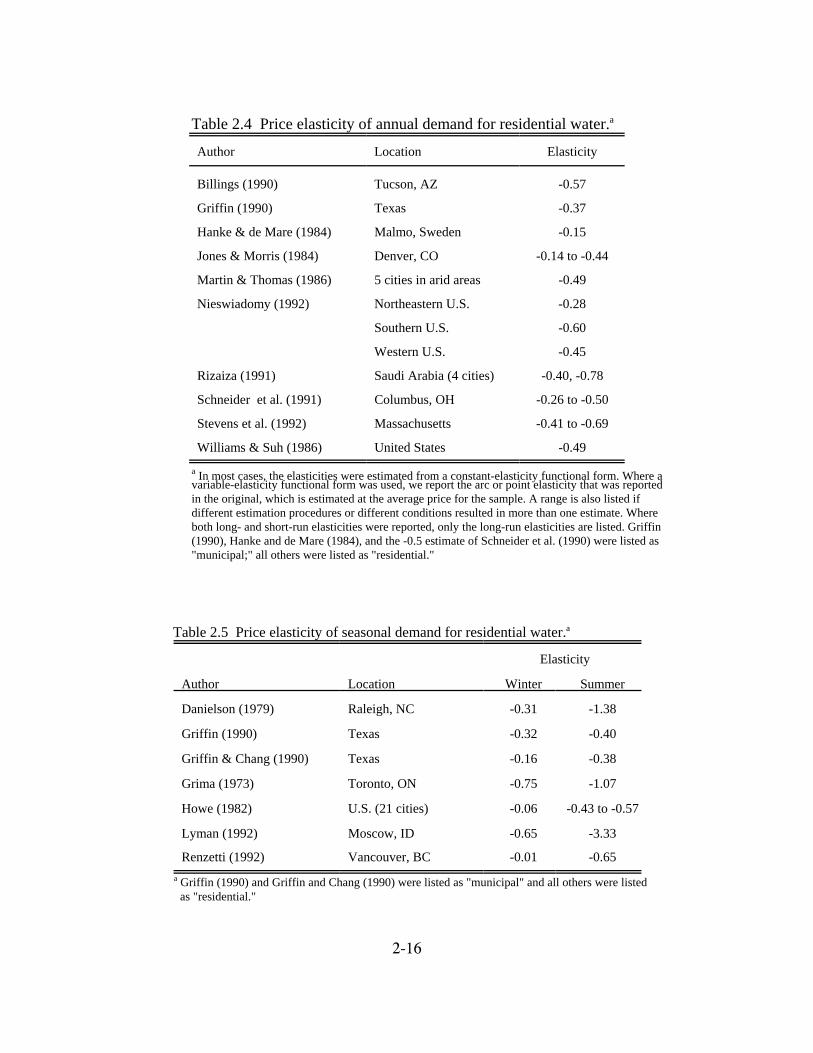
Table 2.5 Price elasticity of seasonal demand for residential water.a

Elasticity

Author Location Winter Summer

Danielson (1979) Raleigh, NC -0.31 -1.38

Griffin (1990) Texas -0.32 -0.40

Griffin & Chang (1990) Texas -0.16 -0.38

Grima (1973) Toronto, ON -0.75 -1.07

Howe (1982) U.S. (21 cities) -0.06 -0.43 to -0.57

Lyman (1992) Moscow, ID -0.65 -3.33

Renzetti (1992) Vancouver, BC -0.01 -0.65

a Griffin (1990) and Griffin and Chang (1990) were listed as "municipal" and all others were listed as "residential."

2-17

The estimates of elasticity among the 39 studies include a mixture from short-run to long-runestimates. Although most studies of water demand elasticity did not attempt to measure bothshort- and long-run elasticities, a few studies (e.g., Schneider et al. 1991, Lyman 1992) estimatedboth and found that long-run demand is more elastic than short-run demand. This difference inelasticity reflects adaptations to changing prices that occur gradually as consumers change habitsand alter water using appliances or landscape vegetation.

Nearly all studies of residential or municipal water demand use an econometric approach, mostwith cross-sectional data but some with time series data. Most studies assume a non-linearfunctional form, thereby predetermining the shape of the annual demand curve. Many studiesassume a Cobb-Douglas (power) function that yields a constant elasticity curve; note the numberof studies listed in table 2.4 with only one elasticity estimate, which indicates a constantelasticity model. Some other studies (e.g., Foster and Beattie 1979) assume an exponentialfunction on water price.

Studies of water demand in the U.S., whether cross-sectional or time-series studies, have useddata with relatively little variation in water price. For example, average prices charged by the218 cities studied by Foster and Beattie (1979) varied across cities from $0.10 to $1.79/m3, andaverage prices charged by the 30 Texas communities studied by Griffin and Chang (1990) variedacross communities from $0.34 to $1.62/m3. U.S. studies do not include cases with sufficientlyhigh water prices to allow accurate estimates of the shape of the upper left portion of the demandcurve. Thus, the estimates of price elasticity reported in the 39 studies apply to the low-priceportion of the residential demand curve.

Martin and Thomas (1986) provided a unique estimate of the entire demand curve for residentialwater via their comparison of water use in five cities that, although sharing an arid climate, differmarkedly in the cost of providing water and in the price charged to consumers. These prices variedfrom $0.16 to $25.01/m3 and represent cities in the U.S., Kuwait, and Australia (table 2.6).

Table 2.6 Residential water price and quantity data for selected cities.

Author LocationQuantity

(l/c/d)aPrice

($/m3)b

Martin & Thomas (1986)c Coober Pedy, Australiad 50 25.01

Kuwait urban areas 184 1.19

Perth, Australia 288 0.55

Tucson, AZ 371 0.48

Phoenix, AZ 595 0.16

Rizaiza (1991)e Taif, Saudi Arabia 35 8.39

a Liters per capita per day. b 1995 dollars. c Marginal prices. d Desalinized water delivered by tanker. e Average prices. Delivered by tanker.

2-18

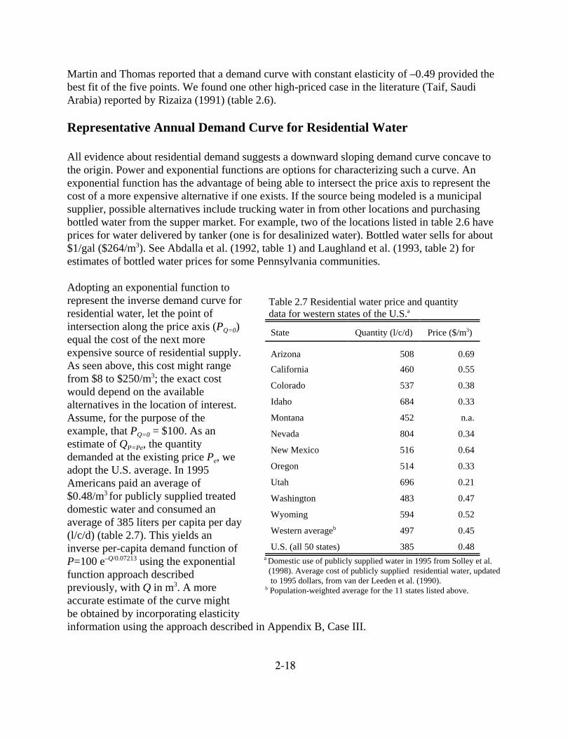
Table 2.7 Residential water price and quantity data for western states of the U.S.a

State Quantity (l/c/d) Price ($/m3)

Arizona 508 0.69California 460 0.55

Colorado 537 0.38

Idaho 684 0.33

Montana 452 n.a.

Nevada 804 0.34

New Mexico 516 0.64

Oregon 514 0.33

Utah 696 0.21

Washington 483 0.47

Wyoming 594 0.52

Western averageb 497 0.45

U.S. (all 50 states) 385 0.48 a Domestic use of publicly supplied water in 1995 from Solley et al. (1998). Average cost of publicly supplied residential water, updated to 1995 dollars, from van der Leeden et al. (1990). b Population-weighted average for the 11 states listed above.

Martin and Thomas reported that a demand curve with constant elasticity of –0.49 provided thebest fit of the five points. We found one other high-priced case in the literature (Taif, SaudiArabia) reported by Rizaiza (1991) (table 2.6).

Representative Annual Demand Curve for Residential Water

All evidence about residential demand suggests a downward sloping demand curve concave tothe origin. Power and exponential functions are options for characterizing such a curve. Anexponential function has the advantage of being able to intersect the price axis to represent thecost of a more expensive alternative if one exists. If the source being modeled is a municipalsupplier, possible alternatives include trucking water in from other locations and purchasingbottled water from the supper market. For example, two of the locations listed in table 2.6 haveprices for water delivered by tanker (one is for desalinized water). Bottled water sells for about$1/gal ($264/m3). See Abdalla et al. (1992, table 1) and Laughland et al. (1993, table 2) forestimates of bottled water prices for some Pennsylvania communities.

Adopting an exponential function torepresent the inverse demand curve forresidential water, let the point ofintersection along the price axis (PQ=0)equal the cost of the next moreexpensive source of residential supply.As seen above, this cost might rangefrom $8 to $250/m3; the exact costwould depend on the availablealternatives in the location of interest.Assume, for the purpose of theexample, that PQ=0 = $100. As anestimate of QP=Pe, the quantitydemanded at the existing price Pe, weadopt the U.S. average. In 1995Americans paid an average of$0.48/m3 for publicly supplied treateddomestic water and consumed anaverage of 385 liters per capita per day(l/c/d) (table 2.7). This yields aninverse per-capita demand function of P=100 e–Q/0.07213 using the exponentialfunction approach describedpreviously, with Q in m3. A moreaccurate estimate of the curve mightbe obtained by incorporating elasticityinformation using the approach described in Appendix B, Case III.

2-19

Commercial Water Use

Few studies have estimated demand for commercial water uses. Table 2.8 lists three of the availablestudies. One of these studies, by Schnieder et al. (1991), separated government and school use fromother commercial uses. Schneider et al. also estimated residential demand and concluded thatcommercial demand was much more elastic than residential demand. This conclusion is sensitive tothe particular kinds of commercial establishments included in their data. Lynne et al. (1978)estimated demand for numerous types of commercial establishments (e.g., motels and departmentstores) and found a wide range in price elasticity at existing water prices.

Given the small number of commercial water-use studies, the wide range in elasticity estimatesamong these studies, and the small variability in water price across studies, estimating arepresentative demand curve for commercial water is risky. An alternative is to estimate amunicipal demand curve representing the combination of residential and commercial use. This isbest done with municipal data. However, if only residential data are available, one can–withsome loss in accuracy–use the residential demand curve along with an adjustment for theadditional use per capita represented by commercial use. As seen in table 2.1, commercialwithdrawals tend to be about 30 percent of residential withdrawals.

Table 2.8 Price elasticity of annual demand for commercial and industrial water.

Author LocationType of water use Elasticity

Commercial Lynne et al. (1978) Miami, FL Commercial -0.11 to -1.33

Schneider et al. (1991) Columbus, OH Commercial -0.92

Government -0.78

School -0.96

Williams & Suh (1986) United States Commercial -0.36

Industrial

De Rooy (1974) New Jersey Industrial -0.35 to -0.89

Elliott (1973) 29 US cities Industrial -0.64

Grebenstein & Field (1979) United States Industrial -0.33 to -0.80

Renzetti (1992a) Vancouver, BC Industrial -1.91

Renzetti (1992b) Canada Industrial -0.15 to -0.59

Renzetti (1993) Canada Industrial -0.66 to -2.17

Schneider et al. (1991) Columbus, OH Industrial -0.44

Turnovsky (1969) 16 towns in MA Industrial -0.50

Williams & Suh (1986) United States Industrial -0.74

2-20

Table 2.9 Examples of monthly allocation of of annual municipal deliveries (in percent)a

Texascommunitiesb

Front Rangecommunitiesc

January 6.7 5.3

February 6.8 5.6

March 6.9 5.6

April 7.9 6.3

May 8.5 6.4

June 9.5 9.8

July 11.2 14.8

August 11.2 16.8

September 9.9 11.4

October 7.5 7.2

November 6.8 5.6

December 6.8 5.2 a Columns may not total 100 because of rounding.

b From Griffin (1990), based on data from 221 communities. Figures are for 1981-85. Average annual use was 629 l/c/d. c Weighted (by population) average 1995 deliveries of the following Colorado cities: Fort Collins, Loveland, Longmont, Greeley/Evans, Pueblo, and Denver. Average annual use in 1995 was 745 l/c/d.

Demand for Raw Water

The cost of treatment and delivery must be subtracted from the total payment to yield the rawwater value. The best generally available estimate of treatment and delivery costs is the averagecost of delivered municipal water, based on the reasoning that utilities providing water typicallyset rates to just cover their costs. As mentioned, the average U.S. cost is $0.48/m3 for publiclysupplied treated domestic water, but costs may vary considerably from one location to another(see table 2.7 for state averages). Assuming constant returns to scale, the cost is subtracted fromthe willingness to pay over the full range of quantity demanded to yield the demand curve forraw municipal water.

Monthly Distribution of Municipal Demand

Several studies found that residential demand elasticity differs by season, with elasticity beinggreater in summer than in winter (table 2.5). The principal difference between the seasons is thatoutdoor use, largely for lawn and garden watering, occurs in the warmer months. However,whereas winter elasticities are consistently below summer elasticities, there is little consistencyacross studies in the estimates of elasticity ineither season. Across the studies winterestimates range from –0.01 to –0.75 andsummer estimates range from –0.38 to –3.33(table 2.5). The wide range in elasticityestimates for a given season reflects, in part,climatic differences among the locationsstudied and methodological differences amongthe studies.

Table 2.9 gives monthly breakdowns of annualwater use for some comunities in Texas andalong the Colorado Front Range. The greaterconcentration of deliveries during the summermonths along the Front Range versus Texasreflects the difference in climate, withgenerally drier conditions found along theFront Range. Note that indoor water useremains quite constant throughout the year, butoutdoor use responds to weather, which variesfrom one year to the next. Thus the summerestimates in table 2.9 may not berepresentative of long-term averages.

As with irrigated agriculture, the most directapproach to specifying monthly demand curvesis to horizontally disaggregate annual water

2-21

demand based on the typical monthly proportions of annual water use. Because indoor water useis the most valuable portion of domestic use and does not vary with weather conditions, the pointwhere the monthly demand curve intersects the vertical axis should remain constant acrossmonths. The greater elasticity of demand (table 2.5) and greater quantity demanded (table 2.9) inthe summer months lead to a summer demand curve that stretches further to the right and isflatter at a given price than one of the winter months.

Industrial Water Use

Industrial water use in the U.S. is dominated by use in thermoelectric power generation (table 2.1).For the country as a whole, thermoelectric power generation accounts for 40 percent of totalwithdrawals, with other industrial uses accounting for an additional 8 percent. However, the relativeimportance of industry is considerably less in the West, where thermoelectric power generation andother industrial uses account for only 2 and 1 percent of total withdrawals, respectively.

The estimates of elasticity for industrial water use summarized in table 2.8 appear in aggregate tobe smaller (more elastic) than those for residential water (table 2.4). As with commercial uses,elasticity of demand for industrial uses varies among alternative types of industries (Renzetti1992b, 1993, De Rooy 1974). Thus, the elasticity of demand in any urban area would besensitive to the particular industries located there.

The cost of water is a very small part of total production costs in most industries (Bower 1966,Gibbons 1986), suggesting that industries might be able to pay considerable sums for water.However, because most industrial water users can recycle water in their production processes,they are unwilling to pay more for additional water withdrawals than the cost of installing orimproving a recycling capability. Thus, the value of marginal withdrawals is approximated bythe marginal cost of recycling. Gibbons (1986), citing Young and Gray (1972) and Russell(1970), reported marginal cost estimates of $9 to $20/acre-ft for cooling water and $91 to$134/acre-ft for industrial process water.

With complete recycling, withdrawal equals consumptive use. However, as seen in table 2.1, theindustrial sector in general is far from achieving complete recycling. Thus, the value ofwithdrawals should approximate the marginal cost of recycling for a substantial proportion of thetotal industrial withdrawal. However, as withdrawal amount approaches consumptive useamount, the value of industrial water use must increase substantially. When this occurs, thedemand curve for industrial water can be expected to rise sharply as quantity demandedapproaches consumptive use. This suggests a nonlinear demand curve, convex to the origin, ascould be depicted by a power or exponential function.

Unfortunately, specific estimates of an industrial water use demand curve are not generallyavailable in the literature. If industrial water use is significant in a basin where water allocationis being analyzed using a model like Aquarius, a site-specific study may be necessary.

2-22

Hydropower

As Young and Gray (1972) and Gibbons (1986) explain, the value of hydroelectric energy iscommonly estimated using the alternative cost technique, based on the reasoning that electricitynot produced at hydroelectric dams will be produced using the next more expensive process. Use of the alternative cost valuation method is appropriate because the energy produced at ahydroelectric plant typically enters a large electric grid, composed of many hydro and thermalelectric plants, that supplies numerous demand areas. The various plants in the grid aresubstitute suppliers. If one supplier reduces production, other suppliers make up the difference,and a small shift from hydro to a more expensive energy source will have a negligible effect onoverall energy prices. Typically, baseload power produced at a hydroelectric plant is replaced bya coal-fired plant and peaking power is replaced by a gas- or oil-fired turbine plant. In thewestern U.S., gas-fired turbines are most common. More expensive oil-fired turbines also playan important role in the eastern U.S.

Using the alternative cost method, the value of hydropower in dollars per acre-foot is estimatedto be equal to 0.87 × feet of head × cost savings, where the cost savings is the cost per kilowatthour (kWh) at thermal plants minus the cost per kilowatt hour at hydro plants. The 0.87 reflectsthe efficiency of converting the energy of falling water into electrical energy. The cost savingsmay be determined for the short run or long run. In t mhe short run, capital costs are fixed andthe only costs of note are those for operation and maintenance (O&M). At thermal plants, O&Mcosts are dominated by the cost of fuel. Variable costs tend to be constant per unit of output,allowing simple average costs to be used regardless of the quantity of electricity. Gibbons (1986)reported that O&M costs at U.S. thermal plants averaged 18.52 and 44.01 mills/kWh at coal-fired and gas-fired plants, respectively, whereas the O&M costs at private hydroelectric plantsaveraged 1.52 mills/kWh (1980 dollars). The short-run values of hydropower thus averaged$0.0148 and $0.0370/acre-ft per foot of head for baseload and peaking power, respectively.

Fuel prices are changeable. At about the time Gibbons (1986) published her report, the prices perkWh that electricity plants paid for fuel dropped, nationally to about 14 mills for coal and 23mills for natural gas (Energy Information Administration 1996). These lower prices by and largewere maintained for more than a decade. However, natural gas prices have recently (2004-2005)been rising dramatically; nationally, prices per kWh rose to over 60 mills for natural gas,although coal prices changed little. Price changes have corresponding effects on total O&M costsat thermal plants. Accurate estimates of the value of hydropower require careful examination ofcosts at the affected thermal plants, along with decisions about how to represent the long-runtrend in fuel prices given data on actual prices that may show considerable short-term variations.

A long-run value would take into account the full costs of both types of plants and would includecapital costs in addition to O&M costs. Estimating these costs is an involved process. Young andGray (1972) provided one attempt to estimate the long-run value of hydropower. As Gibbons(1986) indicated, in an update of Young and Gray's work, the long-run cost savings per kilowatthour may be smaller than the short-run cost savings. Most economic studies use short-run values.

2-23

Gibbons (1986) reminds us that using the alternative cost method described above ignores somecosts, such as the environmental costs of thermal plants (e.g., air pollution) and hydro plants(e.g., inundation of a riparian area), and ignores the differences in the reliability of servicebetween the two kinds of generating plants. However, similar costs of other water uses (e.g.,nonpoint source pollution in irrigated agriculture) are also typically ignored when estimatingwater value. Such costs should be separately accounted for if economic efficiency is at issue.

Water Demand Curve in Hydroelectric Energy Production

Because per-unit variable costs at thermal plants(which consist largely of fuel costs) tend to bequite constant, if the amount of energy produced at the hydro plant of interest makes a relativelysmall contribution to the electric grid, then demand for water at hydroelectric plants is aptlycharacterized by a horizontal demand curve. The point where this horizontal demand curveintersects the price axis depends on the relative costs of the hydroelectric plant and its least costsubstitute. As described earlier, this depends on whether the hydroelectric plant producespeaking or baseload energy or some combination of the two. The annual and monthly demandcurves would be identical except for their lengths, which indicate the capacities of the hydroplants for the respective time periods. This capacity constraint is best represented in Aquarius asa physical constraint.

Aquarius can also adopt a decreasing demand curve that reflects the changing return fromhydroenergy during different periods of the day. This is classically represented by a step functionthat shows the change of the daily demand from a low during late night/early morning hours to apeak during normal business hours. See details in the chapter on benefit functions.

Riparian Recreation Water Use

Streamflow may have immediate effects on recreation, as well as lagged (future) effects.Immediate effects usually follow an inverted-U relation, with recreation quality improving withflow increases to a point but then decreasing with further flow increases (Brown et al. 1991,Brown 2004). Consider the following examples. As flow increases from low levels, raftingquality improves because portages are avoided and rapids become more exciting, but if flowcontinues to increase, rafting quality deteriorates as rapids become unsafe or washed out (Shelbyet al. 1992a). The scenic beauty of streamside views increases with flow as water begins to movefreely and riffles appear but declines if flow level rises sufficiently to give the stream an over-full, flooded appearance (Brown and Daniel 1991). The quality of streamside fishing reaches anoptimum at flows that moderately concentrate fish but still allow movement along the streamchannel, but declines at higher flows when the channel becomes flushed and wading becomesdifficult or dangerous.

2-24

Lagged effects also occur for various recreation activities. For example, flows affect the abilityof fish to propagate (Cheslak and Jacobson 1990), which eventually affects angler catch rates.Also, flows affect streamside vegetation, which over time affects the quality of streamsidecamping or picnicking (Shelby et al. 1992b).

Immediate and lagged effects on the quality of a recreation experience may translate intochanges in individual willingness to pay for a recreation trip (quality effect) and in the number oftrips taken (participation effect). Thus, the recreational value of a given flow level, V(Q), has thefollowing four effects

(2.3)

Adapting the model of Duffield et al. (1992), the aggregate present value of a change in flow inthe current time period t is given by the partial total derivative of PV with respect to Qt

(2.4)

where Q = flow, P = participation quantity (e.g., in recreation visitor days), W = willingness topay (WTP) per unit of P, a = a lag period, and r is a discount rate. The four terms within thebrackets of equation (2.4) correspond to the four effects listed in equation (2.3). The two qualityeffects in equation (2.4) have two components: the direct effect of flow on WTP and acongestion effect. In all the partial derivatives of the effect of flow on WTP there is an impliciteffect that the flow change has on the quality of the recreation experience; that quality changeleads to the WTP change. Equation (2.4) may represent different kinds of recreation that are eachaffected by flow level.

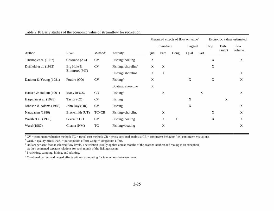
Economists have been estimating the value of recreation for over 40 years using methods such ascontingent valuation and the travel cost technique (U.S. Water Resources Council 1983). The firststudies that attempted to determine the relation of streamflow to riparian recreation value werepublished in the early 1980s (table 2.10). Such studies have focused on specific activities such asfishing or white water boating. Different studies measured different effects of flow on recreationvalue. For example, Bishop et al. (1987) estimated the immediate quality effect, and Johnson andAdams (1988) estimated the lagged quality effect. Only one study (Walsh et al. 1980) estimated acongestion effect. In some cases, effects that were not estimated were assumed nil. For example,Bishop et al. ignored a congestion effect for boating because use was fully controlled by permit,and Daubert and Young (1981) ignored congestion because they found no difference in WTPbetween the least and most crowded days. In other cases, effects were simply ignored because oflack of interest or data, or because of the limits of the valuation method employed.

2-25

Table 2.10 Early studies of the economic value of streamflow for recreation.

Measured effects of flow on valueb Economic values estimated

Immediate Lagged Trip Fishcaught

Flowvolumec

Author River Methoda Activity Qual. Part. Cong. Qual. Part.

Bishop et al. (1987) Colorado (AZ) CV Fishing; boating X X X

Duffield et al. (1992) Big Hole &Bitterroot (MT)

CV Fishing; shorelined X X X

Fishing+shoreline X X X

Daubert & Young (1981) Poudre (CO) CV Fishinge X X X X

Boating; shoreline X

Hansen & Hallam (1991) Many in U.S. CR Fishinge X X X

Harpman et al. (1993) Taylor (CO) CV Fishing X X

Johnson & Adams (1988) John Day (OR) CV Fishing X X

Narayanan (1986) Blacksmith (UT) TC+CB Fishing+shoreline X X X

Walsh et al. (1980) Seven in CO CV Fishing; boating X X X X

Ward (1987) Chama (NM) TC Fishing+boating X X

a CV = contingent valuation method; TC = travel cost method; CR = cross-sectional analysis; CB = contingent behavior (i.e., contingent visitation).b Qual. = quality effect; Part. = participation effect; Cong. = congestion effect.c Dollars per acre-foot at selected flow levels. The relation usually applies across months of the season; Daubert and Young is an exception as they estimated separate relations for each month of the fishing season.d Picnicking, camping, hiking, and relaxing.e Combined current and lagged effects without accounting for interactions between them.

2-26

Two studies (Daubert and Young 1981, Hansen and Hallam 1991) achieved a value estimate thatto some extent included both immediate and lagged effects. However, even in these casesinteractions between immediate and lagged effects, such as the effect of current fishing pressureon future fish populations and catch rates, were ignored.

Most of the studies in table 2.10 calculated a recreational value of instream flow, usually interms of acre-feet. Five of the studies estimated the change in marginal value of flow as flowchanged, but others only reported average values or marginal values for a common flow level.All else equal, unit value of flow is expected to be greater the: 1) more recreation activitiesoccur, 2) longer the stretch of river that receives recreation, 3) greater the number of tripsreceived per activity per mile of river, 4) better the quality of the recreation experience, and 5)less is the river flow level. Bishop et al. (1987) reported an average value of about 50¢/acre-ft forfishing and boating recreation downstream of Glen Canyon Dam in the relatively high-volumeColorado River. Hansen and Hallam (1991) reported a wide variety of current marginal valuesacross rivers, but values above $30/acre-ft were uncommon.

Shape of the Demand Curve for Instream Flow for Recreation

Daubert and Young (1981) and Duffield et al. (1992) presented demand functions that show themarginal value of instream flow dropping linearly with flow level from a maximum of $25 and$31/acre-ft, respectively, at 100 cfs, to minimums below zero at sufficiently high flows. Walsh etal. (1980) and Ward (1987) presented demand relations that show the marginal value of instreamflow rising to a maximum of $53 and $41/acre-ft, respectively, at moderate flow levels and thenfalling below zero at sufficiently high flows. Similarly, Narayanan’s (1986) demand functionrises to a maximum value of $1.32/acre-ft at moderate flows, and then drops to near zero at veryhigh flows. A rising marginal benefit curve at very low flows, as reported in the latter threestudies, indicates that flows must reach some minimum level before additions to flow have theexpected impact on the quality of recreation. The former two studies might also have found ademand curve that rises and then falls as flow increases if they had investigated very small flowlevels (below 100 cfs). In any case, once the minimum flow level is reached, the evidence fromthese five studies is that the demand curve is downward sloping.

Demand Monthly Distribution

All but one of the above studies gathered data for the principal recreation season—usually fromMay to October—and essentially assumed that the seasonal relation applied to each month withinthe season. Daubert and Young (1981) estimated separate relations of flow to value for eachseparate month during the season; however, the amount of data per individual month was small. Asa first approximation, the seasonal demand curve of aggregate WTP versus flow level could beapplied to each individual month of the recreation season, based on the assumption that variation inrecreation participation and quality across months is a function of changing flow level.

2-27

Nonuse Values

Nonmarket, or noncommodity, uses of water include not only recreation (discussed in theprevious section) but also preservation. Whereas riparian recreation involves an actual trip to ariver or stream, preservation of riparian areas and aquatic habitat does not. Nevertheless,preservation is valuable to many people, as evidenced by the millions of dollars annuallydonated to organizations such as the Nature Conservancy. Preservation is known by economistsas a nonuse value.

Using contingent valuation, economists have attempted to estimate preservation value, focusingon categories of nonuse value called existence and bequest values (see Brown 1993 for a surveyof nonuse value studies). A few of the nonuse value studies have focused on water flow. Forexample, Loomis (1987) studied the nonuse value of flows into Mono Lake, and Brown andDuffield (1995) studied the nonuse value of preserving flows in two Montana rivers. However,application of contingent valuation to estimate nonuse value remains controversial (Arrow et al.1993, Portney 1994). No doubt nonuse values for preserving certain species or ecosystems aresubstantial; however, there is no consensus that current methods accurately measure such values.In the absence of nonuse values for preservation of streamflows, preservation concerns can behandled in Aquarius using physical constraints.

Aggregate Consumptive Water Demand

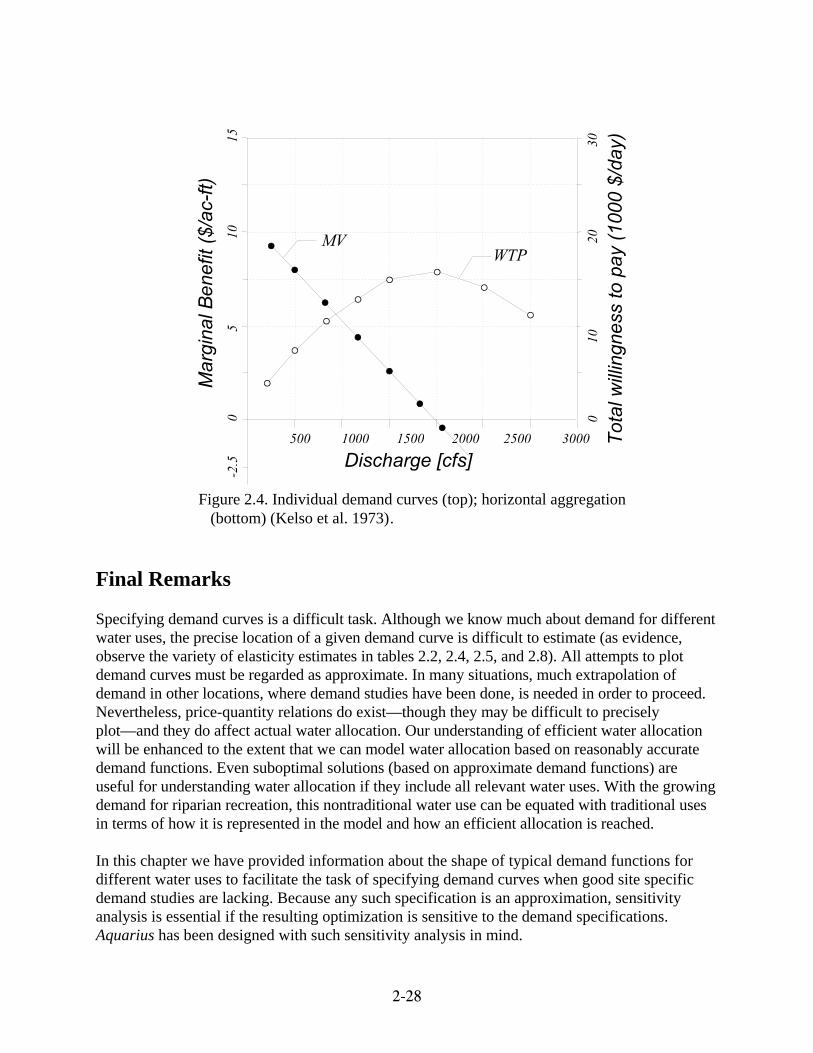
In reviewing various studies, we found that demands for different consumptive uses in Westernirrigation areas relate to each other roughly as depicted in the upper graph of figure 2.4. Thisfigure is from Kelso et al. (1973), who were conceptualizing water demand in Central Arizona.At one extreme, residential users are expected to demand relatively small quantities of water butbe willing to pay relatively high amounts. At the other extreme, agricultural users are expected todemand relatively large quantities of water but be willing to pay relatively low amounts.Commercial and industrial users are expected to fall in between these two extremes.

Aggregate consumptive water demand in an area competing for the same water supply can beexpressed as the horizontal sum of the individual demand curves, as in the lower graph of figure2.4. Although Aquarius allows agriculture and M&I to be represented by their individualdemand curves, the size of the water allocation problem may be reduced by combining these twocategories of use into an aggregate demand curve.

2-28

Figure 2.4. Individual demand curves (top); horizontal aggregation (bottom) (Kelso et al. 1973).

Final Remarks

Specifying demand curves is a difficult task. Although we know much about demand for differentwater uses, the precise location of a given demand curve is difficult to estimate (as evidence,observe the variety of elasticity estimates in tables 2.2, 2.4, 2.5, and 2.8). All attempts to plotdemand curves must be regarded as approximate. In many situations, much extrapolation ofdemand in other locations, where demand studies have been done, is needed in order to proceed.Nevertheless, price-quantity relations do exist—though they may be difficult to preciselyplot—and they do affect actual water allocation. Our understanding of efficient water allocationwill be enhanced to the extent that we can model water allocation based on reasonably accuratedemand functions. Even suboptimal solutions (based on approximate demand functions) areuseful for understanding water allocation if they include all relevant water uses. With the growingdemand for riparian recreation, this nontraditional water use can be equated with traditional usesin terms of how it is represented in the model and how an efficient allocation is reached.

In this chapter we have provided information about the shape of typical demand functions fordifferent water uses to facilitate the task of specifying demand curves when good site specificdemand studies are lacking. Because any such specification is an approximation, sensitivityanalysis is essential if the resulting optimization is sensitive to the demand specifications.Aquarius has been designed with such sensitivity analysis in mind.

3-1

Chapter 3Modeling of System Components

This chapter presents functional objectives, basic principles of operation, and modeling assumptionsfor the various water-using sectors included in the model. This material provides backgroundinformation for more detailed discussions in subsequent chapters about the development of benefitfunctions and the formulation of the general water allocation problem. The operationalcharacteristics of the system components presented here address only those elements that arerelevant for our modeling purposes. For detailed information concerning the management andoperation of water systems, consult specialized publications like those from the US Army Corps ofEngineers (1986).

The River Basin System

Water resource engineering has benefitted enormously from systems analysis, whichhas provided a framework for the conceptualization and analysis of river basinsystems. Hall and Dracup (1970) define a system as ". . . a set of elements which interact in a regular manner. Every system must have awell defined boundary or rule which specifies and distinguishes that which is in thesystem from the environment in which it exists. There will be inputs and outputs acrossthe boundary which must also be defined."

This general definition aptly characterizes a water resource system. The elements interacting withinthe system, such as reservoirs, irrigation demand areas, and instream recreation activities, are calledsystem components. System boundaries are defined by the flow network, which the analyst createsto represent the river basin to be modeled. The network specifies which components will be part ofthe system. Inputs, which consist of information necessary to simulate the operation of a systeminclude, among many others, natural flows, water demands for irrigation, instream flowrequirements, and the price of energy. As explained latter, some of the inputs can be controlled bythe analyst, but others are portrayed as uncontrollable inputs. Outputs are quantitative measures ofthe system performance that consist of many component objectives. Depending on the objectives,performance may be measured in terms of monetary values, amount of energy produced, biologicalindexes, or amount of water supplied to offstream demand areas.

Aquarius is a modeling system that helps create a conceptualization, and usually a simplification,of a real-world system. The degree of detail with which each component is characterized varies withthe desired accuracy. For a model to reflect the real behavior of a system with accuracy, it mustpreserve all the essential operational characteristics of the river basin. For a generalized model, suchas the one proposed here, this is a challenge.

3-2

Water Sources

Two water sources are typically found in a river basin: surface andsubsurface water. Both can be represented by Aquarius. Although theyare parts of the same resource, differences in their availability, cost andadministration often cause them to be treated separately. For many yearshydrogeologists and engineers have been developing water supplysources for a vast array of purposes. As the demand of water increased,

new water sources had to be developed. Only during the last few years, and as a result of a largerenvironmental awareness and an increase in the cost of providing additional water, there has beena change in paradigm, where the development of new water sources has been subordinated to priorconservation efforts and more efficient use of the water already available.

Surface water, water which remains on top of the land, refers to the natural flows conducted by thedrainage network of a basin, as measured by a gaging station at a given location of a water course.Flow records can extend from just a few years to 100 years or more. At least ten years are neededto have an approximate idea of the water yield of the catchment. Records longer than 50 years areneeded to begin to explain in detail the temporal variability of the flow time series at the site. Asurface-water-source (SWS) in general can be either controlled or uncontrolled flows (regulated orunregulated), although for our purpose a SWS is always interpreted as uncontrolled (unregulated)flows.

Subsurface water supplies are contained in the saturated portion of the soil or rock profile. Anunderground reservoir is usually part of a regional aquifer that may expand much farther than theboundaries of the catchment of interest. A ground-water-source (GWS) is normally developed fromwells or springs which are usually located near the demand area. Because ground water has to bepumped from below the surface, it constitutes a controlled water supply.

Where surface and ground water are hydraulically connected, the use of ground water can altersurface flows, and vice versa. This interrelationship may generate adverse effects on downstreamthird parties. Considering the conjunctive use of surface and ground water would add a newdimension to the water supply component. Aquarius does not model the hydrologic interactionbetween the two water sources, although it can simulate the pumping of ground water (GWP) to thesurface.

Rising population and incomes have led to increasing demands for water in agriculture, industry andother uses, and thus to increasing pressures on water supplies. Legal, institutional and economicconstraints will largely determine whether surface or ground water supplies are first to be exploited.In many locations the cost of ground water is higher than the cost of surface water due to pumpingcosts. But where surface water is scarce, the cost of ground water may be less than it is for surfacewater, making augmentation of the supply using ground water sources a viable economic alternative.However, where the pumping rate exceeds recharge, water tables drop and pumping costs graduallyincrease, perhaps shifting the pressure back to surface water supplies.

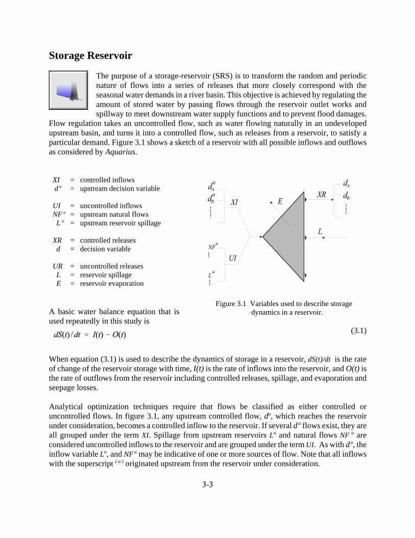
3-3

Figure 3.1 Variables used to describe storage dynamics in a reservoir.

Storage Reservoir

The purpose of a storage-reservoir (SRS) is to transform the random and periodicnature of flows into a series of releases that more closely correspond with theseasonal water demands in a river basin. This objective is achieved by regulating theamount of stored water by passing flows through the reservoir outlet works andspillway to meet downstream water supply functions and to prevent flood damages.

Flow regulation takes an uncontrolled flow, such as water flowing naturally in an undevelopedupstream basin, and turns it into a controlled flow, such as releases from a reservoir, to satisfy aparticular demand. Figure 3.1 shows a sketch of a reservoir with all possible inflows and outflowsas considered by Aquarius.

XI = controlled inflows d u = upstream decision variable

UI = uncontrolled inflows NF u = upstream natural flows L u = upstream reservoir spillage

XR = controlled releases d = decision variable

UR = uncontrolled releases L = reservoir spillage E = reservoir evaporation

A basic water balance equation that isused repeatedly in this study is

(3.1)

When equation (3.1) is used to describe the dynamics of storage in a reservoir, dS(t)/dt is the rateof change of the reservoir storage with time, I(t) is the rate of inflows into the reservoir, and O(t) isthe rate of outflows from the reservoir including controlled releases, spillage, and evaporation andseepage losses.

Analytical optimization techniques require that flows be classified as either controlled oruncontrolled flows. In figure 3.1, any upstream controlled flow, du, which reaches the reservoirunder consideration, becomes a controlled inflow to the reservoir. If several d u flows exist, they areall grouped under the term XI. Spillage from upstream reservoirs Lu and natural flows NF u areconsidered uncontrolled inflows to the reservoir and are grouped under the term UI. As with d u, theinflow variable Lu, and NF u may be indicative of one or more sources of flow. Note that all inflowswith the superscript ( u ) originated upstream from the reservoir under consideration.

3-4

Among reservoir outflows, we present two groups: the controlled releases d and the uncontrolledreservoir releases, such as spills L and evaporation losses E, grouped under the term UR (not depictedin figure 3.1). As more than one controlled release d is possible, we group them under the term XR.Controlled releases encompass water for offstream uses such as hydropower, municipal water supplyand irrigation demand areas. Controlled releases for instream uses include flood control in flood-prone river reaches, water-based recreation in rivers and lakes and reservoir releases to protect theintegrity of a river ecosystem.

Using the notation indicated above and substituting the time index i for t to indicate discrete timeintervals, the inflow to a reservoir during any time period i is expressed as a function of

(3.2)

where the expression is used to indicate the contribution of upstream controlvariables to the reservoir inflows. Similarly, total outflows from the reservoir are expressed by

(3.3)

where again the expression groups all controlled reservoir releases andencompasses spills and evaporation losses.

The physical characteristics of a reservoir are defined by two basic functions: the elevation-storagecurve, which defines the variation of the storage capacity in the reservoir with the water surfaceelevation; and the area-storage curve, which represents the area enclosed by the reservoir at differentelevations. Both functional relations can often be approximated by the following power functions

(3.4a)

(3.4b)

where S is storage volume in millions-of-cubic-meters (Mcm), A is reservoir area in squarekilometers (Km2 ), H is the depth of water above a given datum in meters (m), and c and d are theparameters of the analytical models. Because of natural changes, such as sedimentation, occurringin the reservoir over time, the parameters may need to be recomputed after some years of operation.Other functional forms, such as a polynomial, can be used instead of (3.4a,b) if a good fit cannot beobtained with the power functions.

In addition to spills, two types of water losses to consider in a reservoir are evaporation and seepage.Both are functions of the level of storage in the reservoir. Evaporation is estimated by multiplyingthe surface area of the lake, computed using (3.4b), times the seasonal evaporation rate inmillimeters.

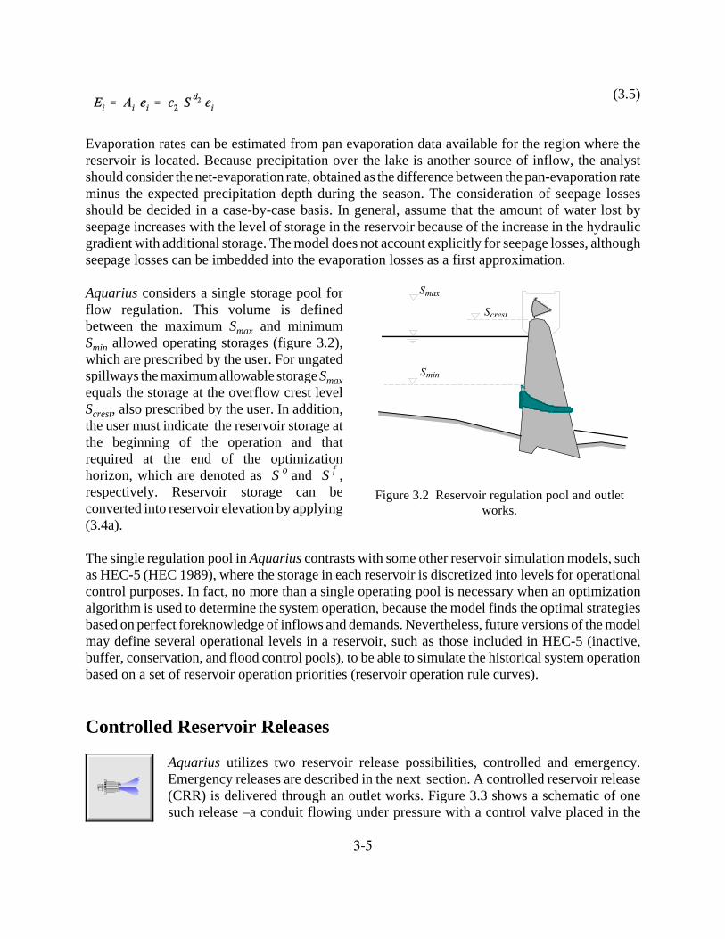
3-5

Figure 3.2 Reservoir regulation pool and outletworks.

(3.5)

Evaporation rates can be estimated from pan evaporation data available for the region where thereservoir is located. Because precipitation over the lake is another source of inflow, the analystshould consider the net-evaporation rate, obtained as the difference between the pan-evaporation rateminus the expected precipitation depth during the season. The consideration of seepage lossesshould be decided in a case-by-case basis. In general, assume that the amount of water lost byseepage increases with the level of storage in the reservoir because of the increase in the hydraulicgradient with additional storage. The model does not account explicitly for seepage losses, althoughseepage losses can be imbedded into the evaporation losses as a first approximation.

Aquarius considers a single storage pool forflow regulation. This volume is definedbetween the maximum Smax and minimumSmin allowed operating storages (figure 3.2),which are prescribed by the user. For ungatedspillways the maximum allowable storage Smaxequals the storage at the overflow crest levelScrest, also prescribed by the user. In addition,the user must indicate the reservoir storage atthe beginning of the operation and thatrequired at the end of the optimizationhorizon, which are denoted as S o

and S f ,respectively. Reservoir storage can beconverted into reservoir elevation by applying(3.4a).

The single regulation pool in Aquarius contrasts with some other reservoir simulation models, suchas HEC-5 (HEC 1989), where the storage in each reservoir is discretized into levels for operationalcontrol purposes. In fact, no more than a single operating pool is necessary when an optimizationalgorithm is used to determine the system operation, because the model finds the optimal strategiesbased on perfect foreknowledge of inflows and demands. Nevertheless, future versions of the modelmay define several operational levels in a reservoir, such as those included in HEC-5 (inactive,buffer, conservation, and flood control pools), to be able to simulate the historical system operationbased on a set of reservoir operation priorities (reservoir operation rule curves).

Controlled Reservoir Releases

Aquarius utilizes two reservoir release possibilities, controlled and emergency.Emergency releases are described in the next section. A controlled reservoir release(CRR) is delivered through an outlet works. Figure 3.3 shows a schematic of onesuch release –a conduit flowing under pressure with a control valve placed in the

3-6

Figure 3.3 Section of an outlet pipe with downstream valve control

downstream end of the conduit (one of manypossible arrangements).

In Aquarius a reservoir allows controlled flowreleases through up to three outlet works(depicted in figure 3.1 by small trianglesattached to the dam wall): C one on each side of the dam wall, for

offstream releases;C a third discharge at the center, for

instream releases.

The center outlet may povide water fordownstream water demands, and also may actas an emergency waterway during extremelyrich water periods as described below .

In Aquarius water demands that are “directly” linked to a reservoir (i.e., there is a single linkconnecting the reservoir to the demand) put a water call on the stored water. On the other hand,water demands that are not directly linked to a reservoir providing water to the demand (i.e., thereis more than one link between the reservoir and the demand, so they are “indirectly” linked) do notautomatically allow a call on the stored water. To allow for a call in this case the user mustimplement a special model component called an indirect-water-call (IWC). This dummy componentenables the mathematical connection between the reservoir and the indirectly-linked demand. Thedemonstration networks in Figure 6.3 and Chapter 8 provide examples of the capabilities of thissingular element.

Aquarius computes the outflowing discharge Qvalve of a reservoir using the hydraulic equation forflow in a closed pipe system

(3.6)

where A is the area of the conduit, KL is the loss coefficient for the whole discharge system, and HTis the total head needed to overcome the various head losses to produce discharge. For details on thehydraulic calculation of (3.6), in particular the term KL, see USBR (1977).

Emergency Reservoir Releases

Excess water that cannot be released from the reservoir for some beneficial use alsofinds its way out of the reservoir through emergency structures, named here asemergency-reservoir-release (ERR) (and depicted by the schematics of Figure 3.2).

3-7

Figure 3.4 Section of a gate-controlled spillway.

Aquarius supports two types of spillages(with the limitations indicated below):C an open channel spillway;C an outlet works conduit flowing under

pressure (central reservoir outlet)

Spillway crest gates are used to control thespillway discharge according to pre-established operation rules; ungated spillwaysare not subject to any control. For gate-controlled spillways with partial gate opening(figure 3.4), outflow releases occur as orificeflow. The controlled discharge Qspill iscomputed by (3.7a), where l is the net lengthof the spillway, H1 indicates the total head onthe upper edge of the gate, H2 is the total headon the lower edge (both refer to the level of zero outflow), and C denotes the coefficient of dischargeof the overfall spillway, a function of the gate opening and crest arrangement as indicated by (3.7b)

(3.7a)

(3.7b)

The capacity of the spillway to pass a flood wave during a given time interval depends on the watersurface elevation in the reservoir forebay at the beginning of the interval and on the length of thesimulation time step. Iterative computational procedures are needed to estimate the gate-controlledspillway discharge coefficient C and to compute the residual reservoir storage volume at the end ofthe simulation time step. However, detailed simulation of the spillway operation becomes relevantonly for small-time simulation steps (hourly, daily). For monthly time steps, and even weekly attimes depending on the size of the reservoir and inflow conditions, detailed operation of the spillwayis usually omitted. For monthly time steps it is convenient to pass any excess flood waterdownstream of the reservoir as a block, without attempting any spillway operation procedure.Aquarius computes the total outflowing discharge Qspill of a reservoir through an ungated spillwayby means of the following power function

(3.8)

where the only new variable is He, the total head on the crest. Knowing the water surface elevationin the reservoir (obtained from the elevation-storage function) and the elevation of the spillway crestHcrest (level of zero outflow), the model computes He and the volume spilled during the time intervalof analysis. This volume is checked against the maximum discharge capacity of the spillway to avoidthe overtopping of the dam. The user should prescribe the basic information indicated in (3.8).

3-8

As indicated in the previous subsection, the central outlet of a reservoir may play the dual functionof releasing water to satisfy downstream demands and at the same time releasing excess waterduring extremely rich water periods (the reservoir water surface can be at any level above theminimum operational level Smin). Thus, the central reservoir outlet becomes a mandatory downstreamconnection for all reservoirs. The outflow equation is given by (3.6).

In addition to the capability of the reservoir to release excess water through the emergency structuresintroduced above, Aquarius includes a conceptual system component, termed the spill-controller(SPC), which helps minimize reservoir spillages. The spill controller acts upon the reservoir towhich it is connected to discourage spillages, and indirectly, over all the system componentsupstream that provide inflows to the reservoir under consideration (more details about thecharacteristics of this component are given in Chapter 5). The spill controller does not perform adetailed simulation of the spillway operation. In fact, operation of a gate-controlled spillway isunnecessary for monthly time steps of simulation, as in this model (the model passes any excessflood water downstream of the reservoir as a block).

Hydropower Generation

Operation of an electric power system involves considering three basic componentsor subsystems, the: i) energy sources (thermal, hydro, nuclear); ii) electric networkcomponents (generators, transformers, transmission lines); and iii) energy demandor load, constituted by a large number of electrical devices connected by thecustomers to the system. Each one of these components is a highly specialized

engineering field that may require detailed modeling efforts depending upon the problem underconsideration (e.g., El-Hawary and Christensen 1979). Aquarius deals only with the energy sourcecomponent of hydropower (HPW).

In hydropower systems, hydraulic turbines convert the energy in water stored in reservoirs or otherstructures into kinetic energy, which in turn is converted into electric energy by the generators.Hydropower facilities are typically hydraulically linked to reservoirs, and it is convenient to modelthe power plant and the reservoir as a unit. Aquarius can represent the following types ofhydropower installations:

C storage plants, with considerable storage capacity in the reservoir that feeds the powerplant;C run-of-river plants, with negligible storage capacity and use water as it becomes available.

A hydropower installation is treated as a variable-head powerplant when the net hydraulic headacting on the turbines changes with water surface elevation changes in the reservoir. Typical layoutsof variable-head plants show the powerhouse as: an integral part of the dam; a separate unitconstructed at the toe of the dam (figure 3.5, left); or built at a distance from the dam and connectedto the reservoir by tunnel and penstock. A fixed-head powerplant operates under a nearly constantnet hydraulic head and is connected to the reservoir by a canal or some other type of open-channelstructure (figure 3.5, right). This is also called a canal powerplant.

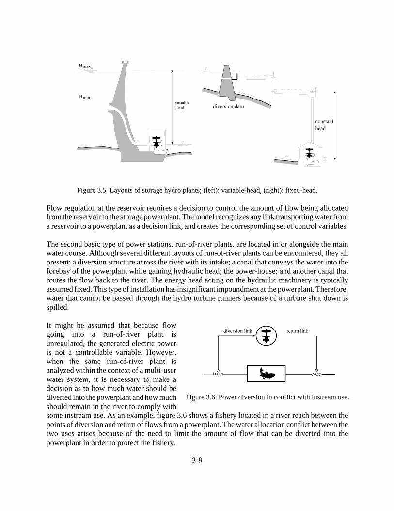
3-9

Figure 3.6 Power diversion in conflict with instream use.

Figure 3.5 Layouts of storage hydro plants; (left): variable-head, (right): fixed-head.

Flow regulation at the reservoir requires a decision to control the amount of flow being allocatedfrom the reservoir to the storage powerplant. The model recognizes any link transporting water froma reservoir to a powerplant as a decision link, and creates the corresponding set of control variables.

The second basic type of power stations, run-of-river plants, are located in or alongside the mainwater course. Although several different layouts of run-of-river plants can be encountered, they allpresent: a diversion structure across the river with its intake; a canal that conveys the water into theforebay of the powerplant while gaining hydraulic head; the power-house; and another canal thatroutes the flow back to the river. The energy head acting on the hydraulic machinery is typicallyassumed fixed. This type of installation has insignificant impoundment at the powerplant. Therefore,water that cannot be passed through the hydro turbine runners because of a turbine shut down isspilled.

It might be assumed that because flowgoing into a run-of-river plant isunregulated, the generated electric poweris not a controllable variable. However,when the same run-of-river plant isanalyzed within the context of a multi-userwater system, it is necessary to make adecision as to how much water should bediverted into the powerplant and how muchshould remain in the river to comply withsome instream use. As an example, figure 3.6 shows a fishery located in a river reach between thepoints of diversion and return of flows from a powerplant. The water allocation conflict between thetwo uses arises because of the need to limit the amount of flow that can be diverted into thepowerplant in order to protect the fishery.

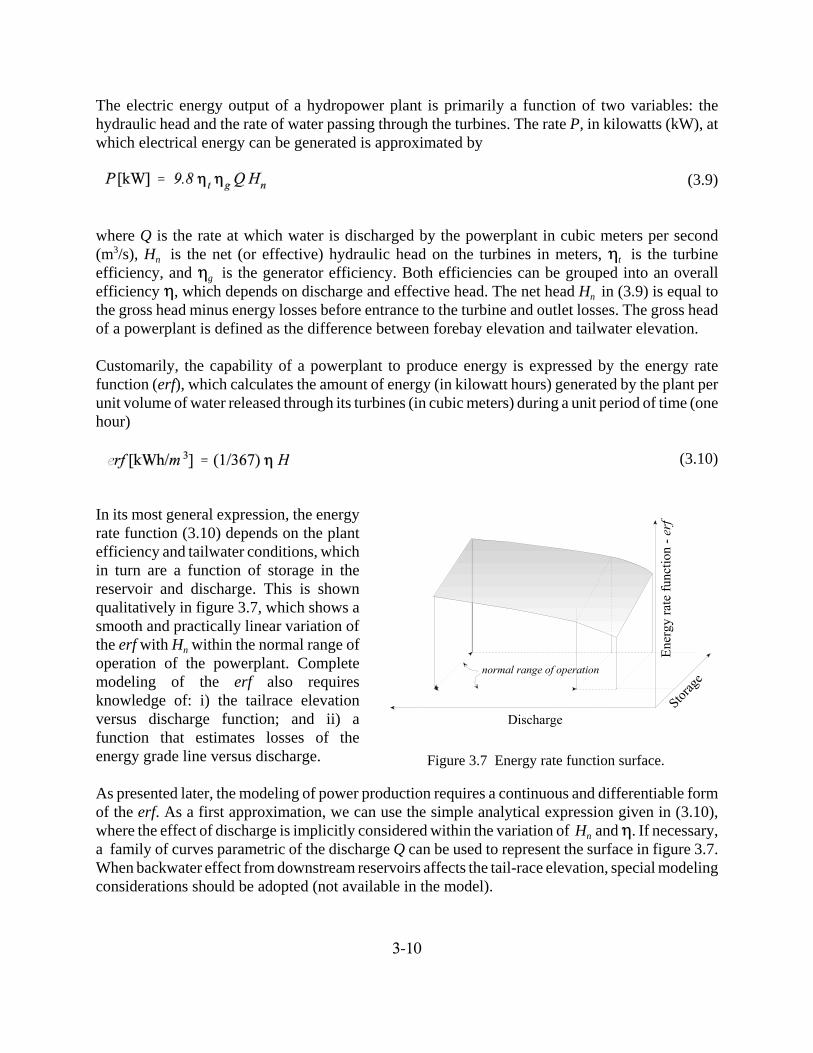
3-10

Figure 3.7 Energy rate function surface.

The electric energy output of a hydropower plant is primarily a function of two variables: thehydraulic head and the rate of water passing through the turbines. The rate P, in kilowatts (kW), atwhich electrical energy can be generated is approximated by

(3.9)

where Q is the rate at which water is discharged by the powerplant in cubic meters per second(m3/s), Hn is the net (or effective) hydraulic head on the turbines in meters, 0t is the turbineefficiency, and 0g is the generator efficiency. Both efficiencies can be grouped into an overallefficiency 0, which depends on discharge and effective head. The net head Hn in (3.9) is equal tothe gross head minus energy losses before entrance to the turbine and outlet losses. The gross headof a powerplant is defined as the difference between forebay elevation and tailwater elevation.

Customarily, the capability of a powerplant to produce energy is expressed by the energy ratefunction (erf), which calculates the amount of energy (in kilowatt hours) generated by the plant perunit volume of water released through its turbines (in cubic meters) during a unit period of time (onehour)

(3.10)

In its most general expression, the energyrate function (3.10) depends on the plantefficiency and tailwater conditions, whichin turn are a function of storage in thereservoir and discharge. This is shownqualitatively in figure 3.7, which shows asmooth and practically linear variation ofthe erf with Hn within the normal range ofoperation of the powerplant. Completemodeling of the erf also requiresknowledge of: i) the tailrace elevationversus discharge function; and ii) afunction that estimates losses of theenergy grade line versus discharge.

As presented later, the modeling of power production requires a continuous and differentiable formof the erf. As a first approximation, we can use the simple analytical expression given in (3.10),where the effect of discharge is implicitly considered within the variation of Hn and 0. If necessary,a family of curves parametric of the discharge Q can be used to represent the surface in figure 3.7.When backwater effect from downstream reservoirs affects the tail-race elevation, special modelingconsiderations should be adopted (not available in the model).

3-11

Agriculture Irrigation

The lack of precipitation in many arid and semi-arid regions precludes cropproduction unless moisture is supplemented with irrigation (IRR) water. Historically,the need to reduce these moisture deficiencies has led to development of agriculturalwater supply projects, which are the largest consumptive users of water in a riverbasin. In the Western United States, such projects store runoff that occurs during the

spring snow melt and releases it during the drier period of the growing season.

Large irrigation developments are composed of a complex array of water related structures for flowregulation, diversion, conveyance, distribution, and application. Once the irrigation water is appliedto a field, additional structures may be required for capturing and transporting return flows back tothe main water course. Aquarius deals with the first and last stages of the agricultural water usesystem: i) the supply of water to the demand area, and ii) the physical link to return the non-consumptive portion of that supply to the system. The model does not analyze the intricacies of thedistribution and application subsystems.

Water for irrigation may be diverted directly (i.e., without prior storage) from a river to a farm ifnatural streamflow is sufficient. However, low flows in a river may severely limit the capacity ofa natural system to reliably supply water, particularly for large irrigation developments. By creatinga storage capacity between the water source and the demand area, the reliability of the water sourceincreases dramatically. The net increase in dependable water supply, the firm yield, is a directfunction of reservoir storage. Typically, a storage capacity that supplies irrigation water holds aportion of the incoming water in storage during the high flow season until the natural flow recedesto the point where it is no longer sufficient to meet the downstream irrigation demand. Releases ofstored water from the reservoir are then used to augment flows in the river to meet the demand.Often the need for augmented flows persists until the end of the growing season. Even during thewinter months, small amounts of water may still be allocated to the demand area for domestic use,stock water, or other purposes.

In addition to surface water, ground water can be used to satisfy the demand of the agriculturalsector. When the marginal cost of acquiring surface water for satisfying irrigation demand increases,ground water may become an economical alternative. In summary, Aquarius can simulate thefollowing possible schemes for providing water supply to an agriculture demand area: C direct water diversion from existing flows in the river to an irrigation area;C water released from a storage reservoir into a river and then withdrawn at a downstream

diversion point; C water released from a storage reservoir into a canal or conduit, rather than into the riverbed, and

conveyed directly to the demand area;C ground water pumping to an irrigation area.

Whether irrigation water is pumped from an aquifer, diverted directly from a reservoir, or from ariver channel (using a diversion dam), the model individualizes the decision links in the network that

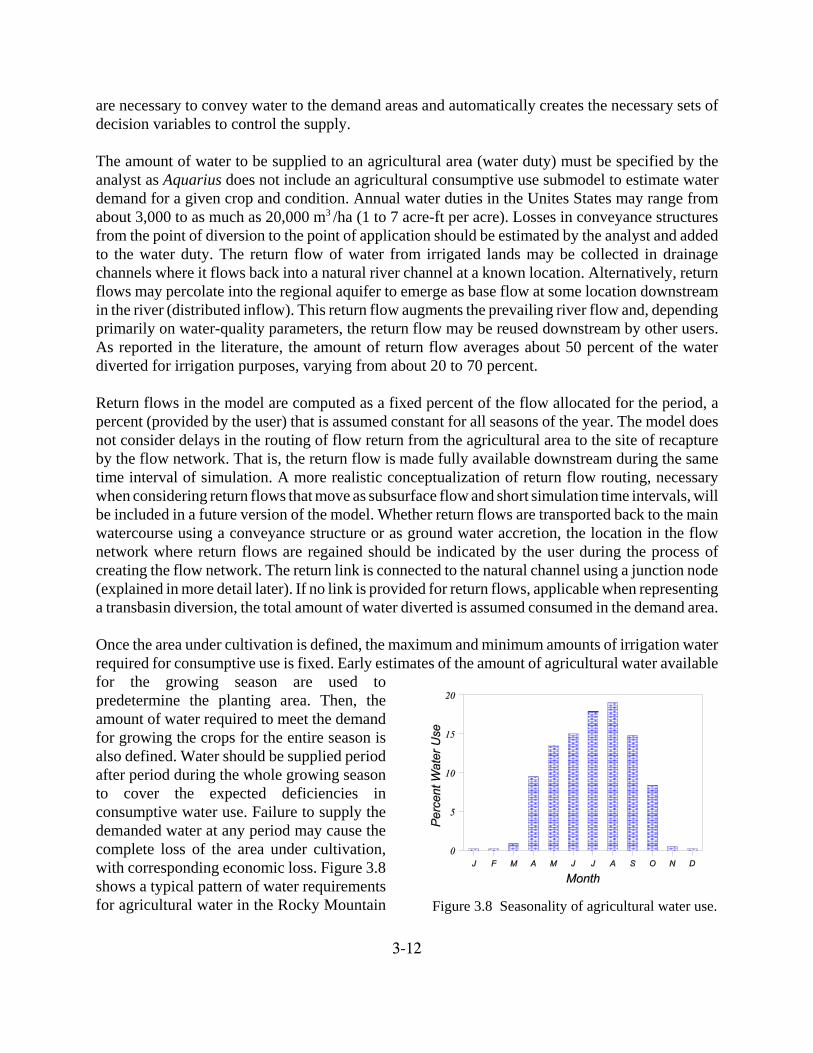
3-12

Figure 3.8 Seasonality of agricultural water use.

are necessary to convey water to the demand areas and automatically creates the necessary sets ofdecision variables to control the supply.

The amount of water to be supplied to an agricultural area (water duty) must be specified by theanalyst as Aquarius does not include an agricultural consumptive use submodel to estimate waterdemand for a given crop and condition. Annual water duties in the Unites States may range fromabout 3,000 to as much as 20,000 m3 /ha (1 to 7 acre-ft per acre). Losses in conveyance structuresfrom the point of diversion to the point of application should be estimated by the analyst and addedto the water duty. The return flow of water from irrigated lands may be collected in drainagechannels where it flows back into a natural river channel at a known location. Alternatively, returnflows may percolate into the regional aquifer to emerge as base flow at some location downstreamin the river (distributed inflow). This return flow augments the prevailing river flow and, dependingprimarily on water-quality parameters, the return flow may be reused downstream by other users.As reported in the literature, the amount of return flow averages about 50 percent of the waterdiverted for irrigation purposes, varying from about 20 to 70 percent.

Return flows in the model are computed as a fixed percent of the flow allocated for the period, apercent (provided by the user) that is assumed constant for all seasons of the year. The model doesnot consider delays in the routing of flow return from the agricultural area to the site of recaptureby the flow network. That is, the return flow is made fully available downstream during the sametime interval of simulation. A more realistic conceptualization of return flow routing, necessarywhen considering return flows that move as subsurface flow and short simulation time intervals, willbe included in a future version of the model. Whether return flows are transported back to the mainwatercourse using a conveyance structure or as ground water accretion, the location in the flownetwork where return flows are regained should be indicated by the user during the process ofcreating the flow network. The return link is connected to the natural channel using a junction node(explained in more detail later). If no link is provided for return flows, applicable when representinga transbasin diversion, the total amount of water diverted is assumed consumed in the demand area.

Once the area under cultivation is defined, the maximum and minimum amounts of irrigation waterrequired for consumptive use is fixed. Early estimates of the amount of agricultural water availablefor the growing season are used topredetermine the planting area. Then, theamount of water required to meet the demandfor growing the crops for the entire season isalso defined. Water should be supplied periodafter period during the whole growing seasonto cover the expected deficiencies inconsumptive water use. Failure to supply thedemanded water at any period may cause thecomplete loss of the area under cultivation,with corresponding economic loss. Figure 3.8shows a typical pattern of water requirementsfor agricultural water in the Rocky Mountain

3-13

Figure 3.9 Seasonality of municipal and industrial use.

region of the Western U.S., with the maximum demand occurring at the end of the summer. Incontrast to the well defined growing season shown in figure 3.8, other agricultural areas have a year-round growing season. Aquarius allows the user to prescribe the total amount of water to bedelivered to an irrigation area during the entire growing season, the seasonal pattern of thedeliveries, and even the maximum and minimum volumes at each time interval.

Municipal and Industrial Water Supply

Historically, urban water has been supplied separately from other uses, althoughmunicipal water supply intakes are sometimes provided in dams built for otherpurposes. For example, in some locations municipal water is conducted incombination with agricultural water where both use the same installations. Amunicipality water demand can be modeled as a single user using the system

component described here, or it can be integrated with some other demand, using a combineddemand curve. In this section, we concentrate on the basic operational characteristics and modelingof water supply for household, industrial, commercial, public and other activities, usually termedmunicipal-and-industrial (M&I). The model simulates the water demand in the M&I zone as a singleblock, transporting the allocated water from the flow regulation subsystem to the boundary of theM&I area. The model makes no consideration of the distribution subsystem inside the demand area.

Practically all river systems supply water for municipal and industrial use. Supply of M&I water ina highly reliable manner is usually given a high priority. As a whole, M&I water demand isrelatively small compared with irrigation demand. The normal range of demand from an urban areais from 150 to 400 lpcd (liters per capita per day) (40 to 100 gallons per capita per day), althoughthis varies considerably with the climate and economic conditions of the demand area. In arid andsemi-arid regions with an abundant and low-cost water supply, the average annual demand can beup to twice those values. The amount of water supplied for municipal and industrial uses is fairlyuniform through the year, except in areas with substantial lawn sprinkling. Although indoor useremains practically constant over the year, the sprinkling of open areas contributes to the seasonalityof urban demand.

Figure 3.9 shows the typical monthlydistribution of water use for a city in a semi-arid region in the U.S. The almost uniformdistribution in figure 3.9 contrasts with thehighly seasonal demand in figure 3.8 forirrigation.

Similar to irrigation water, M&I water maybe withdrawn directly from the undergroundaquifer, from the stream using open channelflow diversions or from reservoirs thatrelease water from storage into canals or

3-14

pipes. The four schemes of water supply listed previously for agricultural water can also besimulated for M&I use by Aquarius. Whether M&I water is diverted from reservoirs, diversion damsor directly from a river or aquifer, the model detects decision links in the network that convey waterinto M&I demand areas and automatically creates the necessary sets of decision variables to controlthe supply.

Return flows from urban areas are collected by a network of sewers and transported to treatmentplants before being finally restored to the river channel. It is generally reported that between 60 and90 percent of the total water supplied to an M&I area is returned as waste water, with small changesin water quality after treatment. The return flow augments the prevailing river flow and, dependingon water-quality parameters, it may be reused downstream by some other water users. Return flowsin the model are computed as a percent (entered by the user) of the total allocated inflow; thispercentage is held constant for all seasons of the year.

Losses in conveyance structures from the point of diversion to the point of use should be estimatedby the analyst and added to the water demand. As indicated earlier for irrigation return flows, thepresent version of the model cannot delay flows returning from the demand area to some later timestep, although for M&I use this is less critical. While building the flow network, the user shouldindicate the junction site where M&I return flows are routed back to the main watercourse (usinga left- or right-bank junction node). If no link for return flows is provided, the model assumes thatthe total amount of diverted water is consumed in the demand area.

Instream Water Recreation

The importance of instream-water-recreation (IWR) activities such as fishing,boating, swimming, and picnicking at the water's edge, has recently increaseddramatically. Throughout earlier decades, when many of the reservoirs anddiversion works in the US were constructed, recreation was an incidental use ofrivers, streams, lakes and reservoirs. After passage of the Flood Control Act of

1936, which required benefit-cost analysis of federal water development projects, recreation wasoften given formal recognition. Although the expected recreation at a new reservoir was countedas a benefit, the reduction in recreation quantity or quality in a dewatered channel downstreamwas ignored.

As water development continued to alter instream recreational opportunities and as incomes andleisure time grew, stream-based recreation received enhanced recognition. The federalgovernment began to require more formal consideration of recreation in analyses of waterdevelopments. Consider the procedures for evaluation of water and related land resourcespromulgated by the Water Resources Council during the 1960s and 1970s, passage of theNational Environmental Policy Act of 1969, the 1965 and 1972 amendments to the Clean WaterAct requiring states to specify designated uses of their water bodies, and the 1986 amendmentsto the Federal Water Power Act requiring that the Federal Energy Regulatory Commission giveequal consideration to conservation in the licensing of hydroelectric projects. Thus, reservoir

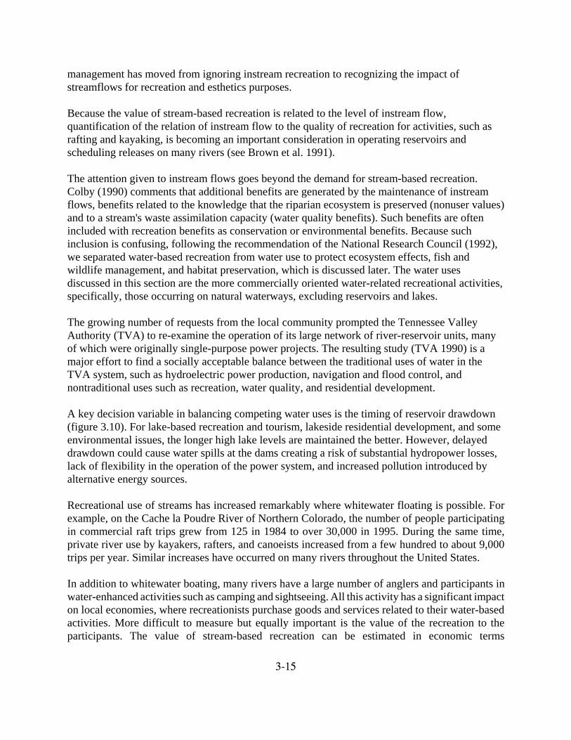
3-15

management has moved from ignoring instream recreation to recognizing the impact ofstreamflows for recreation and esthetics purposes.

Because the value of stream-based recreation is related to the level of instream flow,quantification of the relation of instream flow to the quality of recreation for activities, such asrafting and kayaking, is becoming an important consideration in operating reservoirs andscheduling releases on many rivers (see Brown et al. 1991).

The attention given to instream flows goes beyond the demand for stream-based recreation.Colby (1990) comments that additional benefits are generated by the maintenance of instreamflows, benefits related to the knowledge that the riparian ecosystem is preserved (nonuser values)and to a stream's waste assimilation capacity (water quality benefits). Such benefits are oftenincluded with recreation benefits as conservation or environmental benefits. Because suchinclusion is confusing, following the recommendation of the National Research Council (1992),we separated water-based recreation from water use to protect ecosystem effects, fish andwildlife management, and habitat preservation, which is discussed later. The water usesdiscussed in this section are the more commercially oriented water-related recreational activities,specifically, those occurring on natural waterways, excluding reservoirs and lakes.

The growing number of requests from the local community prompted the Tennessee ValleyAuthority (TVA) to re-examine the operation of its large network of river-reservoir units, manyof which were originally single-purpose power projects. The resulting study (TVA 1990) is amajor effort to find a socially acceptable balance between the traditional uses of water in theTVA system, such as hydroelectric power production, navigation and flood control, andnontraditional uses such as recreation, water quality, and residential development.

A key decision variable in balancing competing water uses is the timing of reservoir drawdown(figure 3.10). For lake-based recreation and tourism, lakeside residential development, and someenvironmental issues, the longer high lake levels are maintained the better. However, delayeddrawdown could cause water spills at the dams creating a risk of substantial hydropower losses,lack of flexibility in the operation of the power system, and increased pollution introduced byalternative energy sources.

Recreational use of streams has increased remarkably where whitewater floating is possible. Forexample, on the Cache la Poudre River of Northern Colorado, the number of people participatingin commercial raft trips grew from 125 in 1984 to over 30,000 in 1995. During the same time,private river use by kayakers, rafters, and canoeists increased from a few hundred to about 9,000trips per year. Similar increases have occurred on many rivers throughout the United States.

In addition to whitewater boating, many rivers have a large number of anglers and participants inwater-enhanced activities such as camping and sightseeing. All this activity has a significant impacton local economies, where recreationists purchase goods and services related to their water-basedactivities. More difficult to measure but equally important is the value of the recreation to theparticipants. The value of stream-based recreation can be estimated in economic terms

3-16

Figure 3.10 Forces acting on lake drawdown (TVA 1990).

commensurate with the values of more traditional water uses by allowing such values to beincorporated into the multipurpose modeling process. Because stream-based recreation is not soldin competitive markets like many other water projects, the recreation value estimation requiresspecialized approaches. Nevertheless, this should not discourage attention to instream economicbenefits. Recent studies (e.g., Duffield et al. 1992) have provided strong evidence that instreambenefits can sometimes exceed those generated by offstream uses, and that gains are achievable onsome systems by reallocating water from consumptive to instream uses. Similarly, Colby (1990)argues that instream values are high enough to compete in the market for water rights with offstreamuses when important recreation sites and wildlife species are involved.

Water recreation has marked seasonal characteristics, similar to agricultural water use. The numberof visitors can vary from very low during cold winter months to the very high during the spring andsummer. For recreation, seasonality is also at the daily level as weekday use is typically much lowerthan weekends use. This suggests the need to use very short-time intervals when simulating theoperation of a river system that includes recreation activities (Morel-Seytoux et al. 1995).

The use of water for instream recreation is not exempt from conflicts with other uses. For instance,maintaining higher instream flows during the weekends increases opportunities for activities suchas kayaking and boating but conflicts with electric power objectives because electricity demandtends to be lower during the weekends. Extra weekend releases may reduce the capability of thepowerplants to meet energy and power demand during weekdays because of lower reservoir levels.Helping solve conflicts of this nature is the focus of multipurpose water system analysis.

3-17

Reservoir with Lake Recreation

In addition to the instream recreation activities described previously, other water-related recreational activities are practiced by the general public on and aroundreservoirs and lakes. Residential development is also a common shoreline use wherethe land is privately owned. Reservoir-with-lake-recreation (RLR) activities includefishing, boating including water skiing, swimming, camping, picnicking and

sightseeing. These activities have become an important use of some reservoirs. Indeed, it is nolonger uncommon for systems to be operated to maximize reservoir recreation activities during thesummer months at the expense of other water uses such as hydropower.

Reservoir recreation is typically a highly seasonal activity, similar to instream recreation water use.The number of visitors is higher during the summer months, particularly for water sports activitiessuch as sailing and water skiing. The same requirement for short-time intervals of analysis discussedfor instream recreation applies here.

The use of water for reservoir recreation is not exempt from conflicts with other uses. Reservoiroperation for recreation tends to keep the water surface high and minimize water level fluctuation.Excessive drawdown and large fluctuations may prevent sailing, disturbs access to docks and createsunpleasant view for visitors, campers and home owners living along the reservoir shoreline.Examples of such conditions include a water supply reservoir that provides recreation during the latesummer when agricultural withdrawals are greatest; and a reservoir with hydropower facilitiesgenerating electricity during high demand on-peak hours, causing water surface elevations tofluctuate enough to interfere with boating access during the summer, cause beach erosion affectingshoreline properties, and affect boat docks due to ice damage during the winter.

Instream Flow Protection

Fish and wildlife habitat protection has become an important instream-flow concern(IFP). In general terms, maintaining habitat involves protecting the ecosystemintegrity of a river reach from excessive human activities. Preservation also involvesgeomorphological concerns. For instance, the volume and time distribution of watersupplied to a river reach govern its sediment transfer capability, in turn altering the

physical processes in the river and hence, its morphology (i.e., channel-forming flows). Riparianplant communities are also significantly affected by the level and frequency of channel inundation,water quality and temperature concerns. A detailed discussion of these topics is beyond the scopeof this work. Our purpose is to recognize their importance in the analysis of flow networks and toprovide some basic modeling elements.

Endemic fish populations throughout the U.S. are protected under the Endangered Species Act of1973, and several recovery programs for fish and wildlife have been established by the U.S. Fish andWildlife Service. Flow-habitat models are used to support flow recommendations to protect

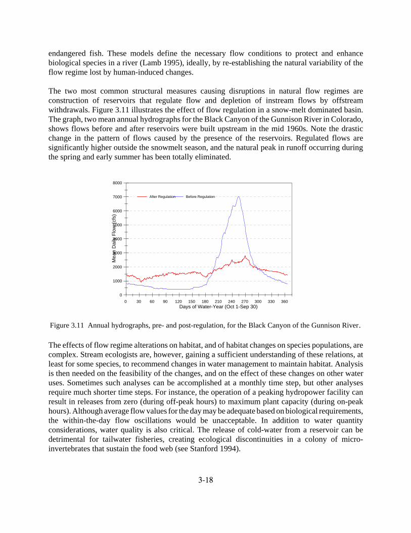
3-18

0

1000

2000

3000

4000

5000

6000

7000

8000

Mea

n D

aily

Flo

w (c

fs)

0 30 60 90 120 150 180 210 240 270 300 330 360 Days of Water-Year (Oct 1-Sep 30)

After Regulation Before Regulation

Figure 3.11 Annual hydrographs, pre- and post-regulation, for the Black Canyon of the Gunnison River.

endangered fish. These models define the necessary flow conditions to protect and enhancebiological species in a river (Lamb 1995), ideally, by re-establishing the natural variability of theflow regime lost by human-induced changes.

The two most common structural measures causing disruptions in natural flow regimes areconstruction of reservoirs that regulate flow and depletion of instream flows by offstreamwithdrawals. Figure 3.11 illustrates the effect of flow regulation in a snow-melt dominated basin.The graph, two mean annual hydrographs for the Black Canyon of the Gunnison River in Colorado,shows flows before and after reservoirs were built upstream in the mid 1960s. Note the drasticchange in the pattern of flows caused by the presence of the reservoirs. Regulated flows aresignificantly higher outside the snowmelt season, and the natural peak in runoff occurring duringthe spring and early summer has been totally eliminated.

The effects of flow regime alterations on habitat, and of habitat changes on species populations, arecomplex. Stream ecologists are, however, gaining a sufficient understanding of these relations, atleast for some species, to recommend changes in water management to maintain habitat. Analysisis then needed on the feasibility of the changes, and on the effect of these changes on other wateruses. Sometimes such analyses can be accomplished at a monthly time step, but other analysesrequire much shorter time steps. For instance, the operation of a peaking hydropower facility canresult in releases from zero (during off-peak hours) to maximum plant capacity (during on-peakhours). Although average flow values for the day may be adequate based on biological requirements,the within-the-day flow oscillations would be unacceptable. In addition to water quantityconsiderations, water quality is also critical. The release of cold-water from a reservoir can bedetrimental for tailwater fisheries, creating ecological discontinuities in a colony of micro-invertebrates that sustain the food web (see Stanford 1994).

3-19

Although economically significant fisheries are often identified, reliable estimation of nonuse andpreservation values in economic terms is not possible. Therefore, Aquarius does not assume thatdirect economic values for fish and wildlife habitat are available. This does not imply that thisparticular instream use of water has no economic value. Economic valuation research has confirmedthat the American public attaches significant value to wildlife and fish preservation (Boyle andBishop 1987), even though that value cannot be estimated with the same precision as other goodsand services. Although the public's willingness to pay for kilowatt-hours of electricity generated,tons of corn produced, and whitewater kayaking opportunities can be quantified, quantification ofthe economic value for the preservation of endangered species and similar environmental concernsfor direct incorporation in this model is insufficient.

What is proposed here is to address the water allocation problem for non-commensurate values ina unique manner. For a river site where the level of instream flow has been predetermined, but wherethe demand function in economic terms is difficult or impossible to define, the analyst canexperiment with fictitious demand curves until the required water allocation level for that instreamuse is satisfied. Indirectly, this approach indicates the societal willingness to pay for incrementalincreases of flow for difficult to value water uses. In other words, this approach estimates theeconomic subsidy required to sustain the activity in open competition with the other directly valueduses in the basin. Alternatively, the analyst has the option to impose minimum and maximuminstream flow requirements.

Despite the inherent limitation of the model that simulates monthly time-steps only, the capabilityof Aquarius to estimate the quantity and quality of habitat at one or several locations in a basin,along with the other water uses, should enable decision makers to evaluate the adverse effects ofplanned or existing water developments and water transfers and identify opportunities for mitigation,restoration, or enhancement of affected instream and riparian resources.

Flood Control

Flooding, the overflow of water onto normally dry land areas alongside a river orstream, can cause severe economic and human losses. Flood control is a commonobjective of reservoir management, but one often in conflict with other water usessuch as hydropower generation and instream flow requirements. The most generaloperational objective of flood-control for a flood prone area or river reach (FCA) is

to minimize the frequency and the magnitude of flood damages along the flood plain byimplementing a series of structural and non-structural control measures. Flood control optionsinclude flood abatement using upstream reservoirs, as well as channel management (dyking,channelizing) or land use controls (e.g., zoning) in areas subject to flooding (Leopold and Maddock,1954). Modeling flood control impacts in a river network can help one choose the most effectivecombination among those remediation alternatives.

Reservoirs, like natural lakes, can alter the frequency and magnitude of high and low flows (seehydrographs pre- and post-regulation in Figure 3.11). The ability of a reservoir to suppress flood

3-20

peaks depends largely on its storage capacity relative to the size of the catchment area, and on thereservoir’s operating rules. Flood control reservoirs with planned releases will diminish thefrequency of downstream overbank events. Often flooding risk can be further reduced by operatinga group of storage reservoirs as a system. However, reservoirs will rarely eliminate the risk ofdamage from very low frequency high flow events.

Unfortunately, the reduction in the frequency of overbank flooding resulting from reservoirmanagement of flows causes a deterioration of the channel’s natural capacity to handle flows, as theabsence of high peaks and flush floods allows sandbar deposition and vegetation encroachment intothe channel. The most common adjustment of the river to the new set of discharges and sedimentload reductions caused by the upstream reservoir is the formation of channel-in-channel sectionswith smaller bankfull discharge. This condition in turn exacerbates the flooding problem due to adecrease in channel capacity to convey high flows.

Nevertheless, protection from floods is a valuable service in many basins, and one that is likely togrow in importance due to population growth (there is continuous pressure for the reclamation offlood plains for urbanization) and the annexation of new agriculture land along the river banks.Moreover, as flow regulation lowers flood peaks in a river reach a false sense of security is createdamong inhabitants downstream from the flood control structures, who become unfamiliar withflooding and expect to be fully protected from all extreme events, further increasing the demand forflood control.

Access to the benefits of structural flood control measures cannot be restricted to specific users.Rather, once the structure is provided, the benefits are available to all individuals in the affectedflood plains. Also because access cannot be restricted, payment for the structures must be somehowshared by all beneficiaries. Typically, flood control structures are planned by government entitieswho use tax revenues or property assessments to finance construction and operation of the structures.Because of the public and nonexclusive nature of flood control, it is usually wise to analyze floodcontrol impacts and remedies over the entire basin.

Customarily, flood control benefits are estimated as the difference between expected flood damagesbefore and after mitigation measures are taken. James and Lee (1971, p.251) detail the procedureto estimate flood damages based on the severity of the floods. Direct damages are losses caused byphysical contact with the flood and are generally evaluated as the cost of replacing or rehabilitatingthe affected property in the case of urban damages (private and public) and as the net effect on farmincome in the case of crop damages. The distribution of flood damage potential within the floodplain may be summarized by a series of land-use maps each indicating the location of variousdevelopment classes (agricultural, residential, etc). A second series of maps indicates the severityof flooding throughout the flood plain for each flow level (flood stage). By superimposing each ofthe flood-severity maps over the land-use maps, flood damage as a function of water stage can bedetermined throughout the flood plain.

Marginal values for the economic assessment of flood control projects are usually expressed asfunctions of the frequency of the design flood. Rather than calculating the mathematical expectation

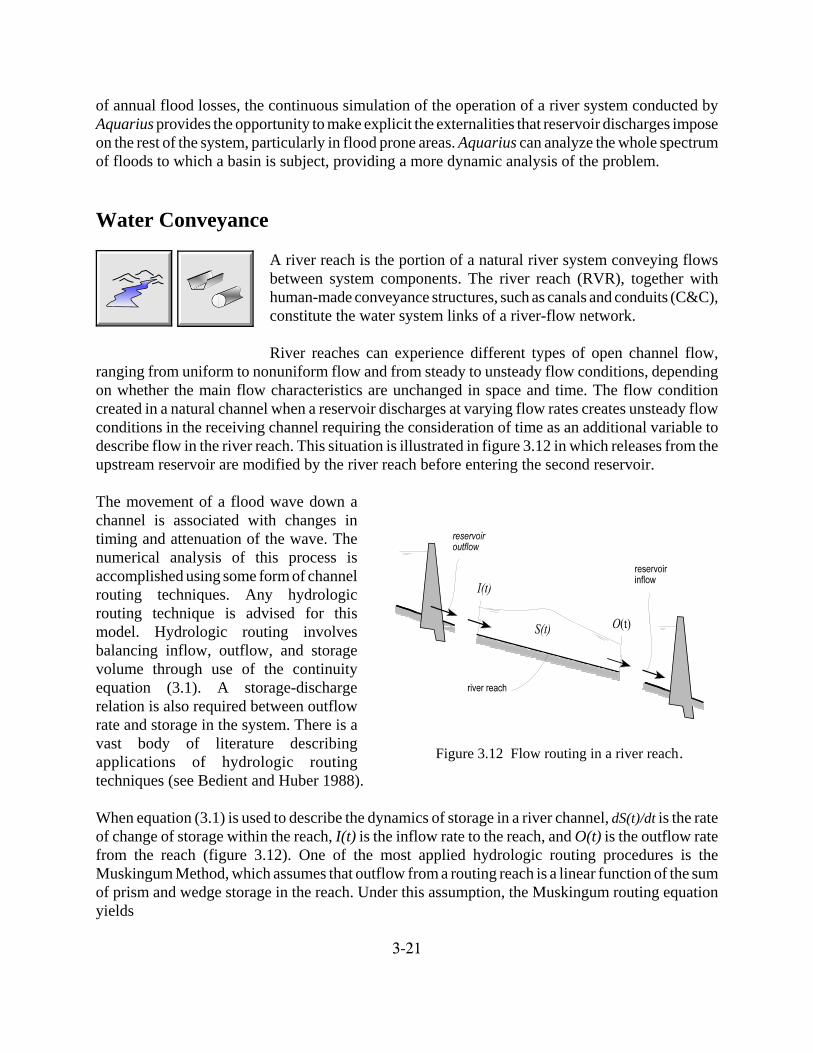
3-21

Figure 3.12 Flow routing in a river reach.

of annual flood losses, the continuous simulation of the operation of a river system conducted byAquarius provides the opportunity to make explicit the externalities that reservoir discharges imposeon the rest of the system, particularly in flood prone areas. Aquarius can analyze the whole spectrumof floods to which a basin is subject, providing a more dynamic analysis of the problem.

Water Conveyance

A river reach is the portion of a natural river system conveying flowsbetween system components. The river reach (RVR), together withhuman-made conveyance structures, such as canals and conduits (C&C),constitute the water system links of a river-flow network.

River reaches can experience different types of open channel flow,ranging from uniform to nonuniform flow and from steady to unsteady flow conditions, dependingon whether the main flow characteristics are unchanged in space and time. The flow conditioncreated in a natural channel when a reservoir discharges at varying flow rates creates unsteady flowconditions in the receiving channel requiring the consideration of time as an additional variable todescribe flow in the river reach. This situation is illustrated in figure 3.12 in which releases from theupstream reservoir are modified by the river reach before entering the second reservoir.

The movement of a flood wave down achannel is associated with changes intiming and attenuation of the wave. Thenumerical analysis of this process isaccomplished using some form of channelrouting techniques. Any hydrologicrouting technique is advised for thismodel. Hydrologic routing involvesbalancing inflow, outflow, and storagevolume through use of the continuityequation (3.1). A storage-dischargerelation is also required between outflowrate and storage in the system. There is avast body of literature describingapplications of hydrologic routingtechniques (see Bedient and Huber 1988).

When equation (3.1) is used to describe the dynamics of storage in a river channel, dS(t)/dt is the rateof change of storage within the reach, I(t) is the inflow rate to the reach, and O(t) is the outflow ratefrom the reach (figure 3.12). One of the most applied hydrologic routing procedures is theMuskingum Method, which assumes that outflow from a routing reach is a linear function of the sumof prism and wedge storage in the reach. Under this assumption, the Muskingum routing equationyields

3-22

(3.11)

Equation (3.11) indicates that the channel output at a given time step is a linear combination of theinflow to the reach during the same time step and the inflow and outflow during the previous timestep. The coefficients C1 , C2 , and C3 can be computed once the storage time constant for the reach“K” and the weighting factor “x”, the two Muskingum parameters, are known for the reach underconsideration.

The time required for a flood wave to traverse the reach dictates the need for routing procedures.When the water allocation problem is simulated using short time intervals of analysis (e.g., 24 hoursor less) streamflow routing is generally required to predict the temporal variations of a flood waveas it travels from the beginning to the end of the river reach. In contrast, when the time period ofanalysis is long (e.g., weekly or monthly periods) it is assumed that all water entering a river reachis available at the downstream end of the reach within the same time interval of simulation. Hence,channel routing procedures are unnecessary. This can be verified by knowing the length of the riverreach and a flow velocity for any representative flow rate.

Diversion and Junction

Water development projects may include other hydraulic structures inaddition to the conveyance structures (canals, pipelines) mentionedabove. For instance a water supply or irrigation project for which wateris drawn from a river and distributed to an urban area or irrigable landmay require the construction of a diversion dam across the river as to

maintain a water level high enough in the river to be able to always divert the required flow of water.The intake to the main canal may include an entrance structure with gates for controlling thedischarge into the canal. Alternatively, turnouts are used to divert relatively small volumes of waterfrom a supply watercourse to a smaller channel. The structure usually consists of an inlet, a conduitor a means or conveying water through the bank of the supply channel. Gates are usually used in theinlet to control the incoming flow. Aquarius can simulate flow diversions from either side of awatercourse, that is, left-bank and right-bank diversions (LBD and RBD, respectively).

Other water diversion schemes are developed for generating power at run-of-river hydroelectricplants (see fixed-head hydroplant in Figure 3.5). For instance, Figure 3.6 showed a portion of a flownetwork where hydropower is generated. It starts with a diversion node to divert water to thehydroplant, the feeding canal (diversion link), the power-house, a return link, and finishes with ajunction through which the same flow is returned to the stream. Aquarius can simulate flowjunctions with either side of a watercourse, that is, left-bank and right-bank junctions (LBJ and RBJ,respectively).

3-23

Aquarius considers any diversion node as a location in the flow network where a water allocationdecision should be made. A diversion link branching out of a node (see again at Figure 3.6) becomesa decision link when formulating the water allocation problem. In other words, the model convertsthe diversion link conveying water to a powerplant, an irrigation area or an urban water demandzone into a decision link and creates the corresponding set of decision variables.

Other Water Uses Not Included in the Model

The current version of the model provides the general framework and basic elements for the analysisof river networks. As future opportunities permit, additional water uses will be incorporated into themodel, allowing for a more comprehensive analysis of multipurpose water projects. Candidates forpossible future inclusion in the model include: (i) Instream Water Quality: changes in the physicaland chemical characteristics of instream flow are triggered by point and non-point pollution sourcesin the watershed. As surface flow levels are depleted, pollutants become concentrated and waterquality standards (e.g., dissolved oxygen level) may be violated. Enhancing instream flows provideseconomic benefits by mitigating the treatment cost that would be incurred by discharges and bydownstream water users to ensure compliance with federal and state standards (Young and Gray1972). (ii) Commercial River Navigation: commercial navigation requires sufficient flow to allowship passage. Instream flow needs for navigation may conflict with other water uses. For example,periodic fluctuations in reservoir releases from power peaking operations may disrupt navigation.