EFFICIENT RENDERING AND COMPRESSION

FOR

FULL-PARALLAX COMPUTER-GENERATED

HOLOGRAPHIC STEREOGRAMS

A Dissertation

Presented to the Faculty of the Graduate School

of Cornell University

in Partial Fulfillment of the Requirements for the Degree of

Doctor of Philosophy

by

Daniel Aaron Kartch

May 2000

c 2000 Daniel Aaron Kartch

ALL RIGHTS RESERVED

EFFICIENT RENDERING AND COMPRESSION

FOR

FULL-PARALLAX COMPUTER-GENERATED

HOLOGRAPHIC STEREOGRAMS

Daniel Aaron Kartch, Ph.D.

Cornell University 2000

In the past decade, we have witnessed a quantum leap in rendering technology

and a simultaneous increase in usage of computer generated images. Despite

the advances made thus far, we are faced with an ever increasing desire for

technology which can provide a more realistic, more immersive experience.

One fledgeling technology which shows great promise is the electronic holo-

graphic display. Holograms are capable of producing a fully three-dimensional

image, exhibiting all the depth cues of a real scene, including motion parallax,

binocular disparity, and focal effects. Furthermore, they can be viewed simulta-

neously by any number of users, without the aid of special headgear or position

trackers. However, to date, they have been limited in use because of their com-

putational intractability.

This thesis deals with the complex task of computing a hologram for use

with such a device. Specifically, we will focus on one particular type of holo-

gram: the holographic stereogram. A holographic stereogram is created by gen-

erating a large set of two-dimensional images of a scene as seen from multiple

camera points, and then converting them to a holographic interference pattern.

It is closely related to the light fields or lumigraphs used in image-based ren-

dering. Most previous algorithms have treated the problem of rendering these

images as independent computations, ignoring a great deal of coherency which

could be used to our advantage.

We present a new computationally efficient algorithm which operates on the

image set as a whole, rather than on its individual elements. Scene polygons are

mapped by perspective projection into a four-dimensional space, where they

are scan-converted into 4D color and depth buffers. We use a set of very simple

data structures and basic operations to form an algorithm which will lend itself

well to future hardware implementation, so as to drive a real-time holographic

display.

We also examined issues related to the compression of stereograms. Holo-

grams contain enormous amounts of data, which make storage and transmis-

sion cumbersome. We have derived new methods for efficiently compressing

this data. Results compare favorably with existing techniques.

Finally, we describe an algorithm for simulating a camera viewing a com-

puted hologram from arbitrary positions. It uses wave optics to track the prop-

agation of light from the hologram, through a lens, and onto a film plane. This

enabled us to evaluate our rendering and compression methods in the absence

of an electronic holographic display and without the lengthy processing time of

hardcopy holographic printing.

Biographical Sketch

Dan Kartch was born in Pompton Plains, NJ on January 4, 1967, and was raised

in Wayne, NJ. After graduating from Wayne Hills High School in 1985, he at-

tended Cornell University in Ithaca, NY, where he majored in Physics. There,

he received his first experience in computer graphics while working for as-

tronomers Saul Teukolsky and Stuart Shapiro, producing videos of the results

of their research. After receiving a B.A. in 1989, he remained at Cornell to study

under Donald Greenberg in the Program of Computer Graphics. Several hun-

dred years later, he produced the volume you are now holding, and received

his Ph.D. in Computer Science.

iii

To my parents.

iv

Acknowledgements

First and foremost, I would like to thank my committee chair, Donald Green-

berg. Don was undetered by the forward-looking nature of my research, and

the fact that, even if successful, it would not prove to be practically applicable

for several years after its completion, until various other technological advance-

ments are achieved. He continued to provide advice and support, both moral

and financial, despite the many, many, many, many, many, many years that it

took me to finish. For this, I will always be grateful.

I would also like to thank the other members of my committee, Ken Tor-

rance and Saul Teukolsky, for their continuing support. I am especially grate-

ful to Saul, as well as Stuart Shapiro, who gave me a part-time job performing

graphics programming during my junior and senior years as an undergradu-

ate. It was there that computer programming, which had previously been only

a hobby for me, grew to become a career. I also thank Jack Tumblin for his

services as reviewer and proofreader.

I thank my parents, Matthew and Joan Kartch, my brother David, and many

friends from my days as an undergraduate, whose constant nagging, er : : : I

mean whose steadfast encouragement, helped me see my degree through to

completion.

v

I thank Ben Trumbore for providing me with a place to live for most of my

time in graduate school, and for serving as an avid and challenging opponent

in games too numerous to count. On a similar note, I must thank Chris Schoen-

eman for providing an incredibly evil bit of software that wasted much valu-

able time which would have been better spent working, and also Gun Alppay,

Sebastian Fernandez, Gene Greger, Andrew Kunz, Jed Lengyel, Brian Smits,

Greg Spencer, Bretton Wade, and anyone else I may have forgotten, all of whom

blowed up real good.

I am grateful to the following people who provided software or services

which were invaluable during my research: our system administrators, Hurf

Sheldon and Mitch Collinsworth, who kept everything running (most of the

time); James Durkin, who provided support for Emacs and various other utili-

ties; Bruce Walter, for his RGBE libraries and for generating a global illumina-

tion solution used in this thesis; Moreno Piccolotto and SuAnne Fu, for their aid

in preparing several of the models used here, and Richard Meier Associates for

providing one of those models to us; Pete Shirley, whose gg libraries saved me

a lot of bother; and the consultants of the Cornell Theory Center for aiding me

with various problems. I thank the contributors to several software projects for

selflessly making the fruits of their efforts free to all and sundry: LaTeX, GNU

Emacs, MPICH, FFTW, ImageMagick, and the GIMP. Similarly, I thank the fol-

lowing people who made their models available on the web: Barry Driessen,

Dave Edwards, and Luis Filipe.

My thanks go out as well to the many other staff and students in the lab who

have made my stay at Cornell so pleasant.

Last but not least, I am grateful to the various sponsors without whose sup-

vi

port this research would not have been possible. This work was supported in

part by the National Science Foundation Science and Technology Center for

Computer Graphics and Scientific Visualization (ASC-8920219), and by NSF

grants ASC-9523483 and CCR-8617880. Much of this research was performed

on equipment generously donated by the Hewlett-Packard Corporation and the

Intel Corporation. I also thank the Cornell Theory Center, which receives fund-

ing from Cornell University, New York State, federal agencies, and corporate

partners, for the use of their computing resources.

vii

Table of Contents

Biographical Sketch . . . . . . . . . . . . . . . . . . . . . . . . . . . . . . iiiDedication . . . . . . . . . . . . . . . . . . . . . . . . . . . . . . . . . . . ivAcknowledgements . . . . . . . . . . . . . . . . . . . . . . . . . . . . . . vTable of Contents . . . . . . . . . . . . . . . . . . . . . . . . . . . . . . . viiiList of Figures . . . . . . . . . . . . . . . . . . . . . . . . . . . . . . . . . xi

1 Introduction 1

2 Three-Dimensional Displays 42.1 The need for a three-dimensional display . . . . . . . . . . . . . . 52.2 Stereoscopic displays . . . . . . . . . . . . . . . . . . . . . . . . . . 8

2.2.1 Liquid-crystal shutter systems . . . . . . . . . . . . . . . . 92.2.2 Chromostereoscopy . . . . . . . . . . . . . . . . . . . . . . 132.2.3 Head-mounted displays . . . . . . . . . . . . . . . . . . . . 152.2.4 Autostereoscopic displays . . . . . . . . . . . . . . . . . . . 162.2.5 Stereoblindness . . . . . . . . . . . . . . . . . . . . . . . . . 18

2.3 Direct volume displays . . . . . . . . . . . . . . . . . . . . . . . . . 182.3.1 Varifocal mirror displays . . . . . . . . . . . . . . . . . . . 192.3.2 Rotating screen displays . . . . . . . . . . . . . . . . . . . . 19

2.4 Holographic displays . . . . . . . . . . . . . . . . . . . . . . . . . . 21

3 Computer-Generated Holography 223.1 Notation . . . . . . . . . . . . . . . . . . . . . . . . . . . . . . . . . 253.2 Problem definition . . . . . . . . . . . . . . . . . . . . . . . . . . . 263.3 Geometric simplifications . . . . . . . . . . . . . . . . . . . . . . . 303.4 Fourier holography . . . . . . . . . . . . . . . . . . . . . . . . . . . 31

3.4.1 Fraunhofer holograms . . . . . . . . . . . . . . . . . . . . . 323.4.2 Fresnel holograms . . . . . . . . . . . . . . . . . . . . . . . 343.4.3 Image plane Fourier holograms . . . . . . . . . . . . . . . . 38

3.5 Horizontal parallax only holograms . . . . . . . . . . . . . . . . . 393.6 Holographic stereograms . . . . . . . . . . . . . . . . . . . . . . . 423.7 Diffraction specific computation . . . . . . . . . . . . . . . . . . . 44

3.7.1 Lumigraph . . . . . . . . . . . . . . . . . . . . . . . . . . . 453.7.2 Hogel representation . . . . . . . . . . . . . . . . . . . . . . 473.7.3 Conversion to an interference pattern . . . . . . . . . . . . 50

viii

3.7.4 Hogel basis functions . . . . . . . . . . . . . . . . . . . . . 53

4 Representation and Compression 564.1 Sampling domain . . . . . . . . . . . . . . . . . . . . . . . . . . . . 594.2 Transforms . . . . . . . . . . . . . . . . . . . . . . . . . . . . . . . . 61

4.2.1 Windowed discrete cosine transform . . . . . . . . . . . . . 624.2.2 Wavelets . . . . . . . . . . . . . . . . . . . . . . . . . . . . . 634.2.3 Applying transforms in higher dimensions . . . . . . . . . 64

4.3 Entropy Coding . . . . . . . . . . . . . . . . . . . . . . . . . . . . . 694.4 Quantization and Symbol Generation . . . . . . . . . . . . . . . . 71

4.4.1 JPEG-based encoding . . . . . . . . . . . . . . . . . . . . . 714.4.2 Wavelet encoding . . . . . . . . . . . . . . . . . . . . . . . . 73

4.5 Results . . . . . . . . . . . . . . . . . . . . . . . . . . . . . . . . . . 804.5.1 Error metric . . . . . . . . . . . . . . . . . . . . . . . . . . . 804.5.2 Compression metric . . . . . . . . . . . . . . . . . . . . . . 814.5.3 Results . . . . . . . . . . . . . . . . . . . . . . . . . . . . . . 82

5 Rendering 955.1 Generalized Lumigraph Rendering . . . . . . . . . . . . . . . . . . 965.2 Previous Work . . . . . . . . . . . . . . . . . . . . . . . . . . . . . . 99

5.2.1 Ray Tracing . . . . . . . . . . . . . . . . . . . . . . . . . . . 995.2.2 2D Rendering . . . . . . . . . . . . . . . . . . . . . . . . . . 1005.2.3 Multiple Viewpoint Rendering . . . . . . . . . . . . . . . . 103

5.3 Proposed Algorithm . . . . . . . . . . . . . . . . . . . . . . . . . . 1055.4 Projected Volume . . . . . . . . . . . . . . . . . . . . . . . . . . . . 1075.5 Homogeneous Projected Volume . . . . . . . . . . . . . . . . . . . 1115.6 Simplices and Simploids . . . . . . . . . . . . . . . . . . . . . . . . 115

5.6.1 Subdivision of a simploid . . . . . . . . . . . . . . . . . . . 1185.6.2 Clipping and slicing a simplex . . . . . . . . . . . . . . . . 118

5.7 Complete Algorithm . . . . . . . . . . . . . . . . . . . . . . . . . . 1215.7.1 Projection / Back-face culling . . . . . . . . . . . . . . . . . 1215.7.2 Clipping . . . . . . . . . . . . . . . . . . . . . . . . . . . . . 1235.7.3 Scanning in U and V . . . . . . . . . . . . . . . . . . . . . . 1255.7.4 Scanning in s and t . . . . . . . . . . . . . . . . . . . . . . . 125

5.8 Results . . . . . . . . . . . . . . . . . . . . . . . . . . . . . . . . . . 128

6 Holographic Image Preview 1376.1 Projection . . . . . . . . . . . . . . . . . . . . . . . . . . . . . . . . . 138

6.1.1 Translation . . . . . . . . . . . . . . . . . . . . . . . . . . . . 1396.1.2 Rotation . . . . . . . . . . . . . . . . . . . . . . . . . . . . . 1426.1.3 Direction restriction . . . . . . . . . . . . . . . . . . . . . . 143

6.2 Focus . . . . . . . . . . . . . . . . . . . . . . . . . . . . . . . . . . . 1456.3 Exposure . . . . . . . . . . . . . . . . . . . . . . . . . . . . . . . . . 1476.4 Results . . . . . . . . . . . . . . . . . . . . . . . . . . . . . . . . . . 147

ix

7 Conclusions 1507.1 Summary . . . . . . . . . . . . . . . . . . . . . . . . . . . . . . . . . 1507.2 Comments and Future Work . . . . . . . . . . . . . . . . . . . . . . 151

7.2.1 Compression . . . . . . . . . . . . . . . . . . . . . . . . . . 1517.2.2 Rendering . . . . . . . . . . . . . . . . . . . . . . . . . . . . 153

7.3 Final Thoughts . . . . . . . . . . . . . . . . . . . . . . . . . . . . . 154

Bibliography 156

x

List of Figures

2.1 Stereoscopes, then and now . . . . . . . . . . . . . . . . . . . . . . 82.2 Stereoscope function . . . . . . . . . . . . . . . . . . . . . . . . . . 92.3 Eclipse projection system . . . . . . . . . . . . . . . . . . . . . . . 102.4 Polarizing stereo projection system . . . . . . . . . . . . . . . . . 122.5 Superchromatic prism . . . . . . . . . . . . . . . . . . . . . . . . . 142.6 Chromostereoscopic glasses . . . . . . . . . . . . . . . . . . . . . . 142.7 Parallax barrier . . . . . . . . . . . . . . . . . . . . . . . . . . . . . 162.8 Lenticular sheet . . . . . . . . . . . . . . . . . . . . . . . . . . . . . 172.9 Varifocal mirror . . . . . . . . . . . . . . . . . . . . . . . . . . . . . 192.10 Rotating screen displays . . . . . . . . . . . . . . . . . . . . . . . . 20

3.1 Sample scene . . . . . . . . . . . . . . . . . . . . . . . . . . . . . . 263.2 Sampling and maximum viewing angle . . . . . . . . . . . . . . . 283.3 Scene with objects replaced by point sources . . . . . . . . . . . . 303.4 Scene with objects replaced by line sources . . . . . . . . . . . . . 313.5 Fraunhofer hologram . . . . . . . . . . . . . . . . . . . . . . . . . 323.6 Repetition in a Fourier holograms . . . . . . . . . . . . . . . . . . 353.7 Fresnel hologram with multiple objects . . . . . . . . . . . . . . . 363.8 HPO hologram formation . . . . . . . . . . . . . . . . . . . . . . . 403.9 HPO hologram reconstruction . . . . . . . . . . . . . . . . . . . . 403.10 Holographic stereogram . . . . . . . . . . . . . . . . . . . . . . . . 433.11 Light field / lumigraph . . . . . . . . . . . . . . . . . . . . . . . . 463.12 Hogel . . . . . . . . . . . . . . . . . . . . . . . . . . . . . . . . . . 483.13 Limits on hogel resolution . . . . . . . . . . . . . . . . . . . . . . . 493.14 Light received from hogel . . . . . . . . . . . . . . . . . . . . . . . 513.15 Correspondence between frequency space and direction . . . . . 523.16 Lucente’s basis functions . . . . . . . . . . . . . . . . . . . . . . . 54

4.1 Lumigraph compression and conversion . . . . . . . . . . . . . . 574.2 Frequency space discretization of hemisphere . . . . . . . . . . . 604.3 Hemicube . . . . . . . . . . . . . . . . . . . . . . . . . . . . . . . . 624.4 DCT basis functions . . . . . . . . . . . . . . . . . . . . . . . . . . 634.5 Daubechies orthonormal wavelets . . . . . . . . . . . . . . . . . . 654.6 Average-interpolating wavelets . . . . . . . . . . . . . . . . . . . 654.7 Interpolating wavelets . . . . . . . . . . . . . . . . . . . . . . . . . 65

xi

4.8 CDF biorthogonal wavelets . . . . . . . . . . . . . . . . . . . . . . 654.9 (9,7) wavelet . . . . . . . . . . . . . . . . . . . . . . . . . . . . . . . 654.10 Hemicube separation . . . . . . . . . . . . . . . . . . . . . . . . . 674.11 Hemicube unfolding . . . . . . . . . . . . . . . . . . . . . . . . . . 684.12 Entropy coding . . . . . . . . . . . . . . . . . . . . . . . . . . . . . 704.13 Sample JPEG quantization table . . . . . . . . . . . . . . . . . . . 714.14 JPEG block traversal . . . . . . . . . . . . . . . . . . . . . . . . . . 734.15 Wavelet coefficient hierarchy . . . . . . . . . . . . . . . . . . . . . 744.16 EZW encoding example . . . . . . . . . . . . . . . . . . . . . . . . 754.17 3-pass encoding example . . . . . . . . . . . . . . . . . . . . . . . 784.18 EZW vs. 3-pass . . . . . . . . . . . . . . . . . . . . . . . . . . . . . 804.19 Jack-o-lantern compression graph . . . . . . . . . . . . . . . . . . 854.20 Church compression examples . . . . . . . . . . . . . . . . . . . . 854.21 Jack-o-lantern compression examples . . . . . . . . . . . . . . . . 864.22 Jack-o-lantern compression examples (cont.) . . . . . . . . . . . . 874.23 Jack-o-lantern compression examples (cont.) . . . . . . . . . . . . 884.24 Jack-o-lantern compression examples (cont.) . . . . . . . . . . . . 894.25 Church compression examples . . . . . . . . . . . . . . . . . . . . 904.26 Church compression examples (cont.) . . . . . . . . . . . . . . . . 914.27 Church compression examples (cont.) . . . . . . . . . . . . . . . . 924.28 Church compression examples (cont.) . . . . . . . . . . . . . . . . 934.29 Example of different levels of compression . . . . . . . . . . . . . 94

5.1 Lumigraph parameterization . . . . . . . . . . . . . . . . . . . . . 965.2 Lumigraph of a single triangular polygon . . . . . . . . . . . . . . 985.3 Four perspective views of triangle . . . . . . . . . . . . . . . . . . 985.4 Triangle’s projected volume . . . . . . . . . . . . . . . . . . . . . . 985.5 Lumigraph computation with ray-tracing . . . . . . . . . . . . . . 1005.6 Lumigraph computation with 2D renderer . . . . . . . . . . . . . 1015.7 Lumigraph computation with 2D z-buffer . . . . . . . . . . . . . 1025.8 Halle’s MVR algorithm . . . . . . . . . . . . . . . . . . . . . . . . 1045.9 Brief outline of new algorithm . . . . . . . . . . . . . . . . . . . . 1065.10 Projected volume of triangular polygon and triangular lumigraph 1095.11 Edges of projected volume . . . . . . . . . . . . . . . . . . . . . . 1105.12 Faces of projected volume . . . . . . . . . . . . . . . . . . . . . . . 1105.13 Hyperfaces of projected volume . . . . . . . . . . . . . . . . . . . 1105.14 Back- and front-face lobes in projected volume . . . . . . . . . . . 1145.15 Simplices . . . . . . . . . . . . . . . . . . . . . . . . . . . . . . . . 1165.16 Simploids . . . . . . . . . . . . . . . . . . . . . . . . . . . . . . . . 1175.17 Subdividing simploids into 4-simplices . . . . . . . . . . . . . . . 1195.18 Clipping 4-simplices . . . . . . . . . . . . . . . . . . . . . . . . . . 1205.19 Slicing a 4-simplex . . . . . . . . . . . . . . . . . . . . . . . . . . . 1215.20 Slicing a 3-simplex . . . . . . . . . . . . . . . . . . . . . . . . . . . 1215.21 Full algorithm . . . . . . . . . . . . . . . . . . . . . . . . . . . . . . 122

xii

5.22 Back-face culling . . . . . . . . . . . . . . . . . . . . . . . . . . . . 1245.23 Conversion from (S; T ) to (s; t) . . . . . . . . . . . . . . . . . . . . 1265.24 Curves in (s; t) . . . . . . . . . . . . . . . . . . . . . . . . . . . . . 1265.25 Scanning in (s; t) . . . . . . . . . . . . . . . . . . . . . . . . . . . . 1265.26 Times for church model (direct illumination) . . . . . . . . . . . . 1325.27 Times for church model (global illumination) . . . . . . . . . . . . 1335.28 Times for chandelier . . . . . . . . . . . . . . . . . . . . . . . . . . 1345.29 Times for pool table . . . . . . . . . . . . . . . . . . . . . . . . . . 1355.30 Times for jack-o-lantern . . . . . . . . . . . . . . . . . . . . . . . . 136

6.1 Camera model overview . . . . . . . . . . . . . . . . . . . . . . . 1386.2 Field generated by a hologram . . . . . . . . . . . . . . . . . . . . 1396.3 Projecting between parallel planes . . . . . . . . . . . . . . . . . . 1406.4 Decomposition of light field . . . . . . . . . . . . . . . . . . . . . . 1406.5 Basic projection . . . . . . . . . . . . . . . . . . . . . . . . . . . . . 1426.6 Projection between arbitrary planes . . . . . . . . . . . . . . . . . 1436.7 Projection with rotation . . . . . . . . . . . . . . . . . . . . . . . . 1436.8 Limits of propagation directions . . . . . . . . . . . . . . . . . . . 1446.9 Projection with limited directions . . . . . . . . . . . . . . . . . . 1446.10 Focusing by a thin lens . . . . . . . . . . . . . . . . . . . . . . . . 1456.11 Test model . . . . . . . . . . . . . . . . . . . . . . . . . . . . . . . . 1486.12 Test of camera simulator . . . . . . . . . . . . . . . . . . . . . . . . 149

xiii

Chapter 1

Introduction

Twenty years ago, the computer was seen by most people as a mysterious and

daunting device whose use was relegated to an elite few capable of mastering

the arcane languages and rituals needed to invoke it. Today, it has become an

indispensable tool in almost all walks of life, and is revolutionizing the fields of

engineering, medicine, and scientific research. Its success is due in large part to

the development of fast graphics hardware and software which enable users to

interact with their data and designs at an easily comprehensible visual level.

However, as the data to be dealt with becomes more and more complex, we

see increasing dissatisfaction with the limitations of standard two-dimensional

display systems. No matter how fast or photo-realistic the output of rendering

software becomes, it cannot take full advantage of the human visual system’s

capabilities so long as the results can only be viewed on a flat screen. To meet

this need, a great deal of research has been dedicated to the development of

three-dimensional display systems. A number of devices based on several dif-

ferent display methods are already commercially available, and work continues

on improving these technologies and developing new ones.

1

2

One of the most promising is the electronic holographic display. A holo-

graphic display would be able to produce a completely realistic three-dimen-

sional image of an object or scene without the need for special eyewear or po-

sition trackers. It could therefore be viewed simultaneously from any angle by

any number of users.

This functionality does not come cheap. A holographic display requires a

resolution several orders of magnitude higher than that of a CRT monitor. The

current state of the art can provide small screens with this resolution in only one

dimension, allowing the display of holograms with limited parallax and depth.

It may be a decade or more before full-size, full-parallax holographic monitors

become a commercial reality, but researchers are confident that this goal will be

achieved.

In addition to the engineering obstacles that must be overcome, there are

computational hurdles as well. Simulating the optical phenomena that produce

a hologram is a much more complex problem than that which produces a two-

dimensional image. Furthermore, where a typical computer-generated image

requires a few million bytes of information, a hologram requires hundreds of

billions or more. Not only does this present an enormous computation task, it

is also a tremendous amount of data to be stored or transmitted to the display

device. There is therefore a great need for algorithms to efficiently compute and

compress holograms.

The most promising methods we have seen are those based on a class of

hologram known as holographic stereograms, particularly the work on diffrac-

tion specific computation performed by Lucente at the MIT Media Lab. These

methods will be discussed in detail later. For now we summarize by saying

3

that they split the computation into two stages. In the first stage, a set of two-

dimensional images are generated using traditional rendering algorithms. In

the second stage, these images are converted into a holographic interference pat-

tern using Fourier techniques. These methods provide a tremendous increase

in speed over single step algorithms which produce a hologram directly from

a scene by simulating the interference which would occur in the real world. In

addition, as Lucente showed, the images produced by the first stage can serve

as a far better compression domain than the interference patterns, and using

specialized hardware, we can rapidly convert from this compressed form to the

final hologram.

In this thesis, we build upon this work, improving computation speed and

compression statistics. Unlike much of the previous work , which focused pri-

marily on horizontal parallax only holograms, we will look at the more general,

and more computationally complex, case of full-parallax holograms. Chapter

2 provides an overview of three-dimensional display technology and discusses

the advantages of a holographic display. Chapter 3 discusses previous work in

computational holography. Chapter 4 proposes and compares several compres-

sion schemes. Chapter 5 presents a four-dimensional z-buffering algorithm for

rapidly performing the rendering process. Chapter 6 describes a method for

testing holographic rendering algorithms in the absence of an electronic holo-

graphic display to provide visual feedback. Chapter 7 concludes by summariz-

ing our results and discussing avenues for future research.

Chapter 2

Three-Dimensional Displays

As mentioned in the previous chapter, the development of a holographic dis-

play is not a simple task. Why then, should we bother when existing tech-

nologies such as stereoscopic monitors and virtual reality headsets can already

produce convincing three-dimensional effects? When we first undertook this

project, we heard many questions along these lines. In order to motivate this

work and answer these questions, this chapter provides a brief overview of

past and present 3D display devices, and discusses their relative advantages

and disadvantages.

Three-dimensional display devices have a long history, dating back to the

first half of the nineteenth century. Okoshi [94, 95] and Lipton [75] provide ex-

tensive explanations and historical discussions of three-dimensional imaging

techniques prior to 1980. McAllister et al. [88] describe current electronic 3D

display devices and their use with computer generated images.

4

5

2.1 The need for a three-dimensional display

Our visual system transforms the two-dimensional images received by our eyes

into a three-dimensional representation of the world using a combination of

psychological and physiological depth cues [56]. The psychological cues are

primarily functions of how the environment projects onto our retina. Examples

include linear perspective, texture gradient, retinal image size, aerial perspec-

tive, relative brightness, shading, and occlusion. The physiological depth cues

are functions of how our eyes adjust to view objects at different distances and

how the images change when viewed from different positions. These include

the focal length and convergence of the eyes, binocular disparity, and motion

parallax.

Using perspective transformations, hidden surface removal, texture map-

ping, global illumination algorithms, and good reflection models, we can create

computer generated images that provide all of the psychological depth cues.

While we cannot yet produce perfectly photo-realistic images of arbitrary

scenes, the differences affect the realism of the images, not their three-dimen-

sionality. However, when we view a two dimensional image, we are focusing

on a fixed object (the monitor or photograph) at a single depth. This depth is

unaffected by what point in the image we look at, or how distant an object that

part of the image represents, and therefore the physiological depth cues are not

present.

In most cases, psychological depth cues are sufficient. However, for a grow-

ing set of applications, additional cues are needed to interpret the information

being displayed. To illustrate, we will take a look at examples of three classes of

applications where this is the case.

6

Applications where the display must match reality as closely as possible:

Flight simulators are becoming increasingly important for the training of mil-

itary and airline pilots. They allow difficult maneuvers to be learned, and test

reactions in dangerous situations, without risk to life or property. Since the en-

vironments for which the pilots are training provide physiological depth cues, it

is important that the simulations provide them as well. Otherwise, the percep-

tual changes when going from the simulator to the real world may slow reaction

time and lead to fatal mistakes.

Applications where psychological depth cues are present but useless: Our

visual system’s use of psychological depth cues is adapted to deal with envi-

ronments normally encountered in the real world, and can fail when we are

placed in highly atypical surroundings. If placed in a room whose dimensions

have been deliberately distorted to project the same image on the retina as a

normal room while actually being quite different, we will interpret the scene as

the more familiar environment, rather than as it truly is. If placed in an envi-

ronment that does not resemble anything we have ever encountered, we will

have a hard time interpreting it at all. Scientific data sets provide just such an

environment. We do not encounter complex molecular chains or colored clouds

representing electrical potentials in our normal visual world, and therefore have

difficulty understanding them when displayed on a monitor, no matter how re-

alistically they are rendered. A three-dimensional display radically improves

this situation. The addition of physiological depth cues causes coherent struc-

tures in the data to be immediately apparent to the user, greatly increasing the

usefulness of scientific visualization software.

7

Applications where psychological depth cues are absent or undesirable:

Consider the design of an air traffic control system. The controllers need to be

able to monitor the paths of multiple, widely-separated objects through a mostly

empty three-dimensional space. Because this environment is so sparse, the

dominant psychological depth cues which would be available in a realistic ren-

dering would be the retinal image size and aerial perspective. These, however,

are undesirable in this situation, because they would make it difficult for con-

trollers to see distant airplanes. Instead, they are forced to use two-dimensional

abstractions with image position representing map coordinates and height in-

dicated by textual annotations. These displays require some experience to use

since it is difficult to determine from a 2D image whether or not two airplanes in

the 3D space will come close enough for there to be a danger of collision. What

is really needed here is a three-dimensional display which the controller can

view from any angle, easily and accurately determining the relative positions

and paths of every plane.

As these three cases illustrate, there is a growing class of applications for

which ordinary two-dimensional displays are inadequate. The depth cues they

provide are insufficient to allow the user to easily and naturally interpret the

scenes being rendered. With the introduction of a three-dimensional display,

these problems can be overcome. In addition, Merrit [91] lists several other side-

benefits of 3D displays: they aid in filtering visual noise and provide greater

effective image quality; they provide a wider total field of view; and they allow

the display of luster, scintillation, and surface sheen (which are highly depen-

dent on viewing position), improving the realism of images.

8

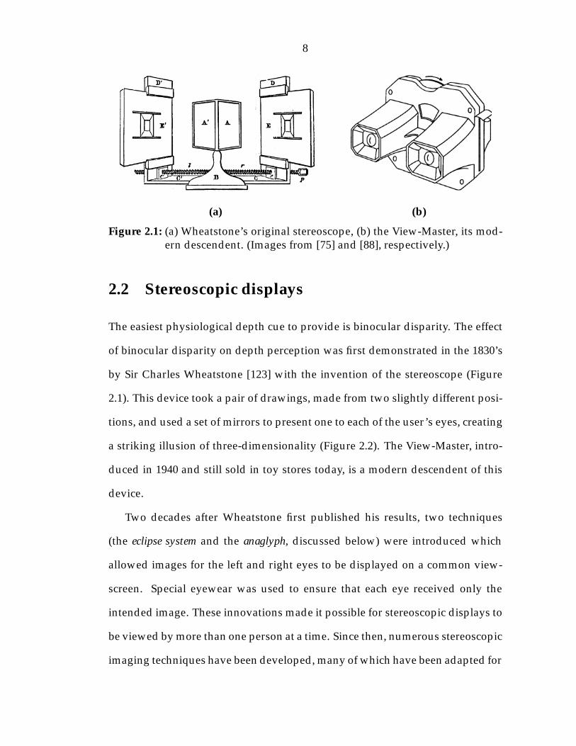
(a) (b)

Figure 2.1: (a) Wheatstone’s original stereoscope, (b) the View-Master, its mod-ern descendent. (Images from [75] and [88], respectively.)

2.2 Stereoscopic displays

The easiest physiological depth cue to provide is binocular disparity. The effect

of binocular disparity on depth perception was first demonstrated in the 1830’s

by Sir Charles Wheatstone [123] with the invention of the stereoscope (Figure

2.1). This device took a pair of drawings, made from two slightly different posi-

tions, and used a set of mirrors to present one to each of the user’s eyes, creating

a striking illusion of three-dimensionality (Figure 2.2). The View-Master, intro-

duced in 1940 and still sold in toy stores today, is a modern descendent of this

device.

Two decades after Wheatstone first published his results, two techniques

(the eclipse system and the anaglyph, discussed below) were introduced which

allowed images for the left and right eyes to be displayed on a common view-

screen. Special eyewear was used to ensure that each eye received only the

intended image. These innovations made it possible for stereoscopic displays to

be viewed by more than one person at a time. Since then, numerous stereoscopic

imaging techniques have been developed, many of which have been adapted for

9

MirrorsL

efti

mag

e

Rightim

age(a) Wheatstone’s stereoscope

Left image Right image

(b) View-Master

Figure 2.2: Schematics of the devices in Figure 2.1. The mirrors / lenses areadjusted so that the images appear in a natural viewing position.The left and right eye images are fused by the human visual systemto create an illusion of three-dimensionality.

electronic displays.

2.2.1 Liquid-crystal shutter systems

Passive screen, active glasses

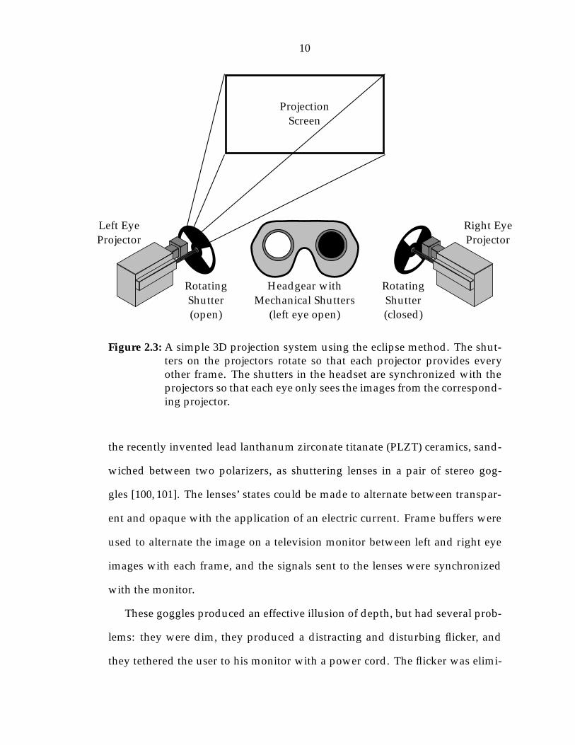
One of the most popular stereo display methods is an adaptation of the eclipse

system (Figure 2.3). According to Lipton [78], this system was invented in 1858,

and first used commercially by Laurens Hammond in 1922. Images for the left

and right eyes are projected in alternation onto a single screen. The user views

the screen through headgear containing shutters for each eye. The shutters open

and close in synchronization with the projectors so that the left eye sees one set

of images and the right sees the other.

Numerous mechanical and electrical shuttering systems have been devel-

oped since then, but none could be made commercially feasible until modern

electro-optical materials were developed. In the mid-70’s, John Roese used

10

Left EyeProjector

Right EyeProjector

RotatingShutter(open)

RotatingShutter(closed)

ProjectionScreen

Headgear withMechanical Shutters

(left eye open)

Figure 2.3: A simple 3D projection system using the eclipse method. The shut-ters on the projectors rotate so that each projector provides everyother frame. The shutters in the headset are synchronized with theprojectors so that each eye only sees the images from the correspond-ing projector.

the recently invented lead lanthanum zirconate titanate (PLZT) ceramics, sand-

wiched between two polarizers, as shuttering lenses in a pair of stereo gog-

gles [100, 101]. The lenses’ states could be made to alternate between transpar-

ent and opaque with the application of an electric current. Frame buffers were

used to alternate the image on a television monitor between left and right eye

images with each frame, and the signals sent to the lenses were synchronized

with the monitor.

These goggles produced an effective illusion of depth, but had several prob-

lems: they were dim, they produced a distracting and disturbing flicker, and

they tethered the user to his monitor with a power cord. The flicker was elimi-

11

nated with the introduction [80] of a 120 Hz monitor. The dimness was solved

by replacing the PLZT with liquid-crystal (LC) shutters [51], which provided

much higher transparency. The LC shutters also drew much less power, allow-

ing the power cord to be eliminated in favor of a battery in the glasses [77]. Syn-

chronization of the shutters with the display was now provided by an infrared

emitter mounted atop the monitor. StereoGraphics has been quite successful

marketing this device under the brand name CrystalEyes [109].

Active screen, passive glasses

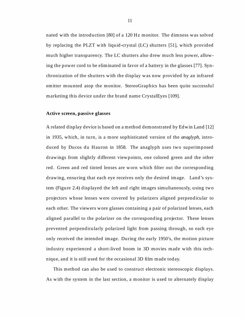
A related display device is based on a method demonstrated by Edwin Land [12]

in 1935, which, in turn, is a more sophisticated version of the anaglyph, intro-

duced by Ducos du Hauron in 1858. The anaglyph uses two superimposed

drawings from slightly different viewpoints, one colored green and the other

red. Green and red tinted lenses are worn which filter out the corresponding

drawing, ensuring that each eye receives only the desired image. Land’s sys-

tem (Figure 2.4) displayed the left and right images simultaneously, using two

projectors whose lenses were covered by polarizers aligned perpendicular to

each other. The viewers wore glasses containing a pair of polarized lenses, each

aligned parallel to the polarizer on the corresponding projector. These lenses

prevented perpendicularly polarized light from passing through, so each eye

only received the intended image. During the early 1950’s, the motion picture

industry experienced a short-lived boom in 3D movies made with this tech-

nique, and it is still used for the occasional 3D film made today.

This method can also be used to construct electronic stereoscopic displays.

As with the system in the last section, a monitor is used to alternately display

12

Left EyeProjector

Right EyeProjector

HorizontalPolarizer

VerticalPolarizer

ProjectionScreen

Glasses withPerpendicular Polarizers

Figure 2.4: Land’s stereoscopic projection system. The projectors produce twoperpendicularly polarized images on the viewscreen. The polarizedglasses filter out the appropriate image for each eye.

right and left images. Instead of a shutter mechanism built into the lenses, the

monitor is covered with a transparent liquid-crystal screen whose polarization

alternates between vertical and horizontal in sync with the monitor [79]. The

user now wears only a simple and inexpensive pair of polarized lenses. The

large polarized screen is more expensive to make than the LC shutter glasses,

but is becoming more cost effective with the introduction of new LCD technol-

ogy, especially in situations where the display is to be seen by many viewers at

once, such as with a large projection-screen display [76].

13

Common characteristics of LC shutter displays

These displays allow affordable, three-dimensional viewing for multiple users.

However, they have several disadvantages. First, they only provide a proper

image of the environment for a single viewing position. Looking at the monitor

from a different position causes the image to appear oddly sheared. The addi-

tion of a head-mounted position tracker [1,92] fixes this problem, but the image

will still only be optimized for a single viewer. Second, the rapid switching

back and forth between the two eyes, as well as a phenomena called “ghosting”

caused by the decay rate of the monitor’s phosphors being too slow, have been

known to cause eye strain when used for extended periods. Finally, the glasses

can be inconvenient and uncomfortable to use for long periods, especially when

worn over a pair of prescription glasses.

2.2.2 Chromostereoscopy

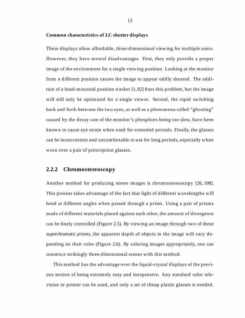
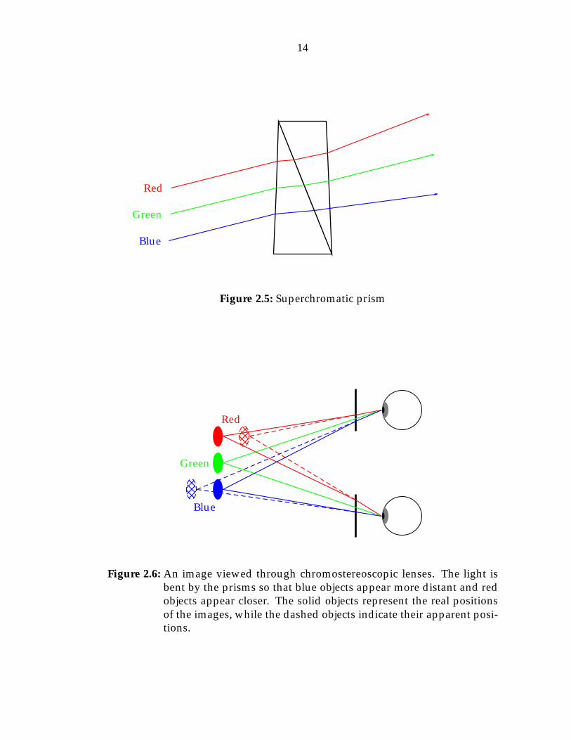
Another method for producing stereo images is chromostereoscopy [26, 108].

This process takes advantage of the fact that light of different wavelengths will

bend at different angles when passed through a prism. Using a pair of prisms

made of different materials placed against each other, the amount of divergence

can be finely controlled (Figure 2.5). By viewing an image through two of these

superchromatic prisms, the apparent depth of objects in the image will vary de-

pending on their color (Figure 2.6). By coloring images appropriately, one can

construct strikingly three-dimensional scenes with this method.

This method has the advantage over the liquid-crystal displays of the previ-

ous section of being extremely easy and inexpensive. Any standard color tele-

vision or printer can be used, and only a set of cheap plastic glasses is needed.

14

Red

Green

Blue

Figure 2.5: Superchromatic prism

Red

Green

Blue

Figure 2.6: An image viewed through chromostereoscopic lenses. The light isbent by the prisms so that blue objects appear more distant and redobjects appear closer. The solid objects represent the real positionsof the images, while the dashed objects indicate their apparent posi-tions.

15

In fact, this is actually an enhancement of an effect already present in human

vision [58,116], and images made with this technique can often be viewed with-

out the use of special lenses at all. However, it requires that the color of the

image be totally devoted to depth. This limits the technique’s usefulness for sci-

entific visualization or the display of real scenes, making it mainly appropriate

for artists.

2.2.3 Head-mounted displays

In 1968, Ivan Sutherland eliminated the free standing television completely and

mounted a pair of miniature CRTs directly over the user’s eyes [111]. Combined

with a position tracker, this provides both binocular disparity and motion paral-

lax, creating an illusion of total immersion in a three-dimensional environment.

Sutherland’s research gave birth to the field of virtual reality [17,110]. Although

only now becoming commercially viable, this technology has gained a great

deal of interest, and is likely to become the method of choice for many applica-

tions.

Nevertheless, it suffers from many of the same drawbacks as the liquid-

crystal displays described in Section 2.2.1. A head-mounted display system can

only be used by a single person at a time. Instead of the flicker and ghosting of

the LC displays, head-mounted displays currently suffer from a lag between the

time the user moves his head and the time the image updates, causing a form of

motion sickness known as “simulator sickness”. These weaknesses make head-

mounted displays unsuitable for many applications.

16

Images Barrier

Figure 2.7: A parallax barrier display with two images. The barrier ensures thatonly one image is visible from any given position. By decreasing theslit size, a display with more images can be created.

2.2.4 Autostereoscopic displays

One of the major drawbacks of all of the above systems is the need to don spe-

cial headgear to use them. A simple desk monitor that can produce a three-

dimensional image all by itself would be much more convenient. Several manu-

facturers are therefore experimenting with autostereoscopic imaging techniques.

The first such technique was the parallax barrier [54, 55], invented in 1903.

A parallax barrier is an opaque screen with many thin vertical slits, placed a

slight distance in front of a piece of photographic film (Figure 2.7). An image

projected through the barrier will be recorded on the film as a series of thin

strips. Depending on the width and separation of the slits, a number of images

can be recorded in this way from different angles without interfering with each

other. Once the film is developed, the parallax barrier will ensure that a viewer

looking at it from any given direction will see only the image taken from that

angle. This not only produces a stereoscopic effect, it also allows the user to

17

Images Lens

Figure 2.8: A lenticular sheet display with two images. The lenses bend the lightso that only one image is visible from any given position.

move around the display and view the 3D environment from any angle.

A related technique is the lenticular sheet [95], invented in the 1920’s. In-

stead of an opaque barrier, the image is covered with a transparent sheet com-

posed of a series of cylindrical or elliptical lenses (Figure 2.8). Rather than

blocking light from a given direction, these lenses redirect it so that the viewer

only sees the appropriate part of the composite image. This allows much more

light into the system, resulting in brighter, clearer images than those provided

by the parallax barrier.

Both of these methods can readily be adapted to electronic displays. A

monitor can easily be designed with a built in parallax barrier or lenticular

sheet [18, 39, 104], and software to produce the necessary composite images is

easy to write. Of course, there is a trade-off between image resolution and the

number of images, since the resolution of the underlying monitor remains fixed.

In addition, several other variations on this theme unique to electronic displays

are also possible [40, 41, 112].

18

Although they free the user from the inconvenience of headgear, these dis-

plays are still not perfect. The number of discrete angles for which views can be

provided is limited, and the changes between them are abrupt and disturbing.

This problem can be solved with the addition of a position tracker [103], but this

reintroduces the problem of headgear and prevents them from being effectively

used by more than one person.

2.2.5 Stereoblindness

In addition to the individual disadvantages possessed by all of these stereo-

scopic technologies, there is the problem of stereoblindness. A small but non-

negligible portion of the population lacks the ability to fuse stereo pairs into

a three-dimensional whole without additional depth cues [96, 99]. The exact

number of people who suffer from this is a matter of debate, and appears to be

dependent on the testing method used, but all studies place it between one and

ten percent of the population. For these people, most of the devices described

in this section are useless. In the next two sections, we will see several exper-

imental displays designed to take advantage of all of the physiological depth

cues.

2.3 Direct volume displays

Direct volume displays draw points throughout a three-dimensional volume of

space. They are also known as multi-planar displays, since they essentially have

several image planes rather than the single one provided by a two-dimensional

monitor. Because the images created are truly three-dimensional, they provide

19

Mon

itor

Viewer

Vibrating Mirror

ImageVolume

Figure 2.9: A varifocal mirror display. Due to the curvature of the mirror, theimage of the monitor moves through a large volume, despite thesmall range of the mirror itself.

all of the physiological depth cues.

2.3.1 Varifocal mirror displays

The first multi-planar displays were varifocal mirror devices [98, 106]. These

displays consisted of a rapidly oscillating mirror and an ordinary CRT moni-

tor (Figure 2.9). They were used by viewing the reflection of the monitor in

the mirror. Because the mirror was oscillating, the position of the image re-

flected in it would also oscillate. By rapidly changing the image displayed on

the monitor, one could create the illusion of a continuum of images floating in

three-dimensional space.

2.3.2 Rotating screen displays

Varifocal mirror displays were limited in both the size of their display volume

and the angles from which they could be viewed. They have since been aban-

20

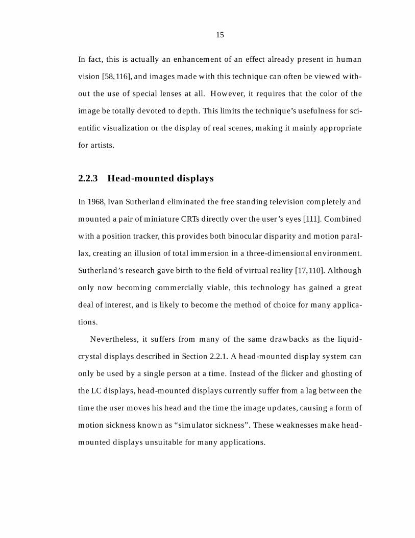
(a) Translucent screen (b) LED array

Figure 2.10: Rotating screen displays. (Images from [88, pg. 237] and [107], re-spectively.)

doned in favor of more versatile rotating screen displays [30,107,124,125]. These

use a flat or helical screen rotating within an enclosed volume (Figure 2.10). In

most cases, the screen is translucent and a laser is used to draw points on it as it

passes through space. In a few devices the screen itself is composed of an array

of LEDs which can be rapidly turned on and off. With these devices, one can

theoretically draw arbitrarily complex figures throughout the display volume.

Not only do rotating screen displays take advantage of all of the physiologi-

cal depth cues, they allow any number of people to use them, and they provide a

full 360 degree field of view. This makes them ideally suited for certain classes of

applications, such as the air traffic control system example discussed in Section

2.1. However, while they gain physiological depth cues, they lose an important

psychological cue: occlusion. In addition, their use is limited to environments

which can be contained in the display volume. This makes them unsuitable for

large environments or applications requiring realistic rendering.

21

2.4 Holographic displays

Perhaps the most promising 3D display technology is the holographic display

system. Holograms work by completely reproducing the light (at a wavelength

scale) given off by an actual object or objects. They therefore provide all the

depth cues present in the real scene, both psychological and physiological. Al-

though not yet a commercial reality, an electronic display based on holographic

principles would produce a completely realistic three-dimensional image of an

environment, viewable from any angle, without any headgear needed.

Stephen Benton [4–6] provides an overview of holographic imaging technol-

ogy prior to 1985. Since then, there has been an explosion of proposed meth-

ods for constructing a high-resolution, real-time, electronic holographic dis-

play [7,9–11,13,14]. Although it remains unclear which of these will prove to be

most viable, all but the most skeptical developers agree that commercially avail-

able electronic holographic displays will be a reality within twenty years [126].

Chapter 3

Computer-Generated Holography

The word hologram comes from the Greek roots holos and gramma and literally

means “total message”. In general, holography refers to any process which

allows both the magnitude and phase of a wave to be recorded and later re-

constructed. It can be applied to any type of wave phenomenon, including

light, sound, and quantum mechanical particle scattering. However, the most

well known forms of holograms are those made with visible light. These three-

dimensional images, which can be found on everything from toys to credit cards

to museum walls, are what we wish to simulate.

The hologram was introduced in 1948 by Dennis Gabor [42–44], who pro-

posed it as a means of improving the resolution of the electron beam micro-

scope. He exposed a piece of photographic film to monochromatic light passing

through a very small photographic slide. This light formed a microscopic inter-

ference pattern, which the film was able to capture. Gabor showed that illumi-

nating the developed film with the same light source would produce an image

of the slide, suspended in space at it’s original position. He called this process

wavefront reconstruction.

22

23

Due to the lack of a coherent light source, little progress was made in the

field until the invention of the laser in 1960. This device enabled Leith and

Upatnieks [63–65] to produce the first holograms of solid objects. Since then,

significant improvements in holographic recording techniques have been made,

and holography has become a minor art form. However, the basic principles

remain the same: coherent light is passed through or reflected off of a set of

objects, combined with a reference beam, and the resulting interference pattern

is used to expose a piece of film.

Unfortunately, while producing a hologram is not much more complicated

than producing a photograph, computing one is a far more difficult task than

computing a two-dimensional image. One can begin to understand this com-

plexity by considering the fact that a photograph contains the image seen from a

single point, while a hologram contains the images seen from every point across

it’s surface. However, the problem is even more fundamental than this. Holo-

grams and photographs require completely different models of light to com-

pute.

Traditional rendering algorithms are based on the particle model of light.

Light sources are considered emitters of photons or rays, which travel through

space in straight lines until they strike a surface, where they can partially or

completely reflect and/or refract. How closely this process is modeled varies

widely depending on the algorithm used, but in all cases, the light propagation

obeys simple rules of geometric optics. In general, under this model, the light

throughout space can be represented by a real-valued scalar function L(~x; ~!; �)

of six variables: the position ~x = (x; y; z); the direction of propagation ~! =

(�; �); and the wavelength �. Computing an image is essentially equivalent

24

to evaluating this function at a single point in space (for a pinhole camera) or

across a small region (for a finite aperture).

On the other hand, holography theory is based on the wave model of light.

Under this model, light can be represented by a complex-valued vector field

~F (~x; �) of four variables. This can be either the electric field, ~E, or the magnetic

field, ~B. The intensity of light at a given point is proportional to the square of

this field’s magnitude. Instead of following simple geometric rules, ~F propa-

gates according to a set of differential equations. To compute a hologram, we

must solve these equations to evaluate this function across it’s entire face.

From a computational standpoint, the key difference between these two rep-

resentations is their relative coherence. The function for the particle model is

dominated by low-frequency components and possesses a great deal of coher-

ence. Rendering algorithms can take advantage of this by making numerous ap-

proximations which decrease computation time without adversely affecting the

image quality. The wave model representation is dominated by high-frequency

terms on the scale of the wavelength of light. This means that the computation

must be carried out at a much finer level.

A numerical representation of a hologram requires about 109 sample points

per square centimeter. To perfectly simulate the hologram’s formation, the ob-

jects in the scene must be sampled at the same level, and the contribution of

every object point to every point on the hologram must be considered. Even

for small holograms of simple scenes, this can require over 1020 operations, well

beyond the limits of current computer technology.

Research in computer-generated holography has therefore focused on find-

ing approximations in the scene description and the light itself which allow the

25

complexity to be reduced. The early evolution of these techniques can be ob-

served in several review papers [27, 34, 52, 62, 68, 115] dating from 1971 through

1989. This chapter discusses these methods as well as more recent ones, and

examines their advantages and disadvantages.

3.1 Notation

We begin by describing the notational conventions which will be used through-

out this thesis. We use italic text to represent real-valued variables and functions

(a, f , F , x, : : : ), and bold italic for complex values (a, f , F , x, : : : ). Oblique

text is used for constants (a, f , F, x, : : : ). In particular, i is used to denotep�1.

Spatial coordinates are denoted by ~x, with or without a subscript (~xp,~xs, : : :

). For a point ~xp, the individual coordinate components are (xp; yp; zp). Vectors

are denoted by other letters, notably ~r and ~k. Given a vector ~r, its magnitude is

represented by the scalar r � k~rk and its direction by the unit vector r � ~rr. In

Cartesian coordinates, its components are written as (rx; ry; rz), while in polar

coordinates we use (r; r�; r�). We also use ~! = (�; �) to denote a generic unit

vector.

For an expression U dependent on variable x, we define

Fx fU(x)g (k) �Z +1

�1

U(x)ei2�kxdx(3.1)

to be the Fourier transform of U with respect to x evaluated at k. Similarly, the

inverse Fourier transform is given by

F�1k fu(k)g (x) �

Z +1

�1

u(k)e�i2�kxdk.(3.2)

26

Scene

b

~xs

~rns

Hologram

b

~xh

Observer

x

y

z

Figure 3.1: A sample scene to be rendered holographically

In discrete form, for an array U i with n samples, these equations become

Fi fU igj �Xi

U iei2�

ij

n(3.3)

F�1j fujgi �

Xj

uje�i2�

ij

n .(3.4)

3.2 Problem definition

For the purposes of this discussion, we will consider the task of computing a

hologram of the simple scene shown in Figure 3.1. The holographic film lies in

the x-y plane centered at the origin, and will be viewed by observers in the pos-

itive z region. The objects are shown here a short distance behind the hologram,

but in general may be placed anywhere, including in front of, or even passing

through, the hologram plane.

We assume that the scene is illuminated by monochromatic light of wave-

length � and wavenumber k = 2��

. Although the light ~F is a vector field, we

will consider only one vector component, since, in most circumstances, the three

components operate almost independently and identically. Our representation

27

for the light throughout space becomes F (~x). Note that these assumptions ig-

nore some of the finer details of electro-magnetic wave propagation, notably

near- and sub-surface effects, but these factors can be safely omitted when com-

puting a hologram. The value of F at all points ~xs on the objects’ surfaces is

directly related to the light emitted by and reflected from them. It can be found

using existing illumination algorithms in combination with a high frequency

phase factor to account for directional variations. Given this F (~xs), we must

determine the value of F (~xh) at every point on the hologram.

Note that to record a hologram, the light from the objects must be combined

with a reference wave, and to reconstruct the image, the same wave must be

used to illuminate the hologram. For the sake of simplifying this discussion,

we will omit this wave and treat the hologram as if it were made of some ideal

substance that can perfectly record, and later reproduce, both the magnitude

and phase of light across it. Nevertheless, the reader should be aware that when

implementing any of the algorithms discussed here, it will be necessary to add

such a reference wave to the computed field F (~xh) in order to produce a usable

hologram.

For simplicity, we assume that the hologram is square, with sides of length

D, and that the same sample spacing, �, is used in both directions. If we define

� to be the largest angle at which the hologram will be viewed (Figure 3.2), then

� is constrained by

� ��

4 sin�.

We use twice the usual Nyquist sampling rate here because the holographic

recording process captures the complex wavefront as a real-valued intensity

field, so more samples are needed to reconstruct both the real and imaginary

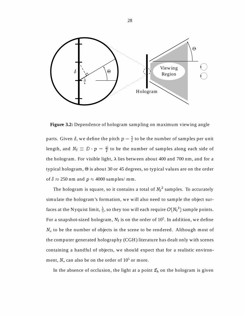
28

Hologram

ViewingRegion

�

�

�4

�

Figure 3.2: Dependence of hologram sampling on maximum viewing angle

parts. Given �, we define the pitch p � 1

�to be the number of samples per unit

length, and N� � D � p = D

�to be the number of samples along each side of

the hologram. For visible light, � lies between about 400 and 700 nm, and for a

typical hologram, � is about 30 or 45 degrees, so typical values are on the order

of � � 250 nm and p � 4000 samples/mm.

The hologram is square, so it contains a total of N�2 samples. To accurately

simulate the hologram’s formation, we will also need to sample the object sur-

faces at the Nyquist limit, �2, so they too will each require O(N�

2) sample points.

For a snapshot-sized hologram, N� is on the order of 105. In addition, we define

No to be the number of objects in the scene to be rendered. Although most of

the computer generated holography (CGH) literature has dealt only with scenes

containing a handful of objects, we should expect that for a realistic environ-

ment, No can also be on the order of 105 or more.

In the absence of occlusion, the light at a point ~xh on the hologram is given

29

by

F (~xh) =1

i�

ZZF (~xs)

eikr

r(ns � r)d~xs,(3.5)

where F (~xh) is the light at location ~x, ~xs is a position on an object surface, ~xh is

a position on the hologram, ~r is the vector from ~xs to ~xh, and ~ns is the surface

normal at ~xs (see Goodman [45, Ch. 3-4] for details). For a single object, this in-

tegral can be computed numerically with O(N�2) operations. The computation

must be performed for all No objects and all N�2 hologram points, so the total

time required is O(NoN�4).

When objects are allowed to occlude one another, as is the case for all but

the most trivial scenes, accurate simulation of the hologram formation requires

accounting for the diffraction around objects. This is an extremely difficult prob-

lem to solve for arbitrary environments, so we usually assume that diffraction

has a negligible effect on the image seen by the viewer, and consider only direct

point-to-point occlusion. Equation (3.5) becomes

F (~xh) =1

i�

ZZV (~xs; ~xh)F (~xs)

eikr

r(ns � r)d~xs,(3.6)

where V (~xs; ~xh) is 1 if ~xs and ~xh are directly visible from one another, and 0

if another object lies between them. This visibility function requires, at worst,

O(No) time to compute, so the total time to compute the hologram becomes

O(No2N�

4). Since No and N� can both number in the hundreds of thousands, it

is necessary to find ways to reduce this complexity for the problem to become

feasible.

30

bbbbbbbbbbbbbbbbbbbbb

bbbbbbbbbbbbbbbbbbbbb

bbbbbbbbbbbbbbbbbbbbb

bbbbbbbbbbbbbbbbbbbbb

b

b

b

b

b

b

b

b

b

b

b

b

b

b

b

b

b

b

b

b

b

b

b

b

bbbbbb

bbbbbb

bbbbbb

bbbbbb

bbbbbbbbb

bbbbbbbbb

bbbbbbbbb

bbbbbbbbb

b

b

b

b

b

b

b

b

b

b

b

b

b

b

b

b

b

b

b

b

b

b

b

b

b

b

b

b

b

b

b

b

b

b

b

b

b

b

b

b

b

b

b

b

bbbbbbbbb

bbbbbbbbb

bbbbbbbbb

bbbbbbbbb

bbbbb

bbbbb

bbbbbb

bbbb

b

b

b

b

b

b

b

b

b

b

Hologram

Figure 3.3: Scene with objects replaced by point sources

3.3 Geometric simplifications

One way in which the complexity can be reduced is to simplify the geome-

try of the scene to forms whose emissions can be more easily computed. Wa-

ters [118, 119] replaced the objects with a series of closely spaced point sources

lining the surface edges (Figure 3.3). This reduces the dimensionality of the ob-

jects from two-dimensional surfaces to one-dimensional lines, allowing a corre-

sponding reduction in the number of object sample points required. Addition-

ally, since we are no longer trying to display realistic surfaces, we no longer need

to sample the objects at wavelength scale. It is sufficient to position the points

closely enough so that the gaps are not visible to an observer. The complexity

of the algorithm becomes O(NoN�2Np), where Np is the number of point sources

per object, which can now be measured in hundreds rather than hundreds of

thousands.

Frere and Leseberg [24,67] took this a step further by finding analytical solu-

tions for the propagation of light from a luminous line segment to the hologram

31

Hologram

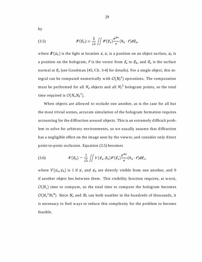
Figure 3.4: Scene with objects replaced by line sources

(Figure 3.4). This allows the objects to be represented by a few lines, rather than

hundreds of points. The time required now becomes O(NoN�2Nl).

Despite the increased speed of this algorithm, a great deal is lost by replacing

the objects with points or lines. Obviously, we cannot present objects with realis-

tic surface properties, such as textures and complex reflection patterns, because

there are no surfaces at all. Additionally, lines cannot provide any occlusion, so

objects which should be hidden behind others will instead be visible through

them, turning large scenes into confusing jumbles. Thus, while this technique is

suitable for applications where we might use a wire-mesh rendering program,

such as some engineering and design problems, it will not produce realistic im-

ages.

3.4 Fourier holography

Both in research and in practice, the most widely used CGH methods are forms

of Fourier holography. This subfield uses a variety of approximations to ex-

32

xs

ys

xh

yh

Hologram

R

Figure 3.5: A Fraunhofer hologram. The scene consists of a single planar objectplaced a large distance from the film plane.

press the light received by the hologram in terms of a Fourier transform of the

light emitted by the objects. Such representations allow the computation to be

performed using fast Fourier transforms (FFTs) [19, 20, 81], greatly reducing the

time required.

3.4.1 Fraunhofer holograms

The very first computer-generated holograms were Fraunhofer holograms [21].

Fraunhofer holograms are made by placing the object(s) a very great distance

from the holographic film. Specifically, suppose our scene consists of a single

planar object lying perpendicular to the z axis, as shown in Figure 3.5. Then

the Fraunhofer approximation [45, Ch. 4] requires that the distance R between

it and the hologram is large enough that

R�� maxs(x

2s + y2s)

4�.(3.7)

At this distance, the difference in path length between a point on the hologram

and any two points on the object will be significantly less than the wavelength.

33

This is quite large, so Fraunhofer holograms are not actually made with objects

at that distance. Instead, the object is placed much closer, and lenses are used to

optically move the object far enough away.

This approximation allows several simplifications to be made to Equation

(3.5). The magnitude of ~r is dominated by R, and can be approximated by the

first few terms of a binomial expansion:

r � R

"1 +

1

2

�xh � xsR

�2+

1

2

�yh � ysR

�2#.(3.8)

Combining Equations (3.5), (3.7), and (3.8) yields

F (xh; yh) =eikR

i�Rei

k2R

(x2h+y2

h)

ZZF (xs; ys) e

�i2�R�

(xhxs+yhys)dxsdys(3.9)

=eikR

i�Rei

k2R

(x2h+y2

h)F�1(xs;ys)

fF (xs; ys)g�xh

R�;yh

R�

�.(3.10)

Equation (3.10) is just the inverse Fourier transform of F , evaluated at�xhR�; yhR�

�, and multiplied by a quadratic phase factor. It should therefore come as

no surprise that this technique was first used to compute holograms the year af-

ter the introduction of the fast Fourier transform [33]. Using FFTs, this equation

can be computed in O(N�2 logN�) time. If we add a factor of No to this com-

plexity, we can make holograms of multiple planar objects at different depths.

Because of their speed and simplicity, much of the early work in computer-

generated holography was done with this type of hologram [21–23, 60, 61, 82].

However, while Fraunhofer holograms are useful for a number of applications,

such as developing pattern recognition systems, they have several drawbacks

which make them unsuitable for use in three-dimensional imaging systems.

The source of many of these problems is the large distanceR between the ob-

jects and the hologram. For example, if our hologram and objects are a few cen-

timeters across, Equation (3.7) requires that R be over two kilometers. Lenses

34

are used in the reconstruction process to allow the image to be seen despite this

great distance, but the three-dimensionality of the objects is entirely lost. There

will be no parallax, perspective, or depth of focus effects, because the light rays

reaching the eye are almost perfectly parallel. For this reason, creating Fraun-

hofer holograms with multiple depth planes is not useful, since the difference

in depth will not be apparent to a viewer.

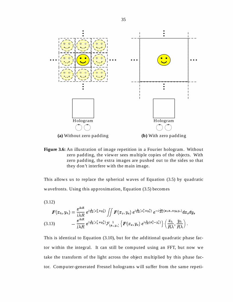
Another problem is that the fast Fourier Transform can only approximate its

continuous counterpart. In particular, it is cyclical in nature. The integral in

Equation (3.10) has infinite extent, but the transform can only be applied over a

finite region. The FFT operates with the assumption that the contents of this re-

gion repeat endlessly across the plane. This means that a Fourier hologram will

display not just the desired image, but an infinite series of duplicates stretching

out to the sides (Figure 3.6). To prevent these extra images from interfering with

the appearance of the hologram, we need to extend the limits of the sampling

array representing the object by adding zeroes around the edges, so as to make

it large enough that the duplicates are moved out of view. This can significantly

increase the computation time.

3.4.2 Fresnel holograms

The problems associated with the large distance between the objects and the

hologram were greatly alleviated by moving to the Fresnel regime. The Fresnel

approximation [45, Ch. 4] assumes that

R3 ��

4�maxs;h

h(xh � xs)2 + (yh � ys)2

i2.(3.11)

35

b

b

b

b

b

b

b b bbbb

Hologram

(a) Without zero padding

b

b

b

b

b

b

b b bbbb

Hologram

(b) With zero padding

Figure 3.6: An illustration of image repetition in a Fourier hologram. Withoutzero padding, the viewer sees multiple copies of the objects. Withzero padding, the extra images are pushed out to the sides so thatthey don’t interfere with the main image.

This allows us to replace the spherical waves of Equation (3.5) by quadratic

wavefronts. Using this approximation, Equation (3.5) becomes

F (xh; yh) =eikR

i�Rei

k2R

(x2h+y2

h)

ZZF (xs; ys) e

ik2R

(x2s+y2s ) e�i

2�R�

(xhxs+yhys)dxsdys

(3.12)

=eikR

i�Rei

k2R

(x2h+y2

h)F�1

(xs;ys)

nF (xs; ys) e

ik2R

(x2s+y2s )o� xh

R�;yh

R�

�.(3.13)

This is identical to Equation (3.10), but for the additional quadratic phase fac-

tor within the integral. It can still be computed using an FFT, but now we

take the transform of the light across the object multiplied by this phase fac-

tor. Computer-generated Fresnel holograms will suffer from the same repeti-

36

z

y

(a) Objects (b) Depth planes (c) Projection

Figure 3.7: A Fresnel hologram using multiple planar objects to simulate athree-dimensional scene. The objects are projected onto the near-est depth plane, and the hologram is computed by adding the holo-grams that would be produced by each of these planes individually.

tion problems as Fraunhofer holograms, requiring zero-padding, but the depth

problems are greatly reduced.

For a typical hologram, Equation (3.11) requires thatR be at least five meters.

This is quite large, but is significantly less than the two kilometers needed for

the Fraunhofer holograms. Lenses will still be necessary in the reconstruction

process, but now a limited amount of depth effect will be visible. This allows

holograms with several objects at different depths to be created by adding the

results of multiple applications of Equation (3.13) [72, 120, 121].

This process introduces a new problem: how to produce holograms of arbi-

trary three-dimensional scenes using an algorithm meant only for two-dimen-

sional objects lying parallel to the hologram plane. Two issues are involved:

computing holograms of objects which are not parallel to the hologram; and

computing holograms where near objects occlude farther ones.

The first method [73] used to handle non-parallel objects is illustrated in

Figure 3.7. The scene is divided into several slices at different depths. Within

each of these slices, the object surfaces are orthographically projected onto a

37

single plane. Equation (3.13) is then applied to each of these planes, and the

results are summed to get the complete hologram.

This technique works well provided a sufficient number of slices are used so

that the discrete depths appear continuous. If only a few depth planes are used,

then the viewer will be able to see the individual slices, and the objects will

not appear realistic. However, the time required, O(NRNoN�2 logN�), is linearly

dependent on the number of planes, NR, so a hologram with a large number of

planes will be computationally expensive.

This problem was solved when Leseberg and Frere [71] showed how Equa-

tion (3.13) could be modified to handle arbitrarily inclined planar objects. In

addition to the FFT, an interpolation step is used to transform the light from the

space of the inclined plane to hologram space. The extra step does not increase

the computational complexity. We can now compute a hologram of any scene

that can be represented solely by a set of polygons, using only one FFT and in-

terpolation operation per polygon, so the complexity is now reduced back to

O(NoN�2 logN�).

Both the multiplane and tilted plane techniques deal with multiple surfaces

by adding the holograms each would individually produce. This prevents con-

sideration of any occlusion that would normally be present, allowing far objects

which should be blocked out by near ones to instead be visible through them.

Ichioka et al. [53] showed how the first of these methods could be modified,

without increasing the computational complexity, to cause the depth-planes to

occlude those behind them. The technique can theoretically be applied to the

algorithm used by Leseberg and Frere, but would require a series of repeated

interpolation steps which would seriously degrade the final image. Thus, we

38

cannot get occlusion without the increased cost of the depth-plane method.

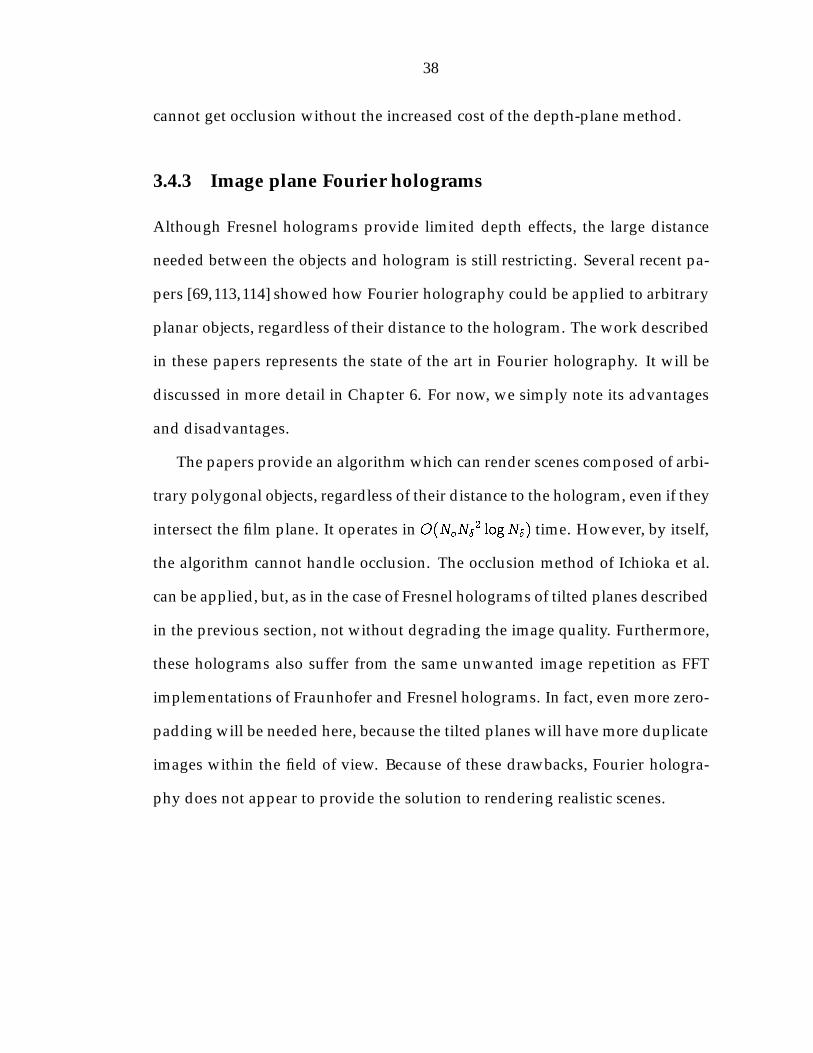
3.4.3 Image plane Fourier holograms

Although Fresnel holograms provide limited depth effects, the large distance

needed between the objects and hologram is still restricting. Several recent pa-

pers [69,113,114] showed how Fourier holography could be applied to arbitrary

planar objects, regardless of their distance to the hologram. The work described

in these papers represents the state of the art in Fourier holography. It will be

discussed in more detail in Chapter 6. For now, we simply note its advantages

and disadvantages.

The papers provide an algorithm which can render scenes composed of arbi-

trary polygonal objects, regardless of their distance to the hologram, even if they

intersect the film plane. It operates in O(NoN�2 logN�) time. However, by itself,

the algorithm cannot handle occlusion. The occlusion method of Ichioka et al.

can be applied, but, as in the case of Fresnel holograms of tilted planes described

in the previous section, not without degrading the image quality. Furthermore,

these holograms also suffer from the same unwanted image repetition as FFT

implementations of Fraunhofer and Fresnel holograms. In fact, even more zero-

padding will be needed here, because the tilted planes will have more duplicate

images within the field of view. Because of these drawbacks, Fourier hologra-

phy does not appear to provide the solution to rendering realistic scenes.

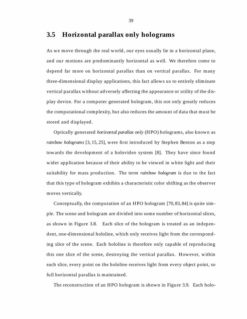
39

3.5 Horizontal parallax only holograms

As we move through the real world, our eyes usually lie in a horizontal plane,

and our motions are predominantly horizontal as well. We therefore come to

depend far more on horizontal parallax than on vertical parallax. For many

three-dimensional display applications, this fact allows us to entirely eliminate

vertical parallax without adversely affecting the appearance or utility of the dis-

play device. For a computer generated hologram, this not only greatly reduces

the computational complexity, but also reduces the amount of data that must be

stored and displayed.

Optically generated horizontal parallax only (HPO) holograms, also known as

rainbow holograms [3, 15, 25], were first introduced by Stephen Benton as a step

towards the development of a holovideo system [8]. They have since found

wider application because of their ability to be viewed in white light and their

suitability for mass production. The term rainbow hologram is due to the fact

that this type of hologram exhibits a characteristic color shifting as the observer

moves vertically.

Conceptually, the computation of an HPO hologram [70, 83, 84] is quite sim-

ple. The scene and hologram are divided into some number of horizontal slices,

as shown in Figure 3.8. Each slice of the hologram is treated as an indepen-

dent, one-dimensional hololine, which only receives light from the correspond-

ing slice of the scene. Each hololine is therefore only capable of reproducing

this one slice of the scene, destroying the vertical parallax. However, within

each slice, every point on the hololine receives light from every object point, so

full horizontal parallax is maintained.

The reconstruction of an HPO hologram is shown in Figure 3.9. Each holo-

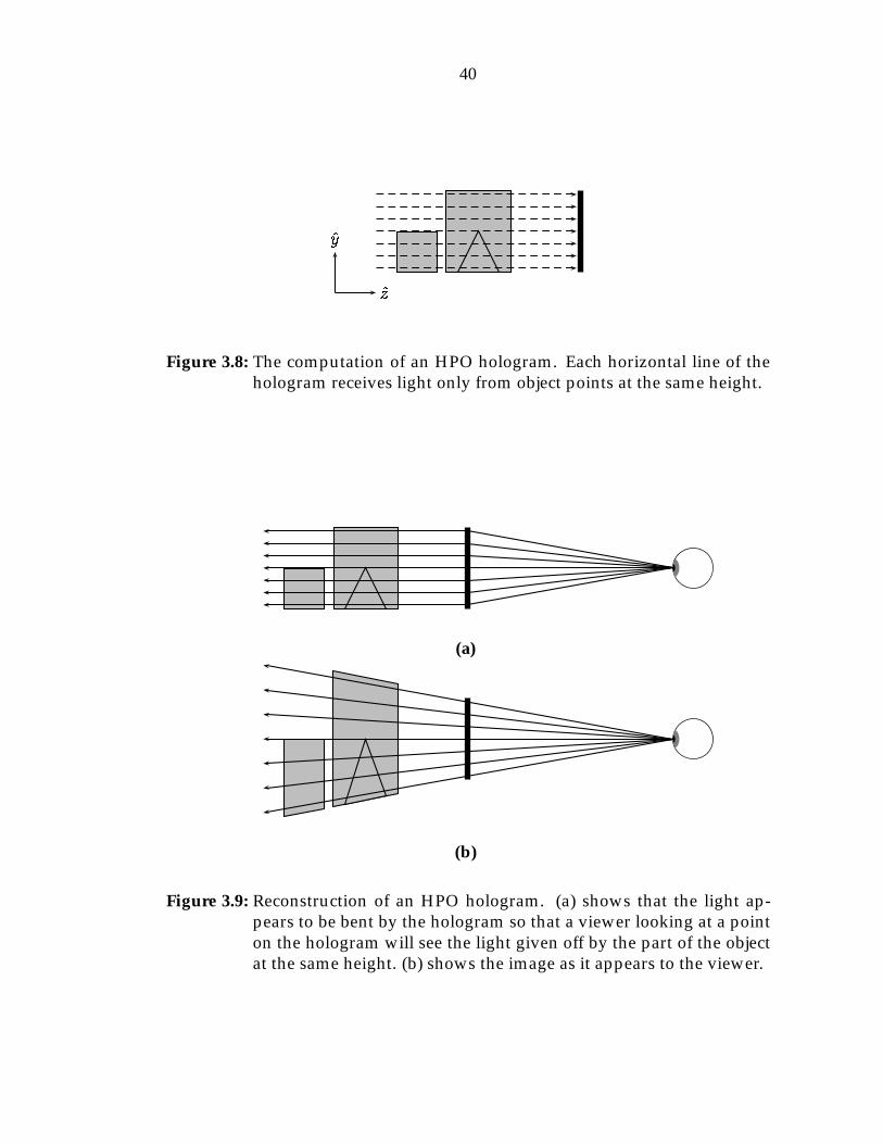
40

z

y

Figure 3.8: The computation of an HPO hologram. Each horizontal line of thehologram receives light only from object points at the same height.

(a)

(b)

Figure 3.9: Reconstruction of an HPO hologram. (a) shows that the light ap-pears to be bent by the hologram so that a viewer looking at a pointon the hologram will see the light given off by the part of the objectat the same height. (b) shows the image as it appears to the viewer.

41

line produces an image of the corresponding slice of the hologram, which it

projects uniformly in all directions. Thus no matter what the height at which

the user is positioned, the entire hologram will be visible, although the image

will be shifted and distorted depending on this position. This distortion is exag-

gerated here for the purposes of illustration. It is normally not as pronounced,

and does not interfere with the appearance of the hologram.

Because the vertical parallax has been eliminated, it is no longer necessary

to sample the hologram at near wavelength scale in the vertical direction. A

resolution on the order of that of an ordinary CRT display is satisfactory. We

define � to be the new vertical spacing, and note that it is several orders of

magnitude larger than �. The number of vertical samples becomes N� � D

�.

Modifying equation Equation (3.6) to integrate only in the horizontal direction,

we find that the hologram can be computed in O(No2N�N�

2) time, significantly

less than the O(No2N�

4) required for full parallax. In addition, the use of HPO

holograms can be combined with other techniques, such as Fourier holography

[66], to reduce the complexity even further.

This method is not without its drawbacks. First of all, there is the obvious

fact that the holograms lack vertical parallax, as well as the slight image distor-

tion mentioned above. A second and more subtle problem is the fact that HPO

holograms cannot focus light vertically. This produces an astigmatism effect

which increases with the object depth. The human visual system can only toler-

ate a certain amount of astigmatism, so the usable depth of an HPO hologram at

which fine focus can be achieved will be limited [85, pg. 26]. Nevertheless, HPO

holograms are perfectly suitable for a wide range of applications, and because of

their relative computation speed and lower data size, the first few generations

42

of commercial holographic displays are likely to use this technique.

3.6 Holographic stereograms

First developed as a means of producing holograms of large, naturally illumi-

nated scenes, holographic stereograms [89] provide a simple and computation-

ally inexpensive means of producing computer generated holograms. Figure

3.10 shows a simplified overview of the optical generation of a holographic

stereogram. The apparatus and geometric layout for this process can vary wide-

ly, but the general principles remain the same. A series of photographs are

taken of the scene by a camera moving along a guide rail. The photographs are

then projected, using a coherent light source, onto a translucent screen one at

a time, and each one is used as the object to produce a thin strip of the holo-

gram. Someone looking through the nth strip will see an image of the photo-

graph taken at the nth position. Thus, someone looking at the hologram as a

whole will see a series of images, each taken from a slightly different position,

which will combine to produce an illusion of three-dimensionality. The effect is

similar to that of the lenticular screen stereograms described in Chapter 2, but

holographic stereograms can provide views from many more discrete positions.

This method can easily be adapted to computationally modeled scenes by

substituting computer generated images for the photographs [48, 57]. Any suit-

able computer graphics software can be used to render the images. They can

then be transferred to film, and combined in a hologram using the same ap-

paratus as before. The hardware can be eliminated by computing the hologram

strips directly from the rendered images using FFTs or other algorithms [90,128].

43

n� 1 n n+ 1

x

z

(a) Recording of images

n� 1 n n+ 1

(b) Image set

n� 1 n n+ 1

projector

screen

barrier

hologram

(c) Construction of hologram

Figure 3.10: Creation of a holographic stereogram. A series of photographs aretaken of the scene. These photographs are then projected onto ascreen, and a thin hologram is made of each of the images.

44

There is a sharp contrast between this method and those described in the

preceding sections. In Sections 3.3 and 3.4, approximations were made in the

structure of the objects, but we still attempted to accurately simulate the prop-

agation and interference of light which produces the hologram. In Section 3.5,

we subdivide the world into some number of independent slices, but within

each slice we again still try to accurately simulate the interference. In the holo-

graphic stereogram, on the other hand, we are less concerned with the process

that forms the hologram than we are with it’s appearance to an observer. Re-

calling the discussion about particle vs. wave models at the beginning of this

chapter, we see that the holographic stereogram method performs part of the

computation (i.e. generating the images) using the particle model, and then

switches to the wave model to produce the hologram. As was noted, compu-

tation can be done far more efficiently with the particle model than the wave

model. This accounts for the great increase in speed offered by the stereogram.

3.7 Diffraction specific computation

In this section, we will discuss a particular holographic stereogram algorithm

called diffraction specific computation, developed by Mark Lucente [85–87]. The

name refers to the fact that the focus is on how the light is diffracted by the

hologram, in contrast to interference based computation, which focuses on the in-

terference phenomena which forms the hologram. Lucente described an effi-

cient method for computing holographic stereograms and showed how existing

graphics hardware could be adapted to aid in the computation process. In ad-

dition, his method also provides some simple data compression. In discussing

45

this work, we will take a different approach than that used by Lucente, describ-

ing it in somewhat more general terms and defining our own notation, in order

to more easily build upon it in the following chapters.

3.7.1 Lumigraph

We begin by taking a brief look at two papers on two-dimensional rendering.

These papers, one by Levoy and Hanrahan [74] and the other by Gortler et

al. [46], appeared at the same time and describe very similar algorithms. These

algorithms belong to a class known as image-based rendering, which uses pho-

tographs or pre-computed images from a finite number of positions to generate

views from any desired position.

A camera plane and a focal plane are defined in space, as shown in Fig-

ure 3.11. Levoy and Hanrahan parameterized these planes by (s; t) and (u; v),

respectively. Gortler et al. used the reverse of this notation. We will choose

to parameterize the camera plane by (s; t) and the focal plane by (U; V ). The

reason for this decision will become clear in Chapter 5. Any ray from the cam-

era plane that passes through the focal plane can be represented by the pair of

points at which it intersects the two planes. Therefore, these coordinate pairs

can be used to parameterize the light passing through the camera plane in any

forward direction, defining a function L(s; t; U; V ). By discretizing this domain,

we can store information about the light as a four-dimensional array. Levoy and

Hanrahan referred to this construction as a light field, while Gortler et al. called

it a lumigraph. We prefer the latter term because it emphasizes it’s relation to a

hologram.

The two papers describe methods for computing the lumigraph directly or

46

Figure 3.11: A light field / lumigraph. (figure taken from [74])

producing it by resampling photographic data. Once this array has been fully

computed, it can be used to interpolate the view seen from an point in free

space behind the camera plane. The quality of the images obtained will depend

on how finely the 4D space is sampled.

This ability to render a scene from an arbitrary position without reference to

the scene itself is very similar to what a hologram provides. In fact, a lumigraph

contains all the information that we desire from a hologram. This is not to say

that it comes close to the information content of a real hologram of the scene.

The methods used to compute a lumigraph do not even begin to approximate

the complex light propagation that produces a hologram. However, our real

concern is not with producing physically accurate simulations of the underlying

physical phenomena so much as with producing perceptually correct images.

From this standpoint, the lumigraph provides a sufficient representation of the

light, while being far easier to compute and compress. All that is needed is a

way to convert this construct to a holographic interference pattern.

47

3.7.2 Hogel representation

This is, in essence, what Lucente [85] provides: a means for converting a lumi-

graph into a hologram. It should be noted that this work predates the light field

and lumigraph papers, but we will discuss it in terms of these papers because

they provide a more familiar framework for members of the computer graph-

ics community. Before we discuss how his algorithm works, we need to define

some symbols and terminology.

We begin by noting that while traditional 2D rendering algorithms compute

the intensity of light, holograms are computed in terms of the magnitude of the

electromagnetic field, which is proportional to the square root of the intensity.

Therefore, from this point on, whenever we discuss a lumigraph L, we will

actually be referring to the square root of the quantities calculated in the light

field and lumigraph papers.

The two-plane parameterization used in the light field and lumigraph pa-

pers was chosen because it allowed efficient resampling to render new views.

However, it is less well suited to our needs. Instead, we will parameterize the

light as L(s; t; �; �), where ~s = (s; t) is the position on the camera plane and

~! = (�; �) is the direction of the incoming light. We will derive a correspon-

dence between the directional variation of L at a given point (s; t) on the camera

plane and the value of F in the neighborhood of the point (xh; yh) = (s; t) on

the hologram.

We discretize the camera plane using a regular grid with sample spacing d,

and similarly divide the hologram into square regions of this size. Recall that

in Section 3.2, we defined the size of the hologram to be D, and the sample

spacing to be �. The new distance d will be small compared to D, but still quite

48

D d �

Figure 3.12: A hogel consists of many sample points but is still much smallerthan the hologram

large compared to � (Figure 3.12). Lucente referred to these subsections of the

hologram as hogels, for “holographic elements”.

We define n� � d

�to be the one-dimensional number of samples per hogel

and Nd � D

dto be the number of hogels along one dimension of the hologram.

Note that N� = Nd�n� . Since the hogels are two-dimensional, there are n�2 total

samples per hogel and Nd2 hogels in the hologram.

In addition, we assume that we have some discretization of ~! which pro-

vides roughly uniform angular sample spacing of #. Each sample covers a solid

angle of approximately � sin2 #2, so if the viewing frustum has half-angle �,

and assuming # is small enough that sin(#) � #, then there are n# � 2�(1 �

cos�)=(�4#2) = 8(1�cos �)

#2sample directions. The total number of samples in the

lumigraph is therefore N# = Nd2n# = 8D2(1�cos �)

d2#2.

Lucente provides upper bounds on these resolutions based on the limits of

the human visual system. Let R be the distance from which a hologram will

49

d

#hvs

R

(a)

#dhvs

R

(b)

Figure 3.13: The usable resolution of a hogel representation is limited by prop-erties of the human visual system: (a) the angular resolution of theeye; (b) the size of the pupil.

typically be viewed, and let #hvs and dhvs be the angular resolution and pupil

width of the human eye, as shown in Figure 3.13. Then a spatial sampling less

than d & R#hvs will produce features too small to be discernible, while an an-

gular sampling smaller than # & dhvs

R, will be blurred out by the eye’s aperture.

At this sampling rate, the total number of samples becomes N# .8D2(1�cos�)

d2

hvs#2hvs

.

Average values for dhvs and #hvs are approximately 3mm and 10 respectively,

and typical values for R and � would be about 0:5m and 45�. This yields

d & 0:1mm and # & 200. The number of samples required for a one square

centimeter lumigraph would be N# . 3 � 108. This is already about one tenth

of the number of samples required for a hologram with the same frustum. Of

course, this is merely an upper bound. In general, it is possible to use signifi-

cantly larger sample spacing, and correspondingly fewer samples, without per-

ceptibly affecting the quality of the resulting images.

50

3.7.3 Conversion to an interference pattern

Lucente’s research dealt primarily with horizontal parallax only holograms. Al-

though his algorithms are equally applicable to the full parallax case, as will

be discussed later, this restriction happens to be useful for the purposes of an

introductory discussion. For the remainder of this chapter, we will consider the

task of converting a one-dimensional lumigraph to a hololine. We restrict our

attention to a fixed point s in the lumigraph L(�; s) and the corresponding hogel

in the hologram F (xh), which lies in the range s � d

2� xh � s + d

2. For sim-

plicity, we shift our frame of reference so that s = 0, and use L(�) to indicate

the directional variation of the lumigraph at this point. Our goal is to find a

transform T which generates an interference pattern across this region whose

emission matches the desired lumigraph:

F (xh) = T� fL(�)g (xh) .(3.14)

To develop this transform, we consider the inverse problem. Suppose we are

given a field F (xh) which is non-zero only in the range �d

2� xh � +d

2. Then

the light received by an observer at some point ~xp in space is

F (~xp) =1

i�

ZF (xh)

ei2�r�

r(z � r) dxh,(3.15)

where ~r is the vector from ~xh to ~xp (Figure 3.14(a)).

We know that the distance from which the hologram will be viewed is large

compared to the hogel size, so we can represent ~xp by a distance R and direc-

tion � from the center of the hogel (Figure 3.14(b)), and, using approximations

similar to those in Section 3.4, Equation (3.15) becomes

F (~xp) =ei2�

R�

R

cos �

i�

ZF (xh) e

�i2�xh sin �

� dxh,(3.16)

51

b

~xp

z

x

(a) Near field

hogel

b

~xp

�

R

(b) Far field

Figure 3.14: To determine the light near the hogel, the contribution from ev-ery point must be summed. At larger distances, the hogel can betreated as a point source with a directionally non-uniform emissionpattern.

This equation can be separated into independent functions of R and �:

F (~xp) = FR(R)F �(�)

F R(R) =ei2�

R�

R

F �(�) =cos �

i�

ZF (xh) e

�i2�xh sin �

� dxh

(3.17)

The R component is simply the function for a point light source, so, to an ob-

server at a large enough distance, the hogel acts like a point source with a di-

rectionally non-uniform emission, which is exactly the behavior we expect from

a point on a lumigraph. Therefore, the � part of Equation (3.17) corresponds to

L(�).

We can now define

L(�) = T �1xh

fF (xh)g (�) �cos �

i�

ZF (xh) e

�i2�xh sin �

� dxh.(3.18)

Note that the quantity L above is complex-valued, while a lumigraph L is only

real-valued. In order to convert a lumigraph to an interference pattern, we will

52

+2��

�2��

��

+�

bk

�

Figure 3.15: There is a direct correspondence between the frequency space de-composition of the light across the hogel and its far-field directionalemission. For a given point in frequency space, the correspondingdirection vector can be found by mapping the point onto the baseof a hemicircle and projecting onto the circle.

need to first transform it into a complex function by multiplying by a phase

factor, so that kLk = L. This phase factor can be chosen randomly, or it can be

used to add additional constraints which make the interference pattern better

behaved [85].

A closer examination of Equation (3.18) reveals that the integral part is an

inverse Fourier transform of F evaluated at sin ��

:

T �1xh

fF (xh)g (�) =cos �

i�F�1xhfF (xh)g

sin �

�

!.(3.19)

This indicates that there is a direct correlation between the directional variation

of light emitted by the hogel and its representation in frequency space. This is

illustrated in Figure 3.15. If we map the spatial frequency domain �2��� k �

+2��

to points along the diameter of a hemicircle, and the directional domain

�� � � � +� to angles from its center, then we can convert from one domain to

the other by projecting orthographically.

53

Now, suppose that we have sampled the hogel at n� points, xi = i � �, to

obtain an array F i = F (xi), and that we wish to obtain the value of L at some

set of discrete angles �j . The integral in Equation (3.18) becomes a summation

Lj = L(�j) =� cos �ji�

Xi

F i e�i2�

xi sin �j� .(3.20)

Since Equation (3.18) can be written as an inverse Fourier transform, we should

be able to compute Equation (3.20) as a discrete Fourier transform as long as we

choose the sample points so that the summation matches that in the definition

of the inverse DFT (Equation (3.4)). That is,

Lj =� cos �ji�

F�1i fF igj =

� cos �ji�

Xi

F ie�i2�

ijn� .(3.21)

Combining Equations (3.20) and (3.21) we have

xi sin �j�

=ij

n�

i� sin �j�

=ij

n�

�j = arcsin

j�

�n�

!= arcsin

j�

d

!.

(3.22)

Using this sampling for �, we now have an expression for the inverse of T

in terms of the inverse Fourier transform. We can invert it to obtain the desired

transform

Tj fLjgi =i�

�Fj

(Lj

cos �j

)i

,(3.23)

which can be computed with an FFT. Note that for jjj > d

�, �j is undefined. We

define the function values at these sample points to be zero.

3.7.4 Hogel basis functions

Instead of computing F from L via a direct application of Equation (3.23), Lu-

cente proposed an alternative method. He defined a set of piecewise constant

54

Figure 3.16: Lucente’s basis functions with n� = 8. Frequency space is dividedinto equal portions, each corresponding to a set of incoming direc-tions which can be found by projecting onto the unit hemicircle (asshown on the left). Each basis function has a value of 1 over one ofthese regions and 0 elsewhere (as shown on the right).

basis functions, which we will call �m(�), over the directional hemicircle, as il-

lustrated in Figure 3.16. These functions are defined by uniformly dividing fre-

quency space into n� regions and projecting them onto the hemicircle. Each

function �m(�) has a value of one over the mth region and zero elsewhere. Using

this basis, a lumigraph can be represented by a vector of coefficients [cm], such

that L(�) �Pcm�m(�). Lucente referred to [cm] as a hogel vector.

For each of these basis functions, we can compute a corresponding interfer-

ence pattern �m(x) = T� f�m(�)g (x). Lucente called these basis fringes. This can

be done as a pre-process, and the results can then be placed in permanent stor-

age. Given a hogel vector corresponding to some L, we can now compute the

55

interference pattern as the weighted sum

F i =X

cm�m;i.(3.24)

This method provides several advantages over computation via FFT. First,

as noted earlier, L(�) can be accurately represented with far fewer samples than

F (x). However, evaluating Equation (3.23) with an FFT requires the same num-

ber of samples for both Lj and F i, forcing us to do extra work in computing the

lumigraph, which can be avoided with Lucente’s method.

Second, computation with Equation (3.23) requires O(n� logn�) time, while

Equation (3.24) requires O(n�n�). For n� . logn� , F i can be computed more

rapidly by summation than FFT. By taking advantage of existing specialized

hardware, such as an accumulation buffer [31,47,122], the savings become even

greater.

Finally, the hogel vector provides a much more compact representation than

the sampled interference pattern. By decreasing n�, we can compress the data

as much as desired, albeit at the cost of accuracy.

Using this algorithm, Lucente was able to produce small, HPO holograms

in near real-time. In the following chapters, we will build on this, extending it

to full parallax, improving the compression characteristics, and decreasing the

computation time.

Chapter 4

Representation and Compression

In the previous chapter, we derived equations to convert between a point in

a one-dimensional lumigraph and a holographic line segment. To handle the

more general case of full-parallax holograms, we must extend these equations

to 2D. The lumigraph at a single point now becomes L(�; �), and the interfer-

ence pattern across the corresponding region of the hologram is F (x; y). These

functions are sampled at spatial and directional points:

~x~{ � (i1 � �; i2 � �)

~!~| � (�~|; �~|)

� arcsin

k~|k

�

d

!; arctan

j2j1

!!(4.1)

The transforms become

F~{ = T~| fL~|g~{ �i�

�F~|

(L~|

cos �~|

)~{

(4.2)

L~| = T �1~{ fF~{g~| �

� cos �~|i�

F�1~{ fF~{g~|(4.3)

With the added sampling dimension introduced by moving to the full par-

allax case, efficient compression becomes even more important. In this chapter,

56

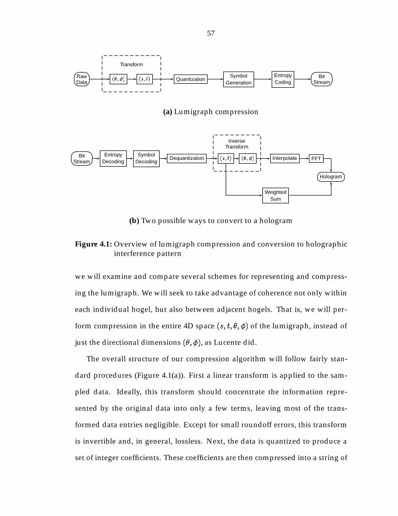
57

RawData

Transform

(�; �) (s; t) QuantizationSymbol

GenerationEntropyCoding

BitStream

(a) Lumigraph compression

BitStream

EntropyDecoding

SymbolDecoding

Dequantization (s; t) (�; �)

InverseTransform

Interpolate FFT

WeightedSum

Hologram

(b) Two possible ways to convert to a hologram

Figure 4.1: Overview of lumigraph compression and conversion to holographicinterference pattern

we will examine and compare several schemes for representing and compress-

ing the lumigraph. We will seek to take advantage of coherence not only within

each individual hogel, but also between adjacent hogels. That is, we will per-

form compression in the entire 4D space (s; t; �; �) of the lumigraph, instead of

just the directional dimensions (�; �), as Lucente did.

The overall structure of our compression algorithm will follow fairly stan-

dard procedures (Figure 4.1(a)). First a linear transform is applied to the sam-

pled data. Ideally, this transform should concentrate the information repre-

sented by the original data into only a few terms, leaving most of the trans-

formed data entries negligible. Except for small roundoff errors, this transform

is invertible and, in general, lossless. Next, the data is quantized to produce a

set of integer coefficients. These coefficients are then compressed into a string of

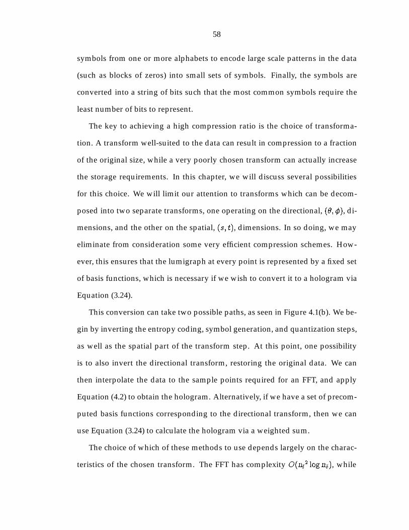
58

symbols from one or more alphabets to encode large scale patterns in the data

(such as blocks of zeros) into small sets of symbols. Finally, the symbols are

converted into a string of bits such that the most common symbols require the

least number of bits to represent.

The key to achieving a high compression ratio is the choice of transforma-

tion. A transform well-suited to the data can result in compression to a fraction

of the original size, while a very poorly chosen transform can actually increase

the storage requirements. In this chapter, we will discuss several possibilities

for this choice. We will limit our attention to transforms which can be decom-

posed into two separate transforms, one operating on the directional, (�; �), di-

mensions, and the other on the spatial, (s; t), dimensions. In so doing, we may

eliminate from consideration some very efficient compression schemes. How-

ever, this ensures that the lumigraph at every point is represented by a fixed set

of basis functions, which is necessary if we wish to convert it to a hologram via

Equation (3.24).

This conversion can take two possible paths, as seen in Figure 4.1(b). We be-

gin by inverting the entropy coding, symbol generation, and quantization steps,

as well as the spatial part of the transform step. At this point, one possibility

is to also invert the directional transform, restoring the original data. We can

then interpolate the data to the sample points required for an FFT, and apply

Equation (4.2) to obtain the hologram. Alternatively, if we have a set of precom-

puted basis functions corresponding to the directional transform, then we can

use Equation (3.24) to calculate the hologram via a weighted sum.

The choice of which of these methods to use depends largely on the charac-

teristics of the chosen transform. The FFT has complexity O(n�2 log n�), while

59

weighted sums is O(n�2n0�), where n0

� � n� is the number of non-negligible

hogel vector coefficients. The cost of the interpolation step required for the

FFT can vary widely depending on the sample points used by the transform.

For a poorly chosen transform, we can have n0

� � n� � n�2, making weighted

sums very inefficient compared to the FFT. However, with a good transform, n0�

can become small enough to make weighted sums faster, especially where in-

terpolation is expensive. This advantage can be further increased by the use of

specialized hardware. While both Equation (4.2) and Equation (3.24) can be effi-

ciently implemented in hardware, this may not be possible for the interpolation

step.

In this chapter, we will provide the details of this flowchart. We will begin by

discussing the sample space used to represent the lumigraph domain. Next we

will describe a number of possible transforms which can be applied to the sam-

pled data. We will then describe the quantization and encoding method which

we developed to convert the transformed data into a compact bit stream. Fi-

nally, we will compare the compression ratios resulting from the various trans-

forms to determine which ones are the most effective for our application.

4.1 Sampling domain

Before selecting a transform, we must first define the set of sample points over

which it will be defined. We choose independent discretizations for the spatial

and directional dimensions. For the (s; t) plane, we will use a regular Carte-

sian grid with sample spacing of d in the s direction and either d or � in the

t direction depending on whether the parallax of the hologram is full or hori-

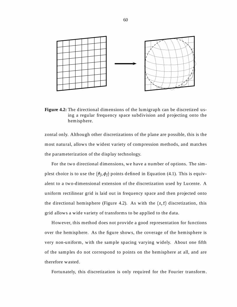
60

Figure 4.2: The directional dimensions of the lumigraph can be discretized us-ing a regular frequency space subdivision and projecting onto thehemisphere.

zontal only. Although other discretizations of the plane are possible, this is the

most natural, allows the widest variety of compression methods, and matches

the parameterization of the display technology.

For the two directional dimensions, we have a number of options. The sim-

plest choice is to use the (�~|; �~|) points defined in Equation (4.1). This is equiv-

alent to a two-dimensional extension of the discretization used by Lucente. A

uniform rectilinear grid is laid out in frequency space and then projected onto

the directional hemisphere (Figure 4.2). As with the (s; t) discretization, this

grid allows a wide variety of transforms to be applied to the data.

However, this method does not provide a good representation for functions

over the hemisphere. As the figure shows, the coverage of the hemisphere is

very non-uniform, with the sample spacing varying widely. About one fifth

of the samples do not correspond to points on the hemisphere at all, and are

therefore wasted.

Fortunately, this discretization is only required for the Fourier transform.

61

We are free to choose a different set of sample points for the lumigraph and, as

discussed briefly above, perform an interpolation when it comes time to do the

conversion. This extra step can add to the computational cost of the conversion,

as well as introduce some small errors into the data, but these costs may be

worth paying in exchange for better compression. Of course, if conversion is

performed using weighted sums, then no interpolation will be necessary except

when the basis fringes are computed as a preprocess.

We have chosen to use a hemicube representation for the directional dimen-

sions (Figure 4.3). This provides significantly more uniform coverage of the

hemisphere than the previous scheme, while maintaining the rectilinear struc-

ture. This mesh is easy to work with, allows rapid interpolation to the sample

points of Equation (4.1), and should already be familiar to computer graphics

programmers. In addition, it can readily be adapted to horizontal-parallax only

holograms, by using a hemisquare, and to holograms with arbitrary viewing

frusta, by adjusting the size of the side and front faces. In particular, for the

common case of holograms with maximum viewing angle � equal or less than

45 degrees, the side faces can be completely eliminated, and the mesh reduces

to a 2D perspective image.

4.2 Transforms

Once a set of discrete sample points for the lumigraph has been chosen, we can

select a pair of transforms to apply to the sampled data, one for the (�; �) di-

mensions, and another for (s; t). As we have already stated, these transforms

form the heart of the compression algorithm. In addition, the (�; �) transform

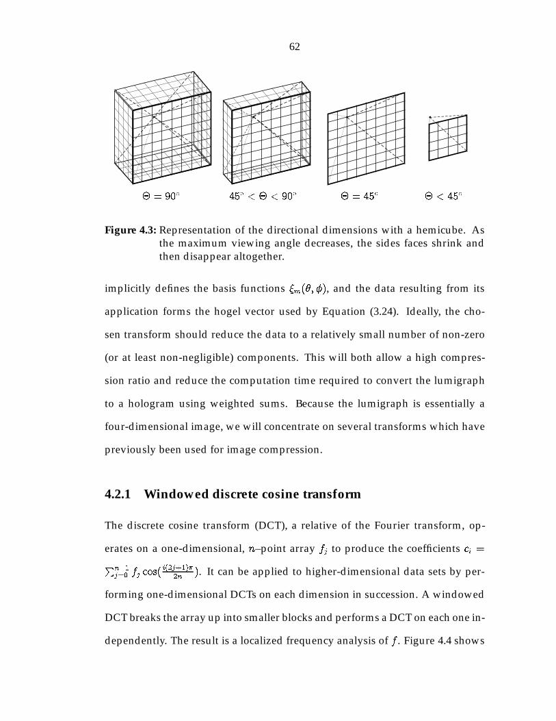
62

b b b b

� = 90� 45� < � < 90� � = 45� � < 45�

Figure 4.3: Representation of the directional dimensions with a hemicube. Asthe maximum viewing angle decreases, the sides faces shrink andthen disappear altogether.

implicitly defines the basis functions �m(�; �), and the data resulting from its

application forms the hogel vector used by Equation (3.24). Ideally, the cho-

sen transform should reduce the data to a relatively small number of non-zero

(or at least non-negligible) components. This will both allow a high compres-

sion ratio and reduce the computation time required to convert the lumigraph

to a hologram using weighted sums. Because the lumigraph is essentially a

four-dimensional image, we will concentrate on several transforms which have

previously been used for image compression.

4.2.1 Windowed discrete cosine transform

The discrete cosine transform (DCT), a relative of the Fourier transform, op-

erates on a one-dimensional, n–point array fj to produce the coefficients ci =Pn�1

j=0 fj cos(i(2j+1)�

2n). It can be applied to higher-dimensional data sets by per-

forming one-dimensional DCTs on each dimension in succession. A windowed

DCT breaks the array up into smaller blocks and performs a DCT on each one in-

dependently. The result is a localized frequency analysis of f . Figure 4.4 shows

63

Figure 4.4: Several of the basis functions generated by the windowed DCT

a few of the basis functions derived from the use of this transform.

This operation lies at the heart of the highly successful JPEG [97, 117] im-

age compression standard, which uses 8-by-8 point DCTs. For any given region

of a typical image, most of the higher frequency (detail) coefficients are likely

to be insignificant, and those which are significant require only a coarse rep-

resentation to provide a perceptually accurate reconstruction. This allows the

transformed image to be represented with significantly fewer bits than the un-

transformed image.

4.2.2 Wavelets

A more sophisticated frequency analysis can be obtained through the use of

wavelet transforms. A comprehensive discussion [28, 29, 36] of wavelet theory

is beyond the scope of this thesis. We will only provide a general overview here.

A wavelet transform uses a pair of one-dimensional analysis filters, ~h and

~g, and a complementary pair of synthesis filters, h and g. Let the original data

array be given by �j0;k, where j0 is some arbitrary fixed value. Then one step of

the wavelet transform generates two arrays half the size of the original:

�j�1;l =Xk

~hk�2l�j;k(4.4)

j�1;l =Xk

~gk�2l�j;k(4.5)

�j�1;l represents a set of average terms, while j�1;l provides detail terms. By

64

repeatedly applying the above equations, we obtain a small array �0 and several

arrays j , for 0 � j � j0. A step of the inverse transform is given by

�j;k =Xl

hk�2l�j�1;l +Xl

gk�2l j�1;l(4.6)

Similarly, through repeated application of this equation, we can obtain the orig-

inal data.

The filters h and g implicitly define two functions, ' and . ', the scaling

function, is given by '(x) =P

k hk'(2x � k), while , the wavelet function, is

given by (x) =P

k gk'(2x � k). The dilations and translations of these func-

tions, 'j;k(x) = '(2jx � k) and j;k(x) = (2jx � k), are the basis functions

corresponding to the transformed coefficients �j;k and j;k, respectively. As j

increases, the functions represent higher frequency details over smaller regions.

This is in contrast to the discrete cosine transform, which does not change scale

as the frequency changes.

For a well chosen set of filters, only a small percentage of the detail terms

will be significant, allowing the data to be compressed. We experimented with

several common wavelets, illustrated in Figures 4.5 through 4.9.

4.2.3 Applying transforms in higher dimensions

2D

As mentioned above, the discrete cosine transform can be applied to a two-

dimensional image by transforming in each dimension independently. That is,

the one-dimensional DCT is applied to each of the rows of the image, and then

subsequently to each of the columns. Wavelet transforms can be applied to a 2D

array in the same way, but the results will not be optimal. Most wavelet-based

65

D2 (Haar) D4 D6

Figure 4.5: Daubechies orthonormal wavelets [35]

(1,1) (1,3) (3,1) (3,3)

Figure 4.6: Average-interpolating wavelets [38, 102]

(2,2) (2,4) (4,2) (4,4)

Figure 4.7: Interpolating wavelets [37, 102]

(3,1) (3,3) (4,2) (4,4)

Figure 4.8: Cohen-Daubechies-Feauveau biorthogonal wavelets [32]

Figure 4.9: (9,7) spline variant wavelet [2]

66

compression algorithms interleave the two transforms to obtain better compres-

sion. We iterate over all j a single time, at each step applying Equations (4.4)

and (4.5) first in one dimension, then the other. In general, the resulting wavelet

functions provide a better fit to the data than those generated by iterating over

each dimension separately.

Hemicube

For the directional dimensions, we must apply a transform to the hemicube.

Since the hemicube is composed of five rectangular faces, we can simply apply

a two-dimensional transform to each face (Figure 4.10). However, in this case,

compression and subsequent decompression can introduce discontinuities at

the boundaries between the faces. We therefore take some additional steps.

We begin by unfolding the hemicube and embedding it in a single 2D array

(Figure 4.11(a)), which is then transformed and compressed. After decompres-

sion, the corner regions are discarded and the hemicube refolded. This elimi-

nates the discontinuities between the front face and the four side faces. How-

ever, it can actually worsen discontinuities between adjacent side faces. Fur-

thermore, it increases the size of the array by one third.

To solve the first problem, we copy a thin strip (8 to 16 pixels wide) from

the edges of the side faces to the opposing edges of the corner regions (Figure

4.11(b)). This provides the desired continuity during compression. Afterwards,

the added data is discarded along with the rest of the corner region.

The second problem is handled by setting the value in the remaining portion

of each corner region to a constant equal to the average over the corresponding

quadrant of the array (Figure 4.11(c)). This ensures that, after the transform is

67

(a)

(b)

Figure 4.10: One way to apply a transform to the hemicube is to separate it intoits individual faces and apply the transform to each.

applied, relatively few additional terms will be needed to represent these re-

gions, despite the increase in the size of the raw data. The only remaining dif-

ficulty lies at the boundary of this constant region, where the sharp edge can

require a relatively large number of terms. To alleviate this, we apply a cubic

interpolation function to the strips added at the edges to smoothly blend them

between the original data and the constant region (Figure 4.11(d)).

This procedure does not guarantee continuity of the function over the hemi-

68

(a) (b)

(c) (d)

Figure 4.11: The hemicube is unfolded into a single array and the corner regionsare filled in so as to eliminate discontinuities caused by compres-sion.

69

cube in any rigorous mathematical sense. However, we have found that, in

practice, it produces a visually smooth representation of the data even at high

compression ratios, while not significantly increasing the compressed data size.

Of course, in the common case where the viewing frustum is less than 45 de-

grees, only the front face is needed, and we can dispense with these extra mea-

sures.

4D

When applying a transform in four dimensions, as with two, better compression

can generally be gained by interleaving all four transforms. However, recall

from Figure 4.1(b) that when the interference pattern is computed via weighted

sums, we only need to perform the inverse transform in the spatial dimensions.

In this case we cannot interleave transformation in the spatial dimensions with

that in the directional ones, and must treat them independently.

4.3 Entropy Coding

Before examining what to do with the data once it has been transformed, let us

skip to the end of the compression process and discuss entropy coding. Suppose

we have a message consisting of a string of symbols from some alphabet. If we

wish to store the message electronically, we can assign a binary number to each

symbol and use these to convert the message into a string of bits. This requires

dlog2(A)e bits per symbol, where A is the size of the alphabet. Entropy coding is

a generic term for a class of algorithms that assign fewer bits to more common

symbols and more bits to rarer symbols, so as to reduce the total size of the

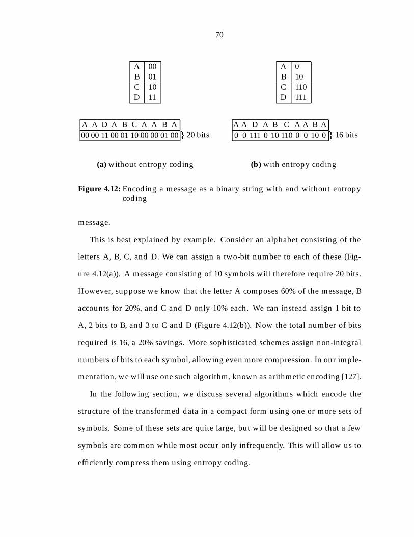
70

A 00B 01C 10D 11

A A D A B C A A B A00 00 11 00 01 10 00 00 01 00 g 20 bits

(a) without entropy coding

A 0B 10C 110D 111

A A D A B C A A B A0 0 111 0 10 110 0 0 10 0 g 16 bits

(b) with entropy coding

Figure 4.12: Encoding a message as a binary string with and without entropycoding

message.

This is best explained by example. Consider an alphabet consisting of the

letters A, B, C, and D. We can assign a two-bit number to each of these (Fig-

ure 4.12(a)). A message consisting of 10 symbols will therefore require 20 bits.

However, suppose we know that the letter A composes 60% of the message, B

accounts for 20%, and C and D only 10% each. We can instead assign 1 bit to

A, 2 bits to B, and 3 to C and D (Figure 4.12(b)). Now the total number of bits

required is 16, a 20% savings. More sophisticated schemes assign non-integral

numbers of bits to each symbol, allowing even more compression. In our imple-

mentation, we will use one such algorithm, known as arithmetic encoding [127].

In the following section, we discuss several algorithms which encode the

structure of the transformed data in a compact form using one or more sets of

symbols. Some of these sets are quite large, but will be designed so that a few

symbols are common while most occur only infrequently. This will allow us to

efficiently compress them using entropy coding.

71

16 11 10 16 24 40 51 6112 12 14 19 26 58 60 5514 13 16 24 40 57 69 5614 17 22 29 51 87 80 6218 22 37 56 68 109 103 7724 35 55 64 81 104 113 9249 64 78 87 103 121 120 10172 92 95 98 112 100 103 99

Figure 4.13: Example quantization table for use in JPEG compression

4.4 Quantization and Symbol Generation

As we have stated, the purpose of the transform is to separate the data into a

few significant components and a large number of insignificant ones. To take

advantage of this for the sake of compression, we need to encode the fact that

these entries are insignificant using a relatively small number of bits. We utilize

two different methods. For the discrete cosine transform, we use a 4D extension

of the JPEG compression scheme, while for the wavelet transforms, we use an

algorithm based on Shapiro’s zerotree encoding.

4.4.1 JPEG-based encoding

As we have discussed, JPEG [97, 117] transforms an image by dividing it into 8-

by-8 blocks and performing a two-dimensional DCT on each one. To encode this

transformed data, each element of each block is divided by the corresponding

element of an integer quantization table, such as the one in Figure 4.13. This

helps compress the data by zeroing out many of the frequency components and

reducing the number of bits required to represent the remaining terms.

This process is lossy, and care must be taken in choosing the quantization

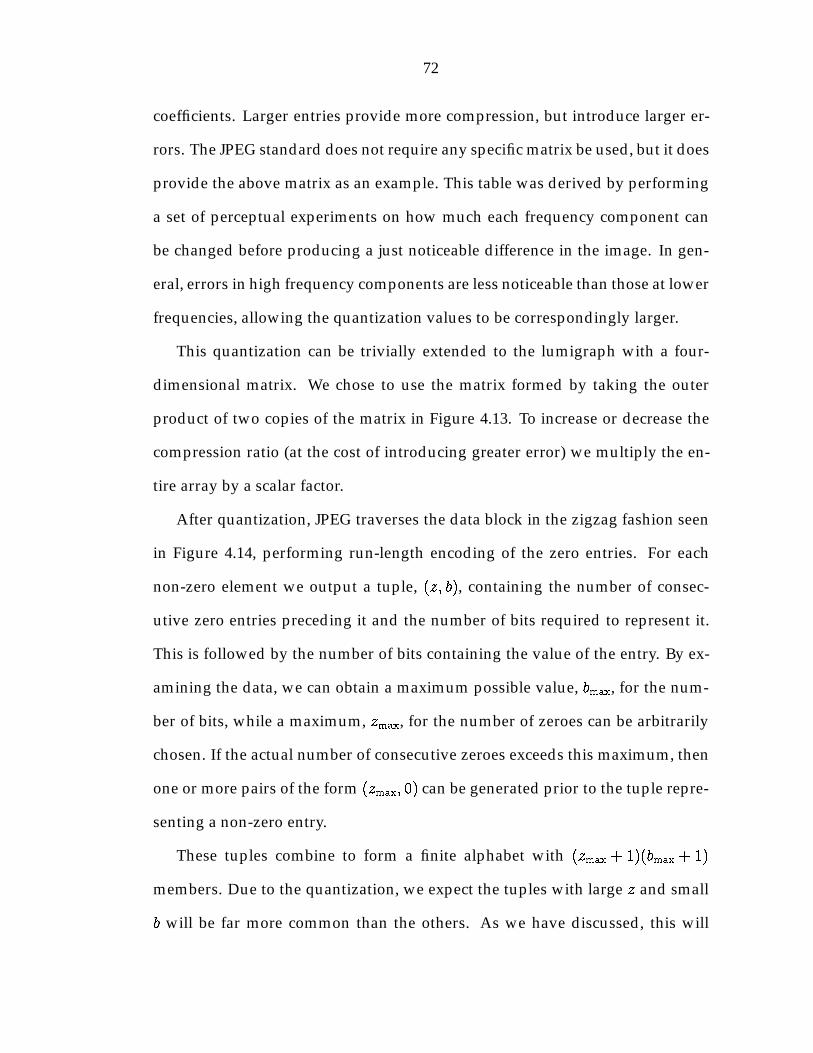
72

coefficients. Larger entries provide more compression, but introduce larger er-

rors. The JPEG standard does not require any specific matrix be used, but it does

provide the above matrix as an example. This table was derived by performing

a set of perceptual experiments on how much each frequency component can

be changed before producing a just noticeable difference in the image. In gen-

eral, errors in high frequency components are less noticeable than those at lower

frequencies, allowing the quantization values to be correspondingly larger.

This quantization can be trivially extended to the lumigraph with a four-

dimensional matrix. We chose to use the matrix formed by taking the outer

product of two copies of the matrix in Figure 4.13. To increase or decrease the

compression ratio (at the cost of introducing greater error) we multiply the en-

tire array by a scalar factor.

After quantization, JPEG traverses the data block in the zigzag fashion seen

in Figure 4.14, performing run-length encoding of the zero entries. For each

non-zero element we output a tuple, (z; b), containing the number of consec-

utive zero entries preceding it and the number of bits required to represent it.

This is followed by the number of bits containing the value of the entry. By ex-

amining the data, we can obtain a maximum possible value, bmax, for the num-

ber of bits, while a maximum, zmax, for the number of zeroes can be arbitrarily

chosen. If the actual number of consecutive zeroes exceeds this maximum, then

one or more pairs of the form (zmax; 0) can be generated prior to the tuple repre-

senting a non-zero entry.

These tuples combine to form a finite alphabet with (zmax + 1)(bmax + 1)

members. Due to the quantization, we expect the tuples with large z and small

b will be far more common than the others. As we have discussed, this will

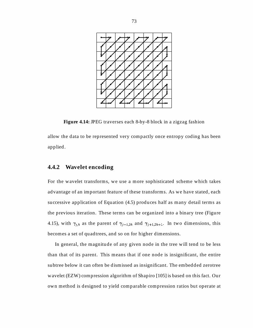
73

b

b

b

b

b

b

b

b

b

b

b

b

b

b

b

b

b

b

b

b

b

b

b

b

b

b

b

b

b

b

b

b

b

b

b

b

b

b

b

b

b

b

b

b

b

b

b

b

b

b

b

b

b

b

b

b

b

b

b

b

b

b

b

b

Figure 4.14: JPEG traverses each 8-by-8 block in a zigzag fashion

allow the data to be represented very compactly once entropy coding has been

applied.

4.4.2 Wavelet encoding

For the wavelet transforms, we use a more sophisticated scheme which takes

advantage of an important feature of these transforms. As we have stated, each

successive application of Equation (4.5) produces half as many detail terms as

the previous iteration. These terms can be organized into a binary tree (Figure

4.15), with j;k as the parent of j+1;2k and j+1;2k+1. In two dimensions, this

becomes a set of quadtrees, and so on for higher dimensions.

In general, the magnitude of any given node in the tree will tend to be less

than that of its parent. This means that if one node is insignificant, the entire

subtree below it can often be dismissed as insignificant. The embedded zerotree

wavelet (EZW) compression algorithm of Shapiro [105] is based on this fact. Our

own method is designed to yield comparable compression ratios but operate at

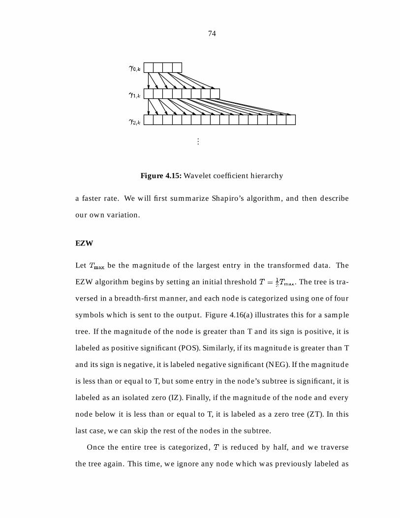
74

0;k

1;k

2;k

...

Figure 4.15: Wavelet coefficient hierarchy

a faster rate. We will first summarize Shapiro’s algorithm, and then describe

our own variation.

EZW

Let Tmax be the magnitude of the largest entry in the transformed data. The

EZW algorithm begins by setting an initial threshold T = 1

2Tmax. The tree is tra-

versed in a breadth-first manner, and each node is categorized using one of four

symbols which is sent to the output. Figure 4.16(a) illustrates this for a sample

tree. If the magnitude of the node is greater than T and its sign is positive, it is

labeled as positive significant (POS). Similarly, if its magnitude is greater than T

and its sign is negative, it is labeled negative significant (NEG). If the magnitude

is less than or equal to T, but some entry in the node’s subtree is significant, it is

labeled as an isolated zero (IZ). Finally, if the magnitude of the node and every

node below it is less than or equal to T, it is labeled as a zero tree (ZT). In this

last case, we can skip the rest of the nodes in the subtree.

Once the entire tree is categorized, T is reduced by half, and we traverse

the tree again. This time, we ignore any node which was previously labeled as

75

-102 -35NEG

3ZT

7-10 5-24

-14ZT

26IZ

-30 8

-42NEG

27ZT

64POS

Output: POS NEG ZT ZT IZ NEG ZT

(a) T = 32

-102 X 3ZT

7-10ZT

5-24NEG

-14ZT

26POS

-30NEG

8ZT

X 27POS

X

Output: POS ZT POS NEG ZT ZT ZT NEG

(b) T = 16

-10NEG

2ZT

X 3ZT

7-10NEG

5X

-14NEG

X X 8ZT

X X

X

Output: NEG ZT ZT NEG ZT NEG

(c) T = 8

Figure 4.16: Several iterations of the main pass of the EZW algorithm

76

significant (Figures 4.16(b) and 4.16(c)). We can repeat this process indefinitely

until every node has been detected as significant.

If we read in these symbols, we obtain an estimate for the value of every ele-

ment of the data set. Given the current threshold T at the time a node is detected

as significant, then the reader knows that its value lies in the interval (T; 2T ] (or

[�2T; T ) for negative significant nodes). To get a better estimate, we add a re-

finement pass between each traversal of the tree. At any given time, based on

the symbols previously generated, we can determine the value of every data

point to within an interval of size T. During the refinement pass, we output, for

each node which has previously been detected as significant, a single bit indi-

cating whether it lies in the upper or lower half of the current bounding interval.

In this way, we obtain a progressively more and more accurate representa-

tion of the data. We continue this until a desired threshold, a maximum output

size, or some more sophisticated stopping condition is met. At this point, a spe-

cial END symbol is generated and the compression halts. This allows a very

high degree of control over the tradeoff between compression ratio and error.

Three-pass method

The iterative refinement provided by the EZW algorithm requires that the en-

tire data array be processed many times. For a two-dimensional image, the time

required is not significant, but in 4D, the cost can be quite prohibitive. We there-

fore desire a new algorithm which provides comparable compression, but with

only a few passes through the data. To achieve this, we will sacrifice our ability

to specify the compression ratio exactly.

As with EZW, we begin by determining the maximum magnitude, Tmax, in

77

the transformed data. Next, we traverse the tree from leaves to root, calculating

two numbers, which we call pt and pn, for each node (Figure 4.17(a)). For a node

with a value of x, pn is calculated as pn =jlog2

�Tmax

jxj

�k. It is equal to the number

of passes that would be required by the EZW algorithm before the node was

detected as significant. pt is set to the minimum value of pn over all members

of the node’s subtree, inclusive. It is equal to the number of EZW passes before

the node is categorized as either significant or an isolated zero.

We traverse the tree again, this time from root to leaves, assigning two new

numbers, �pt and �pn, to the nodes (Figure 4.17(b)). �pt is the difference be-

tween the pt values of the node’s parent and of the node itself. For the purposes

of this computation, the pt value of the root node’s parent is assumed to be zero.

�pn is the difference between the node’s pt value and its pn value. �pt and �pn

encode the same information as pt and pn, but in a relative, rather than absolute

form.

Now let us assume that we have some number of bits, bmax, defining the

accuracy, Tmin =�1

2

�bmax

Tmax, at which the data will be output. We will discuss

how bmax is determined shortly. Given bmax, we can define two finite alphabets,

whose symbols consist of the numbers from �1 to bmax�1, to represent �pt and

�pn.

We traverse the tree one more time, generating a set of symbols for each node

(Figure 4.17(c)). If pn < bmax, the node is significant, and we output the values of

�pt and �pn, a single bit indicating the sign of the node’s value, and bmax�pn�1

bits containing the node’s value quantized by Tmin. (Only bmax � pn � 1 rather

than bmax � pn bits are required because the highest order bit is always 1.) For

a significant leaf node, the symbol for �pn can be omitted, because pn = pt. If

78

-10(2,2)

2(5,5)

-35(0,0)

3(4,4)

7(3,3)

-10(2,2)

5(3,3)

-24(1,1)

-14(2,2)

26(1,0)

-30(1,1)

8(3,3)

-42(0,0)

27(1,1)

64(0,0)

(a) (pt; pn) for each node

-10(0,0)

2(3,0)

-35(0,0)

3(4,0)

7(0,0)

-10(1,0)

5(0,0)

-24(0,0)

-14(2,0)

26(0,1)

-30(0,0)

8(2,0)

-42(0,0)

27(1,0)

64(0,0)

(b) (�pt;�pn) for each node

-10(0)

2(-1)

-35(0)

3(-1)

7-10(1)

5-24(0)

-14(2,0)

26(0,1)

-30(0,0)

8(-1)

-42(0,0)

27(1,0)

64(0,0)

(c) The symbols output for each node given bmax = 3

Figure 4.17: Wavelet tree compression using three-pass method

79

pt < bmax � pn, the node is an isolated zero, and we output the value of �pt and

a special �1 symbol for �pn. Finally, if bmax � pt, the node is a zero tree root.

In this case, we output a �1 for �pt, and we skip processing any nodes in its

subtree.

Recall that the values of the nodes of a subtree tend to be less than the value

of the root. This means that �pn will tend to be zero. Because �pt gives the

node’s pt value relative to that of its parent, it too will tend to be small. This

means that, when entropy coding is applied to the symbols, significant com-

pression will be gained.

We now consider how to select bmax. We construct a histogram h(pn) of the

frequency with which each value pn appears in the data. For any given bmax, a

significant node with a given pn will require bmax�pn bits, plus some overhead to

represent the structure of the tree. If we assume that this overhead is a constant,

c, for all significant nodes, then the entire tree requiresPbmax�1

pn=0h(pn)(bmax�p+c)

bits to represent. For a desired compression ratio, we substitute different values

of bmax into the above equation to find which one yields a compression size that

most closely matches our needs. Only an approximate value is required for c,

and this can be found by experimentation with typical data sets.

In our application, this algorithm yields error vs. compression ratio statistics

roughly equivalent to those of EZW (Figure 4.18), but requires only three passes

through the data set. The first pass determines the value of Tmax. The second

computes pn and pt, and accumulates the histogram h(pn), after which bmax can

be chosen. Finally, the third pass computes �pt and �pn, and generates the out-

put. This speed comes at the cost of the precise control over compression ratio

provided by EZW. Our algorithm only allows the compression to be specified

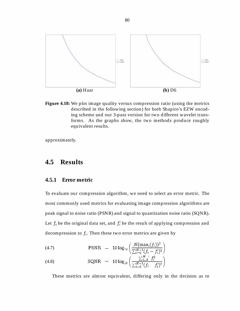
80

EZW

3-pass

(a) Haar

EZW

3-pass

(b) D6

Figure 4.18: We plot image quality versus compression ratio (using the metricsdescribed in the following section) for both Shapiro’s EZW encod-ing scheme and our 3-pass version for two different wavelet trans-forms. As the graphs show, the two methods produce roughlyequivalent results.

approximately.

4.5 Results

4.5.1 Error metric

To evaluate our compression algorithm, we need to select an error metric. The

most commonly used metrics for evaluating image compression algorithms are

peak signal to noise ratio (PSNR) and signal to quantization noise ratio (SQNR).

Let fi be the original data set, and f 0i be the result of applying compression and

decompression to fi. Then these two error metrics are given by

PSNR = 10 log10

N(maxi(fi))

2PN�1i=0 (fi � f 0i)2

!(4.7)

SQNR = 10 log10

PN�1i=0 f

2iPN�1

i=0 (fi � f 0i)2

!(4.8)

These metrics are almost equivalent, differing only in the decision as to

81

whether to use the peak or average value of the data set to normalize the re-

sults. When comparing different compression methods on the same image, this

choice is irrelevant. It only becomes significant when comparing the error across

different images. In this case, SQNR is generally the better option, and is what

we will use for our error metric.

The value of the SQNR has no precise physical meaning. Rather, it serves as

a relative measure by which different compression schemes can be compared.

Most algorithms typically operate in a range between 40 (roughly a 1% error in

each pixel) and 20 (roughly a 10% error).

The SQNR simply measures the total error without regard to the resulting

data’s appearance. Because the human visual system is more sensitive to cer-

tain types of errors, several more sophisticated, perceptually-based error met-

rics have been proposed. However, the problem of extending a perceptual met-

ric for a two-dimensional image to a four-dimensional lumigraph is not trivial.

Recall that the lumigraph consists of numerous 2D images, and that the im-

age seen by someone viewing it is composed of samples drawn from many of

them. It is unclear how perceptually large or small errors in these individual

images may affect the overall view. They may interfere positively to produce

large errors, or negatively to be barely noticeable, and this interaction may vary

depending on the viewer’s position. For this reason, we prefer to rely on the

non-subjective metric provided by the SQNR.

4.5.2 Compression metric

We choose to compute and represent the lumigraph in floating point form,

rather than fixed point, in order to take full advantage of the capabilities of a

82

holographic display system. An ordinary two-dimensional monitor or printer

has a rather narrow dynamic range, allowing images for it to be represented us-

ing only eight bits per color channel. A holographic display is much less limited.

Recall that when we view a point on a hologram, we are actually looking at a

finite region which, although very small, is still composed of many holographic

pixels. The light that reaches our eyes is the result of interference between all of

these pixels. Even if the individual pixels possess only a single bit of resolution,

their combination can have, in theory, a dynamic range of well over a million to

one. Of course, in practice, a real holographic display would be hard-pressed

to achieve this limit. However, we can still expect a potential dynamic range

significantly larger than that of an ordinary monitor, and we therefore choose

not to limit our computed lumigraph to a fixed precision.

This makes the term “compression ratio” somewhat meaningless, since there

is no well-determined size requirement for the original data with which to com-

pare the compressed data. We can, at best, bound the original data by saying

that it lies between eight bits (a typical grey-scale image) and 32 bits (standard

floating point representation) per pixel. Nevertheless, we can still define a met-

ric proportional to compression ratio by using the number of pixels per bit in

the compressed data.

4.5.3 Results

Due to memory constraints, we were unable to apply compression to a full-size

four-dimensional lumigraph. Instead, we used three-dimensional lumigraphs

with 512 samples in U and V , and 128 or 256 samples in s. We tested each of the

transforms on lumigraphs of two models. The first was a simple jack-o-lantern

83

which produces relatively low frequency images; the second was a complex

church model which yields images with more high-frequency details. Errors

were measured over a large range of compression values, from a fraction of a

pixel per bit (no compression) to over 100 ppb (& 1000:1 compression).

The resulting errors are charted in Figures (4.19) and (4.20). For a visual

comparison, Figures (4.21) through (4.28) show the results of compressing the

lumigraphs with each of the transforms to about 8 ppb. These figures show

a single two-dimensional slice of each of the lumigraphs. Recall that in order

to achieve fast compression, we sacrificed our ability to precisely specify the

output size, so it is not possible to apply the different transforms to exactly the

same degree of compression. Nevertheless, they are close enough to allow a

rough comparison. The compression chosen yields a SQNR of roughly 30 for

the better transforms. At this point, errors are becoming noticeable, but the

image quality remains quite high.

As the graphs and images show, the interpolating and average interpolat-

ing wavelets tended to perform better than the other compressors. The highest

overall performance was from the (3,3) average interpolating wavelet, and this

is what we chose to adopt for our needs. In Figure 4.29, we see the affect of

varying the compression rate on the lumigraph quality with this transform.

One issue of which we must take special note is the relatively low perfor-

mance of the JPEG-based compression. It is likely that this is due at least in part

to a poor choice of quantization matrix. A great deal of research is being done

on algorithms for finding the optimal JPEG quantizer for a given image. If such

an optimizer could be adapted to operate on lumigraphs, we expect that signif-

icantly better performance could be achieved. Nevertheless, we do not believe

84

that it would perform as well as the best of the wavelet transforms.

85

20

25

30

35

40

45

50

Compression (ppb)

SQ

NR

Haar

D4

D6

AI (1,3)

AI (3,1)

AI (3,3)

I (2,2)

I (2,4)

I (4,2)

I (4,4)

CDF (3,1)

CDF (3,3)

CDF (4,2)

CDF (4,4)

(9,7)

DCT (JPEG)

1 2 4 8 16 32 64 128

Figure 4.19: Compression statistics for jack-o-lantern

20

25

30

35

40

45

50

Compression (ppb)

SQ

NR

Haar

D4

D6

AI (1,3)

AI (3,1)

AI (3,3)

I (2,2)

I (2,4)

I (4,2)

I (4,4)

CDF (3,1)

CDF (3,3)

CDF (4,2)

CDF (4,4)

(9,7)

DCT (JPEG)

1 2 4 8 16 32 64 128

Figure 4.20: Compression statistics for church

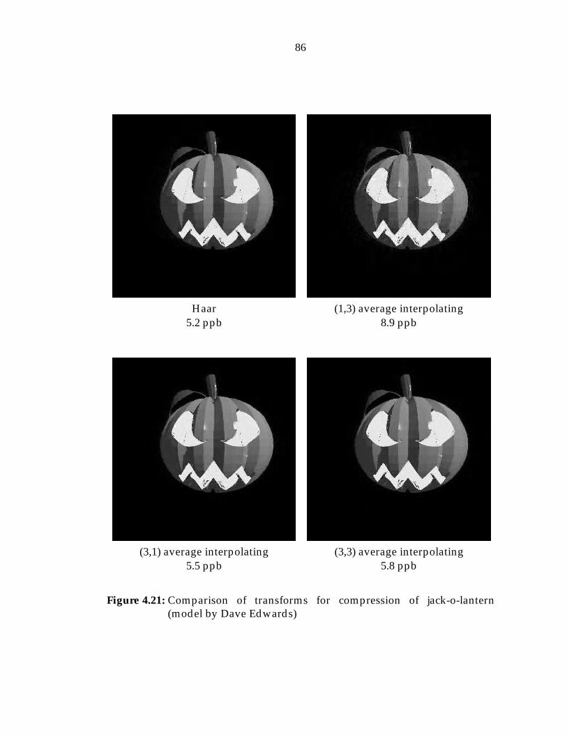
86

Haar (1,3) average interpolating5.2 ppb 8.9 ppb

(3,1) average interpolating (3,3) average interpolating5.5 ppb 5.8 ppb

Figure 4.21: Comparison of transforms for compression of jack-o-lantern(model by Dave Edwards)

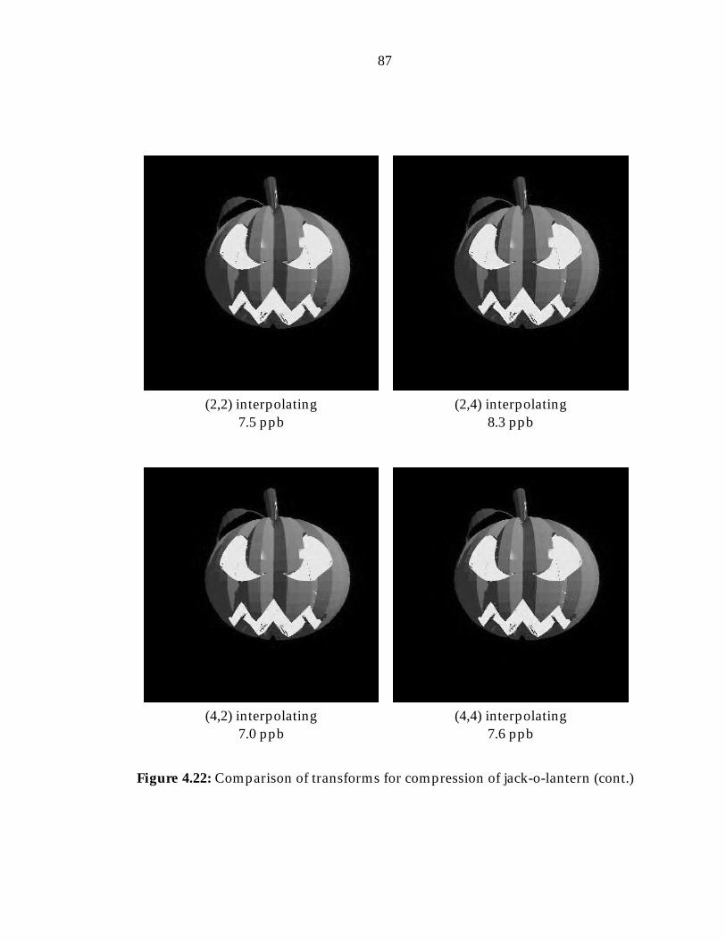
87

(2,2) interpolating (2,4) interpolating7.5 ppb 8.3 ppb

(4,2) interpolating (4,4) interpolating7.0 ppb 7.6 ppb

Figure 4.22: Comparison of transforms for compression of jack-o-lantern (cont.)

88

CDF (3,1) CDF (3,3)11.6 ppb 8.0 ppb

CDF (4,2) CDF (4,4)7.0 ppb 6.7 ppb

Figure 4.23: Comparison of transforms for compression of jack-o-lantern (cont.)

89

Daubechies 4 Daubechies 65.4 ppb 6.4 ppb

(9,7) JPEG7.2 ppb 7.4 ppb

Figure 4.24: Comparison of transforms for compression of jack-o-lantern (cont.)

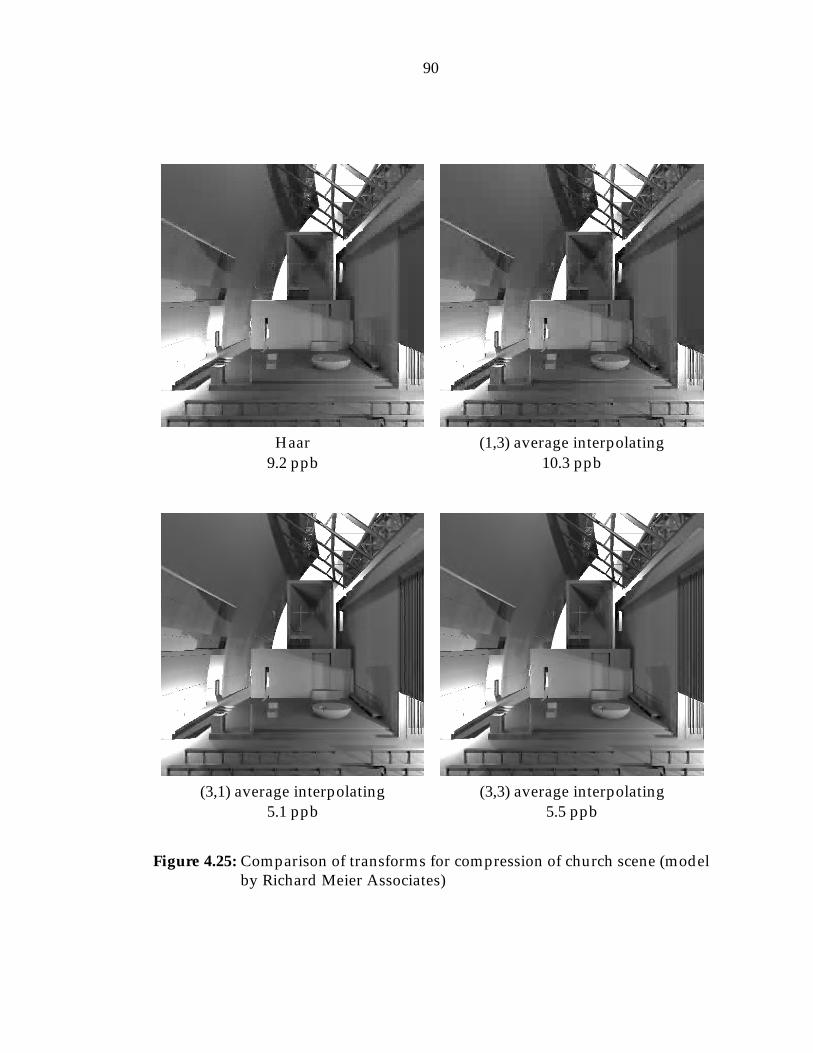
90

Haar (1,3) average interpolating9.2 ppb 10.3 ppb

(3,1) average interpolating (3,3) average interpolating5.1 ppb 5.5 ppb

Figure 4.25: Comparison of transforms for compression of church scene (modelby Richard Meier Associates)

91

(2,2) interpolating (2,4) interpolating6.7 ppb 7.4 ppb

(4,2) interpolating (4,4) interpolating6.3 ppb 6.8 ppb

Figure 4.26: Comparison of transforms for compression of church scene (cont.)

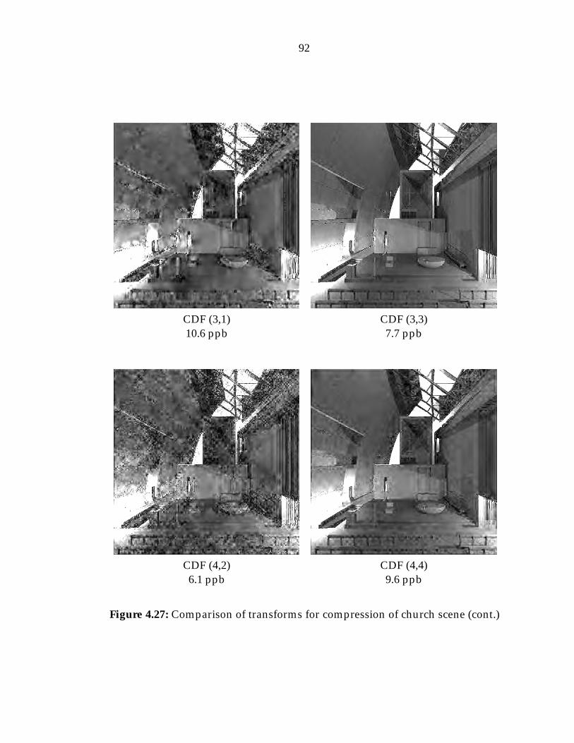
92

CDF (3,1) CDF (3,3)10.6 ppb 7.7 ppb

CDF (4,2) CDF (4,4)6.1 ppb 9.6 ppb

Figure 4.27: Comparison of transforms for compression of church scene (cont.)

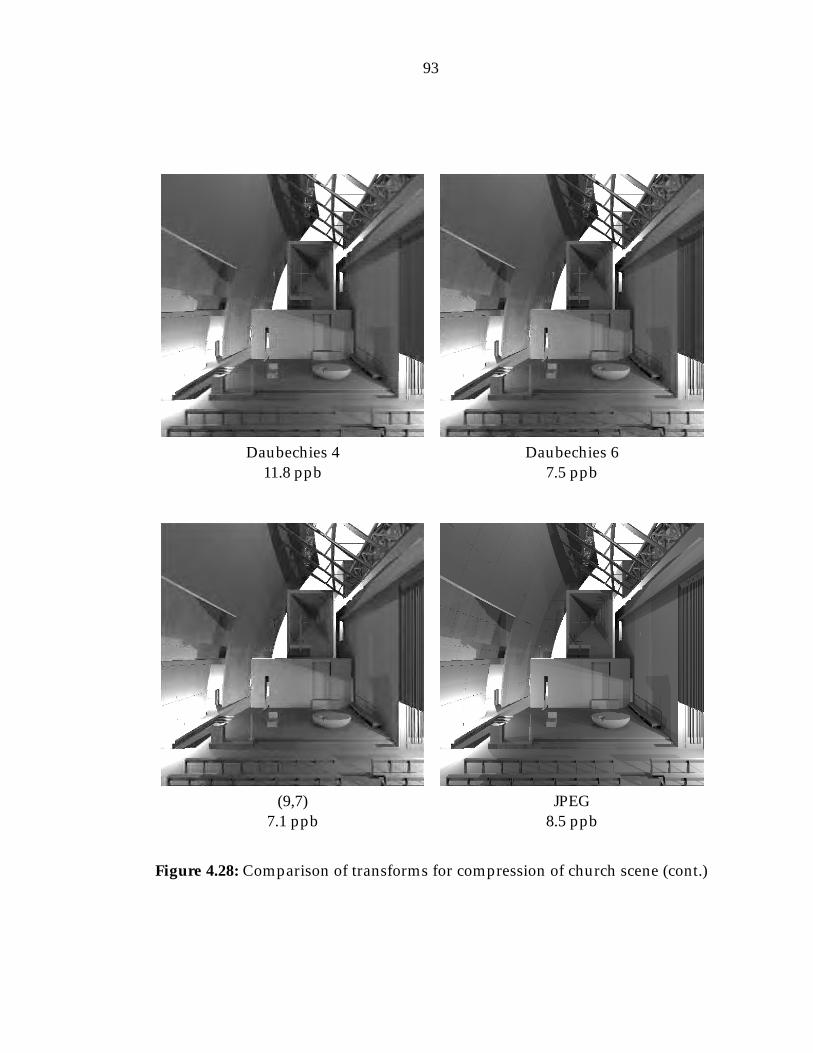
93

Daubechies 4 Daubechies 611.8 ppb 7.5 ppb

(9,7) JPEG7.1 ppb 8.5 ppb

Figure 4.28: Comparison of transforms for compression of church scene (cont.)

94

0.8 ppb 2.5 ppb

5.5 ppb 16.0 ppb

49.6 ppb 147.2 ppb

Figure 4.29: Comparison of lumigraph quality at several degrees of compres-sion using (3,3) average interpolating wavelets applied to thechurch scene

Chapter 5

Rendering

Having determined how we will represent and compress the lumigraph, we

now turn to the problem of computing it. Most previous methods for gener-

ating a lumigraph from a scene description have utilized multiple applications

of standard two-dimensional rendering algorithms. However, in order to make

full use of a holographic display, we must be able to compute a lumigraph at

near real-time rates. This requires rendering speeds orders of magnitude greater

than current methods allow. We can expect that a portion of this deficit will be

eliminated by general improvements in processing power achieved by the time

an electronic holographic display becomes a commercial reality. Nevertheless,

a significant gap will remain, which can only be overcome by developing new

algorithms specifically designed for the four-dimensional case.

The key to reducing rendering time is to take maximum advantage of coher-

ence in the lumigraph to speed or eliminate related and redundant computa-

tions. Previous methods have made use of coherence in only a few dimensions

of the lumigraph. In this chapter, we will develop an algorithm which uses all

four dimensions. Our method parallels, wherever possible, the operations of

95

96

t

Camera Plane s

Focal Plane

V

U

(a) fixed focal plane

V

U

s

tV

(b) local focal plane

Figure 5.1: The lumigraph is parameterized using a camera plane and a focalplane.

the standard rendering pipeline used by most real-time graphics hardware. We

believe it should translate, in a relatively straightforward fashion, into a hard-

ware implementation, allowing it to drive a holographic display system.

5.1 Generalized Lumigraph Rendering

The lumigraph, or light-field, as originally described by Gortler et.al. [46], and

Levoy and Hanrahan [74], consisted of two fixed planes: a camera plane and

a focal plane (Figure 5.1(a)). We discretize these planes with rectangular co-

ordinate grids (s; t) and (U; V ), respectively. The reasons for this odd notation

will become apparent later. The lumigraph is stored as a four-dimensional ar-

ray with data point (s; t; U; V ) receiving the value of the light traveling from the

scene, through point (U; V ), and arriving at point (s; t). We modify the geom-

etry used by Gortler and Levoy slightly by allowing the (U; V ) plane to move

97

so that it is always centered on the current (s; t) point (Figure 5.1(b)). Perceptu-

ally, this will affect the parallax exhibited by the lumigraph. With the original

geometry, objects near the focal plane will tend to maintain a fixed (U; V ) posi-

tion for all (s; t). With ours, as (s; t) changes, objects will tend to move at a rate

inversely proportional to their depth. Note that this choice is made out of con-

venience, not necessity, and that the algorithms discussed in this chapter can be

used, with a few alterations, with either layout. For lumigraphs with less than

a 90 degree viewing frustum, this geometry is equivalent to the sample domain

described in the previous chapter.

To understand what the computation of the lumigraph involves, we consider

the rendering of a single triangle, as illustrated in Figure 5.2. Figure 5.3 shows

the perspective views of the triangle from four points on the camera plane with

fixed t and varying s. As we can see, the image shifts and distorts as s increases.

If we do this for all s and stack the results, we see that the triangle sweeps out

a volume in (s; U; V ) space (Figure 5.4). If we allow t to vary as well, we obtain

a four-dimensional hyper-volume in (s; t; U; V ) space. We refer to this region as

the triangle’s projected volume.

Computing the lumigraph of this triangle requires determining all of the

sample points that lie within the projected volume and setting the value of the

appropriate data point. This process can be viewed as a set of four nested loops,

one for each of the four dimensions. For a scene consisting of many triangles,

we must, in the most naive case, perform this for every polygon, p. Thus, the

basic structure of a lumigraph computation algorithm consists of five nested

loops.

Of course, iterating over all possible combinations of s, t, U , V , and p would

98

x

y

z

s0 s1 s2 s3

Figure 5.2: A triangular polygon positioned in space in front of the cameraplane. It is tilted with respect to the lumigraph so that the top ver-tex is farthest and the bottom is closest. We examine the image seenfrom four points along a single horizontal row on the camera plane.

(a) s0 (b) s1 (c) s2 (d) s3

Figure 5.3: The perspective projection of the polygon as seen from each of thepoints in Figure 5.2. As we move from left to right, the projectionshifts from right to left, and its shape changes due to the varyingdepths of the vertices.

U

V

s

Figure 5.4: The triangle’s projected volume. By stacking the projections from alls, we see that the polygon sweeps out a volume in (s; U; V ) space.If we allow t to vary as well, we obtain a 4-dimensional volume in(s; t; U; V ).

99

be prohibitively expensive. We therefore use a variety of operations, such as

clipping, back-face culling, and spatial subdivision to limit the number of pro-

jection points which must be explicitly evaluated. In addition, when a similar

operation is required for several points, all or part of the computation can be

performed in an outer loop, allowing the results to be reused. By analyzing the

basic structure of a particular lumigraph computation algorithm in terms of the

loop nesting order and how these basic operations fit into the hierarchy, we can

gain an understanding of how well the algorithm takes advantage of coherency.

In the following section, we perform this analysis for several previous methods

for generating lumigraphs.

5.2 Previous Work

In this section, we examine several lumigraph computation algorithms. Note

that we are concerned only with their basic structure. A great number of key

implementation details are omitted for the sake of brevity.

5.2.1 Ray Tracing

Gortler [46] used ray tracing to generate his lumigraphs. Conceptually, this is

perhaps the simplest method available. For each (s; t; U; V ) point, a ray is fired

from (s; t) through (U; V ), and the closest polygon intersection is found. Typi-

cally, some sort of spatial subdivision is used to limit the number of polygons

which must be checked against the ray. This algorithm is summarized in Fig-

ure 5.5. The ordering of the outer loops is of no consequence. The important

observation to make here is that the bulk of the work is performed in the inner-

100

for all (s; t; U; V ) dofor all p0 2 fp0g � fpg determined by spatial subdivision do

if intersect(p0; s; t; U; V )shade(p0; s; t; U; V )

fiod

od

Figure 5.5: Basic structure of ray-tracing based lumigraph computation.

most loops. No effort is made to take advantage of coherence between adjacent

(s; t; U; V ) points.

5.2.2 2D Rendering

Another way to compute the lumigraph is to use multiple applications of a two-

dimensional rendering algorithm (Figure 5.6(a)). We iterate over all points on

the camera plane, generating perspective images for each point, each of which

forms an (s; t) slice of the lumigraph. This allows us to exploit the same coheren-

cies as the 2D routine, and to take advantage of graphics acceleration hardware.

Levoy and Hanrahan [74] computed their light-fields in this way, using Render-

Man to compute the 2D images.

Lucente [85] used a variation of this technique. His holograms had only

horizontal parallax, so they possessed no V dimension. Instead of the making s

and t the outermost loops, he used them as the inner loops (Figure 5.6(b)). For

each V direction, the 2D renderer is used to generate an image with an oblique

projection.

To see how such an algorithm takes advantage of coherency, we will examine

the specific case of a generic z-buffer algorithm following the standard graphics

101

for all (s; t) docompute (U; V ) image with perspective projection

od

(a)

for all V docompute (s; t) image with oblique projection

od

(b)

Figure 5.6: Computing a lumigraph as a series of independent two-dimensionalimages. (a) With (U; V ) as the inner loop, we generate perspectiveimages. (b) With (s; t), we use oblique projections.

pipeline. This is of particular interest to us, since it will later provide the in-

spiration for our own method. An outline of the algorithm is shown in Figure

5.7.

Following the example of Figure 5.6(a), the outermost loop iterates over all

(s; t). For each one, a transformation matrix which converts from world space

to camera space coordinates is constructed. Two-dimensional depth and color

buffers are also initialized.

The enclosed 2D renderer proceeds to iterate over every polygon in the scene.

Each is transformed into camera space, and back-face culling is applied to skip

those not facing the camera point. That portion of the shading computation

which can be interpolated across the polygon is performed at the vertices. The

nature of these computations depends on the shading/lighting models used.

The values obtained can be interpolated to any point on the polygon and used

to determine the light reflected by that point towards the camera.

Next, the polygon is converted into (U; V ) coordinates with a perspective

transformation matrix and clipped against the U and V boundaries of the lumi-

102

for all (s; t)initialize buffersfor all p

transform to camera spaceback-face culling(partial) shadingperspective transformclippingfor all V within polygon bounds

determine intersection of polygon with scan-line Vfor all U within slice bounds

if depth(p; s; t; U; V ) < zbu�er(U; V )complete shading and update buffers

fiod

ododcopy color buffer to lumigraph

od

Figure 5.7: Overview of lumigraph computation with 2D z-buffer.

graph. It is then scan converted to obtain all sample points within its interior.

The depth at each point is compared with the corresponding entry in the depth

buffer. If it is closer, the shading computation is completed and used to set the

color buffer entry, while the depth buffer entry is updated with the new depth

value. Once all points on all polygons have been processed, the color buffer is

copied to the (s; t) slice of the lumigraph, and the process begins again with the

next camera point.

As we can see from the figure, this algorithm takes advantage of coherence

in the (U; V ) dimensions by performing as much of the computation as possible

outside of theU and V loops. It has the additional benefit that z-buffer renderers

are available in hardware for most computers, allowing a moderately efficient

lumigraph renderer to be constructed. Nevertheless, this is still essentially a 2D

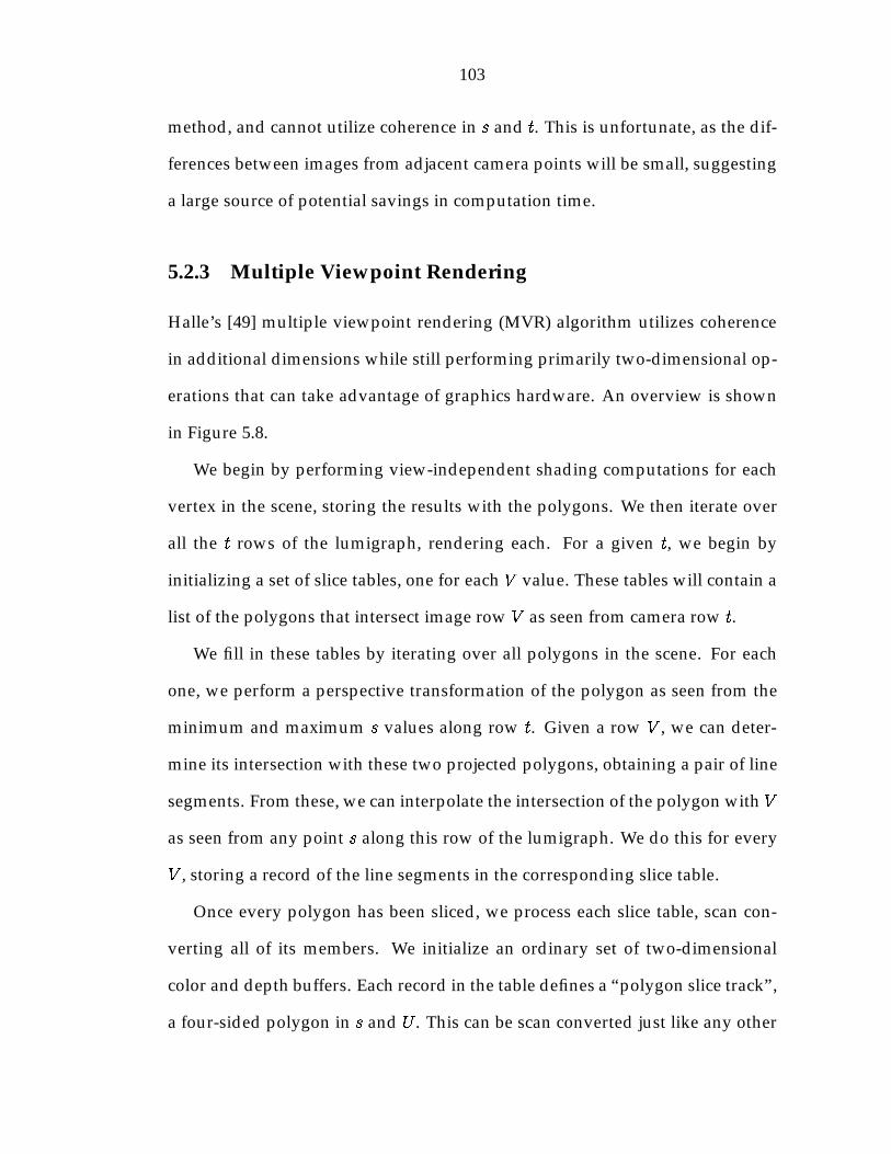
103

method, and cannot utilize coherence in s and t. This is unfortunate, as the dif-

ferences between images from adjacent camera points will be small, suggesting

a large source of potential savings in computation time.

5.2.3 Multiple Viewpoint Rendering

Halle’s [49] multiple viewpoint rendering (MVR) algorithm utilizes coherence

in additional dimensions while still performing primarily two-dimensional op-

erations that can take advantage of graphics hardware. An overview is shown

in Figure 5.8.

We begin by performing view-independent shading computations for each

vertex in the scene, storing the results with the polygons. We then iterate over

all the t rows of the lumigraph, rendering each. For a given t, we begin by

initializing a set of slice tables, one for each V value. These tables will contain a

list of the polygons that intersect image row V as seen from camera row t.

We fill in these tables by iterating over all polygons in the scene. For each

one, we perform a perspective transformation of the polygon as seen from the

minimum and maximum s values along row t. Given a row V , we can deter-

mine its intersection with these two projected polygons, obtaining a pair of line

segments. From these, we can interpolate the intersection of the polygon with V

as seen from any point s along this row of the lumigraph. We do this for every

V , storing a record of the line segments in the corresponding slice table.

Once every polygon has been sliced, we process each slice table, scan con-

verting all of its members. We initialize an ordinary set of two-dimensional

color and depth buffers. Each record in the table defines a “polygon slice track”,

a four-sided polygon in s and U . This can be scan converted just like any other

104

for all pview-independent lighting/shading

odfor all t

initialize slice tablesfor all p

perspective transformfor all V within polygon bounds

slice polygon and add to tableVod

odfor all V

initialize buffersfor all slice tracks in table V

back-face cullingfor all s

determine intersection of slice track with scan-line sfor all U within slice bounds

if depth(p; s; t; U; V ) < zbu�er(s; U)do view-dependent shading and update buffers

fiod

ododcopy color buffer to lumigraph

odod

Figure 5.8: Overview of Halle’s MVR algorithm

polygon. For each interior point, a depth comparison is performed, and if it

passes, view-dependent shading is performed for the point and the buffers are

updated. Once all entries in the slice table have been processed, the color buffer

is copied to the (t; V ) slice of the lumigraph, and we proceed to the next V .

This algorithm takes advantage of coherence in three and four dimensions,

but does so at the cost of requiring additional memory. For example, the view-

independent shading computations are performed only once, instead of once

105

for each value of (s; t), but we need sufficient storage to hold the results for ev-

ery polygon. Perspective transformation and the vertical scanning can be per-

formed once per t, rather than per (s; t), but the transformed and sliced poly-

gons must be kept in slice tables until they are needed. The shading information

requires storage proportional to the number of polygons, while the slice tables

require storage proportional to the number of polygons multiplied by the num-

ber of V slices. Halle utilized existing graphics hardware to implement portions

of his algorithm, but these memory requirements will make it very difficult to

design an efficient, completely hardware-based implementation. The number

of polygons is theoretically unbounded, so unless we place an arbitrary limit

on it, we will need to rely on the computer’s own memory for this additional

storage.

Although this algorithm performs significantly better than that of the previ-

ous section, it still does not take full advantage of coherence in the lumigraph.

Primarily, the t dimension remains largely unexploited. In addition, texture and

shader information for a polygon must be loaded every time a slice of the poly-

gon is processed. This can be done more efficiently if all slices from a polygon

are handled at once. Finally, MVR does not utilize clipping, which can quickly

eliminate many polygons, or portions of polygons, with minimal computation.

5.3 Proposed Algorithm

There is a limit to what can be achieved by adapting existing rendering systems

to the problem of generating a lumigraph. We believe that the only way to per-

form this computation at the speed required by a real-time three-dimensional

106

initialize buffersfor all p

transform to hologram spaceclip to near planeview-independent shading of verticesback-face cullingdetermine projected volumeclipping(partial) view-dependent shading of verticesfor all (s; t; U; V )

if depth(p; s; t; U; V ) < zbu�er(s; t; U; V )complete shading and update buffers

fiod

od

Figure 5.9: General overview of our algorithm. A more detailed description canbe found in Figure 5.21.

display is to develop new hardware and software specifically designed for the

lumigraph. We propose a new algorithm which utilizes a 4D, rather than 2D, z-

buffer. We parallel, as much as possible, the standard rendering pipeline (Figure

5.7), but make use of coherence in all four dimensions. Our goal is to produce an

algorithm which can be implemented in hardware to form the basis of a holo-

graphic graphics accelerator.

Our algorithm’s basic structure is shown in Figure 5.9. The polygon iter-

ation has been made the outermost loop, and the shading, projection, culling,

and clipping operations have been moved with it. Given the current trend to-

wards scenes consisting of many small polygons, these operations account for

the bulk of the computation time required for a polygon. By performing them

on the polygon’s entire projected volume at once, rather than on individual two-

dimensional slices of it, we can obtain significant savings. At the same time, we

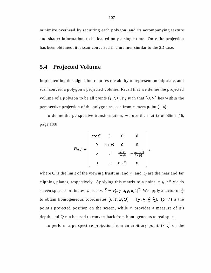
107

minimize overhead by requiring each polygon, and its accompanying texture

and shader information, to be loaded only a single time. Once the projection

has been obtained, it is scan-converted in a manner similar to the 2D case.

5.4 Projected Volume

Implementing this algorithm requires the ability to represent, manipulate, and

scan convert a polygon’s projected volume. Recall that we define the projected

volume of a polygon to be all points (s; t; U; V ) such that (U; V ) lies within the

perspective projection of the polygon as seen from camera point (s; t).

To define the perspective transformation, we use the matrix of Blinn [16,

page 188]

P(0;0) =

2666666666664

cos� 0 0 0

0 cos� 0 0

0 0 sin�

1�znzf

�zn sin�1�

znzf

0 0 sin� 0

3777777777775;

where � is the limit of the viewing frustum, and zn and zf are the near and far

clipping planes, respectively. Applying this matrix to a point [x; y; z]T yields

screen space coordinates [u; v; z0; w]T = P(0;0)[x; y; z; 1]T . We apply a factor of 1

w

to obtain homogeneous coordinates (U; V; Z;Q) = (uw; vw; z

0

w; 1w). (U; V ) is the

point’s projected position on the screen, while Z provides a measure of it’s

depth, and Q can be used to convert back from homogeneous to real space.

To perform a perspective projection from an arbitrary point, (s; t), on the

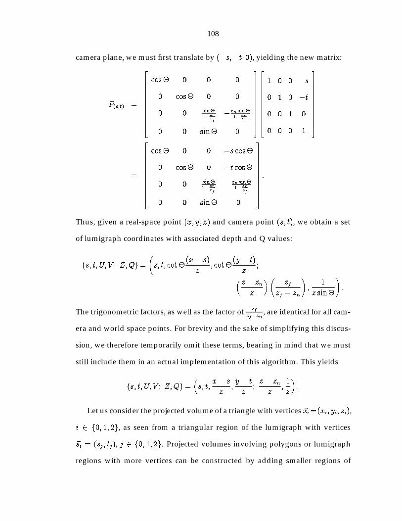
108

camera plane, we must first translate by (�s;�t; 0), yielding the new matrix:

P(s;t) =

2666666666664

cos� 0 0 0

0 cos� 0 0

0 0 sin�

1�znzf

�zn sin�1�

znzf

0 0 sin� 0

3777777777775

2666666666664

1 0 0 �s

0 1 0 �t

0 0 1 0

0 0 0 1

3777777777775

=

2666666666664

cos� 0 0 �s cos�

0 cos� 0 �t cos�

0 0 sin�

1�znzf

�zn sin�1�

znzf

0 0 sin� 0

3777777777775:

Thus, given a real-space point (x; y; z) and camera point (s; t), we obtain a set

of lumigraph coordinates with associated depth and Q values:

(s; t; U; V ; Z;Q) =

s; t; cot�

(x� s)z

; cot�(y � t)z

;

�z � znz

� zf

zf � zn

!;

1

z sin�

!.

The trigonometric factors, as well as the factor of zfzf�zn

, are identical for all cam-

era and world space points. For brevity and the sake of simplifying this discus-

sion, we therefore temporarily omit these terms, bearing in mind that we must

still include them in an actual implementation of this algorithm. This yields

(s; t; U; V ; Z;Q) =�s; t;

x� sz

;y � tz

;z � znz

;1

z

�:

Let us consider the projected volume of a triangle with vertices ~xi=(xi; yi; zi),

i 2 f0; 1; 2g, as seen from a triangular region of the lumigraph with vertices

~si = (sj; tj), j 2 f0; 1; 2g. Projected volumes involving polygons or lumigraph

regions with more vertices can be constructed by adding smaller regions of

109

&~x0

~x1

~x2

~s0

~s1

~s2

~p00

~p01

~p02

~p10

~p11

~p12

~p20

~p21

~p22

Figure 5.10: The projected volume of a triangular polygon as seen from a tri-angular portion of the camera plane. This is a four-dimensionalregion, shown here projected orthographically into 2D.

this form. This volume (Figure 5.10) has nine vertices formed by the projec-

tion of each polygon vertex from each corner of the lumigraph region, ~pij =�sj; tj;

xi�sjzi

;yi�tjzi

; zi�znzi

; 1

zi

�. These vertices are connected by 18 edges of two

different types (Figure 5.11). The first type is formed by the projection of an edge

of the polygon from a corner of the lumigraph, while the second is formed by

a corner of the polygon as seen from an edge of the lumigraph. Similarly, these

edges combine to form 15 faces of three different types (Figure 5.12), which in

turn bound 6 volumes of two types (Figure 5.13). These volumes form the hy-

perfaces of the complete, four-dimensional projected volume.

It is well known that perspective transformations map lines to lines and

polygons to polygons. Therefore, the first type of edge and the first type of

face will be straight and planar, respectively, because they correspond to the

projection of the polygon from a fixed camera point. We can easily see that this

110

(a) (b)

Figure 5.11: Examples of the two types of edges in the projected volume. (a) Apolygon edge seen from a lumigraph vertex. (b) A polygon vertexseen from a lumigraph edge.

(a) (b) (c)

Figure 5.12: Examples of the three types of faces in the projected volume. (a)The polygon as seen from a lumigraph vertex. (b) An edge of thepolygon as seen from an edge of the lumigraph. (c) A vertex of thepolygon as seen from the entire lumigraph.

(a) (b)

Figure 5.13: Examples of the two types of hyperfaces in the projected volume.(a) The polygon as seen from an edge of the lumigraph. (b) An edgeof the polygon as seen from the entire lumigraph.

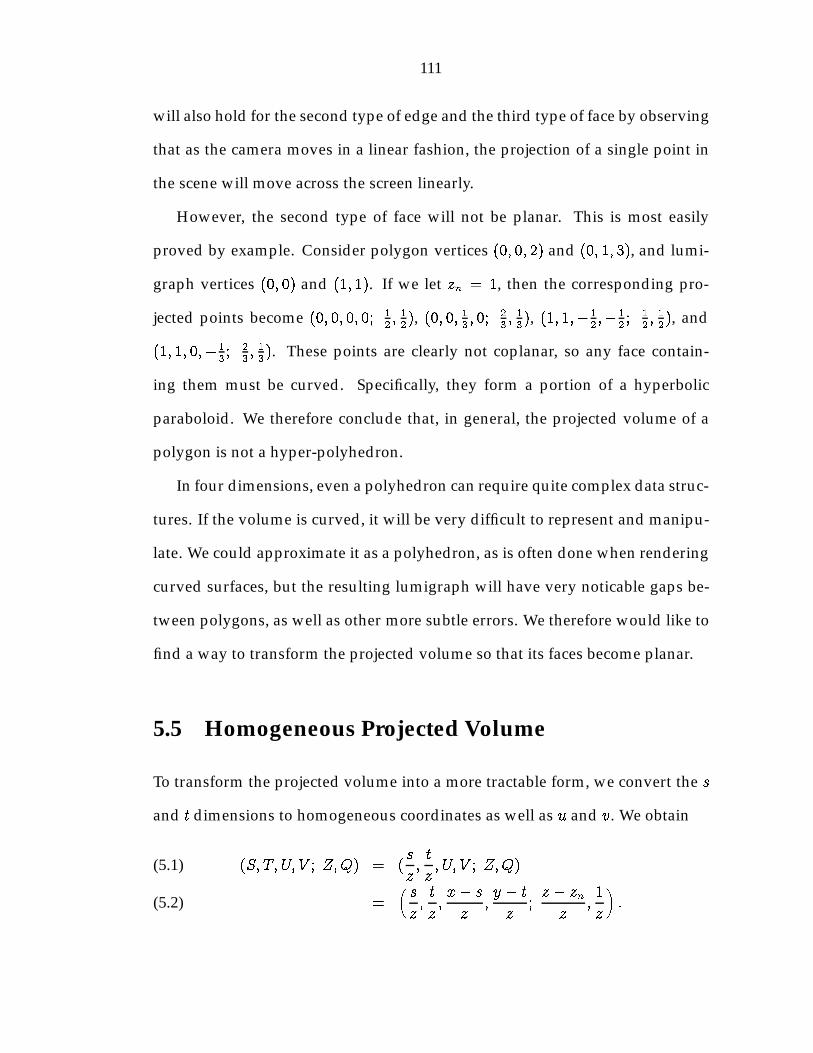
111

will also hold for the second type of edge and the third type of face by observing

that as the camera moves in a linear fashion, the projection of a single point in

the scene will move across the screen linearly.

However, the second type of face will not be planar. This is most easily

proved by example. Consider polygon vertices (0; 0; 2) and (0; 1; 3), and lumi-

graph vertices (0; 0) and (1; 1). If we let zn = 1, then the corresponding pro-

jected points become (0; 0; 0; 0; 1

2; 12), (0; 0; 1

3; 0; 2

3; 13), (1; 1;�1

2;�1

2; 1

2; 12), and

(1; 1; 0;�1

3; 2

3; 13). These points are clearly not coplanar, so any face contain-

ing them must be curved. Specifically, they form a portion of a hyperbolic

paraboloid. We therefore conclude that, in general, the projected volume of a

polygon is not a hyper-polyhedron.

In four dimensions, even a polyhedron can require quite complex data struc-

tures. If the volume is curved, it will be very difficult to represent and manipu-

late. We could approximate it as a polyhedron, as is often done when rendering

curved surfaces, but the resulting lumigraph will have very noticable gaps be-

tween polygons, as well as other more subtle errors. We therefore would like to

find a way to transform the projected volume so that its faces become planar.

5.5 Homogeneous Projected Volume

To transform the projected volume into a more tractable form, we convert the s

and t dimensions to homogeneous coordinates as well as u and v. We obtain

(S; T; U; V ; Z;Q) = (s

z;t

z; U; V ; Z;Q)(5.1)

=�s

z;t

z;x� sz

;y � tz

;z � znz

;1

z

�:(5.2)

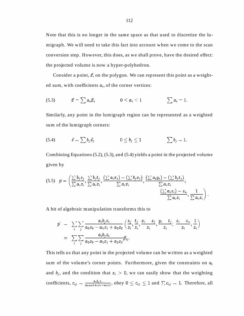
112

Note that this is no longer in the same space as that used to discretize the lu-

migraph. We will need to take this fact into account when we come to the scan

conversion step. However, this does, as we shall prove, have the desired effect:

the projected volume is now a hyper-polyhedron.

Consider a point, ~x, on the polygon. We can represent this point as a weight-

ed sum, with coefficients ai, of the corner vertices:

~x =X

ai~xi 0 � ai � 1X

ai = 1.(5.3)

Similarly, any point in the lumigraph region can be represented as a weighted

sum of the lumigraph corners:

~s =X

bj~sj 0 � bj � 1X

bj = 1.(5.4)

Combining Equations (5.2), (5.3), and (5.4) yields a point in the projected volume

given by

(5.5) ~p =

PbjsjPaizi

;

PbjtjPaizi

;(Paixi)� (

Pbjsj)P

aizi;(Paiyi)� (

Pbjtj)P

aizi;

(Paizi)� znPaizi

;1Paizi

!:

A bit of algebraic manipulation transforms this to

~p =Xi

Xj

aibjzi

a0z0 + a1z1 + a2z2

�sj

zi;tj

zi;xi � sjzi

;yi � tjzi

;zi � znzi

;1

zi

�

=Xi

Xj

aibjzi

a0z0 + a1z1 + a2z2~pij :

This tells us that any point in the projected volume can be written as a weighted

sum of the volume’s corner points. Furthermore, given the constraints on ai

and bj , and the condition that zi > 0, we can easily show that the weighting

coefficients, cij = aibjzia0z0+a1z1+a2z2

, obey 0 � cij � 1 andPcij = 1. Therefore, all

113

point in the projected volume lie inside the polyhedron formed by connecting

the volume’s vertices by linear/planar edges/faces.

Conversely, suppose we have a point, ~p, within this polyhedron. In general,

there are an infinite number of ways to represent this as a weighted sum of the

corner points:

~p =X

cij~pij 0 � cij � 1X

cij = 1.(5.6)

One possible way is to find coefficients a0i and b0j , where 0 � a0i � 1, 0 � b0j � 1,Pa0i =

Pb0j = 1, such that coefficients cij = a0ib

0

j satisfy Equation (5.6). In

regions where the projected volume is degenerate (i.e. when two vertices coin-

cide or where it folds through itself) these coefficients may not be unique, but at

least one solution exists for all possible ~p. From this, we can obtain coefficients,

ai =a0iQi

a00Q0+a

0

1Q1+a

0

2Q2

and bj = b0j , which satisfy Equations (5.3) through (5.5).

This means that they define points in the polygon and lumigraph, respectively,

which together project to ~p. Thus, any point in the polyhedron formed by the

projected volume’s corners is a member of the projected volume.

These two facts combine to prove that the projected volume, in (S; T; U; V )

space, is a polyhedron. These equations further show that the Z and Q values

associated with each point in the volume can be found with the same summa-

tion coefficients. This tells us that these values will vary linearly between any

two points in the projection, just as in the case of an ordinary, two-dimensional,

perspective projection. The depth is not the only thing that can be interpolated

in this way. Again just as with a 2D projection, we can multiply shading, texture

coordinates, or other values by 1

w, interpolate them linearly, and divide by Q to

obtain their value at any point in the projected volume.

The projected volume will either be convex or consist of two convex lobes.

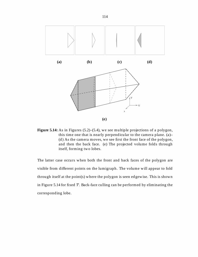
114

(a) (b) (c) (d)

s

V

U

(e)

Figure 5.14: As in Figures (5.2)–(5.4), we see multiple projections of a polygon,this time one that is nearly perpendicular to the camera plane. (a)–(d) As the camera moves, we see first the front face of the polygon,and then the back face. (e) The projected volume folds throughitself, forming two lobes.

The latter case occurs when both the front and back faces of the polygon are

visible from different points on the lumigraph. The volume will appear to fold

through itself at the point(s) where the polygon is seen edgewise. This is shown

in Figure 5.14 for fixed T . Back-face culling can be performed by eliminating the

corresponding lobe.

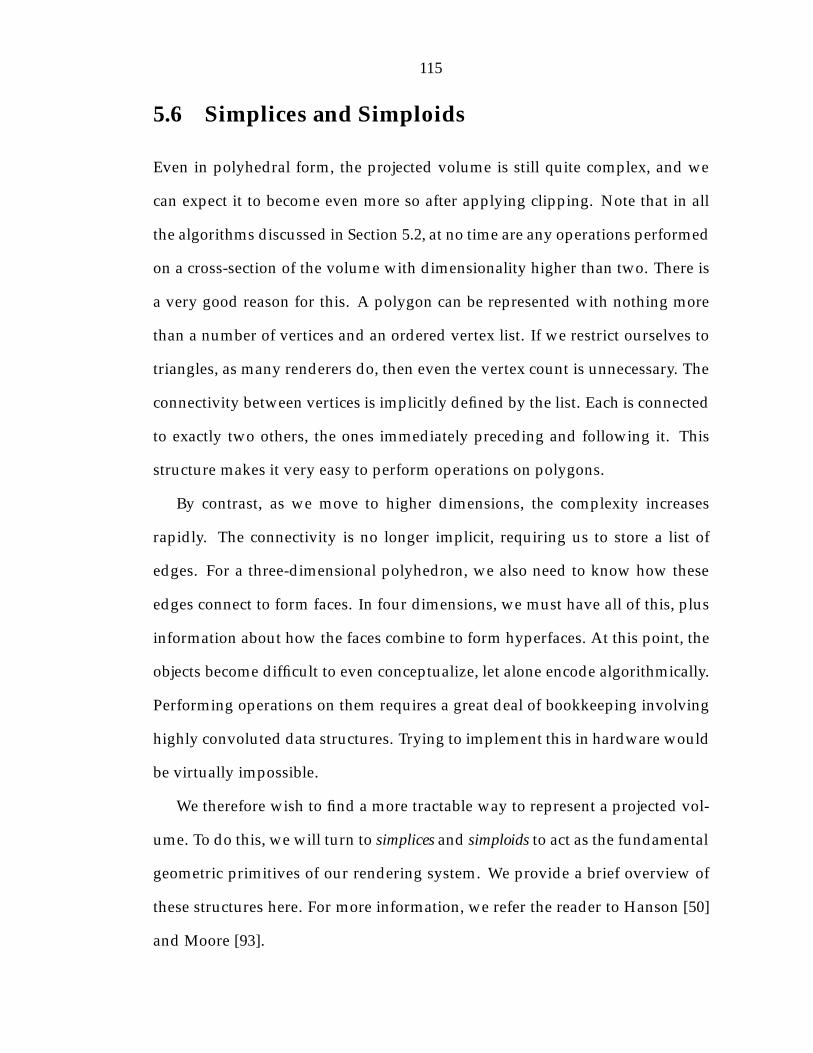
115

5.6 Simplices and Simploids

Even in polyhedral form, the projected volume is still quite complex, and we

can expect it to become even more so after applying clipping. Note that in all

the algorithms discussed in Section 5.2, at no time are any operations performed

on a cross-section of the volume with dimensionality higher than two. There is

a very good reason for this. A polygon can be represented with nothing more

than a number of vertices and an ordered vertex list. If we restrict ourselves to

triangles, as many renderers do, then even the vertex count is unnecessary. The

connectivity between vertices is implicitly defined by the list. Each is connected

to exactly two others, the ones immediately preceding and following it. This

structure makes it very easy to perform operations on polygons.

By contrast, as we move to higher dimensions, the complexity increases

rapidly. The connectivity is no longer implicit, requiring us to store a list of

edges. For a three-dimensional polyhedron, we also need to know how these

edges connect to form faces. In four dimensions, we must have all of this, plus

information about how the faces combine to form hyperfaces. At this point, the

objects become difficult to even conceptualize, let alone encode algorithmically.

Performing operations on them requires a great deal of bookkeeping involving

highly convoluted data structures. Trying to implement this in hardware would

be virtually impossible.

We therefore wish to find a more tractable way to represent a projected vol-

ume. To do this, we will turn to simplices and simploids to act as the fundamental

geometric primitives of our rendering system. We provide a brief overview of

these structures here. For more information, we refer the reader to Hanson [50]

and Moore [93].

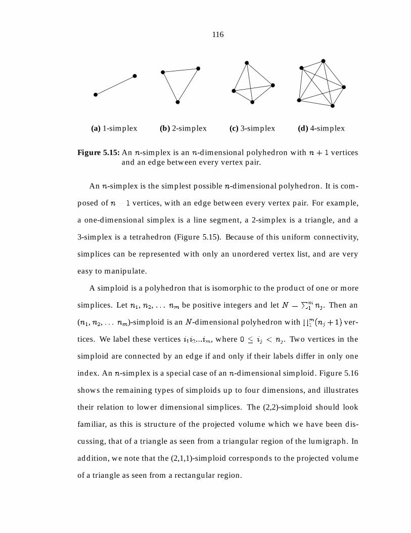
116

(a) 1-simplex (b) 2-simplex (c) 3-simplex (d) 4-simplex

Figure 5.15: An n-simplex is an n-dimensional polyhedron with n + 1 verticesand an edge between every vertex pair.

An n-simplex is the simplest possible n-dimensional polyhedron. It is com-

posed of n + 1 vertices, with an edge between every vertex pair. For example,

a one-dimensional simplex is a line segment, a 2-simplex is a triangle, and a

3-simplex is a tetrahedron (Figure 5.15). Because of this uniform connectivity,

simplices can be represented with only an unordered vertex list, and are very

easy to manipulate.

A simploid is a polyhedron that is isomorphic to the product of one or more

simplices. Let n1, n2, : : : nm be positive integers and let N =Pm

1 nj . Then an

(n1, n2, : : : nm)-simploid is an N -dimensional polyhedron withQm

1 (nj + 1) ver-

tices. We label these vertices i1i2:::im, where 0 � ij < nj . Two vertices in the

simploid are connected by an edge if and only if their labels differ in only one

index. An n-simplex is a special case of an n-dimensional simploid. Figure 5.16

shows the remaining types of simploids up to four dimensions, and illustrates

their relation to lower dimensional simplices. The (2,2)-simploid should look

familiar, as this is structure of the projected volume which we have been dis-

cussing, that of a triangle as seen from a triangular region of the lumigraph. In

addition, we note that the (2,1,1)-simploid corresponds to the projected volume

of a triangle as seen from a rectangular region.

117

1

01

10

00

111

00

(a) (1,1)-simploid

111

0

1 1

0 0

1

000

100

010110

001

101

011

(b) (1,1,1)-simploid

21

0

1

2

0

1

00

10

20

01

11

(c) (2,1)-simploid

1111

1

0 0

1

0

11

0

00000100

1000 1100

00100110

1010

1110

0001

1001

0101

1101

0011

0111

1011

(d) (1,1,1,1)-simploid

2

000

100

200

010

110

001

101

201

011111

211

210

1

0 0

1

0

1

(e) (2,1,1)-simploid

2

0

1

2

01

11

21

00

10

20

02

12

22

0

1

(f) (2,2)-simploid

202

0

1

3 0

1

01

11

21

3110

00 30

(g) (3,1)-simploid

Figure 5.16: A simploid is isomorphic to the product of one or more simplices.

118

5.6.1 Subdivision of a simploid

Any simploid can be subdivided into a set of simplices [93]. The algorithm

for performing this operation for an arbitrary simploid is relatively simple, but

given the rather small number of simploid types that we will be using, and their

low dimension, it is more efficient for us to simply use a lookup table for each

type of simploid. Figure 5.17 provides subdivisions for (2,1,1)-, (2,2)-, and (2,1)-

simploids. These subdivisions are not unique, as can easily seen by examining

the symmetries in the simploids. In general, one might wish to choose between

the possible subdivisions for a given simploid based on some optimization cri-

teria, such as which produces simplices with the lowest eccentricity. However,

in our implementation, we opt to use a single subdivision for all simploids of a

given type.

5.6.2 Clipping and slicing a simplex

Suppose we intersect an n-simplex with a plane, so that n1 vertices lie on one

side of the plane and n2 = n � n1 + 1 lie on the other. The plane divides the

simplex into an (n1, n2�1)-simploid and an (n2, n1�1)-simploid. The region of

intersection is an (n1 � 1, n2 � 1)-simploid. These simploids can be subdivided

into simplices as in the previous subsection. Thus, clipping or slicing a simplex

yields a new set of simplices. Figure 5.18 lists the simplices resulting from the

different ways a 4-simplex can be clipped against a plane. Figure 5.19 and Figure

5.20 show the results of taking a slice of a 4- or 3-simplex, respectively.

119

210

000

100

200

010

110

001

101

201

011111

211

(000, 001, 011, 111, 211)(000, 001, 101, 111, 211)(000, 001, 101, 201, 211)(000, 010, 011, 111, 211)(000, 010, 110, 111, 211)(000, 010, 110, 210, 211)(000, 100, 101, 111, 211)(000, 100, 101, 201, 211)(000, 100, 110, 111, 211)(000, 100, 110, 210, 211)(000, 100, 200, 201, 211)(000, 100, 200, 210, 211)

(a) Subdivision of a (2,1,1)-simploid into twelve 4-simplices

2201

11

21

00

10

20

02

12(00, 01, 02, 12, 22)(00, 01, 11, 12, 22)(00, 01, 11, 21, 22)(00, 10, 11, 12, 22)(00, 10, 11, 21, 22)(00, 10, 20, 21, 22)

(b) Subdivision of a (2,2)-simploid into six 4-simplices

2100

10

20

01

11 (00, 01, 11, 21)(00, 10, 11, 21)(00, 10, 20, 21)

(c) Subdivision of a (2,1)-simploid into three 3-simplices

Figure 5.17: The three types of simploids which our algorithm uses and theircorresponding subdivision into sets of simplices.

120

U

a

b

d

e

c

(a)

e

a

b

c

d(a, ab, ac, ad, ae)

e

a

b

c

d(a, ac, ad, ae, be)(a, ac, ad, bd, be)(a, ac, bc, bd, be)(a, b, bc, bd, be)

e

a

b

c

d

(a, ad, ae, be, ce)(a, ad, bd, be, ce)(a, ad, bd, cd, ce)(a, b, bd, cd, ce)(a, b, bd, be, ce)(a, b, c, cd, ce)

e

a

b

c

d

(a, b, c, d, de)(a, b, c, ce, de)

(a, b, be, ce, de)(a, ae, be, ce, de)

(b)

Figure 5.18: Clipping of a 4-simplex is shown here for the specific case of theupper U clipping plane. The other planes are handled similarly.(a) The vertices are sorted in order of increasing U , and labeled‘a’ through ‘e’. (b) We assign label ‘ab’ to the point at which theplane intersects the edge between a and b, and so on for all thevertex pairs. Depending on the number of vertices inside the plane,different sets of simplices result, as shown.

121

e

a

b c d

(ab, ac, ad, ae)

e

a b

c d

(ac, ad, ae, be)(ac, ad, bd, be)(ac, bc, bd, be)

e

a b c

d

(ad, bd, cd, ce)(ad, bd, be, ce)(ad, ae, be, ce)

e

a b c d

(ae, be, ce, de)

Figure 5.19: Slicing a 4-simplex yields one or three 3-simplices.

d

a

b

cd

a

b

cd

a

b

c

(ab, ac, ad) (ac, ad, bd, bc) (ad, bd, cd)

Figure 5.20: Slicing a 3-simplex yields a triangle or quadrilateral.

5.7 Complete Algorithm

We are now ready to discuss our algorithm (Figure 5.21) in detail. We begin

by initializing a set of four-dimensional depth and color buffers. We then iterate

over each triangle in the scene, transforming it into hologram space and clipping

it the the near plane. Depending on the shading model, all or part of the view-

independent shading computation is now performed at the triangle’s vertices.

5.7.1 Projection / Back-face culling

Next, we compute the projected volume while performing back-face culling.

Recall from Figure 5.14 that, when both the front and back faces of the polygon

122

initialize buffersfor all p

transform to hologram spaceclip to near planeview-independent shading of verticesdetermine projected volume with back-face cullingpartial view-dependent shadingsubdivide into queue of 4-simplicesfor all members of queue

clip against U and V boundsodfor all members of queue

for all V within simplex boundsslice 4-simplex at V , generating queue of 3-simplicesfor all 3-simplices

for all U within simplex boundsslice 3-simplex at U , generating one or two trianglesfor each triangle

convert from (S; T ) to (s; t)for all t within triangle bounds

determine endpoints for slice at tfor all s within slice

if depth(p; s; t; U; V ) < zbu�er(s; t; U; V )complete shading and update buffers

fiod

odod

odod

odod

od

Figure 5.21: Our complete rendering algorithm.

123

are visible from different points on the lumigraph, the projected volume can

fold through itself, yielding front- and back-face lobes. The region at which this

fold occurs corresponds to the points on the lumigraph at which the polygon is

seen edge on. This is simply the line at which the polygon and camera planes

intersect. We can therefore perform back-face culling by considering only the

lumigraph region on the appropriate side of this line.

Figure 5.22 illustrates the five basic cases for this line to cross the lumigraph’s

(s; t) range. If the entire range is in the back-face half-plane, the triangle is

culled. Otherwise, we obtain a triangular or quadrilateral lumigraph region,

or a five-sided region which can be split into one of each of these two types.

Given a triangular polygon, these regions will produce projected volumes that

are (2,2)- and (2,1,1)-simploids, respectively.

We compute the projection of the triangle’s vertices from each of the corners

of this region to obtain the vertices of the projected volume. Again depending

on the shading model, those portions of the view-dependent shading which

can be interpolated between viewpoints are now computed for each projection

point. We then use the subdivision scheme defined in Section 5.6.1 to convert

the projected volume into a queue of 4-simplices. The resulting simplices are

listed in Figure 5.22.

5.7.2 Clipping

Next, we iterate four times over the queue we have created, performing clipping

for each of the U and V boundaries of the lumigraph. During the first iteration,

any simplex which lies entirely outside the upper U bound is simply discarded,

while any that lies entirely inside is left alone. Those that intersect the edge

124

regionbackfaceregion

frontface polygon discarded

A B

C(A0, A1, A2, B2, C2)(A0, A1, B1, B2, C2)(A0, A1, B1, C1, C2)(A0, B0, B1, C1, C2)(A0, B0, B1, B2, C2)(A0, B0, C0, C1, C2)

A B

C D(A0, A1, A2, B2, D2) (A0, A1, A2, C2, D2)(A0, A1, B1, B2, D2) (A0, A1, B1, D1, D2)(A0, A1, C1, C2, D2) (A0, A1, C1, D1, D2)(A0, B0, B1, B2, D2) (A0, B0, B1, D1, D2)(A0, B0, D0, D1, D2) (A0, C0, C1, C2, D2)(A0, C0, C1, D1, D2) (A0, C0, D0, D1, D2)

A

B

C

D

E

(A0, A1, A2, B2, C2) (A0, A1, B1, B2, C2)(A0, A1, B1, C1, C2) (A0, B0, B1, C1, C2)(A0, B0, B1, B2, C2) (A0, B0, C0, C1, C2)(B0, B1, B2, C2, E2) (B0, B1, B2, D2, E2)(B0, B1, C1, C2, E2) (B0, B1, C1, E1, E2)(B0, B1, D1, D2, E2) (B0, B1, D1, E1, E2)(B0, C0, C1, C2, E2) (B0, C0, C1, E1, E2)(B0, C0, E0, E1, E2) (B0, D0, D1, D2, E2)(B0, D0, D1, E1, E2) (B0, D0, E0, E1, E2)

A B

C D(A0, A1, A2, B2, D2) (A0, A1, A2, C2, D2)(A0, A1, B1, B2, D2) (A0, A1, B1, D1, D2)(A0, A1, C1, C2, D2) (A0, A1, C1, D1, D2)(A0, B0, B1, B2, D2) (A0, B0, B1, D1, D2)(A0, B0, D0, D1, D2) (A0, C0, C1, C2, D2)(A0, C0, C1, D1, D2) (A0, C0, D0, D1, D2)

Figure 5.22: Back-face culling is performed by determining where the plane ofthe polygon intersects the camera plane. If the lumigraph regionlies entirely in the back-face half-plane, the polygon is discarded.Otherwise, the projected volume of the polygon (whose vertices arelabeled 0 through 2) is found as seen from the portion of the lumi-graph within the front-face half-plane. Depending on the numberof vertices of this region, the projected volume is split into 6, 12, or18 4-simplices, as shown.

125

are clipped as per Section 5.6.2, and replaced in the queue by a new set with

between one and six simplices. This process is then repeated for the lower U

bound and both V bounds.

5.7.3 Scanning in U and V

We now proceed to iterate over every simplex in the queue, scan converting

them into the buffers. For each one, we sort its vertices in order of increasing V .

This separates the simplex into 4 regions between each pair of vertices. In each

of these intervals, we increment over all integral values of V , slicing as in Figure

5.19, obtaining a new queue of one or three 3-simplices.

We perform a similar process on the 3-simplices. The vertices of each one

is sorted in order of increasing U . We then iterate over all U values within the

simplex’s range, slicing as in Figure 5.20 to obtain one or two triangles.

5.7.4 Scanning in s and t

Before we scan convert these triangles, we must convert them from homoge-

neous (S; T ) coordinates to the (s; t) coordinates used to discretize the lumi-

graph by dividing them by their associated Q value. Unfortunately, after this

transformation the triangle is no longer polygonal (Figure 5.23). However, the

curves that form its edges are constrained in such a way that it will still be pos-

sible to scan convert it in a manner similar to an ordinary polygon.

Let (S0; T0; Z1; Q0) and (S1; T1; Z1; Q1) be the endpoints of a line segment in

126

2S

T

0

1

(a)

1t

s

2

0

(b)

Figure 5.23: (a) A polygon in (S; T ) space (b) becomes curved when convertedback to (s; t).

(a) (b)

Figure 5.24: (a) The curves bounding the polygon will monotonically increaseor decrease in s and t. (b) Curves containing local minima or max-ima in s and/or t, such as these, will not occur. We can thereforescan vertically or horizontally from one endpoint to the other andbe guaranteed that each scan-line will intersect the curve exactlyonce.

1t

s

2

0

(a)

2S

T

0

1

(b)

Figure 5.25: (a) We scan across the curved shape for each value of t. (b) Eachscan-line becomes a curve in (S; T ).

127

(S; T ) space. Then in (s; t) space, the line becomes

(5.7) (s; t; Q;Z) =

a0S0 + (1� a0)S1a0Q0 + (1� a0)Q1

;a0T0 + (1� a0)T1a0Q0 + (1� a0)Q1

;

a0Z0 + (1� a0)Z1; a0Q0 + (1� a0)Q1)

where a0 ranges from 0 to 1. This curve is guaranteed to monotonically increase

or decrease in both s and t. That is, it will not form any local maxima or minima

(Figure 5.24).

This fact allows us to scan convert the transformed triangle in a relatively

straightforward fashion. We convert the vertices of the triangle into (s; t) space,

determine the maximum and minimum t values, and proceed to iterate over all t

within this interval (Figure 5.25). At each one, we find the points of intersection

between this slice and the shape’s edges. To do this, we must solve for a0 in

Equation (5.7) for the given value of t. This yields

a0 =tQ1 � T1

(tQ1 � T1)� (tQ0 � T0)

We use this to find the values of s where the edges cross the slice, as well as to

interpolate the depth and other associated values at these points.

Once the endpoints of the slice have been found, we iterate over all s within

the slice, comparing the depth at each point with the current value in the depth

buffer, and, if necessary, shading these points and entering their values into the

color buffer. However, we cannot linearly interpolate the depth values between

the two endpoints as we can in the case of an ordinary polygon, because a scan

line in (s; t) space corresponds to a curve in (S; T ), If we represent a point on

the triangle as a weighted sum of the vertices with coefficients ai, such that

a0 + a1 + a2 = 1, then the corresponding (s; t) point is given by

(s; t; Q; Z) =

PaiSiPaiQi

;

PaiTiPaiQi

;X

aiZi;X

aiQi

!.

128

Inverting this yields

a0 =a00

a00 + a01 + a02a1 =

a01a00 + a01 + a02

a2 =a02

a00 + a01 + a02

a00 = t01s0

2 � t0

2s0

1 a01 = t02s0

0 � t0

0s0

2 a02 = t00s0

1 � t0

1s0

0

s0i = Si � sQi

t0i = Ti � tQi.

Using these coefficients, we can interpolate the correct depth for a given (s; t)

point, as well as the shading, texture coordinates, and any other desired values.

This process makes the inner loop more computationally expensive than in the

case of ordinary 2D scan conversion, but not excessively so.

5.8 Results

We implemented our algorithm on an IBM SP2 cluster consisting of 120 and

135 MHz processors, each with between 256 and 2048 MB of RAM. Although in

practice we use coarse-grained parallelism to speed the computation, the times

given here are for a single 120 MHz processor. For comparison, we also pro-

duced software to compute the lumigraph using repeated applications of an

ordinary two-dimensional zbuffer. In addition, we implemented a version of

our algorithm which scan converts 3-simplices into a three-dimensional buffer.

It exploits coherence in the s, U , and V dimensions, but treats each t slice in-

dependently, and is suitable for horizontal parallax only holograms. We can

expect its performance to be somewhere between that of the 2D and 4D cases.

We tested this software on five models of varying complexity. For each one,

we generated lumigraphs with a size of 360�360 samples in (s; t), and either

129

256�256 or 512�512 in (U; V ). Due to memory constraints, it was not possible

to generate the entire lumigraph at once. Instead, the (s; t) dimensions were

divided into square regions and the 4D zbuffer was applied to each one inde-

pendently. The size of these regions was varied and the resulting computation

times are plotted in the graphs shown in Figures (5.26) through (5.30). The hori-

zontal axis provides the size of each side of the (s; t) regions, so the total number

of samples is given by the square of this number. The vertical axis plots the av-

erage cost for each (U; V ) sub-image of the lumigraph (i.e. a single (s; t) point).

We also subdivided (s; t) into linear regions to test the application of the 3D

algorithm.

As the graphs show, when applied to a region of size one, our algorithm is

considerably more expensive than scan converting in two dimensions. How-

ever, as the number of camera points increases, this additional cost is quickly

amortized over the entire region. The computation time drops significantly, be-

fore eventually leveling off.

The degree of improvement over two-dimensional scan conversion depends

primarily on two factors. The most significant is the cost of the shading opera-

tion which must be performed for each visible surface point. This computation

forms the heart of the innermost loops of the algorithm, and the total time re-

quired for it is fixed regardless of whether 2D or 4D scan conversion is used. If

this cost is large relative to that of the rest of the computation, few savings will

be obtained. On the other hand, if shading can be performed very quickly, then

our method becomes much more efficient.

This is most easily observed by comparing Figures (5.26) and (5.27). These

show the same scene shaded by two very different methods. The model in Fig-

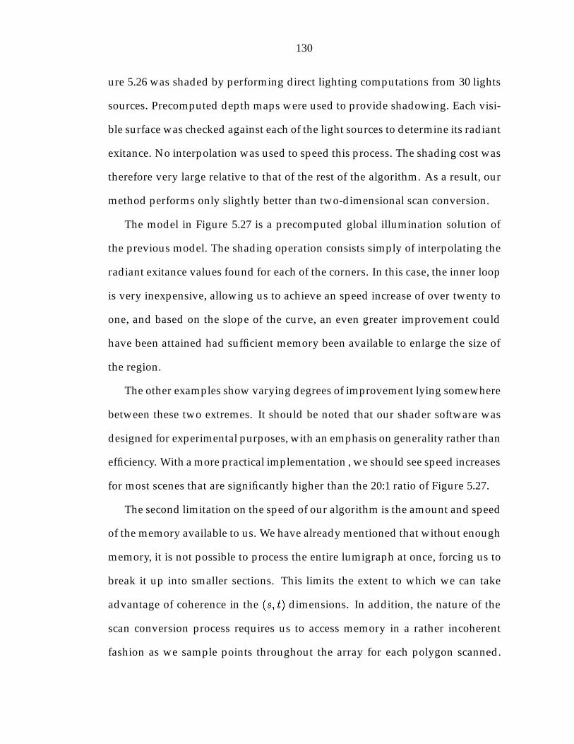
130

ure 5.26 was shaded by performing direct lighting computations from 30 lights

sources. Precomputed depth maps were used to provide shadowing. Each visi-

ble surface was checked against each of the light sources to determine its radiant

exitance. No interpolation was used to speed this process. The shading cost was

therefore very large relative to that of the rest of the algorithm. As a result, our

method performs only slightly better than two-dimensional scan conversion.

The model in Figure 5.27 is a precomputed global illumination solution of

the previous model. The shading operation consists simply of interpolating the

radiant exitance values found for each of the corners. In this case, the inner loop

is very inexpensive, allowing us to achieve an speed increase of over twenty to

one, and based on the slope of the curve, an even greater improvement could

have been attained had sufficient memory been available to enlarge the size of

the region.

The other examples show varying degrees of improvement lying somewhere

between these two extremes. It should be noted that our shader software was

designed for experimental purposes, with an emphasis on generality rather than

efficiency. With a more practical implementation , we should see speed increases

for most scenes that are significantly higher than the 20:1 ratio of Figure 5.27.

The second limitation on the speed of our algorithm is the amount and speed

of the memory available to us. We have already mentioned that without enough

memory, it is not possible to process the entire lumigraph at once, forcing us to

break it up into smaller sections. This limits the extent to which we can take

advantage of coherence in the (s; t) dimensions. In addition, the nature of the

scan conversion process requires us to access memory in a rather incoherent

fashion as we sample points throughout the array for each polygon scanned.

131

This causes a great deal of memory page swapping, which can slow down the

computation. As a result, the time plots in the figures level off at a higher point

than they would if memory access were not a concern, and some even begin to

increase as the memory becomes completely full.

Therefore, in order to take full advantage of our algorithm, we require a

very large amount of fast random access memory. While this requirement is

still somewhat beyond the limits of current technology, it is not unreasonable.

Recall that our goal is to provide an algorithm which can drive an electronic

holographic display system, and that, as large as the lumigraph is, a hologram

is even larger. A frame buffer for such a display would need even more memory

than we have described. Therefore, it is safe to assume that by the time a holo-

graphic display becomes commercially available, the memory which we need

to efficiently implement our rendering algorithm will be available as well.

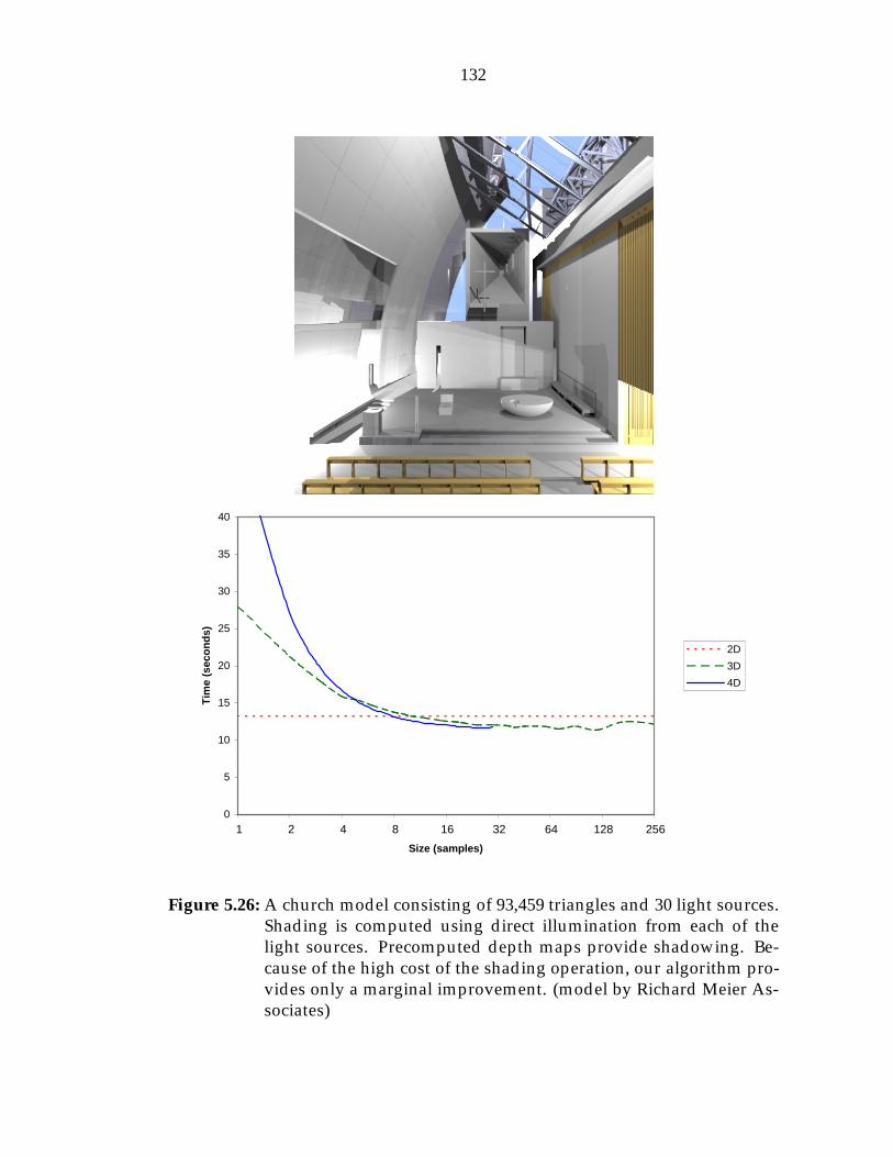
132

0

5

10

15

20

25

30

35

40

Size (samples)

Tim

e (s

eco

nd

s)

2D

3D

4D

1 2 4 8 16 32 64 128 256

Figure 5.26: A church model consisting of 93,459 triangles and 30 light sources.Shading is computed using direct illumination from each of thelight sources. Precomputed depth maps provide shadowing. Be-cause of the high cost of the shading operation, our algorithm pro-vides only a marginal improvement. (model by Richard Meier As-sociates)

133

0

100

200

300

400

500

600

Size (samples)

Tim

e (s

eco

nd

s)

2D

3D

4D

1 2 4 8 16 32 64 128 256

Figure 5.27: A global illumination solution of the same scene as in the previousfigure, consisting of 3,320,101 triangles with radiant exitance infor-mation stored for each vertex. Shading is performed by interpolat-ing between the vertex values. Because of the relatively low cost ofthis operation, a speedup of over 20:1 is gained. The computationtime is still dropping at the point at which we run out of memory,indicating that with larger regions, even more improvement can begained.

134

0

5

10

15

20

25

30

Size (samples)

Tim

e (s

eco

nd

s)

2D

3D

4D

1 2 4 8 16 32 64 128 256

Figure 5.28: A chandelier consisting of 113,338 triangles and 5 light sources.Shading is performed as in Figure 5.26. (model by Luis Filipe)

135

0

2

4

6

8

10

12

14

16

18

20

Size (samples)

Tim

e (s

eco

nd

s)

2D

3D

4D

1 2 4 8 16 32 64 128 256

Figure 5.29: A pool table consisting of 64,444 triangles with 4 light sources.Shading is computed for each vertex of the triangles and then in-terpolated across their faces, where they are then modulated byshadow depth maps. (model by Barry Driessen)

136

0

1

2

3

4

5

6

Size (samples)

Tim

e (s

eco

nd

s)

2D

3D

4D

1 2 4 8 16 32 64 128 256

Figure 5.30: A jack-o-lantern consisting of 16,318 triangles and 2 light sources.Shading is computed at the vertices and interpolated across the tri-angles. (model by Dave Edwards)

Chapter 6

Holographic Image Preview

As previously stated, electronic holographic displays capable of generating full

parallax images do not yet exist. Even horizontal parallax displays are available

only as experimental prototypes. Several methods for producing hardcopy out-

put of holographic interference patterns exist, but these are too slow, and often

too expensive as well, to be used interactively, making them suitable only for

the display of final results. In the absence of an output device capable of pro-

viding feedback within a reasonable time frame, how can we debug holographic

rendering algorithms or preview holographic images?

To solve this problem, we have developed a simple camera emulator to de-

termine what an observer looking at the hologram from various positions will

see. Unlike the traditional camera models based on geometric optics which are

normally associated with rendering applications, our model uses wave optics in

order to capture the three-dimensional effect produced by the interference pat-

tern. We utilize Fourier techniques to simulate the propagation of wavefronts

from the hologram, through a camera lens, and onto a film plane. An overview

of our camera model and the different steps in the simulation process is shown

137

138

exposure

hologram

lensfilm

focus projectionprojection

Figure 6.1: Basic overview of our camera model. Light from the hologram isprojected onto the lens plane. There, it is adjusted to provide the de-sired degree of focus. It is then projected onto the film plane, wherewe obtain an image.

in Figure 6.1. In the following sections, we will describe these steps in more

detail.

6.1 Projection

In Section 3.4 we discussed several methods for computing a hologram based

on the Fourier transform. Various drawbacks of these algorithms made them

unsuitable for the generation of realistic holograms of complex scenes. How-

ever, they adapt quite well to the more limited task of generating an image of

a hologram that has already been computed. We will now take a closer look at

one such method, developed independently by both Leseberg [69] and Tommasi

and Bianco [113, 114].

139

z

y

F (x; y; 0)

(a) (b) (c)

Figure 6.2: (a) A hologram with known emission is situated in the x-y planeand viewed from the positive z region. (b) The field in this regioncan be derived from the field at the hologram plane. (c) Workingbackwards, we can also derive a virtual field in the negative z region.

Suppose that we have a hologram lying in the x-y plane, as shown in Figure

6.2(a). We assume that this hologram was created by some unspecified com-

putational process, and that the light F (x; y; 0) across it is known. We further

assume that the hologram is meant to be observed from the positive z region,

and that it emits light only on this side. This gives rise to a field F (x; y; z > 0)

throughout this half-space (Figure 6.2(b)). We can extrapolate this to obtain a

virtual field in the negative z half-space by treating the light as the result of a

wavefront emanating from z = �1 by backtracking from the hologram plane.

(Figure 6.2(c)). Our goal is to find this F (~x) at an arbitrary plane.

6.1.1 Translation

We begin by determining the light at a plane parallel to the hologram (Figure

6.3). Let us define f(~k) to be the frequency space representation of F as given

by the Fourier transform:

f(~k) = F~x fF (~x)g�~k�=ZZZ

F (~x)ei(~k�~x)dxdydz.(6.1)

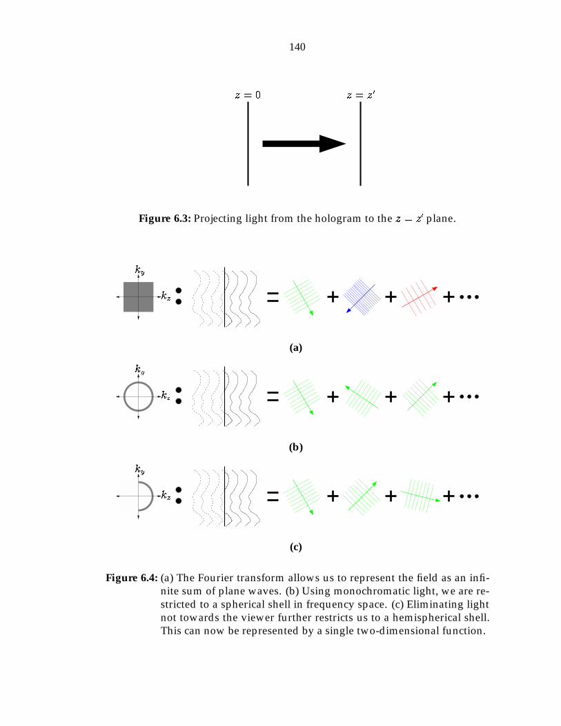
140

z = 0 z = z0

Figure 6.3: Projecting light from the hologram to the z = z0 plane.

kz

ky

(a)

kz

ky

(b)

kz

ky

(c)

Figure 6.4: (a) The Fourier transform allows us to represent the field as an infi-nite sum of plane waves. (b) Using monochromatic light, we are re-stricted to a spherical shell in frequency space. (c) Eliminating lightnot towards the viewer further restricts us to a hemispherical shell.This can now be represented by a single two-dimensional function.

141

Inverting this yields

F (~x) = F�1~k

nf(~k)

o(~x) =

ZZZf(~k)e�i(~k�~x)dkxdkydkz.(6.2)

For a fixed ~k, the expression e�i(~k�~x) describes a plane wave of wavelength 2�k

traveling in the k direction. Thus Equation (6.2) tells us that F can be treated as

a weighted sum of an infinite set of plane waves (Figure 6.4(a)).

If we limit the hologram to monochromatic light of a given wavelength �,

we eliminate all the plane waves except those for which k~kk = 2��

. This causes

f to become zero except over a spherical shell of radius 2��

centered at the origin

(Figure 6.4(b)). It can now be mapped to a pair of two-dimensional functions,

f+(kx; ky) and f�(kx; ky), which represent the light emitted over the positive z

and negative z directional hemispheres, respectively. We have

f(~k) = f+(kx; ky)�(kz � k0

z) + f�(kx; ky)�(kz + k0z),(6.3)

where k0z �r�

2��

�2� k2x � k2y.

The fact that the hologram only emits on the positive z side lets us set

f�(kx; ky) = 0, yielding

f(~k) = f+(kx; ky)�(kz � k0

z).(6.4)

The three-dimensional frequency decomposition now maps to a two-dimen-

sional function (Figure 6.4(c)).

Combining Equation (6.2) and Equation (6.4) and selecting a fixed z = z0

yields

F (x; y; z0) =ZZ

f+(kx; ky)e�ik0zz

0

e�i(kxx+kyy)dkxdky(6.5)

= F�1(kx;ky)

nf+(kx; ky)e

�ik0zz0o(x; y) .(6.6)

142

phasefactor

TransformInverseFourier

Transform

F (x; y; 0) F (x; y; z0)

f+(kx; ky) f+(kx; ky)e�ik0zz

0

Figure 6.5: Schematic representation of the process of projecting light from oneplane to another parallel plane.

Inverting this gives us

f+(kx; ky) = e+ik0zz0

F(x;y) fF (x; y; z0)g (kx; ky) ,(6.7)

which, when applied to the known field at the hologram plane, z0 = 0, becomes

f+(kx; ky) = F(x;y) fF (x; y; 0)g (kx; ky) .(6.8)

Thus, we can use Equation (6.8) to find f+ from the computed hologram, and

then apply Equation (6.6) to determine the light at any plane parallel to the

hologram This process is shown in Figure 6.5.

6.1.2 Rotation

Now suppose that we wish to find the field at a plane which is not parallel to the

hologram (Figure 6.6(a)). For any such plane, we can always find a new frame

of reference in which it is perpendicular to the z axis at some distance z0 from

the origin and in which the hologram intersects the origin (Figure 6.6(b)). This

new reference frame is separated by the original one by some rotation R.

Let us apply Equation (6.8) in the original frame of reference to obtain f+.

Recall that this two-dimensional function maps to the directional hemisphere in

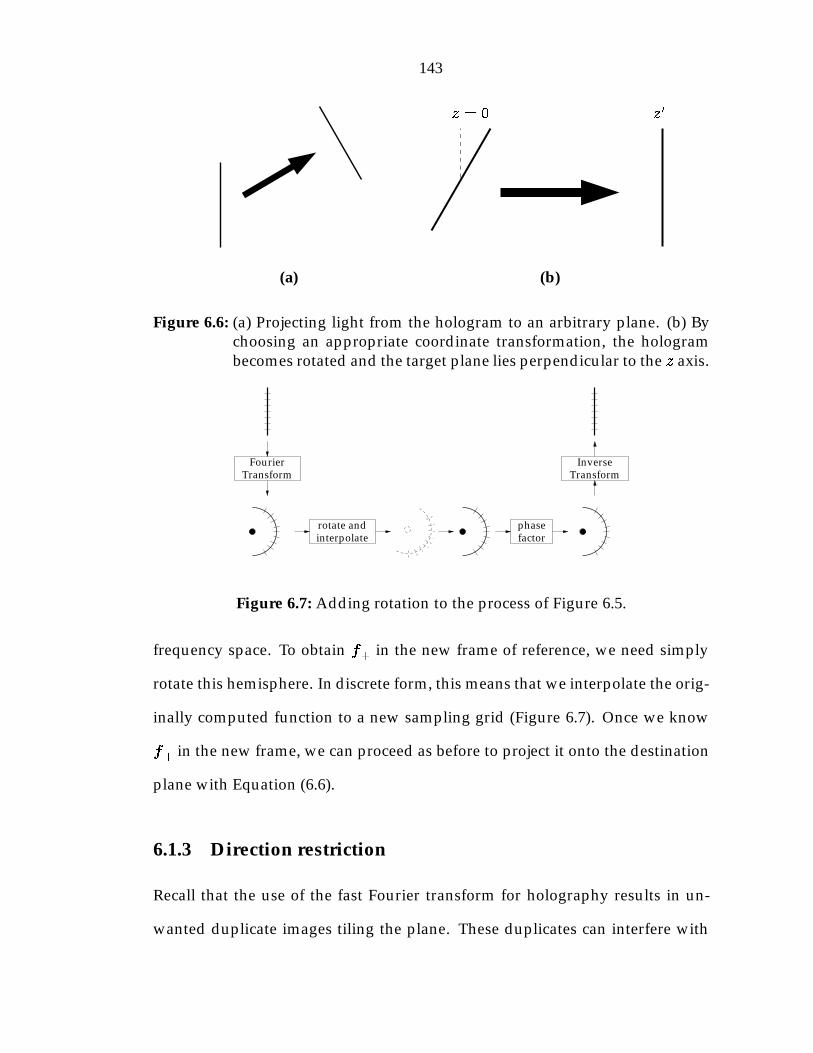
143

(a)

z = 0 z0

(b)

Figure 6.6: (a) Projecting light from the hologram to an arbitrary plane. (b) Bychoosing an appropriate coordinate transformation, the hologrambecomes rotated and the target plane lies perpendicular to the z axis.

interpolate

FourierTransform

phasefactor

TransformInverse

rotate and

Figure 6.7: Adding rotation to the process of Figure 6.5.

frequency space. To obtain f+ in the new frame of reference, we need simply

rotate this hemisphere. In discrete form, this means that we interpolate the orig-

inally computed function to a new sampling grid (Figure 6.7). Once we know

f+ in the new frame, we can proceed as before to project it onto the destination

plane with Equation (6.6).

6.1.3 Direction restriction

Recall that the use of the fast Fourier transform for holography results in un-

wanted duplicate images tiling the plane. These duplicates can interfere with

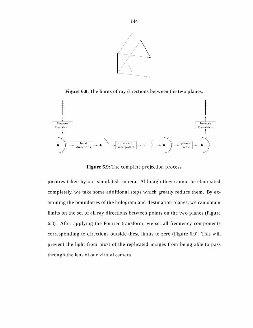
144

Figure 6.8: The limits of ray directions between the two planes.

interpolate

FourierTransform

limitdirections

phasefactor

TransformInverse

rotate and

Figure 6.9: The complete projection process

pictures taken by our simulated camera. Although they cannot be eliminated

completely, we take some additional steps which greatly reduce them. By ex-

amining the boundaries of the hologram and destination planes, we can obtain

limits on the set of all ray directions between points on the two planes (Figure

6.8). After applying the Fourier transform, we set all frequency components

corresponding to directions outside these limits to zero (Figure 6.9). This will

prevent the light from most of the replicated images from being able to pass

through the lens of our virtual camera.

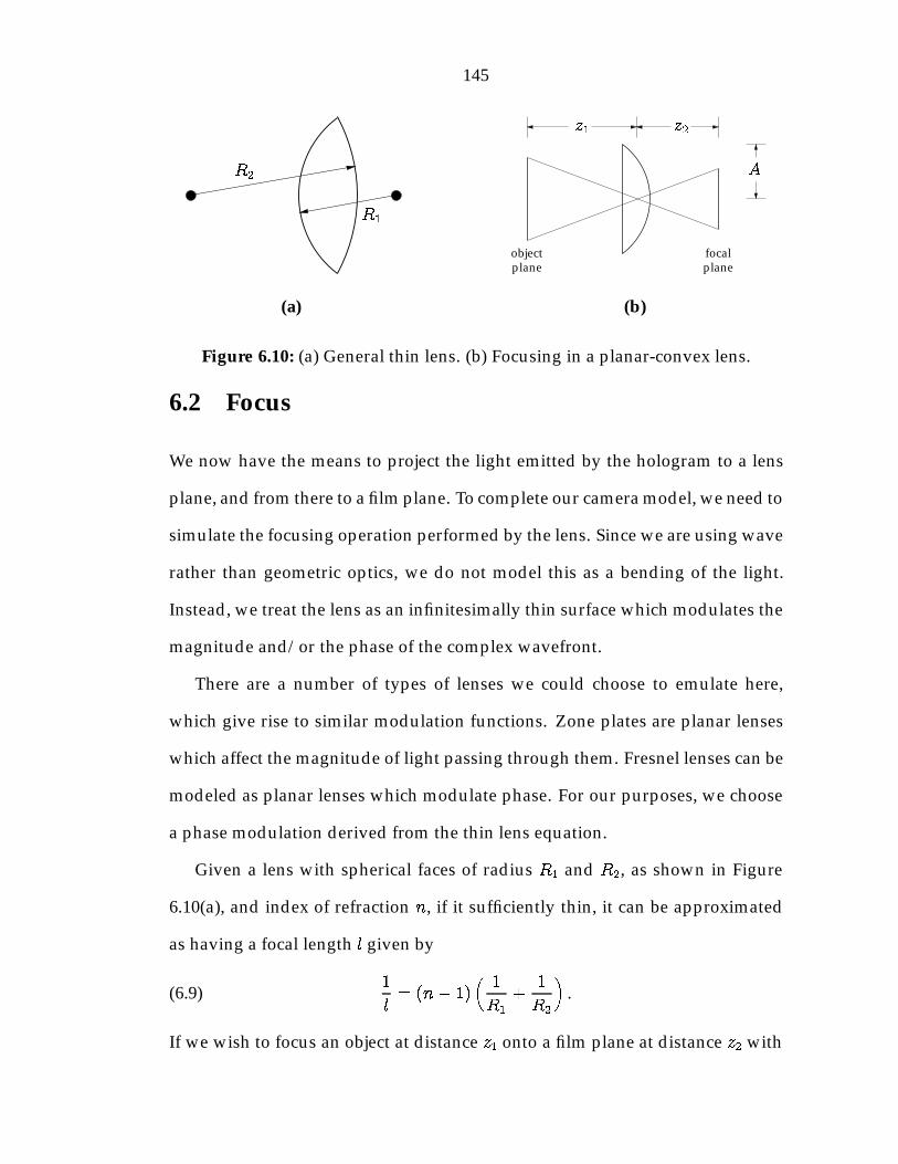
145

R1

R2

(a)

objectplane plane

focal

z1 z2

A

(b)

Figure 6.10: (a) General thin lens. (b) Focusing in a planar-convex lens.

6.2 Focus

We now have the means to project the light emitted by the hologram to a lens

plane, and from there to a film plane. To complete our camera model, we need to

simulate the focusing operation performed by the lens. Since we are using wave

rather than geometric optics, we do not model this as a bending of the light.

Instead, we treat the lens as an infinitesimally thin surface which modulates the

magnitude and/or the phase of the complex wavefront.

There are a number of types of lenses we could choose to emulate here,

which give rise to similar modulation functions. Zone plates are planar lenses

which affect the magnitude of light passing through them. Fresnel lenses can be

modeled as planar lenses which modulate phase. For our purposes, we choose

a phase modulation derived from the thin lens equation.

Given a lens with spherical faces of radius R1 and R2, as shown in Figure

6.10(a), and index of refraction n, if it sufficiently thin, it can be approximated

as having a focal length l given by

1

l= (n� 1)

�1

R1

+1

R2

�.(6.9)

If we wish to focus an object at distance z1 onto a film plane at distance z2 with

146

a planar-convex lens (R1 = 1), we require R2 = l(n � 1), where 1

l= 1

z1+ 1

z2

(Figure 6.10(b)). If the lens has a total aperture of radius A, then its thickness at

a distance a from the center is

� (a) =qR22 � a2 �

qR22 � A2 =

q(l(n� 1))2 � a2 �

q(l(n� 1))2 � A2.(6.10)

Since we are not limited to real materials, we can make the index of refrac-

tion become infinitely large. This has two effects. First, the thickness can be

approximated as

� (a) �A2 � a2

2l(n� 1).(6.11)

Second, any light ray striking the planar side of the lens will be refracted so as

to travel almost perpendicular to this plane. Combining these two facts, we see

that light striking the plane will travel a distance � (a) through the lens deter-

mined solely by the position at which it strikes the lens, and not by its incoming

direction.

Light entering a medium with index of refraction n is slowed by a factor

of 1

n. After traveling a distance � through such a medium, it will lag (n � 1)�

�

cycles behind light traveling the same distance through empty space. Thus,

as n becomes infinite, the lens becomes an infinitesimally thin surface which

introduces a phase delay of

e�i2� A2�a2

2l� .(6.12)

By applying this phase shift to the light projected onto the lens plane, we can

achieve the desired focusing effect.

147

6.3 Exposure

Finally, we must simulate the exposure of the film to produce an image. This

step is trivially easy. Based on the camera geometry and the relative distances

between the lens plane and the hologram and film planes, we determine the

portion of the film plane onto which the image of the hologram will project. We

determine the light intensities within this region by squaring the computed field

magnitudes. The sample spacing will be on the order of the wavelength of light,

so we downsample by simple averaging to obtain an image of a reasonable size.

6.4 Results

We tested our camera by computing several views of a hologram of Cornell’s

McGraw bell tower (Figure 6.11). Once again, the amount of memory available

proved to be a major limiting factor. In order to efficiently compute the required

FFTs, it is necessary to have the entire hologram in memory. This places a bound

on how large a hologram we can use. We can alleviate this problem to some

extent by running the program in parallel on multiple systems, with each one

taking responsibility for a portion of the data. However, given the resources

available to us, we were still only able to operate on holograms up to about 8

millimeters in size. Note that this limitation only affects our ability to use the

camera simulator. With the algorithm of the previous chapter, we are able to

generate significantly larger holograms.

The reason this concerns us is that the size of the hologram limits the size of

the camera aperture. If the aperture is too large, then their will be strong depth

of field effects, and much of the scene will appear blurry. If the aperture is too

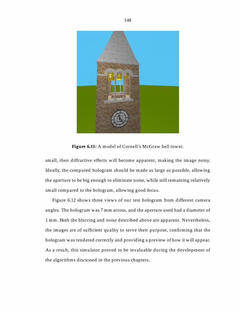
148

Figure 6.11: A model of Cornell’s McGraw bell tower.

small, then diffractive effects will become apparent, making the image noisy.

Ideally, the computed hologram should be made as large as possible, allowing

the aperture to be big enough to eliminate noise, while still remaining relatively

small compared to the hologram, allowing good focus.

Figure 6.12 shows three views of our test hologram from different camera

angles. The hologram was 7 mm across, and the aperture used had a diameter of

1 mm. Both the blurring and noise described above are apparent. Nevertheless,

the images are of sufficient quality to serve their purpose, confirming that the

hologram was rendered correctly and providing a preview of how it will appear.

As a result, this simulator proved to be invaluable during the development of

the algorithms discussed in the previous chapters.

149

Figure 6.12: Three views of the same hologram taken from different positionsusing our camera simulator.

Chapter 7

Conclusions

7.1 Summary

We have presented several tools to advance the field of computer generated

holographic stereograms.

First, we addressed the issue of compressing the enormous amount of data

required to represent the hologram down to a manageable size for transmission

and storage. We described how the JPEG compression standard can be extended

to handle the compression of lumigraphs. We also described the use of wavelet

transforms for this purpose and provide a means for encoding the transformed

data which yields compression roughly equivalent to that of the existing EZW

algorithm but in much less time. After comparing a number of wavelets, as

well as the JPEG scheme, we found the (3,3) average interpolating wavelet to

provide the best results.

Next, we described an algorithm for efficiently rendering the lumigraph. We

convert the scene geometry into a set of simple four-dimensional primitives,

and scan convert them into a set of 4D color and depth buffers. By taking ad-

150

151

vantage of coherence in all four dimensions, this method can yield tremendous

savings in computation time. Additionally, its structure is designed so as to

allow it to be implemented in hardware and serve as the basis for a real-time

holographic display system.

Finally, we presented a camera simulator to allow computed holograms to be

previewed in the absence of a real-time display. Using wave optics, we compute

the propagation of light from the hologram, through a lens, and onto the film

plane. The resulting images, while exhibiting some artifacts, allow us to assess

the correctness of our holographic rendering software.

7.2 Comments and Future Work

7.2.1 Compression

Using the best of the compression methods examined, we can obtain lumi-

graphs with only marginally perceptible error at a compression of about 2 pixels

per bit in grayscale, or 0.67 ppb for color. At first glance, this seems rather disap-

pointing. JPEG compression of 2D color images can typically achieve compres-

sion of at least 1 ppb without significant error, and we expect better performance

for a lumigraph. Several factors account for this discrepancy.

The first is that, as we discussed, memory constraints forced us to apply the

transforms to only three of the four dimensions of the lumigraph. We can expect

that with sufficient memory to transform in all four dimensions, we will obtain

higher compression.

The second factor is the difference in how our algorithm makes use of color.

Most JPEG implementations convert the image to XYZ, HSV, or some other per-

152

ceptual color space before applying the DCT. Since errors in color are signifi-

cantly less noticeable than errors in luminance, the two channels governing the

color can be compressed to a much higher degree. Only a disproportionally

small percentage of JPEG’s compression comes from the luminance channel.

On the other hand, we chose to leave the data in RGB space and compress

each channel equally. This decision was made so as to allow the computation of

the interference pattern by weighted sums, as in Equation (3.24). This form of

conversion is not compatible with any color representation other than separate

channels for each wavelength. However, for those situations where conversion

will be performed by FFT, we believe it would be well worth exploring how

much improvement could be gained by the use of an alternative color space.

The third reason for the apparent shortcoming of our algorithm is the differ-

ence in dynamic range. JPEG is normally applied to 8-bit images. Recall, how-

ever, that we chose to use lumigraphs with full floating point precision. The

scenes on which our algorithm was tested had ranges on the order of 100,000 to

1. Thus, although the number of pixels per bit that we produce is lower than

that of JPEG, the effective compression ratio is larger. Nevertheless, we feel that

there is potential here for more significant gains.

Our decision to use floating point values was motivated by a desire to take

advantage of the high dynamic range afforded by a holographic display. How-

ever, we may be preserving more information than is necessary, at the cost of

potential compression. Several recent papers on tone reproduction have de-

scribed methods for collapsing an image with a large dynamic range into a lim-

ited number of bits, while preserving important visual content. We believe that

by applying such a scheme before the wavelet transform, we should be able

153

to greatly increase the degree of compression without introducing additional

perceptual errors.

Obviously, this is, in general, contrary to our intent to maintain the original

lumigraph’s high dynamic range. However, one tone reproduction algorithm

in particular, the histogram adjustment method of Larson et.al. [59], not only

produces high quality results, but possesses the added benefit of being easily

invertible. Thus, after decompression, we can reverse the process to obtain the

original luminance values. Additionally, we are not hampered by the normal

motivation of tone reproduction, where we are mapping to some fixed num-

ber of bits determined by a particular display device. Instead we can choose

an optimal number of bits for a given lumigraph so as to provide the maxi-

mum possible compression while avoiding the loss of detail which often is an

inevitable byproduct of such algorithms.

7.2.2 Rendering

We chose to use simplices as the fundamental primitive for our renderer be-

cause their simple structure makes them very easy to represent and manipu-

late, especially for a hardware implementation. However, the repeated slicing

and subdivision used by our algorithm to perform clipping can result in the

creation of a very large number of very small simplices, reducing the efficiency.

In the theoretical worst case scenario, a single scene triangle can generate over

40,000 simplices, although this is a pathological case, and in practice we never

observed anything remotely approaching this order of magnitude.

One possible approach to help alleviate this problem is to borrow another

concept used by 2D rendering: the triangle strip. This consists of an ordered list

154

of triangles, each of which shares two vertices with the one preceding it. A trian-

gle strip requires one third the amount of data as a set of independent triangles,

and many redundant computations can be eliminated by taking advantage of

their connectivity.

We can extend this to four dimensions by creating simplex strips, each mem-

ber of which shares four of its five vertices with the simplex preceding it. The

initial simplex queue created for a polygon can always be sorted into one or two

such strips. Whenever clipping of one or more simplices in a strip results in a

new set of simplices being created, they can be inserted into the strip, sometimes

causing it to be split into two new strips. In this way, it should be possible to

perform clipping and scan conversion on an entire strip at once, thereby reduc-

ing the computational cost.

Another possible approach is to use a combination of simplices and sim-

ploids as the lowest level primitives. Like simplices, simploids also have a

structure which can be easily represented and operated on. For many of the

intermediate simploids generated by our algorithm, subdivision may not be

necessary to the performance of scan conversion. Choosing to perform this op-

eration on a simploid will undoubtedly be more complex than it would be on

a simplex, but should still provide savings over subdividing and operating on

several simplices.

7.3 Final Thoughts

Two-dimensional images are something of which we have a very strong under-

standing, as well as a great deal of experience at computing. It is therefore very

155

tempting to view a lumigraph simply as a collection of images, and to treat the

problem of computing it as a series of independent 2D renderings. However,

in so doing, we throw away a tremendous amount of coherence which can be

used to our advantage. We hope we have shown here that only by moving be-

yond two dimensions and visualizing the lumigraph as the four-dimensional

structure that it is, can we begin to produce algorithms capable of rendering

lumigraphs at the rate needed to drive a real-time holographic display.

Bibliography

[1] Robert Akka. Utilizing 6D head-tracking data for stereoscopic computergraphics perspective transformations. In Stereoscopic Displays and Applica-tions IV (Proceedings of SPIE), volume 1915, pages 147–154, 1993.

[2] Marc Antonini, Michel Barlaud, Pierre Mathieu, and Ingrid Daubechies.Image coding using the wavelet transform. IEEE Transactions on ImageProcessing, 1(2):205–220, April 1992.

[3] Stephen A. Benton. Hologram reconstructions with extended incoherentsources. Journal of the Optical Society of America, 59:1545–1546A, 1969.

[4] Stephen A. Benton. Holographic displays - a review. Optical Engineering,14(5):402–407, Sep–Oct 1975.

[5] Stephen A. Benton. Holographic displays: 1975–1980. Optical Engineering,19(5):686–690, Sep–Oct 1980.

[6] Stephen A. Benton. Display holography: An SPIE critical review of tech-nology. In Holography (Proceedings of SPIE), volume 532, pages 8–13, 1985.

[7] Stephen A. Benton, editor. Practical Holography IV (Proceedings of SPIE),volume 1212, 1990.

[8] Stephen A. Benton. Elements of holographic video imaging. In Interna-tional Symposium on Display Holography (Proceedings of SPIE), volume 1600,pages 82–95, 1991.

[9] Stephen A. Benton, editor. Practical Holography V (Proceedings of SPIE),volume 1461, 1991.

[10] Stephen A. Benton, editor. Practical Holography VI (Proceedings of SPIE),volume 1667, 1992.

[11] Stephen A. Benton, editor. Practical Holography VII: Imaging and Materials(Proceedings of SPIE), volume 1914, 1993.

156

157

[12] Stephen A. Benton. Edwin Land, 3-D, and holography. Optics and Photon-ics News, 5(10):41–43, October 1994.

[13] Stephen A. Benton, editor. Practical Holography VIII (Proceedings of SPIE),volume 2176, 1994.

[14] Stephen A. Benton, editor. Practical Holography IX (Proceedings of SPIE),volume 2406, 1995.

[15] D. J. De Bitetto. Bandwidth reduction of hologram transmission systemby elimination of vertical parallax. Applied Physics Letters, 12(5):176–178,March 1968.

[16] Jim Blinn. Jim Blinn’s Corner: A Trip Down the Graphics Pipeline. MorganKaufmann Publishers, Los Altos, CA 94022, USA, 1996. This book is acollection of columns from the journal IEEE Computer Graphics and Ap-plications.

[17] Duane K. Boman. International survey: Virtual-environment research.Computer, 28(6):57–65, June 1995.

[18] Reinhard Borner. Progress in projection of parallax-panoramagrams ontowide-angle lenticual screens. In True 3D Imaging Techniques and DisplayTechnologies (Proceedings of SPIE), volume 761, pages 35–43, 1987.

[19] E. Oran Brigham. The Fast Fourier Transform. Prentice-Hall, EnglewoodCliffs, NJ, 1974.

[20] E. Oran Brigham. The Fast Fourier Transform and Its Applications. Prentice-Hall, Englewood Cliffs, NJ, 1988.

[21] B. R. Brown and A. W. Lohmann. Complex spatial filtering with binarymasks. Applied Optics, 5(6):967–969, June 1966.

[22] Byron Brown. Improved computer-generated binary holograms. Journalof the Optical Society of America, 58:729A, 1968.

[23] C. B. Burckhardt. A simplification of lee’s method of generating holo-grams by computer. Applied Optics, 9(8):1949, August 1970.

[24] O. Bryngdahl Ch. Frere, D. Leseberg. Computer-generated holograms ofthree-dimensional objects composed of line segments. Journal of the OpticalSociety of America A, 3(5):726–730, May 1986.

[25] Hsuan Chen and F. T. S. Yu. One-step rainbow hologram. Optics Letters,2(4):85–87, April 1978.

[26] Chromatek Inc. Product literature. 11450-F North Fulton Industrial Blvd,Alpharetta, GA 30201-4703.

158

[27] D. C. Chu. Recent approaches to computer-generated holograms. OpticalEngineering, 13(3):189–195, May/June 1974.

[28] C. K. Chui. An Introduction to Wavelets. Academic Press, San Diego, 1992.

[29] C. K. Chui, editor. Wavelets: A Tutorial in Theory and Applications. Aca-demic Press, San Diego, 1992.

[30] T. E. Clifton III and Fred L. Wefer. Direct volume display devices. IEEEComputer Graphics and Applications, pages 57–65, July 1993.

[31] Patrick C. Coffield. An architecture for processing image algebra opera-tions. In Image Algebra and Morphological Image Processing III (Proceedingsof SPIE), volume 1769, pages 178–189, 1992.

[32] A. Cohen, Ingrid Daubechies, and J.-C. Feauveau. Biorthogonal basesof compactly supported wavelets. Communications on Pure and AppliedMathematics, 45:485–560, 1992.

[33] James W. Cooley and John W. Tukey. An algorithm for the machine cal-culation of complex fourier series. Mathematical Computation, 19:297–301,1965.

[34] W. J. Dallas. Computer-Generated Holograms, pages 291–366. Springer-Verlag, New York, 1980.

[35] Ingrid Daubechies. Orthonormal bases of compactly supported wavelets.Communications on Pure and Applied Mathematics, 41:909–996, November1988.

[36] Ingrid Daubechies. Ten Lectures on Wavelets. Number 61 in CBMS-NSFSeries in Applied Mathematics. SIAM, Philadelphia, 1992.

[37] Gilles Deslauriers and Serge Dubuc. Symmetric iterative interpolationprocesses. Constructive Approximation, 4:49–68, 1989.

[38] David L. Donoho. Smooth Wavelet Decompositions with Blocky CoefficientKernels. Academic Press, Inc., 1993.

[39] Jesse Eichenlaub. A novel low cost 2D/3D autostereoscopic system fornotebook computers and other portable devices. In Stereoscopic Displaysand Virtual Reality Systems II (Proceedings of SPIE), volume 2409, pages 113–117, 1995.

[40] Jesse Eichenlaub, Dan Hollands, and Jamie Hutchins. A prototype flatpanel hologram-like display that produces multiple perspective views atfull resolution. In Stereoscopic Displays and Virtual Reality Systems II (Pro-ceedings of SPIE), volume 2409, pages 102–112, 1995.

159

[41] David Ezra, Graham J. Woodgate, Basil A. Omar, Nicolas S. Holliman,Jonathan Harold, and Larry S. Shapiro. New autostereoscopic displaysystem. In Stereoscopic Displays and Virtual Reality Systems II (Proceedings ofSPIE), volume 2409, pages 31–40, 1995.

[42] D. Gabor. A new microscopic principle. Nature, 161:777–8, 1948.

[43] D. Gabor. Microscopy by reconstructed wave fronts: II. Proceedings of thePhysical Society B, 64(6):449–469, 1951.

[44] D. Gabor and Dr.-Ing. Microscopy by reconstructed wave-fronts. Proceed-ings of the Royal Society A, 197:454–487, 1949.

[45] Joseph W. Goodman. Introduction to Fourier Optics. McGraw-Hill, SanFrancisco, 1968.

[46] Steven J. Gortler, Radek Grzeszczuk, Richard Szeliski, and Michael F. Co-hen. The lumigraph. In Holly Rushmeier, editor, Computer Graphics (SIG-GRAPH ’96 Proceedings), volume 30, pages 43–54, August 1996.

[47] Paul Haeberli and Kurt Akeley. The accumulation buffer: Hardware sup-port for high-quality rendering. In Forest Baskett, editor, Computer Graph-ics (SIGGRAPH ’90 Proceedings), pages 309–318, 1990.

[48] Kenneth Haines and Debby Haines. Computer graphics for holography.IEEE Computer Graphics & Applications, pages 37–46, January 1992.

[49] Michael Halle. Multiple viewpoint rendering. In Michael F. Cohen, editor,Computer Graphics (SIGGRAPH ’98 Proceedings), pages 243–254, 1998.

[50] Andrew J. Hanson. Geometry for N-dimensional graphics. In Paul Heck-bert, editor, Graphics Gems IV, pages 149–170. Academic Press, Boston,1994.

[51] Thomas J. Haven. A liquid-crystal video stereoscope with high extinctionratios, a 28% transmission state, and one-hundred-microsecond switch-ing. In True 3D Imaging Techniques and Display Technologies (Proceedings ofSPIE), volume 761, pages 23–26, 1987.

[52] Thomas S. Huang. Digital holography. Proceedings of the IEEE, 59(9):1335–1346, September 1971.

[53] Y. Ichioka, M. Izumi, and T. Suzuki. Scanning halftone plotterand computer-generated continuous-tone hologram. Applied Optics,10(2):403–411, February 1971.

[54] Herbert E. Ives. A camera for making parallax panoramagrams. Journalof the Optical Society of America, 17:435–439, December 1928.

160

[55] Sam H. Kaplan. Theory of parallax barriers. Journal of the SMPTE,59(7):11–21, July 1952.

[56] Lloyd Kaufman. Sight and mind: an introduction to visual perception. OxfordUniversity Press, New York, 1974.

[57] M. C. King, A. M. Noll, and D. H. Berry. A new approach to computer-generated holography. Applied Optics, 9(2):471–475, February 1970.

[58] B. N. Kishto. The colour stereoscopic effect. Vision Research, 5:313–329,1965.

[59] Gregory Ward Larson, Holly Rushmeier, and Christine Piatko. A visibil-ity matching tone reproduction operator for high dynamic range scenes.IEEE Transactions on Visualization and Computer Graphics, 3(4):291–306, Oc-tober - December 1997. ISSN 1077-2626.

[60] Wai-Hon Lee. Sampled fraunhofer holograms generated by computer.Journal of the Optical Society of America, 58:729A, 1968.

[61] Wai Hon Lee. Sampled fourier transform hologram generated by com-puter. Applied Optics, 9(3):639–643, March 1970.

[62] Wai-Hon Lee. Computer generated holograms: Techniques and applica-tions. Progress in Optics, XVI(III):119–2323, 1978.

[63] Emmett N. Leith and Juris Upatnieks. Reconstructed wavefrontsand communication theory. Journal of the Optical Society of America,52(10):1123–1130, October 1962.

[64] Emmett N. Leith and Juris Upatnieks. Wavefront reconstruction withcontinuous-tone objects. Journal of the Optical Society of America,53(12):1377–1381, December 1963.

[65] Emmett N. Leith and Juris Upatnieks. Wavefront reconstruction with dif-fused illumination and three-dimensional objects. Journal of the OpticalSociety of America, 54(11):1295–1301, November 1964.

[66] D[etlef] Leseberg. Computer-generated holograms: display using one-dimensional transforms. Journal of the Optical Society of America A,3(11):1846–1851, November 1986.

[67] Detlef Leseberg. Computer generated holograms: cylindrical, conical,and helical waves. Applied Optics, 26(20):4385–4390, October 1987.

[68] Detlef Leseberg. Computer-generated holograms of 3-D objects. In Holo-graphic Optics II: Principles and Applications (Proceedings of SPIE), volume1136, pages 202–207, 1989.

161

[69] Detlef Leseberg. Computer-generated three-dimensional image holo-grams. Applied Optics, 31(2):223–229, January 1992.

[70] Detlef Leseberg and Olof Bryngdahl. Computer-generated rainbow holo-grams. Applied Optics, 23(14):2441–2447, July 1984.

[71] Detlef Leseberg and Christian Frere. Computer generated holograms of 3-D objects composed of tilted planar segments. Applied Optics, 27(14):3020–3024, July 1988.

[72] L. B. Lesem, P. M. Hirsch, and Jr. J. A. Jordan. Computer synthesis ofholograms for 3-D display. Communications of the ACM, 11(10):661–674,October 1968.

[73] L. B. Lesem, P. M. Hirsch, and Jr. J. A. Jordan. The kinoform: A newwavefront reconstruction device. IBM Journal of Research and Development,13:150–155, March 1969.

[74] Marc Levoy and Pat Hanrahan. Light field rendering. In Holly Rushmeier,editor, Computer Graphics (SIGGRAPH ’96 Proceedings), volume 30, pages31–42, August 1996.

[75] Lenny Lipton. Foundations of the Stereoscopic Cinema. Van Nostrand Rein-hold, New York, 1982. ISBN 0-442-24724-9.

[76] Lenny Lipton. Field-sequential electronic stereoscopic projector. In Projec-tion Display Technology, Sytems, and Applications (Proceedings of SPIE), vol-ume 1081, pages 94–100, 1989.

[77] Lenny Lipton. Large screen electro-stereoscopic displays. In Large-ScreenProjection Displays II (Proceedings of SPIE), volume 1255, pages 108–113,1990.

[78] Lenny Lipton. The evolution of electronic stereoscopy. SMPTE Journal,100:332–336, May 1991.

[79] Lenny Lipton and Arthur Berman. Push-pull liquid crystal modulatorfor electronic stereoscopic display. In Woodrow E. Robbins, editor, Three-Dimensional Imaging and Remote Sensing (Proceedings of SPIE), volume 902,pages 31–44, 1988.

[80] Lenny Lipton and Lhary Meyer. A flicker-free field-sequential stereo-scopic video system. SMPTE Journal, 93:1047–1051, November 1984.

[81] Charles F. Van Loan. Computational Frameworks for the Fast Fourier Trans-form. SIAM, Philadelphia, 1992.

162

[82] A. W. Lohmann and D. P. Paris. Binary fraunhofer holograms, generatedby computer. Applied Optics, 6(10):1739–1748, October 1967.

[83] Mark Lucente. Optimization of hologram computation for real-time dis-play. In Practical Holography VI (Proceedings of SPIE), volume 1667, pages32–43, 1992.

[84] Mark Lucente. Interactive computation of holograms using a look-up ta-ble. Journal of Electronic Imaging, 2(1):28–34, January 1993.

[85] Mark Lucente. Diffraction-Specific Fringe Computation for Electro-Holography. Ph.D. dissertation, MIT Department of Electrical Engineeringand Computer Science, August 1994.

[86] Mark Lucente. Computational holographic bandwidth compression. IBMSystems Journal, 35(3–4):349–365, 1996.

[87] Mark Lucente. Holographic bandwidth compression using spatial sub-sampling. Optical Engineering, 35(6):1529–37, June 1996.

[88] David F. McAllister, editor. Stereo Computer Graphics and Other True 3DTechnologies. Princeton University Press, Princeton, NJ, 1993.

[89] J. T. McCrickerd and Nicholas George. Holographics stereogram formsequential component photographs. Applied Physics Letters, 12(1):10–12,January 1968.

[90] P. W. McOwan, W. J. Hossack, and R. E. Burge. Three-dimensional stereo-scopic display using ray traced computer generated holograms. OpticsCommunications, 82(1):6–11, April 1991.

[91] John O. Merritt. Often overlooked advantages of 3-D displays. InWoodrow E. Robbins, editor, Three-Dimensional Imaging and Remote Sens-ing (Proceedings of SPIE), volume 902, pages 46–47, 1988.

[92] Kenneth Meyer, Hugh L. Applewhite, and Frank A. Biocca. A survey ofposition trackers. Presence, 1(2):173–200, Spring 1992.

[93] Doug Moore. Understanding simploids. In David Kirk, editor, GraphicsGems III, pages 250–255. Academic Press, 1992.

[94] Takanori Okoshi. Three-Dimensional Imaging Techniques. Academic Press,New York, 1976.

[95] Takanori Okoshi. Three-dimensional displays. Proc. IEEE, 68:548–564,May 1980.

[96] Robert Patterson and Robert Fox. The effect of testing method onstereoanomaly. Vision Research, 24(5):403–408, 1984.

163

[97] William B. Pennebaker and Joan L. Mitchell. JPEG Still Image Data Com-pression Standard. Van Nostrand Reinhold, New York, 1993.

[98] Eric G. Rawson. 3-D computer-generated movies using a varifocal mirror.Applied Optics, 7(8):1505–1512, August 1968.

[99] Whitman Richards. Stereopsis and stereoblindness. Experimental BrainResearch, 10:380–388, 1970.

[100] J. A. Roese and L. E. McCleary. Stereoscopic computer graphics for sim-ulation and modeling. Computer Graphics (SIGGRAPH ’79 Proceedings),13(3):41–47, August 1979.

[101] John A. Roese and Aida S. Khalafalla. Stereoscopic viewing with PLTZceramics. Ferroelectrics, 10(1-4):47–51, 1976.

[102] Peter Schroder and Wim Sweldens. Building Your Own Wavelets at Home,pages 15–87. 1996.

[103] Alfred Schwartz. Head tracking stereoscopic display. IEEE Transactions onElectronic Devices, pages 1123–1127, August 1986.

[104] Ian Sexton. Parallax barrier 3DTV. In Three-Dimensional Visualization andDisplay Technologies (Proceedings of SPIE), volume 1083, pages 84–94, 1989.

[105] Jerome M. Shapiro. Embedded image coding using zerotrees of waveletcoefficients. IEEE Transactions on Signal Processing, 41(12):3445–3462, De-cember 1993.

[106] Lawrence D. Sher. SpaceGraph, a true 3-D PC peripheral. In Three-Dimensional Imaging and Remote Sensing Imaging (Proceedings of SPIE), vol-ume 902, pages 10–16, 1988.

[107] Solomon Volumetric Imaging. Product literature. 2200 One KendallSquare, Cambridge, MA 02139.

[108] Richard Arend Steenblik. The chromostereoscopic process: a novel sin-gle image stereoscopic process. In True 3D Imaging Techniques and DisplayTechnology (Proceedings of SPIE), volume 761, pages 27–34, 1987.

[109] Stereographics Corporation. Product literature. 2171 East Francisco Blvd,San Rafael, CA 94901; http://infolane.com/infolane/stereog.

[110] Ivan E. Sutherland. The ulimate display. In Proceedings of the IFIP Congress,pages 506–508, 1965.

[111] Ivan E. Sutherland. A head-mounted three-dimensional display. In Pro-ceedings of the AFIPS Fall Joint Computer Conference, pages 757–764, 1968.

164

[112] Homer B. Tilton. Everyman’s real-time real 3-D. In Three-DimensionalVisualization and Display Technologies (Proceedings of SPIE), volume 1083,pages 76–83, 1989.

[113] Tullio Tommasi and Bruno Bianco. Spatial frequency analysis for the com-puter generated holography of 3-D objects. In Holographic Optics III: Prin-ciples and Applications (Proceedings of SPIE), volume 1507, pages 136–141,1991.

[114] Tullio Tommasi and Bruno Bianco. Computer-generated holograms oftilted planes by a spatial frequency approach. Journal of the Optical Societyof America A, 10(2):299–305, February 1993.

[115] G. Tricoles. Computer generated holograms: an historical review. AppliedOptics, 26(20):4351–4360, October 1987.

[116] J. J. Vos. The color stereoscopic effect. Vision Research, 6:105–107, 1966.

[117] Gregory K. Wallace. The JPEG still picture compression standard. Com-munications of the ACM, 34(4):30–44, April 1991.

[118] James P. Waters. Holographic image synthesis utilizing theoretical meth-ods. Applied Physics Leters, 9(11):405–407, December 1966.

[119] James P. Waters. Theoretical, holographic image synthesis. Journal of theOptical Society of America, 57:563A, 1967.

[120] James P. Waters. “general” fourier-transform method for synthesizing bi-nary holograms. Journal of the Optical Society of America, 58:729A, 1968.

[121] James P. Waters. Three-dimensional fourier-transform method for syn-thesizing binary holograms. Journal of the Optical Society of America,58(9):1284–1288, September 1968.

[122] John A. Watlington, Mark Lucente, Carlton J. Sparrell, Jr. V. Michael Bove,and Ichiro Tamitani. A hardware architecture for rapid generation ofelectro-holographic fringe patterns. In Practical Holography IX (Proceedingsof SPIE), volume 2406, pages 172–183, 1995.

[123] Charles Wheatstone. Contributions to the physiology of vision - part thefirst. On some remarkable and hitherto unobserved phenomena of binoc-ular vision. Philosophical Transactions of the Royal Society of London, pages371–394, 1938.

[124] R[odney] Don Williams. Direct volume visualization. In Proceedings ofVisualization ’92, pages 99–106, 1992.

165

[125] Rodney Don Williams and Jr. Felix Garcia. Volume visualization displays.Information Display, 5(4):8–10, April 1989.

[126] The future of holography. WIRED, 3(7):60, July 1995.

[127] Ian H. Witten, Radford M. Neal, and John G. Cleary. Arithmetic coding fordata compression. Communications of the ACM, 30(6):520–540, June 1987.

[128] Toyohiko Yatagai. Stereoscopic approach to 3-D display using computer-generated holograms. Applied Optics, 15(11):2722–2729, November 1976.