Efficient Recursive Speaker Segmentation for Unsupervised ...
227
Transcript of Efficient Recursive Speaker Segmentation for Unsupervised ...

E�cient Recursive SpeakerSegmentation for Unsupervised
Audio Editing
Thor Bundgaard Nielsen
Kongens Lyngby 2013
M.Sc.-2013-62

DTU Compute
Technical University of Denmark
Matematiktorvet, building 303B, DK-2800 Kgs. Lyngby, Denmark
Phone +45 4525 3031, Fax +45 4588 1399
www.compute.dtu.dk M.Sc.-2013-62

Summary
Today nearly everyone carries a microphone every waking moment. The worldand particularly the internet is awash with digital audio. This excess generatesdemand for tools, using machine learning algorithms, capable of organisationand interpretation. Thereby enriching audio and creating actionable Informa-tion.
This thesis tackles the problem of speaker diarisation, answering the question of"Who spoke when?", without the need for human intervention. This is achievedthrough the design of a custom algorithm that when given data, automaticallydesigns an algorithm capable of solving this problem optimally.
Initially this thesis scans the �eld of change-detection in general. A diversevariety of methods are studied, compared, contrasted, combined and improved.A subgroup of these methods are selected and optimised further through arecursive design. Beyond this, the raw audio is processed using a model of thespeech production system to generate a sequence of highly descriptive features.This process deconvolves an auditory �ngerprint from the literal informationcarried by speech.
Given data from normal conversation, between an arbitrary number of people,the generated algorithm is capable of identifying almost 19 out of 20 speakerchanges with very few false alarms. The algorithm operates 5 times fasterthan real-time on a contemporary PC and subsequently answers the "who" bycomparing the speaker turns and assigning labels.
The work carried out in this thesis is of particular practical use in the �eld ofaudio editing.

ii

Resumé
Næsten alle bærer en mikrofon hvert vågent øjeblik. Verdenen og især internet-tet er oversvømmet med digital lyd. Dette overskud genererer efterspørgsel efterværktøjer som, ved brug af maskine-lærings algoritmer, kan håndtere organise-ring og fortolkning. Derved beriges lyd og handlingsrettet information skabes.
Denne afhandling tackler spørgsmålet om "Hvem talte, hvornår?", uden behovfor menneskelig indgriben. Dette opnås gennem design af en nyskabende algo-ritme, som ved brug af data automatisk designer en algoritme i stand til at løsedette problem optimalt.
Efter en dybere gennemgang af teorien bag ændrings-detektion i sin helhed,anvendes en mangfoldig række metoder. Disse metoder bliver undersøgt i de-taljen, hvorefter de sammenlignes, kontrasteres, kombineres og forbedres. Enundergruppe af disse metoder bliver valgt og optimeres derefter ved brug af etrekursivt design. Ud over dette, er den rå lyd forarbejdet ved anvendelsen afen model for tale-produktions-systemet. Denne anvendes til at generere en se-kvens af højt beskrivende attributter, som a�older et auditivt �ngeraftryk fraden bogstavelige informationen båret af talen.
Givet data fra normale samtaler, mellem et vilkårligt antal mennesker, er dengenererede algoritme i stand til at identi�cere næsten 19 ud af 20 taler-skift.Disse identi�ceres med meget få falske alarmer og algoritmen operere 5 gan-ge hurtigere end realtid på en moderne PC. Derefter besvares "hvem" ved atsammenligne udsagn og tildele etiketter.
Metoder udviklet i denne afhandling er af særlig praktisk anvendelse inden forlydredigering.

iv

Preface
This Master's thesis was carried out at the department of Applied Mathemat-ics and Computer Science in collaboration with the department of ElectricalEngineering at the Technical University of Denmark, DTU. It is presented inful�lment of the requirements for acquiring an M.Sc. in Engineering Acoustics.This thesis was prepared in the period from February 2013 to June 2013, underthe supervision of Professor Lars Kai Hansen and Postdoc Bjørn Sand Jensen.
This thesis deals with the extraction of structure and information from speechcontaining multiple speakers. This is done through the extensive use and devel-opment of various machine learning methods, as well as the modelling of audiospeci�c features in the cepstral domain.
This thesis is funded by CoSound � A Cognitive Systems Approach to Enrichedand Actionable Information from Audio Streams [20].
Lyngby, 15-June-2013
Thor Bundgaard Nielsen

vi

Acknowledgements
I would like to thank my supervisor Lars Kai Hansen, whose great course onNon-Linear Signal Processing inspired this thesis, for the insightful discussionsalong the way and for helping me through the mathematical deductions. Myteacher Morten Mørup for introducing me to the topic of machine learningwhich very nearly escaped my notice. CoSound for sponsoring my ticket toDigital Audio � Challenges and Possibilities, event in Copenhagen on June 212013. My co-supervisor Bjørn Sand Jensen, particularly for helping me accessthe IMM cluster. The Acoustic Technology group for their support. Finally, forthe extensive work of proofreading the thesis, I would like to thank my brotherEmil and my father Ove for a diligent e�ort. Thanks to my family, this thesishas become much more pleasant to read.

viii

Abstract
The problem of unsupervised retrospective speaker change detection contin-ues to be a challenging research problem with signi�cant impacts on automaticspeech recognition and spoken document retrieval performance. The aim here isto design a much faster than real-time speaker diarisation software suite possi-bly for use in news audio editing. This thesis aims broadly, comparing a varietyof well-known speaker segmentation methods based around vector quantizationand Gaussian processes. These well established methods are compared to a novelstatistical change-point detection algorithm based on non-parametric divergenceestimation in the �eld of relative density-ratio estimation using importance �t-ting. All methods are optimized using a direct search method, initialized by acustom multi-step grid-search, in a recursive speaker change detection paradigm,built on Mel-Frequency Cepstral Coe�cients. Methods are compared on the ba-sis of their performance and their e�ciency on the ELSDSR speech data corpus.It is found that an inexpensive Gaussian process based on the Kullback-Leiblerdistance when optimized in this recursive SCD paradigm, can compete in termsof performance with far more expensive methods while maintaining a very highe�ciency. Further a recursive speaker change detection paradigm yields promis-ing results. Beyond this, it is shown that a simple feature selection based ona theoretical model of the human speech production system yields a markedimprovement in performance. Lastly this method is experimentally applied inthe �eld of agglomerative hierarchical speaker clustering and compared to amore well established method based on the Baysian Information Criteria. Herea novel approach similar to the Kullback-Leibler distance called the Informationchange rate shows promising results. The system developed in this thesis couldbe implemented in digital audio workstations to greatly simplify the process ofspeaker segmentation by automatically answering the question of "Who spokewhen?".

x

Contents
Summary i
Resumé iii
Preface v
Acknowledgements vii
Abstract ix
Nomenclature xv
1 Introduction 1
1.1 Speaker Change Detection . . . . . . . . . . . . . . . . . . . . . . 21.1.1 Real-time detection vs. retrospective detection . . . . . . 21.1.2 Supervised vs. unsupervised methods . . . . . . . . . . . 21.1.3 Precision in time vs. false positive rate . . . . . . . . . . . 51.1.4 Speaker change detection methods . . . . . . . . . . . . . 51.1.5 Overlapping speech . . . . . . . . . . . . . . . . . . . . . . 61.1.6 Speaker segment clustering . . . . . . . . . . . . . . . . . 6
1.2 Toolboxes and other software packages . . . . . . . . . . . . . . . 71.3 System overview . . . . . . . . . . . . . . . . . . . . . . . . . . . 7
2 Data pre-processing 11
2.1 Data . . . . . . . . . . . . . . . . . . . . . . . . . . . . . . . . . . 122.1.1 Synthetic data . . . . . . . . . . . . . . . . . . . . . . . . 132.1.2 ELSDSR speech corpus . . . . . . . . . . . . . . . . . . . 132.1.3 Splicing speech samples . . . . . . . . . . . . . . . . . . . 142.1.4 Speech sample sizes . . . . . . . . . . . . . . . . . . . . . 22

xii CONTENTS
2.1.5 Data bootstrap aggregation . . . . . . . . . . . . . . . . . 242.2 Feature extraction . . . . . . . . . . . . . . . . . . . . . . . . . . 24
2.2.1 Feature type selection . . . . . . . . . . . . . . . . . . . . 252.2.2 MFCC attributes . . . . . . . . . . . . . . . . . . . . . . . 262.2.3 MFCCs and noise . . . . . . . . . . . . . . . . . . . . . . 282.2.4 MFCC theory . . . . . . . . . . . . . . . . . . . . . . . . . 28
2.3 Change-point detection . . . . . . . . . . . . . . . . . . . . . . . 352.4 False Alarm Compensation . . . . . . . . . . . . . . . . . . . . . 35
2.4.1 Hybrid method . . . . . . . . . . . . . . . . . . . . . . . . 37
3 Methodology 39
3.1 Metric introduction . . . . . . . . . . . . . . . . . . . . . . . . . . 393.2 Speaker dissimilarity metrics . . . . . . . . . . . . . . . . . . . . 40
3.2.1 Vector Quantization . . . . . . . . . . . . . . . . . . . . . 423.2.2 Gaussian based approaches . . . . . . . . . . . . . . . . . 483.2.3 Relative Density Ratio Estimation . . . . . . . . . . . . . 52
3.3 Parameter optimisation techniques . . . . . . . . . . . . . . . . . 593.3.1 Basic grid search approach . . . . . . . . . . . . . . . . . 603.3.2 Novel method design . . . . . . . . . . . . . . . . . . . . . 613.3.3 Location of grid boundaries . . . . . . . . . . . . . . . . . 613.3.4 The Nelder-Mead method . . . . . . . . . . . . . . . . . . 623.3.5 Repeatability . . . . . . . . . . . . . . . . . . . . . . . . . 63
3.4 Miscellaneous . . . . . . . . . . . . . . . . . . . . . . . . . . . . . 683.4.1 F-measure and the confusion matrix . . . . . . . . . . . . 683.4.2 Standard Error of the Mean . . . . . . . . . . . . . . . . . 71
4 Application 73
4.1 Feature selection and method comparison . . . . . . . . . . . . . 744.1.1 Pre-training method comparison . . . . . . . . . . . . . . 744.1.2 Method training results . . . . . . . . . . . . . . . . . . . 854.1.3 Post-test method comparison . . . . . . . . . . . . . . . . 96
4.2 Method comparison conclusion . . . . . . . . . . . . . . . . . . . 1044.3 Method re�nement . . . . . . . . . . . . . . . . . . . . . . . . . . 105
4.3.1 Backwards feature selection . . . . . . . . . . . . . . . . . 1054.3.2 Training results . . . . . . . . . . . . . . . . . . . . . . . . 1064.3.3 Test results . . . . . . . . . . . . . . . . . . . . . . . . . . 110
4.4 Method re�nement conclusion . . . . . . . . . . . . . . . . . . . . 114
5 Further work 115
5.1 Speaker clustering . . . . . . . . . . . . . . . . . . . . . . . . . . 1155.1.1 Agglomerative Hierarchical Clustering . . . . . . . . . . . 1165.1.2 AHC: Dissimilarity metrics . . . . . . . . . . . . . . . . . 117
5.2 Recursive False Alarm Compensation . . . . . . . . . . . . . . . . 1235.3 Mimicking news pod-cast data . . . . . . . . . . . . . . . . . . . 127

CONTENTS xiii
5.4 Promising avenues . . . . . . . . . . . . . . . . . . . . . . . . . . 129
6 Final conclusions 131
A MATLAB Code 135
A.1 Main Scripts . . . . . . . . . . . . . . . . . . . . . . . . . . . . . 135A.1.1 Main: Speaker Change Detection . . . . . . . . . . . . . . 135A.1.2 Main: Speaker Clustering . . . . . . . . . . . . . . . . . . 139
A.2 Parameter Optimisation . . . . . . . . . . . . . . . . . . . . . . . 144A.2.1 Main: Parameter Optimisation . . . . . . . . . . . . . . . 144A.2.2 Objective Function . . . . . . . . . . . . . . . . . . . . . . 147A.2.3 Parameter Optimisation . . . . . . . . . . . . . . . . . . . 147
A.3 SCD Methods . . . . . . . . . . . . . . . . . . . . . . . . . . . . . 149A.3.1 Main: Gaussian approach section . . . . . . . . . . . . . . 149A.3.2 Kullback Leibler distance . . . . . . . . . . . . . . . . . . 150A.3.3 Divergence Shape Distance . . . . . . . . . . . . . . . . . 151A.3.4 Main: Vector Quantization section . . . . . . . . . . . . . 151A.3.5 Vector Quantization Distortion . . . . . . . . . . . . . . . 152A.3.6 Main: Relative Density Ratio Estimation . . . . . . . . . 153A.3.7 Change Detectoion front-end for RuLSIF . . . . . . . . . 154A.3.8 RuLSIF . . . . . . . . . . . . . . . . . . . . . . . . . . . . 155
A.4 False Alarm Compensation . . . . . . . . . . . . . . . . . . . . . 157A.4.1 Main: False Alarm Compensation section . . . . . . . . . 157A.4.2 False Alarm Compensation . . . . . . . . . . . . . . . . . 159A.4.3 FAC Performance . . . . . . . . . . . . . . . . . . . . . . 162
A.5 Data Handling . . . . . . . . . . . . . . . . . . . . . . . . . . . . 164A.5.1 ELSDSR front-end for Data Splicing . . . . . . . . . . . . 164A.5.2 Data Splicing . . . . . . . . . . . . . . . . . . . . . . . . . 166A.5.3 Main: Feature Extraction section . . . . . . . . . . . . . . 168A.5.4 Modi�ed version of ISP's MFCC Extraction . . . . . . . . 169A.5.5 Main: MFCC segmentation section . . . . . . . . . . . . . 186A.5.6 MFCC segmentation . . . . . . . . . . . . . . . . . . . . . 187A.5.7 Main: Metric Peak Detection section . . . . . . . . . . . . 187A.5.8 Metric Peak Detection . . . . . . . . . . . . . . . . . . . . 187
A.6 Miscellaneous . . . . . . . . . . . . . . . . . . . . . . . . . . . . . 188A.6.1 F-measure . . . . . . . . . . . . . . . . . . . . . . . . . . . 191A.6.2 SCD Main Wrapper . . . . . . . . . . . . . . . . . . . . . 191A.6.3 Principal Component Analysis . . . . . . . . . . . . . . . 192A.6.4 Receiver Operator Characteristics . . . . . . . . . . . . . 192A.6.5 Welch's t-test . . . . . . . . . . . . . . . . . . . . . . . . . 194
Bibliography 195

xiv CONTENTS

Nomenclature
Symbols
Greek
αcd Mcd gainαF F-measure weightαFAC MFAC gainαR Mixture-density
Γ Gamma function
δ(x) Error term
θ(n) Impulse responseΘ(k) Spectral impulse response
λ Regularization parameter (RuLSIF)
µ Population meanµk Centroid position of cluster k
σ Width of kernel K(xA;xB)Σ Population covariance matrix
υ D.o.F

xvi Nomenclature
Roman
An Preceding analysis window at time tn
Bn Succeeding analysis window at time tn
cθ(k) Cepstral impulse responsece(n) Cepstral excitation sequenceck (k = 1, 2, . . . ,K) kth code-vector (cluster)cs(n) Cepstral speech signalCθ(k) Spectral magnitude of impulse responseCA Codebook for ACB Codebook for BCe(k) Spectral magnitude of excitation sequenceCn The nth MFCC
D Number of dimensions
e(n) Excitation sequenceE(k) Spectral excitation sequence
f Frequency (independent variable of spectrum)fmel Mel-frequency scale independent variablef(y) Taylor expansionfn False negativesfp False positivesF F-measureFCDF Student's t CDF
g(x|θ) (θ = θ1, θ2, . . . , θN )T Density-ratio with parameters θ
H0 Null hypothesis
K K-means codebook sizeK(xA;xB) Gaussian kernelKmel Mel �lter bank sizeKLdivergence Kullback-Leibler divergenceKLdistance and KL Kullback-Leibler distance

xvii
law Analysis window lengthls Analysis window Shift length
Mcd Moving average threshold of change-detection algorithmMFAC Moving average threshold of FAC algorithm
N Sample sizeN Gaussian (normal) distribution
p Probabilityp(x) Example PDFP Independent parameters needed for full descriptionPA(x) A population PDFPB(x) B population PDFPRC Precision
q(x) Example PDFqjk Entries of QQ Sample covariance matrix (estimate of Σ)
rα Alpha-relative density-ratioRCL RecallRlen A random length drawn from a uniform distribution between
a �xed lower and upper boundary.Rsample A random speech sample drawn from the pool of samples
longer than Rlenrnk Vector signifying to which cluster xn belongs
s Estimate of population standard deviations(n) Speech signalS(k) Spectral speech signalSk (k = 1, 2, . . . ,Kmel) Outputs of the Mel �lter bank
±t95% The t-scores at the edges of the con�dence intervaltn True negativestn nth potential change-point's temporal positiontp True positivest-score The ratio of the departure of an estimated parameter from
its notional value and its standard errorTi Change-point width, another change-point must be at least
±Ti2 awayTmax De�nes the largest amount of data in all algorithms

xviii Nomenclature
X = {x1, x2, . . . , xN} Feature vector sequenceX Sample mean (estimate of µ)
Z Standard score of a raw score X
Glossary
AGGM Adapted Gaussian Mixture ModelAHC Agglomerative Hierarchical ClusteringAUC Area Under the Curve
BIC Bayesian Information Criterion
CDF Cumulative Distribution FunctionCMFAC Combined Metric False Alarm CompensationCMS Cepstral Mean SubtractionCPU Central Processing Unit
DAW Digital Audio WorkstationDCT Discreet Cosine TransformDFT Discrete Fourier TransformD.o.F Degrees of FreedomDTU Technical University of Denmark
ELSDSR English Language Speech Database for Speaker RecognitionEM-algorithm Expectation-Maximization algorithm
FAC False Alarm CompensationFFT Fast Fourier TransformFSCL Frequency-Sensitive Competitive Learning
GMM Gaussian Mixture Model
HMM Hidden Markov Model
ICA Independent Component AnalysisICR Information Change RateIDFT Inverse Discrete Fourier Transformi.i.d independent and identically distributed

xix
IMM Department of Mathematical Modelling (at DTU)ISP Intelligent Sound Processing toolbox
JIT Just-In Time (accelerator)
KL Kullback-Leibler distanceKL (FULL) Kullback-Leibler distance using full Mel-rangeKL (lower) Kullback-Leibler distance using lower Mel-rangeKL (upper) Kullback-Leibler distance using upper Mel-rangeKLEIP Kullback-Leibler Importance Estimation ProcedureK-means K-means clustering
LBG Linde-Buzo-Gray algorithmLOF Local Outlier FactorLSPs Line Spectrum PairsLTI Linear Time-Invariant (LTI-system)
MATLAB MATrix LABoratoryMel The Mel scaleMFC Mel-Frequency CepstrumMFCC Mel-Frequency Cepstral Coe�cientMLLR Maximum Likelihood Linear Regression
PCA Principal Component AnalysisPDF Probability Density FunctionPE Pearson divergencePLP Perceptual Linear PredictionPRC Precision (a constituent of the F-measure)
Q.E.D. Quod Erat Demonstrandum "Which had to be demonstrated"
RCL Recall (a constituent of the F-measure)RFAC Recursive False Alarm CompensationROC Receiver Operating Characteristic (curve)RuLSIF Relative unconstrained Least-Squares Importance Fitting
SEM Standard Error of the MeanSCD Speaker Change DetectionSDR Spoken Document RetrievalSNR Signal-to-Noise RatioSOM Self Organizing MapsSTE Short-Time EnergySTFT Short-Time Fourier Transform

xx
TIMIT Acoustic-Phonetic Continuous Speech Corpus
uLSIF unconstrained Least-Squares Importance Fitting
VQ Vector QuantizationVQD Vector Quantization Distortion
WCSS Within-Cluster Sum of SquaresWTA Winner-Takes-All (in the context of K-means)
ZCR Zero-Crossing Rate

Chapter 1
Introduction
The internet has become a vast resource for news pod-casts and other mediacontaining primarily speech. This poses an interesting problem as traditionaltext-based search engines will only locate such content through informationtagged onto the audio-�les manually. Manual labelling of audio content is anextensive task and therefore necessitates automation. This in turn created thewhole �eld of Speaker Change Detection, SCD, or speaker diarisation, involvingmethods from machine learning and pattern recognition.
This thesis will explore a range of available methods for SCD and comparethem for use in audio editing. Audio editing involves a rather tedious processof familiarisation with the individual segments of the media content. The hopeis that the aforementioned methods can ease and simplify this process, thusempowering Digital Audio Workstations, DAWs, by adding automated speakerdiarisation.
Optimally a DAW using speaker diarisation would be able to search inside au-dio �les for high level information, here referring to topics, speakers, environ-ments, etc. This thesis will however focus primarily on SCD, as it builds onthe knowledge gathered from the creation of Castsearch [87], a context basedSpoken Document Retrieval, SDR, search engine. During the creation of Cast-search, Jørgensen et al. designed a system for audio classi�cation [55]. Thisclassi�cation system includes the classes; Speech, music, noise and silence. This

2 Introduction
classi�cation system was applied to allow raw data to be processed, the use ofsuch a system in this thesis is discussed in section 2.1. To clarify this thesis willfocus solely on audio content. In other words incorporation of audio meta-data,audio transcriptions, associated video content, etc., is outside the scope of thisthesis.
1.1 Speaker Change Detection
SCD is the process of locating the speaker to speaker changes in an audio stream.This section will delineate the methods found in the �eld of SCD and describetheir general application is this thesis. This section will also brie�y touch onspeaker clustering, a process which SCD enables.
The end goal is to hypothesize a set of speaker change-points by comparingsamples before and after a potential change-point at regular intervals, see �gure1.1.
1.1.1 Real-time detection vs. retrospective detection
The process of detecting abrupt changes in an audio stream must be dividedinto two distinct sub-�elds with disparate challenges and trade-o�s involved.As the title suggests these sub-�elds revolve around the proximity to real-timedetection. As will be mentioned below the metric-based methods employedin this thesis require a certain amount of data after a potential change pointin order to detect it. In addition to the requirements on data, there are therequirements on processing time. The aim of this thesis is to design a systemthat takes recordings, thus not real-time, and process these. This processingmust however be comparable or preferably much quicker than real-time in orderto retain its usefulness. The work here will therefore use optimised retrospectivedetection.
1.1.2 Supervised vs. unsupervised methods
Another way to bisect the �eld of SCD is a division into supervised and unsuper-vised methods. If the number of speakers and identities are known in advance,supervised models for each speaker can be trained, and the audio stream can

1.1 Speaker Change Detection 3
Figure 1.1: This �gure is presented as a rough reference of the basic concept:Which is to compare segments of data before and after a potentialchange-point and judge whether it is di�erent enough. The data,consist of a sequences of feature vectors describing the sound overa small interval. As seen the �gure uses a variety of parameters,which will be described throughout this thesis as they becomerelevant, these include the analysis windows A and B, of lengthlaw, as they are shifted forward in time. This occurs by regularincrements of ls, to the next potential change-point at time tn.The reader is encouraged to review this �gure at regular intervals.It should be noted that the proportions portrayed in this �gureare greatly exaggerated.

4 Introduction
Figure 1.2: Rationale of direct density-ratio estimation. As seen a shortcutto the standard approach is taken. Rather than model the priorand the posterior data individually only to subsequently estimatethe ratio, a more direct method is to directly model the ratio, seesecion 3.2.3. Figure concept borrowed from [75].
be classi�ed accordingly. If the identities of the speakers are not known in ad-vance unsupervised methods must be employed. Due to the nature of the data;unsupervised SCD is a premise of this thesis and its approaches can roughlybe divided into three classes, namely energy-based, metric-based and directdensity-ratio estimation:
Energy-based methods rely on thresholds in the audio signal energy. Changesare found at silence-periods. In broadcast news the audio production can bequite aggressive, with only little if any silence between speakers, which makesthis approach less attractive. Whereas metric-based methods basically modelthe data before and after a potential change point and subsequently measuresthe di�erence between these consecutive frames that are shifted along the audiosignal.
Despite the established results of these metric based methods, they have a dis-advantage; they try to estimate a distinct Probability Density Functions, PDFs,before and after a potential change point, rather than directly estimating thedi�erence between these. Since this di�erence contains all required information,the intermediate step of gathering information only to discard it later is circum-vented, see 1.2. This group of methods is called direct density-ratio estimationand is a fairly new idea in the �eld of SCD; with the method, RuLSIF [75],applied here designed some months ago, see section 3.2.3.

1.1 Speaker Change Detection 5
1.1.3 Precision in time vs. false positive rate
The process of SCD has an inbuilt trade-o� that needs to be addressed. Inorder to detect short speaker segments it needs to be fairly constrained in time.This however leads to a smaller dataset per possible change point and naturallycauses a higher amount of false positives. Turning SCD into an iterative processcan mediate this trade-o� between the ability to notice short segments vs. ahigher false positive rate. This method has previously been called false alarmcompensation, is applied in this thesis and is described in section 2.4.
1.1.4 Speaker change detection methods
Speaker change detection methods used in this project can be further groupedinto three subgroups:
1. Gaussian Processes
2. Vector quantization
3. Direct density-ratio estimation
The �rst subgroup are the distance measures between separate multivariateGaussians trained on data before and after the potential change-point. Theseinclude the Kullback-Leibler Distance, here termed KLdistance or simply KL,and a simpli�cation of it, the so-called Divergence Shape Distance, DSD, whichfocuses solely on locating covariance changes. For more details see section 3.2.2.
The second subgroup is the Vector Quantization, VQ, approach which incorpo-rates a variety of approaches to 'discover' the underlying structure of a datasetthrough iteratively improved guesses. These guesses are in the form of a muchsmaller amount of representative data, the di�erence is then measured in the to-tal movement of this representative data, called Vector Quantization Distortion,VQD. For more details see section 3.2.1.
Lastly, for the Direct density-ratio estimation a variant of Kullback-Leibler Im-portance Estimation Procedure, KLEIP, called Relative unconstrained Least-Squares Importance Fitting, RuLSIF, introduced by Liu et al. [75] is applied.The concept behind this method is slightly more abstract, but revolves aroundmodelling the distortion of the prior data required to produce the posteriordata and then condensing this distortion model into a single number. KLIEP

6 Introduction
is designed to be coordinate transformation invariant, this however has the dis-advantage of an increased sensitivity to outliers. For this reason the variant,RuLSIF, is preferable in practical use. For more details see section 3.2.3.
All methods are metric-based; in essence this means that they supply a numberfor every point in time. The magnitude of this number is correlated with thelikelihood of a change-point at that moment. These metrics therefore needto be thresholded to yield de�nite predictions, rather than a smooth scale ofpossibilities. These thresholds will be de�ned relative to a smoothed version ofthe metric itself, see �gure 1.1. For more details see section 1.1 and 2.4
1.1.5 Overlapping speech
Since real dialogue does not always conform to the simple model of speaker turnsthe possibility of overlapping speech segments is a liability and the de�nitionfor 'babble noise' is vague in this sense. Overlapping speech naturally spreads aspeaker change over time, this may even blur the speaker change to insigni�canceand a smooth transition to a di�erent speaker altogether is a real liability. Themethods discussed in section 1.1.3 can alleviate this issue assuming the notionof speaker turns remains valid. This issue naturally lowers the precision of themodel, in a sense this issue will be regarded as a single speaker in speech noise.The data used in this thesis does not contain overlapping speech; therefore itsimagined consequences are purely theoretical.
1.1.6 Speaker segment clustering
Once a dialogue has been separated into speaker turn segments, these segmentscan be clustered. This process will produce a reasonable guess as to the amountof speakers present in the dialogue and a notion of �who said what when�. Theamount of background noise and other such limitations may impact the perfor-mance of this step.
In this thesis several approaches to speaker clustering within the �eld of Al-gomerative Hierarchical Clustering [8], AHC, have been compared; the generalconcept is to start by assuming that every speaker turn is a unique person. Thealgorithm then iteratively combines the most similar segment until only 2 seg-ments remain. The correct amount of speakers is then found by looking for thecombination where the constituents were the most dissimilar.
AHC naturally requires a metric by which to judge the dissimilarity between

1.2 Toolboxes and other software packages 7
speakers. Here the tested metrics include all the metric described in section3.2 along with a Bayesian Information Criterion, BIC, approach and a furtherimprovement on this termed Information Change Rate, ICR, [42].
Unfortunately speaker clustering was started late in the thesis, as SCD naturallyis a prior step. The scarcity of available computing resources at that pointwas enhanced by unforeseen circumstances, see section 4.3.1. This necessarilydeprioritised a rigorous approach to speaker clustering. The relevant softwarewas written, see appendix A.1.2, but were only lightly experimented with in thefurther work section 5.
This step could have an important role to play as information gathered herecould have hinted at which segments contain missed change points and mighthave facilitated the possibility of the software storing a pro�le for a particularspeaker for later recognition.
1.2 Toolboxes and other software packages
All software is developed using MATLAB and its accompanying toolboxes. Inaddition to this, custom toolboxes were employed including; the IntelligentSound Processing, ISP, Toolbox, developed as part of the Intelligent Soundproject by Jensen et al. [53] and Mike Brookes' VOICEBOX toolbox [13]. Itshould be mentioned that the ISP toolbox has been adapted to support a 64 bitwindows based OS, along with a number of technical improvements, wheneverunsupported features were required, see section 4.3.1.
1.3 System overview
This section presents a basic modular design of the proposed system given as a�ow chart in �gure 1.3. The process starts with a raw audio sample containingspeech, with multiple speakers. This raw data is far too redundant and messyto reliably determine speaker changes. The raw data is therefore fed into apreprocessing mechanism that generates the raw audio feature, the MFCCs, seesection 2.2.
The system subsequently blindly segments these MFCCs into 3 second segment,with a new segment starting every 0.1 seconds, marking a position to be checkedfor a possible change-point. This results in an organised data structure, see�gure 1.1.

8 Introduction
Figure 1.3: Simpli�ed overview of the system developed in this thesis pre-sented as a one-way �ow chart, where arrows mark the outputsand inputs of the various modules. Section 1.3 is dedicated todescribing this �gure in detail.

1.3 System overview 9
Prior to checking the possible speaker change points, it is veri�ed that all thesesegments contain primarily speech. Segments containing music, silence or clas-si�ed as other are discarded.
All segments containing primarily speech are then fed into the speaker changedetection module. This module, using only the 3 second segment before andafter a possible change-point quickly sorts through the vast majority change-points.
The remaining possible change-points are then scrutinised using as much dataas possible by the false alarm compensation module, which attempts to identifyand remove the remaining false positives. This process concludes with a set ofhypothesized speaker change points and the corresponding speaker turns.
The speaker turns are then handed to an unsupervised clustering module whichassigns a label to each speaker and subsequently marks every speaker turns withthe label of its speaker, using an agglomerative hierarchical clustering approach.

10 Introduction

Chapter 2
Data pre-processing
This chapter will begin with a description of the available data corpora, whyELSDSR was selected in lieu of more common choices, and why raw news pod-cast data was not applied. Given this information the methods involved inapplying the selected data will be explained, and a deeper analysis is conductedinto potential weak links of the process.
The chapter will then proceed to an exhaustive search of the commonly usedfeature extraction techniques applied in SCD and related �elds, speaker recog-nition, speaker diarisation, etc. The process concludes with the selection ofMel-Frequency Cepstral Coe�cients, MFCCs, as the sole features used in thisthesis.
This is followed by a thorough description of the theory, the methods, the rea-sons and the attributes of the MFCCs. This process concludes with a range ofpossible feature sets; these feature sets are compared in section 4.1.
Finally, this chapter will conclude with a description of the methodologies andpractices applied to detect speaker changes and to reject false speaker changes.This �nal part is accompanied by the theory and concepts behind a novel hybridapproach based on combining unrelated SCD methodologies.

12 Data pre-processing
2.1 Data
A dataset of speech changes is required in order to train, test and compare thespeaker change detection and speaker clustering methods. In addition to this adata set is needed to evaluate hyper parameters and �nally a dataset is neededto evaluate the performance of the full system.
As the present work builds the preliminary work for CastSearch, by Mølgaard etal. [87], and is intended for use in news editing; it seems natural to acquire theCNN (Cable News Network) pod-cast dataset. This dataset presently consists of1913 pod-cast, totalling about 6.6GB. Due to the size alone the dataset containsmore than enough speaker variety and speaker changes.
The use of the CNN data does however pose some problems. Firstly since it ismerely recordings of actual news shows it contains a mixture of speech, music,silence and other. All non-speech section would have to be �ltered out, sincethis project is focused on detecting changes from one speaker to another, notfrom speaker to music, etc.
However even with the data preprocessed to only include speech a signi�cantproblem remains, namely the quality of the di�erent speech segments. Newsanchors usually have expensive equipment and are situated in studios. Whereaswith reporters in the �eld, background noise, bandwidth and bit-rates play alarge role in the quality of the recording.
These are powerful cues as they almost always signify actual speaker changes.They are however not cues speci�c to the speaker and are therefore not actualcues at all, but merely a potentially powerful masking of cues correlated withactual cues. In addition they represent a loss of information and can thereforenot be corrected for or �ltered away.
And �nally the CNN data is not annotated, requiring a tedious process of manuallabelling, not always possible since the assumption of individual speaker turnsdoes not always fully apply. All in all using actual raw data may hinder ratherthan serve the purpose of training a speaker change detection model. As suchthe only alternative is to design synthetic data that comes as close to the realdata as possible, without the inherent problems mentioned above.

2.1 Data 13
2.1.1 Synthetic data
Since the use of raw data for model training is not viable, the use of syntheticdata is necessary. Several options, corpora, are readily available for this pur-pose. They are however generally accompanied by a rather large price tag. Thedepartment DTU Compute has two usable corpora on hand, the ELSDSR [31]and the TIMIT [37] corpora.
Since the ELSDSR corpus contains a su�cient amount of data and has longuninterrupted speaker segment, on the order of 20 sec, it is almost ideal forthe purpose of this project. A few minor hassles have to be overcome though,these include how to string several segments together, how to handle the biasinherent in the distribution of speaker segment lengths and �nally how to samplethe data.
The TIMIT corpus could be applied, but su�ers from all the issues of ELSDSR,but also has fairly short uninterrupted speech segments. It could be arguedthat using TIMIT, which is well recognised and widely applied, would enable amore direct comparison to other work. It could also be argued that the widerrange of dialects available in TIMIT would slightly increase generalisability.However, these factors a considered minor compared to the advantage of longeruninterrupted segments that ELSDSR �elds. Therefore as ELSDSR has morethan su�cient data TIMIT will not be applied.
2.1.2 ELSDSR speech corpus
ELSDSR [31] is an English Language Speech Database designed for SpeakerRecognition [30].
ELSDSR contains voice recordings from 23 speakers (13M/10F), age rangingfrom 24 to 63. The spoken language is English, all except one speaker haveEnglish as a second language.
The corpus is divided into a training and a test set. Part of the test set, whichis suggested as training subdivision, was made with the attempt to capture allthe possible pronunciation of English language including the vowels, consonantsand diphthongs, etc. Seven paragraphs of text were constructed and collected,which contains 11 sentences. The training text is the same for every speaker inthe database. As for the suggested test subdivision, forty-four sentences (twosentences for each speaker) were collected.

14 Data pre-processing
In summary, for the training set, 161 (7 Utterances ∗ 23 People) utterances wererecorded; and for test set, 46 (2 Utterances∗23 People) utterances were provided.
2.1.3 Splicing speech samples
The creation of synthetic data has an inherent problem associated, as thesecorpora do not contain speaker changes, they contain speech samples. Thesespeech samples need to be spliced together and this is where the problem enters;how to distinguish between locating the spike, the sudden change in soundpressure, that the splicing creates and locating an actual speaker change.
2.1.3.1 Method
It was surprisingly di�cult to �nd any work that mentioned this issue, let aloneproposed methods to solve it. Even presenting the issue to a signi�cant pro-portion of the departments DTU Compute and DTU Acoustic Technology atseparate status presentations, failed to yield reference-able research into the is-sue. It is therefore necessary to invent a method. As this issue it probably minor,a relatively simple method is proposed in order to avoid creating unnecessaryartefacts.
Authors note: It should be mentioned that upon revision; a patent issued in 1988to Neil R. Davis [22] was located by the thesis supervisor, methods described inthis patent did not make it into this thesis.
Several simple solutions made it onto the drawing board, revolving around threegroups of methods:
1. Searching in the vicinity for suitably similar features of the signals, dis-carding data around the edges of the signal.
2. Warping the signals in the vicinity in order to reduce the broadband noisethat a spike would create.
3. Overlapping the signals, thus smearing the speaker change over time.
The fact that the data is purely speech with almost no background noise meansthat the signal regularly crosses zero and has smooth derivatives. The methodapplied is a variant of method 1 and locates the nearest zero crossing with

2.1 Data 15
Figure 2.1: Visual illustration of the splicing issue when combining two audio�les. In the graph two speech samples are directly combined andcombined using a splicing method. In the lower graph the cor-responding e�ects in the spectral domain are observed. As seenthe splicing method used here substantially reduces the broadbandnoise that the sharp transition creates. In this particular examplea version of the 2. group of methods is applied, though as men-tioned in section 2.1.3.1 this is not the version that is used in thisthesis. This is provided merely for visual reference. This splicingmethod simply pulls the ends together, which has the disadvan-tage of a number of free parameters. These free parameters controlthe locality of the splicing, in this case it converges exponentiallytowards the junction. See appendix A.5.2.

16 Data pre-processing
identical sign on the �rst derivative and merely discards the data in between.This slightly reduces the length of the speech segments, but this e�ect is on theorder of milliseconds and is thus negligible.
As the MFCC calculation uses temporal windows with 50% overlap, only 3feature vectors will be a�ected by the switch. See section 2.2 for details and See�gure 2.2 for a graphical representation of the data using principal componentanalysis on a random change-point.
If these vectors are highly a�ected this could mean that up to 0.5% of the datacould be outliers, since the analysis window on each side is 3 seconds long andeach MFCC has a width of 20ms with 50% overlap. This is of cause assumingonly 1 speaker change is inside the analysis windows, however with more thanone speaker change this issue would be minor in comparison. Since some ofthe applied methods, KL and DSD, model the subsequent analysis windowswith normal distributions, which are very sensitive to outliers [51, 117], thesepotential outliers could amplify or even dominate the di�erence between theanalysis windows.
2.1.3.2 Analysis
Figure 2.3 displays a histogram of the local outlier factor, LOF, [12] on theborder region compared to a histogram of the LOF of all other data within theanalysis windows. This data is gathered from 200 change-points.
The LOF score is basically a local density estimation where the density is mod-elled using the Euclidean distance to the Kth nearest neighbour, in this case Kis set to 3 since the outliers might be clustered together in which case they willbe each other's 1st and 2nd neighbours.
From �gure 2.3 two things are apparent; the LOF scores are fairly normallydistributed and the region is de�nitely showing anomalous behaviour with amean signi�cantly di�erent from the rest of the data. However, whether this isan inherent part of the data, a result of the method or whether this method ismerely completely ine�ectual in dampening the splicing e�ect is unknown andwill require deeper analysis.
Figure 2.4 displays a similar representation of the data, this time without anymodi�cation to the border region between the speech samples, here a very similarresult is seen. This seems to indicate that the method for splicing the datatogether is ine�ectual or being masked by an actual trend in the data.

2.1 Data 17
Figure 2.2: MFCCs visualised through a Principal Component Analysis, PCA,of data from 2 random subsequent analysis windows. The regionpotentially a�ected by the temporal e�ects of splicing the 2 au-dio �les together is highlighted in red. In this example the audio�les are joined without splicing. As is evident the MFCCs at thechange-point are not obvious outliers. As is seen from the screeplot and as mentioned in section 2.2.4 the data is quite globu-lar, even with this small subset of the data the �rst 3 principalcomponents only account for 25% of the total variance. Meaningthat the MFCCs might still clearly be outliers, but due to the di-mensionality; the human visual system is inadequately capable ofreceiving the data e�ciently.

18 Data pre-processing
Figure 2.3: Investigation into which degree the MFCCs at the change-pointcan be considered outliers, in this case with the novel splicingmethod applied. As seen the distributions are clearly almost Gaus-sian and are clearly distinct. The x-axis represents the LOF score,a measure of the density around an MFCC. This density is mea-sured in Euclidean distance.
Figure 2.4: Investigation into which degree the MFCCs at the change-pointcan be considered outliers, in this case without a splicing methodapplied, i.e. the audio �les were simply joined. As seen the distri-butions are clearly almost Gaussian and are clearly distinct. Thex-axis represents the LOF score, a measure of the density aroundan MFCC. This density is measured in Euclidean distance.

2.1 Data 19
2.1.3.3 E�ectiveness
The hypothesis is that the splicing of sound �les will cause the MFCCs at -and possibly next to - the change-point to exhibit outlier behaviour. Sincethe MFCC at the change-point exhibits outlier behaviour even when the sharpchange of sound pressure is removed, the e�ectiveness of the applied methodmust be in how distinct the outlier behaviour is, in comparison to how distinctthe outlier behaviour is without any splicing method applied. As seen in table2.1 the distributions seen in �gures 2.3 and 2.4 yield very high t-scores andas such are de�nitely outliers, whether one of them is less distinct will requirefurther analysis.
2.1.3.3.1 Statistical hypothesis test
A way to quantify the degree to which these MFCCs exhibit outlier behaviouris through the use of the Welch's t-test [120], otherwise known as the unequalsample sizes, unequal variances and independent two-sample t-test:
t-score =X1 −X2
sX1−X2
(2.1)
Where Xi is the sample mean of the ith sample and where
sX1−X2=
√s21N1
+s22N2
(2.2)
Where s2i is the unbiased [27] estimator of the variance and Ni is the samplesize. Unlike in Student's t-test [27], the denominator is not based on a pooledvariance estimate.
When performing statistical hypothesis testing, the �rst step is to determinethe null hypothesis, H0. In this case it is that the MFCC at the change-pointis not an outlier, that is, that the mean LOF score is equal to the mean LOFscore of all the data:
H0 : µ1 − µ2 = 0 (2.3)
The hypothesis is identical in the no splicing method test.

20 Data pre-processing
Run # 1 2 3 4 5 6 7 8 9 10 Mean Standard ErrorT-Score (With splicing) 27.7 28.4 30.2 29.6 29.5 28.7 30.7 28.6 29.2 31.3 29.4 1.1T-Score (Without splicing) 30.0 29.0 26.6 30.2 27.5 28.6 28.6 30.8 29.3 26.7 28.7125 1.4313
Table 2.1: Results from 10 runs of Welch's t-test between a sample of MFCCsLOF scores directly at its change-point and the LOFs of a collec-tion of every other MFCC, except MFCCs adjacent or on change-points. The results clearly showing very high t-scores irrespectiveof whether a splicing method was applied. In addition it is seenthat the mean t-scores are also very similar and overlap each othersstandard error, indicating that with or without splicing results inroughly the same outlier degree. A separate t-test is necessary todetermine within which certainty the 2 trials run sets can be saidto di�er.
The procedure used is to �rst draw 1000 change-points, as described in section2.1.5, except that the analysis windows are kept clean of any other change-points. Only the MFCC directly at the change-point is used, excluding theadjacent ones, in order to increase the signal-to-noise ratio.
Then to run the t-test between all the data and the data at the change-points,repeat this procedure 10 times to get a better estimate of the t-score and toestimate of the standard error [27] of the estimated t-score. See table 2.1 forthe result with and without the splicing method.
And �nally run a new t-test similar to the one performed in the previous step,but between the results with and without the splicing method. This yielded theresult:
t-score = 1.1949 (2.4)
This t-score is quite low and will require interpretation in order to determine atwhich signi�cance level the null hypothesis of the proposed method making nodi�erence can be rejected.
2.1.3.3.2 Interpretation
The di�erence is statistically signi�cant at a speci�c con�dence level if the t-score is outside the corresponding con�dence interval about the hypothesized

2.1 Data 21
value of zero. If on the other hand the t-score is within the con�dence intervalthe null hypothesis cannot be rejected at that con�dence level and the di�erencecould just be statistical variation. A common choice is a con�dence level of 95%,meaning that the result has a one in twenty chance of being wrong, assumingthe t-distribution is a good approximation.
To determine the con�dence interval the degrees of freedom, D.o.F, must beestimated. For this purpose the Welch-Satterthwaite equation [103] is employed,in this case:
υ = (N1 − 1) + (N2 − 1) (2.5)
Where υ the D.o.F is simply the amount of observations minus one for each ofthe estimated means.
The t-score that corresponds to the edge of the con�dence interval, is calculatedby computing the inverse of Student's t Cumulative Distribution Function, CDF,FCDF. The t inverse function in terms of the t CDF is [27]:
x = F−1CDF(p|υ) = {x : FCDF(x|υ) = p} (2.6)
Where [27]:
p = FCDF(x|υ) =
∫ x
−∞
Γ(υ+12 )
Γ(υ2 )
1√υπ
1
(1 + t2
υ )υ+12
dx (2.7)
Where Γ is the gamma function [27] and the result, x, is the solution of theCDF integral given the D.o.F, υ, and the desired probability p. The result wascalculated using the MATLAB function tinv.
The t-scores are expected to fall within:
±t95% = 2.1009 (2.8)
It is therefore concluded that at this con�dence level the di�erence might bedue to chance and the null hypothesis cannot be rejected. Simply put more

22 Data pre-processing
data is required, the applied method has no statistically signi�cant impact onthe outlier score at the change-point, given that:
t-score = 1.1949 < ±t95% = 2.1009 (2.9)
Using equation 2.6, the con�dence level at which the null hypothesis can berejected is:
Null hypothesis rejected at a con�dence level of 75.24% (2.10)
The results from the �nal t-test on the t-scores gathered using the methodcompared to not using the method are quite interesting. It would appear thatthe data shows, to a con�dence level of 75%, that applying the splicing methodactually increases the outlier score of the MFCC at the change-point, since
T-Score (With splicing) ≥ T-Score (Without splicing) (2.11)
,seen in table 2.1.
If anything this suggests that the method should not be used. However sincethe method renders the click noise from the transition inaudible and the nullhypothesis can only be rejected at a con�dence level of 75%, the method musthave some e�ect and is therefore applied in lieu of a better methodology.
2.1.4 Speech sample sizes
Since the dataset only contains a small amount of speech samples, 161 trainingand 46 test, the variation of speech sample lengths in also small, see �gure 2.5.To ensure that the methods do not make use of this fact in some fashion, andto ensure that the methods are calibrated to take short segments into account,a process is applied to ensure a uniform distribution of speech segment lengths.This is achieved by swapping the uniform distribution of speakers with the non-uniform distribution of lengths as follows.
1. A random length, Rlen, is drawn from a uniform distribution between a�xed lower and upper boundary.

2.1 Data 23
Figure 2.5: Distribution of speech samples lengths in the ELSDSR database.As seen the distribution is di�erent for test and training data, farfrom uniform and samples of sizes smaller than 3 seconds, whilecommon in news pod-casts are entirely missing. This clear biascould skew the results if not removed. Section 2.1.4 describes howthe speech sample lengths are randomised to a uniform distribu-tion.
2. A random speech sample, Rsample, is drawn from the pool of sampleslonger than Rlen.
3. A random subsection with the length of Rlen is drawn from Rsample.
Through this process a wide variety of speaker lengths are achieved, and byextension a huge number of speaker changes are possible. This process doeshowever favour the middle part of the longer speech samples. Since the dy-namics of speech, with respect to MFCCs, is constant independent of where inthe sample it is drawn, this should not bias the data. The lower boundary ofhow short a speech segment can be is set to 1 second, as the change-detectionalgorithm by design �lters away segments shorter than 1 second, see section 2.3,whereas the upper boundary of how long a sample can be is arbitrarily set to 15seconds to ensure that the pool of samples longer than Rlen has some speakervariety.
24 Data pre-processing
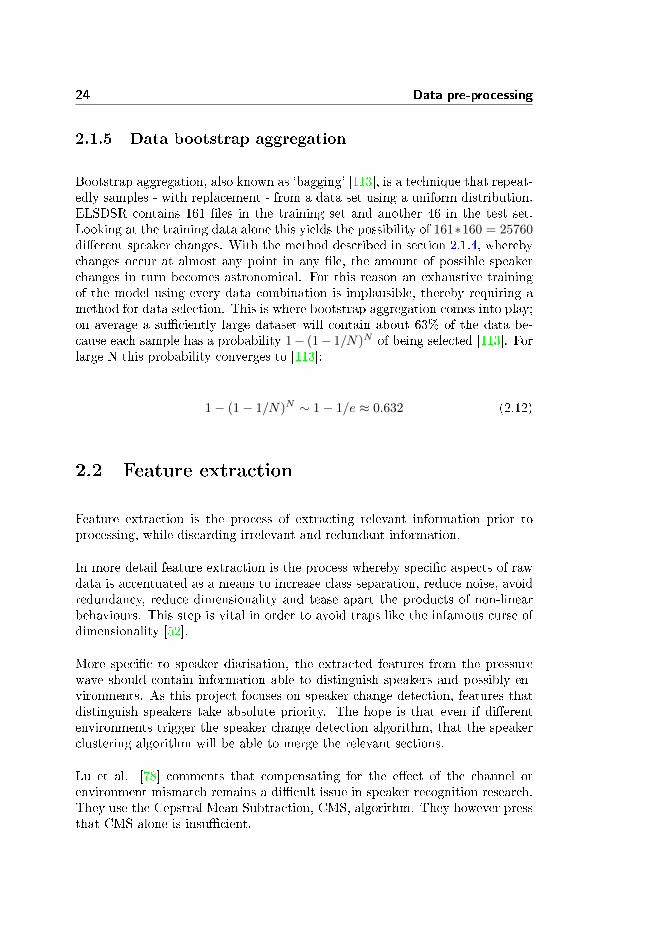
2.1.5 Data bootstrap aggregation
Bootstrap aggregation, also known as `bagging' [113], is a technique that repeat-edly samples - with replacement - from a data set using a uniform distribution.ELSDSR contains 161 �les in the training set and another 46 in the test set.Looking at the training data alone this yields the possibility of 161∗160 = 25760di�erent speaker changes. With the method described in section 2.1.4, wherebychanges occur at almost any point in any �le, the amount of possible speakerchanges in turn becomes astronomical. For this reason an exhaustive trainingof the model using every data combination is implausible, thereby requiring amethod for data selection. This is where bootstrap aggregation comes into play;on average a su�ciently large dataset will contain about 63% of the data be-cause each sample has a probability 1− (1− 1/N)N of being selected [113]. Forlarge N this probability converges to [113]:
1− (1− 1/N)N ∼ 1− 1/e ≈ 0.632 (2.12)
2.2 Feature extraction
Feature extraction is the process of extracting relevant information prior toprocessing, while discarding irrelevant and redundant information.
In more detail feature extraction is the process whereby speci�c aspects of rawdata is accentuated as a means to increase class separation, reduce noise, avoidredundancy, reduce dimensionality and tease apart the products of non-linearbehaviours. This step is vital in order to avoid traps like the infamous curse ofdimensionality [52].
More speci�c to speaker diarisation, the extracted features from the pressurewave should contain information able to distinguish speakers and possibly en-vironments. As this project focuses on speaker change detection, features thatdistinguish speakers take absolute priority. The hope is that even if di�erentenvironments trigger the speaker change detection algorithm, that the speakerclustering algorithm will be able to merge the relevant sections.
Lu et al. [78] comments that compensating for the e�ect of the channel orenvironment mismatch remains a di�cult issue in speaker recognition research.They use the Cepstral Mean Subtraction, CMS, algorithm. They however pressthat CMS alone is insu�cient.

2.2 Feature extraction 25
2.2.1 Feature type selection
Kinnunen et al. [62] compiled a list of appropriate properties that features forspeaker modelling and discrimination should have:
• Have large between-speaker variability and small within speaker variabil-ity.
• Be robust against noise and distortion.
• Occur frequently and naturally in speech.
• Be easy to measure from speech signal.
• Be di�cult to impersonate/mimic.
• Not be a�ected by the speaker's health or long-term variations in voice.
In addition to these, a �nal system must operate computationally e�cient andsince the number of required training samples for reliable density estimationgrows exponentially with the number of features, the number of features mustbe as low as possible in order to detect short speaker turns:
• Be computationally e�cient.
• Small feature vector size.
A range of feature types have been employed in the �eld of speaker diarisation[86]:
• Short Time Energy, STE, by Meignier et al. [84].
• Zero Crossing Rate, ZCR, by Lu et al. [79].
• Pitch by Lu et al. [77, 78].
• Spectrum magnitude by Boehm et al. [9].
• Line Spectrum Pairs, LSPs, by Lu et al. [78, 79].
• Perceptual Linear Prediction, PLP, cepstral coe�cients by Tranter et al.[114] and Chu et al. [19].

26 Data pre-processing
• Features based on phoneme duration, speech rate, silence detection, andprosody are also investigated in the literature Wang et al. [119].
Kinnunen et al. [62] categorise the features from the viewpoint of their physicalinterpretation:
1. Short-term spectral features.
2. Voice source features.
3. Spectro-temporal Features.
4. Prosodic features.
5. High-level features.
Then proceeds to recommend new researchers in the �eld of speaker changedetection to use only the �rst type. Namely short-term spectral features, on theargument that they incorporate all the properties above, are easy to computeand yield decent performance. Referencing the results by Reynolds et al. [101].
Mel-Frequency Cepstral Coe�cients, MFCCs, sometimes with their �rst andsecond derivatives are the most common features used (e.g. [23, 54, 79, 107]).
This project is built on the preliminary work for CastSearch by Jørgensen etal. [55] and Mølgaard et al. [87] which exclusively employs MFCCs. As theuse of MFCCs is quite common, literally recommended for new researchers andmediates direct comparison with previous work, this project will employ MFCCsas the sole features. Section 2.2.2 will go into detail on attributes and parametersof the MFCCs used in this thesis, section 2.2.3 looks at the largest limitation ofMFCCs and section 2.2.4 describes the underlying theory behind MFCCs.
2.2.2 MFCC attributes
For a description of the Mel-Frequency Cepstrum and the Mel-Frequency Cep-stral Coe�cients, see section 2.2.4 and 2.2.4.2.
Even though the use of MFCCs is very common, the range of MFCCs usedremains diverse. The use of 24-order MFCCs seems quite common [4, 17, 18, 115]while Kim et al. [60] applies 23-order MFCCs. Using derivatives is also common,13-order MFCCs along with their �rst-order derivatives are consistently applied
2.2 Feature extraction 27
by Kotti et al. [64, 66], while Wu et al. [122] employs 12-order MFCCs alongwith their �rst-order derivatives.
Understandably, in later work, various types of feature selection are being ap-plied to mitigate this issue. Wu et al. [122] investigates several MFCC ordersbefore the 12-order MFCCs along with their �rst derivatives are chosen. InKotti et al. [65], an e�ort is made to discover an MFCC subset that is moresuitable to detect a speaker change, with some performance gains, however theydo remark that this may reduce generalisability to other datasets. To furtherthis process this thesis applies several types of feature selection, see section 4.1and 4.3.1.
Also, there is no consensus with respect to �rst-order MFCC derivatives. While�rst-order MFCC derivatives are claimed to deteriorate e�ciency by Delacourtet al. [24], the use of �rst-order MFCC derivatives is found to improve perfor-mance by Wu et al. [122]. In this thesis this is found to depend on the appliedmethod's sensitivity to dimensionality issues, see section 4.1.1.2.
Since no consensus seems evident and since the 'direct comparison with previouswork' argument remains valid; this project will employ 12 MFCCs, with the useof �rst and second order derivatives and then perform forwards and backwardsfeature selection, see section 4.1 and section 4.3.1, respectively.
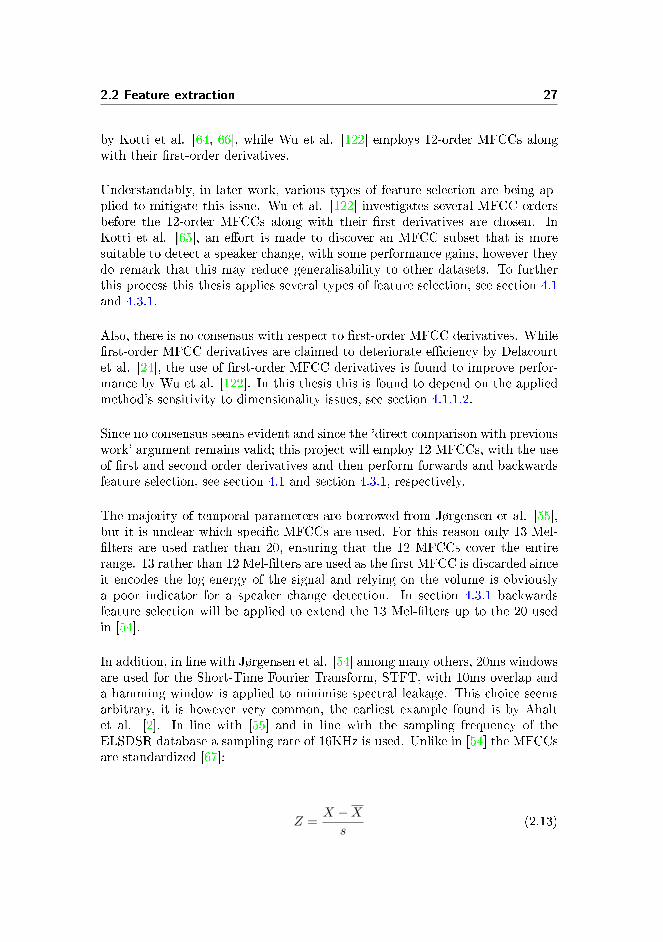
The majority of temporal parameters are borrowed from Jørgensen et al. [55],but it is unclear which speci�c MFCCs are used. For this reason only 13 Mel-�lters are used rather than 20, ensuring that the 12 MFCCs cover the entirerange. 13 rather than 12 Mel-�lters are used as the �rst MFCC is discarded sinceit encodes the log energy of the signal and relying on the volume is obviouslya poor indicator for a speaker change detection. In section 4.3.1 backwardsfeature selection will be applied to extend the 13 Mel-�lters up to the 20 usedin [54].
In addition, in line with Jørgensen et al. [54] among many others, 20ms windowsare used for the Short-Time Fourier Transform, STFT, with 10ms overlap anda hamming window is applied to minimise spectral leakage. This choice seemsarbitrary, it is however very common, the earliest example found is by Ahaltet al. [2]. In line with [55] and in line with the sampling frequency of theELSDSR database a sampling rate of 16KHz is used. Unlike in [54] the MFCCsare standardized [67]:
Z =X −Xs
(2.13)

28 Data pre-processing
Where Z is the standard score of a raw score X. X is the expected value of X,in this case a Gaussian is assumed reducing it to the sample mean, calculatedusing equation 3.9 and s is the standard deviation of X calculated using equation3.10.
This has been shown to improve performance in Viikki et al. [118].
2.2.3 MFCCs and noise
Despite the de facto standardization of their use as front-ends, MFCCs arewidely acknowledged not to cope well with noisy speech [16]. As written by Chenet al. [16], many techniques have been deployed to improve the performance inthe presence of noise, such as Wiener or Kalman �ltering [98, 116], spectralsubtraction [10, 33, 47, 48, 49], cepstral mean or bias removal [38, 56], modelcompensation [35, 88], Maximum Likelihood Linear Regression, MLLR, [121]and �nally the method applied by the inventors of the RuLSIF method, transfervector interpolation [92].
The general concept in all of these is to use prior knowledge of the noise to mask,cancel or remove noise during preprocessing or to adjust the relevant parametersto compensate for the noise. However it was realised that applying any of thesemethods is beyond the scope of this thesis. The necessary source code for addingvarious types of noise was designed, but testing the method chosen in section4.1 with it would require source code components that would simply take toolong to design and is therefore relegated to further work, see section 5.
The results found in this thesis is necessarily based on a relatively noise freeenvironment. In the context of news editing this should not pose a problem asspeaker transitions are rarely from one noisy environment to another. The SCDmethod found as optimal in this thesis will easily detect a change from a speakerin a noiseless environment to a speaker in a noisy environment, but might havedi�culties under changing noise conditions not coinciding with speaker transi-tions.
2.2.4 MFCC theory
As mentioned in section 2.2, this work is based solely on manipulation ofMFCCs.
The Mel-Frequency Cepstral Coe�cient, MFCC, features have been used in a

2.2 Feature extraction 29
wide range of areas. The Mel-Frequency Cepstrum, MFC, originates in speechrecognition [100], but has increasingly been used in other areas as well. Such asmusic genre classi�cation [3, 83], music/speech classi�cation [28, 89] and manyothers, for instance [32, 123].
The implementation used here is from the Voicebox toolbox by Brookes et al.[13]. This section will go into greater detail on the underlying theoretical aspects,by �rst examining the cepstrum, extraction of coe�cients using the DiscreetCosine Transform, DCT, and then moving onto a description of the Mel scaleand its applications.
2.2.4.1 The Cepstrum
This section is to a large degree based on the book, "Discrete-time processingof speech signals" by Deller et al. [25].
Speech in general can be modelled as a �ltering of the vocal excitation by thevocal tract, in other words a convolution in the time domain. The vocal excita-tion, produced by the vocal cords, controls the pitch and the volume of speech.Whereas the shape of the vocal tract controls the formants of speech whichde�ne literal semantics and nuances in the speech helpful for speaker discrimi-nation. Taking this into account is shown to improve performance in section 4.3.The speech signal, s(n), is therefore the vocal excitation, sometimes referred toas the excitation sequence [55], e(n), which is convolved with the slowly varyingimpulse response, θ(n), of the vocal tract:
s(n) = e(n) ∗ θ(n) (2.14)
An initial task in speech data preprocessing is therefore a deconvolution andseparation of these di�erent aspects of speech. This separation is useful fora number of reasons, mainly it enables the analysis of the separate aspectsindividually. This individual analysis is essential since the shape of the vocaltract control literal semantics and is thus useful in speech recognition, whereasthe vocal excitation is speaker speci�c and is therefore used mainly in speakerrecognition. Using all the data for SCD is shown to reduce performance insection 4.3.
This deconvolution is where the cepstrum comes into play, the cepstrum is a rep-resentation used in homomorphic signal processing, to convert signals combinedby convolution into sums of their cepstra, for linear separation. If the full com-

30 Data pre-processing
plex cepstrum is generated this process is termed `homomorphic deconvolution'[94, 99].
In the �eld of speech analysis the cepstrum is particularly useful as the low-frequency excitation and the the formant �ltering, which are convolved in thetime domain and multiples in the frequency domain, are additive and in di�er-ent regions in the quefrency domain. Quefrency being the independent variableof the cepstrum, analogues to frequency of the spectrum, in line with the ana-grammatic naming convention of the �eld.
The complex cepstrum, as described by [93], contains all phase informationand thereby enables signal reconstruction. However for application in speechanalysis, only the real cepstrum is standard and consequently the version im-plemented in Voicebox [13] and in this thesis employs this version. The realcepstrum, cs(n), is de�ned as [99]:
cs(n) = IDFT{log |DFT{s(n)}|} (2.15)
Where DFT and IDFT are the Discrete Fourier Transform and the InverseDiscrete Fourier Transform respectively and n is the time-like variable in thecepstral domain. Through the use of the Fourier transform the spectrum of thesignal becomes a multiplication of the components rather than a convolution:
S(k) = E(k)Θ(k) (2.16)
In practice a variation of the Short-Time Fourier transform, STFT, using over-lapping hamming windows is applied, see section 2.2.2. The logarithm productrule enables a linear separation of the components; thereby the multiplicationbecomes an addition, simultaneously the absolute value is used to discard allphase information:
log |S(k)| = log |E(k)Θ(k)| (2.17)
= log |E(k)|+ log |Θ(k)| (2.18)
= Ce(k) + Cθ(k) (2.19)
Finally to enter the quefrency-domain the IDFT is applied. Since IDFT isa linear operation it applies to each component according to the principle ofsuperposition, giving the real cepstrum of s(n), cs(n):

2.2 Feature extraction 31
cs(n) = IDFT{Ce(k) + Cθ(k)} (2.20)
= IDFT{Ce(k)}+ IDFT{Cθ(k)} (2.21)
= ce(n) + cθ(k) (2.22)
For a pictographical summary of the signal transformation process see �gure2.6.
2.2.4.2 Mel-frequency warping
The cepstrum described in section 2.2.4.1, is lacking a key feature often ap-plied, namely a frequency warping used to model the human auditory system.The general idea is that by applying this frequency warping the information ismore evenly distributed among the coe�cients. In [106] di�erent version areexamined and contrasted, including the one applied in the ISP toolbox [53]and therefore the one used here. The use of the Mel scale has been shown toincrease performance many times over and is standard practice in the �eld ofspeech analysis.
The calculation of the mel-cepstrum is similar to the calculation of the realcepstrum except that the frequency scale of the magnitude spectrum is warpedto the mel scale.
Originally proposed by Stevens et al. [110] the mel scale is a perceptual scaleof pitch. The scale is based on an empirical study of subjectively judged pitchratios by a group of test subjects.
It should be mentioned that among others Donald D. Greenwood, a student ofStevens, found the existence of hysteresis e�ects in the mel scale in 1956. Thisis mentioned in [109] and was submitted in a mailing list in 2009 [41]. The melscale does not take these hysteresis e�ects into consideration and is thereforeslightly biased, but has been shown to increase performance nonetheless.
The mel scale is usually approximated by a mapping with a single independentvariable, the corner frequency, i.e. the frequency to which the pitch ratio ismeasured against. This frequency have varied over the years, the currentlymost popular, and the version implemented in Voicebox [13], was proposed by[80] with a corner frequency of 700 Hz. The 700 Hz version superseded the 1000Hz version �rst proposed by [29], on the conclusion that it provides a closer

32 Data pre-processing
Figure 2.6: Shows how a speech signal is composed of a slowly varying envelopepart convolved with quickly varying excitation part. By moving tothe frequency domain, the convolution becomes a multiplication.Further taking the logarithm the multiplication becomes an ad-dition. Thereby neatly separating the components of the originalsignal in its real cepstrum. Figure borrowed from [25].

2.2 Feature extraction 33
approximation of the mel scale, especially at high and low frequencies [36]:
fmel = 2595 log10(1 +f
700) (2.23)
Where f is frequency.
Using this mel frequency mapping the MFCCs are calculated according to �gure2.7. In line with section 2.2.4.1, the only addition is the step for discretizingthe cepstrum, the discrete cosine transform. The MFCCs are computed fromthe Fast Fourier Transform, FFT, power coe�cients which are �ltered by atriangular band pass �lter bank. The �lter bank used in this thesis consists of12 triangular �lters later expanded to 20, see section 2.2.2. The MFCCs, Cn,are calculated as [99, 124]:
Cn =
√2
Kmel
Kmel∑k=1
(log10Sk) cos
(n(k − 1
2 )π
k
)(2.24)
Where Sk(k = 1, 2, . . . ,Kmel) is the outputs of the �lter bank and n = (1, 2, . . . , N)
are the samples in a 20ms audio unit. The√
2Kmel
normalisation factor is added
so that the inverse does not require an additional multiplicative factor, this isused to make the transform matrix orthogonal.
As mentioned in section 2.2.4.1, ideally only the vocal excitation part of thespeech signal is wanted and therefore only the highest coe�cients of the mel-cepstrum are extracted. As mentioned in section 2.2, this thesis initially uses allcoe�cients except the lowest from the 13 �lters, and subsequently �nd improvedresults by using only the 12 upper coe�cients from 20 �lters. In addition thisproject includes the �rst and second order derivatives of these coe�cients, asmentioned in section 2.2.
An interesting note is that some authors, including [23] have commented thatthe spectral basis functions of the cosine transform in the MFC are very similarto the principal components of the spectra, which were applied to speech rep-resentation and recognition much earlier by Pols et al. [97, 96]. Thereby givingcredit to the whole notion of MFCCs as a means to accurately represent spectralcontent e�ciently. Indeed it has even been found that MFCCs if produced froma very wide range of sounds, might be similar to an Independent ComponentAnalysis, ICA, of sound perceived by mammalian ears in general [43][71].

34 Data pre-processing
Figure 2.7: Process by which the MFCC features are calculated. This �gureis meant as an overview, not a summery, minor steps like win-dowing are overlooked for concision. Section 2.2.4 is dedicated toexplaining the process portrayed in this �gure.

2.3 Change-point detection 35
2.3 Change-point detection
The end goal is to hypothesize a set of speaker change-points, all methodshowever only produce a metric in which peaks correspond to possible change-points. This in essence boils the problem of change-point detection down toa need for a 1D-peak detection algorithm. In Jørgensen et al. [55] a suitablealgorithm is proposed, which includes a series of steps and a few free parameters.
A change-point is de�ned as a local, within Ti seconds, maxima above the thresh-old, Mcd. This threshold is the moving average over a region, 2 ∗ Tmax seconds,with a gain, αcd, applied to the threshold.
Mcd = αcd1
2 ∗ Tmax + 1
n+Tmax∑i=n−Tmax
metrici (2.25)
These free parameters Ti, Tmax and αcd need to be �xed or trained. This thesisde�nes a speaker turn as being above at least 1 sec. Therefore, in accordancewith [54], Ti is set to 2 seconds (other peaks within ±1 second are ignored).
In Jørgensen et al. [55], Tmax is used for multiple purposes, in addition tode�ning a length for the moving average it de�nes the maximum use of data inthe False Alarm Compensation algorithm, FAC. A discussion of why and howTmax is determined will be delineated in section 2.4, after the FAC method hasbeen explained.
The threshold gain parameter, αcd, is trained empirically through a search, inthe free parameter space, for a maximal F-measure, see section 3.3.
2.4 False Alarm Compensation
The common approach to speaker change detection is that of a comparisonbetween subsequent segments of a �xed length [54][111][105]. This approachhowever is saddled with an inherent problem, namely the ability to detect shortspeaker turns, requiring short analysis windows, versus the ability to avoid falsepositives, requiring long analysis windows, see section 1.1.3. The literatureproposes several solutions to this dilemma.
• Algorithms that successively build larger segments rather than comparing

36 Data pre-processing
equal sized segments [42].
• Methods for running several analysis window lengths in parallel and thencombining the results [7].
• Iterative methods, where the algorithm is run recursively with successivelylonger analysis windows on the successively smaller amount of possiblechange-points in order to reject false alarms. This class of methods hasbeen termed False Alarm Compensation, FAC, and is employed by [54].Here the false alarm compensation step was run only once.
This project employs a variant of the FAC method employed in Jørgensen etal. [54], the di�erence being an investigation into the bene�t of a multistepprocedure, here termed Recursive FAC, RFAC, see section 2.4.1 and 5.2.
This approach has a number of free parameters; A bu�er variable equal to Ti,see section 2.3 used as a bu�er zone around a hypothesized change-point, athreshold gain parameter, αFAC , and �nally, Tmax, the maximum data usedfrom available data on each side of a hypothesized change-point.
αFAC is a gain applied to the moving average threshold calculated on the met-ric, MFAC , similar to the variable, αcd, see section 2.3. αFAC times this movingaverage threshold is the function below which a hypothesized change-point isrejected. Only two thresholds exist, the change-detection one which is the mov-ing average of the metric with the gain αcd, and the same moving average withthe gain αFAC .
MFAC = αFAC1
2 ∗ Tmax + 1
n+Tmax∑i=n−Tmax
metrici (2.26)
The threshold gain parameter, αFAC , is trained empirically through a search,in the free parameter space, for a maximal F-measure, see section 3.3.
In Jørgensen et al. [55] it is argued that in order to maintain correlation betweenthe FAC threshold and the change-point threshold, Tmax, the maximum analysiswindow and length of the moving average must be identical across algorithms.
Tmax has the additional purpose of maintaining speaker turn purity. I.e. if aspeaker-change point is missed during the �rst iteration, the resulting speakerturn data would contain multiple speakers. Tmax counteracts this issue by usingthe data closest to the hypothesized change-point in question, thus using as much

2.4 False Alarm Compensation 37
data from the true speaker as possible and completely purifying the data if thetrue speaker turn is longer than Tmax.
2.4.1 Hybrid method
This section will slightly modify the basic FAC method mentioned in section 2.4,by proposing a robust novel approach where metrics are combined to compensatefor dissimilar weaknesses. A novel approach is proposed as a literature searchfailed to yield any solutions to the problems described in this section.
In section 4.1.3.1, it is shown that combining di�erent metrics could potentiallyincrease performance, the reason being that they might be able to complementeach other on several key points. As mentioned in section 2.4, the idea of afalse alarm compensation paradigm is to incrementally increase the amount ofdata available to the metric to progressively re�ne its estimate at a potentialchange-point, using the earlier iterations to determine how much data is actuallyavailable. During these iterations potential change-points that are found to befalse alarms are deleted freeing up data for neighbouring potential change-points.
The metrics, see section 3.2, vary in computational complexity and performance,with the computationally heavy metrics generally outperforming the light met-rics, see section 4.1.3. Using a light metric to quickly detect a large amount ofpotential change-points and then subsequently applying a heavy metric on thesmall data set to �lter out the false alarms seems logical.
This combined metric approach however has a serious issue at its core. In thestandard FAC paradigm the FAC threshold is merely a scaled version of thethreshold applied in the change-detection step, see section 2.4. As the samemetric is usually applied to both change-detection and FAC the only di�erenceis in the amount of data the metric is working with. I.e. in the standard FACparadigm it is assumed that the FAC metric assumes roughly the same rangeof values as the change-detection metric irrespective of the amount of data usedand that peaks will merely be scaled versions depending on the data amount.
When combining metrics both of these assumptions fail and must be handled.The novel approach proposed here involves discarding the notion of using themoving-average of the change-detection step in the FAC step altogether.
Ideally the FAC metric is only evaluated at potential change-points, this howeverposes a problem as a reference is required in order to determine a threshold towhich the FAC metric is compared. As one of the strengths of the combinedmetric approach is that they treat the data di�erently, i.e. accentuating di�erent

38 Data pre-processing
aspects, using a threshold based on a scaled version of the change-detectionmetric is invalid.
What is proposed instead is a heuristic for estimating a noise �oor of the FACmetric through information gathered from the change-detection step. The basicassumption is that if the change-detection metric has a low threshold, therebyproposing a large amount of potential change-points, then a position far from apotential change-points is very unlikely to actually be a change-point.
The Combined Metric FAC, CMFAC, is therefore given the list of potentialchange-points along with a list of not-change-points. It is then saddled withthe job of identifying which of the potential change-points are di�erent enoughfrom the not-change-points. These not-change-points are chosen as close to thecenter as possible between the proposed change-points.
This novel CMFAC method applies its particular metric, RuLSIF is used insection 5.2, to each of the not-change-points using as much data as possible upto Tmax, in exactly the same fashion as the standard FAC method, see section2.4. Thereby acquiring a list of values that probably correspond to the noise�oor of the CMFAC metric. This list might however still contain change-pointsor other rare events, this is handled by taking the median of this list, therebyacquiring a single value very likely to be representative of the noise �oor.
This single value is then used as a constant threshold to which the gain, αFAC ,is trained, see section 3.3. The hope is that the disadvantage of trading themoving average threshold of standard FAC for the constant median threshold ofthe CMFAC approach will be out weighted by the bene�t of a more expensiveand more thorough metric. A metric that does not have to correspond to themetric used in the change-detection step.
This median approach is chosen as that will enable the algorithm to apply even inthe case of news editing, where only a few speaker changes occur. The CMFACmethod is applied in section 5.2, with KL and RuLSIF used as change-detectionmetric and CMFAC metric respectively. There the performance is compared tostandard FAC using KL with KL and RuLSIF with RuLSIF.

Chapter 3
Methodology
This chapter will delineate the theoretical ground work. To begin with, a shortintroduction to the concept of metrics and how they relate to the actual sound,is bridged using a spectrogram and a graphical representation of the MFCCs.Once this is in place, the independent approaches to SCD are described in detail,these include; Vector Quantization, Gaussian based approaches and RelativeDensity Ratio Estimation.
This chapter will then describe the parameter optimisation technique used totrain the change detection and the FAC thresholds. These methods are appliedin section 4.1.2. Finally this chapter will conclude with some miscellaneous basicrequired theory.
3.1 Metric introduction
This section will try to bridge the gap from sound pressure up one abstractionlevel to the SCD F-measure score using the various methods.
The upper graph seen in �gure 3.1 shows a spectrogram of some speech data,i.e. with frequency on the y-axis, time on the x-axis and magnitude encoded in

40 Methodology
the color scale going from blue, low, to red, high. The speech is recognisablyproducing patterns, but obviously distinguishing between speakers is di�cult atbest.
Using the feature extration methods described in section 2.2; The MFCCs areshown in the middle graph which to a large degree resembles noise, but mostassuredly contains SCD cues. Slightly confusingly the frequency scale in themiddle graph is an inverted version of the upper graph, this is a remnant of analignment process which was more straightforward this way and given that theMFCCs are standardized the relevance is negligible.
The bottom graph displays the metrics of the various methods applied to theMFCCs and here the speaker changes are obviously very detectable. The hori-zontal dotted green lines represent actual changes from one speaker to another,the red ones denote changes between �les containing the same speaker, theseare obviously invalid and should not get detected. The metrics are designed topeak at speaker changes and are independent of the green and violet circles.
These green and violet circles represent the change-detection and FAC algo-rithms respectively applied to the metrics, with a green simply signifying thatthe algorithm thinks it encountered a speaker change, not denoting the success.The violet circles represent potential speaker change-points - formerly green cir-cles - that the FAC algorithm has �agged as false alarms. Note that a potentialchange-point must be within 1 second of the actual change to count towards theF-measure score seen in the legend. The F-measure being the harmonic meanbetween hits-to-tries ratio and hits-to-possible-hits ratio.
3.2 Speaker dissimilarity metrics
To determine the dissimilarity of two subsequent analysis windows a suitabledissimilarity metric must be chosen. In the literature many such measures havebeen proposed, in this project some of the most common approaches are singledout and compared, this section will describe the theory behind these and thelimitations of them. The metrics will then be trained, see section 4.1.2, andcompared using test data, see section 4.1.3, to determine their performance inthe context segment comparison and false alarm compensation. In must benoted that alternatives to the metric based approach, when comparing analysiswindows, are used in the literature, but will not be tested in this thesis. As anexample Henkel et al. [46] compares distributions in the framework of hypothesistesting.

3.2 Speaker dissimilarity metrics 41
Figure 3.1: The upper graph shows a spectrogram of the data, i.e. with fre-quency on the y-axis, time on the x-axis and magnitude encodedin the color scale going from blue, low, to red, high. The standard-ized MFCCs are shown in the middle graph. Slightly confusinglythe 'frequency scale' in the middle graph is an inverted version ofthe upper graph. The bottom graph displays the various metricsapplied to the MFCCs. The horizontal dotted green lines rep-resent actual changes from one speaker to another, the red onesdenote changes between �les containing the same speaker, theseare obviously invalid and should not get detected. The metricsare designed to peak at speaker changes and are independent ofthe green and violet circles. These green and violet circles repre-sent the change-detection and FAC algorithms respectively, with agreen simply signifying that the algorithm thinks it encountered aspeaker change, not denoting the success. The violet circles repre-sent potential speaker change-points that the FAC algorithm has�agged as false alarms. As seen the FAC algorithm does fairlywell, but sometimes marks correct change-points as false alarms,see upper right on bottom �gure. Note that a potential change-point must lie within 1 second of the actual change to count to-wards the F-measure score seen in the legend. The F-measurebeing the harmonic mean between the hits-to-tries ratio and hits-to-possible-hits ratio.

42 Methodology
3.2.1 Vector Quantization
Vector quantization, VQ, [39, 40] incorporates a variety of approaches to 'dis-cover' the underlying structure of a dataset through iteratively improved guesses.More technically VQ is a central topic in signal processing, a sub-�eld of com-petitive learning and deals with the problem of representing a dataset by meansof a smaller, �nite size, K, codebook of representative data points or 'centroids'[50]. The size of K must be chosen to match the application and how the cen-troids are initially chosen as well as how they are updated depends on the choiceof algorithm. An example of a simple VQ algorithm could be:
1. Pick a sample point at random.
2. Move the nearest centroid towards this sample point.
3. Go to step 1.
An input belongs to cluster i if i is the index of the closest centroid, here distanceis measured using the Euclidean distance. This has the e�ect of dividing up thespace into a Centroidal Voronoi tesselation, CVT, a high dimensional beehive-esque structure where the cells size is inversely proportional to the data densityand the shape is determined by the proximity to other cells [26].
Many di�erent algorithms for various purposes have been designed, within the�eld of speaker diarisation VQ has found its uses in many di�erent aspects, suchas word recognition [14], speaker recognition [108], and of cause speaker changedetection [54].
3.2.1.1 Choice of algorithm
This section will describe the VQ algorithm choice, for a description of the choicesee section 3.2.1.2.
Within the �eld of VQ there are two distinct groups of algorithms, the on-linealgorithms and the batch algorithms. Batch algorithms recomputed all valuesat each iteration, whereas on-line algorithms compute only a single value eachiteration. An example of this distinction is the standard K-means [8] vs. the socalled Winner-Takes-All, WTA, version of K-means [45].
On-line does not necessarily refer to new data coming in, as VQ is sensitiveto sequential data that is non-i.i.d. - independent and identically distributed -these centroids chosen for updates are either randomly or carefully selected [45].

3.2 Speaker dissimilarity metrics 43
On-line methods that update sequentially on incoming data are not directlyapplicable in the context of speech as the signal varies far too quickly to beof practical use, beyond this the common approach, when analysing temporale�ects in the signal, is to use derivatives of the input along with the input, thisis discussed in section 2.2.
Ahalt et al. [2] compares several algorithms in the context of speech data,but �nds no signi�cant di�erence in performance, signifying that the particu-lar choice of training algorithm is to some degree irrelevant performance wise.The algorithms included the Self Organizing Maps [63], SOM, the Frequency-Sensitive Competitive Learning, FSCL, algorithm neural network [50, 108] andthe Linde�Buzo�Gray algorithm, LBG, [73]. The LBG algorithm is an extensionof Lloyd's algorithm [76] and similar to the more well-known K-means algorithm[8]. The result is similar in another study, this time by Kinnunen et al. [61],where �ve di�erent clustering algorithms are compared for use in a speaker iden-ti�cation setup using vector quantization. The comparison shows only marginaldi�erence in the results obtained with the �ve algorithms.
Beyond performance this still leaves attributes like e�ciency, robustness andconvergence. In lieu of other work that compares di�erent algorithms, a ro-bust common choice must be made. The previous work this project builds onJørgensen et al. [55] used a version of the K-means algorithm and proposedsome optimisations, see section 3.2.1.4, along with �nding overall decent resultsusing it. For this reason the K-means algorithm will be employed for use inVQ. The convergence properties, the limitations and the general principals ofthe K-means algorithm will be discussed in the following subsections.
3.2.1.2 K-means
Given a dataset {x1, . . . , xn} consisting of N observations of arbitrary dimen-sionality. The goal of K-means is to group the data into K pure clusters with theminimum within-cluster sum of squares, WCSS, distance. As such the objectivefunction for K-means is given as [8]:
WCSS =
N∑n=1
K∑k=1
rnk||xn − µk||2 (3.1)
Where µk are the cluster centroids and rnk is a vector signifying to which clusterxn belongs:

44 Methodology
rnk =
{1 if k = argminj ||xn − µk||2
0 otherwise.
This objective function is also referred to as a distortion measure by bishop [8]and is also used as the metric to quantify the change in the signal, see section3.2.1.3.
The objective of the K-means algorithm is to solve the NP-hard problem [6] of�nding the optimal combination of µk and rnk for minimising WCSS heuristi-cally.
This heuristic is a 2-step procedure similar to the more general EM-algorithm [8]used in the also very established Gaussian Mixture Model, GMM, [8] approachwhich has also found its uses in SCD [68, 81]. The GMM approach was originallyincluded in this thesis, but was cut both for e�ciency reasons and due to thedi�culty in de�ning a suitable dissimilarity metric, which lead to the �eld ofthe Adapted Gaussian Mixture Models, AGGM, [81] or out of this paradigmaltogether into the Hidden Markov Model, HMM, [68].
The basis of this heuristic is the fact that a closed form solution of the objectivefunction is easily found looking at a speci�c cluster k, Ck. The objective function3.1 is quadratic in µk and therefore convex, meaning that a local minimum isthe global minimum. The minimum is found by minimising the derivative ofWCSS with respect to µk:
dWCSSdµk
=
N∑n=1
K∑k=1
2rnk(xn − µk) = 0 (3.2)
Where µk is just the arithmetic mean of xn found by solving for µk:
µk =
∑Nn=1 rnkxn∑Nn=1 rnk
(3.3)
Since the denominator is the total number of points in cluster k, Sk, and thenumerator is the sum of all points in cluster k, Ck:
µk =
∑xn∈Ck xn
Sk(3.4)

3.2 Speaker dissimilarity metrics 45
This is also the reason why the method is called K-means.
Using this closed form solution a local minima to the NP-hard problem [6] isfound using this algorithm [8]:
• Initialisation step: Initially Initialise centroids using Forgy's method[34], which simply uses k data points drawn at random. On subsequentanalysis windows use previous centroids, see section 3.2.1.4.
• Assignment step: Assign each data point to the cluster whose centroidis closest to it. Where each data point xn belongs to only one cluster,which is not a problem here as the distance measure used is Euclidean.
If any cluster is empty, reinitialise it using the singleton method, i.e. moveit to the data point furthest from all centroids.
• Update step: Calculate the new position for the centroids of each clusterusing equation 3.4.
If the stopping criterion is not met, return to the assignment step.
• Stopping criteria: The algorithm has converged when the no centroidswere moved. This stopping criteria is shown in [11] to be stable, but as afail-safe the algorithm will stop if a large maximum number of iterationshave passed.
The MATLAB function kmeans from the statistics toolbox is used to implementK-means [82].
3.2.1.2.1 Limitations of K-means
K-means as a method for clustering has some stringent limitations that must tobe addressed.
In particular K-means in the context of clustering has problems [8] when clustershave:
• Di�ering sizes
• Di�ering densities
• Non-globular shapes
• Outliers

46 Methodology
Most of these concerns however are not as crucial here as K-means is used toapproximate the underlying probability density function, PDF, not to identifymeaningful clusters in the data.
As seen in �gure 2.2 the data in the MFCC space is roughly globular, butdoes contain some outliers. What these outliers signify and by extension whatindividual clusters found by K-means signify is not investigated in this thesis.
These limitations do however limit K-means' ability to approximate nuances inthe PDF and will therefore skew the results slightly as a di�erence between sub-sequent analysis windows might not be representative of the underlying PDF,but in how K-means approximates it. How this a�ects the results is not inves-tigated in this thesis, however this issue is inverse proportional to the size of K,see section 4.1.1.3.2 for selection of codebook size.
Beyond this K-means have di�culties when unfortunate initialisation or iter-ations results in empty clusters. This thesis applies the singleton approachwherein empty clusters are assigned to the data point furthest from any cen-troid. This singleton approach obviously makes the K-means method even moreoutlier sensitive. The larger the codebook is the more likely it is that an outlierwill be assigned as its own cluster, but the less likely it is that it will signi�-cantly impact that approximation. This issue however is mitigated due to howdi�erences between codebooks are calculated, see section 3.2.1.3, since a clusteris merely compared to its closest neighbour in the previous codebook, not itsprevious position.
3.2.1.2.2 Codebook size
The choice of codebook size, K, and feature selection in the context of K-meansis investigated in section 4.1.1.3.
3.2.1.3 Choice of metric
Given that the analysis windows are clustered using the K-means algorithmdescribed in section 3.2.1.2, a crucial step remains, which is a choice of metric forcomparing windows. Since the K-means algorithm is designed to minimise theWCSS, the obvious choice is to use the previous analysis window as training dataand the subsequent analysis window as test data, thereby directly measuring theWCSS using equation 3.1.
This approach has been termed Vector Quantization Distortion, VQD, by Nak-
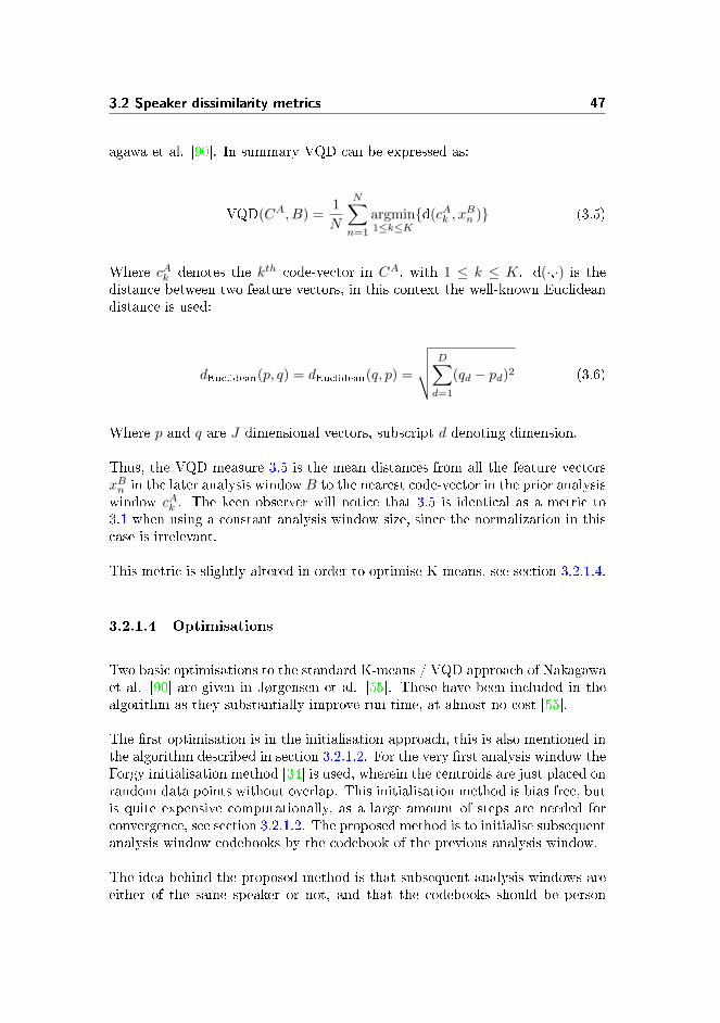
3.2 Speaker dissimilarity metrics 47
agawa et al. [90]. In summary VQD can be expressed as:
VQD(CA, B) =1
N
N∑n=1
argmin1≤k≤K
{d(cAk , xBn )} (3.5)
Where cAk denotes the kth code-vector in CA, with 1 ≤ k ≤ K. d(·,·) is thedistance between two feature vectors, in this context the well-known Euclideandistance is used:
dEuclidean(p, q) = dEuclidean(q, p) =
√√√√ D∑d=1
(qd − pd)2 (3.6)
Where p and q are J dimensional vectors, subscript d denoting dimension.
Thus, the VQD measure 3.5 is the mean distances from all the feature vectorsxBn in the later analysis window B to the nearest code-vector in the prior analysiswindow cAk . The keen observer will notice that 3.5 is identical as a metric to3.1 when using a constant analysis window size, since the normalization in thiscase is irrelevant.
This metric is slightly altered in order to optimise K-means, see section 3.2.1.4.
3.2.1.4 Optimisations
Two basic optimisations to the standard K-means / VQD approach of Nakagawaet al. [90] are given in Jørgensen et al. [55]. These have been included in thealgorithm as they substantially improve run time, at almost no cost [55].
The �rst optimisation is in the initialisation approach, this is also mentioned inthe algorithm described in section 3.2.1.2. For the very �rst analysis window theForgy initialisation method [34] is used, wherein the centroids are just placed onrandom data points without overlap. This initialisation method is bias free, butis quite expensive computationally, as a large amount of steps are needed forconvergence, see section 3.2.1.2. The proposed method is to initialise subsequentanalysis window codebooks by the codebook of the previous analysis window.
The idea behind the proposed method is that subsequent analysis windows areeither of the same speaker or not, and that the codebooks should be person

48 Methodology
speci�c. This means that if the previous codebook was not a good approximationof the next analysis window, then a large change in the codebook should occur,signifying a speaker change. This optimisation improves the run-time by a factorof about 2.5 using a codebook size of K = 56.
The second optimisation applies the assumption that the codebook of an analysiswindow is a fair approximation of said analysis window. Thereby replacing alldata points, xBn , in equation 3.5, with the codebook for analysis window B, CBk :
VQDOptimised(CA, CB) =1
N
N∑n=1
argmin1≤k≤K
{d(cAk , cBk )} (3.7)
This assumption is the basic assumption of VQ in general, see section 3.2.1 andis therefore a logical necessity. This optimisation improves the run-time by afactor of about 7, using K = 56, see section 4.1.1.3.2 for choice of codebook size.
In total these optimisations improve the run-time of the K-means algorithm by afactor of about 15, enabling its use, for a deeper analysis into the computationale�ciency of the various approaches compared to real time, see section 4.1.3.2.
3.2.2 Gaussian based approaches
This section will describe the second group of approaches tested in this projectin the context of SCD, which is the single multivariate Gaussian approach, alongwith its individual sub constituents. This approach is common in the contextof SCD, and has been shown to perform decently [54, 85].
This approach is basically modelling each analysis window as being drawn fromits individual multivariate Gaussian and then comparing analysis windows bythe distortion of the estimated underlying PDF. These distortion measures in-clude the Kullback-Leibler distance, KL, and its constituents, the DivergenceShape Distance, DSD, and the Euclidean distance between the sample means.
The distance between sample means is implemented using VQ and a K-meansalgorithm with a codebook size of K = 1, in which case it degenerates intothe Euclidean distance between sample means, see section 4.1.1.2. The sectionsbelow will describe the KL and DSD dissimilarity measures, 3.2.2.3 and 3.2.2.4respectively.

3.2 Speaker dissimilarity metrics 49
3.2.2.1 Estimation of population parameters
A multivariate Gaussian distribution has two population parameters, the pop-ulation mean, µ, and the population covariance matrix, Σ, and is given by [8]:
N (x|µ,Σ) =1
(2π)D2
1√|Σ|
exp
(−1
2(x− µ)TΣ−1(x− µ)
)(3.8)
Where D is the number of dimensions, x is a D-dimensional vector in the MFCCspace, xT and x−1 signi�es the transpose and inverse of x respectively and �nallythe population parameters µ and Σ which must be estimated empirically.
The population mean is estimated using the sample mean [8], which is basicallythe arithmetic mean of every dimension individually:
x =1
N
N∑i=1
xi (3.9)
Where N is the sample size.
The calculation of the sample covariance matrix is slightly more complicated,as it has the disadvantage of being very prone to outliers [51, 117]. Section2.1.3.1 analysis how prone the MFCC data is to outlier behaviour, as seen,outliers are rare and the data follows a multivariate normal distribution to agood approximation. For this reason an unbiased estimator of the covariancematrix is used and is given by [8]:
qjk =1
N − 1
N∑i=1
(xij − xj)(xik − xk) (3.10)
Where qjk are the entries of the sample covariance matrix, Q, Which is just theaverage covariance of every pair of dimensions, where N − 1 is used rather thanN , since a D.o.F was spent calculating the sample mean. This is implementedusing the MATLAB function cov.
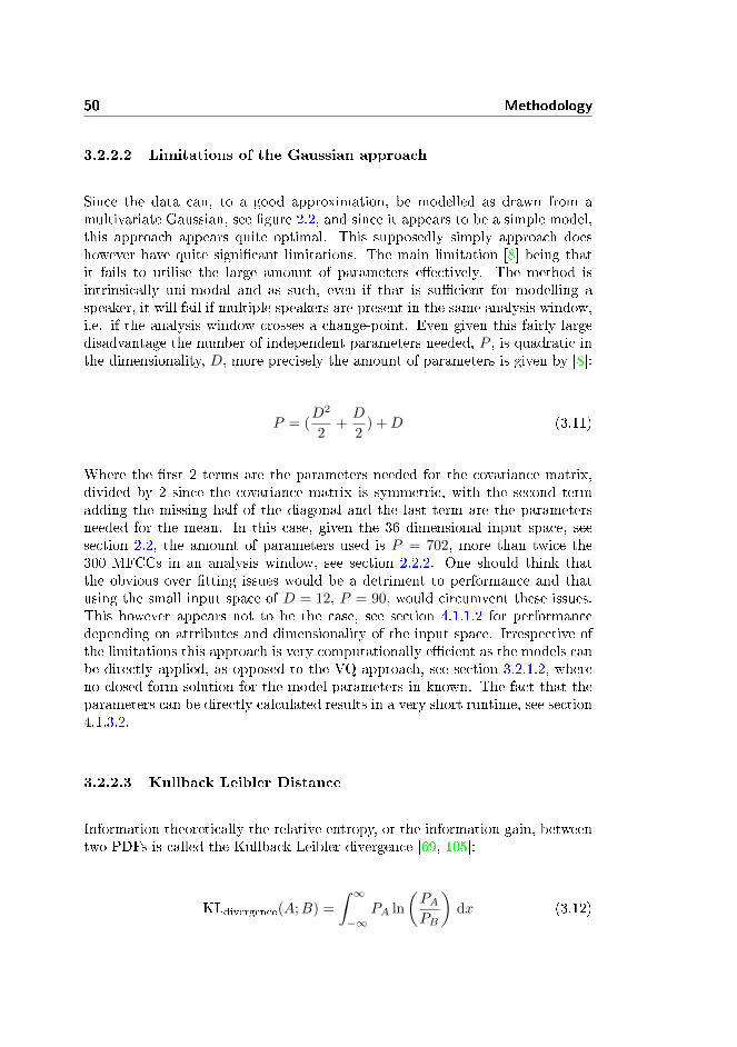
50 Methodology
3.2.2.2 Limitations of the Gaussian approach
Since the data can, to a good approximation, be modelled as drawn from amultivariate Gaussian, see �gure 2.2, and since it appears to be a simple model,this approach appears quite optimal. This supposedly simply approach doeshowever have quite signi�cant limitations. The main limitation [8] being thatit fails to utilise the large amount of parameters e�ectively. The method isintrinsically uni-modal and as such, even if that is su�cient for modelling aspeaker, it will fail if multiple speakers are present in the same analysis window,i.e. if the analysis window crosses a change-point. Even given this fairly largedisadvantage the number of independent parameters needed, P , is quadratic inthe dimensionality, D, more precisely the amount of parameters is given by [8]:
P = (D2
2+D
2) +D (3.11)
Where the �rst 2 terms are the parameters needed for the covariance matrix,divided by 2 since the covariance matrix is symmetric, with the second termadding the missing half of the diagonal and the last term are the parametersneeded for the mean. In this case, given the 36 dimensional input space, seesection 2.2, the amount of parameters used is P = 702, more than twice the300 MFCCs in an analysis window, see section 2.2.2. One should think thatthe obvious over �tting issues would be a detriment to performance and thatusing the small input space of D = 12, P = 90, would circumvent these issues.This however appears not to be the case, see section 4.1.1.2 for performancedepending on attributes and dimensionality of the input space. Irrespective ofthe limitations this approach is very computationally e�cient as the models canbe directly applied, as opposed to the VQ approach, see section 3.2.1.2, whereno closed-form solution for the model parameters in known. The fact that theparameters can be directly calculated results in a very short runtime, see section4.1.3.2.
3.2.2.3 Kullback Leibler Distance
Information theoretically the relative entropy, or the information gain, betweentwo PDFs is called the Kullback-Leibler divergence [69, 105]:
KLdivergence(A;B) =
∫ ∞−∞
PA ln
(PAPB
)dx (3.12)

3.2 Speaker dissimilarity metrics 51
This measure is not directly applicable as a metric, as it is a divergence and isobviously not symmetric. This is handled by introducing the notion of RelativeCross Entropy [105], or in common parlance the Kullback Leibler distance, oftenabbreviated KL2, here for practical reasons referred to simply as KL. The Kull-back Leibler distance merely solves the issue by looking from both directions atonce:
KLdistance(A;B) = KLdivergence(A;B) + KLdivergence(B;A) (3.13)
=
∫ ∞−∞
(PA − PB) ln
(PAPB
)dx (3.14)
A full derivation of the Kullback Leibler distance can be found in the originalwork by Kullback and Leibler [69].
Inserting equation 3.8 into 3.13 and moving into the discrete domain, yields [55]:
KLdistance(A;B) =1
2Tr[(ΣA − ΣB)(Σ−1A − Σ−1B )
]+
1
2Tr[(Σ−1A − Σ−1B )(µA − µB)(µA − µB)T
](3.15)
This is the implemented version of the Kullback-Leibler distance, see appendixA.3.2. The Kullback-Leibler distance has been applied broadly, with decentperformance, in the �eld of speaker diarisation [54, 85, 105].
3.2.2.4 Divergence Shape Distance
In Lu et al. [78] it was found that environment to a large degree is encodedin the position of the Gaussian in space, or its mean. To circumvent this theKullback-Leibler distance 3.15 was applied without the second term involvingthe means, a measure called the Divergence Shape Distance, DSD:
DSD(A;B) =1
2Tr[(ΣA − ΣB)(Σ−1A − Σ−1B )
](3.16)
As such the DSD is used as a metric for determining the divergence of thecovariance matrix. All data in this project, see section 2.2.3, is as environment-free as possible, given that it is not recorded in an anechoic chamber. To avoid

52 Methodology
any e�ects the environment could have on the performance, code was developedfor applying various noise types, but due to lack of resources this has beenrelegated to further work in section 5. The DSD measure is however included todetermine whether excluding the means improves the performance even in anenvironment free setting. This appears to not be the case, see section 4.1.1.2.
3.2.3 Relative Density Ratio Estimation
The �eld of change-detection in general is vibrant with new methods and ap-proaches. This section will describe how and why a novel approach developmentby Liu et al. [75] is applied. Let it be noted that for unreferenced statementsin this section [75] is implied.
The other applied approaches, see section 3.2.1 and 3.2.2, su�er from a core de-�ciency that this new approach circumvents. They estimate individual modelsfor the preceding and the succeeding analysis windows, then subsequently esti-mate the di�erence between these, discarding the individual models, see �gure1.2. This section will describe a novel approach in the �eld of change-detectionthat directly estimates the relative density-ratio. The applied method is calledRelative unconstrained Least-Squares Importance Fitting, RuLSIF, and is anextension of the more comprehensible Kullback-Leibler Importance EstimationProcedure [112], KLIEP, by Sugiyama et al.
RuLSIF was introduced to overcome certain de�ciencies of KLIEP. These de-�ciencies are mainly extreme sensitivity to outliers, see section 3.2.3.1.1, andthe lack of a closed-form solution [112]. Along with the avoidance of thesede�ciencies RuLSIF provides a set of advantages, these include; an improvednon-parametric convergence rate [57, 125], numerical stability [58] and robust-ness [111].
This section will �rst outline KLIEP and its relation to the KL method describedin section 3.2.2.3, as well as proceed to extent KLIEP to the full RuLSIF method.
3.2.3.1 From KLIEP to RuLSIF
The KLIEP method is related to the KL method described in section 3.2.2.3, inthat it is based on the KL-divergence. KLIEP however takes a non-parametricapproach and directly approximates a measure similar to the KL distance.
The essence of the density-ratio estimation is the notion of a function, g(x|θ),

3.2 Speaker dissimilarity metrics 53
called the density-ratio that when multiplied by the PDF of the succeedinganalysis window, PB yields the PDF of the preceding analysis window, PA:
PA = g(x|θ)PB (3.17)
⇔
g(x|θ) =PAPB
(3.18)
In other words estimating the density-ratio, g(x|θ), can be expressed as anoptimisation problem, whereby g(x|θ) is estimated through a minimisation ofthe KL-divergence 3.12:
KLdivergence(A;B) =
∫PA log10
(PA
PBg(x|θ)
)dx (3.19)
Where the PDFs, PA and PB are functions of x. To elaborate; in practice g(x|θ)is approximated as seen below, 3.22, if approximated ideally the KLdivergence(A;B)is naturally:
KLdivergence(A;B) =
∫PA log10 (1) dx = 0 (3.20)
Indicating no information gain from PA to g(x|θ)PB .
The reader will have noticed that the logarithm base has changed from 3.12to 3.19. To dispel confusion it must be noted that the KL divergence holdsirrespective of log base [69]. Logarithms in these formulae are taken to base 2 ifinformation is measured in units of bits and to base e if information is measuredin nats. Too simplify the implementation the version used here uses base 10 aschosen by Liu et al. in [75] on which the work here is based.
The trick then is that by the quotient logarithm rule [1] the unknown PDFs PAand PB can be ignored:
KLdivergence(A;B) =
∫PA log10
(PAPB
)dx−
∫PA log10(g(x|θ)) dx (3.21)

54 Methodology
As they are irrelevant to g(x|θ) and as the second term for obvious reasonscannot exceed the �rst term, since that would result in the approximation re-sembling the function more than the function itself. Since the �rst term mustbe positive and has no parameters, the only way to minimise 3.21 is to minimisethe second term.
In KLIEP as well as RuLSIF the density-ratio, g(x|θ), is modelled using a kernelmodel:
g(xA|θ) =
N∑i=1
θiK(xA, xBi ) (3.22)
Where N is the number of samples in an analysis window and where θ =(θ1, . . . , θN )T , are the parameters to be learned via the mentioned optimisa-tion problem 3.21. For the kernel basis function the Gaussian kernel is applied:
K(xA, xB) = exp
(−||x
A − xB ||2
2σ2
)(3.23)
Where σ is the kernel width trained for each density-ratio individually, seesection 3.2.3.2 for more details.
Inserting 3.23 into 3.21 yields a convex optimisation problem which in the case ofKLIEP lacks a closed form solution and therefore requires an iterative approach[75]. This optimisation yields the estimate of the density-ratio, g(x|θ).
Finally given this estimate of the density ratio, the estimate of the KL-divergencecan be approximated as the arithmetic mean of the log density ratio [59]:
KL =1
n
n∑i=1
log10 g(x|θ) (3.24)
Where n is the number of samples in an analysis window.
3.2.3.1.1 Outlier sensitivity of KLIEP
The main reason KLIEP is not applied is its extreme sensitivity to outlierswhich for lack of a referenceable source will be fully deduced in this section.

3.2 Speaker dissimilarity metrics 55
Given two PDFs, p(x) and q(x), the KL-divergence is given as 3.12:
KLdvg(p; q) =
∫p(x) log10
(p(x)
q(x)
)dx (3.25)
=
∫p(x)(log10p(x)− log10q(x)) dx (3.26)
Now setting q(x) equal to p(x) plus an error term δ(x):
q(x) = p(x) + δ(x) (3.27)
Where the error term δ(x)� p(x), yields:
KLdvg(p; q) =
∫p(x)(log10p(x)− log10(q(x) + δ(x))) dx (3.28)
Performing a Taylor series expansion [1] of the term containing the error:
log10(q(x) + δ(x)) = f(y) (3.29)
= f(a+ δ(x)) (3.30)
=
∞∑n=0
f (n)(a)
n!(y − a)n (3.31)
=
∞∑n=0
f (n)(a)
n!(δ(x))n (3.32)
=
∞∑n=0
(log10p(x))(n)
n!δ(x)n (3.33)
=log10p(x)
1δ(x)0 +
1p(x)
1δ(x)1 +
− 1p(x)2
2δ(x)2 + . . . (3.34)
= log10p(x) +δ(x)
p(x)+
(−1
2
δ(x)2
p(x)2
)+ . . . (3.35)
Reveals an interesting fact:

56 Methodology
KLdvg(p; q) =
∫p(x)
(log10p(x)− log10p(x) +
δ(x)
p(x)+
(−1
2
δ(x)2
p(x)2
)+ . . .
)dx
(3.36)
=
∫ (−δ(x)−
(−1
2
δ(x)2
p(x)
)− . . .
)dx (3.37)
Now since p(x) and q(x) are PDFs they are constrained to an integral of 1,which means that 3.27 integrated over all x reduces to:
∫q(x) dx =
∫p(x) dx+
∫δ(x) dx (3.38)
1 = 1 +
∫δ(x) dx (3.39)
0 =
∫δ(x) dx (3.40)
(3.41)
Thereby the integral further reduces to:
KLdvg(p; q) =
∫−(−1
2
δ(x)2
p(x)
)− . . . dx (3.42)
Now ignoring all additional terms in the taylor expansion as the integral will bedominated by the second term, due to the 1
n! factor on the nth term:
KLdvg(p; q) ≈1
2
∫δ(x)2
p(x)dx (3.43)
This result is similar to a squared loss, but as is evident, errors are not weighteduniformly, they are weighted by the probability density at the position of theerror. This means, that as p(x) goes towards zero, which as a PDF is it requiredto do since it must integrate to 1, the entropy required to compensate for theerror term δ(x) grows towards in�nity.
Q.E.D.

3.2 Speaker dissimilarity metrics 57
In essence this result means that a single outlier, like the ones discussed insection 2.1.3.2, can signi�cantly skew the result, rendering KLIEP impractical.
3.2.3.1.2 RuLSIF
The RuLSIF method solves both the major problems of KLEIP in one stroke byusing the Pearson-divergence, PE, instead of the KL-divergence. These problemsbeing the outlier sensitivity, see section 3.2.3.1.1, and the lack of a closed formsolution to its optimisation problem, see section 3.2.3.1. The PE-divergence isgiven by [95]:
PE(A;B) =1
2
∫PB
(PAPB− 1
)2
dx (3.44)
Where A and B are the preceding and succeeding analysis windows, where PAand PB are the corresponding populations.
Both KL and PE -divergence are merely di�erent versions of the more generalf-divergence [5, 21]. The PE-divergence avoids the issue of outlier sensitivity,see section 3.2.3.1.1, by not being based on a log scale. More precisely thePE-divergence is not a measure of the entropy, or the information gain, thedensity-ratio model is instead �tted to the true density-ratio under the squaredloss, i.e. the divergence is independent of p(x).
Through a similar deduction to the one described in section 3.2.3.1, �nding theoptimal parameters for the kernel approximation is a matter of minimising thePE-divergence, using the regularization parameter mentioned in section 3.2.3.2,to avoid over�tting. This, as opposed, to the KLIEP case does yield a closed-form solution, this calculation is beyond the scope of this section, for more detailsee [75].
Finally the 'R' in RuLSIF denotes a smoothing used to avoid the issue that thedensity-ratio can be unbounded, i.e. it can be in�nite. This poses problemsas the convergence rate is governed by the supremum norm or sup-norm of thetrue density-ratio function [75].
According to [102] the sup-norm does not allow unbounded functions, since itwill fail to yield a norm or metric in a strict sense, it will only allow one tode�ne a topology on the function space in question.
This smoothing is governed by the smoothing parameter, αR, which simply

58 Methodology
de�nes a mixture-density, termed the alpha-relative density-ratio, rα:
rα(x) =PA
αRPA + (1− αR)PB(3.45)
Which is obviously bounded above by 1αR
when the density-ratio is unbounded,the unbounded case is now a subset of rα|α=0. It must be noted that symmetryis achieved in an identical fashion to the method used in section 3.2.2.3.
3.2.3.2 Limitations
The main limitation of RuLSIF is the need for parameter training using cross-validation for every individual density ratio between analysis windows. Theseparameters are the kernel width, σ, in the kernel model 3.22 and the regulariza-tion parameter, λ. This parameter training is very computationally expensive,see section 3.2.3.3, for the implications.
It must be noted that usually cross-validation is performed to decrease over-�tting to a training data set and thereby to maintain generalisability. Howeverin this case the training set is the entire data set consisting of the full analysiswindow. This means that the bias of the dataset is merely lessened.
3.2.3.3 RuLSIF Implementation
The implemented version of RuLSIF was adapted from the change-detection ver-sion of the RuLSIF distribution by Song Liu, lead author of [75]. The originalimplementation can be found on Prof. Sugiyama's webpage [74]. Several alter-ations to the code were implemented, mainly an extension from 1-dimensionalchange-detection to an D-dimensional paradigm using matrix notation. Sourcecode can be found in appendix A.3.8.
It is left to further work, see section 5, to test RuLSIF performance dependingon the smoothing parameter αR. In this thesis αR is left unaltered from thedefault setting of 0.1 as the performance gains of RuLSIF compared to plainuLSIF is evident [125]. The alpha parameter could not be added as a third cross-validation parameter as that would stretch already limited computing resourcesand might ramify the 1D peak detection algorithm described in section 2.3, asa constant width on the moving average threshold might not be su�cient. Itshould be noted that a heuristic in-exhaustive trial using di�erent values of αR

3.3 Parameter optimisation techniques 59
was naturally performed to verify its impact and to check if small alterationscauses large performance variations, this was not the case.
The range of values for the kernel width, σ, and for the regularization parameter,λ, to be chosen during training had to be set. This was done empirically byfeeding the algorithm a large range of values and subsequently zooming in onthe range of chosen values. These values fell roughly in bell curves around thevalues of 1 times the median for σ and 10−4 on a log10 scale for λ respectively.The resolutions of the ranges was kept to the default setting, which is 5 andthe ranges were truncated as close to the point where the values beyond werechosen in less than 10% of the trials. 10% was chosen arbitrarily to conservethe limited range of values inside the region of maximum likelihood. The rangeis scaled linearly for σ and logarithmically with base 10 for λ. In MATLABnotation:
σ : median · (0.2 : 0.4 : 1.8) (3.46)
λ : 10−6:1:−2 (3.47)
As per default, the algorithm does a 5-fold cross validation of every combination.It then selects the optimal combination for a �nal run.
Circumventing this entire training procedure does reduce runtime, but also byabout a factor of 4, which is the major drawback of this approach and is thereason it was discarded as the sole method, see section 4.1.3.2. However, thereduction in runtime was not deemed signi�cant to pursue this line of inquiryand as such the rami�cations on performance and the underlying theory is leftto further work, see section 5.
3.3 Parameter optimisation techniques
This section will describe the method used for the parameter selection of thetwo threshold gains associated with change-detection, αcd and false alarm com-pensation, αFAC , respectively, see section 2.3 and 2.4 for further descriptionof these parameters. In addition, the rationale behind the design, the theorybehind the individual components and the repeatability of said method is alsodiscussed.
The reason these two parameters in particular require special attention is thefact that they are very interdependent, i.e. either can compensate for the other.

60 Methodology
For this reason an optimisation of one parameter followed by an optimisationof the other would undoubtedly result is a suboptimal solution where one pa-rameter tries to do things the other would be more pro�cient at. This point isdemonstrated experimentally in section 4.1.2.
It must be noted that only the F-measure, see section 3.4.1, is optimised. Thealgorithm does therefore not optimise for computational e�ciency, which couldbe done given that a higher αcd, see section 2.3 reduces the runtime of the FACas fewer potential change-points makes it through the change detection to bescreened for false alarms. This would however increase the average data used inthe FAC step. However, since the complexity of the metrics do not scale linearlywith the data size the picture is not clear.
Many advanced methods for parameter optimisation have been developed. Themethod used here will employ a non-linear optimisation technique, with stepstaken to avoid local minima. This is achieved by �rst locating a rough estimateusing a multi-step grid search.
3.3.1 Basic grid search approach
The de facto standard for performing parameter optimisation is the grid searchparadigm. Given some boundaries and a mesh, this method is simply an ex-haustive search of the parameter space for an optimal solution. Unfortunately,maintaining a su�cient resolution of the mesh along with a su�cient amount ofchange-points to keep the Signal-to-Noise Ratio SNR high enough stretches theavailable computing power beyond their feasible limits. The simple brute forceapproach for parameter training of even a single metric takes on the order of aday or of weeks of computing time on a high end gaming system, depending onthe metric used.
The obvious solution to this issue was an implementation on the IMM-Cluster,this would seem ideal as a grid search is perfectly parallelizable, this shouldreduce the complexity by up to a factor of 16, the number of grid terminalsavailable. This however required about a weeks worth of redesigning the scriptsinvolved. This approach was discontinued when another project with higherpriority kept shutting down threads. The approach was simply too unreliable,too impractical and required too much data recombination.
The approach and the associated code was therefore scrapped and a novel ap-proach was designed. The trade-o� remains between a su�cient resolution ofthe mesh and a su�cient amount of data to achieve a reliable SNR.

3.3 Parameter optimisation techniques 61
3.3.2 Novel method design
Instead of the basic brute force approach to grid search, an iteration basedapproach is implemented, see appendix A.2 for the source code. This iterationbased approach is used as an initialisation step and is followed by a non-linearoptimisation technique called the 'Nelder-Mead method', that part is describedin section 3.3.4.
The concept is based on the observation that the underlying cost function hasa uni-modal envelope, possibly with smaller peaks on the border regions whereone of the parameters is ignored, and a multi-modal �ne structure. This is alsoevident in the results, see section 4.1.2.
The algorithm therefore starts out with a relatively �ne grid and a low amountof change-points per parameter combination in order to do a grid search on theenvelope of the cost function. This process is then repeated using a new gridcentred on the location found in the previous iteration. The new grid's sizeis reduced by half in both dimensions and the resolution is lowered, whereasthe amount of change-points per parameter combination is increased in orderto progressively increase the SNR of the �ne structure. In this fashion onlyfew precise calculations have to be made. The parameters of each iteration aredesigned to results in an equal runtime per iteration by maintaining a constanttotal amount of change-points.
In practice 3 iteration of this algorithm are run, thereby reducing the area of thesearch space by a factor of 16 before the most precise measurements are made.
This iteration based grid search, is followed by the Nelder-Mead method, seesection 3.3.4.
3.3.3 Location of grid boundaries
The use of grid search obviously requires the design of a grid. For simplicity thegrid used in each iteration is regular, uniform and is rectangular in proportionto the size of the original grid.
During each iteration the range of values in each dimension is halved. Thisonly leaves the original boundaries as free parameters to be chosen. Fortunatelythis is a simple task and is performed by heuristically locating upper and lowervalues that are de�nitely outside the suitable range. The reader is remindedthat these values refer to the gain on the acceptance threshold, i.e. the values

62 Methodology
for which each threshold accepts and rejects everything respectively.
It must be noted that only the original boundaries are respected when drawinga new grid.
3.3.4 The Nelder-Mead method
Once the grid search method �nds a suitable combination of initial values forthe threshold gains the non-linear optimisation technique called the Nelder-Mead method, or downhill simplex method, is applied to locate the nearbylocal minima of the cost function. Note that the cost function is minimised asminimisation in optimisation techniques is the standard procedure; the cost-function is merely one minus the F-measure.
This section will not go into great detail on the background theory of thismethod. It will however discuss how and why it applies.
The method is part of the class of optimisation methods known as �DirectSearch� [72]. Unlike more traditional optimisation methods that use informationabout the gradient or higher derivatives to search for an optimal point, a directsearch method merely searches for points around the current point, looking forvalues lower than the value at the current point. For this reason a direct searchmethod is ideal as the notion of a smooth cost function might be a fantasy,direct search methods do not require derivatives and are robust for problemswith discontinuities or where the function values are a�ected by noise [15]. Inthis case noise merely refers to the variability of the F-measure given a randomdata sample according to the method described in section 2.1.5.
The Nelder-Mead method is also termed the `downhill simplex method' as thatis exactly what it does. A simplex is a polytope of D+1 vertices in D dimensions.Or in other words a 1-simplex is line segment on a line, a 2-simplex is a triangleon a plane, a 3-simplex is a tetrahedron in 3-dimensions and so on. What it doesis continually try to �t smaller versions of this simplex down the local minimaof the cost function, through a series of deformations of the simplex.
The stopping criterion is arbitrarily set to 0.01 as the diameter of the simplex,i.e. the longest of the shortest paths between any pair of vertices. The rationalebeing that, according to [91], if the curvature is slight then the sampling varianceof the estimates will be large and so there is no sense in �nding the coordinatesof the minimum very accurately. Whereas if the curvature is marked, then thereis justi�cation for pinning down the minimum more exactly. In other words, ifthe diameter is su�ciently small then it can be assumed that a local minima is

3.3 Parameter optimisation techniques 63
reached and given that these are merely parameters trained on training data,then moving to the exact local minima is bound to equate to over-�tting.
The implemented version uses the MATLAB function fminsearch, which isbased on the work by Lagarias et al. [70].
3.3.5 Repeatability
In any science having a result is useless without a notion of the error involvedin the measurement of said result. This however presents a problem as thedesigned procedure is optimised to be barely feasible given the computing re-sources available. Since the resolution to which a result is gathered is set by thetime required to calculate the result. This 'resolution' being a trade-o� betweenthe amount of data and the size of the mesh in the space of possibilities.
Fortunately the F-measure error is obviously inversely proportional to the amountof change-points each combination of parameters is evaluated on. Furthermorethe most e�cient algorithm is about two orders of magnitude quicker than theleast e�cient approach, see section 4.1.3.2. For this reason the smallest amountof change-points and the sparsest mesh which is applied to RuLSIF, see section4.1.2, is applied here to the most e�cient approach, DSD, repeatedly. In orderto, in lieu of a standard error on results, at least, get an upper bound on thevariability of chosen threshold gains associated with this procedure.
The procedure is repeated 4 times and the results are seen in �gure 3.2, 3.3, 3.4and 3.5.
As seen the procedure is fairly repeatable �nding roughly the same local maximain all 4 cases, albeit by quite di�erent paths, as is expected the positions of theintermediate local maxima vary. The result is promising and shows a robustand e�cient parameter optimisation technique, even using low amounts of data.
The full procedure has a repeatability given by a standard deviation of 0.023on the chosen αcd and 0.0433 on the chosen αFAC , or ≈ 5% and ≈ 10% ofthe valid ranges respectively. As a worst case scenario this variability is deemedvery acceptable. The repeatability is expected to be much greater on the mostprecise runs as the used data is increased �vefold, see section 4.1.2.

64 Methodology
Figure 3.2: The colours - which are a linear interpolation of the values of thegrid - represent the F-measure for the corresponding thresholdgain combination. Note that the grid is independent of the axes.This �gure displays the �rst run of the repeatability test for thecustom parameter optimisation process described in section 3.3.The repeatability test and its results are discussed in section 3.3.5.Computing resources were dedicated to run this test 4 times intotal, the results are seen in this �gure, along with �gures 3.3,3.4 and 3.5. The amount of data at each grid point and for eachiteration of the direct search method is displayed below the titleof the �gure. The number of draws refers to the data generationmethod described in section 2.1.5, is 1 higher than the number ofchange-points ad corresponds to about 10 seconds of speech perdraw.In this particular run the algorithm chose to favour FAC slightlyabove the norm and change detection slightly below the norm; thisyielded a training result slightly below the norm.

3.3 Parameter optimisation techniques 65
Figure 3.3: The colours - which are a linear interpolation of the values of thegrid - represent the F-measure for the corresponding thresholdgain combination. Note that the grid is independent of the axes.This �gure displays the �rst run of the repeatability test for thecustom parameter optimisation process described in section 3.3.The repeatability test and its results are discussed in section 3.3.5.Computing resources were dedicated to run this test 4 times intotal, the results are seen in this �gure, along with �gures 3.2,3.4 and 3.5. The amount of data at each grid point and for eachiteration of the direct search method is displayed below the titleof the �gure. The number of draws refers to the data generationmethod described in section 2.1.5, is 1 higher than the number ofchange-points ad corresponds to about 10 seconds of speech perdraw.This particular run falls very close to the norm on all scores; FACthreshold, change detection threshold and the F-measure at thelocal peak.

66 Methodology
Figure 3.4: The colours - which are a linear interpolation of the values of thegrid - represent the F-measure for the corresponding thresholdgain combination. Note that the grid is independent of the axes.This �gure displays the �rst run of the repeatability test for thecustom parameter optimisation process described in section 3.3.The repeatability test and its results are discussed in section 3.3.5.Computing resources were dedicated to run this test 4 times in to-tal, the results are seen in this �gure, along with �gures 3.2, 3.3and 3.5. The amount of data at each grid point and for each it-eration of the direct search method is displayed below the titleof the �gure. The number of draws refers to the data generationmethod described in section 2.1.5, is 1 higher than the number ofchange-points ad corresponds to about 10 seconds of speech perdraw.This particular run found the largest F-measure of the batch. Thechoice fell on a fairly high change-detection threshold and a cor-respondingly lower FAC threshold.

3.3 Parameter optimisation techniques 67
Figure 3.5: The colours - which are a linear interpolation of the values of thegrid - represent the F-measure for the corresponding thresholdgain combination. Note that the grid is independent of the axes.This �gure displays the �rst run of the repeatability test for thecustom parameter optimisation process described in section 3.3.The repeatability test and its results are discussed in section 3.3.5.Computing resources were dedicated to run this test 4 times in to-tal, the results are seen in this �gure, along with �gures 3.2, 3.3and 3.4. The amount of data at each grid point and for each it-eration of the direct search method is displayed below the titleof the �gure. The number of draws refers to the data generationmethod described in section 2.1.5, is 1 higher than the number ofchange-points ad corresponds to about 10 seconds of speech perdraw.This run of the algorithm found an F-measure close to the norm,using a change detection threshold close to the norm, but surpris-ingly using a low FAC threshold.
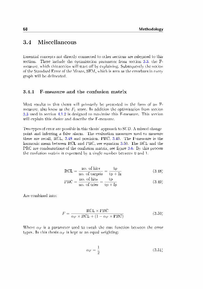
68 Methodology
3.4 Miscellaneous
Essential concepts not directly connected to other sections are relegated to thissection. These include the optimisation parameter from section 3.3, the F-measure, which this section will start o� by explaining. Subsequently the notionof the Standard Error of the Means, SEM, which is seen as the errorbars in everygraph will be delineated.
3.4.1 F-measure and the confusion matrix
Most results in this thesis will primarily be presented in the form of an F-measure, also know as the F1 score. In addition the optimisation from section3.3 used in section 4.1.2 is designed to maximise this F-measure. This sectionwill explain this choice and describe the F-measure.
Two types of error are possible in this thesis' approach to SCD. A missed change-point and inferring a false alarm. The evaluation measures used to measurethese are recall, RCL, 3.48 and precision, PRC, 3.49. The F-measure is theharmonic mean between RCL and PRC, see equation 3.50. The RCL and thePRC are condensations of the confusion matrix, see �gure 3.6. By this processthe confusion matrix is expressed by a single number between 0 and 1.
RCL =no. of hits
no. of targets=
tptp + fn
(3.48)
PRC =no. of hitsno. of tries
=tp
tp + fp(3.49)
Are combined into:
F =RCL× PRC
αF × RCL + (1− αF × PRC)(3.50)
Where αF is a parameter used to tweak the cost function between the errortypes. In this thesis αF is kept at an equal weighting:
αF =1
2(3.51)

3.4 Miscellaneous 69
Figure 3.6: The confusion matrix. A graphical representation of the possibleoutcomes of any binary choice. For practical reasons the confusionmatrix, in the context of this thesis, is distilled into the precision3.49, the recall or sensitivity 3.48 and the speci�city 3.56. Theprecision and recall are then further distilled into the F-measure.While the sensitivity and the speci�city are used to generate ROCcurves.
This is done in order to maximise the F-measure, the option of tweaking thecost between errors is included in the code as some practical system may havea higher intolerance for either error type.
The primary advantage of the F-measure for this thesis, beyond the convenientsimpli�cation of the confusion matrix, is that it circumvents the need for aknown number of true negatives, tn, which in other words is the correct absenceof check. In the context of this thesis' approach to SCD, correct absence ofcheck is not applicable, see �gure 1.1.
A change-point proposed by the algorithm may not be precisely aligned withthe actual change-point. To take this into account, a found change is countedas correct if it is within 1 second of the correct change-point as de�ned by theTi parameter, see section 2.3.
The implementation of the F-measure is found in appendix A.6.1 and in thecontext of FAC in appendix A.4.3.

70 Methodology
Figure 3.7: This �gure elaborates on how the confusion matrix is applied in thecontext of FAC and in extension how PRC, RCL and F-measure�t. The di�erent cases show how the concepts of tp, fp, fn andtn apply to FAC choices. As seen from the color the examples aretaken from the K-means method, the blue curve therefore repre-sents the VQD metric. The green dotted line represents a truechange-point, with the absence denoting a non-change-point posi-tion in time. The magenta circles represent change-points markedas false alarms (a positive hypothesis) and the green circles denot-ing that the FAC algorithm rejected it as a false alarm (a negativehypothesis).
3.4.1.1 Interpretation of FAC performance
Both proofreaders found that the calculation of FAC performance was obscure,this section will try to shed light on this issue. Figure 3.7 shows the confusionmatrix and how the corresponding FAC cases �t into it.
Furthermore, when the various result sections conclude that FAC is used ag-gressively what is meant is that if:
RCL > PRC (3.52)tp
tp + fn>
tptp + fp
(3.53)
fn < fp (3.54)
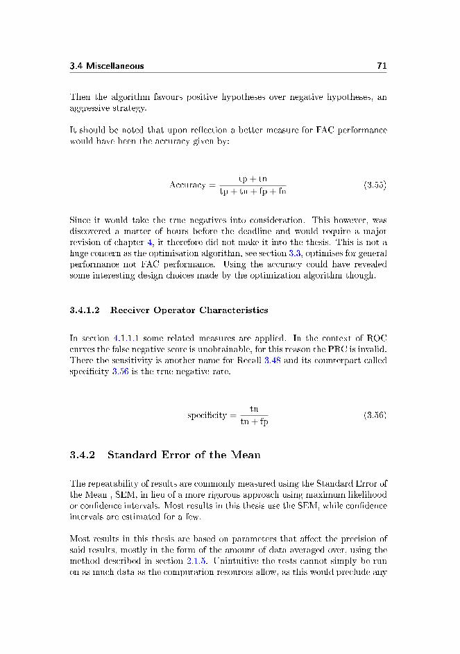
3.4 Miscellaneous 71
Then the algorithm favours positive hypotheses over negative hypotheses, anaggressive strategy.
It should be noted that upon re�ection a better measure for FAC performancewould have been the accuracy given by:
Accuracy =tp + tn
tp + tn + fp + fn(3.55)
Since it would take the true negatives into consideration. This however, wasdiscovered a matter of hours before the deadline and would require a majorrevision of chapter 4, it therefore did not make it into the thesis. This is not ahuge concern as the optimisation algorithm, see section 3.3, optimises for generalperformance not FAC performance. Using the accuracy could have revealedsome interesting design choices made by the optimization algorithm though.
3.4.1.2 Receiver Operator Characteristics
In section 4.1.1.1 some related measures are applied. In the context of ROCcurves the false negative score is unobtainable, for this reason the PRC is invalid.There the sensitivity is another name for Recall 3.48 and its counterpart calledspeci�city 3.56 is the true negative rate.
speci�city =tn
tn + fp(3.56)
3.4.2 Standard Error of the Mean
The repeatability of results are commonly measured using the Standard Error ofthe Mean , SEM, in lieu of a more rigorous approach using maximum likelihoodor con�dence intervals. Most results in this thesis use the SEM, while con�denceintervals are estimated for a few.
Most results in this thesis are based on parameters that a�ect the precision ofsaid results, mostly in the form of the amount of data averaged over, using themethod described in section 2.1.5. Unintuitive the tests cannot simply be runon as much data as the computation resources allow, as this would preclude any

72 Methodology
information on the precision of the result, beyond the knowledge that it is asprecise as possible.
To get a measure of the precision of a results; the result which itself is theaverage over results from data will have to be repeatedly gathered.
This is where the notion of SEM enters the picture. To avoid running severaltrials of the series of experiments averaged to get a result, the average of a seriesof experiments is assumed to be normally distributed. Using this assumption,the series of experiments only has to be run once and the accuracy of the averagecan be approximated [27]:
SEM =s√N
(3.57)
Where s is the standard deviation of results calculated using equation 3.10 andN is the number of results obtained.
The SEM of results are provided in the form of error bars in every graph.

Chapter 4
Application
This chapter will describe and discuss how the various methods are compared,contrasted, combined and improved. This is done by �rst performing individualfeature selection for the various methods using ROC curves based on the metrics,see �gure 3.1. ROC curves are used to enable pre-training feature selection ofthe methods, as it circumvents the entire change-point detection system, seesection 2.3.
Subsequently the remaining methods, along with a hybrid method, are trainedusing the novel optimisation technique, see section 3.3, the results of which arecompared based on the F-measure, the thoroughness and the e�ciency as ap-plied on test data. Evaluation of the involved trade-o�s are made and the KLmethod is shown to outperform the other methods. The KL method subse-quently undergoes a �nal backward feature selection based on a model of thehuman speech production system, see section 2.2.4. This backwards featureselection is shown to result in a marked increase in SCD performance.

74 Application
4.1 Feature selection and method comparison
This section starts with a pre-training comparison based on receiver operatingcharacteristic, ROC, curves which are used to perform forward feature selectionon the raw metrics without any FAC. In addition to this, the ROC curves areused to rule out DSD as a SCD metric due to its poor performance and they areused to determine a suitable codebook size for K-means, which is subsequentlyvalidated during training.
4.1.1 Pre-training method comparison
This section will describe how ROCs are generated and used as a precursor tomodel training for model choice elimination and feature selection.
The problem of comparing metrics is tricky as individual metrics may outper-form each other depending on the choice of basic parameters such as the varioustime constants, described in section 2.3, but may also outperform each otherdepending on the feature set used. This section will compare the use of �rstand second order derivatives of the MFCCs for the various metrics, moving for-ward with separate feature sets onto the post-training method comparison, seesection 4.1.3, as necessary. Once a �nal method is selected a backward featureselection will be performed, see section 4.3.1. As this project builds on the workof Jørgensen et al. [55], this section will use the basic parameters found to beoptimal previously, see section 2.2.
In order to compare the di�erent metrics a method is needed that can workwithout the entire change point selection mechanism, described in section 2.3,the reason being that this will eliminate a signi�cant amount of the parameterssimplifying the problem immensely.
Using this method it is unfortunately not possible to apply the FAC mechanismdescribed in section 2.4, the reason being that the iterative approach is incom-patible with the ROC method used here. Nonetheless the FAC mechanism onlyimproves the results slightly, see section 4.1.2.2.3, and the rough estimate ofmodel performance achieved using ROCs should su�ce.

4.1 Feature selection and method comparison 75
4.1.1.1 ROC generation
The method used to generate the ROCs was borrowed from the supervisor L.K. Hansen, see appendix A.6.4.
The method has been adapted slightly to improve the performance in the contextof this thesis, mainly the application of a non-constant threshold, this howeverwas achieved through manipulations of the input. The method in essence takesa metric and a list of equal length specifying when change-points occur as input.The change-points are de�ned as true if within Ti seconds, as described in section2.3.
The algorithm subsequently varies the gain on the moving average of the metricin order to scan over the ROC. The moving average de�nes the threshold, similarto what is described in section 2.3.
Ideally this method would simply scan the threshold over the metric calculatingthe precision and the speci�city for each iteration, enabling the use of FAC, seesection 2.4, however this would pose some key issues. The primary issue beingthat the change-point detection, the 1-dimensional peak detection algorithm,borrowed from [55] has the Ti constraint on the minimum distance betweenproposed change-points, in other words it is biased towards not predicting anexcess of change-points. This in essence would result in a ROC that does notconverge towards a ratio of one, instead the speci�city would converge to onewhereas the precision would converge to some value between 0 and 1 dependingon the size of Ti. This would not necessarily facilitate the comparison of di�erentmetrics.
To avoid this complication, at each iteration, the algorithm simply calculatesthe precision as the percentage of metric above the threshold within Ti secondsaround each change-point and calculates the speci�city in an identical mannerfor the parts of the metric not within Ti seconds of a change-point.
This method arguably is biased towards metrics with slow slopes around change-points, but is far more robust, does converge to a ratio of one and the steepnessof the slopes on the proposed metrics as roughly similar. This method willnaturally only evaluate the metrics abilities to model speaker change dynamicsat the used analysis window length of 3 seconds, borrowed from [55], see section2.3.
The more complex methods, K-means and RuLSIF, may be able to more closelyfollow the speaker change dynamics when given longer analysis windows, i.e.they would provide better performance in the context of FAC, see section 2.4.

76 Application
In actuality this method is performed through sorting lists of indexes as aniterative based approach would be time consuming.
4.1.1.2 Results from ROC analysis
Figure 4.2 shows an example of the metric scores with the actual change-pointsmark as the region contained by the vertical lines. Using the method describedin section 4.1.1.1 the ROC curves in �gure 4.2 are generated, using no MFCCderivatives, using only 1st and using both 1st and 2nd derivatives respectively.As all curves are smooth arcs the concept of Area Under the Curve, AUC,applies directly and is used to marginalise each curve to a single performancescore, see Figure 4.1, here the di�erent methods are compared to each other asa function of used derivatives.
As seen in �gure 4.1, DSD consistently under-performs all other methods. Inaddition the only theoretical di�erence between KL and DSD is whether or notthe mean of the normal distribution �tted to the data is discarded, which in thecase of DSD it is, see section 3.2.2.4. For this reason DSD as a change-detectionmethod is discarded.
Another interesting conclusion that can be drawn from �gure 4.1, is that DSDand KL improve performance with the addition of derivatives as features, whereasK-means signi�cantly decreases in performance. This K-means e�ect might becaused by the 'hub e�ect', discussed in section 4.1.1.3.3, a feature of the notfully understood curse of dimensionality [52]. How the size of K, number ofcentroids, a�ects the AUC is investigated in section 4.1.1.3.2, su�ce to say thata suitable value for K is found to be 25 in section 4.1.2.1. The use of derivativesdoes not appear to a�ect RuLSIF performance greatly, for convinience and tofacilitate the novel method described in section 2.4.1, the full feature set is usedfor RuLSIF.
Going forward with alpha training, see section 4.1.2, RuLSIF and KL will betrained using all features, that is 0th, 1st and 2nd derivatives, whereas K-meansis trained and designed to work on the smallest subset of the features to avoidthe derivatives issue, see section 4.1.1.3.3.
It should be mentioned that the use of 3rd derivatives and upwards are not testedfor two reasons. First, the ISP toolbox [53] does not support this and second,no mentioning of the use of higher derivatives has been found in the literature.This however might be interesting to investigate as the slope of KL seems toindicate that it will outperform the other methods using higher derivatives orpossibly just more features.

4.1 Feature selection and method comparison 77
Figure 4.1: This �gure displays the feature selection results from section4.1.1.2. All four methods were run using 1500 change-points, cor-responding to roughly 4 hours of speech, and every feature/methodcombination were run 2 times to verify the approximate repeata-bility. A ROC curve was then calculated for each point, see �guresin 4.2, and marginalised to their AUC. The errorbars represent thestandard error of the results.As seen the RuLSIF method in terms of AUC barely changes de-pending on the feature set applied. For convenience and to enableuse of the hybrid method between KL and RuLSIF, see section2.4.1, RuLSIF will use the full feature set.DSD and KL both show marked improvement using the largerdataset in spite of the dimensionality issue mention in section3.2.2.2. Since DSD shows signi�cantly worse results it is discardedfrom here on in.The K-means method on the other hand shows a marked decreasein performance with the larger feature sets, this is investigated indetail in section 4.1.1.3.

78 Application
Figure 4.2: This �gure serves as the example for the abstraction levels belowthe results seen in �gure 4.1.In (A) a 2 minute example of the about 4 hours of data for eachmetric in each trial is displayed for reference. Figures (B-D) arecalculated by varying a moving threshold of each metric seen in(A) for the feature set displayed in the titles of (B-D), as describedin section 4.1.1.1.

4.1 Feature selection and method comparison 79
It should also be mentioned that the use of more features in the form of deriva-tives does increase the overall likelihood of over-�tting, see section 3.2.2.2.
4.1.1.3 K-means - Feature and codebook size selection
As mentioned in section 4.1.1.2, a trade-o� between the dimensionality of thefeature vector and the amount of centroids, K, must be explored for K-meansto be an e�ective method. This section will explore this trade-o� and make asuitable selection for use in alpha training, see section 4.1.2.
This section will scan over a range of K, using the ROC method described insection 4.1.1.1, for three choices of feature sets, these being without derivatives,with 1st derivatives and with 1st & 2nd derivatives. Initially the values of K arespaces logarithmically in the suitable range, from 1 centroid to about a centroidfor every 2 data points. Since a singleton approach is taken to empty clustersin the version of K-means applied here, see section 3.2.1.2, as K approaches thenumber of data points in an analysis window the K-means method begins toresemble some version of a nearest neighbour metric [8], such an approach couldbe taken, but is not investigated in this thesis.
Going into this section the hypothesis was that the de�ciency of K-means withincreasing derivatives, found in section 4.1.1.2, was attributed to some versionof the 'hub problem', see section 4.1.1.3.3. In essence this would mean that asuitable choice of K should merely di�er depending on the input feature space.However as seen in �gure 4.3, the choice of K is not su�cient to account forthe decrease in AUC. In e�ect this might still be caused by some dimensionalityissue, however no means to compensate for it remains as the value of K is theonly free parameter in the Euclidean distance based K-means algorithm, seesection 3.2.1.2.
The de�ciency could be caused by the optimisations described in section 3.2.1.4,this however has not been tested since the simulation would take signi�cantlylonger without these optimisations.
Another interesting point is that given a single centroid the K-means algorithmreduces to a geometric mean distance metric. This approach in combination withthe DSD measure would resemble the KL distance, what is interesting to noteis that DSD and K-means with K=1 both have an AUC of approximately 0.89.The fact that the KL measure has an AUC of about 0.92, means that they encodecomplimentary information, giving yet another reason for the invalidation of theDSD metric as a method for SCD. It should be noted that this work does notexplore which parts of the auditory information is carried by the covariance and

80 Application
Figure 4.3: Performance of K-means as a function of codebook size for di�er-ent sets of MFCCs. Each set is comprised of derivatives of the12 MFCCs as described in section 2.2. Each combination is re-peated 10 times using a random set of 100 change-points drawnas described in section 2.1.5. The error bars indicate the standarderror, described in section 3.4.2, under the assumption that themean is drawn from an underlying normal distribution. The per-formance is measured using the AUC measure calculated using theROC method described in section 4.1.1.2. As seen the performancedeteriorates with the addition of more derivatives irrespective ofcodebook size, this may merely be caused by the increasing di-mensionality, as discussed in section 4.1.1.3.3. The peak at K=27is shown in greater detail in �gure 4.4.

4.1 Feature selection and method comparison 81
which is carried by the mean, it might be of interest to discard one of themgiven that the other might base the SCD decision on more reliable information,see section 3.2.2.4.
4.1.1.3.1 Feature selection
Going forward with alpha training, see section 4.1.2, the K-means method willbe trained without the use of the derivatives of the input features. The reasonbeing that �gure 4.3 shows a signi�cant advantage irrespective of the number ofcentroids. Whether K-means is merely under-performing for higher dimensionalspaces irrespective of the number of centroids would need further analysis. Thisfurther analysis could be in the form of a comparison between the performances,using various combinations of features, while keeping the absolute amount offeatures constant. This further analysis into an optimal feature set for this par-ticular method, K-means, would have been examined using backwards featureselection if K-means had proved to be the most viable method. As seen insection 4.1.3, KL proves to be a superior method in terms of a performance-e�ciency ratio, for this reason the backwards feature selection is performed onKL, see section 4.3.
4.1.1.3.2 Centroid amount selection
The work by Kinnunen et al. [61] concludes that identi�cation rate increaseswith increasing codebook size. Figure 4.3 however seems to indicate a peakaround K=27 using only the MFCCs. Using MFCC and 1st derivatives doesalso indicate this peak. In order to investigate this further the simulation isrerun at higher precision between the values K=20 to K=35 using only theMFCCs, see �gure 4.4.
Figure 4.4 obviously does not indicate any statistically signi�cant advantage ofone value of K over another K. To further illustrate this, �gure 4.5 shows theresults from the test run a second time.
The results here do not provide any reason to choose a speci�c value of K,beyond the need for it to be above about 10. Theoretical speculations in section3.2.1.2.1 indicate that a higher value of K may be preferable. However e�ciencyresults from section 4.1.3.2 indicate that K-means must be fairly optimised tobe of practical use. For these reasons K-means will be trained using the fairlyhigh value of K=56 chosen in [55] and the value of K=25, as �gure 4.4 doesindicate a peak. Whether the amount of centroids in�uence the performancecan be seen in section 4.1.2.1, where K=25 is compared to K=56.

82 Application
Figure 4.4: Figure 4.3 promted a more precise test around a codebook size ofK=27, the results of which are shown here. The results here showthat the peak around 27 was statistical noise. To further illustratethis point, this test is rerun in �gure 4.5, showing a completelydi�erent results. The test here is run 10 times and the errorbarsindicate the standard error.
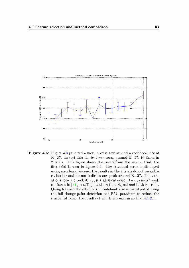
4.1 Feature selection and method comparison 83
Figure 4.5: Figure 4.3 promted a more precise test around a codebook size ofK=27. To test this the test was rerun around K=27, 10 times in2 trials. This �gure shows the result from the second trial, the�rst trial is seen in �gure 4.4. The standard error is displayedusing errorbars. As seen the results in the 2 trials do not resembleeachother and do not indicate any peak around K=27. The vari-ations seen are probably just statistical noise. An upwards trend,as shown in [61], is still possible in the original and both re-trials.Going forward the e�ect of the codebook size is investigated usingthe full change-point detection and FAC paradigm to reduce thestatistical noise, the results of which are seen in section 4.1.2.1.

84 Application
4.1.1.3.3 K-means and high dimensional data
Two hypotheses can be drawn from K-means failure when using derivatives,seen in section 4.1.1.2, either the derivatives hold very little information, whichthe results from the other metrics refute, or K-means has issues that do nota�ect the other methods. The reason that K-means fails using high dimensionaldata might be linked to the higher dimensionality of the input space usingderivatives, this is also discussed in section 4.1.1.2. If this is the case then oneof the reasons posted in a survey by Zimek et al. [126] where they identi�edthe following problems when searching for anomalies in high-dimensional datacould be the cause:
1. Concentration of scores and distances: derived values such as dis-tances become numerically similar.
2. Irrelevant attributes: in high dimensional data, a signi�cant amountof attributes may be irrelevant.
3. De�nition of reference sets: for local methods, reference sets are oftennearest-neighbour based.
4. Incomparable scores for di�erent dimensionalities: di�erent sub-spaces produce incomparable scores.
5. Interpretability of scores: the scores often no longer convey a semantic.meaning
6. Exponential search space: the search space can no longer be system-atically scanned.
7. Data snooping bias: given the large search space, for every desiredsigni�cance an hypothesis can be found.
8. Hubness: certain objects occur more frequent in neighbour lists thanothers.
In particular the Hubness might be an issue with respect to K-means. Partic-ularly as centroids would gravitate towards these meaningless - in the contextof SCD - Hubs. In addition to this, point number 1 might pose problems forK-means as it is heavily based on distance measures. In this case an input spaceof higher dimensionality might render K-means more susceptible to noise, sincemaking distances more similar would decrease the signal to noise ratio.

4.1 Feature selection and method comparison 85
4.1.2 Method training results
Given that the ROC method - used to provide a rough comparison of the metrics,see section 4.1.1.2 - only succeeded in eliminating a single candidate. The fullmethod is trained using K-means, KL and RuLSIF as contenders. In additionthe results in section 4.1.1.2, prompted an idea for a novel FAC method, heretermed CMFAC, the concept behind this novel approach is described in section2.4.1. In this section CMFAC will be used to apply RuLSIF as FAC metricto KL, the result of which is compared to the pure methods that made it intothreshold training.
The choice of codebook size for K-means proved ambiguous in section 4.1.1.3.2;therefore this section will start o� by comparing two choices of codebook size,before moving on to compare K-means with KL, RuLSIF and the KL/RuLSIFhybrid. This codebook size comparison is on the basis of the F-measure at thelocal maxima of the cost-function that the individual codebook choices locatein the threshold parameter space. As well as on the relative magnitude betweenchosen thresholds for each method.
4.1.2.1 Compare K-means codebook sizes
The ROC method applied in section 4.1.1.3.2 was unable to select a codebooksize for K-means, as it appeared to reach a maximum around K = 20 withfurther increase having no statistically signi�cant impact.
Previous work found that larger codebook size should increase performance[55, 61] and the ROC method was deemed too coarse to discount the literature.For this reason the values of K=25 and K=56 were selected, K=25 was selectedas a probably statistically insigni�cant peak was located there, see �gure 4.4,and K=56 was chosen as that was the value chosen in [55].
This section will apply the full training method, described in section 3.3, tothese two values and compare the results. The results of this process can beseen in �gures 4.6 and 4.7 for K=25 and K=56 respectively.
As seen in �gures 4.6 and 4.7, the end results is identical to 3 signi�cant digits,both choosing an αcd around 1.1 and an αFAC around 0.91. The more expensivemethod using K=56, �gure 4.7, chose to favor FAC slightly more, but not toa signi�cant degree. The F-measures found for the di�erent approaches is alsoe�ectively identical meaning that the approaches probably found the same localmaxima, again lending credence to the hypothesis that the codebook size isirrelevant.

86 Application
Figure 4.6: This �gure shows the K-means algorithm trained using a code-book size of K=25, with the colours representing the F-measurefor the corresponding threshold gain combination, the contours inbetween is a linear interpolation.The ROC based method used in section 4.1.1.3 was unable to pro-vide an unambiguous answer to the question on whether a largercodebook size in the K-means algorithm would yield better results.The results seemed to indicate that an increase beyond K=25 hadno e�ect. This section tests this de�nitively by training the fullK-means algorithm on both K=25 and K=56, see �gure 4.7, usingthe optimisation method from section 3.3. As seen the results fromthe 2 trials using K=25 and K=56 show almost identical results.For this reason K=25 is used as it is more e�cient.

4.1 Feature selection and method comparison 87
Figure 4.7: This �gure shows the K-means algorithm trained using a code-book size of K=56, with the colours representing the F-measurefor the corresponding threshold gain combination, the contours inbetween is a linear interpolation.This �gure is the second part in the K-means codebook selectiontest. See �gure 4.6 or section 4.1.2.1 for further details.

88 Application
Obviously to get an unbiased result the found parameters should be used to runa series of test on the test data. E�ectively a hypothesis test is clearly needed to�nd any signi�cant di�erence between the results using di�erent codebook sizes.However, as the results are almost identical any di�erence would be insigni�cantcompared to the additional computational cost of the larger codebook.
For this reason the series of tests on test data are not performed as this would bea waste of resources. The parameters found using the smaller codebook (K=25)are selected and compared to the other contenders, KL and RuLSIF in section4.1.2.
4.1.2.2 Pre-test comparison
As the alpha training, see section 3.3, of the K-means algorithm was run insection 4.1.2.1, only the alpha training of the KL and RuLSIF metrics remain.The reader is reminded that DSD was discarded in section 4.1.1.2. This sectionwill therefore begin by providing the results for the remaining metrics, thensubsequently compare the 3 metrics on the basis of performance and e�ciencyusing as of yet unused test data. In addition to this the combination of KL andRuLSIF using CMFAC, see section 2.4.1, is trained and compared to the puremethods using standard FAC, see section 2.4.
4.1.2.2.1 Threshold training
The alpha training results of the KL and the RuLSIF metrics are displayedin �gure 4.8 and �gure 4.9 respectively. The result for the KL/RuLSIF combi-nation using CMFAC, see section 2.4.1, is shown in �gure 4.10.
In �gure 4.8 the result of the threshold training for the KL metric is displayed.As the KL metric is quite light computationally, see section 4.1.3.2, a large res-olution along with a large amount of data per threshold combination is possible.What is interesting to note is that the strength of the grid search is very evidenthere. In �gure 4.8 top left the overall envelope of the cost function appears tohave two minima (or maxima in F-measure). In the second iteration using moredata, top right, this however turns out to be random �uctuations as one simplyturns out to be an upwards slope.
As seen in �gure 4.9 the process did not completely follow the procedure de-scribed in section 3.3. As the RuLSIF method proved too computationally heavyto fully realise the process. Only relatively few change-points are used for eachcombination and the resolution of each iteration is set to a bare minimum. As

4.1 Feature selection and method comparison 89
Figure 4.8: The colours - which are a linear interpolation of the values of thegrid - represent the F-measure for the corresponding thresholdgain combination. Note that the grid is independent of the axes.This �gure displays the training steps and training result of the fullKL method; using the optimisation method described in section3.3, the results here are compared to the other methods on trainingdata in table 4.1. The various methods are compared using testdata in section 4.1.3.As seen in this �gure a large amount of data is drawn for eachgrid point, and the resulting objective function is very smooth. Inthe �rst iteration the grid method �nds two peaks and selects oneof them, in the second iteration using more data it realises thatthere really was only a single peak.

90 Application
Figure 4.9: The colours - which are a linear interpolation of the values of thegrid - represent the F-measure for the corresponding thresholdgain combination. Note that the grid is independent of the axes.This �gure displays the training steps and training result of thefull RuLSIF method; using a slightly scaled down version of theoptimisation method described in section 3.3. As seen the reso-lution is kept at a bare minimum and the data amount is quitelow, yet still running the 3rd iteration and the �nal direct searchmethod proved too computationally expensive. The results hereare compared to the other methods on training data in table 4.1.The various methods are compared using test data in section 4.1.3.As seen the envelope of the cost function appears relatively smoothand the maxima found in the �rst iteration is also located in thesecond iteration indicating that the algorithm is probably center-ing on a maxima and not just on noise.

4.1 Feature selection and method comparison 91
such only the �rst step is ful�lled, namely locating the approximate maximaof the cost function envelope. The second step of locating a local maxima ofthe �ne structure and the �nal step using a non-linear optimisation algorithmwas skipped as this process would take on the order of weeks to �nish. As seenthe envelope of the cost function appears relatively smooth and the maximafound in the �rst iteration is also located in the second iteration indicating thatthe algorithm is probably centring on a maxima and not just on noise. Thethreshold gains could clearly be optimised further probably yielding an increasein F-measure of no more than about 0.01 � 0.02. RuLSIF might have bene�tedfrom a training session without FAC altogether, see section 2.4, thereby locatingthe precise peak of the local maxima seen in the �gure on the left on the southborder, as the computing power could then be concentrated on a 1-dimensionalgrid-search rather than a 2-dimensional one. This test was not performed as itwould require unavailable computing resources. It should be mentioned that aFAC'less approach is provided for reference using KL in section 4.1.2.2.3, show-ing a fairly marked lose in performance.
It should be mentioned that the missing square, in the top right corner of �g-ure 4.9, merely indicates that no change-points at all were found given thatparameter combination.
The results for the CMFAC metric combination using KL and RuLSIF is shownin �gure 4.10. As seen in section 4.1.3.2, the cost of applying the computationallyheavy RuLSIF even as a FAC step signi�cantly decreases the computationale�ciency, for this reason the data applied for each threshold combination is setquite low to keep the resolution high. This trade-o� was selected to make surethe global maxima was not simply too narrow to be missed and since the processyields fairly consistent results, as seen in the smoothness of the cost-function.
What is shown in this training session is quite interesting; the south border witha threshold gain of 2 on the CMFAC RuLSIF metric was found heuristically tobe the point at which the CMFAC process had no e�ect at all, however as seenthe grid search method iteratively approaches this boundary even selecting avalue on it.
The obvious conclusion is that the CMFAC process failed completely, that thechange-detection is clearly better o� without it. Upon closer inspection thishowever is not the case, as the �nal local minima of the cost function yields anF-measure of comparable magnitude, if not larger, than the pure KL methodin �gure 4.8. Further, in section 4.1.2.2.3, the KL metric is trained withoutany FAC at all, this is shown to yield signi�cantly poorer results con�rming thenecessity for the FAC step.
The next natural conclusion is that this lower border of 2 is too high, that given

92 Application
Figure 4.10: The colours - which are a linear interpolation of the values of thegrid - represent the F-measure for the corresponding thresholdgain combination. Note that the grid is independent of the axes.This �gure displays the training steps and training result of theKL/RuLSIF hybrid method; see section 2.4.1, using the optimi-sation method described in section 3.3, the results here are com-pared to the other methods on training data in table 4.1. Thevarious methods are compared using test data in section 4.1.3.As seen the added RuLSIF FAC step to the very e�cient KLchange-point detection took its toll and the training was com-pleted using a fairly low amount of data per threshold gain com-bination.Interestingly this �gure shows that the hybrid method �nds anoptimal solution using a very high thresholds on both change-point detection and a very low threshold on FAC. Yet still man-ages to �nd a solution that seems as good, if not better than thepure KL method. This indicates that the CMFAC method usingRuLSIF is very pro�cient at locating very di�cult false alarms,but fails at locating false alarms that the pure method excels at.

4.1 Feature selection and method comparison 93
Table 4.1: This table shows the �nal threshold parameters for the variousmethods along with their results as applied on training data. Theintermediate stages, of the optimisation method, for the variousmethods can be seen in �gures, 4.8 (KL), 4.9 (RuLSIF), 4.6 (K-means) and 4.10 (the KL/RuLSIF hybrid). These results seem toindicate that as expected the more expensive methods pull slightlyahead of the more e�cient methods. The generalisability of theseresults are investigated in section 4.1.3.
the opportunity the algorithm would choose an even lower threshold gain onCMFAC. This step was rerun and a border of 2 was found to be very slightlytoo constricting, but was con�rmed to be suitable. The suitability is also seenin the path of the Nelder-Mead method, which is not designed to be constrainedby the boundaries of the grid search algorithm, yet decides to move slightlynorthward of the border.
4.1.2.2.2 Threshold training results
As seen in �gures 4.6, 4.8, 4.9 and 4.10 the threshold gains and the F-measuresfound in the training session are as seen in table 4.1.
The training results, seen in table 4.1, indicates a fairly close run between thedi�erent approaches. The results indicate that the most expensive method, RuL-SIF, is probably also the most precise given adequate computational resourcesfor the training process, which were unavailable.
As it stands K-means and RuLSIF show fairly identical results edging slightlyahead of the computationally cheapest and simplest solution, KL, and the ex-perimental KL/RuLSIF combination, which also yield similar results.
The results also show that the metrics di�er in SNR, as is also evident in �gure3.1. This di�erence in SNR is seen in the ratio between αcd and αFAC . Itis seen that K-means looks similar on the short time scale that the change-detection operates on to the long time scale of FAC. As is also seen in �gure3.1, KL shows a tendency to have a low noise �oor and a large di�erence in themagnitude of the peaks, this is seen to a�ect its performance as the change-

94 Application
detection threshold favors a large value and the smoothing long time scale ofFAC requires a much lower threshold. RuLSIF is somewhere in between thesetwo extremes, but su�ers from another unique disadvantage. For RuLSIF thenoise �oor is not independent of the speaker. This e�ect is seen visually in �gure3.1 and had impacts in section 4.1.1.1, where a moving average threshold hadto be employed, since otherwise the RuLSIF method falsely indicated a poorperformance.
The experimental KL/RuLSIF combination is oddly enough seen to favor avery restrictive change-detection step, apparently signifying that the CMFACRuLSIF step can correctly �lter out quite certain potential change-points asfalse alarms. It must be mentioned that K-means has an advantage given thatall the time-constants, see section 2.3, used in this thesis were borrowed fromthe previous project [55], which found the K-means method superior to the KLand DSD methods. In spite of this, section 4.1.3.2 will show that KL has itsadvantages. An optimisation of these time-constants could, as mentioned insection 4.1.1, not be performed until a method is selected and due to timeconstraints on the thesis are relegated to further work, see section 5. TheRuLSIF method was not applied in [54] as it was invented several years later[75].
These results are obviously not conclusive since they were the product of thetraining process, applied on training data. Section 4.1.3 will apply the met-rics with the optimised parameters on test-data, thus enabling a comparison inprecision, recall, thoroughness and e�ciency.
4.1.2.2.3 No FAC reference
In this section the KL metric is trained without the use of false alarm com-pensation, see section 2.4. This is not done as a viable method, but is meant asa reference to verify the necessity for the FAC step.
As the exclusion of the FAC step reduced the 2-dimensional optimisation to a 1-dimensional problem, the intricate multi-step optimisation procedure describedin section 3.3, is unnecessary. In 1-dimension the standard brute force approachis still computationally viable. The relevant range is simply split into a su�-ciently �ne resolution and the algorithm is trained with a large amount of datafor each individual potential threshold 10 times.
The result can be seen in �gure 4.11, displayed through the mean of the 10 runsalong with the corresponding SEM, see section 3.4.2.
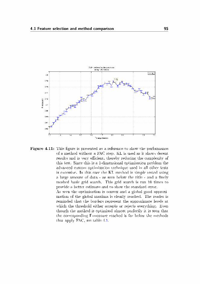
4.1 Feature selection and method comparison 95
Figure 4.11: This �gure is presented as a reference to show the performanceof a method without a FAC step. KL is used as it shows decentresults and is very e�cient, thereby reducing the complexity ofthis test. Since this is a 1-dimensional optimisation problem theadvanced custom optimisation technique used in all other testsis excessive. In this case the KL method is simple tested usinga large amount of data - as seen below the title - and a �nelymeshed basic grid search. This grid search is run 10 times toprovide a better estimate and to show the standard error.As seen the optimisation is convex and a global good approxi-mation of the global maxima is clearly reached. The reader isreminded that the borders represent the approximate levels atwhich the threshold either accepts or rejects everything. Eventhough the method is optimised almost perfectly it is seen thatthe corresponding F-measure reached is far below the methodsthat apply FAC, see table 4.1.

96 Application
As seen in �gure 4.11, the optimisation problem is quite simple. Clear slopesleading to a plateau with the algorithm selecting a threshold gain roughly inthe center of this plateau. The plateau is assumed to be a range of thresholdmagnitudes where a change merely shifts the precision-recall trade-o�. This as-sumption however remains untested as it is irrelevant to the actual optimisationsused.
Obviously the most important information this test yields is that the KL metricwithout the FAC step is signi�cant worse than with the FAC step. With anF-measure of 0.7786 compared to 0.8432 using FAC, see table 4.2. The othermethods have not been trained in a similarly rigorous fashion, but very imprecisetrial runs indicated that this conclusion holds for the other methods as well.
4.1.3 Post-test method comparison
This section will apply the remaining methods using the optimised thresholdparameters from section 4.1.2. The remaining methods are K-means, KL, andRuLSIF, since DSD was eliminated in section 4.1.1.2, along with the KL/RuL-SIF hybrid method.
This comparison will be on the basis of precision, recall, thoroughness and e�-ciency as applied on test data that was set aside for this purpose, see section 2.Finally this section will select a method based on this comparison.
In section 4.3.1, this chosen method will then be used to test the hypothesis thathigh MFCCs encode person speci�c information. In addition to this, the furtherwork section will apply various approaches to optimise this method further, thiswill however not be in a rigorous fashion and is meant to inspire further research,see section 5.
It should be mentioned that it would be interesting to compare the methodson the basis on how close the average potential change-point is to the truechange-point, as was done by Jørgensen et al. [55]. This however was foundto be very tricky as it required guessing to which true change-point a speci�cpotential change-point belonged. This was probably not a problem in [55] asa preprocessing step similar to the one described in section 2.1.4, was not per-formed. This left their data biased, but enabled model comparison on the basison change-point accuracy. For this reason, this particular comparison is notperformed and will not in�uence the choice of method.

4.1 Feature selection and method comparison 97
Table 4.2: The precise results of the method performance comparison. Fora more detailed description of the results and the implications see�gure 4.12 or section 4.1.3.1.
4.1.3.1 Performance results
Each method is run on a sample size of 500 change-points, or the equivalent ofabout 2 hours of speech, created using the method described in section 2.1.5.This is then repeated in a loop for each method individually with a runtime ofapproximately 10-12 hours per method. Depending on the runtimes, see section4.1.3.2, this resulted in somewhere between 8 and 68 reruns. The results arepresented in �gure 4.12 and table 4.2, with the error bars naturally representingthe SEM of the measurement. The corresponding FAC performance is seen in�gure 4.13 and table 4.3.
The reader is reminded that precision is the percentage of correctly placedchange-points, recall is the percentage of change-points found and the F-measureis the harmonic mean of precision and recall, see section 3.4.1.
From �gure 4.12 and table 4.2 it is seen that the performance of the methodshave shifted compared to each other when compared with training results, seetable 4.1. This is caused in part by the generalisation error, but is thought tomainly be caused by the selection of positive noise during training. This canbe seen in the fact that the generalisation error is inversely correlated with theamount of data used during the training procedure. Even though this correlationwould also cause a larger generalisation error, it is believed that this should notbe at this large a magnitude.
As seen the hybrid method su�ers the worst, whereas standard KL barelychanges at all. With the greatly reduced e�ciency of applying CMFAC, the onlyadvantage is in how well CMFAC does at identifying the tough false alarms, asmentioned in section 4.1.2. Interestingly this might merit a hybrid between thestandard KL and the Hybrid method using CMFAC, whereby both standardFAC and CMFAC is applied to KL in a similar fashion to the ensemble methodmentioned in section 2.4. The reason why this could increase performance is seenin table 4.1, where the CMFAC method chooses a very high change-detectionthreshold compared to standard FAC. In essence this means that the CMFAC

98 Application
Figure 4.12: The results from the method performance comparison using testdata in the form of an F-measure and is constituents. Eachmethod is run on a sample size of 500 change-points, created us-ing the method described in section 2.1.5. This is then repeatedin a loop for approximately 10-12 hours per method. Dependingon the runtimes, see section 4.1.3.2, this resulted in somewherebetween 8 and 68 reruns. For the precise numbers see table 4.2.Oddly enough the failures of the expensive metrics seem to out-weigh their bene�ts and the simple KL method seems to outper-form them using the current methodology. Not strictly in termsof F-measure - where K-means is slightly higher - but in terms ofa performance versus e�ciency ratio, see section 4.1.3.2. In ad-dition the KL method �elds the best recall score of all the meth-ods, indicating that it has the highest potential to see furtherimprovements, performed in section 4.3 and 5.2. This result iscounter-intuitive as the expectation was that the more advancedmethods would also have the highest potential. Their ine�ciencyduring optimisation shows through clearly.

4.1 Feature selection and method comparison 99
is optimised to only remove the tough false alarms, the ones standard KL willobviously tend to miss. This would also barely decrease e�ciency of the CM-FAC method as the standard KL FAC is very e�cient using less than 1% of thecomputing resources, see section 4.1.3.2. The task of implementing this ensem-ble base FAC is unfortunately beyond the scope of this thesis and is relegatedto further work, see section 5.
RuLSIF generalises poorly, probably due the poor training, this could undoubt-edly be improved by running the training algorithm of RuLSIF at a higherresolution. However as mentioned in section 4.1.2 and seen in section 4.1.3.2,this is not computationally feasible as such a simulation would take weeks if notmonths. It could be done using IMMs Cluster, however as mentioned in section3.3.1, that prospect has been exhausted. Therefore, due to the poor e�ciencyof RuLSIF it is not feasible in real world applications for years to come and isdiscarded as a change-detection method.
K-means fared slightly better than RuLSIF in the generalisation and actuallyshowed better results than all other approaches. The margin is slight as com-pared to standard KL and at the additional factor 2.5 increase in computa-tional runtime, see section 4.1.3.2, the better F-measure performance is clearlynot enough. Another point where K-means excels is in its precision where itonly competes with the hybrid KL/RuLSIF CMFAC method. Unfortunatelythis precision comes at the cost of a lower recall score, this is thought to becaused by the smaller feature space used by K-means, see section 4.1.1.3.1. Theconclusion is that K-means is a decent choice, but is upper bounded by itsdimensionality issues, see section 4.1.1.3.3.
Oddly enough the failures of the expensive metrics seem to outweigh their ben-e�ts and the simple KL method seems to outperform them using the currentmethodology. In addition the KL method �elds the best recall score of all themethods, indicating that it has the highest potential to see further improve-ments, performed in section 4.3 and 5.2. This result is counter-intuitive as theexpectation was that the more advanced methods would also have the highestpotential.
In �gure 4.13 and table 4.3, the FAC performance for the various methodsis seen. It is immediately obvious that the optimisation step tend to use FACaggressively, since it favors recall over precision, or in other words it has found itoptimal to remove potential change-point if they might be false alarms. Anotherinteresting note is that, as seen in �gure 3.1, RuLSIF as applied to speechdetects many 'changes' that do not correspond to speaker changes. What thesecorrespond to is untested, but this has shaped a method that relies heavily onFAC for SCD. However even though RuLSIF relies heavily on FAC, see table4.3 and �gure 4.14, it is simultaneously seen to spend very few computational

100 Application
Figure 4.13: The FAC performance during the method performance compar-ison, see �gure 4.12. As seen the optimisation step tends touse FAC aggressively, since it favours recall over precision. Inother words it has found it optimal to remove potential change-point if they might be false alarms. Interestingly it is seen thatstandard FAC for KL has almost the same recall as the CM-FAC method, but as expected the more expensive CMFAC issubstantially more precise. RuLSIF is seen to have the worstFAC performance, this however is misleading. As seen in �gure4.14 RuLSIF applied FAC to a far greater degree than the othermethods, it is actively using it, rather than merely polishing itsresults. Unsurprisingly the K-means method has a solid FACperformance in line with its great performance in general.
Table 4.3: The precise results of the FAC performance, see �gure 4.13, and thefalse alarm percentage, see �gure 4.14. For an explanation of theresults and their implications see the caption of the corresponding�gure or section 4.1.3.1.

4.1 Feature selection and method comparison 101
Figure 4.14: The false alarm percentage used by the methods during themethod performance comparison, see �gure 4.12. As seen RuL-SIF relies heavily on FAC, further decreasing its e�ciency, ithowever is simultaneously seen to spend very few computationalresources on the FAC step, see section 4.1.3.2. A discussion ofthis strange phenomena is found in section 4.1.3.1. The hybridmethod is seen to use FAC aggressively, which is fortunate asthat increases its e�ciency. It does however suggest that the hy-brid method fails to use FAC pro�ciently. K-means and standardKL are seen to use FAC in a more well-rounded manner. For theprecise percentages see table 4.3.

102 Application
Table 4.4: The precise results for the runtime test, included for reference. Fora description and interpretation of these results see �gure 4.15 orsection 4.1.3.2.
resources on the FAC step, see in section 4.1.3.2. The hypothesis is that thisis caused by a combination of factors; RuLSIF is optimised to produce a lot ofpotential change-points and then to remove these by applying FAC, this is seenin the relatively close threshold gains, see table 4.1. However with the largenumber of change-points the average distance between change-points decreases.During FAC the amount of data used to test for false alarms is maximised, butis limited to not use data within 1 second of other potential change-points, seesection 2.4. Since RuLSIF's runtime scales super-linearly with the data amountthe large number of change points might actually reduce the runtime of the FACstep.
It must be stressed though that this is an untested hypothesis and that itstesting is left to further work, see section 5.
If this is true, it would mean that RuLSIF might fare better on data withlong speaker turns, with a recursive FAC paradigm or without FAC entirely.However as RuLSIF is very computationally expensive none of these optionsare explored, the slight improvement in performance is far out weighted by thefurther decreases in e�ciency they would cost. This could potentially also bethe reason for the peak on the south border of left �gure in �gure 4.9, which isthe part of the function-space that corresponds to a FAC'less method.
It should be noted that RFAC is found to improve KL performance, see section5.2, and KL is found to decrease in performance without the FAC step, seesection 4.1.2.2.3. How/if this applies to RuLSIF is untested.
4.1.3.2 E�ciency results
Runtime measurements for the individual methods are displayed in �gure 4.15.
The time measure is a sum of the time it takes to calculate the models, the time

4.1 Feature selection and method comparison 103
Figure 4.15: The runtimes for the various method, displayed as the timeneeded per actual change-point, meaning that thorough meth-ods automatically score slightly higher. The data is presented ona logarithmic scale to �t all results onto the �gure, the precisenumbers are seen in table 4.4.As seen RuLSIF is very computationally heavy at about 2 or-ders of magnitude slower than the most e�cient method whichas expected is KL. This is also seen in the hybrid method, wherethe FAC step takes the majority of the computational e�ort. K-means has undergone several optimisations, see section 3.2.1.4,and is therefore faster than the hybrid, but still clocks in at 2.5times slower than KL.

104 Application
it takes to calculate the dissimilarity measures and �nally the time it takes torun the FAC. This sum is then normalized by the amount of change-points inthe measurement. It must be noted that the result here does not include theoverhead, e.g. the feature extraction among others. The result is presented asthe mean and the SEM. As seen in �gure 4.15, RuLSIF is very computationallyheavy at about 2 orders of magnitude, or more precisely 80 times, slower thanthe most e�cient method which as expected is KL.
K-means has undergone several optimisations, see section 3.2.1.4, and clocks inat 2.5 times slower than KL. The precise numbers are seen in table 4.4.
Disclaimer: It must be noted that the run-times are merely guidelines and theexact numbers depend on the implementation, particularly on how parallelizableit is and how well the MATLAB's Just-In Time, JIT, accelerator can optimiseit. The run times at measured using MATLAB's tic/toc functions.
To maintain a clean measure of the run-times the methods were naturally runindividually except for RuLSIF, which was run in parallel with itself to maximiseCPU usage. This slightly exaggerates is e�ciency, but was necessary to reducethe required total runtime.
For reference; the hardware used was a single Intel R© CoreTM i5-2400k proces-sor running four cores at 3.4GHz, 32GB RAM and running MATLAB 7.11.0(R2010b) 64-bit.
As such these run-time ratios are meant as guidelines, especially in the context ofimplementation outside the MATLAB environment, they are however assumedto be similar in such a case.
4.2 Method comparison conclusion
In summary the choice of applying K-means in the previous project by Jørgensenet al. [55] was a decent choice given the implementation. However it is foundin section 4.1.2.1, that a smaller codebook will increase e�ciency with no e�ecton the performance. The K-means method has a severe limitation though, itsperformance is upper bounded by its dimensionality issues, see section 4.1.1.3.3.
It is found here that the KL method is fairly unambiguously the superior methoddue to its close second in F-measure, its low computational cost and its highrecall indicating hidden potential. Furthermore the KL training procedure ise�cient enough that retraining given new data in commercial software is still

4.3 Method re�nement 105
slow, but not excessively so.
The backwards feature selection mentioned in section 2.2.4, will be performedon KL in section 4.3.1. Once an optimal feature set is found the KL methodwill undergo yet another training session, in section 5.2, using the multi-stepFAC method, mentioned in section 2.4.
4.3 Method re�nement
This section will test the hypothesis from section 2.2.4, that using only theupper MFCCs will improve performance. The theory is that the deconvolutionof the time signal via the ceptrum shifts the envelope of the spectrum to thelow MFCCs and the �ne structure to the high MFCCs. The hypothesis is thatthe human speech system when talking can be modelled as an Linear Time-Invariant, LTI, system with the excitation signal generated by the voice boxundergoing a convolution by the vocal tract acting as a linear �lter. The vocaltract �lter in this model shapes the excitation signal, thereby forming the literalsemantics of the speech signal, whereas the excitation signal is arbitrary, personspeci�c and should thereby work as sort of an acoustic �ngerprint.
4.3.1 Backwards feature selection
If the hypothesis from introduction to this section holds then the upper MFCCsshould yield better results than the lower MFCCs in the context of SCD. Thissection will use the designed optimisation tools from section 3.3 on the methodselected in section 4.1.3 to test this hypothesis. As mentioned in section 2.2.2,up till this point 12 MFCCs have been used along with their 1st and 2nd orderderivatives, in this section this will still be the case. What is changed is the Mel�lter bank size described in section 2.2.4.2.
As mentioned in section 2.2.1, 20 Mel �lters will be used and KL is trained onthe outputs of the 12 upper and on the 12 lower ones. The very �rst componentis obviously still left out, see section 2.2.2 for the explanation.
It must be noted that the ISP toolbox [53] - used to generate the MFCCs - doesnot support the selection of speci�c MFCCs. The ISP toolbox automaticallyselects the lower MFCCs, which probably means that it was designed with speechtranscription as the main focus. So far the outputs from all �lters have beenused; this has therefore not had an impact up till this point. At least that was

106 Application
the assumption, however - as described in the next paragraph - this was not thecase.
To enable feature selection the ISP toolbox [53] underwent more custom modi-�cations, see section 1.2. During this overhaul of the ISP toolbox, some leftoverdebugging code from its creation was discovered, wherein several inputs wereoverridden by custom, non-default values, in a fashion easily overlooked undera casual inspection and invisible from the outside. This included the amount of�lters used in the Mel �lter bank. This debugging code was obviously removedand all previous tests were scrapped and rerun. The creators of the ISP toolboxwere noti�ed and the entire toolbox was thoroughly examined. The relevantmodi�ed scripts can be seen in appendix A.5.4.
4.3.2 Training results
The training results of the KL method using the upper and lower MFCCs areshown in �gure 4.16 and 4.17, respectively. The training or optimisation methodused is described in section 3.3.
At a casual glance the results in �gures 4.16 and 4.17 seem similar; in bothcases the optimisation of KL is roughly a convex optimisation problem whichthe optimisation algorithm handles well. The results seem similar with themain di�erence being slightly steeper slopes in the upper MFCCs case. Howeverwhen studying the F-measures that the color contours correspond to and theF-measure at the found local minima the di�erence becomes readily apparent.
An interesting note is that the full KL method training results, see �gure 4.8,did show two peaks. While the upper and lower KL methods �nd one peakeach, see �gures 4.16 and 4.17. These original peaks might correspond to paireddown versions of the full method that resemble the upper and lower methods.Testing this hypothesis would however require an extensive feature selectionprocess which will not be performed.
In table 4.5 the training result using the upper and lower MFCCs are comparedto the previous training results using all MFCCs from section 4.1.2.
As seen in table 4.5, interestingly the FAC is apparently much more reliable inboth the lower and upper case compared to the full case, as the optimisationchooses to use signi�cantly more of it, especially the lower case which removesone out of four potential change-points, see table 4.3.
The fact that the algorithm is more FAC reliant means that it is better able

4.3 Method re�nement 107
Figure 4.16: The colours - which are a linear interpolation of the values of thegrid - represent the F-measure for the corresponding thresholdgain combination. Note that the grid is independent of the axes.This �gure displays the training steps and training result of theKL method using only upper MFFCs; using the optimisationmethod described in section 3.3. The results here are comparedto the other methods, all MFCCs and lower MFCCs, on trainingdata in table 4.5. The various methods are compared using testdata in section 4.3.3.As seen in this �gure a large amount of data is drawn for eachgrid point, and the resulting objective function is very smooth.In the �rst iteration the grid method �nds the global maximaroughly, the subsequent iterations and the direct search methodmerely locate the peak with greater precision.

108 Application
Figure 4.17: The colours - which are a linear interpolation of the values of thegrid - represent the F-measure for the corresponding thresholdgain combination. Note that the grid is independent of the axes.This �gure displays the training steps and training result of theKL method using only lower MFFCs; using the optimisationmethod described in section 3.3. The results here are comparedto the other methods, all MFCCs and upper MFCCs, on trainingdata in table 4.5. The various methods are compared using testdata in section 4.3.3.As seen in this �gure a large amount of data is drawn for eachgrid point, and the resulting objective function is very smooth.In the �rst iteration the grid method �nds the global maximaroughly, the subsequent iterations and the direct search methodmerely locate the peak with greater precision.

4.3 Method re�nement 109
Table 4.5: This table shows the �nal threshold parameters for KL using the3 feature sets, lower MFCCs, upper MFCCs and all MFCCs. Theintermediate stages, of the optimisation method, for the variousmethods can be seen in �gures, 4.8 (Full), 4.16 (upper) and 4.17(lower).Firstly it is seen that using the upper MFCCs, as expected, seemsto result in a marked improvement. Beyond this it is seen that theFAC is interestingly much more reliable in both the lower and uppercase compared to the full case, as the optimisation chooses to usesigni�cantly more of it, especially the lower case which removes oneout of four potential change-points, see table 4.3. It is believed thatthis is a re�ection of what a uni-modal model is able to interpret,see section 4.3.2.
to distinguish speakers given large amounts of data. As both K-means, butespecially RuLSIF applied more FAC than KL, see section 4.1.3, indicates thatthe lower and upper MFCCs distinguish speakers based on di�erent aspectsand that they were better able to model this bi-modal underlying PDF. Thisis as expected since RuLSIF and K-means do not model the speaker using auni-modal model like KL.
Interestingly this bodes well for KL as it should do well only looking at thelower or only the upper MFCCs. This is also indicated by the magnitude of theF-measure at the local minima found during training, see table 4.1; the trainingresult indicates that KL using lower MFCCs is almost as good as using the fullrange, however as the hypothesis this section set out to test states, KL usingonly the upper MFCCs shows great promise.
These results are naturally not conclusive as they are the product of the train-ing process, applied on training data. Section 4.3.3 will apply KL with therelevant feature set and the optimised parameters on test-data, thus testing thegeneralisability of the results found here.

110 Application
Figure 4.18: This �gure shows the performance of the upper and lower MFCCKL methods compared to the methods tested in section 4.1.3.1.The result is seen to be conclusive; compared to the previousfull range KL method, using only the upper MFCCs signi�cantlyimproves the performance, whereas using only the lower MFCCssigni�cantly deteriorates the performance. Where the full rangeKL lies in between, which further points to the hypothesis; thathigh and low MFCCs distinguish speakers di�erently and thatfull range KL being uni-model fails to capture each attributeindependently. Con�rming the validity of the speech productionsystem model from section 2.2.4.
4.3.3 Test results
In this section the test results for KL using lower MFCCs and using upperMFCCs are compared to KL using the full range, see section 4.1.3.
In �gure 4.18 and table 4.6 it is again con�rmed, as was seen in section 4.1.3,that the training result found using the optimisation method generalises verywell using the resolution and data amount applied here. The reader is remindedthat the reason why all methods tend to favor precision over recall is the directconsequence of the FAC paradigm. Furthermore the result is seen to be con-clusive; using only the upper MFCCs signi�cantly improves the performance,whereas using only the lower MFCCs signi�cantly deteriorates the performance.Where the full range KL lies in between which further points to the hypothesis;

4.3 Method re�nement 111
Table 4.6: The precise results of the method performance comparison betweenthe di�erent feature sets for the KL method. For a more detaileddescription of the results and the implications see �gure 4.18 orsection 4.3.3.
Table 4.7: The precise results of the FAC performance, see �gure 4.19, and thefalse alarm percentage, see �gure 4.20. For an explanation of theresults and their implications see the caption of the corresponding�gure or section 4.3.3.
that high and low MFCCs distinguish speakers di�erently and that full rangeKL being uni-model fails to capture each attribute independently.
In �gures 4.19, 4.20 and table 4.7, KL using the di�erent feature sets is comparedon the basis of FAC.
In �gure 4.19, 4.20 and table 4.7, the conclusion, from section 4.3.2, that KLwhen trained on lower or on upper MFCCs relies heavily on FAC is con�rmed.Similarly to the results with other methods in section 4.1.3, the FAC is erringon the aggressive side. It is also found that lower KL is far more reliant on FACthan upper KL, this seems to indicate one of two things. Either the informationrelevant for SCD in the lower MFCCs is found on fairly long time scales, at leastlonger than the analysis window size of 3 seconds or that lower MFCC is verysensitive to multiple speakers in an analysis window, something FAC inherentlycounteracts with its variable size analysis window, see section 2.4. Regardless ofthe reason for this KL using lower MFCCs is clearly inferior to KL using upperMFCCs. KL using upper MFCCs is seen to maintain the high recall FAC of fullrange KL, even though it applies FAC on twice as many potential change-pointsand has a greatly increased precision. This is clearly one of the reasons whyupper KL has superior performance compared to full range KL.

112 Application
Figure 4.19: This �gure displays the FAC performance during the performancetest for di�erent KL feature sets, see �gure 4.18, here comparedto the methods tested in section 4.1.3.1. Again the FAC methodis found to adopt an aggressive strategy - liable to throw awaypotential change-points if unsure - seen in the fact that RCL isgreater than PRC, see section 3.4.1.1. KL using upper MFCCs isseen to maintain the high recall of the full range KL, even thoughit applies FAC on twice as many potential change-points and hasa greatly increased precision. This is clearly one of the reasonswhy upper KL has superior performance compared to full rangeKL.

4.3 Method re�nement 113
Figure 4.20: This �gure displays the percentage of false alarms the KL methodchooses depending on the feature sets compared to all methodsfrom section 4.1.3.1. As seen the conclusion from section 4.3.2is con�rmed, the new KL methods rely choose to rely heavily onFAC. It is also found that lower KL is far more reliant on FACthan upper KL, this seems to indicate one of two things. Eitherthe information relevant for SCD in the lower MFCCs is found onfairly long time scales, at least longer than the analysis windowsize of 3 seconds or that lower MFCC is very sensitive to mul-tiple speakers in an analysis window, something FAC inherentlycounteracts with its variable size analysis window. This is notinvestigated as the lower MFCC method is clearly inferior to theupper MFCC one, see �gure 4.18.

114 Application
4.4 Method re�nement conclusion
In conclusion the hypothesis this section set out to test is clearly validated. KLshows marked improvement using only upper MFCCs compared to using thefull range, while maintaining the same feature vector size. Whereas using onlythe lower MFCCs forces the optimisation to choose a very heavy FAC strategy,however impressive this fails to reach even the performance of the full range KLfound to outperform other methods in section 4.1.3.
The impact of feature selection on the runtime of the KL method is left untested.The runtime would be slightly longer as both the lower MFCC and upper MFCCversions rely more on the FAC step than the full range MFCC version. Howeveras seen in section 4.1.3.2, this decrease in e�ciency would be very slight as theFAC step of the KL method is very e�cient, taking less than 1% of the fullruntime for the full-range MFCC version.
Doing a full backwards feature selection, rather than a single step as is performedin this section, seems very promising. However this would likely tune the methodto the format of the dataset and the generalisability could su�er; this howeverwould require the method be applied to other data sets than ELSDSR, which isbeyond the scope of this thesis. Beyond that a full backwards feature selectionwould be very computationally costly and though all the relevant software hasbeen created it is beyond the scope of this thesis to run it. The work hereunfortunately only has the resources to provide this proof of concept, the fullbackwards feature selection is left to further work, see section 5.

Chapter 5
Further work
Beyond the work described so far, a range of topics and �elds were propped andtested at varying degrees of rigorousness. This section will quickly describe theresults from the areas in which a su�ciently large amount of work was done.The methods and results presented in this section were not given adequateattention or computing resources to merit admission into the greater body ofwork. Beyond this, this section will conclude with a list of promising avenuesthat was left unexplored due to time constraints.
5.1 Speaker clustering
Once speaker change points have been identi�ed and the audio stream has beensegmented into a set of speaker turns, a crucial part of the original question of�who spoke when?� still remains, namely the who. Assuming some of the seg-ments are spoken by the same person, the task of identifying these and annotat-ing them with a label is an important part of speaker diarisation. As mentionedin section 1, this project does not attempt to classify these speech segments, theprocess of grouping the segments is purely addressed as a clustering problem.
This section assumes that the SCD process operates ideally separating speakersegments perfectly. The reason for this assumption is to avoid carrying over

116 Further work
biases from the SCD process. It must be noted that this assumption beyondrendering the process of perfect clustering ideally possible, removes the possi-bility of investigating possible non-linear processes whereby biases in the SCDprocess interact with biases in the clustering process.
By cluster, what is meant is that all MFCCs from a speaker segment are groupedtogether with sequential information ignored. The speaker clustering processuses the 12 MFCC 1st & 2nd derivatives upper range features found to improveresults in section 4.3.1.
5.1.1 Agglomerative Hierarchical Clustering
The clustering method implemented and compared in this thesis are variousdissimilarity measures using an Agglomerative Hierarchical Clustering, AHC,[8] approach. The basic concept behind AHC is to de�ne a dissimilarity metricto distinguish between clusters, e.g. the Euclidean distance between their clos-est members, usually in the form of linkage functions. Then to �nd the leastdissimilar clusters and combine them, repeating this process until some desiredcriteria is met.
This process is slightly more complicated when clusters cannot be directly com-pared in a geometric sense as is the case in this thesis. The reason being thateven using the process of MFC the clusters are occupying approximately thesame region of MFCC space, see �gure 2.2. This issue is dealt with by insteadof directly comparing clusters, a model with a set of parameters is trained todescribe the underlying cluster. This model is then compared to the modelstrained on every other cluster, forming the dissimilarity matrix, see an examplein �gure 5.1. This dissimilarity matrix must be computed fully at every step ofthe process, a range of method to optimise this was investigated, a good solutionwas not found.
This model comparison process brings with it an issue, as model training scalessuper-linearly with the data size. This issue is circumvented by simply buildingthe model on a random sample of the data. The size of this sample is set toTmax which all the way through this thesis has de�ned the maximal amount ofdata to be applied.
This sampling however brings yet another issue into the picture, which is thatsampled data might fail to represent the structure of the cluster. A solutionto this issue is proposed by Han et al. [42] in the form of a normalized BICbased dissimilarity measure termed the Information Change Rate, ICR. It iscalled ICR as [42] shows it measures how much information (entropy) would be

5.1 Speaker clustering 117
changed (increased) by merging the clusters under consideration. In this sense itfunctions slightly like a Kullback-Leibler dissimilarity metric with incorporatedregularization and normalization of cluster sizes.
Using the non-geometric dissimilarity measures enable AHC, but losses the sim-ple progression of ever more dissimilar cluster being the least dissimilar clusters,resulting in a slightly messy dendrogram. The issue of a non-simply progressionmakes the use of simple thresholding techniques as a stopping criteria fail.
The stopping criteria proposed here is to incorporate active learning techniquesincorporating the user of the audio editing software as an oracle. Settles [104]provides a broad view into the �eld of active learning. This framework of ideaswas not fully developed, but would require the user to provide an estimate ofthe amount of speakers in the pod-cast, the AHC algorithm would then look fora marked increase in dissimilarity around the required number of clusters.
5.1.2 AHC: Dissimilarity metrics
The AHC process is tested using all metrics described in section 3.2, alongwith the BIC and the ICR dissimilarity metrics as proposed in [42]. In thissection only the results from the KL trial, along with the BIC and ICR trialsare presented. The results are presented in the form of dendrograms, see �gures5.2, 5.3 and 5.4.
The generation of the dendrogram in �gures 5.2, 5.4 and 5.3, are repeated 5times and combined into the results seen in �gure 5.5.
In the top �gure in 5.5 it is seen that all metrics start mixing speakers into thesame clusters before all segments of the same speaker are combined. Resultingin a smooth transition to a single cluster containing all speakers. Beyond thisit is seen that BIC and KL do signi�cantly better at maintaining cluster puritythan ICR, as ICR start combing speaker clusters far in advanced of the targetvalue of 5 speaker clusters.
In �gures 5.2, 5.3 and 5.4, it is seen that the results from the KL and the BICapproach resemble each other and both work decently well. However a feed-backprocess is seen to deteriorates results. What happens is that two individuallyspeaker-pure clusters, of several speaker segments each, can resemble each othermore than the cluster's own outliers. When two of these pure clusters arecombined this process is even more likely to repeat itself, rapidly deterioratingthe results.

118 Further work
Figure 5.1: This �gure shows the dissimilarity matrix at a single step in theAHC process. As seen every segment is compared to every othersegment, this obviously forms a symmetric matrix, for e�ciencyonly one triangle is calculated. Segment dissimilarity is displayedthrough color, with deep blue being identical and deep red be-ing very dissimilar. The scale and slope of the dissimilarity isdetermined by the dissimilarity metric applied, in this case KL.As seen the dissimilarity matrix will form striped patterns, thisre�ects that some speakers are apparently very distinguishable.

5.1 Speaker clustering 119
Figure 5.2: This �gure shows the agglomerative hierarchical clustering processusing the BIC dissimilarity metric in the form of a dendrogram.As seen the algorithm does fairly well to begin with at combiningsegments spoken by the same person. What is however also seen isthat as soon as the process combines clusters containing di�erentspeakers a feed-back e�ect occurs, making more misclassi�cationmore likely. This feed-back e�ect makes the approach less appeal-ing. This is also evident using KL, but the results from the ICRtrials hints at a solution.

120 Further work
Figure 5.3: This �gure shows the agglomerative hierarchical clustering processusing the KL dissimilarity metric in the form of a dendrogram.As seen the algorithm does fairly well to begin with at combiningsegments spoken by the same person. What is however also seen isthat as soon as the process combines clusters containing di�erentspeakers a feed-back e�ect occurs, making more misclassi�cationmore likely. This feed-back e�ect makes the approach less appeal-ing. This is also evident using BIC, but the results from the ICRtrials hints at a solution.

5.1 Speaker clustering 121
Figure 5.4: This �gure shows the agglomerative hierarchical clustering processusing the ICR dissimilarity metric in the form of a dendrogram.The reader is directed to notice that the cluster dissimilarity onthe y-axis in this case of ICR is shown logarithmically. This makesit very easy to notice the point at which single speaker segmentsare added using a simple thresholding technique

122 Further work
Figure 5.5: This �gure presents the full results from a series of 5 AHC pro-cesses. It should be noted that these 2 �gures must be read fromright to left. Starting at 50 clusters on the right which are thencombined down to a single cluster on the left. The upper �gureshows the mean cluster purity, a measure describing the mean overall cluster of its ratio between its largest subclass and its total size.The lower �gure shows the min., avg. and max. cluster sizes as afunction of clusters left.As seen all methods here fail to maintain perfect cluster puritydown to the ideal of 5 speaker clusters. In the lower �gure it isseen that BIC is slightly better at maintaining an equal size forits clusters, whereas ICR fails completely and quickly generates asingle super cluster. KL is seen to be somewhere in between theseextremes.

5.2 Recursive False Alarm Compensation 123
However, the ICR results suggest an interesting novel approach, rather thancompleting the full AHC process. As seen in �gure 5.4 ICR starts out veryrobustly by �nding representative samples of each speaker, and follows this byadding every other speaker one at a time. The interesting novel approach couldbe to simply stop the AHC process before the large clusters are combined. Thensubsequently treat the clustering problem as a classi�cation problem which hasan "unknown" class. This approach remains untested, but looks promising asthis, in similar �elds, has been shown to result in a marked increase in perfor-mance [44].
Furthermore, in the context of SCD, the additional classi�cation step is required.The reason being that speaker turns smaller than the size of an analysis windowmust be excluded from the clustering process and classi�ed afterward to thecluster they resemble the most. Including these in the AHC process resulted ina marked decrease in performance.
The implementation of the speaker clustering using AHC can be found in ap-pendix A.1.2.
5.2 Recursive False Alarm Compensation
This section will consider the notion of a multi-stage FAC procedure as men-tioned in section 2.4, here termed Recursive False Alarm Compensation, RFAC.The idea behind standard FAC is to optimise the data usage around a potentialchange-point in order to validate it. Standard FAC is limited in that it does notuse data within 1 sec of the nearby change-points, even if a nearby change-pointis found to be a false alarm.
RFAC extends this by recursively calling FAC on change-points in which nearbydata was freed by false alarms. This may cause a run-away e�ect, if the nearbyfalse alarm was not actually a false alarm. The optimisation algorithm foundthe best use in standard FAC through a fairly aggressive strategy, this is seenin the recall to precision ratio of table 4.7. Besides improving the F-measure,the hope is that the optimisation algorithm will tune the method to use theRFAC in a more well rounded fashion, thereby optimising the KL approach toits fullest potential. Beyond this, it is seen from the e�ciency results in section4.1.3.2 that RFAC is very cheap computationally.
The training result for the RFAC KL method is seen in �gure 5.6. When com-pared to the training result using standard FAC, see �gure 4.16, it is very clearthat the RFAC method opened up new design choices for the algorithm. The
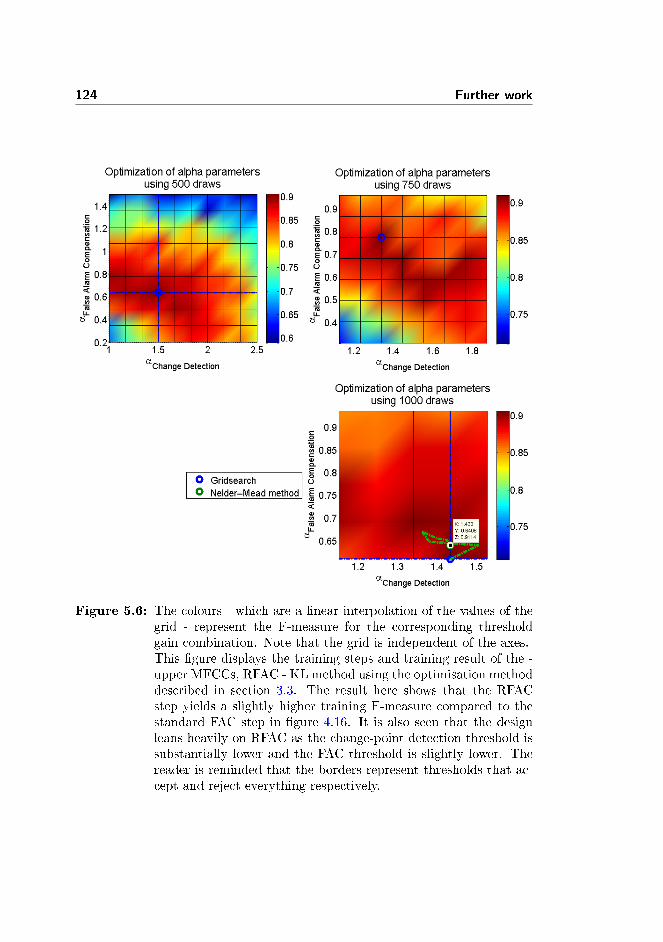
124 Further work
Figure 5.6: The colours - which are a linear interpolation of the values of thegrid - represent the F-measure for the corresponding thresholdgain combination. Note that the grid is independent of the axes.This �gure displays the training steps and training result of the -upper MFCCs, RFAC - KL method using the optimisation methoddescribed in section 3.3. The result here shows that the RFACstep yields a slightly higher training F-measure compared to thestandard FAC step in �gure 4.16. It is also seen that the designleans heavily on RFAC as the change-point detection threshold issubstantially lower and the FAC threshold is slightly lower. Thereader is reminded that the borders represent thresholds that ac-cept and reject everything respectively.
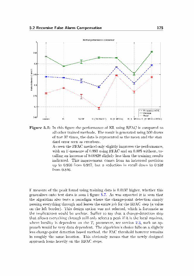
5.2 Recursive False Alarm Compensation 125
Figure 5.7: In this �gure the performance of KL using RFAC is compared toall other trained methods. The result is generated using 500 drawsof test 37 times, the data is represented as the mean and the stan-dard error seen as errorbars.As seen the RFAC method only slightly improves the performance,with an F-measure of 0.893 using RFAC and an 0.885 without, to-talling an increase of 0.00828 slightly less than the training resultsindicated. This improvement comes from an increased precisionup to 0.956 from 0.927, but a reduction in recall down to 0.838from 0.846.
F-measure of the peak found using training data is 0.0137 higher, whether thisgeneralises onto test data is seen i �gure 5.7. As was expected it is seen thatthe algorithm also tests a paradigm where the change-point detection simplypassing everything through and leaves the entire job for the RFAC step (a valueon the left border). This design option was not selected, which is fortunate asthe implications would be unclear. Su�ce to say that a change-detection stepthat allows everything through still only selects a peak if it is the local maxima,where locality is dependent on the Ti parameter, see section 2.3, such an ap-proach would be very data dependent. The algorithm's choice falls on a slightlyless change-point detection based method, the FAC threshold however remainsin roughly the same location. This obviously means that the newly designedapproach leans heavily on the RFAC steps.
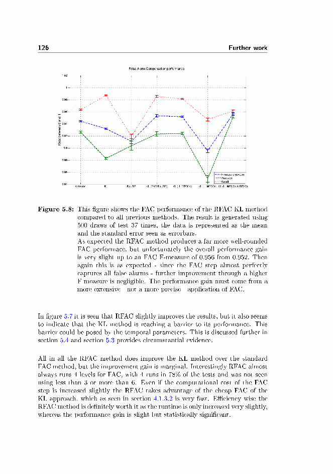
126 Further work
Figure 5.8: This �gure shows the FAC performance of the RFAC KL methodcompared to all previous methods. The result is generated using500 draws of test 37 times, the data is represented as the meanand the standard error seen as errorbars.As expected the RFAC method produces a far more well-roundedFAC performace, but unfortunately the overall performance gainis very slight up to an FAC F-measure of 0.956 from 0.952. Thenagain this is as expected - since the FAC step almost perfectlycaptures all false alarms - further improvement through a higherF-measure is negligible. The performance gain must come from amore extensive - not a more precise - application of FAC.
In �gure 5.7 it is seen that RFAC slightly improves the results, but it also seemsto indicate that the KL method is reaching a barrier to its performance. Thisbarrier could be posed by the temporal parameters. This is discussed further insection 5.4 and section 5.3 provides circumstantial evidence.
All in all the RFAC method does improve the KL method over the standardFAC method, but the improvement gain is marginal. Interestingly RFAC almostalways runs 4 levels for FAC, with 4 runs in 78% of the tests and was not seenusing less than 3 or more than 6. Even if the computational cost of the FACstep is increased slightly the RFAC takes advantage of the cheap FAC of theKL approach, which as seen in section 4.1.3.2 is very fast. E�ciency wise theRFAC method is de�nitely worth it as the runtime is only increased very slightly,whereas the performance gain is slight but statistically signi�cant.

5.3 Mimicking news pod-cast data 127
Figure 5.9: This �gure shows the percentage of false alarms for the RFACmethod. Unexpectedly the percentage of false alarms only wentup very slightly, by about 1 percentage point, compared to theupper MFCC KL standard FAC method.
This section did not make it into the greater body of work since the e�ect of aset number of FAC runs, rather than a fully recursive one is left unexplored dueto a lack of computational resources.
5.3 Mimicking news pod-cast data
Upon a closer inspection of the results using KL with RFAC and upper MFCCs,an interesting discovery was made. It was found that the method did surprisinglywell, except in the case of very short speaker turns in rapid succession, herereferring to speaker turns at a length of about 2 seconds. In the news pod-castscenario this type of conversation is very rare and as seen in Jørgensen et al.[55] speaker segments below 5 seconds in general are uncommon.
As an experiment and to mediate better comparison with other work, the KLmodel already trained is simply fed data with speaker turns lengths alwaysabove 5 seconds. The result of this trial is seen in �gure 5.10 and as seenthe performance without short speaker turns is far greater than with. TheF-measure increases to 0.940 with a precision of 94.3%, and a recall of 93.7%.

128 Further work
Figure 5.10: This �gure shows that the performance of the KL method - us-ing RFAC and upper MFCCs - is far greater if the speech datadoes not contain short speaker turns (<5s). With the F-measureincreasing to 0.940 having a precision of 94.3%, and a recall of93.7%.

5.4 Promising avenues 129
This result is very promising as the optimisation method designed in this thesiscould be exported onto commercial software. The commercial software couldthen train the algorithm to its particular speech data and performance couldfar exceed the general case performance.
This section is not admitted into the greater body of work, as mimicking thedistribution of speaker turn lengths found in news pod-casts, goes far beyondthe fairly arbitrary limit of min. 5 seconds of speech.
5.4 Promising avenues
This section will quickly enumerate promising unexplored avenues in bullet-pointform.
• In section 2.2.3 several methods for reducing the e�ect of noise were inves-tigated. Beyond this, code was developed for generating data immersedin varying SNR of several noise types, including babble noise, white noiseand potentially noise caused by phone-line compression. As was mentionedMFCCs have been found to handle noise poorly and this might reveal in-teresting strengths and weaknesses in the various approaches. For instancesection 3.2.2.2 mentions research where KL was found to be weak in a noisyenvironment.
• During the RuLSIF implementation, see section 3.2.3.3, the smoothingparameter αR was left at its default setting. An optimisation of this pa-rameter might increase the performance of RuLSIF, however as RuLSIF'sweakness lies in its e�ciency this avenue was barely explored.
• More promisingly it was found that RuLSIF's e�ciency could be optimisedsigni�cantly in section 3.2.3.3. This would require tampering with itscross-validation step of the kernel width and its regularization parameter.This cross-validation is performed in every single density-ratio estimationindividually, which is probably excessive, as test revealed that the rangeof values selected was quite tight. If this cross-validation step could beskipped entirely its e�ciency could be improved by up to a factor of 4.
• The change-point detection algorithm, the FAC algorithm and the MFCCcalculation have a number of temporal parameters, in this thesis all thesewere borrowed from previous work. The majority of these were optimisedby Jørgensen et al. [55] for a vector quantization based approach. Asthe selected method in this thesis is not based on vector quantization, atuning of these parameters might increase performance.

130 Further work
• In section 2.4 alternatives to the FAC based SCD was mentioned. Insection 4.1.3.1 results indicated that a combination of the ensemble basedapproach with with the FAC based approach might be promising.
• In section 4.1.3.1 it was hypothesized that RuLSIF might bene�t signif-icantly e�ciency wise, if the optimisation algorithm from section 3.3 in-cluded e�ciency in its optimisation goal.
• Finally in section 4.4 it is concluded that a full backwards feature selectionof KL using the optimisation technique developed in section 3.3 wouldlikely result in a marked improvement. This would however be a verycostly process computationally.

Chapter 6
Final conclusions
This thesis has investigated, implemented, contrasted and combined a widerange of methods for speaker change detection using segmentation, and sub-sequently selected a method on which novel improvements have been imple-mented. These improvements revolve around a custom parameter optimisationtechnique for automatic model selection, a fully recursive speaker change detec-tion paradigm and a model of the human speech production system. In additionthe �eld of speaker clustering has been propped to fully resolve the problem ofspeaker diarisation, the question of "who spoke when?".
The investigated speaker change detection methods were drawn from the �eldsof vector quantization, Gaussian processes and relative density-ratio estimation,a novel approach from general change-detection theory not previously appliedto speaker change detection. These methods mainly included an optimised K-means algorithm, the Kullback-Leibler distance, KL, and Relative unconstrainedLeast-Squares Importance Fitting, RuLSIF, respectively.
As the available speech corpora, ELSDSR & TIMIT, are designed for speechrecognition, a novel method for generating speaker change detection data fromELSDSR was designed. This method solves the issues of �le splicing, of non-uniform speech sample lengths and of the limited combinatorial nature of thecorpora using a custom algorithm based on data bootstrapping. This methodis designed to test the methods to their limit, capable of generating a broad

132 Final conclusions
range of change-point sequence types; anything from rapid-�re arguments tolong monologues.
A broad search into the feature extraction techniques commonly applied tospeaker change detection is conducted. Through a literary study a list of re-quirements for the feature set is established. It is found that short-term spectralfeatures meet all requirements, yield decent performance and are easy to com-pute. Within short-term spectral features, particularly the Mel-Frequency Cep-stral Coe�cients are selected as they �eld a sound theoretical basis. The conceptis to deconvolve the person speci�c excitation signal of the voicebox from theliteral-semantic speci�c �ltering of the vocal tract. The literary study found theamount of the Mel-Frequency Cepstral Coe�cients, the use of derivatives andtheir placement in the cepstrum to be very diverse. This thesis employs severalstages of feature selection to deal with this issue.
K-means, KL and RuLSIF, among others, were compared to various degrees ofprecision before these main contenders remained. Along with these a hybridcombination of KL and RuLSIF was designed to incorporate both the e�ciencyof KL and the thoroughness of RuLSIF. These 4 methods were fed through thecustom optimisation algorithm using training data and tested on test data.
Out of the resulting optimised methods K-means �elded the highest F-measureof 0.84, with 93.4% of hypothesised change-point being true and �nding 76.3%of all possible change-points. Whereas RuLSIF and the RuLSIF/KL hybridfailed to utilise the optimisation algorithm fully, due to e�ciency issues. The KLmethod however came in as a close second, �elding an F-measure only 0.05 lowerthan K-means using a more well-rounded approach. KL only had a precisionof 88.9%, but succeeded in locating 78.8% of the total change-points, meaningthat KL in spite of being the simplest method displayed the greatest potentialfor improvement. Beyond this the KL approach has a closed form solutionand therefore clocks in at 2.5 times faster than K-means despite the e�ciencyimprovements reducing the runtime of K-means 15-fold, with KL running at 5times real-time. Due to e�ciency, the possible hidden potential and the closeperformance scores, KL was chosen.
KL subsequently underwent a series of improvements involving a backwardsfeature selection based on the model of the human speech production systemand a fully recursive false alarm compensation paradigm. This process resultedin an F-measure of 0.893. This improvement comes from an increased precisionup to 95.6%, with the method �nding 83.8% of change-points, at almost nodecrease in e�ciency.
Upon close inspection almost all missed change-points were found in rapid-�re speech, with speaker-turns of about 2 seconds, in which case the algorithm

133
often combined multiple speaker changes into a single speaker change. Using thesame parameter set the F-measure increases to 0.940 using data with speakerturns always above 5 seconds, here with a precision of 94.3%, while locating93.7% of all change-points. This result is very promising as the optimisationmethod designed in this thesis could be exported onto commercial software. Thecommercial software could then train the algorithm to its particular speech dataautomatically and performance could far exceed the general case performance.

134 Final conclusions

Appendix A
MATLAB Code
For the sake of transparency, all essential functions for reproducing results areincluded here. Peripheral code such as toolboxes, plotting functions, �le man-agement, scripts, etc. are excluded.
A.1 Main Scripts
A.1.1 Main: Speaker Change Detection
1 %% enable wrapper func t i on2 i f e x i s t ( 'wrapper_ON ' )3 wrapper_OFF = 0 ;4 enable_data_plots = 0 ;5 e l s e6 c l c ; c l e a r a l l ; c l o s e a l l ;7 wrapper_OFF = 1 ;8 change_points = 50 ;9 i f change_points > 10010 enable_data_plots = 0 ;11 e l s e

136 MATLAB Code
12 enable_data_plots = 1 ;13 end14 RandStream . setDefau l tStream . . .15 (RandStream( ' mt19937ar ' , ' seed ' , sum(100∗ c l o ck ) ) ) ;16 end17
18 %% Change Point Detect ion parameters19 % Parameters ( va lue s taken from Lasse s e c t i o n 4 . 4 . 4 , law
= 3s , Ti = 2s , Tmax = 8s , and l s = 0 .1 s . )20 l_aw = 3 ;21 l_s = 0 . 1 ;22 Tmax = 8 ;23 Ti = 2 ; % the width o f a changepoint , another chanpoint
must be out s id e t h i s width . I t i s o f cause centered onthe changepoint
24 bu f f e r = Ti /2 ; %dont use data with in x seconds o fsurrounding change po in t s f o r f a l s e alarm compensation
25 i f wrapper_OFF == 126 alpha_cd .VQD = 1 . 1 1 3 ;%56 : 1 . 0 9 6 ; %25: 1 . 1 1 3 ;27 alpha_cd .KL = 1 . 7 0 3 ;%lowermfcc 1.6656%
uppermfcc 1.6621;% p la in 1.703;% r u l s i f 2 . 0 003 ;28 alpha_cd .DSD = 1 . 3 ;29 alpha_cd . RuLSIF = 1 . 4 8 3 ;30
31 alpha_fac .VQD = 0 . 9085 ;%56 : 0 . 9 155 ; %25:0 .9085
32 alpha_fac .KL = 0 . 4324 ;%lowermfcc 0.6892%uppermfcc 0.6643;% p la in 0.4324;% r u l s i f 2 . 0 500 ;
33 alpha_fac .DSD = 0 . 4 ;34 alpha_fac . RuLSIF = 0 . 9 5 ;35 end36
37 %% samplerate38 f s = 16000 ;39
40 %% Change po int de t e c t i on methods41 i f wrapper_OFF == 142 method_list = { 'k−means ' , 'KL ' , 'DSD ' , 'RuLSIF ' } ;43 end44
45 %% False alarm compensation methods46 % CP method order : ' k−means ' 'KL' 'DSD' 'RuLSIF '47
48 fac_methods = { 'k−means ' , 'KL ' , 'DSD ' , 'RuLSIF ' } ;

A.1 Main Scripts 137
49
50 i f wrapper_OFF == 051 fac_methods{ strcmp (method_list , { 'k−means ' , 'KL ' , 'DSD ' ,
'RuLSIF ' }) } = fac_method ;52 end53 %% Read data54 type = ' t r a i n ' ;55 shor te s t_length = 1 ;56 combine_method = 'LHKs ' ;57
58 [ data time_info ] = combinee l sdsr ( change_points ,wrapper_OFF , type , shortes t_length , f s , combine_method ) ;
59
60 %% Read changepoints61 Read_actual_changepoints_section62
63 %% Remove non−speech par t s64 % Remove_nonspeech_parts_section %in a c t i v e65
66 %% add no i s e67 % input_no i s e_f i l e = ' babble ' ;68 % SNRdB = 100 ;69 % add_noise70
71 %% Feature ex t r a c t i on72 Feature_extract ion_sect ion73
74 %% Divide ceps in to segments75 ceps_segmentat ion_sect ion76
77 %% VQD using K−means78 i f sum( strcmp (method_list , ' k−means ' ) )~=079
80 di sp ( 'WARNING: k_means hardcoded to only use f i r s t 12MFCCs, a l s o in FAC! ' )
81 ceps_temp = ceps ;82 ceps = ceps ( : , 1 : 1 2 ) ;83 g l oba l K84 K = 25 ;85
86 Kmeans_VQD_section87
88 ceps = ceps_temp ;89 end

138 MATLAB Code
90
91 %% KL & DSD us ing s i n g l e mu l t i va r i an t gauss ian model92 KL_DSD_section93
94 %% RuLSIF95 i f sum( strcmp (method_list , 'RuLSIF ' ) )~=096 alpha = . 1 ; % Smoothing parameter97 s igma_l i s t = 0 . 2 : 0 . 4 : 2 ; % Kernel Width98 lambda_list = −6:1:−2; % Regura l i z a t i on parameter99 n = seg_length ;100 s tep = seg_shi f t_length ;101 k_folds = 5 ;102 RuLSIF_section103 end104
105 %% Calcu la te timestamps106 x_axis = ( seg_start_samples ( 1 : end−seg_overlap )+(
seg_length−1) ) . / mfcc_opts . mfccprsec ; %a f t e r thesegment s i n c e the changepoint i s measured inbetween 2segments
107
108 %% mark change po in t s ( Ca l cu la t e VQD_n, avr & th_cd , n (Lasse ' s r epo r t page 62) )
109 Mark_change_points_section110
111 %% False alarm compensation (VQD)112 any_FAC_updates=1;113 any_FAC_updates_count = 1 ;114 whi le (any_FAC_updates~=0) %Keeps running u n t i l l no
changepo ints are marked as f a l s e115 FAC_section116 any_FAC_updates_count = any_FAC_updates_count + 1 ;117 end118
119 %% f−measure120 F_measure_section121
122 %% FAC performance123 FAC_performance_section124
125 %% Plo t t i ng126 i f wrapper_OFF == 1127 main_fig = f i g u r e ;128

A.1 Main Scripts 139
129 i f enable_data_plots == 1 ;130 % Compute and p lo t Spectrogram of data131 Spectrogram_section132
133 % plo t MFCCs134 Feature_plott ing_sect ion135 end136
137 % plo t Metr ics and CPs138 Metr ic_plott ing_sect ion139 end140
141 %% ROC142 i f wrapper_OFF == 1143 ROC_section144 end
A.1.2 Main: Speaker Clustering
1 c l c ; c l e a r a l l ; c l o s e a l l ;2 f s = 16000 ;3 Tmax = 8 ;4 runs = 5 ;5
6 f i g u r e7 f o r n_out = 1 : runs8 %% Read data9 N_segment = 500 ;10 N_people = 5 ; %t r a i n i n g max 23 %obs , s imply wanting
a l l the data i s not p o s s i b l e ( s i n c e i a l s o usesub s e c t i on s o f data as i nd i v i dua l data ) %obs ,s i n c e the data i s drawn randomly the datase t mightnot conta in the f u l l amount o f speaker s
11 type = ' t r a i n ' ;12 shor te s t_length = 3 ;13 fs_out = 16000 ;14 [ input chosen_names ] = e l s d s r_c l u s t e r i n g (N_segment ,
N_people , type , shortest_length , fs_out ) ;15
16 %% Feature ex t r a c t i on17 f o r n = 1 : s i z e ( input , 1 )18 data = input {n , 1 } ;19 Feature_extract ion_sect ion

140 MATLAB Code
20 Tmax_influence = Tmax∗mfcc_opts . mfccprsec ;21 input {n ,3} = ceps ;22 end23
24 input_orig = input ( randperm ( s i z e ( input , 1 ) ) , : ) ; %s h u f f l e input
25
26 %% c l u s t e r i n g metr ic27 method_list = { 'KL ' , 'DSD ' , ' k−means ' , 'RuLSIF ' , 'BIC ' , '
ICR ' } ;28
29 f o r n_method = 1 : numel ( method_list )30 method = method_list {n_method } ;31 input = input_orig ;32
33 f i g u r e (n_method)34 i ndexes = 1 :N_segment ;35 n = 1 ;36 whi le (1 )37
38 %% compute d i s t matrix39 dist_matrix = 1e6 .∗ ones ( s i z e ( input , 1 ) ) ; %
cons t ruc t d i s t ance matrix40 % wbar = waitbar ( 0 , [ ' C lu s t e r i ng
us ing ' method ] ) ;41 lower_triangle_and_diag = 1 ;42 f o r row = 1 : s i z e ( input , 1 )43 f o r c o l = (1+lower_triangle_and_diag ) :
s i z e ( input , 1 )44
45 A = input {row , 3 } ;46 B = input { co l , 3 } ;47
48 i f s i z e (A, 1 )>Tmax_influence | | s i z e (B, 1 )>Tmax_influence
49 i f s i z e (A, 1 )>Tmax_influence50 tmp = randperm ( s i z e (A, 1 ) ) ;51 A = A(tmp ( 1 : Tmax_influence )
, : ) ;52 end53 i f s i z e (B, 1 )>Tmax_influence54 tmp = randperm ( s i z e (B, 1 ) ) ;55 B = B(tmp ( 1 : Tmax_influence )
, : ) ;

A.1 Main Scripts 141
56 end57
58 dist_matrix ( row , c o l ) =compare_segments (A,B, method ) ;
59 e l s e60 dist_matrix ( row , c o l ) =
compare_segments (A,B, method ) ;61 end62
63 end64 lower_triangle_and_diag =
lower_triangle_and_diag+1;65 end66
67 %% f ind more common segments68 [ mins (n) , I ] = min ( dist_matrix ( : ) ) ;69 [ row , c o l ] = ind2sub ( s i z e ( dist_matrix ) , I ) ;70
71 %% combine l i k e l y cond idate s72 number_added (n) = sum( input { co l , 2 } ) ;73 Z(n , : ) = [ indexes ( row ) indexes ( c o l ) mins (n) ] ;74
75 input {row ,1} = [ input {row , 1 } ; input { co l , 1 } ] ;76 input {row ,2} = input {row ,2} + input { co l , 2} ;77 input {row ,3} = [ input {row , 3 } ; input { co l , 3 } ] ;78 i ndexes ( row ) = N_segment+n ;79
80 input ( co l , : ) = [ ] ;81 i ndexes ( c o l ) = [ ] ;82
83 %% pur i ty84 pur i ty = ze ro s ( s i z e ( input , 1 ) , 1 ) ;85 f o r n2 = 1 : s i z e ( input , 1 )86 pur i ty ( n2 ) = max( input {n2 , 2 } ) /sum( input {
n2 , 2 } ) ;87 end88 purity_avg ( s i z e ( input , 1 ) , n_out , n_method) =
mean( pur i ty ) ;89 c l e a r pur i ty90
91 %% c l u s t e r s i z e s92 s i z e s = ze ro s ( s i z e ( input , 1 ) ,1 ) ;93 f o r n2 = 1 : s i z e ( input , 1 )94 s i z e s ( n2 ) = sum( input {n2 , 2 } ) ;

142 MATLAB Code
95 end96 min_clust_size ( s i z e ( input , 1 ) , n_out , n_method)
= min ( s i z e s ) ;97 max_clust_size ( s i z e ( input , 1 ) , n_out , n_method)
= max( s i z e s ) ;98 avg_clust_size ( s i z e ( input , 1 ) , n_out , n_method)
= mean( s i z e s ) ;99
100 i f sum( s i z e s > 1) == N_people101 save_s i ze s {n_method} = s i z e s ;102 va l i d_c lu s t (n) = 1 ;103 e l s e104 va l i d_c lu s t (n) = 0 ;105 end106
107 %% break cond i t i on108 i f ( s i z e ( input , 1 )==1)109 break ;110 end111
112 %% plo t113 dist_matrix ( dist_matrix==1e6 )=max( dist_matrix
( dist_matrix~=1e6 ) ) ;114 imagesc ( dist_matrix , [ min ( dist_matrix ( : ) ) max(
dist_matrix ( : ) ) ] )115 co l o rba r116 drawnow ;117
118 %loop counter119 n=n+1;120 end121 c l o s e (n_method)122 %%123 i f runs == 1124
125 i f (min (Z ( : , 3 ) ) < 0)126 Z ( : , 3 ) = Z ( : , 3 ) − min(Z ( : , 3 ) ) + 1 ;127 neg = 1 ;128 e l s e129 neg = 0 ;130 end131
132 i f sum( va l i d_c lu s t ) > 0133 index = max( f i nd ( va l i d_c lu s t ) ) ;

A.1 Main Scripts 143
134 th r e sho ld = Z( index+1 ,3) ∗1 . 0 01 ;135 e l s e136 di sp ( ' Using d e f au l t th r e sho ld ' )137 th r e sho ld= . 7∗ (max(Z ( : , 3 ) ) ) ;138 end139
140 i f strcmp ( method_list {n_method} , 'ICR ' )141 Z ( : , 3 ) = log10 (Z ( : , 3 ) ) ;142 th r e sho ld = log10 ( th r e sho ld ) ;143 l ogy = 1 ;144 e l s e145 l ogy = 0 ;146 end147
148 f ont = 13 ;149 f i g u r e150 [H,T, perm ] = dendrogram (Z , 0 , ' c o l o r t h r e s h o l d ' ,
th r e sho ld ) ;%' de fau l t ' ) ;151 s e t (H, ' LineWidth ' , 2 )152 hold a l l153 h l e g l i n e s = [ ] ;154 f o r n2 = 1 : N_people155 dots = [ ] ;156 f o r n = 1 :N_segment157 index = perm(n) ;158 i f input_orig { index , 2 } ( n2 ) == 1159 dots = [ dots n ] ;160 end161 end162 tmp = p lo t ( dots , z e r o s (1 , l ength ( dots ) )
+0.001∗max(Z ( : , 3 ) ) , ' . ' , ' markers i ze ', 20) ;
163 l egends {n2} = [ ' Speaker #' num2str ( n2 ) ] ;164 h l e g l i n e s = [ h l e g l i n e s tmp ] ;165 end166 p lo t ( 1 : N_segment , th r e sho ld .∗ ones (1 ,N_segment )
, ' k−. ' , ' l i n ew id th ' , 3 )167
168 y l ab l = method_list {n_method } ;169 i f neg == 1170 y l ab l = [ y l ab l '+ (−min( ' y l ab l ' ) ) + 1 '
] ;171 end172 i f l ogy == 1

144 MATLAB Code
173 y l ab l = [ ' log10 ( ' y l ab l ' ) ' ] ;174 end175
176 y l ab e l ( [ ' C lus te r d i s s im i l a r i t y [ ' y l ab l ' ] ' ] ,' f o n t s i z e ' , f ont )
177 x l ab e l ( ' Fu l l Speaker segment index ( orderi r r e l e v a n t ) ' , ' f o n t s i z e ' , f ont )
178 t i t l e ( [ 'Dendrogram of f u l l speaker segmentsus ing Agglomerative H i e r a r c h i c a lC lu s t e r i ng with ' method_list {n_method} 'c l u s t e r d i s s im i l a r i t y measure ' ] , ' f o n t s i z e ', f ont )
179 l egend ( h l e g l i n e s , l egends , ' Locat ion ' , 'northwest ' ) ;
180 s e t ( gca , ' f o n t s i z e ' , 13)181 end182 end183 end
A.2 Parameter Optimisation
A.2.1 Main: Parameter Optimisation
1 c l c ; c l e a r a l l ; c l o s e a l l ;2
3 RandStream . setDefau l tStream . . .4 (RandStream( ' mt19937ar ' , ' seed ' , sum(100∗ c l o ck ) ) ) ;5
6 r e s o l u t i o n s = [10 5 ] ;7 data_amounts = [500 10 00 ] ;8 remove_bound_percentage = 50 ;9 cd_method = 'KL ' ;10 fac_method = 'KL ' ;11 re runs = 3 ;12
13 no_fac = 0 ;14 maxiter = 30 ;15
16 cd_bound = [ 1 . 0 2 . 5 ] ;17 fac_bound = [ 0 . 2 1 . 5 ] ;18

A.2 Parameter Optimisation 145
19 r e s o l u t i o n s = round ( l i n s p a c e ( r e s o l u t i o n s (1 ) , r e s o l u t i o n s(2 ) , r e runs ) )
20 data_amounts = round ( l i n s p a c e ( data_amounts (1 ) ,data_amounts (2 ) , r e runs ) )
21
22 cd_center = mean( cd_bound) ;23 fac_center = mean( fac_bound ) ;24 cd_range = range ( cd_bound) ;25 fac_range = range ( fac_bound ) ;26
27 ID = f l o o r ( rand∗1 e6 )+1;28 di sp ( ID)29
30 f i g u r e31 f o r rerun = 1 : re runs32
33 r e s o l u t i o n = r e s o l u t i o n s ( rerun ) ;34 data_amount = data_amounts ( rerun ) ;35
36 cd_range = range ( cd_bound) ∗( remove_bound_percentage/100) ^( rerun−1) ;
37 fac_range = range ( fac_bound ) ∗(remove_bound_percentage /100) ^( rerun−1) ;
38
39 cd_bound_current (1 ) = cd_center−cd_range /2 ;40 cd_bound_current (2 ) = cd_center+cd_range /2 ;41
42 i f cd_bound_current (1 )<cd_bound (1)43 cd_bound_current = cd_bound_current+(cd_bound (1)−
cd_bound_current (1 ) ) ;44 e l s e i f cd_bound_current (2 )>cd_bound (2)45 cd_bound_current = cd_bound_current−(
cd_bound_current (2 )−cd_bound (2) ) ;46 end47
48 fac_bound_current (1 ) = fac_center−fac_range /2 ;49 fac_bound_current (2 ) = fac_center+fac_range /2 ;50
51 i f fac_bound_current (1 )<fac_bound (1)52 fac_bound_current = fac_bound_current+(fac_bound
(1)−fac_bound_current (1 ) ) ;53 e l s e i f fac_bound_current (2 )>fac_bound (2)54 fac_bound_current = fac_bound_current−(
fac_bound_current (2 )−fac_bound (2) ) ;

146 MATLAB Code
55 end56
57 cd = l i n s p a c e ( cd_bound_current (1 ) , cd_bound_current(2 ) , r e s o l u t i o n )
58 f a c = l i n s p a c e ( fac_bound_current (1 ) , fac_bound_current(2 ) , r e s o l u t i o n )
59
60 i f no_fac == 161 f a c = fac (1 ) ;62 end63
64 gdvalues = {cd f a c } ;65
66 i f rerun == reruns && maxiter~=067 fminON = 1 ;68 e l s e69 fminON = 0 ;70 end71
72 addarg = {cd_method , fac_method , data_amount } ;73 [ x co s t f v a l e x i t f l a g output x_al l f v a l_a l l ] =
simpgdsearch ( ' obj fun ' , gdvalues , addarg , ' temp . txt ' ,fminON , maxiter ) ;
74
75 cd_center = x (1) ;76 fac_center = x (2) ;77 %% save in te rmed ia t e c a l c s78 mat_name = [ ' cd method ' cd_method ' f a c method '
fac_method ' run ' num2str ( rerun ) ' out o f 'num2str ( re runs ) ' ID ' num2str ( ID) ] ;
79 save (mat_name)80
81 %% Plot r e s u l t s82 i f e x i s t ( ' no_fac ' ) == 1 && no_fac == 183 p lo t ( cd ,1− cost , '−o ' , ' l i n ew id th ' , 2 )84 hold a l l85 xlim ( [ cd_bound ] )86 ylim ( [ 0 1 ] )87 i f rerun == reruns88 p lo t ( x_al l ( : , 1 ) ,1− f va l_a l l , '−o ' , ' l i n ew id th '
, 2 )89 p lo t ( x ( : , 1 ) ,1− f va l , '−x ' , ' l i n ew id th ' ,10)90 end91 e l s e

A.2 Parameter Optimisation 147
92 optim_parameter_plott ing_section93 end94 end
A.2.2 Objective Function
1 f unc t i on f = obj fun ( parameters , addarg )2
3 f = 1−Main_wrapper ( addarg {1} , parameters (1 ) , parameters (2 ) ,addarg {3} , addarg {2}) ;
A.2.3 Parameter Optimisation
1 f unc t i on [ x co s t minval e x i t f l a g output x_al l f v a l_a l l ] =simpgdsearch ( objfun , gdvalues , addarg , f i l e o u t , fminON ,
maxiter )2 %% number o f dimensions3 nd = s i z e ( gdvalues , 2 ) ;4
5 %% crea t e parameter s tep6 f o r k = 1 : nd7 paramstep (k , : ) = gdvalues ;8 end9
10 %% model : a l l the combination o f the eva luated parameters11 s t r = [ ] ;12 f o r k = 1 : nd13 s t r = [ s t r ' gdvalues { ' num2str ( k ) ' } , ' ] ;14 end15 s t r ( l ength ( s t r ) ) = [ ] ;16 eva l ( [ ' model = setprod ( ' s t r ' ) ; ' ] ) ;17
18 %% gr id search19 time = 0 ;20 co s t = ze ro s (1 , s i z e (model , 1 ) ) ;21 wbar = waitbar (0 , ' P lease wait . . ' ) ;22 f o r l = 1 : s i z e (model , 1 )23 in terna l_t ime = t i c ;24
25 i f ( l ~=1)26 average_runtime = time /( l −1) ;27 runs_le f t = s i z e (model , 1 )−( l −1) ;28 t ime_le f t = runs_le f t ∗average_runtime ;

148 MATLAB Code
29 t ime_le f t_st r ing = [ ' Time l e f t : ' secs2hms (t ime_le f t ) ] ;
30 waitbar ( l / s i z e (model , 1 ) ,wbar , s p r i n t f ( '%s ' ,t ime_le f t_st r ing ) )
31 di sp ( t ime_le f t_st r ing )32 end33
34 co s t ( l ) = f e v a l ( objfun , model ( l , : ) , addarg ) ;35
36 time = time + toc ( interna l_t ime ) ;37 end38 de l e t e (wbar )39
40 %% best f i t model %%41 [ minval ind ] = min ( co s t ) ;42 x_grid = model ( ind , : ) ;43 x = x_grid ;44
45 e x i t f l a g = [ ] ;46 output = [ ] ;47 i f fminON ==148 %% Simplex method %%49 opt ions = opt imset ( ' Display ' , ' i t e r ' , 'TolX ' , 0 . 0 1 , '
TolFun ' ,1 e10 , ' MaxIter ' , maxiter , 'OutputFcn ' ,@outfun ) ; %
50 [ x , f va l , e x i t f l a g , output , x_all , f v a l_a l l ] = fminsearch( objfun , x , opt ions , addarg ) ;
51
52 x_al l = [ x_grid ; x_al l ] ;53 f v a l_a l l = [ minval ; f v a l_a l l ] ;54
55 minval = f v a l ;56
57 %% save data %%58 i f narg in == 459 f oo = [ model , cost ' ] ;60 f oo = [ foo ; x , f v a l ] ;61 save ( f i l e o u t , ' f oo ' , '−a s c i i ' ) ;62 end63 e l s e64 x_al l = x ;65 f v a l_a l l = minval ;66 end

A.3 SCD Methods 149
A.3 SCD Methods
A.3.1 Main: Gaussian approach section
1 i f sum( strcmp (method_list , 'KL ' ) )~=0 | | sum( strcmp (method_list , 'DSD ' ) )~=0
2 % ML es t o f s i n g l e gauss ian on each segment3 i f wrapper_OFF == 14 wbar = waitbar (0 , 'ML est imate o f sigma and mu ' ) ;5 end6 ML_est_timer = t i c ;7 sigma = ze ro s ( s i z e ( ceps , 2 ) , s i z e ( ceps , 2 ) , l ength (
seg_start_samples ) ) ;8 mu = ze ro s ( s i z e ( ceps , 2 ) , l ength ( seg_start_samples ) ) ;9
10 f o r n_seg = 1 : l ength ( seg_start_samples )11 i f wrapper_OFF == 112 waitbar ( n_seg/ l ength ( seg_start_samples ) ) ;13 end14
15 ceps_seg = ceps_seg_func ( n_seg , seg_start_samples ,ceps , seg_length ) ;
16 sigma ( : , : , n_seg ) = cov ( ceps_seg ) ;17 mu( : , n_seg ) = mean( ceps_seg ) ;18 end19 i f wrapper_OFF == 120 de l e t e (wbar )21 end22 time .ML_est = toc (ML_est_timer ) ;23 end24
25 i f sum( strcmp (method_list , 'KL ' ) )~=026 % Kullback Le i b l e r d ive rgence27 i f wrapper_OFF == 128 wbar = waitbar (0 , 'KL ' ) ;29 end30 KL_timer = t i c ;31 KLs = ze ro s ( l ength ( seg_start_samples )−seg_overlap , 1 ) ;32 f o r n_seg = 1 : l ength (KLs)33 i f wrapper_OFF == 134 waitbar ( n_seg/ l ength (KLs) ) ;35 end36

150 MATLAB Code
37 KLs( n_seg ) = KL( sigma ( : , : , n_seg ) , sigma ( : , : , n_seg+seg_overlap ) ,mu( : , n_seg ) ,mu( : , n_seg+seg_overlap ) ) ;
38 end39 time .KL = toc (KL_timer ) ;40 i f wrapper_OFF == 141 de l e t e (wbar )42 end43 end44
45 i f sum( strcmp (method_list , 'DSD ' ) )~=046 % Divergence Shape Distance47 i f wrapper_OFF == 148 wbar = waitbar (0 , 'DSD ' ) ;49 end50 DSD_timer = t i c ;51 DSDs = ze ro s ( l ength ( seg_start_samples )−seg_overlap , 1 )
;52 f o r n_seg = 1 : l ength (DSDs)53 i f wrapper_OFF == 154 waitbar ( n_seg/ l ength (DSDs) ) ;55 end56
57 DSDs( n_seg ) = DSD( sigma ( : , : , n_seg ) , sigma ( : , : ,n_seg+seg_overlap ) ) ;
58 end59 time .DSD = toc (DSD_timer) ;60 i f wrapper_OFF == 161 de l e t e (wbar )62 end63 end
A.3.2 Kullback Leibler distance
1 f unc t i on out = KL(sigma_A , sigma_B ,mu_A,mu_B)2 %KL: Kullback−Le i b l e r Distance3
4 out = 1/2∗ t r a c e ( ( sigma_A − sigma_B) ∗( inv ( sigma_B) − inv (sigma_A) ) + . . .
5 1/2∗ t r a c e ( ( inv ( sigma_A) + inv ( sigma_B) ) ∗(mu_A −mu_B) ∗(mu_A − mu_B) ' ) ) ;
6
7 end

A.3 SCD Methods 151
A.3.3 Divergence Shape Distance
1 f unc t i on out = DSD(sigma_A , sigma_B)2
3 out = 1/2∗ t r a c e ( ( sigma_A − sigma_B) ∗( inv ( sigma_B) − inv (sigma_A) ) ) ;
4
5 end
A.3.4 Main: Vector Quantization section
1
2 %% Calcu la te codebooks3 warning ( ' o f f ' , ' a l l ' ) ;4 i f wrapper_OFF == 15 wbar = waitbar (0 , 'K−means ' ) ;6 end7 kmeans_timer = t i c ;8 kmeans_opts = s t a t s e t ( ' MaxIter ' ,10000) ;9
10 c en t r o i d s = ze ro s (K, s i z e ( ceps , 2 ) , l ength ( seg_start_samples) ) ;
11 f o r n_seg = 1 : l ength ( seg_start_samples )12 i f wrapper_OFF == 113 waitbar ( n_seg/ l ength ( seg_start_samples ) ) ;14 end15
16 ceps_seg = ceps_seg_func ( n_seg , seg_start_samples , ceps, seg_length ) ;
17
18 % Optimized by pas s ing on old cent ro id s , ~2.5 t imesf a s t e r . (OBS! This a l s o smoothes the r e su l t , thusdegrading i t . )
19 i f n_seg ~= 120 % [ IDX, c en t r o i d s ( : , : , n_seg ) ] = kmeans ( ceps_seg
( : , : , n_seg ) ,K, ' Options ' , kmeans_opts , ' emptyaction ' , 's i ng l e t on ' , ' s t a r t ' , c e n t r o i d s ( : , : , n_seg−1) ) ;
21 [ IDX, c en t r o i d s ( : , : , n_seg ) ] = kmeans ( ceps_seg ,K, 'Options ' , kmeans_opts , ' emptyaction ' , ' s i n g l e t on ', ' on l inephase ' , ' o f f ' , ' s t a r t ' , c en t r o i d s ( : , : ,n_seg−1) ) ;
22 e l s e

152 MATLAB Code
23 % [ IDX, c en t r o i d s ( : , : , n_seg ) ] = kmeans ( ceps_seg( : , : , n_seg ) ,K, ' Options ' , kmeans_opts , ' emptyaction ' , 's i ng l e t on ' ) ;
24 [ IDX, c en t r o i d s ( : , : , n_seg ) ] = kmeans ( ceps_seg ,K, 'Options ' , kmeans_opts , ' emptyaction ' , ' s i n g l e t on ', ' on l inephase ' , ' o f f ' ) ;
25 end26 end27 time . kmeans = toc ( kmeans_timer ) ;28 i f wrapper_OFF == 129 de l e t e (wbar )30 end31 warning ( ' on ' , ' a l l ' ) ;32
33 %% Calcu la te d i s t o r t i o n measure34
35 % VQD (Optimized ) ~7 t imes f a s t e r36 VQDs_optim = ze ro s ( l ength ( seg_start_samples )−seg_overlap
, 1 ) ;37 i f wrapper_OFF == 138 wbar = waitbar (0 , ' Vector Quant izat ion D i s t o r t i on
Ca l cu l a t i on ' ) ;39 end40 VQD_timer = t i c ;41 f o r n_seg = 1 : l ength (VQDs_optim)42 i f wrapper_OFF == 143 waitbar ( n_seg/ l ength (VQDs_optim) ) ;44 end45
46 VQDs_optim( n_seg ) = VQD_optim( c en t r o i d s ( : , : , n_seg ) ,c en t r o i d s ( : , : , n_seg+seg_overlap ) ) ;
47 end48 time .VQDs_optim = toc (VQD_timer) ;49 i f wrapper_OFF == 150 de l e t e (wbar )51 end
A.3.5 Vector Quantization Distortion
1 f unc t i on out = VQD_optim(CA,B)2 %VQD: Vector Quant izat ion D i s t o r t i on3 %4 % CA : I s a kmeans codebook on the prev ious segment

A.3 SCD Methods 153
5 % B : I s e i t h e r the f u l l next segment or the codebook o fthe next segment
6 %7 % out : The c a l c u l a t ed VQD8 %9 % Both CA and B must have f e a t u r e s in colomns and vec to r s
in rows10
11 out = 0 ;12 f o r n = 1 : s i z e (B, 1 )13
14 tmp = repmat (B(n , : ) , s i z e (CA, 1 ) ,1 ) ;15
16 tmp = CA−tmp ;17
18 d i s t s = sq r t (sum(tmp .^2 ,2 ) ) ;19
20 out = out + min ( d i s t s ) ;21 end22 end
A.3.6 Main: Relative Density Ratio Estimation
1 addpath ( ' RuLSIF_change_detection ' )2 addpath ( ' RuLSIF_change_detection\RuLSIF ' )3
4 y = ceps ' ;5
6 RuLSIF_timer = t i c ;7
8 [ score1 , sigma_chosen1 , lambda_chosen1 ] =change_detect ion (y ,n , 1 , step , alpha , 'RuLSIFForward ' , k_folds , s igma_l ist , lambda_list , wrapper_OFF) ;
9 [ score2 , sigma_chosen2 , lambda_chosen2 ] =change_detect ion (y ( : , end :−1:1) ,n , 1 , step , alpha , 'RuLSIFBackward ' , k_folds , s igma_l ist , lambda_list , wrapper_OFF) ;
10 s co r e2 = sco re2 ( end :−1:1) ;11
12 RuLSIFs = ( sco r e1 + sco re2 ) ' ;13
14 time . RuLSIF = toc (RuLSIF_timer ) ;

154 MATLAB Code
A.3.7 Change Detectoion front-end for RuLSIF
1 f unc t i on [SCORE, sigma_chosen , lambda_chosen ] =change_detect ion (X, n , k , step , alpha , task , k_folds ,s igma_l ist , lambda_list , wrapper_OFF)
2
3 SCORE= [ ] ;4
5 WIN = sliding_window (X, k , 1) ;6 nSamples = s i z e (WIN, 2 ) ;7 t = n+1;8 i f wrapper_OFF == 19 wbar = waitbar (0 , task ) ;10 end11
12 next_percentage = 0 ;13 loopcount = 1 ;14 whi le ( t + n −1 <= nSamples )15 i f wrapper_OFF == 116 waitbar ( ( ( t − n)−1) / ( nSamples−(n−1) ) ) ;17 end18
19 new_percentage = f l o o r ( ( ( t − n)−1) / ( nSamples−(n−1) )∗100) ;
20
21 i f new_percentage == next_percentage22 di sp ( [ task ' ' num2str ( new_percentage ) '%' ] )23 next_percentage = next_percentage +1;24 end25
26 YTest = WIN( : , t : n + t −1 ) ;27 YRef = WIN( : , t−n : t−1) ;28 % [ pe]=RelULSIF (YRef , YTest , [ ] , [ ] , alpha , k_folds ,
s igma_l ist , lambda_list ) ;29 [ rPE , ~ , ~ , sigma_chosen ( loopcount ) , lambda_chosen (
loopcount ) ] = RelULSIF (YRef , YTest , [ ] , [ ] , alpha ,k_folds , s igma_l ist , lambda_list ) ;
30 SCORE = [SCORE, rPE ] ;31 t = t + step ;32 loopcount = loopcount + 1 ;33 end34 i f wrapper_OFF == 135 de l e t e (wbar )36 end

A.3 SCD Methods 155
37 end
A.3.8 RuLSIF
1 f unc t i on [ rPE , g_nu , g_re , sigma_chosen_index ,lambda_chosen_index ] = RelULSIF ( x_de , x_nu , x_re ,x_ce , alpha , k_folds , s igma_l ist , lambda_list )
2 %rng de f au l t3 f o l d = k_folds ;4 [~ ,n_nu ] = s i z e (x_nu) ;5 [~ , n_de ] = s i z e (x_de) ;6
7 % Parameter I n i t i a l i z a t i o n Sec t i on8 i f narg in < 4 | | isempty ( x_ce )9 b = min (100 ,n_nu) ;10 idx = randperm (n_nu) ;11 x_ce = x_nu ( : , idx ( 1 : b ) ) ;12 end13
14 i f narg in < 515 alpha = 0 . 5 ;16 end17
18 % cons t ruc t gauss ian c en t e r s19 [~ , n_ce ] = s i z e ( x_ce ) ;20 % get sigma cand idate s21 x = [ x_de , x_nu ] ;22 med = comp_med(x ) ;23 % sigma_l i s t = med ∗ [ . 6 , . 8 , 1 . 0 , 1 . 2 , 1 . 4 ] ;24 s igma_l i s t = med ∗ s igma_l i s t ;25 % get lambda cand idates26 % lambda_list = 10 .^( −3 :1 :1) ;27 lambda_list = 10.^ lambda_list ;28
29 [ dist2_de ] = comp_dist (x_de , x_ce ) ;30 %n_de ∗ n_ce31 [ dist2_nu ] = comp_dist (x_nu , x_ce ) ;32 %n_nu ∗ n_ce33
34 %The Cross v a l i d a t i o n Sec t i on Begins35 s co r e = ze ro s ( l ength ( s igma_l i s t ) , l ength ( lambda_list ) ) ;36 f o r i = 1 : l ength ( s igma_l i s t )37 k_de = kernel_gau ( dist2_de , s i gma_l i s t ( i ) ) ;

156 MATLAB Code
38 k_nu = kernel_gau ( dist2_nu , s igma_l i s t ( i ) ) ;39 f o r j = 1 : l ength ( lambda_list )40
41 cv_index_nu=randperm (n_nu) ;42 cv_split_nu=f l o o r ( [ 0 : n_nu−1]∗ f o l d . /n_nu)+1;43 cv_index_de=randperm (n_de) ;44 cv_split_de=f l o o r ( [ 0 : n_de−1]∗ f o l d . / n_de)+1;45
46 sum = 0 ;47 f o r k = 1 : f o l d48 k_de_k = k_de( cv_index_de ( cv_split_de~=k) , : )
' ;49 %n_ce ∗ n_de50 k_nu_k = k_nu( cv_index_nu ( cv_split_nu~=k) , : )
' ;51 %n_ce ∗ n_nu52
53 H_k = ((1− alpha ) / s i z e (k_de_k , 2 ) ) ∗(k_de_k∗k_de_k ' ) + . . .
54 ( alpha / s i z e (k_nu_k, 2 ) ) ∗(k_nu_k∗k_nu_k ' ) ;55 h_k = mean(k_nu_k, 2 ) ;56
57 theta = (H_k + eye (n_ce ) ∗ lambda_list ( j ) ) \h_k ;58 %theta = max( theta , 0 ) ;59
60 k_de_test = k_de( cv_index_de ( cv_split_de==k), : ) ' ;
61 k_nu_test = k_nu( cv_index_nu ( cv_split_nu==k), : ) ' ;
62 % ob j e c t i v e func t i on value63 J = alpha /2 ∗ mean ( ( theta ' ∗ k_nu_test ) .^2)+
. . .64 (1−alpha ) /2∗mean ( ( theta '∗ k_de_test ) .^2)−
. . .65 mean( theta ' ∗ k_nu_test ) ;66 sum = sum + J ;67 end68 s c o r e ( i , j ) = sum/ f o l d ;69 end70 end71
72 %f ind the chosen sigma and lambda73 [ sigma_chosen_index , lambda_chosen_index ] = f i nd ( s co r e==
min( s co r e ( : ) ) ) ;

A.4 False Alarm Compensation 157
74 sigma_chosen = s igma_l i s t ( sigma_chosen_index ) ;75 lambda_chosen = lambda_list ( lambda_chosen_index ) ;76
77 %compute the f i n a l r e s u l t78 k_de = kernel_gau ( dist2_de ' , sigma_chosen ) ;79 k_nu = kernel_gau ( dist2_nu ' , sigma_chosen ) ;80
81 H = ((1− alpha ) /n_de) ∗(k_de∗k_de ' ) + . . .82 ( alpha /n_nu) ∗(k_nu∗k_nu ' ) ;83 h = mean(k_nu , 2 ) ;84
85 theta = (H + eye (n_ce ) ∗ lambda_chosen ) \h ;86
87 g_nu = theta '∗k_nu ;88 g_de = theta '∗ k_de ;89 g_re = [ ] ;90 i f ~isempty ( x_re )91 dist2_re = comp_dist ( x_re , x_ce ) ;92 k_re = kernel_gau ( dist2_re ' , sigma_chosen ) ;93 g_re = theta '∗ k_re ;94 end95 rPE = mean(g_nu) − 1/2∗( alpha ∗mean(g_nu.^2) + . . .96 (1−alpha ) ∗mean(g_de .^2) ) − 1/2 ;97
98 end
A.4 False Alarm Compensation
A.4.1 Main: False Alarm Compensation section
1 i f ( bu f f e r >(Ti /2) )2 e r r o r ( ' bu f f e r should be sma l l e r than or equal to Ti/2
' )3 end4
5 any_FAC_updates = 0 ;6
7 i f sum( strcmp (method_list , ' k−means ' ) )~=0 && ~strcmp (fac_methods {1} , ' ' )
8 t i c ;9 [ CP.VQD FAC_change .VQD ] = FAC( ceps , th_cd .VQD
, alpha_fac .VQD , alpha_cd .VQD , CP.VQD ,

158 MATLAB Code
l ength ( seg_start_samples ) , bu f f e r ,seg_shi f t_length , mfcc_opts . mfccprsec ,Tmax_influence , seg_start_samples , seg_length ,seg_overlap , fac_methods {1} , ' k−means ' ,wrapper_OFF) ;
10 any_FAC_updates = any_FAC_updates + FAC_change .VQD;11 time .FAC.VQD(any_FAC_updates_count ) = toc ;12 end13 i f sum( strcmp (method_list , 'KL ' ) )~=0 && ~strcmp (
fac_methods {2} , ' ' )14 t i c ;15 [ CP.KL FAC_change .KL ] = FAC( ceps , th_cd .KL
, alpha_fac .KL , alpha_cd .KL , CP.KL ,l ength ( seg_start_samples ) , bu f f e r ,
seg_shi f t_length , mfcc_opts . mfccprsec ,Tmax_influence , seg_start_samples , seg_length ,seg_overlap , fac_methods {2} , 'KL ' ,wrapper_OFF) ;
16 any_FAC_updates = any_FAC_updates + FAC_change .KL;17 time .FAC.KL(any_FAC_updates_count ) = toc ;18 end19 i f sum( strcmp (method_list , 'DSD ' ) )~=0 && ~strcmp (
fac_methods {3} , ' ' )20 t i c ;21 [ CP.DSD FAC_change .DSD ] = FAC( ceps , th_cd .DSD
, alpha_fac .DSD , alpha_cd .DSD , CP.DSD ,l ength ( seg_start_samples ) , bu f f e r ,seg_shi f t_length , mfcc_opts . mfccprsec ,Tmax_influence , seg_start_samples , seg_length ,seg_overlap , fac_methods {3} , 'DSD ' ,wrapper_OFF) ;
22 any_FAC_updates = any_FAC_updates + FAC_change .DSD;23 time .FAC.DSD(any_FAC_updates_count ) = toc ;24 end25 i f sum( strcmp (method_list , 'RuLSIF ' ) )~=0 && ~strcmp (
fac_methods {4} , ' ' )26 t i c ;27 [ CP. RuLSIF FAC_change . RuLSIF ] = FAC( ceps , th_cd .
RuLSIF , alpha_fac . RuLSIF , alpha_cd . RuLSIF , CP.RuLSIF , l ength ( seg_start_samples ) , bu f f e r ,seg_shi f t_length , mfcc_opts . mfccprsec ,Tmax_influence , seg_start_samples , seg_length ,seg_overlap , fac_methods {4} , 'RuLSIF ' ,wrapper_OFF) ;
28 any_FAC_updates = any_FAC_updates + FAC_change . RuLSIF;
29 time .FAC.RuLSIF(any_FAC_updates_count ) = toc ;30 end

A.4 False Alarm Compensation 159
A.4.2 False Alarm Compensation
1 f unc t i on [ CPs change ] = FAC( ceps , th_cd , alpha_fac ,alpha_cd , CPs , seg_amount , bu f f e r , seg_shi f t_length ,mfccprsec , Tmax_influence , seg_start_samples , seg_length ,seg_overlap , method , metric , wrapper_OFF)
2 i f sum(CPs==1) == 0 %no change po in t s found3 change = 0 ;4 re turn ;5 end6
7 remember_CPs = CPs ;8
9 bu f f e r_ in f l u enc e = bu f f e r ∗mfccprsec / seg_sh i f t_length ;10
11 %% Find maximal data segments on which methods arer eeva luated
12 CP_indexes = [ 1 ; f i nd (CPs==1) ; seg_amount ] ; %indexesmatch %OBS th i s sentence removes bu f f e r zones atbeg inning and end automat i ca l l y
13 [ back forward indexes ] = l o c a t e_ in t e r v a l s (CP_indexes ,bu f f e r_ in f lu ence , Tmax_influence , seg_overlap ) ;
14
15 %% Set th re sho ld o f which va lue s based on more data hasto exceed
16
17 i f strcmp (method , metr ic )18 th_fac = alpha_fac . ∗ ( th_cd (CPs==1) . / alpha_cd ) ;19 e l s e i f sum(CPs==1) > 520 midpoints = CP_indexes ( 1 : end−1)+f l o o r ( d i f f (CP_indexes
) /2) ;21
22 temp_back = [ CP_indexes ( 1 : end−1)+bu f f e r_ in f l u en c emidpoints ] ;
23 temp_back ( ( temp_back ( : , 2 )−temp_back ( : , 1 ) ) >Tmax_influence , 1) = temp_back ( ( temp_back ( : , 2 )−temp_back ( : , 1 ) ) > Tmax_influence , 2)−Tmax_influence ;
24
25 temp_forward = [ midpoints CP_indexes ( 2 : end )−bu f f e r_ in f l u enc e ] ;
26 temp_forward ( ( temp_forward ( : , 2 )−temp_forward ( : , 1 ) ) >Tmax_influence , 1) = temp_forward ( ( temp_forward( : , 2 )−temp_forward ( : , 1 ) ) > Tmax_influence , 2)−

160 MATLAB Code
Tmax_influence ;27
28 temp_indexes = f i nd ( ( temp_back ( : , 1 )<temp_back ( : , 2 ) ) &( temp_forward ( : , 1 )<temp_forward ( : , 2 ) ) ) ;
29
30 value = inline_FAC ( temp_indexes , temp_back ,temp_forward , ceps , th_cd , alpha_fac , alpha_cd ,CPs , seg_amount , bu f f e r , seg_shi f t_length ,mfccprsec , Tmax_influence , seg_start_samples ,seg_length , seg_overlap , method , metric , wrapper_OFF) ;
31
32 th_fac = alpha_fac .∗median ( value ) .∗ ones ( s i z e ( th_cd (CPs==1)) ) ;
33 e l s e %too few hypothes ized changepoints to es t imate ath r e sho ld
34 change = 0 ;35 re turn ;36 end37
38 %% Calcu la te new va lue s39 value = inline_FAC ( indexes , back , forward , ceps , th_cd ,
alpha_fac , alpha_cd , CPs , seg_amount , bu f f e r ,seg_shi f t_length , mfccprsec , Tmax_influence ,seg_start_samples , seg_length , seg_overlap , method , metric, wrapper_OFF) ;
40
41 %% Check i f new va lues exceed s e t th r e sho ld42 p la c eho ld e r = CPs(CPs==1) ;43 f o r n2 = 1 : l ength ( indexes )44 n = indexes ( n2 ) ;45 i f va lue (n) > th_fac (n)46 p la c eho ld e r (n) = 1 ; % true changepoint47 e l s e48 p la c eho ld e r (n) = 2 ; % f a l s e changepoint49 end50 end51
52 %% Assign f a l s e p o s i t i v e s to f a l s i f i e d changepo ints53 CPs(CPs==1) = p la c eho ld e r ;54
55 %% Check i f any f a l s e p o s i t i v e s were found ( i f so i t maybe prudent to rerun t h i s func t i on )
56 i f sum(remember_CPs ~= CPs) == 0 %i d e n t i c a l57 change = 0 ;

A.4 False Alarm Compensation 161
58 e l s e59 change = 1 ;60 end61
62 end63
64 f unc t i on [ back forward indexes ] = l o c a t e_ in t e r v a l s (CP_indexes , bu f f e r_ in f lu ence , Tmax_influence , seg_overlap)
65 back = ze ro s ( l ength (CP_indexes ) −2 ,2) ;66 forward = back ;67 f o r n = (1+1) : ( numel (CP_indexes )−1)68
69 lowest_back = CP_indexes (n−1)+bu f f e r_ in f l u en c e ;70
71 higest_back = CP_indexes (n) ;72
73 i f ( higest_back−lowest_back > Tmax_influence )74 lowest_back = higest_back−Tmax_influence ;75 end76
77 back (n−1 , : ) = [ lowest_back higest_back ] ;78
79 lowest_forward = CP_indexes (n)+seg_overlap ;80
81 highest_forward = CP_indexes (n+1)+1−bu f f e r_ in f l u enc e ;%+1 s i n c e the prev ious segment has the samenumber as the cur rent CP
82
83 i f ( highest_forward−lowest_forward > Tmax_influence )84 highest_forward = lowest_forward+Tmax_influence ;85 end86
87 forward (n−1 , : ) = [ lowest_forward highest_forward ] ;88 end89 i ndexes = f i nd ( ( back ( : , 1 )<back ( : , 2 ) ) & ( forward ( : , 1 )<
forward ( : , 2 ) ) ) ;90
91 end92
93 f unc t i on value = inline_FAC ( indexes , back , forward , ceps ,th_cd , alpha_fac , alpha_cd , CPs , seg_amount , bu f f e r ,seg_shi f t_length , mfccprsec , Tmax_influence ,seg_start_samples , seg_length , seg_overlap , method , metric

162 MATLAB Code
, wrapper_OFF)94
95 i f wrapper_OFF == 196 wbar = waitbar ( 0 , [ 'FAC on ' metr ic ' us ing ' method ] )
;97 end98 f o r n2 = 1 : l ength ( indexes ) ;99 n = indexes ( n2 ) ;100 i f wrapper_OFF == 1101 waitbar (n/ l ength ( back ) ) ;102 end103
104 previous_segment = ceps ( seg_start_samples ( back (n, 1 ) ) : ( seg_start_samples ( back (n , 2 ) )+(seg_length−1) ) , : ) ;
105 next_segment = ceps ( seg_start_samples ( forward (n, 1 ) ) : ( seg_start_samples ( forward (n , 2 ) )+(seg_length−1) ) , : ) ;
106
107 value (n) = compare_segments ( previous_segment ,next_segment , method ) ;
108 end109 i f wrapper_OFF == 1110 de l e t e (wbar )111 end112 i f strcmp ( 'k−means ' , method )113 warning ( ' on ' , ' a l l ' ) ;114 end115 end
A.4.3 FAC Performance
1 fac_performance . alpha_f_measure = 0 . 5 ;2 methods = f i e ldnames (CP) ;3 fac_performance .TP = ze ro s ( numel (methods ) ,1 ) ;4 fac_performance .FP = ze ro s ( numel (methods ) ,1 ) ;5 fac_performance .FN = ze ro s ( numel (methods ) ,1 ) ;6 fac_performance .TN = ze ro s ( numel (methods ) ,1 ) ;7
8 f o r n_method = 1 : numel (methods )9
10 accepted = x_axis (CP. ( methods{n_method})==1) ;11 f o r n_acp = 1 : l ength ( accepted )

A.4 False Alarm Compensation 163
12 i f sum( ( changepoints_true−Ti /2) < accepted (n_acp)& accepted (n_acp) < ( changepoints_true+Ti /2) )~=0;
13 fac_performance .TP(n_method) =fac_performance .TP(n_method) + 1 ;
14 e l s e15 fac_performance .FP(n_method) =
fac_performance .FP(n_method) + 1 ;16 end17 end18
19 r e j e c t e d = x_axis (CP. ( methods{n_method})==2) ;20 f o r n_rej = 1 : l ength ( r e j e c t e d )21 i f sum( ( changepoints_true−Ti /2) < r e j e c t e d ( n_rej )
& r e j e c t e d ( n_rej ) < ( changepoints_true+Ti /2) )~=0;
22 fac_performance .FN(n_method) =fac_performance .FN(n_method) + 1 ;
23 e l s e24 fac_performance .TN(n_method) =
fac_performance .TN(n_method) + 1 ;25 end26 end27
28 fac_performance .PRC. ( methods{n_method}) =fac_performance .TP(n_method) /( fac_performance .TP(n_method)+fac_performance .FP(n_method) ) ;
29 fac_performance .RCL. ( methods{n_method}) =fac_performance .TP(n_method) /( fac_performance .TP(n_method)+fac_performance .FN(n_method) ) ;
30
31 fac_performance . F_measure . ( methods{n_method}) = (fac_performance .RCL. ( methods{n_method}) ∗fac_performance .PRC. ( methods{n_method}) ) / . . .
32 ( fac_performance . alpha_f_measure∗ fac_performance .RCL. ( methods{n_method})+(1− fac_performance .alpha_f_measure ) ∗ fac_performance .PRC. ( methods{n_method}) ) ;
33 end

164 MATLAB Code
A.5 Data Handling
A.5.1 ELSDSR front-end for Data Splicing
1 f unc t i on [ data time_info data_orig ] = combinee l sds r (N,wrapper_OFF , type , shortes t_length , fs_out , combine_method)
2
3 i f strcmp ( type , ' t e s t ' )4 data_path = ' data\ e l s d s r \ Speaker_Ident i f i cat ion_Test \
' ;5 e l s e i f strcmp ( type , ' t r a i n ' )6 data_path = ' data\ e l s d s r \
Speaker_Ident i f i ca t ion_Tra in ing \ ' ;7 end8
9 l i s t = d i r ( [ data_path ' ∗ . wav ' ] ) ;10
11 % al l_data = c e l l ( numel ( l i s t ) , 1 ) ;12 % fo r n = 1 : numel ( l i s t )13 % [ al l_data {n} , f s ] = isp_audioread ( [ data_path l i s t (n
) . name ] ) ;14 % end15 % save ( [ data_path ' al l_data ' ] , ' a l l_data ' )16
17 load ( [ data_path ' a l l_data ' ] , ' a l l_data ' )18
19 f s = 16000 ;20 f i l e_ l e n g t h s = ze ro s ( numel ( l i s t ) , 1 ) ;21 f o r n = 1 : numel ( l i s t )22 f i l e_ l e n g t h s (n) = length ( a l l_data {n}) / f s ;23 end24
25 temp_fi le_lengths ( f i l e_ l e n g t h s~=max( f i l e_ l e n g t h s ) ) =f i l e_ l e n g t h s ( f i l e_ l e n g t h s~=max( f i l e_ l e n g t h s ) ) ;
26 l ongest_length = max( temp_fi le_lengths ) ; %s e t at secondl a r g e s t ( o therw i se above that i t w i l l only have as i n g l e speaker to p ick from )
27 % longest_length = 1528
29 %choose random length between a and b30 de s i r ed_ f i l e_ l eng th s = shor te s t_length + ( longest_length−
shor te s t_length ) .∗ rand (N, 1 ) ; % ones (N, 1 ) ∗0 .5

A.5 Data Handling 165
31
32 %choose random sample l onge r than the random length33 random_sample = ze ro s (N, 1 ) ;34 f o r n = 1 :N35 random_sample (n) = randsample ( f i nd ( f i l e_ l e n g t h s >=
de s i r ed_ f i l e_ l eng th s (n) ) ,1 ) ;36 end37
38 l i s t = l i s t ( random_sample ) ;39
40 i f wrapper_OFF == 141 wbar = waitbar (0 , ' Combining data ' ) ;42 end43 f o r n = 1 :N44 i f wrapper_OFF == 145 waitbar (n/N) ;46 end47 tmp_data = al l_data {random_sample (n) } ;48
49 %cut i t to the de s i r ed l ength50 des i red_length = f l o o r ( d e s i r ed_ f i l e_ l eng th s (n) ∗ f s ) ;51 s t a r t = randi ( [ 1 , l ength ( tmp_data )−des i red_length ] ) ;52 tmp_data = tmp_data ( s t a r t : ( s t a r t+des i red_length ) ) ;53
54 %resample ( p laced here to s p l i t up the c a l c u l a t i o nin to a host o f smal l ones )
55 i f f s ~= fs_out56 tmp_data=resample ( tmp_data , fs_out , f s ) ;57 end58
59 i f n == 160 data = ze ro s (N∗15∗ f s , 1 ) ;61 data_length = length ( tmp_data ) ;62 data ( 1 : data_length ) = tmp_data ;63 e l s e64 [ data data_length ] = sp l i ce_data ( data , tmp_data ,
50 , combine_method , data_length ) ;65 end66
67 i f n ~= N68 % time = numel ( data ) / fs_out ;69 time = data_length/ fs_out ;70
71 minutes = f l o o r ( time /60) ;

166 MATLAB Code
72 seconds = f l o o r ( ( time/60−minutes ) ∗60) ;73 subseconds = f l o o r ( ( ( time/60−minutes )∗60− seconds )
∗100) ;74
75 %check whether i t i s a t rue change po int76 i f ( strcmp ( l i s t (n) . name ( 1 : 4 ) , l i s t (n+1) . name ( 1 : 4 ) )
) %(p(n)+1)==p(n+1) ) &&77 true_change = 0 ;78 e l s e79 true_change = 1 ;80 end81
82 t ime_info . raw_secs (n) = time ;83 t ime_info . minutes (n) = minutes ;84 t ime_info . seconds (n) = seconds+subseconds
/100 ;85 t ime_info . true_change (n) = true_change ;86 end87 end88 i f wrapper_OFF == 189 de l e t e (wbar )90 end91
92 data ( data_length+1:end ) = [ ] ;
A.5.2 Data Splicing
1 f unc t i on [ data data_length ] = sp l i ce_data ( data_le ft ,data_right , extend , method , data_length )
2 i f strcmp (method , 'TBNs ' )3 % Combines 2 datase t by tak ing the <extend> l a s t
and f i r s t data from the4 % s e r i e s r e s p e c t i v e l y . The da ta s e t s are then pushed
towards the average5 % of the l a s t and f i r s t po int o f the s e t
r e s p e c t i v e l y . This pushing i s6 % done l o g a r i t hm i c a l l y . That i s t h i s pushing decays
l o g a r i t hm i c a l l y away7 % from the middle , with zero push at +−extend .8 l e f t_rms = sq r t (mean( data_le f t ( end−(10−1) : end ) .^2) ) ;9 right_rms = sq r t (mean( data_right ( 1 : 10 ) .^2) ) ;10
11 th r e sho ld = 1e−4;

A.5 Data Handling 167
12
13 i f ( left_rms>thre sho ld && right_rms>thre sho ld ) | | (left_rms<thre sho ld && right_rms<thre sho ld )
14 l e f t_ f a c t o r = 2 ;15 r i gh t_fac to r = 2 ;16 e l s e i f left_rms<thre sho ld17 l e f t_ f a c t o r = i n f ;18 r i gh t_fac to r = 1 ;19 e l s e i f right_rms<thre sho ld20 l e f t_ f a c t o r = 1 ;21 r i gh t_fac to r = i n f ;22 end23
24 l e f t = ( ( ( l og space (0 , 1 , extend )−1)/9) ∗( data_right (1 )−data_le f t ( end ) ) / l e f t_ f a c t o r ) ' ;
25 r i g h t = ( f l i p l r ( ( l og space (0 , 1 , extend )−1)/9) ∗(data_le f t ( end )−data_right (1 ) ) / r i gh t_fac to r ) ' ;
26
27 data_le f t ( end−(extend−1) : end ) = l e f t+data_le f t ( end−(extend−1) : end ) ;
28 data_right ( 1 : extend ) = r i gh t+data_right ( 1 : extend) ;
29
30
31 data = [ data_le f t ; data_right ] ;32 e l s e i f strcmp (method , 'LHKs ' )33 changes_le f t = [ d i f f ( s i gn ( data_le f t ( data_length −999:
data_length ) ) ) ; 0 ] ;34 index_before_down_left = 1000−max( f i nd ( changes_le f t
==−2)) ;35 index_before_up_left = 1000−max( f i nd ( changes_le f t==2)
) ;36
37 changes_right = [ d i f f ( s i gn ( data_right ( 1 : 1000 ) ) ) ; 0 ] ;38 index_before_down_right = min ( f i nd ( changes_right==−2)
) ;39 index_before_up_right = min ( f i nd ( changes_right==2)) ;40
41 i f index_before_up_left + index_before_up_right <index_before_down_left + index_before_down_right
42 cut_off_end = index_before_up_left ;43
44 data_length_new = ( data_length+length ( data_right (index_before_up_right : end ) ) )−cut_off_end ;

168 MATLAB Code
45
46 i f l ength ( data_le f t ( ( data_length+1−cut_off_end ) :data_length_new ) )~=length ( data_right (index_before_up_right : end ) )
47 save errordump48 end49
50 data_le f t ( ( data_length+1−cut_off_end ) :data_length_new ) = data_right (index_before_up_right : end ) ;
51 data_length = data_length_new ;52 data = data_le f t ;53 e l s e54 cut_off_end = index_before_down_left ;55
56 data_length_new = ( data_length+length ( data_right (index_before_down_right : end ) ) )−cut_off_end ;
57
58 i f l ength ( data_le f t ( ( data_length+1−cut_off_end ) :data_length_new ) )~=length ( data_right (index_before_down_right : end ) )
59 save errordump60 end61
62 data_le f t ( ( data_length+1−cut_off_end ) :data_length_new ) = data_right (index_before_down_right : end ) ;
63 data_length = data_length_new ;64 data = data_le f t ;65 end66 e l s e i f strcmp (method , 'None ' )67 data_length_new = ( data_length+length ( data_right ) ) ;68 data_le f t ( ( data_length+1) : data_length_new ) =
data_right ;69 data_length = data_length_new ;70 data = data_le f t ;71 e l s e72 e r r o r ( [ 'Unknown . wav combine method " ' method ' " . ' ] )73 end74 end
A.5.3 Main: Feature Extraction section

A.5 Data Handling 169
1 % Compute mel f requency cepstrum2 % mfcc_opts . nMelbanks = 30 ;3 mfcc_opts . nMelbanks = 20 ;4 % mfcc_opts . nMelbanks = 13 ;5 mfcc_opts . nc = 12 ; %mfcc_opts . nMelbanks−1 i s max , −1
s i n c e whether the f i r s t c o e f ( c o e f 0) i s inc luded i sdec ided in mfcc_opts .w
6 mfcc_opts . samplerate = f s ;7 % mfcc_opts .w = 'Mta ' %EXCLUDE coe f 0 s i n c e i t encodes
the energy o f the window and i do not want tod i s c r im ina t e passed on the loudness o f the segment
8 mfcc_opts .w = 'MtadD ' ; %inc lude both de l t a and d e l t a d e l t ac o e f f i c i e n t s%EXCLUDE coe f 0 s i n c e i t encodes the
energy o f the window and i do not want to d i s c r im ina t epassed on the loudness o f the segment
9 % mfcc_opts . h i g h o r l ow f i l t e r s = ' low '10 mfcc_opts . h i g h o r l ow f i l t e r s = ' high '11
12 [ ceps , mfcc_opts ]= isp_mfccvb ( data , mfcc_opts ) ;13 ceps = ceps ' ;14
15 %Normalize ceps16 % Subtract the mean from the data17 ceps = bsxfun (@minus , ceps , mean( ceps ) ) ;18 % devide by standard dev i a t i on19 ceps = bsxfun (@times , ceps , 1 . / std ( ceps ) ) ;
A.5.4 Modi�ed version of ISP's MFCC Extraction
1 f unc t i on [ o , opt ions ]= isp_mfccvb ( s , opt ions )2 %ISP_MFCCVB MFCC implementation based on Mike Brookes '
Voicebox3 %4 % SYNTAX5 % [ mfccs , opt i ons ]= isp_mfccvb ( s , opt i ons . . . )6 %7 % DESCRIPTION8 % Wrapper func t i on f o r MELCEPST from Mike Brookes '
Voicebox too lbox .9 %10 % INPUT11 % s :12 % Sound s i g n a l .

170 MATLAB Code
13 % opt ions . . . :14 % Fie ld / value pa i r s or s t r u c t s with the f o l l ow i n g
f i e l d s :15 % mfccprsec :16 % Number o f MFCCs per second ( d e f au l t 100) .17 % samplerate :18 % Minimum 22050 Hz ( d e f au l t 44100 Hz) .19 % nc :20 % Number o f mfccs b e s i d e s the f i r s t ( d e f au l t 6) .21 % frame :22 % Frame s i z e ( d e f au l t 20 ms = f l o o r ( (FS/mfccprsec )
∗2) ) .23 % hops i z e :24 % Hop s i z e ( d e f au l t 10 ms = f l o o r (FS/mfccprsec ) ) .25 % nMelbanks :26 % Number o f mel banks ( d e f au l t 30) .27 % lowercut :28 % Lowest f requency in f r a c t i o n o f sampling ra t e (
d e f au l t 0) .29 % highcut :30 % Higest f requency in f r a c t i o n o f sampling ra t e (
d e f au l t 11025/FS > cu t o f f 55125 hz ) .31 % w:32 % Any s e n s i b l e combination o f the f o l l ow i ng : (
d e f au l t 0Mta)33 % 'R' r e c t angu l a r window in time domain34 % 'N' Hanning window in time domain35 % 'M' Hamming window in time domain ( d e f au l t )36 %37 % ' t ' t r i a n gu l a r shaped f i l t e r s in mel domain (
d e f au l t )38 % 'n ' hanning shaped f i l t e r s in mel domain39 % 'm' hamming shaped f i l t e r s in mel domain40 %41 % 'p ' f i l t e r s act in the power domain42 % 'a ' f i l t e r s act in the abso lu t e magnitude
domain ( d e f au l t )43 %44 % '0 ' i n c lude 0 ' th order c e p s t r a l c o e f f i c i e n t45 % ' e ' i n c lude log energy46 % 'd ' i n c lude de l t a c o e f f i c i e n t s ( dc/dt )47 % 'D' inc lude de l t a to de l t a c o e f f i c i e n t s (d^2c
/dt ^2)48 %

A.5 Data Handling 171
49 % ' z ' h i ghe s t and lowest f i l t e r s taper down tozero ( d e f au l t )
50 % 'y ' lowest f i l t e r remains at 1 down to 0f requency and h ighe s t f i l t e r remains at 1 up tonyqui s t f r eqency
51 % I f ' ty ' or ' ny ' i s s p e c i f i e d , the t o t a l power inthe f f t i s pre se rved .
52 %53 % OUTPUT54 % mfccs :55 % Matrix where mfccs ( : , n ) i s the n ' th MFCC vector .56 % opt ions :57 % The sum of input opt ions and de f au l t opt ions .58 %59 % EXAMPLE60 % [ mfccs ]= isp_mfcc ( s )61 % [ mfccs , opt i ons ]= isp_mfcc ( s , opt i ons )62 %63 % HISTORY64 % copyr i gh t s I n t e l l i g e n t sound 2006 and Mike Brookes65 % l i c e n c e GPL?66 % author Tue Lehn Sch i o e l e r , ISP ,IMM,DTU67 % date 0802200668 % ver s i on 1 .069
70 % This program i s f r e e so f tware ; you can r e d i s t r i b u t e i tand/ or modify i t
71 % under the terms o f the GNU General Publ ic L i censeve r s i on 2 as pub l i shed
72 % by the Free Software Foundation .73
74
75 i f narg in < 276 par=' ' ;77 end78 i f narg in == 279 par=opt ions ;80 end81
82
83 par=se tpa r s ( par ) ;84
85 i f par . samplerate <22050;

172 MATLAB Code
86 % warning ( ' Sampling ra t e below 22050 , output cannotbe compared to other mfccs ' )
87 par . h ighcut =0.5 ;88 end89
90 [ o]= isp_melcepst ( s , par . samplerate , par .w, par . nc , par .nMelbanks , par . frame , par . hops ize , par . lowercut , par .highcut , par . h i g h o r l ow f i l t e r s ) ' ;
91
92 opt ions=par ;93
94
95 f unc t i on par=se tpa r s ( par )96 i f (~ i s f i e l d ( par , ' mfccprsec ' ) )97 par . mfccprsec =100;98 end99 i f (~ i s f i e l d ( par , ' samplerate ' ) )100 par . samplerate =44100;101 end102 FS=par . samplerate ;103 i f (~ i s f i e l d ( par , ' nc ' ) )104 par . nc=6;105 end106 i f (~ i s f i e l d ( par , ' frame ' ) )107 par . frame=f l o o r ( (FS/par . mfccprsec ) ∗2) ;108 end109 i f (~ i s f i e l d ( par , ' hops i z e ' ) )110 par . hops i z e=f l o o r (FS/par . mfccprsec ) ;111 end112 i f (~ i s f i e l d ( par , ' nMelbanks ' ) )113 par . nMelbanks=30;114 end115 i f (~ i s f i e l d ( par , ' lowercut ' ) )116 par . lowercut=0;117 end118 i f (~ i s f i e l d ( par , ' h ighcut ' ) )119 par . h ighcut=11025/FS ;120 end121 i f (~ i s f i e l d ( par , 'w ' ) )122 par .w=' 0Mta ' ;123 end124 i f (~ i s f i e l d ( par , ' h i g h o r l ow f i l t e r s ' ) )125 par . h i g h o r l ow f i l t e r s=' 0Mta ' ;126 end

A.5 Data Handling 173
127 par . timestamp=dat e s t r (now) ;128
129
130 f unc t i on f=isp_enframe (x , win , inc )131 %ENFRAME s p l i t s i g n a l up in to ( over lapp ing ) frames : one
per row . F=(X,WIN, INC)132 %133 % F = ENFRAME(X,LEN) s p l i t s the vec to r X up in to134 % frames . Each frame i s o f l ength LEN and occup i e s135 % one row o f the output matrix . The l a s t few frames
o f X136 % w i l l be ignored i f i t s l ength i s not d i v i s i b l e by
LEN.137 % I t i s an e r r o r i f X i s sho r t e r than LEN.138 %139 % F = ENFRAME(X,LEN, INC) has frames beg inning at
increments o f INC140 % The cent r e o f frame I i s X( ( I−1)∗INC+(LEN+1)/2)
f o r I =1 , 2 , . . .141 % The number o f frames i s f i x ( ( l ength (X)−LEN+INC)/
INC)142 %143 % F = ENFRAME(X,WINDOW) or ENFRAME(X,WINDOW, INC)
mu l t i p l i e s144 % each frame by WINDOW( : )145
146 % Copyright (C) Mike Brookes 1997147 %148 % Last modi f i ed Tue May 12 13 : 42 : 01 1998149 %150 % VOICEBOX home page : http ://www. ee . i c . ac . uk/hp/ s t a f f /
dmb/ voicebox / voicebox . html151 %152 %
%%%%%%%%%%%%%%%%%%%%%%%%%%%%%%%%%%%%%%%%%%%%%%%%%%%%%%%%%%%%%%%%%%%%%%%%%%%%%%%%
153 % This program i s f r e e so f tware ; you can r e d i s t r i b u t ei t and/ or modify
154 % i t under the terms o f the GNU General Publ ic L i censeas pub l i shed by
155 % the Free Software Foundation ; e i t h e r v e r s i on 2 o f theLicense , or
156 % ( at your opt ion ) any l a t e r v e r s i on .157 %

174 MATLAB Code
158 % This program i s d i s t r i b u t e d in the hope that i t w i l lbe u se fu l ,
159 % but WITHOUT ANY WARRANTY; without even the impl i edwarranty o f
160 % MERCHANTABILITY or FITNESS FOR A PARTICULAR PURPOSE.See the
161 % GNU General Publ ic L i cense f o r more d e t a i l s .162 %163 % You can obta in a copy o f the GNU General Publ ic
L i cense from164 % ftp :// prep . a i . mit . edu/pub/gnu/COPYING2.0 or by
wr i t i ng to165 % Free Software Foundation , Inc . , 675 Mass Ave ,
Cambridge , MA 02139 , USA.166 %
%%%%%%%%%%%%%%%%%%%%%%%%%%%%%%%%%%%%%%%%%%%%%%%%%%%%%%%%%%%%%%%%%%%%%%%%%%%%%%%%
167
168 nx=length (x ) ;169 nwin=length (win ) ;170 i f ( nwin == 1)171 l en = win ;172 e l s e173 l en = nwin ;174 end175 i f ( narg in < 3)176 i n c = len ;177 end178 nf = f i x ( ( nx−l en+inc ) / inc ) ;179 f=ze ro s ( nf , l en ) ;180 i nd f= inc ∗ ( 0 : ( nf−1) ) . ' ;181 inds = ( 1 : l en ) ;182 f ( : ) = x ( i nd f ( : , ones (1 , l en ) )+inds ( ones ( nf , 1 ) , : ) ) ;183 i f ( nwin > 1)184 w = win ( : ) ' ;185 f = f .∗ w( ones ( nf , 1 ) , : ) ;186 end187
188
189 f unc t i on [ x ,mn,mx]=isp_melbankm(p , n , f s , f l , fh ,w)190 %MELBANKM determine matrix f o r a mel spaced f i l t e r b a n k [X
,MN,MX]=(P,N,FS ,FL,FH,W)191 %192 % Inputs : p number o f f i l t e r s in f i l t e r b a n k

A.5 Data Handling 175
193 % n length o f f f t194 % f s sample ra t e in Hz195 % f l low end o f the lowest f i l t e r as a
f r a c t i o n o f f s ( d e f au l t = 0)196 % fh high end o f h i ghe s t f i l t e r as a
f r a c t i o n o f f s ( d e f au l t = 0 . 5 )197 % w any s e n s i b l e combination o f the
f o l l ow i ng :198 % ' t ' t r i a n gu l a r shaped f i l t e r s in
mel domain ( d e f au l t )199 % 'n ' hanning shaped f i l t e r s in mel
domain200 % 'm' hamming shaped f i l t e r s in mel
domain201 %202 % ' z ' h i ghe s t and lowest f i l t e r s
taper down to zero ( d e f au l t )203 % 'y ' lowest f i l t e r remains at 1
down to 0 f requency and204 % highe s t f i l t e r remains at 1 up
to nyqui s t f r eqency205 %206 % I f ' ty ' or ' ny ' i s s p e c i f i e d , the
t o t a l power in the f f t i s pre se rved .207 %208 % Outputs : x a spar s e matrix conta in ing the
f i l t e r b a n k ampl itudes209 % I f x i s the only output argument
then s i z e ( x )=[p,1+ f l o o r (n/2) ]210 % otherwi se s i z e ( x )=[p ,mx−mn+1]211 % mn the lowest f f t bin with a nonzero
c o e f f i c i e n t212 % mx the h i ghe s t f f t bin with a nonzero
c o e f f i c i e n t213 %214 % Usage : f=f f t ( s ) ; f=f f t ( s ) ;215 % x=melbankm(p , n , f s ) ; [ x , na , nb
]=melbankm(p , n , f s ) ;216 % n2=1+f l o o r (n/2) ; z=log (x∗(
f ( na : nb) ) .∗ conj ( f ( na : nb) ) ) ;217 % z=log (x∗abs ( f ( 1 : n2 ) ) .^2) ;218 % c=dct ( z ) ; c (1 ) = [ ] ;219 %

176 MATLAB Code
220 % To p lo t f i l t e r b a n k s e . g . p l o t (melbankm(20 ,256 ,8000) ' )
221 %222
223
224 % Copyright (C) Mike Brookes 1997225 %226 % Last modi f i ed Tue May 12 16 : 15 : 28 1998227 %228 % VOICEBOX home page : http ://www. ee . i c . ac . uk/hp/ s t a f f /
dmb/ voicebox / voicebox . html229 %230 %
%%%%%%%%%%%%%%%%%%%%%%%%%%%%%%%%%%%%%%%%%%%%%%%%%%%%%%%%%%%%%%%%%%%%%%%%%%%%%%%%
231 % This program i s f r e e so f tware ; you can r e d i s t r i b u t ei t and/ or modify
232 % i t under the terms o f the GNU General Publ ic L i censeas pub l i shed by
233 % the Free Software Foundation ; e i t h e r v e r s i on 2 o f theLicense , or
234 % ( at your opt ion ) any l a t e r v e r s i on .235 %236 % This program i s d i s t r i b u t e d in the hope that i t w i l l
be u se fu l ,237 % but WITHOUT ANY WARRANTY; without even the impl i ed
warranty o f238 % MERCHANTABILITY or FITNESS FOR A PARTICULAR PURPOSE.
See the239 % GNU General Publ ic L i cense f o r more d e t a i l s .240 %241 % You can obta in a copy o f the GNU General Publ ic
L i cense from242 % ftp :// prep . a i . mit . edu/pub/gnu/COPYING2.0 or by
wr i t i ng to243 % Free Software Foundation , Inc . , 675 Mass Ave ,
Cambridge , MA 02139 , USA.244 %
%%%%%%%%%%%%%%%%%%%%%%%%%%%%%%%%%%%%%%%%%%%%%%%%%%%%%%%%%%%%%%%%%%%%%%%%%%%%%%%%
245 % p=30;246 % f1=0;247 % fh=11025/ f s ;248 % i f f s <22100

A.5 Data Handling 177
249 % warning ( ' Samling ra t e below 22100 , r e s u l t s may bewrong ' ) ;
250 % fh =0.5;251 % end252
253 i f narg in < 6254 w=' tz ' ;255 i f narg in < 5256 fh =0.5 ;257 i f narg in < 4258 f l =0;259 end260 end261 end262 f 0=700/ f s ;263 fn2=f l o o r (n/2) ;264 l r=log ( ( f 0+fh ) /( f 0+f l ) ) /(p+1) ;265 % convert to f f t bin numbers with 0 f o r DC term266 bl=n ∗ ( ( f 0+f l ) ∗exp ( [ 0 1 p p+1]∗ l r )−f 0 ) ;267 b2=c e i l ( b l (2 ) ) ;268 b3=f l o o r ( b l (3 ) ) ;269 i f any (w=='y ' )270 pf=log ( ( f 0+(b2 : b3 ) /n) /( f 0+f l ) ) / l r ;271 fp=f l o o r ( pf ) ;272 r=[ ones (1 , b2 ) fp fp+1 p∗ ones (1 , fn2−b3 ) ] ;273 c =[1 : b3+1 b2+1: fn2 +1] ;274 v=2∗ [0 .5 ones (1 , b2−1) 1−pf+fp pf−fp ones (1 , fn2−b3−1)
0 . 5 ] ;275 mn=1;276 mx=fn2+1;277 e l s e278 b1=f l o o r ( b l (1 ) )+1;279 b4=min ( fn2 , c e i l ( b l (4 ) ) )−1;280 pf=log ( ( f 0+(b1 : b4 ) /n) /( f 0+f l ) ) / l r ;281 fp=f l o o r ( pf ) ;282 pm=pf−fp ;283 k2=b2−b1+1;284 k3=b3−b1+1;285 k4=b4−b1+1;286 r=[ fp ( k2 : k4 ) 1+fp ( 1 : k3 ) ] ;287 c=[k2 : k4 1 : k3 ] ;288 v=2∗[1−pm( k2 : k4 ) pm( 1 : k3 ) ] ;289 mn=b1+1;290 mx=b4+1;

178 MATLAB Code
291 end292 i f any (w=='n ' )293 v=1−cos ( v∗ pi /2) ;294 e l s e i f any (w=='m' )295 v=1−0.92/1.08∗ cos ( v∗ pi /2) ;296 end297 i f nargout > 1298 x=spar s e ( r , c , v ) ;299 e l s e300 x=spar s e ( r , c+mn−1,v , p,1+ fn2 ) ;301 end302
303 f unc t i on c=isp_melcepst ( s , f s ,w, nc , p , n , inc , f l , fh ,h i g h o r l ow f i l t e r s )
304 %MELCEPST Calcu la te the mel cepstrum of a s i g n a l C=(S ,FS ,W,NC,P,N, INC ,FL,FH)
305 %306 %307 % Simple use : c=melcepst ( s , f s ) % c a l c u l a t e mel cepstrum
with 12 coe f s , 256 sample frames308 % c=melcepst ( s , f s , ' e0dD ' )
% inc lude log energy , 0 th c e p s t r a l coe f , d e l t a andde l t a to de l t a c o e f s
309 %310 % Inputs :311 % s speech s i g n a l312 % f s sample ra t e in Hz ( d e f au l t 11025)313 % nc number o f c e p s t r a l c o e f f i c i e n t s exc lud ing 0 ' th
c o e f f i c i e n t ( d e f au l t 12)314 % n length o f frame ( d e f au l t power o f 2 <30 ms) )315 % p number o f f i l t e r s in f i l t e r b a n k ( d e f au l t f l o o r
(3∗ l og ( f s ) ) )316 % inc frame increment ( d e f au l t n/2)317 % f l low end o f the lowest f i l t e r as a f r a c t i o n o f
f s ( d e f au l t = 0)318 % fh high end o f h i ghe s t f i l t e r as a f r a c t i o n o f f s
( d e f au l t = 0 . 5 )319 %320 % w any s e n s i b l e combination o f the
f o l l ow i ng :321 %322 % 'R' r e c tangu l a r window
in time domain

A.5 Data Handling 179
323 % 'N' Hanning window intime domain
324 % 'M' Hamming window intime domain ( d e f au l t )
325 %326 % ' t ' t r i a n gu l a r shaped f i l t e r s in
mel domain ( d e f au l t )327 % 'n ' hanning shaped f i l t e r s in mel
domain328 % 'm' hamming shaped f i l t e r s in mel
domain329 %330 % 'p ' f i l t e r s act in
the power domain331 % 'a ' f i l t e r s act in
the abso lu t e magnitude domain ( d e f au l t )332 %333 % '0 ' i n c lude 0 ' th order
c e p s t r a l c o e f f i c i e n t334 % ' e ' i n c lude log energy335 % 'd ' i n c lude de l t a
c o e f f i c i e n t s ( dc/dt )336 % 'D' inc lude de l t a to
de l t a c o e f f i c i e n t s (d^2c/dt^2)337 %338 % ' z ' h i ghe s t and lowest f i l t e r s
taper down to zero ( d e f au l t )339 % 'y ' lowest f i l t e r remains at 1
down to 0 f requency and340 % highe s t f i l t e r remains
at 1 up to nyqui s t f r eqency341 %342 % I f ' ty ' or ' ny ' i s s p e c i f i e d , the
t o t a l power in the f f t i s pre se rved .343 %344 % Outputs : c mel cepstrum output : one frame per
row . Log energy , i f requested , i s the345 % f i r s t element o f each row fo l l owed by
the de l t a and then the de l t a to de l t a346 % c o e f f i c i e n t s .347 %348
349
350 % Copyright (C) Mike Brookes 1997

180 MATLAB Code
351 %352 % Last modi f i ed Mon May 20 10 : 35 : 32 2002353 %354 % VOICEBOX i s a MATLAB too lbox f o r speech p ro c e s s i ng .
Home page i s at355 % http ://www. ee . i c . ac . uk/hp/ s t a f f /dmb/ voicebox / voicebox
. html356 %357 %
%%%%%%%%%%%%%%%%%%%%%%%%%%%%%%%%%%%%%%%%%%%%%%%%%%%%%%%%%%%%%%%%%%%%%%%%%%%%%%%%
358 % This program i s f r e e so f tware ; you can r e d i s t r i b u t ei t and/ or modify
359 % i t under the terms o f the GNU General Publ ic L i censeas pub l i shed by
360 % the Free Software Foundation ; e i t h e r v e r s i on 2 o f theLicense , or
361 % ( at your opt ion ) any l a t e r v e r s i on .362 %363 % This program i s d i s t r i b u t e d in the hope that i t w i l l
be u se fu l ,364 % but WITHOUT ANY WARRANTY; without even the impl i ed
warranty o f365 % MERCHANTABILITY or FITNESS FOR A PARTICULAR PURPOSE.
See the366 % GNU General Publ ic L i cense f o r more d e t a i l s .367 %368 % You can obta in a copy o f the GNU General Publ ic
L i cense from369 % ftp :// prep . a i . mit . edu/pub/gnu/COPYING2.0 or by
wr i t i ng to370 % Free Software Foundation , Inc . , 675 Mass Ave ,
Cambridge , MA 02139 , USA.371 %
%%%%%%%%%%%%%%%%%%%%%%%%%%%%%%%%%%%%%%%%%%%%%%%%%%%%%%%%%%%%%%%%%%%%%%%%%%%%%%%%
372
373 i f nargin<2 f s =11025; end374 i f nargin<3 w='M' ; end375 i f nargin<4 nc=12; end376 i f nargin<5 p=f l o o r (3∗ l og ( f s ) ) ; end377 i f nargin<6 n=pow2( f l o o r ( log2 (0 . 03∗ f s ) ) ) ; end378 i f nargin <10379 h i g h o r l ow f i l t e r s = ' low ' ;

A.5 Data Handling 181
380 i f nargin<9381 fh =0.5 ;382 i f nargin<8383 f l =0;384 i f nargin<7385 i n c=f l o o r (n/2) ;386 end387 end388 end389 end390
391 i f ~strcmp ( h i g h o r l ow f i l t e r s , ' low ' ) && ~strcmp (h i g h o r l ow f i l t e r s , ' high ' )
392 h i g h o r l ow f i l t e r s = ' low ' ;393 warning ( [ ' high or low f i l t e r s un spec i f i ed , us ing '
h i g h o r l ow f i l t e r s ' f i l t e r s . ' ] ) ;394 end395
396 i f l ength (w)==0397 w='M' ;398 end399 i f any (w=='R ' )400 z=isp_enframe ( s , n , inc ) ;401 e l s e i f any (w=='N ' )402 z=isp_enframe ( s , hanning (n) , inc ) ;403 e l s e404 z=isp_enframe ( s , hamming(n) , inc ) ;405 end406 f=i s p_ r f f t ( z . ' ) ;407 [m, a , b]=isp_melbankm(p , n , f s , f l , fh ,w) ;408 pw=f ( a : b , : ) .∗ conj ( f ( a : b , : ) ) ;409 pth=1e−8;410 i f any (w=='p ' )411 y=log (max(m∗pw, pth ) ) ;412 e l s e413 ath=sq r t ( pth ) ;414 y=log (max(m∗abs ( f ( a : b , : ) ) , ath ) ) ;415 end416 c=isp_rdct ( y ) . ' ;417 nf=s i z e ( c , 1 ) ;418 nc=nc+1;419 i f p>nc420 i f strcmp ( h i g h o r l ow f i l t e r s , ' high ' )421 c ( : , 2 : ( end−nc+1) ) = [ ] ;

182 MATLAB Code
422 e l s e i f strcmp ( h i g h o r l ow f i l t e r s , ' low ' )423 c ( : , nc+1:end ) = [ ] ;424 end425 e l s e i f p<nc426 c=[c z e ro s ( nf , nc−p) ] ;427 end428 i f ~any (w==' 0 ' )429 c ( : , 1 ) = [ ] ;430 nc=nc−1;431 end432 i f any (w==' e ' )433 c=[ l og (sum(pw) ) . ' c ] ;434 nc=nc+1;435 end436
437 % ca l c u l a t e d e r i v a t i v e438
439 i f any (w=='D' )440 vf =(4:−1:−4) /60 ;441 a f =(1:−1:−1) /2 ;442 ww=ones (5 , 1 ) ;443 cx=[c (ww, : ) ; c ; c ( nf ∗ww, : ) ] ;444 vx=reshape ( f i l t e r ( vf , 1 , cx ( : ) ) , n f+10,nc ) ;445 vx ( 1 : 8 , : ) = [ ] ;446 ax=reshape ( f i l t e r ( af , 1 , vx ( : ) ) , n f+2,nc ) ;447 ax ( 1 : 2 , : ) = [ ] ;448 vx ( [ 1 nf +2 ] , : ) = [ ] ;449 i f any (w=='d ' )450 c=[c vx ax ] ;451 e l s e452 c=[c ax ] ;453 end454 e l s e i f any (w=='d ' )455 vf =(4:−1:−4) /60 ;456 ww=ones (4 , 1 ) ;457 cx=[c (ww, : ) ; c ; c ( nf ∗ww, : ) ] ;458 vx=reshape ( f i l t e r ( vf , 1 , cx ( : ) ) , n f+8,nc ) ;459 vx ( 1 : 8 , : ) = [ ] ;460 c=[c vx ] ;461 end462
463 i f nargout<1464 [ nf , nc ]= s i z e ( c ) ;465 t =((0: nf−1)∗ i n c+(n−1)/2) / f s ;

A.5 Data Handling 183
466 c i =(1: nc )−any (w==' 0 ' )−any (w==' e ' ) ;467 imh = imagesc ( t , c i , c . ' ) ;468 ax i s ( ' xy ' ) ;469 x l ab e l ( 'Time ( s ) ' ) ;470 y l ab e l ( 'Mel−cepstrum c o e f f i c i e n t ' ) ;471 map = (0 : 6 3 ) ' /63 ;472 colormap ( [map map map ] ) ;473 co l o rba r ;474 end475
476
477 f unc t i on y=isp_rdct (x , n)478 %RDCT Di s c r e t e c o s i n e trans form o f r e a l data Y=(X,N)479 % Data i s t runcated /padded to l ength N.480 %481 % This rou t in e i s equ iva l en t to mul t ip ly ing by the matrix482 %483 % rdct ( eye (n) ) = diag ( [ s q r t (2 ) 2∗ ones (1 , n−1) ] ) ∗ cos
( ( 0 : n−1) ' ∗ ( 0 . 5 : n ) ∗ pi /n)484 %485 % The rows and columns o f the matrix are orthogona l but
not un i t modulus .486 % Various v e r s i on s o f the DCT are obtained by
premu l t ip ly ing the above487 % matrix by diag ( [ b/a ones (1 , n−1)/a ] ) and pos tmu l t ip ly ing
the488 % inve r s e trans form matrix by i t s i nv e r s e . A common
cho i c e i s a=n and/or b=sq r t (2 ) .489 % Choose a=sq r t (2n) and b=1 to make the matrix orthogona l
.490 % I f b~=1 then the columns are no longe r orthogona l .491 %492 % see IRDCT fo r the i nv e r s e trans form493
494
495
496
497 % Copyright (C) Mike Brookes 1998498 %499 % Last modi f i ed Tue Apr 13 15 : 56 : 48 1999500 %501 % VOICEBOX i s a MATLAB too lbox f o r speech p ro c e s s i ng .
Home page i s at

184 MATLAB Code
502 % http ://www. ee . i c . ac . uk/hp/ s t a f f /dmb/ voicebox / voicebox. html
503 %504 %
%%%%%%%%%%%%%%%%%%%%%%%%%%%%%%%%%%%%%%%%%%%%%%%%%%%%%%%%%%%%%%%%%%%%%%%%%%%%%%%%
505 % This program i s f r e e so f tware ; you can r e d i s t r i b u t ei t and/ or modify
506 % i t under the terms o f the GNU General Publ ic L i censeas pub l i shed by
507 % the Free Software Foundation ; e i t h e r v e r s i on 2 o f theLicense , or
508 % ( at your opt ion ) any l a t e r v e r s i on .509 %510 % This program i s d i s t r i b u t e d in the hope that i t w i l l
be u se fu l ,511 % but WITHOUT ANY WARRANTY; without even the impl i ed
warranty o f512 % MERCHANTABILITY or FITNESS FOR A PARTICULAR PURPOSE.
See the513 % GNU General Publ ic L i cense f o r more d e t a i l s .514 %515 % You can obta in a copy o f the GNU General Publ ic
L i cense from516 % ftp :// prep . a i . mit . edu/pub/gnu/COPYING2.0 or by
wr i t i ng to517 % Free Software Foundation , Inc . , 675 Mass Ave ,
Cambridge , MA 02139 , USA.518 %
%%%%%%%%%%%%%%%%%%%%%%%%%%%%%%%%%%%%%%%%%%%%%%%%%%%%%%%%%%%%%%%%%%%%%%%%%%%%%%%%
519
520 f l=s i z e (x , 1 )==1;521 i f f l x=x ( : ) ; end522 [m, k]= s i z e ( x ) ;523 i f nargin<2 n=m;524 e l s e i f n>m x=[x ; z e r o s (n−m, k ) ] ;525 e l s e i f n<m x(n+1:m, : ) = [ ] ;526 end527
528 x=[x ( 1 : 2 : n , : ) ; x (2∗ f i x (n/2) : −2 : 2 , : ) ] ;529 z=[ sq r t (2 ) 2∗ exp ((−0.5 i ∗ pi /n) ∗ ( 1 : n−1) ) ] . ' ;530 y=r e a l ( f f t ( x ) .∗ z ( : , ones (1 , k ) ) ) ;531

A.5 Data Handling 185
532 i f f l y=y . ' ; end533
534 f unc t i on y=i s p_ r f f t (x , n , d)535 %RFFT FFT of r e a l data Y=(X,N)536 % Data i s t runcated /padded to l ength N i f s p e c i f i e d .537 % N even : (N+2)/2 po in t s are returned with538 % the f i r s t and l a s t being r e a l539 % N odd : (N+1)/2 po in t s are returned with the540 % f i r s t be ing r e a l541
542
543
544 % Copyright (C) Mike Brookes 1998545 %546 % Last modi f i ed Fr i Mar 7 15 : 43 : 06 2003547 %548 % VOICEBOX i s a MATLAB too lbox f o r speech p ro c e s s i ng .
Home page i s at549 % http ://www. ee . i c . ac . uk/hp/ s t a f f /dmb/ voicebox / voicebox
. html550 %551 %
%%%%%%%%%%%%%%%%%%%%%%%%%%%%%%%%%%%%%%%%%%%%%%%%%%%%%%%%%%%%%%%%%%%%%%%%%%%%%%%%
552 % This program i s f r e e so f tware ; you can r e d i s t r i b u t ei t and/ or modify
553 % i t under the terms o f the GNU General Publ ic L i censeas pub l i shed by
554 % the Free Software Foundation ; e i t h e r v e r s i on 2 o f theLicense , or
555 % ( at your opt ion ) any l a t e r v e r s i on .556 %557 % This program i s d i s t r i b u t e d in the hope that i t w i l l
be u se fu l ,558 % but WITHOUT ANY WARRANTY; without even the impl i ed
warranty o f559 % MERCHANTABILITY or FITNESS FOR A PARTICULAR PURPOSE.
See the560 % GNU General Publ ic L i cense f o r more d e t a i l s .561 %562 % You can obta in a copy o f the GNU General Publ ic
L i cense from563 % ftp :// prep . a i . mit . edu/pub/gnu/COPYING2.0 or by
wr i t i ng to
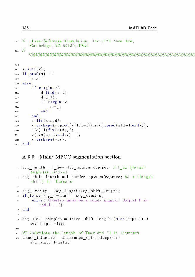
186 MATLAB Code
564 % Free Software Foundation , Inc . , 675 Mass Ave ,Cambridge , MA 02139 , USA.
565 %%%%%%%%%%%%%%%%%%%%%%%%%%%%%%%%%%%%%%%%%%%%%%%%%%%%%%%%%%%%%%%%%%%%%%%%%%%%%%%%%
566
567 s=s i z e ( x ) ;568 i f prod ( s )==1569 y=x570 e l s e571 i f narg in <3572 d=f i nd ( s>1) ;573 d=d (1) ;574 i f nargin<2575 n= [ ] ;576 end577 end578 y=f f t (x , n , d) ;579 y=reshape (y , prod ( s ( 1 : d−1) ) , s (d) , prod ( s (d+1:end ) ) ) ;580 s (d)=1+f i x ( s (d) /2) ;581 y ( : , s (d )+1:end , : ) = [ ] ;582 y=reshape (y , s ) ;583 end
A.5.5 Main: MFCC segmentation section
1 seg_length = l_aw∗mfcc_opts . mfccprsec ; % l_aw ( l engthana l y s i s window)
2 seg_shi f t_length = l_s∗mfcc_opts . mfccprsec ; %l_s ( l engths h i f t ) in Lasse ' s
3
4 seg_overlap = seg_length / seg_shi f t_length ;5 i f ( f l o o r ( seg_overlap )~=seg_overlap )6 e r r o r ( ' Overlap must be a whole number ! Adjust l_aw
and l_s . ' )7 end8
9 seg_start_samples = 1 : seg_shi f t_length : ( s i z e ( ceps , 1 )−(seg_length−1) ) ;
10
11 %% Calcu la te the l ength o f Tmax and Ti in segments12 Tmax_influence = Tmax∗mfcc_opts . mfccprsec /
seg_shi f t_length ;
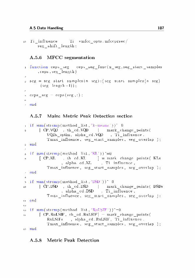
A.5 Data Handling 187
13 Ti_inf luence = Ti ∗mfcc_opts . mfccprsec /seg_shi f t_length ;
A.5.6 MFCC segmentation
1 f unc t i on ceps_seg = ceps_seg_func ( n_seg , seg_start_samples, ceps , seg_length )
2
3 seg = seg_start_samples ( n_seg ) : ( seg_start_samples ( n_seg )+(seg_length−1) ) ;
4
5 ceps_seg = ceps ( seg , : ) ;6
7 end
A.5.7 Main: Metric Peak Detection section
1 i f sum( strcmp (method_list , ' k−means ' ) )~=02 [ CP.VQD , th_cd .VQD ] = mark_change_points (
VQDs_optim , alpha_cd .VQD , Ti_inf luence ,Tmax_influence , seg_start_samples , seg_overlap ) ;
3 end4
5 i f sum( strcmp (method_list , 'KL ' ) )~=06 [ CP.KL , th_cd .KL ] = mark_change_points ( KLs
, alpha_cd .KL , Ti_inf luence ,Tmax_influence , seg_start_samples , seg_overlap ) ;
7 end8
9 i f sum( strcmp (method_list , 'DSD ' ) )~=010 [ CP.DSD , th_cd .DSD ] = mark_change_points ( DSDs
, alpha_cd .DSD , Ti_inf luence ,Tmax_influence , seg_start_samples , seg_overlap ) ;
11 end12
13 i f sum( strcmp (method_list , 'RuLSIF ' ) )~=014 [ CP. RuLSIF , th_cd . RuLSIF ] = mark_change_points (
RuLSIFs , alpha_cd . RuLSIF , Ti_inf luence ,Tmax_influence , seg_start_samples , seg_overlap ) ;
15 end
A.5.8 Metric Peak Detection

188 MATLAB Code
1 f unc t i on [ CP, th_cd ] = mark_change_points ( metric_data ,alpha , Ti_inf luence , Tmax_influence ,
seg_start_samples , seg_overlap )2 %% Calcu la te VQD_n, avr & th_cd , n ( Lasse ' s r epo r t page 62)3
4 movingavg = moving (metric_data ,2∗Tmax_influence+1) ; %c a l c u l a t e moving average with begin and end phaseinc luded
5
6 th_cd = alpha ∗movingavg ;7
8 %% Find change−po in t s9
10 CP = ze ro s ( l ength ( seg_start_samples )−seg_overlap , 1 ) ;11 f o r n_seg = 1 : l ength ( metric_data )12 i f ( metric_data ( n_seg )>th_cd ( n_seg ) )13 %take s t a r t and end s t ep s in to account14 i f ( n_seg − Ti_inf luence < 1)15 Ti_influenced_segments = 1 : n_seg+Ti_inf luence
;16 e l s e i f ( n_seg + Ti_inf luence > length ( metric_data
) )17 Ti_influenced_segments = n_seg−Ti_inf luence :
l ength ( metric_data ) ;18 e l s e19 Ti_influenced_segments = n_seg−Ti_inf luence :
n_seg+Ti_inf luence ;20 end21 %f ind l a r g e s t l o c a l peak22 i f ( metric_data ( n_seg )==max(metric_data (
Ti_influenced_segments ) ) )23 CP(n_seg ) = 1 ;24 e l s e25 CP(n_seg ) = 0 ;26 end27 end28 end29
30 end
A.6 Miscellaneous

A.6 Miscellaneous 189
1 f unc t i on value = compare_segments ( segment_A , segment_B ,method )
2
3 i f strcmp ( 'k−means ' , method )4
5 segment_A = segment_A ( : , 1 : 1 2 ) ;6 segment_B = segment_B ( : , 1 : 1 2 ) ;7 g l oba l K8 K_FAC = K9
10 kmeans_opts = s t a t s e t ( ' MaxIter ' ,10000) ;11
12 warning ( ' o f f ' , ' a l l ' ) ;13 [~ , prev ious_cent ro ids ] = kmeans ( segment_A ,K_FAC, '
Options ' , kmeans_opts , ' emptyaction ' , ' s i n g l e t on ' , 'on l inephase ' , ' o f f ' ) ;
14 [~ , next_centro ids ] = kmeans ( segment_B ,K_FAC, 'Options ' , kmeans_opts , ' emptyaction ' , ' s i n g l e t on ' , 'on l inephase ' , ' o f f ' ) ;
15 warning ( ' on ' , ' a l l ' ) ;16 %value (n) = (VQD_optim( prev ious_centro ids , segment_B)
+ VQD_optim( next_centroids , segment_A) ) /2 ;17 value = (VQD_optim( prev ious_centro ids , next_centro ids )
+ VQD_optim( next_centroids , p rev ious_cent ro ids ) )/2 ;
18 e l s e i f strcmp ( 'RuLSIF ' , method )19
20 alpha = . 1 ; % Smoothing parameter21 s igma_l i s t = 0 . 2 : 0 . 4 : 2 ; % Kernel Width22 lambda_list = −6:1:−2; % Regura l i z a t i on parameter23 k_folds = 5 ;24
25 addpath ( ' RuLSIF_change_detection ' )26 addpath ( ' RuLSIF_change_detection\RuLSIF ' )27
28 [ score1 , ~ , ~ , ~ , ~] = RelULSIF ( segment_A ' , segment_B' , [ ] , [ ] , alpha , k_folds , s igma_l ist , lambda_list ) ;
29 [ score2 , ~ , ~ , ~ , ~] = RelULSIF ( segment_B ' , segment_A' , [ ] , [ ] , alpha , k_folds , s igma_l ist , lambda_list ) ;
30
31 value = sco re1 + sco re2 ;32 e l s e i f strcmp ( 'DSD ' , method )33 previous_sigma = cov ( segment_A) ' ;34 next_sigma = cov ( segment_B) ' ;

190 MATLAB Code
35
36 value = DSD( previous_sigma , next_sigma ) ;37 e l s e i f strcmp ( 'KL ' , method )38 previous_sigma = cov ( segment_A) ' ;39 previous_mu = mean( segment_A) ' ;40 next_sigma = cov ( segment_B) ' ;41 next_mu = mean( segment_B) ' ;42
43 value = KL( previous_sigma , next_sigma , previous_mu ,next_mu) ;
44 e l s e i f strcmp ( 'BIC ' , method )45
46 previous_segment = segment_A ;47 next_segment = segment_B ;48
49 s igma_le f t = cov ( previous_segment ) ;50 sigma_right = cov ( next_segment ) ;51 s igma_ful l = cov ( [ previous_segment ; next_segment ] ) ;52 N1 = s i z e ( previous_segment , 1 ) ;53 N2 = s i z e ( next_segment , 1 ) ;54 N = N1+N2 ;55 R = N∗ l og ( det ( s igma_ful l ) )−N1∗ l og ( det ( s igma_le f t ) )−N2
∗ l og ( det ( sigma_right ) ) ;56 d = s i z e ( previous_segment , 2 ) ;57 P = 1/2∗(d+1/2∗d∗(d+1) ) ∗ l og (N) ;58 lambda = 1 ; %BIC d e f i n i t i o n59 BIC = R−lambda∗P;60
61 value = BIC ;62 e l s e i f strcmp ( 'ICR ' , method )63
64 sigma_A = cov ( segment_A) ;65 sigma_B = cov ( segment_B) ;66 s igma_ful l = cov ( [ segment_A ; segment_B ] ) ;67 N1 = s i z e ( segment_A , 1 ) ;68 N2 = s i z e ( segment_B , 1 ) ;69 N = N1+N2 ;70
71 ICR = 1/2∗ l og ( det ( s igma_ful l ) ) − . . .72 1/N∗1/2∗(N1∗ l og ( det ( sigma_A) )+N2∗ l og ( det ( sigma_B)
) ) ;73
74 d = s i z e ( segment_A , 2 ) ;75 P = 1/2∗(d+1/2∗d∗(d+1) ) ∗ l og (N) ;

A.6 Miscellaneous 191
76 lambda = 1 ; % from paper (A Robust Stopping Cr i t e r i onf o r Agglomerative H i e r a r c h i c a l C lu s t e r i ng in a
Speaker D i a r i z a t i on System )77 value = ICR−lambda∗P;78 e l s e79 e r r o r ( [ 'Unknown segment comparison method : " ' method
' " . ' ] )80 end81
82 end
A.6.1 F-measure
1 alpha_f_measure = 0 . 5 ;2 methods = f i e ldnames (CP) ;3 CP_TP = ze ro s ( numel (methods ) ,1 ) ;4
5 f o r n_method = 1 : numel (methods )6 CP_temp = x_axis (CP. ( methods{n_method})==1) ;7 f o r n_CP = 1 : numel ( changepoints_true )8 i f sum( (CP_temp−Ti /2) < changepoints_true (n_CP) &
changepoints_true (n_CP) < (CP_temp+Ti /2) )~=0;9 CP_TP(n_method) = CP_TP(n_method) + 1 ;10 end11 end12 RCL. ( methods{n_method}) = CP_TP(n_method) /numel (
changepoints_true ) ;13 PRC. ( methods{n_method}) = CP_TP(n_method) /numel (
CP_temp ) ;14 F_measure . ( methods{n_method}) = (RCL. ( methods{
n_method}) ∗PRC. ( methods{n_method}) ) /(alpha_f_measure∗RCL. ( methods{n_method})+(1−alpha_f_measure ) ∗PRC. ( methods{n_method}) ) ;
15 end
A.6.2 SCD Main Wrapper
1 f unc t i on out = Main_wrapper (method , alpha_cd_input ,alpha_fac_input , change_points , fac_method )
2

192 MATLAB Code
3 method_list = {method } ;4
5 alpha_cd . ( structname ) = alpha_cd_input ;6 alpha_fac . ( structname ) = alpha_fac_input ;7
8 wrapper_ON = 1 ;9 Main10 c l e a r wrapper_ON11
12 out = F_measure . ( structname ) ;13
14 end
A.6.3 Principal Component Analysis
1 % Subtract the mean from the data2 % Y = bsxfun (@minus , ceps ' , mean( ceps ' ) ) ; %a l rdy done in
Feature ex t r a c t i on3
4 % Obtain the PCA so l u t i o n by doing a SVD of Y5 [U, S , V] = svd (PCA_input , ' econ ' ) ;6
7 % Compute the p r o j e c t i o n onto the p r i n c i p a l components8 Z = U∗S ;9
10 % Compute amount o f var i ance exp la ined by components11 rho = diag (S) .^2 . / sum( diag (S) .^2) ;
A.6.4 Receiver Operator Characteristics
1 f unc t i on [ rx , ry , area ] = rocarea ( Ztest , Ytest , f r a c )2 % func t i on [ rx , ry , area ] = rocarea ( Ztest , Ytest , f r a c )3 %
%%%%%%%%%%%%%%%%%%%%%%%%%%%%%%%%%%%%%%%%%%%%%%%%%%%%%%%%%%%%%%%%%%
4 % th i s func t i on f i n d s the ROC and the area under the5 % ROC fo r l a b e l s in YTEST6 % STEP 1 convert Y to 0−1 array7 %8 % INPUT

A.6 Miscellaneous 193
9 % Ztes t : va lue s to be ROC' ed10 % Ytest : "True" l a b e l s obta ined by th r e sho ld ing Ytest
at zero11 % f r a c : the f r a c o f f a l s e p o s i t i v e s f o r which the area
i s computed12 % OUTPUT13 % rx : Fa l se p o s i t i v e r a t e s14 % ry : True p o s i t i v e r a t e s15 % area : the area under the curve f o r rx < f r a c16 %
%%%%%%%%%%%%%%%%%%%%%%%%%%%%%%%%%%%%%%%%%%%%%%%%%%%%%%%%%%%%%%%%%%%
17 % Lars Kai Hansen , Technica l Un ive r s i ty o f Denmark , ( c )2004
18 %%%%%%%%%%%%%%%%%%%%%%%%%%%%%%%%%%%%%%%%%%%%%%%%%%%%%%%%%%%%%%%%%%%%
19
20 top=max( Ytest ) ;21 N=length ( Ytest ) ;22 y=ze ro s (N, 1 ) ;23 indy=f i nd ( Ytest >0) ;24 y ( indy )=1;25 Npos=sum(y ) ;26 Nneg=N−Npos ;27 %IZt e s t index f o r order Zte s t ( smal l f i r s t )28 [dummy, IZ t e s t ]= so r t (−Ztes t ) ;29 y=y( IZ t e s t ) ;30 % COMPUTE SENSITIVITY31 ry=cumsum(y ) ;32 % compute 1− s p e c i f i c i t y33 rx=(1:N)−ry ' ;34 %normal ize35 ry=ry/Npos ;36 rx=rx . /Nneg ;37 %whos38 % compute area f o r rx<f r a c39 index_max=max( f i nd ( rx<f r a c ) ) ;40 area=sum( ry ( 1 : ( index_max−1) ) ' . ∗ ( rx ( 2 : index_max )−rx ( 1 : (
index_max−1) ) ) ) / f r a c ;
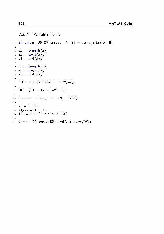
194 MATLAB Code
A.6.5 Welch's t-test
1 f unc t i on [ SE DF t s c o r e t95 f ] = ttest_mine (A, B)2
3 n1 = length (A) ;4 x1 = mean(A) ;5 s1 = std (A) ;6
7 n2 = length (B) ;8 x2 = mean(B) ;9 s2 = std (B) ;10
11 SE = sqr t ( s1^2/n1 + s2^2/n2 ) ;12
13 DF = (n1 − 1) + (n2 − 1) ;14
15 t s c o r e = abs ( ( ( x1 − x2 )−0)/SE) ;16
17 c i = 0 . 9 5 ;18 alpha = 1 − c i ;19 t95 = t inv (1−alpha /2 , DF) ;20
21 f = t cd f ( t s co re ,DF)−t cd f (− t s co re ,DF) ;

Bibliography
[1] Robert Alexander Adams and Christopher Essex. Calculus: a completecourse, volume 4. Addison-Wesley Don Mills, Ontario, 1995.
[2] Stanley C Ahalt, Ashok K Krishnamurthy, Prakoon Chen, and Douglas EMelton. Competitive learning algorithms for vector quantization. Neuralnetworks, 3(3):277�290, 1990.
[3] Peter Ahrendt, Anders Meng, and Jan Larsen. Decision time horizon formusic genre classi�cation using short time features. 2004.
[4] Jitendra Ajmera, Iain McCowan, and Hervé Bourlard. Robust speakerchange detection. Signal Processing Letters, IEEE, 11(8):649�651, 2004.
[5] SM Ali and Samuel D Silvey. A general class of coe�cients of divergenceof one distribution from another. Journal of the Royal Statistical Society.Series B (Methodological), pages 131�142, 1966.
[6] Daniel Aloise, Amit Deshpande, Pierre Hansen, and Preyas Popat. Np-hardness of euclidean sum-of-squares clustering. Machine Learning,75(2):245�248, 2009.
[7] Jeronimo Arenas-Garcia, Vanessa Gomez-Verdejo, and Aníbal RFigueiras-Vidal. New algorithms for improved adaptive convex combina-tion of lms transversal �lters. Instrumentation and Measurement, IEEETransactions on, 54(6):2239�2249, 2005.
[8] Christopher M Bishop and Nasser M Nasrabadi. Pattern recognition andmachine learning, volume 1. springer New York, 2006.

196 BIBLIOGRAPHY
[9] Christoph Boehm and Franz Pernkopf. E�ective metric-based speakersegmentation in the frequency domain. In Acoustics, Speech and SignalProcessing, 2009. ICASSP 2009. IEEE International Conference on, pages4081�4084. IEEE, 2009.
[10] Steven Boll. Suppression of acoustic noise in speech using spectral sub-traction. Acoustics, Speech and Signal Processing, IEEE Transactions on,27(2):113�120, 1979.
[11] Leon Bottou and Yoshua Bengio. Convergence properties of the k-meansalgorithms. In Advances in Neural Information Processing Systems 7.Citeseer, 1995.
[12] Markus M Breunig, Hans-Peter Kriegel, Raymond T Ng, and Jörg Sander.Lof: identifying density-based local outliers. In ACM Sigmod Record,volume 29, pages 93�104. ACM, 2000.
[13] Mike Brookes et al. Voicebox: Speech processing toolbox for matlab.Software, available [Mar. 2011] fromwww.ee.ic.ac.uk/hp/sta�/dmb/voicebox/voicebox.html, 1997.
[14] D Burton, J Shore, and J Buck. A generalization of isolated word recog-nition using vector quantization. In Acoustics, Speech, and Signal Pro-cessing, IEEE International Conference on ICASSP'83., volume 8, pages1021�1024. IEEE, 1983.
[15] David Byatt. Convergent variants of the nelder-mead algorithm. 2000.
[16] Jingdong Chen, Kuldip K Paliwal, and Satoshi Nakamura. Cepstrumderived from di�erentiated power spectrum for robust speech recognition.Speech Communication, 41(2):469�484, 2003.
[17] Shih-Sian Cheng and Hsin-Min Wang. A sequential metric-based audiosegmentation method via the bayesian information criterion. In INTER-SPEECH, 2003.
[18] Shih-Sian Cheng and Hsin-min Wang. Metric-seqdac: A hybrid approachfor audio segmentation. In Proc. International Conference on Spoken Lan-guage Processing, 2004.
[19] Stephen M Chu, Hao Tang, and Thomas S Huang. Fishervoice and semi-supervised speaker clustering. In Acoustics, Speech and Signal Processing,2009. ICASSP 2009. IEEE International Conference on, pages 4089�4092.IEEE, 2009.
[20] CoSound. A cognitive systems approach to enriched and action-able information from audio streams supported by the danish strate-gic research council, jan. 2012 � dec. 2015. More information online@http://www.cosound.dk/. Last checked, June 2013.

BIBLIOGRAPHY 197
[21] I. Csiszár. Information-type measures of di�erence of probability distri-butions and indirect observations. Studia Sci. Math. Hungar., 2:299�318,1967.
[22] Neil R Davis. Method for audio editing, July 12 1988. US Patent 4,757,540.
[23] Steven Davis and Paul Mermelstein. Comparison of parametric repre-sentations for monosyllabic word recognition in continuously spoken sen-tences. Acoustics, Speech and Signal Processing, IEEE Transactions on,28(4):357�366, 1980.
[24] Perrine Delacourt and Christian J Wellekens. Distbic: A speaker-basedsegmentation for audio data indexing. Speech communication, 32(1):111�126, 2000.
[25] John R Deller, John G Proakis, and John HL Hansen. Discrete-timeprocessing of speech signals. Ieee New York, NY, USA:, 2000.
[26] Qiang Du, Vance Faber, and Max Gunzburger. Centroidal voronoi tessel-lations: Applications and algorithms. SIAM review, 41(4):637�676, 1999.
[27] Brian Everitt and Anders Skrondal. The Cambridge dictionary of statis-tics, volume 4. Cambridge University Press Cambridge, 2002.
[28] JE Muñoz Expósito, N Ruiz Reyes, S Garcia Galán, and P Vera Candeas.Speech/music classi�cation based on distributed evolutionary fuzzy logicfor intelligent audio coding. In Pattern Recognition and Image Analysis,pages 556�563. Springer, 2007.
[29] Gunnar Fant. Analys av de svenska konsonantljuden: talets allmännasvängningsstruktur. LM Ericsson, 1949.
[30] Ling Feng. Speaker recognition. PhD thesis, Technical University of Den-mark, DTU, DK-2800 Kgs. Lyngby, Denmark, 2004.
[31] Ling Feng. English Language Speech Database for Speaker Recognition,ELSDSR, @http://www2.imm.dtu.dk. last checked, June 2013.
[32] Ling Feng, Andreas Brinch Nielsen, and Lars Kai Hansen. Vocal segmentclassi�cation in popular music. In ISMIR, pages 121�126, 2008.
[33] JA Nolazco Flores and SJ Young. Continuous speech recognition in noiseusing spectral subtraction and hmm adaptation. In Acoustics, Speech, andSignal Processing, 1994. ICASSP-94., 1994 IEEE International Confer-ence on, volume 1, pages I�409. IEEE, 1994.
[34] Edward W Forgy. Cluster analysis of multivariate data: e�ciency versusinterpretability of classi�cations. Biometrics, 21:768�769, 1965.

198 BIBLIOGRAPHY
[35] Mark JF Gales and Stephen J Young. Robust continuous speech recog-nition using parallel model combination. Speech and Audio Processing,IEEE Transactions on, 4(5):352�359, 1996.
[36] Todor Ganchev, Nikos Fakotakis, and George Kokkinakis. Comparativeevaluation of various mfcc implementations on the speaker veri�cationtask. In Proceedings of the SPECOM, volume 1, pages 191�194, 2005.
[37] John S. Garofolo. TIMIT Acoustic-Phonetic Continuous Speech Corpus,@http://www.ldc.upenn.edu/. Last checked, April 2013.
[38] D Geller, Reinhold Haeb-Umbach, and Hermann Ney. Improvements inspeech recognition for voice dialing in the car environment. In SpeechProcessing in Adverse Conditions, 1992.
[39] Allen Gersho and Robert M Gray. Vector quantization and signal com-pression. Springer, 1992.
[40] Robert Gray. Vector quantization. ASSP Magazine, IEEE, 1(2):4�29,1984.
[41] Donald D. Greenwood. Mailing list from 2009; discussion on bias inthe Mel scale due to Hysteresis e�ects, @http://lists.mcgill.ca/scripts/wa.exe?A2=ind0907d&L=auditory&P=389. Last checked, May 2013.
[42] Kyu Jeong Han and Shrikanth S Narayanan. A robust stopping criterionfor agglomerative hierarchical clustering in a speaker diarization system.In INTERSPEECH, pages 1853�1856. Citeseer, 2007.
[43] Lars Kai Hansen, Peter Ahrendt, and Jan Larsen. Towards cognitivecomponent analysis. 2005.
[44] Lars Kai Hansen, Christian Liisberg, and Peter Salamon. The error-rejecttradeo�. Open Systems & Information Dynamics, 4(2):159�184, 1997.
[45] Gunther Heidemann and Helge Ritter. E�cient vector quantization us-ing the wta-rule with activity equalization. Neural Processing Letters,13(1):17�30, 2001.
[46] Ramon E Henkel. Tests of signi�cance, volume 4. Sage, 1976.
[47] Hynek Hermansky and Nelson Morgan. Rasta processing of speech. Speechand Audio Processing, IEEE Transactions on, 2(4):578�589, 1994.
[48] Hynek Hermansky, Nelson Morgan, Aruna Bayya, and Phil Kohn. Com-pensation for the e�ect of the communication channel in auditory-likeanalysis of speech (rasta-plp). In Second European Conference on SpeechCommunication and Technology, 1991.
BIBLIOGRAPHY 199
[49] HG Hirsch, Peter Meyer, and Hans-Wilhelm Ruehl. Improved speechrecognition using high-pass �ltering of subband envelopes. In Eurospeech,volume 91, pages 413�416, 1991.
[50] Thomas Hofmann and Joachim M Buhmann. Competitive learning algo-rithms for robust vector quantization. Signal Processing, IEEE Transac-tions on, 46(6):1665�1675, 1998.
[51] Peter J Huber. Robust statistics. Springer, 2011.
[52] Anil Jain and Douglas Zongker. Feature selection: Evaluation, appli-cation, and small sample performance. Pattern Analysis and MachineIntelligence, IEEE Transactions on, 19(2):153�158, 1997.
[53] Jesper H. Jensen, Anders Meng, Elvis Ramonovic, Kaare B. Petersen,Mads G. Christensen, Sigurdur Sigurdsson, and Tue Lehn-Schiøler. Intel-ligent Sound Processing Toolbox, ISP. Available online@http://kom.aau.dk/project/isound/. Last checked, May 2013.
[54] Kasper W Jørgensen, Lasse Mølgaard, and Lars Kai Hansen. Unsuper-vised speaker change detection for broadcast news segmentation. 2006.
[55] Kasper Winther Jørgensen and Lasse Lohilahti Mølgaard. Tools for au-tomatic audio indexing. PhD thesis, Technical University of Denmark,DTU, DK-2800 Kgs. Lyngby, Denmark, 2006.
[56] Biing-Hwang Juang and Mazin G Rahim. Signal bias removal by maxi-mum likelihood estimation for robust telephone speech recognition. Speechand Audio Processing, IEEE Transactions on, 4(1):19, 1996.
[57] Takafumi Kanamori, Taiji Suzuki, and Masashi Sugiyama. Statisticalanalysis of kernel-based least-squares density-ratio estimation. MachineLearning, 86(3):335�367, 2012.
[58] Takafumi Kanamori, Taiji Suzuki, and Masashi Sugiyama. Computationalcomplexity of kernel-based density-ratio estimation: a condition numberanalysis. Machine Learning, 90(3):431�460, 2013.
[59] Yoshinobu Kawahara and Masashi Sugiyama. Sequential change-pointdetection based on direct density-ratio estimation. Statistical Analysisand Data Mining, 5(2):114�127, 2012.
[60] H Kim, Daniel Ertelt, and Thomas Sikora. Hybrid speaker-based segmen-tation system using model-level clustering. In Proc. 2005 IEEE Int. Conf.Acoustics, Speech, and Signal Processing, volume 1, pages 745�748, 2005.
[61] Tomi Kinnunen, TEEMU KILPELÄINEN, and Pasi FrÄnti. Comparisonof clustering algorithms in speaker identi�cation. dim, 1:2, 2000.
200 BIBLIOGRAPHY
[62] Tomi Kinnunen and Haizhou Li. An overview of text-independent speakerrecognition: From features to supervectors. Speech communication,52(1):12�40, 2010.
[63] Teuvo Kohonen. Self-organizing maps, volume 30. Springer, 2001.
[64] Margarita Kotti, Emmanouil Benetos, and Constantine Kotropoulos. Au-tomatic speaker change detection with the bayesian information criterionusing mpeg-7 features and a fusion scheme. In Circuits and Systems, 2006.ISCAS 2006. Proceedings. 2006 IEEE International Symposium on, pages4�pp. IEEE, 2006.
[65] Margarita Kotti, Emmanouil Benetos, and Costas Kotropoulos. Com-putationally e�cient and robust bic-based speaker segmentation. Audio,Speech, and Language Processing, IEEE Transactions on, 16(5):920�933,2008.
[66] Margarita Kotti, Lu�s Gustavo PM Martins, Emmanouil Benetos, Jaime SCardoso, and Constantine Kotropoulos. Automatic speaker segmentationusing multiple features and distance measures: a comparison of three ap-proaches. In Multimedia and Expo, 2006 IEEE International Conferenceon, pages 1101�1104. IEEE, 2006.
[67] E Kreyszig. Advanced engineering mathematics, 9th ednwiley. New York,NY, USA, 2005.
[68] Daben Liu Francis Kubala. Fast speaker change detection for broadcastnews transcription and indexing. 1999.
[69] Solomon Kullback and Richard A Leibler. On information and su�ciency.The Annals of Mathematical Statistics, 22(1):79�86, 1951.
[70] Je�rey C Lagarias, James A Reeds, Margaret H Wright, and Paul EWright. Convergence properties of the nelder�mead simplex method inlow dimensions. SIAM Journal on Optimization, 9(1):112�147, 1998.
[71] Michael S Lewicki. E�cient coding of natural sounds. Nature neuro-science, 5(4):356�363, 2002.
[72] Robert Michael Lewis, Virginia Torczon, and Michael W Trosset. Directsearch methods: then and now. Journal of Computational and AppliedMathematics, 124(1):191�207, 2000.
[73] Yoseph Linde, Andres Buzo, and Robert Gray. An algorithm for vectorquantizer design. Communications, IEEE Transactions on, 28(1):84�95,1980.

BIBLIOGRAPHY 201
[74] Song Liu. Prof. Sugiyama's webpage, @http://www.cs.titech.ac.jp. Lastchecked, April 2013.
[75] Song Liu, Makoto Yamada, Nigel Collier, and Masashi Sugiyama. Change-point detection in time-series data by relative density-ratio estimation.Neural Networks, 2013.
[76] Stuart Lloyd. Least squares quantization in pcm. Information Theory,IEEE Transactions on, 28(2):129�137, 1982.
[77] Lie Lu and Hong-Jiang Zhang. Speaker change detection and tracking inreal-time news broadcasting analysis. In Proceedings of the tenth ACMinternational conference on Multimedia, pages 602�610. ACM, 2002.
[78] Lie Lu and Hong-Jiang Zhang. Unsupervised speaker segmentationand tracking in real-time audio content analysis. Multimedia systems,10(4):332�343, 2005.
[79] Lie Lu, Hong-Jiang Zhang, and Hao Jiang. Content analysis for audio clas-si�cation and segmentation. Speech and Audio Processing, IEEE Trans-actions on, 10(7):504�516, 2002.
[80] J Makhoul and L Cosell. Lpcw: An lpc vocoder with linear predictivespectral warping. In Acoustics, Speech, and Signal Processing, IEEE In-ternational Conference on ICASSP'76., volume 1, pages 466�469. IEEE,1976.
[81] Amit S Malegaonkar, Aladdin M Ariyaeeinia, and Perasiriyan Sivaku-maran. E�cient speaker change detection using adapted gaussian mixturemodels. Audio, Speech, and Language Processing, IEEE Transactions on,15(6):1859�1869, 2007.
[82] MATLAB. Statistics Toolbox - Exploratory Data Analysis - ClusterAnalysis - K-Means Clustering, @http://www.mathworks.se/help/stats/kmeans.html. Last checked, July 2013.
[83] Martin F McKinney and Jeroen Breebaart. Features for audio and musicclassi�cation. In ISMIR, volume 3, pages 151�158, 2003.
[84] Sylvain Meignier, Daniel Moraru, Corinne Fredouille, Jean-FrancoisBonastre, and Laurent Besacier. < i> step-by-step</i> and< i> inte-grated</i> approaches in broadcast news speaker diarization. ComputerSpeech & Language, 20(2):303�330, 2006.
[85] Hugo Meinedo and Joao Neto. Audio segmentation, classi�cation andclustering in a broadcast news task. In Acoustics, Speech, and Signal Pro-cessing, 2003. Proceedings.(ICASSP'03). 2003 IEEE International Con-ference on, volume 2, pages II�5. IEEE, 2003.

202 BIBLIOGRAPHY
[86] Mohammad H Moattar and Mohammad M Homayounpour. A reviewon speaker diarization systems and approaches. Speech Communication,54(10):1065�1103, 2012.
[87] LL Mølgaard, KW Jørgensen, and Lars Kai Hansen. Castsearch-contextbased spoken document retrieval. In Acoustics, Speech and Signal Process-ing, 2007. ICASSP 2007. IEEE International Conference on, volume 4,pages IV�93. IEEE, 2007.
[88] Pedro J Moreno, Bhiksha Raj, and Richard M Stern. A vector tay-lor series approach for environment-independent speech recognition. InAcoustics, Speech, and Signal Processing, 1996. ICASSP-96. ConferenceProceedings., 1996 IEEE International Conference on, volume 2, pages733�736. IEEE, 1996.
[89] Omer Mohsin Mubarak, Eliathamby Ambikairajah, and Julien Epps.Analysis of an mfcc-based audio indexing system for e�cient coding ofmultimedia sources. In ISSPA, pages 619�622, 2005.
[90] Hiroshi Nakagawa and Tatsunori Mori. Automatic term recognition basedon statistics of compound nouns and their components. Terminology,9(2):201�219, 2003.
[91] John A Nelder and Roger Mead. A simplex method for function mini-mization. The computer journal, 7(4):308�313, 1965.
[92] Kazumi Ohkura, Masahide Sugiyama, and Shigeki Sagayama. Speakeradaptation based on transfer vector �eld smoothing with continuous mix-ture density hmms. In Second International Conference on Spoken Lan-guage Processing, 1992.
[93] Alan V Oppenheim. Superposition in a class of nonlinear systems. Tech-nical report, DTIC Document, 1965.
[94] Alan V Oppenheim and Ronald W Schafer. From frequency to quefrency:A history of the cepstrum. Signal Processing Magazine, IEEE, 21(5):95�106, 2004.
[95] Karl Pearson. X. on the criterion that a given system of deviations fromthe probable in the case of a correlated system of variables is such that itcan be reasonably supposed to have arisen from random sampling. TheLondon, Edinburgh, and Dublin Philosophical Magazine and Journal ofScience, 50(302):157�175, 1900.
[96] R Plomp, LCW Pols, and JP Van der Geer. Dimensional analysis of vowelspectra. Journal of Acoustical Society of America, 41:707�712, 1967.

BIBLIOGRAPHY 203
[97] Louis CW Pols. Spectral analysis and identi�cation of dutch vowels inmonosyllabic words. 1977.
[98] Dimitrie C Popescu and Ilija Zeljkovic. Kalman �ltering of colored noisefor speech enhancement. In Acoustics, Speech and Signal Processing, 1998.Proceedings of the 1998 IEEE International Conference on, volume 2,pages 997�1000. IEEE, 1998.
[99] John G Proakis. Digital Signal Processing: Principles, Algorithms, andApplications, 4/e. Pearson Education India, 2007.
[100] Lawrence Rabiner and Biing-Hwang Juang. Fundamentals of speech recog-nition. 1993.
[101] Douglas A Reynolds. Channel robust speaker veri�cation via featuremapping. In Acoustics, Speech, and Signal Processing, 2003. Proceed-ings.(ICASSP'03). 2003 IEEE International Conference on, volume 2,pages II�53. IEEE, 2003.
[102] Walter Rudin. Principles of mathematical analysis, volume 3. McGraw-Hill New York, 1964.
[103] Franklin E Satterthwaite. An approximate distribution of estimates ofvariance components. Biometrics bulletin, 2(6):110�114, 1946.
[104] Burr Settles. Active learning literature survey. University of Wisconsin,Madison, 2010.
[105] Matthew A Siegler, Uday Jain, Bhiksha Raj, and Richard M Stern. Auto-matic segmentation, classi�cation and clustering of broadcast news audio.In Proc. DARPA Broadcast News Workshop, page 11, 1997.
[106] Sigurdur Sigurdsson, Kaare Brandt Petersen, and Tue Lehn-Schiøler. Melfrequency cepstral coe�cients: An evaluation of robustness of mp3 en-coded music. 2006.
[107] Rohit Sinha, Sue E Tranter, Mark JF Gales, and Philip C Woodland. Thecambridge university march 2005 speaker diarisation system. In INTER-SPEECH, pages 2437�2440, 2005.
[108] F Soong, A Rosenberg, L Rabiner, and B Juang. A vector quantiza-tion approach to speaker recognition. In Acoustics, Speech, and SignalProcessing, IEEE International Conference on ICASSP'85., volume 10,pages 387�390. IEEE, 1985.
[109] Stanley S Stevens. On the psychophysical law. Psychological review,64(3):153, 1957.

204 BIBLIOGRAPHY
[110] Stanley S Stevens and JOHN Volkmann. The relation of pitch to fre-quency: A revised scale. The American Journal of Psychology, 53(3):329�353, 1940.
[111] Masashi Sugiyama, Taiji Suzuki, and Takafumi Kanamori. Density-ratio matching under the bregman divergence: a uni�ed framework ofdensity-ratio estimation. Annals of the Institute of Statistical Mathemat-ics, 64(5):1009�1044, 2012.
[112] Masashi Sugiyama, Taiji Suzuki, Shinichi Nakajima, Hisashi Kashima,Paul von Bünau, and Motoaki Kawanabe. Direct importance estimationfor covariate shift adaptation. Annals of the Institute of Statistical Math-ematics, 60(4):699�746, 2008.
[113] Pang-Ning Tan et al. Introduction to data mining. Pearson EducationIndia, 2007.
[114] SE Tranter, K Yu, G Everinann, and PC Woodland. Generating andevaluating segmentations for automatic speech recognition of conversa-tional telephone speech. In Acoustics, Speech, and Signal Processing, 2004.Proceedings.(ICASSP'04). IEEE International Conference on, volume 1,pages I�753. IEEE, 2004.
[115] Alain Tritschler and Ramesh A Gopinath. Improved speaker segmenta-tion and segments clustering using the bayesian information criterion. InEurospeech, volume 99, pages 679�682, 1999.
[116] Saeed V Vaseghi and Ben P Milner. Noise compensation methods forhidden markov model speech recognition in adverse environments. Speechand Audio Processing, IEEE Transactions on, 5(1):11�21, 1997.
[117] William N Venables, Brian D Ripley, and WN Venables. Modern appliedstatistics with S-PLUS, volume 250. Springer-verlag New York, 1994.
[118] Olli Viikki and Kari Laurila. Cepstral domain segmental feature vectornormalization for noise robust speech recognition. Speech Communication,25(1):133�147, 1998.
[119] Dong Wang, Lie Lu, and Hong-Jiang Zhang. Speech segmentation with-out speech recognition. In Acoustics, Speech, and Signal Processing, 2003.Proceedings.(ICASSP'03). 2003 IEEE International Conference on, vol-ume 1, pages I�468. IEEE, 2003.
[120] Bernard L Welch. The generalization ofstudent's' problem when severaldi�erent population variances are involved. Biometrika, 34(1/2):28�35,1947.

BIBLIOGRAPHY 205
[121] PC Woodland, MJF Gales, and D Pye. Improving environmental ro-bustness in large vocabulary speech recognition. In Acoustics, Speech,and Signal Processing, 1996. ICASSP-96. Conference Proceedings., 1996IEEE International Conference on, volume 1, pages 65�68. IEEE, 1996.
[122] Chung-Hsien Wu and Chia-Hsin Hsieh. Multiple change-point audio seg-mentation and classi�cation using an mdl-based gaussian model. Audio,Speech, and Language Processing, IEEE Transactions on, 14(2):647�657,2006.
[123] Ziyou Xiong, Regunathan Radhakrishnan, Ajay Divakaran, and Thomas SHuang. Comparing mfcc and mpeg-7 audio features for feature extrac-tion, maximum likelihood hmm and entropic prior hmm for sports audioclassi�cation. In Acoustics, Speech, and Signal Processing, 2003. Pro-ceedings.(ICASSP'03). 2003 IEEE International Conference on, volume 5,pages V�628. IEEE, 2003.
[124] Min Xu, Ling-Yu Duan, Jianfei Cai, Liang-Tien Chia, Changsheng Xu,and Qi Tian. Hmm-based audio keyword generation. In Advances inMultimedia Information Processing-PCM 2004, pages 566�574. Springer,2005.
[125] Makoto Yamada, Taiji Suzuki, Takafumi Kanamori, Hirotaka Hachiya,and Masashi Sugiyama. Relative density-ratio estimation for robust dis-tribution comparison. arXiv preprint arXiv:1106.4729, 2011.
[126] Arthur Zimek, Erich Schubert, and Hans-Peter Kriegel. A survey on unsu-pervised outlier detection in high-dimensional numerical data. StatisticalAnalysis and Data Mining, 5(5):363�387, 2012.