Efficient Moment-Based Inference of Admixture Parameters

Article

FastT

rack

Efficient Moment-Based Inference of Admixture Parametersand Sources of Gene FlowMark Lipson,y ,1 Po-Ru Loh,y ,1 Alex Levin,1 David Reich,2,3 Nick Patterson,2 and Bonnie Berger*,1,2

1Department of Mathematics and Computer Science and Artificial Intelligence Laboratory, Massachusetts Institute of Technology2Broad Institute, Cambridge, Massachusetts3Department of Genetics, Harvard Medical SchoolyThese authors contributed equally to this work.

*Corresponding author: E-mail: [email protected].

Associate editor: John Novembre

Abstract

The recent explosion in available genetic data has led to significant advances in understanding the demographic historiesof and relationships among human populations. It is still a challenge, however, to infer reliable parameter valuesfor complicated models involving many populations. Here, we present MixMapper, an efficient, interactive methodfor constructing phylogenetic trees including admixture events using single nucleotide polymorphism (SNP) genotypedata. MixMapper implements a novel two-phase approach to admixture inference using moment statistics, first buildingan unadmixed scaffold tree and then adding admixed populations by solving systems of equations that expressallele frequency divergences in terms of mixture parameters. Importantly, all features of the model, including topology,sources of gene flow, branch lengths, and mixture proportions, are optimized automatically from the data and includeestimates of statistical uncertainty. MixMapper also uses a new method to express branch lengths in easily interpretabledrift units. We apply MixMapper to recently published data for Human Genome Diversity Cell Line Panel individualsgenotyped on a SNP array designed especially for use in population genetics studies, obtaining confident results for30 populations, 20 of them admixed. Notably, we confirm a signal of ancient admixture in European populations—including previously undetected admixture in Sardinians and Basques—involving a proportion of 20–40% ancientnorthern Eurasian ancestry.

Key words: admixture, human populations, genetic drift, moment statistics.

IntroductionThe most basic way to represent the evolutionary history of aset of species or populations is through a phylogenetic tree, amodel that in its strict sense assumes that there is no geneflow between populations after they have diverged (Cavalli-Sforza and Edwards 1967). In many settings, however, groupsthat have split from one another can still exchange geneticmaterial. This is certainly the case for human population his-tory, during the course of which populations have often di-verged only incompletely or diverged and subsequentlymixed again (Reich et al. 2009; Wall et al. 2009; Green et al.2010; Laval et al. 2010; Reich et al. 2010; Gravel et al. 2011;Patterson et al. 2012). To capture these more complicatedrelationships, previous studies have considered models allow-ing for continuous migration among populations (Wall et al.2009; Laval et al. 2010; Gravel et al. 2011) or have extendedsimple phylogenetic trees into admixture trees, in which pop-ulations on separate branches are allowed to remerge andform an admixed offspring population (Chikhi et al. 2001;Wang 2003; Reich et al. 2009; Sousa et al. 2009; Pattersonet al. 2012). Both of these frameworks, of course, still representsubstantial simplifications of true population histories,but they can help capture a range of new and interestingphenomena.

Several approaches have previously been used to buildphylogenetic trees incorporating admixture events fromgenetic data. First, likelihood methods (Chikhi et al. 2001;Wang 2003; Sousa et al. 2009) use a full probabilistic evolu-tionary model, which allows a high level of precision withthe disadvantage of greatly increased computational cost.Consequently, likelihood methods can in practice onlyaccommodate a small number of populations (Wall et al.2009; Laval et al. 2010; Gravel et al. 2011; Siren et al. 2011).Moreover, the tree topology must generally be specified inadvance, meaning that only parameter values can be inferredautomatically and not the arrangement of populations in thetree. By contrast, the moment-based methods of Reich et al.(2009) and Patterson et al. (2012) use only means and vari-ances of allele frequency divergences. Moments are simplerconceptually and especially computationally, and they allowfor more flexibility in model conditions. Their disadvantagescan include reduced statistical power and difficulties in de-signing precise estimators with desirable statistical properties(e.g., unbiasedness) (Wang 2003). Finally, a number of studieshave considered “phylogenetic networks,” which generalizetrees to include cycles and multiple edges between pairs ofnodes and can be used to model population histories involv-ing hybridization (Huson and Bryant 2006; Yu et al. 2012).

� The Author 2013. Published by Oxford University Press on behalf of the Society for Molecular Biology and Evolution.This is an Open Access article distributed under the terms of the Creative Commons Attribution Non-Commercial License(http://creativecommons.org/licenses/by-nc/3.0/), which permits non-commercial re-use, distribution, and reproduction in anymedium, provided the original work is properly cited. For commercial re-use, please contact [email protected] Open Access1788 Mol. Biol. Evol. 30(8):1788–1802 doi:10.1093/molbev/mst099 Advance Access publication May 24, 2013

by guest on July 14, 2013http://m

be.oxfordjournals.org/D

ownloaded from

http://mbe.oxfordjournals.org/

However, these methods also tend to be computationallyexpensive.

In this work, we introduce MixMapper, a new computa-tional tool that fits admixture trees by solving systems ofmoment equations involving the pairwise distance statisticf2 (Reich et al. 2009; Patterson et al. 2012), which is the averagesquared allele frequency difference between two populations.The theoretical expectation of f2 can be calculated in terms ofbranch lengths and mixture fractions of an admixture treeand then compared with empirical data. MixMapper can bethought of as a generalization of the qpgraph package(Patterson et al. 2012), which takes as input genotype data,along with a proposed arrangement of admixed and unad-mixed populations, and returns branch lengths and mixturefractions that produce the best fit to allele frequency momentstatistics measured on the data. MixMapper, by contrast,performs the fitting in two stages, first constructing an unad-mixed scaffold tree via neighbor-joining and then automati-cally optimizing the placement of admixed populationsonto this initial tree. Thus, no topological relationshipsamong populations need to be specified in advance.

Our method is similar in spirit to the independently de-veloped TreeMix package (Pickrell and Pritchard 2012). LikeMixMapper, TreeMix builds admixture trees from second mo-ments of allele frequency divergences, although it does so viaa composite likelihood maximization approach made tracta-ble with a multivariate normal approximation. Procedurally,TreeMix initially fits a full set of populations as an unadmixedtree, and gene flow edges are added sequentially to accountfor the greatest errors in the fit (Pickrell and Pritchard 2012).This format makes TreeMix well suited to handling very largetrees: the entire fitting process is automated and can includearbitrarily many admixture events simultaneously. In contrast,MixMapper begins with a carefully screened unadmixed scaf-fold tree to which admixed populations are added with best-fitting parameter values, an interactive design that enablesprecise modeling of particular populations of interest.

We use MixMapper to model the ancestral relationshipsamong 52 populations from the CEPH-Human GenomeDiversity Cell Line Panel (HGDP) (Rosenberg et al. 2002; Liet al. 2008) using recently published data from a new, specially

ascertained single nucleotide polymorphism (SNP) array de-signed for population genetics applications (Keinan et al.2007; Patterson et al. 2012). Previous studies of these popu-lations have built simple phylogenetic trees (Li et al. 2008;Siren et al. 2011), identified a substantial number of admixedpopulations with likely ancestors (Patterson et al. 2012), andconstructed a large-scale admixture tree (Pickrell andPritchard 2012). Here, we add an additional level of quantita-tive detail, obtaining best-fit admixture parameters withbootstrap error estimates for 30 HGDP populations, ofwhich 20 are admixed. The results include, most notably, asignificant admixture event (Patterson et al. 2012) in the his-tory of all sampled European populations, among themSardinians and Basques.

New ApproachesThe central problem we consider is as follows: given an arrayof SNP data sampled from a set of individuals grouped bypopulation, what can we infer about the admixture historiesof these populations using simple statistics that are functionsof their allele frequencies? Methodologically, the MixMapperworkflow (fig. 1) proceeds as follows. We begin by computingf2 distances between all pairs of study populations, fromwhich we construct an unadmixed phylogenetic subtree toserve as a scaffold for subsequent mixture fitting. The choiceof populations for the scaffold is done via initial filtering ofpopulations that are clearly admixed according to the three-population test (Reich et al. 2009; Patterson et al. 2012), fol-lowed by selection of a subtree that is approximately additivealong its branches, as is expected in the absence of admixture(Materials and Methods and supplementary text S1,Supplementary Material online, for full details).

Next, we expand the model to incorporate admixtures byattempting to fit each population not in the scaffold as amixture between some pair of branches of the scaffold.Putative admixtures imply algebraic relations among f2 statis-tics, which we test for consistency with the data, allowing usto identify likely sources of gene flow and estimate mixtureparameters (fig. 2; supplementary text S1, SupplementaryMaterial online). After determining likely two-way admixtureevents, we further attempt to fit remaining populations as

Phase 2: Admixture fitting

• Two-way mixture fitting• Three-way mixture fitting• Conversion to drift units

Phase 1: Unadmixed scaffoldtree construction

• Unadmixed population filtering(f3-statistics > 0)

• Unadmixed subset selection(ranking by f2-additivity)

• Scaffold tree building(neighbor joining) Bootstrap resampling

FIG. 1. MixMapper workflow. MixMapper takes as input an array of SNP calls annotated with the population to which each individual belongs. Themethod then proceeds in two phases, first building a tree of (approximately) unadmixed populations and then attempting to fit the remainingpopulations as admixtures. In the first phase, MixMapper produces a ranking of possible unadmixed trees in order of deviation from f2-additivity; basedon this list, the user selects a tree to use as a scaffold. In the second phase, MixMapper tries to fit remaining populations as two- or three-way mixturesbetween branches of the unadmixed tree. In each case, MixMapper produces an ensemble of predictions via bootstrap resampling, enabling confidenceestimation for inferred results.

1789

Efficient Moment-Based Inference of Admixture Parameters . doi:10.1093/molbev/mst099 MBE by guest on July 14, 2013


Dow

nloaded from

http://mbe.oxfordjournals.org/lookup/suppl/doi:10.1093/molbev/mst099/-/DC1






three-way mixtures involving the inferred two-way mixedpopulations, by similar means. Finally, we use a new formulato convert the f2 tree distances into absolute drift units(supplementary text S2, Supplementary Material online).Importantly, we apply a bootstrap resampling scheme(Efron 1979; Efron and Tibshirani 1986) to obtain ensemblesof predictions, rather than single values, for all model vari-ables. This procedure allows us to determine confidence in-tervals for parameter estimates and guard against overfitting.For a data set on the scale of the HGDP, after initial setup timeon the order of an hour, MixMapper determines the best-fitadmixture model for a chosen population in a few seconds,enabling real-time interactive investigation.

Results

Simulations

To test the inference capabilities of MixMapper on popula-tions with known histories, we ran it on two data sets gen-erated with the coalescent simulator ms (Hudson 2002) anddesigned to have similar parameters to our human data. Inboth cases, we simulated 500 regions of 500 kb each for 25 dip-loid individuals per population, with an effective populationsize of 5,000 or 10,000 per population, a mutation rate of0:5� 10�8 per base per generation (intentionally low so asnot to create unreasonably many SNPs), and a recombinationrate of 10�8 per base per generation. Full ms commandscan be found in Materials and Methods. We ascertainedSNPs present at minor allele frequency 0.05 or greater in anoutgroup population and then removed that populationfrom the analysis.

For the first admixture tree, we simulated six nonoutgrouppopulations, with one of them, pop6, admixed (fig. 3A).Applying MixMapper, no admixtures were detected withthe three-population test, but the most additive subsetwith at least five populations excluded pop6 (max deviationfrom additivity 2:0� 10�4 vs. second-best 7:7� 10�4; see

Materials and Methods), so we used this subset as the scaffoldtree. We then fit pop6 as admixed, and MixMapper recoveredthe correct gene flow topology with 100% confidence andinferred the other parameters of the model quite accurately(fig. 3B; supplementary table S1, Supplementary Materialonline). For comparison, we also analyzed the same datawith TreeMix and again obtained accurate results (fig. 3C).

For the second test, we simulated a complex admixturescenario involving 10 nonoutgroup populations, with sixunadmixed and four admixed (fig. 3D). In this example,pop4 is recently admixed between pop3 and pop5, butover a continuous period of 40 generations. Meanwhile,pop8, pop9, and pop10 are all descended from older admix-ture events, which are similar but with small variations (lowermixture fraction in pop9, 40-generation continuous gene flowin pop10, and subsequent pop2-related admixture intopop8). In the first phase of MixMapper, the recently admixedpop4 and pop8 were detected with the three-population test.From among the other eight populations, a scaffold treeconsisting of pop1, pop2, pop3, pop5, pop6, and pop7 pro-vided thorough coverage of the data set and was moreadditive (max deviation 3:5� 10�4) than the second-best six-population scaffold (5:4� 10�4) and the bestseven-population scaffold (1:2� 10�3). Using this scaffold,MixMapper returned very accurate and high-confidence fitsfor the remaining populations (fig. 3E; supplementary tableS1, Supplementary Material online), with the correct geneflow topologies inferred with 100% confidence for pop4and pop10, 98% confidence for pop9, and 61% confidencefor pop8 (fit as a three-way admixture; 39% of replicatesplaced the third gene flow source on the branch adjacentto pop2, as shown in supplementary table S1, SupplementaryMaterial online). In contrast, TreeMix inferred a less accurateadmixture model for this data set (fig. 3F). TreeMix correctlyidentified pop4 as admixed, and it placed three migrationedges among pop7, pop8, pop9, and pop10, but two of the

AdmixedPop

(α . Parent1 + β . Parent2)

A

MixedDrift = α2a+β2b+c

α

βb

c

a

Branch2Loc(Pre-Split / Total)

Branch1Loc (Pre-Split / Total)

AdmixedPop1

B

MixedDrift1A

α1

FinalDrift1B

Branch3Loc(Pre-Split / Total)

α2

AdmixedPop2

MixedDrift2

FIG. 2. Schematic of mixture parameters fit by MixMapper. (A) A simple two-way admixture. MixMapper infers four parameters when fitting a givenpopulation as an admixture. It finds the optimal pair of branches between which to place the admixture and reports the following: Branch1Loc andBranch2Loc are the points at which the mixing populations split from these branches (given as pre-split length/total branch length); � is the proportionof ancestry from Branch1 (� ¼ 1� � is the proportion from Branch2); and MixedDrift is the linear combination of drift lengths �2a +�2b + c.(B) A three-way mixture: here AdmixedPop2 is modeled as an admixture between AdmixedPop1 and Branch3. There are now four additionalparameters; three are analogous to the above, namely, Branch3Loc, �2, and MixedDrift2. The remaining degree of freedom is the position of thesplit along the AdmixedPop1 branch, which divides MixedDrift into MixedDrift1A and FinalDrift1B.

1790

Lipson et al. . doi:10.1093/molbev/mst099 MBE by guest on July 14, 2013


Dow

nloaded from












five total admixtures (those originating from the commonancestor of pops 3–5 and the common ancestor of pops9–10) did not correspond to true events. Also, TreeMix didnot detect the presence of admixture in pop9 or the pop2-related admixture in pop8.

Application of MixMapper to HGDP Data

Despite the focus of the HGDP on isolated populations,most of its 53 groups exhibit signs of admixture detectableby the three-population test, as has been noted previously(Patterson et al. 2012). Thus, we hypothesized that applyingMixMapper to this data set would yield significant insights.Ultimately, we were able to obtain comprehensive results for20 admixed HGDP populations (fig. 4), discussed in detail inthe following sections.

Selection of a 10-Population Unadmixed Scaffold Tree

To construct an unadmixed scaffold tree for the HGDP datato use in fitting admixtures, we initially filtered the list of 52populations (having removed San due to ascertainment ofour SNP panel in a San individual; see Materials and Methods)with the three-population test, leaving only 20 that are po-tentially unadmixed. We further excluded Mbuti and Biaka

Pygmies, Kalash, Melanesian, and Colombian from the list ofcandidate populations due to external evidence of admixture(Loh et al. 2013).

It is desirable to include a wide range of populations inthe unadmixed scaffold tree to provide both geographiccoverage and additional constraints that facilitate the fittingof admixed populations (see Materials and Methods).Additionally, incorporating at least four continental groupsprovides a fairer evaluation of additivity, which is roughlyequivalent to measuring discrepancies in fitting phylogeniesto quartets of populations. If all populations fall into three orfewer tight clades, however, any quartet must contain at leasttwo populations that are closely related. At the same time,including too many populations can compromise the accu-racy of the scaffold. We required that our scaffold tree includerepresentatives of at least four of the five major continentalgroups in the HGDP data set (Africa, Europe, Oceania, Asia,and the Americas), with at least two populations per group(when available) to clarify the placement of admixing popu-lations and improve the geographical balance. Subject tothese conditions, we selected an approximately unadmixedscaffold tree containing 10 populations, which we foundto provide a good balance between additivity and

pop6

pop7

pop5

pop3

pop2

pop1

pop4

pop9

pop8

pop10

D pop5

pop3

pop4

pop2

pop1

pop6

pop7

pop9

pop10

pop8

E

pop7

pop3

pop1

pop10

pop5

pop9

pop2

pop4

pop8

pop6

F

pop6

pop3

pop2

pop1

pop5

pop4

0

0.5

Migrationweight

Cpop4

pop5

pop3

pop2

pop1

pop6

Bpop4

pop5

pop3

pop2

pop1

pop6

A

FIG. 3. Results with simulated data. (A–C) First simulated admixture tree, with one admixed population. Shown are (A) the true phylogeny,(B) MixMapper results, and (C) TreeMix results. (D–F) Second simulated admixture tree, with four admixed populations. Shown are (D) the truephylogeny, (E) MixMapper results, and (F) TreeMix results. In (A) and (D), dotted lines indicate instantaneous admixtures, whereas arrows denotecontinuous (unidirectional) gene flow over 40 generations. Both MixMapper and TreeMix infer point admixtures, depicted with dotted lines in (B) and(E) and colored arrows in (C) and (F). In (B) and (E), the terminal drift edges shown for admixed populations represent half the total mixed drift. Fullinferred parameters from MixMapper are given in supplementary table S1, Supplementary Material online.

1791



Dow

nloaded from




comprehensiveness: Yoruba, Mandenka, Papuan, Dai, Lahu,Japanese, Yi, Naxi, Karitiana, and Suruı (fig. 4B). These popu-lations constitute the second-most additive (max deviation1:12� 10�3) of 21 similar trees differing only in which EastAsian populations are included (range 1.12–1:23� 10�3); wechose them over the most-additive tree because they provideslightly better coverage of Asia. To confirm that modelingthese 10 populations as unadmixed in MixMapper is sensible,we checked that none of them can be fit in a reasonable wayas an admixture on a tree built with the other nine (Materialsand Methods). Furthermore, we repeated all of the analysesto follow using nine-population subsets of the unadmixedtree as well as an alternative 11-population tree and con-firmed that our results are robust to the choice of scaffold(supplementary figs. S1 and S2, and tables S2–S4,Supplementary Material online).

Ancient Admixture in the History of Present-DayEuropean Populations

A notable feature of our unadmixed scaffold tree is that itdoes not contain any European populations. Patterson et al.(2012) previously observed negative f3 values indicatingadmixture in all HGDP Europeans other than Sardinian and

Basque. Our MixMapper analysis uncovered the additionalobservation that potential trees containing Sardinian orBasque along with representatives of at least three othercontinents are noticeably less additive than four-continenttrees of the same size without Europeans: from our set of15 potentially unadmixed populations, none of the 100 mostadditive 10-population subtrees include Europeans. Thispoints to the presence of admixture in Sardinian andBasque as well as the other European populations.

Using MixMapper, we added European populations to theunadmixed scaffold via admixtures (fig. 5 and table 1). For alleight groups in the HGDP data set, the best fit was as amixture of a population related to the common ancestor ofKaritiana and Suruı (in varying proportions of ~20–40%, withSardinian and Basque among the lowest and Russian thehighest) with a population related to the common ancestorof all non-African populations on the tree. We fit all eightEuropean populations independently, but notably, theirancestors branch from the scaffold tree at very similarpoints, suggesting a similar broad-scale history. Their branchpositions are also qualitatively consistent with previouswork that used the 3-population test to deduce ancientadmixture for Europeans other than Sardinian and Basque

NaxiYiJapanese

LahuDai

Papuan

Mandenka

Yoruba

Karitiana

Surui

MiddleEastern

Central Asian

Melanesian

Han

European {AdygeiBasqueSardinian

...

{DruzePalestinianBedouinMozabite

{ UygurHazara

0.1

Drift length (~2F )ST

B

NorthAsian {

YakutOroqenDaurHezhen

0.1


SuruiKaritiana

YakutDaurOroqenHezhenJapaneseNaxiYi

LahuHanDai

MelanesianPapuan

UygurHazara

AdygeiRussianOrcadian

FrenchBasque

ItalianSardinian

TuscanDruze

PalestinianBedouin

MozabiteMandenka

Yoruba

A

FIG. 4. Aggregate phylogenetic trees of HGDP populations with and without admixture. (A) A simple neighbor-joining tree on the 30 populations forwhich MixMapper produced high-confidence results. This tree is analogous to the one given by (Li et al. 2008, fig. 1B), and the topology is very similar.(B) Results from MixMapper. The populations appear in roughly the same order, but the majority are inferred to be admixed, as represented by dashedlines (cf. Pickrell and Pritchard 2012 and supplementary fig. S4, Supplementary Material online). Note that drift units are not additive, so branch lengthsshould be interpreted individually.

1792



Dow

nloaded from








(Patterson et al. 2012). To confirm the signal in Sardinian andBasque, we applied f4 ratio estimation (Reich et al. 2009;Patterson et al. 2012), which uses allele frequency statisticsin a simpler framework to infer mixture proportions. Weestimated approximately 20–25% “ancient northernEurasian” ancestry (supplementary table S5, SupplementaryMaterial online), which is in very good agreement with ourfindings from MixMapper (table 1).

At first glance, this inferred admixture might appearimprobable on geographical and chronological grounds,but importantly, the two ancestral branch positions do notrepresent the mixing populations themselves. Rather, theremay be substantial drift from the best-fit branch points tothe true mixing populations, indicated as branch lengthsa and b in figure 5A. Unfortunately, these lengths, alongwith the postadmixture drift c, appear only in a fixed linearcombination in the system of f2 equations (supplementarytext S1, Supplementary Material online), and current meth-ods can only give estimates of this linear combination ratherthan the individual values (Patterson et al. 2012). One plau-sible arrangement, however, is shown in figure 5A for the caseof Sardinian.

Two-Way Admixtures Outside of Europe

We also found several other populations that fit robustlyonto the unadmixed tree using simple two-way admixtures(table 2). All of these can be identified as admixed usingthe 3-population or 4-population tests (Patterson et al.2012), but with MixMapper, we are able to provide thefull set of best-fit parameter values to model them in anadmixture tree.

First, we found that four populations from North-Centraland Northeast Asia—Daur, Hezhen, Oroqen, and Yakut—arelikely descended from admixtures between native NorthAsian populations and East Asian populations relatedto Japanese. The first three are estimated to have roughly10–30% North Asian ancestry, whereas Yakut has 50–75%.Melanesians fit optimally as a mixture of a Papuan-relatedpopulation with an East Asian population close to Dai, in aproportion of roughly 80% Papuan-related, similar to previousestimates (Reich et al. 2011; Xu et al. 2012). Finally, we

East Asian

PapuanMandenka

Karitiana

Surui

Sardinian

0.1


A

Yoruba

α2a+β2b+c = 0.12

α = 25%

β = 75%

b ~ 0.12?c ~ 0.05?

a ~ 0.08?

0.231

0.195

0.07

0.16

Ancient WesternEurasian

Ancient NorthernEurasian

B

FIG. 5. Inferred ancient admixture in Europe. (A) Detail of the inferredancestral admixture for Sardinians (other European populations aresimilar). One mixing population splits from the unadmixed tree alongthe common ancestral branch of Native Americans (“Ancient NorthernEurasian”) and the other along the common ancestral branch of all non-Africans (“Ancient Western Eurasian”). Median parameter values areshown; 95% bootstrap confidence intervals can be found in table 1.The branch lengths a, b, and c are confounded, so we show a plausiblecombination. (B) Map showing a sketch of possible directions of move-ment of ancestral populations. Colored arrows correspond to labeledbranches in (A).

Table 1. Mixture Parameters for Europeans.

AdmixedPop No. of Replicatesa ab Branch1Loc (Anc. N. Eurasian)c Branch2Loc (Anc. W. Eurasian)c MixedDriftd

Adygei 500 0.254–0.461 0.033–0.078/0.195 0.140–0.174/0.231 0.077–0.092

Basque 464 0.160–0.385 0.053–0.143/0.196 0.149–0.180/0.231 0.105–0.121

French 491 0.184–0.386 0.054–0.130/0.195 0.149–0.177/0.231 0.089–0.104

Italian 497 0.210–0.415 0.043–0.108/0.195 0.137–0.173/0.231 0.092–0.109

Orcadian 442 0.156–0.350 0.068–0.164/0.195 0.161–0.185/0.231 0.096–0.113

Russian 500 0.278–0.486 0.045–0.091/0.195 0.146–0.181/0.231 0.079–0.095

Sardinian 480 0.150–0.350 0.045–0.121/0.195 0.146–0.176/0.231 0.107–0.123

Tuscan 489 0.179–0.431 0.039–0.118/0.195 0.137–0.177/0.231 0.088–0.110

aNumber of bootstrap replicates (out of 500) placing the mixture between the two branches shown.bProportion of ancestry from “ancient northern Eurasian” (95% bootstrap confidence interval).cSee figure 5A for the definition of the “ancient northern Eurasian” and “ancient western Eurasian” branches in the scaffold tree; Branch1Loc and Branch2Loc are the points atwhich the mixing populations split from these branches (expressed as confidence interval for split point/branch total, as in figure 2A).dSum of drift lengths �2a + ð1� �Þ2b + c; see figure 2A.

1793



Dow

nloaded from








found that Han Chinese have an optimal placement asan approximately equal mixture of two ancestral EastAsian populations, one related to modern Dai (likely moresoutherly) and one related to modern Japanese (likely morenortherly), corroborating a previous finding of admixturein Han populations between northern and southern clustersin a large-scale genetic analysis of East Asia (HUGO Pan-AsianSNP Consortium 2009).

Recent Three-Way Admixtures Involving WesternEurasians

Finally, we inferred the branch positions of several popula-tions that are well known to be recently admixed(cf. Patterson et al. 2012; Pickrell and Pritchard 2012) butfor which one ancestral mixing population was itself ancientlyadmixed in a similar way to Europeans. To do so, we applied

the capability of MixMapper to fit three-way admixtures(fig. 2B), using the anciently admixed branch leading toSardinian as one ancestral source branch. First, we foundthat Mozabite, Bedouin, Palestinian, and Druze, in decreasingorder of African ancestry, are all optimally represented asa mixture between an African population and an admixedwestern Eurasian population (not necessarily European)related to Sardinian (table 3). We also obtained good fitsfor Uygur and Hazara as mixtures between a westernEurasian population and a population related to thecommon ancestor of all East Asians on the tree (table 3).

Estimation of Ancestral Heterozygosity

Using SNPs ascertained in an outgroup to all of our studypopulations enables us to compute accurate estimates ofthe heterozygosity (over a given set of SNPs) throughout

Table 2. Mixture Parameters for Non-European Populations Modeled as Two-Way Admixtures.

AdmixedPop Branch1 + Branch2a No. of Replicatesb ac Branch1Locd Branch2Locd MixedDrifte

Daur Anc. N. Eurasian + Japanese 350 0.067–0.276 0.008–0.126/0.195 0.006–0.013/0.016 0.006–0.015Suruı + Japanese 112 0.021–0.058 0.008–0.177/0.177 0.005–0.010/0.015 0.005–0.016

Hezhen Anc. N. Eurasian + Japanese 411 0.068–0.273 0.006–0.113/0.195 0.006–0.013/0.016 0.005–0.029

Oroqen Anc. N. Eurasian + Japanese 410 0.093–0.333 0.017–0.133/0.195 0.005–0.013/0.015 0.011–0.030Karitiana + Japanese 53 0.025–0.086 0.014–0.136/0.136 0.004–0.008/0.016 0.008–0.026

Yakut Anc. N. Eurasian + Japanese 481 0.494–0.769 0.005–0.026/0.195 0.012–0.016/0.016 0.030–0.041

Melanesian Dai + Papuan 424 0.160–0.260 0.008–0.014/0.014 0.165–0.201/0.247 0.089–0.114Lahu + Papuan 54 0.155–0.255 0.003–0.032/0.032 0.167–0.208/0.249 0.081–0.114

Han Dai + Japanese 440 0.349–0.690 0.004–0.014/0.014 0.008–0.016/0.016 0.002–0.006

aOptimal split points for mixing populations.bNumber of bootstrap replicates (out of 500) placing the mixture between Branch1 and Branch2; topologies are shown that that occur for at least 50 of 500 replicates.cProportion of ancestry from Branch1 (95% bootstrap confidence interval).dPoints at which mixing populations split from their branches (expressed as confidence interval for split point/branch total, as in figure 2A).eSum of drift lengths �2a + ð1� �Þ2b + c; see figure 2A.

Table 3. Mixture Parameters for Populations Modeled as Three-Way Admixtures.

AdmixedPop2 Branch3a No. of Replicatesb a2c Branch3Locd MixedDrift1Ae FinalDrift1Be MixedDrift2e

Druze Mandenka 330 0.963–0.988 0.000–0.009/0.009 0.081–0.099 0.022–0.030 0.004–0.013Yoruba 82 0.965–0.991 0.000–0.010/0.010 0.080–0.099 0.022–0.029 0.005–0.013Anc. W. Eurasian 79 0.881–0.966 0.041–0.158/0.232 0.092–0.118 0.000–0.024 0.010–0.031

Palestinian Anc. W. Eurasian 294 0.818–0.901 0.031–0.104/0.231 0.093–0.123 0.000–0.021 0.007–0.022Mandenka 146 0.909–0.937 0.000–0.009/0.009 0.083–0.097 0.022–0.029 0.001–0.007Yoruba 53 0.911–0.938 0.000–0.010/0.010 0.077–0.098 0.021–0.029 0.001–0.008

Bedouin Anc. W. Eurasian 271 0.767–0.873 0.019–0.086/0.231 0.094–0.122 0.000–0.022 0.012–0.031Mandenka 176 0.856–0.923 0.000–0.008/0.008 0.080–0.099 0.023–0.030 0.006–0.018

Mozabite Mandenka 254 0.686–0.775 0.000–0.009/0.009 0.088–0.109 0.012–0.022 0.017–0.032Anc. W. Eurasian 142 0.608–0.722 0.002–0.026/0.232 0.103–0.122 0.000–0.011 0.018–0.035Yoruba 73 0.669–0.767 0.000–0.008/0.010 0.086–0.108 0.012–0.023 0.017–0.031

Hazara Anc. East Asianf 497 0.364–0.471 0.010–0.024/0.034 0.080–0.115 0.004–0.034 0.004–0.013

Uygur Anc. East Asianf 500 0.318–0.438 0.007–0.023/0.034 0.088–0.123 0.000–0.027 0.000–0.009

aOptimal split point for the third ancestry component. The first two components are represented by a parent population splitting from the (admixed) Sardinian branch.bNumber of bootstrap replicates placing the third ancestry component on Branch3; topologies are shown that that occur for at least 50 of 500 replicates.cProportion of European-related ancestry (95% bootstrap confidence interval).dPoint at which mixing population splits from Branch3 (expressed as confidence interval for split point/branch total, as in figure 2A).eTerminal drift parameters; see figure 2B.fCommon ancestral branch of the five East Asian populations in the unadmixed tree (Dai, Japanese, Lahu, Naxi, and Yi).

1794



Dow

nloaded from


an unadmixed tree, including at ancestral nodes (seeMaterials and Methods). This in turn allows us to convertbranch lengths from f2 units to easily interpretable driftlengths (supplementary text S2, Supplementary Materialonline). In figure 6C, we show our estimates for the hetero-zygosity (averaged over all San-ascertained SNPs used) atthe most recent common ancestor (MRCA) of each pair ofpresent-day populations in the tree. Consensus values aregiven at the nodes of figure 6A. The imputed heterozygosityshould be the same for each pair of populations with thesame MRCA, and indeed, with the new data set, the agree-ment is excellent (fig. 6C). By contrast, inferences of ancestralheterozygosity are much less accurate using HGDP datafrom the original Illumina SNP array (Li et al. 2008) becauseof ascertainment bias (fig. 6B); f2 statistics are also affectedbut to a lesser degree (supplementary fig. S3, SupplementaryMaterial online), as previously demonstrated (Pattersonet al. 2012). We used these heterozygosity estimates toexpress branch lengths of all of our trees in drift units(supplementary text S2, Supplementary Material online).

Discussion

Comparison with Previous Approaches

The MixMapper framework generalizes and automatesseveral previous admixture inference tools based on allele

frequency moment statistics, incorporating them as specialcases. Methods such as the 3-population test for admixtureand f4 ratio estimation (Reich et al. 2009; Patterson et al. 2012)have similar theoretical underpinnings, but MixMapperprovides more extensive information by analyzing morepopulations simultaneously and automatically consideringdifferent tree topologies and sources of gene flow. For exam-ple, negative f3 values—that is, 3-population tests indicatingadmixture—can be expressed in terms of relationshipsamong f2 distances between populations in an admixturetree. In general, 3-population tests can be somewhat difficultto interpret because the surrogate ancestral populationsmay not in fact be closely related to the true participantsin the admixture, for example, in the “outgroup case”(Reich et al. 2009; Patterson et al. 2012). The relationsamong the f2 statistics incorporate this situation naturally,however, and solving the full system recovers the truebranch points wherever they are. As another example, f4ratio estimation infers mixture proportions of a single admix-ture event from f4 statistics involving the admixed populationand four unadmixed populations situated in a particulartopology (Reich et al. 2009; Patterson et al. 2012).Whenever data for five such populations are available, thesystem of all f2 equations that MixMapper solves to obtainthe mixture fraction becomes equivalent to the f4 ratiocomputation. More importantly, because MixMapper infersall of the topological relationships within an admixture tree

0.171

0.143

0.170

0.171

0.172

0.178

0.190

0.246

0.117 −− Surui

0.126 −− Karitiana

0.170 −− Naxi

0.171 −− Yi

0.168 −− Japanese

0.166 −− Lahu

0.167 −− Dai

0.144 −− Papuan

0.238 −− Mandenka

0.239 −− Yoruba 0.1


A B

C

Sur

uiK

ariti

ana

Nax

iY

iJa

pane

seLa

huD

aiP

apua

nM

ande

nka

Yor

uba

SuruiKaritiana

NaxiYi

JapaneseLahu

DaiPapuan

MandenkaYoruba 0.2

0.25

0.3

0.35

Sur

uiK

ariti

ana

Nax

iY

iJa

pane

seLa

huD

aiP

apua

nM

ande

nka

Yor

uba

SuruiKaritiana

NaxiYi

JapaneseLahu

DaiPapuan

MandenkaYoruba 0.12

0.14

0.16

0.18

0.2

0.22

0.24

FIG. 6. Ancestral heterozygosity imputed from original Illumina versus San-ascertained SNPs. (A) The 10-population unadmixed tree with estimatedaverage heterozygosities using SNPs from Panel 4 (San ascertainment) of the Affymetrix Human Origins array (Patterson et al. 2012). Numbers in blackare direct calculations for modern populations, whereas numbers in green are inferred values at ancestral nodes. (B, C) Computed ancestral hetero-zygosity at the common ancestor of each pair of modern populations. With unbiased data, values should be equal for pairs having the same commonancestor. (B) Values from a filtered subset of approximately 250,000 SNPs from the published Illumina array data (Li et al. 2008). (C) Values fromthe Human Origins array excluding SNPs in gene regions.

1795



Dow

nloaded from









automatically by optimizing the solution of the distanceequations over all branches, we do not need to specify inadvance where the admixture took place—which is notalways obvious a priori. By using more than five populations,MixMapper also benefits from more data points to constrainthe fit.

MixMapper also offers significant advantages over theqpgraph admixture tree fitting software (Patterson et al.2012). Most notably, qpgraph requires the user to specifythe entire topology of the tree, including admixtures, inadvance. This requires either prior knowledge of sources ofgene flow relative to the reference populations or a poten-tially lengthy search to test alternative branch locations.MixMapper is also faster and provides the capabilities to con-vert branch lengths into drift units and to perform bootstrapreplicates to measure uncertainty in parameter estimates.Furthermore, MixMapper is designed to have more flexibleand intuitive input and output and better diagnostics forincorrectly specified models. Although qpgraph does fill aniche of fitting very precise models for small sets of popula-tions, it becomes quite cumbersome for more than aboutseven or eight, whereas MixMapper can be run with signifi-cantly larger trees without sacrificing efficiency, ease of use, oraccuracy of inferences for populations of interest.

Finally, MixMapper differs from TreeMix (Pickrell andPritchard 2012) in its emphasis on precise and flexible model-ing of individual admixed populations. Stylistically, we viewMixMapper as “semi-automated” as compared to TreeMix,which is almost fully automated. Both approaches have ben-efits: ours allows more manual guidance and lends itself tointeractive use, whereas TreeMix requires less user interven-tion, although some care must be taken in choosing thenumber of gene flow events to include (10 in the HGDPresults shown in supplementary fig. S4, SupplementaryMaterial online) to avoid creating spurious mixtures. WithMixMapper, we create admixture trees including preselectedapproximately unadmixed populations together withadmixed populations of interest, which are added on acase-by-case basis only if they fit reliably as two- or three-way admixtures. In contrast, TreeMix returns a single large-scale admixture tree containing all populations in theinput data set, which may include some that can be shownto be admixed by other means but are not modeled assuch. Thus, these populations might not be placed well onthe tree, which in turn could affect the accuracy of theinferred admixture events. Likewise, the populations ulti-mately modeled as admixed are initially included as part ofan unadmixed tree, where (presumably) they do not fit well,which could introduce errors in the starting tree topologythat impact the final results.

Indeed, these methodological differences can be seen toaffect inferences for both simulated and real data. For oursecond simulated admixture tree, MixMapper very accuratelyfit the populations with complicated histories (meant tomimic European and Middle Eastern populations), whereasTreeMix only recovered portions of the true tree and alsoadded two inaccurate mixtures (fig. 3). We believe TreeMixwas hindered in this case by attempting to fit all of the

populations simultaneously and by starting with all of themin an unadmixed tree. In particular, once pop9 (with thelowest proportion of pop7-related admixture) was placedon the unadmixed tree, it likely became difficult to detectas admixed, while pop8’s initial placement higher up the treewas likely due to its pop2-related admixture but thenobscured this signal in the mixture-fitting phase. Finally, theinitial tree shape made populations 3–10 appear to beunequally drifted. Meanwhile, with the HGDP data (figs. 4and supplementary fig. S4, Supplementary Material online),both methods fit Palestinian, Bedouin, Druze, Mozabite,Uygur, and Hazara as admixed, but MixMapper analysissuggested that these populations are better modeled asthree-way admixed. TreeMix alone fit Brahui, Makrani,Cambodian, and Maya—all of which the 3-population testidentifies as admixed but we were unable to place reliablywith MixMapper—whereas MixMapper alone confidentlyfit Daur, Hezhen, Oroqen, Yakut, Melanesian, and Han.Perhaps most notably, MixMapper alone inferred wide-spread ancient admixture for Europeans; the closest possiblesignal of such an event in the TreeMix model is a migrationedge from an ancestor of Native Americans to Russians.We believe that, as in the simulations, MixMapper is bettersuited to finding a common, ancient admixture signal in agroup of populations, and more generally to disentanglingcomplex admixture signals from within a large set of popu-lations, and hence it is able to detect admixture in Europeanswhen TreeMix does not.

To summarize, MixMapper offers a suite of features thatmake it better suited than existing methods for the purposeof inferring accurate admixture parameters in data sets con-taining many specific populations of interest. Our approachprovides a middle ground between qpgraph, which is de-signed to fit small numbers of populations within almostno residual errors, and TreeMix, which generates large treeswith little manual intervention but may be less precise incomplex admixture scenarios. Moreover, MixMapper’sspeed and interactive design allow the user to evaluate theuncertainty and robustness of results in ways that we havefound to be very useful (e.g., by comparing two- vs. three-wayadmixture models or results obtained using alternativescaffold trees).

Ancient European Admixture

Due in part to the flexibility of the MixMapper approach, wewere able to obtain the notable result that all European pop-ulations in the HGDP are best modeled as mixtures betweena population related to the common ancestor of NativeAmericans and a population related to the common ancestorof all non-African populations in our scaffold tree, confirmingand extending an admixture signal first reported by Pattersonet al. (2012). Our interpretation is that most if not all modernEuropeans are descended from at least one large-scaleancient admixture event involving, in some combination,at least one population of Mesolithic European hunter–gatherers; Neolithic farmers, originally from the Near East;and/or other migrants from northern or Central Asia. Eitherthe first or second of these could be related to the “ancient

1796



Dow

nloaded from







western Eurasian” branch in figure 5, and either the first orthird could be related to the “ancient northern Eurasian”branch. Present-day Europeans differ in the amount of driftthey have experienced since the admixture and in the pro-portions of the ancestry components they have inherited, buttheir overall profiles are similar.

Our results for Europeans are consistent with several pre-viously published lines of evidence (Pinhasi et al. 2012). First, ithas long been hypothesized, based on analysis of a few geneticloci (especially on the Y chromosome), that Europeans aredescended from ancient admixtures (Semino et al. 2000;Dupanloup et al. 2004; Soares et al. 2010). Our results alsosuggest an interpretation for a previously unexplained frappeanalysis of worldwide human population structure (usingK = 4 clusters) showing that almost all Europeans contain asmall fraction of American-related ancestry (Li et al. 2008).Finally, sequencing of ancient DNA has revealed substantialdifferentiation in Neolithic Europe between farmers andhunter–gatherers (Bramanti et al. 2009), with the formermore closely related to present-day Middle Easterners(Haak et al. 2010) and southern Europeans (Keller et al.2012; Skoglund et al. 2012) and the latter more similar tonorthern Europeans (Skoglund et al. 2012), a pattern perhapsreflected in our observed northwest-southeast cline in theproportion of “ancient northern Eurasian” ancestry(table 1). Further analysis of ancient DNA may help shedmore light on the sources of ancestry of modern Europeans(Der Sarkissian et al. 2013).

One important new insight of our European analysis is thatwe detect the same signal of admixture in Sardinian andBasque as in the rest of Europe. As discussed earlier, unlikeother Europeans, Sardinian and Basque cannot be confirmedto be admixed using the 3-population test (as in Pattersonet al. [2012]), likely due to a combination of less “ancientnorthern Eurasian” ancestry and more genetic drift sincethe admixture (table 1). The first point is further complicatedby the fact that we have no unadmixed “ancient westernEurasian” population available to use as a reference; indeed,Sardinians themselves are often taken to be such a reference.However, MixMapper uncovered strong evidence for admix-ture in Sardinian and Basque through additivity-checking inthe first phase of the program and automatic topology opti-mization in the second phase, discovering the correct arrange-ment of unadmixed populations and enabling admixtureparameter inference, which we then verified directly with f4ratio estimation. Perhaps, the most convincing evidence ofthe robustness of this finding is that MixMapper infers branchpoints for the ancestral mixing populations that are verysimilar to those of other Europeans (table 1), a concordancethat is most parsimoniously explained by a shared historyof ancient admixture among Sardinian, Basque, and otherEuropean populations. Finally, we note that because we fitall European populations without assuming Sardinian orBasque to be an unadmixed reference, our estimates ofthe “ancient northern Eurasian” ancestry proportions inEuropeans are larger than those in Patterson et al. (2012)and we believe more accurate than others previously reported(Skoglund et al. 2012).

Future Directions

It is worth noting that of the 52 populations (excluding San)in the HGDP data set, there were 22 that we were unable tofit in a reasonable way either on the unadmixed tree or asadmixtures. In part, this was because our instantaneous-admixture model is intrinsically limited in its ability to capturecomplicated population histories. Most areas of the worldhave surely witnessed ongoing low levels of interpopulationmigration over time, especially between nearby populations,making it difficult to fit admixture trees to the data. We alsofound cases where having data from more populations wouldhelp the fitting process, for example, for three-way admixedpopulations such as Maya where we do not have a sampledgroup with a simpler admixture history that could be usedto represent two of the three components. Similarly, wefound that while Central Asian populations such asBurusho, Pathan, and Sindhi have clear signals of admixturefrom the three-population test, their ancestry can likely betraced to several different sources (including sub-SaharanAfrica in some instances), making them difficult to fitwith MixMapper, particularly using the HGDP data. Finally,we have chosen here to disregard admixture with archaichumans, which is known to be a small but noticeable com-ponent for most populations in the HGDP (Green et al. 2010;Reich et al. 2010). In the future, it will be interesting to extendMixMapper and other admixture tree-fitting methods toincorporate the possibilities of multiple-wave and continuousadmixture.

In certain applications, full genome sequences are begin-ning to replace more limited genotype data sets such as ours,but we believe that our methods and SNP-based inference ingeneral will still be valuable in the future. Despite the improv-ing cost-effectiveness of sequencing, it is still much easier andless expensive to genotype samples using a SNP array, andwith over 100,000 loci, the data used in this study providesubstantial statistical power. Additionally, sequencing tech-nology is currently more error prone, which can lead tobiases in allele frequency-based statistics (Pool et al. 2010).We expect that MixMapper will continue to contribute to animportant toolkit of population history inference methodsbased on SNP allele frequency data.

Materials and Methods

Model Assumptions and f-Statistics

We assume that all SNPs are neutral, biallelic, and autosomal,and that divergence times are short enough that there areno double mutations at a locus. Thus, allele frequency varia-tion—the signal that we harness—is governed entirely bygenetic drift and admixture. We model admixture as a one-time exchange of genetic material: two parent populationsmix to form a single descendant population whose allelefrequencies are a weighted average of the parents’. Thismodel is of course an oversimplification of true mixtureevents, but it is flexible enough to serve as a first-orderapproximation.

Our point-admixture model is amenable to allele fre-quency moment analyses based on f-statistics (Reich et al.

1797



Dow

nloaded from


2009; Patterson et al. 2012). We primarily make use of thestatistic f2ðA, BÞ :¼ ES½ðpA � pBÞ

2�, where pA and pB are

allele frequencies in populations A and B, and ES denotesthe mean over all SNPs. Expected values of f2 can be writtenin terms of admixture tree parameters as described in sup-plementary text S1, Supplementary Material online. Linearcombinations of f2 statistics can also be used to formthe quantities f3ðC; A, BÞ :¼ ES½ðpC � pAÞðpC � pBÞ� andf4ðA, B; C, DÞ :¼ ES½ðpA � pBÞðpC � pDÞ�, which form thebases of the 3- and 4-population tests for admixture, respec-tively. For all of our f-statistic computations, we use previouslydescribed unbiased estimators (Reich et al. 2009; Pattersonet al. 2012).

Constructing an Unadmixed Scaffold Tree

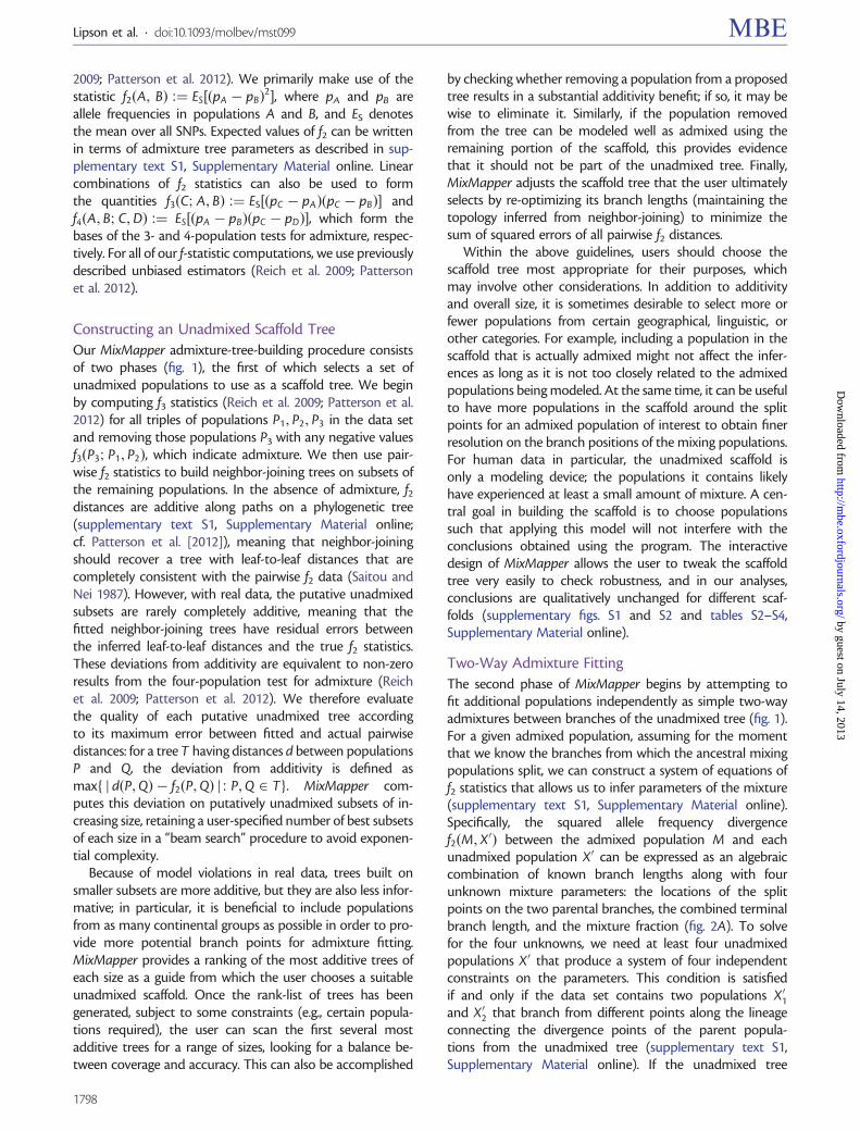
Our MixMapper admixture-tree-building procedure consistsof two phases (fig. 1), the first of which selects a set ofunadmixed populations to use as a scaffold tree. We beginby computing f3 statistics (Reich et al. 2009; Patterson et al.2012) for all triples of populations P1, P2, P3 in the data setand removing those populations P3 with any negative valuesf3ðP3; P1, P2Þ, which indicate admixture. We then use pair-wise f2 statistics to build neighbor-joining trees on subsets ofthe remaining populations. In the absence of admixture, f2distances are additive along paths on a phylogenetic tree(supplementary text S1, Supplementary Material online;cf. Patterson et al. [2012]), meaning that neighbor-joiningshould recover a tree with leaf-to-leaf distances that arecompletely consistent with the pairwise f2 data (Saitou andNei 1987). However, with real data, the putative unadmixedsubsets are rarely completely additive, meaning that thefitted neighbor-joining trees have residual errors betweenthe inferred leaf-to-leaf distances and the true f2 statistics.These deviations from additivity are equivalent to non-zeroresults from the four-population test for admixture (Reichet al. 2009; Patterson et al. 2012). We therefore evaluatethe quality of each putative unadmixed tree accordingto its maximum error between fitted and actual pairwisedistances: for a tree T having distances d between populationsP and Q, the deviation from additivity is defined asmaxf j dðP, QÞ � f2ðP, QÞ j : P, Q 2 Tg. MixMapper com-putes this deviation on putatively unadmixed subsets of in-creasing size, retaining a user-specified number of best subsetsof each size in a “beam search” procedure to avoid exponen-tial complexity.

Because of model violations in real data, trees built onsmaller subsets are more additive, but they are also less infor-mative; in particular, it is beneficial to include populationsfrom as many continental groups as possible in order to pro-vide more potential branch points for admixture fitting.MixMapper provides a ranking of the most additive trees ofeach size as a guide from which the user chooses a suitableunadmixed scaffold. Once the rank-list of trees has beengenerated, subject to some constraints (e.g., certain popula-tions required), the user can scan the first several mostadditive trees for a range of sizes, looking for a balance be-tween coverage and accuracy. This can also be accomplished

by checking whether removing a population from a proposedtree results in a substantial additivity benefit; if so, it may bewise to eliminate it. Similarly, if the population removedfrom the tree can be modeled well as admixed using theremaining portion of the scaffold, this provides evidencethat it should not be part of the unadmixed tree. Finally,MixMapper adjusts the scaffold tree that the user ultimatelyselects by re-optimizing its branch lengths (maintaining thetopology inferred from neighbor-joining) to minimize thesum of squared errors of all pairwise f2 distances.

Within the above guidelines, users should choose thescaffold tree most appropriate for their purposes, whichmay involve other considerations. In addition to additivityand overall size, it is sometimes desirable to select more orfewer populations from certain geographical, linguistic, orother categories. For example, including a population in thescaffold that is actually admixed might not affect the infer-ences as long as it is not too closely related to the admixedpopulations being modeled. At the same time, it can be usefulto have more populations in the scaffold around the splitpoints for an admixed population of interest to obtain finerresolution on the branch positions of the mixing populations.For human data in particular, the unadmixed scaffold isonly a modeling device; the populations it contains likelyhave experienced at least a small amount of mixture. A cen-tral goal in building the scaffold is to choose populationssuch that applying this model will not interfere with theconclusions obtained using the program. The interactivedesign of MixMapper allows the user to tweak the scaffoldtree very easily to check robustness, and in our analyses,conclusions are qualitatively unchanged for different scaf-folds (supplementary figs. S1 and S2 and tables S2–S4,Supplementary Material online).

Two-Way Admixture Fitting

The second phase of MixMapper begins by attempting tofit additional populations independently as simple two-wayadmixtures between branches of the unadmixed tree (fig. 1).For a given admixed population, assuming for the momentthat we know the branches from which the ancestral mixingpopulations split, we can construct a system of equations off2 statistics that allows us to infer parameters of the mixture(supplementary text S1, Supplementary Material online).Specifically, the squared allele frequency divergencef2ðM, X0Þ between the admixed population M and eachunadmixed population X0 can be expressed as an algebraiccombination of known branch lengths along with fourunknown mixture parameters: the locations of the splitpoints on the two parental branches, the combined terminalbranch length, and the mixture fraction (fig. 2A). To solvefor the four unknowns, we need at least four unadmixedpopulations X0 that produce a system of four independentconstraints on the parameters. This condition is satisfiedif and only if the data set contains two populations X01and X02 that branch from different points along the lineageconnecting the divergence points of the parent popula-tions from the unadmixed tree (supplementary text S1,Supplementary Material online). If the unadmixed tree

1798



Dow

nloaded from















contains n > 4 populations, we obtain a system of n equa-tions in the four unknowns that in theory is dependent. Inpractice, the equations are in fact slightly inconsistent becauseof noise in the f2 statistics and error in the point-admixturemodel, so we perform least-squares optimization to solve forthe unknowns; having more populations helps reduce theimpact of noise.

Algorithmically, MixMapper performs two-way admixturefitting by iteratively testing each pair of branches of theunadmixed tree as possible sources of the two ancestralmixing populations. For each choice of branches,MixMapper builds the implied system of equations andfinds the least-squares solution (under the constraints thatunknown branch lengths are nonnegative and the mixturefraction � is between 0 and 1), ultimately choosing the pairof branches and mixture parameters producing the smallestresidual norm. Our procedure for optimizing each system ofequations uses the observation that upon fixing �, thesystem becomes linear in the remaining three variables (sup-plementary text S1, Supplementary Material online). Thus,we can optimize the system by performing constrainedlinear least squares within a basic one-parameter optimiza-tion routine over � 2 ½0, 1�. To implement this approach,we applied MATLAB’s lsqlin and fminbnd functionswith a few auxiliary tricks to improve computational effi-ciency (detailed in the code).

Three-Way Admixture Fitting

MixMapper also fits three-way admixtures, that is, those forwhich one parent population is itself admixed (fig. 2B).Explicitly, after an admixed population M1 has been addedto the tree, MixMapper can fit an additional user-specifiedadmixed population M2 as a mixture between the M1 termi-nal branch and another (unknown) branch of the unadmixedtree. The fitting algorithm proceeds in a manner analogous tothe two-way mixture case: MixMapper iterates through eachpossible choice of the third branch, optimizing each impliedsystem of equations expressing f2 distances in terms ofmixture parameters. With two admixed populations, thereare now 2n + 1 equations, relating observed values off2ðM1, X0Þ and f2ðM2, X0Þ for all unadmixed populations X0,and also f2ðM1, M2Þ, to eight unknowns: two mixture frac-tions, �1 and �2, and six branch length parameters (fig. 2B).Fixing �1 and �2 results in a linear system as before, so weperform the optimization using MATLAB’s lsqlin withinfminsearch applied to �1 and �2 in tandem. The samemathematical framework could be extended to optimizingthe placement of populations with arbitrarily many ancestraladmixture events, but for simplicity and to reduce the riskof overfitting, we chose to limit this version of MixMapperto three-way admixtures.

Expressing Branch Lengths in Drift Units

All of the tree-fitting computations described thus far areperformed using pairwise distances in f2 units, which aremathematically convenient to work with owing to theiradditivity along a lineage (in the absence of admixture).However, f2 distances are not directly interpretable in the

same way as genetic drift D, which is a simple function oftime and population size:

D � 1� expð�t=2NeÞ � 2 � FST,

where t is the number of generations and Ne is the effectivepopulation size (Nei 1987). To convert f2 distances to driftunits, we apply a new formula, dividing twice the f2-length ofeach branch by the heterozygosity value that we infer for theancestral population at the top of the branch (supplementarytext S2, Supplementary Material online). Qualitatively speak-ing, this conversion corrects for the relative stretching of f2branches at different portions of the tree as a function ofheterozygosity (Patterson et al. 2012). To infer ancestral het-erozygosity values accurately, it is critical to use SNPs that areascertained in an outgroup to the populations involved,which we address later.

Before inferring heterozygosities at ancestral nodes of theunadmixed tree, we must first determine the location of theroot (which is neither specified by neighbor-joining norinvolved in the preceding analyses). MixMapper does so byiterating through branches of the unadmixed tree, temporar-ily rooting the tree along each branch, and then checking forconsistency of the resulting heterozygosity estimates.Explicitly, for each internal node P, we split its present-daydescendants (according to the re-rooted tree) into twogroups G1 and G2 according to which child branch of Pthey descend from. For each pair of descendants, one fromG1 and one from G2, we compute an inferred heterozygosityat P (supplementary text S2, Supplementary Material online).If the tree is rooted properly, these inferred heterozygositiesare consistent, but if not, there exist nodes P for which theheterozygosity estimates conflict. MixMapper thus infersthe location of the root as well as the ancestral heterozygosityat each internal node, after which it applies the drift lengthconversion as a postprocessing step on fitted f2 branchlengths.

Bootstrapping

To measure the statistical significance of our parameter esti-mates, we compute bootstrap confidence intervals (Efron1979; Efron and Tibshirani 1986) for the inferred branchlengths and mixture fractions. Our bootstrap procedure isdesigned to account for both the randomness of the driftprocess at each SNP and the random choice of individualssampled to represent each population. First, we divide thegenome into 50 evenly sized blocks, with the premise that thisscale should easily be larger than that of linkage disequilibriumamong our SNPs. Then, for each of 500 replicates, we resam-ple the data set by 1) selecting 50 of these SNP blocks atrandom with replacement; and 2) for each populationgroup, selecting a random set of individuals with replacement,preserving the number of individuals in the group.

For each replicate, we recalculate all pairwise f2 distancesand present-day heterozygosity values using the resampledSNPs and individuals (adjusting the bias-correction terms toaccount for the repetition of individuals) and then constructthe admixture tree of interest. Even though the mixtureparameters we estimate—branch lengths and mixture

1799



Dow

nloaded from










fractions—depend in complicated ways on many differentrandom variables, we can directly apply the nonparametricbootstrap to obtain confidence intervals (Efron andTibshirani 1986). For simplicity, we use a percentile bootstrap;thus, our 95% confidence intervals indicate 2.5 and 97.5 per-centiles of the distribution of each parameter among thereplicates.

Computationally, we parallelize MixMapper’s mixture-fit-ting over the bootstrap replicates using MATLAB’s ParallelComputing Toolbox.

Evaluating Fit Quality

When interpreting admixture inferences produced by meth-ods such as MixMapper, it is important to ensure that best-fitmodels are in fact accurate. Although formal tests for good-ness of fit do not generally exist for methods of this class,we use several criteria to evaluate the mixture fits producedby MixMapper and distinguish high-confidence results frompossible artifacts of overfitting or model violations.

First, we can compare MixMapper results to informationobtained from other methods, such as the 3-population test(Reich et al. 2009; Patterson et al. 2012). Negative f3 valuesindicate robustly that the tested population is admixed, andcomparing f3 statistics for different reference pairs can giveuseful clues about the ancestral mixing populations. Thus,while the three-population test relies on similar data toMixMapper, its simpler form makes it useful for confirmingthat MixMapper results are reasonable.

Second, the consistency of parameter values over boot-strap replicates gives an indication of the robustness of theadmixture fit in question. All results with real data havesome amount of associated uncertainty, which is a functionof sample sizes, SNP density, intrapopulation homogeneity,and other aspects of the data. Given these factors, we placeless faith in results with unexpectedly large error bars. Mostoften, this phenomenon is manifested in the placement ofancestral mixing populations: for poorly fitting admixtures,branch choices often change from one replicate to the next,signaling unreliable results.

Third, we find that results where one ancestral popula-tion is very closely related to the admixed population andcontributes more than 90% of the ancestry are often unreli-able. We expect that if we try to fit a nonadmixed popula-tion as an admixture, MixMapper should return a closelyrelated population as the first branch with mixture fraction� � 1 (and an arbitrary second branch). Indeed, we oftenobserve this pattern in the context of verifying that certainpopulations make sense to include in the scaffold tree.Further evidence of overfitting comes when the second an-cestry component, which contributes only a few percent,either bounces from branch to branch over the replicates,is located at the very tip of a leaf branch, or is historicallyimplausible.

Fourth, for any inferred admixture event, the two mixingpopulations must be contemporaneous. As we cannot re-solve the three pieces of terminal drift lengths leading toadmixed populations (fig. 2A) and our branch lengthsdepend both on population size and absolute time, we

cannot say for sure whether this property is satisfied forany given mixture fit. In some cases, however, it is clearthat no realization of the variables could possibly be consis-tent: for example, if we infer an admixture between a veryrecent branch and a very old one with a small value of thetotal mixed drift—and hence the terminal drift c—then wecan confidently say the mixture is unreasonable.

Finally, when available, we also use prior historical orother external knowledge to guide what we consider tobe reasonable. Sometimes, the model that appears to fitthe data best has implications that are clearly historicallyimplausible; often when this is true one or more of theevaluation criteria listed earlier can be invoked as well. Ofcourse, the most interesting findings are often those that arenew and surprising, but we subject such results to an extradegree of scrutiny.

Data Set and Ascertainment

We analyzed a SNP data set from 934 HGDP individualsgrouped in 53 populations (Rosenberg et al. 2002; Li et al.2008). Unlike most previous studies of the HGDP samples,however, we worked with recently published data generatedusing the new Affymetrix Axiom Human Origins Array(Patterson et al. 2012), which was designed with a simpleascertainment scheme for accurate population genetic infer-ence (Keinan et al. 2007). It is well known that ascertain-ment bias can cause errors in estimated divergences amongpopulations (Clark et al. 2005; Albrechtsen et al. 2010), aschoosing SNPs based on their properties in modern popu-lations induces nonneutral spectra in related samples.Although there do exist methods to correct for ascertain-ment bias (Nielsen et al. 2004), it is much more desirableto work with a priori bias-free data, especially given thattypical SNP arrays are designed using opaque ascertainmentschemes.

To avoid these pitfalls, we used panel 4 of the new array,which consists of 163,313 SNPs that were ascertained asheterozygous in the genome of a San individual (Keinanet al. 2007). This panel is special because there is evidencethat the San are approximately an outgroup to all othermodern-day human populations (Li et al. 2008; Gronauet al. 2011). Thus, while the panel 4 ascertainment schemedistorts the San allele frequency spectrum, it is nearly neutralwith respect to all other populations. In other words, we canthink of the ascertainment as effectively choosing a set ofSNPs (biased toward San heterozygosity) at the commonancestor of the remaining 52 populations, after which driftoccurs in a bias-free manner. We excluded 61,369 SNPs thatare annotated as falling between the transcription start siteand end site of a gene in the UCSC Genome Browser data-base (Fujita et al. 2011). Most of the excluded SNPs are notwithin actual exons, but as expected, the frequency spectraat these “gene region” loci were slightly shifted toward fixedclasses relative to other SNPs, indicative of the action ofselection (supplementary fig. S5, Supplementary Materialonline). As we assume neutrality in all of our analyses, wechose to remove these SNPs.

1800



Dow

nloaded from




Simulations

Our first simulated tree was generated using the ms (Hudson2002) command

ms 350 500 -t 50 -r 99.9998 500000 -I 7 50 5050 50 50 50 50 -n 7 2-n 12-n 22-ej 0.04 21-es0.02 6 0.4 -ej 0.06 6 3 -ej 0.04 8 5 -ej 0.08 5 4-ej 0.12 4 3 -ej 0.2 3 1 -ej 0.3 1 7 -en 0.3 7 1.

After ascertainment, we used a total of 95,997 SNPs.Our second simulated tree was generated with the

command

ms 550 500 -t 50 -r 99.9998 500000 -I 11 50 5050 50 50 50 50 50 50 50 50 -n 11 2 -n 1 2 -n 2 2-em 0.002 4 3 253.8 -em 0.004 4 3 0 -es 0.0028 0.2 -en 0.002 8 2 -ej 0.02 8 2 -ej 0.02 4 5-ej 0.04 2 1 -ej 0.04 5 3 -es 0.04 12 0.4 -es0.04 9 0.2 -em 0.042 10 9 253.8 -em 0.044 10 90 -ej 0.06 12 7 -ej 0.06 9 7 -ej 0.06 14 10 -ej0.06 13 10 -ej 0.08 7 6 -ej 0.12 6 3 -ej 0.1610 3 -ej 0.2 3 1 -ej 0.3 1 11 -en 0.3 11 1.

After ascertainment, we used a total of 96,258 SNPs. Whenanalyzing this data set in TreeMix, we chose to fit a total offive admixtures based on the residuals of the pairwisedistances (maximum of approximately three standarderrors) and our knowledge that this is the number in thetrue admixture tree (to make for a fair comparison).

Software

Source code for the MixMapper software is available at http://groups.csail.mit.edu/cb/mixmapper/ (last accessed June 14,2013).

Supplementary MaterialSupplementary figures S1–S5, tables S1–S5, and text S1 andS2 are available at Molecular Biology and Evolution online(http://www.mbe.oxfordjournals.org/).

Acknowledgments

The authors thank George Tucker and Joe Pickrell for helpfuldiscussions and the reviewers and editors for numeroussuggestions that improved the manuscript. This work wassupported by the National Science Foundation GraduateResearch Fellowship to M.L., P.L., and A.L.; HOMINID grant1032255 to D.R. and N.P.; and the National Institutes of Healthgrant GM100233 to D.R. and N.P.

ReferencesAlbrechtsen A, Nielsen F, Nielsen R. 2010. Ascertainment biases in SNP

chips affect measures of population divergence. Mol Biol Evol. 27:2534–2547.

Bramanti B, Thomas M, Haak W, et al. (11 co-authors). 2009. Geneticdiscontinuity between local hunter-gatherers and Central Europe’sfirst farmers. Science 326:137–140.

Cavalli-Sforza L, Edwards A. 1967. Phylogenetic analysis: models andestimation procedures. Am J Hum Genet. 19:233–257.

Chikhi L, Bruford M, Beaumont M. 2001. Estimation of admixture pro-portions: a likelihood-based approach using Markov chain MonteCarlo. Genetics 158:1347–1362.

Clark A, Hubisz M, Bustamante C, Williamson S, Nielsen R. 2005.Ascertainment bias in studies of human genome-wide polymor-phism. Genome Res. 15:1496–1502.

Der Sarkissian C, Balanovsky O, Brandt G, et al. (11 co-authors). 2013.Ancient DNA reveals prehistoric gene-flow from Siberia in thecomplex human population history of North East Europe. PLoSGenet. 9:e1003296.

Dupanloup I, Bertorelle G, Chikhi L, Barbujani G. 2004. Estimatingthe impact of prehistoric admixture on the genome of Europeans.Mol Biol Evol. 21:1361–1372.

Efron B. 1979. Bootstrap methods: another look at the jackknife.Ann Stat. 7:1–26.

Efron B, Tibshirani R. 1986. Bootstrap methods for standard errors,confidence intervals, and other measures of statistical accuracy.Stat Sci. 1:54–75.

Fujita P, Rhead B, Zweig A, et al. (11 co-authors). 2011. The UCSCGenome Browser database: update 2011. Nucleic Acids Res. 39:D876–D882.

Gravel S, Henn B, Gutenkunst R, et al. (11 co-authors). 2011.Demographic history and rare allele sharing among human popu-lations. Proc Natl Acad Sci U S A. 108:11983–11988.

Green R, Krause J, Briggs A, et al. (11 co-authors). 2010. A draft sequenceof the Neandertal genome. Science 328:710–722.

Gronau I, Hubisz M, Gulko B, Danko C, Siepel A. 2011. Bayesian inferenceof ancient human demography from individual genome sequences.Nat Genet. 43:1031–1034.

Haak W, Balanovsky O, Sanchez J, et al. (11 co-authors). 2010. AncientDNA from European early Neolithic farmers reveals their NearEastern affinities. PLoS Biol. 8:e1000536.

Hudson RR. 2002. Generating samples under a Wright–Fisher neutralmodel of genetic variation. Bioinformatics 18:337–338.

HUGO Pan-Asian SNP Consortium. 2009. Mapping human geneticdiversity in Asia. Science 326:1541–1545.

Huson D, Bryant D. 2006. Application of phylogenetic networks inevolutionary studies. Mol Biol Evol. 23:254–267.

Keinan A, Mullikin J, Patterson N, Reich D. 2007. Measurement of thehuman allele frequency spectrum demonstrates greater genetic driftin East Asians than in Europeans. Nat Genet. 39:1251–1255.

Keller A, Graefen A, Ball M, et al. (11 co-authors). 2012. New insights intothe Tyrolean Iceman’s origin and phenotype as inferred by whole-genome sequencing. Nat Commun. 3:698.

Laval G, Patin E, Barreiro L, Quintana-Murci L. 2010. Formulating ahistorical and demographic model of recent human evolutionbased on resequencing data from noncoding regions. PLoS One 5:e10284.

Li J, Absher D, Tang H, et al. (11 co-authors). 2008. Worldwide humanrelationships inferred from genome-wide patterns of variation.Science 319:1100–1104.

Loh PR, Lipson M, Patterson N, Moorjani P, Pickrell JK, Reich D, Berger B.2013. Inferring admixture histories of human populations using link-age disequilibrium. Genetics 193:1233–1254.

Nei M. 1987. Molecular evolutionary genetics. New York: ColumbiaUniversity Press.

Nielsen R, Hubisz M, Clark A. 2004. Reconstituting the frequency spec-trum of ascertained single-nucleotide polymorphism data. Genetics168:2373–2382.

Patterson N, Moorjani P, Luo Y, Mallick S, Rohland N, Zhan Y,Genschoreck T, Webster T, Reich D. 2012. Ancient admixture inhuman history. Genetics 192:1065–1093.

Pickrell J, Pritchard J. 2012. Inference of population splits and mix-tures from genome-wide allele frequency data. PLoS Genet. 8:e1002967.

Pinhasi R, Thomas M, Hofreiter M, Currat M, Burger J. 2012. The genetichistory of Europeans. Trends Genet. 28:496–505.

Pool J, Hellmann I, Jensen J, Nielsen R. 2010. Population genetic inferencefrom genomic sequence variation. Genome Res. 20:291–300.

Reich D, Green R, Kircher M, et al. (11 co-authors). 2010. Genetic historyof an archaic hominin group from Denisova Cave in Siberia. Nature468:1053–1060.

Reich D, Patterson N, Kircher M, et al. (11 co-authors). 2011. Denisovaadmixture and the first modern human dispersals into SoutheastAsia and Oceania. Am J Hum Genet. 89:516–528.

1801



Dow

nloaded from

http://groups.csail.mit.edu/cb/mixmapper/

http://groups.csail.mit.edu/cb/mixmapper/





http://www.mbe.oxfordjournals.org/


Reich D, Thangaraj K, Patterson N, Price A, Singh L. 2009. ReconstructingIndian population history. Nature 461:489–494.

Rosenberg N, Pritchard J, Weber J, Cann H, Kidd K, Zhivotovsky L,Feldman M. 2002. Genetic structure of human populations.Science 298:2381–2385.

Saitou N, Nei M. 1987. The neighbor-joining method: a newmethod for reconstructing phylogenetic trees. Mol Biol Evol. 4:406–425.

Semino O, Passarino G, Oefner P, et al. (11 co-authors). 2000. Thegenetic legacy of Paleolithic Homo sapiens sapiens in extantEuropeans: a Y chromosome perspective. Science 290:1155–1159.

Siren J, Marttinen P, Corander J. 2011. Reconstructing population histo-ries from single nucleotide polymorphism data. Mol Biol Evol. 28:673–683.

Skoglund P, Malmstrom H, Raghavan M, Stora J, Hall P, Willerslev E,Gilbert M, Gotherstrom A, Jakobsson M. 2012. Origins and geneticlegacy of Neolithic farmers and hunter-gatherers in Europe. Science336:466–469.

Soares P, Achilli A, Semino O, Davies W, Macaulay V, Bandelt H, TorroniA, Richards M. 2010. The archaeogenetics of Europe. Curr Biol. 20:R174–R183.

Sousa V, Fritz M, Beaumont M, Chikhi L. 2009. Approximate Bayesiancomputation without summary statistics: the case of admixture.Genetics 181:1507–1519.

Wall J, Lohmueller K, Plagnol V. 2009. Detecting ancient admixtureand estimating demographic parameters in multiple humanpopulations. Mol Biol Evol. 26:1823–1827.

Wang J. 2003. Maximum-likelihood estimation of admixture propor-tions from genetic data. Genetics 164:747–765.

Xu S, Pugach I, Stoneking M, et al. (6 co-authors). 2012. Genetic datingindicates that the Asian–Papuan admixture through easternIndonesia corresponds to the Austronesian expansion. Proc NatlAcad Sci U S A. 109:4574–4579.

Yu Y, Degnan J, Nakhleh L. 2012. The probability of a gene tree topologywithin a phylogenetic network with applications to hybridizationdetection. PLoS Genet. 8:e1002660.

1802



Dow

nloaded from


Efficient Moment-Based Inference of Admixture Parameters

Documents

Transcript of Efficient Moment-Based Inference of Admixture Parameters