Efficient Methods for Automatic Speech Recognition

Alexander Seward

Doctoral Dissertation Royal Institute of Technology

Stockholm 2003

Akademisk avhandling som med tillstånd av Kungliga Tekniska Högskolan framlägges till offentlig granskning för avläggande av teknologie doktorsexamen onsdagen den 17 december 2003 kl. 10.00 i Kollegiesalen, Kungliga Tekniska Högskolan, Valhallavägen 79, Stockholm. ISBN 91-7283-657-1 TRITA-TMH 2003:14 ISSN 1104-5787 © Alexander Seward, November 2003. Universitetsservice US AB, Stockholm 2003.

Abstract

This thesis presents work in the area of automatic speech recognition (ASR). The thesis focuses on methods for increasing the efficiency of speech recognition systems and on techniques for efficient representation of different types of knowledge in the decoding process. In this work, several decoding algorithms and recognition systems have been developed, aimed at various recognition tasks.

The thesis presents the KTH large vocabulary speech recognition system. The system was developed for online (live) recognition with large vocabularies and complex language models. The system utilizes weighted transducer theory for efficient representation of different knowledge sources, with the purpose of optimizing the recognition process.

A search algorithm for efficient processing of hidden Markov models (HMMs) is presented. The algorithm is an alternative to the classical Viterbi algorithm for fast computation of shortest paths in HMMs. It is part of a larger decoding strategy aimed at reducing the overall computational complexity in ASR. In this approach, all HMM computations are completely decoupled from the rest of the decoding process. This enables the use of larger vocabularies and more complex language models without an increase of HMM-related computations.

Ace is another speech recognition system developed within this work. It is a platform aimed at facilitating the development of speech recognizers and new decoding methods.

A real-time system for low-latency online speech transcription is also presented. The system was developed within a project with the goal of improving the possibilities for hard-of-hearing people to use conventional telephony by providing speech-synchronized multimodal feedback. This work addresses several additional requirements implied by this special recognition task.

Acknowledgements First of all, I would like to acknowledge my advisors Rolf Carlson and Björn Granström for supporting this work and for giving me the opportunity to pursue my research interests and ideas. Also, I am grateful to my assistant advisors Kjell Elenius and Mats Blomberg for all the excellent feedback they have provided. Special thanks to Kåre Sjölander who always been very helpful and with whom I have had many fruitful discussions. Many thanks to Becky Hincks, David House and Peta Sjölander for all proofreading work. Last but not least, I would like acknowledge all my colleagues at the department without whom this work would have been a lot harder. AT&T Labs Research should also be acknowledged for providing special FSM related software to KTH. This research has been funded by Vattenfall and was carried out at the Centre for Speech Technology at KTH, supported by VINNOVA (the Swedish Agency for Innovation Systems), KTH and participating partners.

Alec Seward, November 2003

Contents 1 Included papers ...............................................................................................................................3 2 Introduction.....................................................................................................................................5 3 Hidden Markov Models ................................................................................................................10 4 The decoding problem ..................................................................................................................12

4.1 Determining the optimal HMM state sequence ...................................................................14 5 Weighted finite-state transducers..................................................................................................17

5.1 Definitions...........................................................................................................................17 5.2 WFSTs and the recognition cascade....................................................................................22 5.3 Weighted FST operations ....................................................................................................24

6 Language modeling.......................................................................................................................26 6.1 Context-free grammars and regular grammars ....................................................................26 6.2 Markovian grammars (n-gram) ...........................................................................................27

7 Context dependency......................................................................................................................28 7.1 Search in different contexts .................................................................................................30

8 Summary of papers .......................................................................................................................32 8.1 Paper 1. The KTH Large Vocabulary Continuous Speech Recognition System.................33 8.2 Paper 2. A Fast HMM Match Algorithm for Very Large Vocabulary Speech Recognition34 8.3 Paper 3. Low-Latency Incremental Speech Transcription in the Synface Project...............36 8.4 Paper 4. Transducer optimizations for tight-coupled decoding. ..........................................38 8.5 Paper 5. A tree-trellis N-best decoder for stochastic context-free grammars ......................39

9 References.....................................................................................................................................40 10 Appendix..................................................................................................................................44

10.1 Composition ........................................................................................................................44 10.2 Concatenation......................................................................................................................47 10.3 Connection ..........................................................................................................................49 10.4 Determinization ...................................................................................................................50 10.5 Difference............................................................................................................................51 10.6 Epsilon removal...................................................................................................................53 10.7 Intersection ..........................................................................................................................54 10.8 Inversion..............................................................................................................................56 10.9 Kleene closure .....................................................................................................................57 10.10 Minimization ..................................................................................................................58 10.11 Projection........................................................................................................................59 10.12 Pruning ...........................................................................................................................60 10.13 Reversal ..........................................................................................................................61 10.14 Shortest path ...................................................................................................................62 10.15 Union (sum)....................................................................................................................63 10.16 Weight pushing...............................................................................................................65

1

2

1 Included papers Paper 1. Seward, A., The KTH Large Vocabulary Continuous Speech

Recognition System, TMH-QPSR (to appear), KTH, Stockholm, Sweden, 2004.

Paper 2. Seward, A., A Fast HMM Match Algorithm for Very Large

Vocabulary Speech Recognition, Journal of Speech Communication, doi:10.1016/j.specom.2003.08.005, 2003.

Paper 3. Seward, A., Low-Latency Incremental Speech Transcription

in the Synface Project, Proceedings of the European Conference on Speech Communication and Technology (Eurospeech), vol 2, pp 1141-1144, Geneva, Switzerland, 2003.

Paper 4. Seward, A., Transducer Optimizations for Tight-Coupled

Decoding, Proceedings of the European Conference on Speech Communication and Technology (Eurospeech), vol 3, pp 1607-1610, Aalborg, Denmark, 2001.

Paper 5. Seward, A., A Tree-Trellis N-best Decoder for Stochastic

Context-Free Grammars, Proceedings of the International Conference on Spoken Language Processing, vol 4, pp 282-285, Beijing, China, 2000.

3

4

2 Introduction Long before advanced computers made their entrance into our world, humans have envisioned being able to communicate with machines in our most natural way – by spoken language. For more than half a century, research has been conducted in the field of automatic speech recognition (ASR), which constitutes an important part in the fulfillment of this vision. Despite the considerable amount of research resources invested in this task, many questions still remain to be answered. This is because the problem is very complex and requires solutions from several disciplines. However, achievements within the fields of pattern matching, signal processing, phonetics, natural language processing, computer science, information theory and artificial intelligence, along with the progression of computer technology, have taken us several steps closer to the goal.

Early attempts at ASR were based on template matching techniques. Template matching means that the incoming speech signal is compared to a set of reference patterns, or templates. By having a template for each word that the recognizer should be able to handle, recognition of isolated words is possible. This principle was extended to recognition of connected words from a limited vocabulary, e.g. connected digits. These simple types of pattern matchers have several limitations that make them inadequate for speaker-independent recognition of continuous speech with large vocabularies. The approach with whole-word models inherently implies a practical limitation since it complicates the addition of new words to the recognizer vocabulary. Handling pronunciation variation is equally problematic. For these reasons, the concept of whole-word models has been replaced by subword phonetic units in contemporary speech recognition systems. In general, these consist of phone models, which when made context-sensitive are called n-phone models. This set of smaller units, which make up an acoustic model (AM), can be concatenated to model whole words. The approach enables the use of pronunciation dictionaries which improves the flexibility of adding new words and pronunciations to the vocabulary. Moreover, in continuous speech there is no silence or other acoustic event associated with word boundaries. These challenges have paved the way

5

for flexible pattern matching devices, such as hidden Markov models (HMMs), which are probabilistic classifiers that can be generated from collected speech data. HMMs are discussed in more detail in Chapter 3. In information theory, Shannon surveyed aspects of Markov sources (Shannon 1948). The basic HMM theory was published by Baum and his colleagues in a series of papers (Baum and Petrie 1966, Baum and Eagon 1967). HMMs were first applied in automatic speech recognition in the mid seventies (Baker 1975, Jelinek 1976).

HMMs are suitable for acoustic modeling in a context of concatenated acoustic-phonetic units. Although there are deficiencies associated with these devices for acoustic modeling, they have proven effective for the processing of continuous speech. HMMs have a relatively good ability to handle variation in speaking rate and local temporal phenomena. Moreover, pronunciation variation of words using subword HMMs is handled by the help of a pronunciation dictionary. Phonetic coarticulation can also be handled by augmenting HMMs with context-dependency modeling (Schwartz et al. 1985, Lee 1990). Phonetic context-dependency can also be applied across word boundaries (Alleva et al. 1992, Woodland et al. 1994, Beyerlein et al. 1997). In addition to these factors, the evolution of more efficient algorithms and the ability to apply different acoustic match components have contributed to the applicability of HMMs in automatic speech recognition.

However, acoustic-phonetic pattern matchers are not sufficient to solve the problem of ASR. It is important to understand that the information is only partially in the acoustic signal. It is only with the help of the listener’s composed knowledge, on several levels, that the information can be made complete and be understood. The same process must be undertaken by an artificial listener in the form of a computer. Whereas for us humans it is a hidden process on a subconscious level, it must in the artificial case be approached explicitly.

In state-of-the-art ASR systems, this is done in the decoding process, which is characterized by knowledge sources (KS) on different levels that together contribute information to hypothesize what has been said. The decoding process can be described in terms of a cascade of applied knowledge sources (Jelinek 1976). The acoustic level involves preprocessing of the speech signal, extraction of parametric features and

6

acoustic matching. Higher-level knowledge sources, representing phonetic, lexical and syntactical knowledge, are also incorporated (Figure 1). The inclusion of semantic and pragmatic knowledge, which is crucial in the understanding process, may also be useful in the decoding process.

Figure 1. Simplified speech recognition cascade

Some early attempts at incorporating higher-level knowledge in ASR systems were based on the use of expert knowledge within different areas of speech processing, ranging from spectrogram reading and formant patterns, to syntactical knowledge about the language obtained from linguists. Expert systems have had limited success, mainly because a formalization of expert knowledge in a computer generally implies manual rule based methods that are less suited for modeling the characteristics of spoken language. For the purpose of handling the high irregularity and variance that characterize spoken language, there has been a trend towards the application of data driven methods for information extraction. These methods are based on the creation of statistical models, such as Markov models, or statistically generated rules, for representing knowledge sources. Statistical models are created from large amounts of data by an artificial learning process commonly referred to as training. This process involves collection of a large data set: the training material. By the application of training algorithms, models are produced at different levels, with the purpose of modeling the training material as accurately as possible and thereby the specific aspects of spoken language. Data driven methods are typically also applied for the creation of language models (LMs) with the purpose of modeling the syntactical, or grammatical, aspects of the language. In the decoder, language models are represented by grammars, which are produced from corpora in a process referred to as language model training. In Chapter 6, we give an overview of two classes of grammars used in ASR: context-free grammars and Markovian grammars (n-grams). Using Markovian

Feature extraction

Acoustic match

Lexical knowledge

Syntactical knowledge

7

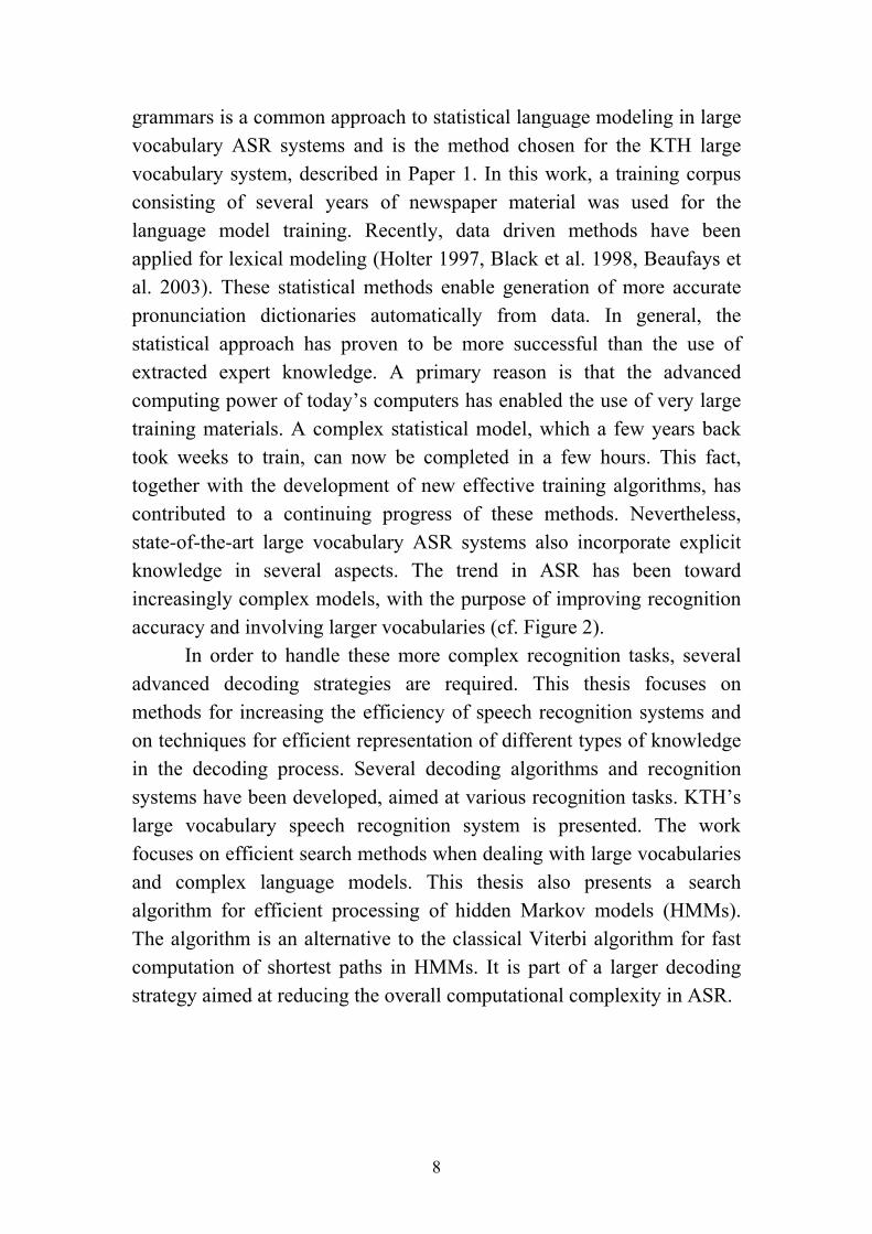
grammars is a common approach to statistical language modeling in large vocabulary ASR systems and is the method chosen for the KTH large vocabulary system, described in Paper 1. In this work, a training corpus consisting of several years of newspaper material was used for the language model training. Recently, data driven methods have been applied for lexical modeling (Holter 1997, Black et al. 1998, Beaufays et al. 2003). These statistical methods enable generation of more accurate pronunciation dictionaries automatically from data. In general, the statistical approach has proven to be more successful than the use of extracted expert knowledge. A primary reason is that the advanced computing power of today’s computers has enabled the use of very large training materials. A complex statistical model, which a few years back took weeks to train, can now be completed in a few hours. This fact, together with the development of new effective training algorithms, has contributed to a continuing progress of these methods. Nevertheless, state-of-the-art large vocabulary ASR systems also incorporate explicit knowledge in several aspects. The trend in ASR has been toward increasingly complex models, with the purpose of improving recognition accuracy and involving larger vocabularies (cf. Figure 2).

In order to handle these more complex recognition tasks, several advanced decoding strategies are required. This thesis focuses on methods for increasing the efficiency of speech recognition systems and on techniques for efficient representation of different types of knowledge in the decoding process. Several decoding algorithms and recognition systems have been developed, aimed at various recognition tasks. KTH’s large vocabulary speech recognition system is presented. The work focuses on efficient search methods when dealing with large vocabularies and complex language models. This thesis also presents a search algorithm for efficient processing of hidden Markov models (HMMs). The algorithm is an alternative to the classical Viterbi algorithm for fast computation of shortest paths in HMMs. It is part of a larger decoding strategy aimed at reducing the overall computational complexity in ASR.

8

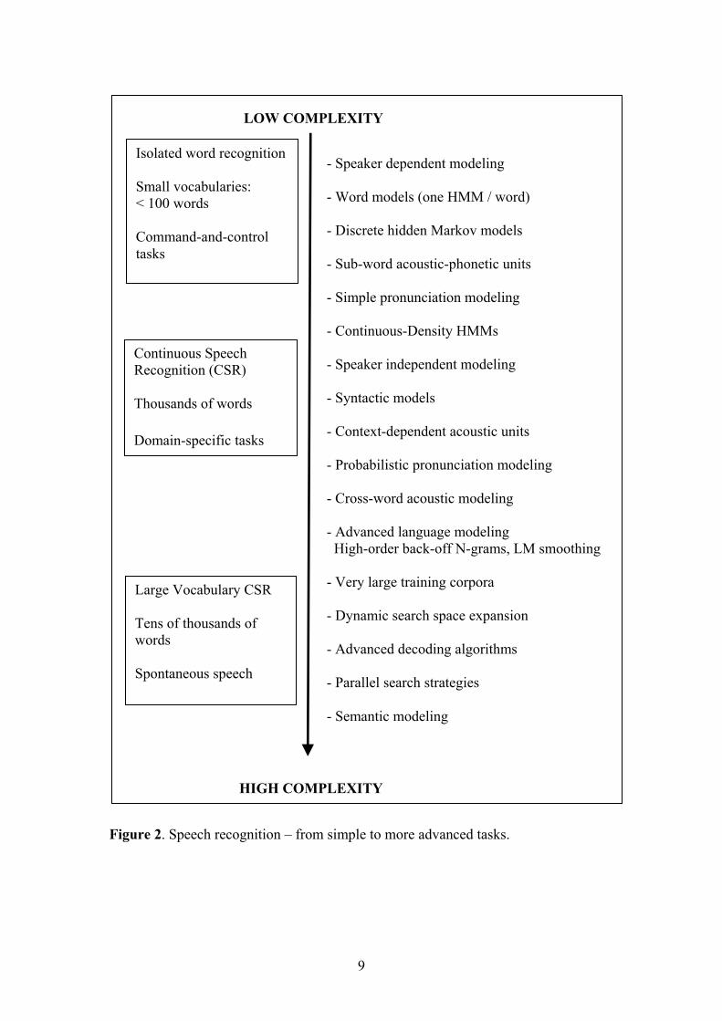
LOW COMPLEXITY

Isolated word recognition - Speaker dependent modeling Small vocabularies: - Word models (one HMM / word) < 100 words - Discrete hidden Markov models Command-and-control

tasks - Sub-word acoustic-phonetic units - Simple pronunciation modeling - Continuous-Density HMMs Continuous Speech

Recognition (CSR) - Speaker independent modeling - Syntactic models Thousands of words - Context-dependent acoustic units Domain-specific tasks - Probabilistic pronunciation modeling - Cross-word acoustic modeling - Advanced language modeling High-order back-off N-grams, LM smoothing - Very large training corpora Large Vocabulary CSR - Dynamic search space expansion Tens of thousands of

words - Advanced decoding algorithms Spontaneous speech - Parallel search strategies - Semantic modeling

HIGH COMPLEXITY

Figure 2. Speech recognition – from simple to more advanced tasks.

9

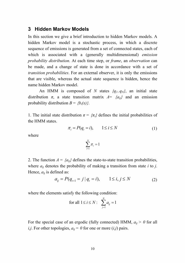
3 Hidden Markov Models In this section we give a brief introduction to hidden Markov models. A hidden Markov model is a stochastic process, in which a discrete sequence of emissions is generated from a set of connected states, each of which is associated with a (generally multidimensional) emission probability distribution. At each time step, or frame, an observation can be made, and a change of state is done in accordance with a set of transition probabilities. For an external observer, it is only the emissions that are visible, whereas the actual state sequence is hidden, hence the name hidden Markov model.

An HMM is composed of N states q1..qN, an initial state distribution π, a state transition matrix A= aij and an emission probability distribution B = bi(x). 1. The initial state distribution π = πi defines the initial probabilities of the HMM states.

( ), 1i tP q i i Nπ = = ≤ ≤ (1) where

1

1N

iiπ

=

=∑

2. The function A = aij defines the state-to-state transition probabilities, where aij denotes the probability of making a transition from state i to j. Hence, aij is defined as:

(2) 1( | ), 1 ,ij t ta P q j q i i j N+= = = ≤ ≤

where the elements satisfy the following condition:

1

for all 1 : 1N

ijj

i N a=

≤ ≤ =∑

For the special case of an ergodic (fully connected) HMM, aij > 0 for all i,j. For other topologies, aij = 0 for one or more (i,j) pairs.

10

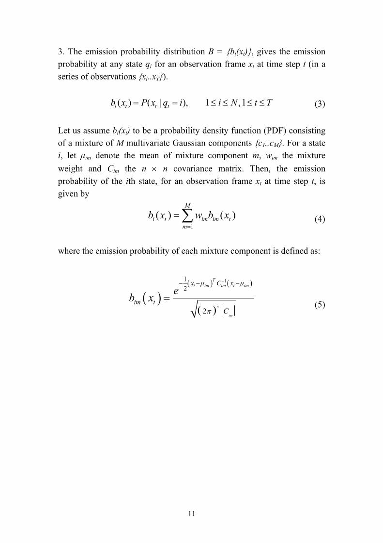
3. The emission probability distribution B = bi(xt), gives the emission probability at any state qi for an observation frame xt at time step t (in a series of observations xi..xT). (3) ( ) ( | ), 1 ,1i t t tb x P x q i i N t T= = ≤ ≤ ≤ ≤

Let us assume bi(xt) to be a probability density function (PDF) consisting of a mixture of M multivariate Gaussian components c1..cM. For a state i, let µim denote the mean of mixture component m, wim the mixture weight and Cim the n × n covariance matrix. Then, the emission probability of the ith state, for an observation frame xt at time step t, is given by

(4) 1

( ) ( )M

i t im im tm

b x w b x=

=∑ where the emission probability of each mixture component is defined as:

( )( ) (

( )

)112

2n

im

Tt im im t imx C x

im tC

eb xµ µ

π

−− − −

= (5)

11

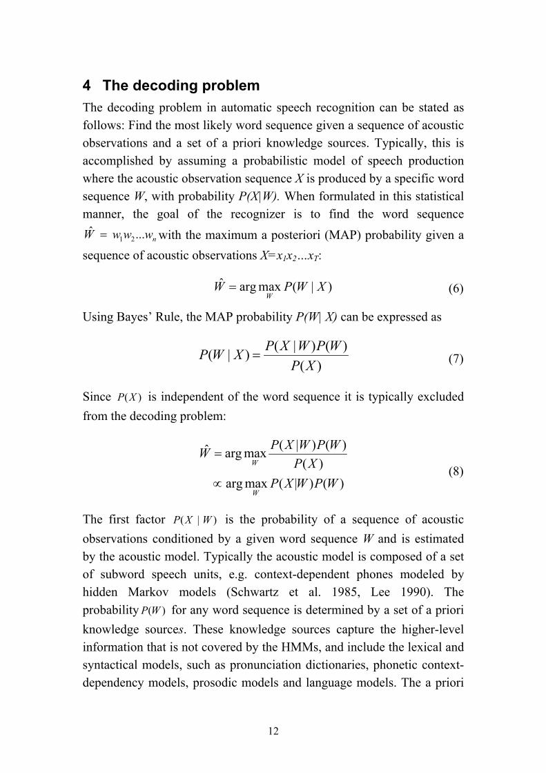
4 The decoding problem The decoding problem in automatic speech recognition can be stated as follows: Find the most likely word sequence given a sequence of acoustic observations and a set of a priori knowledge sources. Typically, this is accomplished by assuming a probabilistic model of speech production where the acoustic observation sequence X is produced by a specific word sequence W, with probability P(X|W). When formulated in this statistical manner, the goal of the recognizer is to find the word sequence

with the maximum a posteriori (MAP) probability given a sequence of acoustic observations X=x1x2…xT:

nwwwW ...ˆ21=

(6) ˆ arg max ( | )W

W P W= X

Using Bayes’ Rule, the MAP probability P(W| X) can be expressed as

( | ) ( )( | )

( )P X W P WP W X

P X= (7)

Since is independent of the word sequence it is typically excluded from the decoding problem:

)(XP

( | ) ( )ˆ arg max( )

arg max ( | ) ( )

W

W

P X W P WWP X

P X W P W

=

∝ (8)

The first factor is the probability of a sequence of acoustic observations conditioned by a given word sequence W and is estimated by the acoustic model. Typically the acoustic model is composed of a set of subword speech units, e.g. context-dependent phones modeled by hidden Markov models (Schwartz et al. 1985, Lee 1990). The probability for any word sequence is determined by a set of a priori knowledge sources. These knowledge sources capture the higher-level information that is not covered by the HMMs, and include the lexical and syntactical models, such as pronunciation dictionaries, phonetic context-dependency models, prosodic models and language models. The a priori

)|( WXP

)(WP

12

models define a probabilistic mapping, so that any word sequence W can be translated to at least one sequence of subword HMMs Λw.

Hence, the decoding problem can be equivalently formulated in terms of finding the HMM sequence with the MAP probability:

)...λλ(λΛ nw 21=ˆ

ˆ arg maxw

w wΛ wΛ P(X|Λ )P(Λ )= (9)

where Λw maps to a word sequence W with an a priori probability P(Λw)=P(W). By summation over all possible state sequences Q ,the decoding problem can be formulated as:

(10) w

ˆ arg max

Since X is conditionally independent of Λ ,given Qˆ arg max

w

w

w w wΛ Q

w w wΛ Q

Λ P(X |Q,Λ )P(Q | Λ )P(Λ )

Λ P(Λ ) P(Q | Λ )P(X |Q)

=

=

∑

∑

w

The Forward algorithm (Rabiner and Juang 1993, Jelinek 1998), is an algorithm for computing emission probabilities by summation over state sequences. Typically, the decoding problem is simplified by employing the Viterbi approximation, which implies the adoption of a shortest-path optimality criterion. This means that the sum of all paths is approximated by the optimal, or shortest path, i.e. the state sequence of highest likelihood. Accordingly, the MAP recognition criterion is approximated to:

(11)

ˆ arg max max

arg max maxw

w w

w w wΛ Q

wΛ Q Q

Λ P(Λ ) P(Q | Λ )P(X |Q)

P(Λ ) P(Q)P(X |Q)∈

≅

=

13

where Qw is the set of state sequences Q= (q1q2…qT) that corresponds to the HMM sequence Λw: Q:P(Q , Λw)>0. Hence, the decoding problem is solved by a search for the HMM state sequence of highest likelihood according to the acoustic model and the a priori knowledge sources.

4.1 Determining the optimal HMM state sequence The concept of Dynamic Programming (DP) (Bellman 1957, Silverman and Morgan 1990) has proven very efficient for finding the optimal state sequence in HMMs, given a series of observations. Dynamic programming denotes a class of algorithmic techniques in which optimization problems are solved by caching subproblem solutions rather than recomputing them. The Viterbi algorithm (Viterbi 1967, Forney 1973) is a DP method for computation of the optimal state paths of HMMs given a sequence of observations. The Viterbi algorithm is based on the DP principles behind Dijkstra’s algorithm (Dijkstra 1959) for finding the shortest paths in positively weighted graphs. Shortest paths problems are also covered by other classic papers (Ford and Fulkerson 1956, Bellman 1958, Warshall 1962).

The underlying DP principle of Dijkstra’s algorithm is simple. Assume that we want to find the shortest path from a point A to a point B. If we can determine an intermediate point C on this shortest path, the problem can be divided into two separate smaller problems of finding the shortest path from A to C, and from C to B. These two smaller problems can be divided even further if we can find intermediate points on these shorter paths. Hence, this suggests a recursive solution, where the problem is solved in smaller parts by DP.

Dijkstra’s algorithm finds the single-source shortest paths in graphs with positively weighted edges, i.e. the shortest paths from a vertex to all other vertices. The algorithm starts from a vertex x to find the shortest paths to all other vertices. At each iteration, it identifies a new vertex v, for which the shortest path from x to v is known. The algorithm then maintains a set of vertices to which it currently knows the shortest path from x, and this set grows by one vertex each iteration.

An HMM, in the context of shortest paths, can be regarded as a weighted graph, with probabilistic transitions instead of the weighted edges and states instead of vertices. In addition, there is a positive cost

14

associated with each HMM state that varies over time and is determined by the incoming observations. In this sense, the principle of Dijkstra’s algorithm is applicable, as there are only positive costs associated with transitions or states.

The Viterbi algorithm enables computation of the optimal state sequence Q for an HMM λ=π,A,B together with the associated MAP probability P(Q,X| λ). The likelihood of the optimal state sequence given a sequence of the observations X=(x1x2…xT) is calculated by defining a variable )(itδ as the best score at time t which accounts for the first t observations along the optimal path that ends in state i:

(12) 1 2 1

1 2 1 1 2max )t

t t tq q ...,qδ (i) P(q q ...q ,q i,x x ...x | λ

−−= = t

≤ ≤

The optimal path likelihood is then inductively retrievable by the Viterbi algorithm as:

(13) ( )

1 1

11

e

1. Initialization:, 1

2. Recursion:

2 1max

3. Termination:max Q is the set of finalstates of λ

i e

i i

t t ij j ti N

Ti:q Q

δ (i) π b (x ) i N

δ (j) δ (i)a b (x ), t T, j N

P* δ (i),

−≤ ≤

∀ ∈

= ≤ ≤

= ≤ ≤

=

15

State

Time

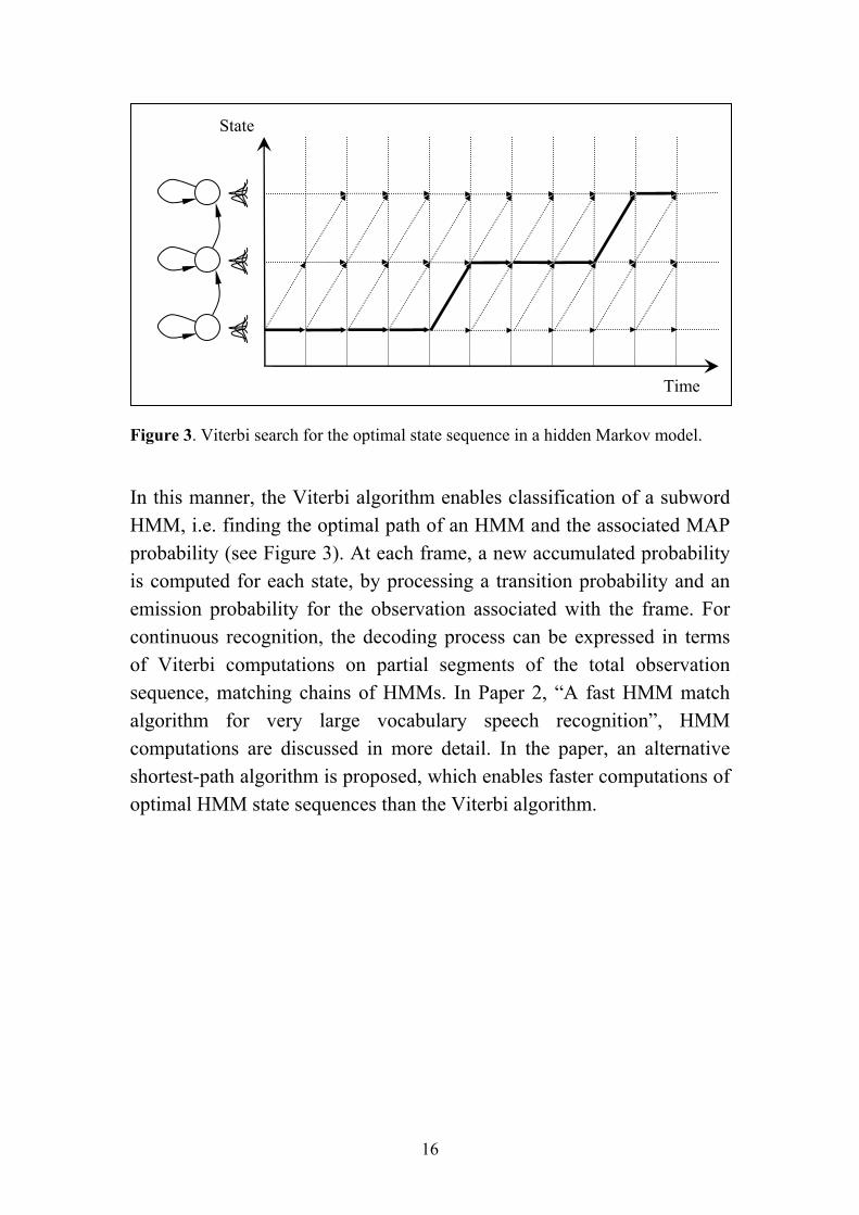
Figure 3. Viterbi search for the optimal state sequence in a hidden Markov model.

In this manner, the Viterbi algorithm enables classification of a subword HMM, i.e. finding the optimal path of an HMM and the associated MAP probability (see Figure 3). At each frame, a new accumulated probability is computed for each state, by processing a transition probability and an emission probability for the observation associated with the frame. For continuous recognition, the decoding process can be expressed in terms of Viterbi computations on partial segments of the total observation sequence, matching chains of HMMs. In Paper 2, “A fast HMM match algorithm for very large vocabulary speech recognition”, HMM computations are discussed in more detail. In the paper, an alternative shortest-path algorithm is proposed, which enables faster computations of optimal HMM state sequences than the Viterbi algorithm.

16

5 Weighted finite-state transducers In Chapter 3, we described how HMMs can be applied as classifiers of subword acoustic-phonetic units. In Chapter 4 we described how the decoding problem was formulated as a product of HMMs (acoustic models) and the a priori knowledge sources. As mentioned in the previous sections, these knowledge sources represent lexical and syntactical knowledge, e.g. pronunciation models, phonetic context-dependency models and language models. Similar to hidden Markov models, a major part of the a priori models are statistical models obtained from training on large sets of data. Other a priori models are represented by explicit knowledge or rules. In order to combine these knowledge sources into a single model, an additional concept is applied – the theory of weighted finite-state transducers (WFST). Weighted finite-state state transducers have recently been applied for this purpose (Mohri 1997, Aubert 2000, Ljolje et al. 2000, Zue et al. 2000, Seward 2001, Mohri et al. 2002, Seward 2004). There are three main incentives for this approach. First, it enables many of the knowledge sources of the decoding process to be modeled efficiently by a single framework. Second, it enables the application of a broad class of generic automata operations and algorithms, many of which have been developed at AT&T Labs Research (Mohri 1997, Pereira and Riley 1997, Mohri 2000, Mohri 2001, Mohri 2002). These operations constitute powerful tools to transform, merge and optimize these finite-state machines for improved performance. Third, it enables a straightforward separation of data and algorithms in the decoder. For instance, whether a decoder applies bigrams, or higher order n-grams (see Chapter 6.2), uses triphones across words or not (see Chapter 7), are typical aspects that can be separated from the implementation of the recognizer, and be completely modeled by transducers.

5.1 Definitions The definitions of weighted transducers and automata and their related weighted operations are based on the notion of semirings (Kuich and Salomaa 1986). A semiring, = ( , ⊕, ⊗, 1,0 ) is a ring that may lack

17

negation. It is defined as a set , with two identity elements 1,0 and two binary operators ⊕ and ⊗, (commonly interpreted as addition and multiplication, respectively). The operators ⊕ and ⊗ are defined to satisfy the following conditions: 1. Additive and multiplicative associativity: For all a,b,c ∈ , (a ⊕ b) ⊕ c = a ⊕ (b ⊕ c) and (a ⊗ b) ⊗ c = a ⊗ (b ⊗ c) 2. Additive commutativity: For all a,b ∈ , a ⊕ b = b ⊕ a 3. Left and right distributivity: For all a,b,c ∈ , a ⊗ (b ⊕ c) = (a ⊗ b) ⊕ (a ⊗ c) (b ⊕ c) ⊗ a = (b ⊗ a) ⊕ (c ⊗ a) 4. 0 is an annihilator, such that 0 0 0a a⊗ = ⊗ = Weighted finite-state transducers constitute a general class of finite-state automata. A WFST is defined by T = (Σ, Ω, Q, E, I, F, λ, ρ) over a semiring = ( , ⊕, ⊗, 1,0 ), where Σ is an input alphabet, Ω is an output alphabet, Q is a finite-set of states, E is finite set of weighted transitions, I ∈Q is an initial state, F ⊆ Q is a set of final states, λ is an initial weight function λ: I → and ρ is an final weight function ρ:F → . λ maps an optional weight to the initial state, and ρ maps a weight to the final states. For all other states, λ and ρ return the identity element 1 . A transition is represented by an arc, from a source state, to a destination state, with an associated weight, an input label and an output label. We define the weight function as w:e → , i.e. w[e] is the weight of a transition e. Valid input and output labels are symbols from the input and output alphabets respectively, and the empty symbol ε. Similarly, we define the label functions i: e → (Σ ∪ ε) , and o: e → (Ω ∪ ε), such that i[e] and o[e] denote the input and the output of a transition e ∈ E. A transition is defined by e ∈ E ⊆ Q × (Σ ∪ ε) × (Ω ∪ ε) × × Q.

18

A special case of weighted finite-state transducers without output alphabets are weighted finite-state acceptors (WFSA). A WFSA is defined by A = (Σ, Q, E, I, F, λ, ρ) over a semiring = ( , ⊕, ⊗, 1,0 ). Transitions have an associated weight and an input label, but no output label. Thus, a transition is defined by e ∈ E ⊆ Q × (Σ ∪ ε) × × Q. Whereas WFSTs represents weighted transductions of languages, WFSAs represents weighted acceptors of languages. Alternatively, the label alphabet of a WFSA can also be interpreted as an output alphabet. In this interpretation, a WFSA is regarded as a weighted emitter of a language.

A path π in a WFST or WFSA denotes a single transition or a consecutive series of transitions e1…ek. Similar to single transitions, the source state of a path denotes the first state, whereas the destination state denotes the last state. A destination state is reachable from a source state, if there is a path from the source state to the destination state. The weight w[π] of a path π = e1…ek is given by the ⊗-product of the weight of its constituent transitions.

[ ] [ ] [ ] [ ]1 2w = w e w e w eπ ⊗ ⊗ ⊗… k (14)

For a path π, let the functions s[π] and d[π] denote the source state and the destination state, respectively. If a path involves the initial state or a final state, the corresponding initial and final weight are included in the weight calculation. A successful path e1…ek is a path from the initial state I ∈Q to a final state d[ek] ∈ F. Hence, the weight is given by [ ] [ ] [ ] [ ] [ ] [ ]1 1 2 kw = (s e ) w e w e w e (d e )π λ ρ⊗ ⊗ ⊗ ⊗ ⊗… k (15)

Let a sequence denote a series of symbols obtained by concatenation of transition labels. Hence, a transducer path has an input sequence and an output sequence, given by concatenation of the input labels and output labels, respectively. As with the weight function, the label functions i and o are also defined for paths to return sequences, such that i: π → (Σ* ∪ ε) and o: π → (Ω* ∪ ε). Hence, for a path π = (e1, e2, …, ek), the input sequence is given by i[π]= (i[e1], i[e1],…, i[ek]). Likewise, for a

19

transducer path π = (e1, e2, …, ek), the output sequence is given by o[π]= (o[e1], o[e1],…, o[ek]).

Thus, for WFSTs and WFSAs, extension of paths is performed by the ⊗-operator for the weights, and by concatenation for the labels (see Table 1).

Table 1. Semiring operations and their usage.

Weight operator

Usage

⊗ Extension of a path

⊕ Accumulation of a set of paths

The weight of a set of paths is given by the ⊕-operator. This is used to compute the weight of sequences that correspond to a set of paths. For a finite set of paths П = π1, π1, …, πn, the associated weight is defined by the ⊕-sum of the weights of the constituent paths:

[ ] ( ([ ]) ( ) ( [w s wπ

])dλ π π ρ∈Π

Π = ⊗ ⊗⊕ π (16)

Depending on the semiring applied, WFSAs and WFSTs model different languages and language transductions, with different meaning of the weight operators. Table 2 shows an example of different semirings. In Chapter 4, the decoding problem was described in terms of a stochastic model. Modeled in the transducer framework, this implies the probability semiring (see Table 2), where weights denote probabilities and the operators ⊕ and ⊗ denote normal addition and multiplication, respectively. In this case, computation of weights of paths is analogous to the Forward algorithm in the linear domain, i.e. paths are extended by multiplication and accumulated by addition. However, in order to avoid numerical underflow in speech decoders, computations are typically performed in the logarithmic domain, where weights represent the negative logarithm of real scalars. This corresponds to a change from the probability

20

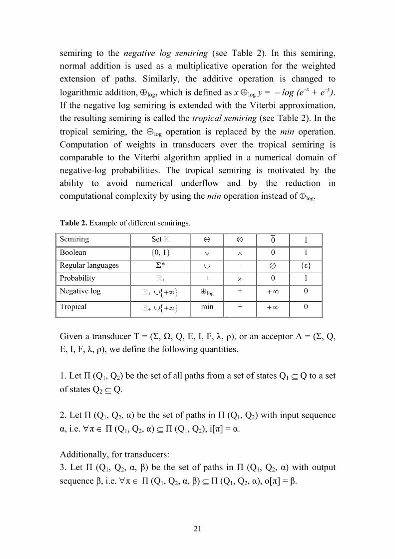
semiring to the negative log semiring (see Table 2). In this semiring, normal addition is used as a multiplicative operation for the weighted extension of paths. Similarly, the additive operation is changed to logarithmic addition, ⊕log, which is defined as x ⊕log y = – log (e–x + e–y). If the negative log semiring is extended with the Viterbi approximation, the resulting semiring is called the tropical semiring (see Table 2). In the tropical semiring, the ⊕log operation is replaced by the min operation. Computation of weights in transducers over the tropical semiring is comparable to the Viterbi algorithm applied in a numerical domain of negative-log probabilities. The tropical semiring is motivated by the ability to avoid numerical underflow and by the reduction in computational complexity by using the min operation instead of ⊕log.

Table 2. Example of different semirings.

Semiring Set ⊕ ⊗ 0 1 Boolean 0, 1 ∨ ∧ 0 1 Regular languages Σ* ∪ · ∅ ε Probability + + × 0 1 Negative log + ∪ +∞ ⊕log + ∞+ 0

Tropical + ∪ +∞ min + ∞+ 0

Given a transducer T = (Σ, Ω, Q, E, I, F, λ, ρ), or an acceptor A = (Σ, Q, E, I, F, λ, ρ), we define the following quantities. 1. Let П (Q1, Q2) be the set of all paths from a set of states Q1 ⊆ Q to a set of states Q2 ⊆ Q. 2. Let П (Q1, Q2, α) be the set of paths in П (Q1, Q2) with input sequence α, i.e. ∀π ∈ П (Q1, Q2, α) ⊆ П (Q1, Q2), i[π] = α. Additionally, for transducers: 3. Let П (Q1, Q2, α, β) be the set of paths in П (Q1, Q2, α) with output sequence β, i.e. ∀π ∈ П (Q1, Q2, α, β) ⊆ П (Q1, Q2, α), o[π] = β.

21

The weight of an input sequence α ∈ Σ*, for an acceptor A = (Σ, Q, E, I, F, λ, ρ) is defined by:

( )π Π(I,F,α)

A α λ(s[π]) w[π] ρ(d[π])∈

= ⊗ ⊗⊕ (17)

The weight of a sequence pair (α, β), for a transducer T = (Σ, Ω, Q, E, I, F, λ, ρ), where α ∈ Σ* is an input sequence and β ∈ Ω* is an output sequence is defined by:

( )π Π(I,F,α,β)

T α,β λ(s[π]) w[π] ρ(d[π])∈

= ⊗ ⊗⊕ (18)

Hence, T (α, β) defines the weight associated with the transduction α → β, for any input sequence α and output sequence β.

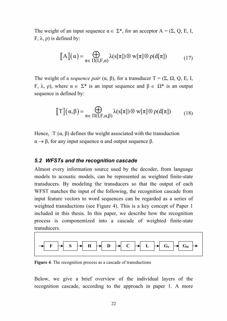
5.2 WFSTs and the recognition cascade Almost every information source used by the decoder, from language models to acoustic models, can be represented as weighted finite-state transducers. By modeling the transducers so that the output of each WFST matches the input of the following, the recognition cascade from input feature vectors to word sequences can be regarded as a series of weighted transductions (see Figure 4). This is a key concept of Paper 1 included in this thesis. In this paper, we describe how the recognition process is componentized into a cascade of weighted finite-state transducers.

S H D C L GI GII F

Figure 4. The recognition process as a cascade of transductions

Below, we give a brief overview of the individual layers of the recognition cascade, according to the approach in paper 1. A more

22

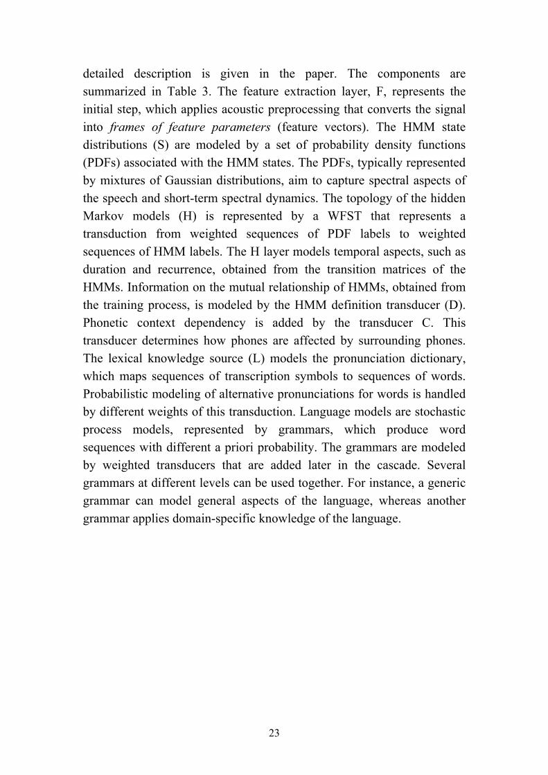
detailed description is given in the paper. The components are summarized in Table 3. The feature extraction layer, F, represents the initial step, which applies acoustic preprocessing that converts the signal into frames of feature parameters (feature vectors). The HMM state distributions (S) are modeled by a set of probability density functions (PDFs) associated with the HMM states. The PDFs, typically represented by mixtures of Gaussian distributions, aim to capture spectral aspects of the speech and short-term spectral dynamics. The topology of the hidden Markov models (H) is represented by a WFST that represents a transduction from weighted sequences of PDF labels to weighted sequences of HMM labels. The H layer models temporal aspects, such as duration and recurrence, obtained from the transition matrices of the HMMs. Information on the mutual relationship of HMMs, obtained from the training process, is modeled by the HMM definition transducer (D). Phonetic context dependency is added by the transducer C. This transducer determines how phones are affected by surrounding phones. The lexical knowledge source (L) models the pronunciation dictionary, which maps sequences of transcription symbols to sequences of words. Probabilistic modeling of alternative pronunciations for words is handled by different weights of this transduction. Language models are stochastic process models, represented by grammars, which produce word sequences with different a priori probability. The grammars are modeled by weighted transducers that are added later in the cascade. Several grammars at different levels can be used together. For instance, a generic grammar can model general aspects of the language, whereas another grammar applies domain-specific knowledge of the language.

23

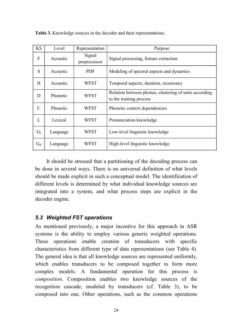
Table 3. Knowledge sources in the decoder and their representations.

KS Level Representation Purpose

F Acoustic Signal

preprocessor Signal processing, feature extraction

S Acoustic PDF Modeling of spectral aspects and dynamics

H Acoustic WFST Temporal aspects; duration, recurrence

D Phonetic WFST Relation between phones, clustering of units according to the training process

C Phonetic WFST Phonetic context dependencies

L Lexical WFST Pronunciation knowledge

GI Language WFST Low-level linguistic knowledge

GII Language WFST High-level linguistic knowledge

It should be stressed that a partitioning of the decoding process can be done in several ways. There is no universal definition of what levels should be made explicit in such a conceptual model. The identification of different levels is determined by what individual knowledge sources are integrated into a system, and what process steps are explicit in the decoder engine.

5.3 Weighted FST operations As mentioned previously, a major incentive for this approach in ASR systems is the ability to employ various generic weighted operations. These operations enable creation of transducers with specific characteristics from different type of data representations (see Table 4). The general idea is that all knowledge sources are represented uniformly, which enables transducers to be composed together to form more complex models. A fundamental operation for this process is composition. Composition enables two knowledge sources of the recognition cascade, modeled by transducers (cf. Table 3), to be composed into one. Other operations, such as the common operations

24

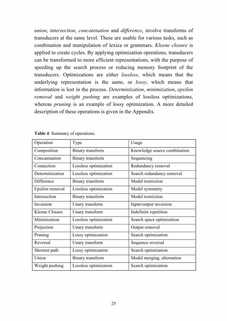
union, intersection, concatenation and difference, involve transforms of transducers at the same level. These are usable for various tasks, such as combination and manipulation of lexica or grammars. Kleene closure is applied to create cycles. By applying optimization operations, transducers can be transformed to more efficient representations, with the purpose of speeding up the search process or reducing memory footprint of the transducers. Optimizations are either lossless, which means that the underlying representation is the same, or lossy, which means that information is lost in the process. Determinization, minimization, epsilon removal and weight pushing are examples of lossless optimizations, whereas pruning is an example of lossy optimization. A more detailed description of these operations is given in the Appendix.

Table 4. Summary of operations.

Operation Type Usage

Composition Binary transform Knowledge source combination

Concatenation Binary transform Sequencing

Connection Lossless optimization Redundancy removal

Determinization Lossless optimization Search redundancy removal

Difference Binary transform Model restriction

Epsilon removal Lossless optimization Model symmetry

Intersection Binary transform Model restriction

Inversion Unary transform Input/output inversion

Kleene Closure Unary transform Indefinite repetition

Minimization Lossless optimization Search space optimization

Projection Unary transform Output removal

Pruning Lossy optimization Search optimization

Reversal Unary transform Sequence reversal

Shortest path Lossy optimization Search optimization

Union Binary transform Model merging, alternation

Weight pushing Lossless optimization Search optimization

25

6 Language modeling In this chapter two classes of grammars used in this thesis are briefly described.

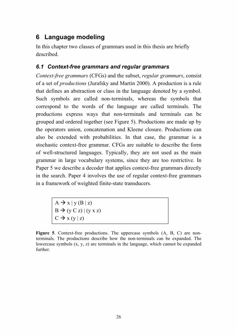
6.1 Context-free grammars and regular grammars Context-free grammars (CFGs) and the subset, regular grammars, consist of a set of productions (Jurafsky and Martin 2000). A production is a rule that defines an abstraction or class in the language denoted by a symbol. Such symbols are called non-terminals, whereas the symbols that correspond to the words of the language are called terminals. The productions express ways that non-terminals and terminals can be grouped and ordered together (see Figure 5). Productions are made up by the operators union, concatenation and Kleene closure. Productions can also be extended with probabilities. In that case, the grammar is a stochastic context-free grammar. CFGs are suitable to describe the form of well-structured languages. Typically, they are not used as the main grammar in large vocabulary systems, since they are too restrictive. In Paper 5 we describe a decoder that applies context-free grammars directly in the search. Paper 4 involves the use of regular context-free grammars in a framework of weighted finite-state transducers.

A x | y (B | z) B (y C z) | (y x z) C x (y | z)

Figure 5. Context-free productions. The uppercase symbols (A, B, C) are non-terminals. The productions describe how the non-terminals can be expanded. The lowercase symbols (x, y, z) are terminals in the language, which cannot be expanded further.

26

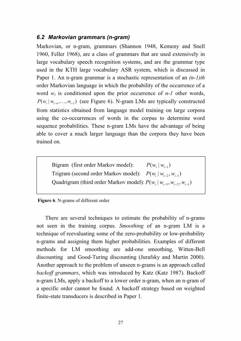
6.2 Markovian grammars (n-gram) Markovian, or n-gram, grammars (Shannon 1948, Kemeny and Snell 1960, Feller 1968), are a class of grammars that are used extensively in large vocabulary speech recognition systems, and are the grammar type used in the KTH large vocabulary ASR system, which is discussed in Paper 1. An n-gram grammar is a stochastic representation of an (n-1)th order Markovian language in which the probability of the occurrence of a word wi is conditioned upon the prior occurrence of n-1 other words,

1( | , , )i i n iP w w w− … − (see Figure 6). N-gram LMs are typically constructed from statistics obtained from language model training on large corpora using the co-occurrences of words in the corpus to determine word sequence probabilities. These n-gram LMs have the advantage of being able to cover a much larger language than the corpora they have been trained on.

1

2 1

3 2 1

Bigram (first order Markov model): ( | )Trigram (second order Markov model): ( | , )Quadrigram (third order Markov model): ( | , , )

i i

i i i

i i i i

P w wP w w wP w w w w

−

− −

− − −

Figure 6. N-grams of different order.

There are several techniques to estimate the probability of n-grams

not seen in the training corpus. Smoothing of an n-gram LM is a technique of reevaluating some of the zero-probability or low-probability n-grams and assigning them higher probabilities. Examples of different methods for LM smoothing are add-one smoothing, Witten-Bell discounting and Good-Turing discounting (Jurafsky and Martin 2000). Another approach to the problem of unseen n-grams is an approach called backoff grammars, which was introduced by Katz (Katz 1987). Backoff n-gram LMs, apply a backoff to a lower order n-gram, when an n-gram of a specific order cannot be found. A backoff strategy based on weighted finite-state transducers is described in Paper 1.

27

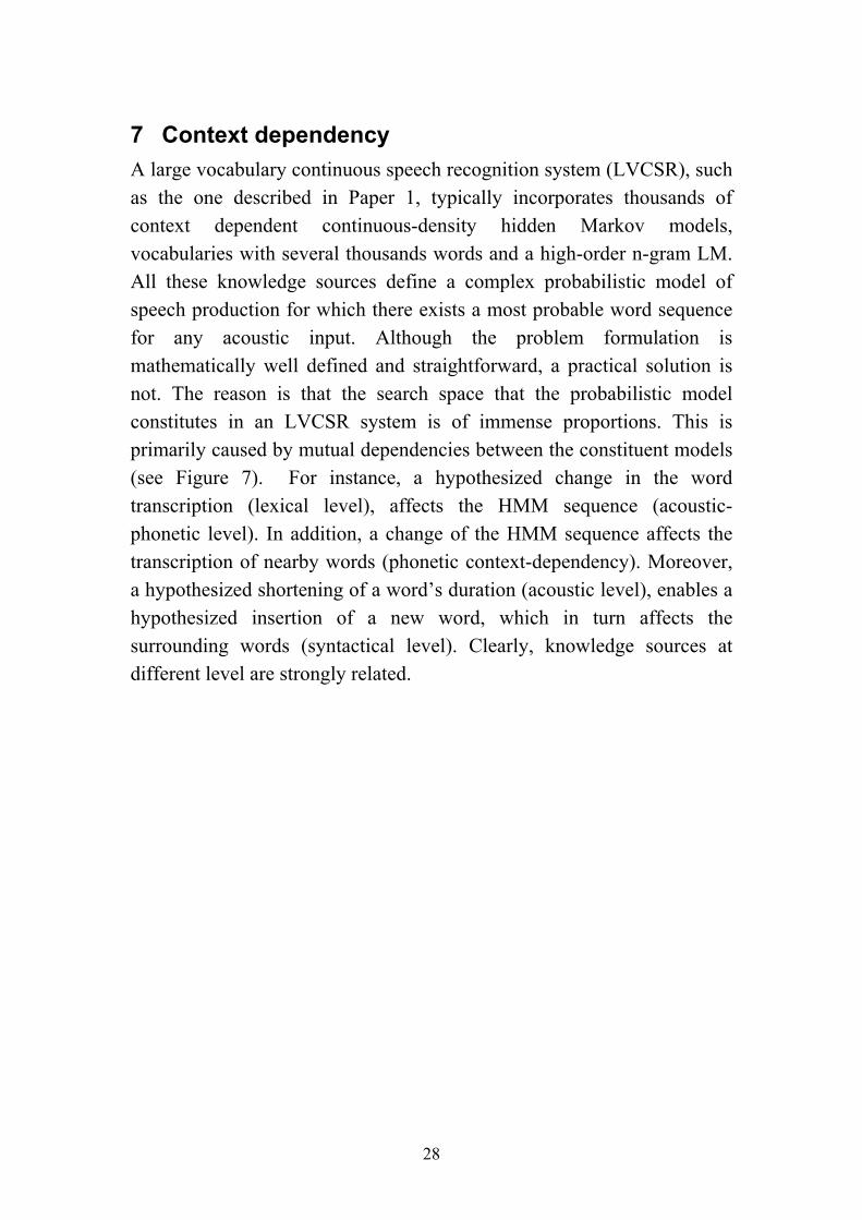
7 Context dependency A large vocabulary continuous speech recognition system (LVCSR), such as the one described in Paper 1, typically incorporates thousands of context dependent continuous-density hidden Markov models, vocabularies with several thousands words and a high-order n-gram LM. All these knowledge sources define a complex probabilistic model of speech production for which there exists a most probable word sequence for any acoustic input. Although the problem formulation is mathematically well defined and straightforward, a practical solution is not. The reason is that the search space that the probabilistic model constitutes in an LVCSR system is of immense proportions. This is primarily caused by mutual dependencies between the constituent models (see Figure 7). For instance, a hypothesized change in the word transcription (lexical level), affects the HMM sequence (acoustic-phonetic level). In addition, a change of the HMM sequence affects the transcription of nearby words (phonetic context-dependency). Moreover, a hypothesized shortening of a word’s duration (acoustic level), enables a hypothesized insertion of a new word, which in turn affects the surrounding words (syntactical level). Clearly, knowledge sources at different level are strongly related.

28

Bigrams

Figure 7. Phonetic and syntactic context dependencies. The figure illustrates the partial transcription [V A: R I: D E:] of the utterance “det var i det samman–hanget” (Eng: “it was in that context”). The upper subfigure illustrates triphone recognition with a bigram LM. Since there is no n-phone expansion across words in this case, triphones are used only within words with a length of three phones or more. The lower subfigure illustrates triphone recognition with a trigram LM and cross word n-phone expansion. In this more complex case, the pronunciation of words is determined by the surrounding words.

V A: R I: D E:

V A: R I: D E:

Triphone recognition without cross-word context expansion + bigram LM

Triphone recognition with cross-word context expansion + trigram LM

Monophone

Diphones

Triphone

P(w3|w2)

P(w2|w1)

w1 w2 w3

Trigrams

P(w2|w0,w1)

P(w3|w1,w2)

P(w4|w2,w3)

w1 w2 w3

Triphones

29

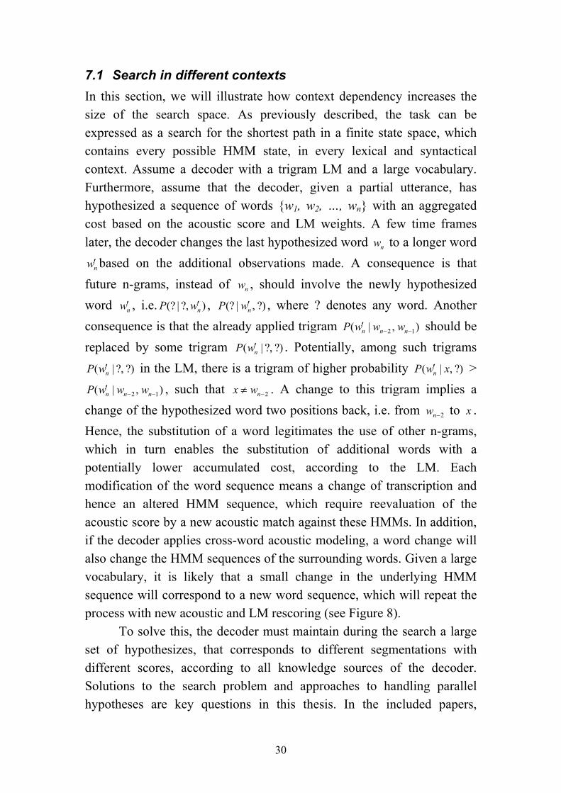
7.1 Search in different contexts In this section, we will illustrate how context dependency increases the size of the search space. As previously described, the task can be expressed as a search for the shortest path in a finite state space, which contains every possible HMM state, in every lexical and syntactical context. Assume a decoder with a trigram LM and a large vocabulary. Furthermore, assume that the decoder, given a partial utterance, has hypothesized a sequence of words w1, w2, …, wn with an aggregated cost based on the acoustic score and LM weights. A few time frames later, the decoder changes the last hypothesized word to a longer word

based on the additional observations made. A consequence is that future n-grams, instead of , should involve the newly hypothesized word , i.e. ,

nw

nw′

nw

nw′ (? | ?, )nP w′ (? | , ?)nP w′ , where ? denotes any word. Another consequence is that the already applied trigram 2 1( | , )n n nP w w w− −′ should be replaced by some trigram ( | ?, ?)nP w′ . Potentially, among such trigrams

in the LM, there is a trigram of higher probability > , such that

( | ?, ?)nP w′ ( | , ?)nP w x′

2 1( | , )n n nP w w w− −′ 2nx w −≠ . A change to this trigram implies a change of the hypothesized word two positions back, i.e. from to 2nw − x . Hence, the substitution of a word legitimates the use of other n-grams, which in turn enables the substitution of additional words with a potentially lower accumulated cost, according to the LM. Each modification of the word sequence means a change of transcription and hence an altered HMM sequence, which require reevaluation of the acoustic score by a new acoustic match against these HMMs. In addition, if the decoder applies cross-word acoustic modeling, a word change will also change the HMM sequences of the surrounding words. Given a large vocabulary, it is likely that a small change in the underlying HMM sequence will correspond to a new word sequence, which will repeat the process with new acoustic and LM rescoring (see Figure 8).

To solve this, the decoder must maintain during the search a large set of hypothesizes, that corresponds to different segmentations with different scores, according to all knowledge sources of the decoder. Solutions to the search problem and approaches to handling parallel hypotheses are key questions in this thesis. In the included papers,

30

different solutions to the search problem are proposed, which are adapted to different decoding tasks with different requirements.

Acoustic rescoring Hypothesize a different HMM in the sequence

New word sequence

LM rescoring Apply different n-grams

New word sequence

Figure 8. The search space as a cycle of acoustic and LM rescoring.

31

8 Summary of papers This thesis, including the proposed methods and algorithms, as well as the design and the implementation of the three ASR systems which this work is based on, is the result of the author’s own work.

This section contains a summary of the papers included in this thesis. The main focus of this work is on the first two papers, “The KTH Large Vocabulary Continuous Speech Recognition System” and “A fast HMM Match Algorithm for Very Large Vocabulary Speech Recognition”, which relate to large vocabulary speech recognition. The other three papers, “Low-Latency Incremental Speech Transcription in the Synface Project”, “Transducer optimizations for tight-coupled decoding” and “A Tree-Trellis N-best Decoder for Stochastic Context-Free Grammars” focus on other aspects of speech recognition with more limited tasks.

32

8.1 Paper 1. The KTH Large Vocabulary Continuous Speech Recognition System.

This paper presents the KTH system for large vocabulary speech recognition (LVCSR). The system is based on weighted finite-state transducers, for the search as well as the representation of all knowledge sources used by the decoder. This work has focused on building a system aimed at handling online recognition tasks with large vocabularies, in real time. Particular attention has been paid to providing support for specific tasks, such as dictation and live transcription. These criteria impose additional requirements on the system. The described decoder incorporates a time-synchronous search algorithm with the capability of emitting partial results (word by word) during the search and a backtracking strategy for efficient generation of output sequences. A strategy for managing long input sequences is also proposed, which enables several consecutive search passes to be performed without halting the audio sampling process. The acoustic modeling is handled by context-dependent continuous-density hidden Markov models, with Gaussian Mixture distributions. The recognizer has full support for cross-word n-phone expansion. Weighted finite-state transducers are used for the representation of all components, including lexica, language models, phonetic context-dependency and the topology of hidden Markov models. Such components are combined and optimized using general WFST operations to obtain a weighted transduction directly from input feature vectors to word sequences. The primary principle for language modeling in the system is back-off n-grams of arbitrary order. However, the system can handle any type of language model that can be modeled or approximated by weighted finite-state transducers.

33

8.2 Paper 2. A Fast HMM Match Algorithm for Very Large Vocabulary Speech Recognition

This work presents a HMM matching procedure that aims to reduce the overall computational complexity of the search in large vocabulary speech recognition systems. In such systems, the search over context-dependent continuous-density hidden Markov models and state-probability computations account for a considerable part of the total decoding time. This is especially apparent in complex tasks that incorporate large vocabularies and n-grams of high order, since these impose a high degree of context dependency and HMMs have to be treated differently in each context. Specifically, this means that a single HMM might have to be hypothesized and matched multiple times during an utterance, but also that such matches might overlap or coincide in time, due to the context dependencies of the higher level models.

If the start time is given, the Viterbi algorithm is an efficient method for computation of HMM emission likelihoods. The algorithm’s dynamic programming aspects enable an incremental extension to longer segments (increased path duration), by utilization of previous computations. This is applied by decoders to hypothesize different segmentations of the same HMM. However, the Viterbi algorithm relies on the start time to be determined for the computation of an optimal state sequence. By hypothesizing the time boundaries differently so that the associated HMM emission probabilities account for different segments of the same observation sequence, the corresponding optimal paths are potentially partially or completely disjoint. If a segment with a different start time is hypothesized, a separate Viterbi search is required.

In this paper, a novel HMM search algorithm is presented, which enables both the start time and the end time of an HMM path to be hypothesized using a single search. Instead of applying simple extension of paths as with the Viterbi algorithm, optimal state sequences are computed by comparisons of regions of space-time.

The proposed HMM match algorithm enables an efficient decoupling of the acoustic match from the main search. Instead of computing a large amount of likelihoods for different alignments of each HMM, the proposed method computes all alignments, but more

34

efficiently than with the Viterbi algorithm. Each HMM is matched only once against any time interval. The associated emission likelihoods can be instantly looked up on demand by the main search algorithm that involves the lexical and syntactical knowledge.

There are three advantages of this approach over standard integrated decoding with the Viterbi algorithm. First, it enables a straightforward distribution of the decoding process over multiple processors, since it enables the HMM match to be performed autonomously on one processor, whereas the main search can be executed on a second processor. Second, each CD-HMM is matched only once against any time interval, thus getting rid of redundant computations that are involved in an integrated search. Third, the HMM match algorithm is optimized by taking advantage of a specific HMM topology to share partial time-warping evaluations across successive time intervals in a parallel manner.

35

8.3 Paper 3. Low-Latency Incremental Speech Transcription in the Synface Project

In this paper, a real-time decoder for low-latency online speech transcription is presented. This decoder was the initial decoder developed in the Synface project (Granström et al. 2002). The paper addresses specific issues related to HMM-based incremental phone classification with real-time constraints. The target application in this case, is a telephony system aimed to support hard-of-hearing people in the use of conventional telephony. This is done by providing lip reading support to the user with a synthetic talking face. The task of the decoder is to translate the incoming speech signal to parameters, which enable the synthetic face to articulate in synchrony with the speech signal that the user receives over the telephone.

Specifically, the system specification adds the following requirements to conventional HMM decoding.

• The recognizer must produce partial output sequences, incrementally during the utterance.

• Real-time constraints: output must be emitted time-synchronously

such that any delay is fixed and determinable. • Output symbols cannot be changed once emitted.

The use of HMMs to solve such a recognition task involves several challenges. In this case, it is not sufficient to periodically emit the most promising partial hypothesis as output. The reason is that a hypothesis, which at a point of time during the decoding process has the highest accumulated likelihood, very well can prove to be incorrect according to the probabilistic model, when additional input frames have been observed. This occurs when another hypothesis, which corresponds to a different path in the search space, as well as a different symbol sequence, takes the role of the currently best hypothesis.

In recognition systems that produce incremental output this is typically handled by making a correction of the emitted output so that it

36

corresponds to the currently best hypothesis. However, corrections are not possible in this case, since any incorrectly emitted output already has been realized for the user as articulatory movements in the synthetic face.

The approach taken in this work is to stream the incoming speech signal to the user with a fixed delay, while at the same time streaming it to the decoder without delay. The decoder can utilize that time gap, or latency, for hypothesis look-ahead. The method enables the decoder to produce more robust output by looking ahead on the speech segments that the user has not yet received. By applying hypothesis look-ahead, certain errors can be avoided.

The decoding algorithm proposed in this work enables a trade-off to be made between improved recognition accuracy and reduced latency. By accepting a longer latency per output increment, more time can be ascribed to hypothesis look-ahead, thus improving classification accuracy. This work also shows that it is possible to obtain the same recognition results as with non-incremental decoding, by applying hypothesis look-ahead.

37

8.4 Paper 4. Transducer optimizations for tight-coupled decoding.

In this paper we survey the benefits of various automata optimizations in tight-coupled decoding with regular languages. As described previously, regular grammars are less suitable for large vocabulary tasks, due to their restrictive nature. However, their ability to capture the syntax and long-range dependencies of a language and the fact that they can be described by context-free rules, make them useful for several recognition tasks. The search structures adopted in this paper are statically built integrated transducers. They are composed from a pronunciation dictionary and a regular language model, to obtain a mapping from sequences of HMM labels to sequences of words. The paper evaluates the effects of optimizations, such as minimization in terms of recognition performance and the size of the integrated search structures. Moreover, a dual-pass approach is applied, which is based on decomposition of integrated transducers into two layers over an intermediate symbol alphabet. Finally, a method to partially simulate bi-directional determinism of transducers is evaluated. The paper shows, that using these optimizations, a search net of more than 2 million states, can be reduced in size to less than 200 thousand states without losing any information. The small size also enables a more efficient search that improves recognition accuracy.

38

8.5 Paper 5. A tree-trellis N-best decoder for stochastic context-free grammars

This work describes a speech recognizer for stochastic context-free grammars. Different aspects of the decoder are described, such as the search and the strategy for pruning. This recognizer was implemented with the Ace speech recognition toolkit, which is briefly described in the paper. One purpose of this paper was to survey the possibilities of combining alternative search structures for the representation of regular and irregular grammars. Context-free irregular grammars cannot be represented by regular automata. There are, however, other classes of finite-state machines, such as recursive transition networks (Woods 1970) and pushdown automata (Hopcroft and Ullman 1979), capable of representing irregular grammars. In this work, we apply a framework of stochastic pushdown automata, which is an extension of pushdown automata that handles stochastic context-free grammars. Apart from the ability to model irregular grammars, these devices are less effective as search structures than regular automata, since they require an auxiliary stack memory for traversing nodes. Another difference is that pushdown automata generally constitute a more memory efficient representation than the regular automata equivalents. For the purpose of adding support for both these classes of finite-state machines, the decoder described in this work applies an implementation of stochastic pushdown automata suited for dynamic conversion to regular finite-state automata (acceptors). Grammars are initially represented as pushdown automata. For irregular grammars this representation can be used by the decoder with an auxiliary stack. However, if the grammar is regular, the search structure is expanded to an equivalent acceptor, which eliminates the need for the auxiliary stack. In this sense, the paper aims at describing a possible solution to combining different grammar representations under a single framework, rather than quantifying their relative advantages.

39

9 References Aho, A., Hopcroft, E., and Ullman, D.,1974, The design and analysis of

computer algorithms, Addison Wesley. Reading, Massachusetts.

Alleva, F., Hon, H., Huang, X., Hwang, M., Rosenfeld, R., and Weide, R.,1992, Applying SPHINX-II to the DARPA Wall Street Journal CSR Task, Proc. of DARPA Speech and Natural Language Workshop pp. 393-398.

Aubert, X. L.,2000, A brief overview of decoding techniques for large vocabulary continuous speech recognition, Proc. of Automatic Speech Recognition workshop, 1, pp. 91-96.

Baker,1975, Stochastic Modeling for Automatic Speech Understanding, Speech Recognition - Invited papers presented at the 1974 IEEE Symposium, pp. 521-542, D. R. Reddy, Ed. Academic press. New York.

Baum, L. E. and Eagon, J. A.,1967, An inequality with applications to statistical estimation for probabilistic functions of Markov processes and to a model for ecology, Bulletin of American Mathematical Society, 73(3), pp. 360-363.

Baum, L. E. and Petrie, T.,1966, Statistical inference for prbabilistic functions of finite-state Markov chains, Annals of Mathematical Statistics, 37(6), pp. 1554-1563.

Beaufays, F., Sankar, A., Williams, S., and Weintraub, M.,2003, Learning linguistically valid pronunciations from acoustic data, Proc. of Eurospeech pp. 2593-2596. Geneva

Bellman, R.,1957, Dynamic Programming, Princeton University Press. Princeton.

Bellman, R.,1958, On a routing problem, Proc. of Quarterly of Applied Mathematics, 16,

Beyerlein, P., Ullrich, M., and Wilcox, P.,1997, Modeling and Decoding of Crossword Context Dependent Phones in the Philips Large Vocabulary Continuous Speech Recognition System, Proc. of European Conf. on Speech Communication and Technology pp. 1163-1166.

40

Black, A., Lenzo, K., and Pagel, V.,1998, Issues in building general letter to sound rules, Proc. of ESCA Workshop on Speech Synthesis pp. 77-80.

Dijkstra, E. W.,1959, A note on two problems in connection with graphs, Numerische Mathematik, 1, pp. 269-271.

Feller, W.,1968, Introduction to probability theory and its applications, 1, third ed, John Wiley & Sons. New York.

Ford, L. R. and Fulkerson, D. R.,1956, Maximal flow through a network, Canadian Journal of Mathematics, pp. 399-404.

Forney, G. D.,1973, The Viterbi Algorithm, Proc. of IEEE, 61, pp. 268-278.

Granström, B., Karlsson, I., and Spens, K.-E.,2002, Synface - a project presentation, Proc. of Fonetik, TMH-QPSR, 44, pp. 93-96.

Holter, T.,1997, Maximum likelihood modelling of pronunciation in automatic speech recognition, Ph.D. Thesis, The Norwegian University of Science and Technology. Trondheim.

Hopcroft, J. and Ullman, J.,1979, Introduction to automata theory, languages and computation, Addison-Wesley. Reading, Massachusetts.

Jelinek, F.,1976, Continuous Speech Recognition by Statistical Methods, Procedings of IEEE, 64, pp. 532-556.

Jelinek, F.,1998, Statistical Methods for speech recognition, MIT Press. Cambridge, Massachusetts.

Jurafsky, D. and Martin, J.,2000, Speech and language processing, Prentice Hall. Upper Saddle River, NJ.

Katz, S. M.,1987, Estimation of probabilities from sparse data for the language model component of a speech recognizer, Proc. of IEEE Transactions on Acoustics, Speech and Signal Processing, 35(3), pp. 400-401.

Kemeny, J. G. and Snell, J. L.,1960, Finite Markov Chains, Van Nostrand. Princeton.

Kuich, W. and Salomaa, A.,1986, Semirings, Automata, Languages, 5 Springer-Verlag. Berlin.

41

Lee, K. F.,1990, Context dependent phonetic hidden Markov models for continuous speech recognition, Proc. of IEEE Trans. ASSP, 38(4), pp. 599-609.

Ljolje, A., Riley, M., Hindle, D., and Sproat, R.,2000, The AT&T LVCSR-2000 System, Proc. of NIST Large Vocabulary Conversational Speech Recognition Workshop

Mohri, M.,1997, Finite-state transducers in language and speech processing, Computational linguistics, 23, pp. 269-312.

Mohri, M.,2000, Minimization algorithms for sequential transducers, Theoretical Computer Science, 234, pp. 177-201.

Mohri, M.,2001, A Weight Pushing Algorithm for Large Vocabulary Speech Recognition, Proc. of European Conference on Speech Communication and Technology

Mohri, M.,2002, Generic Epsilon-Removal and Input Epsilon-Normalization Algorithms for Weighted Transducers, International Journal of Foundations of Computer Science, 13, pp. 129-143.

Mohri, M., Pereira, F., and Riley, M.,2002, Weighted Finite-State Transducers in Speech Recognition, Computer Speech and Language, 1, pp. 69-88.

Pereira, F. and Riley, M.,1997, Speech Recognition by Composition of Weighted Finite Automata . Finite-State Language Processing, E. R. a. Y. Schabes, Ed. MIT Press. Cambridge, Massachusetts.

Rabiner, L. and Juang, B.-H.,1993, Fundamentals of speech recognition, PTR Prentice Hall. Engeelwood Cliffs, NJ.

Schwartz, R., Chow, Y. L., Kimball, O. A., Roucos, S., M, K., and J, M.,1985, Context-dependent modeling for acoustic-phonetic recognition of continuous speech, Proc. of IEEE Int. Conf. Acoust. Speech, Signal Processing pp. 1205-1208.

Seward, A.,2001, Transducer optimizations for tight-coupled decoding, Proc. of European Conference on Speech Communication and Technology, 3, pp. 1607-1610. Aalborg, Denmark

Seward, A.,2004, The KTH Large Vocabulary Continuous Speech Recognition System, TMH-QPSR (to be published), KTH, Stockholm, Sweden

42

Shannon, C. E.,1948, A mathematical theory of communication, Bell System Technical Journal, 27, pp. 379-423.

Silverman, H. F. and Morgan, D. P.,1990, The application of dynamic programming to connected speech recognition, IEEE Acoustics, Speech, and Signal Processing Magazine, pp. 6-25.

Viterbi, A. J.,1967, Error Bounds for Convolutional Codes and an Asymptotically Optimum Decoding Algorithm, IEEE Transactions on Information Theory, IT-13, pp. 260-269.

Warshall, S.,1962, A theorem of boolean matrices, Journal of the ACM, 1, pp. 11-12.

Woodland, P., Odell, J., Valtchev, V., and Young, S.,1994, Large Vocabulary Continuous Speech Recognition using HTK, Proc. of IEEE Int. Conf. on Acoustics, Speech and Signal Processing, 2, pp. 125-128.

Woods, W. A.,1970, Transition Network Grammars of Natural Language Analysis, Communications of the ACM, 13, pp. 591-606.

Zue, V., Seneff, S., Glass, J., Polifroni, J., Pao, C., Hazen, T. J., and Hetherington, L.,2000, JUPITER: A telephone-based conversational interface for weather information, Proc. of IEEE Trans. on Speech and Audio Processing, 8, pp. 85-96.

43

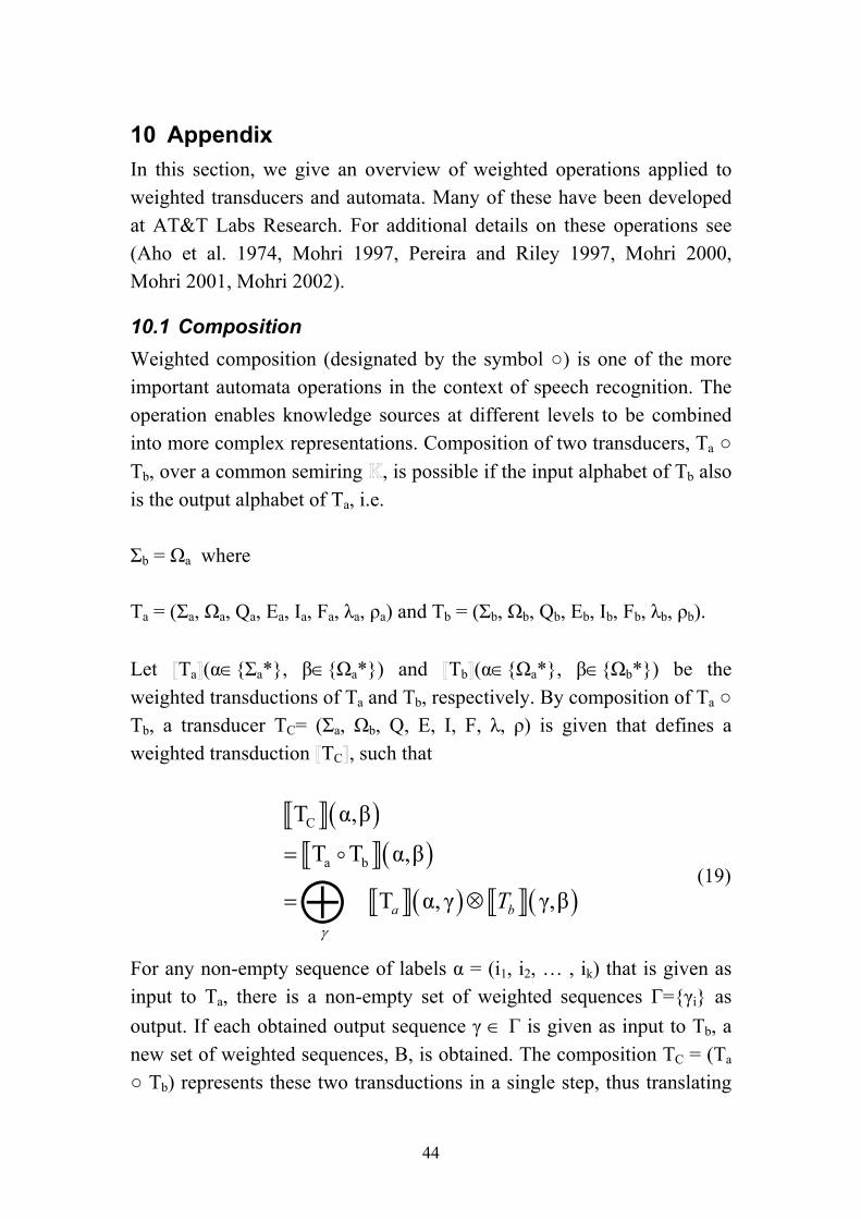
10 Appendix In this section, we give an overview of weighted operations applied to weighted transducers and automata. Many of these have been developed at AT&T Labs Research. For additional details on these operations see (Aho et al. 1974, Mohri 1997, Pereira and Riley 1997, Mohri 2000, Mohri 2001, Mohri 2002).

10.1 Composition Weighted composition (designated by the symbol ) is one of the more important automata operations in the context of speech recognition. The operation enables knowledge sources at different levels to be combined into more complex representations. Composition of two transducers, Ta Tb, over a common semiring , is possible if the input alphabet of Tb also is the output alphabet of Ta, i.e. Σb = Ωa where Ta = (Σa, Ωa, Qa, Ea, Ia, Fa, λa, ρa) and Tb = (Σb, Ωb, Qb, Eb, Ib, Fb, λb, ρb). Let Ta (α∈Σa*, β∈Ωa*) and Tb (α∈Ωa*, β∈Ωb*) be the weighted transductions of Ta and Tb, respectively. By composition of Ta Tb, a transducer TC= (Σa, Ωb, Q, E, I, F, λ, ρ) is given that defines a weighted transduction TC , such that

( )( )

( ) ( )

C

a b

T α,β

T T α,β

T α, γ γ,βa bTγ

=

= ⊗⊕ (19)

For any non-empty sequence of labels α = (i1, i2, … , ik) that is given as input to Ta, there is a non-empty set of weighted sequences Γ=γi as output. If each obtained output sequence γ ∈ Γ is given as input to Tb, a new set of weighted sequences, B, is obtained. The composition TC = (Ta Tb) represents these two transductions in a single step, thus translating

44

any sequence in α to a set of sequences B. The weight of each obtained sequence is the ⊗-product of the weights.

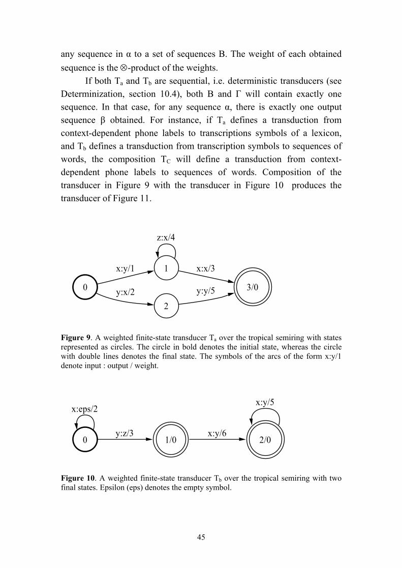
If both Ta and Tb are sequential, i.e. deterministic transducers (see Determinization, section 10.4), both B and Γ will contain exactly one sequence. In that case, for any sequence α, there is exactly one output sequence β obtained. For instance, if Ta defines a transduction from context-dependent phone labels to transcriptions symbols of a lexicon, and Tb defines a transduction from transcription symbols to sequences of words, the composition TC will define a transduction from context-dependent phone labels to sequences of words. Composition of the transducer in Figure 9 with the transducer in Figure 10 produces the transducer of Figure 11.

0

1x:y/1

2y:x/2

z:x/4

3/0

x:x/3

y:y/5

Figure 9. A weighted finite-state transducer Ta over the tropical semiring with states represented as circles. The circle in bold denotes the initial state, whereas the circle with double lines denotes the final state. The symbols of the arcs of the form x:y/1 denote input : output / weight.

0

x:eps/2

1/0y:z/3

2/0x:y/6

x:y/5

Figure 10. A weighted finite-state transducer Tb over the tropical semiring with two final states. Epsilon (eps) denotes the empty symbol.

45

0

1x:z/4

4

y:eps/4

2z:y/10

3/0x:y/9

5/0y:z/8

z:y/9

x:y/8

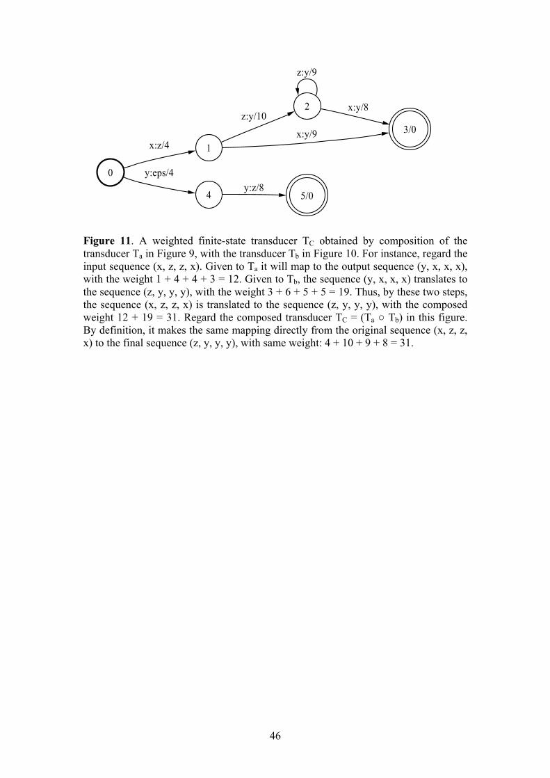
Figure 11. A weighted finite-state transducer TC obtained by composition of the transducer Ta in Figure 9, with the transducer Tb in Figure 10. For instance, regard the input sequence (x, z, z, x). Given to Ta it will map to the output sequence (y, x, x, x), with the weight 1 + 4 + 4 + 3 = 12. Given to Tb, the sequence (y, x, x, x) translates to the sequence (z, y, y, y), with the weight 3 + 6 + 5 + 5 = 19. Thus, by these two steps, the sequence (x, z, z, x) is translated to the sequence (z, y, y, y), with the composed weight 12 + 19 = 31. Regard the composed transducer TC = (Ta Tb) in this figure. By definition, it makes the same mapping directly from the original sequence (x, z, z, x) to the final sequence (z, y, y, y), with same weight: 4 + 10 + 9 + 8 = 31.

46

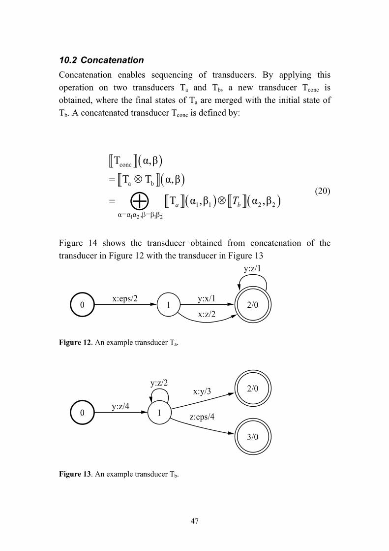
10.2 Concatenation Concatenation enables sequencing of transducers. By applying this operation on two transducers Ta and Tb, a new transducer Tconc is obtained, where the final states of Ta are merged with the initial state of Tb. A concatenated transducer Tconc is defined by:

( )( )

( ) ( )1 2 1 2

conc

a b

1 1 2 2,α=α α β=β β

T α,β

T T α,β

T α ,β α ,βa bT

= ⊗

= ⊗⊕ (20)

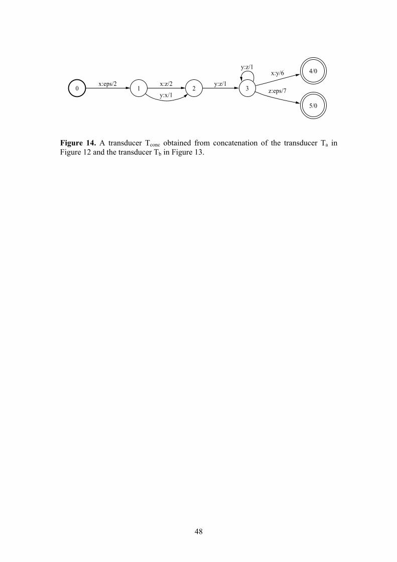
Figure 14 shows the transducer obtained from concatenation of the transducer in Figure 12 with the transducer in Figure 13

0 1x:eps/2

2/0y:x/1

x:z/2

y:z/1

Figure 12. An example transducer Ta.

0 1y:z/4

y:z/2 2/0x:y/3

3/0

z:eps/4

Figure 13. An example transducer Tb.

47

0 1x:eps/2

2x:z/2

y:x/13

y:z/1

y:z/1 4/0x:y/6

5/0

z:eps/7

Figure 14. A transducer Tconc obtained from concatenation of the transducer Ta in Figure 12 and the transducer Tb in Figure 13.

48

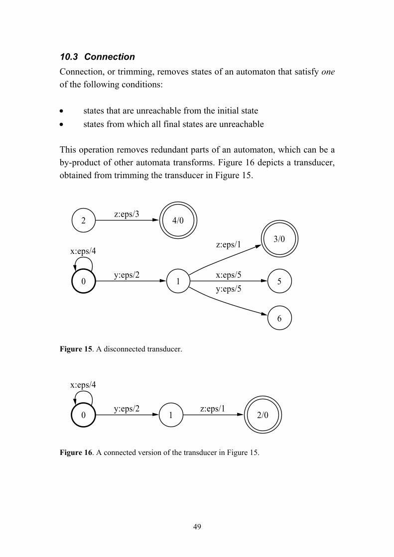
10.3 Connection Connection, or trimming, removes states of an automaton that satisfy one of the following conditions: • states that are unreachable from the initial state • states from which all final states are unreachable This operation removes redundant parts of an automaton, which can be a by-product of other automata transforms. Figure 16 depicts a transducer, obtained from trimming the transducer in Figure 15.

0

x:eps/4

1y:eps/2

3/0z:eps/1

5x:eps/5

6

y:eps/5

2 4/0z:eps/3

Figure 15. A disconnected transducer.

0

x:eps/4

1y:eps/2

2/0z:eps/1

Figure 16. A connected version of the transducer in Figure 15.

49

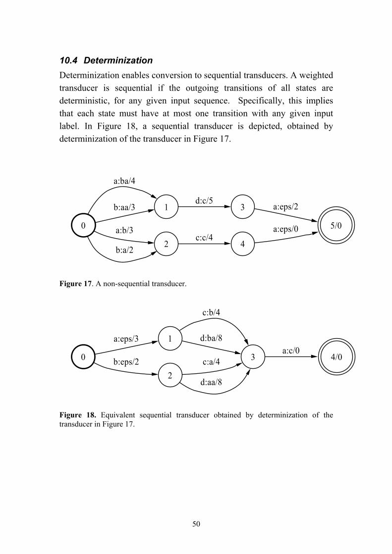
10.4 Determinization Determinization enables conversion to sequential transducers. A weighted transducer is sequential if the outgoing transitions of all states are deterministic, for any given input sequence. Specifically, this implies that each state must have at most one transition with any given input label. In Figure 18, a sequential transducer is depicted, obtained by determinization of the transducer in Figure 17.

Figure 17. A non-sequential transducer.

0

1

a:ba/4

b:aa/3

2a:b/3

b:a/2

3d:c/5

4c:c/4

5/0

a:eps/2

a:eps/0

0

1a:eps/3

2b:eps/2 3

c:b/4

d:ba/8

c:a/4

d:aa/8

4/0a:c/0

Figure 18. Equivalent sequential transducer obtained by determinization of the transducer in Figure 17.

50

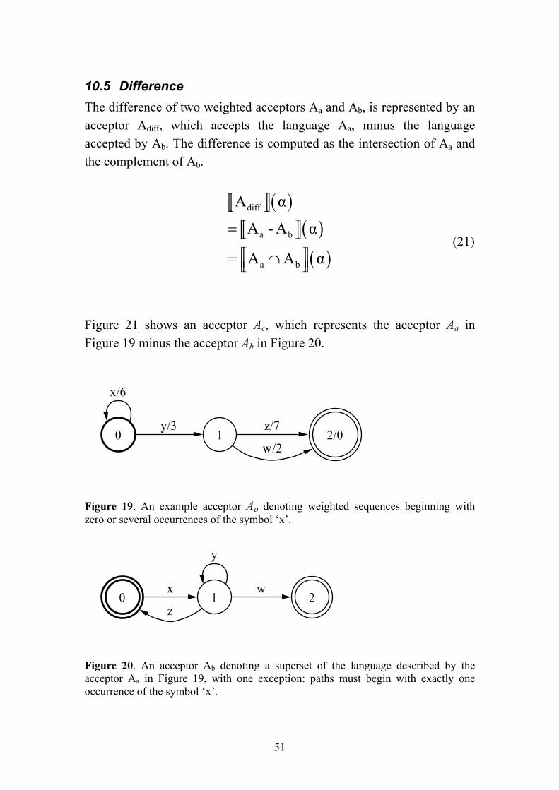
10.5 Difference The difference of two weighted acceptors Aa and Ab, is represented by an acceptor Adiff, which accepts the language Aa, minus the language accepted by Ab. The difference is computed as the intersection of Aa and the complement of Ab.

( )( )( )

diff

a b

a b

A α

A - A α

A A α

=

= ∩ (21)

Figure 21 shows an acceptor Ac, which represents the acceptor Aa in Figure 19 minus the acceptor Ab in Figure 20.

0

x/6

1y/3

2/0z/7

w/2

Figure 19. An example acceptor Aa denoting weighted sequences beginning with zero or several occurrences of the symbol ‘x’.

0 1x

z

y

2w

Figure 20. An acceptor Ab denoting a superset of the language described by the acceptor Aa in Figure 19, with one exception: paths must begin with exactly one occurrence of the symbol ‘x’.

51

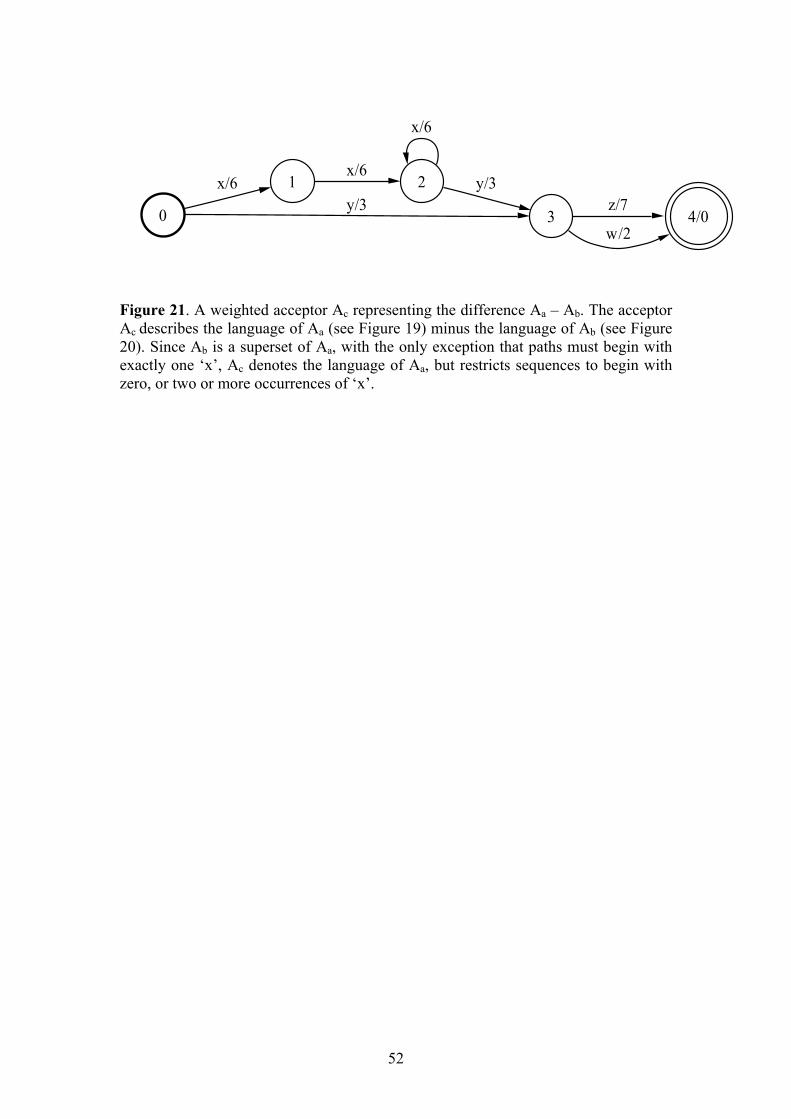
0

1x/6

3y/3

2x/6

4/0z/7

w/2

y/3

x/6

Figure 21. A weighted acceptor Ac representing the difference Aa – Ab. The acceptor Ac describes the language of Aa (see Figure 19) minus the language of Ab (see Figure 20). Since Ab is a superset of Aa, with the only exception that paths must begin with exactly one ‘x’, Ac denotes the language of Aa, but restricts sequences to begin with zero, or two or more occurrences of ‘x’.

52

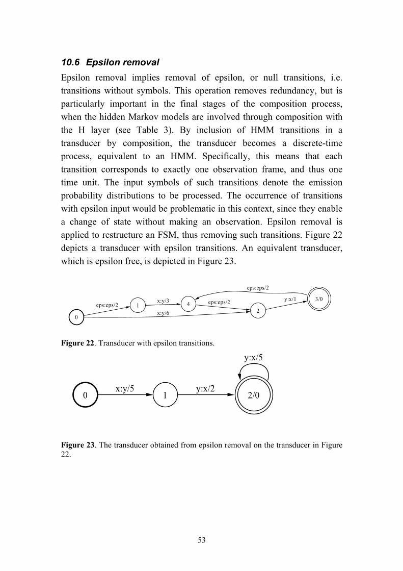
10.6 Epsilon removal Epsilon removal implies removal of epsilon, or null transitions, i.e. transitions without symbols. This operation removes redundancy, but is particularly important in the final stages of the composition process, when the hidden Markov models are involved through composition with the H layer (see Table 3). By inclusion of HMM transitions in a transducer by composition, the transducer becomes a discrete-time process, equivalent to an HMM. Specifically, this means that each transition corresponds to exactly one observation frame, and thus one time unit. The input symbols of such transitions denote the emission probability distributions to be processed. The occurrence of transitions with epsilon input would be problematic in this context, since they enable a change of state without making an observation. Epsilon removal is applied to restructure an FSM, thus removing such transitions. Figure 22 depicts a transducer with epsilon transitions. An equivalent transducer, which is epsilon free, is depicted in Figure 23.

0

1eps:eps/22x:y/6

4x:y/3 3/0y:x/1eps:eps/2

eps:eps/2

Figure 22. Transducer with epsilon transitions.

0 1x:y/5

2/0y:x/2

y:x/5

Figure 23. The transducer obtained from epsilon removal on the transducer in Figure 22.

53

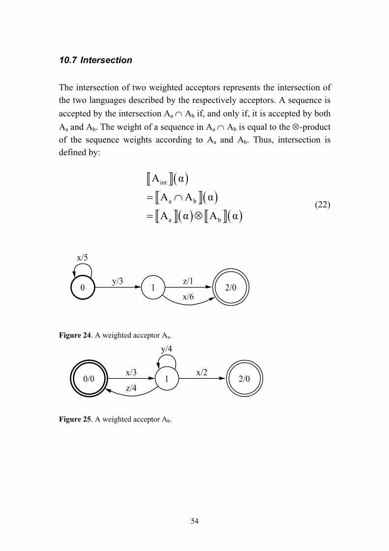
10.7 Intersection The intersection of two weighted acceptors represents the intersection of the two languages described by the respectively acceptors. A sequence is accepted by the intersection Aa ∩ Ab if, and only if, it is accepted by both Aa and Ab. The weight of a sequence in Aa ∩ Ab is equal to the ⊗-product of the sequence weights according to Aa and Ab. Thus, intersection is defined by:

( )( )

( ) ( )

int

a b

a b

A α

A A α

A α A α

= ∩

= ⊗ (22)

0

x/5

1y/3

2/0z/1

x/6

Figure 24. A weighted acceptor Aa.

0/0 1x/3

z/4

y/4

2/0x/2

Figure 25. A weighted acceptor Ab.

54

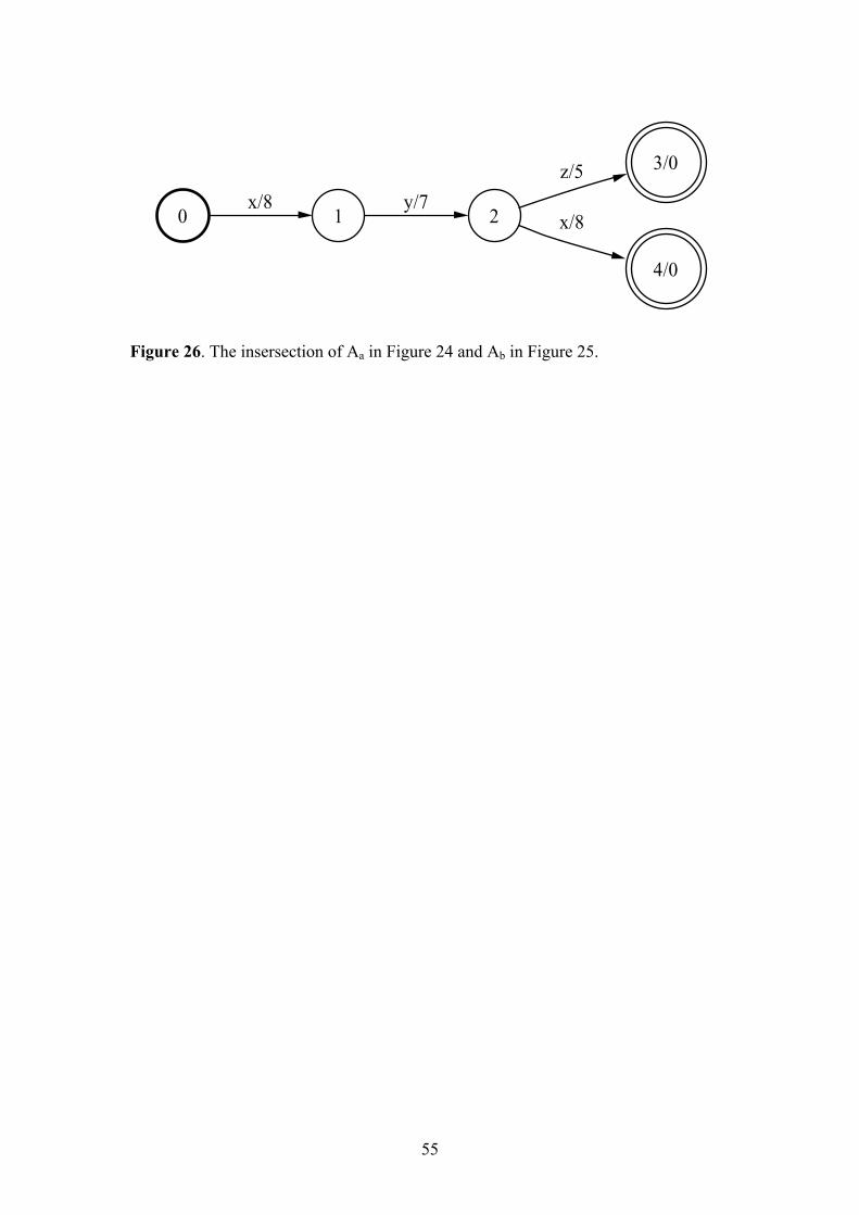
0 1x/8

2y/7

3/0z/5

4/0

x/8

Figure 26. The insersection of Aa in Figure 24 and Ab in Figure 25.

55

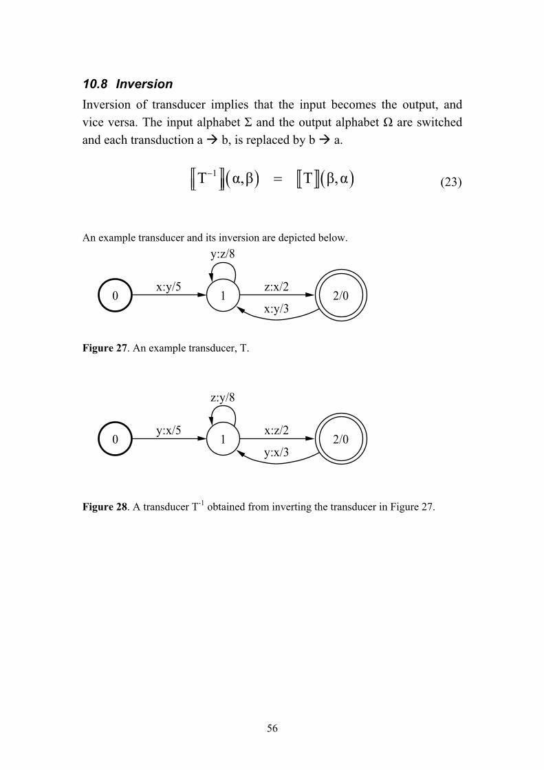
10.8 Inversion Inversion of transducer implies that the input becomes the output, and vice versa. The input alphabet Σ and the output alphabet Ω are switched and each transduction a b, is replaced by b a.

( ) ( )1T α,β T β,α− = (23)

An example transducer and its inversion are depicted below.

0 1x:y/5

y:z/8

2/0z:x/2

x:y/3

Figure 27. An example transducer, T.

0 1y:x/5

z:y/8

2/0x:z/2

y:x/3

Figure 28. A transducer T-1 obtained from inverting the transducer in Figure 27.

56

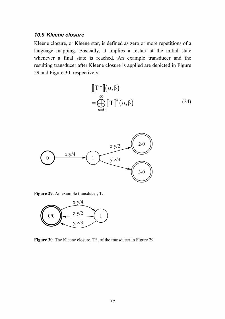
10.9 Kleene closure Kleene closure, or Kleene star, is defined as zero or more repetitions of a language mapping. Basically, it implies a restart at the initial state whenever a final state is reached. An example transducer and the resulting transducer after Kleene closure is applied are depicted in Figure 29 and Figure 30, respectively.

( )

(0

T * α,β

T α,βn

n=

∞=⊕ ) (24)

0 1x:y/4

2/0z:y/2

3/0

y:z/3

Figure 29. An example transducer, T.

0/0 1

x:y/4

z:y/2

y:z/3

Figure 30. The Kleene closure, T*, of the transducer in Figure 29.

57

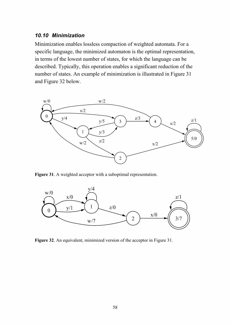
10.10 Minimization Minimization enables lossless compaction of weighted automata. For a specific language, the minimized automaton is the optimal representation, in terms of the lowest number of states, for which the language can be described. Typically, this operation enables a significant reduction of the number of states. An example of minimization is illustrated in Figure 31 and Figure 32 below.

0

w/0

1

y/43

x/2

y/3

2

z/2

y/5 4z/3

w/25/0

x/2

z/1

w/2

x/2

Figure 31. A weighted acceptor with a suboptimal representation.

0

w/0

1

x/0

y/1

y/4

2

z/0

w/7 3/7x/0

z/1

Figure 32. An equivalent, minimized version of the acceptor in Figure 31.

58

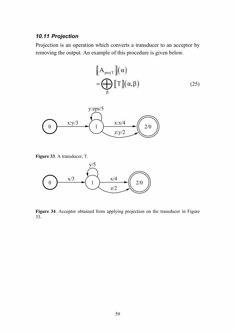
10.11 Projection Projection is an operation which converts a transducer to an acceptor by removing the output. An example of this procedure is given below.

( )

(proj T

β

A α

T α,β=⊕ ) (25)

0 1x:y/3

y:eps/5

2/0x:x/4

z:y/2

Figure 33. A transducer, T.

0 1x/3

y/5

2/0x/4

z/2

Figure 34. Acceptor obtained from applying projection on the transducer in Figure 33.

59

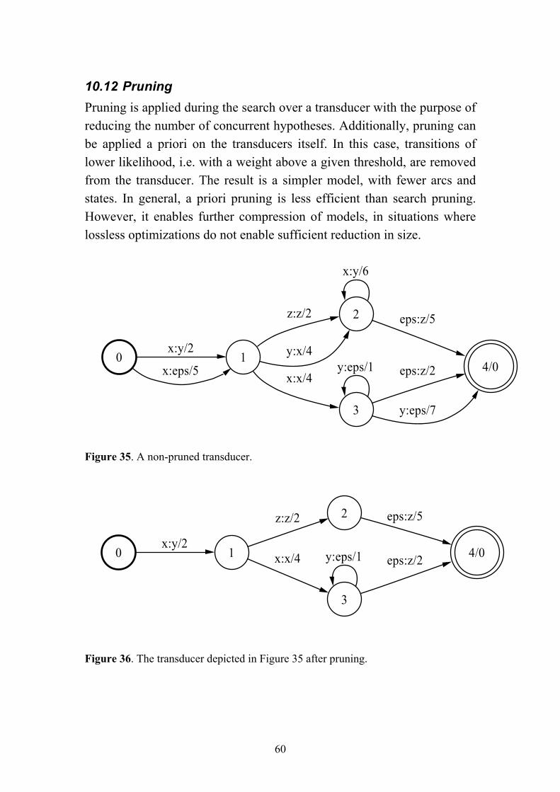
10.12 Pruning Pruning is applied during the search over a transducer with the purpose of reducing the number of concurrent hypotheses. Additionally, pruning can be applied a priori on the transducers itself. In this case, transitions of lower likelihood, i.e. with a weight above a given threshold, are removed from the transducer. The result is a simpler model, with fewer arcs and states. In general, a priori pruning is less efficient than search pruning. However, it enables further compression of models, in situations where lossless optimizations do not enable sufficient reduction in size.

0 1x:y/2

x:eps/5

2z:z/2

y:x/4

3

x:x/4

x:y/6

4/0

eps:z/5

y:eps/1 eps:z/2

y:eps/7

Figure 35. A non-pruned transducer.

0 1x:y/2

2z:z/2

3

x:x/4 4/0

eps:z/5

y:eps/1 eps:z/2

Figure 36. The transducer depicted in Figure 35 after pruning.

60

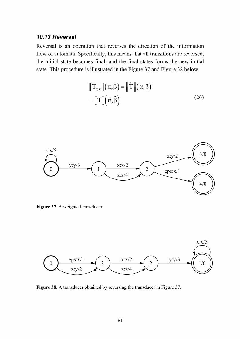
10.13 Reversal Reversal is an operation that reverses the direction of the information flow of automata. Specifically, this means that all transitions are reversed, the initial state becomes final, and the final states forms the new initial state. This procedure is illustrated in the Figure 37 and Figure 38 below.

( ) ( )

( )revT α,β T α,β

T α,β

=

= (26)

0

x:x/5

1y:y/3

2x:x/2

z:z/4

3/0z:y/2

4/0

eps:x/1

Figure 37. A weighted transducer.

0 3eps:x/1

z:y/22

x:x/2

z:z/41/0

x:x/5

y:y/3

Figure 38. A transducer obtained by reversing the transducer in Figure 37.

61

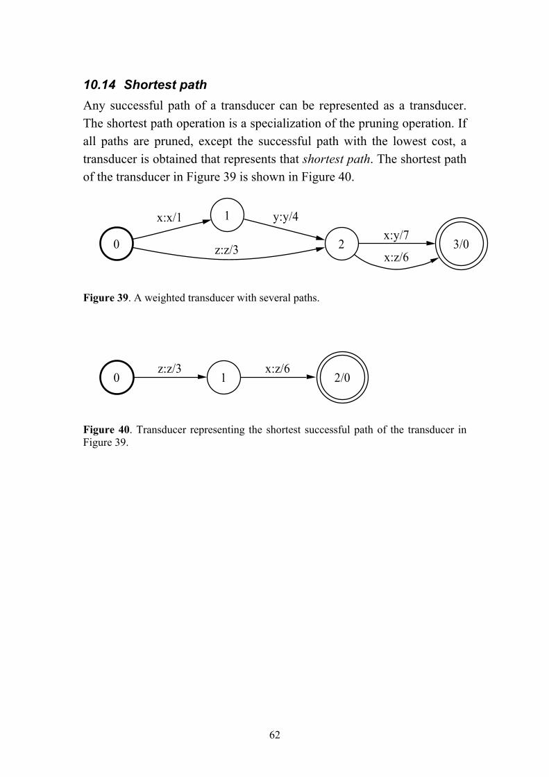
10.14 Shortest path Any successful path of a transducer can be represented as a transducer. The shortest path operation is a specialization of the pruning operation. If all paths are pruned, except the successful path with the lowest cost, a transducer is obtained that represents that shortest path. The shortest path of the transducer in Figure 39 is shown in Figure 40.

0

1x:x/1

2z:z/3

y:y/4

3/0x:y/7

x:z/6

Figure 39. A weighted transducer with several paths.

0 1z:z/3

2/0x:z/6

Figure 40. Transducer representing the shortest successful path of the transducer in Figure 39.

62

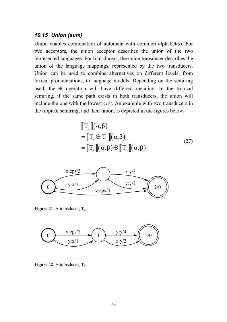
10.15 Union (sum) Union enables combination of automata with common alphabet(s). For two acceptors, the union acceptor describes the union of the two represented languages. For transducers, the union transducer describes the union of the language mappings, represented by the two transducers. Union can be used to combine alternatives on different levels, from lexical pronunciations, to language models. Depending on the semiring used, the ⊕ operation will have different meaning. In the tropical semiring, if the same path exists in both transducers, the union will include the one with the lowest cost. An example with two transducers in the tropical semiring, and their union, is depicted in the figures below.

( )( )

( ) ( )

u

a b

a b

T α,β

T T α,β

T α, β T α, β

= ⊕

= ⊕ (27)

0

1x:eps/3

y:x/2 2/0z:eps/4

x:y/3

y:y/2

Figure 41. A transducer, Ta.

0 1x:eps/2

y:x/12/0

y:y/4

z:y/2

Figure 42. A transducer, Tb.

63

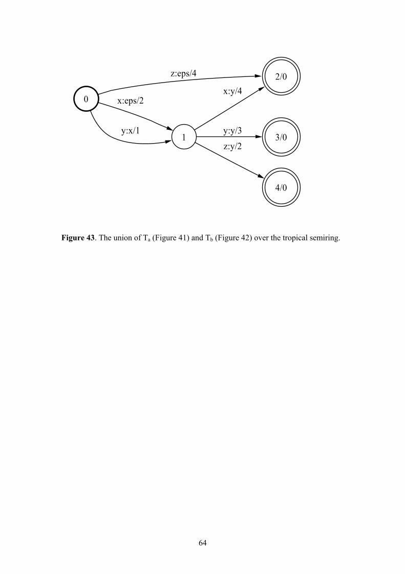
0

1

x:eps/2

y:x/1

2/0z:eps/4

x:y/4

3/0y:y/3

4/0

z:y/2

Figure 43. The union of Ta (Figure 41) and Tb (Figure 42) over the tropical semiring.

64

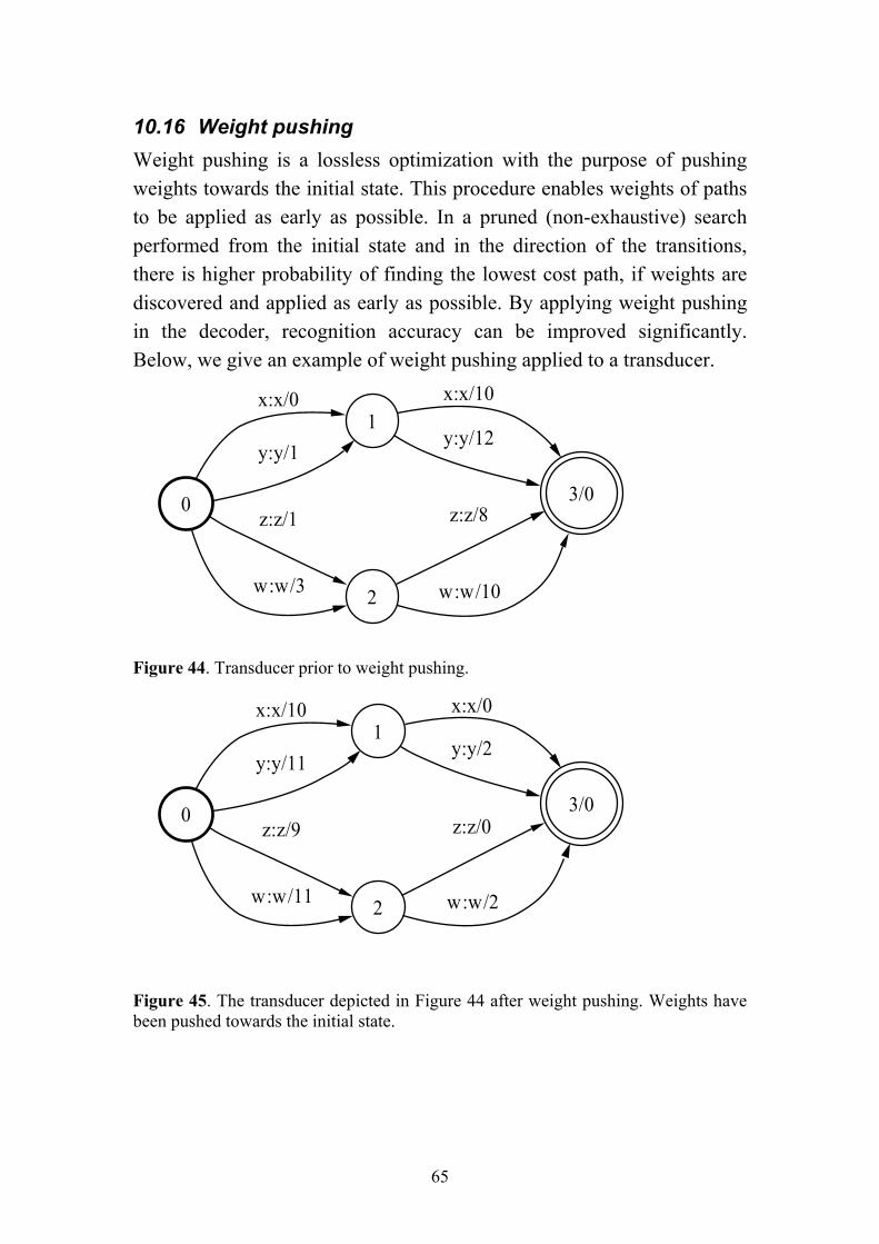
10.16 Weight pushing Weight pushing is a lossless optimization with the purpose of pushing weights towards the initial state. This procedure enables weights of paths to be applied as early as possible. In a pruned (non-exhaustive) search performed from the initial state and in the direction of the transitions, there is higher probability of finding the lowest cost path, if weights are discovered and applied as early as possible. By applying weight pushing in the decoder, recognition accuracy can be improved significantly. Below, we give an example of weight pushing applied to a transducer.

0

1x:x/0

y:y/1

2

z:z/1

w:w/3

3/0

x:x/10

y:y/12

z:z/8

w:w/10

Figure 44. Transducer prior to weight pushing.

0

1x:x/10

y:y/11

2

z:z/9

w:w/11

3/0

x:x/0

y:y/2

z:z/0

w:w/2

Figure 45. The transducer depicted in Figure 44 after weight pushing. Weights have been pushed towards the initial state.

65